Specific Emitter Identification Based on Transient Energy ...

Progress In Electromagnetics Research C, Vol. 44, 67–82, 2013

SPECIFIC EMITTER IDENTIFICATION BASED ONTRANSIENT ENERGY TRAJECTORY

Ying-Jun Yuan*, Zhi-Tao Huang, and Zhi-Chao Sha

College of Electronic Science and Engineering, National University ofDefense Technology, Changsha, Hunan 410073, P. R. China

Abstract—Specific emitter identification (SEI) is the technique whichidentifies the individual emitter based on the RF fingerprint of signal.Most existing SEI techniques based on the transient RF fingerprint aresensitive to noise and need different variables for transient detectionand RF fingerprint extraction. This paper proposes a novel SEItechnique for the common digital modulation signals, which is robustto Gaussian noise and can avoid the problem that different variablesare needed for transient detection and RF fingerprint extraction. Thismakes the technique more practical. The technique works based onthe signal’s energy trajectory acquired by the fourth order cumulants.A relative smoothness measure detector is used to detect the startingpoint and endpoint of the transient signal. The polynomial fittingcoefficients of the energy trajectory and transient duration form the RFfingerprint. The principal component analysis (PCA) technique is usedto reduce the feature vector’s dimension, and a support vector machine(SVM) classifier is used for classification. The signals captured fromeight mobile phones are used to test the performance of the technique,and the experimental results demonstrate that it has good performanceeven at low SNR levels.

1. INTRODUCTION

The SEI technique is very significant for the wireless spectrummanagement, security of Wi-Fi network and cognitive radio network,because the forgery of the RF fingerprint of a specific emitter is difficultas it is comparable to human fingerprint [1]. When an emitter isturned on, the signal goes through a transient state, the transient state

Received 7 August 2013, Accepted 16 September 2013, Scheduled 21 September 2013* Corresponding author: Ying-Jun Yuan ([email protected]).

68 Yuan, Huang, and Sha

is caused by a combination of effects and has unique and availablefeatures for SEI. SEI based on the transient signal requires two keystages: detection of the transients and extraction of the RF fingerprint.

The problem of detection of the transients has been studied as achange point detection problem. In [2], a method based on the variancefractal dimension is reported. This approach is based on the fact thatthe fractal dimension of the channel noise and the turn-on transientdiffer from each other. The change in the fractal dimension is thendetected by comparing the difference with a threshold. However, theselection of a threshold value is difficult because the noise is variable.In [3], a Bayesian step change detector based on fractal trajectory isreported which does not require a threshold. The method is suited forthe VHF radios where there is a step change in the power level at thestarting point of transients. However, the output power level of sometransients change slowly, e.g., Wi-Fi. For the problem, a Bayesianramp change detector is reported in [4]. Both approaches in [3, 4]are based on the fact that amplitude features of the channel noise andtransient are different, so they are sensitive to noise. Another approachis proposed in [5], based on the fact that the slope of the signal phasebecomes and remains linear from the starting point. This methodis insensitive to noise and interference, and the detection of startingpoint of transient signal has an error of about 150 points. In [6, 7],the method of independent component analysis (ICA) is proposed toextract the desired signal from the noise, and it is effective but requireshigh computation resources.

In some previous researches, the endpoint of transient signal hasnot been detected. In [8, 9], the end of the transient has been identifiedin an experimental manner. But in order to estimate the transientduration which can be used as a part of RF fingerprint [10, 11],detection of endpoint is necessary. In [11], the cusum algorithm basedon discrete variance has been used to detect the starting point andendpoint. However, an absolute threshold value difficult to confirm isneeded.

The RF fingerprint of transient signal has been mainly extractedfrom the amplitude, frequency, phase and the energy envelope inprevious researches. Hall et al. have utilized frequency and amplitudeinformation to create the RF fingerprint for identifying WLAN andBluetooth transmitters [8, 9]. Afolabi et al. have used a simulationmodel and formed the RF fingerprints by extracting six features fromthe preprocessed transient signal using amplitude, phase and frequencyprofile [12]. VHF radios have been identified by Ellis and Serinken withRF fingerprints created from amplitude and phase information [13].Xu et al. have used empirical mode decompositions to acquire the

Progress In Electromagnetics Research C, Vol. 44, 2013 69

amplitude and time-frequency distribution as RF fingerprint [14]. UrRehman et al. have formed the RF fingerprint by extracting six featuresfrom the energy envelope [10]. Zhao et al. have used the polynomialfitting coefficients of the energy envelope as the RF fingerprint [15].Based on wavelet theory, transient signal is decomposed and thecoefficients of wavelet have been formed as the RF fingerprint [9, 16].

Mostly, the previous researches are carried out in a laboratoryenvironment. The SNR of signal is usually high, but in a practicalapplication environment, the SNR of the captured signals wouldbe lower, so the susceptibility of the technique to noise should beconsidered. In many previous researches, the detection of transient andextraction of fingerprint need to calculate different variables, which isnot conducive to the practical application.

In this paper, a novel and more practical technique of SEI isproposed. The technique includes a complete classification system:signal acquisition, transient detection, RF fingerprint extraction andclassifier. The performance of the technique is tested by the signalsfrom eight mobile phones.

The rest of the paper is organized as follows. In Section 2, thesignal acquisition system of mobile phones is illustrated. In Section 3,how the energy trajectory is acquired is explained. In Sections 4and 5, the extraction process of transient signal and RF fingerprintare explained. Experimental results and conclusion are discussed inSections 6 and 7, respectively.

2. SIGNAL ACQUISITION

A signal acquisition system, shown in Fig. 1, is designed to collectsignals from mobile phones. A digital receiver (20 MHz ∼ 4000MHz)connected to a Yagi antenna converts the radio frequency signalsto intermediate frequency (IF) 70 MHz and a Leroy 8500 A digitaloscilloscope is used to collect the IF signal. The signals are sampledat a rate of 500 Msps, and the bandwidth of the receiver is 20 MHz.Then the captured signals are transferred to a computer via local areanetwork (LAN) and stored in digital format for further processing. Thetransient signals are collected from four Nokia 5230, two MotorolaMe525 and two Xiaomi mobile phones. The mobile phones work inGlobal System for Mobile communication (GSM) networks. The radiofrequency is 890–909 MHz. The modulation type is minimum shiftkeying (MSK), and the multiple access is time division multiple address(TDMA). Matlab2009b is used to analyze the transient signals.


Oscilloscope

Mobile phone

Digital receiver

IF=70MHz

GSM signal

890-909MHz

Data

processing

LAN

Yagi Antenna

Figure 1. Signal acquisition system.

3. EXTRACTION OF ENERGY TRAJECTORY

3.1. The Basic Knowledge of Higher Order Cumulants

Higher order cumulants (HOC) can describe the higher order statisticalcharacteristic of random process. There is an important feature thatthe higher order cumulants (greater than second order) of Gaussiannoise are permanent zero. So HOC can suppress Gaussian noise. Thethird order cumulants are permanent zero when the probability densityfunction of signal is symmetrical, so the fourth order cumulants areproposed to detect the transient signal and extract the RF fingerprintin this paper. For a zero-mean complex stochastic process X(t), itsp-order hybrid moment can be expressed as follows [17]:

Mpq = E[X (t)p−q X∗ (t)q] , (1)

where * denotes the conjugate function, and the fourth order cumulantsof X(t) are calculated as follows [17]:

C40 = Cum (X, X, X,X) = M40 − 3 (M20)2 , (2)

C41 = Cum (X, X, X,X∗) = M41 − 3M20M21, (3)

C42 = Cum (X, X, X∗, X∗) = M42 − |M20|2 − 2 (M21)2 (4)

Suppose that the signal serial is independent identicallydistributed, and that E is the signal energy, the fourth order cumulants’theoretical values of the common digital modulation signals are shownin Table 1 [17–19].


Table 1. Theoretical values of the common digital modulation signals’fourth order cumulants.

Modulationtype

|C40| |C41| |C42|2ASK 2E2 2E2 2E2

4ASK 1.36E2 1.36E2 1.36E2

BPSK 2E2 2E2 E2

QPSK E2 0 E2

OQPSK E2 0 E2

π/4−QPSK 0 0 E2

(M)PSK(M > 4) 0 0 E2

2/4/8FSK 0 0 E2

MSK 0 0 E2

GMSK 0 0 E2

(M)QAMkE 2 (k

depends on M)0

kE 2 (kdepends on M)

3.2. Signal Model

Typical transmission data, such as those shown in Fig. 2, containGaussian channel noise followed by the transient signal and the stablesignal. So the transmission data can be modeled as follows:

di =

{n (i) if 1 ≤ i < mst (i) + n (i) if m ≤ i ≤ kss (i) + n (i) if k + 1 ≤ i ≤ N

, (5)

where di is the data sample at time instant i, N the number of samples,m the starting point of the transient signal, k the endpoint, n(i) theGaussian channel noise, st(i) the transient signal, and ss(i) the stablesignal.

As can be seen from Table 1, the absolute value of C42 iskE 2 for the common digital modulation signals, and k depends onthe modulation type. So in this paper, the square root of C42 isused to acquire the energy trajectory which can express the energydistribution of signal. To acquire the energy trajectory of signal, asliding rectangular window is used to calculate the local C42. Thelength of the window is Lwnd, and the sliding length is Lslide. When


0 1000 2000 3000 4000 5000 6000 7000-1

-0.5

0

0.5

1

1.5

Samples

Am

pli

tude(

norm

aliz

ed)

Noise

Transient signal Stable signal

Figure 2. Typical transmissiondata from a Nokia 5230 mobilephone.

0 100 200 300 400 500 6000

0.5

1

1.5

Number of Slide

Ener

gy T

raje

ctory

(norm

aliz

ed)

tHoc

sHoc

nHoc

Figure 3. The energy trajectoryof the signal shown in Fig. 2.

there are signal and noise in the window, the value of C42 only dependson the signal because the nature of HOC expressed as follows:

Cum [r (t)] = Cum [s (t)] + Cum [n (t)] = Cum [s (t)] , (6)

where r(t) = s(t) + n(t), s(t) is signal, n(t) the Gaussian noise, ands(t) and n(t) are independently distributed.

The energy trajectory can be modeled as follows:

Hoc (i) =

{Hocn (i) if 1 ≤ i < mHoct (i) if m ≤ i ≤ kHocs (i) if k + 1 ≤ i ≤ N

, (7)

where i denotes the i-th slide, Hoc(i) the corresponding√|C42|, N

the total of slide, m the first time that there is the transient signal inthe sliding window, k the last time that there is the transient signalin the sliding window, Hocn the

√|C42| of noise, Hoct the

√|C42| of

transient signal, and Hocs the√|C42| of stable signal. The normalized

energy trajectory of the signal shown in Fig. 2 is shown in Fig. 3. Thelength of the window Lwnd is 256, and the sliding length Lslide is 10.In order to represent the subtle feature of energy distribution, Lwnd

and Lslide cannot be too large, however Lwnd cannot be too small tosuppress the Gaussian noise effectively. In this paper, we find thatLwnd is 200 ∼ 300 and Lslide is 10 ∼ 30 seem to be suitable.

4. TRANSIENT SIGNAL EXTRACTION

Before extracting the transient features, we need to find the exact timewhen the transient starts and ends. It is significant because inaccuratedetection adversely affects the performance of feature extraction.


4.1. Transient Starting Point Detection

As can be seen from formula (7) and Fig. 3, the energy trajectoryhas obvious characteristics. When there is only noise in the slidingwindow, theoretically, the value of Hocn should be zero, and throughexperimental verification, it is usually approximate but not zerobecause the length of the sliding window is not enough. When there isthe transient signal in the sliding window, the energy trajectory beginsto rise, and when there is only stable signal, the Hocs value is stable.Theoretically, Hocs = kEs, and Es is the energy of the stable signal.

In this paper, we use a relative smoothness measure (RSM)detector which has an obvious characteristic at the starting pointand endpoint to detect the transients. The other sliding rectangularwindow is used to calculate the output of the RSM-detector as follows:

T (i) =i+LT−1∑

j=i

Hoc (j)2/

i+LT−1∑

j=i

Hoc (j)

2

1 ≤ i ≤ N − LT , (8)

where i denotes i-th slide, LT the length of the sliding window, N thelength of the energy trajectory, and T (i) the output of the detector.The window slides one point each time. It is obvious that 0 < T (i) ≤ 1.

As can be seen from formula (7) and Fig. 3, a hypothesis isreasonable that there is a point ps > m (m is the first point of Hoct),when 1 6 i 6 ps, l > ps, Hoc(l) À Hoc (i). Because the Hocn beforem is approximate zero and the energy of transient signal in the i-th(m 6 i 6 ps) sliding window is little. When n = ps +2−LT , the RSM-detector output value can be approximately calculated as follows:

T (n) =

ps+1∑j=ps+2−LT

Hoc (j)2

(ps+1∑

j=ps+2−LT

Hoc (j)

)2

=

(ps∑

j=ps+2−LT

Hoc (j)2+Hoc (ps+1)2)

(ps∑

j=ps+2−LT

Hoc (j)+Hoc (ps+1)

)2 ≈Hoc (ps + 1)2

Hoc (ps + 1)2=1 (9)

It can be deduced from formula (9) that the RSM-detector willoutput a maximum near the starting point of the transient signal.Mostly, the transient signal should start before the maximum. In orderto find the more exact starting point, a Bayesian change detector in [3]


is used to detect the change point before the maximum. The detectoris given as follows:

p ({m}|T )α1√

m (N −m)

×

N∑

i=1

T (i)2− 1m

(m∑

i

T (i)

)2

− 1N−m

(N∑

i=m+1

T (i)

)2−(N−2

2 )

, (10)

where N is the corresponding point of the maximum, 1 6 m < N ,and T (i) is the i-th RSM-detector output. The energy trajectory ofthe transient signal shown in Fig. 3 with corresponding RSM-detectoroutput curve (LT = 50) is shown in Fig. 4. The Bayesian methodis used to test each point before N as a potential change point usingthe expression p({m}|T ). The corresponding probability density is alsoshown in Fig. 4.

0 50 100 150 200 250 3000

0.05

0.1

Number of Slide

En

erg

y

Tra

ject

ory

0 50 100 150 200 250 3000

0.5

1

Number of Slide

RS

M-d

etec

tor

Ou

tpu

t

0 50 100 150 200 250 3000

0.5

1

1.5

Number of Slide

Pro

bab

ilit

y D

ensi

ty

(no

rmal

ized

)

Maximum point 127

Change point 126

Figure 4. Energy trajectory, RSM-detector curve and change pointdetection result.

As can be seen from Fig. 4, when the transient signal starts,there is a maximum in the RSM-detector output curve, and theprobability density has a peak which is the change point Pc. Wecan deduce that the transient signal starts at the endpoint of Pc-thsliding window which is used to calculate the RSM-detector outputcurve. The endpoint of Pc-th sliding window is Pc + LT in the energytrajectory, which means that the sliding window which is used to getthe energy trajectory slides Pc + LT times. It is reasonable to deducethat the starting point of transient signal is the middle point between


the endpoint of Pc+LT−1-th and Pc+LT -th slide. The endpoint of thePc +LT −1-th slide in the samples is (Pc + LT − 2)×Lslide +Lwnd andthe Pc + LT -th slide is (Pc + LT − 1)× Lslide + Lwnd. So the startingpoint in the samples can be calculated as follows:

Pstart = (Pc + LT − 1.5)× Lslide + Lwnd, (11)

The detected result is 2001 in Fig. 4 and the actual observed value is2015, so the detection error is 14 samples.

4.2. Transient Endpoint Detection

When the signal is stable, theoretically, Hocs = kEs. The RSM-detector output value can be calculated as follows:

T (n) =n+LT−1∑

j=n

Hoc (j)2/

n+LT−1∑

j=n

Hoc (j)

2

= LT × (kEs)2/

(LT × kEs)2 = 1/LT , (12)

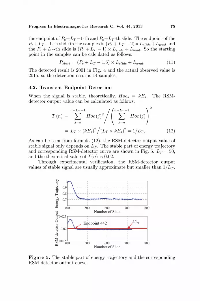
As can be seen from formula (12), the RSM-detector output value ofstable signal only depends on LT . The stable part of energy trajectoryand corresponding RSM-detector curve are shown in Fig. 5. LT = 50,and the theoretical value of T (n) is 0.02.

Through experimental verification, the RSM-detector outputvalues of stable signal are usually approximate but smaller than 1/LT .

400 500 600 700 800

0.7

0.8

0.9

1

Number of Slide

Ener

gy T

raje

ctory

400 500 600 700 8000.015

0.02

0.025

Number of Slide

RS

M-d

etec

tor

Outp

ut

Endpoint 442 1/L T

Figure 5. The stable part of energy trajectory and the correspondingRSM-detector output curve.


So the endpoint of transients PE can be defined as the point that after itnearly all values are smaller than 1/LT , which means that all values inthe energy trajectory after PE-th slide are stable. In the PE-th slidingwindow, there may be both transient signal and stable signal, so wesuppose that the endpoint is the middle point between the startingpoint and endpoint of PE-th slide. The starting point of PE-th slide is(PE − 1)×Lslide + 1, and the endpoint is (PE − 1)×Lslide + Lwnd, sothe corresponding endpoint in the samples can be calculated as follows:

PEnd = (PE − 1)× Lslide + 0.5× Lwnd, (13)

The detected result is 4538 in Fig. 4. The actual observed value is4598, and the detection error is 60 samples.

The duration of transient signal Td can be calculated as follows:

Td = (PEnd − Pstart)/Fs, (14)

where Fs is the sampling rate and PEnd−Pstart the number of samplesbetween the starting point and endpoint of the transient signal.

5. RF FINGERPRINT EXTRACTION ANDCLASSIFICATION

5.1. Fingerprint Extraction

As can be seen from Fig. 2 and Fig. 3, the energy trajectory caneffectively reflect the characteristics of the transient signal’s energydistribution. Eight normalized energy trajectories of the transientsignals from different mobile phones are shown in Fig. 6. From thestarting point, there are 5,000 samples for each signal and Lwnd = 256,Lslide = 20.

As can be seen from Fig. 6, the features of the energy trajectoriescan be used to form the effective RF fingerprint. The method of least-squares polynomial fitting is used to extract the features from theenergy trajectory, and the equation of least-squares polynomial fittingcan be expressed as follows:

y (x) = a0 + a1x + a2x2 + . . . + anxn, (15)

where a0, a1, a2, . . . , an are the coefficients to be determined, and n isthe order of the polynomial function. The fitting function must satisfythe minimum mean-square error (MSE), which can be expressed asfollows:

MSE =N∑

i=1

[y (xi)−Hoc (i)]2 (16)


0 50 100 150 2000

0.2

0.4

0.6

0.8

1

Number of Slide

Ener

gy T

raje

ctory

(norm

aliz

ed)

Nokia 5230 1

Nokia 5230 2

Nokia 5230 3

Nokia 5230 4

Xiaomi 1

Xiaomi 2

Moto Me525 1

Moto Me525 2

Figure 6. Normalized energytrajectories of transients fromeight mobile phones.

10 15 20 25 30 35 40 45 500

0.005

0.01

0.015

0.02

0.025

Order of The Polynomial

Mea

n M

SE

Figure 7. The mean MSE valuesin different order.

The least-squares algorithm based on QR decomposition (LSQR)presented in [20], which has a more stable behavior and can get a moreaccurate solution, is used to solve the least-squares problem and getthe coefficients.

The order n is important for the performance of the curve fit.In order to find a suitable order n, a set of 160 transient signals arechosen from 8 emitters to test, 20 transient signals from each one. Inthe experiment, the order n is 6 ∼ 50, and the mean MSE values ofcurve fit in each n are plotted in Fig. 7.

As can be seen from Fig. 7, when the order is 10 ∼ 40, the MSEis smaller, and that means the performance is better. When the orderis higher than 40, the MSE increases because of the waviness and end-effects [21]. The lower the order is, the less the computation is, sothe order n = 10 in this paper. However, the order depends on theactual situation. When the shape of the energy trajectory is complexor unknown, we suggest the higher order n may be suitable.

When n = 10, the 11 polynomial coefficients a0, a1, a2, . . . , a10

are acquired as the feature of energy trajectory. As can be seenfrom Fig. 6, the duration of transient signal Td acquired in Section 4is also an effective feature, so the RF fingerprint feature vectoris [Td, a0, a1, a2, . . . , a10].

5.2. Reduction of the Feature Vector’s Dimension

To reduce the dimension of the feature vector, principal componentanalysis (PCA) is used in this paper. PCA is a well-known statisticalmethod that has been used in various disciplines for data compression,redundancy and dimension reduction and feature extraction. It can


transform a set of correlated variables into a set of uncorrelatedvariables, which are ordered by decreasing variability and have a low-dimensional feature vector with low complexity. The low-dimensionalfeature vector can make the classifier work more effective. The effectof PCA for SEI has been verified [22], and the detailed informationabout PCA can be found in [22].

5.3. Classification

Support Vector Machine (SVM) is a machine intelligence algorithmbased on statistical learning theory, which is popular for patternrecognition. Its core idea is using a pre-selected non-linear mapping tomap an linear inseparable space to a linear separable high-dimensionalspace. In this space, a separating hyperplane with the largest margincan be found using the structural risk minimization principle, andthe method of finding the separating hyperplane can maximize thegeneralization ability of learning machine. The separating hyperplanecan maximize the space between different classes [23]. When the dataare separable, the classification function is defined as follows:

f (x) = sign (w · φ (x) + b) , (17)

where φ (x) is kernel function, and w and b determine the hyperplaneof the space. When the data are inseparable, the classification functionis defined as:

f (x) = sign

[(L∑

i=1

αiyiK (xi, xj)

)+ b

], (18)

where K (xi, xj) is kernel function, αi is i-th mode embeddeddimension, yi is i-th label. Detailed information about SVM can befound in [23–25].

6. EXPERIMENTAL RESULTS

In order to evaluate the performance of this technique, a set of 1200signals is created by capturing 150 signals from each one of the eightmobile phones. For each emitter, 50 of 150 transients are chosenrandomly to create a training set. The remaining 100 transientsare used as a test set. Each captured signal includes channel noise,transient and stable signal, and the length is 10000 samples. Firstly,the starting point and endpoint are estimated utilizing the methodin Section 4, then the transient energy trajectory is extracted andthe feature vector is acquired by polynomial fitting. The method ofPCA is used to reduce the dimension of the feature space. A SVM


classifier is created using the feature vectors of the training set, andits performance is evaluated by the feature vectors of the test set.

The signals are captured in a laboratory environment, so the SNRsof the captured signals are high. The detection accuracy of startingpoint and endpoint is tested using 800 high SNR transient signals. Thedetection error mean, which is the mean of the difference between thevisually observed value and the estimated value, is 16 samples for thestarting point and 50 samples for the endpoint. When the high SNRtraining and test signals arere applied to the classifier, the identificationrate is 99.5%.

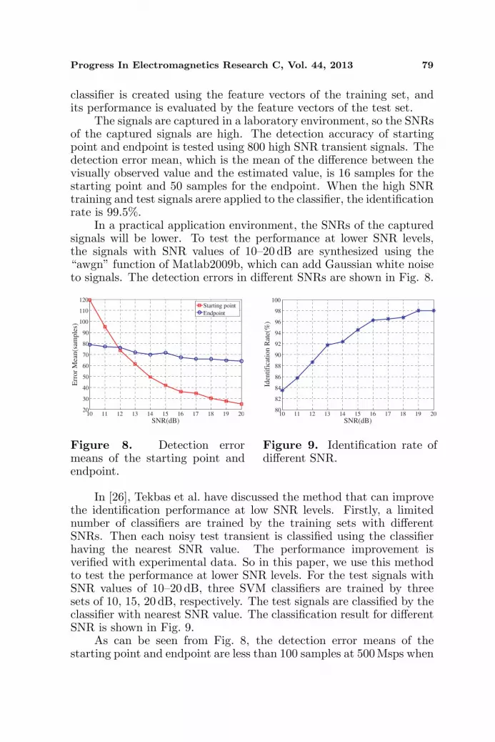
In a practical application environment, the SNRs of the capturedsignals will be lower. To test the performance at lower SNR levels,the signals with SNR values of 10–20 dB are synthesized using the“awgn” function of Matlab2009b, which can add Gaussian white noiseto signals. The detection errors in different SNRs are shown in Fig. 8.

10 11 12 13 14 15 16 17 18 19 2020

30

40

50

60

70

80

90

100

110

120

SNR(dB)

Err

or

Mea

n(s

amp

les)

Starting point

Endpoint

Figure 8. Detection errormeans of the starting point andendpoint.

10 11 12 13 14 15 16 17 18 19 2080

82

84

86

88

90

92

94

96

98

100

SNR(dB)

Identi

ficati

on R

ate

(%)

Figure 9. Identification rate ofdifferent SNR.

In [26], Tekbas et al. have discussed the method that can improvethe identification performance at low SNR levels. Firstly, a limitednumber of classifiers are trained by the training sets with differentSNRs. Then each noisy test transient is classified using the classifierhaving the nearest SNR value. The performance improvement isverified with experimental data. So in this paper, we use this methodto test the performance at lower SNR levels. For the test signals withSNR values of 10–20 dB, three SVM classifiers are trained by threesets of 10, 15, 20 dB, respectively. The test signals are classified by theclassifier with nearest SNR value. The classification result for differentSNR is shown in Fig. 9.

As can be seen from Fig. 8, the detection error means of thestarting point and endpoint are less than 100 samples at 500Msps when


SNR > 10 dB. But the detection error mean increases fast when SNRreduces for the starting point detection and slowly for the endpointdetection because the energy at the starting point is so small that itcan be affected by noise more easily. As can be seen from Fig. 9, theidentification rate is more than 90% when SNR > 12 dB.

7. CONCLUSION

In this paper, a more practical SEI technique for the common digitalmodulation signals shown in Table 1 is proposed. The techniquedetects the transients and extracts the RF fingerprint based on theenergy trajectory of signal, and then a SVM classifier is used to identifyeight mobile phones.

In this technique, a RSM-detector is used to detect both startingpoint and endpoint of transient signal, which does not need an absolutethreshold and has good performance. The energy trajectory of signalis used to detect the transients and extract the RF fingerprint. Theproblem that different variables are needed for transient detection andRF fingerprint extraction is avoided. The energy trajectory is acquiredby fourth order cumulants which can suppress Gaussian noise, so thetechnique is robust to Gaussian noise. In order to test the performanceat low SNR levels, the signals with SNR values of 10–20 dB are usedto test. The experimental results demonstrate that the technique hasgood performance at low SNR.

REFERENCES

1. Danev, B., H. Luecken, S. Capkun, and K. EI Defrawy, “Attackson physical-layer identification,” Proc. ACM Conf. on WirelessNetwork Security, 89–98, 2010.

2. Shaw, D. and W. Kinsner, “Multifractal modeling of radiotransmitter transients for classification,” Proc. WESCANEX’97,306–312, 1997.

3. Ureten, O. and N. Serinken, “Detection of radio transmitter turn-on transients,” Electronics Letters, Vol. 35, No. 23, 1996–1997,1999.

4. Ureten, O. and N. Serinken, “Bayesian detection of Wi-Fitransmitter RF fingerprints,” Electronics Letters, Vol. 41, No. 6,373–374, 2005.

5. Hall, J., M. Barbeau, and E. Kranakis, “Detection of transientin radio frequency fingerprinting using signal phase,” Proceedings


of the 3rd IASTED Int. Conf. on Wireless and OpticalCommunications, 13–18, 2003.

6. Lee, T. W., Independent Component Analysis: Theory andApplications, Kluwer Academic Publishers, 1999.

7. Donelli, M., “A rescue radar system for the detection of victimstrapped under rubble based on the independent componentanalysis algorithm,” Progress In Electromagnetics Research M,Vol. 19, 173–181, 2011.

8. Hall, J., M. Barbeau, and E. Kranakis, “Enhancing intrusion de-tection in wireless networks using radio frequency fingerprinting,”Proceedings of the 3rd IASTED International Conference on Com-munications, Internet and Information Technology (CIIT), 201–206, 2004.

9. Hall, J., M. Barbeau, and E. Kranakis, “Detecting rogue devicesin bluetooth networks using radio frequency fingerprinting,”IASTED International Conference on Communications andComputer Networks, 108–113, 2006.

10. Ur Rehman, S., K. Sowerby, and C. Coghill, “RF fingerprintextraction from the energy envelope of an instantaneoustransient signal,” Australian Communications Theory Workshop(AusCTW), 90–95, 2012.

11. Bonne Rasmussen, K. and S. Capkun, “Implications of radiofingerprinting on the security of sensor networks,” Proceedings ofthe Third International Conference on Security and Privacy inCommunications Networks and the Workshops, IEEE, 331–340,2007.

12. Afolabi, O., K. Kim, and A. Ahmad, “On secure spectrumsensing in cognitive radio networks using emitters electromagneticsignature,” Proceedings of 18th Internatonal Conference onComputer Communications and Networks, 1–5, 2009.

13. Ellis, K. and N. Serinken, “Characteristics of radio transmitterfingerprints,” Radio Science, Vol. 36, No. 4, 585–597, 2001.

14. Xu, J., H. Zhao and T. Liang, “Method of empirical modedecompositions in radio frequency fingerprint,” 2010 InternationalConference on Microwave and Millimeter Wave Technology(ICMMT), 1275–1278, 2010.

15. Zhao, C., L. Huang, L. Hu, and Y. Yao, “Transient fingerprintfeature extraction for WLAN cards based on polynomial fitting,”The 6th International Conference on Computer Science &Education (ICCSE 2011), 1099–1102, 2011.

16. Klein, R. W., M. A. Temple, and M. J. Mendenhall, “Application


of wavelet-based RF fingerprinting to enhance wireless networksecurity,” Journal of Communications and Networks, 544–555,2009.

17. Wang, L. and Y. Ren, “Recognition of digital modulation signalsbased on high order cumulants and support vector machines,”ISECS International Colloquium on Computing, Communication,Control, and Management, 271–274, 2009.

18. Zhou, X., Y. Wu, and B. Yang, “Signal classification method basedon support vector machine and high-order cumulants,” WirelessSensor Network, 48–52, 2010.

19. Swami, A. and B. M. Sadler, “Hierarchical digital modulationclassification using cumulants,” IEEE Transactions on Communi-cations, Vol. 48, No. 3, 416–429, 2000.

20. Paige, C. and M. Saunders, “LSQR: An algorithm for sparse linearequations and sparse least squares,” ACM Trans. Math. Software,Vol. 8, 43, 1982.

21. Robert-Granie, C., J.-L. Foulley, E. Maza, and R. Rupp,“Statistical analysis of somatic cell scores via mixed modelmethodology for longitudinal data,” Anim. Res, Vol. 53, 259–273,2004.

22. Xu, S., B. Huang, L. Xu, and Z. Xu, “Radio transmitterclassification using a new method of stray features analysiscombined with PCA,” Military Communications Conference(MILCOM 2007), 1–5, 2007.

23. Burges, C. J. C., “A tutorial on support vector machines forpattern recognition,” Data Mining and Knowledge Discovery, 121–167, 1998.

24. Bermani, E., A. Boni, A. Kerhet, and A. Massa, “Kernelsevaluation of SVM-based estimators for inverse scatteringproblems,” Progress In Electromagnetics Research, Vol. 53, 167–188, 2005.

25. Bermani, E., A. Boni, S. Caorsi, M. Donelli, and A. Massa, “Amulti-source strategy based on a learning-by-examples techniquefor buried object detection,” Progress In ElectromagneticsResearch, Vol. 48, 185–200, 2004.

26. Tekbas, O. H., O. Ureten, and N. Serinken, “Improvementof transmitter identification system for low SNR transients,”Electronics Letters, Vol. 40, No. 3, 192–183, 2004.

Specific Emitter Identification Based on Transient Energy ...

Documents

Transcript of Specific Emitter Identification Based on Transient Energy ...