Transient analysis of data-normalized adaptive filters
14
IEEE TRANSACTIONS ON SIGNAL PROCESSING, VOL. 51, NO. 3, MARCH 2003 639 Transient Analysis of Data-Normalized Adaptive Filters Tareq Y. Al-Naffouri and Ali H. Sayed, Fellow, IEEE Abstract—This paper develops an approach to the transient analysis of adaptive filters with data normalization. Among other results, the derivation characterizes the transient behavior of such filters in terms of a linear time-invariant state-space model. The stability of the model then translates into the mean-square stability of the adaptive filters. Likewise, the steady-state operation of the model provides information about the mean-square deviation and mean-square error performance of the filters. In addition to deriving earlier results in a unified manner, the approach leads to stability and performance results without restricting the regression data to being Gaussian or white. The framework is based on energy-conservation arguments and does not require an explicit recursion for the covariance matrix of the weight-error vector. Index Terms—Adaptive filter, data nonlinearity, energy-con- servation, feedback analysis, mean-square-error, stability, steady-state analysis, transient analysis. I. INTRODUCTION A DAPTIVE filters are, by design, time-variant and nonlinear systems that adapt to variations in signal statistics and that learn from their interactions with the environment. The success of their learning mechanism can be measured in terms of how fast they adapt to changes in the signal characteristics and how well they can learn given sufficient time (e.g., [1]–[3]). It is therefore typical to measure the performance of an adaptive filter in terms of both its transient performance and its steady-state performance. The former is concerned with the stability and convergence rate of an adaptive scheme, whereas the latter is concerned with the mean-square error that is left in steady state. There have been extensive works in the literature on the per- formance of adaptive filters with many ingenious results and approaches (e.g., [1]–[11]). However, it is generally observed that most works study individual algorithms separately. This is because different adaptive schemes have different nonlinear up- date equations, and the particularities of each case tend to re- quire different arguments and assumptions. In recent works [12]–[15], a unified energy-based approach to the steady-state and tracking performance of adaptive filters has been developed that makes it possible not only to treat algo- Manuscript received February 28, 2001; revised October 23, 2002. This work was supported in part by the National Science Foundation under Grants CCR -9732376, ECS-9820765, and CCR -0208573. The work of T. Y. Al-Naffouri was also partially supported by a fellowship from King Fahd University of Pe- troleum and Minerals, Saudi Arabia. The associate editor coordinating the re- view of this paper and approving it for publication was Dr. Xiang-Gen Xia. T. Y. Al-Naffouri is with the Electrical Engineering Department, Stanford University, Stanford, CA 94305 USA (e-mail: [email protected]). A. H. Sayed is with the Electrical Engineering Department, University of California, Los Angeles, CA 90095 USA (e-mail: [email protected]). Digital Object Identifier 10.1109/TSP.2002.808106 rithms uniformly but also to arrive at new performance results. This approach is based on studying the energy flow through each iteration of an adaptive filter, and it relies on an exact energy conservation relation that holds for a large class of adaptive fil- ters. This relation has been originally developed in [16]–[19] in the context of robustness analysis of adaptive filters within a de- terministic framework. It has since then been used in [12]–[15] as a convenient tool for studying the steady-state performance of adaptive filters within a stochastic framework as well. In this paper, we show how to extend the energy-based approach to the transient analysis (as opposed to the steady-state analysis) of adaptive filters. Such an extension is desirable since it would allow us, just as in the steady-state case, to bring forth sim- ilar benefits such as the convenience of a unified treatment, the derivation of stability and convergence results, and the weak- ening of some assumptions. In a companion article [20], we similarly extend the energy- conservation approach to study the transient behavior of adap- tive filters with error nonlinearities. A. Contributions of the Work The main contributions of the paper are as follows. a) In the next section, we introduce weighted estimation errors aswellasweightedenergynormsandrelatethesequantities through a fundamental energy relation. The main results of this section are summarized in Theorem 1. b) In Sections III and IV, we illustrate the mechanism of our approach for transient analysis by applying it to the LMS algorithm and its normalized version for Gaussian regres- sors. c) In Section V, we study the general case of adaptive algo- rithms with data nonlinearities without imposing restric- tions on the color of the regression data (i.e., without re- quiring the regression data to be Gaussian or white). The analysis leads to stability results and closed-form expres- sions for the MSE and MSD. The main results are sum- marized in Theorem 2. d) In Section VI, we extend our study to include adaptive filters that employ matrix data nonlinearities. We again derive stability results and closed-form expressions for the MSE and MSD. The main results are summarized in Theorem 3. The statements of Theorems 1–3 constitute the contributions of this work. B. Notation We focus on real-valued data, although the extension to complex-valued data is immediate. Small boldface letters are 1053-587X/03$17.00 © 2003 IEEE
-
Upload
independent -
Category
Documents
-
view
1 -
download
0
Transcript of Transient analysis of data-normalized adaptive filters

IEEE TRANSACTIONS ON SIGNAL PROCESSING, VOL. 51, NO. 3, MARCH 2003 639
Transient Analysis of Data-NormalizedAdaptive Filters
Tareq Y. Al-Naffouri and Ali H. Sayed, Fellow, IEEE
Abstract—This paper develops an approach to the transientanalysis of adaptive filters with data normalization. Among otherresults, the derivation characterizes the transient behavior of suchfilters in terms of a linear time-invariant state-space model. Thestability of the model then translates into the mean-square stabilityof the adaptive filters. Likewise, the steady-state operation of themodel provides information about the mean-square deviationand mean-square error performance of the filters. In additionto deriving earlier results in a unified manner, the approachleads to stability and performance results without restricting theregression data to being Gaussian or white. The framework isbased on energy-conservation arguments and does not require anexplicit recursion for the covariance matrix of the weight-errorvector.
Index Terms—Adaptive filter, data nonlinearity, energy-con-servation, feedback analysis, mean-square-error, stability,steady-state analysis, transient analysis.
I. INTRODUCTION
A DAPTIVE filtersare,bydesign, time-variantandnonlinearsystems that adapt to variations in signal statistics and that
learn from their interactions with the environment. The successof their learning mechanism can be measured in terms of how fastthey adapt to changes in the signal characteristics and how wellthey can learn given sufficient time (e.g., [1]–[3]). It is thereforetypical tomeasuretheperformanceofanadaptivefilter in termsofboth its transient performance and its steady-state performance.The former is concerned with the stability and convergence rateof an adaptive scheme, whereas the latter is concerned with themean-square error that is left in steady state.
There have been extensive works in the literature on the per-formance of adaptive filters with many ingenious results andapproaches (e.g., [1]–[11]). However, it is generally observedthat most works study individual algorithms separately. This isbecause different adaptive schemes have different nonlinear up-date equations, and the particularities of each case tend to re-quire different arguments and assumptions.
In recent works [12]–[15], a unified energy-based approachto the steady-state and tracking performance of adaptive filtershas been developed that makes it possible not only to treat algo-
Manuscript received February 28, 2001; revised October 23, 2002. This workwas supported in part by the National Science Foundation under Grants CCR-9732376, ECS-9820765, and CCR -0208573. The work of T. Y. Al-Naffouriwas also partially supported by a fellowship from King Fahd University of Pe-troleum and Minerals, Saudi Arabia. The associate editor coordinating the re-view of this paper and approving it for publication was Dr. Xiang-Gen Xia.
T. Y. Al-Naffouri is with the Electrical Engineering Department, StanfordUniversity, Stanford, CA 94305 USA (e-mail: [email protected]).
A. H. Sayed is with the Electrical Engineering Department, University ofCalifornia, Los Angeles, CA 90095 USA (e-mail: [email protected]).
Digital Object Identifier 10.1109/TSP.2002.808106
rithms uniformly but also to arrive at new performance results.This approach is based on studying the energy flow through eachiteration of an adaptive filter, and it relies on an exact energyconservation relation that holds for a large class of adaptive fil-ters. This relation has been originally developed in [16]–[19] inthe context of robustness analysis of adaptive filters within a de-terministic framework. It has since then been used in [12]–[15]as a convenient tool for studying the steady-state performanceof adaptive filters within a stochastic framework as well. In thispaper, we show how to extend the energy-based approach to thetransientanalysis (as opposed to thesteady-stateanalysis) ofadaptive filters. Such an extension is desirable since it wouldallow us, just as in the steady-state case, to bring forth sim-ilar benefits such as the convenience of a unified treatment, thederivation of stability and convergence results, and the weak-ening of some assumptions.
In a companion article [20], we similarly extend the energy-conservation approach to study the transient behavior of adap-tive filters with error nonlinearities.
A. Contributions of the Work
The main contributions of the paper are as follows.
a) In thenextsection,we introduceweightedestimationerrorsaswellasweightedenergynormsandrelatethesequantitiesthrough a fundamental energy relation. The main results ofthis section are summarized in Theorem 1.
b) In Sections III and IV, we illustrate the mechanism of ourapproach for transient analysis by applying it to the LMSalgorithm and its normalized version for Gaussian regres-sors.
c) In Section V, we study the general case of adaptive algo-rithms with data nonlinearities without imposing restric-tions on the color of the regression data (i.e., without re-quiring the regression data to be Gaussian or white). Theanalysis leads to stability results and closed-form expres-sions for the MSE and MSD. The main results are sum-marized in Theorem 2.
d) In Section VI, we extend our study to include adaptivefilters that employ matrix data nonlinearities. We againderive stability results and closed-form expressions forthe MSE and MSD. The main results are summarized inTheorem 3.
The statements of Theorems 1–3 constitute the contributionsof this work.
B. Notation
We focus on real-valued data, although the extension tocomplex-valued data is immediate. Small boldface letters are
1053-587X/03$17.00 © 2003 IEEE

640 IEEE TRANSACTIONS ON SIGNAL PROCESSING, VOL. 51, NO. 3, MARCH 2003
TABLE IEXAMPLES OF DATA NONLINEARTIES g[�] ORH[�]
used to denote vectors, e.g.,, and the symbol denotestransposition. The notation denotes the squared Eu-clidean norm of a vector , whereas denotesthe weighted squared Euclidean norm . Allvectors are column vectors except for a single vector, namely,the input data vector denoted by, which is taken to be a rowvector. The time instant is placed as a subscript for vectors andbetween parentheses for scalars, e.g.,and .
C. Adaptive Filters With Data Nonlinearities
Consider noisy measurements that arise from themodel
for some 1 unknown vector that we wish to estimate,and where accounts for measurement noise and modelingerrors, and denotes arow regression vector. Both andare stochastic in nature. Many adaptive schemes have been de-veloped in the literature for the estimation of in differentcontexts. Most of these algorithms fit into the general descrip-tion
(1)
where is an estimate for at iteration , is the step-size
(2)
is the estimation error, and denotes a generic functionof and the regression vector.
In terms of the weight-error vector , the adap-tive filter (1) and (2) can be equivalently rewritten as
(3)
and
(4)
We restrict our attention in this paper to nonlinearitiesthat can be expressed in theseparableform
(5)
for some positive scalar-valued function . In the latter partof this paper (see Section VI), matrix nonlinearities willalso be considered, i.e., functions of the form
Table I lists some examples of data nonlinearitiesthat appear in the literature. In the table, the notation
refers to the entries of the regressor vector.
II. WEIGHTED ENERGY RELATION
The adaptive filter analysis in future sections is based on anenergy-conservation relation that relates the energies of severalerror quantities. To derive this relation, we first define someuseful weighted errors. Thus, letdenote any symmetric posi-tive definite weighting matrix and define the weighteda priori anda posteriorierror signals
(6)
For , we use the more standard notation
The freedom in selecting will enable us to perform differentkinds of analyses. For now, will simply denote an arbitraryweighting matrix.
A. Energy-Conservation Relation
The energy relation that we seek is one that relates the ener-gies of the following error quantities:
(7)
To arrive at the desired relation, we premultiply both sides of theadaptation equation (3) by and incorporate the definitions(6). This results in an equality that relates the estimation errors
, , and , namely
(8)

AL-NAFFOURI AND SAYED: TRANSIENT ANALYSIS OF DATA-NORMALIZED ADAPTIVE FILTERS 641
where we introduced, for compactness of notation, the scalarquantity
if
otherwise.(9)
Using (8), the nonlinearity can be eliminated from(3), yielding the following relation between the errors in (7):
From this equation, it follows that the weighted energies of theseerrors are related by
or, more compactly, after expanding and grouping terms, by thefollowing energy-conservationidentity
(10)
This result isexactfor any adaptive algorithm described by (3),i.e., for any nonlinearity , and it has been derived withoutany approximations, and no restrictions have been imposed onthe symmetric weighting matrix .
The result (10) with was developed in [16]–[18] inthe context of robustness analysis of adaptive filters, and it waslater used in [12]–[15] in the context of steady-state and trackinganalysis. The incorporation of a weighting matrixallows us toperform transient analyzes as well, as we will discuss in futuresections.
B. Algebra of Weighted Norms
Before proceeding, it is convenient for the subsequent discus-sion to list some algebraic properties of weighted norms. There-fore, let and be scalars, and let and be symmetricmatrices of size . Then, the following properties hold.
1) Superposition.
(11)
2) Polarization.
(12)
3) Independence.If and are independent random vec-tors, then the polarization property gives
where the last equality is true when and are con-stant matrices.
4) Linear transformation. For any matrix
5) Orthogonal transformation. If is orthogonal, it iseasy to see that
(13)
6) Blindness to asymmetry.The weighted sum of squaresis blind to any asymmetry in the weight i.e.,
(14)
7) Notational convention.We will often write
vec
where vec is obtained by stacking all the columnsof into a vector. For the special case whenis diag-onal, it suffices to collect the diagonal entries of intoa vector, and we thus write
diag
C. Data-Normalized Filters
We now examine the simplifications that occur when isrestricted to the form (5). Upon replacing in (10) by itsequivalent expression (8) and expanding, we get
(15)
To proceed, we replace , as defined in (4), by
Then, (15) becomes
(16)
Now, note that and can be expressed as someweighted norms of . Indeed, from (12), we have
(17)
and, subsequently
(18)
Upon substituting (17) and (18) into (16), we get
This relation can be written more compactly by using the super-position property (11) to group the various weighted norms of
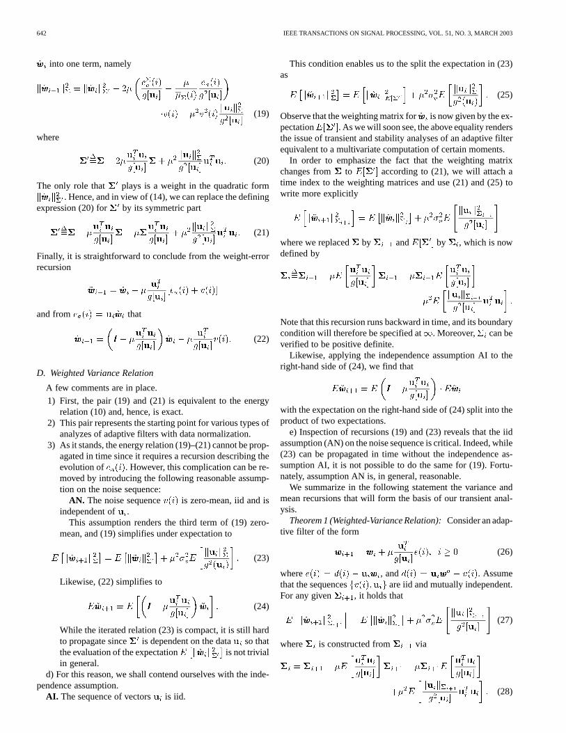
642 IEEE TRANSACTIONS ON SIGNAL PROCESSING, VOL. 51, NO. 3, MARCH 2003
into one term, namely
(19)
where
(20)
The only role that plays is a weight in the quadratic form. Hence, and in view of (14), we can replace the defining
expression (20) for by its symmetric part
(21)
Finally, it is straightforward to conclude from the weight-errorrecursion
and from that
(22)
D. Weighted Variance Relation
A few comments are in place.
1) First, the pair (19) and (21) is equivalent to the energyrelation (10) and, hence, is exact.
2) This pair represents the starting point for various types ofanalyzes of adaptive filters with data normalization.
3) As it stands, the energy relation (19)–(21) cannot be prop-agated in time since it requires a recursion describing theevolution of . However, this complication can be re-moved by introducing the following reasonable assump-tion on the noise sequence:
AN. The noise sequence is zero-mean, iid and isindependent of .
This assumption renders the third term of (19) zero-mean, and (19) simplifies under expectation to
(23)
Likewise, (22) simplifies to
(24)
While the iterated relation (23) is compact, it is still hardto propagate since is dependent on the data so thatthe evaluation of the expectation is not trivialin general.
d) For this reason, we shall contend ourselves with the inde-pendence assumption.
AI. The sequence of vectors is iid.
This condition enables us to the split the expectation in (23)as
(25)
Observe that the weighting matrix for is now given by the ex-pectation . As we will soon see, the above equality rendersthe issue of transient and stability analyses of an adaptive filterequivalent to a multivariate computation of certain moments.
In order to emphasize the fact that the weighting matrixchanges from to according to (21), we will attach atime index to the weighting matrices and use (21) and (25) towrite more explicitly
where we replaced by and by , which is nowdefined by
Note that this recursion runs backward in time, and its boundarycondition will therefore be specified at . Moreover, can beverified to be positive definite.
Likewise, applying the independence assumption AI to theright-hand side of (24), we find that
with the expectation on the right-hand side of (24) split into theproduct of two expectations.
e) Inspection of recursions (19) and (23) reveals that the iidassumption (AN) on the noise sequence is critical. Indeed, while(23) can be propagated in time without the independence as-sumption AI, it is not possible to do the same for (19). Fortu-nately, assumption AN is, in general, reasonable.
We summarize in the following statement the variance andmean recursions that will form the basis of our transient anal-ysis.
Theorem 1 (Weighted-Variance Relation):Consider an adap-tive filter of the form
(26)
where , and . Assumethat the sequences are iid and mutually independent.For any given , it holds that
(27)
where is constructed from via
(28)

AL-NAFFOURI AND SAYED: TRANSIENT ANALYSIS OF DATA-NORMALIZED ADAPTIVE FILTERS 643
It also holds that the mean weight-error vector satisfies
(29)
The purpose of the sections that follow is to show how theabove variance and mean recursions can be used to study thetransient performance of adaptive schemes with data nonlinear-ities. In particular, we will show how the freedom in selectingthe weighting matrix can be used advantageously to de-rive several performance measures.
First, however, we shall illustrate the mechanism of our anal-ysisbyconsidering twospecialcasesforwhichresultsarealreadyavailable in the literature.Morespecifically, we will start with thetransient analysis of LMS and normalized LMS algorithms forGaussian regression data in Sections III and IV. Once the mainideas have been illustrated in this manner, we will then describeour general procedure in Section V, which applies to adaptive fil-ters with more general data normalizations, as well as to regres-sion data that are not restricted to being Gaussian or white.
E. Change of Variables
In the meantime, we remark that sometimes it is useful toemploy a convenient change of coordinates, especially whendealing with Gaussian regressors. Thus, let denotethe covariance matrix of and introduce its eigendecomposi-tion
where is orthogonal, and is a positive diagonal matrix withentries . Define further
(30)
In view of the orthogonal transformation property (13), we have
and
Moreover, assuming that the nonlinearity is invariant underorthogonal transformations, i.e., (e.g.,or ), we find that the variance relation (27) retainsthe same form, namely
(31)
By premultiplying both sides of (28) by and post-multiplyingby , we similarly see that (28) also retains the same form
(32)
Likewise, (29) becomes
(33)
III. LMS W ITH GAUSSIAN REGRESSORS
Consider the LMS algorithm for which and assumethe following.
AG. The regressors arise from a Gaussian distributionwith covariance matrix .
In this case, the data dependent moments that appear in(31)–(33) are given by
Tr
Therefore, for LMS, recursions (31) and (32) simplify to
(34)
and
Tr (35)
while (33) becomes
(36)
Now, observe that in recursion (35), will be diagonal ifis. Therefore, in order for all successives to be diagonal
it is sufficient to assume that the boundary condition for therecursion for is taken as diagonal. In this way, thes will becompletely characterized by their diagonal entries. This promptsus to define the column vectors
diag and diag
In terms of these vectors, the matrix recursion (35) can be re-placed by the more compact vector recursion
or
(37)
where
The matrix describes the dynamics by which the weightingmatrices evolve in time, and its eigenstructure turns out tobe essential for filter stability. Using the fact that ,we can rewrite (34) using a compact vector weighting notation
(38)
Recursions (36)–(38) describe the transient behavior of LMS,and conclusions about mean-square stability and mean-squareperformance are now possible.
In transient analysis, we are interested in the time evo-lution of the expectations or, equivalently,
since and are related via the orthogonalmatrix . We start with the mean behavior.
A. Mean Behavior and Mean Stability
From (36) we find that the filter is convergent in the mean if,and only if, the step-size satisfies
(39)
where is the largest eigenvalue of.
B. Mean-Square Behavior
The evolution of can be deduced fromthe variance recursion (34) if is chosen as (or,

644 IEEE TRANSACTIONS ON SIGNAL PROCESSING, VOL. 51, NO. 3, MARCH 2003
equivalently, ). This corresponds to choosing in(38) as a column vector with unit entries, which is denoted by
Now, we can see from (38) that
(40)
which shows that in order to evaluate , we needwith a weighting matrix equal to . Now,
can be deduced from (38) by setting ,i.e.,
(41)
Again, in order to evaluate , we need
with weighting . This term can be deduced from (38) bychoosing
(42)
and a new term with weighting matrix appears. Fortunately,this procedure terminates in view of the Cayley–Hamilton the-orem. Thus, let denote the characteristicpolynomial of ; it is an th-order polynomial in
with coefficients . The Cayley–Hamilton theoremstates that every matrix satisfies its characteristic equation, i.e.,
, which allows us to conclude that
(43)
We can now collect the above results into a single recursion bywriting (40)–(43) as
......
... ...
If we define the vector and matrix quantities as indi-cated above, then the recursion can be rewritten more compactlyas
(44)
We therefore find that the transient behavior of LMS is de-scribed by the -dimensional state-space recursion (44) with
coefficient matrix .1 The evolution of the top entry of cor-responds to the mean-square deviation of the filter. Observe fur-ther that the eigenvalues of coincide with those of .
It is worth remarking that the same derivation that led to (44)with defined in terms of the unity vectorcan be repeatedfor any other choice of , say for some , toconclude that the same recursion (44) still holds withreplacedby . For instance, if we choose , then the top entry of theresulting state vector will correspond to the learning curveof the adaptive filter. In Section V-B we will use this remarkto describe more fully the learning behavior of adaptive filterswith data normalizations.
C. Mean-Square Stability
From the results in the above two sections, we conclude thatthe LMS filter will be stable in the mean and mean-square sensesif, and only if, satisfies (39) and guarantees the stability ofthe matrix (i.e., all the eigenvalues of should lie inside theunit circle). Since is easily seen to be non-negative definitein this case, we only need to worry about guaranteeing that itseigenvalues be smaller than unity.
Let us write in the form
where the matrices and are both positive-definite and givenby
(45)
It follows from the argument in Appendix A that the eigenvaluesof will be upper bounded by one if, and only if, the parameter
satisfies
(46)
in terms of the maximum eigenvalue of (all eigenvaluesof are real and positive). The above upper bound oncanalso be interpreted as the smallest positive scalarthat makes
singular. Let us denote this value ofby .Combining (46) with (39), we find that should satisfy
We can be more specific about and show that it is smallerthan . Actually, we can characterize in terms ofthe eigenvalues of as follows. Using the definitions (45) for
and , it can be verified that for all
The values of that result inshould therefore satisfy
1To be more precise, the transient behavior of LMS is described by the com-bination of both (44) and recursion (36).

AL-NAFFOURI AND SAYED: TRANSIENT ANALYSIS OF DATA-NORMALIZED ADAPTIVE FILTERS 645
i.e.,
This equality has a unique solution inside the interval. This is because the function
is monotonically increasing in the interval . More-over, it evaluates to 0 at and becomes unbounded as
. We therefore conclude that LMS is stable in themean- and mean-square senses for all step sizessatisfying
D. Steady-State Performance
Once filter stability has been guaranteed, we can proceed toderive expressions for the steady-state value of the mean-squareerror (MSE) and the mean-square deviation (MSD). To this end,note that in steady state, we have that for any vector
Thus, in the limit, (38) leads to
(47)
Here, diag denotes the boundary condition of therecursion (32), which we are free to choose.
Now, in order to evaluate the MSE, we first recall that it isdefined by
MSE
which, in view of the independence assumption AI, is also givenby
MSE
This is because
Therefore, to obtain the MSE, we should choose in (47) sothat , in which case, we get
MSE (48)
A more explicit expression for the MSE can be obtained byusing the matrix inversion lemma to evaluate the matrix inversethat appears in (48). Doing so leads to the well-known result
MSE
The MSD can be calculated along the same lines by noting that
MSD
The above means that in order to obtain an expression forthe MSD, we should now choose in (47) such that
, which yields
MSD
Just like the expression for the MSE, we can use the matrixinversion lemma to get an explicit expression forand, subsequently, for the MSD
MSD
Both of these steady-state expressions were derived in [5]. Here,we arrived at the expressions as a byproduct of a framework thatcan also handle a variety of data-normalized adaptive filters (seeSection V). In addition, observe how the expressions for MSEand MSD can be obtained simply by conveniently choosing dif-ferent values for the boundary condition .
IV. NORMALIZED LMS WITH GAUSSIAN REGRESSORS
We now consider the normalized LMS algorithm, for whichwith . For this choice of , recur-
sion (32) becomes
(49)
Progress in the analysis is now pending on the evaluation of themoments
(50)
Although the individual elements of are independent, noclosed-form expressions for and are available. However,we can carry out the analysis in terms of these matrices asfollows. First, we argue in Appendix B that is diagonal. Wealso show that if is diagonal, then so is and that
diag diag
where is the diagonal matrix
Here, the notation denotes an element-by-element(Hadamard) product.2 Thus, the successive s in recur-sion (49) will also be diagonal if the boundary condition is.Subsequently, as in the LMS case, we can again obtain a recur-sive relation for their diagonal entries of the form ,where retains the same form, namely
Mean-square stability now requires that the step-sizebechosen such that is a stable matrix (i.e., all its eigenvaluesshould be strictly inside the unit circle). For NLMS, it can be
2For two row vectorsfx;yg, the quantityx � y is a row vector with theelementwise products; see [24].

646 IEEE TRANSACTIONS ON SIGNAL PROCESSING, VOL. 51, NO. 3, MARCH 2003
verified that is a sufficient condition for this fact to hold,as can be seen from the following argument.
Choosing , we have
and
Obviously, so that
and, hence
Now, it is clear that . Moreover, over theinterval , it holds that
from which we conclude that
where the scalar coefficient is positive and strictly less thanone for . It follows that remains boundedfor all , as desired. It is also straightforward to verify from
that guarantees filter stability in the mean as well (justnote that is a rank-one matrix whose largesteigenvalue is smaller than one).
Finally, repeating the discussion we had for the steady-stateperformance of LMS, we arrive at the following expressions forthe MSE and MSD of normalized LMS:
MSE
MSD
These expressions hold for arbitrary colored Gaussian regres-sors.
The presentation so far illustrates how the energy-conserva-tion approach can be used to perform transient analysis of LMSand its normalized version. Our contribution lies in the abilityto perform the analysis in a unified manner. This can be ap-preciated, for example, by comparing the analysis of the nor-malized LMS algorithm in [7], [10], [11], [22], and [23] withthe analysis in the previous section. A substantial part of priorstudies is often devoted to studying the multivariate momentsof (50) and, as a result, eventually resort to some whiteness as-sumption on the data. Our derivation bypasses this requirement.
Moreover, earlier approaches do not seem to handle transpar-ently non-Gaussian regression data, which is discussed later inSection V.
V. DATA-NORMALIZED FILTERS
We now consider general data-normalized adaptive filters ofthe form (26) and drop the Gaussian assumption AG. The anal-ysis that follows shows how to extend the discussions of theprevious two sections to this general scenario.
Our starting point is the mean and variance relations(27)–(29).
A. Mean-Square Analysis
For arbitrary regression data, we can no longer guarantee thatthe data moments
are jointly diagonalizable (as we had, for example, in the caseof LMS with Gaussian regressors). Consequently,need notbe diagonal even if is, i.e., these matrices can no more befully characterized by their diagonal elements alone. Still, wecan perform mean-square analysis by replacing the diag oper-ation with the vec operation, which transforms a matrix into acolumn vector by stacking all its columns on top of each other.
Let
vec
Then, using the Kronecker product notation (e.g., [24]) and thefollowing property, for arbitrary matrices :
vec vec
it is straightforward to verify that the recursion (28) for trans-forms into the linear vector relation
where the coefficient matrix is now and is givenby
(51)
with the symmetric matrices defined by
In particular, is positive-definite, and is non-negative-def-inite. In addition, introduce the matrix
which appears in the mean weight-error recursion (29) and inthe expression for .
It follows that in terms of the vec notation, the variance rela-tion (27) becomes
(52)

AL-NAFFOURI AND SAYED: TRANSIENT ANALYSIS OF DATA-NORMALIZED ADAPTIVE FILTERS 647
Now, contrary to the Gaussian LMS case, the matrixis nolonger guaranteed to be non-negative-definite. It is shown inAppendix A that the condition can be enforcedfor values of in the range
(53)
where the second condition is in terms of the largest positivereal eigenvalue of the following block matrix:
when it exists. Since is not symmetric, its eigenvalues maynot be positive or even real. If does not have any real positiveeigenvalue, then the corresponding condition is removed from(53), and we only require . Condition (53)can be grouped together with the requirement ,which guarantees convergence in the mean, so that
(54)Moreover, the same argument that we used in the LMS casein Section III would show that the transient behavior of data-normalized filters is characterized by the -dimensional state-space model:3
(55)
where
...
with
denoting the characteristic polynomial of. In addition, andare the 1 vectors
...
...
3Observe how the order of the model, in the general case, isM and notM ,as was the case in the previous two sections with Gaussian regressors.
for any of interest, e.g., more commonly, or ,where vec .
Moreover, steady-state analysis can be carried out along thesame lines of Section III-D. Thus, assuming the filter reachessteady-state, recursion (52) becomes, in the limit
in terms of the boundary condition , which we arefree to choose. This expression allows us to evaluate thesteady-state value of for any symmetric weighting
by choosing such that vec . Inparticular, the EMSE corresponds to the choice , i.e.,
vec . Likewise, the MSD is obtained bychoosing , i.e., vec . We summarizethese results in the following statement, which holds forarbitrary input distributions and scalar data nonlinearities.
We summarize in the following statement the above results,which hold for arbitrary input distributions and data nonlinear-ities.
Theorem 2 (Scalar Nonlinearities):Consider an adaptivefilter of the form
where , and . Assumethat the sequences are iid and mutually independent.Then, the filter is stable in the mean and mean-square senses ifthe step-size satisfies (54). Moreover, the resulting EMSE andMSD are given by
EMSEvec
MSDvec
where is defined by (51).
B. Learning Curves
The learning curve of an adaptive filter refers to the time evo-lution of ; its steady-state value is the MSE. Now, since
, the learning curve can be evaluated by com-puting for each . This task can be accomplished re-cursively from (52) by choosing the boundary conditionas vec . Indeed, iterating (52) with this choice ofand assuming , we find that
that is
where the vector and the scalar satisfy the recursions

648 IEEE TRANSACTIONS ON SIGNAL PROCESSING, VOL. 51, NO. 3, MARCH 2003
Using these definitions for , it is easy to verify that
which describes the learning curve of a data-normalized adap-tive filter.
VI. M ATRIX NONLINEARITIES
In this section, we extend the earlier results to the case inwhich the function is matrix-valued rather than scalar-valued. To motivate this extension, consider the sign-regressoralgorithm (e.g., [8]):
sgn
where the sgn operates on the individual elements of. Thisis in contrast to the discussions in the previous sections whereall the elements of were normalized by the same data non-linearity. Other examples of matrix nonlinearities can be found,e.g., in [25]–[27].
The above update is a special case of more general updatesof the form
(56)
where denotes an matrix nonlinearity.
A. Energy Relation
We first show how to extend the energy relation of Theorem1 to the more general class of algorithms (56) with matrix datanonlinearities. Our starting point is the adaptation equations(56), which can be written in terms of the weight error vector
as
(57)
By premultiplying both sides of (57) by , we see that theestimation errors , , and are related by
(58)
Moreover, the two sides of (57) should have the same weighted-energy, i.e.,
so that
(59)
This form of the energy relation is analogous to (15). As itstands, (59) is just what we need for mean-square analysis. Forcompleteness, however, we develop a cleaner form of (59): aform similar to (10). To this end, notice that upon replacingby in (58), we get
or, by incorporating the defining expression (9) of
(60)
Substituting (60) into (59) produces the desired energy relationform
B. Mean-Square Analysis
To perform mean-square analysis, we start with form (59) ofthe energy relation. Bearing in mind the independence assump-tion on the noise AN and the fact that , (59)reads, under expectation
where the weight was replaced by the time-indexed weight. If we further invoke the polarization identity (12), we get
and
These equations, together with the linearity property (11) andthe independence assumption AI, yield the following result.
Theorem 3 (Matrix Nonlinearities):Consider an adaptivefilter of the form
where , and . Assumethat the sequences are iid and mutually independent.Then, it holds that
(61)
where
(62)
In addition, the stability condition and the MSE and MSD ex-pressions of Theorem 2 apply here as well with replacedby
Moreover, the construction of the learning curve in Section V-Balso extends to this case.
Compared with some earlier studies (e.g., [8], [9], [25]), theabove results hold without restricting the regression data tobeing Gaussian or white.
C. Sign-Regressor Algorithm
To illustrate the application of the above results, we return tothe sign-regressor recursion
sgn

AL-NAFFOURI AND SAYED: TRANSIENT ANALYSIS OF DATA-NORMALIZED ADAPTIVE FILTERS 649
Fig. 1. Theoretical and simulated learning and MSD curves for LMS using correlated uniform input data anda = 0:2.
In this case, the matrix nonlinearity is implicitly definedby the identity
sgn
which in turn means that relations (61) and (62) become
sgn (63)
and
sgn sgn
sgn
Assume that the individual entries of the regressorhave vari-ance . In addition, assume that has a Gaussian distribution.Then, it follows from Price’s theorem [29] that4
sgn
which leads to
sgn (64)
Now, observe thatsgn Tr wheneveris diagonal. Thus, assume we choose . Then, the ex-pression for becomes
4The theorem can be used to show that for two jointly zero-meanGaussian real-valued random variablesx andy, it holds thatE (xsgn(y)) =2=�1=� E (xy).
whereas (63) becomes
(65)
It is now easy to verify that converges, provided thator, equivalently
This is the same condition derived in [8].To evaluate the MSE, we observe from (65) that in steady
state
so that
MSE
which is again the same expression from [8].
VII. SIMULATIONS
Throughout this section, the system to be identified is an FIRchannel of length 4. The input is generated by passing aniid uniform process through a first-order model
(66)
By varying the value of , we obtain processes of differentcolors. We simulate the choices and . The inputsequence that is feeding the adaptive filter therefore has a corre-lated uniform distribution. The output of the channel is contami-nated by an iid Gaussian additive noise at an SNR level of 30 dB.
Figs. 1 and 2 shows the resulting theoretical and simulatedlearning and MSD curves for both cases of and

650 IEEE TRANSACTIONS ON SIGNAL PROCESSING, VOL. 51, NO. 3, MARCH 2003
Fig. 2. Theoretical and simulated learning curves for LMS using correlated uniform input data anda = 0:9.
Fig. 3. Theoretical and simulated EMSE for LMS as a function of the step-size for correlated uniform input witha = 0:2.
. The simulated curves are obtained by averaging over 200experiments, whereas the theoretical curves are obtained fromthe state-space model (55). It is seen that there is a good matchbetween theory and practice.
Fig. 3 examines the stability bound (54); it plots the filterEMSE as a function of the step size using the theoretical ex-pression from Theorem 2, in addition to a simulated EMSE. Thebound on the step size is also indicated.
VIII. C ONCLUDING REMARKS
In this paper, we developed a framework for the transientanalysis of adaptive filters with general data nonlinearities(both scalar-valued and matrix-valued). The approach relieson energy conservation arguments. By suitably choosing theboundary condition of the weighting matrix recursion, wecan obtain MSE and MSD results and the conditions formean-square stability. We may add that extensions to leakyalgorithms, affine projection algorithms, filters with error
nonlinearities, and to tracking analysis are possible and aretreated in, e.g., [20], [30], and [31].
APPENDIX ACONDITION FOR MEAN-SQUARE STABILITY
Consider the matrix form with ,, and . We would like to determine conditions on
in order to guarantee that the eigenvalues ofsatisfy.
First, in order to guarantee , the step-size shouldbe such that or, equivalently, . This conditionis equivalent to requiring , but sincethe matrices and are similar, we concludethat should satisfy .
In order to enforce , the step-size should besuch that When , theeigenvalues of are positive and equal to 2. As increases,the eigenvalues of vary continuously with . Therefore, an

AL-NAFFOURI AND SAYED: TRANSIENT ANALYSIS OF DATA-NORMALIZED ADAPTIVE FILTERS 651
upper bound on that guarantees is determined bythe smallest that makes singular.
Now, the determinant of is equal to the determinant ofthe block matrix
Moreover, since
the condition is equivalent to ,where
In this way, the smallest positivethat results inis given by
This condition is in terms of the largest positive real eigenvalueof when it exists. It follows that the following range ofguarantees a stable,
APPENDIX BAND OF (50) ARE DIAGONAL
An off-diagonal entry of has the form
Now, is an odd function of , which hasan even (Gaussian) pdf and is independent of the other elementsof . Thus, , and hence, iszero as well. Therefore, is diagonal. A similar argument canbe used to prove that is diagonal. Now, a diagonal entry of
can be written as
diag
It follows that
diag diag
where
ACKNOWLEDGMENT
The authors are grateful to Dr. V. H. Nascimento for his as-sistance with the material in Appendix A.
REFERENCES
[1] B. Widrow and S. D. Stearns,Adaptive Signal Processing. EnglewoodCliffs, NJ: Prentice-Hall, 1985.
[2] S. Haykin,Adaptive Filter Theory, 3rd ed. Englewood Cliffs, NJ: Pren-tice-Hall, 1996.
[3] O. Macchi,Adaptive Processing: The LMS Approach with Applicationsin Transmission. New York: Wiley, 1995.
[4] S. K. Jones, R. K. Cavin, and W. M. Reed, “Analysis of error-gradientadaptive linear estimators for a class of stationary dependent processes,”IEEE Trans. Inform. Theory, vol. IT-28, pp. 318–329, Mar. 1982.
[5] A. Feuer and E. Weinstein, “Convergence analysis of LMS filters withuncorrelated Gaussian data,”IEEE Trans. Acoust., Speech, Signal Pro-cessing, vol. ASSP-33, Jan. 1985.
[6] V. Mathews and S. Cho, “Improved convergence analysis of stochasticgradient adaptive filters using the sign algorithm,”IEEE Trans. Acoust.,Speech, Signal Processing, vol. ASSP–35, pp. 450–454, Apr. 1987.
[7] M. Tarrab and A. Feuer, “Convergence and performance analysis ofthe normalized LMS algorithm with uncorrelated Gaussian data,”IEEETrans. Inform. Theory, vol. 34, pp. 680–690, July 1988.
[8] E. Eweda, “Analysis and design of signed regressor LMS algo-rithm for stationary and nonstationary adaptive filtering withcorrelated Gaussian data,”IEEE Trans. Circuits Syst., vol. 37, pp.1367–1374, Nov. 1990.
[9] S. C. Douglas and T. H. -Y. Meng, “The optimum scalar data nonlin-earity in LMS adaptation for arbitrary iid inputs,”IEEE Trans. SignalProcessing, vol. 40, pp. 1566–1570, June 1992.
[10] M. Rupp, “The behavior of LMS and NLMS algorithms in the presenceof spherically invariant processes,”IEEE Trans. Signal Processing, vol.41, pp. 1149–1160, Mar. 1993.
[11] D. T. M. Slock, “On the convergence behavior of the LMS and the nor-malized LMS algorithms,”IEEE Trans. Signal Processing, vol. 41, pp.2811–2825, Sept. 1993.
[12] J. Mai and A. H. Sayed, “A feedback approach to the steady-state per-formance of fractionally-spaced blind adaptive equalizers,”IEEE Trans.Signal Processing, vol. 48, pp. 80–91, Jan. 2000.
[13] N. R. Yousef and A. H. Sayed, “A unified approach to the steady-stateand tracking analyzes of adaptive filters,”IEEE Trans. Signal Pro-cessing, vol. 49, pp. 314–324, Feb. 2001.
[14] , “Ability of adaptive filters to track carrier offsets and randomchannel nonstationarities,”IEEE Trans. Signal Processing, vol. 50, pp.1533–1544, July 2002.
[15] , “A feedback analysis of the tracking performance of blind adap-tive equalization algorithms,” inProc. Conf. Decision Contr., vol. 1,Phoenix, AZ, Dec. 1999, pp. 174–179.
[16] A. H. Sayed and M. Rupp, “A time-domain feedback analysis of adap-tive algorithms via the small gain theorem,” inProc. SPIE, vol. 2563,San Diego, CA, July 1995, pp. 458–69.
[17] M. Rupp and A. H. Sayed, “A time-domain feedback analysis of filtered-error adaptive gradient algorithms,”IEEE Trans. Signal Processing, vol.44, pp. 1428–1439, June 1996.
[18] A. H. Sayed and M. Rupp, “Robustness issues in adaptive filtering,” inDSP Handbook. Boca Raton, FL: CRC, 1998, ch. 20.
[19] M. Rupp and A. H. Sayed, “On the convergence of blind adaptive equal-izers for constant-modulus signals,”IEEE Trans. Communications, vol.48, pp. 795–803, May 2000.
[20] T. Y. Al-Naffouri and A. H. Sayed, “Transient analysis of adaptive filterswith error nonlinearities,”IEEE Trans. Signal Processing, vol. 51, pp.653–663, Mar. 2002.
[21] B. Widrow, J. McCool, M. G. Larimore, and C. R. Johnson, “Stationaryand nonstationary learning characteristics of the LMS adaptive filter,”Proc. IEEE, vol. 46, pp. 1151–1162, Aug. 1976.
[22] N. J. Bershad, “Behavior of the�-normalized LMS algorithm withGaussian inputs,”IEEE Trans. Acoust., Speech, Signal Processing, vol.ASSP–35, pp. 636–644, May 1987.
[23] , “Analysis of the normalized LMS algorithm with Gaussian in-puts,”IEEE Trans. Acoust. Speech Signal Processing, vol. ASSP-34, pp.793–806, 1986.
[24] H. Lütkepohl,Handbook of Matrices. New York: Wiley, 1996.[25] N. J. Bershad, “On the optimum data nonlinearity in LMS adaptation,”
IEEE Trans. Acoust., Speech, Signal Processing, vol. ASSP-34, pp.69–76, Feb. 1986.
[26] W. B. Mikhaelet al., “Adaptive filters with individual adaptation of pa-rameters,”IEEE Trans. Circuits Syst., vol. CAS–33, July 1986.
[27] R. W. Harris, D. M. Chabries, and F. A. Bishop, “A variable step (VS)adaptive filter algorithm,”IEEE Trans. Acoust., Speech, Signal Pro-cessing, vol. ASSP-34, pp. 309–316, Apr. 1986.

652 IEEE TRANSACTIONS ON SIGNAL PROCESSING, VOL. 51, NO. 3, MARCH 2003
[28] S. C. Douglas and T. H. -Y. Meng, “Normalized data nonlinearitiesfor LMS adaptation,” IEEE Trans. Signal Processing, vol. 42, pp.1352–1365, June 1994.
[29] R. Price, “A useful theorem for nonlinear devices having Gaussian in-puts,” IRE Trans. Inform. Theory, vol. IT-4, pp. 69–72, June 1958.
[30] A. H. Sayed and T. Y. Al-Naffouri, “Mean-square analysis of normalizedleaky adaptive filters,” inProc. ICASSP, vol. VI, Salt Lake City, UT,May 2001.
[31] H.-C. Shin and A. H. Sayed, “Transient behavior of affine projectionalgorithms,” inProc. ICASSP, Hong Kong, Apr. 2003, to be published.
Tareq Y. Al-Naffouri received the B.S. degree inmathematics (with honors) and the M.S. degree inelectrical engineering from King Fahd Universityof Petroleum and Minerals, Dhahran, Saudi Arabia,in 1994 and 1997, respectively, and the M.S. degreein electrical engineering from Georgia Instituteof Technology, Atlanta, in 1998. He is currentlypursuing the Ph.D. degree with the Electrical Engi-neering Department, Stanford University, Stanford,CA.
His research interests lie in the area of signal pro-cessing for communications. Specifically, he is interested in the analysis anddesign of algorithms for channel identification and equalization. He has heldinternship positions at NEC Research Labs, Tokyo, Japan, and at National Semi-conductor, Santa Clara, CA.
Mr. Al-Naffouri is the recipient of a 2001 best student paper award at aninternational meeting for work on adaptive filtering analysis.
Ali H. Sayed (F’01) received the Ph.D. degreein electrical engineering in 1992 from StanfordUniversity, Stanford, CA.
He is currently Professor and Vice-Chair ofelectrical engineering at the University of California,Los Angeles. He is also the Principal Investi-gator of the UCLA Adaptive Systems Laboratory(www.ee.ucla.edu/asl). He has over 180 journaland conference publications, is the author of theforthcoming textbookFundamentals of AdaptiveFiltering (New York: Wiley, 2003), is coauthor
of the research monographIndefinite Quadratic Estimation and Control(Philadelphia, PA: SIAM, 1999) and of the graduate-level textbookLinearEstimation(Englewood Cliffs, NJ: Prentice-Hall, 2000). He is also co-editor ofthe volumeFast Reliable Algorithms for Matrices with Structure(Philadelphia,PA: SIAM, 1999). He is a member of the editorial boards of theSIAM Journalon Matrix Analysis and Its Applicationsand the International Journal ofAdaptive Control and Signal Processingand has served as coeditor of specialissues of the journalLinear Algebra and Its Applications. He has contributedseveral articles to engineering and mathematical encyclopedias and handbooksand has served on the program committees of several international meetings.He has also consulted with industry in the areas of adaptive filtering, adaptiveequalization, and echo cancellation. His research interests span several areasincluding adaptive and statistical signal processing, filtering and estimationtheories, signal processing for communications, interplays between signalprocessing and control methodologies, system theory, and fast algorithms forlarge-scale problems.
Dr. Sayed is recipient of the 1996 IEEE Donald G. Fink Award, a 2002 BestPaper Award from the IEEE Signal Processing Society in the area of SignalProcesing Theory and Methods, and co-author of two Best Student Paper awardsat international meetings. He is also a member of the technical committees onSignal Processing Theory and Methods (SPTM) and on Signal Processing forCommunications (SPCOM), both of the IEEE Signal Processing Society. He is amember of the editorial board of the IEEE SIGNAL PROCESSINGMAGAZINE. Hehas also served twice as Associate Editor of the IEEE TRANSACTIONS ONSIGNAL
PROCESSINGand is now serving as Editor-in-Chief of the TRANSACTIONS.