Block implementation of adaptive digital filters

744 IEEE TRANSACTIONS ON ACOUSTICS, SPEECH, AND SIGNAL PROCESSING, VOL. ASSP-29, NO. 3, JUNE 1981

(b)K., Martin, ‘‘@proved circuits for the realization of switched- capacitor filters, IEEE Trans. Cirnu’ts Syst., vol. CAS-27, pp. 237-244, Apr. 1980,

ogies for analog integrated circuits,” IEEE J . Solid-State Circuits, D. Hodges, P. Gray, and R. Brodersen, “Potential of MOS technol-

vol. SC-13, pp. 285-293, June 1978. G. Temes, H. Orchard, and M. Jahanbegloo, “Switched-capacitor

Syst., vol. CAS-12, pp. 1039-1044, Dec. 1978. filter design using the bilinear z-transform,” ZEEE Trans. Circuits

K. Martin and A. Sedra, “Strays-insensitive switched capacitor filters based on the bilinear z-transform,” Electron. Lett., vol. 15, no. 13, pp. 365-366, June 1979. B. White, G. Jacobs, and G. Landsburg, “A monolithic dual tone

pp. 991-997, Dec. 1979. multifrequency receiver,” ZEEE J . Solid-State Circuits, vol. SC-14,

P. Fleischer and K. Laker, “A family of active switched capacitor biquad building blocks,” Bell Syst. Tech. J., vol. 58, pp. 2235-2269, Dec. 1979. K. Martin and A. Sedra, “Exact design of switched-capacitor band- pass filters using coupled-biquad structures,” ZEEE Trans. Circuits Syst., vol. 27, pp. 469-475, June 1980.

coupled device (CCD) adaptive discrete analog signal processing,” M. White, I. Mack, G. Barsuk, D. Lamps, and F. Kub, “Charge-

IEEE J . Solid-State Circuits, vol. SC-14, pp. 132- 147, Feb. 1979. B. Ahuja, M. Copeland, and C. Y. Chan, “A sampled analog MOS LSI adaptive filter,” IEEE J . Solid-State Circuits, vol. SC-14, pp. 148-154. Feb. 1979. H.-Kho&amabadi, “NMOS phase lock loop,” University of Cali-

T. Foxall, R. Whitbread, L. Sellars, A. Aitken, and J. Morris, “A fornia Berkeley, Int. Memo. UCB/ERL M77/67, Nov. 1977.

switched capacitor bandsplit filter using double polysilicon oxide isolated CMOS,” 1980 ISSCC, Dig. of Tech. Pap., pp. 90-91, Feb. 1980. D.-Allstot, R. Brodersen, and P. Gray, “An electrically programma- ble analog NMOS second order filter,” 1979 ISSCC Dig. Tech. Pap. pp. 76-88, Feb. 1979. A. Grebene. Analoa Integrated Circuit Desian. New York: Van Nostrand Reinholdypp. 210-238, 1972. Y. Chen and D. Duttweiler, “A 35 000-transistor chip VLSI echo canceller,” 1980 ISSCC Dig. Tech. Pap., pp. 42-43, Feb. 1980.

-

Ken Martin (S’73-M77) was born in Hamilton, Ont., Canada, in 1952. He received the B.A.Sc. (Hons.), M.A.Sc., and Ph.D. degrees from the University of Toronto, Toronto, Canada, in 1975, 1977 and 1980, all in electrical engineering.

From 1977 to 1978 he was a member of the Scientific Research Staff at Bell Northern Re- search, Ottawa, Ont., Canada. Since September 1980 he has been an Assistant Professor in the Department of Electrical Engineering, University of California, Los Angeles. He is also an in-

dustrial consultant. His research interests include active networks, filter design and digital signal processing. He has published a number of papers and holds a patent on the strays-insensitive inverting switched-capacitor integrator.

r)

Adel S. Sedra (”66) was born in Egypt, on November 2, 1943. He received the B.Sc. degree from Cairo University, Cairo. Egypt, in 1964, and the M.A.Sc. and Ph.D. degrees from the University of Toronto, Toronto, Ont., Canada, in 1968 and 1969, respectively, all in electrical engineering.

From 1964 to 1966, he served as Instructor and Research Engineer at Cairo University. He has been on the staff of the University of Toronto since 1969 and is currently Professor of Electrical

Engineering. He has also served as a Consultant to various industrial and government agencies in Canada and U.S.A. Since 1972 he has been Director and is currently President of Electrical Engineering Consociates Ltd., a research and design consulting firm. He has published about seventy technical articles and one book.

Block Implementation of Adaptive Digital Filters

Abstract-Block digital filtering involves the calculation of a block or finite set of filter outputs from a block of input values. This paper presents a block adaptive filtering procedure in which the filter coefficients are adjusted once per each output block in accordance with a generalized least mean-square (LMS) algorithm. Analyses of convergence properties and

work was su ported by the US . Department of Energy, Lawrence Manuscript received May 27, 1980; revised November 29, 1980. This

Livermore LaEoratory, Livermore, CA, under Contract W-7405-ENG-48. G. A. Clark is with the Electronics Engineering Department, Lawrence

Livermore Laboratory, Livermore, CA 94550. S . K. Mitra is with the Department of Electrical and Computer

Engineering, University of California, Santa Barbara, CA 93106. S . R. Parker is with the Department of Electrical Engineering, Naval

Postgraduate School, Monterey, CA 93940.

computational complexiQ show that the block adaptive filter permits fast implementations while maintaining performance equivalent to that of the widely used LMS adaptive filter.

B I. INTRODUCTION

LOCK DIGITAL filtering has been discussed exten- sively by Burrus, Mitra, and others [1]-[4]. The tech-

nique involves calculation of a block or finite set of output values from a block of input values. Block implementations of digital filters allow efficient use of parallel processors, which can result in speed gains. Furthermore, efficient block algorithms such as the fast Fourier transform (FFT) can be used to advantage when impiementing filters on

0096-35 18/8 1/0600-0744$00.75 0 198 1 IEEE

CLARK et ul.: BLOCK IMPLEMENTATION OF DIGITAL FILTERS 145

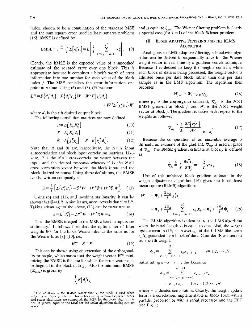
serial processors [5]-[7]. The continuing development of low-cost large-scale integrated circuits and parallel process- - ing architectures is likely to make block filtering increas- 'k

ingly attractive.

are modified and extended for use with nonrecursive least /

- - SIP

F,ilter W (Time or

frequency domain) PIS :

In this paper, the block processing techniques in [1]-[4] -- 7 - -

mean-square (LMS) adaptive filters [SI-[lo]. A block mean-square error (BMSE) performance criterion is defined, resulting in a BMSE gradient estimate that is a correlation (over a block of data) between the errors and the input signal. This gradient estimate leads to a weight adjustment algorithm that allows block implementation with either parallel processors or serial processors and the FFT. The computational complexity savings resulting from two block implementations are analyzed and shown to be substantial.

The adaptive digital filtering discussed here is of the LMS type presented by Widrow et af. [SI-[lo] for which the performance index is the mean-square error (MSE=(). All inputs are assumed to be real. The adaptive filter of Widrow is a finite impulse response (FIR) digital filter of order N - 1 for which the output yk at discrete time instant k is given as the convolution sum of the input xk and the filter weights wlk:

N yk= x w/kxk-/+I, k = 1 , 2 , 3 , . ' * . (1)

I= 1

The Widrow-Hoff LMS algorithm adjusts the filter weights in accordance with (2):

w k + l = w k +2pCkxk (2)

where p is the convergence constant, and Wk and x k are, respectively, the NX 1 weight vector and the NX 1 input vector:

w k A [ W l k w2k * ' . W N k I T

and c k is the error at the kth instant given by the difference between the desired output dk and the actual output yk, 1.e.,

This paper investigates the realization of adaptive filters by blockwise processing of the data in order to gain computational advantage. To use efficient block proce- dures, an adaptive algorithm must allow a whole block of outputs to be calculated without modifying the filter parameters. Thus a block adaptive filter should adjust the weights one per block of data. It is shown that the tradi- tional LMS adaptive filter, which adjusts parameters once' each data sample, is a special case of the block adaptive filter with a block length of one.

For the time-invariant case, (1) can be written in matrix form as

w - - c.

Block correlation operator and

- algorlthm (Time or 8

SIP we,ight update .

- frequency domain) - .c i -

Fig. 1 General block adaptive filterin configuration. S/P=serial-to- parallel converter. P/s=paralL-to-serid converter.

Letting L represent block length, the following low-order (L= 3, N = 3) example shows how this convolution is written in a convenient block form:

. I - - - - - - - --L I UL I I 7 - h

L J L ' J

In (5) the filter weights (rather than the inputs) are ex- pressed as a vector. This is contrary to the standard block processing formulation [ 11-[4], but makes block analysis convenient because it allows for simple differentiation with respect to the weights.

Using the block notation shown above, (2) can be written for the general ( L , N ) case as

5 = x .w I (6 ) where j is the block index, 5 and x are, respectively, the j t h output vector of length L, and the L X N matrix of input vectors:

A

'li = [ Y(j- 1)L+ 1 Y(j- 1)L+2 . Y j L ] T

This linear convolution can be implemented using a parallel processor or a serial processor and the FFT [5]-[7].

11. THE BLOCK WIENER FILTERING PROBLEM The classical Wiener filter can be extended to the block

input case as shown next. Refer to Fig. 1. Assuming that all inputs are stationary, let

A T dj [ d( j - 1)L+ 1 d(,- 1)L+2 * * *djL] (7)

be the L X 1 vector of desired responses for blockj, and let

be the L X 1 vector of errors for block j where Ck is defined in (3). The key element of this analysis is the performance


index, chosen to be a combination of the standard MSE and the sum square error used in least squares problems [16]. BMSE is defined by

" 1 j L BMSE=Z = ,"[ETE~]=E[ x c i ] . (9)

k=(j- l)L+ 1

Clearly, the BMSE is the expected value of a smoothed estimate of the squared error over one block. This is appropriate because it combines a block's worth of error information into one number for each value of the block index j. The MSE considers the error information one point at a time. Using (6) and ( 9 , (9) becomes

LZ = E { d,?d,} -E{ d , ? ~ , } W - W 'E{ x,TdJ}

+wTE(x,Tx;}w where dj is thejth desired'output block.

The following correlation matrices are now defined:

R=E[XkX:] ( 10)

P = E [ x, dk] (11)

$ = E [ X j ' X j ] , s = E [ x p , ] . (12)

Note that R and '3, are, respectively, the NXN input autocorrelation and block input correlation matrices. Like- wise, P is the NX 1 cross-correlation vector between the input and the desired response whereas 9 is the NX 1 cross-correlation vector between the block input and the block desired response. Using these definitions, the BMSE can be written compactly as

-- L c- [E{d:dj} --OTW- WrO+ WT%W]. (13)

Using (6) and (12), and invoking stationarity, it can be shown that 91,= LR. A similar argument reveals that O== LP. Taking advantage of the above, (13) can be re-written as

E = E [ d i ] - 2 P T W - W T R W = ( . (14)

Thus the BMSE is equal to the MSE when the inputs are stationary.' It follows then that the optimal set of filter weights W* for the block Wiener filter is the same as for the Wiener filter [8]-[ lo], i.e.,

W * = R - ' P . (15)

This can be shown using an extension of the orthogonal- ity principle, which states that the weight vector W* mini- mizing the BMSE is the one for which the error vector E, is orthogonal to the block data x j . Also the minimum BMSE (Zmin) is given by

L E [ 1 d p j ]

referring to block problems. This is because in Section IV, when block 'The notation Z for BMSE rather than 6 for MSE is used when

and scalar algorithms are compared, the MSE for the block algorithm is not, in general equal to the MSE for the scalar algorithm during convergence.

and is equal to tmin. The Wiener filtering problem is clearly a special case (for L= 1) of the block Wiener problem.

111. BLOCK ADAPTIVE FILTERING AND THE BLMS ALGORITHM

Analogous to LMS adaptive filtering, a blockwise algorithm can be derived to sequentially solve for the Wiener weight vector in real time by a gradient search technique. Because it is desired to keep the weights constant while each block of data is being processed, the weight vector is adjusted once per data block rather than one per data sample as in the LMS algorithm. The algorithm then becomes

? + I ? - p B V B ; (16) where p B is the convergence constant, v,, is the NX 1 BMSE gradient at block j , and ?. is the NX 1 weight vector at blockj. The gradient is taken with respect to the weights as follows:

Because the computation of an ensemble average is difficult, an estimate of the gradient, V B j , is used in place of vBj. The BMSE gradient estimate at block j is defined as

Use of this unbiased block gradient estimate in the weight adjustment algorithm (16) gives the block least mean square (BLMS) algorithm:

j L =T+% 2 E k X k = ? + + q . 2P (19)

k=(j- 1)L+ 1

The BLMS algorithm is identical to the LMS algorithm when the block length L is equal to one. Also, the weight update term in (1 9) is an average of the L LMS-like terms e k X, generated by a block of data. Consider aj written out for the i th weight:

iL +. . =

1 1 2 c k X k - i + , , i=1,2;. . , N . k = ( j - I ) L + 1

Substituting n=k-i+ 1, this becomes jL- - i+ 1

+ . .= 1J Z cn+i - lXn

n = ( j - I ) L - i + 2 - - e P j * x , , for i=1,2;- . ,N

where * indicates convolution. Clearly, the weight update term is a correlation, implementable in block form with a parallel processor or with a serial processor and the FFT (see Fig. 1).

CLARK et U/. : BLOCK IMPLEMENTATION OF DIGITAL FILTERS 747

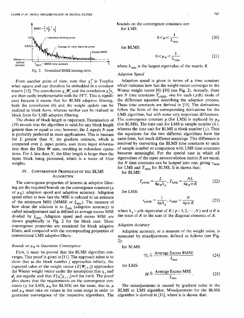
t Individual learning curve

Average of many learning curves

Wiener or optimal solution

Fig. 2. Normalized BMSE learning curve.

From another point of view, note that x ; is Toeplitz when square and can therefore be embedded in a circulant matrix [ 121. The convolution x,? and the correlation x?€. are then easily implementable with the FFT. This is sign[fL cant because it means that for BLMS adaptive filtering, both the convolution (6) and the weight update can be realized in block form, whereas neither can be realized in block form for LMS adaptive filtering.

The choice of block length is important. Examination of (19) reveals that the algorithm is valid for any block length greater than or equal to one; however, the L equals N case is probably preferred in most applications. This is because for L greater than N , the gradient estimate, which is computed over L input points, uses more input information than the filter W uses, resulting in redundant operations. For L less than N , the filter length is larger than the input block being processed, which is a waste of filter weights.

IV. CONVERGENCE PROPERTIES OF THE BLMS ALGORITHM

The convergence properties of interest in adaptive filtering are the required bounds on the convergence constant (p or p B ) , adaption speed and adaption accuracy. Adaption speed refers to how fast the MSE is reduced to an estimate of the minimum MSE (MMSE or Emin). The measure of how close the solution is to tmin (adaption accuracy) is called misadjustment and is defined as average excess MSE divided by Emin. Adaption speed and excess MSE are shown graphically in Fig. 2 for the block case. These convergence properties are examined for block adaptive filters, and compared with the corresponding properties of conventional LMS adaptive filters.

Bounds on p B to Guarantee Convergence First, it must be proved that the BLMS algorithm con-

verges. This proof is given in [ 1 11. The approach taken is to show that as the block number j approaches infinity, the expected value of the weight vector ( E [ y? , I ) approaches the Wiener weight vector under the assumptlon that x j and dj are ergodic and that E[x;xj+,]=O for l #O. The proof also shows that the requirements on the convergence constants (p for LMS, p B for BLMS) are the same, that is, p and p B must take on values in the same range in order to guarantee convergence of the respective algorithms. The

bounds on the convergence constants are: for LMS:

1 O<p<-

A max

for BLMS: 1

o<pLg<- A max

where Am, is the largest eigenvalue of the matrix R.

Adaption Speed Adaption speed is given in terms of a time constant

which indicates how fast the weight vector converges to the Wiener weight vector [8]-[ 101 (see Fig. 2). Actually, there are N time constants TpMSE, one, for each ( pth) mode of the difference equation describing the adaption process. These time constants are derived in [ll]. The derivations follow the form of the corresponding derivations for the LMS algorithm, but with some very important differences. The convergence constant p (for LMS) is replaced by p B (for BLMS). The time unit for LMS is sample number (k), whereas the time unit for BLMS is block number ( j ) . Thus the equations for the two different algorithms have the same form, but much different meanings. This difference is resolved by converting the BLMS time constants to units of sample number so comparison with LMS time constants becomes meaningful. For the special case in which all eigenvalues of the input autocorrelation matrix R are equal, the N time constants can be lumped into one, giving rMSE for LMS and TMSE for BLMS. It is shown that:

for BLMS:

for LMS:

where A, = p th eigenvalue of R ( p = 1,2,. . . , N ) and tr R is the trace of R or the sum of the diagonal elements of R.

Adaption Accuracy Adaption accuracy, or a measure of the weight noise, is

measured by misadjustment, defined as follows (see Fig. 2):

for BLMS: A Average Excess BMSE

%= (24) E min

for LMS: A Average Excess MSE M = (25)

Emin

The misadjustment is caused by gradient noise in the BLMS or LMS algorithm. Misadjustment for the BLMS algorithm is derived in [ll], where it is shown that:


for BLMS:

Average Excess BMSE = 7 tmin tr R , %= - tr R P B P B

L (26)

for LMS: Average Excess MSE = ptmin tr R , M = P tr R . (27)

Comparison of Concergence Properties for the LMS and BLMS Algorithms

Comparing the quantities presented above by taking ratios yields some interesting properties:

Thus it is observed that: The BLMS and LMS algorithms converge at the same

rate and achieve the same misadjustment if p B = L p . In using these relations for design purposes, one must

remember that p B and p have the same convergence bounds, because this fact limits the usable block length. For example, a possible situation is that p B = Lp and ,LL satisfies (20), but p and L are so large that (21) is not satisfied. This is less likely to occur, of course, for the case of slow adaption than for the case of fast adaption.

All the relations regarding BLMS convergence reduce to the LMS case when the block length L equals one.

Convergence Properties When Data is Correlated Adaptive filter performance equations are traditionally

derived assuming uncorrelated inputs because that is the case that is easily tractable. As discussed in [I 11, the convergence proof and derivations of convergence parameters for the BLMS algorithm are based on the assumption that the input matrices x and x j + ! are uncorrelated. For the LMS algorithm, the assumption 1s that X , and X, , , are uncorrelated. These assumptions lead to the assumptions that is independent of xi for the BLMS algorithm and Wk is independent of X , for the LMS algorithm. These assumptions simplify the proofs but are not appropriate for all data types. Both proofs also assume input stationarity.

References [ 131 and [ 141 discuss convergence properties when the data is correlated and present some results that strengthen arguments in favor of block adaptive filtering. Based upon the work of Gersho [15], Kim and Davisson use a sample average over a block of L data points to estimate the MSE gradient for adjusting the weights of an adaptive algorithm. They assume that the input data is M-dependent, which basically means that it is uncorrelated for autocorrelation lags greater than M (where M is a positive integer). Kim and Davisson show that when the inputs are M-dependent and the filter weights are adjusted once per block, the problems of analyzing convergence are overcome if L > ( M + N - - l), where N is the filter length and M is the M-dependence constant.

”2k

‘ lk dk - +

Model

1

Adaption algorithm

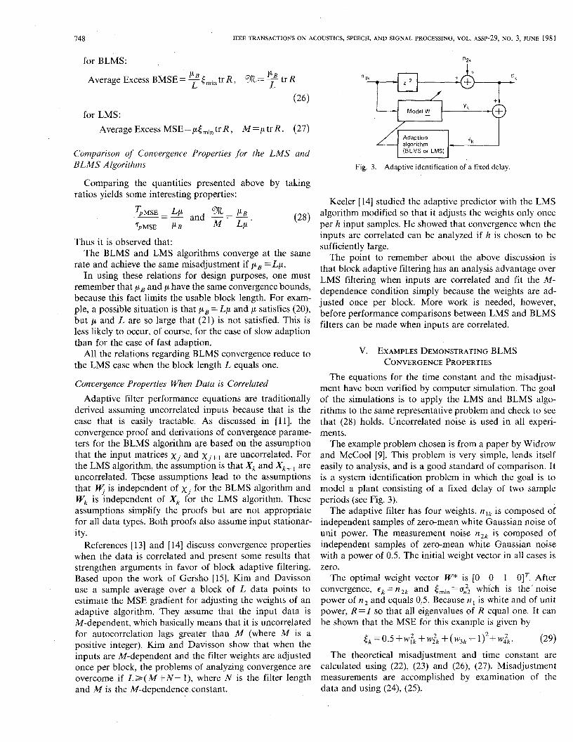
Fig. 3. Adaptive identification of a fixed delay

Keeler [ 141 studied the, adaptive predictor with the LMS algorithm modified so that it adjusts the weights only once per h input samples. He showed that convergence when the inputs are correlated can be analyzed if h is chosen to be sufficiently large.

The point to remember about the above discussion is that block adaptive filtering has an analysis advantage over LMS filtering when inputs are correlated and fit the M- dependence condition simply because the weights are adjusted once per block. More work is needed, however, before performance comparisons between LMS and BLMS filters can be made when inputs are correlated.

V. EXAMPLES DEMONSTRATING BLMS CONVERGENCE PROPERTIES

The equations for the time constant and the misadjustment have been verified by computer simulation. The goal of the simulations is to apply the LMS and BLMS algorithms to the same representative problem and check to see that (28) holds. Uncorrelated noise is used in all experiments.

The example problem chosen is from a paper by Widrow and McCool [9]. This problem is very simple, lends itself easily to analysis, and is a good standard of comparison. It is a system identification problem in which the goal is to model a plant consisting of a fixed delay of two sample periods (see Fig. 3).

The adaptive filter has four weights. nlk is composed of independent samples of zero-mean white Gaussian noise of unit power. The measurement noise n2, is composed of independent samples of zero-mean white Gaussian noise with a power of 0.5. The initial weight vector in all cases is zer 0.

The optimal weight vector W* is [0 0 1 0IT. After convergence, E , = n2, and tmin = c,i which is the “noise power of n 2 and equals 0.5. Because n , is white and of unit power, R = I so that all eigenvalues of R equal one. It can be shown that the MSE for this example is given by

The theoretical misadjustment and time constant are calculated using (22), (23) and (26), (27). Misadjustment measurements are accomplished by examination of the data and using (24), (25).

CLARK et al. : BLOCK IMPLEMENTATION OF DIGITAL FILTERS

1.6 -1 1 . 6 7

Time index k Time index k

Individual learning a w e Ensemblaaverageof32learningaNer

0'41 0.2

1W Time index k

200 3W OO l W 2w Time index k

Individual learntng curve Enmble avYeraC Of 32 learning E U N e 3

Fig. 4. (a) Experiment AI-LMS algorithm. (bj Experiment Al- BLMS algorithm.

$ ;''\ a 1.2 1.0

I E

0.8

( 4 (bj Fig. 5. Experiment A2-LMS and BLMS algorithms.

A1

10 0.234 107 110 9.375% l o $ 0.0234 10.7 1 1 9.375% 10% 01 1W 0.0234 1070 11W 0.1035% 0.1% 0.0234 10.7 1 1 9.375% 10% A2 2 0.0234 21.4 21.4 4.68% 48% 0.0234 10.7 1 1 9.375% 10%

1W 0.1 250 250 04% 0.46% 0.001 250 250 0.4% 0.4% 82

Experiment A This experiment gives examples showing that when p B =

p, TMSE= LrMSEand Em=M/L. Learning curves are shown in Figs. 4 and 5, and the results are summarized in Table I.

749

1.6 I 1 I I / 1.6 I I :I 1 .o

0.8

0.6

o ' 8 [ 0.6 L] :::I , 1 0 40 80 120 0 4ca 9 W 1200

Ensemble average of 32 learning C U N ~

Time index k

Enrembleaerageof32leamingcurwr

Time #&x k

( 4 (b) Fig. 6. Experiment B1 -LMS and BLMS algorithms.

Fig. 7. Experiment B2-LMS and BLMS algorithms.

Close agreement between theoretical and experimental results is observed.

Experiment B This experiment gives examples showing that when p =

Lp, TMSE = rMsE and Em= M . Learning curves are shown in Figs. 6 and 7, and the results are summarized in Table I. Once again, close agreement between theoretical and experimental results is observed.

Many more experiments using the above and other rela- tionships between pB, 1.1, and L have been performed and show that (28) holds.

VI. COMPUTATIONAL COMPLEXITY OF LMS AND BLMS ADAPTIVE FILTERING

The main computational efficiency issues involved in algorithm implementation are storage (memory), time (number of machine cycles for CPU, input-output, etc.), and computational complexity measured in the number of real multiplies and adds required. Because the first two issues are processor architecture-dependent, this paper con- centrates on the computational complexity required when using a standard serial-type processor. This is done for convenience, even though the most efficient implementation of BLMS adaptive filters is probably with parallel processors.

750 IEEE TRANSACTIONS ON ACOUSTICS, SPEECH, AND SIGNAL PROCESSING, VOL. ASSP-29, NO. 3, JUNE 198 1

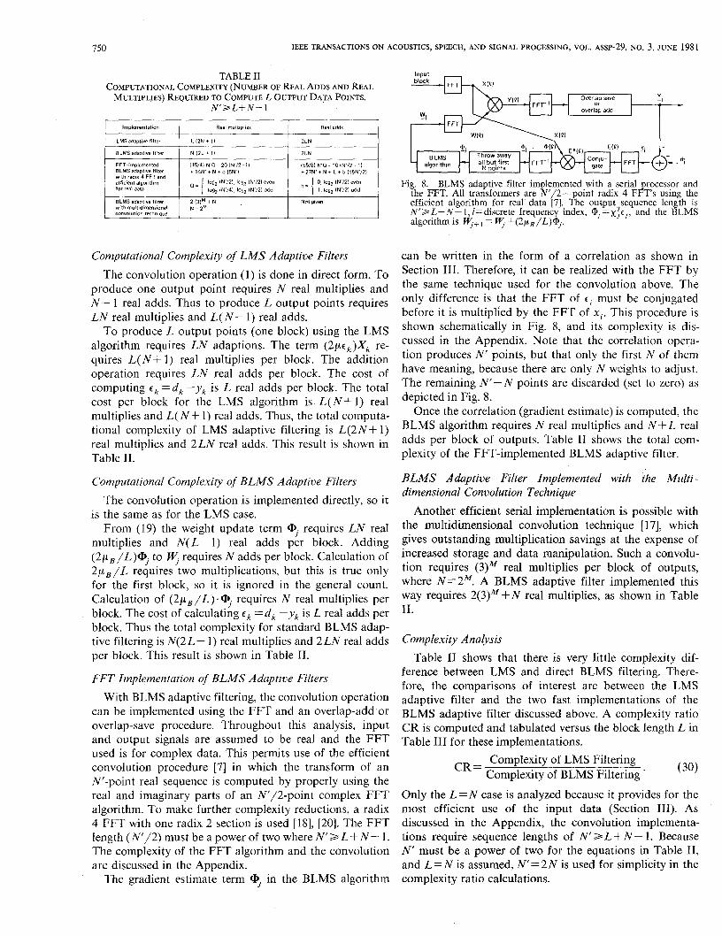
TABLE I1 COMPUTATIONAL COMPLEXITY (NUMBER OF REAL ADDS AND REAL

MULTIPLIES) REQUIRED TO COMPUTE L OUTPUT DATA POINTS. N'>L+N-I

Computational Complexity of LMS Adaptive Filters The convolution operation (1) is done in direct form. To

produce one output point requires N real multiplies and N- 1 real adds. Thus to produce L output points requires LN real multiplies and L( N- 1) real adds.

To produce L output points (one block) using the LMS algorithm requires LN adaptions. The term (2pck)Xk requires L( N+ 1) real multiplies per block. The addition operation requires LN real adds per block. The cost of computing c k =d, -y, is L real adds per block. The total cost per block for the LMS algorithm i s 'L (N+ 1) real multiplies and L( N + 1) real adds. Thus, the total computational complexity of LMS adaptive filtering is L(2N+ 1) real multiplies and 2LN real adds. This result is shown in Table 11.

Computational Complexity of BLMS Adaptive Filters The convolution operation is implemented directly, so it

is the same as for the LMS case. From (19) the weight update term aj requires LN real

multiplies and N(L- 1) real adds per block. Adding (2pB/L)aj to W , requires N adds per block. Calculation of 2 p B / L requires two multiplications, but this is true only for the first block, so it is ignored in the general count. Calculation of (2pB/L)'@, requires N real multiplies per block. The cost of calculating c k =d, - y k is L real adds per block. Thus the total complexity for standard BLMS adaptive filtering is N(2 L+ 1) real multiplies and 2 LN real adds per block. This result is shown in Table 11.

FFT Implementation of BLMS Adaptive Filters With BLMS adaptive filtering, the convolution operation

can be implemented using the FFT and an overlap-add.or overlap-save procedure. Throughout this analysis, input and output signals are assumed to be real and the FFT used is for complex data. This permits use of the efficient convolution procedure [7] in which the transform of an N'-point real sequence is computed by properly using the real and imaginary parts of an N'/2-point complex FFT algorithm. To make further complexity reductions, a radix 4 FFT with one radix 2 section is used [IS], [20]. The FFT length (N'/2) must be a power of two where N ' 3 L + N- 1. The complexity of the FFT algorithm and the convolution are discussed in the Appendix.

The gradient estimate term ai in the BLMS algorithm

block

overlap add

FFT

Fig. 8. BLMS adaptive filter implemented with a serial processor and

efficient algorithm for real. data [7]. The output sequence length is the FFT. All transformers are N'/2-point radix 4 FFT's using the

N'>Z,+.N-l,I=discrete frequency index, @, =xye,, and the BLMS algorithm is wJ+, = "; +(2pB/L)Qj.

can be written in the form of a correlation as shown in Section 111. Therefore, i t can be realized with the FFT by the same technique used for the convolution above. The only difference is that the FFT of c i must be conjugated before it is multiplied by the FFT of xi. This procedure is shown schematically in Fig. 8, and its complexity is discussed in the Appendix. Note that the correlation operation produces N' points, but that only the first N of them have meaning, because there are only N weights to adjust. The remaining N'- N points are discarded (set to zero) as depicted in Fig. 8.

Once the correlation (gradient estimate) is computed, the BLMS algorithm requires N real multiplies and N + L real adds per block of outputs. Table 11 shows the total complexity of the FFT-implemented BLMS adaptive filter.

BLMS Adaptive Filter Implemented with the Multi- dimensional Convolution Technique

Another efficient serial implementation is possible with the multidimensional convolution technique [ 171, which gives outstanding multiplication savings at the expense of increased storage and data manipulation. Such a convolution requires (3)M real multiplies per block of outputs, where N=2M. A BLMS adaptive filter implemented this way requires 2(3)M+N real multiplies, as shown in Table 11.

Complexity Analysis Table I1 shows that there is very little complexity dif-

ference between LMS and direct BLMS filtering. There- fore, the comparisons of interest are between the LMS adaptive filter and the two fast implementations of the BLMS adaptive filter discussed above. A complexity ratio CR is computed and tabulated versus the block length L in Table 111 for these implementations.

CR= Complexity of LMS Filtering Complexity of BLMS Filtering . (30)

Only the L=N case is analyzed because it provides for the most efficient use of the input data (Section 111). As discussed in the Appendix, the convolution implementations require sequence lengths of N'>L+ N- 1. Because N' must be a power of two for the equations in Table 11, and L = N is assumed, N'=2N is used for simplicity in the complexity ratio calculations.

CLARK et d.: BLOCK IMPLEMENTATION OF DIGITAL FILTERS

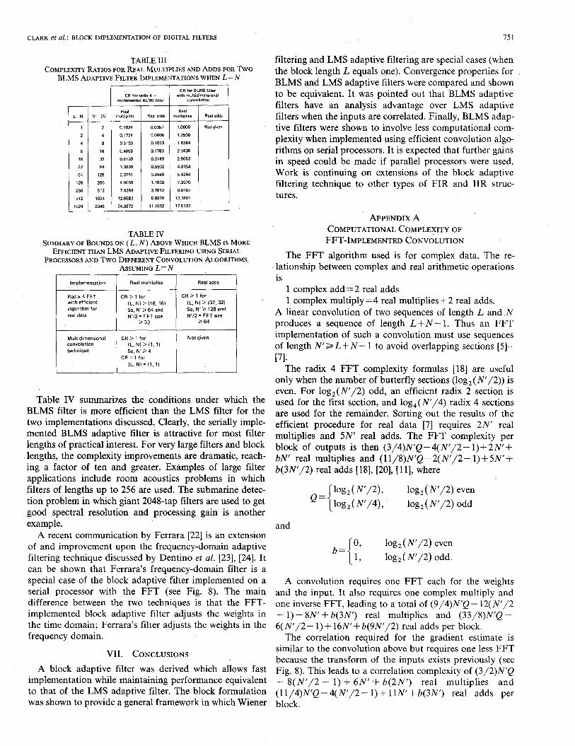
TABLE I11 COMPLEXITY RATIOS FOR REAL MULTIPLIES AND ADDS FOR T W O

BLMS ADAPTIVE FILTER IMPLEMENTATIONS WHEN L=N

- L = N -

1

2

4

8

16

32

64

128

256

512

1024 -

__ N’= 2N __

2

4

8

16

32

64

128

256

512

1024

2048 ~

Real multiplber

0.1034

0.1724

0.3103

0.4658

0.8199

2.3751

1.3098

4 . w m

7.4264

12.9683

24.3872

TABLE IV SUMMARY OF BOUNDS ON ( L , N ) ABOVE WHICH BLMS IS MORE

EFFICIENT THAN LMS ADAPTIVE FILTERING USING SERIAL PROCESSORS AND T W O DIFFERENT CONVOLUTION ALGORITHMS,

ASSUMING L= N

with efficient Radlx 4 F F T

algorithm for real data

Multldimensional convolution technique

7-

I

Real multlplles

CR > 1 for (L, N) > (16, 161 So, N’ > 64 and N’l2 = FFT size

Z 32

CR > 1 for (L. N) > (1. 1) SO, N’ > 4

CR = 1 for (L. Nl= (1, 1)

Real adds

CR 2 1 for

So. N’ 128 and IL. NI > (32. 32)

N’/2 = F F T size 2 64

Not given I

Table IV summarizes the conditions under which the BLMS filter is more efficient than the LMS filter for the two implementations discussed. Clearly, the serially implemented BLMS adaptive filter is attractive for most filter lengths of practical interest. For very large filters and block lengths, the complexity improvements are dramatic, reach- ing a factor of ten and greater. Examples of large filter applications include room acoustics problems in which filters of lengths up to 256 are used. The submarine detection problem in which giant 2048-tap filters are used to get good spectral resolution and processing gain is another example.

A recent communication by Ferrara [22] is an extension of and improvement upon the frequency-domain adaptive filtering technique discussed by Dentino et al. [23], [24]. It can be shown that Ferrara’s frequency-domain filter is a special case of the block adaptive filter implemented on a serial processor with the FFT (see Fig. 8). The main difference between the two techniques is that the FFT- implemented block adaptive filter adjusts the weights in the time domain; Ferrara’s filter adjusts the weights in the frequency domain.

VII. CONCLUSIONS A block adaptive filter was derived which allows fast

implementation while maintaining performance equivalent to that of the LMS adaptive filter. The block formulation was shown to provide a general framework in which Wiener

75 1

filtering and LMS adaptive filtering are special cases (when the block length L equals one). Convergence properties for BLMS and LMS adaptive filters were compared and shown to be equivalent. It was pointed out that BLMS adaptive filters have an analysis advantage over EMS adaptive filters when the inputs are correlated. Finally, BLMS adaptive filters were shown to involve less computational complexity when implemented using efficient convolution algorithms on serial processors. It is expected that further gains in speed could be made if parallel processors were used. Work is continuing on extensions of the block adaptive filtering technique to other types of FIR and IIR structures.

APPENDIX A COMPUTATIONAL COMPLEXITY OF FFT-IMPLEMENTED CONVOLUTION

The FFT algorithm used is for complex data. The re- lationship between complex and real arithmetic operations is

1 complex add=2 real adds 1 complex multiply=4 real multiplies+2 real adds.

A linear convolution of two sequences of length L and N produces a sequence of length L S N - 1. Thus an FFT implementation of such a convolution must use sequences of length N‘ > L+ N - 1 to avoid overlapping sections [5]-

The radix 4 FFT complexity formulas [ 181 are useful only when the number of butterfly sections (log,( N’/2)) is even. For log,( N ’ / 2 ) odd, an efficient radix 2 section is used for the first section, and log, (N’/4) radix 4 sections are used for the remainder. Sorting out the results of the efficient procedure for real data [7] requires 2 N real multiplies and 5N’ real adds. The FFT complexity per block of outputs is then (3/4)N’Q-4(N’/2- 1)+ 2 N + bN’ real multiplies and (1 1/8)N’Q - 2( N’/2 - 1) + 5N’ + b(3N‘/2) real adds [18], [20], [ l l] , where

~71.

Q={ log, ( N’/2), log, (N’/2) even log, ( N’/4), log, ( N’/2) odd

and

h={ 0 , log,( ~ ’ / 2 ) even 1, log, (N’/2) odd.

A convolution requires one FFT each for the weights and the input. It also requires one complex multiply and one inverse FFT, leading to a total of (9/4)N’Q- 12(N’/2 - 1) + 8N‘ + b(3N’) real multiplies and (33/8)N’Q - 6( N’/2- 1)+ 16N’+b(9N’/2) real adds per block.

The correlation required for the gradient estimate is similar to the convolution above but requires one less FFT because the transform of the inputs exists previously (see Fig. 8). This leads to a correlation complexity of (3/2)N’Q - 8(N’/2 - 1) + 6N’ + b(2N’) real multiplies and (1 1/4)N’Q - 4( N’/2 - 1) + 11N’ + b(3N’) real adds per block.


ACKNOWLEDGMENT The authors gratefully acknowledge Dr. R. Twogood for

his many helpful suggestions.

[91

1121

u31

1231

~ 4 1

REFERENCES C. Burrus, “Block implementation of digtal filters,” IEEE Trans. Circuit Theory, vol. CT-18, Nov. 1971. -, “Block realization of digital filters,” IEEE Trans. Audio Electroacoust., vol. AU-20, Oct. 1972.

sive digital filters-New structures and properties,” IEEE Trans. S. K. Mitra and R. Gnanasekaran, “Block implementation of recur-

Circuit Theory, vol. CAS-25, Apr. 1978. R. Gnanasekaran and S. K. Mitra, “A note on block implementa-

A. V. Oppenheim and R. W. Schafer, Digital Signal Processing. tion of IIR digital filters,” Proc. IEEE, vol. 65, July 1977.

New Jersey: Prentice-Hall, 1975. L. R. Rabiner and B. Gold, Theov and Application of Digital Signal

E. 0. Brigham, The Fast Fourier Transform. New Jersey: Prentice- Processing. New Jersey: Prentice-Hall, 1975.

Hall, 1974. B. Widrow, J. McCool, M. Larimore, and C. Johnson, “Stationary and nonstationary learning characteristics of the LMS adaptive filter,” Proc. IEEE, vol. 64, August 1976. B. Widrow, and J. M. McCool, “A Comparison of Adaptive Algo- rithms Based on the Methods of Steepest Descent and Random Search,” IEEE Trans. Antennas and Propagation. Vol. AP-24. No. 5. September 1976. B. Widrow, P. E. Mantey, L. J. Griffiths, and B. B. Goode, “Adaptive antenna systems,” Proc. IEEE, vol. 55, Dec. 1967.

event detection,” Ph.D. dissertation, Univ. of California, Santa 6. A. Clark, “Block adaptive filtering and its Application to Seismic

Barbara (in preparation), 1981. H. C. Andrews, and B. R. Hunt, Digital Image Restoration. New Jersev: Prentice-Hall. 1977. J. K.‘ Kim and L. D , Davisson, “Adaptive linear estimation for stationary M-dependent processes,” IEEE Trans. Inform. Theory, vol. IT-21, Jan. 1975. R. J. Keeler, “Non-optimal convergence of adaptive LMS with uncorrelated data.” in IEEE Int. Conf. Acoustics. Sueech. Sianal Processing, 1978. A. Gersho, “Convergence properties of an adaptive filtering algorithm,” in Proc. 1968 Asilomar Conf. on Circuits and Systems, (Pacific Grove, CA), pp. 302-304. A. Gersho, “Adaptive equalization of highly dispersive channels for data transmission,” Bell Syst. Tech. J . , pp. 55-70, Jan. 1969.

convolution by multidimensional techniques,” IEEE Trans. Acous- R. C. Aganval and C. S. Burrus, “Fast one-dimensional digital

tics, Speech, Signal Processing, vol. ASSP-22, pp. 1 - 10, Feb. 1974. R. C. Singleton, “An Algorithm for computing the mixed radix fast

pp. 93- 103, June 1969. Fourier transform,” IEEE Trans. Audio E/ectroacoust., vol. AU-17,

J. Treichler, private communication. R. E. Twogood, private communication. G. A. Clark, S. K. Mitra, and S. R. Parker, “Block adaptive filtering,” in 1980 IEEE Int. Symp. on Circuits and Systems, (Hous- ton, TX), Apr. 1980, pp. 384-387. E. R. Ferrara, “Fast implementation of LMS adaptive filters,”

Aug. 1980. IEEE Trans. Acoustics, Speech, Signal Processing, vol. ASSP-28,

M. J. Dentino, J. McCool, and B. Widrow, “Adaptive filtering in the frequency domain,” Proc. IEEE, vol. 66, Dec. 1968. T. Waltzman and M. Schwartz, “Automatic equalization using the discrete frequency domain,” IEEE Trans. Inform. Theory, vol. IT-19, Jan. 1973. B. Widrow, “Adaptive filters,” in Aspects of Network and System

Rinehart. and Winston. Inc.. 1970. Theory, (ed. R. E. Kalman and N. Declaris), New York: Holt,

, 1 , -

B: Widrow, et al., “Adaptive noise cancelling: Principles and applications,” Proc. IEEE, vol. 63, Dec. 1975.

Gregory A. Clark (S’69-M72-S’77) was born in Lafayette, IN, on April 17, 1950. He completed the electrical engineering Honors Program at Purdue University, ’M’est Lafayette, IN, receiving the B.S.E.E. and M.S.E.E. degrees in 1972 and 1974, respectively. In 1977, he began a Ph.D. program at the University of California, Santa Barbara, where he is currently a doctoral candi- date.

He was a graduate teaching assistant at Purdue from 1972- 74, atld was employed by the Mariner

Telecommunications Group of the Caltech Jet Propulsion Laboratory, Pasadena, CA, during the summer of 1973. Since 1974, he has been with the University of California Lawrence Livermore National Laboratory, where he works in the Engineering Research Division. At LLNL, he has been concerned with computerized chemistry instrumentation, modeling of material control instruments, image processing, adaptive filtering, large-scale estimation, and seismic event detection. His research interests are in the theory and application of control, estimation/detection, and digital signal processing.

Mr. Clark is a member of Eta Kappa Nu.

Sanjit K. Mitra (S’59-M63-SM69-F774) received the M.S. and Ph.D. degrees in electrical engineering from the University of California, Berkeley, in 1960 and 1962, respectively.

He has been on the faculty at the University of California since 1967, first at the Davis campus and more recently at the Santa Barbara campus as a Professor of Electrical and Computer En- gineering. In July of 1979 he was appointed Chairman of the Department of Electrical and Computer Engineering, College of Engineering,

at UCSB. He is a Consultant to the Lawrence Livermore Laboratory, University of California, Livermore, and a Consulting Editor for the Electricul/Computer Science and Engineering Series of Van Nostrand Reinhold Company, New York. He has published a number of papers in active and passive networks and digital filters, and is the author of Analysis and Synthesis of Lineur Active Networks and An Introduction to Digital and Analog Integruted Circuits and Applications, and Editor of Active Inductorless Filters, Co-editor of Modern Filter Theory and Design (with G. C. Temes), and Co-editor of Two-Dimensional Digital Signul Processing (with M. P. Ekstrom). He holds two patents in active filters.

Dr. Mitra is a member of the American Society for Engineering Education, Sigma Xi and Eta Kappa Nu. He was an Associate Editor of the IEEE TRANSACTIONS ON Circuit Theory, a member of the Administra- tive Committee of the IEEE Circuits and Systems Society, General Chairman of the 1974 IEEE International Symposium on Circuits and Systems, a member of the editorial board of the IEEE Press, and is presently a member of the editorial board of the PROCEEDINGS OF THE IEEE. He is the recipient of the 1973 F. E. Terman Award of the American Society of Engineering Education.

Sydney R. Parker (S’43-M45-SM51-F’75), for a photograph and biog- raphy please see page 466 of this issue.

Block implementation of adaptive digital filters

Documents

Transcript of Block implementation of adaptive digital filters