Speed sensorless control of a DC-motor via adaptive filters
10
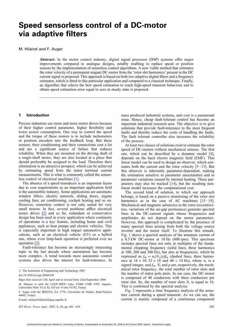
Speed sensorless control of a DC-motor via adaptive filters M. Hilairet and F. Auger Abstract: In the motor control industry, digital signal processor (DSP) systems offer major improvements compared to analogue designs, notably enabling to replace speed or position sensors by the implementation of sensorless control algorithms. A new viable method that estimates the rotor velocity of a permanent magnet DC-motor from the ‘rotor slot harmonics’ present in the DC current signal is proposed. This approach is based on both two adaptive digital filters and a frequency estimator, which is fitted to this particular application and compared to a classical technique. Finally, an algorithm that selects the best speed estimation to reach high-speed transient behaviour and to obtain speed estimation error equal to zero at steady state is proposed. 1 Introduction Process industries use more and more motor drives because of their higher control parameter, higher flexibility and lower power consumption. One way to control the speed and the torque of these motors is to include tachometers or position encoders into the feedback loop. But these sensors, their conditioning and their connections cost a lot and are a significant source of failure that reduces reliability. When they are mounted on the driving shaft of a single-shaft motor, they are also located at a place that should preferably be assigned to the load. Therefore their elimination is an attractive prospect, which can be achieved by estimating speed from the stator terminal current measurements. This is what is commonly called the sensor- less control of electrical machines [1]. The absence of a speed transducer is an important factor due to cost requirements as an important application field is the automobile industry. Some applications are automatic window lifters, electric sunroofs, sliding doors, engine cooling fans, air conditioning, cockpit heating and so on. However, sensorless control is not only suited for very small motors. In fact, several problems afflict electrical motor drives [2] and so far, redundant or conservative design has been used in every application where continuity of operations is a key feature, including home and civil appliances, such as heat pumps and electric vehicles. This is especially important in high impact automotive appli- cations, such as an electrical vehicle (EV) or a hybrid one, where even limp-back operation is preferred over no operation [3]. Fault-tolerance has become an increasingly interesting topic in the last decade where automation has become more complex. A trend towards more autonomic control systems also drives the interest for fault-tolerance. In mass produced industrial systems, unit cost is a paramount issue. Hence, cheap fault-tolerant control has become an important industrial research area. The objective is to give solutions that provide fault-tolerance to the most frequent faults and thereby reduce the costs of handling the faults. The fault tolerant controller also increases the reliability of the process. At least two classes of solutions exist to estimate the rotor speed of DC-motors without mechanical sensors. The first one, which can be described by a dynamic model [4], depends on the back electro magnetic field (EMF). This linear model can be used to design an observer, which esti- mates both the current and the rotor velocity [5–13]. But this observer is inherently parameter-dependent, making the estimation sensitive to parameter uncertainties and to parameter variations caused by internal heating. These par- ameters may also be tracked [14], but the resulting non- linear model increases the computational cost. The second kind of solution, to which our approach belongs, is based on a passive monitoring of the rotor slot harmonics as in the case of AC machines [15–19]. Mechanical and magnetic saliencies in the rotor (eccentrici- ties, variations of the air-gap permeance) generate spectral lines in the DC-current signals whose frequencies and amplitudes do not depend on the motor parameters. However, this approach is complicated by the presence of many spectral lines arising from both the voltage source inverter and the motor itself. To illustrate this remark, Fig. 1 shows a spectral analysis of the armature current of a 0.5 kW DC-motor at 10 Hz (600 rpm). This spectrum includes spectral lines not only at multiples of the funda- mental chopping frequency (solid lines, three harmonics at 100, 200 and 300 Hz), but also at frequencies, which be expressed as f sh ¼ n r ðN r =pÞf m (dashed lines, three harmo- nics at 16 10; 32 10 and 48 10 Hz), where n r is a signed integer, and f m ; N r and p are, respectively, the mech- anical rotor frequency, the total number of rotor slots and the number of stator pole pairs. In our case, the DC-motor is composed of 48 conductors with three conductors per rotor slot. So, the number of rotor slots N r is equal to 16. This is confirmed by the spectral analysis. Fig. 2 represents a time frequency analysis of the arma- ture current during a speed transient. As we can see, the current is mainly composed of a continuous component # The Institution of Engineering and Technology 2007 doi:10.1049/iet-epa:20060149 Paper first received 13th April and in revised form 22nd September 2006 M. Hilairet is with the LGEP/SPEE Labs, CNRS UMR 8705, Supelec, Universites Paris VI et XI, Gif sur Yvette 91192, France F. Auger with the IREENA, EA 1770, Universites de Nantes, Saint-Nazaire 44602, France E-mail: [email protected] IET Electr. Power Appl., 2007, 1, (4), pp. 601–610 601 Authorized licensed use limited to: University of Nantes. Downloaded on November 26, 2009 at 04:23 from IEEE Xplore. Restrictions apply.
-
Upload
independent -
Category
Documents
-
view
0 -
download
0
Transcript of Speed sensorless control of a DC-motor via adaptive filters
Speed sensorless control of a DC-motorvia adaptive filters
M. Hilairet and F. Auger
Abstract: In the motor control industry, digital signal processor (DSP) systems offer majorimprovements compared to analogue designs, notably enabling to replace speed or positionsensors by the implementation of sensorless control algorithms. A new viable method that estimatesthe rotor velocity of a permanent magnet DC-motor from the ‘rotor slot harmonics’ present in the DCcurrent signal is proposed. This approach is based on both two adaptive digital filters and a frequencyestimator, which is fitted to this particular application and compared to a classical technique. Finally,an algorithm that selects the best speed estimation to reach high-speed transient behaviour and toobtain speed estimation error equal to zero at steady state is proposed.
1 Introduction
Process industries use more and more motor drives becauseof their higher control parameter, higher flexibility andlower power consumption. One way to control the speedand the torque of these motors is to include tachometersor position encoders into the feedback loop. But thesesensors, their conditioning and their connections cost a lotand are a significant source of failure that reducesreliability. When they are mounted on the driving shaft ofa single-shaft motor, they are also located at a place thatshould preferably be assigned to the load. Therefore theirelimination is an attractive prospect, which can be achievedby estimating speed from the stator terminal currentmeasurements. This is what is commonly called the sensor-less control of electrical machines [1].
The absence of a speed transducer is an important factordue to cost requirements as an important application fieldis the automobile industry. Some applications are automaticwindow lifters, electric sunroofs, sliding doors, enginecooling fans, air conditioning, cockpit heating and so on.However, sensorless control is not only suited for verysmall motors. In fact, several problems afflict electricalmotor drives [2] and so far, redundant or conservativedesign has been used in every application where continuityof operations is a key feature, including home and civilappliances, such as heat pumps and electric vehicles. Thisis especially important in high impact automotive appli-cations, such as an electrical vehicle (EV) or a hybridone, where even limp-back operation is preferred over nooperation [3].
Fault-tolerance has become an increasingly interestingtopic in the last decade where automation has becomemore complex. A trend towards more autonomic controlsystems also drives the interest for fault-tolerance. In
# The Institution of Engineering and Technology 2007
doi:10.1049/iet-epa:20060149
Paper first received 13th April and in revised form 22nd September 2006
M. Hilairet is with the LGEP/SPEE Labs, CNRS UMR 8705, Supelec,Universites Paris VI et XI, Gif sur Yvette 91192, France
F. Auger with the IREENA, EA 1770, Universites de Nantes, Saint-Nazaire44602, France
E-mail: [email protected]
IET Electr. Power Appl., 2007, 1, (4), pp. 601–610
Authorized licensed use limited to: University of Nantes. Downloaded on November 26, 20
mass produced industrial systems, unit cost is a paramountissue. Hence, cheap fault-tolerant control has become animportant industrial research area. The objective is to givesolutions that provide fault-tolerance to the most frequentfaults and thereby reduce the costs of handling the faults.The fault tolerant controller also increases the reliabilityof the process.
At least two classes of solutions exist to estimate the rotorspeed of DC-motors without mechanical sensors. The firstone, which can be described by a dynamic model [4],depends on the back electro magnetic field (EMF). Thislinear model can be used to design an observer, which esti-mates both the current and the rotor velocity [5–13]. Butthis observer is inherently parameter-dependent, makingthe estimation sensitive to parameter uncertainties and toparameter variations caused by internal heating. These par-ameters may also be tracked [14], but the resulting non-linear model increases the computational cost.
The second kind of solution, to which our approachbelongs, is based on a passive monitoring of the rotor slotharmonics as in the case of AC machines [15–19].Mechanical and magnetic saliencies in the rotor (eccentrici-ties, variations of the air-gap permeance) generate spectrallines in the DC-current signals whose frequencies andamplitudes do not depend on the motor parameters.However, this approach is complicated by the presence ofmany spectral lines arising from both the voltage sourceinverter and the motor itself. To illustrate this remark,Fig. 1 shows a spectral analysis of the armature current ofa 0.5 kW DC-motor at 10 Hz (600 rpm). This spectrumincludes spectral lines not only at multiples of the funda-mental chopping frequency (solid lines, three harmonicsat 100, 200 and 300 Hz), but also at frequencies, which beexpressed as fsh ¼ nrðNr=pÞfm (dashed lines, three harmo-nics at 16 � 10; 32 � 10 and 48 � 10 Hz), where nr is asigned integer, and fm;Nr and p are, respectively, the mech-anical rotor frequency, the total number of rotor slots andthe number of stator pole pairs. In our case, the DC-motoris composed of 48 conductors with three conductors perrotor slot. So, the number of rotor slots Nr is equal to 16.This is confirmed by the spectral analysis.
Fig. 2 represents a time frequency analysis of the arma-ture current during a speed transient. As we can see, thecurrent is mainly composed of a continuous component
601
09 at 04:23 from IEEE Xplore. Restrictions apply.
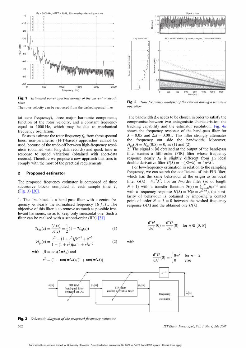
(at zero frequency), three major harmonic components,function of the rotor velocity, and a constant frequencyequal to 1000 Hz, which may be due to mechanicalfrequency oscillation.
So as to estimate the rotor frequency fm from these spectrallines, non-parametric (FFT-based) approaches cannot beused, because of the trade-off between high-frequency resol-ution (obtained with long-data records) and quick time inresponse to speed variations (obtained with short-datarecords). Therefore we propose a new approach that tries tocomply with the most of the practical requirements.
2 Proposed estimator
The proposed frequency estimator is composed of threesuccessive blocks computed at each sample time Ts
(Fig. 3) [20].
1. The first block is a band-pass filter with a centre fre-quency l0 nearly the normalised frequency 16 fmTs. Theobjective of this filter is to remove as much as possible irre-levant harmonic, so as to keep only sinusoidal one. Such afilter can be realised with a second-order (IIR) [21]
HpbðzÞ ¼Y1ðzÞ
XðzÞ¼
1
2ð1 �HptðzÞÞ ð1Þ
HptðzÞ ¼r2
� ð1 þ r2Þbz�1
þ z�2
1 � ð1 þ r2Þbz�1 þ r2z�2ð2Þ
with b ¼ cosð2pl0Þ and
r2¼ ð1 � tanðpDlÞ=ð1 þ tanðpDlÞÞ
0 500 1000 1500 2000 2500−90
−80
−70
−60
−50
−40
−30
−20
−10
0
frequency (Hz)
PS
D (
dB)
Fs = 5000 Hz, NFFT = 2048, 80% overlap, Hamming window
Fig. 1 Estimated power spectral density of the current in steadystate
The rotor velocity can be recovered from the dashed spectral lines
602
Authorized licensed use limited to: University of Nantes. Downloaded on November 26, 2
The bandwidth Dl needs to be chosen in order to satisfy thecompromise between two antagonistic characteristics: thetracking capability and the estimator resolution. Fig. 4ashows the frequency response of the band-pass filter forl ¼ 0:05 and Dl ¼ 0:001. This filter strongly attenuatesthe frequency out side the bandwidth. Moreover,Hpbð0Þ ¼ Hpbð0:5Þ ¼ 0, as (1) and (2).2. The signal y1½n� obtained at the output of the band-passfilter excites a fifth-order (FIR) filter whose frequencyresponse nearly l0 is slightly different from an idealdouble derivative filter GðlÞ ¼ �ð |2plÞ2 ¼ 4p2l2.
For low-frequency estimation in relation to the samplingfrequency, we can search the coefficients of this FIR filter,which has the same behaviour at the origin as an ideal
filter GðlÞ ¼ 4p2l2. For an N-order filter (so of length
N þ 1) with a transfer function HðzÞ ¼PN
k¼0hkz�k and
with a frequency response HðlÞ ¼ Hðz ¼ e|2plÞ, the simi-larity of behaviour is obtained by imposing a contactpoint of order N at l ¼ 0 between the wished frequencyresponse GðlÞ and the obtained one HðlÞ
dnH
dlnð0Þ ¼
dnG
dlnð0Þ for n [ ½0;N �
with
dnG
dlnð0Þ ¼
8p2 for n ¼ 2
0 else
�
−0.02
0
0.02
0.04
0.06
Rea
l par
t
Signal in time
Log. scale [dB]
Ene
rgy
spec
tral
den
sity
SP, Lh=100, Nf=128, log. scale, imagesc, Threshold=0.001%
Time [ms]
Fre
quen
cy [k
Hz]
0 200 400 600 800 1000 1200 14000
0.5
1
1.5
2
Fig. 2 Time frequency analysis of the current during a transientoperation
Fig. 3 Schematic diagram of the proposed frequency estimator
IET Electr. Power Appl., Vol. 1, No. 4, July 2007
009 at 04:23 from IEEE Xplore. Restrictions apply.

Fig. 4 Frequency response of the band-pass filter and double derivative filter
a Band-pass filter with l ¼ 0.05 and Dl ¼ 0.001b Double derivative filter with l ¼ 0 (i), l ¼ 0.25 (ii), and l ¼ 0.175 (iii)
These relations lead to a linear system of dimension N þ 1,which is
XNk¼0
knhk ¼�2 for n ¼ 2
0 else
�
The coefficients hk are the solution of a Vandermodesystem. For N ¼ 5, the solution is
h0 ¼ �45
12h1 ¼
154
12h2 ¼ �
214
12
h3 ¼156
12h4 ¼ �
61
12h5 ¼
10
12
The frequency response is close to that of an ideal doublederivative filter (Fig. 4b (i)) for jlj , 0:12, so forFs . 10 f . The use of higher-order filters does not seemto be justified because their behaviours are not significantlybetter. On the other hand, for jlj . 0:12, it is necessary touse an adjustable filter parametrised by the normalised fre-quency l where its behaviour at l is near an ideal doublederivative filter. For a fifth order FIR filter, the transferfunction and frequency response are
HðzÞ ¼ h0 þ h1z�1
þ � � � þ h5z�5
HðlÞ ¼ h0 þ h1e�|2pl
þ � � � þ h5e�|10pl
This principle leads to impose the followings relations asfollows
Hðl0Þ ¼ Hð�l0Þ ¼ Gðl0Þ ¼ 4p2l20
H0ðl0Þ ¼ �H
0ð�l0Þ ¼ G
0ðl0Þ ¼ 8p2l0
H00ðl0Þ ¼ H
00ð�l0Þ ¼ G
00ðl0Þ ¼ 8p2
which form a linear system of dimension 6. With u ¼ 2pl0,the solution is
h5 ¼ð1 þ sinðuÞ2Þu� sinðuÞ cosðuÞ
2 sinðuÞ3
h4 ¼ �uþ sinðuÞð11 � 12 sinðuÞ2Þh5
2 sinðuÞ cosðuÞ
IET Electr. Power Appl., Vol. 1, No. 4, July 2007
Authorized licensed use limited to: University of Nantes. Downloaded on November 26, 20
h3 ¼u
sinðuÞ� 4 cosðuÞh4 � 2ð5 � 6 sinðuÞ2Þh5
h2 ¼ �4 cosðuÞh3 � ð10 � 12 sinðuÞ2Þh4
� 4 cosðuÞð5 � 8 sinðuÞ2Þh5
h1 ¼ �2 cosðuÞh2 � ð3 � 4 sinðuÞ2Þh3
� 4 cosðuÞð1 � 2 sinðuÞ2Þh4
� ð5 � 20 sinðuÞ2 þ 16 sinðuÞ4Þh5
h0 ¼ u2� cosðuÞh1 � cosð2uÞh2 � cosð3uÞh3
� cosð4uÞh4 � cosð5uÞh5
Figs. 4b (ii) and (iii) show the frequency response forl ¼ 0:25 and 0.175, respectively. The principal operationsfor the coefficient computation is the evaluation of
b ¼ cosðuÞ; g ¼ sinðuÞ; g2;g3; g4, and three divisions. Noother more trigonometric computation is necessarybecause of the following relations
cosð2uÞ ¼ 1 � 2 sinðuÞ2
cosð3uÞ ¼ cosðuÞð1 � 4 sinðuÞ2Þ
cosð4uÞ ¼ 1 � 8 sinðuÞ2 þ 8 sinðuÞ4
cosð5uÞ ¼ cosðuÞð1 � 12 sinðuÞ2 þ 16 sinðuÞ4Þ
3. If y1½n� ¼ A cosð2plnþ wÞ, the signal obtained at theoutput of the double derivative filter is y2½n� ¼ 4p2l2y1½n�.Because the two signals y1½n� and y2½n� are colinear, the esti-mation of l could be considered by the operation
l½n� ¼1
2p
ffiffiffiffiffiffiffiffiffiffiy2½n�
y1½n�
s¼
1
2p
ffiffiffiffiffiffiffiffiffiffiffiffiffiffiffiffiffiffiffiy1½n� y2½n�
y1½n�2
s
To avoid division by zero, the frequency is calculated by
l½n� ¼1
2p
ffiffiffiffiffiffiffiffiffiffiffiffiffiffiffiffiffiffiffiffiffiffiffiffiffiffiffiffiffiffiffiffiffiffiffiffiffiffiffiffiffiffiffiffiffiffiffiffiffiffiffiffiffiPþ1k¼0 a
ky1½n� k� y2½n� k�Pþ1k¼0 a
ky1½n� k�2
s
603
09 at 04:23 from IEEE Xplore. Restrictions apply.
with 0 � a � 1, this corresponds to the minimisationof the quadratic criterior J ðl½n�Þ ¼
Pþ1k¼0 a
kðy2½n�k�
�4p2l½n�2y1½n�k�Þ2. Obviously, this expression is computed
in a recursive form
l½n� ¼1
2p
ffiffiffiffiffiffiffiffiffiN ½n�
D½n�
s
with N ½n� ¼ aN ½n� 1� þ y1½n� y2½n�
D½n� ¼ aD½n� 1� þ y1½n�2
The parameter a has to satisfy the compromise between hightracking capabilities for fast frequency variations and theminimisation of the variance of the frequency estimationerror. Experimental results give satisfactory behaviourwith a ¼ e�2pDl [20].
Finally, to track time-varying frequencies, the frequencyl, estimated by the frequency estimator, is used at the nexttime sample to update the two filter coefficients.
3 Conventional speed estimator
A conventional method for speed estimation is the compu-tation of the discrete time state space model of the system inreal-time [5, 6, 8, 9, 11, 12]. The continuous state spacemodel of a permanent magnet DC-motor, with state spaceX ¼ ½iv�T is
dX
dt¼
�R=L �K=LK=J �f =J
� �X þ
1=L0
� �U þ
0
�1=J
� �Cr
where i;v; u and Cr are, respectively, the armature current,the rotor velocity, the armature voltage and load torque.
One solution for speed estimation is to assume the rotorvelocity nearly constant between two sample times. In thiscase the speed estimator has a low cost but it is possibleto obtain instability phenomenon in the closed-loop. Toavoid this problem, we opt for the estimation of the loadtorque. The new state space is X ¼ ½i v Cr�
T¼
½x1 x2 x3�T with transistion matrix Ac, command matrix
Bc and measurement matrix C
Ac ¼
�R=L �K=L 0
K=J �f =J 1=J
0 0 0
264
375
Bc ¼
1=L
0
0
264
375 C ¼ 1 0 0
� �
Among all the estimation techniques (Luenberger observer,Kalman filter, adaptive observer) [5, 8, 9, 11–13], wechoose the suboptimal Kalman filter (SKF) [22, 23]because of two main reasons.
† Reduced computational time, because the system islinear and stationnary. The Kalman gains are constant.† The tuning easiness of the different degrees of freedom.
A second-order series expansion of the exponentialmatrix eAcTs is sufficient for discretising the continuousstate space model with a sampling period Ts equal to
604
Authorized licensed use limited to: University of Nantes. Downloaded on November 26, 2
200ms. This leads to
Ad ¼
a11 a12 a13
a21 a22 a23
a31 a32 a33
24
35 Bd ¼
b1
b2
b3
24
35
with
a11 ¼ 1 � RTe=Lþ ðR2=L2� K2=ðLJ ÞÞT 2
e =2
a12 ¼ �KTe=Lþ ðRK=L2þ Kf =ðLJ ÞÞT2
e =2
a13 ¼ KT2e =ð2LJ Þ
a21 ¼ KTe=J � ðRK=ðLJ Þ þ fK=J ÞT 2e =2
a22 ¼ 1 � f Te=J þ ð f 2=J2� K2=ðLJ ÞÞT 2
e =2
a23 ¼ Te=J þ f T 2e =ð2J
2Þ
a31 ¼ a32 ¼ 0
a33 ¼ 1
b1 ¼ 1=L� RTe=ð2L2Þ
b2 ¼ KTe=ð2LJ Þ
b3 ¼ 0
Finally, the SKF is
x1p½k� ¼ a11x1½k � 1� þ a12x2½k � 1�
þ a13x3½k � 1� þ b1U ½k � 1�
x2p½k� ¼ a21x1½k � 1� þ a22x2½k � 1�
þ a23x3½k � 1� þ b2U ½k � 1�
e½k� ¼ y½k� � x1p½k�
x1½k� ¼ x1p½k� þ k1e½k�
x2½k� ¼ x2p½k� þ k2e½k�
x3½k� ¼ x3½k� þ k3e½k�
The three gains k1; k2 and k3 are the final values of the gainK defined by
Pp½k� ¼ AdP½k � 1�Atd þ Q
K½k� ¼ Pp½k�CtðCPp½k�C
tþ RÞ�1
P½k� ¼ Pp½k� � K½k�CPp½k�
limk!þ1K ½k� ¼
k1
k2
k3
0B@
1CA
with
R ¼ sicQ ¼
si 0 0
0 sv 0
0 0 sCr
24
35
Because R is a scalar, only the ratio Q/R is important. So,we assign to R the value 1 and we adjust the dynamics ofthe filter via the three degrees of freedom noted ða1;a2;a3Þ
R ¼ 1 Q ¼
a1 0 0
0 a2 0
0 0 a3
24
35
The degrees of freedom are adjusted so that the instan-taneous current and speed estimation are similar to the real
IET Electr. Power Appl., Vol. 1, No. 4, July 2007
009 at 04:23 from IEEE Xplore. Restrictions apply.

measure values. After trial and error loops, the selection is
a1 ¼ 10; a2 ¼ 100; a3 ¼ 0:01
4 Experimental results
An experimental validation of the proposed algorithm wascarried out on a 0.5 kW permanent magnet DC-motor,whose shaft is coupled to an induction machine (Table 1).The motor is fed by a transistor bridge chopper operatingin differential mode (þU, 2U), which received thecontrol signals from two IP regulators in cascade. This con-troller is composed of a integral action in relation to theerror, a proportional action relatively to the measuredsignal and an anti-windup action. The goal of the anti-windup action is to counteract the integration of the control-ler that produces oscillations when the control signalsaturates. This can be performed by feeding back theoutput of the saturation to the controller. Figs. 5 and 6shows the approach used for the anti-windup action.
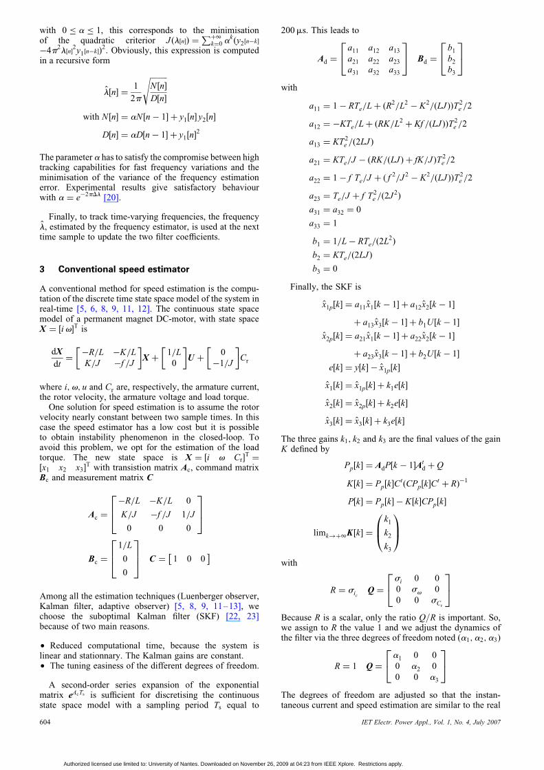
For information, the execution time of the measurement,estimation and control is given in Table 2. All the algor-ithms are developed with the C language and implementedin a TMS320C31 Digital Signal Processor of TexasInstruments with a clock frequency of 40 MHz (Fig. 7).The execution time of the frequency estimator is nearlyequal to the time required by the controller (current andspeed control). The proposed algorithm has a medium com-plexity and offers some advantages compared to state obser-vers. In fact, this speed estimator is not parameter dependentand so gives zero speed estimation error at steady state.
Fig. 8 shows a speed estimation for an operating pointat 15 Hz (900 rpm) for two different bandwidths of theIIR filter. In both cases, the average speed estimationerror is nearly equal to zero, and the variance depends onthe parameter Dl. For Dl ¼ 0:001, the speed estimationis nearly equal to the estimation value obtained from a
Table 1: Model parameters
Rated output power Pn ¼ 0.5 kW
Rated torque Cn ¼ 1.75 Nm
Rated speed N ¼ 3000 rpm
Rated voltage Vn ¼ 180 V
Rated current In ¼ 3.50 A
Resistance R ¼ 6.72 V
Inductance L ¼ 357 mH
Torque constant K ¼ 0.59 Nm/A
Inertia load J ¼ 5.4 � 1023 kgm2
Viscous coefficient f ¼ 1.6 � 1023 Nm/rad/s
Number of pole pairs p ¼ 1
Fig. 5 Speed controller with anti-windup action
IET Electr. Power Appl., Vol. 1, No. 4, July 2007
Authorized licensed use limited to: University of Nantes. Downloaded on November 26, 200
classical speed estimation algorithm [24, 25] such as
v½n� ¼um½n� � um½n� 12�
12Ts
Fig. 9 shows a speed estimation with a speed initialisation at180 rpm (þ20%) below the real value. Good estimation isreached approximately after 0.3 and 0.2 s, respectively.
Fig. 10 represents the output signals of the band-passfilter and double derivative filter, respectively, for arotational speed of 600 rpm. The harmonic at 16 times therotational frequency of the machine has an amplitude of�15 mA. The FIR filter tends to increase the noise of theoutput signal and thus deteriorates the quality of thefrequency estimation (speed).
Fig. 11 shows a linear speed variation from 2000 to400 rpm, which confirms the tracking capability of thealgorithm in a real situation. For Dl ¼ 0:002, the speedestimation error remains low. It is this value that is optedfor the feedback speed control.
Because the SKF gives a better estimation of the speedduring high transient and at lower speed, than the frequencyestimator, we opt to use the later during medium and highspeed and also during low-transient operating mode,and the SKF otherwise. A selection algorithm (Fig. 12)selects speed estimation according to the operating mode.Because the SKF gives a reliable speed estimation comparedto the frequency estimator, we use the SKF information asa base speed for the selection algorithm condition (seecondition 3 of Fig. 13). Table 3 briefly summarises theselected speed estimation according to the operating modeof the machine. This is illustrated by the algorithm moredetailed in Fig. 13 and described in what follows.
Test 1 informs about the operating mode of the machine:steady-state or transient operating mode. If the steady stateis well established, the logical variable RP2 is equal to 1.Then if the estimated speed by the frequency estimator is
Fig. 6 Current controller with anti-windup action and back EMFcompensation
Table 2: Execution time of the algorithms
Operations Execution
time, ms
current measurement 5.6
speed measurement 7.6
frequency estimator 20 or 54
stationnary Kalman filter 5
controller (current, speed and
selection algorithm)
24.5
605
9 at 04:23 from IEEE Xplore. Restrictions apply.
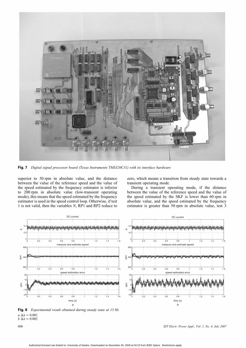
Fig. 7 Digital signal processor board (Texas Instruments TMS320C31) with its interface hardware
superior to 50 rpm in absolute value, and the distancebetween the value of the reference speed and the value ofthe speed estimated by the frequency estimator is inferiorto 200 rpm in absolute value (low-transient operatingmode), this means that the speed estimated by the frequencyestimator is used in the speed control loop. Otherwise, if test1 is not valid, then the variables N, RP1 and RP2 reduce to
606
Authorized licensed use limited to: University of Nantes. Downloaded on November 26, 2
zero, which means a transition from steady state towards atransient operating mode.
During a transient operating mode, if the distancebetween the value of the reference speed and the value ofthe speed estimated by the SKF is lower than 60 rpm inabsolute value, and the speed estimated by the frequencyestimator is greater than 50 rpm in absolute value, test 3
0 0.2 0.4 0.6 0.8 1 1.2 1.4 1.60
0.2
0.4
DC current
A
0 0.2 0.4 0.6 0.8 1 1.2 1.4 1.6850
900
950measure and estimate speed
rpm
0 0.2 0.4 0.6 0.8 1 1.2 1.4 1.6−20
−10
0
10
20speed estimation error
time (s)
a
rpm
0 0.2 0.4 0.6 0.8 1 1.2 1.4 1.60
0.2
0.4
DC current
A
0 0.2 0.4 0.6 0.8 1 1.2 1.4 1.6850
900
950measure and estimate speed
rpm
0 0.2 0.4 0.6 0.8 1 1.2 1.4 1.6−20
−10
0
10
20speed estimation error
time (s)
b
rpm
Fig. 8 Experimental result obtained during steady state at 15 Hz
a Dl ¼ 0.001b Dl ¼ 0.002
IET Electr. Power Appl., Vol. 1, No. 4, July 2007
009 at 04:23 from IEEE Xplore. Restrictions apply.

0 0.2 0.4 0.6 0.8 1 1.2 1.4 1.60
0.2
0.4
DC current
A
0 0.2 0.4 0.6 0.8 1 1.2 1.4 1.6850
900
950
1000
1050
1100measure and estimate speed
rpm
0 0.2 0.4 0.6 0.8 1 1.2 1.4 1.6−200
−150
−100
−50
0
speed estimation error
time (s)
rpm
DC current
0 0.2 0.4 0.6 0.8 1 1.2 1.4 1.60
0.2
0.4
A
measure and estimate speed
0 0.2 0.4 0.6 0.8 1 1.2 1.4 1.6850
900
950
1000
1050
1100
rpm
speed estimation error
time (s)
a b
0 0.2 0.4 0.6 0.8 1 1.2 1.4 1.6−200
−150
−100
−50
0
rpm
Fig. 9 Experimental result obtained during steady state at 15 Hz with þ20% of initial error
a Dl ¼ 0.001b Dl ¼ 0.002
1 1.01 1.02 1.03 1.04 1.05 1.06 1.07 1.08 1.09 1.1−0.02
−0.01
0
0.01
0.02output signal of the band−pass filter
A
1 1.01 1.02 1.03 1.04 1.05 1.06 1.07 1.08 1.09 1.1−1
−0.5
0
0.5
1x 10
−3 output signal of the double derivative filter
A (
rad/
s)2
time (s)
Fig. 10 Output signal of the two filters for a mechanical speed of600 rpm
IET Electr. Power Appl., Vol. 1, No. 4, July 2007
Authorized licensed use limited to: University of Nantes. Downloaded on November 26, 20
is valid. Therefore the steady state is reached and the vari-able N is incremented by 1 at each sample period. When thevariable N reaches the value of 2500 (after 0.5 s), the switchINT1 changes from position 0 to position 1 (Fig. 12). Thismeans that the frequency estimator is autonomous. In thisconfiguration, the used speed in the speed control loopalways comes from the SKF. If the machine is still insteady state after 1 s (N ¼ 5000), then the second logicalvariable RP2 is equal to 1 and the switch INT2 passesfrom position 0 to position 1. In this configuration, theused speed in the speed control loop comes from the fre-quency estimator. The static error between the referencespeed and the real mechanical speed is zero.
Fig. 14a represents the measured mechanical speed, 14bthe speed estimated by the SKF and 14c the speed estimatedby the frequency estimator with a load torque disturbance.The second section of Fig. 14a with the variables RP1and RP2 equal to 1 and 0, respectively, means that the
0 0.2 0.4 0.6 0.8 1 1.2 1.4 1.6
−0.2
0
0.2
0.4
DC current
A
0 0.2 0.4 0.6 0.8 1 1.2 1.4 1.60
500
1000
1500
2000measure and estimate speed
rpm
0 0.2 0.4 0.6 0.8 1 1.2 1.4 1.6−200
−150
−100
−50
0
50speed estimation error
time (s)
rpm
DC current
0 0.2 0.4 0.6 0.8 1 1.2 1.4 1.6
−0.2
0
0.2
0.4
A
measure and estimate speed
0 0.2 0.4 0.6 0.8 1 1.2 1.4 1.60
500
1000
1500
2000
rpm
speed estimation error
time (s)
a b
0 0.2 0.4 0.6 0.8 1 1.2 1.4 1.6−40
−20
0
20
40
rpm
Fig. 11 Experimental result obtained during speed variation
a Dl ¼ 0.001b Dl ¼ 0.002
607
09 at 04:23 from IEEE Xplore. Restrictions apply.

selection algorithm knows that the machine works in steadystate. After 1 s of steady state (between the instants 2 and3 s), the variables RP1 and RP2 are equal to 1. Thismeans that the machine is still in steady state and thespeed estimated by the frequency estimator is used in thecontrol loop.
We can also add the following:
1. The estimated speed by the frequency estimator is onlyused during the steady state and the low-transient operatingmode. The filter bandwiths can be reduced to 2 or 3 Hz inorder to decrease the variance upon the speed estimationwithout risk of divergence.2. During the transient state, the placement of the band-passfilter and the calculation of the coefficients of the FIR filterare made, thanks to the speed estimation by the SKF. Thishas some advantages.
(a) The tracking capability of the frequency estimator isincreased because the estimator is in open-loop.(b) The frequency estimator diverges when the speed ofrotation is low because it is not capable of extracting onlyone harmonic in the signal although the band-pass filterand the double derivative filter parameters are madewith the speed estimation by the SKF. Therefore theinjection of the speed estimation by the SKF allows
Fig. 12 Diagram of the selection algorithm
Fig. 13 Selection algorithm
Condition 2 is jvref2 vfj , 200 and jvfj . 50, condition 3 is jvref2vskfj , 60 rpm and jvfj . 50 rpm
608
Authorized licensed use limited to: University of Nantes. Downloaded on November 26, 2
the frequency estimator to converge very quickly to the‘exact’ value of the mechanical speed after a divergence.This is illustrated in Fig. 15.
Fig. 16a represents the measured mechanical speed, thespeed estimated by the SKF and the speed estimated bythe frequency estimator for a periodic speed referencechange from 600 to 2600 rpm. The selection algorithm
Table 3: Synthesis of the speed estimation selectedfollowing the operating mode of the DC-motor
Condition Stationary
Kalman filter
Frequency
estimator
steady state jvj � 50 rpm �
jvj � 50 rpm �
transient state jvref2 vj � 200 rpm �
jvref2 vj � 200 rpm �
Fig. 14 Experimental result obtained during a sensorless controlwith load torque disturbance
a Measure speedb Suboptimal kalman filter speed estimationc Frequency speed estimation
13 13.5 14 14.5 15 15.5 16−400
−300
−200
−100
0
100
200
300
400measure and estimate speed (frequency estimator)
rpm
time (s)
ω
ωf
convergence
divergence
critical zone
Fig. 15 Open-loop tracking capability of the frequencyestimator
IET Electr. Power Appl., Vol. 1, No. 4, July 2007
009 at 04:23 from IEEE Xplore. Restrictions apply.

0 2 4 6 8 10 12 14 16 18 20
−500
0
500
measure speed
rpm
0 2 4 6 8 10 12 14 16 18 20
−500
0
500
suboptimal Kalman filter speed estimation
rpm
0 2 4 6 8 10 12 14 16 18 20
−500
0
500
frequency speed estimation
rpm
time (s)
0 2 4 6 8 10 12 14 16 18 20−400
−200
0
200
400speed estimation error
rpm
8 8.5 9 9.5 10 10.5 11 11.5 12−20
−10
0
10
20zoom between 8 and 12 s
rpm
time (s)
a b
Fig. 16 Experimental result obtained during a sensorless control for a periodic speed reference change from 600 to 2600 rpm
5 10 15 20 25 30 35 40
0
200
400
600
measure and reference speed
rpm
5 10 15 20 25 30 35 40
0
200
400
600
speed estimation by suboptimal Kalman filter
rpm
5 10 15 20 25 30 35 40
0
200
400
600
speed estimation by frequency estimator
rpm
time (s)
a
0 5 10 15 20 25 30 35 40
−50
0
50
100
150
200
sledging error = reference speed − measure speed
rpm
time (s)
b
zero speed error
Fig. 17 Experimental result obtained during a sensorless control for a periodic speed reference change to 0–600 rpm
allows to make important changes of speed and allows zerotracking error at steady state (Fig. 16b).
Fig. 17a a shows a speed transient between 0 and600 rpm. Three important points can be seen in this figure.
1. The use of dependent parameter speed observer (here theSKF) leads to a bias estimation error (nearly 32 rpm atsteady state in this example) because parameters are notwell known and could fluctuate (see also Fig. 16b formore details).2. The use of frequency estimator leads to zero speed esti-mation error at steady state (see Fig. 17b between the instant5 and 10 s).3. On the other hand, high-transient behaviour can berealised with dependent parameter speed observer com-pared to frequency estimator.
Fig. 18 represents an experimental result obtained duringa sensorless control with an abrupt load torque disturbance.As we can see at the instant 3 s, the frequency estimatorcannot estimate the frequency of the harmonic at 16 times
IET Electr. Power Appl., Vol. 1, No. 4, July 2007
Authorized licensed use limited to: University of Nantes. Downloaded on November 26, 200
2 2.5 3 3.5 4 4.5 5 5.5
0
200
400
600
measure speed
rpm
2 2.5 3 3.5 4 4.5 5 5.5
0
200
400
600
suboptimal Kalman filter speed estimation
rpm
2 2.5 3 3.5 4 4.5 5 5.5
0
200
400
600
frequency speed estimation
rpm
time (s)
30 rpm statique error 0 rpm statique error
Fig. 18 Experimental result obtained during a sensorless controlwith an abrupt load torque disturbance
609
9 at 04:23 from IEEE Xplore. Restrictions apply.

the rotational frequency of the machine because of itsmedium tracking capability. In fact, this estimator is tunedso that the speed estimation is accurate in steady state(small variance), and so that the algorithm tracks theharmonic during low-transient operating modes. Thus, toreach high-transient behaviour and also zero speed estimationerror at steady state, we hold the plurality of the twoestimators.
5 Conclusion
The use of rotor slot harmonics for sensorless speed esti-mation is a difficult problem, notably because of thelocations of these harmonics towards power harmonics ofthe converter and the mechanical frequency oscillation.This approach is attractive because the speed estimator isnot parameter-dependent compared to standard techniquesbased on state space model. Experimental results showthat good tracking capabilities during transient and zerospeed error at steady state is ensured. This method is veryaccurate for some operating mode, so it is suitable forprecise feedback speed control. This allows us to concludethat our approach should be able to replace a mechanicalspeed sensor in a large variety of applications. Electricalpropulsion ship and traction railways could be an appli-cation field because of the slow-speed dynamique.Moreover, the frequency estimator could also be used incomplement of a low-cost mechanical sensor for fault-tolerant motor control to increase the reliability of thesystem. The impossibility to know the spin direction withthese methods can be pointed out. But this informationcan easily be found by a simple parameter-dependentspeed estimator. The computional cost of this speed estima-tor is reduced and allows to consider this algorithm as acomplementary speed estimator for a two spin directionhigh performance sensorless drive.
To reach high-transient behaviour and also zero speedestimation error at steady state, a commutator algorithm isproposed. This algorithm selects the best speed estimationaccording to the performance of the two speed estimatorsand the operating mode.
6 References
1 Vas, P.: ‘Sensorless vector and direct torque control’ (OxfordUniversity Press, 1998)
2 Zeraoulia, M., Benbouzid, M.E.H., and Diallo, D.: ‘Electric motordrive selection issues for HEV propulsion systems: a comparativestudy’, IEEE Trans. Vehicular Technol., 2006, 55, (6), pp. 513–518
3 Hilairet, M., Diallo, D., and Benbouzid, M.E.H.: ‘A self-reconfigurable and fault-tolerant induction motor controlarchitecture for hybrid electric vehicles’. Int. Conf. on ElectricalMachines (ICEM), September 2006
4 Leonhard, W.: ‘Control of electrical drives’ (Springer Verlag, 1985)
610
Authorized licensed use limited to: University of Nantes. Downloaded on November 26, 2
5 Chevrel, P., and Siala, S.: ‘Robust DC-motor speed controlwithout any mechanical sensor’. Proc. Electrimacs, Saint-Nazaire,September 1996
6 Sicot, L.: ‘Contribution a l’introduction de limitations dans les lois decommande de la machine synchrone a aimants permanents, approchetheorique et realisations experimentales, commande sans capteurmecanique’, PhD Thesis, l’Universite de Nantes, France, 1997
7 Trump, B.: ‘DC motor speed controller: control a DC motor withouttachometer feedback’ (Application Bulletin, Burr-Brown, 1999)
8 Leephakpreeda, T.: ‘Sensorless DC motor drive via optimalobserver-based servo control’, Optim. Control Appl. Methods, 2002,23, (5), pp. 289–301
9 Jaszczak, K., and Orlowska-Kowalska, T.: ‘Sensorless adaptive fuzzylogic control of DC drive with neural inertia estimator’, J. Electr.Eng., 2003, 3, (1)
10 Shen, J.X., Zhu, Z.Q., and Howe, D.: ‘Sensorless flux-weakeningcontrol of permanent magnet brushless machines usingthird-harmonic back-EMF’. IEEE Int. Electric Mach. Drives Conf.,IEMDC’03, 2003, vol. 2, pp. 1229–1235
11 Liu, Z.Z., Luo, F.L., and Rashid, M.H.: ‘Speed nonlinear control ofDC motor drive with field weakening’, IEEE Trans. Ind. Appl.,2003, 39, (2), pp. 417–423
12 Bowes, S.R., Sevinc, A., and Holliday, D.: ‘New natural observerapplied to speed-sensorless DC servo and induction motors’, IEEETrans. Ind. Electron., 2004, 51, (5), pp. 1025–1032
13 Li, S., Hai-Hiao, G., Watanabe, T., and Ichinokura, O.: ‘Sensorlesscontrol of DC motors based on extended observers’. 11th Int. PowerElectronics Motion Control Conf., EPE-PEMC, 2004, vol. 2,pp. 376–381
14 Ohishi, K., Nakamura, Y., Hojo, Y., and Kobayashi, H.:‘High-performance speed control based on an instantaneous speedobserver considering the characteristics of a dc chopper in a lowspeed range’, Electr. Eng. Jap., 2000, 130, (3), pp. 77–87
15 Hurst, K.D., and Habetler, T.G.: ‘Sensorless speed measurement usingcurrent harmonic spectral estimation in induction machine drives’,IEEE Trans. Power Electron., 1996, 11, (1), pp. 66–73
16 Hurst, K.D., Habetler, T.G., Griva, G., Profuno, F., Jansen, P.L.: ‘A selftuning closed-loop flux observer for sensorless control of inductionmachines’, IEEE Trans. Power Electron., 1997, 12, (5), pp. 807–815
17 Ferrah, A., Bradley, K.J., Hobenlaing, P.J., Woolfson, M.S., Asher,G.M., et al. ‘A speed identifier for induction motor drives usingreal-time adaptive digital filtering’, IEEE Trans. Ind. Appl., 1998,34, (1), pp. 156–162
18 Jansen, P.L., Corley, M.J., and Lorenz, R.D.: ‘Flux, position, andvelocity estimation in AC machines at zero and low speed viatracking of high frequency saliencies’, J. EPE, 1999, 9, (1–2),pp. 45–50
19 Degner, M.W., and Lorenz, R.D.: ‘Position estimation in inductionmachines utilizing rotor bar slot harmonics and carrier-frequencysignal injection’, IEEE Trans. Ind. Appl., 2000, 36, (3), pp. 736–742
20 Auger, F., and Hilairet, M.: ‘Suivi de raies spectrales avec un faiblecout de calcul’. Proc. Gretsi 99, September 1999, pp. 13–17
21 Regalia, P.A., Mitra, S.K., and Vaidyanathan, P.P.: ‘The digitalall-pass filter: a versatile signal processing building block’, Proc.IEEE, 1988, 76, (1), pp. 19–37
22 Auger, F.: ‘Introduction a la theorie du signal et de l’information –cours et exercices’ (Editions Technip, 1999)
23 Grewal, M.S., and Andrews, A.P.: ‘Kalman filtering, theory andpractice’ (Prentice Hall, Englewood Cliffs, NJ, 1993)
24 Brown, R.H., Schneider, S.C., and Mulligan, M.G.: ‘Analysis ofalgorithms for velocity estimation from discrete position versus timedata’, IEEE Trans. Ind. Electron., 1992, 39, (1), pp. 11–19
25 Hilairet, M., Auger, F., Ait-Ahmed, M., and Benkhoris, M.F.:‘Speed and position estimation from an absolute position encoder’.Proc. Electrimacs 99, Lisboa Portugal, September 1999, pp. 217–222
IET Electr. Power Appl., Vol. 1, No. 4, July 2007
009 at 04:23 from IEEE Xplore. Restrictions apply.