
Position-Sensorless Indirect Torque Control of Permanent ...
146
NTNU Norwegian University of Science and Technology Faculty of Information Technology and Electrical Engineering Department of Electric Power Engineering Isak Nordeng Jensen Position-Sensorless Indirect Torque Control of Permanent Magnet Synchronous Machines Master’s thesis in Energy and Environmental Engineering Supervisor: Roy Nilsen Co-supervisor: Alexey Matveev June 2021 Master’s thesis
-
Upload
khangminh22 -
Category
Documents
-
view
0 -
download
0
Transcript of Position-Sensorless Indirect Torque Control of Permanent ...

NTN
UN
orw
egia
n U
nive
rsity
of S
cien
ce a
nd T
echn
olog
yFa
culty
of I
nfor
mat
ion
Tech
nolo
gy a
nd E
lect
rical
Eng
inee
ring
Dep
artm
ent o
f Ele
ctric
Pow
er E
ngin
eerin
g
Isak Nordeng Jensen
Position-Sensorless Indirect TorqueControl of Permanent MagnetSynchronous Machines
Master’s thesis in Energy and Environmental EngineeringSupervisor: Roy NilsenCo-supervisor: Alexey Matveev
June 2021
Mas
ter’s
thes
is

Isak Nordeng Jensen
Position-Sensorless Indirect TorqueControl of Permanent MagnetSynchronous Machines
Master’s thesis in Energy and Environmental EngineeringSupervisor: Roy NilsenCo-supervisor: Alexey MatveevJune 2021
Norwegian University of Science and TechnologyFaculty of Information Technology and Electrical EngineeringDepartment of Electric Power Engineering


Abstract
Position-sensorless permanent magnet synchronous machine (PMSM) drives are emergingas the state-of-the-art in high-performance safety-critical and weight-sensitive applicationsdue to advantages such as high power and torque density, high efficiency and reliabilityand reduced hardware complexity, cost and size.
In this thesis, a state-of-the-art system-on-chip (SoC) based embedded controller is usedfor the development and implementation of C++ software that enables position-sensorlessindirect torque control (ITC) of PMSMs. Two fundamental-excitation based methodsfor sensorless control are developed and programmed on the SoC central processing unit(CPU) and verified using an embedded real-time simulator (ERTS) that is housed by theSoC field-programmable gate array (FPGA). Both methods utilize the active flux conceptfor rotor position estimation, but the means of which the active flux vector is obtained dif-fers between the two: The first method uses the Niemela-corrected voltage model, whilethe second method is based on the voltage-current model.
It is shown that an inaccurately estimated stator resistance results in a flux estimate thatdrifts and becomes increasingly inaccurate over time, which makes position-sensorless op-eration without the implementation of specialized flux models impossible. The proposedflux models both prove to be highly effective for sensorless operation with an erroneousresistance estimate in the medium and high speed region. Moreover, both models enablecrossing of the zero-speed region and persistent operation at very-low speeds below 0.1
per unit. Simulations are initially performed with a speed-dependent, quadratic load func-tion that is valid for the modelling of pumps and fans, but the models are also verified fora scenario where a constant load torque is applied, suggesting that they are applicable forconstant-load applications such as cranes and hoists.
The ERTS proves to be an immensely useful tool in the development of control softwarefor PMSM drives. The control software on the SoC processor is intended to drive eithera physical PMSM drive in a laboratory setup or the ERTS, and the latter enables the ver-ification of the sensorless control strategies without accessing an actual PMSM drive testbench. Owing to the real-time nature of the ERTS, due to the high processing capabilityof the FPGA, simulations can be drastically accelerated and control strategy verification ismade a less time-consuming effort than if conventional simulation tools were to be used.
i

Sammendrag
Sensorløse permanentmagnet synkronmotordrifter er i ferd med etablere seg som det fore-trukne valget for anvendelser som krever stor grad av sikkerhet, palitelighet og lav vekt.Dette kan tilskrives fordeler som høy effekt- og momenttetthet, virkningsgrad og palitelighetog redusert maskinvare-kompleksitet, kostnad og størrelse.
I denne avhandlingen blir en styringsplattform basert pa en ”system on chip” (SoC) bruktfor utvikling og implementering av C++-programvare som muliggjør sensorløs momentstyringav permanentmagnet synkronmaskiner. To metoder for sensorløs styring er implemenertog programmert pa SoC-prosessoren og verifisert ved hjelp av en sanntidssimulator som erintegrert i FPGAen pa SoCen. Begge metodene benytter seg av aktiv fluks-konseptet forrotorposisjon-estimering, men fremgangsmaten som benyttes for a estimere aktiv fluks-vektoren er ulik: Den første metoden benytter seg av den Niemela-kompenserte spen-ningsmodellen, mens den andre er basert pa spenning- og strøm-modellen.
Det blir demonstert at en unøyaktig estimert stator-resistans resulterer i et fluksestimatsom ”drifter” og blir unøyaktig over tid, noe som gjør sensorløs styring vanskelig. Beggefluksmodellene som benyttes viser seg a være høyst effektive for sensorløs styring medet unøyaktig resistans-estimat i medium- og høy-hastighetsomradet. Begge modellenemuliggjør kryssing av null-turtallsomradet, samt vedvarende kjøring ved lave turtall un-der 0.1 per unit. Simuleringene blir i utgangspunktet gjennomført med en hastighets-avhenging, kvadratisk lastfunksjon som brukes for modellering av pumper og vifter. Mod-ellene blir imidlertid ogsa verifsert for et scenario hvor en last med konstant moment blirbenyttet. Dette indikerer at metodene ogsa er gyldige for anvendelser som heiser og kraner.
Sanntidssimulatoren som har blitt benyttet har vist seg a være et nyttig verktøy i utviklin-gen og verifiseringen av styringsprogramvare for permanentmagnet synkronmotordrifter.Programvaren som har blitt utviklet kan anvendes pa en fysisk motordrift i et laborato-rie eller pa sanntidssimulatoren, og sistnevnte muliggjør testing av styringsprogramm-varen uten tilgang pa en fysisk testrigg. Som en følge av FPGAens høye prosessering-shastighet kan simulatoren gjennomføre simuleringer i sanntid, noe som gjør verifiseringav styringsstrategier en adskillig mindre tidkrevende prosess enn hvis konvesjoneller simu-leringsverktøy hadde blitt brukt.
ii

Preface
This thesis concludes my Master of Science degree in Energy and Environmental Engi-neering at the Norwegian University of Science and Technology, and is submitted to theDepartment of Electric Power Engineering. The thesis has been written in co-operationwith Alva Industries AS.
Working with this thesis has exposed me to a broad range of exciting fields within elec-tric power engineering, and has provided me with invaluable experience in conductingresearch and independently solving complex problems. There is however still much tolearn, and I am eager to keep exploring these realms as I enter the next stage of life andstart my professional career.
I would like to thank my supervisor, Professor Roy Nilsen, for his guidance and sup-port during the last academic year. His knowledge and vast experience within the field ofelectric motor drives have been an immense resource throughout this project. I also thankmy co-supervisor, Dr. Alexey Matveev at Alva Industries AS, for providing valuable in-sight into the world of electric motor manufacturing and the practical challenges that areencountered here.
During the course of this project, I have been fortunate enough to receive guidance andsupport from people who have chosen to share from their time despite lack of formal obli-gation to do so. Specifically, I extend my sincere thanks to Thomas Haugan for his helpwith setting up and becoming familiar with the software that has been used in this thesis,and Aravinda Perera, who in his doctoral thesis is working on a topic similar to the onethat is investigated in this master’s project. He has provided me with countless advice andshared from his knowledge across many fields, and in doing so, been a truly great supportduring the last months.
Last, but not least, I would like to thank my friends for making my time as a studentat NTNU a memorable experience, and my family for their tireless support.
iii

Trondheim, June 14, 2021
Isak Nordeng Jensen
iv

Table of Contents
Abstract i
Sammendrag ii
Preface iii
List of Figures xi
Nomenclature and Abbreviations xii
1 Introduction 11.1 Background . . . . . . . . . . . . . . . . . . . . . . . . . . . . . . . . . 11.2 Objective and Approach . . . . . . . . . . . . . . . . . . . . . . . . . . 31.3 Limitations . . . . . . . . . . . . . . . . . . . . . . . . . . . . . . . . . 31.4 Structure of Thesis . . . . . . . . . . . . . . . . . . . . . . . . . . . . . 4
2 Theoretical Background 52.1 The Permanent Magnet Synchronous Machine . . . . . . . . . . . . . . . 5
2.1.1 The Space-Vector Concept . . . . . . . . . . . . . . . . . . . . . 62.1.2 Dynamic Motor Model . . . . . . . . . . . . . . . . . . . . . . . 8
2.2 Control Principles . . . . . . . . . . . . . . . . . . . . . . . . . . . . . . 112.2.1 Existing Methods for Variable-Frequency Drives . . . . . . . . . 122.2.2 Indirect Torque Control of the PMSM . . . . . . . . . . . . . . . 13
2.3 Digital Control Implementation and Verification . . . . . . . . . . . . . . 172.3.1 Control Software Implementation: CPU Programming . . . . . . 172.3.2 Control Software Verification: The Embedded Real-Time Simula-
tor (ERTS) . . . . . . . . . . . . . . . . . . . . . . . . . . . . . 18
v
3 Position-Sensorless Indirect Torque Control of the PMSM 213.1 Stator Flux Linkage Estimation . . . . . . . . . . . . . . . . . . . . . . . 22
3.1.1 The Voltage Model . . . . . . . . . . . . . . . . . . . . . . . . . 22
3.1.2 The Current Model . . . . . . . . . . . . . . . . . . . . . . . . . 23
3.1.3 Steady-State Sensitivity of the Flux Models . . . . . . . . . . . . 23
3.2 Rotor Position and Speed Estimation . . . . . . . . . . . . . . . . . . . . 28
3.2.1 The Initialization Procedure . . . . . . . . . . . . . . . . . . . . 28
3.2.2 Operation Enabled: The Active Flux Concept . . . . . . . . . . . 28
3.3 On-Line Stator Voltage Estimation . . . . . . . . . . . . . . . . . . . . . 30
3.3.1 Non-Ideal Converters: Influence of Dead Time Effects . . . . . . 31
3.3.2 Estimating the Stator Voltage . . . . . . . . . . . . . . . . . . . . 32
3.4 Sensorless Operation Based on the Voltage Model . . . . . . . . . . . . . 33
3.4.1 Stator Flux Linkage Drifting . . . . . . . . . . . . . . . . . . . . 34
3.4.2 Stator Flux Linkage Drift Correction: The Niemela Method . . . 38
3.4.3 Modifying the Low-Pass Filter . . . . . . . . . . . . . . . . . . . 42
3.5 Sensorless Operation Based on the Voltage-Current Model . . . . . . . . 46
3.5.1 Using a Proportional Controller in the Feedback Loop . . . . . . 47
3.5.2 Using a Proportional-Integral Controller in the Feedback Loop . . 50
3.6 Possible Improvements of the Sensorless Control Schemes . . . . . . . . 52
3.6.1 Phase-Locked Loop for Rotor Position Estimate Filtering . . . . . 53
3.6.2 High Frequency Signal Injection for Standstill and Low-SpeedOperation . . . . . . . . . . . . . . . . . . . . . . . . . . . . . . 53
4 Real-Time Simulation Results 554.1 Sensorless Operation Without Drift Correction . . . . . . . . . . . . . . . 57
4.2 Sensorless Operation Based on the Niemela-Corrected Voltage Model . . 60
4.2.1 High-Speed Operation Including Start-Up . . . . . . . . . . . . . 60
4.2.2 Driving Through Zero-Speed . . . . . . . . . . . . . . . . . . . . 63
4.2.3 Very-Low Speed Operation . . . . . . . . . . . . . . . . . . . . . 65
4.2.4 Driving Through Zero-Speed With Constant Load Torque . . . . 69
4.3 Sensorless Operation Based on the Voltage-Current Model . . . . . . . . 71
4.3.1 High-Speed Operation Including Start-Up . . . . . . . . . . . . . 71
4.3.2 Driving Through Zero-Speed . . . . . . . . . . . . . . . . . . . . 73
4.3.3 Very-Low Speed Operation . . . . . . . . . . . . . . . . . . . . . 76
4.3.4 Driving Through Zero-Speed With Constant Load Torque . . . . 80
vi

5 Discussion 835.1 Comparison of the Performance of the Flux Models . . . . . . . . . . . . 835.2 General Remarks About Fundamental-Excitation Based Sensorless Control 855.3 The ERTS and Assessment of Result Validity . . . . . . . . . . . . . . . 86
6 Conclusion and Further Work 896.1 Conclusion . . . . . . . . . . . . . . . . . . . . . . . . . . . . . . . . . 896.2 Further Work . . . . . . . . . . . . . . . . . . . . . . . . . . . . . . . . 90
6.2.1 Software Verification on a Physical Laboratory Setup . . . . . . . 906.2.2 Improving the Performance of the Position-Sensorless Drive . . . 906.2.3 Further Testing of the Position-Sensorless Drive . . . . . . . . . 91
Bibliography 93
A The Inductance Matrix 99
B Motor Drive Data 101
C Base-Values Used for Per-Unit Conversion 103
D Scripts Used for Flux Model Sensitivity Analysis 105D.1 MATLAB Script for Voltage Model Sensitivity Analysis . . . . . . . . . 105D.2 MATLAB Script for Current Model Sensitivity Analysis . . . . . . . . . 108
E Current Model Parameter Sensitivity Analysis Results 113E.1 Impact of xd = 0.8xd . . . . . . . . . . . . . . . . . . . . . . . . . . . . 114E.2 Impact of xq = 0.8xq . . . . . . . . . . . . . . . . . . . . . . . . . . . . 115E.3 Impact of ψm = 0.8ψm . . . . . . . . . . . . . . . . . . . . . . . . . . . 116
F Phase-Locked Loop Filtering of the Position Estimate 117
G High-Frequency Signal Injection for Standstill and Low-Speed Operation 121
H C++ Control Software 123H.1 Voltage Estimation . . . . . . . . . . . . . . . . . . . . . . . . . . . . . 123H.2 The Current Model . . . . . . . . . . . . . . . . . . . . . . . . . . . . . 124H.3 The Voltage Model . . . . . . . . . . . . . . . . . . . . . . . . . . . . . 125H.4 Niemela-Correction . . . . . . . . . . . . . . . . . . . . . . . . . . . . . 126H.5 Position Estimation . . . . . . . . . . . . . . . . . . . . . . . . . . . . . 127
vii

viii

List of Figures
2.1 Permanent magnet synchronous machines with surface-mounted and interior-mounted permanent magnets. . . . . . . . . . . . . . . . . . . . . . . . . 6
2.2 Resulting current space-vector when the phase a current is at its maximumvalue. . . . . . . . . . . . . . . . . . . . . . . . . . . . . . . . . . . . . 8
2.3 Relationship between the different coordinate systems in a two-pole IPMSM. 102.4 Classification of a few commonly used control methods for variable fre-
quency drives. . . . . . . . . . . . . . . . . . . . . . . . . . . . . . . . . 122.5 Block diagram showing the general structure of the torque-controlled PMSM
drive. . . . . . . . . . . . . . . . . . . . . . . . . . . . . . . . . . . . . 142.6 The structure of the PMSM drive control software. Retrieved from [45]. . 182.7 The general structure of the SoC-based embedded controller. Retrieved
from [45]. . . . . . . . . . . . . . . . . . . . . . . . . . . . . . . . . . . 192.8 The embedded controller. . . . . . . . . . . . . . . . . . . . . . . . . . . 20
3.1 Error in flux estimate magnitude and angle and output torque due to anunderestimated stator resistance. . . . . . . . . . . . . . . . . . . . . . . 26
3.2 Error in flux estimate magnitude and angle and output torque due to a DCoffset in the stator voltage estimate. . . . . . . . . . . . . . . . . . . . . 27
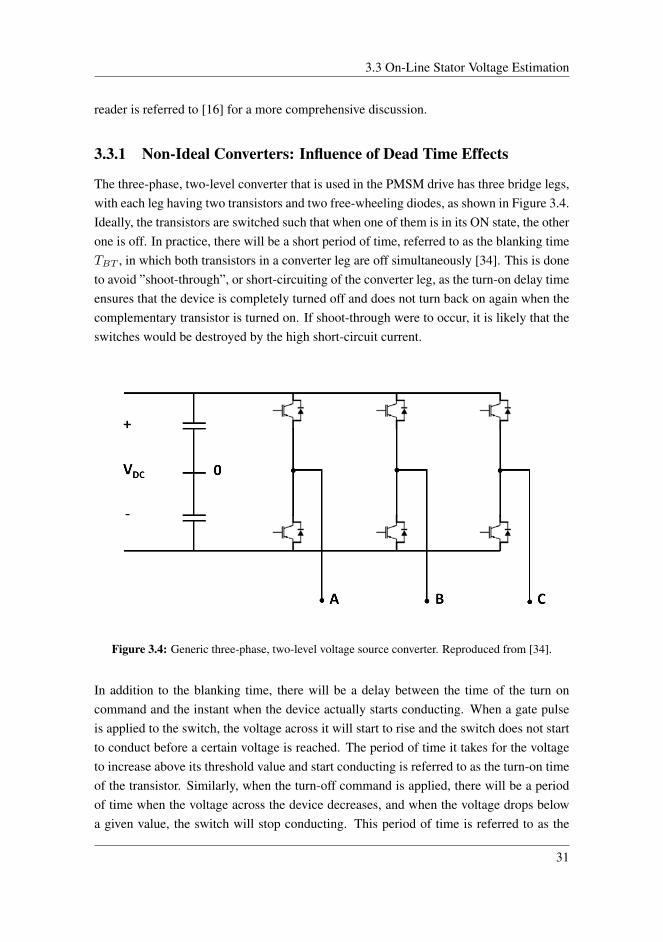
3.3 The active flux space vector. Reproduced from [40]. . . . . . . . . . . . . 293.4 Generic three-phase, two-level voltage source converter. Reproduced from
[34]. . . . . . . . . . . . . . . . . . . . . . . . . . . . . . . . . . . . . . 313.5 Ideal stator voltage, estimated stator voltage and stator current of phase a
of the motor. . . . . . . . . . . . . . . . . . . . . . . . . . . . . . . . . . 333.6 Real stator flux and flux estimate trajectories with erroneous initialization
of the voltage model. . . . . . . . . . . . . . . . . . . . . . . . . . . . . 35
ix

3.7 Voltage model flux estimate with erroneous initialization and voltage modelflux estimate with all quantities accurately estimated. . . . . . . . . . . . 36
3.8 Stator flux linkage drifting due to erroneous stator voltage and resistanceestimation. . . . . . . . . . . . . . . . . . . . . . . . . . . . . . . . . . . 37
3.9 Flux estimate magnitude squared, flux estimate magnitude squared andfiltered and the error signal. . . . . . . . . . . . . . . . . . . . . . . . . . 40
3.10 Low-pass filter time constant during start-up. . . . . . . . . . . . . . . . 41
3.11 Dynamics of the squared flux estimate, the squared and filtered flux esti-mate and the correction flux during a torque reference transient. . . . . . 43
3.12 The values of kT and kψ,corr during a torque reference step transient. . . 45
3.13 The voltage-current model with a proportional controller in the feedbackloop. Reproduced from [33]. . . . . . . . . . . . . . . . . . . . . . . . . 47
3.14 Response in the α-axis flux magnitude from the proportional controllerbased voltage-current model to a DC offset in the stator voltage. . . . . . 49
3.15 The voltage-current model with a proportional-integral controller in thefeedback loop. . . . . . . . . . . . . . . . . . . . . . . . . . . . . . . . . 50
3.16 Response in the α-axis flux magnitude from the proportional-integral con-troller based voltage-current model to a DC offset in the stator voltage.
. . . . . . . . . . . . . . . . . . . . . . . . . . . . . . . . . . . . . . . 51
4.1 Start-up and high speed operation without drift correction. . . . . . . . . 59
4.2 Start-up and high speed operation with the Niemela-corrected voltage model. 62
4.3 Driving through zero-speed with the Niemela-corrected voltage model. . . 64
4.4 . . . . . . . . . . . . . . . . . . . . . . . . . . . . . . . . . . . . . . . 65
4.5 Correction terms used in the Niemela-corrected voltage model when driv-ing through zero-speed. . . . . . . . . . . . . . . . . . . . . . . . . . . . 65
4.6 Start-up and very-low speed operation using the Niemela-corrected volt-age model. . . . . . . . . . . . . . . . . . . . . . . . . . . . . . . . . . . 66
4.7 Very-low speed operation with high initial speed, using the Niemela-correctedvoltage model. . . . . . . . . . . . . . . . . . . . . . . . . . . . . . . . . 68
4.8 Driving through zero-speed with constant load torque, using the Niemela-corrected voltage model. . . . . . . . . . . . . . . . . . . . . . . . . . . 70
4.9 Start-up and high speed operation using the voltage-current model. . . . . 73
4.10 Driving through zero-speed using the voltage-current model. . . . . . . . 75
4.11 Start-up and very-low speed operation using the voltage-current model. . 77
4.12 Very-low speed operation with high initial speed, using the voltage-currentmodel. . . . . . . . . . . . . . . . . . . . . . . . . . . . . . . . . . . . . 79
x

4.13 Driving through zero-speed with constant load torque, using the voltage-current model. . . . . . . . . . . . . . . . . . . . . . . . . . . . . . . . . 81
E.1 Error in flux estimate magnitude and angle and output torque due to anunderestimated d-axis reactance. . . . . . . . . . . . . . . . . . . . . . . 114
E.2 Error in flux estimate magnitude and angle and output torque due to anunderestimated q-axis reactance. . . . . . . . . . . . . . . . . . . . . . . 115
E.3 Error in flux estimate magnitude and angle and output torque due to anunderestimated permanent magnet flux linkage. . . . . . . . . . . . . . . 116
F.1 General structure of a phase-locked loop [18]. . . . . . . . . . . . . . . . 117F.2 Structure of the PI-controller based phase-locked loop. Reproduced from
[9]. . . . . . . . . . . . . . . . . . . . . . . . . . . . . . . . . . . . . . . 118
xi

Nomenclature and Abbreviations
List of Symbols
U = voltage [V]u = voltage [per unit]I = current [A]i = current [per unit]R = resistance [Ω]r = resistance [per unit]Ψ = magnetic flux linkage [Wb]ψ = magnetic flux linkage [per unit]L = inductance [H]T = torque [Nm]τ = torque [per unit]T = time constant [-]T = period [s]T = transformation matrix [-]J = moment of inertia [kgm2]
θ = electrical rotor position [] or [radians]N = speed [rpm]n = speed [per unit]p = number of pole pairs [-]X = reactance [Ω]x = reactance [per unit]F = MMF [A]S = apparent power [VA]f = frequency [Hz]j =
√−1 [-]
k = constant [-]H = transfer function [-]
xii

Subscripts
s = stator quantityr = rotor quantitya = phase a quantity, a-axis quantity, armature winding quantityb = phase b quantity, b-axis quantityc = phase c quantity, c-axis quantityα = α-axis quantityβ = β-axis quantityd = d-axis quantityq = q-axis quantitym = magnete = electromagneticl = loadn = nominalu = voltage model quantityi = current model quantitysamp = samplings = switchref = reference0 = initial valueLPF = low-pass filterPI = proportional-integral controllerf = field, filterfiltered = low-pass filtered quantitycorr = correction
Superscripts
s = quantity referred to statorr = quantity referred to rotorT = transpose
xiii

AbbreviationsVFD = variable-frequency drivePMSM = permanent magnet synchronous machineIPMSM = interior permanent magnet synchronous machineSPMSM = surface permanent magnet synchronous machineAC = alternating currentDC = direct currentFE = fundamental excitationHFSI = high-frequency signal injectionPWM = pulse width modulationMMF = magnetomotive forceEMF = electromotive forceDTC = direct torque controlITC = indirect torque controlVSC = voltage source converterMTPA = maximum torque per ampereSoC = system-on-chipSoM = system-on-moduleFPGA = field-programmable gate-arrayCPU = central processing unitERTS = embedded real-time simulatorPESC = power electronic systems and componentsPLL = phase-locked loopPI = proportional-integral
xiv

Chapter 1Introduction
1.1 Background
The world is currently undergoing a period of rapid change. The global energy demandis set to increase drastically over the course of the next years, and to mitigate climatechange as a result of greenhouse gas emissions, large-scale deployment of renewable en-ergy technologies is of the utmost importance [22]. The need for increased renewableenergy penetration is currently leading to a massive increase in the utilization of electricAC machines across many sectors of society, including industrial applications, power gen-eration, traction and transportation [6, 15]. Variable frequency drives (VFDs) play a majorrole in the shift towards a renewable energy-based society, as they are capable of provid-ing large energy savings through optimization of the operating speed of the AC machine[11, 7]. Permanent magnet synchronous machines (PMSMs) are currently becoming thepreferred machine type in many high-performance and weight-sensitive VFD applicationsdue to their high power and torque density, high efficiency, reliability, simple constructionand high fault-tolerance [30, 23].
Vector control is normally used in the control of modern PMSM drives in order to convertthe machine into an equivalent DC machine which has highly desirable control character-istics. Such a transformation requires accurate information about the position of the ma-chine rotor at all times [47, 28]. Traditionally, high-performance vector control of PMSMshave required the use of position sensors for rotor position extraction, but in recent years,position-sensorless PMSM drives have emerged as the state-of-the-art in safety-criticaltraction and automation applications. This is due to advantages such as increased reliabil-ity, reduced hardware complexity and cost, reduced size and lower maintenance require-
1

Chapter 1. Introduction
ments compared to conventional sensor-based PMSM drives [44, 19].
The available methods for position sensorless control of PMSMs, and variable-frequencydrives in general, can be divided into two main categories. These are fundamental-excitation(FE) based methods, which rely on the estimation of the back-EMF and stator flux linkageof the machine for position estimation, and saliency-tracking based methods that estimatethe rotor position through tracking of the spatial saliency of the machine [8, 52, 28]. Thefundamental-excitation based methods are in general best suited for medium and high-speed operation when the induced back-EMF is large, and during zero and low-speedoperation, such methods usually fail due to the lack of induced back-EMF. The saliency-tracking based methods, often referred to as high-frequency signal-injection (HFSI) basedmethods, work by injecting a high-frequency voltage signal on the top of the voltage fun-damental, while measuring the stator current response which contains information aboutthe spatial position of the rotor. The performance of such methods is thus independent ofthe motor speed and can hence be applied at standstill and very-low speeds. The accuracyof HFSI methods are usually related to the degree of saliency of the machine, however, andmay as such not be a viable option for low-saliency PMSM designs [31]. Drawbacks ofsignal-injection based methods are increased current and torque ripple, that may cause un-desirable vibration and acoustic noise, as well as increased complexity of the motor drivecontrol system [28]. Strategies where FE-based schemes and HFSI methods are combinedto achieve high performance across the complete speed range are presented in [51] and[44].
The development of motor drive control software has traditionally been done using phys-ical motor drive setups for software verification early in the design process [14]. Suchapproaches are often tedious and cumbersome, as they require access to a laboratory envi-ronment with a fully functioning test bench. Following the recent improvements in FPGAtechnology, the use of hardware emulators is emerging as a viable alternative to the phys-ical lab setups for control strategy verification [1, 21, 10]. Through the development ofsuch emulators, the physical behaviour of the motor drive can be replicated and controlsoftware can be verified by letting it drive the hardware emulator instead of the physi-cal motor drive. Such an FPGA-based emulator has recently been developed by the PowerElectronics Systems and Components (PESC) research group in the Department of ElectricPower Engineering at NTNU, and has been integrated in the department’s state-of-the-artsystem-on-chip based embedded controller. The control platform also houses a processingsystem where motor control software that drives either a physical motor drive or the hard-ware emulator can be implemented. The control platform is meant to provide a commonfoundation for further research within the field of electric motor drives and to serve as a
2

1.2 Objective and Approach
starting point for the thesis work of future master’s and PhD students.
1.2 Objective and Approach
The main aim of this thesis is to develop C++ subroutines that enable position-sensorlesscontrol a PMSM drive.
The following sub-objectives have been defined:
• Develop software that implements two separate fundamental-excitation based sen-sorless control strategies.
• Verify both strategies and control software using a PMSM drive hardware emulator.
• Provide a comparison of the aforementioned sensorless control strategies.
The thesis objectives will be accomplished using an approach based on the following se-quential steps:
1. Initially, a literature review that covers PMSM drive theory and sensorless controlconcepts are studied with the intention of becoming familiar with the theory that isrelevant for this project.
2. Next, sensorless control strategies will be developed and implemented in the em-bedded controller using the C++ programming language.
3. Finally, real-time simulation of the PMSM drive during position-sensorless opera-tion will be performed using the hardware emulator in order to validate the viabilityof the proposed methods.
1.3 Limitations
The work that is performed in this thesis is put under the following constraints:
• Only fundamental-excitation based methods for sensorless control will be consid-ered.
• Standstill operation of the motor will not be examined.
3

Chapter 1. Introduction
• The drive will be investigated during torque controlled operation only.
• The control software will not be verified on a physical PMSM motor drive, and thevalidation process will as such rely solely on the FPGA-based hardware emulator.
1.4 Structure of Thesis
This thesis consists of a total of 6 chapters:
Chapter 1 - Introduction contextualizes the work that is performed in this project, andcontains a presentation of the main thesis objectives, the approach that will be used andthe constraints the work will be put under.
Chapter 2 - Theoretical Background provides relevant background theory, includingpermanent magnet synchronous machine modelling, control principles and an introduc-tion to the control platform that will be used for implementation and verification of controlsoftware.
Chapter 3 - Position-Sensorless Indirect Torque Control of the PMSM is dedicatedto the description and discussion of the sensorless control strategies that are implementedin this thesis and the software development process.
Chapter 4 - Real-Time Simulation Results contains the real-time simulation results thatare obtained in order to verify the control software.
Chapter 5 - Discussion highlights the most important findings from the real-time sim-ulations and discusses their implications.
Chapter 6 - Conclusion and Further Work presents the most important conclusionsthat can be drawn from the work that is conducted in the thesis, as well as suggestions forfurther work.
4

Chapter 2Theoretical Background
This chapter presents the fundamentals of the theory that the work performed in this thesisis founded upon. A mathematical model of the ironless PMSM will be presented, alongwith the basics of the control strategy that will be implemented. Finally, the hardware andsoftware that will be used for control implementation and verification will be introduced.
The theory presented in this chapter is to some extent based on the theory presented inthe author’s specialization project that was written in the fall of 2020 [26]. It has howeverbeen revised, and significant modifications have been made to obtain the current version.
2.1 The Permanent Magnet Synchronous Machine
The permanent magnet synchronous machine (PMSM) is a type of synchronous machinein which the magnetic field excitation of the rotor is provided using permanent magnets.This allows for a simple, reliable and highly compact construction. Similarly to con-ventional syncronous machines, the stator of the machine contains three wye-connected,sinusoidally distributed windings that are identical and symmetrically displaced at 120
degrees. By supplying the stator windings with AC power using a three-phase power elec-tronics converter, the frequency of the stator currents can be varied through pulse-widthmodulation (PWM). This makes it possible to regulate the speed of the rotating magneticfield in the air gap of the machine, and hence the speed of the rotor. This is the mainprinciple of operation of PMSM-based variable frequency drives.
5

Chapter 2. Theoretical Background
There are in general two main ways of mounting the permanent magnets on the rotor of themachine, as shown in Figure 2.1. The placement of the permanent magnets will affect thebehaviour and the characteristics of the machine. A machine with surface-mounted per-manent magnets yields the simplest construction, but the rotor magnets will in this case beprone to mechanical stress. If the permanent magnets are interior-mounted, the mechanicalstress on the magnets will reduce and durability of the machine may increase. A conse-quence of interior-mounted magnets is that the machine becomes salient, meaning that thed- and q- axis inductances are unequal, which results in the generation of reluctance torque.This is due to the fact that the permanent magnets have a relative permeability that for allpractical purposes can be assumed to be equal that of air. The concept of the dq coordinatesystem will be explained in detail later in this chapter. From Figure 2.1, it is evident thatthe air gap of the machine becomes larger in the case of surface-mounted magnets. Thisresults in lower machine inductances, which gives a machine with fast speed response, butalso large current ripple which may cause undesirable torque and speed pulsations.
(a) SPMSM (b) IPMSM
Figure 2.1: Permanent magnet synchronous machines with surface-mounted and interior-mountedpermanent magnets.
2.1.1 The Space-Vector Concept
Modelling and control of electrical machines usually requires utilization of space vectors.In 1959, the space vector concept for multi-phase machines was developed by Kovacs andRacz and presented in [29]. They proposed to represent multi-phase machine quantitiesas a single vector variable, and in doing so, they laid the foundation of vector control ofvariable-frequency drives.
The concept can be demonstrated by considering the magnetomotive force (MMF) in theair-gap of the PMSM resulting from the stator phase currents. The MMF is a function ofthe instantaneous value of the phase currents ia(t), ib(t) and ic(t), as well as the angle
6

2.1 The Permanent Magnet Synchronous Machine
displacement with respect to the a axis, θ, and is given by the following expression [36]:
F (θ, t) = N
[ia(t) cos (θ) + ib(t) cos
(θ − 2π
3
)+ ic(t) cos
(θ +
2π
3
)](2.1)
Here, N is the effective number of turns per winding. If one defines the unit vectors a, band c to point in the direction of the winding axes, the MMF can be rewritten as a vectorquantity, or a space vector, as shown below:
F (t) = N [ia(t) · a+ ib(t) · b+ ic(t) · c]
= N [ia(t) + ib(t) + ic(t)]
= F a(t) + F b(t) + F c(t)
(2.2)
In Equation 2.2, the phase current space vectors ia(t), ib(t) and ic(t) have been introducedand the resultant air-gap MMF space vector has been expressed as the sum of the MMFspace vector for each of the phases. Similarly, the resultant stator current space vector canbe defined as
iss(t) = ia(t) + ib(t) + ic(t) =
ia(t)
ib(t)
ic(t)
(2.3)
Space vectors for stator voltages and flux linkages can be defined in a similar manner,and all three-phase machine variables can hence be represented as vector quantities in thetwo-dimensional vector space. This concept is fundamental for the development of themathematical model of the machine that will be presented in the next section, and forms abasis for the concept of vector control that will be presented later in this thesis.
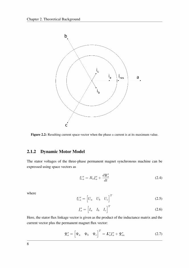
Figure 2.2 illustrates the space-vector concept. Here, the resulting current space vectorwhen the phase a current is at its maximum value is displayed.
7
Chapter 2. Theoretical Background
Figure 2.2: Resulting current space-vector when the phase a current is at its maximum value.
2.1.2 Dynamic Motor Model
The stator voltages of the three-phase permanent magnet synchronous machine can beexpressed using space vectors as
Uss = RsIss +
dΨss
dt(2.4)
whereUss =
[Ua Ub Uc
]T(2.5)
Iss =[Ia Ib Ic
]T(2.6)
Here, the stator flux linkage vector is given as the product of the inductance matrix and thecurrent vector plus the permanent magnet flux vector:
Ψss =
[Ψa Ψb Ψc
]T= LssI
ss + Ψs
m (2.7)
8
2.1 The Permanent Magnet Synchronous Machine
Both the inductance matrix, Lss, and the permanent magnet flux linkage are dependent onthe rotor position. The inductance matrix is presented in Appendix A, while the permanentmagnet flux linkage vector is given as
Ψsm = Ψm
cos (θ)
cos (θ − 2π3 )
cos(θ + 2π3 )
(2.8)
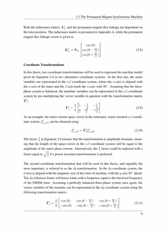
Coordinate Transformations
In this thesis, two coordinate transformations will be used to represent the machine modelgiven by Equation 2.4 in two alternative coordinate systems. In the first one, the statorvariables are represented in the αβ coordinate system, where the α-axis is aligned withthe a-axis of the stator and the β-axis leads the α-axis with 90. Assuming that the three-phase system is balanced, the machine variables can be represented in the αβ coordinatesystem by pre-multiplying the vector variable in question with the transformation matrixT ss:
T ss =
2
3
[1 − 1
2 − 12
0√
32 −
√3
2
](2.9)
As an example, the stator current space vector in the stationary, stator-oriented αβ coordi-nate system, Iss,αβ , can be obtained using
Iss,αβ = T ssIss,abc (2.10)
The factor 23 in Equation 2.9 ensures that the transformation is amplitude invariant, mean-
ing that the length of the space-vector in the αβ coordinate system will be equal to theamplitude of the stator phase current. Alternatively, the 2
3 factor could be replaced with a
factor equal to√
23 if a power invariant transformation is preferred.
The second coordinate transformation that will be used in this thesis, and arguably themost important, is referred to as the dq transformation. In the dq coordinate system, thed-axis is aligned with the magnetic axis of the rotor of machine, with the q-axis 90 ahead.The dq reference-frame will hence rotate with a frequency equal to the electrical frequencyof the PMSM rotor. Assuming a perfectly balanced three-phase system once again, thevector variables of the machine can be represented in the dq coordinate system using thefollowing transformation matrix:
T rs =
2
3
[cos (θ) cos (θ − 2π
3 ) cos (θ + 2π3 )
− sin (θ) − sin (θ − 2π3 ) − sin (θ + 2π
3 )
](2.11)
9

Chapter 2. Theoretical Background
The stator current space vector represented in the rotating, rotor-oriented dq coordinatesystem, Irs, is now given by
Irs = T rsIss (2.12)
Figure 2.3 illustrates the relationship between the three different coordinate systems in thecase of a two-pole PMSM with interior-mounted magnets. The αβ-coordinate system isrepresented by the red axes, while the dq-coordinate system is represented by the blueaxes. The α-axis is seen to correspond with the a-axis of the stator, while the d-axis inthe rotor-oriented coordinate systems coincides with the magnetic axis of the rotor. Theelectrical rotor position, θ, is equal to the displacement of the d-axis with respect to thea-axis.
Figure 2.3: Relationship between the different coordinate systems in a two-pole IPMSM.
The Transformed, per unit Scaled Motor Model
If the motor model given by Equation 2.4 is transformed to the dq coordinate system, asimplified motor model is obtained. The PMSM can now be modelled as a two-phasemotor with DC stator quantities in steady state and a simplified motor inductance matrixthat has become independent of the rotor position. To ensure that any overloading of the
10

2.2 Control Principles
machine can be easily detected, as well as to make it easier to compare individual machinesand to reuse motor control software, the motor model quantities are scaled by their basevalues to obtain an equivalent per unit model. The dynamic per unit model of the IPMSMin the rotor-oriented dq coordinate system that will be used to implement vector control ofthe motor is given by
urs = rsirs +
1
ωn
dψrs
dt+ njψr
s(2.13)
whereurs =
[ud uq
]T(2.14)
irs =[id iq
]T(2.15)
j =
[0 −1
1 0
](2.16)
The stator flux linkage vector is now given by
ψrs
=[Ψd Ψq
]T= xrsi
rs + ψr
m(2.17)
where
xrs =
[xd 0
0 xq
](2.18)
ψrm
=[ψm 0
]T(2.19)
In Equation 2.13, n is the per unit electrical speed and ωn is the nominal angular frequency.
The torque output of the machine can be found using
τ = ψdiq − ψqid = ψmiq − (xq − xd)idiq (2.20)
2.2 Control Principles
In this section, an overview over some commonly used methods for control of AC ma-chines will be presented, along with a more detailed discussion of the Indirect TorqueControl (ITC) method that will be employed in this thesis.
11

Chapter 2. Theoretical Background
2.2.1 Existing Methods for Variable-Frequency Drives
The control of variable-frequency drives can generally be divided into two main categories.These are scalar control methods, in which scalar motor quantities are being controlled,and vector control methods, that are based on controlling both the magnitude and angleof space-vector motor quantities. The chart in Figure 2.4 gives an overview over a fewcommonly used control methods for variable-frequency motor drives.
Figure 2.4: Classification of a few commonly used control methods for variable frequency drives.
The most common scalar control method is the volts-per-hertz (V/f ) control method.Here, the ratio between the magnitudes of the stator voltage and the frequency of themachine is kept constant, resulting in the stator flux linkage, and hence motor torque,being maintained at rated value across the whole speed range. This method is mostlyused to control induction motors, but has also been shown to be effective in conventionalPMSM drives [12, 46]. The V/f method is an open-loop control method, which makeshigh-performance control difficult. It is however very simple, making implementation un-complicated and control hardware requirements low.
With the increasing computational power of microprocessors, vector control methods havebecome dominant in variable-frequency drives applications. In the 1960s, the IndirectTorque Control (ITC) method, often referred to as vector control or field-oriented control,was introduced as a result of the desire to control three-phase machines in a way similarto the DC machine. In the DC machine, the flux and the torque can be controlled inde-
12

2.2 Control Principles
pendently by changing the field and the armature current, respectively. In [5], Blaschkesuggested a control method based on the transformed model of the synchronous machinethat was presented in Section 2.1.2, in which the d-axis of the the d− q reference frame isaligned with the rotor magnetic axis. Using this approach, the stator current space vectorwas decomposed into a field-producing component, id, and a torque-producing compo-nent, iq , that corresponded with the field and armature current of the DC machine, respec-tively. By changing the d and q axis currents of the machine, the output torque of themachine could be controlled indirectly. The ITC method will be employed in this theses,and a more thorough discussion of this method is therefore presented in Section 2.2.2.
In the mid-1980s, a new method for controlling AC machines was developed. In [48],Takahashi and Noguchi proposed a control method in which the torque and stator flux ofthe machine were controlled directly using hysteresis controllers. This method was latertermed the Direct Torque Control (DTC) method. Almost simultaneously, Depenbrockpresented a similar method in [13]. Depenbrock called his method Direct Self Control(DSC), and today, the DTC control method is usually credited to all three individuals. TheDTC used the voltage model that will be presented in Section 3.1.1 for estimation of thestator flux, while the current model that is discussed in Section 3.1.2 was used for correc-tion of the voltage model flux estimate. Once the stator flux was estimated, the torque ofthe machine could be calculated as the cross product of the estimated flux and the statorcurrent. The estimated stator flux and torque were then compared to their reference val-ues using hysteresis controllers, and the outputs of the controllers were used to obtain avoltage reference vector that determined the switching order of the converter switches.
2.2.2 Indirect Torque Control of the PMSM
As mentioned in the previous section, the goal of the Indirect Torque Control method wasto enable control of AC machines in a way that resembled the control of DC machines. Inthe DC machine, the electromagnetic torque, τ , is proportional to the product of the fieldwinding flux linkage, ψf , and the armature current, ia, as shown in Equation 2.21. If thefield current, and hence also field flux, is held constant, the electromagnetic torque caneasily be controlled by changing the armature current of the machine.
τ ∝ ψf ia (2.21)
A similar expression for the electromagnetic torque output of the PMSM was presented inEquation 2.20, and is repeated below:
τ = (ψm − (xq − xd)id)iq (2.22)
13

Chapter 2. Theoretical Background
By comparing Equation 2.21 and Equation 2.22, it can be seen that the PMSM torqueequation is analogous to the DC machine torque equation. Here, the field flux given byψm − (xq − xd)id corresponds to ψf in the DC machine, and can be controlled by reg-ulating the d-axis current. If the value of this term is held constant, the torque output ofthe machine can easily be controlled by regulating iq , which corresponds to ia in the DCmachine.
An overview of the indirect torque-controlled PMSM drive is displayed in Figure 2.5. Thed- and q-axis reference currents are calculated based on the torque reference and comparedwith the measured stator currents. The difference between reference values and measuredvalues is passed to a PI controller that is tuned using modulus optimum, as explained in[37]. A feed-forward decoupling term is added to the output of the PI controller in orderto eliminate the d- and q-axes cross-coupling and obtain the converter voltage referencesin the rotor oriented reference frame. Next, voltage references in the stator-oriented ref-erence frame are obtained by performing an αβ-transformation. These are passed to thepulse-width modulator that generates the gating signals for the voltage source converterthat feeds the stator windings of the PMSM. The αβ and dq transformations require therotor position, θ, and the decoupling term calculator requires the rotor speed, n. Methodsfor estimation of these quantities will be presented later in the thesis.
Figure 2.5: Block diagram showing the general structure of the torque-controlled PMSM drive.
14

2.2 Control Principles
Maximum-Torque-Per-Ampere Control
A common ITC strategy is to orient the stator current vector in a way that maximizes theoutput torque of the machine for the given current magnitude. If the PMSM is non-salient,the reluctance along the flux paths of the d and q axis are equal, resulting in equal d and qaxis inductances. The torque equation of the machine then reduces to
τ = ψmiq (2.23)
From Equation 2.23, it can be seen that the output torque is directly proportional to theq-axis component of the stator current, and the maximum amount of torque for a givencurrent magnitude is therefore generated if the current space vector is aligned with the q-axis of the dq reference system. This is done by applying the following current references:
id,ref = 0 (2.24)
iq,ref =τe,refψm
(2.25)
Here, τe,ref is the torque reference. If the PMSM has interior-mounted permanent mag-nets, however, the output torque will be given by Equation 2.22. Since magnets haveapproximately the same relative permeability as air, the inductance along the d-axis willbe lower than along the q-axis of the motor. From Equation 2.22 it can be seen that if anegative d axis current is applied, this difference in inductance can be used to generate anadditional torque component, usually referred to as reluctance torque. For PMSMs withinterior-mounted magnets, it is therefore desirable to operate the machine with a negatived-axis current in order to utilize this reluctance torque. As there is an infinite number of d-and q-axis currents that will produce the same torque, finding the combination that givesthe maximum torque output per ampere for this machine type becomes an optimizationproblem. This problem was first analyzed in [24], where Jahns et al. developed analyticalexpressions that can be used to obtain the optimal combination of d- and q-axis current.The current references in this thesis will be calculated based on the expressions in Equation2.26 and Equation 2.27 [45].
id,ref =
ψm
3 −3
√(ψm
3 )3 +(xq−xd)2τ2
e,ref
3ψm
xq − xd(2.26)
iq,ref =τe,ref
ψm − (xq − xd)id(2.27)
With the maximum torque per ampere control method properly implemented, the stator
15

Chapter 2. Theoretical Background
current that is necessary for a given torque output is minimized. As the copper lossesof the machine are proportional to the square of the stator current, this control strategyminimizes copper losses and maximizes the efficiency of the machine. Additionally, byreducing the stator current magnitude, the size of the converter can be reduced. Hence,the cheapest converter for a given torque is obtained when maximum-torque-per-amperecontrol is implemented.
Field-Weakening
When the motor operates at rated speed, the back-EMF of the machine, given as the prod-uct of stator flux linkage and motor speed, will have become equal to the rated statorvoltage. The rated stator voltage corresponds to the maximum output voltage of the con-verter, which means that the converter has saturated and is not able to increase its outputvoltage further. At this operating point, no current is flowing into the stator windings,making acceleration beyond the rated speed impossible. To enable operation above speedsof 1 per unit, one must therefore start to decrease the stator flux as the motor approachesrated speed. This way, the back-EMF is not exceeding the rated stator voltage, allowingthe machine to accelerate further.
The per unit stator flux linkage in the dq-coordinate system is given by
ψd = xdid + ψm (2.28a)
ψq = xqiq (2.28b)
As previously discussed, it is desirable to maintain the q-axis current as large as possible,and field-weakening should therefore be performed by applying a negative d-axis cur-rent that counteracts the magnetic field from the permanent magnets. From the equationsabove, it is however obvious that the stator flux linkage reduction that can be obtaineddepends on the magnitude of the d-axis reactance. If a large field-weakening region isrequired, the inductance along the d-axis flux path of the machine must therefore be large.For a PMSM with saliency, this will reduce the reluctance torque generation, and hencecome at the cost of the torque production capability of the machine. For low-inductancemachines, a large negative d-axis current must be applied in order to achieve a notablestator flux reduction. The cost of applying a d-axis current is a corresponding reduction ofthe q-axis component, as a constant current space vector magnitude must be maintained.Due to the magnitude of the d-axis current that must be applied, field-weakening in low-inductance machines will therefore lead to a large reduction in the q-axis current and hencealso the torque output of the machine. Field-weakening in such machines might thereforenot be justifiable.
16

2.3 Digital Control Implementation and Verification
2.3 Digital Control Implementation and Verification
The sensorless control algorithms that are developed in this thesis will be implementedand verified using the PicoZed 7030 system-on-module (SoM) from Avnet. The SoM isbased on the Zynq 7030 system on chip (SoC), that contains two ARM Cortex-A9 cen-tral processing units (CPUs) and one field-programmable gate array (FPGA). One of theon-chip processors runs a Linux program that is used for monitoring and programming ofthe remaining processor and the FPGA, while the second on-chip processor can be pro-grammed with the C++ programming language, using the Xilinx Software DevelopmentKit (XSKD). This is where the control strategies and algorithms that are developed in thisthesis will be implemented.
The hardware of a complete permanent magnet synchronous motor drive has been pro-grammed on the FPGA on the SoC to produce an embedded real-time simulator (ERTS)that is capable of emulating the PMSM drive. The control software that is implementedin the processor is intented to drive either the emulated drive in the ERTS or a physicalPMSM drive. In this thesis, the control software that is developed will be verified usingthe ERTS. The development of the ERTS and the processor control algorithms has been anongoing effort in the Power Electronic Systems and Components (PESC) research groupin the Department of Electric Power Engineering over the last few years, and at least twomaster’s theses have been dedicated to this purpose [16, 35]. A detailed description of thecontrol platform and an analysis of the performance of the ERTS is provided by Perera etal. in [45]. The embedded controller is pictured in Figure 2.8.
2.3.1 Control Software Implementation: CPU Programming
The on-chip processor of the control platform contains the majority of the control softwarethat is necessary to operate a PMSM drive when this thesis is initiated, with functional-ity such as per unit scaling, reference frame transformations, maximum-torque-per-ampereand field-weakening strategies and indirect torque control algorithms already implemented[45]. However, the control software relies on the measuring of the rotor position and speed,and is as such not capable of driving the PMSM without the use of a position-sensor. Asstated in Chapter 1, the main objective of this thesis is to develop sensorless control sub-routines which shall be added to the existing control software library that is programmedon the on-chip processor.
The control software is written using the C++ programming language, which due to its
17

Chapter 2. Theoretical Background
object-oriented nature ensures scalability, flexibility and structure of the control software.The control software is structured in different layers, as shown in Figure 2.6, where in-formation is passed only between neighbouring layers. The flux modelling and positionand speed estimation software that this thesis contributes with will be written in the drivesoftware layer (layer 2).
Figure 2.6: The structure of the PMSM drive control software. Retrieved from [45].
2.3.2 Control Software Verification: The Embedded Real-Time Sim-ulator (ERTS)
The control software development process in this thesis will rely on the use of the ERTSfor verification and validation. In the past, motor control strategies have usually been de-veloped and tested on a physical motor drive in a lab environment, but the recent trend isto perform software testing and verification using simulated motor drive models [14, 1].This is referred to as software-in-the-loop (SIL) testing, and requires accurate emulationof the physical behaviour of the motor drive.
The ERTS that is used in this thesis is implemented through the integration of a seriesof building blocks that are programmed on the FPGA and emulate the different hardwarecomponents of the drive, such as the voltage-source converter, the PMSM, the mechanicalload etc. Due to the large processing capability of the FPGA, the motor model equationscan be solved during time-steps that is equal to the real-world clock, yielding a simulatorthat is capable of emulating the motor drive in real-time [39]. This means that a simulationwith a duration of 1 second can be performed over a time period of 1 second, and simu-lation results can be obtained much faster than if conventional simulation tools such asMATLAB Simulink are used. The emulator is interfaced with the CPU on the SoC, whichmeans that the control software that is implemented here can be used to drive the ERTSif a physical motor drive is not available. There are hence two main advantages of usingthe ERTS in the control algorithm development process: Control strategies can be tested
18
2.3 Digital Control Implementation and Verification
through real-time simulation, making it a significantly less time-consuming effort than ifconventional simulation tools are used, and the ERTS enables software-in-the-loop test-ing, which makes a physical motor drive redundant in the control software developmentprocess.
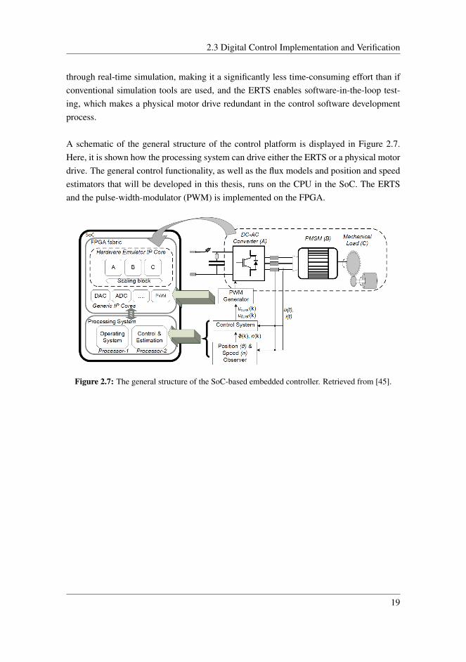
A schematic of the general structure of the control platform is displayed in Figure 2.7.Here, it is shown how the processing system can drive either the ERTS or a physical motordrive. The general control functionality, as well as the flux models and position and speedestimators that will be developed in this thesis, runs on the CPU in the SoC. The ERTSand the pulse-width-modulator (PWM) is implemented on the FPGA.
Figure 2.7: The general structure of the SoC-based embedded controller. Retrieved from [45].
19

Chapter 2. Theoretical Background
Figure 2.8: The embedded controller.
20

Chapter 3Position-Sensorless Indirect TorqueControl of the PMSM
Indirect torque-control of electric machines is accomplished by controlling the stator cur-rents in the rotor-oriented reference frame, and knowledge about the rotor position is there-fore necessary for its implementation. Traditionally, the rotor position has been obtainedusing position sensors such as encoders or resolvers. However, the current trend in elec-tric machine drives is to avoid any position or speed sensors by obtaining these quantitiesthrough estimation. By removing position and speed sensors, the cost and complexity ofthe drive can be greatly reduced, resulting in increased reliability and lower maintenancerequirements. Additional benefits are reduced weight and size.
With sensors removed, the main obstacle in any sensorless motor drive is obtaining suf-ficiently accurate estimates of the rotor position and speed. Over the years, various esti-mation methods have been proposed. Generally, these methods fall within one of of thefollowing categories: Fundamental-excitation based methods, that relies on the back-EMFof the machine for position estimation, and saliency tracking methods, that work by in-jecting high-frequency voltage components in the stator and extracting the rotor positionfrom the response in the stator current. In this thesis, fundamental-excitation based sen-sorless control methods will be considered. These estimate the rotor position and speedthrough a series of two steps: First, the stator flux linkage space vector is estimated usingthe back-EMF of the machine. Then, the flux estimate is used to obtain estimates of therotor position.
21

Chapter 3. Position-Sensorless Indirect Torque Control of the PMSM
3.1 Stator Flux Linkage Estimation
Rotor position estimation in fundamental-excitation based sensorless motor drives startswith obtaining the stator flux linkage of the machine, and accurate models for flux esti-mation thus becomes essential in any high-performance motor drive. There are two mainmodels that can be used to identify the stator flux vector based on the PMSM motor model.These are referred to as the voltage model and the current model, and will be presented inthis section.
3.1.1 The Voltage Model
The voltage model for flux estimation is based on the stator voltage balance equations thatwas presented in Section 2.1. By re-writing the per unit equivalent of Equation 2.4, theback-EMF of the motor in the stationary stator-oriented reference can be written as
dψss
dt= uss − rsiss (3.1)
The voltage model provides an estimate for the stator flux linkage in the stator-orientedαβ reference frame by integrating the stator back-EMF according to Faraday’s law ofinduction, as shown in Equation 3.2
ψss
= ψss0
+ ωn
∫ t
0
(uss − rsiss)dt (3.2)
Here, ψs0
is the initial value of the stator flux. The discrete-time equivalent of Equation3.2 is given by
ψss[k] = ψs
s[k − 1] + ωn · Tsamp · (uss[k]− rsiss[k]) (3.3)
Generally, the voltage model does not perform well at low speeds. When the speed iszero or close to zero, the back-EMF of the machine becomes very small, which will resultin inaccurate flux estimates. While sensorless operation based on the voltage model is aviable option if the low-frequency range is exceeded rapidly, continuous operation at zeroor close to zero speed is therefore impossible. The voltage model is thus best suited forflux estimation in the medium and high speed range. It will later be shown that the fluxestimates might become inaccurate even for high frequencies if the inputs to the voltagemodel deviate from their ideal values, and methods that compensate these inaccuraciesand stabilize the flux estimate are therefore always necessary in practical applications.
22

3.1 Stator Flux Linkage Estimation
3.1.2 The Current Model
The second model for flux identification that will be considered in this thesis is referred toas the current model. In this model, the measured stator currents along with the machineinductances are used to provide estimates of the stator flux, as shown in Equation 3.4.
ψrs
= xrsirs + ψr
m(3.4)
The discrete-time equivalent of the current model becomes
ψrs[k] = xrsi
rs[k] + ψr
m(3.5)
In contrary to the voltage model, flux estimation using the current model is done in therotor-oriented dq reference frame. This means that the rotor position is required as an inputto the model, and the current model alone can therefore not be used to estimate the rotorposition during sensorless operation. Assuming that an accurate position measurement isavailable and that the stator inductances and permanent magnet flux linkage are known,the current model will produce an accurate flux estimate across the whole speed range. Inthis thesis, the current model will be used to initialize the voltage model flux estimate oncethe rotor of the machine has been rotated into a known initial position before start-up. Itwill also be showed that the current model can be used in tandem with the voltage modelto produce a stable, closed-loop flux observer.
3.1.3 Steady-State Sensitivity of the Flux Models
The flux models that were presented in the preceding sections are highly sensitive to varia-tions in the values of the motor parameters rs, xd, xq and ψm. Although motor parametervalues usually are provided by the manufacturer, these are only valid in certain operat-ing points and should only be considered estimates. In practice the exact values of themotor parameters will depend on current operating conditions, such as loading, ambienttemperature, frequency and magnetic saturation. Motor inductances are mainly dependenton magnetic saturation, and will hence be influenced by the motor loading. ψm and rs areon the other hand to a greater extent temperature dependent, making them vulnerable tovariations in loading as well as ambient temperature. [42, 43]
In addition to erroneously estimated motor parameters, inaccurate information about thestator voltage and current may also contribute to imperfect flux estimation. Usually, thestator currents of the motor are measured using current sensors, and in this thesis, it willbe assumed that they are accurately measured at all times. The stator voltage, on the otherhand, is often estimated. The most common way of doing so is to use the reference voltage
23

Chapter 3. Position-Sensorless Indirect Torque Control of the PMSM
of the converter. If the non-linear voltage drops across the converter are modelled, theycan be subtracted from the reference voltage and an estimate for the actual stator voltagecan be obtained. This method will be analyzed in more detail in Section 3.3.
Analysis of how inaccuracies in motor parameter and voltage estimates influence the fluxmodels that form the basis for position-sensorless control is important. To facilitate suchsensitivity analyses, the MATLAB scripts that are presented in Appendix D have beendeveloped, inspired by a method presented by Bolstad in [9]. The scripts calculate andcompare actual stator flux with estimated flux for speeds and torque references between−1 and 1 per unit, and can be used to investigate how erroneously estimated motor pa-rameters and stator voltage may influence the flux models that have been presented. In thefollowing sections, the impact of an underestimated stator resistance and a DC offset inthe stator voltage on the voltage model flux estimate during steady-state operation will bedemonstrated and discussed. The voltage model is the most important flux model in thisthesis, and it is thus natural to dedicate efforts to analysis of this flux model. A similaranalysis is however also performed for the current model, and the results are presented inAppendix E.
In the remainder of this thesis, the hat symbol will be used to denote estimated quanti-ties.
Voltage Model Sensitivity Analysis Method
Assuming that the stator currents are accurately measured, the sources of error in the fluxestimate provided by the voltage model are erroneously estimated stator resistance, rs, andstator voltage, uss. The voltage model can be represented in the frequency domain as
jnψs
s= uss − rsiss (3.6)
The magnitude of the flux estimate can then be obtained using
ψs
s=uss − rsiss
jn(3.7)
With the stator currents given by Equation 2.26 and Equation 2.27, the above expressioncan be used to obtain the stator flux. The errors in the flux estimate amplitude and angle arecalculated as |ψs
s| − |ψ
s
s| and ∠ψs
s− ∠ψ
s
s, respectively. ψs
swill be obtained by assuming
accurate estimation of rs and uss, while ψs
sis found by assuming erroneous estimation of
24

3.1 Stator Flux Linkage Estimation
either rs or uss.
Impact of an Underestimated rs
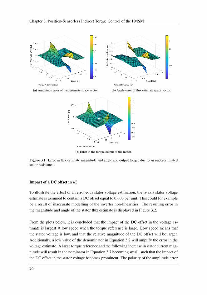
To demonstrate the impact of an erroneously estimated stator resistance, the resistance isassumed to be underestimated with 20%, such that rs = 0.8rs. This could correspond to ascenario in which the stator windings for some reason are experiencing high temperatures,such that the actual resistance is higher than the resistance that is given by the manufac-turer. This could be a result of high ambient temperatures, loading or frequency.
Figure 3.1 shows the error in the magnitude and angle of the flux estimate due to theunderestimated stator resistance during steady-state. Two important observations can bemade: The error in the flux estimate due to an erroneous rs increases with the magnitudeof the load torque and it also increases as the speed approaches zero. This can be under-stood by considering Equation 3.7. A large torque reference means that the stator currentmagnitude becomes large, and erroneous stator resistance will as such have a larger im-pact on the flux estimate, since the current and resistance are multiplied. The polarity ofthe magnitude error depends on whether the machine operates as generator or motor. Inmotor operation, the error between the real flux and the flux estimate is negative. Thisis because the stator voltage and the stator current will have the same polarity, and theunderestimated resistance will hence lead to the flux magnitude being estimated too large.Similarly, when the machine operates as a generator and the voltage and current have dif-ferent polarities, the underestimated resistance will result in a flux estimate that is smallerthan its real value, leading to a positive flux estimate error. When the speed is low, thestator voltage magnitude is small and the relative importance of the stator resistance in theflux estimate is larger. Additionally, the denominator in Equation 3.7 will then also besmall, and the impact of the inaccurate resistance estimate will be amplified.
An underestimated resistance rs = 0.8rs is seen to produce a steady-state amplitude errorof around 0.03 per unit and an angle error in excess of 1 degree. This results in an errorin the torque output of the machine that approaches 0.05 per unit when the torque refer-ence becomes large and the speed becomes low. The torque error is positive for negativespeeds, meaning that the actual motor torque is less than in the ideal case. For positivespeeds, the error is negative, which means that the motor will output a greater torque thanwhat it would if the resistance was accurately estimated.
25
Chapter 3. Position-Sensorless Indirect Torque Control of the PMSM
(a) Amplitude error of flux estimate space vector. (b) Angle error of flux estimate space vector.
(c) Error in the torque output of the motor.
Figure 3.1: Error in flux estimate magnitude and angle and output torque due to an underestimatedstator resistance.
Impact of a DC offset in uss
To illustrate the effect of an erroneous stator voltage estimation, the α-axis stator voltageestimate is assumed to contain a DC offset equal to 0.005 per unit. This could for examplebe a result of inaccurate modelling of the inverter non-linearities. The resulting error inthe magnitude and angle of the stator flux estimate is displayed in Figure 3.2.
From the plots below, it is concluded that the impact of the DC offset in the voltage es-timate is largest at low speed when the torque reference is large. Low speed means thatthe stator voltage is low, and that the relative magnitude of the DC offset will be larger.Additionally, a low value of the denominator in Equation 3.2 will amplify the error in thevoltage estimate. A large torque reference and the following increase in stator current mag-nitude will result in the nominator in Equation 3.7 becoming small, such that the impact ofthe DC offset in the stator voltage becomes prominent. The polarity of the amplitude error
26

3.1 Stator Flux Linkage Estimation
is dependent on whether the machine operates as a motor or a generator. During motoroperation, the DC offset will lead to the flux being estimated too small, such that the fluxestimate magnitude error becomes positive. Similarly, during generator operation, the DCoffset makes the flux estimate magnitude become larger than the real flux, such that theestimate error becomes negative. The voltage model seems to be highly sensitive to evensmall offsets in the stator voltage. In this case, a maximum amplitude error of around 0.1
per unit and a angle error of about 8 degrees is observed. The maximum torque error oc-curs during low-speed and high-torque operation, and the error magnitude appears to be inthe range of 0.05 per unit. The torque error is negative for negative speeds, which meansthat the torque output of the machine becomes greater than what it would be in the case ofa perfectly estimated stator voltage. For positive speeds, the voltage estimate error resultsin a reduction of the motor torque output, and the torque error becomes positive.
(a) Amplitude error of flux estimate space vector. (b) Angle error of flux estimate space vector.
(c) Error in the torque output of the motor.
Figure 3.2: Error in flux estimate magnitude and angle and output torque due to a DC offset in thestator voltage estimate.
27

Chapter 3. Position-Sensorless Indirect Torque Control of the PMSM
3.2 Rotor Position and Speed Estimation
The operation of the sensorless motor drive is divided into two main categories: Findinginitial position and ”operation enabled”. During the former, the initial position of the rotoris obtained and the stator flux estimate is initialized using the current model. In the latter,the rotor position is estimated in real time using the flux estimate from the voltage model.
3.2.1 The Initialization Procedure
In this project, freedom is given to rotate the rotor into a known initial position before themotor is started. This will be done by applying a DC current in the a-axis of the motorduring an initialization period of 3 seconds. During this period, the interaction betweenthe flux from the stator windings and the permanent magnet flux linkage will cause themagnetic axis of the rotor (i.e. the d-axis) to align with the a-axis of the stator. It shouldbe noted that this method is not an acceptable option in all cases, as the direction of mo-tion of the rotor will be unpredictable, which may have detrimental consequences in someapplications.
Once the initialization procedure is performed, the rotor angle will be 0 degrees and thecurrent model can be used to obtain the initial value of the stator flux estimate, ψs
s0. The
initial value produced by the current model is passed to the voltage model when the motoris started.
3.2.2 Operation Enabled: The Active Flux Concept
Once the initialization routine is completed, the motor drive enters the ”operation enabled”state. Here, the drive will rely on the voltage model flux estimate for position estimation.Once the stator flux linkage is estimated, an estimate for the rotor position and speed canbe obtained by introducing the active flux concept that transforms all salient-pole machinesinto fictitious, non-salient machines [40, 8, 7]. The active, or torque-producing, flux vec-tor is the flux that multiplies the q-axis current in the rotor-oriented torque expression inEquation 2.22. The active flux vector in the rotor-oriented reference frame, Ψr
T , is givenby
ψrT
= ψrm
+ (xd − xq)id (3.8)
Equation 3.8 can be further modified, and it can be shown that an expression for the activeflux vector that is valid in any reference frame is given by
ψT
= ψs− xqis (3.9)
28

3.2 Rotor Position and Speed Estimation
When the estimate for the stator flux linkage is found, an estimate for the active flux vectorcan be obtained by using Equation 3.9. From Equation 3.8, it is concluded that ΨT pointsin the same direction as the permanent magnet flux linkage and hence the rotor. The angleof ΨT with respect to the phase a axis thus corresponds to the angle of the rotor. This iscan be visualized by considering Figure 3.3.
Figure 3.3: The active flux space vector. Reproduced from [40].
An estimate for the active flux vector in stator coordinates, ψs
T, can be obtained using the
voltage model flux estimate, ψs
s,u, as shown in Equation 3.10.
ψs
T= ψ
s
s,u− xqiss (3.10)
The angle of ψT
sis equal to the rotor angle position, θ, and can be calculated by using the
inverse tangent function, as shown in Equation 3.11.
θ[k] = arctan
(ψT,β [k]
ψT,α[k]
)(3.11)
Here, ψT,α and ψT,β are the α and β components of the active flux vector, respectively.Once an estimate for θ is obtained, an approximate value for the per unit rotor speed canbe found as the time derivative of the position estimate as shown in Equation 3.12.
n[k] =θ[k]− θ[k − 1]
Tsamp(3.12)
29
Chapter 3. Position-Sensorless Indirect Torque Control of the PMSM
An equivalent expression for the speed estimate is given by Equation 3.13 [40]. This is theexpression that will be used for speed estimation in this thesis.
n[k] =ψT,α[k − 1]ψT,β [k]− ψT,β [k − 1]ψT,α[k]
Tsamp(ψ2T,α[k] + ψ2
T,β [k])(3.13)
Without additional filtering, the speed estimate produced by the equation above may be-come very noisy, which may cause problems for the control system. A low-pass filter istherefore applied to the speed estimate in order to reduce the noise in the estimate, withthe filter time constant being set equal to 0.005 seconds. The time constant value is ob-tained through trial and error, and the chosen value was the smallest value that resulted inadequate filtering of the speed estimate. As low-pass filtering will introduce a delay be-tween the filtered speed estimate and the unfiltered estimate that increases for increasingfilter time constant magnitude, the time constant value should be kept as small as possible.In [8], a value of similar magnitude was deemed appropriate, and thus supports the filterdesign that is chosen in this thesis.
3.3 On-Line Stator Voltage Estimation
To achieve further reductions in drive hardware complexity, cost, size and weight, as wellas increased reliability, the stator voltage sensors can be removed, and the stator voltagecan be estimated on-line. Such an approach will be taken in this thesis, and is presented inthis section.
A common technique for stator voltage estimation is to use the reference voltages pro-vided by the controllers as a means of obtaining the output voltage of the inverter. Ideally,the inverter’s output voltage would be identical to the reference voltage of the converter. Inreality, however, the non-ideal properties of the inverter will lead to discrepancies betweenthe reference voltage and the actual stator voltage, as non-linear voltage drops across theconverter produces distortion in its output voltage. Especially during low speed operationwhen the stator voltage is low, the voltage might become highly distorted.
If the non-linear voltage drops across the inverter are accurately modelled, they can besubtracted from the reference voltage in order to compensate for the voltage drop acrossthe inverter and achieve a realistic estimate of the output voltage. This will make it pos-sible to operate the motor drive without using voltage sensors. In the following sections,this approach is described. A thorough analysis of how on-line stator voltage estimationcan be performed was conducted by Fjellanger in his master’s thesis, and the interested
30
3.3 On-Line Stator Voltage Estimation
reader is referred to [16] for a more comprehensive discussion.
3.3.1 Non-Ideal Converters: Influence of Dead Time Effects
The three-phase, two-level converter that is used in the PMSM drive has three bridge legs,with each leg having two transistors and two free-wheeling diodes, as shown in Figure 3.4.Ideally, the transistors are switched such that when one of them is in its ON state, the otherone is off. In practice, there will be a short period of time, referred to as the blanking timeTBT , in which both transistors in a converter leg are off simultaneously [34]. This is doneto avoid ”shoot-through”, or short-circuiting of the converter leg, as the turn-on delay timeensures that the device is completely turned off and does not turn back on again when thecomplementary transistor is turned on. If shoot-through were to occur, it is likely that theswitches would be destroyed by the high short-circuit current.
Figure 3.4: Generic three-phase, two-level voltage source converter. Reproduced from [34].
In addition to the blanking time, there will be a delay between the time of the turn oncommand and the instant when the device actually starts conducting. When a gate pulseis applied to the switch, the voltage across it will start to rise and the switch does not startto conduct before a certain voltage is reached. The period of time it takes for the voltageto increase above its threshold value and start conducting is referred to as the turn-on timeof the transistor. Similarly, when the turn-off command is applied, there will be a periodof time when the voltage across the device decreases, and when the voltage drops belowa given value, the switch will stop conducting. This period of time is referred to as the
31

Chapter 3. Position-Sensorless Indirect Torque Control of the PMSM
transistor’s turn-off time. The turn-on and turn off-times of the transistor can generally beincorporated into the blanking time.
As described in the paragraph above, there will be a constant voltage drop across the tran-sistor, uPN , that is necessary for current to flow across the PN junction of the transistor.This also applies to the freewheeling diode. Additionally, both the transistor and the diodewill cause an ohmic voltage drop due to their internal resistances, rT . The combined ef-fects of blanking time, turn-on and turn-off time and the voltage drops across the switchesand diodes are usually referred to as the dead time effects of the converter. If these areaccurately modelled, the real stator voltage can be estimated with high precision.
3.3.2 Estimating the Stator Voltage
Analytical expressions for the approximate value of the voltage drop across the converteras a result of the dead time effects in the converter, ∆us,DT , were developed by Weichboldand von Raumer in [49] and are presented in Equation 3.14.
∆us,DT = sign(is)
(uTD(|is|) +
Td + Ton − ToffTs
· uDC)
(3.14)
Here, uTD is the averaged on-state voltage drop of transistor and diode, which is dependenton the current magnitude. TBT is the blanking-time of the transistor, while Ton and Toffare the the turn-on and turn-off time, respectively. If the on-state voltage drop across theconverter switches and diodes are neglected, a simple approximation of the voltage dropsacross the converter due to the dead-time effects is given by
∆us,DT = −sign(is)Td + Ton − Toff
Ts· uDC (3.15)
This is a reasonable approximation, since the magnitude of the DC link voltage is muchlarger than the on state voltage drop of the diode and transistor [16]. Once the value of∆uDT is obtained for each phase, the output stator voltage, uss can be estimated using
uss = uss,ref + ∆uss,DT (3.16)
where uss,ref represents the reference voltage to the converter.
As seen from the expressions above, the voltage drop across the semiconductors is de-pendent on the direction of the current flowing out of the converter. When the current ispositive, the value of ∆us,DT becomes negative, which leads to the output voltage becom-ing smaller than the reference voltage. When the current is negative, ∆us,DT becomes
32

3.4 Sensorless Operation Based on the Voltage Model
positive and the output voltage becomes larger than the reference voltage. In Figure 3.5,the reference voltage of the converter, which corresponds to the ideal stator voltage, andthe estimated output stator voltage, which is an approximation of the actual output voltageof the converter, are presented. The stator current is also included in the plot. Here, it hasbeen assumed that the combined turn-on, turn-off and blanking time amount to 10% of thesampling period. This is an unrealistically high value, but allows for easy visualization ofthe dead-time effects on the output voltage of the converter. In the figure it can be seenthat there is an instantaneous change in the output voltage when the current crosses thezero-line.
Figure 3.5: Ideal stator voltage, estimated stator voltage and stator current of phase a of the motor.
3.4 Sensorless Operation Based on the Voltage Model
In Section 3.1, the voltage model and the current model were presented, and it was shownhow they can be used to estimate the stator flux linkage of the motor. Once a flux estimateis obtained, the rotor position of the machine can be estimated using the active flux conceptthat was presented in Section 3.2. Since the current model estimates the flux in the dqplane, it alone cannot be used for flux estimation in a position-sensorless motor drive, and
33
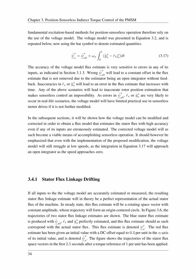
Chapter 3. Position-Sensorless Indirect Torque Control of the PMSM
fundamental excitation-based methods for position-sensorless operation therefore rely onthe use of the voltage model. The voltage model was presented in Equation 3.2, and isrepeated below, now using the hat symbol to denote estimated quantities.
ψs
s= ψ
s
s0+ ωn
∫ t
0
(uss − rsiss)dt (3.17)
The accuracy of the voltage model flux estimate is very sensitive to errors in any of itsinputs, as indicated in Section 3.1.3. Wrong ψ
s
s0will lead to a constant offset in the flux
estimate that is not removed due to the estimator being an open integrator without feed-back. Inaccuracies in rs or uss will lead to an error in the flux estimate that increases withtime. Any of the above scenarios will lead to inaccurate rotor position estimation thatmakes sensorless control an impossibility. As errors in ψ
s
s0, rs or uss are very likely to
occur in real-life scenarios, the voltage model will have limited practical use in sensorlessmotor drives if it is not further modified.
In the subsequent sections, it will be shown how the voltage model can be modified andcorrected in order to obtain a flux model that estimates the stator flux with high accuracyeven if any of its inputs are erroneously estimated. The corrected voltage model will assuch become a viable means of accomplishing sensorless operation. It should however beemphasized that even with the implementation of the proposed modification, the voltagemodel will still struggle at low speeds, as the integration in Equation 3.17 will approachan open integrator as the speed approaches zero.
3.4.1 Stator Flux Linkage Drifting
If all inputs to the the voltage model are accurately estimated or measured, the resultingstator flux linkage estimate will in theory be a perfect representation of the actual statorflux of the machine. In steady state, this flux estimate will be a rotating space vector withconstant amplitude, whose trajectory will form an origin-centered circle. In Figure 3.6, thetrajectories of two stator flux linkage estimates are shown. The blue stator flux estimateis produced with ψ
s0, rs and uss perfectly estimated, and this flux estimate should as such
correspond with the actual stator flux. This flux estimate is denoted ψss. The red flux
estimate has been given an initial value with a DC offset equal to 0.3 per unit in the α-axisof its initial value, and is denoted ψ
s
s. The figure shows the trajectories of the stator flux
space vectors in the first 2.5 seconds after a torque reference of 1 per unit has been applied.
34

3.4 Sensorless Operation Based on the Voltage Model
Figure 3.6: Real stator flux and flux estimate trajectories with erroneous initialization of the voltagemodel.
In Figure 3.6, it appears that the stator flux estimate has ”drifted” away from the origin andbecome non-origin centered due to the erroneous initialization of the flux vector, demon-strating how the flux estimate vector may behave if it is erroneously estimated with thevoltage model. In Figure 3.7, the time-series of the magnitudes and angles of the esti-mated and the real flux, as well as the magnitude error and the angle error of the fluxestimate, are presented for the same scenario. The magnitude and angle error of the fluxestimate are calculated as |ψs
s| − |ψ
s
s| and ∠ψs
s− ∠ψ
s
s, respectively. Here, it can be seen
that when the flux estimate drifts, the result is oscillating errors in both the magnitude andthe angle of the flux estimate. This can be understood by considering Figure 3.6. When ψ
s
s
is pointing in the positive α-axis direction, its magnitude is larger than that of ψss, while
it becomes smaller after half electric period when the space vector has rotated 180. It isworth mentioning that the magnitude of ψ
s
sin theory should be constant, given that it is
estimated with no errors added to ψs0
, rs or uss, but a small oscillation in the real statorflux’ magnitude is observed as well in Figure 3.7a. This is most likely due to inherentinaccuracies in the current and voltage readings in the embedded real-time simulator, e.g.round-off errors, which results in some drifting of ψs
sas well.
35

Chapter 3. Position-Sensorless Indirect Torque Control of the PMSM
(a) Magnitude of the stator flux estimates. (b) Angle of the stator flux estimates.
(c) Flux estimate magnitude error. (d) Flux estimate angle error.
Figure 3.7: Voltage model flux estimate with erroneous initialization and voltage model flux esti-mate with all quantities accurately estimated.
Similar drifting of the flux estimate can be observed if there are offsets in the estimatedstator voltage or if the stator resistance is erroneously estimated. These two scenariosare presented in Figure 3.8, where the blue and red flux estimates once again representthe accurate flux estimate and the erroneous flux estimate, respectively. In Figure 3.8athe stator voltage estimate contains a DC offset equal to 0.005 per unit in the α-axis,while in Figure 3.8b, the resistance is assumed to be underestimated with 20%, such thatrs = 0.8rs. While an erroneous flux initial value will remain in the flux estimate as aconstant error, any errors in uss and rs will be integrated in the voltage model for each timestep, producing an flux estimate that drifts further and further away from the origin withtime. Such errors therefore present a more severe problem than erroneous initialization ofthe flux estimate.
36
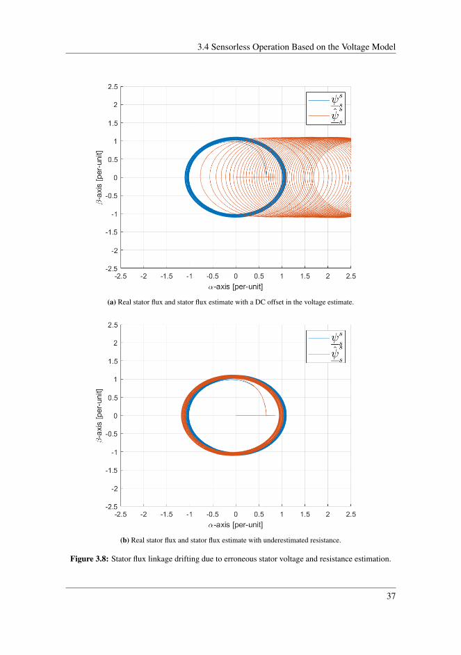
3.4 Sensorless Operation Based on the Voltage Model
(a) Real stator flux and stator flux estimate with a DC offset in the voltage estimate.
(b) Real stator flux and stator flux estimate with underestimated resistance.
Figure 3.8: Stator flux linkage drifting due to erroneous stator voltage and resistance estimation.
37

Chapter 3. Position-Sensorless Indirect Torque Control of the PMSM
3.4.2 Stator Flux Linkage Drift Correction: The Niemela Method
To ensure that the flux estimate remains sufficiently accurate for the drive to operate with-out a position sensor, methods that prevent drifting due to errors in the inputs to the voltagemodel must be implemented.
Several methods for compensation of the drifting phenomenon have been proposed overthe years. Wu and Slemon presented in [50] a method for drift compensation in which theextreme points of the flux estimate locus in the complex plane are used to generate sepa-rate correction terms for the real and imaginary components of the flux estimate. Anothercommon approach to dealing with the drift problem is replacing the open integrator with alow-pass filter. However, the low-pass filter introduces an error in the phase angle and themagnitude of the flux estimate. Hu and Wu suggested in [27] three methods for modifyingthe low-pass filter by adding feedback compensation signals in order to reduce the fluxestimate errors the low-pass filter causes.
Niemela presented in [36] an alternative method for generating flux estimate correctionterms that relies on the estimated flux vector itself, which will be adopted in this thesis.This method was shown to be capable of correcting flux drift for frequencies above 0.5 Hzin a 50 Hz synchronous machine, and even worked sufficiently for frequencies as low as0.1 Hz. In the Niemela method, the magnitude of the erroneous flux estimate is squaredand filtered using a low-pass filter, and the difference between the filtered, squared estimateand the squared estimate is used to obtain an error, ε. That is,
ε = |ψs
s|2filtered − |ψ
s
s|2 (3.18)
The error, ε, is multiplied with an correction coefficient, kψ,corr, and added to the originalflux estimate, such that the after-correction estimate, ψ
s
s[k], becomes
ψs
s[k] = (1 + kψ,corr[k] · ε[k]) · ψ
s
s[k] = ψ
s
s+ ψs
s,corr(3.19)
The drift-compensated flux estimate can hence be considered the sum of the original fluxestimate and a correction component.
The low-pass filter that is used has the transfer function
HLPF (s) =1
1 + Tfs(3.20)
38

3.4 Sensorless Operation Based on the Voltage Model
where Tf is the filter time constant. The filtering process of |ψs
s|2, can hence be written as
|ψs
s|2filtered(s) =
1
1 + Tfs|ψs
s|2(s) (3.21)
which in discrete-time can be expressed as
|ψs
s|2filtered[k + 1] = |ψ
s
s|2filtered[k] +
TsampTf
(|ψs
s|2[k]− |ψ
s
s|2filtered[k]) (3.22)
The validity of the Niemela drift correction concept can be demonstrated by consideringFigure 3.9. Here, the flux estimate drifts due to an underestimated resistance, rs = 0.8rs.When the flux estimate drifts, the square of the magnitude of the flux will oscillate aroundits filtered value and produce a time-varying error signal. The error signal that is gen-erated carries information about the instantaneous magnitude and direction of the drift:From Figure 3.9 it can be seen that when the error signal is positive, the square of the fluxmagnitude is smaller than the filtered value, meaning that positive correction flux mustbe added to produce the after-correction estimate. The magnitude of the correction com-ponent is proportional to the magnitude of ε, such that if the magnitude of ε is large, themagnitude of ψs
s,corrwill increase. Similarly, a negative ε indicates that a negative correc-
tion flux should be added to produce the after-correction estimate, with the magnitude ofthe correction being proportional to the magnitude of ε.
39

Chapter 3. Position-Sensorless Indirect Torque Control of the PMSM
Figure 3.9: Flux estimate magnitude squared, flux estimate magnitude squared and filtered and theerror signal.
The speed of rotation of the flux estimate space-vector will be equal to the frequency ofthe stator currents, meaning that the frequency of the drift-induced ripple in the squaredflux estimate also will be equal to the stator frequency. To achieve effective filtering of theripple in the flux estimate due to drifting, the time constant of the low-pass filter shouldtherefore be made a function of the stator frequency. At low frequencies, the frequencyof the ripple in |ψ
s
s|2 is low, meaning that a large filter time constant will be necessary.
Similarly, when the stator frequency is large, the frequency of the ripple in the |ψs
s|2 will
be large, and a smaller filter time constant is then sufficient to filter it out. To ensure that
40

3.4 Sensorless Operation Based on the Voltage Model
the filter time constant is adequately larger than the electric time period of the drift-inducedripple, the following formula will be used to obtain the filter time constant:
Tf =2
n · fn(3.23)
Here, n and fn are the estimated motor speed and the nominal frequency, respectively.This formula yields a filter time constant that is approximately twice the electric period.Looking at the suggested formula, however, it is apparent that its value will grow very largeduring low operating speeds. When the time constant becomes very large, any variations inthe stator flux linkage estimate due to changes in the torque reference could be eliminatedby the filter, resulting in an inaccurate flux estimate. To avoid this, the time constant willbe limited to a maximum value of 1.75, as proposed by [17]. The final formula for thefilter time constant then becomes
Tf = min
(2
n · fn, 1.75
)(3.24)
In Figure 3.10, the torque reference, the estimated speed and the value of the low-passfilter time constant during start-up of the motor are shown. During the initial moments ofthe start-up transient when the estimated speed is low, the filter time constant exceeds, andis therefore limited to, its maximum limit of 1.75. As the speed increases, the value of thefilter time constant decreases until it reaches its steady-state value of approximately 0.04
seconds. This is twice the electric time period of the nominal frequency of 50 Hz.
(a) Torque reference and estimated speed. (b) Low-pass filter time constant.
Figure 3.10: Low-pass filter time constant during start-up.
41

Chapter 3. Position-Sensorless Indirect Torque Control of the PMSM
3.4.3 Modifying the Low-Pass Filter
As discussed by Luukko in [32], the dynamic behaviour of the low-pass filter that wasproposed by Niemela is not sufficient during rapid torque transients. During a step in thetorque reference, the real stator flux squared will change as a result of the stator currentsresponding to a change in the reference values that are passed to the control system. Thefiltered square of the flux that is employed in the Niemela method will however changeconsiderably slower than the non-filtered value, which leads to the error vector, and hencethe drift correction term, becoming non-zero. As a result, the flux estimate will be cor-rected during the torque transient, preventing the flux estimate from following the actualflux.
In Figure 3.11, this concept is demonstrated. Here, the response in (ψs
s)2 and (ψ
s
s)2filtered
to a step in the torque reference can be seen. All inputs to the voltage model are assumedto be perfectly measured, which means that the flux estimate will not drift and correctionof the estimate should as such not be necessary. The machine is at a standstill when thetorque reference step is applied, meaning that the time constant of the low-pass filter islarge. The filtered square of the flux therefore responds considerably slower to the torquereference step than the non-filtered value, creating a difference between the two that leadsto a non-zero ε. As a result, the change in flux during the torque reference transient isrecognized as drifting that needs correction, and an undesirable correction flux componentψss,corr
is generated. The α and β components of the correction flux is shown in the bottomplot in Figure 3.11.
42

3.4 Sensorless Operation Based on the Voltage Model
(a) Torque reference.
(b) Flux estimate magnitude squared and flux estimatemagnitude squared and filtered.
(c) α and β components of the correction flux.
Figure 3.11: Dynamics of the squared flux estimate, the squared and filtered flux estimate and thecorrection flux during a torque reference transient.
43

Chapter 3. Position-Sensorless Indirect Torque Control of the PMSM
In [32], Luukko proposed to modify the low-pass filter that is used to filter the square of theflux estimate to avoid drift correction during rapid torque reference transients. If the filteracts as a unity gain during the transient, the error vector is forced to zero and no correctionis done. This is done by adding a derivative term to the previously used low-pass filter,such that it can be written as
HLPF (s) =1 + Td · s1 + Tf · s
(3.25)
The relationship between the input and the filtered output of the filter in discrete time isnow given by
|ψs
s|2filtered[k + 1] = |ψ
s
s|2filtered[k] +
TsampTf
(|ψs
s|2[k]− |ψ
s
s|2filtered[k])+
TdTf
(|ψs
s|2[k]− |ψ
s
s|2[k − 1]) (3.26)
whereTdTf
= kT (3.27)
From Equation 3.25, it is seen that if kT is equal to 1, the modified low-pass filter becomesa unity gain and no drift correction is performed. If kT is equal to 0 on the other hand, thederivative term in the modified low-pass filter is eliminated and correction is performed.The value of kT will be calculated based on Equation 3.28:
kT = min (1, kT0|τe − τe,filtered|) (3.28)
Here, τe is the estimated value of the electromagnetic torque, which is found using Equa-tion 2.20. The d and q axis currents in the torque equation are obtained using the estimatedrotor position from the voltage model. τe,filtered is a low-pass filtered value of the torqueestimate, that is obtained using a low-pass filter with a filter time constant equal to 0.1
seconds, and the difference between τe and τe,filtered will be approximately equal to theper unit value of the torque step when it occurs. The value of the coefficient kT0 can beused to modify the behaviour of kT : E.g., to disable drift correction for torque steps equalto or larger than 0.5 pu, kT0 should be equal to 2. The correction coefficient kψ,corr canthen be forced to zero during torque reference steps by defining
kψ,corr = (1− kT )kψ0 (3.29)
According to [38], a typical value of kψ0 is 0.0075, and this is the value that will be usedhere.
44
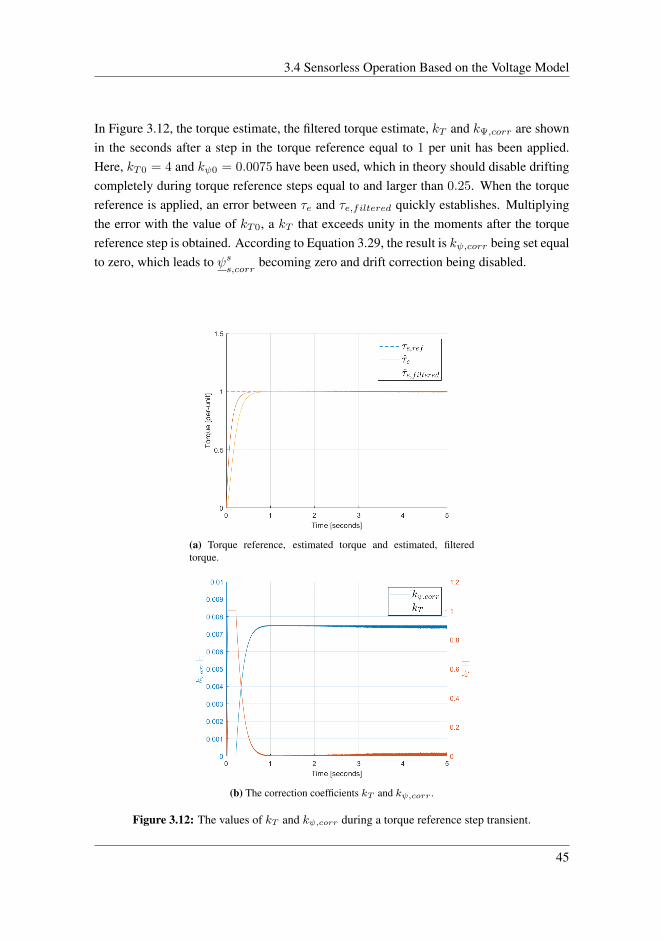
3.4 Sensorless Operation Based on the Voltage Model
In Figure 3.12, the torque estimate, the filtered torque estimate, kT and kΨ,corr are shownin the seconds after a step in the torque reference equal to 1 per unit has been applied.Here, kT0 = 4 and kψ0 = 0.0075 have been used, which in theory should disable driftingcompletely during torque reference steps equal to and larger than 0.25. When the torquereference is applied, an error between τe and τe,filtered quickly establishes. Multiplyingthe error with the value of kT0, a kT that exceeds unity in the moments after the torquereference step is obtained. According to Equation 3.29, the result is kψ,corr being set equalto zero, which leads to ψs
s,corrbecoming zero and drift correction being disabled.
(a) Torque reference, estimated torque and estimated, filteredtorque.
(b) The correction coefficients kT and kψ,corr .
Figure 3.12: The values of kT and kψ,corr during a torque reference step transient.
45

Chapter 3. Position-Sensorless Indirect Torque Control of the PMSM
With the Niemela-method for drift correction and the modified low-pass filter for driftdisabling during torque reference steps properly implemented, the corrected voltage modelshould be able to provide accurate flux estimation even in the presence of inaccuracies inψs
s0, rs or uss. Sensorless operation based on the Niemela-corrected voltage model will be
investigated in Chapter 4.
3.5 Sensorless Operation Based on the Voltage-CurrentModel
In the previous section, the Niemela-corrected voltage model was presented as a means ofobtaining accurate flux estimation in scenarios where the uncorrected voltage model willfail. In this section, a closed-loop flux observer that combines both the voltage model andthe current model for flux estimation is presented as an alternative method for flux estima-tion during sensorless operation.
As discussed in the previous section, the voltage model provides inaccurate flux estimateswhen the stator frequency is low, and it relies on some sort of drift compensation to correctfor inaccurate model inputs. The current model, on the other hand, is accurate across thewhole speed range if the model parameters are accurate and the rotor position is known.Bauer and Heining and Jansen and Lorenz suggested in [4] and [25], respectively, to com-bine the voltage and the current models with the goal of obtaining an improved flux model.In the proposed solution, the flux estimate from the current model acts as a reference valuefor the flux estimate from the voltage model to follow. The error between the two fluxestimates is fed back to the voltage model via a controller, usually a proportional or a pro-portional plus integral controller, and hence acts as a stabilizing feedback term. The errorbetween the reference flux and the output flux, εs, is then given by
εs = ψs
s,i− ψ
s
s,u(3.30)
This error signal is passed to the controller in the feedback loop, which outputs a compen-sation voltage, uss,comp, that is added to voltage model integral. The flux estimate from thevoltage model now becomes
ψs
s= ψ
s
s0+ ωn
∫ t
0
(uss − rsiss + uss,comp)dt (3.31)
46

3.5 Sensorless Operation Based on the Voltage-Current Model
Separately, the voltage model and the current model are open-loop estimators, but by com-bining them as suggested, a closed-loop observer is obtained [25]. The structure of thevoltage-current model is presented in Figure 3.13. Here, a proportional controller is usedin the feedback-loop and the active flux concept is utilized for rotor position and speedestimation.
Figure 3.13: The voltage-current model with a proportional controller in the feedback loop. Repro-duced from [33].
The closed-loop observer combines the advantages of the current model during low-speedoperation with those of the voltage model during medium-high speed operation to providean improved flux estimate. In general, the current model in the closed-loop observer canuse the estimated or measured rotor position in order to transform stator-frame quantitiesinto rotor-oriented quantities. For sensorless control applications, such as the one that iscurrently being considered, the input to the current model will be the estimated rotor anglefrom the voltage model. As a result, the closed-loop observer will still struggle duringoperation around zero speed.
3.5.1 Using a Proportional Controller in the Feedback Loop
In the method presented in [4], a proportional controller with a gain of kp was used inthe feedback loop in order to determine for which frequency the observer would transitionfrom being current model reliant, to becoming reliant on the voltage model. The signifi-cance of the value of the feedback gain can be shown mathematically by considering theclosed-loop transfer function from the current model reference flux estimate, ψ
s
s,i, to the
47

Chapter 3. Position-Sensorless Indirect Torque Control of the PMSM
voltage model output flux estimate, ψs
s,u. The stator voltage, uss, and the product of the
stator resistance and the stator current, rsiss, that are inputs to the voltage model can beconsidered disturbances that act on the control loop that is the closed-loop observer. Usingthe principle of superposition, these can be set equal to zero, and the impact of ψ
s
s,ion
ψs
s,ucan be investigated. The transfer function from the reference flux to the output flux
becomesψs
s,u
ψs
s,i
=kp
s+ kp(3.32)
For small frequencies s kp, the transfer function magnitude approaches unity, indi-cating that the flux estimate from the closed-loop observer follows the current model es-timate closely in the low-speed region. When s kp, the transfer function magnitudeapproaches zero, which means that the flux estimate is now given by the voltage model.When s = kp, the magnitude of the transfer function becomes 1
2 , meaning that the voltagemodel and the current model are trusted equally when producing the output flux estimate.Hence, by choosing the value of kp, the speed for when the closed-loop observer transi-tions from being current-model reliant to becoming voltage-model reliant can be set.
The impact of the disturbances, uss and rsiss, on the flux estimate can be exemplified byconsidering the transfer function from the stator voltage estimate uss to the voltage modelflux estimate, ψ
s
s,u. As before, using the principle of superposition, the effect of the volt-
age on the voltage model flux estimate can be found by setting the current model fluxestimate, ψ
s
s,i, equal to zero. The following transfer function is obtained:
ψs
s,u
uss=
1
s+ kp(3.33)
The effect of a DC offset in uss equal to ∆uss can be found using the final value theorem asshown below:
limt→∞
ψs
s,u(t) = lim
s→0s
(1
s+ kp
)∆usss
= ∆uss (3.34)
This shows that potential DC offsets in uss and rsiss will remain drift-inducing sourcesof error in the flux estimate that will not be removed over time. This can be verifiedby considering Figure 3.14. Here, a DC offset equal to 0.005 per unit is present in theα-axis stator voltage, and the response in the α-axis stator flux estimate is shown. Theproportional controller is tuned with kp = 0.1. From the figure, it is evident that theamplitude of the response in the α-axis flux estimate to the DC offset has a steady-statevalue equal to 0.05 per unit.
48

3.5 Sensorless Operation Based on the Voltage-Current Model
Figure 3.14: Response in the α-axis flux magnitude from the proportional controller based voltage-current model to a DC offset in the stator voltage.
49
Chapter 3. Position-Sensorless Indirect Torque Control of the PMSM
3.5.2 Using a Proportional-Integral Controller in the Feedback Loop
To eliminate the steady-state error in the flux estimate due to errors in the inputs to thevoltage model that were observed in the previous section, integral effect can be added tothe controller in the observer’s feedback loop. The combination of the PI-controller basedvoltage-current model and the active flux concept for rotor position and speed extractionin PMSM drives has been investigated in [40, 41, 8, 7, 8, 44]. The structure of this config-uration is presented in Figure 3.15. The only difference compared to the voltage-currentmodel from the previous section is that a PI controller is now used in the feedback loop.
Figure 3.15: The voltage-current model with a proportional-integral controller in the feedback loop.
The PI controller transfer function can be written as
HPI(s) = kp +kis
(3.35)
where kp and ki are the proportional and the integral gains of the controller, respectively.When replacing the proportional controller in the feedback loop of the voltage-currentmodel with a PI controller, the closed-loop transfer function becomes
ψs
s,u
ψs
s,i
=ψsψsi
=kps+ ki
s2 + kps+ ki(3.36)
50

3.5 Sensorless Operation Based on the Voltage-Current Model
while the transfer function from the stator voltage estimate to the flux estimate becomes
ψs
s,u
uss=
s
s2 + kps+ ki(3.37)
As before, the effect of a DC offset in the estimated stator voltage on the flux estimate canbe investigated using the final value theorem:
limt→∞
ψs
s,u(t) = lim
s→0s
(s
s2 + kps+ ki
)∆usss
= 0 (3.38)
Equation 3.38 shows that by adding integral effect to the controller in the feedback loop,the controller will eliminate the effect of errors in the input to the voltage model that wouldotherwise cause drifting of the flux estimate. Figure 3.16 shows the response of the α-axisflux estimate to a DC offset in the α-axis of the stator voltage estimate equal to 0.005per unit with the PI controller implemented in the feedback loop. The controller has beentuned using kp = 0.1 and ki = 0.1. From the plot it is evident that by adding integral effectto the feedback controller, the impact of the DC offset in the estimated stator voltage onthe α-axis flux estimate magnitude is eliminated over time.
Figure 3.16: Response in the α-axis flux magnitude from the proportional-integral controller basedvoltage-current model to a DC offset in the stator voltage.
When proportional control was applied in the feedback loop, the relative importance ofthe voltage model and the current model in the closed-loop observer could be determined
51

Chapter 3. Position-Sensorless Indirect Torque Control of the PMSM
simply by choosing the value of the proportional gain of the controller. When using a PIcontroller, choosing appropriate values of the controller gains becomes a bit more com-plex, and the tuning process usually involves a degree of trial and error. An educatedguess of the controller gains can however be made using the pole placement method that isdescribed next. The closed-loop observer’s characteristic equation is given by the denom-inator polynomial of the closed-loop transfer function in Equation 3.36. This equation canalso be expressed as a function of the system poles, λ1 and λ2, with λ1 ≤ λ2, yielding thefollowing relationship:
s2 + kps+ ki = (s− λ1)(s− λ2) (3.39)
The PI controller gains can hence be written as a function of the closed-loop observerpoles, as shown in Equation 3.40.
kp = −(λ1 + λ2) (3.40a)
ki = λ1λ2 (3.40b)
As described in [2], the system poles will characterize the observer’s frequency behaviourin the following manner: The current model prevails for low frequencies when s < |λ1|,while the voltage model will prevail for s > |λ1|. A smooth transition between the twowill take place for |λ1| < s < |λ2|. The method of pole placement can provide a startingpoint for the tuning of the PI controller, but in practice, trial and error will be necessary toobtain PI controller gains that results in an accurate stator flux estimate. In this thesis, thePI controller will be tuned using kp = 0.1 and ki = 0.1. These values produce an accuratestator flux estimate, and will be used in the remainder of this thesis.
The voltage-current model with a PI controller in the feedback loop is the configurationthat will be used for the remainder of this thesis.
3.6 Possible Improvements of the Sensorless Control Schemes
This section contains a brief description of two concepts that can be used to improve theperformance of the sensorless motor drive. Both concepts were attempted in this thesis,but not successfully implemented, and remain strong candidates for future work that canserve to boost the performance of the sensorless control schemes that have been proposed.
52

3.6 Possible Improvements of the Sensorless Control Schemes
3.6.1 Phase-Locked Loop for Rotor Position Estimate Filtering
The inverse tangent function that is used in Equation 3.11 to extract the rotor positionfrom the active flux vector might produce a noisy position estimate if there is significantamount of harmonics present in the active flux vector estimate [20]. The differentiationof the position to obtain the speed estimate may as a consequence become very pollutedwith noise. Especially when driving through zero speed, this effect may become prevalentas a consequence of inaccurate flux vector estimates from the voltage model around zero-speed. To diminish the potential noise in the position and speed estimate, a phase-lockedloop (PLL) can be used to filter the estimated rotor position, as suggested in [38]. Thisapproach was investigated by Bolstad in [9], and resulted in increased accuracy of theclosed-loop observer, assuming erroneous stator resistance values. A description of thephase-locked loop, the proposed method and the results that were obtained are presentedin Appendix F.
3.6.2 High Frequency Signal Injection for Standstill and Low-SpeedOperation
In order to provide a comparison of the proposed fundamental-excitation based methodsand saliency-tracking based methods for sensorless operation during low-speed operation,attempts were made to implement the high-frequency signal-injection method for saliencytracking that is presented in [44]. This method is based on the work done by [52] and[28], and works by adding a square-wave voltage component with small amplitude andfrequency equal to the switching frequency to the d-axis stator voltage. The ripple in thestator current due to the high-frequency component in the stator voltage will be modulatedwith information about the rotor position, and by applying the correct demodulation tech-nique, the position of the rotor can be obtained [28]. In the proposed method, an attemptto extract the rotor position using a phase-locked loop was made, but it was not successful.A more detailed description of the approach can be found in Appendix G.
53

Chapter 3. Position-Sensorless Indirect Torque Control of the PMSM
54
Chapter 4Real-Time Simulation Results
In this chapter, the sensorless control schemes that were presented in the previous chapterwill be validated through simulation. The C++ sub-routines that are necessary for sen-sorless operation are added to existing control software in the programmable CPU of theSoC-based embedded controller that was presented in Section 2.3. Condensed versions ofthe most essential sub-routines are presented in Appendix H. These include subroutinesfor rotor position estimation using the active flux concept, stator voltage estimation andflux estimation using the Niemela-corrected voltage model and the voltage-current modelwith a PI controller in the feedback loop.
The control software will in this chapter be used to drive the ERTS that runs on the FPGAof the SoC. The data for the motor drive that is implemented in the ERTS are presented inAppendix B.
Two methods for flux estimation that in combination with the active flux concept enablesensorless operation were presented in the previous chapter, and will be simulated in thischapter. They are:
1. Sensorless operation based on the Niemela-corrected voltage model.
2. Sensorless operation based on the voltage-current model with a PI controller in thefeedback loop. This flux model will be referred to as the ”voltage-current model” inthe remainder of this thesis.
55

Chapter 4. Real-Time Simulation Results
The Load
Initially, all simulations will be performed using a quadratic load function that is dependenton the rotor speed. The load torque will be given by
τL = kn2 (4.1)
where the constant k is chosen such that the motor operates at nominal power at nominalspeed. This load characteristic is valid for the modelling of fans, pumps and compressors[37].
Resistance and Voltage Estimation
To verify the validity of the sensorless control algorithms, the stator resistance will beassumed erroneously estimated in order to create scenarios in which the flux estimatewill drift unless the proposed flux models work as intended. The stator resistance will beestimated such that
rs = 0.8rs (4.2)
According to Bolstad, this scenario will occur at 91C for copper-based stator windings ifthe value of rs is accurately estimated at 25C and then treated as a constant [9]. It may assuch correspond to a situation in which the machine is heavily loaded, subjected to highambient temperatures or both.
The stator voltage will be estimated according to the method presented in Section 3.3in all simulations, and the drift correction algorithms will therefore have to correct driftingthat results from both the inaccuracy in the resistance estimate and potential inaccuraciesin the voltage estimate. All other motor parameters are assumed to be accurate.
Simulation Cases
The following cases will be simulated:
1. Sensorless operation without correction
2. Sensorless operation based on the Niemela-corrected voltage model
(a) High-Speed Operation Including Start-Up
(b) Driving Through Zero-Speed
(c) Very-Low Speed Operation
56

4.1 Sensorless Operation Without Drift Correction
i. Start-Up and Very-Low Speed Operation
ii. Very-Low Speed Operation With High Initial Speed
(d) Driving Through Zero-Speed With Constant Load Torque
3. Sensorless operation based on the voltage-current model
(a) High-Speed Operation Including Start-Up
(b) Driving Through Zero-Speed
(c) Very-Low Speed Operation
i. Start-Up and Very-Low Speed Operation
ii. Very-Low Speed Operation With High Initial Speed
(d) Driving Through Zero-Speed With Constant Load Torque
4.1 Sensorless Operation Without Drift Correction
As an initial test, an attempt is made to operate the motor drive using the estimated statorflux from the voltage model without drift correction. This is done to demonstrate the needfor specialized flux models when the inputs to the voltage model are inaccurately mea-sured or estimated.
Figure 4.1 shows the true and estimated rotor position and the error between them in theseconds after a torque reference of 1 per unit is applied. The true speed, the estimatedspeed and the difference between them, along with the torque reference and the estimatedtorque, are also presented. The estimated torque is obtained using the torque expressionin Equation 2.20. With all machine reactances assumed to be accurately measured or esti-mated, the estimated torque is equal to the actual torque output of the motor.
From Figure 4.1 it can be seen that an error in the estimated rotor position is establishedimmediately after the torque reference is applied. During the initial start-up transient whenthe speed and the stator voltage is low, the flux estimate will be highly sensitive to the er-roneous stator resistance estimate. The result is oscillating errors in both flux estimate androtor position estimate. As the speed increases and approaches nominal speed, the impactof the inaccurate resistance becomes smaller and the magnitude of the position estimateerror decreases. However, when the drive approaches its steady-state speed, the errors dueto the inaccurate resistance will start to accumulate in the flux estimate, and the result isthat the magnitude of the position estimate error will become increasingly large. Afterapproximately 5.5 seconds, the inaccuracy in the rotor position estimate leads to drive
57

Chapter 4. Real-Time Simulation Results
malfunction due to over-currents.
From the above results it is evident that an erroneous resistance estimate and the subse-quent drifting of the flux estimate will quickly lead to an inaccurate rotor position estimate,which in turn causes problems for the control system. If the rotor position is inaccurate,the d- and q-axis current references will become erroneous and the performance of themotor drive will degrade. The following is thus clear: Flux models that are capable ofestimating the stator flux with high accuracy even when the stator resistance estimate iserroneous are necessary for sensorless operation of the motor drive.
58

4.1 Sensorless Operation Without Drift Correction
(a) Estimated and measured rotor position. (b) Rotor position estimate error.
(c) Estimated and measured rotor speed. (d) Rotor speed estimate error.
(e) Estimated output torque and torque reference.
Figure 4.1: Start-up and high speed operation without drift correction.
59

Chapter 4. Real-Time Simulation Results
4.2 Sensorless Operation Based on the Niemela-CorrectedVoltage Model
In the preceding section, the need for correction of the flux estimate from the voltagemodel with inaccurate inputs was demonstrated. In this section, the Niemela-correctedvoltage model will be used for flux estimation.
Initially, the accuracy of the flux and rotor position estimate coming from the Niemela-corrected voltage model during nominal operation is investigated. Then, the viability ofusing this method across the whole speed range will be examined by testing the methodduring zero-speed drive-through and very-low speed operation. These are challenging op-erating scenarios for sensorless drives, and will be used to investigate the robustness of themethod. As before, the stator resistance has been estimated 20% too low to induce driftingof the stator flux estimate in all simulations.
The initial attempts of sensorless operation revealed that the sensorless drive based onthe Niemela-corrected voltage model is highly sensitive to noise in the rotor speed esti-mate. The original filter time constant of 0.005 is not sufficient to achieve satisfactoryperformance of the drive, and a filter time constant as large as 0.06 must be used in or-der for the drive to remain stable. It will thus be seen that the speed estimate from theNiemela-corrected voltage model will carry a small amount of noise, but in return, it willstruggle to follow the true rotor speed closely during rapid speed transients.
4.2.1 High-Speed Operation Including Start-Up
Figure 4.2 shows the true and estimated rotor position and the position estimate error inthe seconds after a torque reference of 1 per unit is applied. The true speed, the estimatedspeed and the speed estimate error, along with the torque reference and the estimatedtorque are also presented.
During the initial start-up transient, there is an oscillating error in the rotor position thathas a maximum value of approximately 15 degrees. The Niemela correction algorithmdoes however quickly eliminate this error, and the position estimate locks onto the mea-sured position after approximately 2 seconds, giving a steady-state error in the positionestimate of 0 degrees. The Niemela-corrected voltage model in combination with the ac-tive flux concept is thus capable of estimating the rotor position with high accuracy duringhigh-speed operation. In steady-state, the position estimate is polluted by some noise thatis resulting from the inverse tangent function that is used on the active flux vector com-
60

4.2 Sensorless Operation Based on the Niemela-Corrected Voltage Model
ponents in order to obtain the rotor position. This supports that filtering of the positionestimate using a phase-locked loop, as suggested in Section 3.6, could produce a moreaccurate position estimate.
Oscillations in the speed estimate are also observed during the start-up transient. Themaximum magnitude of the error in the speed estimate is approximately 0.04 per unit. Asthe motor approaches steady-state speed, a steady-state offset in the speed estimate errorof slightly less than 0.01 per unit is established. This is due to the low-pass filtering ofthe speed estimate, that results in a delay between the speed estimate and the speed mea-surement. The error in the speed estimate is removed relatively slowly as a result of theaggressive tuning of the low-pass filter. As previously mentioned, a large filter time con-stant has been found to be necessary to operate the drive without a position sensor whenthe Niemela-corrected voltage model is used, as the method is highly sensitive to noise inthe speed estimate. From the results it can be seen that the large filter time constant leadsto a relative noise-free estimate, but slows down its dynamics during transients.
The torque output of the machine quickly reaches its reference value after the torque refer-ence is applied. The distortion of the position estimate does however result in some noisein the torque output that could lead to problematic motor vibrations and noise.
61

Chapter 4. Real-Time Simulation Results
(a) Estimated and measured rotor position. (b) Rotor position estimate error.
(c) Estimated and measured rotor speed. (d) Rotor speed estimate error.
(e) Estimated output torque and torque reference.
Figure 4.2: Start-up and high speed operation with the Niemela-corrected voltage model.
62
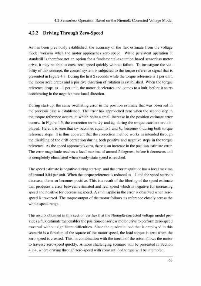
4.2 Sensorless Operation Based on the Niemela-Corrected Voltage Model
4.2.2 Driving Through Zero-Speed
As has been previously established, the accuracy of the flux estimate from the voltagemodel worsens when the motor approaches zero speed. While persistent operation atstandstill is therefore not an option for a fundamental-excitation based sensorless motordrive, it may be able to cross zero-speed quickly without failure. To investigate the via-bility of this concept, the control system is subjected to the torque reference signal that ispresented in Figure 4.3. During the first 2 seconds while the torque reference is 1 per unit,the motor accelerates and a positive direction of rotation is established. When the torquereference drops to −1 per unit, the motor decelerates and comes to a halt, before it startsaccelerating in the negative rotational direction.
During start-up, the same oscillating error in the position estimate that was observed inthe previous case is established. The error has approached zero when the second step inthe torque reference occurs, at which point a small increase in the position estimate erroroccurs. In Figure 4.5, the correction terms kT and kψ during the torque transient are dis-played. Here, it is seen that kT becomes equal to 1 and kψ becomes 0 during both torquereference steps. It is thus apparent that the correction method works as intended throughthe disabling of the drift correction during both positive and negative steps in the torquereference. As the speed approaches zero, there is an increase in the position estimate error.The error magnitude reaches a local maxima of around 5 degrees, before it decreases andis completely eliminated when steady-state speed is reached.
The speed estimate is negative during start-up, and the error magnitude has a local maximaof around 0.04 per unit. When the torque reference is reduced to−1 and the speed starts todecrease, the error becomes positive. This is a result of the filtering of the speed estimatethat produces a error between estimated and real speed which is negative for increasingspeed and positive for decreasing speed. A small spike in the error is observed when zero-speed is traversed. The torque output of the motor follows its reference closely across thewhole speed range.
The results obtained in this section verifies that the Niemela-corrected voltage model pro-vides a flux estimate that enables the position-sensorless motor drive to perform zero-speedtraversal without significant difficulties. Since the quadratic load that is employed in thisscenario is a function of the square of the motor speed, the load torque is zero when thezero-speed is crossed. This, in combination with the inertia of the rotor, allows the motorto traverse zero-speed quickly. A more challenging scenario will be presented in Section4.2.4, where driving through zero-speed with constant load torque will be attempted.
63

Chapter 4. Real-Time Simulation Results
(a) Estimated and measured rotor position. (b) Rotor position estimate error.
(c) Estimated and measured rotor speed. (d) Rotor speed estimate error.
(e) Estimated output torque and torque reference.
Figure 4.3: Driving through zero-speed with the Niemela-corrected voltage model.
64
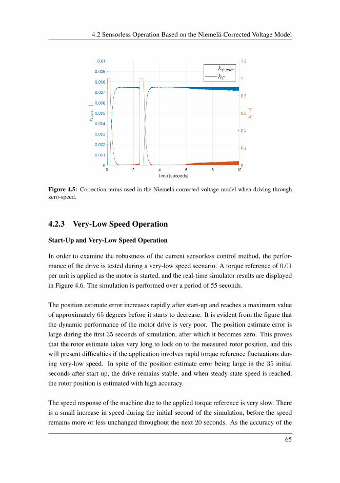
4.2 Sensorless Operation Based on the Niemela-Corrected Voltage Model
Figure 4.5: Correction terms used in the Niemela-corrected voltage model when driving throughzero-speed.
4.2.3 Very-Low Speed Operation
Start-Up and Very-Low Speed Operation
In order to examine the robustness of the current sensorless control method, the perfor-mance of the drive is tested during a very-low speed scenario. A torque reference of 0.01
per unit is applied as the motor is started, and the real-time simulator results are displayedin Figure 4.6. The simulation is performed over a period of 55 seconds.
The position estimate error increases rapidly after start-up and reaches a maximum valueof approximately 65 degrees before it starts to decrease. It is evident from the figure thatthe dynamic performance of the motor drive is very poor. The position estimate error islarge during the first 35 seconds of simulation, after which it becomes zero. This provesthat the rotor estimate takes very long to lock on to the measured rotor position, and thiswill present difficulties if the application involves rapid torque reference fluctuations dur-ing very-low speed. In spite of the position estimate error being large in the 35 initialseconds after start-up, the drive remains stable, and when steady-state speed is reached,the rotor position is estimated with high accuracy.
The speed response of the machine due to the applied torque reference is very slow. Thereis a small increase in speed during the initial second of the simulation, before the speedremains more or less unchanged throughout the next 20 seconds. As the accuracy of the
65

Chapter 4. Real-Time Simulation Results
position estimate improves, the speed starts to increase and steady-state speed is reachedafter approximately 40 seconds of simulation. The inability of the drive to accelerate themotor during the first 20 seconds is interesting, and may be a direct result of the inaccurateposition estimate during this period of time. The noise in the speed estimate and torqueoutput of the motor is seen to become substantial during low-speed operation.
(a) Estimated and measured rotor position. (b) Rotor position estimate error.
(c) Estimated and measured rotor speed. (d) Rotor speed estimate error.
(e) Estimated output torque and torque reference.
Figure 4.6: Start-up and very-low speed operation using the Niemela-corrected voltage model.
66

4.2 Sensorless Operation Based on the Niemela-Corrected Voltage Model
Very-Low Speed Operation With High Initial Speed
It is evident that the accuracy of the position estimate is poor initially if the drive is givena small torque reference when it is at a standstill. It is hypothesized that the drive’s abilityto operate at low speed will be better if the motor is already operating at high speed whenthe torque reference of 0.01 per unit is applied. To investigate this, the motor is broughtto a steady-state speed of around 1 per unit by applying a torque reference of 1 per unit,before the torque reference is reduced to 0.01 per unit.
The results from this scenario are displayed in Figure 4.7. Here, it is seen that if themotor speed already is high when the torque reference of 0.01 per unit is given, the ac-curacy of the position and speed estimation is very good during the transient followingthe torque reference step. The error in the position estimate has a peak value of around 2
degrees and is quickly reduced to a mean value of 0 degrees as the steady-state speed isapproached. There is however considerable noise present in the position estimate as thespeed is reduced. The speed estimate error is seen to have an initial value of around 0.01
per unit, which is reduced to almost 0 as steady-state is approached. This is an interestingobservation, as it suggests that the the steady-state error in the speed estimate is larger forhigh speeds than for low speeds.
The results in this section indicate that very-low speed operation when using the Niemela-corrected voltage model for flux estimation is a viable option. The drive seems to struggleif it initially is at a standstill when the small torque reference is applied, but in spite ofthe large position error during the start-up transient and the very slow speed response fol-lowing the torque reference step, the motor drive remains stable and performs well duringsteady-state. If the motor is operated at high speed initially, the accuracy of the method isvery good during the transient following the torque reference step, and estimation is donewith almost perfect accuracy. Very-low speed operation thus only seems to be problematicif the motor has zero speed initially.
67
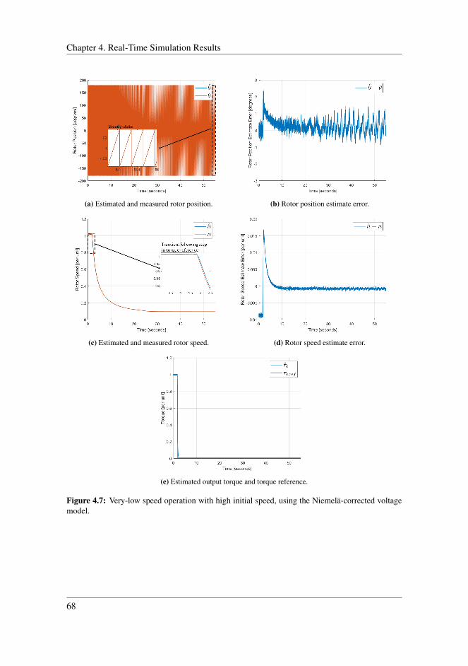
Chapter 4. Real-Time Simulation Results
(a) Estimated and measured rotor position. (b) Rotor position estimate error.
(c) Estimated and measured rotor speed. (d) Rotor speed estimate error.
(e) Estimated output torque and torque reference.
Figure 4.7: Very-low speed operation with high initial speed, using the Niemela-corrected voltagemodel.
68

4.2 Sensorless Operation Based on the Niemela-Corrected Voltage Model
4.2.4 Driving Through Zero-Speed With Constant Load Torque
In Section 4.2.2, it was shown that the motor is capable of crossing zero-speed withoutnoteworthy difficulties when the load torque is a quadratic function of the speed. Whenthe motor is at a standstill, the quadratic load function becomes zero, which enables themotor to traverse the zero-speed region quickly. In this section, a more challenging operat-ing scenario is investigated. Here, a constant load torque will be applied, such that the loadtorque is non-zero during the zero-speed drive-through. This load characteristics is typicalfor hoists and cranes, where the load torque will remain the same, independent of speedmagnitude and direction [37]. The load torque is set equal to 0.2 per unit throughout theduration of the simulation. The motor torque reference is set equal to 0.3 per unit duringthe first 9 seconds, before it is reduced to 0.1 for the remainder of the simulation. Thismeans that the difference between load torque and motor torque will be equal to 0.1 perunit at most, which means that the motor will both accelerate and drive through zero-speedslowly.
The real-time simulation results can be seen in Figure 4.8. In the moments immediately af-ter start-up, the torque output of the motor is increasing from 0 towards its reference value,while the load torque is equal to 0.3 per unit. This results in the motor speed becomingnegative initially, as the load torque is larger than the torque output for a short period oftime. When the torque output of the machine exceed the magnitude of the load torque, themotor decelerates and eventually drives through zero-speed after roughly 6 seconds. Thespeed is now positive. When the torque reference is reduced to 0.1 per unit after 9 seconds,the motor decelerates and drives through zero-speed again, making the speed become neg-ative. In this scenario, the machine operates as a generator when the speed is negative andas a motor when the speed is positive.
The position estimate is inaccurate immediately after start-up, but the error is quickly re-duced. During both zero-speed drive-throughs, the estimate becomes inaccurate for a shortperiod of time, with errors becoming in excess of 20 degrees and 10 degrees, respectively.However, the drive perform both speed-reversals with ease, although the position estimateerrors are larger than when zero-speed drive-through with a quadratic load function wasperformed. This verifies that speed-reversals with a constant load torque presents a morechallenging scenario.
The results in this section indicate that the methods based on the Niemela-corrected volt-age model is an option also for applications that require a constant load torque.
69

Chapter 4. Real-Time Simulation Results
(a) Estimated and measured rotor position. (b) Rotor position estimate error.
(c) Estimated and measured rotor speed. (d) Rotor speed estimate error.
(e) Estimated output torque and torque reference.
Figure 4.8: Driving through zero-speed with constant load torque, using the Niemela-correctedvoltage model.
70
4.3 Sensorless Operation Based on the Voltage-Current Model
4.3 Sensorless Operation Based on the Voltage-CurrentModel
In the preceding section, it was established that sensorless operation based on the Niemela-corrected voltage model is a viable option across the majority of the speed-range. In thissection, the performance of the voltage-current model that was presented in Section 3.5will be examined.
The voltage-current model based sensorless drive will be tested in the same operatingscenarios as the Niemela-corrected voltage model was tested in: Nominal operation, driv-ing through zero-speed, very-low speed operation and driving through zero-speed withconstant load torque. This way, comparisons between the two methods can be made. Asbefore, the resistance is estimated 20% too low during all simulations to induce driftingof the flux estimate and a quadratic, speed-dependent load torque function will be usedinitially.
In this section, the original low-pass filter design for filtering of the speed estimate will beused. This means that the filter time constant will be set equal to 0.005. For the Niemela-corrected voltage model, a large time constant was necessary for the drive to remain stable,but the method based on the voltage-current model does not seem to be very sensitive tonoise in the speed estimate, and a smaller time constant can thus be used.
4.3.1 High-Speed Operation Including Start-Up
Figure 4.9 shows the result from the first 6 seconds of operation after a torque referenceequal to 1 per unit is applied to the control system. The results reveal that the methodbased on the voltage-current model manages to estimate the rotor position with high accu-racy throughout the duration of the simulation, with a peak in the estimate error occurringafter start-up. In the moments following start-up, the error in the estimate increases andreaches a maximum value of less than 8 degrees. The error magnitude quickly decays,and as steady-state is approached, the error is eliminated. In comparison with the methodbased on the Niemela-corrected voltage model, the start-up error in the position estimatefrom when using the voltage-current model is considerably smaller. The time necessaryfor the error to reach its steady-state value of approximately 0 degrees is similar in bothcases.
The speed estimate error has small oscillations during start-up, before it reaches its steady-state value that has a small negative offset because of the difference between the measured
71

Chapter 4. Real-Time Simulation Results
speed and estimated speed due to the low-pass filtering of the latter. The speed estimateis considerably more noisy than when the Niemela-corrected voltage model was used, asthis method required a much larger filter time constant, bu the dynamics of the estimateis however much faster. The torque output of the machine follows its reference value,with a small amount of noise being present in steady-state due to the noise in the positionestimate.
72

4.3 Sensorless Operation Based on the Voltage-Current Model
(a) Estimated and measured rotor position. (b) Rotor position estimate error.
(c) Estimated and measured rotor speed. (d) Rotor speed estimate error.
(e) Estimated output torque and torque reference.
Figure 4.9: Start-up and high speed operation using the voltage-current model.
4.3.2 Driving Through Zero-Speed
To examine the performance of the voltage-current model around zero speed, the torquereference is set equal to 1 per unit during the first two seconds of simulation, before it isreduced to −1 per unit during the remainder of the simulation.
73

Chapter 4. Real-Time Simulation Results
From the results in Figure 4.10 it is seen that the voltage-current model is capable ofdriving through zero speed without noteworthy difficulty. The peak error has a magnitudeof around 9 degrees during the zero-speed drive through, which is higher than the errorwhen the Niemela-corrected voltage model was used. The voltage-current model henceseems to provide a more accurate rotor position estimate during start-up, but does performslightly worse during zero-speed drive through.
The speed estimate is accurate throughout the complete speed range, with a peak errormagnitude of almost 0.015 per unit during the zero-speed drive-through. The torque out-put of the machine follows its reference closely.
74

4.3 Sensorless Operation Based on the Voltage-Current Model
(a) Estimated and measured rotor position. (b) Rotor position estimate error.
(c) Estimated and measured rotor speed. (d) Rotor speed estimate error.
(e) Estimated output torque and torque reference.
Figure 4.10: Driving through zero-speed using the voltage-current model.
75

Chapter 4. Real-Time Simulation Results
4.3.3 Very-Low Speed Operation
Start-Up and Very-Low Speed Operation
The results from the testing of the voltage-current model during start-up and very-lowspeed operation after a torque reference equal to 0.01 per unit was applied are shown inFigure 4.11.
The error in the position estimate is seen to be relatively large during the initial 10 secondsof simulation, reaching a peak value of around 27 degrees. The position estimate is re-duced considerably faster than when the method based on the Niemela-corrected voltagemodel was used, and after approximately 15 seconds, the position error has been reducedto around 2 degrees. This error does however remain in the position estimate throughoutthe remainder of the simulation, and the voltage-current model seems to be incapable ofremoving this steady-state offset with the current tuning of the PI controller in the feed-back loop. It is hypothesized that the error might be the result of insufficient integral effectin the PI controller in the feedback loop, and the integral gain of the controller is increasedin an attempt to remove the offset. The integral gain is increased to point of the observerresponse becoming oscillatory and eventually unstable, with no improvement in the per-formance observed along the way. In an attempt to minimize the magnitude of the offset,the proportional gain of the controller is increased, but this does not yield any improve-ments in the accuracy either. The original tuning of the PI controller with kp = 0.1 andki = 0.1 is hence kept. The steady-state offset in the error is to small to have any majorimpact on the control of the motor, and does therefore not present a significant issue.
76

4.3 Sensorless Operation Based on the Voltage-Current Model
(a) Estimated and measured rotor position. (b) Rotor position estimate error.
(c) Estimated and measured rotor speed. (d) Rotor speed estimate error.
(e) Estimated output torque and torque reference.
Figure 4.11: Start-up and very-low speed operation using the voltage-current model.
77

Chapter 4. Real-Time Simulation Results
Very-Low Speed Operation With High Initial Speed
As when using the Niemela-corrected voltage model, to investigate if the voltage-currentmodel performs better during very-low speed if the initial speed is high, the motor isbrought to steady-state operation at around 1 per unit speed, before the torque reference isreduced to 0.01 per unit. The results from this simulation are shown in Figure 4.12. As inthe case of the Niemela-corrected voltage model, the method based on the voltage-currentmodel is able to estimate the rotor position with high accuracy when the speed is reducedto below 0.1 per unit. It is however seen that the steady-state offset in the position estimatethat was observed previously is established also in this scenario when the speed becomeslow. This suggests that the offset in the position estimate is a result of an inherent weak-ness in the voltage-current model that prevents it from estimating the stator flux perfectlyduring very-low speed operation, which does not depend on whether the motor is startedfrom a standstill or brought to the very-low speed region from an high initial speed.
The speed response of the motor during low-speed operation following start-up is con-siderably better when using the voltage-current model than when the Niemela-correctedvoltage model was used. While the response in the latter case was extremely slow due tothe large error in the position estimate during the first half of the simulation, the voltage-current model based motor drive speeds up immediately after the step in the torque ref-erence. Considering the superior dynamic response of the voltage-current model, thismethod may be a better option than the method based on the Niemela-corrected voltagemodel during very-low speed operation, in spite of the former’s inability to remove thesteady-state error in its position estimate.
78

4.3 Sensorless Operation Based on the Voltage-Current Model
(a) Estimated and measured rotor position. (b) Rotor position estimate error.
(c) Estimated and measured rotor speed. (d) Rotor speed estimate error.
(e) Estimated output torque and torque reference.
Figure 4.12: Very-low speed operation with high initial speed, using the voltage-current model.
79

Chapter 4. Real-Time Simulation Results
4.3.4 Driving Through Zero-Speed With Constant Load Torque
The results from the testing of the zero-speed drive-through capability of the voltage-current model under the influence of a constant load torque are displayed in Figure 4.13.
The error in both position estimate and speed estimate is seen to become very large duringthe initial start-up transient. These errors are however quickly eliminated, and the speedis estimated accurately for the remainder of the simulation. The position estimate erroris quickly eliminated after the start-up transient, but spikes in the error occur during bothzero-speed traversals. Similar to when the Niemela-corrected voltage model was used, theerror is largest during the second zero-speed crossing, when the rotational speed of the mo-tor goes from being positive to becoming negative once again. The error reaches a valueof around 25 and 15 degrees during the first and second zero-speed traversals, respectively.
Slow zero-speed drive-throughs with a constant load torque thus seems to be a manageabletask for the voltage-current model based method as well.
80

4.3 Sensorless Operation Based on the Voltage-Current Model
(a) Estimated and measured rotor position. (b) Rotor position estimate error.
(c) Estimated and measured rotor speed. (d) Rotor speed estimate error.
(e) Estimated output torque and torque reference.
Figure 4.13: Driving through zero-speed with constant load torque, using the voltage-current model.
81

Chapter 4. Real-Time Simulation Results
82

Chapter 5Discussion
In Section 3.1.3 the steady-state sensitivity analysis of the voltage model showed that thestator flux estimate is sensitive to errors in the stator resistance and stator voltage estimateswhen the motor speed is low. In Section 3.4.1 it was shown how such errors will lead toa flux estimate that becomes increasingly inaccurate over time due to the voltage modelerrors being integrated for each time step. These flux estimate errors cause inaccurate rotorposition estimates, which in turn cause inaccurate d- and q-axis current references and afollowing deterioration of the performance of the motor drive. This was verified by thereal-time simulation that was run in Section 4.1, where the motor drive was operated with-out a position sensor. Here, it was demonstrated that with the stator voltage estimated usingthe converter reference voltage and the stator resistance being estimated 20% too low, therotor position estimate becomes increasingly inaccurate over time, eventually causing amalfunction of the motor drive. This shows that modifications of the conventional volt-age model must be implemented in order to achieve a sensorless control algorithm that ispractically feasible. Two alternatives for an improved flux estimate were presented: TheNiemela-corrected voltage model and the voltage-current model.
5.1 Comparison of the Performance of the Flux Models
Both the methods based on the Niemela-corrected voltage model and the voltage-currentmodel were capable of estimating the rotor position with high accuracy during start-upand nominal operation when the torque reference was equal to 1 per unit. While bothmethods eliminated the position estimate error equally fast, the error with the Niemela-corrected method was considerably larger and more oscillatory during start-up than whenthe voltage-current model based method was used. Both methods were able to perform
83

Chapter 5. Discussion
speed-reversals with ease when the torque reference was varied from 1 per unit to −1
per unit, although spikes in the position estimate errors occurred when zero-speed wascrossed. The error during the zero-speed traversal was lowest when using the Niemela-corrected voltage model. The zero-speed traversals in the above scenario were relativefast due to the quadratic load torque function being used: At zero speed, the torque loadbecome zero, allowing the motor to traverse zero-speed very quickly, and to challenge thedrive, slower zero-speed drive-throughs were therefore performed by using a constant loadtorque. The results from these simulations show that both methods struggle more in thisscenario, but both methods were still able to cross zero-speed without significant prob-lems. In this scenario, the accuracy of the position estimate was similar for both methods,but the error was slightly smaller when the Niemela-corrected voltage model was used.
When a very-low torque reference was used, both methods struggled during start-up and ittook a significant amount of time before the position estimate errors were reduced. How-ever, the dynamics when using the voltage-current model were superior to the methodbased on the Niemela-corrected voltage model, with the former clearing the position esti-mate error considerably faster. When the very-low torque reference was applied with themotor already operating at high speed, both methods estimated the rotor position almostperfectly. This shows that start-up and subsequent low-speed operation is a much morechallenging scenario than when the speed is reduced from high speed to very-low speed.During both low-speed scenarios, there was a small steady-state offset in the position es-timate when using the voltage-current model that was not removed even after further tun-ing of the PI controller in the feedback loop of the voltage-current model was attempted.However, this error seems to be too small to have any practical consequences. The inter-mediate results from the trial-and-error based tuning procedure that was employed on thePI controller of the observer are not included in this thesis, but the process revealed thatthe performance of the voltage-current model is highly sensitive to the tuning of the PIcontroller in the feedback loop, with small adjustments in any of the tuning parametersresulting in inability to estimate the rotor position accurately. The controller gains thatwere used in this thesis appear to be optimal values for this specific configuration.
As mentioned in Chapter 4, when using the Niemela-corrected voltage model, the perfor-mance of the drive was highly sensitive to noise in the speed estimate. The time constantof the speed estimate filter had to be increased to 0.06 in order for the drive to remainstable, which resulted in a speed estimate with a small amount of noise, but with relativeslow dynamics. In comparison, a filter constant as low as 0.005 seconds was used forthe voltage-current model. This could present a problem if the drive were to be testedunder speed-controlled operation, where the estimated speed would be used as feedback
84

5.2 General Remarks About Fundamental-Excitation Based Sensorless Control
and compared with the reference speed. If the speed estimate changes considerably slowerthan the real speed due to the filtering, this could lead to deterioration of the drive’s per-formance and potentially instability.
The simulations in this thesis were performed with a resistance value that was underesti-mated with 20% in order to emulate a scenario in which flux models with drift-correctioncapabilities are necessary. Due to the temperature-dependency of the stator resistance,having a real stator resistance value that differs from the estimated value is a very likelyscenario, and the simulations in this thesis can therefore be deemed applicable for situa-tions that may be encountered in the real world. All other motor parameters were assumedto be accurately measured, although the estimated values of the permanent magnet fluxlinkage and the motor inductances in practice also will differ from their real values. Thismay be particularly problematic for the voltage-current model that relies not only on thevoltage model, but also on the current model, in which these parameter values are included.In the case of erroneously estimated inductances and permanent magnet flux linkage, theflux reference provided by the current model in the voltage-current model would differfrom the real flux, which would results in an error being fed back to the voltage modeleven if the voltage model flux estimate was accurate. Such a scenario would most likelyworsen the performance of the voltage-current model. The fact that the Niemela-correctedvoltage model only relies on a single motor paramater, namely the stator resistance, whilethe voltage-current model relies on the stator resistance, stator inductances and permanentmagnet flux linkage could be an advantage of the former. This can be verified throughsimulations in which also the inductances and the permanent magnet flux linkage are er-roneously estimated.
5.2 General Remarks About Fundamental-Excitation BasedSensorless Control
The sensorless control methods that have been investigated in this thesis are both basedon the voltage model, and do hence fall within the fundamental-excitation based meth-ods category. While such methods typically struggle around zero-speed, the simulationresults that are obtained in this thesis indicate that both the method based on the Niemela-corrected voltage model and the method based on the voltage-current model perform sat-isfactory during zero-speed traversals, and are even able to remain stable during persistentoperation at speeds below 0.1 per unit. For applications that require very high accuracy in
85

Chapter 5. Discussion
the very-low speed region, saliency tracking methods such as the high-frequency signal-injection method that is presented in Appendix G may have to be implemented. This wouldadd complexity and cost to the drive system, and considering that persistent very-low speedoperation may not be a common scenario in most applications, cost-benefit analysis wouldbe necessary to determine whether or not such additional methods should be implemented.The results obtained from the real-time simulations in this thesis demonstrate that the FE-based methods that were implemented in this thesis are satisfactory accurate for scenariosthat include start-up, medium and high-speed operation and zero-speed drive-throughs,and are even capable of persistent very-low speed operation. Additionally, the methodswere proven to be effective for both speed-dependent and constant load torques, makingthe proposed methods viable options across most of the speed range for a broad range ofapplications, including pumps, fans, hoists and cranes.
5.3 The ERTS and Assessment of Result Validity
Ideally, the control software that was developed in this thesis would have been verifiedexperimentally on a physical laboratory setup. The development of a fully functioningPMSM drive test bench is an ongoing effort within the PESC group in the Department ofElectric Power Engineering at NTNU, but due to delays caused by the ongoing Covid-19pandemic, it has not yet been made available. This thesis has hence relied solely on theFPGA-based ERTS for control software verification. The ERTS has proved to be a usefultool for verification of the C++-based control software without having access to a physicalmotor drive setup. In addition to providing a means of software-in-the loop testing andfinal verification of the control software, the real-time nature of its simulations, due thehigh processing capability of the FPGA, has made it possible to investigate the long-timedynamics of the position-sensorless motor drive. This was useful when the performanceof the position-sensorless motor drive was investigated during very-low speed operation,when simulations with a duration of 55 seconds were performed. Performing similar sim-ulations with conventional simulation tools such as MATLAB Simulink would be a highlytime-consuming effort, making the ERTS tool an invaluable asset in the development andverification of sensorless control methods.
The accuracy of the ERTS was investigated by Perera et. al in [45], where the PMSMdrive hardware emulator was compared to an equivalent MATLAB Simulink model. Theresults from this analysis showed negligible numerical errors in d- and q-axis currents,rotor position estimate and torque output between the ERTS and the MATLAB Simulink
86

5.3 The ERTS and Assessment of Result Validity
model during a 1 second simulation run. This indicates that the accuracy of the ERTS ishigh, and it is hence reasonable to trust the results that are obtained in this thesis with arelatively high degree of certainty. The ERTS performed the 1 second simulation in real-time, while the run-time of the Simulink model was in the vicinity of 550 seconds. Theusefulness of the ERTS as a tool is thus evident: Using it, simulations can be considerablyaccelerated at the expense of practically insignificant numerical errors.
87

Chapter 5. Discussion
88

Chapter 6Conclusion and Further Work
6.1 Conclusion
In this thesis, C++ software that enables sensorless indirect torque control of a permanentmagnet synchronous machine has been successfully developed and implemented using astate-of-the-art SoC-based embedded control platform. The validity of the control strate-gies has been verified using an FPGA-based embedded real-time simulator.
Two different flux models have been used in combination with the active flux conceptto facilitate position-sensorless operation: The Niemela-corrected voltage model and thevoltage-current model. Both flux estimation methods have enabled sensorless operationacross the majority of the speed range when the stator resistance is erroneously estimated,and have performed well during scenarios that include start-up and high speed operationand zero-speed drive-throughs. Moreover, very-low speed operation below 0.1 per unitspeed has also proved to be a viable option. By performing tests with both quadratic andconstant load functions, the methods have been verified for several applications, such asfans, pumps, hoists and cranes.
In general, the method based on the Niemela-corrected voltage model and the voltage-current model have performed similarly. The method based on the voltage-current modelseems to be capable of removing errors in the position estimate considerably faster thanthe one based on the Niemela-corrected voltage model. In return, its steady-state positionestimate seems to be less accurate, containing a small steady-state offset of around 1-2degrees when the speed is low. A potential drawback of the method based on the Niemela-corrected voltage model is that it requires aggressive filtering of speed estimate to remain
89

Chapter 6. Conclusion and Further Work
stable. This could present difficulties if the drive were to be speed-controlled, as the largelow-pass filter time constant results in a speed estimate that changes notably slower thanthe actual rotor speed during transients. However, this did not seem to have any signif-icant negative impact on the torque-controlled drive. In conclusion, it can be stated thatthe Niemela-corrected voltage model and the voltage-current model in combination withthe active flux concept both provide well-performing fundamental-excitation based torquecontrolled sensorless PMSM drives. Which flux model to use may become a trade-off be-tween fast dynamic response and steady-state accuracy. Both methods are able to operateacross the majority of the speed range for a broad range of applications.
The FPGA-based ERTS has proved to be an invaluable tool in the development of motorcontrol software. Using it, software-in-the-loop testing has been made possible, enablingfrequent testing of the motor control strategies. In this thesis, it has also been used for finalverification of the proposed C++ control software, due to the lack of a fully functioningPMSM drive test bench. Additionally, its real-time nature has made the production of whatcan be assumed to be highly accurate results a considerably less time-consuming than ifconventional simulations tools were to be used.
6.2 Further Work
The following suggestions for further work are made:
6.2.1 Software Verification on a Physical Laboratory Setup
The control software that was developed in this thesis has relied solely on the ERTS forverification. Although the ERTS can be trusted to produce high-accuracy results, testingof the control strategies on a physical laboratory setup would provide final validation ofthe concepts that have been proposed, and should thus be performed.
As previously discussed, the PMSM drive test bench that is currently being developmentby the PESC group in the Department of Electric Power Engineering was not made avail-able during the work with this thesis due to delays caused by the Covid-19 pandemic, butit is likely that it will be available for future candidates.
6.2.2 Improving the Performance of the Position-Sensorless Drive
In Section 3.6, two strategies for improvement of the performance of the sensorless motordrive were presented:
90

6.2 Further Work
• Including a PLL for rotor position filtering
• Implementing high-frequency signal-injection for saliency tracking and improvedstandstill and low-speed performance
The implementation of the above methods may boost the performance of the PMSM drive.Both of the above strategies were attempted implemented in this thesis without success.The approaches that were used are presented in Appendix F and Appendix G, and futureattempts of implementation could use the theory here as a starting point.
Another interesting concept for improved performance of the position-sensorless PMSMdrive is:
• Implementing online parameter estimation algorithms in order to obtain more accu-rate motor parameter estimates in real-time.
6.2.3 Further Testing of the Position-Sensorless Drive
The following scenarios were not investigated in this thesis, and may be tested in thefuture:
• Simulating the position-sensorless drive during speed-controlled operation.
• Simulating scenarios with erroneously estimated permanent magnet flux linkage andstator inductances to investigate how they affect the performance of the voltage-current model.
91

Chapter 6. Conclusion and Further Work
92

Bibliography
[1] F. Alvarez-Gonzalez, A. Griffo, B. Sen, and J. Wang. Real-Time Hardware-in-the-Loop Simulation of Permanent-Magnet Synchronous Motor Drives Under StatorFaults. IEEE Transactions on Industrial Electronics, 64(9):6960–6969, 2017.
[2] G.-D. Andreescu, C. I. Pitic, F. Blaabjerg, and I. Boldea. Combined flux observerwith signal injection enhancement for wide speed range sensorless direct torque con-trol of ipmsm drives. IEEE Transactions on Energy Conversion, 23(2):393–402,2008.
[3] L. G. Barbosa Rolim, D. Rodrigues da Costa, and M. Aredes. Analysis and softwareimplementation of a robust synchronizing pll circuit based on the pq theory. IEEETransactions on Industrial Electronics, 53(6):1919–1926, 2006.
[4] F. Bauer and H. D. Heining. Quick response space vector control for a high powerthree-level-inverter drive system. Archiv fur Elektrotechnik, 74(1):53–59, 1990.
[5] F. Blaschke. The Principle of Field Orientation as Applied to the New TransvectorClosed Loop Control System for Rotating Field Machines. Siemens Review, 34:217–220, 1972.
[6] I. Boldea. Electric generators and motors: An overview. CES Transactions on Elec-trical Machines and Systems, 1(1):3–14, 2017.
[7] I. Boldea and S. C. Agarlita. The active flux concept for motion-sensorless unifiedAC drives: A review. In International Aegean Conference on Electrical Machinesand Power Electronics and Electromotion, Joint Conference, pages 1–16, 2011.
[8] I. Boldea, M. C. Paicu, G. D. Andreescu, and F. Blaabjerg. “Active flux” orienta-
93

tion vector sensorless control of IPMSM. In 2008 11th International Conference onOptimization of Electrical and Electronic Equipment, pages 161–168, 2008.
[9] M. Bolstad. Sensorless Control of Synchronous Machines Used in Adjustable SpeedHydro. Master’s thesis, Department of Electric Power Engineering, NTNU – Nor-wegian University of Science and Technology, June 2018.
[10] Y. Chen and V. Dinavahi. Digital Hardware Emulation of Universal Machine andUniversal Line Models for Real-Time Electromagnetic Transient Simulation. IEEETransactions on Industrial Electronics, 59(2):1300–1309, 2012.
[11] M. Chinchilla, S. Arnaltes, and J. Burgos. Control of permanent-magnet generatorsapplied to variable-speed wind-energy systems connected to the grid. IEEE Trans-actions on Energy Conversion, 21(1):130–135, 2006.
[12] R. S. Colby and D. W. Novotny. An Efficiency-Optimizing Permanent-Magnet Syn-chronous Motor Drive. IEEE Transactions on Industry Applications, 24(3):462–469,1988.
[13] M. Depenbrock. Direct Self-Control (DSC) of Inverter-Fed Induction Machine. IEEETransactions on Power Electronics, 3(4):420–429, 1988.
[14] C. Dufour, J. Belanger, S. Abourida, and V. Lapointe. FPGA-Based Real-Time Sim-ulation of Finite-Element Analysis Permanent Magnet Synchronous Machine Drives.In 2007 IEEE Power Electronics Specialists Conference, pages 909–915, 2007.
[15] M. Ehsani, K. Rahman, and H. Toliyat. Propulsion system design of electric andhybrid vehicles. IEEE Transactions on Industrial Electronics, 44(1):19–27, 1997.
[16] V. M. Fjellanger. On-Line Voltage Estimation During Sensorless Control of an In-duction Machine Drive. Master’s thesis, Department of Electric Power Engineering,NTNU – Norwegian University of Science and Technology, June 2019.
[17] B. Fossen. Modelling and Identification of Multi-Phase Machines. Project report inTET4520, Department of Electric Power Engineering, NTNU – Norwegian Univer-sity of Science and Technology, December 2016.
[18] F. M. Gardner. Phaselock Techniques. John Wiley Sons, 2nd edition, 2005.
[19] J. Holtz. Sensorless control of induction machines—with or without signal injection?IEEE Transactions on Industrial Electronics, 53(1):7–30, 2006.
[20] L. I. Iepure, I. Boldea, and F. Blaabjerg. Hybrid I-f Starting and Observer-BasedSensorless Control of Single-Phase BLDC-PM Motor Drives. IEEE Transactions onIndustrial Electronics, 59(9):3436–3444, 2012.
94
[21] Y. Inaba, S. Cense, T. O. Bachir, H. Yamashita, and C. Dufour. A Dual High-SpeedPMSM Motor Drive Emulator With Finite Element Analysis on FPGA Chip WithFull Fault Testing Capability. In Proceedings of the 2011 14th European Conferenceon Power Electronics and Applications, pages 1–10, 2011.
[22] International Energy Agency. World Energy Outlook 2020. 2020.
[23] A. Jack, B. Mecrow, and J. Haylock. A comparative study of permanent magnet andswitched reluctance motors for high-performance fault-tolerant applications. IEEETransactions on Industry Applications, 32(4):889–895, 1996.
[24] T. M. Jahns, G. B. Kliman, and T. W. Neumann. Interior Permanent-Magnet Syn-chronous Motors for Adjustable-Speed Drives. IEEE Transactions on Industry Ap-plications, IA-22(4):738–747, 1986.
[25] P. Jansen and R. Lorenz. A physically insightful approach to the design and accu-racy assessment of flux observers for field oriented induction machine drives. IEEETransactions on Industry Applications, 30(1):101–110, 1994.
[26] I. N. Jensen. Control of an Ironless Permanent Magnet Synchronous Machine.Project report in TET4520, Department of Electric Power Engineering, NTNU –Norwegian University of Science and Technology, December 2020.
[27] Jun Hu and Bin Wu. New integration algorithms for estimating motor flux over awide speed range. IEEE Transactions on Power Electronics, 13(5):969–977, 1998.
[28] S. Kim, J.-I. Ha, and S.-K. Sul. PWM Switching Frequency Signal Injection Sensor-less Method in IPMSM. IEEE Transactions on Industry Applications, 48(5):1576–1587, 2012.
[29] K. P. Kovacs and M. Kuzniarski. Transiente Vorgange In Wechselstrommaschinen.Verlag der Ungarischen Akademie der Wissenschaften, 2nd edition, 1959.
[30] C. Lascu, I. Boldea, and F. Blaabjerg. Super-twisting sliding mode control of torqueand flux in permanent magnet synchronous machine drives. In IECON 2013 - 39thAnnual Conference of the IEEE Industrial Electronics Society, pages 3171–3176,2013.
[31] M. Linke, R. Kennel, and J. Holtz. Sensorless speed and position control of syn-chronous machines using alternating carrier injection. In IEEE International ElectricMachines and Drives Conference, 2003. IEMDC’03., volume 2, pages 1211–1217vol.2, 2003.
95
[32] J. Luukko. Direct Torque Control of Permanent Magnet Synchronous Machines -Analysis and Implementation. PhD thesis, Lappeenranta University of Technology,2000.
[33] H. L. Mjell. Sensorless Control of Synchronous Machines Used in ASH. Master’sthesis, Department of Electric Power Engineering, NTNU – Norwegian Universityof Science and Technology, June 2019.
[34] N. Mohan, T. M. Undeland, and W. P. Robbins. Power Electronics: Converters,Applications, and Design. John Wiley Sons, 2nd edition, 1995.
[35] A. Moldskred. FPGA-Based Real-Time Emulator of Permanent Magnet Syn-chronous Motor. Master’s thesis, Department of Electric Power Engineering, NTNU– Norwegian University of Science and Technology, June 2020.
[36] M. Niemela. Position Sensorless Electrically Excited Synchronous Motor Drivefor Industrial Use Based on Direct Flux Linkage and Torque Control. PhD thesis,Lappeenranta University of Technology, 1999.
[37] R. Nilsen. Electric Drives. Norwegian University of Science and Technology, 2018.
[38] R. Nilsen. Modeling, Identification and Control of Electrical Machines. NorwegianUniversity of Science and Technology, 2019.
[39] M. D. Omar Faruque, T. Strasser, G. Lauss, V. Jalili-Marandi, P. Forsyth, C. Dufour,V. Dinavahi, A. Monti, P. Kotsampopoulos, J. A. Martinez, K. Strunz, M. Saeedifard,X. Wang, D. Shearer, and M. Paolone. Real-Time Simulation Technologies for PowerSystems Design, Testing, and Analysis. IEEE Power and Energy Technology SystemsJournal, 2(2):63–73, 2015.
[40] M. C. Paicu, I. Boldea, G. . Andreescu, and F. Blaabjerg. Very Low Speed Perfor-mance of Active Flux Based Sensorless Control: Interior Permanent Magnet Syn-chronous Motor Vector Control Versus Direct Torque and Flux Control. IET ElectricPower Applications, 3(6):551–561, 2009.
[41] M. C. Paicu, L. Tutelea, I. Boldea, G. D. Andreescu, and R. Ancuti. Pm-rsm sen-sorless vector control: Zero q-axis flux versus approximate maximum torque percurrent, with experiments. In 2010 12th International Conference on Optimizationof Electrical and Electronic Equipment, pages 460–468, 2010.
[42] A. Perera and R. Nilsen. A Sensorless Control Method for IPMSM with an Open-Loop Predictor for Online Parameter Identification. In 2020 23rd International Con-ference on Electrical Machines and Systems (ICEMS), pages 1983–1988, 2020.
96
[43] A. Perera and R. Nilsen. Gauss-Newton: A Prediction-Error-Gradient based Algo-rithm to Track PMSM Parameters Online. In 2020 IEEE International Conferenceon Power Electronics, Drives and Energy Systems (PEDES), pages 1–8, 2020.
[44] A. Perera and R. Nilsen. Full Speed Range Sensorless IPMSM Drive Enhancedwith Online Parameter Identification. IEEE International Electric Machines DrivesConference (IEMDC), page 6, 2021.
[45] A. Perera, R. Nilsen, T. Haugan, and K. Ljøkelsøy. A Design Method of an Em-bedded Real-Time Simulator for Electric Drives using Low-Cost System-on-ChipPlatform. PCIM Europe digital days, In Press, page 8, 2021.
[46] P. D. C. Perera, F. Blaabjerg, J. K. Pedersen, and P. Thogersen. A Sensorless, Sta-ble V/f Control Method for Permanent-Magnet Synchronous Motor Drives. IEEETransactions on Industry Applications, 39(3):783–791, 2003.
[47] P. Pillay and R. Krishnan. Modeling, simulation, and analysis of permanent-magnetmotor drives. i. the permanent-magnet synchronous motor drive. IEEE Transactionson Industry Applications, 25(2):265–273, 1989.
[48] I. Takahashi and T. Noguchi. A New Quick-Response and High-Efficiency ControlStrategy of an Induction Motor. IEEE Transactions on Industry Applications, IA-22(5):820–827, 1986.
[49] P. Weichbold and T. V. Raumer. Influence of Dead Time Effects of PWM-VSI onCurrent Control. 2001.
[50] R. Wu and G. R. Slemon. A permanent magnet motor drive without a shaft sensor.IEEE Transactions on Industry Applications, 27(5):1005–1011, 1991.
[51] S.-C. Yang and Y.-L. Hsu. Full speed region sensorless drive of permanent-magnetmachine combining saliency-based and back-emf-based drive. IEEE Transactionson Industrial Electronics, 64(2):1092–1101, 2017.
[52] Y.-D. Yoon, S.-K. Sul, S. Morimoto, and K. Ide. High-Bandwidth Sensorless Al-gorithm for AC Machines Based on Square-Wave-Type Voltage Injection. IEEETransactions on Industry Applications, 47(3):1361–1370, 2011.
97

98

Appendix AThe Inductance Matrix
Since the stator flux path changes with rotor position in the IPMSM, the stator inductancematrix becomes a function of the rotor electrical position θ. The inductance matrix can bewritten as the sum of a leakage inductance matrix, a position independent inductance ma-trix and a position dependent matrix [38]. The complete stator inductance matrix becomes
Lss =
Lsσ + Lsm + Lg cos (2θ) − 12Lsm + Lg cos (2θ − 2π
3 )
− 12Lsm + Lg cos (2θ − 2π
3 ) Lsσ + Lsm + Lg cos (2θ + 2π3 )
− 12Lsm + Lg cos (2θ + 2π
3 ) − 12Lsm + Lg cos (2θ)
. . .
. . .
− 12Lsm + Lg cos (2θ + 2π
3 )
− 12Lsm + Lg cos (2θ)
Lsσ + Lsm + Lg cos (2θ − 2π3 )
(A.1)
If the machine is non-salient, the air gap of the machine is constant for every value of θ.In that case, Lg will be equal to zero, and the inductance matrix becomes position inde-pendent. The inductance matrix is then
Lss =
Lsσ + Lsm − 12Lsm − 1
2Lsm
− 12Lsm Lsσ + Lsm − 1
2Lsm
− 12Lsm − 1
2Lsm Lsσ + Lsm
(A.2)
99

100

Appendix BMotor Drive Data
Symbol Value UnitNominal Voltage Un 220 VNominal Current In 51 ANominal Frequency fn 35 HzPole pairs p 1 -Nominal Speed Nn 2100 rpmSwitching Frequency fs 4000 HzStator resistance rs 0.009 per-unitd-axis Reactance xd 0.4 per-unitq-axis Reactance xq 1.0 per-unitPermanent Magnet Flux Linkage ψm 0.66 per-unit
101

102
Appendix CBase-Values Used for Per-UnitConversion
Ubasis =
√2
3Un
Ibasis =√
2In
Ψbasis =Ubasis2πfn
Sbasis =√
3UnIn
Tbasis =SbasisNn · π30
103

104

Appendix DScripts Used for Flux ModelSensitivity Analysis
In the below scripts, the maximum-torque-per-ampere control strategy is implemented byassuming current references according to Equation 2.26 and Equation 2.27. The scriptscalculate and compare actual stator flux with estimated flux for speeds and torque ref-erences between −1 and 1 per unit. Flux estimation is hence only performed in themaximum-torque-per-ampere region, meaning that the flux models’ performance duringfield weakening operation has not been considered.
D.1 MATLAB Script for Voltage Model Sensitivity Anal-ysis
1 clc
2 clear all
3
4 % Defining motor parameters
5 x_q = 1;
6 x_d = 0.4;
7 r_s = 0.009;
8 psi_m = 0.66;
9
10 % Performing calculations for torque references between -1 and 1 pu and
11 % speeds between -1 and 1 pu
12 t =[-1:0.05:1];
13 n_vec =[-1:0.05:1];
105
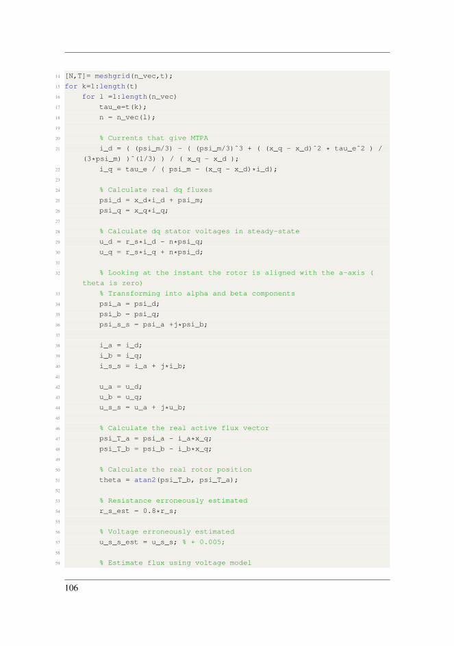
14 [N,T]= meshgrid(n_vec,t);
15 for k=1:length(t)
16 for l =1:length(n_vec)
17 tau_e=t(k);
18 n = n_vec(l);
19
20 % Currents that give MTPA
21 i_d = ( (psi_m/3) - ( (psi_m/3)ˆ3 + ( (x_q - x_d)ˆ2 * tau_eˆ2 ) /
(3*psi_m) )ˆ(1/3) ) / ( x_q - x_d );
22 i_q = tau_e / ( psi_m - (x_q - x_d)*i_d);
23
24 % Calculate real dq fluxes
25 psi_d = x_d*i_d + psi_m;
26 psi_q = x_q*i_q;
27
28 % Calculate dq stator voltages in steady-state
29 u_d = r_s*i_d - n*psi_q;
30 u_q = r_s*i_q + n*psi_d;
31
32 % Looking at the instant the rotor is aligned with the a-axis (
theta is zero)
33 % Transforming into alpha and beta components
34 psi_a = psi_d;
35 psi_b = psi_q;
36 psi_s_s = psi_a +j*psi_b;
37
38 i_a = i_d;
39 i_b = i_q;
40 i_s_s = i_a + j*i_b;
41
42 u_a = u_d;
43 u_b = u_q;
44 u_s_s = u_a + j*u_b;
45
46 % Calculate the real active flux vector
47 psi_T_a = psi_a - i_a*x_q;
48 psi_T_b = psi_b - i_b*x_q;
49
50 % Calculate the real rotor position
51 theta = atan2(psi_T_b, psi_T_a);
52
53 % Resistance erroneously estimated
54 r_s_est = 0.8*r_s;
55
56 % Voltage erroneously estimated
57 u_s_s_est = u_s_s; % + 0.005;
58
59 % Estimate flux using voltage model
106

60 psi_s_s_est = (u_s_s_est - (r_s_est*i_s_s))/(j*n);
61
62 psi_a_est = real(psi_s_s_est);
63 psi_b_est = imag(psi_s_s_est);
64
65 psi_d_est = psi_a_est;
66 psi_q_est = psi_b_est;
67
68 % Estimate active flux
69 psi_T_a_est = psi_a_est - i_a*x_q;
70 psi_T_b_est = psi_b_est - i_b*x_q;
71
72 % Estimate the rotor position
73 theta_est = atan2(psi_T_b_est, psi_T_a_est);
74
75 % Theta error
76 theta_error(k,l) = theta_est*(180/pi);
77 if n==0
78 theta_error(k,l) =0/0;
79 end
80
81 % Flux error
82 flux_mag_error(k,l) = abs(psi_s_s) - abs(psi_s_s_est);
83 flux_angle_error(k,l) = angle(psi_s_s)*(180/pi) - angle(
psi_s_s_est)*(180/pi);
84 if n==0
85 flux_mag_error(k,l) = 0/0;
86 flux_angle_error(k,l) =0/0;
87 end
88
89 % Torque error
90 torque_error(k,l) = ((psi_d-psi_d_est)*i_q - (psi_q - psi_q_est)*i_d);
91 end
92 end
93
94 figure(1)
95 surf(N,T,flux_mag_error)
96 colorbar
97 xlabel(’Speed [pu]’)
98 ylabel(’Torque Reference [pu]’)
99 zlabel (’Flux Amplitude Error [pu]’)
100
101 figure(2)
102 surf(N,T,flux_angle_error)
103 colorbar
104 xlabel(’Speed [pu]’)
105 ylabel(’Torque Reference [pu]’)
107

106 zlabel (’Flux Angle Error [degrees]’)
107
108 figure(3)
109 surf(N,T,torque_error)
110 colorbar
111 xlabel(’Speed [pu]’)
112 ylabel(’Torque Reference [pu]’)
113 zlabel (’Torque Error [pu]’)
114
115 figure(4)
116 surf(N,T,theta_error)
117 colorbar
118 xlabel(’Speed [pu]’)
119 ylabel(’Torque Reference [pu]’)
120 zlabel ([’Theta Error [degrees]’])
121
122 % NB: Field weakening is not considered.
123 % No limits have been considered (limit current and voltage to within
124 % maximum values
Listing D.1: Script for voltage model sensitivity analysis.
D.2 MATLAB Script for Current Model Sensitivity Anal-ysis
1 clc
2 clear all
3
4 % Defining motor parameters
5 x_q = 1.0;
6 x_d = 0.4;
7 r_s = 0.009;
8 psi_m = 0.66;
9
10 % Performing calculations for torque references between -1 and 1 pu and
11 % speeds between -1 and 1 pu
12 t =[-1:0.05:1];
13 n_vec =[-1:0.05:1];
14 [N,T]= meshgrid(n_vec,t);
15 for k=1:length(t)
16 for l =1:length(n_vec)
17 tau_e=t(k);
18 n = n_vec(l);
19
20 % Currents that give MTPA
108

21 i_d = ( (psi_m/3) - ( (psi_m/3)ˆ3 + ( (x_q - x_d)ˆ2 * tau_eˆ2 ) /
(3*psi_m) )ˆ(1/3) ) / ( x_q - x_d );
22 i_q = tau_e / ( psi_m - (x_q - x_d)*i_d);
23
24 % Calculate real dq fluxes
25 psi_d = x_d*i_d + psi_m;
26 psi_q = x_q*i_q;
27
28 % Calculate dq stator voltages in steady-state
29 u_d = r_s*i_d - n*psi_q;
30 u_q = r_s*i_q + n*psi_d;
31
32 % Looking at the instant the rotor is aligned with the a-axis
33 % (theta is zero)
34 % Transforming into alpha and beta components
35 psi_a = psi_d;
36 psi_b = psi_q;
37 psi_s_s = psi_a +j*psi_b;
38
39 i_a = i_d;
40 i_b = i_q;
41 i_s_s = i_a + j*i_b;
42
43 u_a = u_d;
44 u_b = u_q;
45 u_s_s = u_a + j*u_b;
46
47 % Calculate the real active flux vector
48 psi_T_a = psi_a - i_a*x_q;
49 psi_T_b = psi_b - i_b*x_q;
50
51 % Calculate the real rotor position
52 theta = atan2(psi_T_b, psi_T_a);
53
54 % Reactance estimates
55 x_d_est = 1.0*x_d;
56 x_q_est = 1.0*x_q;
57
58 % Permanent magnet flux linkage estimate
59 psi_m_est = 0.8*psi_m;
60
61 % Estimate flux using current model
62 psi_d_est = x_d_est*i_d + psi_m_est;
63 psi_q_est = x_q_est*i_q;
64
65 psi_a_est = psi_d_est;
66 psi_b_est = psi_q_est;
67
109

68 psi_s_s_est = psi_a_est + j*psi_b_est;
69
70 % Estimate active flux
71 psi_T_a_est = psi_a_est - i_a*x_q;
72 psi_T_b_est = psi_b_est - i_b*x_q;
73
74 % Estimate the rotor position
75 theta_est = atan2(psi_T_b_est, psi_T_a_est);
76
77 % Theta error
78 theta_error(k,l) = theta_est*(180/pi);
79
80 % Flux error
81 flux_mag_error(k,l) = abs(psi_s_s) - abs(psi_s_s_est);
82 flux_angle_error(k,l) = angle(psi_s_s)*(180/pi) - angle(
psi_s_s_est)*(180/pi);
83
84 % Torque error
85 torque_error(k,l) = ((psi_d-psi_d_est)*i_q - (psi_q - psi_q_est)*i_d);
86 end
87 end
88
89 figure(1)
90 surf(N,T,flux_mag_error)
91 colorbar
92 xlabel(’Speed [pu]’)
93 ylabel(’Torque Reference [pu]’)
94 zlabel (’Flux Amplitude Error [pu]’)
95
96 figure(2)
97 surf(N,T,flux_angle_error)
98 colorbar
99 xlabel(’Speed [pu]’)
100 ylabel(’Torque Reference [pu]’)
101 zlabel (’Flux Angle Error [degrees]’)
102
103 figure(3)
104 surf(N,T,torque_error)
105 colorbar
106 xlabel(’Speed [pu]’)
107 ylabel(’Torque Reference [pu]’)
108 zlabel (’Torque Error [pu]’)
109
110 figure(4)
111 surf(N,T,theta_error)
112 colorbar
113 xlabel(’Speed [pu]’)
110

114 ylabel(’Torque Reference [pu]’)
115 zlabel (’Theta Error [degrees]’)
116
117 % NB: Field weakening is not considered.
118 % No limits have been considered (limit current and voltage to within
119 % maximum values
Listing D.2: Script for current model sensitivity analysis.
111

112

Appendix ECurrent Model ParameterSensitivity Analysis Results
In the following sections, the impact of underestimated motor parameter values on thecurrent model flux estimate and the torque output of the motor is demonstrated.
113

E.1 Impact of xd = 0.8xd
(a) Amplitude error of flux estimate space vector. (b) Angle error of flux estimate space vector.
(c) Error in the torque output of the motor.
Figure E.1: Error in flux estimate magnitude and angle and output torque due to an underestimatedd-axis reactance.
114
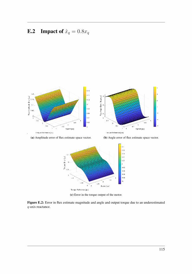
E.2 Impact of xq = 0.8xq
(a) Amplitude error of flux estimate space vector. (b) Angle error of flux estimate space vector.
(c) Error in the torque output of the motor.
Figure E.2: Error in flux estimate magnitude and angle and output torque due to an underestimatedq-axis reactance.
115

E.3 Impact of ψm = 0.8ψm
(a) Amplitude error of flux estimate space vector. (b) Angle error of flux estimate space vector.
(c) Error in the torque output of the motor.
Figure E.3: Error in flux estimate magnitude and angle and output torque due to an underestimatedpermanent magnet flux linkage.
116
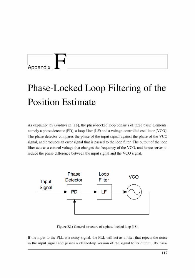
Appendix FPhase-Locked Loop Filtering of thePosition Estimate
As explained by Gardner in [18], the phase-locked loop consists of three basic elements,namely a phase detector (PD), a loop filter (LF) and a voltage-controlled oscillator (VCO).The phase detector compares the phase of the input signal against the phase of the VCOsignal, and produces an error signal that is passed to the loop filter. The output of the loopfilter acts as a control voltage that changes the frequency of the VCO, and hence serves toreduce the phase difference between the input signal and the VCO signal.
Figure F.1: General structure of a phase-locked loop [18].
If the input to the PLL is a noisy signal, the PLL will act as a filter that rejects the noisein the input signal and passes a cleaned-up version of the signal to its output. By pass-
117

ing the estimated rotor position angle through a well-designed PLL, it should be possiblethe eliminate any potential noise in θ, hence providing a better rotor position estimate.The specific PLL structure that will be used here for filtering of the position estimate ispresented in Figure F.2. Here, the loop filter is a PI controller.
Figure F.2: Structure of the PI-controller based phase-locked loop. Reproduced from [9].
Using ωn = 2πfn, the transfer function of the phase-locked loop can be written as
HPLL(s) =kpωns+ kiωn
s2 + kpωns+ kiωn(F.1)
The transfer function in Equation F.1 can be rewritten on the following general form:
HPLL(s) =2ζω0s+ ω2
0
s2 + 2ζω0s+ ω20
(F.2)
Here, ω0 is the undamped angular frequency of the system and ζ is the relative damping ra-tio. Generally, the magnitude of ω0 will determine the speed of the system response, whilethe value of ζ determines whether the system has overshoot and an oscillatory response ornot. Together, knowledge about the values of ω0 and ζ will make it possible to predict thecharacteristics of the response of the closed-loop system. By comparing Equation F.1 andEquation F.2, the PI controller gains can be expressed as functions of ω0 and ζ as shownbelow.
kp = 2ζω0
ωn(F.3)
118

ki =ω2
0
ωn(F.4)
Now, the controller can be tuned by determining which values of these parameters thatwill give the desired response. As explained in [3], a robust PLL design is achieved if thePI controller is tuned to meet the following criterion:
ζ =1√2≈ 0.707 (F.5)
Next, choosing the value of ω0 becomes a trade-off between having a fast dynamic re-sponse and narrow bandwith for good filtering performance and noise rejection.
The implementation of the PLL for rotor position filtering did not work as intended, sug-gesting that there are errors in the PLL C++ sub-routine. The PLL actually produced aposition estimate that is more polluted by noise than the original position estimate, and didas such have the opposite effect of what was intended.
119

120

Appendix GHigh-Frequency Signal Injectionfor Standstill and Low-SpeedOperation
Due to the inherent saliency of the rotor of the IPMSM, the inductances of the flux pathseen by the stator in the IPMSM will vary with the rotor position. This can be utilized byadding a high-frequency voltage signal to the voltage reference of the converter and mea-suring the corresponding response in the stator current. The ripple in the stator current dueto the high-frequency component in the stator voltage will be modulated with informationabout the rotor position, and by applying the correct demodulation technique, the positionof the rotor can be obtained [28].
The method that was attempted in this thesis is presented in [44], and is based on thework done by [52] and [28]. Here, a short introduction to the estimation scheme is pre-sented.
The square-wave voltage that will be injected in the stator is given by Equation G.1:[udhudh
]=
[uh(−1)k
0
](G.1)
In the above equation, k is used to denote the number of interrupt signals, which aregenerated at the top and bottom of the triangular PWM carrier signal. The result is that
121

a square-wave voltage with a frequency equal the switching frequency and a magnitudeequal to uh is generated and injected in the estimated d-axis, denoted as d.
The q-axis current response to the high-frequency voltage component can be approximatedusing
δiqh ≈ δiq = iq[k]− iq[k − 1] (G.2)
This approximation assumes that the current response due to the fundamental excitationis constant withing a sampling period interval. The q-axis current response can be usedto obtain an estimation of the error in the current rotor position estimate, θ, as shown inEquation G.3.
θ =xd · xq
(xq − xd) · udh[k] · ωn · Tsamp· δiq (G.3)
If this error is driven to zero using a phase-locked loop, as proposed by [44], the positionestimate coming from the saliency-tracker will correspond to the true rotor position. Thisapproach was attempted to extract the rotor position extraction, but the method was notsuccessfully implemented.
122
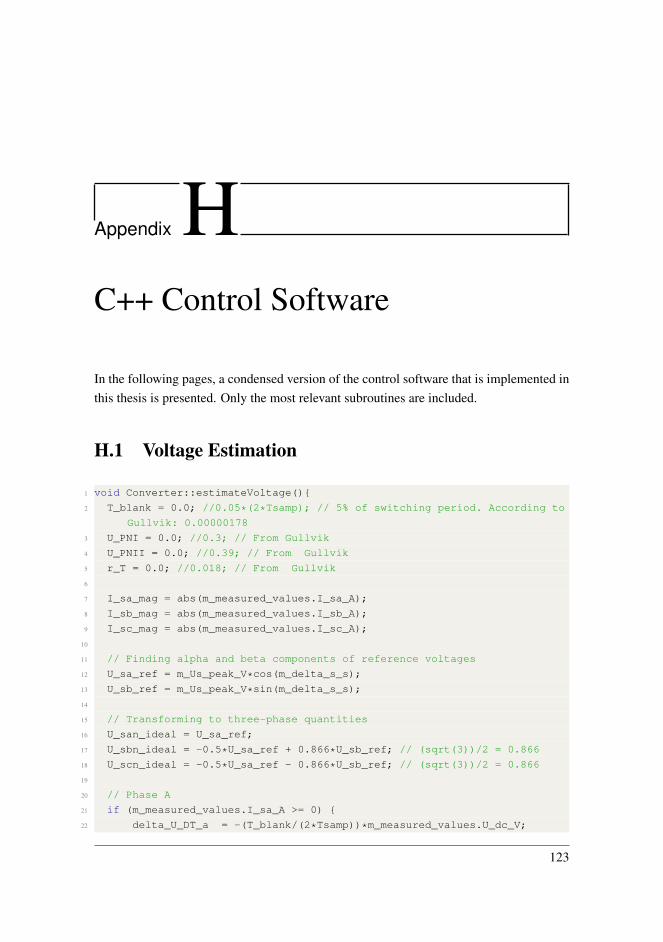
Appendix HC++ Control Software
In the following pages, a condensed version of the control software that is implemented inthis thesis is presented. Only the most relevant subroutines are included.
H.1 Voltage Estimation
1 void Converter::estimateVoltage()
2 T_blank = 0.0; //0.05*(2*Tsamp); // 5% of switching period. According to
Gullvik: 0.00000178
3 U_PNI = 0.0; //0.3; // From Gullvik
4 U_PNII = 0.0; //0.39; // From Gullvik
5 r_T = 0.0; //0.018; // From Gullvik
6
7 I_sa_mag = abs(m_measured_values.I_sa_A);
8 I_sb_mag = abs(m_measured_values.I_sb_A);
9 I_sc_mag = abs(m_measured_values.I_sc_A);
10
11 // Finding alpha and beta components of reference voltages
12 U_sa_ref = m_Us_peak_V*cos(m_delta_s_s);
13 U_sb_ref = m_Us_peak_V*sin(m_delta_s_s);
14
15 // Transforming to three-phase quantities
16 U_san_ideal = U_sa_ref;
17 U_sbn_ideal = -0.5*U_sa_ref + 0.866*U_sb_ref; // (sqrt(3))/2 = 0.866
18 U_scn_ideal = -0.5*U_sa_ref - 0.866*U_sb_ref; // (sqrt(3))/2 = 0.866
19
20 // Phase A
21 if (m_measured_values.I_sa_A >= 0)
22 delta_U_DT_a = -(T_blank/(2*Tsamp))*m_measured_values.U_dc_V;
123

23
24 else if (m_measured_values.I_sa_A < 0)
25 delta_U_DT_a = (T_blank/(2*Tsamp))*m_measured_values.U_dc_V;
26
27
28 // Phase B
29 if (m_measured_values.I_sb_A > 0)
30 delta_U_DT_b = -(T_blank/(2*Tsamp))*m_measured_values.U_dc_V;
31
32 else if (m_measured_values.I_sb_A < 0)
33 delta_U_DT_b = (T_blank/(2*Tsamp))*m_measured_values.U_dc_V;
34
35
36 // Phase C
37 if (m_measured_values.I_sc_A > 0)
38 delta_U_DT_c = -(T_blank/(2*Tsamp))*m_measured_values.U_dc_V;
39
40 else if (m_measured_values.I_sc_A < 0)
41 delta_U_DT_c = (T_blank/(2*Tsamp))*m_measured_values.U_dc_V;
42
43
44 // Output per-unit voltage estimate
45 U_sa_est = U_san_ideal + delta_U_DT_a;
46 U_sb_est = U_sbn_ideal + delta_U_DT_b;
47 U_sc_est = U_scn_ideal + delta_U_DT_c;
48
49 // Alpha-beta components of the estimated voltage
50 U_salpha_est = 0.667*U_sa_est - 0.333*U_sb_est - 0.333*U_sc_est;
51 U_sbeta_est = 0.577*U_sb_est - 0.577*U_sc_est;
Listing H.1: Stator voltage estimation code.
H.2 The Current Model
1 void MotorModel::CurrentModel()
2
3 // calculation of stator flux in rotating frame
4 m_psi_s_di = m_id*par.xd + par.psi_m;
5 m_psi_s_qi = m_iq*par.xq;
6
7 // stator flux transformation to stator frame for comparison with them
of voltage mode
8 m_psi_s_sai = m_psi_s_di*cos(theta_used) - m_psi_s_qi*sin(theta_used);
9 m_psi_s_sbi = m_psi_s_di*sin(theta_used) + m_psi_s_qi*cos(theta_used);
10
124
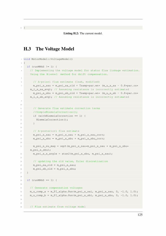
11
Listing H.2: The current model.
H.3 The Voltage Model
1 void MotorModel::VoltageModel()
2
3 if (runMRAS != 1)
4 // Implementing the voltage model for stator flux linkage estimation.
Using the Niemel method for drift compensation.
5
6 // A-priori flux estimate (Isak, modified)
7 m_psi_s_sau = m_psi_sa_old + Tsamp*par.wn* (m_u_s_sa - 0.8*par.rs*m_i_s_sa_avg); // Assuming resistance is incorrectly estimated
8 m_psi_s_sbu = m_psi_sb_old + Tsamp*par.wn* (m_u_s_sb - 0.8*par.rs*m_i_s_sb_avg); // Assuming resistance is incorrectly estimated
9
10
11 // Generate flux estimate correction terms
12 //SimpleNiemelaCorrection();
13 if (withNiemelaCorrection == 1)
14 NiemelaCorrection();
15
16
17 // A-posteriori flux estimate
18 m_psi_s_sau = m_psi_s_sau + m_psi_s_sau_corr;
19 m_psi_s_sbu = m_psi_s_sbu + m_psi_s_sbu_corr;
20
21 m_psi_s_su_mag = sqrt(m_psi_s_sau*m_psi_s_sau + m_psi_s_sbu*m_psi_s_sbu);
22 m_psi_s_s_angle = atan2(m_psi_s_sbu, m_psi_s_sau);
23
24 // updating the old value, Euler discretization
25 m_psi_sa_old = m_psi_s_sau;
26 m_psi_sb_old = m_psi_s_sbu;
27
28
29 if (runMRAS == 1)
30
31 // Generate compensation voltages
32 m_u_comp_a = m_PI_alpha.Run(m_psi_s_sai, m_psi_s_sau, 0, -1.0, 1.0);
33 m_u_comp_b = m_PI_alpha.Run(m_psi_s_sbi, m_psi_s_sbu, 0, -1.0, 1.0);
34
35
36 // Flux estimate from voltage model
125

37 m_psi_s_sau = m_psi_sa_old + Tsamp*par.wn* (m_u_s_sa - 0.8*par.rs*m_i_s_sa_avg + m_u_comp_a);
38 m_psi_s_sbu = m_psi_sb_old + Tsamp*par.wn* (m_u_s_sb - 0.8*par.rs*m_i_s_sb_avg + m_u_comp_b);
39
40 // updating the old value, Euler discretization
41 m_psi_sa_old = m_psi_s_sau;
42 m_psi_sb_old = m_psi_s_sbu;
43
Listing H.3: The voltage model.
H.4 Niemela-Correction
1 void MotorModel::NiemelaCorrection()
2
3 // Torque estimation
4 m_torque_est = (par.psi_m - (par.xq - par.xd) * m_id) * m_iq;
5
6 // Removing noise in torque estimate
7 m_torque_est = m_LPF_tau_est2.Run(m_torque_est);
8
9 // Filtering of the torque estimate
10 m_torque_est_filt = m_LPF_tau_est.Run(m_torque_est);
11
12 // Assigning value to k_T
13 m_k_T_0 = 4;
14 if (abs(k_T_0*(m_torque_est - m_torque_est_filt)) < 1)
15 m_k_T = abs(k_T_0*(m_torque_est - m_torque_est_filt));
16
17 else
18 m_k_T = 1;
19
20
21 // Assigning correction coefficient value
22 m_k_psi_0 = 0.0075;
23 m_k_psi_corr = (1 - k_T)*k_psi_0;
24
25 // Limits low-pass filter time constant to a maximum value of 1.75.
26 if ((2 / (abs(speed_est) * fn)) < 1.75 && (2 / (abs(speed_est) * fn)) >=
0)
27 m_Tfilt = 2 / (abs(speed_est) * fn);
28
29 else
30 m_Tfilt = 1.75;
31
126

32
33 // A-priori flux linkage estimate magnitude squared
34 m_psi_s_su_sqr = m_psi_s_sau*m_psi_s_sau + m_psi_s_sbu*m_psi_s_sbu;
35
36 // Modified low-pass filter
37 m_psi_s_su_sqr_filt = m_psi_s_su_sqr_filt + (Tsamp / Tfilt)*(
m_psi_s_su_sqr - m_psi_s_su_sqr_filt) +
38 k_T * (m_psi_s_su_sqr - m_psi_s_su_sqr_old);
39
40 // Updating old value of the the flux estimate squared
41 m_psi_s_su_sqr_old = m_psi_s_su_sqr;
42
43 // Error
44 m_epsilon = m_psi_s_su_sqr_filt - m_psi_s_su_sqr;
45
46 // Generating correction terms
47 m_psi_s_sau_corr = m_k_psi_corr*m_epsilon*m_psi_s_sau;
48 m_psi_s_sbu_corr = m_k_psi_corr*m_epsilon*m_psi_s_sbu;
49
50
Listing H.4: The Niemela-method for drift correction.
H.5 Position Estimation
1 void MotorModel::PositionEstimator()
2
3 // Active flux calculation
4 m_psi_Ta = m_psi_s_sau - par.xq*m_i_s_sa_avg;
5 m_psi_Tb = m_psi_s_sbu - par.xq*m_i_s_sb_avg;
6
7 // Position estimate
8 theta_est = atan2(m_psi_Tb, m_psi_Ta);
9
10 // Per-unit speed estimate
11 help1 = m_psi_Tb * m_psi_Ta_old - m_psi_Ta * m_psi_Tb_old;
12 help2 = 1/((m_psi_Ta*m_psi_Ta + m_psi_Tb*m_psi_Tb)*Tsamp*par.wn);
13 speed_est = help1*help2;
14
15 // Low-pass filtering of the speed estimate
16 m_speed_est = m_LPF_n_est.Run(speed_est);
17
18 m_psi_Ta_old = m_psi_Ta;
19 m_psi_Tb_old = m_psi_Tb;
20
Listing H.5: Rotor position estimation code.
127

NTN
UN
orw
egia
n U
nive
rsity
of S
cien
ce a
nd T
echn
olog
yFa
culty
of I
nfor
mat
ion
Tech
nolo
gy a
nd E
lect
rical
Eng
inee
ring
Dep
artm
ent o
f Ele
ctric
Pow
er E
ngin
eerin
g
Isak Nordeng Jensen
Position-Sensorless Indirect TorqueControl of Permanent MagnetSynchronous Machines
Master’s thesis in Energy and Environmental EngineeringSupervisor: Roy NilsenCo-supervisor: Alexey Matveev
June 2021
Mas
ter’s
thes
is