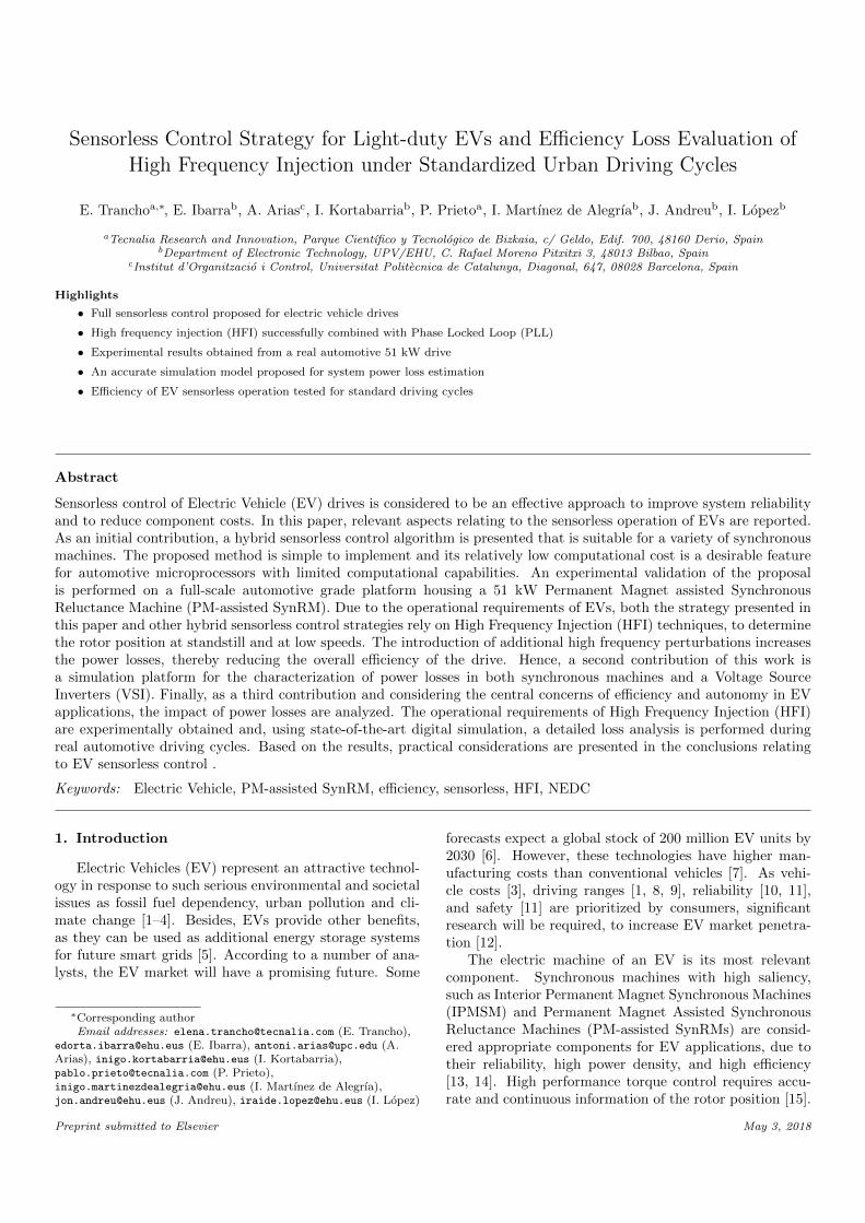
Sensorless Control Strategy for Light-duty EVs and Efficiency Loss Evaluation ofHigh Frequency Injection under Standardized Urban Driving Cycles

E. Tranchoa,∗, E. Ibarrab, A. Ariasc, I. Kortabarriab, P. Prietoa, I. Martınez de Alegrıab, J. Andreub, I. Lopezb

aTecnalia Research and Innovation, Parque Cientıfico y Tecnologico de Bizkaia, c/ Geldo, Edif. 700, 48160 Derio, SpainbDepartment of Electronic Technology, UPV/EHU, C. Rafael Moreno Pitxitxi 3, 48013 Bilbao, Spain

cInstitut d’Organitzacio i Control, Universitat Politecnica de Catalunya, Diagonal, 647, 08028 Barcelona, Spain

Highlights

• Full sensorless control proposed for electric vehicle drives

• High frequency injection (HFI) successfully combined with Phase Locked Loop (PLL)

• Experimental results obtained from a real automotive 51 kW drive

• An accurate simulation model proposed for system power loss estimation

• Efficiency of EV sensorless operation tested for standard driving cycles

Abstract

Sensorless control of Electric Vehicle (EV) drives is considered to be an effective approach to improve system reliabilityand to reduce component costs. In this paper, relevant aspects relating to the sensorless operation of EVs are reported.As an initial contribution, a hybrid sensorless control algorithm is presented that is suitable for a variety of synchronousmachines. The proposed method is simple to implement and its relatively low computational cost is a desirable featurefor automotive microprocessors with limited computational capabilities. An experimental validation of the proposalis performed on a full-scale automotive grade platform housing a 51 kW Permanent Magnet assisted SynchronousReluctance Machine (PM-assisted SynRM). Due to the operational requirements of EVs, both the strategy presented inthis paper and other hybrid sensorless control strategies rely on High Frequency Injection (HFI) techniques, to determinethe rotor position at standstill and at low speeds. The introduction of additional high frequency perturbations increasesthe power losses, thereby reducing the overall efficiency of the drive. Hence, a second contribution of this work isa simulation platform for the characterization of power losses in both synchronous machines and a Voltage SourceInverters (VSI). Finally, as a third contribution and considering the central concerns of efficiency and autonomy in EVapplications, the impact of power losses are analyzed. The operational requirements of High Frequency Injection (HFI)are experimentally obtained and, using state-of-the-art digital simulation, a detailed loss analysis is performed duringreal automotive driving cycles. Based on the results, practical considerations are presented in the conclusions relatingto EV sensorless control .

Keywords: Electric Vehicle, PM-assisted SynRM, efficiency, sensorless, HFI, NEDC

1. Introduction

Electric Vehicles (EV) represent an attractive technol-ogy in response to such serious environmental and societalissues as fossil fuel dependency, urban pollution and cli-mate change [1–4]. Besides, EVs provide other benefits,as they can be used as additional energy storage systemsfor future smart grids [5]. According to a number of ana-lysts, the EV market will have a promising future. Some

∗Corresponding authorEmail addresses: elena.trancho@tecnalia.com (E. Trancho),

edorta.ibarra@ehu.eus (E. Ibarra), antoni.arias@upc.edu (A.Arias), inigo.kortabarria@ehu.eus (I. Kortabarria),pablo.prieto@tecnalia.com (P. Prieto),inigo.martinezdealegria@ehu.eus (I. Martınez de Alegrıa),jon.andreu@ehu.eus (J. Andreu), iraide.lopez@ehu.eus (I. Lopez)

forecasts expect a global stock of 200 million EV units by2030 [6]. However, these technologies have higher man-ufacturing costs than conventional vehicles [7]. As vehi-cle costs [3], driving ranges [1, 8, 9], reliability [10, 11],and safety [11] are prioritized by consumers, significantresearch will be required, to increase EV market penetra-tion [12].

The electric machine of an EV is its most relevantcomponent. Synchronous machines with high saliency,such as Interior Permanent Magnet Synchronous Machines(IPMSM) and Permanent Magnet Assisted SynchronousReluctance Machines (PM-assisted SynRMs) are consid-ered appropriate components for EV applications, due totheir reliability, high power density, and high efficiency[13, 14]. High performance torque control requires accu-rate and continuous information of the rotor position [15].

Preprint submitted to Elsevier May 3, 2018

NomenclatureVi Voltage amplitude produced by the HFI (V)wi HF perturbation rotation speed (rad/s)fi HF perturbation rotation frequency (Hz)ωth Transition point between HFI and observer (rad/s)

eαβ Estimated back-EMF in the αβ reference frame (V)iαβ Machine voltages in the αβ reference frame (V)vαβ Machine currents in the αβ reference frame (V)Rs Stator resistance (Ω)Ls Stator inductance (H)Ld Stator inductance in the d-axis (H)Lq Stator inductance in the q-axis (H)ΨPM Permanent magnet flux linkage (Wb)ωe Electrical speed (rad/s)

ωe Estimated electrical speed (rad/s)θe Rotor electrical position (rad)

θe,PLL PLL estimated rotor electrical position (rad)

θe,HFI HFI estimated rotor electrical position (rad)

θ′e,HFI HFI estimated rotor electrical position (rad) without consid-ering polarity

∆e Angle deviation (rad)P Rotor pole-pairPN Maximum power (W)ωmax Maximum speed (rad/s)RFe Magnetic resistance (Ω)vd d-axis voltage (V)vq q-axis voltage (V)v∗d d-axis reference voltage (V)v∗q q-axis reference voltage (V)id d-axis current (A)iq q-axis current (A)i∗d d-axis reference current (A)i∗q q-axis reference current (A)Ψd d-axis flux (Wb)Ψq q-axis flux (Wb)vd,ST d-axis Super-twisting voltage (V)vq,ST q-axis Super-twisting voltage (V)vd,eq d-axis equivalent voltage (V)vq,eq q-axis equivalent voltage (V)cd d-axis equivalent voltage regulation parametercq q-axis equivalent voltage regulation parameterλd d-axis STA regulation parameterλq q-axis STA regulation parameterΩd d-axis STA regulation parameterΩq q-axis STA regulation parameterTem Electromagnetic torque (Nm)iFe,d d-axis iron loss current (A)iFe,q q-axis iron loss current (A)imag,d d-axis magnetizing current (A)imag,q q-axis magnetizing current (A)PL Machine power losses (W)PL,Cu Machine copper losses (W)PL,Fe Motor magnetic losses (W)Pcond,IGBT IGBT conduction losses (W)Tsw Switching period (s)fsw Switching frequency (Hz)

Vce Collector-emitter voltage (V)Vces Maximum blocking voltage (V)Vces Typical collector-emitter voltage (V)ic Instantaneous collector current (A)Imax Maximum collector current (A)Inom Nominal collector current (A)Tvj,IGBT IGBT junction temperature (C)Psw,IGBT IGBT switching losses (W)EON IGBT turn-on energy losses (J)EOFF IGBT turn-off energy losses (J)RG Gate resistance (Ω)CDC DC-link capacitance (F)Pcond,D Diode conduction losses (W)VF Diode forward voltage (V)iF Diode forward current (A)Psw,D Diode switching losses (W)ERR Diode recovery energy losses (J)Ploss,inv Inverter power losses (W)ωwheel Vehicle wheel speed (rad/s)ωdc Driving cycle speed (m/s)Twheel Vehicle wheel torque (Nm)rwheel Vehicle wheel radius (m)Froll Rolling resistance (N)FAero Aerodynamic resistance (N)FInertia Inertia force (N)Mcar Total vehicle mass (g)ag Gravity acceleration (m/s)µ Rolling friction coefficientρ Air density (kg/m3)Cd Drag coefficientAf Vehicle cross section (m2)Mrot Equivalent mass of rotating parts (%)acar Car acceleration (m/s2)GR Gear ratioηGR Gear ratio efficiency (%)Ttrans Transmission torque (Nm)TIdling Idling torque (Nm)PGT Idling losses (W)Ebatt Battery energy (J)Γsim Simulation factortsim Simulation completion time (s)tbehaviour Simulation time (s)Eloss,mot Motor total energy losses (J)Eloss,Cu Motor copper energy losses (J)Eloss,Fe Motor magnetic energy losses (J)Eloss,inv Inverter total energy losses (J)Eloss,condQ IGBT conduction losses (J)Eloss,swQ IGBT switching losses (J)Eloss,condD Diode conduction losses (J)Eloss,swD Diode switching losses (J)ηmot Motor efficiency (%)ηinv Inverter efficiency (%)ηdriv Drive efficiency (%)

List of AcronymsEKF Extended Kalman FilterELO Extended Luemberger ObserverEMF Electro-Motive ForceEUDC Extra Urban Driving CycleEV Electric VehicleFFT Fast Fourier TransformFPGA Field Programmable Gate ArrayFW Field WeakeningHF High FrequencyHFI High Frequency InjectionIGBT Insulated Gate Bipolar TransistorIPMSM Interior Permanent Magnet Synchronous MachineLUT Look-Up TableMRAS Model Reference Adaptive SystemMTPA Maximum Torque per Ampere

MTPV Maximum Torque per VoltNEDC New European Driving CyclePI Proportional IntegralPLL Phase Locked LoopPM Permanent MagnetRCP Rapid Control PrototypingSTA Super-Twisting AlgorithmSynRM Synchronous Reluctance MachineSMC Sliding Mode ControlSMO Sliding Mode ObserverUDC Urban Driving CycleVCT Voltage Constraint TrackingVSI Voltage Source InverterWLTP Worldwide Harmonized Light Vehicles Test

2

In general purpose drives as well as in the automotiveapplications, the most widely used rotor position sensorsare either the analog resolvers or digital (pulses) encoders.However, their use can cause not only a reduction in relia-bility, but also additional costs and an increase in the sizeof the electric drive. Therefore, there is a special interestin their elimination and this is why the so called sensor-less control techniques are still widely investigated in bothresearch institutes and industry [16, 17].

A large number of back-EMF observer-based sensorlesscontrol approaches have been reported in the scientific lit-erature. One well-known example is the Extended KalmanFilter (EKF) for rotor angle estimation that is suitable fornon-linear systems and noisy environments [18, 19]. How-ever, the major drawbacks of this method are the com-plex tuning of the covariance matrices of the EKF equa-tions and the high computational burden required duringthe state space estimation process [20]. Other alterna-tive sensorless control techniques are the Extended Luen-berger Observers (ELO) [21, 22] which, in principle, havethe same algorithm of the previously mentioned EKF, butthe single difference relies on their tuning, which is analyt-ical and based on the pole placement technique. Despitethe covariance matrices do not exist, ELOs still suffer fromhigh computational burden.

A rather different observers family are the Sliding ModeObservers (SMO) [16, 23, 24], whose main advantages aretheir robustness and low sensitivity to machine parametervariations. However, their limited sampling rate produceschattering problems, requiring additional robust strategiesto overcome rotor position estimation errors.

Finally, another approach is based on the Model Refer-ence Adaptive Systems (MRAS) [22], where the estimationis carried out by comparing a reference and an adjustablemodel. The milestone of such technique is the adaptivemechanism design with the required compromise betweenfast response and high robustness against noise and dis-turbances.

Regarding implementation aspects, automotive micro-controllers must comply with the functional safety stan-dards (ISO 26262 ASIL D and IEC 61508 SIL 3). In accor-dance to this, some well-established automotive microcon-trollers are: Freescale MPC5643L (120 MHz), MPC5675K(180 MHz), MPC5744P (200 MHz), and Texas Instru-ments TMS570 (180 MHz). Considering their limited com-putational capabilities and industrial demand for addi-tional control and monitoring functionalities, simple sen-sorless algorithms are desirable at a low computationalcost [25]. Hence, Phase Locked Loop (PLL) based estima-tors [14, 23, 26] can be considered appropriate for auto-motive applications.

All these estimation techniques fail at very low speedsor at standstill, due to the lack of back-EMF [27]. Con-sequently, they must be combined with other strategies.High Frequency Injection (HFI) techniques can be usedto obtain the rotor position at very low speeds, includingstandstill [27–31]. Taking the above into account, this pa-

per presents a hybrid sensorless control strategy that uses aPLL for rotor position estimation at medium/high speedsand an HFI technique for low speeds and standstill (fig-ure 1). These estimators have been combined with a robusttorque regulation strategy consisting of a Second OrderSliding Mode Control (SMC) algorithm for current regula-tion, complemented with a Look-up Table (LUT)/VoltageConstraint Tracking (VCT) based optimum current setpoint generator (figure 1). The proposal is implementedand experimentally validated for a 51 kW automotive gradePM-assisted SynRM drive. Additionally, the most relevantrequirements of the sensorless algorithm, i.e., the injectionvoltage magnitude, frequency and operation speed thresh-old, are all determined.

Various drawbacks should be pointed out in relation tothe use of HFI techniques [32–34]:

• A high frequency test signal is injected into the EVdrive, which produces an additional torque rippleand power losses.

• Relatively high acoustic noise is produced, as thefundamental frequency of the injected signal is withinthe audible range.

• Additional stress in the mechanical components isintroduced, due to the high frequency torque rippleeffect.

Thus, the impact of the HFI algorithm should be ana-lyzed, in order to determine its feasibility for real EV ap-plications. A second and a third contribution of this studyare, respectively, a power loss characterization model witha study of additional power losses and a study of both theefficiency and the autonomy of an EV relying on HFI. Bothcontributions provide valuable information on sensorlessoperation. A detailed simulation model was implementedin a Matlab/Simulink based RT-Lab OP4510 platform,which included the dynamics of a light-duty vehicle, powersemiconductor losses (conduction and switching losses atIGBTs and diodes), and (copper and magnetic) losses inthe electric machine. In doing so, a detailed estimationof additional HFI losses under the NEDC standardizeddriving cycle [35, 36] was conducted and their distributionbetween the drive elements was determined.

2. Proposed hybrid sensorless control strategy forsynchronous machines

2.1. Torque control loop

The torque control loop of the proposed strategy isbased on second order Sliding Mode Control (SMC) cur-rent regulators and an optimal current set-point generator(figure 1). The second order SMC technique was selectedamong other control strategies, because of its robustnessagainst parameter variations (which can be significant inautomotive synchronous machines), and because it oper-ates at a fixed switching frequency [37]. The dq reference

3

Speed

estimation

Transitio

n

Control strategy

T∗

em

ωmech

Currentsetpointgenerator

basedon

Hybrid

LUT/VCT

i∗d

i∗q

2nd order

SMC

current

control

v∗d

v∗q

dq

v∗α

v∗βαβ

HFI vector

Vαi

Vβiωthreshold

Speed threshold

vα

vβ

αβ

uvw

v∗u

v∗v

v∗w

iu

iv

iw

αβ

uvw

iα

iβαβ

dq

θe

id

iq

θe

iα,i

iβ,i

e−j2ωit

id,i

iq,i

id,if

iq,if

iα,pos

iβ,pos

ej2ωitarctan2

HFI Signal Processing

Polarity

detection

θe,HFI θ′e,HFI

θe,PLLPLL based rotor position estimation

Figure 1: General diagram of the hybrid HFI/PLL sensorless control strategy, including HF voltage vector injection, measured currentpost-processing, and the transition between both techniques.

voltages for application in the stator (figure 1) were ob-tained by applying the following control law [15]:

v∗d = vd,ST + vd,eq, (1)

v∗q = vq,ST + vq,eq. (2)

The terms vd,eq (3) and vq,eq (4) correspond to theequivalent control signals, while vd,ST and vq,ST are com-puted by applying the Super-Twisting Algorithm (STA)in (5) and (6) [38].

vd,eq = Ld

(cdeid −

−Rsid + weΨq

Ld

), (3)

vq,eq = Lq

(cqeiq −

−Rsiq − weΨd

Lq

), (4)

vd,ST = Ld

[λd|sid |1/2sgn(sid) + Ωd

∫sgn(sid)dt

], (5)

vq,ST = Lq

[λq|siq |1/2sgn(siq ) + Ωq

∫sgn(siq )dt

], (6)

where, Rs is the stator resistance; ωe is the electrical speed;id and iq are the stator currents in the synchronous refer-ence frame; Ld, Lq, Ψd and Ψq are the stator inductances

and flux linkages; eid = (i∗d − id) and eiq = (i∗q − iq) arethe current regulation errors; and, cd, cq , λd, λq, Ωd andΩq are the positive gains for tuning: sgn(sid) = sid/|sid |and sgn(siq ) = siq/|siq | and

sid = eid + cd

∫eiddt, (7)

siq = eiq + cd

∫eiqdt. (8)

Determination of the optimum current set points, i∗dand i∗q , (figure 1) throughout the whole operational rangeof the machine, i.e. Maximum Torque Per Ampere (MTPA),Field Weakening (FW), and Maximum Torque per Volt(MTPV) regions [15, 39, 40] is a complex task for ma-chines with significant saliency. For that reason, i∗d andi∗q were calculated offline and stored in LUTs. The de-termination of the set points can be done iteratively fromthe analytical solutions [39], or by using optimization algo-rithms such as the Matlab/Simulink fmincon function [41].Finally, an additional Voltage Constraint Tracking (VCT)feedback was proposed by the authors in [15], in order toimprove the robustness of the LUT-based current set pointdetermination during FW. It has since been successfullyintroduced in the proposed sensorless algorithm.

4

Figure 2: PLL-based rotor position estimation diagram.

As the control loop requires both Park transformationand anti-transformation to function, it becomes clear thatthe rotor position angle needs to be precisely determined.In this study, a hybrid rotor position estimation approachwill be introduced and described in the following section.

2.2. Medium-to-high speed sensorless strategy

A PLL-based observer (figure 2) was implemented forrotor position estimation at medium-to-high speeds, due toits simplicity and its low computational burden, which isan important feature for the integration of a sensorless con-trol algorithm in automotive grade microcontrollers withlimited computational capabilities.

Using the PLL approach, the estimated αβ componentsof the back-EMF (figure 2, back-EMF observation block)were obtained from the following conventional stator volt-age equations:

eαβ = vαβ −Rsiαβ − Lsdiαβdt

, (9)

where, iαβ and vαβ are the measured phase currents andvoltages expressed in the αβ coordinates, and Ls is thestator nominal inductance value. It is important to pointout that automotive synchronous machines are generallydesigned to obtain a significant saliency (Ld < Lq), insuch a way as to maximize the reluctant torque productionand the power density [15]. As a consequence, the statorinductance in the αβ plane depends on the rotor position,which implies a non-Linear Time-Invariant (LTI) systemwith a complex solution. A simplification of the problemis required to operate the voltage equation [42]. Hence,Ls = (Ld + Lq)/2, was considered in this study.

The following expression was obtained, by operatingthe resultant estimated back-EMF components accordingto the structure shown in figure 2 [43]:

− eαcos(θe,PLL)− eβsin(θe,PLL) = weΨPM∆e, (10)

where, we is the estimated electrical speed; θe,PLL is the

estimated electrical position; and ∆e = θe,PLL − θe is theangle deviation. The Proportional Integral (PI) controllerminimizes this error; consequently, the estimated valueθe,PLL tracks the real electrical angle.

The PLL, EKF, and SMO strategies were implementedin Matlab/Simulink and were run in real time in a single

computational node of an RT-Lab OP4510 digital simu-lator (Intel Xeon E3 4 core CPU, 3.2 GHz), in order todemonstrate the low computational burden required bythe PLL algorithm. Using the tools provided by OPAL-RTfor analysis and monitoring, it was verified that the PLLalgorithm could be executed at speeds that were 35.6 %and 13.9 % faster than the EKF and SMO, respectively.

2.3. Low speed and standstill sensorless strategy

HFI techniques (figure 1) are considered appropriate,to obtain information on rotor position at very low speedsand at standstill, due to their independence from the back-EMF [27, 28]. A rotating HF voltage vector was added tothe stator voltage references, in order to establish the rotorposition (figure 1, HFI vector block):

vi =

[vαivβi

]= Vi

[−sin(wit)cos(wit)

], (11)

where, Vi is the amplitude of the HF signal that is in-troduced; and, wi is the angular speed of rotation. Thecurrents that are measured, due to the saliency of the ma-chine, contain the rotor position at wit [27], which requiresa current signal post-processing procedure (figure 1, sig-nal processing block), details of which may be found in[27, 28, 43].

Three important requirements must be considered forproper adjustment of the HFI-based sensorless controller:

1 The magnitude of the rotating injected frequency hasto be determined. This frequency is usually set ataround 10 times higher than the fundamental fre-quency of the electrical machine and 10 times lowerthan the power converter switching frequency [33].For example, a rotation frequency of fi = 1 kHz istypically used for power converters with a switchingfrequency of around 10 kHz [27, 28].

2 The injected voltage amplitude Vi is selected in anempirical process, taking into account that an exces-sively low voltage amplitude will not produce enoughcurrent for angle estimation and that torque fluctu-ations will be greater when the value of Vi is in-creased [33].

3 A speed threshold ωth that determines the transi-tion point between the HFI and the observer needs

5

Speed [rpm]

PLLHFIPLL with HF

HysteresisHysteresis Threshold

ω1

ω2

ω3 = ωth

−ωth = −ω3

−ω2

−ω1

t [s]

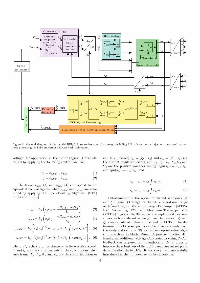
Figure 3: Conceptual operation diagram of the proposed hybrid sensorless control strategy, including transition points and operation regions.

0

π

2πθe (rad) θe,PLL

hyst. bandst [s]

π/2

3π/2

offset[0, π]

0

π

2π

θe (rad) θ′

e,HFI

θ′

e,HFI

t [s]

θe,HFI

Final HFI based estimated angle

θe,HFI

0

π

2π

t [s]

Figure 4: HFI polarity determination algorithm during transitions from PLL to HFI algorithms.

to be empirically adjusted (figure 1, speed thresholdand transition blocks) [43]. This threshold must beset at a sufficiently low value to ensure that there isenough back-EMF for correct estimation of the po-sition by the observer. In this way, the injection ofHF perturbations will be minimized.

The HFI technique can not distinguish the north andthe south poles of the magnet. It therefore generates anangle between 0 and π, leading to possible angle estimationerrors of π rad. As this error value might be unacceptable(if it reversed the polarity of the torque), the integrationof the HFI technique in the control algorithm requires aprocedure that will permit a smooth transition betweenthe HFI and the PLL algorithms. In this context, the au-thors proposed a procedure in [43], the operating principleof which is illustrated in figure 3.

The PLL estimates the angular position above the speedthreshold |ω1|, while the HFI is deactivated. When themachine reduces its speed and the operating speed is be-tween |ω1| and |ω2|, the angle obtained from the PLL is

still used by the controller, while the HFI technique is ac-tivated to start converging. An hysteresis band between|ω1| and |ω3| = |ωth| is included to change from the an-gle provided by the PLL to the one provided by the HFI,avoiding multiple changes around these speeds. The op-posite procedure is performed when accelerating.

Taking into account that HFI is restricted to low-speedoperation and standstill, the angle polarity must be checkedeach time the HFI algorithm is reactivated to restore θe,HFIproperly [27, 43]. The position polarity determinationstrategy (figure 4) is based on the information obtainedfrom the PLL-based angle estimator. The transition algo-rithm determines the required position polarity compen-sation from θe,PLL as follows:

θe,HFI =

θ′e,HFI + 0 if θe,PLL = π

2 ±Hyst,θ′e,HFI + π if θe,PLL = 3π

2 ±Hyst,(12)

where, Hyst is an hysteresis band that is included to avoiderrors in polarity determination, due to possible angle off-sets between both estimators. In this way, a reliable change

6

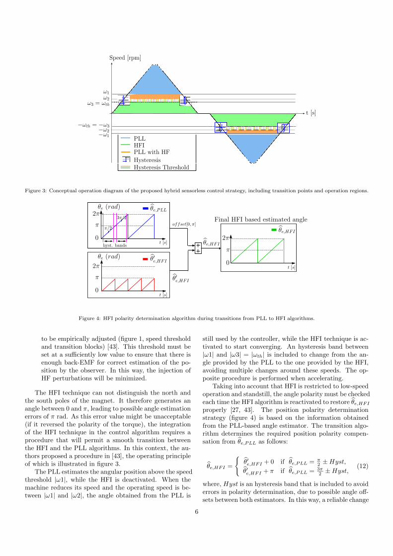
Figure 5: Automotive grade testbench.

Table 1: Most significant parameters of the PM-assisted SynRMmachine.

Item Symbol Value UnitsMaximum power PN 51 kWMaximum speed wmax 12000 rpm

Machine Pole Pairs P 3 -Stator Resistance Rs 0.012 Ω

d-axis nominal inductance Ld 0.7e−3 Hq-axis nominal inductance Lq 1.7e−3 H

Permanent Magnet Flux linkage ΨPM 0.38 WbMagnetic Resistance RFe 20 Ω

is assured.

3. Experimental validation

3.1. Experimental platform description

The proposed hybrid sensorless strategy was validatedin an automotive grade test bench (figure 5), composed ofthe following main components:

• An induction load machine of 8000 rpm and 157 kW,which emulates the behavior (speed and torque char-acteristics) of an electric vehicle.

• A 1:1.8 Gearbox between the load and test machine.

• A dSPACE Rapid Control Prototyping (RCP) digi-tal device, equipped with a DS1006 DSP board andan AC Motor Control Solutions board.

• An industrial power converter (Semikron IGD-1-424-P1N4-DL-FA) with a nominal power of 140 kW anda maximum switching frequency of 25 kHz.

• A torquimeter (HBM T40B).

The hybrid sensorless strategy was validated in a 51 kWPM-assisted SynRM, the most important nominal param-eters of which are shown in table 1.

3.2. Determination of HFI requirements and experimentalvalidation of the proposed sensorless control algorithm

At a first stage, the most significant HFI parameterswere set using a trial and error procedure, where the min-imum Vi and ωth values that ensure a robust sensorless

operation were determined. In this particular applica-tion, Vi was set at 60 V (18.75 % of the available DCbus) at a rotating frequency of 1 kHz and with a speedthreshold |ωth| = |ω3| of 800 rpm (6.67 % of the SynRMspeed range). Additionally, the values |ω1| = 1000 rpm,|ω2| = 975 rpm and Hyst = 1.5 rad were considered forthe parametrization of the transition algorithm.

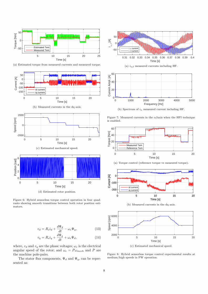
Figure 6 shows the results of the proposed hybrid sen-sorless strategy operating in both motor and generatormode, including positive speed, speed reversal and stand-still operation. The estimated torque from measured cur-rents vs the measured torque (figure 6(a)), the measuredcurrents (figure 6(b)), the estimated speed (figure 6(c)),and the estimated rotor position (figure 6(d)) all showedthe satisfactory performance of the sensorless control al-gorithm. As can be seen from the figures, relatively highelectromagnetic torque and current ripple values were in-troduced when the HFI technique was activated. Notethat the torquimeter cannot measure the high frequencytorque component. Figure 7 shows a detail of the currentsmeasured in the αβ plane (figure 7 (a)), including a FastFourier Transform (FFT) of α, from which the HF com-ponent at the rotating frequency fi = 1 kHz is obtained(figure 7 (b)). Finally, figure 8 shows sensorless torquecontrol operation above the base speed, confirming satis-factory torque regulation during field weakening.

Thus, the HFI method ensures correct rotor positionand speed estimation both at low speeds and at standstill,at the cost of increasing the drive losses, as shown in fig-ures 6(a) and 6(b). Its impact on drive performance canbe minimized by means of a correct adjustment of Vi andwth, which are highly influenced by the electrical param-eters of the machine. If the electric machine is designedwith a higher permanent magnet flux (ΨPM ), the observeroperation range could be extended, or in other words, thespeed threshold, wth, could be shortened: in addition, thehigher the saliency of the machine, the lower the requiredvalue of Vi.

In the following sections, the impact of the HFI sen-sorless technique on the power losses and the efficiency ofa light-duty EV drive will be analyzed under the standardNEDC driving cycle. As a first step, an accurate motorand inverter loss model, including driving cycle simulationcapability, was developed to quantify the aforementionedparameters. Focusing on the experimentally determinedHFI parameters, this study was extended to various com-binations of Vi and wth, in order to arrive at conclusionson the desired features of a sensorless drive design.

4. Power loss characterization in EV drive systems

4.1. Synchronous machine electrical model

A synchronous machine can be mathematically repre-sented using the synchronous dq reference frame, where thed-axis is in the direction of permanent magnet flux. Ne-glecting the iron losses, the equations for stator voltagesin the dq reference frame are [44]:

7

Time [s]5 10 15 20 25

Tor

que

[Nm

]

-50

0

50

Estimated TemMeasured Tem

(a) Estimated torque from measured currents and measured torque.

Time [s]0 5 10 15 20

Cur

rent

[A]

-150

-100

-50

0

50

id currentiq current

(b) Measured currents in the dq axis.

Time [s]0 5 10 15 20

Spe

ed [r

pm]

-2000

0

2000

(c) Estimated mechanical speed.

Time [s]0 5 10 15 20

Pos

ition

[rad

]

0

2

4

6

(d) Estimated rotor position.

Figure 6: Hybrid sensorless torque control operation in four quad-rants showing smooth transitions between both rotor position esti-mators.

vd = Rsid +dΨd

dt− ωeΨq, (13)

vq = Rsiq +dΨq

dt+ ωeΨd, (14)

where, vd and vq are the phase voltages; ωe is the electricalangular speed of the rotor; and ωe = Pωmech and P arethe machine pole-pairs.

The stator flux components, Ψd and Ψq, can be repre-sented as:

Time [s]0.31 0.32 0.33 0.34 0.35 0.36 0.37 0.38 0.39 0.4

i ,,-

[A]

-50

0

50

i , currenti - current

(a) iαβ measured currents including HF.

Frequency [Hz]0 1000 2000 3000 4000 5000

Cur

rent

Am

pl. [

A]

0

20

40

60

(b) Spectrum of iα measured current including HF.

Figure 7: Measured currents in the αβaxis when the HFI techniqueis enabled.

Time [s]0 5 10 15 20

Tor

que

[Nm

]

0

20

40

60

Measured TemReference Tem

(a) Torque control (reference torque vs measured torque).

Time [s]0 5 10 15 20

Cur

rent

[A]

-200

-100

0

iq currentid current

Time [s]0 5 10 15 20

Cur

rent

[A]

-200

-100

0

id currentiq current

(b) Measured currents in the dq axis.

Time [s]0 5 10 15 20

Spe

ed [r

pm]

2000

4000

6000

(c) Estimated mechanical speed.

Figure 8: Hybrid sensorless torque control experimental results atmedium/high speeds in FW operation.

8

vd RFe,d ωeΨq

LdRdid imag,d

iFe,d

vq RFe,q ωeΨd

LqRqiq imag,q

iFe,q

Figure 9: Equivalent machine stator voltage circuits.

Ψd = Ldid + ΨPM , (15)

Ψq = Lqiq, (16)

where ΨPM is the flux linkage produced by the perma-nent magnets. The electromagnetic torque is given by thefollowing expression:

Tem =3

2PΨdiq −Ψqid. (17)

4.2. Synchronous machine model including power losses

Motor electrical power losses consist of iron and copperlosses [45, 46]. Fictive resistors, RFe,d, and, RFe,q, wereadded to the equivalent stator voltage circuits, in order torepresent the impact of the iron losses produced by thefundamental stator electrical frequency (figure 9):

iFe,d = − ωeΨq

RFe,d, (18)

iFe,q =ωeΨd

RFe,q, (19)

where,

imag,d = id − iFe,d, (20)

imag,q = iq − iFe,q, (21)

In which, iFe,d and iFe,q are the iron loss currents; and,imag,d and imag,q are the magnetizing currents responsiblefor torque production. Taking into account the iron lossesin the electromagnetic torque equation, phase currents in(17) must be replaced by (20) and (21), as follows:

Tem =3

2P (Ψdimag,q −Ψqimag,d), (22)

Tem =3

2P

[Ψd

(iq −

ωeΨd

RFe

)−Ψq

(id +

ωeΨq

RFe

)]. (23)

In contrast, the total power losses of a motor consistingof its iron and copper losses can be represented as [47, 48]:

PL = PL,Cu + PL,Fe =3

2

[Rs(i

2d + i2q) +

ω2e

RFe(Ψ2

d + Ψ2q)

].

(24)When HFI is introduced, the additional current rip-

ple produced by the injection and the following iron lossterm must also be included (24) to represent the additionallosses:

PHFIFe =3

2

ω2i

RHFIFe

(Ψ2d,HFI + Ψ2

q,HFI), (25)

where, RHFIFe is the magnetic resistance at ωi; and, Ψd,HFI

and Ψq,HFI are the magnetic fluxes produced by the HFcomponent on the d- and q-axes, respectively.

4.3. Voltage Source Inverter power losses

Calculation of the conduction and the switching lossesof each IGBT and diode [49] are required, in order to deter-mine the power losses of the Voltage Source Inverter (VSI)responsible for synthesizing the electric machine phase volt-ages. Considering a given gate resistance, Rg, and a DClink voltage, VDC , the average conduction losses of a singleIGBT over a modulation period can be expressed as:

Pcond,IGBT =1

Tsw

∫ Tsw

0

Vce(ic, Tvj,IGBT )ic(t)dt, (26)

where, Vce(ic, Tvj,IGBT ) is the collector-emitter voltage drop;ic(t) is the instantaneous current circulating through thesemiconductor; Tsw is the modulation period; and, Tvj,IGBTis the virtual junction temperature of the IGBT. The switch-ing losses of the IGBT during a modulation period can beexpressed as:

Psw,IGBT =1

Tsw[EON (ic) + EOFF (ic)], (27)

where, EON (ic) and EOFF (ic) are the instantaneous en-ergy losses produced in the ON and OFF switching in-stants (figure 10), respectively. Similarly, the conductionand switching losses of the anti-parallel diode during amodulation period can be expressed as:

Pcond,D =1

Tsw

∫ Tsw

0

VF (iF , Tvj,D)iF (t)dt, (28)

Psw,D =1

TswERR(iF ), (29)

where, VF (iF , Tvj,D) is the diode forward voltage; iF (t) isthe instantaneous current circulating through the diode;Tvj,D is the virtual junction temperature of the diode; and,ERR(iF ) is the reverse recovery energy loss (figure 10).

Finally, the total instantaneous inverter losses can beexpressed as:

9

Current [A]0 50 100 150 200

Elo

ss [J

]

0

0.01

0.02

EON

EOFF

EREC

Figure 10: EON , EOFF and ERR energy losses vs current for thediscrete IR AUIRGPS4067D1 IGBT (at 175C and VCE = 400 V).

Table 2: Most relevant parameters of the simulated power electronicssystem including IR AUIRGPS4067D1 devices.

IGBT and diode parametersParameter Symbol Value Units

Number of parallel devices - 3 -Maximum current per switch Ic,max 160 ANominal current per switch Ic,nom 10 AMaximum blocking voltage Vces 600 V

Typical collector-emitter voltage Vce,ON 1.7 VTypical turn-on switching loss EON 8.2 mJTypical turn-off switching loss EOFF 2.9 mJTypical diode reverse recovery EREC 2.4 mJ

Junction temperature Tvj 85 CPower converter parameters

DC link capacitance CDC 3 mFSwitching frequency fsw 10 kHz

Battery voltage Vbatt 320 VGate resistance (ON and OFF) RG 5 Ω

Ploss,inv =

N∑i=0

(Pcond,IGBTi + Psw,IGBTi)+

+

M∑j=0

(Pcond,Dj + Psw,Dj ), (30)

where, N and M are the number of IGBTs and diodesthat constitute the VSI, respectively.

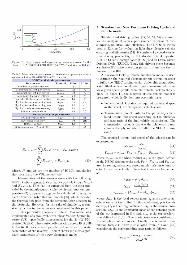
Determination of the losses is done with the followingratios: Vce(ic, Tvj,IGBT ), EON (ic), EOFF (ic), VF (iF , Tvj,D),and ERR(iF ). They can be extracted from the data pro-vided by the manufacturer, while the virtual junction tem-peratures Tvj,IGBT and Tvj,D can be calculated from equiv-alent Cauer or Foster thermal models [50], which considerthe thermal flow path from the semiconductor junction tothe heatsink. However, for the sake of simplicity, a con-stant junction temperature was considered in this paper.

In this particular analysis, a detailed loss model wasimplemented of a two-level/three-phase Voltage Source In-verter (VSI) specifically dimensioned for the 51 kW PM-assisted SynRM. Three automotive grade discrete IR AUIR-GPS4067D1 devices were parallelized, in order to createeach switch of the inverter. Table 2 shows the most signif-icant parameters of the power electronics model.

5. Standardized New European Driving Cycle andvehicle model

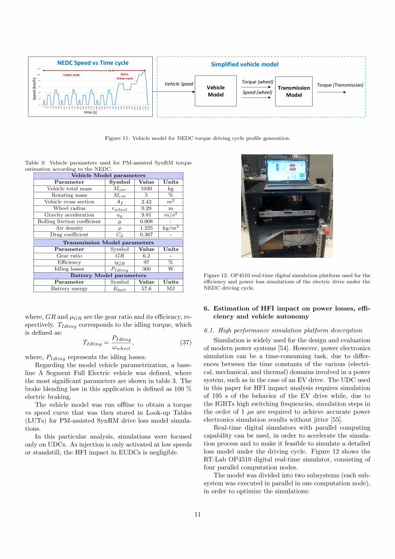
Standardized driving cycles [35, 36, 51, 52] are usefulfor the analysis of vehicle performance in terms of con-sumption, pollution, and efficiency. The NEDC is widelyused in Europe for evaluating light-duty electric vehiclesensuring realistic results [53]. It consists of a speed-versus-time driving profile (figure 11), divided into 4 repeatedECE-15 Urban Driving Cycles (UDC) and an Extra-UrbanDriving Cycle (EUDC). Thus, this driving cycle becomesa suitable EV drive operation pattern to analyze the in-fluence of the HFI.

A backward looking vehicle simulation model is usedto estimate the required electromagnetic torque, in orderto fulfill the NEDC driving cycle. Under this assumption,a simplified vehicle model determines the estimated torquefor a given speed profile, from the vehicle back to the en-gine. In figure 11, the diagram of this vehicle model ispresented, which is divided into two main tasks:

• Vehicle model: Obtains the required torque and speedin the wheel, for the specific vehicle class.

• Transmission model: Adapts the previously calcu-lated torque and speed according to the efficiencyand gear ratio of the final vehicle transmission. Thetransmission torque is the one that the electric ma-chine will apply, in order to fulfill the NEDC drivingcycle.

The required torque and speed of the wheels can beexpressed as:

ωwheel =ωdcrwheel

, (31)

Twheel = rwheel(FRoll + FAero + FInertia), (32)

where, rwheel is the wheel radius; ωdc is the speed definedin the NEDC driving cycle; and, FRoll, FAero, and FInertiaare the rolling resistance, aerodynamic resistance, and in-ertia forces, respectively. These last three can be definedas:

FRoll = µagMcar, (33)

FAero =ρω2

dcCdAf2

, (34)

FInertia = Mcar(1 +Mrot)acar, (35)

where, Mcar is the total vehicle mass; ag is the gravity ac-celeration; µ is the rolling friction coefficient; ρ is the airdensity; Cd is the drag coefficient; Af is the vehicle crosssection; Mrot is the equivalent mass of the rotating partsof the car (expressed in %); and, acar is the car accelera-tion defined as dv/dt. The grade force was considered inthis simplified vehicle model. Finally, the required trans-mission torque is directly calculated from (31) and (32)considering the corresponding gear ratio as follows:

Ttrans =TIdling + Twheel

µGRGR, (36)

10

Vehicle Model

Transmission Model

Simplified vehicle model

Torque (wheel)

Speed (wheel)

Torque (Transmission)Vehicle Speed

NEDC Speed vs Time cycle

time [s]

Spe

ed [

km/h

]

Figure 11: Vehicle model for NEDC torque driving cycle profile generation.

Table 3: Vehicle parameters used for PM-assisted SynRM torqueestimation according to the NEDC.

Vehicle Model parametersParameter Symbol Value Units

Vehicle total mass Mcar 1030 kgRotating mass Mrot 5 %

Vehicle cross section Af 2.42 m2

Wheel radius rwheel 0.29 mGravity acceleration ag 9.81 m/s2

Rolling friction coefficient µ 0.008 -Air density ρ 1.225 kg/m3

Drag coefficient Cd 0.367 -

Transmission Model parametersParameter Symbol Value UnitsGear ratio GR 6.2 -Efficiency ηGR 97 %

Idling losses PIdling 300 WBattery Model parameters

Parameter Symbol Value UnitsBattery energy Ebatt 57.6 MJ

where, GR and µGR are the gear ratio and its efficiency, re-spectively. TIdling corresponds to the idling torque, whichis defined as:

TIdling =PIdlingωwheel

, (37)

where, PIdling represents the idling losses.Regarding the model vehicle parametrization, a base-

line A Segment Full Electric vehicle was defined, wherethe most significant parameters are shown in table 3. Thebrake blending law in this application is defined as 100 %electric braking.

The vehicle model was run offline to obtain a torquevs speed curve that was then stored in Look-up Tables(LUTs) for PM-assisted SynRM drive loss model simula-tions.

In this particular analysis, simulations were focusedonly on UDCs. As injection is only activated at low speedsor standstill, the HFI impact in EUDCs is negligible.

Figure 12: OP4510 real-time digital simulation platform used for theefficiency and power loss simulations of the electric drive under theNEDC driving cycle.

6. Estimation of HFI impact on power losses, effi-ciency and vehicle autonomy

6.1. High performance simulation platform description

Simulation is widely used for the design and evaluationof modern power systems [54]. However, power electronicssimulation can be a time-consuming task, due to differ-ences between the time constants of the various (electri-cal, mechanical, and thermal) domains involved in a powersystem, such as in the case of an EV drive. The UDC usedin this paper for HFI impact analysis requires simulationof 195 s of the behavior of the EV drive while, due tothe IGBTs high switching frequencies, simulation steps inthe order of 1 µs are required to achieve accurate powerelectronics simulation results without jitter [55].

Real-time digital simulators with parallel computingcapability can be used, in order to accelerate the simula-tion process and to make it feasible to simulate a detailedloss model under the driving cycle. Figure 12 shows theRT-Lab OP4510 digital real-time simulator, consisting offour parallel computation nodes.

The model was divided into two subsystems (each sub-system was executed in parallel in one computation node),in order to optimize the simulations:

11

• Master subsystem: includes the control algorithmsand the previously detailed HFI strategy, data log-ging, and energy and efficiency calculation blocks.

• Slave subsystem: includes the electric machine,the inverter loss models, and the instantaneous powercalculations for both the electric machine and the in-verter.

With this configuration, on average, it is possible tosimulate the whole NEDC cycle with a simulation step of1 µs in 63 minutes, approximately, leading to the followingsimulation factor:

Γsim =tsim

tbehaviour= 19.5, (38)

where, Γsim = 1 corresponds to a real-time simulation;and, Γsim > 1 corresponds to a slower than real-time sim-ulation.

6.2. UDC simulation results

The main objective of this simulation study is to quan-tify the additional power losses introduced by HFI-basedsensorless strategies. This approach allows us to deter-mine whether it is possible to use the proposed algorithm(or other similar approaches) continuously in the automo-tive context. In this context, the sensorless operation wasconsidered ideal (perfect angle tracking), and only the per-turbation injection below the speed threshold wth was con-sidered. For this analysis, the PM-assisted SynRM drivewas connected to a 16 kWh battery. An ideal batterymodel was implemented. The loss and efficiency analysisfor each case study was performed by calculating the lossenergies produced during a single UDC, and extrapolatedfor hypothetical continuous urban driving of the light-dutyelectric vehicle.

Figure 13 shows the torque and speed profiles obtainedin simulation under the UDC when no HFI is injected. Ad-ditionally, figure 14 shows the performance of stator cur-rent regulation under the UDC. As can be seen from figures13 and 14, the performance of the control algorithm wasas desired, as the electromagnetic torque of the machinefollowed the reference torque set point. In addition, figure15(a) shows the additional current ripples introduced whenthe high frequency perturbation was applied for Vi = 60 Vand ωth = 800 rpm. Note that the apparent HFI ripplebehavior shown in figure 15(a) (at the beginning of thesimulation) was a consequence of the aliasing process thatoccurred as control samples were captured at a low sam-pling ratio.

It was confirmed from the results of the simulation thatsmall variations in the determination of an optimal ωthunder real driving conditions can be neglected. The vehicleaccelerates from standstill to speeds higher than ωth withina few seconds, within a limited operational interval. Forexample, a theoretical improvement in autonomy in theorder of 0.01 % was verified by simulation for Vi = 60 V

time [s]0 20 40 60 80 100 120 140 160 180

Tor

que

[Nm

]

-50

0

50

100

time [s]0 20 40 60 80 100 120 140 160 180

Spe

ed [r

pm]

0

1000

2000

3000

Figure 13: Torque and speed profiles obtained for a single UDC whenno HFI is carried out.

when ωth was reduced from 800 rpm to 400 rpm. Hence,further simulations were focused on the contribution of Vito drive losses and efficiency.

Table 4 shows the battery energy consumption (Ebatt),motor and inverter energy losses (Eloss,mot and Eloss,inv),and motor, inverter, and drive efficiencies (ηmot, ηinv andηdriv), theoretical autonomy and autonomy reduction re-sults for all of the cases under study. As can be seen fromthese results, an autonomy reduction of 0.74 % was pre-dicted by simulation when the HFI operation conditionsspecified by the experimental results, i.e., Vi = 60 V andωth = 800 rpm, were applied. However, a significant powerloss reduction was achieved when minimizing HFI (0.21 %of autonomy reduction for Vi = 20). Similarly, an evalua-tion of the power losses caused by the HFI was evaluatedunder the Urban Dynamometer Driving Schedule (UDDS),where an autonomy reduction of 0.26 % was obtained forVi = 60. The impact of the additional HFI losses in thisdriving cycle was lower than in the UDC, as the injectiontime during UDDS is significantly more limited.

HFI sensorless techniques have generally been consid-ered as a source of additional system losses [32–34]. How-ever, this work has demonstrated that, considering an ef-ficient electric machine design that provides reduced ironlosses, the efficiency reduction in the electric machine dueto HFI is very low. Additionally, if a start/stop controlstrategy is included in the EV control unit which deacti-vates the HFI when the drive is at standstill, power lossesare greatly minimized (table 4). Figure 15 (b) shows howthe current ripple due to HFI is reduced using this ap-proach. Additional power losses are minimized using thestart/stop control strategy, which obtain a negligible re-duction of autonomy of around 0.03 %. Thus, followingthese guidelines, an HFI based sensorless strategy is, fromthe point of view of efficiency, feasible for an EV applica-

12

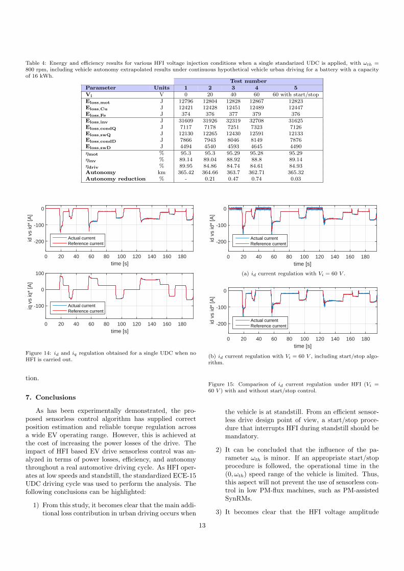
Table 4: Energy and efficiency results for various HFI voltage injection conditions when a single standarized UDC is applied, with ωth =800 rpm, including vehicle autonomy extrapolated results under continuous hypothetical vehicle urban driving for a battery with a capacityof 16 kWh.

Test numberParameter Units 1 2 3 4 5Vi V 0 20 40 60 60 with start/stopEloss,mot J 12796 12804 12828 12867 12823Eloss,Cu J 12421 12428 12451 12489 12447Eloss,Fe J 374 376 377 379 376Eloss,inv J 31609 31926 32319 32708 31625Eloss,condQ J 7117 7178 7251 7323 7126Eloss,swQ J 12130 12265 12430 12591 12133Eloss,condD J 7866 7943 8046 8149 7876Eloss,swD J 4494 4540 4593 4645 4490ηmot % 95.3 95.3 95.29 95.28 95.29ηinv % 89.14 89.04 88.92 88.8 89.14ηdriv % 89.95 84.86 84.74 84.61 84.93Autonomy km 365.42 364.66 363.7 362.71 365.32Autonomy reduction % - 0.21 0.47 0.74 0.03

time [s]0 20 40 60 80 100 120 140 160 180

id v

s id

* [A

]

-200

-100

0

Actual currentReference current

time [s]0 20 40 60 80 100 120 140 160 180

iq v

s iq

* [A

]

-100

0

100

Actual currentReference current

Figure 14: id and iq regulation obtained for a single UDC when noHFI is carried out.

tion.

7. Conclusions

As has been experimentally demonstrated, the pro-posed sensorless control algorithm has supplied correctposition estimation and reliable torque regulation acrossa wide EV operating range. However, this is achieved atthe cost of increasing the power losses of the drive. Theimpact of HFI based EV drive sensorless control was an-alyzed in terms of power losses, efficiency, and autonomythroughout a real automotive driving cycle. As HFI oper-ates at low speeds and standstill, the standardized ECE-15UDC driving cycle was used to perform the analysis. Thefollowing conclusions can be highlighted:

1) From this study, it becomes clear that the main addi-tional loss contribution in urban driving occurs when

time [s]0 20 40 60 80 100 120 140 160 180

id v

s id

* [A

]

-200

-100

0

Actual currentReference current

(a) id current regulation with Vi = 60 V .

time [s]0 20 40 60 80 100 120 140 160 180

id v

s id

* [A

]

-200

-100

0

Actual currentReference current

(b) id current regulation with Vi = 60 V , including start/stop algo-rithm.

Figure 15: Comparison of id current regulation under HFI (Vi =60 V ) with and without start/stop control.

the vehicle is at standstill. From an efficient sensor-less drive design point of view, a start/stop proce-dure that interrupts HFI during standstill should bemandatory.

2) It can be concluded that the influence of the pa-rameter ωth is minor. If an appropriate start/stopprocedure is followed, the operational time in the(0, ωth) speed range of the vehicle is limited. Thus,this aspect will not prevent the use of sensorless con-trol in low PM-flux machines, such as PM-assistedSynRMs.

3) It becomes clear that the HFI voltage amplitude

13

must be minimized, in order to reduce the impact ofthe sensorless strategy in the drive efficiency and ve-hicle autonomy. Thus, machines with high saliencythat facilitate HFI sensors are preferred. However,the experimental results have shown that relativelyhigh injection voltage levels are required in some realapplications, due to the operation of the drives innoisy environments.

4) As it is a high frequency perturbation, its impacton the core losses can be great. For sensorless EVdrives, special attention should be lent to design as-pects of the electric machine, in order to minimizethe aforementioned losses.

The simulation and experimental results obtained forthe proposed sensorless control approach are promising.However, extensive tests (including tests in real EV) willhave to be conducted to move towards any industrializa-tion of the proposed solution. Additionally, the impactof the HFI on the mechanical elements of the powertrain(possible degradation of the mechanical elements) shouldalso be studied. Likewise, in the interests of driver andpassenger comfort, the additional acoustic noise producedby the HFI should be quantified and considered in the ve-hicle design. This additional noise, if significant outsidethe vehicle, could be exploited to improve the safety ofpedestrians.

Acknowledgements

The present work has been supported by the Gov-ernment of Spain through Projects DPI2017-85404-P andDPI2014-53685-C2-2-R of the Ministerio de Economıa yCompetitividad, through Project 2017 SGR 872 of the Gen-eralitat de Catalunya, and through Project KT4eTRANS(KK-2015/00047 and KK-2016/00061) and GANICS (KK-2017/00050), within the ELKARTEK program of the Gov-ernment of the Basque Country.

This research has been conducted within the Researchand Education Unit UFI11/16 of the UPV/EHU and hasreceived funding from the Basque Government directedat research groups in the Basque government through theDepartment of Education, Linguistic Policy and Culture.

Bibliography

[1] C. Capasso, O. Veneri, Experimental analysis on the perfor-mance of lithium based batteries for road full electric and hybridvehicles, Applied Energy 136 (2014) 921–930.

[2] Z. Wei, J. Xu, D. Halim, HEV power management control strat-egy for urban driving, Applied Energy 194 (2017) 705–714.

[3] J. Gonzalez Palencia, Y. Otsuka, M. Araki, S. Shiga, Scenarioanalysis of lightweight and electric-drive vehicle market pene-tration in the long-term and impact on the light-duty vehiclefleet, Applied Energy 204 (2017) 1444–1462.

[4] E. Moreira, A. Rodrigues, J. Sodre, Analysis of CO2 emissionsand techno-economic feasibility of an electric commercial vehi-cle, Applied Energy 193 (2017) 297–307.

[5] Y. Wang, W. Shi, B. Wang, C. Chu, R. Gadh, Optimal oper-ation of stationary and mobile batteries in distribution grids,Applied Energy 190 (2017) 1289–1301.

[6] Global EV outlook, beyond on million electric cars, Tech. rep.,International Energy Agency (2017).

[7] K. Palmer, J. Tate, Z. Wadud, J. Nellthorp, Total cost of own-ership and market share for hybrid and electric vehicles in theUK, US and Japan, Applied Energy 209 (2018) 108–119.

[8] X. Ding, H. Guo, R. Xioung, F. Chen, D. Zhang, C. Gerada, Anew strategy of efficiency enhancement for traction systems inelectric vehicles, Applied Energy 205 (2017) 880–891.

[9] O. Veneri, C. Capasso, E. Patalano, Experimental study onthe performance of a ZEBRA battery based propulsion systemfor urban commercial vehicles, Applied Energy 185 (2) (2017)2005–2018.

[10] S. Chakrabortya, E. Kellerb, A. Rayb, J. Mayerb, Detectionand estimation of demagnetization faults in permanent magnetsynchronous motors, Electric Power System Research 96 (2013)225–236.

[11] S. Rezvanizaniani, Z. Liu, Y. Chen, J. Lee, Review and recentadvances in battery health monitoring and prognostics tech-nologies for electric vehicle (EV) safety and mobility, Journal ofPower Sources 256 (2014) 110–124.

[12] J. Miller, D. Howell, The EV everywhere grand challenge, in:Proc. of the EVS27 International Battery, Hybrid and Fuel CellElectric Vehicle Symposium, 2013, pp. 1–6.

[13] T. Finken, M. Hombitzer, K. Hameyer, Study and comparisonof several permanent-magnet excited rotor types regarding theirapplicability in electric vehicles, in: Proc. of Emobility - Elec-trical Power Train Conference, 2010, pp. 1–7.

[14] C. Olivieri, M. Tursini, A novel PLL scheme for a sensorlessPMSM drive overcoming common speed reversal problems, in:Proc. of the International Symposium on Power Electronics,Electrical Drives, Automation and Motion, 2012, pp. 1051–1056.

[15] E. Trancho, E. Ibarra, A. Arias, I. Kortabarria, J. Jurgens,L. Marengo, A. Fricasse, J. Gragger, PM-assisted synchronousreluctance machine flux weakening control for EV and HEVapplications, IEEE Transactions on Industrial Electronics 65 (4)(2018) 2986–2995.

[16] Z. Qiao, T. Shi, Y. Wang, Y. Yan, C. Xia, X. He, New sliding-mode observer for position sensorless control of permanent-magnet synchronous motor, IEEE Transactions on IndustrialElectronics 60 (2) (2013) 710–719.

[17] Y. Lee, Y. Kwon, S. Sul, Comparison of rotor position estima-tion performance in fundamental-model-based sensorless controlof PMSM, in: Proc. of the IEEE Energy Conversion Congressand Exposition (ECCE), 2015, pp. 5624–5633.

[18] S. Bolognani, L. Tubiana, M. Zigliotto, Extended Kalman fil-ter tuning in sensorless PMSM drives, IEEE Transactions onIndustry Applications 39 (6) (2003) 1741–1747.

[19] D. Janiszewski, Extended Kalman Filter Based Speed Sensor-less PMSM Control with Load Reconstruction, INTECH, 2010,Kalman Filter, Chap. 8, pp. 145-160.

[20] M. Huang, A. Moses, F. Anayi, The comparison of sensorlessestimation techniques for PMSM between Extended KalmanFilter and Flux-linkage Observer, in: Proc. of the Applied PowerElectronics Conference and Exposition (APEC), 2006, pp. 654–659.

[21] N. Henwood, J. Malaiz, L. Plary, A robust nonlinear LuenbergerObserver for the sensorless control of SM-PMSM: Rotor positionand magnets flux estimation, in: Proc. of the IEEE IndustrialElectronics Society Conference (IECON), 2012, pp. 1625–1630.

[22] M. Jouili, K. Jarray, Y. Koubaa, M. Boussak, A LuenbergerState Observer for simultaneous estimation of speed and rotorresistance in sensorless indirect stator flux orientation controlof induction motor drive, in: Proc. of the International Con-ference on Sciences and Techniques of Automatic Control andComputer Engineering (STA), 2011, pp. 898–904.

[23] R. Li, G. Zhao, Position sensorless control for PMSM usingsliding mode observer and phase-locked loop, in: Proc. of the

14

Power Electronics and Motion Control Conference (IPEMC),2009, pp. 1867–1870.

[24] H. Kim, J. Son, J. Lee, A high-speed sliding-mode observer forthe sensorless speed control of a PMSM, IEEE Transactions onIndustrial Electronics 58 (9) (2011) 4069–4077.

[25] E. Dehghan-Azad, S. Gadoue, D. Atkinson, H. Slater, P. Bar-rass, F. Blaabjerg, Sensorless control of IM for limp-home modeEV applications, IEEE Transactions on Power Electronics 32 (9)(2017) 7140–7150.

[26] G. El-Murr, D. Giaouris, J. Finch, Universal PLL strategy forsensorless speed and position estimation of PMSM, in: Proc. ofthe IEEE Industrial and Information Systems Conference, 2008,pp. 1–6.

[27] A. Arias, G. Asher, M. Sumner, P. Wheeler, L. Empringham,C. Silva, High frequency voltage injection for the sensorless con-trol of permanent magnet synchronous motors using matrix con-verters, in: Proc. of the IEEE Industrial Electronics SocietyConference (IECON), 2004, pp. 696–975.

[28] I. Omrane, W. Dib, E. Etien, O. Bachelier, Sensorless controlof PMSM based on a nonlinear observer and a high-frequencysignal injection for automotive applications, in: Proc. of theIEEE Industrial Electronics Society Conference (IECON), 2013,pp. 3130–3135.

[29] R. Leidhold, Position sensorless control of PM synchronous mo-tors based on zero-sequence carrier injection, IEEE Transactionson Industrial Electronics 58 (12) (2011) 5371–5379.

[30] M. Coley, M. Lorenz, Rotor position and velocity estimationfor a salient-pole permanent magnet synchronous machine atstandstill and high speeds, IEEE Transactions on Industrial Ap-plications 34 (4) (1998) 784–789.

[31] B. Liu, B. Zhou, J. Wei, H. Liu, J. Li, L. Wang, A rotor initialposition estimation method for sensorless control of SPMSM,in: Proc. of the IEEE Industrial Electronics Society Conference(IECON), 2014, pp. 354–359.

[32] C. Silva, G. Asher, M. Summer, Hybrid rotor position ob-server for wide speed-range sensorless PM motor drives includ-ing zero speed, IEEE Transactions on Industrial Electronics53 (2) (2006) 373–378.

[33] L. Medjmadj, D. Diallo, M. Mostefai, C. Delpha, A. Arias,PMSM drive position estimation: Contribution to the high-frequency injection voltage selection issue, IEEE Transactionson Energy Conversion 30 (1) (2015) 349–358.

[34] A. Arias, C. Ortega, J. Zaragoza, J. Espina, J. Pou, Hybrid sen-sorless permanent magnet synchronous machine four quadrantdrive based on direct matrix converter, International Journal ofElectrical Power & Energy Systems 45 (1) (2012) 78–86.

[35] J. Ko, D. Jin, W. Jang, C. Myung, S. Kwon, S. Park, Compar-ative investigation of NOx emission characteristics from a Euro6-compliant diesel passenger car over the NEDC and WLTCat various ambient temperatures, Applied Energy 187 (2017)652–662.

[36] S. Tsiakmakis, G. Fontaras, B. Ciuffo, Z. Samaras, Asimulation-based methodology for quantifying european passen-ger car fleet CO2 emissions, Applied Energy 199 (2017) 447–465.

[37] A. Susperregui, M. Martinez, I. Zubia, G. Tapia, Design andtuning of fixed-switching-frequency second-order sliding-modecontroller for doubly fed induction generator power control, IETElectric Power Applications 6 (2012) 696–706.

[38] A. Levant, Sliding order and sliding accuracy in sliding modecontrol, International Journal of Control 58 (6) (1993) 1247–1263.

[39] S. Jung, J. Hong, K. Nam, Current minimizing torque controlof the IPMSM using Ferrari’s method, IEEE Transactions onPower Electronics 28 (12) (2013) 5603–5617.

[40] S. Morimoto, Y. Takeda, T. Hirasa, K. Taniguchi, Expansion ofoperating limits for permanent magnet morot by current vec-tor control considering inverter capacity, IEEE Transactions onIndustry Applications 26 (5) (1990) 866–871.

[41] L. Lu, B. Aslan, L. Kobylanski, P. Sandulescu, F. Meinguet,X. Kestelyn, E. Semail, Computation of optimal current refer-ences for flux-weakening of multi-phase synchronous machines,in: Proc. of the Industrial Electronics Society Conference(IECON), 2012, pp. 3610–3615.

[42] S. Sul, Y. Kwon, Y. Lee, Sensorless control of IPMSM for last 10years and next 5 years, CES Transactions on electrical machinesand systems 1 (2) (2017) 91–99.

[43] E. Trancho, E. Ibarra, A. Arias, C. Salazar, A. Lopez, I. Dıazde Guerenu, A. Pena, A novel PMSM hybrid sensorless controlstrategy for EV applications based on PLL and HFI, in: Proc. ofthe IEEE Industrial Electronics Society Conference (IECON),2016, pp. 6669–6674.

[44] S. Shue, C. Pan, Voltage-constraint-tracking-based field-weakening control of IPM synchronous motor drives, IEEETransactions on Industrial Electronics 55 (1) (2008) 340–347.

[45] W. Peters, O. Wallsccheid, J. Bockere, A precise open-looptorque control for an interior permanent magnet synchronousmotor (IPMSM) considering iron losses, in: Proc. of the IEEEIndustrial Electronics Society Conference (IECON), 2012, pp.2877–2882.

[46] F. Fernandez Bernal, A. Garcia Cerrada, R. Faure, Detemina-tion of parameters in interior permanent-magnet synchronousmotors with iron losses without torque measurement, IEEETransactions on Industry Applications 37 (5) (2001) 1265–1272.

[47] S. Morimoto, Y. Takeda, T. Hirasa, Loss minimization controlof permanent magnet synchronous motor drives, IEEE Trans-actions on Industrial Electronics 41 (5) (1994) 511–517.

[48] F. Fernandez Bernal, A. Garcia Cerrada, R. Faure, Model-basedloss minimization for DC and AC vector-controlled motors in-cluding core saturation, IEEE Transactions on Industry Appli-cations 36 (3) (2000) 755–763.

[49] C. Xi, H. Shenghua, L. Bingzhang, X. Yangxiao, Losses andthermal calculation of IGBT and FWD in PWM inverter forelectric engineering maintenance rolling stock, in: Proc. of theInternational Conference on Electrical Machines and Systems(ICEMS), 2016.

[50] Y. Gerstenmainer, W. Kiffe, G. Wachutka, Combination of ther-mal subsystems modeled by rapid circuit transformation, in:Proc. of the 13th International Workshop on Thermal Investi-gation of ICs and Systems (THERMINIC), 2007, pp. 115–120.

[51] D. Tsokolis, S. Tsiakmakis, A. Dimaratos, G. Fontaras, P. Pis-tikopoulos, B. Ciuffo, Z. Samaras, Fuel consumption and CO2emissions of passenger cars over the new worldwide harmonizedtest protocol, Applied Energy 179 (2016) 1152–1165.

[52] H. Wang, W. Zhang, M. Ouyang, Energy consumption of elec-tric vehicles based on real-world driving patterns: A case studyof Beijing, Applied Energy 157 (2015) 710–719.

[53] L. Chen, J. Wang, P. Lazari, X. Chen, Optimizations of a per-manent magnet machine targeting different driving cycles forelectric vehicles, in: Proc. of the IEEE International ElectricMachines & Drives Conference (IEMDC), 2013, pp. 855–862.

[54] D. Maksimovic, A. Stankovic, V. Thottuvelil, G. Verghese,Modeling and simulation of power electronics converters, Pro-ceedings of the IEEE 86 (6) (2001) 898–912.

[55] E. Ibarra, I. Kortabarria, J. Andreu, I. Martınez de Alegrıa,J. Martin, P. Ibanez, Improvement of the design process of ma-trix converter platforms using the switching state matrix av-eraging simulation method, IEEE Transactions on IndustrialElectronics 59 (1) (2011) 220–234.

15