Publication VIII

Piippo, A., Suomela, K., Hinkkanen, M., and Luomi, J. (2007). “Sensorless PMSMdrive with DC-link current measurement.” In Conference Record of the 42nd IEEE-Industry Applications Society (IAS) Annual Meeting, pp. 2371–2377, New Orleans,LA.

© 2007 IEEE. Reprinted with permission.

This material is posted here with permission of the IEEE. Such permission of the IEEEdoes not in any way imply IEEE endorsement of any of the Helsinki University ofTechnology’s products or services. Internal or personal use of this material is permitted.However, permission to reprint/republish this material for advertising or promotionalpurposes or for creating new collective works for resale or redistribution must beobtained from the IEEE by writing to pubs-permissions@ieee.org.

By choosing to view this material, you agree to all provisions of the copyrightlaws protecting it.

Sensorless PMSM Drive With DC-Link Current Measurement

Antti Piippo∗, Kalle Suomela†, Marko Hinkkanen∗, and Jorma Luomi∗

∗Helsinki University of Technology †ABB OyPower Electronics Laboratory Drives

P.O. Box 3000, FI-02015 TKK, Finland P.O. Box 184, FI-00381 Helsinki, Finland

Abstract—The paper proposes a motion-sensorless controlmethod for permanent magnet synchronous motor drives whenonly the DC-link current is measured instead of the motor phasecurrents. A two-phase pulse-width modulation method is used,allowing the DC-link current to be sampled twice in a switchingperiod at uniform intervals during active voltage vectors. Amethod is proposed for obtaining the current feedback for vectorcontrol, and an adaptive observer is used for estimating the rotorspeed and position. The estimation is augmented with a high-frequency signal injection method at low speeds; a modified high-frequency excitation voltage is proposed for better performance.The proposed method enables stable operation of the permanentmagnet synchronous motor drive in a wide speed range andunder various loads. The effectiveness of the proposed method isdemonstrated both by simulations and laboratory experiments.

I. INTRODUCTION

Vector control of AC motors requires feedback from thephase currents of the motor. Usually, these currents are ob-tained by measuring at least two of the phase currents. Thephase currents have to be measured by devices that are electri-cally isolated from the control electronics. Hall-effect sensors,commonly used for this purpose, are expensive componentsin low-cost frequency converters. In addition, deviations inthe gains between the current sensors of different phases cancause current ripple and, consequently, torque ripple. A cost-effective alternative to the phase current measurement is tomeasure the DC-link current of the frequency converter [1]. Ifvector control is employed, the phase currents of the motor canbe estimated using the DC-link current and the information onthe states of the inverter switches.

Previously, various methods have been proposed for theestimation of the phase currents when only the DC-link currentis measured. Exclusively nonzero voltage vectors have beenused in a direct torque controlled induction motor drive [2]. Astate observer has been applied for providing the stator currentfeedback of a permanent magnet synchronous motor (PMSM),updating the phase currents from the available samples duringevery three-phase pulse-width modulation (PWM) cycle [3].Multiple samples can be taken in every switching period ofthe three-phase PWM to obtain the phase currents [4]. Amodel has been developed for extracting instantaneous activeand reactive power information from the DC-link current [5].Discrete voltage vectors used for sensorless position detectionhave also been used in combination with the DC-link currentmeasurement at low speeds—space-vector PWM being appliedat higher speeds [6]. Phase currents can also be sampledduring active voltage vectors applied in an additional excitation

voltage sequence [7].Some of the previous methods require modifications in the

inverter switching pattern [2], [7], which causes increasedvoltage and current distortion and additional losses. Themethods in [3], [4], [6] are based on three-phase PWM andrequire non-uniform sampling (i.e. variable sampling intervals)to detect the phase currents. Faster A/D conversion and signalprocessing are needed as compared with uniform sampling.Furthermore, it is desired to obtain the fundamental current—and to reject the switching frequency and its harmonics—by appropriate sampling in vector control. Usually, samplingsynchronized to the modulation is used for this purpose. Whennon-uniform sampling is applied, the benefit of rejecting theswitching frequency by the synchronized sampling is lost,and additional compensation algorithms have to be used. Themethod proposed in [4] requires four current samples in eachswitching period to reject the current ripple caused by theinverter.

This paper deals with a sensorless PMSM drive equippedwith a single current sensor in the DC link. A two-phase(discontinuous) PWM method [8]–[10] is used, and the DC-link current is sampled at uniform intervals in the beginningand in the center of the switching periods [11]. In two-phasemodulation, one of the inverter output phases stays in thenegative or in the positive DC bus and the two other phasesare modulated to create the desired phase-to-phase voltage.A method for obtaining the current feedback is proposed,based on the current estimation error in the estimated rotorreference frame. An adaptive observer [12] is used for therotor speed and position estimation, and for estimating thestator current. A high-frequency (HF) signal injection methodis used at low speeds to stabilize the estimation; a modifiedHF excitation voltage is proposed for obtaining phase currentsamples regularly. The performance of the proposed method isinvestigated by means of simulations, and experimental resultsobtained with a low-cost frequency converter are presented.

II. PMSM MODEL

The PMSM is modeled in the d-q reference frame fixed tothe rotor. The d axis is oriented along the permanent magnetflux, whose angle in the stator reference frame is θm inelectrical radians. The stator voltage equation is

us = Rsis + ψs + ωmJψs (1)

where us = [ud uq ]T is the stator voltage, is = [ id iq ]T thestator current, ψs = [ψd ψq ]T the stator flux, Rs the stator

0197-2618/07/$25.00 © 2007 IEEE 2371

us,ref is

udc

idc

ωm,ref

ωm

is,ref

is

θm

Speedcontr.

Curr.contr.

Adaptiveobserver

Curr.error.

habc PMSM

PWM

eJθm

Fig. 1. Block diagram of the control system. Block “Speed contr.” includesboth the speed controller and the calculation of the current reference.

resistance, ωm = θm the electrical angular speed of the rotor,and

J =[

0 −11 0

]

The stator flux is

ψs = Lis +ψpm (2)

where ψpm = [ψpm 0 ]T is the permanent magnet flux and

L =[Ld 00 Lq

]

is the inductance matrix, Ld and Lq being the direct- andquadrature-axis inductances, respectively. The electromagnetictorque is given by

Te =3p2ψT

s JT is (3)

where p is the number of pole pairs.

III. PWM AND CURRENT FEEDBACK

Fig. 1 shows the block diagram of the control systemcomprising cascaded speed and current control loops. The onlymeasured quantities are the DC-link voltage udc and the DC-link current idc at the input of the inverter. The estimatedelectrical angular speed and position of the rotor are denotedby ωm and θm, respectively. The current estimation error is iscalculated using the estimated current is, the DC-link currentidc, and the knowledge of the inverter switching states habc.This current error is used for feedback in an adaptive observerdescribed in Section IV.

The three-phase voltage-source inverter has eight discreteswitching states. Six active inverter states produce nonzerophase-to-phase voltages to the three-phase load, and the tworemaining states produce zero output voltages. The DC-linkcurrent is nonzero only during active inverter states; it has tobe sampled during an active state for obtaining information onphase currents.

The DC-link current equals one of the phase currents (ia,ib, or ic) at a time, depending on the inverter switching state.The relation between the inverter switching states habc =

TABLE IDC-LINK CURRENT DEPENDENCE ON THE INVERTER SWITCHING STATES

ha hb hc idc

0 0 0 −1 0 0 ia1 1 0 −ic0 1 0 ib0 1 1 −ia0 0 1 ic1 0 1 −ib1 1 1 −

−1.5 0 1.5−1.5

0

1.5

12

3

45

6uβ

(p.u.)

uα (p.u.)

(100)

(110)(010)

(011)

(001) (101)

uss,ref

Fig. 2. Nonzero output voltage vectors and stator voltage reference vectorus

s,ref in stationary reference frame. The switching states and the sectornumbers are also shown.

[ha hb hc ] and the phase current obtainable from theDC-link current idc is given in Table I. The switching stateh of each phase equals either 0 or 1, corresponding to theinverter output phase switched to the negative or positive DCbus, respectively. The nonzero output voltage vectors dividethe voltage plane into six sectors as illustrated in Fig. 2. Themagnitudes of the active voltage vectors equal 2

3udc.

A. Two-Phase PWM

Two-phase modulation [8] is selected as the PWM method.As compared to three-phase PWM, the two-phase PWM hasan advantage of reduced switching losses. For each samplingperiod, the durations of the two active voltage vectors to beapplied to the motor are calculated. The zero voltage vectorcan be chosen arbitrarily without affecting the phase-to-phasevoltages of the motor. In two-phase PWM methods, the zerovectors can be applied either at the beginning and at the endof the switching period, or at the center of the switchingperiod. Usually, the zero voltage vector is changed at the sectorboundaries: in [9], the upper zero voltage vector (all phasesconnected to the positive DC bus) was used in the odd sectors,whereas the lower zero voltage vector (all phases connectedto the negative DC bus) was used in the odd sectors in [10].Correspondingly, the lower and the upper zero voltage vectorswere used in the even sectors in [9] and [10], respectively.Here, these two methods are alternated at regular intervals[11].

The switching states resulting from the voltage referencevector depicted in Fig. 2 are shown in Fig. 3 for one switchingperiod 2Ts, Ts being the length of the sampling period. Theresults of three-phase space vector modulation [Fig. 3(a)]and two-phase vector modulation with lower [Fig. 3(b)] and

2372

ha

hb

hc

0

0

0

1

1

1

0 Ts 2Ts

t

(a)

ha

hb

hc

0

0

0

1

1

1

0 Ts 2Ts

t

(b)

ha

hb

hc

0

0

0

1

1

1

0 Ts 2Ts

t

(c)

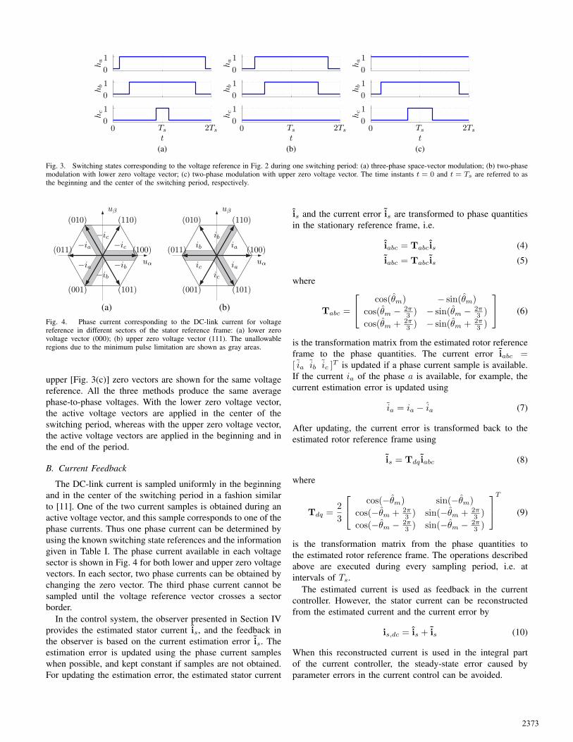
Fig. 3. Switching states corresponding to the voltage reference in Fig. 2 during one switching period: (a) three-phase space-vector modulation; (b) two-phasemodulation with lower zero voltage vector; (c) two-phase modulation with upper zero voltage vector. The time instants t = 0 and t = Ts are referred to asthe beginning and the center of the switching period, respectively.

uα

uβ

(100)

(110)(010)

(011)

(001) (101)

−ic−ic

−ia

−ia−ib

−ib uα

uβ

(100)

(110)(010)

(011)

(001) (101)

ia

ibib

icic

ia

(a) (b)

Fig. 4. Phase current corresponding to the DC-link current for voltagereference in different sectors of the stator reference frame: (a) lower zerovoltage vector (000); (b) upper zero voltage vector (111). The unallowableregions due to the minimum pulse limitation are shown as gray areas.

upper [Fig. 3(c)] zero vectors are shown for the same voltagereference. All the three methods produce the same averagephase-to-phase voltages. With the lower zero voltage vector,the active voltage vectors are applied in the center of theswitching period, whereas with the upper zero voltage vector,the active voltage vectors are applied in the beginning and inthe end of the period.

B. Current Feedback

The DC-link current is sampled uniformly in the beginningand in the center of the switching period in a fashion similarto [11]. One of the two current samples is obtained during anactive voltage vector, and this sample corresponds to one of thephase currents. Thus one phase current can be determined byusing the known switching state references and the informationgiven in Table I. The phase current available in each voltagesector is shown in Fig. 4 for both lower and upper zero voltagevectors. In each sector, two phase currents can be obtained bychanging the zero vector. The third phase current cannot besampled until the voltage reference vector crosses a sectorborder.

In the control system, the observer presented in Section IVprovides the estimated stator current is, and the feedback inthe observer is based on the current estimation error is. Theestimation error is updated using the phase current sampleswhen possible, and kept constant if samples are not obtained.For updating the estimation error, the estimated stator current

is and the current error is are transformed to phase quantitiesin the stationary reference frame, i.e.

iabc = Tabcis (4)

iabc = Tabcis (5)

where

Tabc =

cos(θm) − sin(θm)

cos(θm − 2π3 ) − sin(θm − 2π

3 )cos(θm + 2π

3 ) − sin(θm + 2π3 )

(6)

is the transformation matrix from the estimated rotor referenceframe to the phase quantities. The current error iabc =[ ia ib ic ]T is updated if a phase current sample is available.If the current ia of the phase a is available, for example, thecurrent estimation error is updated using

ia = ia − ia (7)

After updating, the current error is transformed back to theestimated rotor reference frame using

is = Tdq iabc (8)

where

Tdq =23

cos(−θm) sin(−θm)

cos(−θm + 2π3 ) sin(−θm + 2π

3 )cos(−θm − 2π

3 ) sin(−θm − 2π3 )

T

(9)

is the transformation matrix from the phase quantities tothe estimated rotor reference frame. The operations describedabove are executed during every sampling period, i.e. atintervals of Ts.

The estimated current is used as feedback in the currentcontroller. However, the stator current can be reconstructedfrom the estimated current and the current error by

is,dc = is + is (10)

When this reconstructed current is used in the integral partof the current controller, the steady-state error caused byparameter errors in the current control can be avoided.

2373

C. Minimum Pulse Limitation

The high rate of change of the inverter output voltage (i.e.high du/dt) during switching causes transients in the voltagesand currents of the inverter output phases. These transientsdisturb the current measurement during short inverter voltagepulses, and reliable current samples cannot be obtained shortlyafter switching. To improve the current measurement, theminimum duration of the voltage pulse, during which thecurrent is sampled, has to be lengthened. Consequently, shortactive voltage vectors cannot be used in the beginning and inthe center of the switching period. The effect of the minimumpulse limitation on the allowable stator voltage vector isdepicted in Fig. 4 for both lower and upper zero vectors.

The minimum pulse limitation distorts the stator voltage,especially at low stator voltage values (i.e. at low modulationindex values). The estimation errors of the stator current, rotorspeed, and rotor position caused by the voltage distortion arereduced by using the realizable (distorted) stator voltage in theadaptive observer described in Section IV.

IV. OBSERVER

A. Adaptive Observer

An adaptive observer [12] is used for the estimation of thestator current, rotor speed, and rotor position. The speed andposition estimation is based on the estimation error betweentwo different models; the actual motor can be considered as areference model and the observer—including the rotor speedestimate ωm—as an adjustable model. An error term used inan adaptation mechanism is based on the estimation error ofthe stator current. The estimated rotor speed, obtained by theadaptation mechanism, is fed back to the adjustable model.

The adaptive observer is formulated in the estimated rotorreference frame. The stator flux is selected as a state variablein the adjustable model,

˙ψs = us,ref − Rsis − ωmJψs + λis (11)

where estimated quantities are marked by ˆ and us,ref is thestator voltage reference. The estimate of the stator current is

is = L−1(ψs − ψpm) (12)

The current error is calculated based on available currentsamples as described in Section III-B. The feedback gainmatrix λ is varied as a function of the rotor speed [12].

The adaptation is based on an error term

Fε = [ 0 Lq ]is (13)

i.e. the current error in the estimated q direction is used foradaptation. The estimate of the electrical angular speed of therotor is obtained by a PI speed adaptation mechanism

ωm = −kpFε − ki

∫Fεdt (14)

where kp and ki are nonnegative gains. The estimate θm forthe rotor position is obtained by integrating ωm.

B. High-Frequency Signal Injection

Since the adaptive observer cannot perform well at lowspeeds due to inaccuracies in measurements and parameterestimates, an HF signal injection method is used to stabilizethe observer [13]. Originally, a carrier excitation signal alter-nating on the d axis at angular frequency ωc and having anamplitude uc, i.e.

uc1 = uc

[cos(ωct)

0

](15)

is superimposed on the voltage reference in the estimated rotorreference frame. An alternating current response is detected onthe q axis of the estimated rotor reference frame, amplitudemodulated by the rotor position estimation error θm = θm −θm. Demodulation and low-pass filtering results in an errorsignal ε that is approximately proportional to θm.

At low speeds and standstill, the stator voltage referencecan move between sectors too slowly for detecting all phasecurrents regularly. Although the HF excitation voltage in (15)results in varying voltage reference, different sectors may notbe covered equally enough. Consequently, one of the statorphase currents may be unavailable for a long period, and thesignal injection cannot detect the rotor position reliably. Forbetter sector coverage, a modified HF excitation voltage

uc2 = uc

[cos(ωct)sin(2ωct)

](16)

is proposed. Thus, the second harmonic of the excitationfrequency is injected to the q axis of the estimated rotorreference frame. The second harmonic appears in the statorcurrent, but it does not affect the error signal ε since thedemodulation is only sensitive to frequency ωc.

The error signal ε is used for correcting the estimatedposition by influencing the direction of the stator flux estimateof the adjustable model. The algorithm is given by

˙ψs,u = us,ref − Rsis − (ωm − ωε)Jψs,u + λis (17)

and

ωε = γpε+ γi

∫εdt (18)

where γp and γi are the nonnegative gains of the PI mechanismdriving the error signal ε to zero. At low speeds, both the signalinjection method and the adaptive observer contribute to therotor speed and position estimation. The influence of the HFsignal injection is decreased linearly with increasing speed,reaching zero at a certain speed [13]. At higher speeds, theestimation is based only on the adaptive observer.

It is important that the HF excitation voltage in (16) isincluded in the voltage reference fed to the adjustable modelin (17). The HF excitation voltage ensures reliable predictionof the HF current in the stator current estimate is, which isneeded for calculating the current error. It is to be noted thatthe reconstructed stator current is,dc (10) has to be used fordemodulation in the signal injection method instead of theestimated current is.

2374

TABLE IIMOTOR DATA

Nominal power 2.2 kWNominal voltage UN 370 VNominal current IN 4.3 ANominal frequency fN 75 HzNominal speed 1 500 r/minNominal torque TN 14.0 NmNumber of pole pairs p 3Stator resistance Rs 3.59 ΩDirect-axis inductance Ld 0.036 HQuadrature-axis inductance Lq 0.051 HPermanent magnet flux ψpm 0.545 VsTotal moment of inertia 0.015 kgm2

V. SIMULATION RESULTS

The proposed method was investigated by means of simu-lations and laboratory experiments. Fig. 1 shows the blockdiagram of the control system comprising cascaded speedand current control loops. PI-type speed control with activedamping is used. The current reference is,ref is calculatedaccording to maximum torque per current control. The currentcontrol is implemented as PI-type control in the estimated rotorreference frame.

The data of the six-pole interior-magnet PMSM (2.2 kW,1500 rpm) are given in Table II. The base values for voltage,current, and angular speed are defined as

√2/3UN ,

√2IN ,

and 2πfN , respectively. The electromagnetic torque is limitedto 22 Nm, which is 1.57 times the nominal torque TN . Thehigh-frequency carrier excitation signal has a frequency of 500Hz and an amplitude of 90 V. The HF signal injection is usedbelow the speed of 0.13 p.u. The speed control and currentcontrol bandwidths are 5 Hz and 200 Hz, respectively. Theobserver parameters were selected as in [12].

The MATLAB/Simulink environment was used for the simu-lations. The parameter values used in the controller were equalto those of the motor model. Fig. 5 shows results when theload torque was zero and the speed reference was changedstepwise from zero to 0.05 p.u. at t = 1 s., then reversed to−0.05 p.u. at t = 2 s., and finally set to zero at t = 3 s. Fig.5(a) shows results when the minimum duration of the invertervoltage pulses was not limited, and Fig. 5(b) shows resultswhen the duration was limited to 6 µs. Although the systemis stable in both cases, the effects of the distorted voltagecan be clearly seen in Fig. 5(b). Voltage reference samplescorresponding to the simulation in Fig. 5(b) are plotted inFig. 6 separately for the lower and the upper zero voltagevector. The areas that do not have voltage reference samplescorrespond to the unallowable regions illustrated in Fig. 4.The minimum pulse limitation is enabled in the followingsimulations and experiments.

The phase currents and the d- and q-axis current componentsare shown in Figs. 7 and 8, respectively, corresponding tothe simulation in Fig. 5(b). The HF current caused by theHF voltage signal is clearly visible in the figures. As can beseen in Fig. 7, the phase currents can be reliably estimatedalthough only few samples are obtained in each period of the

−0.08

0

0.08

−0.8

0

0.8

0 1 2 3 4−20

0

20

ωm

(p.u.)

T/T

Nθ m

()

t (s)

(a)

−0.08

0

0.08

−0.8

0

0.8

0 1 2 3 4−20

0

20ω

m(p.u.)

T/T

Nθ m

()

t (s)

(b)

Fig. 5. Simulation results showing speed reference steps at no load: (a) min-imum duration of voltage pulse not limited; (b) minimum duration of voltagepulse limited to 6 µs. First subplot shows electrical angular speed (solid),its estimate (dashed), and its reference (dash-dotted). Second subplot showsestimated electromagnetic torque (solid) and load torque reference (dash-dotted). Last subplot shows estimation error of rotor position in electricaldegrees.

−0.4 0 0.4−0.4

0

0.4

−0.4 0 0.4−0.4

0

0.4

uβ

,ref

(p.u.)

uα,ref (p.u.)

(a)

uβ

,ref

(p.u.)

uα,ref (p.u.)

(b)

Fig. 6. Voltage references in the stator reference frame from the simulationin Fig. 5(b): (a) lower zero voltage vector; (b) upper zero voltage vector.

HF signal. Fig. 8 shows that the estimated and reconstructedcurrents follow the actual values well even during a transientstate (speed reversal). The difference between the estimatedand reconstructed d-axis current components is due to thecurrent estimation error, which is commonly present duringa transient. However, it is to be noted that the reconstructedcurrents follow the actual currents with good accuracy.

2375

−0.12

0

0.12

−0.12

0

0.12

1.5 1.502 1.504 1.506 1.508 1.51−0.12

0

0.12

i a(p.u.)

i b(p.u.)

i c(p.u.)

t (s)

Fig. 7. Phase currents from the simulation in Fig. 5(b). First subplot showsphase a current, second subplot shows phase b current, and third subplot showsphase c current. Actual phase current is shown as solid line and reconstructedcurrent as dashed line. The circles indicate samples obtained from the phasecurrent.

−0.2

0

0.2

1.995 2 2.005 2.01 2.015−0.8

00.2

i d(p.u.)

i q(p.u.)

t (s)

Fig. 8. Currents id and iq from the simulation in Fig. 5(b). First subplotshows d-axis current, second subplot shows q-axis current. Phase currentsconverted to the estimated rotor reference frame are shown as solid line,estimated currents id and iq as dashed line, and reconstructed currents id,dc

and iq,dc as dash-dotted line, which mostly overlaps the solid line.

Simulation results at zero speed reference are shown inFig. 9. The load torque was changed stepwise from zero tothe positive nominal value at t = 1 s, then reversed to thenegative nominal value at t = 2 s, and finally set to zero att = 3 s. The drive is stable, and the rotor position estimationerror remains small, indicating good dynamic performance.Sustained operation at zero speed under load is also possible.Fig. 10 depicts simulation results during a slow speed reversalfrom ωm,ref = 0.2 p.u. to ωm,ref = −0.2 p.u. between t = 1 sand t = 9 s. The ripple visible in the curves is due to the statorvoltage distortion caused by the minimum pulse limitation. Inspite of the ripple, the system is stable in the speed reversal.

VI. EXPERIMENTAL RESULTS

The experimental setup is illustrated in Fig. 11. In thelaboratory tests, the 2.2-kW PMSM described in Section Vwas fed by a commercial frequency converter with modifiedcontrol software. Mechanical load is provided by a PMSMservo drive, and the actual rotor speed and position aremonitored by an incremental encoder. The DC-link currentis measured by a shunt resistor, and the control algorithms

−0.2

0

0.2

−1.8

0

1.8

0 1 2 3 4−20

0

20

ωm

(p.u.)

T/T

Nθ m

()

t (s)

Fig. 9. Simulation results showing load torque steps at zero speed reference.Explanations of the curves are as in Fig. 5.

−0.25

0

0.25

−1.6

0

1.6

0 2 4 6 8 10−20

0

20

ωm

(p.u.)

T/T

Nθ m

()

t (s)

Fig. 10. Simulation results showing slow speed reversal at nominal loadtorque. Explanations of the curves are as in Fig. 5.

are implemented in a Texas Instruments TMS320F2811 DSP.The two-phase modulation scheme with synchronized currentsampling is used. The commutation delays in the inverterbridge and the control delays of the IGBTs are compensatedin a feedforward manner when calculating the switch turnreferences of the IGBTs. The minimum length of the voltagepulse in the beginning and in the middle of the switchingperiod is limited to 6 µs in the modulator.

The nominal DC-link voltage is 540 V, the switchingfrequency 4 kHz, and the sampling frequency 8 kHz. In theexperiments, the q-axis current reference was used to controlthe torque, and the d-axis current reference was set to zero.Due to practical restrictions, data could be captured from thecontrol software to the computer only at an approximate rateof 15 samples in a second for each variable. An anti-aliasingfilter having a bandwidth of 10 Hz was applied to the recordedvariables. The actual rotor speed and position were monitored,and a faster transfer rate was used for these variables.

Fig. 12 shows experimental results under nominal load. Thespeed reference is changed stepwise from zero to 0.5 p.u. insteps of 0.125 p.u. Each step has a duration of 2 seconds.Finally, the speed reference is set to zero at t = 10 s. Thesystem can cope with stepwise changes in the speed reference,

2376

PMSM Servo

Computer

Freq.conv.

Freq.conv.

Speed formonitoring

Fig. 11. Experimental setup. Mechanical load is provided by a servo drive.

0

0.25

0.5

0

0.8

1.6

0 2 4 6 8 10 12−200

0

200

ωm

(p.u.)

T/T

Nθ m

()

t (s)

Fig. 12. Experimental results showing speed reference steps under nominalload torque. First subplot shows electrical angular speed (solid), its estimate(dashed), and its reference (dash-dotted). Second subplot shows estimatedelectromagnetic torque (solid) and load torque reference (dash-dotted). Lastsubplot shows true rotor position in electrical degrees.

and the operation is stable from zero speed to high speeds.Experimental results showing nominal load torque steps at

zero speed reference are depicted in Fig. 13. A positive loadtorque is applied between t = 2 s and t = 4 s, and a negativeload torque is applied between t = 6 s and t = 8 s. Theproposed method allows sustained operation at zero speedunder nominal load, and is robust to fast load torque changes.

VII. CONCLUSIONS

The proposed method is suitable for vector control ofPMSM drives when only the DC-link current is measuredinstead of the motor phase currents. A two-phase PWMmethod is used, allowing the phase currents to be sampledat uniform intervals. An adaptive observer is used for theestimation, and the current error used for feedback is up-dated using available phase current samples. The low-speedoperation is stabilized by an HF signal injection method witha modified excitation voltage, and the adaptive observer isused for estimating the HF current response. The proposedmethod enables reliable estimation of the stator current, rotorspeed, and rotor position, and is also insusceptible to the statorvoltage distortion caused by the minimum pulse limitation.The simulation and experimental results presented in the papershow that the proposed method can operate in a wide speedrange and can cope with transients in the speed reference andin the load torque.

−0.1

0

0.1

−1.5

0

1.5

0 2 4 6 8 10−200

0

200

ωm

(p.u.)

T/T

Nθ m

()

t (s)

Fig. 13. Experimental results showing load torque steps at zero speedreference. Explanations of the curves are as in Fig. 12.

ACKNOWLEDGEMENT

The authors gratefully acknowledge the financial supportgiven by ABB Oy, Walter Ahlstrom Foundation, and KAUTEFoundation.

REFERENCES

[1] T. C. Green and B. W. Williams, “Derivation of motor line-currentwaveforms from the DC-link current of an inverter,” Proc. Inst. Elect.Eng. B, vol. 136, no. 4, pp. 196–204, July 1989.

[2] T. Habetler and D. M. Divan, “Control strategies for direct torque controlusing discrete pulse modulation,” IEEE Trans. Ind. Applicat., vol. 27,no. 5, pp. 893–901, Sept./Oct. 1991.

[3] J. F. Moynihan, S. Bolognani, R. C. Kavanagh, M. G. Egan, and J. M. D.Murphy, “Single sensor current control of ac servodrives using digitalsignal processors,” in Proc. EPE’93, vol. 4, Brighton, UK, Sept. 1993,pp. 415–421.

[4] F. Blaabjerg, J. K. Pedersen, U. Jaeger, and P. Thoegersen, “Singlecurrent sensor technique in the DC link of three-phase PWM-VSinverters: a review and a novel solution,” IEEE Trans. Ind. Applicat.,vol. 33, no. 5, pp. 1241–1253, Sept./Oct. 1997.

[5] S. N. Vukosavic and A. M. Stankovic, “Sensorless induction motordrive with a single DC-link current sensor and instantaneous active andreactive power feedback,” IEEE Trans. Ind. Electron., vol. 48, no. 1, pp.195–204, Feb. 2001.

[6] U.-H. Rieder, M. Schroedl, and A. Ebner, “Sensorless control of anexternal rotor PMSM in the whole speed range including standstill usingDC-link measurements only,” in Proc. IEEE PESC’04, vol. 2, Aachen,Germany, June 2004, pp. 1280– 1285.

[7] H. Kim and T. M. Jahns, “Phase current reconstruction for AC motordrives using a DC link single current sensor and measurement voltagevectors,” IEEE Trans. Pow. Electron., vol. 21, no. 5, pp. 1413–1419,Sept. 2006.

[8] M. Depenbrock, “Pulse width control of a 3-phase inverter with nonsi-nusoidal phase voltages,” in Proc. IEEE ISPC’77, 1977, pp. 399–403.

[9] S. Ogasawara, H. Akagi, and A. Nabae, “A novel PWM scheme ofvoltage source inverters based on space vector theory,” in Proc. EPE’89,vol. 1, Aachen, Germany, Oct. 1989, pp. 1197–1202.

[10] J. W. Kolar, H. Ertl, and F. C. Zach, “Influence of the modulation methodon the conduction and switching losses of a PWM converter system,”IEEE Trans. Ind. Applicat., vol. 27, no. 6, pp. 1063–1075, Nov./Dec.1991.

[11] P. Virolainen, S. Heikkila, and M. Hinkkanen, “Method for determiningoutput currents of frequency converter,” Finnish Patent FI 116 337 B,Oct. 31, 2005.

[12] A. Piippo, M. Hinkkanen, and J. Luomi, “Analysis of an adaptive ob-server for sensorless control of PMSM drives,” in Proc. IEEE IECON’05,Raleigh, NC, Nov. 2005, pp. 1474–1479.

[13] A. Piippo and J. Luomi, “Adaptive observer combined with HF sig-nal injection for sensorless control of PMSM drives,” in Proc. IEEEIEMDC’05, San Antonio, TX, May 2005, pp. 674–681.

2377