Design of a fault-tolerant controller based on observers for a PMSM drive

1416 IEEE TRANSACTIONS ON INDUSTRIAL ELECTRONICS, VOL. 58, NO. 4, APRIL 2011

Design of a Fault-Tolerant Controller Based onObservers for a PMSM Drive

Ahmad Akrad, Mickaël Hilairet, Member, IEEE, and Demba Diallo, Senior Member, IEEE

Abstract—This paper presents a specific controller architec-ture devoted to obtain a permanent-magnet synchronous motor(PMSM) drive that is robust to mechanical sensor failure. In orderto increase the reliability which is a key issue in industrial andtransportation applications (electric or hybrid ground vehicle oraerospace actuators), two virtual sensors (a two-stage extendedKalman filter and a back-electromotive-force adaptive observer)and a maximum-likelihood voting algorithm are combined withthe actual sensor to build a fault-tolerant controller (FTC). Theobservers are evaluated through simulation and experimentalresults. The FTC feasibility is proved through simulations andexperiments on a 1.1-kW PMSM drive.

Index Terms—Adaptive observer (AO), fault-tolerant controller(FTC), Kalman filter, mechanical sensor failure, permanent-magnet synchronous motors (PMSMs), sensorless control.

I. INTRODUCTION

S EVERAL failures afflict electrical motor drives, and sofar, redundant or conservative design has been used in

every application where continuity of operations is a key fea-ture. This is the case of home and civil appliances, such asair conditioning/heat pumps, engine cooling fans, and electricvehicles (EVs), where reliability is a key issue. Fault tolerancehas become an increasingly interesting topic in the last decadewhere the automation has become more complex. The objectiveis to give solutions that provide fault accommodation to themost frequent faults and thereby reduce the costs of handlingthe faults. In submerged pumps or hostile environments whereaccessibility to the drive and to the sensors is tedious and,nevertheless, continuity of operation is mandatory even incase of fault occurrence, a sensorless algorithm is indispens-able to maintain the availability and therefore increase thereliability.

Due to its capability of field-weakening control, high effi-ciency, and high power density, permanent-magnet synchro-nous motors (PMSMs) are becoming competitive in manyapplications such as railway electric propulsion power trains,EVs, or hybrid EVs [1], [2].

Manuscript received October 2, 2009; revised February 12, 2010; acceptedApril 9, 2010. Date of current version March 11, 2011.

The authors are with the Laboratoire de Génie Electrique de Paris/SPEE-Labs, CNRS UMR 8507–École Supérieure d’Électricité (SUPELEC)–Université Pierre et Marie Curie P6–Université Paris-Sud 11, 91192 Gif-sur-Yvette, France (e-mail: [email protected]; [email protected]; [email protected]).

Color versions of one or more of the figures in this paper are available onlineat http://ieeexplore.ieee.org.

Digital Object Identifier 10.1109/TIE.2010.2050756

There are numerous study results about fault detection andfault-tolerant control [3]–[10], but most of them focused on thefaults of power semiconductors of an inverter [3] and statorwindings [4] of the motor. In [8], a fault-tolerant controller(FTC) for automotive applications with an induction machinehas been presented. The proposed system adaptively changesthe control technique in the event of sensor failure or recovery.In [9], a method to detect sensor faults and an algorithm toreconfigure the control system for interior permanent-magnetmotor drives have been described. The study focused on thedetection of current sensor faults, the analysis of a currentobserver, and the resilient control of the drive system whileretaining the same basic control strategy.

In this paper, an active position-sensor FTC is presented. It isbased on the combination of the actual sensor and two virtualones [a two-stage extended Kalman filter (EKF) and a back-electromotive-force (EMF) adaptive observer (AO)]. A votingalgorithm (maximum likelihood) parameterized with reliabilitycoefficients dedicated to each sensor on the whole speed rangeselects the appropriate input (speed and position) for the controlloops [11].

This paper is composed of three sections. The second sectionis dedicated to the description of the sensorless algorithms andtheir experimental validation. The sensitivity analysis againstparameter variation of the position and speed estimators isstudied through intensive simulations. In the third section,the FTC architecture is introduced; the sensor and its faultsare presented. The proposed FTC performance is detailed inthe fourth section, where simulations and experiments arepresented.

II. POSITION AND SPEED OBSERVERS

PMSM drive research has been concentrated on the elimi-nation of the mechanical sensors at the motor shaft withoutdeteriorating the dynamic performance of the drive-controlsystem [12]–[15]. The advantages of sensorless ac drives arethe lower cost, reduced size of the motor set, cable elimination,and increased reliability [16].

The position and speed estimations are computed by anoptimal two-stage EKF (OTSEKF) and a back-EMF AO. Thefirst observer is designed in the (dq) rotating frame, whilethe second one is based on a model in the (αβ) referenceframe. The two observers use the same information, i.e., thecurrent measurements (isα, isβ) and the controller-output volt-ages (vsα, vsβ) in order to give an estimate of the mechanicalposition and speed.

0278-0046/$26.00 © 2011 IEEE

AKRAD et al.: DESIGN OF A FAULT-TOLERANT CONTROLLER BASED ON OBSERVERS FOR A PMSM DRIVE 1417

A. Two-Stage EKF

1) Continuous Motor Model: The salient PMSM is modeledin the standard (dq) reference frame as follows:

d

dtX(t) = Ac(Θ)X(t) + Bu

c (Θ)U(t) + BΘc (Θ)Θ(t)

Y (t) = C(Θ)X(t) (1)

with

X = [ isd isq ]t Θ = [ω θ ]t

U = [ vsα vsβ ]t Y = [ isα isβ ]t

Ac(Θ) =

[−Rs

Ld

ωLq

Ld

−ωLd

Lq−Rs

Lq

]Bu

c (Θ) =

[cos(θ)

Ld

sin(θ)Ld

− sin(θ)Lq

cos(θ)Lq

]

BΘc (Θ) =

[0 0

− ψLq

0

]C(Θ) =

[cos(θ) − sin(θ)sin(θ) cos(θ)

].

In these equations, vsα, vsβ , isα, and isβ are the voltages andcurrents in the (αβ) reference frame, isd and isq are currentsin the (dq) frame, Ld and Lq are the stator inductances, Rs

is the stator winding resistance, and ψ is the flux produced bythe magnets. The angular velocity ω is measured in electricalradians per second (the connection between electrical and me-chanical variables is ω = PΩ, where P is the number of polepairs), and θ is the electrical position.

2) Discretization of the Motor Model: For the digital imple-mentation of an estimator, a discrete-time state-space model isrequired. Provided that the input vector U is nearly constantduring a sampling period Ts (Ts = 50 μs) and a small dis-cretization error is tolerated, a first-order series expansion ofthe matrix exponential is used

eAc Ts ≈A = I + Ac Ts

A−1c (eAc Ts − I)Bc ≈B = Ts Bc.

The previous continuous model (1) leads to the followingdiscrete-time state-space model

X[k + 1] = A(Θ)X[k] + Bu(Θ)U [k] + BΘ(Θ)Θ[k]

Y [k] = C(Θ)X[k]

with

A(Θ) =

[1 − Rs

LdTs

ωLq

LdTs

−ωLd

LqTs 1 − Rs

LqTs

]

Bu(Θ) =

[cos(θ)

LdTs

sin(θ)Ld

Ts

− sin(θ)Lq

Tscos(θ)

LqTs

]

BΘ(Θ) =[

0 0− ψ

LqTs 0

].

This discretized model will be used in the prediction step ofthe EKF which is designed to estimate the unknown vector Θpreviously defined.

3) OTSEKF Algorithm: The main objective of the estimatoris to determine the position and speed of the PMSM. Therefore,

those two variables must be concatenated with the previousstate vector X. This leads to an augmented observer with astate-space vector composed of the currents, the speed, and theposition. Treating X[k] as the full-order state and Θ[k] as theunknown states, the state-space model is described by

Xa[k + 1] =A (Θ[k]) Xa[k] + B (Θ[k]) U [k] + w[k]

Y [k] =C (Θ[k]) Xa[k] + By (Θ[k]) U [k] + η[k] (2)

with

Xa[k] =[

X[k]Θ[k]

]

A (Θ[k]) =[

A (Θ[k]) BΘ(Θ[k])0 G(Θ[k])

]

B (Θ[k]) =[

Bu (Θ[k])0

]By =

[0 00 0

]

C (Θ[k]) = [C (Θ[k]) D (Θ[k]) ]

W [k] =[

W x[k]WΘ[k]

]

where G(Θ[k]) describes the evolution of the unknown statevariable Θ between two time samples.

The application of the EKF [18] to the nonlinear state-spacemodel (2) is described as follows:

Xa[k|k − 1] = A[k − 1]Xa[k − 1|k − 1] + B[k − 1]U [k − 1]

P [k|k − 1] = F [k − 1]P [k − 1|k − 1]Ft[k − 1] + Q[k − 1]

K[k] = P [k|k − 1]Ht[k]

+(H[k]P [k|k − 1]H

t[k] + R[k]

)−1

Xa[k|k] = Xa[k|k − 1] + K[k]

×(Y [k] − H[k]Xa[k|k − 1] − By[k]U [k]

)P [k|k] = P [k|k − 1] − K[k]H[k]P [k|k − 1]

with

F [k] =[

F (Θ[k]) E (Θ[k])0 G (Θ[k])

]

H[k] = [H1 (Θ[k]) H2 (Θ[k]) ]

F (Θ[k]) =∂

∂X

(A (Θ[k]) X[k] + BΘ (Θ[k]) Θ[k]

+ Bu (Θ[k]) U [k])

= A (Θ[k])

E (Θ[k]) =∂

∂Θ(A (Θ[k]) X[k] + BΘ (Θ[k]) Θ[k]

+ Bu (Θ[k]) U [k])

E (Θ[k]) =

[isqLq

LdTs

vsq

LdTs

− ψLq

Ts − isdLd

LqTs − vsd

LqTs

]

G (Θ[k]) =[

1 0Ts 1

]D (Θ[k]) =

[0 00 0

]


H1 (Θ[k]) =∂

∂X

(C (Θ[k]) X[k] + D (Θ[k]) Θ[k]

+ By (Θ[k]) U [k])

= C (Θ[k])

H2 (Θ[k]) =∂

∂Θ(C (Θ[k]) X[k] + D (Θ[k]) Θ[k]

+ By (Θ[k]) U [k])

H2 (Θ[k]) =[

0 − sin(θ)isd − cos(θ)isq

0 cos(θ)isd − sin(θ)isq

]

K[k] =[

Kx[k]KΘ[k]

]

P [·] =[

P x[·] P xΘ[·](P xΘ[·]

)tPΘ[·]

]

Q[k] =[

Qx[k] QxΘ[k](QxΘ[k]

)tQΘ[k]

]

where vsd = cos(θ)vsα + sin(θ)vsβ and vsq = − sin(θ)vsα +cos(θ)vsβ are voltages in the (dq) frame.

The covariance matrices Q and R characterize the noisesw and η, which take into account the model approximationsand the measurement errors. Some authors use a physicalapproach to obtain a more realistic tuning that allows one toroughly evaluate the state and parameter uncertainties [17].However, a fine evaluation of the matrices is very difficult,and generally, a simplified analysis is used. Without additionalinformation, the noises are considered as uncorrelated, timeindependent, and free-tuning parameters, yielding a block-diagonal matrix Q[k] = diag(Qx[k], QΘ[k]). Since the Kalmangain is not modified when both Q and R are multiplied bya scalar and the components on the α and β axes can beconsidered as statistically orthogonal and there is no reasonto consider differently the elements of the pair (isα, isβ), werestrict ourselves to only 3 DOF

R =[

1 00 1

]Q =

⎡⎢⎣

α1 0 0 00 α1 0 00 0 α2 00 0 0 α3

⎤⎥⎦ .

The EKF has a heavier computational cost with a roughimplementation. Therefore, an alternative solution is used inorder to reduce the computation time [20], [21]: two-stage EFK(OTSEKF).

The nonlinear OTSEKF is obtained by using a transfor-mation T [·] and two matrices M [k] and N [k], so that thevariance–covariance matrices P [·] are now diagonal [19]–[21](overlined expressions correspond to vectors and matrices in thenew base)

T (J) =[

I J0 I

]P [·] =

[P

x[·] 0

0 PΘ[·]

]

Xa[k|k − 1] =T (M [k]) Xa[k|k − 1]

P [k|k − 1] =T (M [k]) P [k|k − 1]T (M [k])t

Xa[k|k] =T (N [k]) Xa[k|k]

K[k] =T (N [k]) K[k]

P [k|k] =T (N [k]) P [k|k]T (N [k])t .

Fig. 1. Back-EMF AO diagram.

Finally, the nonlinear OTSEKF equations are as follows.

1) State and parameter prediction

X[k|k − 1] =A[k − 1]X[k − 1|k − 1]

+ Bu[k − 1]U [k − 1] + u[k − 1]

u[k − 1] =(A[k − 1]N [k − 1] + BΘ[k − 1]

− M [k]G[k − 1])Θ[k − 1|k − 1]

Θ[k|k − 1] =G[k − 1]Θ[k − 1|k − 1]

Px[k|k − 1] =F [k − 1]P

x[k − 1|k − 1]F [k − 1]t + Q

x[k]

Qx[k] =Qx[k] − QxΘ[k]M [k + 1]t

− M [k + 1](QxΘ[k] − M [k + 1]QΘ[k]

)t

M [k] =M [k] +(QxΘ − M [k]QΘ

)P

Θ[k|k − 1]−1

M [k] =(F [k − 1]N [k − 1] + E[k − 1]Θ[k−1|k−1]

)× G[k − 1]−1

E[k] =∂

∂Θ(A[k]

(X[k] + N [k]Θ[k]

)+ BΘ[k] Θ[k] + Bu[k]U [k]

)Θ[k|k]

PΘ[k|k − 1] =G[k − 1]P

Θ[k − 1|k − 1]G[k − 1]t + QΘ[k].

2) State and parameter correction

X[k|k] =X[k|k − 1] + Kx[k]

×(Y [k] − C[k]X[k|k − 1]

− (S − S)Θ[k|k − 1] − By[k]U [k])

Kx[k] =P

x[k|k − 1]H1[k]t

×(H1[k]P

x[k|k − 1]H1[k]t + R

)−1

Px[k|k] =P

x[k|k − 1] − K

x[k]H1[k]P

x[k|k − 1]

Θ[k|k] =Θ[k|k − 1] + KΘ

[k]

×(Y [k] − C[k]X[k|k − 1]

− S[k]Θ[k|k − 1] − By[k]U [k])

KΘ[k] =P

Θ[k|k − 1]S[k]t

×(H1[k]P

x[k|k − 1]H1[k]t

+ R[k] + S[k]PΘ[k|k − 1]S[k]t

)−1

PΘ[k|k] =P

Θ[k|k − 1] − K

Θ[k]S[k]P

Θ[k|k − 1]

S[k] =H1[k]M [k] + H2[k]

S[k] =C[k]M [k] + D[k].


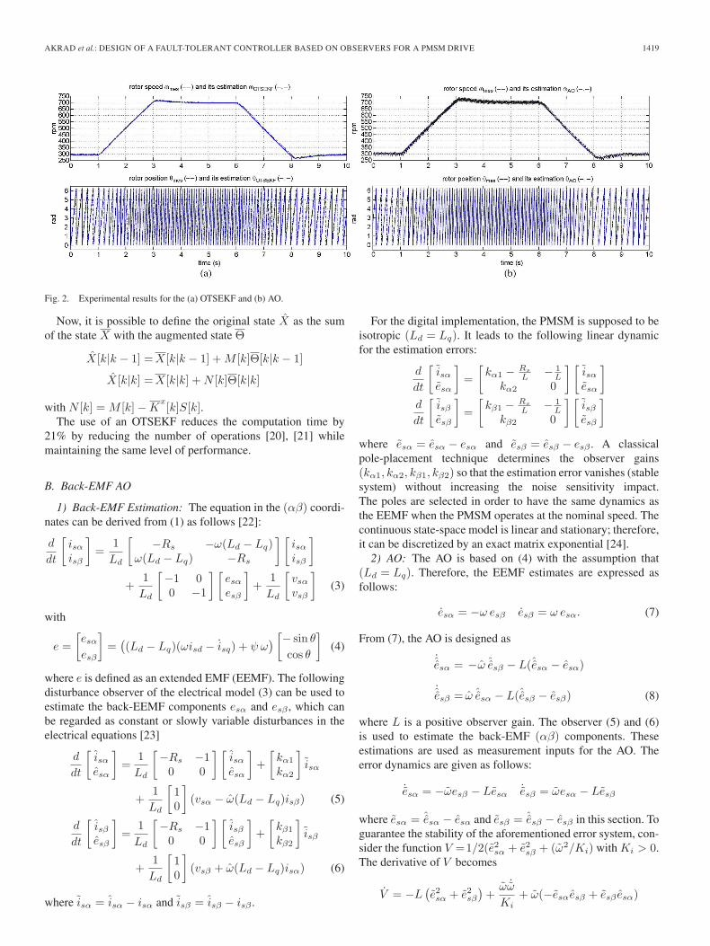
Fig. 2. Experimental results for the (a) OTSEKF and (b) AO.

Now, it is possible to define the original state X as the sumof the state X with the augmented state Θ

X[k|k − 1] =X[k|k − 1] + M [k]Θ[k|k − 1]

X[k|k] =X[k|k] + N [k]Θ[k|k]

with N [k] = M [k] − Kx[k]S[k].

The use of an OTSEKF reduces the computation time by21% by reducing the number of operations [20], [21] whilemaintaining the same level of performance.

B. Back-EMF AO

1) Back-EMF Estimation: The equation in the (αβ) coordi-nates can be derived from (1) as follows [22]:

d

dt

[isα

isβ

]=

1Ld

[−Rs −ω(Ld − Lq)

ω(Ld − Lq) −Rs

] [isα

isβ

]

+1Ld

[−1 00 −1

] [esα

esβ

]+

1Ld

[vsα

vsβ

](3)

with

e =[esα

esβ

]=

((Ld − Lq)(ωisd − isq) + ψ ω

) [− sin θ

cos θ

](4)

where e is defined as an extended EMF (EEMF). The followingdisturbance observer of the electrical model (3) can be used toestimate the back-EEMF components esα and esβ , which canbe regarded as constant or slowly variable disturbances in theelectrical equations [23]

d

dt

[isα

esα

]=

1Ld

[−Rs −1

0 0

] [isα

esα

]+

[kα1

kα2

]isα

+1Ld

[10

](vsα − ω(Ld − Lq)isβ) (5)

d

dt

[isβ

esβ

]=

1Ld

[−Rs −1

0 0

] [isβ

esβ

]+

[kβ1

kβ2

]isβ

+1Ld

[10

](vsβ + ω(Ld − Lq)isα) (6)

where isα = isα − isα and isβ = isβ − isβ .

For the digital implementation, the PMSM is supposed to beisotropic (Ld = Lq). It leads to the following linear dynamicfor the estimation errors:

d

dt

[isα

esα

]=

[kα1 − Rs

L − 1L

kα2 0

] [isα

esα

]d

dt

[isβ

esβ

]=

[kβ1 − Rs

L − 1L

kβ2 0

] [isβ

esβ

]

where esα = esα − esα and esβ = esβ − esβ . A classicalpole-placement technique determines the observer gains(kα1, kα2, kβ1, kβ2) so that the estimation error vanishes (stablesystem) without increasing the noise sensitivity impact.The poles are selected in order to have the same dynamics asthe EEMF when the PMSM operates at the nominal speed. Thecontinuous state-space model is linear and stationary; therefore,it can be discretized by an exact matrix exponential [24].

2) AO: The AO is based on (4) with the assumption that(Ld = Lq). Therefore, the EEMF estimates are expressed asfollows:

esα = −ω esβ esβ = ω esα. (7)

From (7), the AO is designed as

˙esα = −ω êsβ − L(êsα − esα)

˙esβ = ω êsα − L(êsβ − esβ) (8)

where L is a positive observer gain. The observer (5) and (6)is used to estimate the back-EMF (αβ) components. Theseestimations are used as measurement inputs for the AO. Theerror dynamics are given as follows:

˙esα = −ωesβ − Lesα˙esβ = ωesα − Lesβ

where esα = êsα − esα and esβ = êsβ − esβ in this section. Toguarantee the stability of the aforementioned error system, con-sider the function V =1/2(e2

sα + e2sβ + (ω2/Ki) with Ki > 0.

The derivative of V becomes

V = −L(e2sα + e2

sβ

)+

ω ˙ωKi

+ ω(−esαesβ + esβ esα)


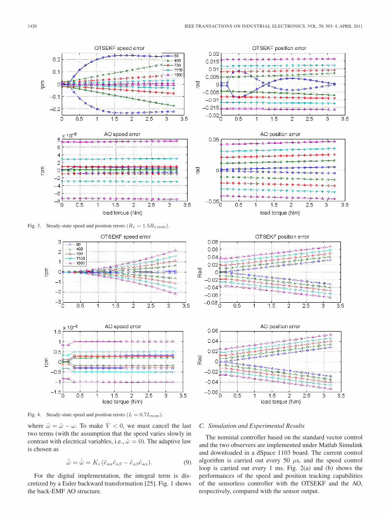
Fig. 3. Steady-state speed and position errors (Rs = 1.5Rs nom).

Fig. 4. Steady-state speed and position errors (L = 0.7Lnom).

where ω = ω − ω. To make V < 0, we must cancel the lasttwo terms (with the assumption that the speed varies slowly incontrast with electrical variables, i.e., ω = 0). The adaptive lawis chosen as

˙ω = ˙ω = Ki (esαesβ − esβ esα). (9)

For the digital implementation, the integral term is dis-cretized by a Euler backward transformation [25]. Fig. 1 showsthe back-EMF AO structure.

C. Simulation and Experimental Results

The nominal controller based on the standard vector controland the two observers are implemented under Matlab Simulinkand downloaded in a dSpace 1103 board. The current controlalgorithm is carried out every 50 μs, and the speed controlloop is carried out every 1 ms. Fig. 2(a) and (b) shows theperformances of the speed and position tracking capabilitiesof the sensorless controller with the OTSEKF and the AO,respectively, compared with the sensor output.


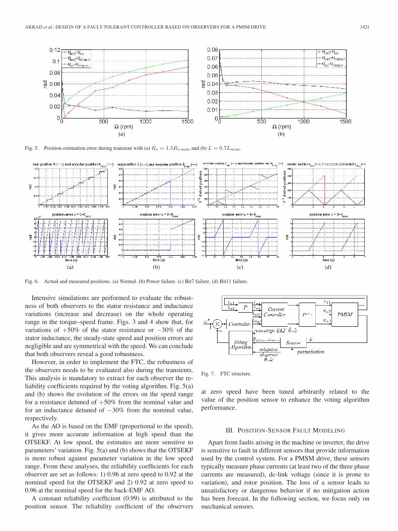
Fig. 5. Position estimation error during transient with (a) Rs = 1.5Rs nom and (b) L = 0.7Lnom.

Fig. 6. Actual and measured positions. (a) Normal. (b) Power failure. (c) Bit7 failure. (d) Bit11 failure.

Intensive simulations are performed to evaluate the robust-ness of both observers to the stator resistance and inductancevariations (increase and decrease) on the whole operatingrange in the torque–speed frame. Figs. 3 and 4 show that, forvariations of +50% of the stator resistance or −30% of thestator inductance, the steady-state speed and position errors arenegligible and are symmetrical with the speed. We can concludethat both observers reveal a good robustness.

However, in order to implement the FTC, the robustness ofthe observers needs to be evaluated also during the transients.This analysis is mandatory to extract for each observer the re-liability coefficients required by the voting algorithm. Fig. 5(a)and (b) shows the evolution of the errors on the speed rangefor a resistance detuned of +50% from the nominal value andfor an inductance detuned of −30% from the nominal value,respectively.

As the AO is based on the EMF (proportional to the speed),it gives more accurate information at high speed than theOTSEKF. At low speed, the estimates are more sensitive toparameters’ variation. Fig. 5(a) and (b) shows that the OTSEKFis more robust against parameter variation in the low speedrange. From these analyses, the reliability coefficients for eachobserver are set as follows: 1) 0.96 at zero speed to 0.92 at thenominal speed for the OTSEKF and 2) 0.92 at zero speed to0.96 at the nominal speed for the back-EMF AO.

A constant reliability coefficient (0.99) is attributed to theposition sensor. The reliability coefficient of the observers

Fig. 7. FTC structure.

at zero speed have been tuned arbitrarily related to thevalue of the position sensor to enhance the voting algorithmperformance.

III. POSITION-SENSOR FAULT MODELING

Apart from faults arising in the machine or inverter, the driveis sensitive to fault in different sensors that provide informationused by the control system. For a PMSM drive, these sensorstypically measure phase currents (at least two of the three phasecurrents are measured), dc-link voltage (since it is prone tovariation), and rotor position. The loss of a sensor leads tounsatisfactory or dangerous behavior if no mitigation actionhas been forecast. In the following section, we focus only onmechanical sensors.


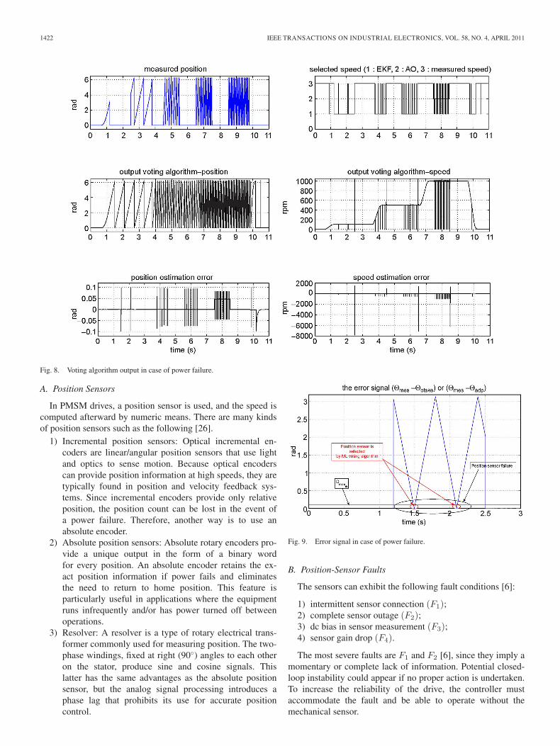
Fig. 8. Voting algorithm output in case of power failure.

A. Position Sensors

In PMSM drives, a position sensor is used, and the speed iscomputed afterward by numeric means. There are many kindsof position sensors such as the following [26].

1) Incremental position sensors: Optical incremental en-coders are linear/angular position sensors that use lightand optics to sense motion. Because optical encoderscan provide position information at high speeds, they aretypically found in position and velocity feedback sys-tems. Since incremental encoders provide only relativeposition, the position count can be lost in the event ofa power failure. Therefore, another way is to use anabsolute encoder.

2) Absolute position sensors: Absolute rotary encoders pro-vide a unique output in the form of a binary wordfor every position. An absolute encoder retains the ex-act position information if power fails and eliminatesthe need to return to home position. This feature isparticularly useful in applications where the equipmentruns infrequently and/or has power turned off betweenoperations.

3) Resolver: A resolver is a type of rotary electrical trans-former commonly used for measuring position. The two-phase windings, fixed at right (90◦) angles to each otheron the stator, produce sine and cosine signals. Thislatter has the same advantages as the absolute positionsensor, but the analog signal processing introduces aphase lag that prohibits its use for accurate positioncontrol.

Fig. 9. Error signal in case of power failure.

B. Position-Sensor Faults

The sensors can exhibit the following fault conditions [6]:

1) intermittent sensor connection (F1);2) complete sensor outage (F2);3) dc bias in sensor measurement (F3);4) sensor gain drop (F4).

The most severe faults are F1 and F2 [6], since they imply amomentary or complete lack of information. Potential closed-loop instability could appear if no proper action is undertaken.To increase the reliability of the drive, the controller mustaccommodate the fault and be able to operate without themechanical sensor.


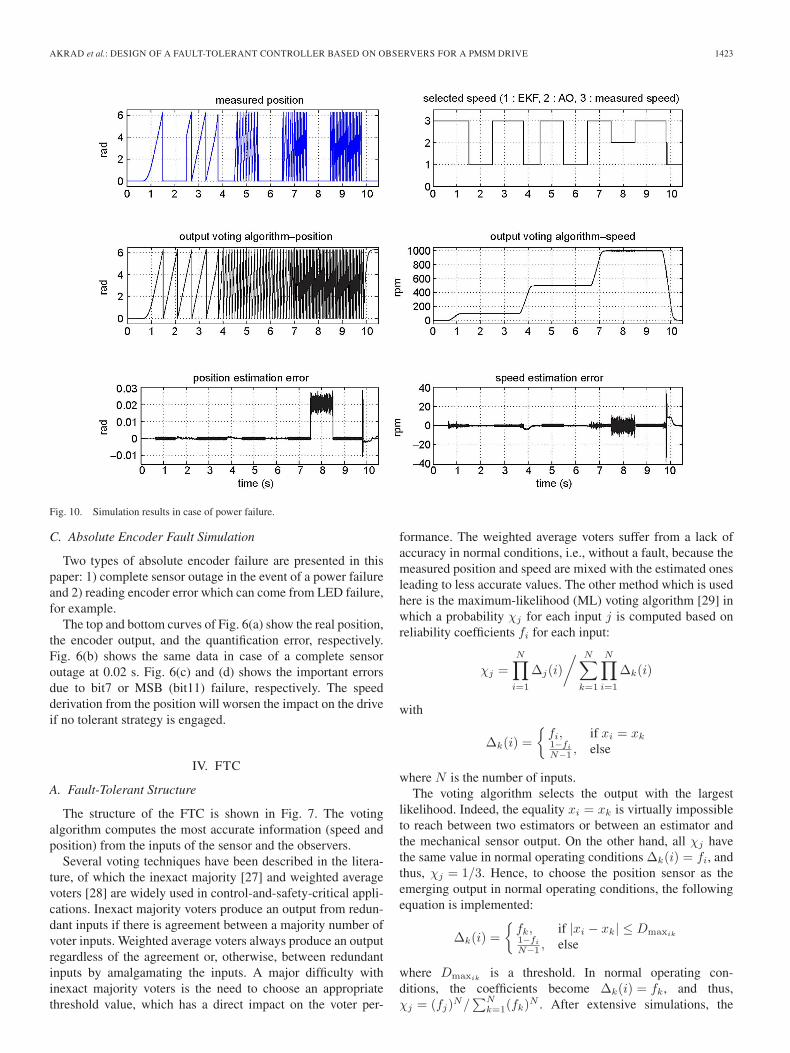
Fig. 10. Simulation results in case of power failure.

C. Absolute Encoder Fault Simulation

Two types of absolute encoder failure are presented in thispaper: 1) complete sensor outage in the event of a power failureand 2) reading encoder error which can come from LED failure,for example.

The top and bottom curves of Fig. 6(a) show the real position,the encoder output, and the quantification error, respectively.Fig. 6(b) shows the same data in case of a complete sensoroutage at 0.02 s. Fig. 6(c) and (d) shows the important errorsdue to bit7 or MSB (bit11) failure, respectively. The speedderivation from the position will worsen the impact on the driveif no tolerant strategy is engaged.

IV. FTC

A. Fault-Tolerant Structure

The structure of the FTC is shown in Fig. 7. The votingalgorithm computes the most accurate information (speed andposition) from the inputs of the sensor and the observers.

Several voting techniques have been described in the litera-ture, of which the inexact majority [27] and weighted averagevoters [28] are widely used in control-and-safety-critical appli-cations. Inexact majority voters produce an output from redun-dant inputs if there is agreement between a majority number ofvoter inputs. Weighted average voters always produce an outputregardless of the agreement or, otherwise, between redundantinputs by amalgamating the inputs. A major difficulty withinexact majority voters is the need to choose an appropriatethreshold value, which has a direct impact on the voter per-

formance. The weighted average voters suffer from a lack ofaccuracy in normal conditions, i.e., without a fault, because themeasured position and speed are mixed with the estimated onesleading to less accurate values. The other method which is usedhere is the maximum-likelihood (ML) voting algorithm [29] inwhich a probability χj for each input j is computed based onreliability coefficients fi for each input:

χj =N∏

i=1

Δj(i)/ N∑

k=1

N∏i=1

Δk(i)

with

Δk(i) ={

fi, if xi = xk1−fi

N−1 , else

where N is the number of inputs.The voting algorithm selects the output with the largest

likelihood. Indeed, the equality xi = xk is virtually impossibleto reach between two estimators or between an estimator andthe mechanical sensor output. On the other hand, all χj havethe same value in normal operating conditions Δk(i) = fi, andthus, χj = 1/3. Hence, to choose the position sensor as theemerging output in normal operating conditions, the followingequation is implemented:

Δk(i) ={

fk, if |xi − xk| ≤ Dmaxik1−fi

N−1 , else

where Dmaxikis a threshold. In normal operating con-

ditions, the coefficients become Δk(i) = fk, and thus,χj = (fj)N/

∑Nk=1(fk)N . After extensive simulations, the


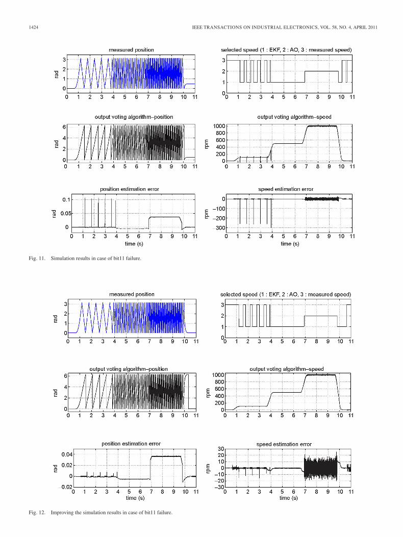
Fig. 11. Simulation results in case of bit11 failure.

Fig. 12. Improving the simulation results in case of bit11 failure.


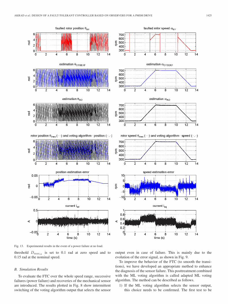
Fig. 13. Experimental results in the event of a power failure at no load.

threshold Dmaxikis set to 0.1 rad at zero speed and to

0.15 rad at the nominal speed.

B. Simulation Results

To evaluate the FTC over the whole speed range, successivefailures (power failure) and recoveries of the mechanical sensorare introduced. The results plotted in Fig. 8 show intermittentswitching of the voting algorithm output that selects the sensor

output even in case of failure. This is mainly due to theevolution of the error signal, as shown in Fig. 9.

To improve the behavior of the FTC (to smooth the transi-tions), we have developed an appropriate method to enhancethe diagnosis of the sensor failure. This posttreatment combinedwith the ML voting algorithm is called adapted ML votingalgorithm. The method can be described as follows.

1) If the ML voting algorithm selects the sensor output,this choice needs to be confirmed. The first test to be


conducted is to determine whether the motor is at stand-still or is starting (actual and estimated speeds are lowerthan predefined thresholds). In that case, the choice isconfirmed. If not, it means that the motor is running ata speed higher than the thresholds, and the algorithmdetermines if there is a complete outage of the sensor(both position and speed outputs are null) or a bit failure(speed signs are different). However, if the former outputof the ML voting algorithm was one of the estimates andin case of sensor recovery, a delay is introduced beforeswitching to the sensor output to avoid violent transients.

2) In the other cases, the tests are conducted to select one ofthe estimators.

This method is evaluated through the simulation of the FTCin case of complete outage of the position sensor. The results inFig. 10 show clearly the improvements compared with thosein Fig. 8, where the adapted ML voting algorithm output isused in the field oriented control (FOC). At low and mediumspeeds, the OTSEKF output is selected in case of failure. Athigh speed, it is the AO output which is engaged to maintain thelevel of performance. The position and speed estimation errorsare evaluated as the difference between the real position andspeed (nonerroneous measured speed) and the emerging outputsof the voting algorithm.

Nevertheless, in case of bit failure (bit11), Fig. 11 showslarge transients in the outputs of the adapted ML voting algo-rithm particularly at low speed. These unsatisfactory results aredue to the rapid variation of the position leading to importantacceleration values when the default appeared. Therefore, tosmooth the evolution, a maximum acceleration threshold γmax

equal to 0.18 rad/s2 is introduced to anticipate the switchingfrom the sensor output to one of the estimators. Fig. 12 showsthe improvement on the speed and position of the drive.

C. Experimental Results

The whole FTC including the adapted ML voting algorithmhas been implemented under Matlab Simulink and downloadedin a dSpace 1103 board. Successive failures (power failure) andrecoveries of the mechanical sensor are introduced between0.93 → 4.93 s and 6.93 → 10.43 s. θmes and ωmes are theactual position and speed. The faults are introduced in theacquisition program, where the faulted position and speed aredenoted as θerr and ωerr, respectively.

Fig. 13 shows the results of the FTC where the outputs ofthe voting algorithm are used in the FOC. For these operatingpoints, it is the OTSEKF that is engaged in the sensorlesscontroller when a position-sensor fault appears. The transitionsbetween the sensor output and the observers are smooth. Theerrors between the estimated and the actual position and speedare good and prove the validity of the FTC. The lower curvesrepresent the stator currents isd and isq , where neither oscilla-tions nor spikes are observed during the switching modes.

V. CONCLUSION

This paper has described a fault-tolerant control system fora high-performance PMSM drive. The FTC is an observer-

based structure with a voting algorithm, which selects theappropriate speed and position in case of mechanical sensorfailure from two observers. A sensorless controller has beenexperimentally evaluated with both observers, the OTSEKF anda back-EMF AO. The transient behavior of both observers havebeen analyzed to extract the reliability coefficients requiredby the maximum-likelihood voting algorithm. The FTC hasbeen improved by developing a new method called adaptedmaximum-likelihood voting algorithm. Finally, the FTC feasi-bility has been experimentally proven in case of an absoluteencoder failure (complete outage) and recovery at low andmedium speed with no load.

The next issues will be the following: 1) the experimentalvalidation of the FTC on the whole torque–speed range, partic-ularly at very low speed where position and speed inobservabil-ities could occur, and 2) the improvement in the tuning of thereliability coefficients based on the evaluation of the modelingerrors.

REFERENCES

[1] K. T. Chau, C. C. Chan, and C. Liu, “Overview of permanent-magnetbrushless drives for electric and hybrid electric vehicles,” IEEE Trans.Ind. Electron., vol. 55, no. 6, pp. 2246–2257, Jun. 2008.

[2] Z. Q. Zhu and D. Howe, “Electrical machines and drives for electric,hybrid, and fuel cell vehicles,” Proc. IEEE, vol. 95, no. 4, pp. 746–765,Apr. 2007.

[3] F. Zidani, D. Diallo, and M. E. H. Benbouzid, “A fuzzy-based approachfor the diagnosis of fault modes in a voltage-fed PWM inverter inductionmotor drive,” IEEE Trans. Ind. Electron., vol. 55, no. 2, pp. 586–593,Feb. 2008.

[4] N. Bianchi, S. Bolognani, and M. D. Pré, “Impact of stator winding of afive-phase permanent-magnet motor on postfault operations,” IEEE Trans.Ind. Electron., vol. 55, no. 5, pp. 1978–1987, May 2008.

[5] Z. Sun, J. Wang, D. Howe, and G. Jewell, “Analytical prediction of theshort-circuit current in fault-tolerant permanent-magnet machines,” IEEETrans. Ind. Electron., vol. 55, no. 12, pp. 4210–4217, Dec. 2008.

[6] D. U. Campos-Delgado, E. Palacios, and D. R. Espinoza-Trejo, “Fault-tolerant control in variable speed drives: A survey,” IET Elect. PowerAppl., vol. 2, no. 2, pp. 121–134, Mar. 2008.

[7] J. Guzinski, M. Diguet, Z. Krzeminski, A. Lewicki, and H. Abu-Rub,“Application of speed and load torque observers in high-speed train drivefor diagnostic purposes,” IEEE Trans. Ind. Electron., vol. 56, no. 1,pp. 248–256, Jan. 2009.

[8] D. Diallo, M. E. H. Benbouzid, and A. Makouf, “A fault-tolerant controlarchitecture for induction motor drives in automotive applications,” IEEETrans. Veh. Technol., vol. 53, no. 6, pp. 1847–1855, Nov. 2004.

[9] Y. S. Jeong, S. K. Sul, S. E. Schulz, and N. R. Patel, “Fault detection andfault-tolerant control of interior permanent-magnet motor drive systemfor electric vehicle,” IEEE Trans. Ind. Appl., vol. 41, no. 1, pp. 46–51,Jan./Feb. 2005.

[10] O. Wallmark, L. Harnefors, and O. Carlson, “Control algorithms for afault-tolerant PMSM drive,” IEEE Trans. Ind. Electron., vol. 54, no. 4,pp. 1973–1980, Aug. 2007.

[11] M. Hilairet, M. E. H. Benbouzid, and D. Diallo, “A self-reconfigurableand fault-tolerant induction motor control architecture for hybrid electricvehicles,” in Proc. IEEE ICEM, Chania, Greece, 2006, pp. 350–356.

[12] S. Y. Kim and I. J. Ha, “A new observer design method for HF signalinjection sensorless control of IPMSMs,” IEEE Trans. Ind. Electron.,vol. 55, no. 6, pp. 2525–2529, Jun. 2008.

[13] A. Piippo, M. Hinkkanen, and J. Luomi, “Analysis of an adaptive observerfor sensorless control of interior permanent magnet synchronous motors,”IEEE Trans. Ind. Electron., vol. 55, no. 2, pp. 570–576, Feb. 2008.

[14] Y. Feng, J. Zheng, X. Yu, and N. V. Truong, “Hybrid terminal sliding-mode observer design method for a permanent-magnet synchronous motorcontrol system,” IEEE Trans. Ind. Electron., vol. 56, no. 9, pp. 3424–3431,Sep. 2009.

[15] G. Zhu, A. Kaddouri, L. A. Dessaint, and O. Akhrif, “A nonlinear stateobserver for the sensorless control of a permanent-magnet ac machine,”IEEE Trans. Ind. Electron., vol. 48, no. 6, pp. 1098–1108, Dec. 2001.


[16] P. P. Vas, Sensorless Vector and Direct Torque Control. London, U.K.:Oxford Univ. Press, 1998.

[17] E. Laroche, E. Sedda, and C. Durieu, “Methodological insights for onlineestimation of induction motor parameters,” IEEE Trans. Control Syst.Technol., vol. 16, no. 5, pp. 1021–1028, Sep. 2008.

[18] M. S. Grewal and A. P. Andrews, Kalman Filtering, Theory and Practice.Englewood Cliffs, NJ: Prentice-Hall, 1993.

[19] C. S. Hsieh and F. C. Chen, “Optimal solution of the two-stage Kalmanestimator,” IEEE Trans. Autom. Control, vol. 44, no. 1, pp. 194–199,Jan. 1999.

[20] A. Akrad, M. Hilairet, and D. Diallo, “A sensorless PMSM drive using atwo stage extended Kalman estimator,” in Proc. IEEE IECON, Orlando,FL, 2008, pp. 2776–2781.

[21] M. Hilairet, F. Auger, and E. Berthelot, “Speed and rotor flux estimationof induction machines using a two-stage extended Kalman filter,” Auto-matica, vol. 45, no. 8, pp. 1819–1827, Aug. 2009.

[22] Z. Chen, M. Tomita, S. Doki, and S. Okuma, “An extended electromotiveforce model for sensorless control of interior permanent magnet synchro-nous motors,” IEEE Trans. Ind. Electron., vol. 50, no. 2, pp. 288–295,Apr. 2003.

[23] B. Nahid-Mobarakeh, F. Meibody-Tabar, and F. Sargos, “Mechanical sen-sorless control of PMSM with online estimation of stator resistance,”IEEE Trans. Ind. Appl., vol. 40, no. 2, pp. 457–471, Mar./Apr. 2004.

[24] Z. Boulbair, M. Hilairet, F. Auger, and L. Loron, “Sensorless controlof a PMSM using an efficient extended Kalman filter,” in Proc. ICEM,Cracovie, Pologne, 2004, p. 637.

[25] W. Levine, The Control Handbook. Boca Raton, FL: CRC.[26] C. W. De Silva, Mechatronics: An Integrated Approach. Boca Raton, FL:

CRC, 2005.[27] J. M. Bass, P. R. Croll, P. J. Fleming, and L. J. C. Woolliscroft, “Three

domain voting in real-time distributed control systems,” in Proc. 2ndEuromicro Workshop Parallel Distrib. Process., 1994, pp. 317–324.

[28] G. Latif-Shabgahi, J. M. Bass, and S. Bennett, “History-based weightedaverage voter: A novel software voting algorithm for fault-tolerantcomputer systems,” in Proc. 9th Euromicro Workshop Parallel Distrib.Process., 2001, pp. 402–409.

[29] Y. Leung, “Maximum likelihood voting for fault-tolerant software withfinite output-space,” IEEE Trans. Rel., vol. 14, no. 3, pp. 419–427,Sep. 1995.

Ahmad Akrad was born in Damascus, Syria, in1977. He received the B.Sc. degree in electricaland electronic engineering from the University ofAleppo, Aleppo, Syria, in 2001 and the M.Sc. degreein automatic and signal processing and the Ph.D.degree in electrical engineering from the Universityof Paris 11, Orsay Cedex, France, in 2006 and 2010,respectively.

He is currently with the Laboratoire de GénieElectrique de Paris/SPEE-Labs, CNRS–ÉcoleSupérieure d’Électricité (SUPELEC)–Université

Pierre et Marie Curie P6–Université Paris-Sud 11, Gif-sur-Yvette, France.His main research interests are drive control and fault diagnosis of electricmachines.

Mickaël Hilairet (M’08) was born in Les Sablesd’Olonne, France, in 1973. He received the Electricalengineering degree from the Ecole des Hautes EtudesIndustrielles de Lille, Lille, France, in 1997, theM.Sc. degree in electrical engineering from the Na-tional Polytechnic Institute of Toulouse, Toulouse,France, in 1998, and the Ph.D. degree in electricalengineering from the University of Nantes, Saint-Nazaire, France, in 2001.

From 2001 to 2003, he was an Engineer withThalès Communication (CHOLET) and Geral (BEL-

LEY), France. In 2003, he joined South Brittany University, Lorient, France,as an Assistant Professor, and in 2004, he joined the Institut Universitairede Technologie of Cachan, Université Paris-Sud 11, France, as an AssociateProfessor of electrical and computer engineering. He is with the Laboratoire deGénie Electrique de Paris, Gif-sur-Yvette, France. His main research interestsare drive control, estimation, fault diagnosis of electric machines, and fuel-cellcontrol.

Demba Diallo (M’99–SM’05) received the M.Sc.and Ph.D. degrees in electrical and computer en-gineering from the National Polytechnic Instituteof Grenoble, Grenoble, France, in 1990 and 1993,respectively.

After graduation, from 1994 to 1999, hewas a Research Engineer with the Laboratoired’Electrotechnique de Grenoble, France, onelectrical drives and active filters. In 1999, he joinedthe University of Picardie “Jules Verne,” Amiens,France, as an Associate Professor of electrical

engineering. Since September 2004, he has been with the Institut Universitairede Technologie of Cachan, University of Paris-Sud 11, Orsay, France, andthe Laboratoire de Génie Electrique de Paris, Gif-sur-Yvette, France, as anAssociate Professor of electrical engineering. He is currently a Full Professor.His current area of research includes advanced control techniques anddiagnosis of ac drives, renewable energies, design of electric powertrains, andautonomous systems.

Dr. Diallo is an Associate Editor of the IEEE TRANSACTIONS ON VEHIC-ULAR TECHNOLOGY.

Design of a fault-tolerant controller based on observers for a PMSM drive

Documents

Transcript of Design of a fault-tolerant controller based on observers for a PMSM drive