Performance Analysis of Kernel Adaptive Filters based on LMS Algorithm

Procedia Computer Science 20 ( 2013 ) 39 – 45

1877-0509 © 2013 The Authors. Published by Elsevier B.V.Selection and peer-review under responsibility of Missouri University of Science and Technologydoi: 10.1016/j.procs.2013.09.236

ScienceDirect

Abstract

1. Introduction

Available online at www.sciencedirect.com

© 2013 The Authors. Published by Elsevier B.V.Selection and peer-review under responsibility of Missouri University of Science and Technology

40 Ibtissam Constantin and Régis Lengellé / Procedia Computer Science 20 ( 2013 ) 39 – 45

2. Principles of kernel-based optimal filtering in RKHS

(. )

<. , .>(. , ), ( ) =< , (. , ) > ,(. ) (. , ) ( , ) =< (. , ), (. , ) >, (. , . ){ (. , ), } (. )(. ) (. , ) ( , ) =< ( ), ( ) >(. )( , ) ( ) ( ) 0( ) <( , ) = ( 2 ) ( , ) = ( +< , >) 0

(. ) ( ) =<(. ), (. , ) > min ( ( )) (4)(. )(. ) = (. , )


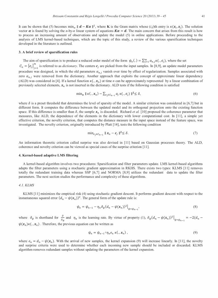
It can be shown that (5) becomes min , where K is the Gram matrix whose ( , )th entry is ( , ). The solution vector is found by solving the -by- linear system of equations = . The main concern that arises from this result is how to process an increasing amount of observations and update the model (5) in online applications. Before proceeding to the analysis of LMS kernel-based techniques, which are the topic of this study, a review of the various sparsification techniques developed in the literature is outlined.

3. A brief review of sparsification rules

The aim of sparsification is to produce a reduced order model of the form (. ) = , (. , ), where the set = is referred to as . The centers are picked from the input samples. In [8,9], an update model parameters procedure was designed, in which the old parameters , vanish over time by effect of regularization. Samples associated with zero , were removed from the dictionary. Another approach that exploits the concept of approximate linear dependency (ALD) was considered in [4]. If a kernel function (. , ) at time can be approximately represented by a linear combination of previously selected elements, is not inserted in the dictionary. ALD tests if the following condition is satisfied

min (. , ) (. , ) , (6) where is a preset threshold that determines the level of sparsity of the model. A similar criterion was considered in [6,7] but in different form. It computes the difference between the updated model and its orthogonal projection onto the existing function space. If this difference is smaller than , the sample is discarded. Richard [10] proposed the coherence parameter that measures, like ALD, the dependence of the elements in the dictionary with lower computational cost. In [11], a simple yet effective criterion, the novelty criterion, that computes the distance measure in the input space instead of the feature space, was investigated. The novelty criterion, originally introduced by Platt [14], tests the following condition min . (7) An information theoretic criterion called surprise was also devised in [11] based on Gaussian processes theory. The ALD, coherence and novelty criterion can be viewed as special cases of the surprise criterion [11].

4. Kernel-based adaptive LMS filtering

A kernel-based algorithm involves two procedures: Sparsification and filter parameters update. LMS kernel-based algorithms adapts the filter parameters using a stochastic gradient approximation in RKHS. There exists two types: KLMS [11] removes totally the redundant training data whereas SSP [6,7] and NORMA [8,9] utilizes the redundant data to update the filter parameters. The next section studies the performance and complexity of these algorithms.

KLMS [11] minimizes the empirical risk (4) using stochastic gradient descent. It performs gradient descent with respect to the instantaneous squared error ( ( )) . The general form of the update rule is: = ( ( )) , (8) where is shorthand for and is the learning rate. By virtue of property (1), ( ( )) = 2(( ) (. , ) . Therefore, the previous equation can be written as = + (. , ) , (9) where = ( ). With the arrival of new samples, the kernel expansion (9) will increase linearly. In [11], the novelty and surprise criteria were used to determine whether each incoming new sample should be included or discarded. KLMS algorithm removes redundant samples without updating the parameters of the kernel expansion.


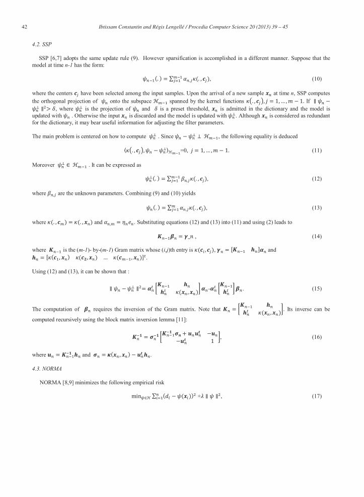
SSP [6,7] adopts the same update rule (9). However sparsification is accomplished in a different manner. Suppose that the model at time has the form: (. ) = , (. , ), (10) where the centers have been selected among the input samples. Upon the arrival of a new sample at time , SSP computes the orthogonal projection of onto the subspace spanned by the kernel functions . , , = 1,… , 1. If > , where is the projection of and is a preset threshold, is admitted in the dictionary and the model is updated with . Otherwise the input is discarded and the model is updated with . Although is considered as redundant for the dictionary, it may bear useful information for adjusting the filter parameters. The main problem is centered on how to compute . Since , the following equality is deduced . , , =0, = 1,… , 1. (11) Moreover . It can be expressed as (. ) = , (. , ), (12) where , are the unknown parameters. Combining (9) and (10) yields (. ) = , (. , ), (13) where (. , ) = (. , ) and , = . Substituting equations (12) and (13) into (11) and using (2) leads to = _ , (14) where is the ( )- by-( ) Gram matrix whose ( , )th entry is ( , ), = [ ] and = [ ( , ) ( , ) … ( , )] . Using (12) and (13), it can be shown that :

= ( , ) - . (15)

The computation of requires the inversion of the Gram matrix. Note that = ( , ) . Its inverse can be

computed recursively using the block matrix inversion lemma [11]:

= + 1 , (16)

where = and = ( , ) .

NORMA [8,9] minimizes the following empirical risk min ( ( )) + , (17)


where a regularization parameter has been added in order to prevent the algorithm from overfitting the data. As KLMS and SSP, NORMA performs stochastic gradient descent with respect to the instantaneous risk ( ( )) + . The gradient is defined as ( ( )) + = 2( ( ) (. , ) + 2 , which leads to the following update rule = (1 ) + (. , ). (18) At each iteration, a kernel function is inserted and the parameters of the previous model are truncated by (1 ). Sparsity is achieved by dropping small coefficients.

Among the three algorithms, SSP has the highest computation cost. The sparsification procedure in SSP requires the inversion of the kernel matrix which is performed with operations. The complexity of the parameter update is . This leads to an overall complexity of . The complexity of KLMS is clearly lower than SSP if an appropriate sparsification criterion to build the dictionary is chosen. For instance, the novelty criterion may be selected which requires arithmetic operations The adjustment of the model parameters, which is only accomplished when a new sample is inserted in the dictionary has complexity. However, as it will be seen in the experimental section, the size of the kernel expansion in SSP is significantly lower than KLMS. It never exceeds a few tens. NORMA is an algorithm. The experimental section shows that the use of even small values of the regularization parameter degrades the performance of the algorithm when compared to KLMS and SSP. The size of the kernel expansion in NORMA is equal to the size of the training data.

5. Experiments

Experiments were conducted on simulated and real data to compare the performance of the proposed techniques. The Gaussian kernel was considered in all the experiments. The enhanced novelty criterion was used for KLMS algorithm [11]. It tests first if the condition (7) is verified. If it is, the input sample is discarded. Otherwise it tests if the prediction error exceeds a threshold . If this condition is met, the input sample is accepted as a new center.

The first application consists of predicting the highly nonlinear time series [15]

= (0.8 0.5 exp( )) (0.3 + 0.9 exp( )) +0.1sin( )). (19)

The data were generated by iterating the above equation from the initial conditions (0.1,0.1). Output was corrupted by an additive zero-mean white Gaussian noise with variance . Different realizations of the noise were considered as depicted in table 1. The time embedding were chosen as 2, i.e, = [ ] was used as the input to predict . A variable step size parameter was used that is updated according to [16]

= + , (20)

where 0 < < 1 and > 0 , and is set to and when it falls below or above these bounds. This step size induced better performance than a fixed step size. As can be seen from (20), a large prediction error increases the step size to provide faster tracking. If the prediction error decreases, the step size will be decreased to reduce the misadjustment. Preliminary experiments yielded = 0.99, = 0.001, = 0.01, and = 1. A test set of 100 sequences of 4000 samples was constituted and the performance of the algorithms was measured in steady state by evaluating the normalized mean-square error (NMSE) over the last 1000 samples of each sequence, namely

( ( )) , (21)

where is the variance of the desired output in the selected interval. The optimum parameters setting was determined by cross-validation. The parameters and were chosen by grid search over (10 10 ) × (10 10 ) with increment 2 × 10 within each range [10 10 ]. The kernel parameter was varied from 0.1 to 0.9 in increments of 0.05. 25 sequences of 4000 samples were generated and the average NMSE was computed on the last 1000 samples for each combination of ( , , ). It was observed that the regularization parameter deteriorates the performance of NORMA compared to SSP and KLMS and therefore was set to 0. Table 1 reports the average NMSE and the average dictionary size on the test set for different noise variances . It shows that the three methods exhibit comparable performances, with a slight advantage for KLMS. However, in terms of sparsity, NORMA and KLMS require significantly higher number of centers than SSP. This could be expected since the regularization parameter in Norma is equal to 0 and that KLMS removes totally the redundant training data. KLMS included most of the training samples in the dictionary because they are needed in the parameter update. Figure 1


0 500 1000 1500 2000 2500 3000 3500 400010

-1.9

10-1.8

10-1.7

10-1.6

10-1.5

10-1.4

10-1.3

KLMS

SSPNORMA

displays the learning curves for = 0.01. The three methods have similar convergence rates, requiring about 500 iterations to converge.

Table 1. NMSE and dictionary size for different realizations of the noise, averaged on 100 sequences.

KLMS SSP NORMA NMSE Dictionary size NMSE Dictionary size NMSE Dictionary size

0.5 0.158 1280.8 0.160 72.99 0.160 4000 0.1 0.035 1826 0.036 33.78 0.036 4000

0.06 0.0136 976.12 0.0138 31.19 0.0138 4000

Fig.1. Learning curves for KLMS, SSP and NORMA obtained by averaging over 100 experiments.

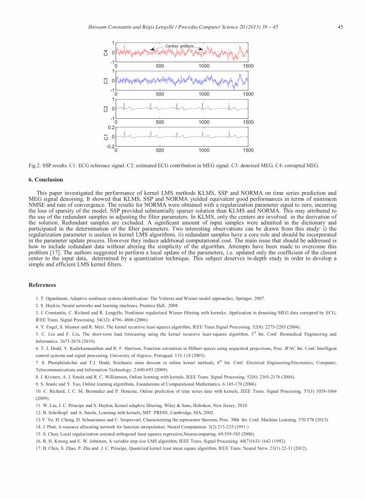
As a second application, KLMS, SSP and NORMA were applied on magnetoencaphalographic (MEG) data corrupted by cardiac artifacts. The recorded electocardiographic (ECG) signal was used as the reference signal. The MEG signal was used as the desired output so the residue is the denoised MEG signal. NMSE was used as a measure of performance. A variable step size parameter was selected that obeys the same update rule (20). After trial and error, the values = 0.998, = 0.00005, =0.0001, and = 0.9 were selected. The optimum parameters , and were determined by cross-validation as previously by performing a grid search over (10 10 ) × (10 10 ) × (10 1) with increment 2 × 10 within each range [10 10 ] for and and 5× 10 for . The dimension of the input vector was varied from 2 to 13. Here again, the regularization parameter was set to 0. KLMS, SSP and NORMA were tested on 10 independent sequences of 10000 samples and NMSE was computed on the last 4000 samples of each sequences. Table 2 summarizes the results, averaged over the 10 independent trials. We notice that SSP produced a much sparser model than KLMS and NORMA with equivalent performance. Figure 2 presents SSP results for one trial, where =11, = 0.15 and = 0.0003. The highest two curves show the contaminated and denoised MEG signals. Curves C1 and C2 show the ECG reference channel and the estimated artifact signal.

Table 2. NMSE and dictionary size obtained with MEG data averaged on 10 sequences.

Algorithm NMSE Dictionary size KLMS 0.853 9186.2

SSP 0.854 16.8 NORMA 0.856 10000


Fig.2. SSP results. C1: ECG reference signal. C2: estimated ECG contribution in MEG signal. C3: denoised MEG. C4: corrupted MEG.

6. Conclusion

This paper investigated the performance of kernel LMS methods KLMS, SSP and NORMA on time series prediction and MEG signal denoising. It showed that KLMS, SSP and NORMA yielded equivalent good performances in terms of minimum NMSE and rate of convergence. The results for NORMA were obtained with a regularization parameter equal to zero, incurring the loss of sparsity of the model. SSP provided substantially sparser solution than KLMS and NORMA. This may attributed to the use of the redundant samples in adjusting the filter parameters. In KLMS, only the centers are involved in the derivation of the solution. Redundant samples are excluded. A significant amount of input samples were admitted in the dictionary and participated in the determination of the filter parameters. Two interesting observations can be drawn from this study: i) the regularization parameter is useless in kernel LMS algorithms. ii) redundant samples have a core role and should be incorporated in the parameter update process. However they induce additional computational cost. The main issue that should be addressed is how to include redundant data without altering the simplicity of the algorithm. Attempts have been made to overcome this problem [17]. The authors suggested to perform a local update of the parameters, i.e. updated only the coefficient of the closest center to the input data, determined by a quantization technique. This subject deserves in-depth study in order to develop a simple and efficient LMS kernel filters.

References

1. T. Ogunfunmi, Adaptive nonlinear system identification: The Volterra and Wiener model approaches, Springer, 2007. 2. S. Haykin, Neural networks and learning machines, Prentice Hall, 2008. 3. I. Constantin, C. Richard and R. Lengelle, Nonlinear regularized Wiener filtering with kerneks: Application in denoising MEG data corrupted by ECG, IEEE Trans. Signal Processing. 54(12): 4796- 4806 (2006). 4. Y. Engel, S. Mannor and R. Meir, The kernel recursive least squares algorithm, IEEE Trans.Signal Processing. 52(8): 2275-2285 (2004). 5. C. Liu and F. Liu, The short-term load forecasting using the kernel recursive least-squares algorithm, 3rd Int. Conf. Biomedical Engineering and Informatics. 2673-2676 (2010). 6. T. J. Dodd, V. Kadirkamanathan and R. F. Harrison, Function estimation in Hilbert spaces using sequential projections, Proc. IFAC Int. Conf. Intelligent control systems and signal processing, University of Algrave, Portugual. 113-118 (2003). 7. S. Phonphitakchai and T.J. Dodd, Stochastic meta descent in online kernel methods, 6th Int. Conf. Electrical Engineering/Electronics, Computer, Telecommunications and Information Technology. 2:690-693 (2009). 8. J. Kivinen, A. J. Smola and R. C. Williamson, Online learning with kernels, IEEE Trans. Signal Processing. 52(8): 2165-2176 (2004). 9. S. Smale and Y. Yao, Online learning algorithms, Foundations of Computational Mathematics. 6:145-170 (2006). 10. C. Richard, J. C. M. Bermudez and P. Honeine, Online prediction of time series data with kernels, IEEE Trans. Signal Processing. 57(3) 1058-1066 (2009). 11. W. Liu, J. C. Principe and S. Haykin, Kernel adaptive filtering, Wiley & Sons, Hoboken, New Jersey, 2010. 12. B. Scholkopf and A. Smola, Learning with kernels, MIT PRESS, Cambridge, MA, 2002. 13.Y. Yu, H. Cheng, D. Schuurmans and C. Szepesvari, Characterizing the representer theoerm, Proc. 30th Int. Conf. Machine Learning. 570-578 (2013). 14. J. Platt, A resource allocating network for function interpolation, Neural Computation. 3(2) 213-225 (1991.) 15. S. Chen, Local regularization assisted orthogonal least squares regression,Neurocomputing. 69:559-585 (2006). 16. R. H. Kwong and E. W. Johnston, A variable step size LMS algorithm, IEEE Trans. Signal Processing. 40(7)1633-1642 (1992). 17. B. Chen, S. Zhao, P. Zhu and J. C. Principe, Quantized kernel least mean square algorithm, IEEE Trans. Neural Netw. 23(1) 22-31 (2012).

0 500 1000 1500-1

0

1

C4

0 500 1000 1500-1

0

1

C3

0 500 1000 1500-1

0

1C

2

0 500 1000 1500-0.2

0

0.2

C1

Cardiac artifacts

Performance Analysis of Kernel Adaptive Filters based on LMS Algorithm

Documents

Transcript of Performance Analysis of Kernel Adaptive Filters based on LMS Algorithm