IMPLEMENTATION OF INTERFERENCE CANCELLATION BY ADAPTIVE FILTERS

[Arun*, 4(3): March, 2015] ISSN: 2277-9655

Scientific Journal Impact Factor: 3.449

(ISRA), Impact Factor: 2.114

http: // www.ijesrt.com© International Journal of Engineering Sciences & Research Technology

[292]

IJESRT INTERNATIONAL JOURNAL OF ENGINEERING SCIENCES & RESEARCH

TECHNOLOGY

IMPLEMENTATION OF INTERFERENCE CANCELLATION BY ADAPTIVE

FILTERS Arun.C*, Veena V S

*Assistant Professor, Department of ECE, Collage of Engineering Perumon,Kollam,Kerala,India

Assistant Professor, Department of EEE, Collage of Engineering Perumon,Kollam,Kerala,India

ABSTRACT This paper investigates on the development and implementation of adaptive noise cancellation (ANC) algorithm

meant for mitigating the high machinery noise in factory plants ,which makes the speech signal unintelligible.This

opens up the need for an adaptive filter that cancels this interference of noise.An adaptive filter is computational

device that attempts to model the relationship between two signals in real time in an iterative manner.An adaptive

filter self adjusts the filter coefficients according to an adaptive algoritm.A comparative study of Gradient based

adaptive Infinite Impulse Response(IIR) algorithm and its modified version is performed using MATLAB simulator

interms of converging speed.From the simulation result the best IIR algorithm is used for implementation in

Performance Optimized with Enhanced RISC PC ( Power PC) 7448.

KEYWORDS: Adaptive noise cancellation (ANC),IIR filter,Power PC 7448,Adaptive Line Enhancer(ALE),Mean

square error (MSE)

INTRODUCTION In the field of signal processing, there is a significant

need for a special class of digital filters known as

adaptive filters. Adaptive filters are used commonly

in many different configurations, and for certain

applications these filters have a great advantage over

the standard digital filters. They can change their

filter coefficients according to preset rules. An

adaptive filter is a digital filter that can adjust its

coefficients to give the best match to a given desired

signal[1]. When an adaptive filter operates in a

changeable environment the filter coefficients can

adapt in response to changes in the applied input

signals. Based on recursive algorithms adaptive

filters update their coefficients and train them to

reach the optimum solution. Adaptive filters are

mainly used in applications like system identification,

linear prediction, inverse system identification, noise

cancellation etc[6]. Adaptive signal processing is one

of the most important classes of algorithms for

modern communication systems. The concept of

adaptive noise cancellation has become widespread

in the areas of communications and signal

processing. The noise-cancellation problem involves

two received signals, commonly referred to as the

primary and the reference. The goal is to cancel (that

is, subtract out) the portions of the two signals that

are mutually correlated [2].

There are different adaptive algorithms (eg. Least

Mean Square(LMS), Normalized Least Mean Square

(NLMS) etc.) that can be used in time domain. Some

widely used methods with Adaptive FIR filter have

been explained by S. Haykins [6] & B.Widrow [7].

FIR filters are more stable than IIR filters.Adaptive

filters are attractive: many fewer coefficients may be

needed to achieve the desired performance in some

applications[3]. However, it is more difficult to

develop stable IIR algorithms, they can converge

slowly. Adaptive IIR algorithms are used in some

applications (such as low frequency noise

cancellation) where the need for IIR-type responses is

great. In some cases, the exact algorithm used by a

company is a tightly guarded trade secret.However a

gradient-based Adaptive IIR algorithm, with some

additional features that enable it to adapt more

quickly is explained by Don R.Hush [2]. A modified

version of the above algorithm gives even faster

http://www.ijesrt.com/

[Arun*, 4(3): March, 2015] ISSN: 2277-9655




[293]

convergence. So the modified algorithm can be used

for implementation.

ADAPTIVE SIGNAL PROCESSING The term Adaptive can be understood by considering

a system which is trying to adjust itself so as to

respond to some phenomenon that is taking place in

its surroundings.This is what adaptation means.

Moreover there is a need to have a set of steps or

certain procedure called algorithm by which this

process of adaptation is carried out[4] .

Figure:1 Basic adaptive filter structure

The adaptive filter structure shown in the figure 1in

which the filter’s output y is compared with a desired

signal d to produce an error signal e, which is fed

back to the adaptive filter. The error signal is given as

input to the adaptive algorithm, which adjusts the

variable filter to satisfy some predetermined rules. In

stochastic frame work (based on Wiener filter

theory), the optimum coefficients of a linear filter are

obtained by minimization of its mean-square error

(MSE). All the adaptive algorithms take the output

error of the filter, correlate that with the samples of

filter input in some way, and use the result in a

recursive equation to adjust the filter coefficients

iteratively

ADAPTIVE ALGORITHMS There are many adaptive algorithms available. Two

main algorithms are LMS and NLMS algorithms[7]..

Least Mean Square Algorithm (LMS)

The LMS algorithm is one of the most widely used

adaptive filtering algorithms due to its simplicity and

robustness to signal statistics. LMS algorithm uses

the instantaneous value of the square of the error

signal as an estimate of the MSE.

Figure:2 An N tap transversal adaptive filter[8]

Figure 2 depicts an N-tap transversal adaptive filter.

The filter input, x (n), desired output, d (n) and the

filter output,

The equations are derived inline with[8]

y (n) = )()(1

0

inxnwN

i

i

(1)

are assumed to be real-valued sequences. The tap

weights w0 (n), w1 (n) ... ,wN-1(n) are selected so that

the difference (error),

e(n)=d(n)-y(n) (2)

is minimized in some sense.

It may be noted that the filter tap weights are

explicitly indicated to be functions of the time index

'n'. The LMS algorithm changes (adapts) the filter tap

weights so that e(n) is minimized in the mean-square

sense, thus the name least mean square. It is a

sequential algorithm which can be used to adapt the

tap weights of a filter by continuous observation of

its input, x(n), and desired output, d(n).

The recursive weight update equation is given by

w(n+1) = w(n) - µ e2(n) (3)

Where w(n) = [w0(n) w1(n) ............wN-1(n)]T

, µ

is the algorithm step-size parameter and is the

gradient operator .

e2(n) = -2e(n)x(n) (4)

Where x(n) = [x(n) x(n-1) ... x(n-N+1)] T

.

Substituting the result in equation (3)

w(n+1) = w(n)+2 µ e(n)x(n). (5)

This is referred to as the LMS recursion. It suggests a

simple procedure for recursive adaptation of the filter

coefficients after the arrival of every new input

sample, x(n), and its corresponding desired output

sample, d(n).


[Arun*, 4(3): March, 2015] ISSN: 2277-9655




[294]

Normalized Least Mean Square Algorithm

(NLMS)

The normalized (NLMS) algorithm may be viewed as

a special implementation of the LMS algorithm

which takes into account the variation in the signal

level at the filter input and selects a normalized step

size parameter which results in a stable as well as fast

converging adaptation algorithm. NLMS algorithm

provides optimized performance keeping the

stability. The only difference of NLMS algorithm

with that of LMS algorithm is that the step size

adjusts based on the input signal, thereby converging

faster than LMS algorithm.

Consider the LMS recursion

w(n+1) = w(n)+2 µ e(n)x(n). (6)

But the step size µ changes based on input x(n) such

that

µ = )()(2

1

nn Txx (7)

Substitute the value in equation (6)

w(n+1) = w(n)+)()(

1

nnT xx e(n)x(n). (8)

This is the NLMS recursion. When this is combined

with the filtering equation (1) and the error

estimation equation (2) NLMS algorithm is obtained.

ADAPTIVE NOISE CANCELLATION The ANC method uses a “primary” input containing

the corrupted signal and a “reference” input

containing noise correlated in some unknown way

with the primary noise. The reference input is

adaptively filtered and subtracted from the primary

input to obtain the signal estimate.

Figure:3 Adaptive noise cancelling concept

A signal s is transmitted over a channel to a sensor

that also receives a noise n0 uncorrelated with the

signal. The combined signal and noise s+ n0 form

the primary input to the canceller. A second sensor

receives a noise n1 uncorrelated with the signal but

correlated in some unknown way with the noise n0.

This sensor provides the reference input to the

canceller. The noise n1 is filtered to produce an

output y that is as close a replica as possible of n0.

This output is subtracted from the primary input s+

n0 to produce the system output z=. s+ n0 -y Hence

the output of the system contains the signal alone. Adaptive noise cancellation has been used for several

applications like cancelling the Maternal ECG in

Fetal Electrocardiography,Cancelling noise in speech

signals,Cancelling periodic interference without an

external reference source.

ADAPTIVE NOISE CANCELLATION

USING FIR FILTER In adaptive noise cancellation an adaptive filter is

used to determine the relationship between the noise

reference signal x(n) and the component of this noise

that is contained in the measured signal(desired) d(n).

After subtracting out this component adaptively the

error signal e(n) gives the signal of interest. Hence

adaptive noise cancellation is a method of estimating

signals corrupted by additive noise or interference.

Figure:4 Adaptive filter as a noise canceller[9]

Simulation Results

For simulation sinusoidal signal is taken as the pure

signal. Then add noise with this pure signal. Adaptive

noise cancellation is performed using above

algorithms and compare the performance of

algorithms. Figure 4 shows the pure sinusoidal signal,

figure 5 shows the noise which is added to the pure

signal to make the noise corrupted signal. The

sinusoidal signal is distorted by the addition of noise.

The noise corrupted signal is shown in figure 6.


[Arun*, 4(3): March, 2015] ISSN: 2277-9655




[295]

Figure:5 Pure sinusoidal signal

Figure:5 Noise Signal

Figure:6 Noise corrupted signal

The noise filtered signals (nfs) obtained using the

two algorithms shown in the figures below.

Figure:7 Noise filtered signal using LMS algorithm

Figure:8 Noise filtered signal using NLMS algorithm

The figure 7 and 8 show noise filtered signals using

LMS and NLMS algorithms respectively. From the

simulation result it is clear that using the adaptive

algorithms the signal can be recovered. The NLMS

algorithm converges faster than the conventional

LMS algorithm

ADAPTIVE LINE ENHANCER USING IIR

STRUCTURE

The Adaptive Line Enhancer enhances the sinusoidal

component of the reference input so that output has

high signal to noise ratio SNR. From the ALE we

also obtain an estimate of the sinusoidal frequency.

This ALE can be utilizes as noise canceller. Several

forms of the ALE are available. The most popular is

the FIR ALE. It has the advantage of being inherently

stable and easy to adapt. However, it often requires a


[Arun*, 4(3): March, 2015] ISSN: 2277-9655




[296]

large number of filter weights to provide adequate

enhancement of narrow-band signals. In an effort to

reduce the number of weights, several forms of

adaptive recursive filters (IIR) can be used.

Figure:9 Adaptive Line Enhancer[2]

The purpose of is to decorrelate the input noise

and its delayed version present at the filter input. This

causes the adaptive process to respond only to the

sinusoid. As such, H (z) forms a band pass filter

around the sinusoid, applying at the same time a

phase shift to compensate for the delay so that the

sinusoidal component of xk is removed at the

summer. At the output of the adaptive filter x’k,, the

enhanced sinusoid is obtained. To simplify the

analysis assume nk is white noise so that = 1 is

sufficient for decorrelation.

GRADIENT BASED ADAPTIVE

ALGORITHM FOR IIR ALE The technique used here is a gradient-based

algorithm with some additional features that enable it

to adapt more quickly. The filter output is given by

'

kx = }1

1{

2

2

r

r

kw 1kx - 2

2 )1( kxr + '

1kk xw

- '

2

2

kxr (9)

Where 0<< r <1

-2r<w<2r, r is the radius of

the circle just inside the unit circle Also from figure 9, the error output is defined to be

'

kkk xx (10)

The coefficient update for the adaptive algorithm can

be expressed as

kkkk ww 1 (11)

Where ρ is a parameter which controls the rate of

convergence,ɛk is the error, and αk is the partial

derivative

k

k

kw

x

'

(12)

From (9) and the definition of (11) , recursive

relationship for αk

'

112

2

2

2

1 )1

1(

kkkkkk xx

r

rrw (13)

The coefficient update is then defined by

(10),(11) and (13). The normalization factor is incorporated by

reexpressing the coefficient update in (11) as

k

kk

kk ww

11 (14)

Where k and k are as defined above and

2

1 )1( kkk vv (15)

The “forgetting factor “v is in the range 0<<v<1 The performance of this algorithm can be

enhanced even further by using an approximate

partial derivative in place of αk in (13). The modified

derivative, denoted by αmk,is obtained from (13) by

suppressing the recursive terms, i.e.,

'

112

2

)1

1(

kkmk xx

r

r (16)

The resulting algorithm is then defined by the same

set of equations as before, with αk replaced by αmk.

The effect of this modification is to produce a

modified gradient estimate which has a higher

probability of taking on the correct sign (direction)

than the true gradient. This in turn leads to a faster

convergence rate.

Simulation Results

After performing the adaptive process, at the output

of the filter we get the enhanced version of the

sinusoid. At the output of the summer, (error signal)

sinusoidal component of input is removed. The

simulation result shows the Power Spectral Density

(PSD) of pure signal, noise corrupted signal,

comparisons of PSD of error signals and enhanced

signals using both the algorithms. Mean Square Error

(MSE) of two algorithms is also shown.


[Arun*, 4(3): March, 2015] ISSN: 2277-9655




[297]

Figure:10 PSD of pure signal

Figure:11 PSD of noise corrupted signal

Figure:12 Comparison of PSDof error

Figure:13 Comparison of PSD of enhanced signal

Figure:14 Comparison of Mean square error

From the PSD of error signal it is clear that a very

large reduction of power occur at the output of the

summer. The modified algorithm provides more

reduction in power. The figure 15 shows the

reduction in power for different Signal to Noise Ratio

(SNR) with both algorithms. The figure 16 shows the

convergence time of both the algorithms.

Figure:15 Reduction of Power in db

Figure:16 Comparison of convergence time


[Arun*, 4(3): March, 2015] ISSN: 2277-9655




[298]

ADAPTIVE IIR NOISE CANCELLATION

ALE can be utilized as noise canceller with

experimental data. ALE is used as the basic structure

for noise cancellation.

Figure:17 IIR noise canceller

Here the input signal X contains the speech signal

and sinusoidal noise. The purpose of Δ is to

decorrelate the input speech and its delayed version

present at the filter input. This causes the adaptive

process to respond only to the sinusoid As such, H (z)

forms a band pass filter around the sinusoid, applying

at the same time a phase shift to compensate for the

delay so that the sinusoidal component of X is

removed at the summer. By taking the

autocorrelation of speech signal one can find out

suitable value for Δ.So at the output of the summer

(error signal) contains the speech alone. i.e., the

sinusoidal noise is adaptively cancelled out. Let the

signal to be interfered with noise such that the SNR is

controllable and verify the performance of IIR

structure in highly noise environment. The system is

provided with the permission to input a particular

SNR (user’s choice), a noise with corresponding

amplitude is generated and added to signal. This

noise corrupted signal will be processed Table 1. SNR and Power Levels

SNR in dB Power Level between signal and

noise

0 dB Signal power = noise power

-3 dB Signal power =(1/2) noise power

-5 dB Signal power << noise power

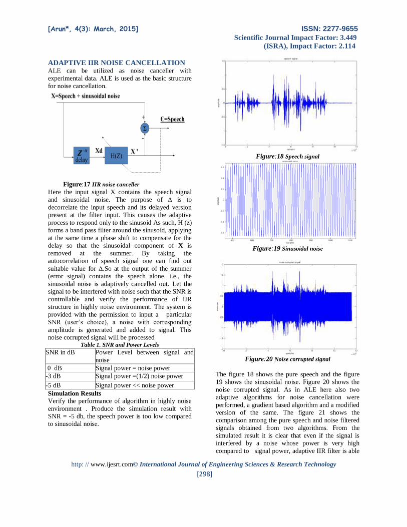
Simulation Results Verify the performance of algorithm in highly noise

environment . Produce the simulation result with

SNR = -5 db, the speech power is too low compared

to sinusoidal noise.

Figure:18 Speech signal

Figure:19 Sinusoidal noise

Figure:20 Noise corrupted signal

The figure 18 shows the pure speech and the figure

19 shows the sinusoidal noise. Figure 20 shows the

noise corrupted signal. As in ALE here also two

adaptive algorithms for noise cancellation were

performed, a gradient based algorithm and a modified

version of the same. The figure 21 shows the

comparison among the pure speech and noise filtered

signals obtained from two algorithms. From the

simulated result it is clear that even if the signal is

interfered by a noise whose power is very high

compared to signal power, adaptive IIR filter is able


[Arun*, 4(3): March, 2015] ISSN: 2277-9655




[299]

to pick out the noise. The blue colored signal is

obtained from normal algorithm. The red colored

signal is produced by modified algorithm. From the

figure below it is clear that the modified algorithm is

converging faster than the normal one. Hence

modified version of the gradient based algorithmis

used for implementation on PowerPC.

Figure:21 Input speech and noise filtered signals

IMPLEMENTATION Interference cancellation using adaptive IIR

algorithm is implemented in PowerPC 7448

SBC(Single Board Computer).

Figure:22 PowerPC 7448 SBC block diagram

Implementation process flow

The noise corrupted signal (Speech signal in the

presence of machinery noise)is captured by PC and

the data would be transferred to PowerPC through

network as packets. The PowerPC receives the data

and perform the adaptive algorithm, and the result is

send back to PC, the PC receives the processed data

(noise filtered signal), then gather the result from PC

C

C


[Arun*, 4(3): March, 2015] ISSN: 2277-9655




[300]

Figure:23 Implementation flow chart

RESULTS AND DISCUSSION The interference cancellation using IIR filter has been

implemented successfully on PowerPC 7448 with

Modified Gradient Based Adaptive algorithm and

verified the output. Here the signal applied to the

input is speech corrupted by machinery noise. After

adaptive filtering process speech alone is produced at

the output. Since the sound card for the new PowerPC 7448

has not yet developed and integrated to the board, for

the real time implementation sound cannot be directly

captured in PowerPC .So the following procedure is

used. The noise corrupted signal is captured by PC

and the data would be transferred to PowerPC

through network as packets. The PowerPC receives

the data and perform the algorithm, and the result is

again send to PC, the PC receives the processed data

(noise filtered signal), then playback the result from

PC. Figure 24 and Figure 25 shows the implemented

result.

Figure:24 Noise corrupted Speech signal

Figure:25 Noise corrupted and Noise filtered Speech

signals Figure 25 shows the noise corrupted signal and

noise filtered signal together. The Adaptive filter

filtered the machinery noise and produced the

speech alone at the output.

CONCLUSION A detailed survey on ANC is carried out and

observed that many fewer coefficients may be needed

to achieve the desired performance for IIR filter

when compared to FIR.From simulation under


[Arun*, 4(3): March, 2015] ISSN: 2277-9655




[301]

different noise environment, it is concluded that the

modified gradient based algorithm is more suitable

for Adaptive IIR noise cancellation. Even if the

signal is interfered by a noise whose power is very

high compared to signal power, adaptive IIR filter is

able to pick out the noise. i.e., even in the highly

noise environment adaptive IIR filter is powerful.

FUTURE SCOPE Future work includes the implementation of the

pipelined version of the filter for improved speed,

and to optimize the programmable processing

element at circuit level for efficient ASIC

implementation of the reconfigurable fabric.

ACKNOWLEDGEMENTS The authors would like to thankNPOL kochi[DRDO],

Government of India and National Institute of

Electronics and IT(NIELIT),Calicut for their help

with this work

REFERENCES 1. B. Widrow et al., “Adaptive noise

cancelling: Principles and applications,”

Proc. IEEE, vol. 63, pp. 1692-1716, Dec.

1975.

2. Don R. Hush et al., ”An Adaptive IIR

Structure for sinusoidal Enhancement,

Frequency Estimation and Detection”, IEEE

Trans. Acoust., Speech, Signal Processing,

vol.ASSP-34, No.6, pp.1380-1390,

Dec.1986.

3. Bijan Sayyarrodsari et al.,“An Estimation-

Based Approach to the design of Adaptive

IIR Filters”, Proceedings of the American

Control Conference Philadelphia,

Pennsylvania l June 1998.

4. J.J. Shynk. Adaptive IIR filtering. IEEE

ASSP Magazine, Vol. 6, No. 2, pp. 4-21,

April 1989.

5. M. Harteneck, R.W Stewart, “Adaptive

Digital Signal Processing Java Teaching

Tool” Submitted to IEEE Transactions on

Education - Special CDROM Issue,

November 1999.

6. S. Haykin: Adaptive Filter Theory,

Englewood Cliffs, N.J.: Prentice-Hall, Inc.,

4th

Edition (2001).

7. B. Widrow and S. Stearns: Adaptive Signal

Processing. Prentice Hall, 1985.

8. Farhang-Boroujeny,B. Adaptive filters:

theory and applications, John Wiley& sons

Ltd,1998.

9. Freescale semiconductor, “MPC 7448 RISC

Microprocessor Hardware Specifications” a

60 page PDF manual, 2005.

10. O.L Frost III ,”An algorithm for linearly

constrained adaptive array processing,”

Proc.IEEE,vol.60.pp.926-935 Aug 1972

11. Adaptive Filter Theory by Simen Haykin:

3rd edition,Pearson Education Asia.LPE

AUTHOR BIBLOGRAPHY

Arun.C

Assistant Professor, Dept of

ECE,College of Engineering

Perumon,Kollam,Kerala

Veena V S

Assistant Professor, Dept of

EEE,College of Engineering

Perumon,Kollam,Kerala


IMPLEMENTATION OF INTERFERENCE CANCELLATION BY ADAPTIVE FILTERS

Documents

Transcript of IMPLEMENTATION OF INTERFERENCE CANCELLATION BY ADAPTIVE FILTERS