arX

iv:h

ep-t

h/98

0707

6v3

21

Dec

199

8

hep-th/9807076LBNL-41932, SLAC-PUB-7875, SU-ITP-98/35, UCB-PTH-98/33

Vacuum Energy Cancellation ina Non-Supersymmetric String

Shamit Kachru1, Jason Kumar2 and Eva Silverstein3

1Department of Physics

University of California at Berkeley

Berkeley, CA 94720

and

Ernest Orlando Lawrence Berkeley National Laboratory

Mail Stop 50A-5101, Berkeley, CA 94720

2 Department of Physics

Stanford University

Stanford, CA 94305

3 Stanford Linear Accelerator Center

Stanford University

Stanford, CA 94309

We present a nonsupersymmetric orbifold of type II string theory and show that it has

vanishing cosmological constant at the one and two loop level. We argue heuristically that

the cancellation may persist at higher loops.

July 1998

1. Introduction

One of the most intriguing and puzzling pieces of data is the (near-)vanishing of the

cosmological constant Λ [1]. Unbroken supersymmetry would ensure that perturbative

quantum corrections to the vacuum energy vanish (in the absence of a U(1) D-term) due

to cancellations between bosonic and fermionic degrees of freedom. However, although

both bosons and fermions appear in the low-energy spectrum, they are not related by

supersymmetry and this mechanism for cancelling Λ is not realized.

Because string theory (M-theory) is a consistent quantum theory which incorporates

gravity, it is interesting (and necessary) to see how string theory copes with the cosmo-

logical constant. In a perturbative string framework, because the string coupling gst (the

dilaton) is dynamical, the quantum vacuum energy constitutes a potential for it. So the

issue of turning on a nontrivial string coupling is related to the form of the vacuum energy

in string theory.

In this paper we present a class of perturbative string models in which supersymmetry

is broken at the string scale but perturbative quantum corrections to the cosmological

constant cancel. We begin with a simple mechanism that ensures the (trivial) vanishing

of the 1-loop vacuum energy (as well as certain tadpoles and mass renormalizations).

We then compute the (spin-structure-dependent part of the) 2-loop partition function

and demonstrate that it vanishes. This requires some analysis of worldsheet gauge-fixing

conditions, modular transformations, and contributions from the boundaries of moduli

space. Examination of the general form of higher-loop amplitudes suggests that they

similarly may cancel and we next present this argument. We are unable to rigorously

generalize our 2-loop calculation to higher loops at this point because of the complications

of higher-genus moduli space. We hope to be able to make the higher-genus result more

precise by using an operator formalism as will become clearer in the text, though we leave

that for future work.

In addition we discuss how this model may fit into the framework [2] relating conformal

fixed lines/points in quantum field theory to vanishing dilaton potentials/isolated minima

of the dilaton potential in string theory. This provides hints as to where to look for more

general models with vanishing Λ. In particular we will be interested in models without the

tree level bose-fermi degeneracy that we have here, as well as models in which the dilaton is

stabilized. We should note in this regard that instead of working in 4d perturbative string

theory as we do here, we could consider the same class of models in 3d string theory and

1

consider the limit of large gst. If the appropriate D-brane bound states exist in this theory

to provide Kaluza-Klein modes of an M-theoretic fourth dimension, one could obtain in

this way 4d M-theory vacua with vanishing cosmological constant and no dilaton (in this

way similar to the scenario of [3], but here without the need for 3d supersymmetry).

We understand that a complementary set of models has been found in the free

fermionic description [4]. We would like to thank Zurab Kakushadze for pointing out

(and fixing) an error in our original model as presented at Strings ’98.

2. Nonabelian Orbifolds and the 1-loop Cosmological Constant

Consider the worldsheet path integral formulation of orbifold compactifications [5]. In

general one mods out by a discrete symmetry group of the 10-dimensional string theory.

This group involves rotations of the left and right-moving worldsheet scalars XµL,R and

fermions ψµL,R as well as shifts of the scalars Xµ

L,R. Here µ = 1, . . . , 10 is a spacetime

SO(9, 1) vector index. The worldsheet path integral at a given loop order h splits up into

a sum over different twist structures, in which the fields are twisted by orbifold group

elements in going around the various cycles of the genus-h Riemann surface Σh. These

twists must respect the homology relation

h∏

i=1

aibia−1i b−1

i = 1 (2.1)

where ai and bi are the canonical 1-cycles on Σh. In particular, at genus 1, one sums over

pairs (g, h) of commuting orbifold space group elements g and h.

g

h

Figure 1: Torus twisted by elements (g, h)

In considering nonsupersymmetric orbifolds, this suggests an interesting class of mod-

els. Consider orbifolds in which no commuting pair of group elements breaks all the

2

supersymmetry (i.e. projects out all of the gravitinos), but in which the full group does

break all the supersymmetry. At the one-loop level, each contribution to the path integral

then effectively preserves some supersymmetry and therefore vanishes. This is a formal

way of encoding the fact that the spectrum for this type of model will have bose-fermi

degeneracy at all mass levels (though no supersymmetry). So the one-loop partition func-

tion, as well as appropriate tadpoles, mass renormalizations, and three-point functions,

are uncorrected.

We will discuss the following specific model.1 Let us start with type II string theory

compactified on a square torus T 6 ∼ (S1)6 at the self-dual radius R = ls (where ls =√α′

is the string length scale). Consider the asymmetric orbifold generated by the elements f

and g:

S1 f g

1 (−1, s) (s,−1)

2 (−1, s) (s,−1)

3 (−1, s) (s,−1)

4 (−1, s) (s,−1)

5 (s2, 0) (s, s)

6 (s, s) (0, s2)

(−1)FR (−1)FL

We have indicated here how each element acts on the left and right moving RNS degrees

of freedom of the superstring. Here s refers to a shift by R/2. So for example f reflects the

left-moving fields X1...4L , ψ1...4

L and shifts X1...4R by R/2, X5

L by R, andX6 = 12(X6

L+X6R) by

R/2. In addition it includes an action of (−1)FR which acts with a (−1) on all spacetime

spinors coming from right-moving worldsheet degrees of freedom. This can be thought

of as discrete torsion [8]: in the right-moving Ramond sector the f -projection has the

opposite sign from what it would have without the (−1)FR action. Similarly the above table

indicates the action of the generator g on the worldsheet fields. This orbifold satisfies level-

matching and the necessary conditions derived in [8,9] for higher-loop modular invariance

(we do not know if these conditions are sufficient).

There are several features to note about the spectrum of this model. First, it is not

supersymmetric. In particular, f projects out all the gravitinos with spacetime spinor

1 Other similar models can be constructed, some of which do not actually require the group

to be nonabelian to get 1-loop cancellation [6,4,7].

3

quantum numbers coming from the right-movers. Similarly g projects out the gravitinos

with left-moving spacetime spinor quantum numbers. Because of the shifts included in

our orbifold action, there are no massless states in twisted sectors, so in particular no

supersymmetry returns in twisted sectors. Second, the model is nonetheless bose-fermi

degenerate. In particular the massless spectrum has 32 bosonic and 32 fermionic physical

states.

In addition to the spectrum of perturbative string states there is a D-brane spectrum

in this theory which one can analyze along the lines of [10].This will be of interest in placing

this example in a more general context in the final section.

Our orbifold group elements satisfy the following algebraic relations:

fg = gfT−1L TR fT q

L = T−qL f gT q

R = T−qR g (2.2)

where TL denotes a shift by R on X1...4L and TR denotes a shift by R on X1...4

R . Clearly

also f commutes with TR and g commutes with TL.

The first relation in (2.2) tells us that f and g do not commute in the orbifold space

group. Therefore at the one loop level they never both appear as twists (f, g) in the

partition function (i.e. we cannot twist by f on the a-cycle and by g on the b-cycle). Fur-

thermore we can check that no commuting pair of elements break all the supersymmetry.

In order to break the supersymmetry we would need pairs of the form (fT aLT

bR, gT

cLT

dR) or

(fT aLT

bR, fgT

cLT

dR), for arbitrary integers a, b, c, d, a, b, c, d. (We could also have the latter

form with f interchanged with g but these are isomorphic.) By using the relations (2.2)

we see that neither pair of elements commutes:

(fT aLT

bR)(gT c

LTdR) = (gT c

LTdR)(fT a

LTbR)T 2c+1

L T 1−2bR (2.3)

So there is no choice of integers a, b, c, d for which the two elements commute in the space

group of the orbifold. Similarly

(fT aLT

bR)(fgT c

LTdR) = (fgT c

LTdR)(fT a

LTbR)T 2c−2a−1

L T 1−2bR (2.4)

So at the one loop level, there will not be any contribution to the partition function.

4

3. The 2-loop vacuum energy

At two loops the orbifold algebra itself does not automatically ensure the cancellation

of the partition function. Let us denote the canonical basis of 1-cycles by 2h-dimensional

vectors (a1, . . . , ah; b1, . . . , bh). At genus two, we run into twist structures like (1, 1; f, g)

around the canonical cycles:

f g

Figure 2: Basic twist structure at genus 2.

In the figure we indicate the cuts in the diagram in a given twist structure–here

the fields are twisted in going around the b-cycles, as in doing so they pass through the

indicated cuts. In particular this diagram involves both f and g twists, and therefore has

the information about the full supersymmetry breaking of the model. Is there reason to

believe the vacuum energy might nonetheless cancel? Heuristically, the following argument

suggests that we should indeed expect a cancellation. Consider evaluating the diagram

of Figure 2 near the factorization limit in which the diagram looks like a propagator

tube connecting two tori. Because of the homology relations, in this twist structure the

intermediate state in this propagator is untwisted. The diagram thus becomes a sum

over products of tadpoles of untwisted propagating states (weighted by e−mT where m

is the mass of the state and T gives the length of the tube). Each term is a tadpole of

the untwisted state in the g-twisted theory times a tadpole of the untwisted state in the

f -twisted theory. The contour deformation arguments of [11] imply that these tadpoles

vanish. In order to make this rigorous one needs to see explicitly that unphysical states

decouple properly (which only has to happen after summing over all twist structures). In

what follows we will provide an explicit computation of the 2-loop contribution and verify

that it vanishes.

3.1. Back to 1-loop.

In order to appreciate the relevant mechanism, it is worth returning momentarily to

the 1-loop (supersymmetric) contribution (1, f).

5

f

Figure 3: One-loop diagram with an f twist on the b cycle.

This contribution must vanish by supersymmetry, but it is instructive to observe how

the spin structure sum works in this case before going on to our 2-loop diagram. The

amplitude is

A1 =

∫

d2τ

(Imτ)2Tr(qL0 qL0f) (3.1)

where q = e2πiτ and L0 and L0 are the usual Virasoro zero mode generators. Let us consider

the spin-structure dependent piece of this amplitude. As explained in [12], the determinants

for the worldsheet Dirac operators acting on the RNS fermions are proportional to theta

functions. The θ-function is defined (for general genus h) by

θ[α, β](z|τ) =∑

n

e[πi(n+α)tτ(n+α)+2πi(n+α)(z+β)] (3.2)

Here z ∈ Ch/(ZZh + τZZh) and τ is the period matrix of the Riemann surface, defined in

terms of the canonical basis of holomorphic 1-forms ωi by∮

ajωi = δij and

∮

bjωi = τij.

The characteristics α, β encode the spin structure [13], i.e. the boundary conditions of the

fermions around the a and b cycles respectively of the Riemann surface. So for example if

α1 = 1/2 (resp. 0), the corresponding fermion has periodic (resp. antiperiodic) boundary

conditions around the a1 cycle.

The integrand of the 1-loop amplitude (3.1) is proportional to

A1 ∝∑

α,β

ηα,βθ2[α, β](0|τ)θ2[α, β +

1

2](0|τ) (3.3)

where ηα,β are the phases encoding the GSO projection. The first θ2 factor comes from

the left-moving RNS fermions ψ1...4L and the second θ2 factor comes from the other four

transverse left-moving fermions ψ5...8L . The symmetry between these two factors will play

6

an important role for us. Let us consider first the terms in the sum (3.3) with α = 1/2.

This describes left-moving Ramond-sector states propagating in the loop, as the left-moving

fermions ψL are periodic around the a-cycle. Because we have an f -twist around the b-

cycle, half the ψµL are periodic around the b-cycle and half are antiperiodic around the

b-cycle for each value of β in the sum. Thus in each α = 1/2 term half the RNS fermions

have zero modes, so these terms identically vanish.

Let us now consider the terms with α = 0, which describe left-moving Neveu-Schwarz

states propagating in the loop. These give

∑

β=0,1/2

η0,βθ2[0, β](0|τ)θ2[0, β + 1/2](0|τ). (3.4)

Note that both terms in this sum have the same functional form (θ2[0, 1/2](0|τ)θ2[0, 0](0|τ)).The only issue left is then the relative phase between them. The sum over β is simply the

GSO projection on the states propagating around the b-cycle. Let us normalize η0,0 to 1.

Then η0,1/2 = −1. This follows from the fact that in the NS sector the GSO projection

operator is 1−(−1)F . This encodes the fact that we must project onto odd fermion number

in the superstring in order to project out the tachyon which would otherwise come from

the vacuum at the −1/2 mass level. So our integrand is

(1 − 1)θ2[0, 0]θ2[0, 1/2] = 0. (3.5)

3.2. 2-loops with supersymmetry

In order to proceed to the 2-loop computation, we must consider various subtleties

arising in string loop computations for strings with worldsheet supersymmetry. (See for

example [14,15,16] for reviews with some references.) Let us begin by briefly reviewing

some of the issues in the supersymmetric case. We will work in the RNS formulation; for

discussion of the supersymmetric case in Green-Schwarz language see for example [17].

In performing the Polyakov path integral at genus h, we must integrate over all the

worldsheet fields including the worldsheet metric h and gravitino χ. This infinite dimen-

sional space is reduced to a finite dimensional space of (super-)moduli by dividing out

the diffeomorphisms and local supersymmetry transformations. There are 3h− 3 complex

bosonic moduli τ and 2h − 2 complex supermoduli ζ. At genus h = 2 we can take the

gravitino to have delta-function support on the worldsheet for even spin structures [18].

(For odd spin structures the amplitude vanishes as a result of the integration of fermionic

zero modes.)

7

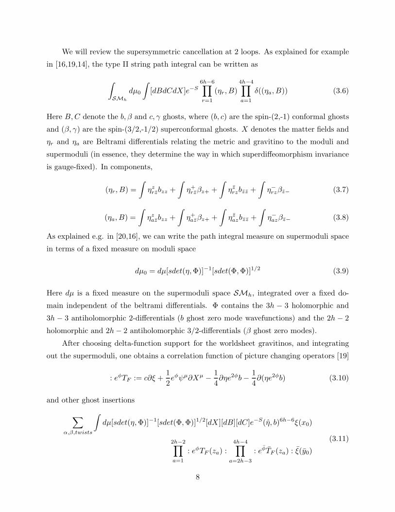
We will review the supersymmetric cancellation at 2 loops. As explained for example

in [16,19,14], the type II string path integral can be written as

∫

SMh

dµ0

∫

[dBdCdX ]e−S6h−6∏

r=1

(ηr, B)4h−4∏

a=1

δ((ηa, B)) (3.6)

Here B,C denote the b, β and c, γ ghosts, where (b, c) are the spin-(2,-1) conformal ghosts

and (β, γ) are the spin-(3/2,-1/2) superconformal ghosts. X denotes the matter fields and

ηr and ηa are Beltrami differentials relating the metric and gravitino to the moduli and

supermoduli (in essence, they determine the way in which superdiffeomorphism invariance

is gauge-fixed). In components,

(ηr, B) =

∫

ηzrzbzz +

∫

η+rzβz+ +

∫

ηzrzbzz +

∫

η−rzβz− (3.7)

(ηa, B) =

∫

ηzazbzz +

∫

η+azβz+ +

∫

ηzazbzz +

∫

η−azβz− (3.8)

As explained e.g. in [20,16], we can write the path integral measure on supermoduli space

in terms of a fixed measure on moduli space

dµ0 = dµ[sdet(η,Φ)]−1[sdet(Φ,Φ)]1/2 (3.9)

Here dµ is a fixed measure on the supermoduli space SMh, integrated over a fixed do-

main independent of the beltrami differentials. Φ contains the 3h − 3 holomorphic and

3h − 3 antiholomorphic 2-differentials (b ghost zero mode wavefunctions) and the 2h − 2

holomorphic and 2h− 2 antiholomorphic 3/2-differentials (β ghost zero modes).

After choosing delta-function support for the worldsheet gravitinos, and integrating

out the supermoduli, one obtains a correlation function of picture changing operators [19]

: eφTF := c∂ξ +1

2eφψµ∂Xµ − 1

4∂ηe2φb− 1

4∂(ηe2φb) (3.10)

and other ghost insertions

∑

α,β,twists

∫

dµ[sdet(η,Φ)]−1[sdet(Φ,Φ)]1/2[dX ][dB][dC]e−S(η, b)6h−6ξ(x0)

2h−2∏

a=1

: eφTF (za) :

4h−4∏

a=2h−3

: eφTF (za) : ξ(y0)

(3.11)

8

The superconformal ghosts β = ∂ξe−φ, γ = ηeφ are defined in terms of spin-0 and spin

-1 fermions ξ, η and a scalar φ [11]. The spin-0 fermion ξ has a zero mode on the surface

which is absorbed by the insertion of ξ(x0) in (3.11). There is an anomaly in the ghost

number U(1) current which requires insertions of operators with total ghost number 2h−2

to get a nonvanishing result. The correlation functions (3.11) can be evaluated using the

formulas derived in e.g. [21,22].

We will now fix the gauge for the gravitinos by making a definite choice of points z1,2.

As explained in [14], the choice of points must be taken in such a way that the gauge slice

chosen is transverse to the gauge transformations. It must also respect modular invariance

of the amplitude [19,14]. Ultimately, we will be interested in a gauge choice for which

z1, z2 → ∆γ , where ∆γ is a divisor corresponding to an odd spin structure γ, that is a

point where a holomorphic 1/2-differential has a zero. As explained in [14], this choice

(which amounts to putting the insertions at one of the branch points in a hyperelliptic

description of the surface) satisfies transversality. It was argued in [23,24] that despite

earlier worries [14], this choice is also consistent with modular invariance. The modular

invariance is not manifest in the description in terms of θ-functions, as the calculation of

correlation functions on the Riemann surface [21] involve a choice of reference spin structure

δ. Having to choose a spin structure naively appears to violate modular invariance. Had

we chosen a different reference spin structure δ′, we would have shifted the arguments of

our theta functions by elements n+mτ of the Jacobian lattice. Such a shift introduces a

τ -dependent phase multiplying the θ-function–the θ-functions transform as sections of line

bundles over the Jacobian torus. These phases must cancel out of the properly defined

integrand, and in [23] this was demonstrated explicitly for certain (nonvanishing) 2-loop

contributions.

We need to consider the (left-moving) spin-structure-dependent pieces of the correla-

tion function, the poles arising from the spin-structure-independent local behavior of the

picture changing correlator, and the behavior of the determinant (3.9) in this gauge. Ac-

cording to [19] we have the following contributions to the spin-structure-dependent pieces

of the 2-loop partition function. The matter part of TF contributes

∑

δ

〈δ|γ〉θ[δ]4(0)θ[δ](z1 − z2)

θ[δ](z1 + z2 − 2∆γ)(3.12)

Here δ ≡ (α, β) encodes the spin structure of the various contributions and 〈δ|γ〉 =

e4πi(αγ2−βγ1) encodes the GSO phases [25]. Here the arguments∑

p − ∑

q in terms of p

9

and q which are sets of points on the Rieman surface is shorthand for the Jacobi vector∑

∫ p

p0

ωi −∑

∫ q

p0

ωi.

Let us first, following [23], take z1 + z2 = 2∆γ , that is place z1 + z2 at a divisor

corresponding to the canonical class, without setting z1 = z2. The contribution (3.12)

then simplifies to

∑

δ

〈δ|γ〉θ[δ]3(0)θ[δ](z1 − z2) = 4θ[γ]4(z1 − ∆γ) (3.13)

where in the last step we have used a Riemann identity. The Riemann Vanishing Theorem

then implies that this vanishes identically as a function of z1 [23]. Thus in this case

whatever poles arise as z1 → z2, the identical zero from the spin structure sum cancels it.

Now turning to the ghost piece of the correlation function of picture-changing opera-

tors, one obtains contributions isomorphic to (3.13) as well as

ωi(z1)θ[δ]5(0)∂iθ[δ](2z2 − 2∆γ)

θ2[δ](z1 + z2 − 2∆γ)(3.14)

Here ωi are the canonical basis of holomorphic one-forms on the Riemann surface, satisfying∫

aiωj = δij and

∫

biωj = τij where τ is the period matrix for the surface. Again simplifying

this by first taking z1 + z2 = 2∆γ we obtain

∑

δ

〈δ|γ〉∂z1(θ[δ]3(0)θ[δ](z1 − z2)) = 4∂z1

(θ[γ]4(z1 − ∆γ)) (3.15)

Because the right-hand side of this expression is a derivative of 0 (by the Riemann vanishing

theorem), it vanishes identically. Again any poles from the picture changing OPEs are

irrelevant [23].

3.3. (Non-)Superstring Perturbation Theory

In an orbifold model, one can consider separately different twist structures, and ana-

lyze the fundamental domain of the modular group that preserves a given twist structure.

In general there are an infinite number of contributions coming from different choices of

bosonic shifts. In §4 we will analyze the twist structure of Figure 2 (with no additional

bosonic shifts) and see that the resulting modular group acts freely on τ . In this situation,

the choice of a branch point for z1,2 is manifestly modular invariant; the possible obstruc-

tion to modular invariance discussed in [19,14] does not arise, as there are no orbifold

points in the moduli space. We also analyze in §4 the boundary contributions and see that

10

they vanish. One can show that with arbitrary additional shifts (respecting the homology

relation of the Riemann surface) there are still no orbifold points in the moduli space.

We will analyze the twist structure (1, 1, f, g) (it will later be shown why this is the

only twist structure which needs to be analyzed). The f twist affects the characteristics

of some of the θ functions (arising from twisted fields) by shifting them by (0, 0, 1/2, 0) –

we shall denote this as a shift by 12L. κ will be defined as γ + (0, 0, 0, 1/2), and we choose

γ such that both γ and κ are odd.

The correlation function of the matter part of the picture changing operators breaks

into two contributions. The terms involving 〈ψi∂X i(z1)ψi∂X i(z2)〉 with i = 5, · · ·10 give

∑

δ

〈κ|δ〉θ[δ](0)2θ[δ + 12L](0)2θ[δ](z1 − z2)

θ[δ](z1 + z2 − 2∆γ)

×(pµi ω

i(z1)pµj ω

j(z2)1

E(z1, z2)2+

6

E(z1, z2)2∂z1

∂z2logE(z1, z2))

×det(Φ3/2a (zb))

(3.16)

Upon setting z1 + z2 = 2∆γ we can cancel the denominator against one factor in the

numerator to get

∑

δ

〈κ|δ〉θ[δ](0)θ[δ](z1 − z2)θ[δ+1

2L](0)2 = 4θ[κ](

1

2(z1 − z2))θ[κ+

1

2L](

1

2(z1 − z2)) (3.17)

for the spin-dependent piece of this correlator. Because κ is an odd spin structure, this

vanishes like (z1 − z2)2. As z1 → z2 the determinant factor (3.9) produces another zero:

plugging in the delta function ηa we obtain

[sdet(η,Φ)]−1 ∝ det(ηa,Φ3/2b ) = det(Φ

3/2b (za)) (3.18)

Here Φ3/2b , b = 1, 2 form a basis of holomorphic 3/2-differentials. As the za approach each

other, the determinant (3.18) goes to zero, so all in all (3.16) has a (z1 − z2)3 multiplying

the prime forms. However, since the prime-forms are yielding poles as z1 → z2, it remains

to check that there are no finite pieces in (3.16).

Note that E(z1, z2) goes like z1 − z2 as z1 → z2. Thus, the terms proportional to1

E(z1,z2)2times the loop momenta clearly vanish in the limit, since there is only a second

order pole from the prime forms which cannot cancel the third order zero we found from

the spin structure sum and the superdeterminant. This leaves the term which goes like

11

1E(z1,z2)2

∂z1∂z2

logE(z1, z2). Using the fact that E(z1, z2) has a Taylor expansion of the

form

E(z1, z2) ∼∞∑

n=0

cn(z1 − z2)2n+1 (3.19)

as z1 → z2, one sees that this combination of prime forms has an expansion

1

E(z1, z2)2∂z1

∂z2logE(z1, z2) ∼

∞∑

n=−2

dn(z1 − z2)2n (3.20)

On the other hand, the determinant factor is an odd function of z1 − z2 with an expansion

of the form

det(Φ3/2a (zb)) ∼

∞∑

m=0

em(z1 − z2)2m+1 (3.21)

while the sum over spin structures (3.17) is an even function with a second order zero at

z1 = z2. From these facts, it is easy to see that the full expression (3.16) has an expansion

of the form∞∑

j=0

fj(z1 − z2)2j−1 (3.22)

as z1 → z2.

Examining (3.22), we see that

• There are no finite contributions as z1 → z2.

• There is a (gauge artifact) pole as z1 → z2; in fact this pole receives contributions from the

various matter and ghost correlators proportional to the matter/ghost central charges, and

hence cancels once all of the terms are taken into account (since ctot = cmatter+cghost = 0).

We will see this explicitly once we compute the remaining matter and ghost contributions.

The second type of matter correlator arises from contracting the ψi∂X i(z1)ψi∂X i(z2)

with i = 1, · · ·4. This leads to a contribution

∑

δ

〈κ|δ〉θ[δ](0)3θ[δ + 12L](0)θ[δ + 1

2L](z1 − z2)

θ[δ](z1 + z2 − 2∆γ)

×(pµi ω

i(z1)pµj ω

j(z2)1

E(z1, z2)2+

4

E(z1, z2)2∂z1

∂z2logE(z1, z2))

×det(Φ3/2a (zb))

(3.23)

Choosing z1 + z2 = 2∆γ , the spin sum in (3.23) simplifies to

∑

δ

〈κ|δ〉θ[δ](0)2θ[δ +1

2L](0)θ[δ +

1

2L](z1 − z2) (3.24)

12

which, after applying a Riemann identity, becomes

4θ[κ](1

2(z1 − z2))

2θ[κ+1

2L](

1

2(z1 − z2))

2 (3.25)

So in fact after summing over spin structures this looks the same as the spin sum of the

first type of matter contribution (3.17). Again, it vanishes like (z1 − z2)2 as z1 → z2.

Now, the argument for the cancellation proceeds as it did for the first type of matter

contribution. The terms involving only the 1E(z1,z2)2

multiplying loop momenta only have a

second order pole, which cannot cancel the third order zero coming from the determinant

times the spin structure sum (3.25). The terms involving higher inverse powers of the

prime forms lead to a simple pole (which cancels after summing over matter and ghosts,

as it is proportional to the total central charge) and no finite contributions.

Next, let us consider the terms in the correlator of picture changing operators coming

from the ghost part of the worldsheet supercurrent These terms take the form

〈−1

4c∂ξ(z1)

(

2∂ηe2φb+ η∂e2φb+ ηe2φ∂b)

(z2)〉

+〈−1

4

(

2∂ηe2φb+ η∂e2φb+ ηe2φ∂b)

(z1)c∂ξ(z2)〉 .(3.26)

There are three types of terms that arise [19]. We are in the twist structure (1, 1, f, g).

As in the matter sector, the f twist affects the characteristics of the θ-functions arising

in the worldsheet correlation functions and determinants. We will denote the shift in the

characteristic, which is (0, 0, 1/2, 0), as 12L. The first type of contribution is

∑

δ

〈κ|δ〉θ[δ](0)3θ[δ + 12L](0)2θ[δ](2z2 − 2∆γ)θ(z1 − z2 +

∑

w − 3∆)

θ[δ](z1 + z2 − 2∆γ)2E(z1, z2)3

×det(Φa(zb))

∏

E(z1, w)∏

E(z2, w)∂z1

log(

∏

E(z1, w)

E(z1, z2)5σ(z1))

+(z1 ↔ z2)

(3.27)

The second is

∑

δ

〈κ|δ〉θ[δ](0)3θ[δ + 12L](0)2ωi(z1)∂

iθ[δ](2z2 − 2∆γ)θ(z1 − z2 +∑

w − 3∆)

θ[δ](z1 + z2 − 2∆γ)2E(z1, z2)3

×det(Φa(zb))

∏

E(z1, w)∏

E(z2, w)

+(z1 ↔ z2)

(3.28)

13

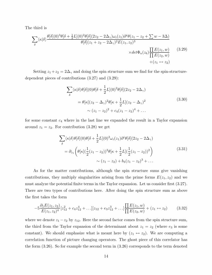
The third is

∑

δ

〈κ|δ〉θ[δ](0)3θ[δ + 12L](0)2θ[δ](2z2 − 2∆γ)ωi(z1)∂

iθ(z1 − z2 +∑

w − 3∆)

θ[δ](z1 + z2 − 2∆γ)2E(z1, z2)3

×detΦa(zb)

∏

E(z1, w)∏

E(z2, w)

+(z1 ↔ z2)

(3.29)

Setting z1 +z2 = 2∆γ and doing the spin structure sum we find for the spin-structure-

dependent pieces of contributions (3.27) and (3.29):

∑

δ

〈κ|δ〉θ[δ](0)θ[δ+1

2L](0)2θ[δ](2z2 − 2∆γ)

= θ[κ](z2 − ∆γ)2θ[κ+1

2L](z2 − ∆γ)2

∼ (z1 − z2)2 + c4(z1 − z2)

4 + . . .

(3.30)

for some constant c4 where in the last line we expanded the result in a Taylor expansion

around z1 = z2. For contribution (3.28) we get

∑

δ

〈κ|δ〉θ[δ](0)θ[δ +1

2L](0)2ωi(z1)∂

iθ[δ](2z2 − 2∆γ)

= ∂z1

(

θ[κ](1

2(z1 − z2))

2θ[κ+1

2L](

1

2(z1 − z2))

2

)

∼ (z1 − z2) + b3(z1 − z2)3 + . . .

(3.31)

As for the matter contributions, although the spin structure sums give vanishing

contributions, they multiply singularities arising from the prime forms E(z1, z2) and we

must analyze the potential finite terms in the Taylor expansion. Let us consider first (3.27).

There are two types of contributions here. After doing the spin structure sum as above

the first takes the form

−5∂1E(z1, z2)

E(z1, z2)4[z2

12 + c4z412 + . . .][z12 + e3z

312 + . . .]

∏

E(z1, w)∏

E(z2, w)+ (z1 ↔ z2) (3.32)

where we denote z1−z2 by z12. Here the second factor comes from the spin structure sum,

the third from the Taylor expansion of the determinant about z1 = z2 (where e3 is some

constant). We should emphasize what is meant here by (z1 ↔ z2). We are computing a

correlation function of picture changing operators. The ghost piece of this correlator has

the form (3.26). So for example the second term in (3.26) corresponds to the term denoted

14

z1 ↔ z2 in (3.32). So in particular the second term involves interchanging the operators

in the ghost correlator, without changing z1 to z2 in the determinant factor. The first

and fourth factors involving the prime forms encode the physical poles and zeroes of the

correlator. The leading singularity from the prime forms here comes from the 1/z412 term

in the expansion of the prime form factors. Therefore only the leading term in the Taylor

expansion of the spin structure sum and determinant factors potentially survive (so we

can ignore the terms proportional to c4 or e3, which give fifth-order zeroes). Similarly

expanding the prime forms E(z1, z2) gives a subleading term with only a 1/z212 pole, which

is cancelled by the third order zero coming from the leading piece of the spin structure

sum times determinant.

Putting the factors together, we see that the leading piece is a simple pole in z12. The

first three factors in (3.32) are the same in the term with z1 ↔ z2. When we include the

term with z1 ↔ z2, they multiply the prime form factor

∏

E(z1,w)∏

E(z2,w)+

∏

E(z2,w)∏

E(z1,w). This is even

under z1 ↔ z2. In our Taylor expansion it therefore becomes of the form O(1)+f2z212+ . . .,

and only the first term contributes. Therefore in Taylor expanding the contribution (3.32),

we get a pole piece plus higher order terms which vanish in the limit z1 → z2. In particular,

no finite pieces survive. What is the interpretation of the pole piece? It is proportional

to the ghost central charge, and precisely cancels the pole piece coming from the matter

contribution.

The second type of contribution in (3.27) takes the form

1

E(z1, z2)3[z2

12 + . . .][z12 + . . .]

∏

E(z1, w)∏

E(z2, w)∂1log(

∏

E(z1, w)

σ(z1)) (3.33)

where the . . . denotes terms which vanish automatically as z1 → z2. The leading pole from

the prime forms here is cubic. Before including the z1 ↔ z2 term there is a finite piece

obtained by multiplying this times the third order zero obtained from the spin structure

sum and determinant factors. The spin structure sum is even under the interchange of

z1 and z2 in this case, and as discussed above the determinant factor is the same in both

terms. The factor 1E(z1,z2)3

does change sign between the two terms, however. So when we

add the (z1 ↔ z2) term the contribution cancels.

Let us now consider the contribution (3.28). This gives a contribution of the form

1

E(z1, z2)3[z12 + . . .][z12 + . . .]

(∏

E(z1, w)∏

E(z2, w)+

∏

E(z2, w)∏

E(z1, w)

)

(3.34)

15

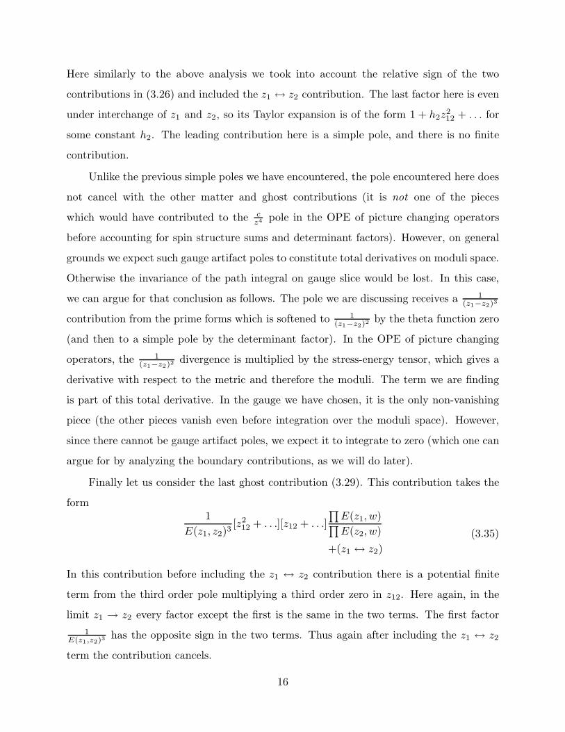
Here similarly to the above analysis we took into account the relative sign of the two

contributions in (3.26) and included the z1 ↔ z2 contribution. The last factor here is even

under interchange of z1 and z2, so its Taylor expansion is of the form 1 + h2z212 + . . . for

some constant h2. The leading contribution here is a simple pole, and there is no finite

contribution.

Unlike the previous simple poles we have encountered, the pole encountered here does

not cancel with the other matter and ghost contributions (it is not one of the pieces

which would have contributed to the cz4 pole in the OPE of picture changing operators

before accounting for spin structure sums and determinant factors). However, on general

grounds we expect such gauge artifact poles to constitute total derivatives on moduli space.

Otherwise the invariance of the path integral on gauge slice would be lost. In this case,

we can argue for that conclusion as follows. The pole we are discussing receives a 1(z1−z2)3

contribution from the prime forms which is softened to 1(z1−z2)2

by the theta function zero

(and then to a simple pole by the determinant factor). In the OPE of picture changing

operators, the 1(z1−z2)2 divergence is multiplied by the stress-energy tensor, which gives a

derivative with respect to the metric and therefore the moduli. The term we are finding

is part of this total derivative. In the gauge we have chosen, it is the only non-vanishing

piece (the other pieces vanish even before integration over the moduli space). However,

since there cannot be gauge artifact poles, we expect it to integrate to zero (which one can

argue for by analyzing the boundary contributions, as we will do later).

Finally let us consider the last ghost contribution (3.29). This contribution takes the

form1

E(z1, z2)3[z2

12 + . . .][z12 + . . .]

∏

E(z1, w)∏

E(z2, w)

+(z1 ↔ z2)

(3.35)

In this contribution before including the z1 ↔ z2 contribution there is a potential finite

term from the third order pole multiplying a third order zero in z12. Here again, in the

limit z1 → z2 every factor except the first is the same in the two terms. The first factor

1E(z1,z2)3

has the opposite sign in the two terms. Thus again after including the z1 ↔ z2

term the contribution cancels.

16

4. Boundary Contributions

In the previous section, we studied the two loop diagram with twists by f and g going

around the b1,2 cycles, i.e. with twist structure (1, 1, f, g). We saw that the computation

yields a vanishing integrand if we make a very specific choice of insertion points for the

picture-changing operators : eφTF :. Since the answer should be independent of the choice

of these insertion points, this seems to imply that the two loop vacuum energy vanishes.

However, under a change of the choice of insertion points, it can be shown that the

computation changes by a total derivative [19,26]

∫

F

∂ω (4.1)

where F is the appropriate fundamental domain of integration for the computation. There-

fore, one must worry about contributions arising at the boundary of F [14].

4.1. The Fundamental Domain

What is the fundamental domain F for this computation? At genus two, the Te-

ichmuller space is given very explicitly in terms of the Siegel upper half space of 2 × 2

matrices:

H2 = {τ2×2 : τ tr = τ, Im τ > 0}

τ is the period matrix of the genus two surface. The modular group at genus two is

G = Sp(4,ZZ). The moduli space can then be constructed by taking the quotient of H2 by

G. One must also remove the modular orbit of the diagonal matrices.

For our computation, on the other hand, we have twists (1, 1, f, g) about the

(a1, a2, b1, b2) cycles of the surface. Therefore, we need to integrate the correlator of the

picture changing operators over F = H2/G, where G is the subgroup of Sp(4,ZZ) which

preserves the twist structure (1, 1, f, g).

It is easy to see that the allowed matrices are the ones that act on the homology

(a1, a2, b1, b2) like

a b 0 0c d 0 0x y 1 0z w 0 1

(4.2)

17

Denoting the 2 × 2 blocks as

(

A BC D

)

we must impose

AtrC = CtrA, BtrD = DtrB, AtrD − CtrB = 1 (4.3)

which is just the requirement that (4.2) is in Sp(4,ZZ). This further restricts the allowed

matrices (4.2) to be of the form

1 0 0 00 1 0 0x y 1 0y w 0 1

(4.4)

Now, if

(

A BC D

)

acts on the homology, then the action on the period matrix τ is

given by

(

D CB A

)

– in other words,

τ → (Dτ + C) (Bτ + A)−1 (4.5)

So from the allowed actions on the homology (4.4), we see that the identifications to be

made on the period matrices are

(

τ1 τ12τ12 τ2

)

→(

τ1 + x τ12 + yτ12 + y τ2 + w

)

(4.6)

In addition, positivity of Im τ requires that

Im τ1,2 > 0, (Im τ12)2 < Im τ1 Im τ2 (4.7)

The constraints (4.6) and (4.7) together yield the correct fundamental domain F ⊂ H2

for our computation. τ1,2 live on strips with real part between (−1/2, 1/2) and positive

imaginary part, while τ12 has real part between (−1/2, 1/2) and imaginary part bounded

above and below by the second inequality in (4.7). Also, we must recall that in describing

the moduli space of Riemann surfaces in terms of H2, we had to delete the modular orbit

of diagonal matrices, yielding an additional boundary at τ12 → 0.

18

4.2. The Boundaries

Now that we have determined F , we can look for boundaries where the total deriva-

tive (4.1) might give a contribution after integration by parts. There are in fact three

boundaries in F . We will examine each of these boundaries in turn, and argue that no

boundary contribution exists.

1) τ1 or τ2 → i∞

g

f

Figure 4: Picture of boundary 1).

In this limit, one of the handles degenerates to a semi-circle glued on to the “fat” handle

at two points (i.e. a homology cycle collapses). It was argued in [14] that in such a limit,

no boundary contribution exists in theories without physical tachyons. Our theory has no

physical tachyons, so we will receive no contribution from this boundary.

2) τ12 → 0

fg

Figure 5: Picture of boundary 2).

In this limit, the genus two surface degenerates into two tori connected by a very long,

thin tube. Only massless physical states propagate in this tube [14], and in this limit the

genus two vacuum amplitude is related to a sum of products of one loop tadpoles for the

massless states.

The relevant one loop tadpoles are computed on tori with twists (1, f) or (1, g) around

the (a, b) cycles. Now, the f and g twist alone preserve d = 4, N = 2 supersymmetry. So,

19

there are no one loop tadpoles for states in the f or g twisted theory. This implies that

the genus two diagram vanishes in this limit.

3) Im τ1,2 → 0 or (Im τ12)2 → (Im τ1) (Im τ2)

To see the vanishing in this limit, we recall that the integrand for the vacuum amplitude

contains a factor of e−S(X), i.e. the action for map from the genus two surface to spacetime.

The relevant maps (given the f and g twists about the b cycles of the surface) wind around

the X5 and X6 directions of spacetime. This yields a contribution to the action which goes

like

S ≃ R2

α′{ Im τ1 + Im τ2Im τ1 Im τ2 − (Im τ12)2

} (4.8)

where R is the radius of the X5 and X6 circles [27,28]. Now, positivity of Im τ comes to

the rescue:

• If Im τ1 → 0 at fixed Im τ2, then the second inequality in (4.7) implies that S → ∞.

• If Im τ1,2 → 0, one can prove that the denominator in (4.8) vanishes as the square of

the numerator (once again using positivity of Im τ), so S → ∞.

• If Im τ1,2 are fixed and (Im τ12)2 approaches Im τ1 Im τ2, it is obvious that the action

diverges.

The upshot is that the e−S(X) in the integrand vanishes quickly enough at this boundary

to rule out any contributions.

4.3. Cases with Shifts

In additional to the amplitude (1, 1, f, g) which knows about the supersymmetry

breaking at genus two, there are other genus 2 amplitudes with (1, 1, f, g) twists on the

worldsheet fermions around the (a1, a2, b1, b2) cycles but with additional shifts acting on

the bosonic fields. In fact we show in §5 that this is (up to modular transformations) the

full set of supersymmetry breaking diagrams that we need to consider at genus two.

In each twist structure we will find that the spin-structure dependent part of the

vacuum amplitude vanishes. This leaves the issue of possible boundary contributions.

After summing over the various twist structures, we know the genus two vacuum energy

can be written as an integral over M2, the moduli space of genus two Riemann surfaces.

The possible boundary contributions (after we compactify M2) will come from boundaries

of type 1) and 2) in §4.2 (where a handle collapses or the surface degenerates into two

20

surfaces of lower genus connected by a long, thin tube). Hence, if we can argue that with

arbitrary twist and shift structures on the a, b cycles the vacuum amplitude vanishes at

boundaries of type 1) and 2), we will be done.

As we will discuss in §5, up to additional shifts on various cycles the possible structures

(which break all of the supersymmetry) are basically (1, 1, f, g), (f, g, g, f) and (f, fg, fg, f)

(up to possible exchanges of the role of f and g). Since we could use modular transfor-

mation to relate these to (1, 1, f, g) twist structure on the fermions, the spin-structure

dependent piece of the amplitude vanishes in each of these cases. In addition, each of

these vanishes at boundaries of type 1) because there are no physical tachyons. This

leaves the analysis of boundary 2).

Any amplitude with (1, 1, f, g) twists on the fermions, regardless of additional shifts,

vanishes at boundary 2) because it can be written as a product of tadpoles in the N = 2

supersymmetric f and g orbifolds (as in §4.2). On the other hand, the amplitude with

twist (f, g, g, f) would naively yield a product of one loop tadpoles in a nonsupersymmetric

theory. However, it turns out that the state propagating on the tube between the first and

second handle must be a massive state because it must be twisted to be emitted from

the “subtorus” with (f, g) twist on its (a, b) cycles. Since only massive states can run

in the tube, there is no contribution at the boundary of moduli space (where the tube

becomes infinitely long). A similar discussion applies to the (f, fg, fg, f) twist structure

with arbitrary shifts.

5. Twists at Genus h ≥ 2

A priori on a genus h Riemann surface, one needs to consider any combination of

twists on the various cycles ai, bi for i = 1, · · · , h consistent with the relation

a1b1a−11 b−1

1 · · ·ahbha−1h b−1

h = 1 (5.1)

In this section, we will argue that in fact using modular transformations one can greatly

reduce the kinds of twist structures that one needs to consider.

For our considerations, we do not need to worry about twists that preserve some of the

spacetime supersymmetry at genus h (for instance, twists only by f around various cycles).

The real concern will be sets of twists around different cycles which break the full spacetime

supersymmetry. We will now show that, up to inducing shifts on the worldsheet bosons

around some cycles, one only has to consider f and g twists on the bh−1 and bh cycles with

21

no twists on any other cycles. Any twist which breaks all of the spacetime supersymmetry

can be brought to this canonical (1, · · ·1, f, g) form by modular transformations.

Since in this section we will be ignoring the possible shifts on bosons around various

cycles (we’re only interested in the f, g action on fermions), we can use relations like

f2 = g2 = 1, fg = gf (5.2)

which are true for the action on fermions (but only true in the full model up to shifts in

the space group).

5.1. Genus h = 2

We will show that all twists of interest can be taken to the (1, · · · , f, g) form in several

steps. First, consider genus two surfaces. The modular group Sp(4,ZZ) is generated by

Da1=

1 0 0 00 1 0 01 0 1 00 0 0 1

, Da2

=

1 0 0 00 1 0 00 0 1 00 1 0 1

(5.3)

Db1 =

1 0 1 00 1 0 00 0 1 00 0 0 1

, Db2 =

0 1 0 10 1 0 00 0 1 00 0 0 1

(5.4)

Da−1

1a2

=

1 0 0 00 1 0 0−1 1 1 01 −1 0 1

(5.5)

which are simply the Dehn twists about the various cycles of the genus two surface, acting

on the homology (a1, a2, b1, b2).2

We now consider genus h = 2 twists which are not of the canonical (1, 1, f, g) form

but which break all the supersymmetry:

1) First, take the cases where no “subtorus” has twists which break the full supersymmetry

(i.e., no f, g twists on dual (a, b) cycles). Then, by using SL(2,ZZ) ⊂ Sp(4,ZZ) transfor-

mations which act on the (a1, b1) and (a2, b2) cycles, one can arrange to have twists only

2 There are also inhomogeneous terms that shift the characteristics of the theta functions

coming from the fermion determinants under such a modular transformation; these lead to a

change of spin structure but do not change the orbifold twist structure.

22

on the b cycles, so the twist structure is (1, 1, ∗, ∗). Then the only cases we need to worry

about are (1, 1, f, fg) and (1, 1, g, fg). One can easily see that (1, 1, f, fg) is mapped by

Db1 to (f, 1, f, fg) and then by Da−1

1a2

to (f, 1, 1, g). That in turn is SL(2,ZZ) equivalent

to (1, 1, f, g). A similar manipulation works for the (1, 1, g, fg) case.

2) Second, consider the case where there are twists on some “subtorus” that break the full

supersymmetry. Examples are (f, g, g, f) and (f, fg, fg, f). Now, for instance, (f, g, g, f)

can be mapped byDa−1

1a2

to (f, g, f, g) which is equivalent (using SL(2,ZZ) transformations

on both subtori) to (1, 1, f, g). One can similarly reduce (f, fg, fg, f) and other analogous

structures to the canonical form. (Recall that in this discussion we are ignoring extra

bosonic shifts that make the twist structures considered here consistent with (5.1)).

So, we find that all supersymmetry breaking twists at genus h = 2 can be mapped

by the modular group to (1, 1, f, g) (up to shifts on worldsheet bosons). This is important

because our vanishing at h = 2 was for the spin structure dependent part of precisely this

twist structure, and is independent of any shifts on worldsheet bosons.

5.2. Genus h > 2

We now argue that at arbitrary genus, one can reduce all supersymmetry breaking

twist structures to (1, · · · , 1, f, g) using modular transformations. We will need to use three

important facts:

1) Among the elements of Sp(2h,ZZ) there are matrices that allow one to permute the

different “subtori” (sets of conjugate a, b cycles) of the genus h surface.

2) In order to satisfy (5.1), there must exist an even number of “subtori” with twists on

the (ai, bi) cycles that break all the supersymmetry.

3) Using Sp(4,ZZ) ⊂ Sp(2h,ZZ) one can map

(1, 1, f, f) → (1, 1, f, 1) (5.6)

i.e. one can group like twists on neighboring b cycles onto a single b cycle.

Putting together our h = 2 result with facts 1)-3) above, we see that at genus h > 2

the only twist structure we need to consider is (1, 1, · · · , 1, f, g). To prove this, we simply

work on genus 2 subsurfaces (using Sp(4,ZZ) subgroups of the modular group) to reduce

everything to f or g twists on b cycles, and then use 1) and 3) to simplify to a single f

and g twist.

23

6. Comments on Higher Loop Vanishing

Once we have put the twists on our genus h surface Σh into the canonical (1, · · · , 1, f, g)form, we can provide a rough physical argument for the vanishing. This section is very

heuristic; it would be nice to make these arguments more precise.

The argument involves supersymmetry. One can think of Σh in terms of a genus h−1

surface Σh−1 (with a g projection on one cycle) connected to an extra handle (holding the

f projection) by a nondegenerate tube (on which massive or massless string states may

propagate).

. . .

fg

Figure 6: One sums over states in the channel between the f and g twisted handles.

This suggests that one rewrite the diagram as

Σs (s tadpole on Σh−1) × e−MsT × (s tadpole on f − projected handle) (6.1)

where the sum runs over possible intermediate physical states s of mass Ms, and the

tube has length T . In this way of thinking about it, the diagram vanishes because even

for massive string states, the tadpoles at genus h − 1 in the g projected theory and at

genus one in the f projected theory should vanish (as those theories are both 4d N = 2

supersymmetric).

6.1. Toward a (perturbative) symmetry argument

The worldsheet arguments for the perturbative vanishing of the cosmological constant

in supersymmetric string theories used contour deformations of the spacetime supercur-

rents crucially [29,19,15]. Thus one could see the constraint of spacetime supersymmetry

through worldsheet current algebra.

In our theory, of course, the spacetime supercurrents are projected out, which is to

say that they have monodromy around the twist fields in the orbifold. On the Riemann

24

surface with a given twist structure (as in Figure 6), these operators pick up phases upon

traversing the cuts in the diagram.

Let us consider the argument of [29] in this context. One splits open one handle

of the surface (say the handle with the f -cut), and rewrites the propagating state V as∮

afS+−V

′ for some operator V ′. (So in particular V ′ describes a boson if the original

state was fermionic in spacetime and vice versa). Here S+− refers to a would-be spacetime

supercurrent with eigenvalues +1 under f and −1 under g. The cycle af is the a-cycle on

the handle with the f cut. Without the g cut, one can deform the contour integral around

the rest of the Riemann surface and turn the fermion loop into a boson loop (or vice versa)

with a cancelling sign. With the g-cut, however, one is left with a remainder contribution

of the form

2

∮

af

dx

∮

ag

dy 〈S+−(x)S+−(y)〉 (6.2)

The direct calculation of this contribution could be done at genus 2 in a similar

way to the partition function calculation we presented in the previous sections (using

the correlation functions of [21]). As before it would be hard to then generalize this

computation to higher genus precisely, due to our lack of explicit understanding of the

moduli space (and the problem of choosing a consistent gauge slice for the worldsheet

gravitino). It would be nice to understand if there is some simple topological reason that

this remainder must vanish at arbitrary genus.

7. Relation to AdS/CFT Correspondence

There has been a great deal of recent work on the fascinating conjectures relating con-

formal field theories in various dimensions to string theory in Anti de Sitter backgrounds

[30,31].3 It was argued in [2] that certain nonsupersymmetric instances of this correspon-

dence could lead to the discovery of nonsupersymmetric string backgrounds with vanishing

cosmological constant. The predictions of new fixed lines at the level of the leading large-N

theory based on the correspondence [2] were verified directly through remarkable cancel-

lations in perturbative diagrams [32] in a host of models that could be constructed quite

systematically [33]. Here, we review and elaborate on the idea of extending predictions of

the correspondence to finite-N fixed lines, and explain how the class of orbifolds we have

discussed in this paper may be realizations.

3 Indeed, the subject has been as popular as the Chicago Bulls.

25

The correspondences between 4d CFTs and string backgrounds have (in the ’t Hooft

limit)

α′

R2expansion → expansion in (g2

Y MN)−1

2 (7.1)

gst expansion → expansion in g2Y M =

1

N(7.2)

In cases where one has a nonsupersymmetric fixed line (to all orders in 1N as well as

g2Y MN) realized on branes in string theory, we would obtain by this correspondence a

stable nonsupersymmetric string vacuum which exists at arbitrary values of the coupling

gst.

The equation of motion for the dilaton gst = eφ is

(−g) 1

2 ∂µ(√

(−g)gµν∂νφ) = −∂V∂φ

(7.3)

where V (φ) is the dilaton potential and g is the AdS metric. Thus one finds that, according

to the AdS/CFT correspondence, a conformal fixed point in the dual field theory implies a

minimum of the bulk vacuum energy with respect to the gst. Consequently, stability of the

spacetime background for arbitrary dilaton VEV 〈φ〉 (which is implied by the existence of

a nonsusy fixed line as above) would imply that there is no gst dependent vacuum energy.

Non-supersymmetric theories with vanishing β-function at leading order in 1/N but

nonzero β-functions at subleading orders [2,33,32] should provide a concrete testing ground

for ideas relating the holographic principle [34] to the cosmological constant [35]. In partic-

ular, one would generically expect perturbative contributions to the cosmological constant

(dilaton tadpole), which are related (via a possibly nontrivial map) to beta functions in the

boundary field theory. In perturbative string theory these contributions come in generically

at the order of the supersymmetry breaking scale, which is the string scale in these models.

In general, the AdS/CFT correspondence relates perturbative string corrections to 1/N

corrections in the boundary QFT. Therefore the perturbative string corrections should be

encoded in the boundary theory in a way consistent with the holographic reduction in the

number of degrees of freedom.

Dualities between field theory fixed lines (which exist to all orders in 1/N) and non-

supersymmetric string backgrounds would have different consequences in the different

AdSd dualities. In the orbifolds AdS5 × (S5/Γ), the duality would imply that the ef-

fective ten − dimensional cosmological constant vanishes. In the large g2Y MN limit, we

26

expect from (7.1) that the AdS and orbifolded sphere also each become flat. However, in

this limit the spacetime theory regains supersymmetry away from the fixed loci of Γ, so

this does not yield a nonsupersymmetric theory in the bulk of spacetime.

However, there are cases where the large N limit could yield a nonsupersymmetric

theory in bulk with vanishing cosmological constant. Consider for instance dualities be-

tween IIB strings on AdS2 × S2 × (T 6/Γ) and conformally invariant quantum mechanical

systems (some supersymmetric instances of such dualities were conjectured in [30]). In

these cases, going through the analogous arguments we would be talking about the effec-

tive four − dimensional cosmological constant. In the large N limit, AdS2 × S2 → IR4

while the size of the T 6/Γ remains fixed (it does not decompactify). Thus, if we break

supersymmetry on the internal space we might be able to find examples of the AdS/CFT

correspondence which predict vanishing 4d cosmological constant in a bulk nonsupersym-

metric theory. This provides a strong motivation for understanding conformally invariant

quantum mechanical systems with “fixed lines” (corresponding to the spacetime gst). In

particular, at least naively a quantum mechanical model which is classically conformal will

not develop a β-function since there are no ultraviolet divergences (though one may need

to worry about IR problems).

We have two comments about trying to find models in this way via the AdS/CFT

correspondence:

1) The AdS2 × S2 geometries of interest arise as the near horizon limits of Reissner-

Nordstrom black holes. In nonsupersymmetric situations, where π1 of the compactification

is typically small, it can be very difficult to find stable black holes of this sort by wrapping

branes. In part this is because one often finds a 4d effective Lagrangian of the form

L =

∫

d4x φFµνFµν + ∂µφ∂µφ + · · · (7.4)

where F is the field strength for the U(1) gauge field under which the Reissner-Nordstrom

black hole carries charge, and φ is some scalar field. Then, the equation of motion for φ

becomes

∂µ∂µφ ∼ FµνFµν (7.5)

and this forces φ to have a nontrivial profile in the black hole solution which breaks the

AdS isometry.

27

In order to get around problems of stability and of the existence of scalars with linear

couplings to F 2, it is useful to start with models containing very few scalars. Asymmetric

orbifolds are one natural source of such models. Starting with configurations of wrapped

branes invariant under the orbifold group, one can obtain Reissner-Nordstrom black holes

in asymmetric orbifolds such as the one we have studied here. One can then predict vanish-

ing cosmological constant based on the conformally invariant family of quantum mechanical

systems living on the boundary of the near-horizon geometry, as in the argument above.

It is intriguing that this rather indirect argument relates the problem of fixing moduli to

the cosmological constant problem. It would be nice to understand the constraints more

systematically.

2) The orbifold we’ve been discussing not only has

Λ1−loop = Λ2−loop = · · · = 0 (7.6)

but also has

Λ1−loop =

∫

d2mi 0, Λ2−loop =

∫

d6mi 0, · · · (7.7)

That is, the vacuum amplitudes vanish point by point on the moduli space of Riemann

surfaces(within a particular twist structure: it will vanish point-by-point on all twist struc-

tures if one also acts on the gauge-fixing choice with the relevant modular transformations).

This vanishing integrand reflects the exceptionally simple spectrum of our theories (bose-

fermi degeneracy, etc.).

In more general examples that might come out of nonsupersymmetric versions of the

AdS/CFT correspondence as above, we would expect (7.6) to hold (since the conformal

quantum mechanics has a fixed line, and the dilaton VEV is arbitrary). However, there is

no reason to expect (7.7) to hold in general examples. It would be nice to find an example

where e.g. Λ1−loop vanishes but not point-by-point (as in Atkin-Lehner symmetry [36]).

It would be very interesting to find similar models with a more realistic low energy

spectrum. In addition, we could potentially find non-supersymmetric models in 4d with

no dilaton by finding 3d string models satisfying our conditions and taking gst → ∞.

Acknowledgements

We would like to thank Z. Kakushadze, G. Moore and H. Tye for several very im-

portant discussions. We also gratefully acknowledge very helpful conversations with N.

Arkani-Hamed, R. Dijkgraaf, M. Dine, L. Dixon, J. Harvey, M. Peskin, A. Rajaraman, C.

Vafa and H. Verlinde. S.K. is supported by NSF grant PHY-94-07194, by DOE contract

28

DE-AC03-76SF0098, by an A.P. Sloan Foundation Fellowship and by a DOE OJI Award.

J.K. is supported by NSF grant PHY-9219345 and by the Department of Defense ND-

SEG Fellowship program. E.S. is supported by DOE contract DE-AC03-76SF00515. The

authors also thank the Institute for Theoretical Physics at Santa Barbara, the Harvard

University Physics department, and the Amsterdam Summer Workshop on String Theory

for hospitality while portions of this work were completed, and the participants of the

associated workshops for discussions.

29

References

[1] See e.g. S. Weinberg, “The Cosmological Constant Problem,” Rev. Mod. Phys. 61

(1989) 1, and references therein.

[2] S. Kachru and E. Silverstein, “4d Conformal Field Theories and Strings on Orbifolds,”

Phys. Rev. Lett. 80 (1998) 4855, hep-th/9802183.

[3] E. Witten, “Strong Coupling and the Cosmological Constant,” Mod. Phys. Lett. A10

(1995) 2153, hep-th/9506101.

[4] G. Shiu and H. Tye, “Bose-Fermi Degeneracy and Duality in Non-Supersymmetric

Strings,” hep-th/9808095.

[5] L. Dixon, J. Harvey, C. Vafa, and E. Witten, “Strings on Orbifolds,” Nucl. Phys.

B261 (1985) 678.

[6] S. Kachru and E. Silverstein, “Self-Dual Nonsupersymmetric Type II String Compact-

ifications,” hep-th/9808056.

[7] J. Harvey, “String Duality and Nonsupersymmetric Strings,” hep-th/9807213.

[8] C. Vafa, “Modular Invariance and Discrete Torsion on Orbifolds,” Nucl. Phys. B273

(1986) 592.

[9] D. Freed and C. Vafa, “Global Anomalies on Orbifolds,” Comm. Math. Phys. 110

(1987) 349.

[10] M. Dine and E. Silverstein, “New M-theory Backgrounds with Frozen Moduli,” hep-

th/9712166.

[11] D. Friedan, E. Martinec and S. Shenker, “Conformal Invariance, Supersymmetry and

String Theory,” Nucl. Phys. B271 (1986) 93.

[12] L. Alvarez-Gaume, G. Moore and C. Vafa, “Theta Functions, Modular Invariance and

Strings,” Comm. Math. Phys. 106 (1986) 1.

[13] N. Seiberg and E. Witten, “Spin Structures in Superstring Theory,” Nucl. Phys. B276

(1986) 272.

[14] J. Atick, G. Moore and A. Sen, “Some Global Issues in String Perturbation Theory,”

Nucl. Phys. B308 (1988) 1.

[15] J. Atick, G. Moore and A. Sen, “Catoptric Tadpoles,” Nucl. Phys. B307 (1988) 221.

[16] E. d’Hoker and D. Phong, “The Geometry of String Perturbation Theory,” Rev. Mod.

Phys. 60 (1988) 917.

[17] R. Kallosh and A. Morozov, “On Vanishing of Multiloop Contributions to 0,1,2,3

Point Functions in Green-Schwarz Formalism for Heterotic String,” Phys. Lett. B207

(1988) 164.

[18] G. Falqui and C. Reina, “A Note on the Global Structure of Supermoduli Spaces,”

Comm. Math. Phys. 128 (1990) 247.

[19] E. Verlinde and H. Verlinde, “Multiloop Calculations in Covariant Superstring The-

ory,” Phys. Lett. B192 (1987) 95.

30

[20] E. Martinec, “Conformal Field Theory on a (Super)Riemann Surface,” Nucl. Phys.

B281 (1987) 157.

[21] E. Verlinde and H. Verlinde, “Chiral Bosonization, Determinants and the String Par-

tition Function,” Nucl. Phys. B288 (1987) 357.

[22] T. Eguchi and H. Ooguri, “Chiral Bosonization on a Riemann Surface,” Phys. Lett.

187B (1987) 127.

[23] O. Lechtenfeld and A. Parkes, “On Covariant Multi-loop Superstring Amplitudes,”

Nucl. Phys. B332 (1990) 39.

[24] O. Lechtenfeld, “Factorization and Modular Invariance of Multiloop Superstring Am-

plitudes in the Unitary Gauge,” Nucl. Phys. B338 (1990) 403.

[25] O. Lechtenfeld, “Factorization and Modular Invariance of Multiloop Superstring Am-

plitudes in the Unitary Gauge,” Nucl. Phys. B338 (1990) 403.

[26] J. Atick, J. Rabin and A. Sen, “An Ambiguity in Fermionic String Perturbation The-

ory,” Nucl. Phys. B299 (1988) 279.

[27] J. Polchinski, “Evaluation of the One Loop String Path Integral,” Comm. Math. Phys.

104 (1986) 37.

[28] B. McClain and B. Roth, “Modular Invariance for Interacting Bosonic Strings at Finite

Temperature,” Comm. Math. Phys. 111 (1987) 539.

[29] E. Martinec, “Nonrenormalization Theorems and Fermionic String Finiteness,” Phys.

Lett. B171 (1986) 189.

[30] J. Maldacena, “The Large N Limit of Superconformal Field Theories and Supergrav-

ity,” hep-th/9711200.

[31] S. Gubser, I. Klebanov and A. Polyakov, “Gauge Theory Correlators from Noncritical

String Theory,” hep-th/9802109;

E. Witten, “Holography and Anti de Sitter Space,” hep-th/9802150.

[32] M. Bershadsky, Z. Kakushadze and C. Vafa, “String Expansion as Large-N Expansion

of Gauge Theories,” hep-th/9803076;

M. Bershadsky and A. Johansen, “Large N Limit of Orbifold Field Theories,” hep-

th/9803249.

[33] A. Lawrence, N. Nekrasov and C. Vafa, “On Conformal Field Theories in Four-

Dimensions,” hep-th/9803015.

[34] G. ’t Hooft, “Dimensional Reduction in Quantum Gravity,” gr-qc/9310026;

L. Susskind, “The World as a Hologram,” J. Math. Phys. 36 (1995) 6377, hep-

th/9409089.

[35] T. Banks, “SUSY Breaking, Cosmology, Vacuum Selection and the Cosmological Con-

stant in String Theory,” hep-th/9601151.

[36] G. Moore, “Atkin-Lehner Symmetry,” Nucl. Phys. B293 (1987) 139.

31