SPEECH ENHANCEMENT USING TRANSIENT

SPEECH COMPONENTS

by

Charturong (Paul) Tantibundhit

B.S.E.E., Kasetsart University, 1996

M.S.I.S., University of Pittsburgh, 2001

Submitted to the Graduate Faculty of

the School of Engineering in partial fulfillment

of the requirements for the degree of

Doctor of Philosophy

University of Pittsburgh

2006

UNIVERSITY OF PITTSBURGH

SCHOOL OF ENGINEERING

This dissertation was presented

by

Charturong (Paul) Tantibundhit

It was defended on

January 27, 2006

and approved by

J. Robert Boston, Professor, Department of Electrical and Computer Engineering

Ching-Chung Li, Professor, Department of Electrical and Computer Engineering

Amro El-Jaroudi, Associate Professor, Department of Electrical and Computer Engineering

Heung-No Lee, Assistance Professor, Department of Electrical and Computer Engineering

John D. Durrant, Professor, Department of Communication Science and Disorders

Dissertation Director: J. Robert Boston, Professor, Department of Electrical and

Computer Engineering

ii

Copyright c© by Charturong (Paul) Tantibundhit

2006

iii

SPEECH ENHANCEMENT USING TRANSIENT SPEECH COMPONENTS

Charturong (Paul) Tantibundhit, PhD

University of Pittsburgh, 2006

We believe that the auditory system, like the visual system, may be sensitive to abrupt

stimulus changes and the transient component in speech may be particularly critical to

speech perception. If this component can be identified and selectively amplified, improved

speech perception in background noise may be possible.

This project describes a method to decompose speech into tonal, transient, and residual

components. The modified discrete cosine transform (MDCT) and the wavelet transform are

transforms used to capture tonal and transient features in speech. The tonal and transient

components were identified by using a small number of MDCT and wavelet coefficients,

respectively. In previous studies, all of the MDCT and all of the wavelet coefficients were

assumed to be independent, and identifications of the significant MDCT and the significant

wavelet coefficients were achieved by thresholds. However, an appropriate threshold is not

known and the MDCT and the wavelet coefficients show statistical dependencies, described

by the clustering and persistence properties.

In this work, the hidden Markov chain (HMC) model and the hidden Markov tree (HMT)

model were applied to describe the clustering and persistence properties between the MDCT

coefficients and between the wavelet coefficients. The MDCT coefficients in each frequency

index were modeled as a two-state mixture of two univariate Gaussian distributions. The

wavelet coefficients in each scale of each tree were modeled as a two-state mixture of two

univariate Gaussian distributions. The initial parameters of Gaussian mixtures were

iv

estimated by the greedy EM algorithm. By utilizing the Viterbi and the MAP algorithms

used to find the optimal state distribution, the significant MDCT and the significant wavelet

coefficients were determined without relying on a threshold.

The transient component isolated by our method was selectively amplified and recom-

bined with the original speech to generate enhanced speech, with energy adjusted to equal to

the energy of the original speech. The intelligibility of the original and enhanced speech was

evaluated in eleven human subjects using the modified rhyme protocol. Word recognition

rate results show that the enhanced speech can improve speech intelligibility at low SNR

levels (8% at –15 dB, 14% at –20dB, and 18% at –25 dB).

v

TABLE OF CONTENTS

PREFACE . . . . . . . . . . . . . . . . . . . . . . . . . . . . . . . . . . . . . . . . . xvi

1.0 INTRODUCTION . . . . . . . . . . . . . . . . . . . . . . . . . . . . . . . . . 1

2.0 BACKGROUND . . . . . . . . . . . . . . . . . . . . . . . . . . . . . . . . . . 4

2.1 Speech Enhancement . . . . . . . . . . . . . . . . . . . . . . . . . . . . . . 5

2.2 Identification of Transients . . . . . . . . . . . . . . . . . . . . . . . . . . . 11

2.2.1 Transient Models . . . . . . . . . . . . . . . . . . . . . . . . . . . . 12

2.2.2 Signal Decomposition and Encoding . . . . . . . . . . . . . . . . . 13

2.2.3 Model of Wavelet Coefficients to Estimate the Transient Component 15

2.2.4 Model of MDCT Coefficients to Estimate the Tonal Component . . 19

2.2.5 Parameter Estimation of Mixtures of Gaussian Distributions . . . . 20

2.2.6 Alternate Projections . . . . . . . . . . . . . . . . . . . . . . . . . . 22

2.3 Measures of Speech Intelligibility . . . . . . . . . . . . . . . . . . . . . . . 23

2.3.1 Word Identification in Noise . . . . . . . . . . . . . . . . . . . . . . 23

2.3.2 Consonant Confusions in Noise . . . . . . . . . . . . . . . . . . . . 26

2.4 Summary . . . . . . . . . . . . . . . . . . . . . . . . . . . . . . . . . . . . 29

3.0 SPEECH DECOMPOSITION METHOD AND RESULTS . . . . . . . 36

3.1 Overview . . . . . . . . . . . . . . . . . . . . . . . . . . . . . . . . . . . . 36

3.2 Speech Decomposition Algorithm . . . . . . . . . . . . . . . . . . . . . . . 39

3.2.1 The Modified Discrete Cosine Transform (MDCT) . . . . . . . . . . 39

3.2.2 Window Length Selection . . . . . . . . . . . . . . . . . . . . . . . 41

3.2.3 Estimation of Gaussian Distribution Parameters . . . . . . . . . . . 43

3.2.4 Tonal Estimation . . . . . . . . . . . . . . . . . . . . . . . . . . . . 55

vi

3.2.5 The Discrete Wavelet Transform . . . . . . . . . . . . . . . . . . . 59

3.2.6 Transient Estimation . . . . . . . . . . . . . . . . . . . . . . . . . . 60

3.2.7 Second Iteration . . . . . . . . . . . . . . . . . . . . . . . . . . . . 63

3.3 Speech Decomposition Results . . . . . . . . . . . . . . . . . . . . . . . . . 64

3.4 Summary . . . . . . . . . . . . . . . . . . . . . . . . . . . . . . . . . . . . 66

4.0 COMPARISONS OF TRANSIENT COMPONENTS AND CODING

RESULTS FROM VARIOUS ALGORITHMS . . . . . . . . . . . . . . . 81

4.1 Transient Comparisons . . . . . . . . . . . . . . . . . . . . . . . . . . . . . 82

4.1.1 Methods of Transient Comparisons . . . . . . . . . . . . . . . . . . 82

4.1.2 Comparisons of Transient Components Identified by Various Algo-

rithms . . . . . . . . . . . . . . . . . . . . . . . . . . . . . . . . . . 86

4.2 Speech Coding Comparisons . . . . . . . . . . . . . . . . . . . . . . . . . . 105

4.2.1 Speech Coding Methods . . . . . . . . . . . . . . . . . . . . . . . . 107

4.2.2 Speech Coding Results . . . . . . . . . . . . . . . . . . . . . . . . . 107

4.3 Summary . . . . . . . . . . . . . . . . . . . . . . . . . . . . . . . . . . . . 110

5.0 SPEECH ENHANCEMENT AND PSYCHOACOUSTIC EVALUA-

TIONS . . . . . . . . . . . . . . . . . . . . . . . . . . . . . . . . . . . . . . . . 111

5.1 Speech Enhancement . . . . . . . . . . . . . . . . . . . . . . . . . . . . . . 111

5.2 Psychoacoustic Evaluations . . . . . . . . . . . . . . . . . . . . . . . . . . 112

5.2.1 Methods . . . . . . . . . . . . . . . . . . . . . . . . . . . . . . . . . 112

5.2.2 Results . . . . . . . . . . . . . . . . . . . . . . . . . . . . . . . . . 114

5.2.3 Analysis of Confusions . . . . . . . . . . . . . . . . . . . . . . . . . 114

5.3 Summary . . . . . . . . . . . . . . . . . . . . . . . . . . . . . . . . . . . . 116

6.0 MODIFIED VERSION OF ENHANCED SPEECH COMPONENTS . 125

6.1 Methods . . . . . . . . . . . . . . . . . . . . . . . . . . . . . . . . . . . . . 126

6.2 Results . . . . . . . . . . . . . . . . . . . . . . . . . . . . . . . . . . . . . . 127

6.3 Discussion . . . . . . . . . . . . . . . . . . . . . . . . . . . . . . . . . . . . 128

7.0 DISCUSSION AND FUTURE RESEARCH . . . . . . . . . . . . . . . . . 135

7.1 Discussion . . . . . . . . . . . . . . . . . . . . . . . . . . . . . . . . . . . . 135

7.2 Future Research . . . . . . . . . . . . . . . . . . . . . . . . . . . . . . . . . 139

vii

APPENDIX A. THE BASIC SOUND OF ENGLISH . . . . . . . . . . . . . . 141

A.1 Consonants . . . . . . . . . . . . . . . . . . . . . . . . . . . . . . . . . . . 141

A.1.1 Place of Articulation . . . . . . . . . . . . . . . . . . . . . . . . . . 142

A.1.1.1 Bilabial . . . . . . . . . . . . . . . . . . . . . . . . . . . . 142

A.1.1.2 Labiodental . . . . . . . . . . . . . . . . . . . . . . . . . . 142

A.1.1.3 Dental . . . . . . . . . . . . . . . . . . . . . . . . . . . . . 142

A.1.1.4 Alveolar . . . . . . . . . . . . . . . . . . . . . . . . . . . . 143

A.1.1.5 Postalveolar . . . . . . . . . . . . . . . . . . . . . . . . . . 143

A.1.1.6 Retroflex . . . . . . . . . . . . . . . . . . . . . . . . . . . 143

A.1.1.7 Palatal . . . . . . . . . . . . . . . . . . . . . . . . . . . . 144

A.1.1.8 Velar . . . . . . . . . . . . . . . . . . . . . . . . . . . . . . 144

A.1.1.9 Labial-velar . . . . . . . . . . . . . . . . . . . . . . . . . . 144

A.1.2 Manner of Articulation . . . . . . . . . . . . . . . . . . . . . . . . . 144

A.1.2.1 Stops . . . . . . . . . . . . . . . . . . . . . . . . . . . . . 144

A.1.2.2 Fricatives . . . . . . . . . . . . . . . . . . . . . . . . . . . 145

A.1.2.3 Approximants . . . . . . . . . . . . . . . . . . . . . . . . . 145

A.1.2.4 Affricates . . . . . . . . . . . . . . . . . . . . . . . . . . . 145

A.1.2.5 Nasals . . . . . . . . . . . . . . . . . . . . . . . . . . . . . 145

A.1.3 Summary of GA English Consonants . . . . . . . . . . . . . . . . . 145

A.2 Vowels . . . . . . . . . . . . . . . . . . . . . . . . . . . . . . . . . . . . . . 145

A.2.1 How Vowels Are Made . . . . . . . . . . . . . . . . . . . . . . . . . 145

A.2.1.1 Glides . . . . . . . . . . . . . . . . . . . . . . . . . . . . . 146

A.2.1.2 Diphthongs . . . . . . . . . . . . . . . . . . . . . . . . . . 147

A.2.1.3 The GA Vowel System . . . . . . . . . . . . . . . . . . . . 147

APPENDIX B. THREE HUNDRED RHYMING WORDS . . . . . . . . . . 149

APPENDIX C. CONFUSION MATRIX ACCORDING TO PHONETIC

ELEMENTS . . . . . . . . . . . . . . . . . . . . . . . . . . . . . . . . . . . . . 152

BIBLIOGRAPHY . . . . . . . . . . . . . . . . . . . . . . . . . . . . . . . . . . . . 159

viii

LIST OF TABLES

1 Average percent correct responses according to various consonants at V/N =

–2 dB from Table VI of Fairbanks [20]. . . . . . . . . . . . . . . . . . . . . . 33

2 Frequency of occurrences of variable consonantal elements in 300 rhyming

words from table II of House et al. [30]. The symbol ] indicates the absence

of a consonant. Consonants are arranged based on phonetic categories, where

entries for word-initial (I) and word-final (F) occurrences are shown separately. 34

3 Average percent correct response according to phonetic elements from table

V of House et al. [30]. The symbol ] indicates the absence of a consonant.

Consonants are arranged based on phonetic categories, where entries for word-

initial (I) and word-final (F) occurrences are shown separately. . . . . . . . . 35

4 Parameter estimates using 2-component greedy EM algorithm. . . . . . . . . 54

5 Parameter estimates using 3-component greedy EM algorithm and MoM. . . 54

6 Nine CVC monosyllabic words . . . . . . . . . . . . . . . . . . . . . . . . . . 82

7 Original speech description . . . . . . . . . . . . . . . . . . . . . . . . . . . . 84

8 Original speech description (continued) . . . . . . . . . . . . . . . . . . . . . 85

9 Description of transient components identified by our method . . . . . . . . . 93

10 Description of transient components identified by our method (continued) . . 94

11 Description of transient components identified by our method (continued) . . 95

12 Description of transient components identified by Daudet and Torresani’s al-

gorithm [12]. . . . . . . . . . . . . . . . . . . . . . . . . . . . . . . . . . . . . 96

13 Description of transient components identified by Daudet and Torresani’s al-

gorithm [12] (continued). . . . . . . . . . . . . . . . . . . . . . . . . . . . . . 97

ix

14 Description of transient components identified by the algorithm of Yoo [77]. . 102

15 Description of transient components identified by the algorithm of Yoo [77]

(continued). . . . . . . . . . . . . . . . . . . . . . . . . . . . . . . . . . . . . 103

16 Description of transient components identified by the algorithm of Yoo [77]

(continued). . . . . . . . . . . . . . . . . . . . . . . . . . . . . . . . . . . . . 104

17 Energy of the transient components identified from various approaches. . . . . 106

18 Average bit rate comparison (bits/sample) . . . . . . . . . . . . . . . . . . . 108

19 Average SNR comparison . . . . . . . . . . . . . . . . . . . . . . . . . . . . . 110

20 Average percent correct responses of original speech . . . . . . . . . . . . . . 119

21 Average percent correct responses of enhanced speech . . . . . . . . . . . . . 120

22 Paired differences between enhanced and original speech . . . . . . . . . . . . 121

23 Differences (enhanced speech – original speech) of means, standard deviations

(SDs), and 95% confidence intervals (CIs) . . . . . . . . . . . . . . . . . . . . 121

24 Consonantal elements in word-initial and word-final positions with high fre-

quency of occurrences (greater than or equal to 20) . . . . . . . . . . . . . . . 124

25 Average percent correct responses of enhanced speech and modified version of

enhanced speech . . . . . . . . . . . . . . . . . . . . . . . . . . . . . . . . . . 133

26 GA English consonants [58] . . . . . . . . . . . . . . . . . . . . . . . . . . . . 146

27 Lists of 150 rhyming words (various consonantal elements in initial position) . 150

28 Lists of 150 rhyming words (various consonantal elements in final position) . 151

29 Average percent correct responses according to phonetic elements at –25dB,

–20dB, and –15dB. /]/ represents the absence of consonantal element. Entries

marked by * mean the average percent correct responses of the enhanced speech

are less than those of the original speech. . . . . . . . . . . . . . . . . . . . . 153

30 Average percent correct responses according to phonetic elements at –25dB,

–20dB, and –15dB. /]/ represents the absence of consonantal element. Entries

marked by * mean the average percent correct responses of the enhanced speech

are less than those of the original speech (continued). . . . . . . . . . . . . . 154

31 Confusion matrix of initial consonants of original speech at –25 dB, –20dB,

and –15dB . . . . . . . . . . . . . . . . . . . . . . . . . . . . . . . . . . . . . 155

x

32 Confusion matrix of final consonants of original speech at –25 dB, –20dB, and

–15dB . . . . . . . . . . . . . . . . . . . . . . . . . . . . . . . . . . . . . . . . 156

33 Confusion matrix of initial consonants of enhanced speech at –25 dB, –20dB,

and –15dB . . . . . . . . . . . . . . . . . . . . . . . . . . . . . . . . . . . . . 157

34 Confusion matrix of final consonants of enhanced speech at –25 dB, –20dB,

and –15dB . . . . . . . . . . . . . . . . . . . . . . . . . . . . . . . . . . . . . 158

xi

LIST OF FIGURES

1 One set of rhyming words enclosed in a rectangular box. . . . . . . . . . . . . 24

2 MDCT (a) lapped forward transform (analysis) — 2M samples are mapped

to M spectral components. (b) Inverse transform (synthesis) — M spectral

components are mapped to a vector of 2M samples From Fig. 15 of Painter [52]. 45

3 Tiling of the time-frequency plane by the atoms of the MDCT. . . . . . . . . 46

4 Time and spectrogram plots of “pike”: click to hear the sound. . . . . . . . . 47

5 Time and spectrogram plots tonal component of “pike” with half window

length 23.22 ms: click to hear the sound. . . . . . . . . . . . . . . . . . . . . 48

6 Time and spectrogram plots tonal component of “pike” with half window

length 1.5 ms: click to hear the sound. . . . . . . . . . . . . . . . . . . . . . . 49

7 Time and spectrogram plots tonal component of “pike” with half window

length 2.9 ms: click to hear the sound. . . . . . . . . . . . . . . . . . . . . . . 50

8 Sine window with length 64 samples (5.8 ms at sampling frequency 11.025 kHz). 51

9 Fitting 2 mixture Gaussians using 2-component greedy EM algorithm. . . . . 52

10 Fitting 2 mixture Gaussians using 3-component greedy EM algorithm. . . . . 53

11 MDCT coefficients of an original speech signal: Each black node represents

a random variable Ym,k, where the random realizations are denoted by ym,k.

Each white node represents the mixture state variable Sm,k, where the values

of state variable are T or N . Connecting discrete nodes horizontally across

time frame yields the hidden Markov chain (HMC) model. . . . . . . . . . . . 68

12 Tonal MDCT coefficients . . . . . . . . . . . . . . . . . . . . . . . . . . . . . 69

xii

13 Time and spectrogram plots of the tonal component of “pike” from the first

iteration: click to hear the sound. Note that Figure 7 illustrates tonal compo-

nent after the second iteration. . . . . . . . . . . . . . . . . . . . . . . . . . . 70

14 Tiling of the time-frequency plane by the atoms of the wavelet transform.

Each box represents the idealized support of a scaling atom φk (top row) or a

wavelet atom ψi (other rows) in time-frequency. The solid dot at the center

corresponds to the scaling coefficient uk or wavelet coefficient wi. Each different

row of wavelet atoms corresponds to a different scale or frequency band. . . . 71

15 Part of 2 trees of wavelet coefficients of the non-tonal component: Each black

node represents a wavelet coefficient wi. Each white node represents the mix-

ture state variable Si for Wi. Connecting discrete nodes vertically across scale

yields the hidden Markov tree (HMT) model [8]. . . . . . . . . . . . . . . . . 72

16 Part of 2 trees representing transient wavelet coefficients of “pike”. . . . . . . 73

17 Time and spectrogram plots of the transient component of “pike” from the

first iteration: click to hear the sound. . . . . . . . . . . . . . . . . . . . . . . 74

18 Time and spectrogram plots of the residual component of “pike” from the first

iteration: click to hear the sound. . . . . . . . . . . . . . . . . . . . . . . . . 75

19 Spectrum plot of the residual component of “pike” from the first iteration . . 76

20 Time and spectrogram plots of the residual component of “pike” from the

second iteration: click to hear the sound. . . . . . . . . . . . . . . . . . . . . 77

21 Time and spectrogram plots of the residual component of “pike” from the

second iteration (not the same scale) . . . . . . . . . . . . . . . . . . . . . . . 78

22 Speech decomposition results of “pike”. Click to hear the sound of: original,

tonal, transient. . . . . . . . . . . . . . . . . . . . . . . . . . . . . . . . . . . 79

23 Speech decomposition results of “got”. Click to hear the sound of: original,

tonal, transient. . . . . . . . . . . . . . . . . . . . . . . . . . . . . . . . . . . 80

24 Original speech. Click to hear the sound of: bat, bot, boot, gat, got, goot, hat,

hot, hoot. . . . . . . . . . . . . . . . . . . . . . . . . . . . . . . . . . . . . . . 83

25 Original speech of the word “bat” (top), tonal (middle) and transient (bottom)

components identified by our method. . . . . . . . . . . . . . . . . . . . . . . 88

xiii

26 Original speech of the word “bat” (top), tonal (middle) and transient (bot-

tom) components identified by the implementation of Daudet and Torresani’s

algorithm [12]. . . . . . . . . . . . . . . . . . . . . . . . . . . . . . . . . . . . 89

27 Original speech of the word “bat” (top), tonal (middle) and transient (bottom)

components identified by the algorithm of Yoo [77]. . . . . . . . . . . . . . . . 90

28 Tonal components identified by our method. Click to hear the sound of: tonal

of “bat”, tonal of “bot”, tonal of “boot”, tonal of “gat”, tonal of “got”, tonal

of “goot”, tonal of “hat”, tonal of “hot”, tonal of “hoot”. . . . . . . . . . . . 91

29 Transient components identified by our method. Click to hear the sound of:

transient of “bat”, transient of “bot”, transient of “boot”, transient of “gat”,

transient of “got”, transient of “goot”, transient of “hat”, transient of “hot”,

transient of “hoot”. . . . . . . . . . . . . . . . . . . . . . . . . . . . . . . . . 92

30 Tonal components identified by by the implementation of Daudet and Torresani’s

algorithm [12]. Click to hear the sound of: tonal of “bat”, tonal of “bot”, tonal

of “boot”, tonal of “gat”, tonal of “got”, tonal of “goot”, tonal of “hat”, tonal

of “hot”, tonal of “hoot”. . . . . . . . . . . . . . . . . . . . . . . . . . . . . . 98

31 Transient components identified by the implementation of Daudet and Torresani’s

algorithm [12]. Click to hear the sound of: transient of “bat”, transient of

“bot”, transient of “boot”, transient of “gat”, transient of “got”, transient of

“goot”, transient of “hat”, transient of “hot”, transient of “hoot”. . . . . . . 99

32 Tonal components received by personal communication with Sungyub Yoo.

Click to hear the sound of: tonal of “bat”, tonal of “bot”, tonal of “boot”,

tonal of “gat”, tonal of “got”, tonal of “goot”, tonal of “hat”, tonal of “hot”,

tonal of “hoot”. . . . . . . . . . . . . . . . . . . . . . . . . . . . . . . . . . . 100

33 Transient components received by personal communication with Sungyub Yoo.

Click to hear the sound of: transient of “bat”, transient of “bot”, transient of

“boot”, transient of “gat”, transient of “got”, transient of “goot”, transient of

“hat”, transient of “hot”, transient of “hoot”. . . . . . . . . . . . . . . . . . . 101

xiv

34 a) original speech “lick”, b) reconstruction of speech encoded by our method,

and c) reconstructed speech signal encoded by the implementation of Daudet

and Torresani’s algorithm [12]. Click to hear the sound of: original speech

signal, decoded speech from our method, decoded speech from the implemen-

tation of Daudet and Torresani’s algorithm [12]. . . . . . . . . . . . . . . . . 109

35 Original and enhanced version of “got”: (a) original speech waveform, (b)

original speech spectrogram, (c) enhanced speech waveform, and (d) enhanced

speech spectrogram. Click to hear the sound of: original, enhanced speech. . . 117

36 Original and enhanced version of “pike”: (a) original speech waveform, (b)

original speech spectrogram, (c) enhanced speech waveform, and (d) enhanced

speech spectrogram. Click to hear the sound of: original, enhanced speech. . . 118

37 Average percent correct responses between original (dashed line) and enhanced

speech (solid line) . . . . . . . . . . . . . . . . . . . . . . . . . . . . . . . . . 122

38 Average percent correct responses according to phonetic elements in initial (♦)

and final (¤) positions between original and enhanced speech . . . . . . . . . 123

39 Comparison of psychoacoustic test results between our method and the algo-

rithm of Yoo [77]. . . . . . . . . . . . . . . . . . . . . . . . . . . . . . . . . . 130

40 Transient component amplified by 12 (top) and high-pass transient component

amplified by 18. Click to hear the sound of: transient multiplied by 12, high-

pass transient multiplied by 18. . . . . . . . . . . . . . . . . . . . . . . . . . . 131

41 Original speech (top), enhanced speech (middle), modified version of enhanced

speech (botoom). Click to hear the sound of: original, enhanced speech, mod-

ified version of enhanced speech. These three versions have the same energy. . 132

42 Comparison of psychoacoustic test results between enhanced speech (•) and

modified enhanced speech (¥). . . . . . . . . . . . . . . . . . . . . . . . . . . 134

43 GA vowel chart adapted from the IPA chart [31]: symbols appear in pairs, the

left symbol represents an unrounded vowel and the right symbol represents a

rounded vowel. . . . . . . . . . . . . . . . . . . . . . . . . . . . . . . . . . . 148

xv

PREFACE

I would like to thank my advisor, Dr. J. Robert Boston, for his exceptional guidance, unlim-

ited patience, understanding, and giving me the latitude and freedom to explore this project.

I would also like to thank Drs. Ching-Chung Li, John D. Durrant, Amro El-Jaroudi, and

Heung-No Lee for donating their time to serve on my thesis committee and for their sugges-

tions. I would also like to thank Dr. Susan Shaiman for her suggestions.

I would like to thank the speech research group at University of Pittsburgh, Sungyub

Yoo, Nazeeh Alothmany, Kristie Kovacyk, Daniel Rasetshwane, and Bob Nickl. Also, thanks

to Jong-Chih (James) Chen, who have been in the lab with me all the time and helped me

to solve many of problems no matter what they are. Boundless thanks goes to my parents

and my family for nurturing my interests, providing my support and unlimited love. Finally,

thanks for a wonderful time at University of Pittsburgh.

xvi

1.0 INTRODUCTION

The goal of this project is to investigate the role of transient speech components to enhance

speech intelligibility in background noise. A method to decompose speech into tonal, tran-

sient, and residual components is developed. The tonal component is expected to be a locally

stationary signal over a short period of time at least 5-10 ms, illustrated in a spectrogram as

a horizontal ridge. The transient component is expected to include abrupt temporal changes

(illustrated as an vertical ridge in the spectrogram), whether simply on-set or off-set of a

given speech token, changes in frequency content and/or changes in amplitude among the

tonal components. The residual component is expected to be a wide band stationary signal.

An approach to enhance speech intelligibility in background noise is developed. The intelli-

gibility of original and enhanced speech in background noise is evaluated in human subjects

using a psychoacoustic test.

Phoneticians have categorized sounds into segments and suprasegmentals [58]. Segments

include vowels and consonants. Vowels are produced by passing air through the mouth

without a major obstruction in the vocal tract [58], [64]. Vowels are voiced sounds, and we

describe vowels in terms of formants. More generally, the vocal folds vibrate to generate

a glottal wave, illustrated as series of spectra, then the vocal tract acts as a resonator to

modify the shape of spectra. Peaks of these acoustic spectra are referred to as formants. In

practice, only the lowest three or four formants are of interest [34]. Consonants are produced

by an obstruction in the vocal tract such as narrowed or completely closed lips [24], [34],

[58]. Consonants are divided into voiced and voiceless sounds.

Constant formant frequency information is expected to be included in the tonal com-

ponent. Although consonants predominantly contain brief transients, parts of consonants,

referred to as consonant hubs, can be considered to be tonal information. Because the onset

1

and offset of speech sounds are transients, both consonants and vowels can contain tran-

sient information. Transitions, referred to as a time period of changing shape of the mouth

between consonant and vowel or the edge of a vowel next to the consonant [58], are ex-

pected to be included in the transient component. Also transitions within vowels, such as in

diphthongs, are expected to be included in the transient component.

The auditory system, like the visual system, may be sensitive to abrupt stimulus changes,

and the transient component in speech may be particularly critical to speech perception. This

suggests an approach to speech enhancement in background noise, which is different from

previous speech enhancement approaches. Speech enhancement in past decades has empha-

sized minimizing the effects of noise [38]. Our approach is to enhance the intelligibility of

speech itself by the use of the transient component. Because the transient component repre-

sents a small proportion of the total speech energy, it is selectively amplified and recombined

with the original speech to generate enhanced speech, with energy adjusted to be equal to

the energy of the original speech.

This dissertation is organized as follows. The overview of several speech enhancement

approaches including literature on measurements of speech intelligibility are reviewed and

discussed in Chapter 2. Our speech enhancement approach is based on the use of the

transient component in speech signal. Most of approaches developed to identify a transient

component have emphasized musical signals, but we believe that these approaches can be

applied to identify the transient component in speech signals. Literature on the identification

of transients is also reviewed in this chapter.

Our method [66], [65] is to decompose speech into three components, based on the

approach of Daudet and Torresani [12], as signal = tonal + transient + residual components.

The modified discrete cosine transform (MDCT), which provides good estimates of a locally

stationary signal, was utilized to estimate the tonal component. The wavelet transform,

which provides good results in encoding signals exhibiting abrupt temporal changes, was

applied to estimate the transient component.

Details of our method are described in Chapter 3. The original speech signal is expanded

using the MDCT, and the hidden Markov chain (HMC) model is applied to identify the tonal

component. The non-tonal component, obtained by subtracting the tonal component from

2

the original speech, is expanded using the wavelet transform, and the hidden Markov tree

(HMT) model and the statistical inference method are applied to identify the transient com-

ponent. The optimal state distribution of the MDCT and wavelet coefficients are determined

by the Viterbi algorithm [57] and the Maximum a posteriori (MAP) algorithm [17], respec-

tively. With these algorithms, the MDCT and wavelet coefficients needed to reconstruct the

signal are determined automatically, without relying on thresholds as does the approach of

Daudet and Torresani [12].

Speech decomposition results are illustrated in Chapter 3. If our method captures the

statistical dependencies between the MDCT coefficients and the wavelet coefficients, we

expect it to provide more efficient coding results compared to the algorithm that ignores

these dependencies. To test this suggestion, coding performance, tested on 300 monosyl-

labic consonant-vowel-consonant (CVC) words, was compared to an implementation of the

approach of Daudet and Torresani [12], and results are discussed in Chapter 4. In addition,

if our method captures statistical dependencies, it should provide more effective identifica-

tion of the transient components. To investigate this suggestion, the transient components

identified by Yoo [77], our method, the implementation of Daudet and Torresani’s algorithm

[12] are compared and implications are discussed in this chapter.

The transient component, believed to be particularly critical to speech perception, can be

selectively amplified and recombined with the original speech to generate enhanced speech.

The intelligibility of the original speech and enhanced speech was evaluated by a modified

rhyme test, using the protocol described in Chapter 5. The results are presented and their

implications are discussed in Chapter 5. A modified version of enhanced speech generated

by emphasis of the high frequency range of the transient component was also studied. The

intelligibility of enhanced speech and the modified version was evaluated by the modified

rhyme test. The results are presented and discussed in Chapter 6. Finally, the specific

contributions of this project and future research areas are discussed in Chapter 7.

3

2.0 BACKGROUND

Background including literature on speech enhancement, identification of transients, and

measures of speech intelligibility are reviewed in this chapter.

In Section 2.1, literature of speech enhancement both to increase the intelligibility of

speech already degraded by noise (noisy speech) and to increase the intelligibility of clean

speech before it is corrupted by noise is reviewed. Advantages and disadvantages of each

approach are reviewed.

Our speech enhancement approach is based on the use of the transient component of

speech to enhance speech intelligibility before it is corrupted by noise. Previous studies to

identify transients, reviewed in Section 2.2, have mostly emphasized musical signals. Our

approach to extract the transient information in speech was developed from transform coding

approaches using the modified discrete cosine transform (MDCT) and the wavelet transform.

Previous studies based on the MDCT and the wavelet transform, originally applied to audio

coding, are reviewed. Models used to describe statistical dependencies between the MDCT

coefficients and between the wavelet coefficients are also reviewed.

In Section 2.3, the relevant literature on measures of speech intelligibility is reviewed.

Protocols to measure word identification in noise — including closed-set and open-set iden-

tification tasks — are reviewed, and advantages and disadvantages of these approaches are

discussed. Several studies have investigated confusions of consonantal elements in noise.

These studies guided us to develop a protocol to evaluate the intelligibility of the enhanced

speech compared with the original speech in background noise as well as the analysis of

confusions of various consonantal elements.

4

2.1 SPEECH ENHANCEMENT

Speech enhancement has been studied by researchers for more than four decades with the

intention to improve the performance of communication systems in which input or output

speech is degraded by background noise [19]. The background noise may include random

sources such as aircraft or street noise and other speech such as a competing speaker. Speech

enhancement can be applied to improve the performance in many applications (based on

Ephraim [19]) such as

1) cellular radio telephone systems, where the original speech is contaminated by back-

ground noise, for example by engine, fan, traffic, wind, or channel noise;

2) pay phones located in noisy environments such as in the airports, bus stations, train

stations;

3) air-ground communication systems, where the pilot’s speech is corrupted by cockpit

noise;

4) ground-air communication, where noise is added to the original speech at the receiv-

ing end instead of at the origin of the speech;

5) teleconferencing systems, where noise generated in one location can be transmitted

to other locations;

6) long-distance communication over noisy channels, where the original speech is cor-

rupted by the channel noise;

7) paging systems located in noisy environments such as airports, restaurants;

8) suboptimal speech quantization systems, where the quantized speech is considered

to be a noisy speech compared with the original speech. Speech enhancement in this

application is to reduce the quantization noise.

When dealing with speech enhancement, quality and intelligibility are two terminologies

to be considered in general. Ephraim [19] explained the difference between quality and

intelligibility of a speech signal. Quality is a subjective measure, while intelligibility is an

objective measure. More generally, quality can be expressed as how pleasant the speech signal

sounds or how much effort the listeners have used to understand the speech. Intelligibility,

5

on the other hand, can be expressed as a measure of the amount of information extracted

by the listeners from a given speech, which is either clean or noisy [19]. In addition, these

two measures are independent i.e. a given speech signal can possibly have high quality but

have low intelligibility, and vice versa [19].

The objective of speech enhancement is to improve the overall quality, to increase the

intelligibility, or to reduce listener fatigue [38]. Speech enhancement also depends on spe-

cific applications i.e. one application may involve only one of these objectives, but another

application may involve several objectives, as shown in examples below.

When considering a low-amplitude long-time delay echo or a narrow-band additive dis-

turbance introduced in a speech communication system, these degradations may not reduce

intelligibility, but can be unpleasant to listeners in terms of quality [38]. Therefore, improve-

ment in quality may be desired at the expense of intelligibility loss. On the other hand, in

a communication system between a pilot and air traffic control tower, the most important

issue is the intelligibility of transmitted speech [38]. Improvement of the intelligibility of

speech is desired even at the expense of quality [38].

Speech enhancement applications can be divided into 2 categories. The first category

involves enhancement of speech already degraded or contaminated by noise. The second

category involves enhancement of the clean speech signal before it has been degraded by

noise [19]. Researchers have proposed several approaches to enhance speech in noise in

both categories. However, most speech enhancement approaches have focused on the first

category.

The proposed approaches of speech enhancement in the first category have assumed that

the only available speech signal is the degraded speech and the noise does not depend on the

original speech [16], [22], [37], [38], [55], [62], [70].

Thomas and Ravindran [70] generated enhanced speech from noisy speech (speech con-

taminated by white noise) by applying high-pass filtering followed by infinite clipping. The

cutoff frequency of the high-pass filter was 1,100 Hz and the asymptotic attenuation slope

was 12 dB per octave [70]. The psychoacoustic test results, evaluated in 10 subjects, showed

a noticeable improvement in intelligibility at all SNR levels (0, 5, and 10 dB) compared with

the unprocessed speech. This approach can enhance speech because the high-pass filtering

6

reduced the masking of perceptually important formants in high frequency ranges by the

relatively unimportant low-frequency components [38]. However, the quality of enhanced

speech is significantly degraded by filtering and clipping processes [38].

Drucker [16] improved the intelligibility of speech degraded by a white noise before trans-

mitting over the communication system. The speech processor was added to the communi-

cation system to increase the intelligibility of the noisy speech. The speech processor can be

located in either the receiver or the transmitter because the channel was assumed to be noise-

less [16]. At first, he designed the speech processor such that speech could be represented

by a finite set of sounds called phonemes and humans can differentiate one phoneme from

the others [16]. He divided forty phonemes into 5 classes of sounds composed of fricatives,

stops, vowels, glides, and nasals.

Conceptually, five filters (one filter for one sound class) should be used in the speech

processor to segment noisy speech into phonemes. However, Drucker suggested that using one

filter for one class is redundant because some sound classes are resistent to noise interference.

To prove this, intelligibility tests were performed in human subjects and confusion matrices

between transmitted sound classes and received sound classes were analyzed. He found that

the confusions between sound classes and within the same sound class primarily came from

fricatives and stops. In addition, 70 percent of confusions occurred in the initial sound

syllable.

Drucker investigated further by combining glides, vowels, and nasals into the same sound

class that resulted in reducing the 5 sound classes into 3 sound classes — stop, fricative, and

other sounds. In addition, the noisy speech at this point was segmented syllable-by-syllable

rather than phoneme-by-phoneme. The listening tests were performed only on initial frica-

tives and stops, and confusion matrices were analyzed. He found that /s/ was a primary

confused phoneme within fricatives but no conclusion can be made for stop sounds. He sug-

gested that the perception of /s/ can be improved by high-pass filtering, and the perceptions

of plosive sounds can be improved by adding short pauses before the stop sounds occur.

Based on the experimental results, Drucker claimed that by high-pass filtering of /s/

sound and inserting short pauses before plosive sounds (/p/, /t/, /k/, /b/, /d/, and /g/),

7

the intelligibility of noisy speech significantly improved [16]. However, this approach assumed

that the locations of the phoneme /s/ and the plosive sounds were accurately located. Clearly,

this is hard to do in a real situation.

Shields [62] proposed another speech enhancement approach based on the use of comb

filtering. The goal of this approach is to reducing noise without distortion of the speech

signal. The idea of this approach is that a periodic waveform of speech in the time domain

can be described in the frequency domain by harmonics, where the first harmonic (the

fundamental frequency) corresponds to the period of the time domain waveform [62].

In addition, a voiced speech has energy concentrated in bands of frequencies, and noise

has energy spread across all frequencies. If an accurate estimate of the fundamental frequency

is available, a comb filter can be used to reduce noise while preserving speech. However,

voiced speech can only be approximated as periodic. Therefore, the comb filter was designed

to adapt globally to the time varying nature of speech. More precisely, a speech signal

was divided into several segments, and each segment was classified as belonging to either a

voiced or unvoiced segment. A voiced segment was analyzed further by using a comb filter.

The comb filter was designed such that the impulse response has equally spaced between

any non-zero samples, and that spacing represents the pitch period of the voiced speech. A

different value of the spacing was chosen to represent the pitch period of a different voiced

speech segment.

Frazier et al. [22] suggested that because of the time varying nature of speech, using comb

filtering adapted globally distorted the speech signal significantly. He suggested the use of

comb filter adapted locally and globally. More precisely, instead of using the same spacing

between non-zero samples of the impulse response, a set of different spacing e.g. spacing1,

spacing2, spacing3, spacing4, and spacing5 was applied between each non-zero sample of the

impulse response. The different set of spacing was used when analyzing the pitch period of

the different parts of voiced speech.

Perlmutter et al. [55] evaluated the adaptive comb filtering technique of Frazier et al. to

enhance the intelligibility of nonsense sentences degraded by a competing speaker. The

pitch information was obtained from a glottal waveform available from the speaker while

recording the speech signal [55]. The experimental results indicated that even though the

8

accurate pitch information, which cannot be expected to be obtained from the noisy speech

[38], was available, speech processed by the adaptive comb filtering had lower intelligibility

in a range of signal-to-noise ratios from –3 to 9 dB compared to that of unprocessed speech

(noisy speech).

Lim and Oppenheim [37] modified the adaptive comb filtering of Frazier et al. and used it

to enhance nonsense sentences degraded by white noise. The pitch information was obtained

as in the study of Perlmutter et al. [55]. Similarly, the experimental results showed that even

with the perfect information of the pitch period, the adaptive comb filter did not improve

the intelligibility of speech degraded by white noise.

The second category of speech enhancement, as explained earlier, is when a listener

in a noisy environment is required to understand speech produced by a speaker in a quiet

environment. A simple approach to increase the intelligibility of speech in noise is to increase

the power of the speech signal related to the level noise [19]. This approach clearly works

in a situation with low levels of noise. With high levels of noise, however, increasing the

power of the speech signal could result in damage to the hearing systems of the listeners.

An approach to enhance the intelligibility of speech in noise without increasing signal power

is desired.

Thomas and Niederjohn [68] increased the intelligibility of speech before it was degraded

by white noise by high-pass filtering followed by infinite amplitude clipping. The high-

pass filter was used to enhance the second formant frequency relative to the first formant

frequency. This approach was based on the previous work of Thomas [67] who suggested that

the second formant plays a major role to convey the intelligibility of speech while the first

formant frequency contains very low intelligibility [67]. In addition, the infinite amplitude

clipping was used to increase the power of the consonants and weak speech events relative to

the vowels [68]. This approach is based on the fact that the weak speech events are important

for the intelligibility of speech and are generally masked by noise. Consonants, having much

lower energy than vowels, convey more significant intelligibility information than vowels [68].

Speech, processed by high-pass filtering followed by infinite amplitude clipping, was

referred to as the modified speech. The intelligibility of unprocessed and modified speech

in background noise was evaluated in 10 human subjects. The experimental results showed

9

that high-pass filtering followed by the infinite amplitude clipping significantly improved the

intelligibility of speech under white noise background (at –5 dB, 0 dB, 5 dB, and 10 dB).

Only at –10 dB, the unprocessed speech appeared to be more intelligible than the enhanced

speech.

Niederjohn and Grotelueschen [50] compared the speech enhancement approach using

high-pass filtering followed by infinite amplitude clipping of Thomas and Niederjohn [68]

and the speech enhancement approach using high-pass filtering alone of Thomas [69]. They

compared the intelligibility of speech enhanced by these two approaches and the unprocessed

speech at SNR of –10, –5, 0, 5, 10 dB. At all SNR levels, speech enhanced by these two

approaches improved the intelligibility of speech in noise by having higher average percent

correct responses (percentage of intelligibility score) compared with the unprocessed speech.

However, Niederjohn and Grotelueschen suggested that the clipping process produced

harmonic distortion in the clipped waveform and this distortion has frequency components

in the second and higher formant frequencies, resulting in the signal distortion heard by

listeners [50]. This suggestion was supported by the experimental results that for SNR lower

than –2 dB, the enhanced speech generated by the high-pass filtering followed by infinite

amplitude clipping had lower intelligibility score than the enhanced speech generated by

high-pass filtering alone [50].

Niederjohn and Grotelueschen suggested another process to increase the power of conso-

nants and weak speech events relative to vowels without introducing the distortion produced

by the infinite amplitude clipping [68]. Amplitude compression (amplitude normalization)

is that process and was used after a high-pass filtering process. The experimental results

showed that speech enhanced by amplitude compression following high-pass filtering ap-

peared to have higher average percent correct responses than the unprocessed speech (at

all SNR levels), the enhanced speech using high-pass filtering and clipping [68] (at all SNR

levels), and the enhanced speech using high-pass filtering alone [69] (except at –10 dB).

Yoo [77] and Yoo et al. [78], [79], [80] developed an approach to identify the transition

component from high-pass filtered speech using time-varying bandpass filters and referred

to this component as the transient component. The original (unprocessed) speech was high-

pass filtered with 700 Hz cutoff frequency. Three time-varying bandpass filters were applied

10

to remove the dominant formant energies from the high-pass filtered speech signal [77].

The sum of these strong formant energies was considered to be the tonal component. The

tonal component was subtracted from the high-pass filtered speech, resulting in the transient

component. The transient component was amplified and recombined with the original speech

to produce the enhanced speech, and the energy of the enhanced speech was adjusted to be

equal to the energy of the original speech.

Yoo et al. [77] investigated the intelligibility of original speech compared to enhanced

speech in speech-weighted background noise. The experimental results — evaluated in 11

subjects at SNR levels of –25 dB, –20 dB, –15 dB, –10 dB, –5 dB, and 0 dB — showed

significant improvement in the intelligibility of the enhanced speech compared to the original

speech at SNR –25 dB, –20 dB, and –15 dB. However, the resulting transient component

retained a significant amount of energy in what would appear to be tonal portions of the

speech [66]. This tonal energy appears as constant formant frequency energy that remains

in the transient, especially in high frequency ranges. In addition, this approach relied on

high-pass filtering, which has been shown to enhance speech in noise [50], [67], [68], [69].

Therefore, improvement of intelligibility of speech in noise of Yoo and Yoo et al. may have,

at least in part, come from the effect of increasing the relative power of formant frequency

information in high frequency ranges.

2.2 IDENTIFICATION OF TRANSIENTS

Most human sensory systems are sensitive to abrupt stimulus changes e.g. flashing or visual

edges. The auditory system is suggested to follow the same pattern and that it is particularly

sensitive to time-varying frequency edges [77]. These time-varying frequency edges in speech

are believed to be produced by transition components in speech [77], [78], [79], [80].

11

We believe that the transient component in speech may be particularly critical to speech

perception. If this component can be identified and selectively amplified, improved percep-

tion of speech in noisy environments may be possible [66]. Because the transient component

in speech is not well defined, we have been evaluating approaches to identify the transient

component in speech with the goal to identify the transient component more effectively.

2.2.1 Transient Models

Most of the proposed approaches to identify the transient component have focused on a

musical signal [12], [48], [61], [73]. These approaches have been used to extract or synthesize

attack sounds from musical instruments such as drum, bass, piano, clarinet, violin, and

castanets.

McAulay and Quatieri [45] developed a sinusoidal speech model for speech analysis/synthesis

known as the sinusoidal transformation system (STS). In the STS, a given speech signal was

represented as a summation of sine waves. Amplitudes, frequencies, and phases of the sine

waves were obtained by picking the peaks of the high-resolution short-time Fourier transform

(STFT) analyzed over fixed time intervals of the original speech signal.

Serra and Smith [61] developed a spectral modeling synthesis (SMS) approach to model

a musical signal as a summation of deterministic and stochastic parts. The deterministic

part was modeled as a summation of sinusoids and the stochastic part was modeled as a

time-varying filtered noise. The original signal was transformed by the STFT and then the

sinusoids were detected by tracking peaks in a sequence of the STFTs similar to the STS

[45]. These peaks were removed from the original signal by spectral subtraction, resulting

in the residual spectrum. The stochastic part was modeled by the envelope of the residual

spectrum.

Verma and Meng [73] suggested that a musical signal can be represented in three parts as

sines, transients, and noise. They suggested that the transient in a musical signal is not well

modeled in either the STS [45], which emphasized sinusoids, or the SMS, which emphasized

noise [61]. They mentioned that it is not efficient to model the transients as a summation of

sinusoids because a large number of sinusoids are required to represent them. In addition,

12

the transients are short-lived signals while sinusoidal models used signals that are active

much longer in time. They also mentioned about the SMS approach, where the stochastic

part was modeled as filtered white noise, that the transients are not described well in this

model because the transients lose the sharpness of their attacks.

Verma and Meng proposed a transient model called a transient-modeling synthesis (TMS)

developed from the SMS [61]. This approach is based on the dual property between time and

frequency. Specifically, a slowly varying sinusoidal signal in the time domain is represented

as an impulse in the frequency domain. Therefore, the original signal was transformed using

the STFT, and spectral peaks were captured to represented the sine component. The sine

component was subtracted from the original signal resulting in the residual component.

The transients, which are impulsive in the time domain, are flat in the frequency domain.

Therefore, the STFT of the transients does not have meaningful peaks. However, Verma and

Meng suggested that there is a transform to provide duality between time and frequency of

the transients such that the transients in the time domain are oscillatory in a properly chosen

frequency domain. The discrete cosine transform (DCT) is that mapping transform. There-

fore, the residual component was transformed using the DCT. The STFT was applied to the

DCT coefficients and spectral peaks were captured to represented the transient component.

The transient component was subtracted from the residual component resulting in the noise

component.

However, the DCT has a drawback that is the so-called blocking artifacts from block

boundaries [76]. The modified discrete cosine transform (MDCT), based on the DCT of

overlapping data, avoids these artifacts and has been widely used in the applications of

audio coding [76].

2.2.2 Signal Decomposition and Encoding

The limitation of channel bandwidth has been an issue in communications for decades. As

a result, a signal is transmitted using as low a data rate as possible while maintaining its

quality. Researchers have proposed several approaches to represent a signal using low bit

rate with minimum perceived loss. One widely used approach is transform coding. The idea

13

of transform coding is that representing a signal using all of the transformed coefficients is

redundant, and the signal can actually be represented using only a small number of significant

transformed coefficients [12], based on the compression property explained in more detail

below.

In transform coding, the signal is transformed using a selective transform such as the

DCT, the MDCT1, or the wavelet transform. Then, a small number of significant trans-

formed coefficients are used to represent the signal. The significant coefficients are quantized

using a suitable quantization such as uniform or vector quantization and then are entropy

encoded into a bitstream. However, a typical signal, i.e. a music and speech signal, is usu-

ally composed of different features superimposed on each other. Using a single transform

to represent all features effectively is difficult to accomplish [12], and multiple transforms or

hybrid representations have been commonly applied.

Daudet and Torresani [12] decomposed a musical signal into tonal, transient, and resid-

ual components using the MDCT and the wavelet transform. The MDCT provides good

estimates of locally stationary signals [12]. The tonal component was estimated by the in-

verse transform of a small number of MDCT coefficients whose absolute values exceeded a

selected threshold. The tonal component was subtracted from the original signal to obtain

what they defined as the non-tonal component. The non-tonal component was transformed

using the wavelet transform, which provides good results in encoding signals with abrupt

temporal changes [12]. The transient component was estimated by the inverse of the wavelet

transform, using a small number of wavelet coefficients whose absolute values exceeded an-

other selected threshold. The residual component, obtained by subtracting the transient

component from the non-tonal component, was expected to be a stationary random process

with a flat spectrum.

Daudet and Torresani decomposed a small segment of the glockenspiel musical signal

(65,536 samples, 44.1 kHz sampling frequency, 16 bits/sample) into different components and

encoded them. For tonal and transient encoding, the most significant MDCT and wavelet

coefficients were quantized uniformly. The standard run-length coding of the significance

map [33] followed by entropy coding was applied to quantized MDCT and wavelet coeffi-

1A local cosine expansion respects to the sine window.

14

cients. For residual encoding, the residual component, which was expected to be a wide-band

(locally) stationary signal [12], was modeled within each time frame (1,024 samples) using

an autoregressive model of fixed length (20 samples filter length). The Levinson algorithm,

similar to linear prediction coding (LPC), was applied to estimate the model parameters.

The filter coefficients in each time frame were quantized uniformly (16 bits per coefficient)

and were entropy encoded. The encoding of the glockenspiel signal required about 0.167

bits/sample for the tonal component, 0.8043 bits/sample for the transient component, and

0.25 bits/sample for the residual component.

2.2.3 Model of Wavelet Coefficients to Estimate the Transient Component

A wavelet is a small wave with its energy concentrated in time, allowing it to be suitable

for analysis of transient, nonstationary, or time-varying phenomena [4]. Wavelets have an

advantage to allow simultaneous time and frequency analysis, i.e. it can give good time

resolution at high frequency and good frequency resolution at low frequency.

Wavelet transforms have been widely used in signal processing, especially in applications

to speech and image processing, because of locality, multiresolution, and compression prop-

erties [8]. These properties are called the primary properties of the wavelet transform, which

have been described by Crouse et al. [8].

Localization: Each wavelet atom ψi is simultaneously localized in time and frequency.

Multi-resolution: Wavelet atoms are compressed and dilated to analyze at a nested

set of scales.

Compression: The wavelet transform coefficients of real-world signals tend to be

sparse.

The advantage of wavelet transforms with their localization and multi-resolution prop-

erties is that they can match to a wide range of signal characteristics from high-frequency

transients and edges to slowly varying harmonics. With the compression property, compli-

cated signals can often be represented using only small numbers of significant coefficients

[8].

15

One example of using the wavelet transform to identify a musical signal with abrupt

temporal changes is given by Daudet and Torresani [12]. They assumed that the wavelet

coefficients are statistically independent of each other, based on the primary wavelet proper-

ties together with the interpretation of the wavelet transform as a “decorrelator”. Similarly,

several earlier studies have modeled the wavelet coefficients by independent models, referred

to as independent non-Gaussian models [1], [6], [53], [63].

However, several researchers have suggested that the wavelet coefficients are probably

dependent, and models to capture the dependencies between wavelet coefficients have been

proposed [2], [7], [35], [39]. These authors modeled the wavelet coefficients by jointly Gaus-

sian models, suggesting that jointly Gaussian models can capture linear correlations between

wavelet coefficients.

Crouse et al. [8] suggested that Gaussian models are inconsistent with the compression

property, resulting in densities or histograms of the wavelet coefficients that are more peaky

at zero and more heavy-tailed than implied by the Gaussian distribution. Therefore, the

wavelet transform based on Gaussian statistics cannot be completely independent in real-

world signals, and a residual dependency structure between the wavelet coefficients still

remains [8], resulting in clustering and persistence properties. These two properties are

called the secondary properties of the wavelet transform.

Clustering: If a particular wavelet coefficient is large/small, then the temporally

adjacent coefficients are very likely to also be large/small [51].

Persistence: Large/small values of coefficients have a tendency to promulgate across

scales [42], [43].

Crouse et al. developed a probabilistic model to capture complex dependencies and non-

Gaussian statistics of the wavelet transform. They started with the compression property

and then associated each wavelet coefficient with one of two states. A “large” state cor-

responded to a wavelet coefficient containing significant signal information, and a “small”

state corresponded to a coefficient containing little information. They extended the model

to capture statistical dependencies of the wavelet coefficients along and across scale, based

on clustering and persistence properties, by utilizing Markov dependencies. They modeled

16

the wavelet coefficients as a two-state, zero-mean Gaussian mixture, where “large” states

and “small” states were associated with large variance and small variance, zero-mean Gaus-

sian distributions, respectively. The wavelet coefficients would be observed but the state

variables were hidden. Each wavelet coefficient was conditionally Gaussian given its hidden

state variable, but the wavelet coefficients had an overall non-Gaussian distribution [8]. This

model is called the wavelet-based hidden Markov tree (HMT) model.

The HMT model is attractive because it is simple, robust, and easy to implement. The

model consists of:

1) a discrete random state variable S taking the values s ∈ 1, 2 according to the prob-

ability mass function (pmf) pS(s)2;

2) the Gaussian conditional pdf’s fW |S(w|S = s), s ∈ 1, 2, where W refers to the

continuous random variable of wavelet transform and w refers to the realization or

wavelet coefficient value. The pdf of W is given by

fW (w) =M∑

m=1

fW |S(w|S = m). (2.1)

When implementing the two-state Gaussian mixture model for each wavelet coefficient

Wi, the parameters for the HMT model that need to be estimated are:

1) pS1(m), the pmf for the root node S1;

2) εi,ρ(i) = pSi|Sρ(i)[m|Sρ(i) = r], the conditional probability that Si is in state m given

its parent state Sρ(i) in state r;

3) µi,m and σ2i,m, the mean and variance of the wavelet coefficient Wi given Si is in state

m.

These parameters are referred to as “θ”.

In determining the model coefficients, three canonical problems have to be solved, similar

to the case of the hidden Markov model (HMM) [57]. Crouse et al. [8] summarized these

canonical problems for the HMT as:

2When dealing with random quantities, the capital letters are used to denote the random variable andlower case letters are used to refer to a realization of this variable.

17

1) Parameter Estimation: Given one or more sets of observed wavelet coefficients {wi},how do we estimate θ that best characterizes the wavelet coefficients?

2) Likelihood Determination: Given a fixed wavelet-domain HMT with θ, how do we

determine the likelihood of an observed set of wavelet coefficients {wi}?3) State Estimation: Given a fixed wavelet-domain HMT with θ, how do we choose

the most likely state sequence of hidden states {si} for an observed set of wavelet

coefficients {wi}?

For the parameter estimation problem, θ of the wavelet-based HMT was estimated to

be the best fit to given training data w = wi (the wavelet coefficients of an observed signal).

θ was estimated by applying the maximum likelihood (ML) principle [8]. The direct ML

estimation of θ is intractable because in estimating θ, characterization of hidden states

S = {Si} of the wavelet coefficients is required [8]. However, ML estimation of θ, given

values of the states, can be accomplished by an iterative Expectation Maximization (EM)

algorithm [13].

For the likelihood determination, Crouse et al. introduced the upward-downward algo-

rithm for likelihood computation and EM algorithm for likelihood maximization [8]. The

EM algorithm jointly estimated both θ and probabilities for the hidden state S, given the

observed wavelet coefficients w. The goal was to maximize the log-likelihood ln f(w|θ) by

iterations between two simpler steps: the E step and the M step. At the lth iteration, the

expected value ES[ln f(w, S|θ)|w, θl] was calculated. The maximization of this expression

as a function of θ was used to obtain θl+1 in the next iteration. The log-likelihood function

ln f(w|θ) converged to a local maximum.

The recursion of the upward-downward algorithm in the HMT model [8] involves calcu-

lations of joint probabilities, which tend to approach zero exponentially fast as the length

of data increases, resulting in an underflow problem during computations [17]. To deal with

this limitation, Durand and Goncalves [17] adapted the conditional forward-backward algo-

rithm of Devijver [14] to the HMT model of Crouse et al. [8] and added a step consisting

of computing the hidden state marginal distribution. This algorithm is called the condi-

tional upward-downward recursion. Instead of dealing with joint probability densities as in

the HMT model, this algorithm is based on conditional probabilities and can overcome the

18

limitations of the upward-downward algorithm [17]. In the state estimation problem, they

introduced the Maximum a Posteriori (MAP) algorithm, analogous to the Viterbi algorithm

[57] in the hidden Markov chain (HMC) model, to the HMT model for identification of the

most likely path of hidden states.

Molla and Torresani [48] applied the HMT model [8] to estimate the transient component

in a musical signal. The wavelet coefficients were modeled as a mixture of two univariate

Gaussian distributions, where each Gaussian distribution had zero mean. The transient

state was associated with a large-variance Gaussian distribution, and the residual state

was associated with a small-variance Gaussian distribution. Each hidden state modeled a

random process, defined by a coarse-to-fine hidden Markov tree with a constraint. The

constraint is that a transition from the residual state to the transient state is not allowed

(P{Schild = Transient|Sparent = Residual} = 0) [48].

Molla and Torresani applied the statistical inference method [17] to determine model

coefficients, and the MAP algorithm [17] to find the optimal state distribution of each tree

such that each wavelet coefficient was conditioned by either a transient or residual hidden

state [48]. All of the wavelet coefficients conditioned by transient hidden states were retained.

Those with residual hidden states were set to zero. The transient component, xtran(t), was

obtained as the inverse wavelet transform of the retained wavelet coefficients. The residual

component, xresi(t), was calculated by subtracting the transient component from the non-

tonal component, xresi(t) = xnont(t)− xtran(t).

2.2.4 Model of MDCT Coefficients to Estimate the Tonal Component

As stated earlier, Daudet and Torresani estimated the tonal component by using a small num-

ber of significant MDCT coefficients of a musical signal, where all of the MDCT coefficients

were assumed to be independent [12]. Daudet et al. [10] mentioned that tonal estimation,

modeled by a sparse representation (thresholding), cannot capture one of the main features

of the MDCT coefficients, namely the persistence property. In addition, with the thresh-

olding strategy, it is possible to incorrectly capture MDCT coefficients which belong to the

transient component [10].

19

Daudet et al. suggested that the significant MDCT coefficients have a tendency to form

clusters or structured sets [10]. They considered the temporal persistence of the MDCT

coefficients in each frequency index and suggested that improvements in tonal component

approximation can be obtained by utilizing the hidden Markov chain (HMC) model of the

coefficients. The MDCT coefficients in each frequency index were modeled as a mixture of

two univariate Gaussian distributions, where each Gaussian distribution had zero mean. The

tonal hidden state (T-type) was associated with a large-variance Gaussian distribution, and

the non-tonal hidden state (R-type) was associated with a small-variance Gaussian distri-

bution. They applied the forward-backward and the Viterbi algorithms [57] for parameter

estimation and optimal state distribution, respectively.

As a result of determining model coefficients using the forward-backward algorithm and

determining the optimal state distribution using the Viterbi algorithm, each MDCT co-

efficient was conditioned by either a tonal or non-tonal hidden state. All of the MDCT

coefficients conditioned by tonal hidden states were retained. Those with non-tonal hidden

state were set to zero. The tonal component, xtone(t), was obtained by the inverse transform

of the retained MDCT coefficients. The non-tonal component, xnont(t), was calculated by

subtracting the tonal component from the original signal, xnont(t) = xorig(t)− xtone(t).

2.2.5 Parameter Estimation of Mixtures of Gaussian Distributions

An important issue in determining parameters for the HMC and HMT models is the estima-

tion of parameters (means and variances) of mixtures of Gaussian distributions. Generally,

the mixtures of Gaussian distributions can be represented as a summation of the finite dis-

tributions as

fk(x) =k∑

j=1

πjφ(x; θj), (2.2)

20

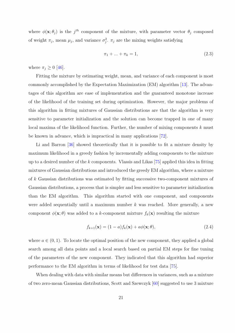
where φ(x; θj) is the jth component of the mixture, with parameter vector θj composed

of weight πj, mean µj, and variance σ2j . πj are the mixing weights satisfying

π1 + ... + πk = 1, (2.3)

where πj ≥ 0 [46].

Fitting the mixture by estimating weight, mean, and variance of each component is most

commonly accomplished by the Expectation Maximization (EM) algorithm [13]. The advan-

tages of this algorithm are ease of implementation and the guaranteed monotone increase

of the likelihood of the training set during optimization. However, the major problems of

this algorithm in fitting mixtures of Gaussian distributions are that the algorithm is very

sensitive to parameter initialization and the solution can become trapped in one of many

local maxima of the likelihood function. Further, the number of mixing components k must

be known in advance, which is impractical in many applications [72].

Li and Barron [36] showed theoretically that it is possible to fit a mixture density by

maximum likelihood in a greedy fashion by incrementally adding components to the mixture

up to a desired number of the k components. Vlassis and Likas [75] applied this idea in fitting

mixtures of Gaussian distributions and introduced the greedy EM algorithm, where a mixture

of k Gaussian distributions was estimated by fitting successive two-component mixtures of

Gaussian distributions, a process that is simpler and less sensitive to parameter initialization

than the EM algorithm. This algorithm started with one component, and components

were added sequentially until a maximum number k was reached. More generally, a new

component φ(x; θ) was added to a k-component mixture fk(x) resulting the mixture

fk+1(x) = (1− a)fk(x) + aφ(x; θ), (2.4)

where a ∈ (0, 1). To locate the optimal position of the new component, they applied a global

search among all data points and a local search based on partial EM steps for fine tuning

of the parameters of the new component. They indicated that this algorithm had superior

performance to the EM algorithm in terms of likelihood for test data [75].

When dealing with data with similar means but differences in variances, such as a mixture

of two zero-mean Gaussian distributions, Scott and Szewczyk [60] suggested to use 3 mixture

21

components and then the method of moments (MoM) to replace two of the components with

one component. A mixture of two univariate Gaussian distributions was estimated using

a 3-component mixture Gaussian, where one component had small variance with zero or

approximately zero mean and two other components had large variances and means well to

the left and to the right of the first component. The MoM was used to combine the left and

right components into one component with large variance and a mean close to zero. More

precisely, if the weight, mean, and variance of the first, second, and third component are

(w1, µ1, σ21), (w2, µ2, σ

22), and (w3, µ3, σ

23) respectively, then the second and third component

can be replaced with one component with parameters wnew = w2 + w3, µnew = w′2µ2 + w′

3µ3,

and σ2new = w′

2σ22 + w′

3σ23 + w′

2w′3(µ2 − µ3)

2, where w′2 = w2/wnew,w′

3 = 1− w′2.

2.2.6 Alternate Projections

Although the use of multiple transforms [12] was suggested to represent the musical sig-

nal more effectively, this approach relied on thresholds. It may suffer from the presence of

transient information in the tonal component and vice versa if the thresholds are selected

improperly [12]. Daudet and Torresani mentioned that one limitation of their two-step esti-

mation of the tonal and transient components is that the estimation of the tonal component

is biased by the presence of the transient and vice versa [12]. To avoid this weakness, they

suggested an alternative strategy: the so-called alternate projections [3].

With this strategy, the tonal component was first estimated using a large threshold value

resulting in a very small number of significant MDCT coefficients. The tonal component

was then estimated and subtracted from the original signal giving the non-tonal component.

The transient component was estimated from the non-tonal component by using a large

wavelet coefficient threshold value resulting in a small number of most significant wavelet

coefficients. The transient component was estimated and subtracted from the non-tonal

component leaving the residual component.

The process was repeated on the residual component; the residual component was used to

estimate the tonal and transient components iteratively until the resulting residual compo-

nent in the last iteration had a flat spectrum. The resulting tonal and transient components

22

were the sum of the tonal and transient components, respectively, from every iteration. The

residual component was the residual that resulted from the last iteration, and it was encoded

by LPC.

2.3 MEASURES OF SPEECH INTELLIGIBILITY

In speech intelligibility tests, subjects (listeners) are provided with test materials and asked

to identify them [38]. More generally, subjects may be provided with sentences, words, or

syllables and asked to write down what they hear or asked to choose one that is closest

to what they heard from several choices. Alternatively, subjects may be provided with a

paragraph and then asked to answer questions based on the contents of that paragraph.

The percentage of correct responses based on some predetermined criterion is referred to

the intelligibility or articulation score [18]. When subjects hear a particular stimulus but

response with a wrong answer, this kind of mistake is called a confusion. Confusions are

generally studied in a test, where the subjects are forced to answer to every stimulus, such

as the study of Fairbanks [20], House et al. [29], [30], and Miller and Nicely [47].

With a given type of degradation such as noise or competing speakers, the intelligibility

score is computed at different levels of degradation represented in terms of signal-to-noise

ratio (SNR). In this section, only the intelligibility of words and confusions are reviewed.

2.3.1 Word Identification in Noise

Word identification in noise has been used as a traditional measurement of speech intelligi-

bility since the works by Campbell in 1910 [5], Fletcher in 1929 [21], and Egan in 1948 [18].

Subjects were asked to identify words (stimuli), which can be either monosyllabic words or

sentences, combined with noise at different levels of signal-to-noise ratio (SNR). Different

types of noises, including white noise, speech babble, and speech-weighted noise have been

used. Word identification in noise is also referred to as a speech recognition task [40]. Speech

recognition tests can be categorized as open-set or closed-set identification tasks.

23

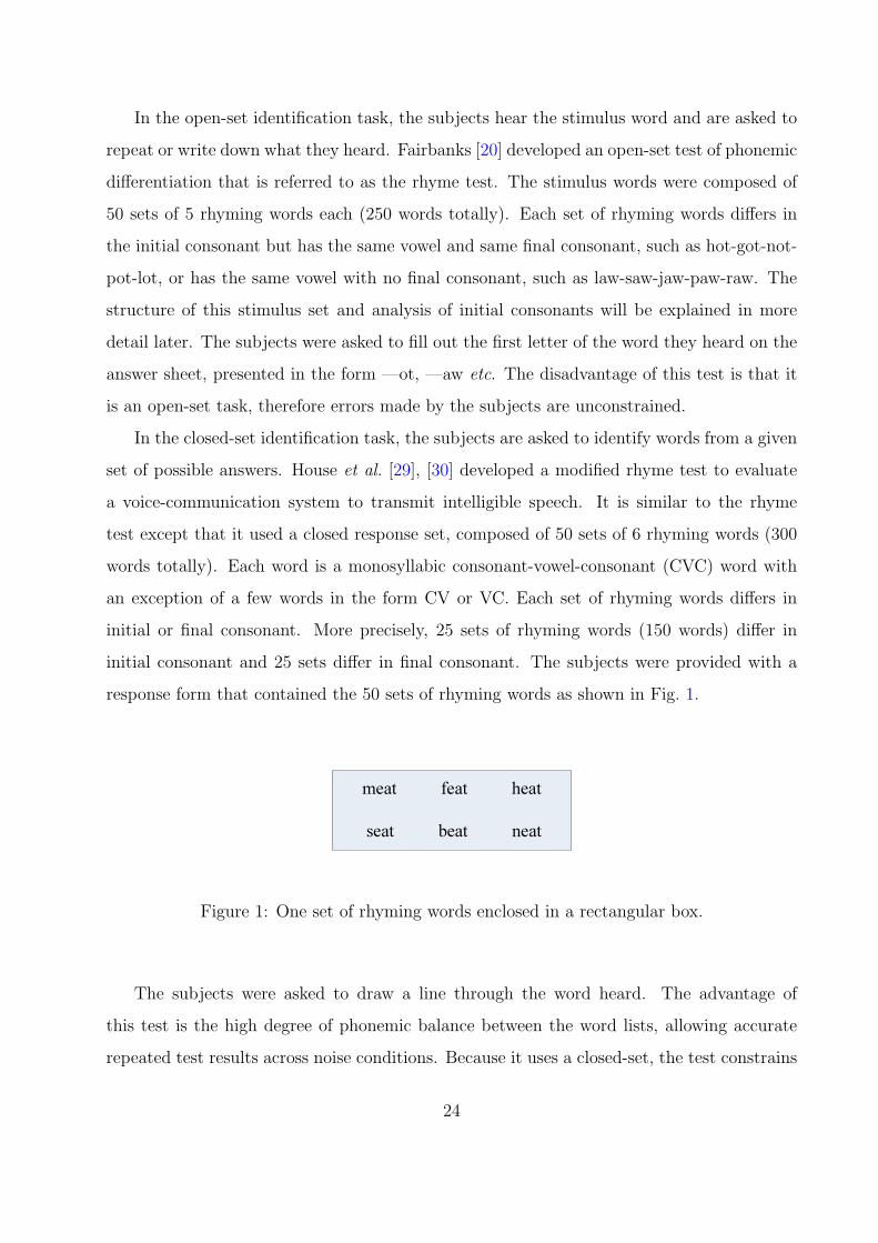
In the open-set identification task, the subjects hear the stimulus word and are asked to

repeat or write down what they heard. Fairbanks [20] developed an open-set test of phonemic

differentiation that is referred to as the rhyme test. The stimulus words were composed of

50 sets of 5 rhyming words each (250 words totally). Each set of rhyming words differs in

the initial consonant but has the same vowel and same final consonant, such as hot-got-not-

pot-lot, or has the same vowel with no final consonant, such as law-saw-jaw-paw-raw. The

structure of this stimulus set and analysis of initial consonants will be explained in more

detail later. The subjects were asked to fill out the first letter of the word they heard on the

answer sheet, presented in the form —ot, —aw etc. The disadvantage of this test is that it

is an open-set task, therefore errors made by the subjects are unconstrained.

In the closed-set identification task, the subjects are asked to identify words from a given

set of possible answers. House et al. [29], [30] developed a modified rhyme test to evaluate

a voice-communication system to transmit intelligible speech. It is similar to the rhyme

test except that it used a closed response set, composed of 50 sets of 6 rhyming words (300

words totally). Each word is a monosyllabic consonant-vowel-consonant (CVC) word with

an exception of a few words in the form CV or VC. Each set of rhyming words differs in

initial or final consonant. More precisely, 25 sets of rhyming words (150 words) differ in

initial consonant and 25 sets differ in final consonant. The subjects were provided with a

response form that contained the 50 sets of rhyming words as shown in Fig. 1.

meat feat heat

seat beat neat

Figure 1: One set of rhyming words enclosed in a rectangular box.

The subjects were asked to draw a line through the word heard. The advantage of

this test is the high degree of phonemic balance between the word lists, allowing accurate

repeated test results across noise conditions. Because it uses a closed-set, the test constrains

24

the errors made by the subjects. However, a drawback of this test is that the subjects were

forced to make responses to every stimulus set, allowing inflation of scores due to guessing

[40].

To reduce the inflation of scores problem in the closed-set identification task, Mackersie

et al. [40] developed a new word-monitoring task using the rhyming words of the modified

rhyme test [30]. The subjects listened to 50 sets of rhyming words (6 words per set), presented

at one of six SNR levels (–3, 0, 3, 6, 9, and 12 dB) of speech-weighted background noise.

Subjects were asked to identify a target word from a list of six words. The target word

appeared on the computer screen and remained until all of six words were presented. The

subjects were asked to push a button as soon as they thought that they heard the target

word. The subjects could not change an answer and could not select a previous word. This

test is expected to be less susceptible to score inflation because the subjects are not forced

to answer to every stimulus set. The subjects did not see the alternatives before they were

presented, as in the modified rhyme test protocol [30].

Yoo [77] used the modified rhyme protocol, developed from House et al. [30] and Mack-

ersie et al. [40], to compare the intelligibility of a form of enhanced speech to original speech.

The protocol was performed on eleven volunteer subjects with negative otologic histories and

hearing sensitivity of 15 dB HL or better by conventional audiometry (250 - 8 kHz). Fifty

sets of rhyming monosyllabic CVC words (6 words per set for a total of 300 words), were

recorded by a male speaker [77]. Among them, 25 sets differed in their initial consonants

and 25 sets differed in their final consonants.

Subjects sat in a sound-attenuated booth and were asked to identify a target word from

a list of six words. The target word appeared on the computer screen and remained until all

six words were presented. These six words were presented through the right headphone at

one of six SNR levels (–25, –20, –15, –10, –5, and 0 dB) using speech-weighted background

noise. The subjects were asked to click a mouse as soon as they thought that they heard the

target word. The subjects could not change an answer and could not select a previous word.

25

2.3.2 Consonant Confusions in Noise

Confusions of speech sounds in noise have been studied for several decades. Most studies

have investigated confusions of consonants in initial position [20], [47] or in initial and final

positions [30].

Miller and Nicely [47] investigated confusions of 16 initial consonants including /p/, /t/,

/k/, /f/, /T/, /s/, /S/, /b/, /d/, /g/, /v/, /D/, /z/, /Z/, /m/, and /n/. They suggested

that these consonants constitute almost three quarters of normal speech and about 40 per-

cent of all phonemes with vowels included. Two hundred words that differ in these initial

consonants followed by a vowel /A/ were used as stimulus words and were spoken over voice

communication systems with 17 different frequency distortions and random masking noises.

Five female subjects were used in their studies. In each test condition, one subject served

as a talker, and the other four subjects served as listeners. The listeners were asked to write

down an answer to every stimulus. Therefore, with 4 listeners, there were 800 responses for

each talker. In total, there were 4,000 responses in each test condition and each consonant

occurred 250 times.

Responses of each test were counted and represented in the so-called confusion matrix,

where each row represents the stimulus consonant and each column represents the response

consonant. The number in each cell is the frequency of occurrence of the response consonant

corresponding to the column to the stimulus consonant corresponding to the row. Each

diagonal element represents the frequency of correct responses, and off diagonal elements

represent incorrect responses.

Miller and Nicely found that with various degrees of masking noise (–18, –12, –6, 0, 6,

and 12 dB with bandwidth 200-6,500 Hz), the confusions had a consistent pattern. The

confusions were randomly scattered at SNR of –18 dB. The frequency of correct responses

(diagonal elements) started to increase with increasing SNR, while confusions began to be

emphasized in consonants categorized within the same group i.e. /ptk/ (voiceless plosive con-

sonants), /fTsS/ (voiceless fricative consonants), /bdg/ (voiced plosive consonants), /vDzZ/

(voiced fricative consonants), and /mn/ (nasal). The confusions (off diagonal elements) were

26

reduced dramatically, especially in consonants categorized in different groups (most of them

were zero) at 12 dB. At this SNR level, the confusion matrix were dominated by diagonal

elements with some confusions of consonants categorized within the same group.

With various low-pass filters (resulting in bandwidth 200 to 300, 200 to 400, 200 to 600,

200 to 1200, 200 to 2500, and 200 to 5000 Hz at 12 dB masking noise level), similar results as

in the case of masking noise effects were found. With various high-pass filters (resulting in

bandwidth 200 to 5000, 1000 to 5000, 2000 to 5000, 2500 to 5000, 3000 to 5000, and 4500 to

5000 Hz), the errors did not cluster or show a consistence pattern as in the case of masking

noise and low-pass filtering effects. The confusions in this case were scattered randomly.

Miller and Nicely concluded that although low-pass filtering affected linguistic features,

it had limited effect on the audibility of consonants. On the other hand, high-pass filtering

removed most of acoustic power in the consonants, making them inaudible and producing

random confusions [47].

As stated earlier, Fairbanks [20] developed the rhyme test to investigate cues for responses

of the initial consonants and consonant-vowel transitions. Fifty sets of 5 rhyming words (250

words total) were generated from 18 consonants (/s/, /t/, /b/, /m/, /l/, /p/, /r/, /w/, /k/,

/h/, /f/, /d/, /n/, /g/, /dZ/, /v/, /j/, and /z/). Instead of using one vowel (/A/) as in

Miller and Nicely [47], Fairbanks used 13 vowels, including /I/, /e/, /E/, /A/, /AI/, /2/, /i/,

/æ/, /O/, /Ú/, /u/, /o/, and /OI/. One advantage of this protocol is that it allowed him to

investigate consonant-vowel transitions. Each of 5 rhyming words in each set was randomly

assigned to one of five word lists, so that each word list was composed of 50 stimulus words.

Forty subjects were used in Fairbanks’s study. He divided the subjects into 2 groups

(20 subjects each) referred to as groups A and B. Each group was divided further into 5

subgroups (4 subjects each). Five vowel-to-noise (V/N) ratios (–6, –4, –2, 0, and 2 dB) were

used in group A. For a given subgroup, one word list was assigned to each V/N ratio. A

Latin square design was used to assign word lists to V/N ratios such that all stimulus words

and all subjects were represented equally at each V/N ratio. Therefore, each subject heard

the complete set of stimulus words (250 words) once. For group B, the same method was

used except that different V/N ratios (–2, 1, 5, 9, and 15 dB) were used.

27

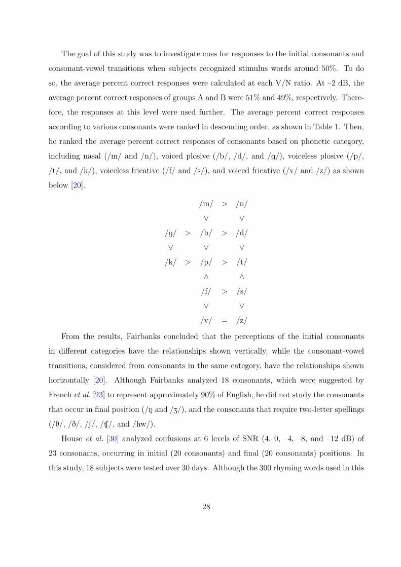
The goal of this study was to investigate cues for responses to the initial consonants and

consonant-vowel transitions when subjects recognized stimulus words around 50%. To do

so, the average percent correct responses were calculated at each V/N ratio. At –2 dB, the

average percent correct responses of groups A and B were 51% and 49%, respectively. There-

fore, the responses at this level were used further. The average percent correct responses

according to various consonants were ranked in descending order, as shown in Table 1. Then,

he ranked the average percent correct responses of consonants based on phonetic category,

including nasal (/m/ and /n/), voiced plosive (/b/, /d/, and /g/), voiceless plosive (/p/,

/t/, and /k/), voiceless fricative (/f/ and /s/), and voiced fricative (/v/ and /z/) as shown

below [20].

/m/ > /n/

∨ ∨/g/ > /b/ > /d/

∨ ∨ ∨/k/ > /p/ > /t/

∧ ∧/f/ > /s/

∨ ∨/v/ = /z/

From the results, Fairbanks concluded that the perceptions of the initial consonants

in different categories have the relationships shown vertically, while the consonant-vowel

transitions, considered from consonants in the same category, have the relationships shown

horizontally [20]. Although Fairbanks analyzed 18 consonants, which were suggested by

French et al. [23] to represent approximately 90% of English, he did not study the consonants

that occur in final position (/N and /Z/), and the consonants that require two-letter spellings

(/T/, /D/, /S/, /Ù/, and /hw/).

House et al. [30] analyzed confusions at 6 levels of SNR (4, 0, –4, –8, and –12 dB) of

23 consonants, occurring in initial (20 consonants) and final (20 consonants) positions. In

this study, 18 subjects were tested over 30 days. Although the 300 rhyming words used in this

28

test were not phonetically balanced, these rhyming words include the major categories of

speech sounds in English [30]. Frequency of occurrences of the stimulus consonants in the

test set are summarized in Table 2.

House et al. found that most consonantal elements in initial position were recognized more

successfully than consonantal elements in final position. In addition, voiceless consonants

were recognized more successfully than voiced consonants (/p/ > /b/, /f/ > /v/, and /t/

> /d/). They also found that the average percent correct responses of each consonantal

element were ranked inversely compared with the results of Fairbanks [20].

Specifically, Fairbanks found that at the level of 50% identification, nasal consonants /m/

and /n/ were recognized at the highest rate, while /s/, /p/, and /t/ were poorly recognized

[20]. House et al. found the opposite [30]. The average percent correct responses according

to phonetic elements of House et al. are summarized in Table 3. House et al. suggested that

the difference was due to the different characteristics of noises used in their study and in

the Fairbanks study. The Fairbanks study used a uniform (white) noise, which might have

masked the high-frequency information associated with voiceless consonants more effectively3

than the speech-weighted noise used in their study [30].

2.4 SUMMARY

Speech enhancement is to improve the performance of communication systems, where their

input or output speech is degraded by background noise [19]. When dealing with speech

enhancement, two criteria can be considered — quality and intelligibility. Quality is a sub-

jective measure, while the intelligibility is an objective measure. These two measures are

independent i.e. a given speech signal can possibly have high quality but have low intelligi-

bility, and vice versa [19].

The objective of speech enhancement is to improve the overall quality, to increase the

intelligibility, or to reduce listener fatigue [38]. Speech enhancement also depends on specific

3Since the hearing organ looks roughly like a constant-percentage bandwidth filtering bank at high fre-quency.

29

applications i.e. one application may deal only with one of these objectives, but another

application may deal with several objectives. Speech enhancement can be divided into 2

categories. The first category is to deal with enhancement of speech already degraded by

noise, and the second category is to deal with enhancement of clean speech before it is

degraded by noise [19].

Regardless of noise types, enhancement of speech already degraded by noise was investi-

gated at higher SNR levels compared to enhancement of the clean speech before it is degraded

by noise. More precisely, 0 - 10 dB [70], –8 - 4 dB [16], –3 - 9 dB [55], and –5 - 5 dB [37]

were the SNR levels investigated in the studies belonged to the first category, while lower

SNR levels i.e. –10 - 10 dB [50], [68], and –25 - 0 dB [77] were investigated in the studies

belonged to the second category. This may imply that speech enhancement of clean speech

before it is degraded by noise can be effectively applied to the application in higher levels of

background noise.

Several approaches to increase the intelligibility of speech already contaminated by noise

(noisy speech) have been proposed but these approaches have limitations and/or disadvan-

tages when they are used in real situations. These can be explained as follow. The quality of

the enhanced speech was worse than that of the noisy speech [38] in the approach of Thomas

and Ravindran [70]; the locations of the phoneme /s/ and the plosive sounds were assumed

to be accurately located in order to apply high-pass filtering to the phoneme /s/ and to add

short pauses before occurrence of the stop sounds in the approach of Drucker [16]; accurate

pitch information, which cannot be expected to be obtained from the noisy speech [38], was

assumed to be available in the approach based on the use of comb filtering of Shields [62]

and the approach based on the use of adaptive comb filtering of Frazier et al. [22].

Approaches to increase the intelligibility of clean speech before it is corrupted by noise are

based on either high-pass filtering alone [69] or high-pass filtering followed by other methods

i.e. infinite clipping [68], amplitude compression [50], time-varying bandpass filtering [77].

The high-pass filtering was used because the first formant frequency contains very low

intelligibility compared to the second formant, which contains a major part to convey the

intelligibility of speech [67]. The infinite clipping approach was used to increase the power

of the consonants and weak speech events relative to the vowels [68]. However, Niederjohn

30

and Grotelueschen [50] concluded that clipping produced harmonic distortion in the clipped

waveform and this distortion has frequency components in the second and higher formant

frequencies, resulting in the signal distortion heard by listeners [50]. They suggested another

approach without introducing the distortion produced by the infinite amplitude clipping.

That approach is amplitude compression [68]. Yoo [77] applied three time-varying bandpass

filters following high-pass filtering to extract transient information, which is believed to

be critical to speech perception. The transient component was selectively amplified and

recombined to the original speech to generate enhanced speech, with energy was adjusted to

be equal to that of the original speech.

The psychoacoustic test results of Yoo [77] evaluated lower SNR levels (–25, –20, –15, –

10, –5, and 0 dB) compared with other studies [50], [68] and showed substantial improvement

in the intelligibility of the enhanced speech compared with the original speech at SNR –25

dB, –20 dB, and –15 dB. However, the resulting transient component retained a significant

amount of energy during what would appear to be tonal portions of the speech [65], and

Yoo’s approach relied on high-pass filtering, which has been shown to enhance speech in noise

[50], [67], [68], [69]. Therefore, improvement of intelligibility of speech in noise of Yoo [77]

may have, at least in part, come from the effect of increasing the relative power of formant

frequency information in high frequency ranges.

Because the transient component in speech is not well defined, we have been developing

another approach to identify the transient component in speech. The specific proposed

changes to improve transient identification in speech over Yoo’s algorithm [77] are to include

transient information in the low frequency region and to reduce the amount of voicing (tonal)

energy in the transient.

Word identification in noise [5], [18], [21] or speech recognition task [40] has been used as

an approach to measure speech intelligibility quantitatively. It can be divided into an open-

set and closed-set identification task. In the open-set identification task, subjects hear the

stimulus and are asked to repeat or write down what they heard. The disadvantage of this

test is that errors made by the subjects are unconstrained. In the closed-set identification

task, subjects are asked to identify words from a given set of possible answers. The advantage

of this test is that it constrains the errors made by the subjects, but a drawback is that the

31

subjects are forced to response to every stimulus set, allowing inflation of scores because of

guessing [40]. A word-monitoring task [40] is suggested to be less susceptible to score inflation

because the subjects are not forced to answer to every stimulus set. In this task, the target

word appears on the computer screen and remains until all of six words are presented. The

subjects are asked to push a button as soon as they think that they heard the target word.

When subjects hear a particular stimulus but responds with a wrong answer, this kind

of mistake is called a confusion. Generally, confusions have been studied in a test, where

the subjects were forced to answer to every stimulus [20], [30], [47]. Consonant confusions in

noise have been investigated in several studies i.e. in initial consonant [20], [47] and initial

and final consonants [29], [30]. A confusion matrix has been used to reveal confusions of the

subjects represented as off diagonal elements, while diagonal elements represent consonants

correctly recognized by the subjects.

32

Table 1: Average percent correct responses according to various consonants at V/N = –2

dB from Table VI of Fairbanks [20].

% Correct

/m/ 76.2

/n/ 62.3

/j/ 62.3

/g/ 61.1

/f/ 59.2

/l/ 55.9

/b/ 52.3

/w/ 52.2

/r/ 49.3

/k/ 44.5

/d/ 43.3

/Ã/ 40.6

/s/ 40.3

/p/ 40.3

/h/ 39.8

/t/ 38.6

/v/ 25.0

/z/ 25.0

33

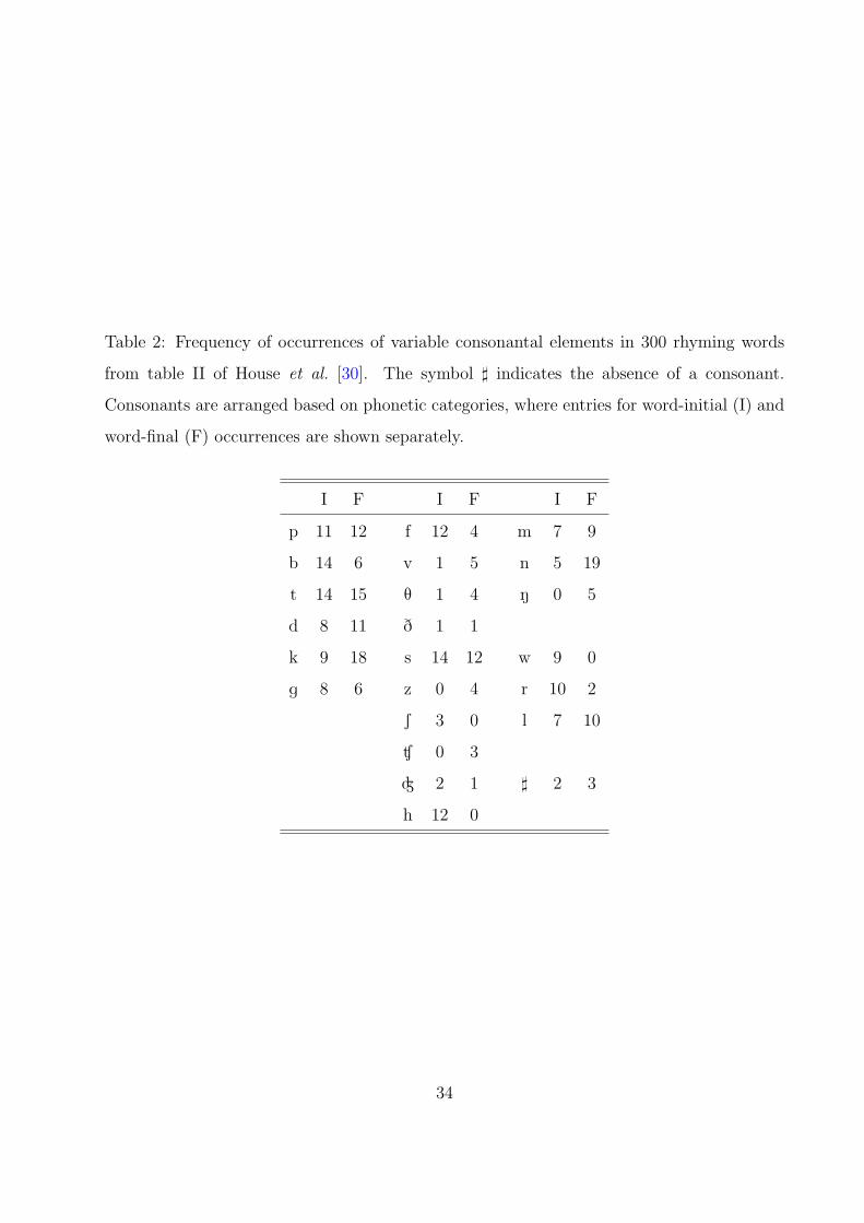
Table 2: Frequency of occurrences of variable consonantal elements in 300 rhyming words

from table II of House et al. [30]. The symbol ] indicates the absence of a consonant.

Consonants are arranged based on phonetic categories, where entries for word-initial (I) and

word-final (F) occurrences are shown separately.

I F I F I F

p 11 12 f 12 4 m 7 9

b 14 6 v 1 5 n 5 19

t 14 15 T 1 4 N 0 5

d 8 11 D 1 1

k 9 18 s 14 12 w 9 0

g 8 6 z 0 4 r 10 2

S 3 0 l 7 10

Ù 0 3

à 2 1 ] 2 3

h 12 0

34

Table 3: Average percent correct response according to phonetic elements from table V

of House et al. [30]. The symbol ] indicates the absence of a consonant. Consonants are

arranged based on phonetic categories, where entries for word-initial (I) and word-final (F)

occurrences are shown separately.

I F I F I F

p 82 56 f 86 74 m 67 38

b 72 57 v 61 65 n 66 64

t 91 79 T 81 56 N - 57

d 75 64 D 66 44

k 83 65 s 98 96 w 79 -

g 77 70 z - 91 r 69 68

S 61 - l 71 74

Ù - 83

à 85 69 ] 70 79

h 70 -

35

3.0 SPEECH DECOMPOSITION METHOD AND RESULTS

3.1 OVERVIEW

Daudet and Torresani [12] decomposed a musical signal into tonal, transient, and residual

components using the modified discrete cosine transform (MDCT) and the wavelet transform.

The MDCT provides good estimates of locally stationary signals [12]. The tonal component

was estimated by the inverse transform of a small number of MDCT coefficients whose

absolute values exceed a selected threshold. The tonal component was subtracted from the

original signal to obtain what they defined as the non-tonal component. The non-tonal

component was transformed using the wavelet transform, which provides good results in

encoding signals with abrupt temporal changes [12]. The transient component was estimated

by the inverse of the wavelet transform, using a small number of wavelet coefficients whose

absolute values exceed another selected threshold. The residual component, obtained by

subtracting the transient component from the non-tonal component, was expected to be a

stationary random process with a flat spectrum.

The significant MDCT and wavelet coefficients were separately quantized and entropy

encoded. The residual component was estimated using standard linear prediction coding

(LPC) and the filter coefficients were quantized and encoded. The final bit rate of the

musical signal was the sum of bit rates used to code the tonal, transient, and residual

components.

Our modifications of this algorithm involved two aspects. First, we wanted to avoid

a threshold, since an appropriate value is not known. Our goal was to isolate a transient

component, and we were not concerned with coding rate per se. Second, we wanted to

incorporate statistical dependencies in the MDCT coefficients as well as in the wavelet coef-

36

ficients, which were assumed to be independent by Daudet and Torresani [12]. Specifically,

Crouse et al. [8] have suggested that the wavelet coefficients have clustering and persistence

properties, and so do the MDCT coefficients, as suggested by Daudet et al. [10].

Crouse et al. [8] developed a probabilistic model to capture complex dependencies and

non-Gaussian statistics of the wavelet transform. They used the model, called the hidden

Markov tree (HMT) model, to describe the statistical dependencies of the wavelet coefficients

along and across scale, based on clustering and persistence properties, by utilizing Markov

dependencies. They modeled the wavelet coefficients as a two-state, zero-mean Gaussian

mixture, where “large” states and “small” states were associated with large variance and

small variance, zero-mean Gaussian distributions, respectively. The wavelet coefficients were

observed but the state variables were hidden. They also introduced the upward-downward

algorithm for training the model.

Molla and Torresani [48] applied the HMT model [8] to estimate the transient component

in a musical signal. They associated the transient state with a large-variance Gaussian dis-

tribution and the residual state with a small-variance Gaussian distribution. They used the

statistical inference method [17], which is more robust than the upward-downward algorithm

to the numerical underflow problem.

Daudet et al. [10] proposed a probabilistic model to estimate the tonal component in

a musical signal. They applied a hidden Markov chain (HMC) model [57] to describe the

statistical dependencies of the MDCT coefficients in each frequency index. They modeled

the MDCT coefficients as a two-state, zero-mean Gaussian mixture. A tonal state was

associated with a large-variance Gaussian distribution, and a non-tonal state was associated

with a small-variance Gaussian distribution.

One important issue when dealing the HMC and HMT models is estimates of the initial

values of mixtures of two univariate Gaussian distributions. The most popular algorithm used

to estimate parameters of a mixture of Gaussian distributions is Expectation Maximization

(EM) [13]. However, this algorithm is not guaranteed to converge to a globally optimal

solution. The main problem in fitting mixtures of Gaussian distributions is that the algorithm

is very sensitive to parameter initialization, and the solution can become trapped in one of

many local maxima of the likelihood function [72]. Vlassis and Likas [75] proposed the greedy

37

EM algorithm, which starts with a single component. Components are added sequentially

until reaching a maximum number k. This algorithm showed superior performance to the

EM algorithm in terms of likelihood [75].

When dealing with data with similar means but differences in variances, such as a mixture

of two zero-mean Gaussians. Scott and Szewczyk [60] used an approach based on average

shifted histogram (ASH) density estimate [59] and suggested using 3 mixture components and

then the method of moments (MoM) to replace two of the components with one component.

Our method has been developed from the approaches of Daudet and Torresani [12], Molla

and Torresani [48], and Daudet et al. [10], where these approaches were intended to achieve a

low bit rate with minimum perceived loss in encoding a musical signal. These researchers did

not describe the performance of their methods specifically to identify a transient component

in speech. However, to the extent that these methods improve coding efficiency by an

effective decomposition of the signal into tonal and transient components, we believe that

these methods may provide an effective means to identify a transient component.

The hidden Markov chain (HMC) model and the hidden Markov tree (HMT) model

are applied to capture statistical dependencies, assumed to be independent in Daudet and

Torresani [12], between the MDCT coefficients and between the wavelet coefficients, respec-

tively. The Viterbi algorithm [57] and the MAP algorithm [17] are applied to find the optimal

state distribution of the MDCT and the wavelet coefficients that result in determinations of

the significant MDCT and wavelet coefficients automatically without relying on threshold

as does Daudet and Torresani [12].

The MDCT and the wavelet coefficients are modeled as a non-zero mean Gaussian mix-

ture instead of a zero mean Gaussian mixture as do Daudet et al. [10] and Molla and Torresani

[48]. The non-zero mean model allows better fit of the model to the data. We believe that

this better fit provides more effective identification of the tonal and transient components.

The greedy EM algorithm [75], suggested to be less sensitive to initial parameter initial-

ization than the EM algorithm [13], is applied to estimate initial parameters (means and

variances) of the HMC and HMT modeled as a mixture of two univariate Gaussian distribu-

tions. We believe that with better initializations of the models, more effective estimations

of the tonal and transient components can be obtained.

38

Details of our method are described in Section 3.2. This section is composed of a brief

review of the MDCT, window length selection of the MDCT, investigation of the greedy EM

algorithm using 2-component and 3-component models and then the MoM, tonal estimation,

a brief review of the wavelet transform, transient estimation, and the use of the residual

component from the first iteration based on the idea of alternate projection [3].

The original speech signal is expanded using the MDCT, and the HMC model [57] is

manipulated to identify the tonal component. The non-tonal component is decomposed using

the wavelet transform, and the HMT model [8] and the statistical inference method [17] are

applied to identify the transient component. The optimal state distribution of the MDCT

and wavelet coefficients are determined by the Viterbi algorithm [57] and the Maximum a

posteriori (MAP) algorithm [17], respectively. Transitions and abrupt temporal changes in

speech are expected to be included in the transient component. The decomposition results

on the words “pike” and “got” are illustrated and explained in detail in Section 3.3. Finally,

our method is summarized in Section 3.4.

3.2 SPEECH DECOMPOSITION ALGORITHM

3.2.1 The Modified Discrete Cosine Transform (MDCT)

The MDCT was introduced by Princen and Bradley [54] based on the concept of time domain

aliasing cancelation (TDAC). It is a Fourier-related transform, based on the type-IV discrete

cosine transform (DCT-IV) [41]. It is also referred to as the perfect reconstruction (PR)

cosine modulated filter bank with some restrictions on the window w(n) [52].

Painter [52] summarized the MDCT from the perspective of an analysis-synthesis filter

bank as shown in Fig. 2. The MDCT analysis filter impulse responses can be expressed as

hk(n) = w(n)

√2

Mcos

[(2n + M + 1)(2k + 1)π

4M

]. (3.1)

In the forward MDCT, the input signal, x(n), is divided into frames (each frame with

length M samples). Then, a block transform of length 2M samples, composed of M samples

39

from frame m and M samples from frame m + 1 (advanced frame), are used in the analysis

filter bank with 50% overlap between blocks. More precisely, the MDCT basis function

is extended across two frames (2M samples) in time, but only M samples are generated,

i.e. given an input block, x(n), the transform coefficients (MDCT coefficients) in each time

frame, X(k), can be expressed as

X(k) =2M−1∑n=0

x(n)hk(n), 0 ≤ k ≤ M − 1. (3.2)

From (3.2), the forward MDCT is a series of inner products between the M analysis filter

impulse responses hk(n) and the input signal x(n).

In the inverse MDCT, a reconstructed signal is obtained by computing a summation of

the basis vectors, weighted by the MDCT coefficients from 2 blocks. More precisely, the first

M samples of the kth basis vector hk(n), for 0 ≤ n ≤ M−1, are weighted by the kth MDCT

coefficient of the current block, and the second M samples of the kth basis vector hk(n), for

M ≤ n ≤ 2M − 1, are weighted by the kth MDCT coefficient of the previous block XP (k)

[52]. As a result, the weighted basis vectors are overlapped and added at each time frame

m. The reconstructed signal, x(n), in each time frame can be expressed as

x(n) =M−1∑

k=0

[X(k)hk(n) + XP (k)hk(n + M)

], 0 ≤ n ≤ M − 1. (3.3)

The window w(n) used for the MDCT must have the two following properties:

w(2M − 1− n) = w(n) and

w2(n) + w2(n + M) = 1, where 0 ≤ n ≤ M − 1.(3.4)

One example of the MDCT window, which is probably the most popular in audio coding

[52], is the sine window used in the modulated lapped transform (MLT) [44]. This window

can be expressed as

w(n) = sin

[(n +

1

2

) π

2M

]. (3.5)

Referred to Fig. 2a, each vector of the output of the lapped forward transform (analysis)

is composed of M spectral components from frequency index 0 to M − 1, where M is equal

40

to the number of samples of the half window length. Each vector refers to one time frame.

Therefore, when considering all time frames concatenated to each other from the first to the

last time frame, the MDCT coefficients can be represented as the tiling of the time-frequency

plane illustrated in Fig. 3 (note that the total number of time frames is calculated from the

length of signal divided by the half-window length). Each black node represents a particular

MDCT coefficient in time-frequency representation. Based on an approach of Daudet and

Torresani [12], the tonal component was identified by the inverse transform of all of black

nodes (significant MDCT coefficients) whose absolute values exceeded a threshold value.

3.2.2 Window Length Selection

The window length of the MDCT is crucial. It should be short enough such that the resulting

tonal component in each time frame is reasonably modeled as a locally stationary signal, and

it should be long enough to ensure sufficient frequency resolution [12].

In addition, the chosen window length is expected to suppress or to minimize pre-echo

distortion as much as possible. The pre-echo distortion is an artifact that is seen as fluctu-

ations in waveform amplitude. These artifacts usually occur in the estimation of the tonal

component because the resulting tonal component is generated based on the idea of trans-

form coding (i.e. using a small number of significant MDCT coefficients) [11]. The artifacts

occur especially in the area where the sharp attack of the original signal begins near the end

of the transform block and that attack is immediately followed by a low energy part of the

original signal [52].

To find an appropriate window length to use in this project, several window lengths

were investigated. Based on preliminary results and informal listening tests on the word

“pike”, 40 CVC words from NU-6 [71], and 300 rhyming words used in the psychoacoustic

test of Yoo [77], we found that the half window length 23.2 ms, which was used in Daudet

and Torresani [12], gave a good frequency resolution, but the resulting tonal component

appeared to include pre-echo distortion not occurring in the original speech.

Figure 4 illustrates time and spectrogram plots of the word “pike”. Figure 5 illustrates

time and spectrogram plots of the resulting tonal component using a half-window length

41

23.2 ms (256 samples at 11.025 kHz sampling frequency). The pre-echo distortion is clearly

seen in both time and spectrogram plots. This pre-echo distortion degraded the quality

of the tonal component, making it sound similar to speaking through a pipe. Therefore,

shorter half window lengths were investigated (the half-window length has to have its length

to be a power of 2). The half window length 11.6 ms (128 samples) was investigated. The

pre-echo distortion was reduced compared with the case using 23.2 ms half window length

but artifacts are still remarkable.

The half window length 1.5 ms (16 samples) minimizes the pre-echo distortion but it

is too short to provide good frequency resolution. This can be seen in the resulting tonal

component illustrated in Fig. 6. When considering the resulting tonal component around the

area A in both time and spectrogram plots, it is clear that only part of the constant formant

frequency information was captured compared with the same area of the original speech. In

addition, part of that constant formant frequency information is broad in frequency. This

broad frequency information is also found in areas B and C, which is not considered as a

locally stationary signal.

We found the half window length 2.9 ms (32 samples) to be long enough to ensure suffi-

cient frequency resolution. This length is short enough that the resulting tonal component

in each time frame is reasonably modeled as a locally stationary signal. The resulting tonal

component using this half-window length is illustrated in Fig. 7. When considering the re-

sulting tonal component around the area A, it is clear that most of the constant formant

frequency information was captured compared with the same area of the original speech.

The tonal component around the area A does not spread over frequency as in the case of the

1.5 ms half window length. In addition, spread over frequency of tonal information in areas

B and C was dramatically reduced.

Therefore, the sine window with half-window length 2.9 ms shown in Fig. 8 was used

in this project. This finding supported the suggestion of Painter [52] that when pre-echo

distortions are likely to appear, a short window (i.e. 2-5 ms) should be used to localize

time-domain artifacts.

42

3.2.3 Estimation of Gaussian Distribution Parameters

The greedy EM algorithm is used to estimate parameters (means and variances) of a mixture

of two univariate Gaussian distributions, where each distribution has similar means but

differences in variances. Scott and Szewczyk [60] suggested to use 3 mixture components and

then the method of moments (MoM) to replace two of the components with one component.

To investigate performances of parameter estimations using 2-component mixture Gaussian

and 3-component mixture Gaussian and then the MoM, a Monte Carlo simulation was used

to generate 10 data sets [15], [28], where each data set is composed of 128 data points

from a mixture of two univariate Gaussian distributions with known parameters (weights,

means, and variances). Data sampled from a Gaussian mixture were generated by a Matlab

function “gmmsamp” from a statistical pattern recognition toolbox for Matlab1. The known

parameters are weights (w1 = 0.6, w2 = 0.4), means (µ1 = 0, µ2 = 0), and variances (σ12 =

10−6, σ22 = 10−3). Based on preliminary results on speech signals, these parameter values

closely correspond to the parameters estimated from the MDCT coefficients in each frequency

index and the wavelet coefficients in each tree.

The greedy EM algorithm was used to fit each data set using the 2-component mixture

Gaussian shown in Fig. 9 and the 3-component mixture Gaussian shown in Fig. 10 followed by

combination using the MoM. Average parameter estimates for 10 data sets were calculated,

and mean square error (MSE) was used to compare performances between two approaches.

Tables 4 and 5 summarize parameter estimates using these two approaches. Parameter

estimates using the 2-component greedy EM algorithm were more accurate than using 3-

component greedy EM algorithm followed by the MoM, as shown by smaller MSE values.

Only MSE of µ2 using 3-component greedy EM algorithm followed by the MoM is slightly

smaller than MSE of µ2 using 2-component greedy EM algoirthm. The MSE for all other

parameters was smaller for the 2-component model.

We concluded that the 3-component method does not have an advantage for parameter

estimates of a mixture of two univariate Gaussian distributions with means not well sep-

arated, when fitting a mixture Gaussian was performed using the greedy EM algorithm.

1available at http://cmp.felk.cvut.cz/∼xfrancv/stprtool/

43

Therefore, in this project, the initial values of parameters (means and variances) of the mix-

ture of two univariate Gaussian distributions of the MDCT coefficients in each frequency

index and the wavelet coefficients in each scale of each tree are estimated using 2-component

greedy EM algorithm.

44

M

2M

M M M

2M

2M

M

M

M

MDCT

MDCT

MDCT

Frame m Frame m+1 Frame m+2 Frame m+3

M

M

M

IMDCT

IMDCT

IMDCT

2M

2M

2M

M M

+

+

Frame m+1 Frame m+2

. . . . . .

(a)

(b)

Figure 2: MDCT (a) lapped forward transform (analysis) — 2M samples are mapped to

M spectral components. (b) Inverse transform (synthesis) — M spectral components are

mapped to a vector of 2M samples From Fig. 15 of Painter [52].

45

Frequency Index

Time Frame

1 2 3 4 5 6 7 8 9 10 11 . . . ����������� �����������������

0

1

2

3

.

.

.

����������� �!"�#$%

Figure 3: Tiling of the time-frequency plane by the atoms of the MDCT.

46

0 0.1 0.2 0.3 0.4 0.5 0.6 0.7

−0.6

−0.4

−0.2

0

0.2

0.4

0.6

Original speech

ampl

itude

time (sec)

freq

(H

z)

time (sec)0 0.1 0.2 0.3 0.4 0.5 0.6 0.7

0

1000

2000

3000

4000

5000

Figure 4: Time and spectrogram plots of “pike”: click to hear the sound.

47

0 0.1 0.2 0.3 0.4 0.5 0.6 0.7

−0.6

−0.4

−0.2

0

0.2

0.4

0.6

Tonal component using half window length 23.2 ms

ampl

itude

time (sec)

freq

(H

z)

time (sec)0 0.1 0.2 0.3 0.4 0.5 0.6 0.7

0

1000

2000

3000

4000

5000

artifacts

artifacts

artifacts

artifacts

Figure 5: Time and spectrogram plots tonal component of “pike” with half window length

23.22 ms: click to hear the sound.

48

0 0.1 0.2 0.3 0.4 0.5 0.6 0.7

−0.6

−0.4

−0.2

0

0.2

0.4

0.6

Tonal component using half window length 1.5 ms

ampl

itude

time (sec)

freq

(H

z)

time (sec)0 0.1 0.2 0.3 0.4 0.5 0.6 0.7

0

1000

2000

3000

4000

5000

A

A

B

C

Figure 6: Time and spectrogram plots tonal component of “pike” with half window length

1.5 ms: click to hear the sound.

49

0 0.1 0.2 0.3 0.4 0.5 0.6 0.7

−0.6

−0.4

−0.2

0

0.2

0.4

0.6

Tonal component using half window length 2.9 ms

ampl

itude

time (sec)

freq

(H

z)

time (sec)0 0.1 0.2 0.3 0.4 0.5 0.6 0.7

0

1000

2000

3000

4000

5000

A

A

B

C

Figure 7: Time and spectrogram plots tonal component of “pike” with half window length

2.9 ms: click to hear the sound.

50

0 10 20 30 40 50 600

0.1

0.2

0.3

0.4

0.5

0.6

0.7

0.8

0.9

1

Sample (n)

Am

plitu

de

Sine window with length 64 samples (5.8 ms at sampling frequency 11.025 kHz)

Figure 8: Sine window with length 64 samples (5.8 ms at sampling frequency 11.025 kHz).

51

−0.1 −0.08 −0.06 −0.04 −0.02 0 0.02 0.04 0.06 0.08 0.10

50

100

150

200

250

True mixture GaussiansEstimated using greedy EM

Figure 9: Fitting 2 mixture Gaussians using 2-component greedy EM algorithm.

52

−0.1 −0.08 −0.06 −0.04 −0.02 0 0.02 0.04 0.06 0.08 0.10

50

100

150

200

250

True mixture GaussiansEstimated using greedy EM

Figure 10: Fitting 2 mixture Gaussians using 3-component greedy EM algorithm.

53

Table 4: Parameter estimates using 2-component greedy EM algorithm.

Parameter True value Average estimates Variance estimates MSE

w1 0.6 0.600807 0.000887 0.000799

w2 0.4 0.399193 0.000887 0.000799

µ1 0 1.616590×10−5 1.098400×10−8 1.0147×10−8

µ2 0 -0.000797 6.113850×10−6 6.138100×10−6

σ1 10−6 1.058100×10−6 1.322510×10−14 1.527600×10−14

σ2 10−3 0.0001019 1.070020×10−8 9.999600×10−9

Table 5: Parameter estimates using 3-component greedy EM algorithm and MoM.

Parameter True value Average estimates Variance estimates MSE

w1 0.6 0.439709 0.075126 0.093306

w2 0.4 0.560292 0.075126 0.093306

µ1 0 -0.000129 1.425460×10−6 1.299600×10−6

µ2 0 -0.000527 4.446120×10−6 4.279400×10−6

σ1 10−6 7.452580×10−7 2.460250×10−13 2.863100×10−13

σ2 10−3 0.000858 9.894100×10−8 1.090900×10−7

54

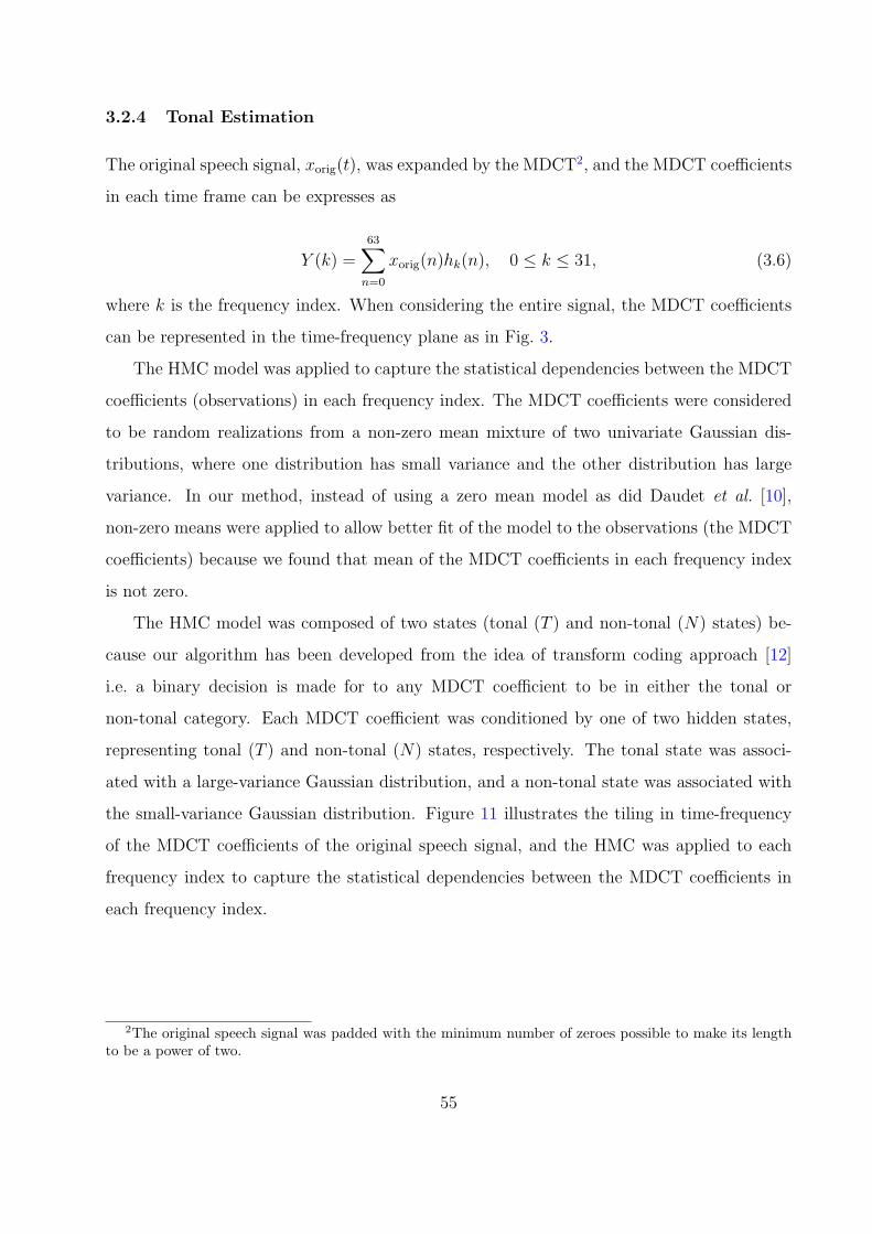
3.2.4 Tonal Estimation

The original speech signal, xorig(t), was expanded by the MDCT2, and the MDCT coefficients

in each time frame can be expresses as

Y (k) =63∑

n=0

xorig(n)hk(n), 0 ≤ k ≤ 31, (3.6)

where k is the frequency index. When considering the entire signal, the MDCT coefficients

can be represented in the time-frequency plane as in Fig. 3.

The HMC model was applied to capture the statistical dependencies between the MDCT

coefficients (observations) in each frequency index. The MDCT coefficients were considered

to be random realizations from a non-zero mean mixture of two univariate Gaussian dis-

tributions, where one distribution has small variance and the other distribution has large

variance. In our method, instead of using a zero mean model as did Daudet et al. [10],

non-zero means were applied to allow better fit of the model to the observations (the MDCT

coefficients) because we found that mean of the MDCT coefficients in each frequency index

is not zero.

The HMC model was composed of two states (tonal (T ) and non-tonal (N) states) be-

cause our algorithm has been developed from the idea of transform coding approach [12]

i.e. a binary decision is made for to any MDCT coefficient to be in either the tonal or

non-tonal category. Each MDCT coefficient was conditioned by one of two hidden states,

representing tonal (T ) and non-tonal (N) states, respectively. The tonal state was associ-

ated with a large-variance Gaussian distribution, and a non-tonal state was associated with

the small-variance Gaussian distribution. Figure 11 illustrates the tiling in time-frequency

of the MDCT coefficients of the original speech signal, and the HMC was applied to each

frequency index to capture the statistical dependencies between the MDCT coefficients in

each frequency index.

2The original speech signal was padded with the minimum number of zeroes possible to make its lengthto be a power of two.

55

For the sake of simplicity, Ym,k was defined as a random variable of the MDCT coefficients.

Its distribution was governed by a fixed frequency HMC model. The values of MDCT

coefficients were denoted by ym,k and can be expressed as

ym,k = yδ, (3.7)

where m and k represent time frame and frequency index, respectively.

The initial values of the HMC model were estimated as follows:

1) The initial parameters (means and variances)

The initial parameters of the mixture of two univariate Gaussian distributions of

the MDCT coefficients in each frequency index were estimated by the greedy EM

algorithm [75].

2) The initial state probability

The hidden state probability at the beginning of the HMC model (the first time

frame) of each frequency index k was chosen to be equal in both tonal and non-tonal

state to:

P [q1,k = T ] = π1,k = 0.5, 0 ≤ k ≤ 31 (3.8)

P [q1,k = N ] = 1− π1,k = 0.5, 0 ≤ k ≤ 31 (3.9)

3) The initial state transition probability

The state transition probability in each frequency index k is a 2×2 matrix denoted

by Πk. Each element in the transition matrix is the probability of the observation

(the MDCT coefficient of any time frame from the second to the last time frame)

whose hidden state is tonal (T ) or non-tonal (N), when the hidden state of the

observation in the previous time frame is given as tonal (T ) or non-tonal (N). More

precisely, πk is the probability of the observation whose hidden state is tonal (T ),

when the hidden state of the observation in the previous time frame is given to be

tonal (T ); 1−πk is the probability of the observation whose hidden state is non-tonal

(N), when the hidden state of the observation in the previous time frame is given

56

to be tonal (T ); π′k is the probability of the observation whose hidden state is non-

tonal (N), when the hidden state of the observation in the previous time frame is

given to be non-tonal (N); 1−π′k is the probability of the observation whose hidden

state is tonal (T ), when the hidden state of the observation in the previous time

frame is given to be non-tonal (N). Equation 3.10 gives the initial state transition

probabilities:

Πk =

πk 1− πk

1− π′k π′k

=

0.5 0.5

0.5 0.5

, 0 ≤ k ≤ 31 (3.10)

where

πk = P{Sm,k = T |Sm−1,k = T}, (3.11)

1− πk = P{Sm,k = N |Sm−1,k = T}, (3.12)

π′k = P{Sm,k = N |Sm−1,k = N}, (3.13)

1− π′k = P{Sm,k = T |Sm−1,k = N}. (3.14)

4) The initial log-likelihood

loglikelihood = −∞ (3.15)

After initialization of the model, the next step is to evaluate how well a given model

matches given observations [56]. The goal is to find the model parameters that maximize

the probability of the observations [56]. This can be done by choosing a model such that its

likelihood is locally maximized via an iterative procedure known as the EM algorithm [13].

As a result of the iterative procedure, the observations were used to train the model,

and the model parameters were updated. More precisely, the forward-backward algorithm

[57] was used to compute the probability of the observations produced by the model. After

the first iteration, the log-likelihood was calculated. If the difference of the current log-

likelihood and the previous log-likelihood was larger than or equal to 10−5, the parameters

of the mixture of two univariate Gaussian distributions, the state probabilities, and the

57

transition probabilities were adjusted3. These new model parameters were used as the initial

values in the next iteration. The algorithm was repeated until the difference of the current

and the previous log-likelihood was less than 10−5, which was assumed to be a local optimum,

and the likelihood was maximized.

After determining the model parameters, the Viterbi algorithm [57] was used to find

the optimal state distribution in each frequency index such that each MDCT coefficient was

conditioned by either the tonal or non-tonal hidden state. All of the MDCT coefficients

with tonal hidden states were retained and those with non-tonal hidden states were set to

zero, providing identification of the MDCT coefficients to construct the tonal component

without using a threshold. Figure 12 illustrates what Fig. 11 might look like with only tonal

states included. From Figure 12, blank boxes in time-frequency indices refer to the MDCT

coefficients whose hidden state are non-tonal, where these MDCT coefficients were set to

zero. All connected nodes in each frequency index refer to the MDCT coefficients whose

hidden state are tonal.

The tonal component, xtone(t), was calculated by the inverse transform of those MDCT

coefficients,

xtone =∑

δ∈∆

βδhδ (3.16)

where ∆ = {δ = (m, k)|Sm,k = T}, ∆ is the set of time-frequency indices whose hidden

states are tonal (T ), and hδ is the MDCT analysis filter impulse response as expressed in

(3.1). The non-tonal component xnont(t) was obtained by subtracting the tonal component

from the original signal,

xnont(t) = xorig(t)− xtone(t). (3.17)

Figure 13 illustrates the tonal component for the word “pike” /paIk/ spoken by a male

speaker from the first iteration.

3The parameters of the mixture of two univariate Gaussian distributions were adjusted based on theapproach of Murphy [49], and the state probabilities and the transition probabilities were adjusted based onthe solution to problem 3 — parameter estimation of Rabiner [57]

58

3.2.5 The Discrete Wavelet Transform

The wavelet transform is an atomic decomposition, where a one-dimensional signal s(t) can

be represented in terms of shifted and dilated versions of a bandpass wavelet function ψ(t)

and shifted versions of a lowpass scaling function φ(t) [9], [74]. The wavelet and scaling

functions can be expressed as

ψj,k(t) ≡ 2−j/2ψ(2−jt− k) (3.18)

φJ0,k(t) ≡ 2−J0/2φ(2−J0t− k), J0, j, k,∈ Z (3.19)

Z is an integer number. The atoms ψj,k(t) and φJ0,k(t) form an orthonormal basis, and the

signal can be represented as

s(t) =∑

k

ukφJ0k +

J0∑j=1

∑

k

wj,kψj,k (3.20)

with

wj,k ≡∫

s(t)ψ∗j,k(t)dt (3.21)

uk ≡∫

s(t)φ∗J0,k(t)dt. (3.22)

In this representation, j indexes the scale or resolution of analysis, where smaller j

corresponds to higher resolution. J0 is referred to the coarsest scale or lowest resolution of

analysis. k indexes the temporal location of the analysis. For ψ(t) centered at time zero and

frequency f0, the wavelet coefficient wj,k represents the signal content around time 2jk and

frequency 2−jf0 [9], [74]. For a one dimensional signal, the wavelet atoms and coefficients

can be represented as ψj,k → ψi, wj,k → wi.

59

3.2.6 Transient Estimation

The non-tonal component (of length N) was expanded by the wavelet transform expressed

as

xnont =∑

k

ukφJ0k +

J0∑j=1

∑

k

wj,kψj,k (3.23)

where ψ is a compactly supported wavelet, and ψj,k(t) = 2−j/2ψ(2−jt − k). The wavelet

coefficients of the non-tonal signal are denoted by wj,k = wi = 〈xnont, ψj,k〉, j = 1, 2, .., J0.

Each coefficient wj,k at scale j has two children, wj−1,2k and wj−1,2k+1, at scale j − 1.

The Daubechies-8, the most nearly symmetric wavelet [8], was used as a mother wavelet

based on Horgan [26], who suggested that Daubechies-8 gave better results in removing noise

from a rapidly varying signal compared with Harr and Daubechies-4 wavelets.

In this work, the transform was limited to level-7 (L = 7), resulting in K = N2−L trees,

where each tree was 11.61 ms long and corresponded to 128 coefficients. The ith wavelet

coefficient from the lth tree is referred to as wli

Figure 14 illustrates the time-frequency tiling of the wavelet transform of the non-tonal

component. The wavelet coefficients in each scale of each tree were applied to the HMT

model, which is a two-state mixture of two univariate Gaussian distributions. Each wavelet

coefficient was conditioned by one of two hidden states, representing a transient (T) and a

residual (R) state. The transient state was associated with a large-variance Gaussian distri-

bution, and the residual state was associated with a small-variance Gaussian distribution.

Each hidden state models a random process defined by a coarse-to-fine hidden Markov tree.

Figure 15 illustrates the time-frequency tiling of the wavelet coefficients of the non-tonal

component with the HMT.

The transient feature is expected to represent abrupt temporal changes in the signal.

This results in a connected tree from coarse to fine scale of the wavelet coefficients and a

constraint on the model. The constraint is that a transition from the residual state to the

transient state is not allowed (P{Schild = T |Sparent = R} = 0) [48].

60

The initial values of the HMT model were estimated as follows:

1) The initial parameters (means and variances)

The initial parameters of the mixture of two univariate Gaussian distributions were

calculated by applying the greedy EM algorithm to all wavelet coefficients in that

tree. Then, these parameters were used as the initial values in every scale of that

tree. This approach was used because there are small numbers of wavelet coefficients

in each scale of each tree, especially in the coarse scale, and it provided more stable

estimations of the transient component.

2) The initial state probability for the root node of all trees

P [qk1 = T ] = 0.5, 1 ≤ k ≤ K (3.24)

P [qk1 = R] = 0.5, 1 ≤ k ≤ K (3.25)

3) The initial state transition probability

Πj =

πj 1− πj

0 1

=

0.5 0.5

0 1

, j = 1, .., J0 (3.26)

where

πj = P{Schild = T |Sparent = T} (3.27)

1− πj = P{Schild = R|Sparent = T} (3.28)

4) The initial log-likelihood

loglikelihood = −∞ (3.29)

61

For tonal estimation, the HMC model was applied to capture the statistical dependencies

between the MDCT coefficients horizontally in each frequency index. The probability of

the observations (the MDCT coefficients in each frequency index) produced by the model

was calculated by the forward-backward algorithm. For transient estimation, the HMT

model was applied to capture the statistical dependencies between the wavelet coefficients

along (horizontally) and across (vertically) scale for each tree. Another algorithm, which

can evaluate how well a given model matches the observations (the wavelet coefficients in

each tree) both vertically and horizontally, is required. That algorithm is the conditional

upward-downward algorithm [17] developed from the upward-downward algorithm4 [8]. As

stated earlier in Chapter 2, the conditional upward-downward algorithm is more robust to a

numerical underflow problem than the upward-downward algorithm [17].

The wavelet coefficients in each scale of each tree were used to train the model. The

conditional upward-downward algorithm [17] was used to calculate the probability of the

observations that were produced by the model. After the first iteration of the conditional

upward-downward algorithm, the log-likelihood was calculated. If the difference of the cur-

rent log-likelihood and the previous log-likelihood was larger than or equal to 10−5, the

parameters of the mixture of two univariate Gaussian distributions, the state probabilities,

and the transition probabilities were adjusted based on the approach of Crouse et al. [8].

These new model parameters were used as the initial values in the next iteration. The algo-

rithm was iterated until the difference between the current and the previous log-likelihood

was less than 10−5.

The MAP algorithm [17] described earlier in Chapter 2 was applied to find the optimal

hidden state distribution of each tree such that each wavelet coefficient was conditioned by

either a transient or residual hidden state. All of the wavelet coefficients conditioned by

transient hidden states were retained. Those with residual hidden states were set to zero.

Figure 16 illustrates what Fig. 15 might look like with only the transient wavelet coefficients

4The upward-downward algorithm [8] was developed using the idea of the forward-backward algorithm[57].

62

shown. Blank boxes in time-frequency tiling refer to the wavelet coefficients whose hid-

den state are residual, where these wavelet coefficients were set to zero. All connected nodes

in each tree refer to the wavelet coefficients whose hidden state are transient.

The transient component was obtained as the inverse wavelet transform of those wavelet

coefficients, expressed as:

xtran =∑

k

ukφJ0,k +∑

j,k;Sj,k=T

wj,kψj,k. (3.30)

The scaling coefficient uk was not used in the HMT model but it was used in the inverse

transform because it provides the global mean of the signal [8]. Figure 17 illustrates time

and spectrogram plots of the resulting transient component from the first iteration. Detail

of this component will be discussed later.

The residual component was calculated by subtracting the transient component from the

non-tonal component,

xresi(t) = xnont(t)− xtran(t). (3.31)

Figure 18 illustrates time and spectrogram of the residual component from the first iteration.

Detail of this component will be discussed later.

3.2.7 Second Iteration

The residual component in a musical signal is expected to be a noise-like signal and have

a flat spectrum [12]. In a preliminary test of the above algorithm to 50 monosyllabic CVC

words from NU-6 [71] and 300 rhyming words from House et al. [30], the residuals were

found to have a significant speech-like character, even though they were not particularly

intelligible. We concluded that the residuals still contained tonal and transient components.

63

One example is the residual component of “pike”. It includes only 0.6% of the total speech

energy and sounds very soft, like whispered speech and still includes tonal and transient

information. This may be seen from its spectrum illustrated in Fig. 19, which is not as flat

as seen in case of white noise.

To decompose the tonal and transient component from a speech signal more effectively,

we applied alternate projection [3] to iterate the algorithm using the residual component

in the role of the original signal. Based on the above 350 test words, we found that one

more iteration is enough to remove the tonal and transient information left in the residual

components from the first iteration. The residual components from the second iteration had

very small amplitude and seemed to have no significant speech information remaining.

For the second iteration, the residual component from the first iteration was used in

place of the original speech signal, and the method was repeated. The resulting tonal and

transient components are the summation of the tonal and the transient components from the

first and the second iterations, respectively. The resulting residual component is the residual

component from the second iteration, as expressed below:

x1stiterresi (t) = x2nditer

orig (t) (3.32)

xtone(t) = x1stitertone (t) + x2nditer

tone (t) (3.33)

xtran(t) = x1stitertran (t) + x2nditer

tran (t) (3.34)

xresi(t) = x2nditerresi (t) (3.35)

3.3 SPEECH DECOMPOSITION RESULTS

Based on the decomposition results on 50 monosyllabic CVC words from NU-6 [71] and 300

rhyming words from House et al. [30], the tonal component predominantly includes constant

frequency information of vowel formants and consonant hubs. The tonal component includes

most of the energy of the original speech, but this component is difficult to recognize as the

original speech. The average tonal energy of these words is 96.86%. The transient component

64

includes comparatively little energy of the original speech. The transient component empha-

sizes edges in time-frequency and includes transitions from consonants to vowels, transitions

between vowels, and transitions from vowels to consonants. The average transient energy of

these words is 3.14%.

Decomposition results obtained on two words, pike (represented phonetically as /paIk/)

and got (represented phonetically as /gAt/), are described below. These results are typical of

all of the words studied. The word “pike” represents clear attacks of /p/ and /k/ that should

to be included in the transient component. It also includes a diphthong /aI/ composed of

both constant formant frequency information and time-varying frequency information. The

word “got” represents a relatively simple distinction between abrupt changes (/g/ and /t/)

and a predominantly sustained vowel sound (/A/). These words demonstrate how well the

algorithm captures clear constant formant frequency, clear attacks, and transitions.

Results of decomposition of “pike”, spoken by a male, are shown in Fig. 22. The time-

domain waveforms are presented on the left and the spectrograms on the right of the figure.

The tonal component, illustrated on the middle panel, includes most of the energy of the

speech signal (88%) but is difficult to identify as the word “pike”. This component includes

most of the first (0.07 to 0.3 sec) and the second formants (0.08 to 0.22 sec) of the diphthong

/aI/ and some constant frequency information in the third formant (0.22 to 0.25 sec) with a

total loss of /k/.

The bottom panel illustrates the transient component, which includes approximately

12% of the total energy. It is easily recognizable as “pike”, and it is perceptually similar to

the original speech. It includes the /p/ release, illustrated as a vertical ridge in the spec-

trogram at the beginning of the word, and the /k/ release illustrated in both the waveform

and spectrogram in the second half of the signal. This component also includes formant

transitions from the /p/ release into the vowel /aI/ and transitions in the diphthong /aI/.

The effective removal of the constant frequency information of formants of this word is seen

as “holes” in the spectrogram of the transient component (from 0.1 to 0.15 sec and from

0.18 to 0.25 sec). The residual component includes only 0.002% of the signal energy.

Figure 23 illustrates speech decomposition results of “got”, spoken by a male speaker.

The tonal component, illustrated in the middle panel, includes most (99%) of the energy of

65

the speech signal. The /g/ sound is very soft (at 0.02 sec), followed by a strong vowel /A/

(from 0.02 to 0.27 sec) plus small air release at the end. This component predominantly

includes constant frequency information of the first formant frequency (from 0.03 to 0.24

sec), the second formant frequency information, which appears as slowly-varying frequency

changes (from 0.02 to 0.27 sec), constant frequency information of the third formant fre-

quency (from 0.11 to 0.26 sec), and constant frequency information of the fourth formant

frequency (from 0.13 to 0.24 sec). This component also includes consonant hubs of the /t/

release, that appear in high frequency ranges around 4-5 kHz from 0.42 to 0.45 sec.

The transient component, illustrated in the bottom plot, includes 1% of the total energy.

This component includes the strong sound of /g/ at the beginning (at 0.02 sec) and the

strong sound of /t/ at the end (from 0.42 sec to end of the word) with the soft vowel sound

in the middle (from 0.02 to 0.27 sec). It includes the /g/ release and the start of /t/ release,

shown as the vertical ridges in the spectrogram at approximately 0.02 sec and 0.42 sec,

respectively. It also includes most of the /t/ release, which appears as a noise pattern in

the high frequency range from 0.42 sec to the end of the word. In addition, it includes

formant transitions from the /g/ release into the first, second, third, and the forth formants

of the vowel /A/ as well as transitions around the end of the vowel. The effective removals

of the constant frequency information of the first, second, third, and fourth formants of this

word appear as holes in the spectrogram. For this word, the residual component includes

approximately 0.001% of the total energy.

3.4 SUMMARY

We introduced a method to identify transient information in speech using MDCT-based

hidden Markov chain and wavelet-based hidden Markov tree models. Our method, a mod-

ification of the Daudet and Torresani algorithm [12], avoids using thresholds and describes

the clustering and persistence statistical dependencies between the MDCT coefficients and

between the wavelet coefficients. A two-state HMC model was applied to capture the

66

statistical dependencies between the MDCT in each frequency index, and a two-state HMT

was applied to capture the statistical dependencies between the wavelet coefficients along

and across scale in each tree.

The MDCT and the wavelet coefficients were modeled as a non-zero mean, mixture of

two univariate Gaussian distributions, where one distribution has large variance and the

other distribution has small variance. Initial parameters of the mixture of two univariate

Gaussian distributions were estimated by the greedy EM algorithm. By utilizing the Viterbi

and the MAP algorithms used to find the optimal state distribution, the significant MDCT

and wavelet coefficients were determined without relying on a threshold.

Although the residual component from the first iteration includes little energy of the

speech signal, it still sounds like speech. Its spectrum is quite but not totally flat as expected

in the case of white noise. It appeared to still have tonal and transient information left. To

decompose the tonal and transient component more effectively, the residual component from

the first iteration was used further as the role of the original speech signal and the algorithm

was repeated based on the idea of alternate projection [3].

67

Frequency Index

Time Frame

1 2 3 4 5 6 7 8 9 10 11 . . .

0

1

2

3

.

.

.

31

�����������

�����������������

Figure 11: MDCT coefficients of an original speech signal: Each black node represents a

random variable Ym,k, where the random realizations are denoted by ym,k. Each white node

represents the mixture state variable Sm,k, where the values of state variable are T or N .

Connecting discrete nodes horizontally across time frame yields the hidden Markov chain

(HMC) model.

68

Frequency Index

Time Frame

1 2 3 4 5 6 7 8 9 10 11 . . .

0

1

2

3

.

.

.

31

�����������

�����������������

Figure 12: Tonal MDCT coefficients

69

0 0.1 0.2 0.3 0.4 0.5 0.6 0.7

−0.6

−0.4

−0.2

0

0.2

0.4

0.6

Tonal component from the first iteration

ampl

itude

time (sec)

freq

(H

z)

time (sec)0 0.1 0.2 0.3 0.4 0.5 0.6 0.7

0

1000

2000

3000

4000

5000

Figure 13: Time and spectrogram plots of the tonal component of “pike” from the first

iteration: click to hear the sound. Note that Figure 7 illustrates tonal component after the

second iteration.

70

t

f

Figure 14: Tiling of the time-frequency plane by the atoms of the wavelet transform. Each

box represents the idealized support of a scaling atom φk (top row) or a wavelet atom

ψi (other rows) in time-frequency. The solid dot at the center corresponds to the scaling

coefficient uk or wavelet coefficient wi. Each different row of wavelet atoms corresponds to

a different scale or frequency band.

71

t

f

Figure 15: Part of 2 trees of wavelet coefficients of the non-tonal component: Each black node

represents a wavelet coefficient wi. Each white node represents the mixture state variable

Si for Wi. Connecting discrete nodes vertically across scale yields the hidden Markov tree

(HMT) model [8].

72

t

f

Figure 16: Part of 2 trees representing transient wavelet coefficients of “pike”.

73

0 0.1 0.2 0.3 0.4 0.5 0.6 0.7

−0.6

−0.4

−0.2

0

0.2

0.4

0.6

Transient component from the first iteration

ampl

itude

time (sec)

freq

(H

z)

time (sec)0 0.1 0.2 0.3 0.4 0.5 0.6 0.7

0

1000

2000

3000

4000

5000

Figure 17: Time and spectrogram plots of the transient component of “pike” from the first

iteration: click to hear the sound.

74

0 0.1 0.2 0.3 0.4 0.5 0.6 0.7

−0.6

−0.4

−0.2

0

0.2

0.4

0.6

Residual component from the first iteration

ampl

itude

time (sec)

freq

(H

z)

time (sec)0 0.1 0.2 0.3 0.4 0.5 0.6 0.7

0

1000

2000

3000

4000

5000

Figure 18: Time and spectrogram plots of the residual component of “pike” from the first

iteration: click to hear the sound.

75

0 1000 2000 3000 4000 5000

−110

−100

−90

−80

−70

−60

−50

−40

frequency (Hz/sample)

mag

nitu

de (

dB)

Spectrum plot of the residual component of "pike" from the first iteration

Figure 19: Spectrum plot of the residual component of “pike” from the first iteration

76

0 0.1 0.2 0.3 0.4 0.5 0.6 0.7

−0.6

−0.4

−0.2

0

0.2

0.4

0.6

Residual component from the second iteration

ampl

itude

time (sec)

freq

(H

z)

time (sec)0 0.1 0.2 0.3 0.4 0.5 0.6 0.7

0

1000

2000

3000

4000

5000

Figure 20: Time and spectrogram plots of the residual component of “pike” from the second

iteration: click to hear the sound.

77

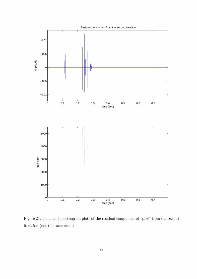
0 0.1 0.2 0.3 0.4 0.5 0.6 0.7

−0.01

−0.005

0

0.005

0.01

Residual component from the second iteration

ampl

itude

time (sec)

freq

(H

z)

time (sec)0 0.1 0.2 0.3 0.4 0.5 0.6 0.7

0

1000

2000

3000

4000

5000

Figure 21: Time and spectrogram plots of the residual component of “pike” from the second

iteration (not the same scale)

78

−0.6

−0.4

−0.2

0

0.2

0.4

0.6

ampl

itude

Original speech

−0.6

−0.4

−0.2

0

0.2

0.4

0.6

ampl

itude

Tonal component

0 0.2 0.4 0.6

−0.6

−0.4

−0.2

0

0.2

0.4

0.6

ampl

itude

Transient component

time (sec)

Original speech

freq

(H

z)

0

1000

2000

3000

4000

5000

Tonal component

freq

(H

z)

0

1000

2000

3000

4000

5000

Transient component

freq

(H

z)

time (sec)0 0.2 0.4 0.6

0

1000

2000

3000

4000

5000

Figure 22: Speech decomposition results of “pike”. Click to hear the sound of: original,

tonal, transient.

79

0 0.1 0.2 0.3 0.4 0.5−1

−0.8

−0.6

−0.4

−0.2

0

0.2

0.4

0.6am

plitu

de

Original speech

0 0.1 0.2 0.3 0.4 0.5−1

−0.8

−0.6

−0.4

−0.2

0

0.2

0.4

0.6

ampl

itude

Tonal component

0 0.1 0.2 0.3 0.4 0.5−1

−0.8

−0.6

−0.4

−0.2

0

0.2

0.4

0.6

ampl

itude

Transient component

time (sec)

Original speech

freq

(H

z)

0 0.1 0.2 0.3 0.4 0.50

1000

2000

3000

4000

5000

Tonal component

freq

(H

z)

0 0.1 0.2 0.3 0.4 0.50

1000

2000

3000

4000

5000

Transient component

freq

(H

z)

time (sec)0 0.1 0.2 0.3 0.4 0.5

0

1000

2000

3000

4000

5000

Figure 23: Speech decomposition results of “got”. Click to hear the sound of: original, tonal,

transient.

80

4.0 COMPARISONS OF TRANSIENT COMPONENTS AND CODING

RESULTS FROM VARIOUS ALGORITHMS

In this chapter, analysis of the transient components of 9 monosyllabic consonant-vowel-

consonant (CVC) words — bat, bot, boot, gat, got, goot, hat, hot, and hoot — is described.

These words were chosen because they represent relatively simple distinctions between tonal

and transient components. Constant formant frequency information in vowels is expected

to be included in the tonal component. Consonants, transitions from consonants to vowels,

transitions between vowels, and transitions at the end of vowels are expected to be included

in the transient component.

As stated earlier in Chapter 1, if our method captures statistical dependencies between

the MDCT coefficients and between the wavelet coefficients, it should provide more effective

identification of the transient components compared with an algorithm that ignores these

dependencies. To investigate this suggestion, the transient components identified by our

method and an implementation of Daudet and Torresani’s algorithm [12] are compared. The

transient components, identified by the algorithm of Yoo [77]1, are also analyzed. These

analyzes are described in Section 4.1.

In addition, if our method captures these statistical dependencies between coefficients,

it should provide more efficient coding results compared with the implementation of Daudet

and Torresani’s algorithm [12]. To test this suggestion, performance in terms of bit rate of

our method and the implementation of Daudet and Torresani’s algorithm [12], tested on 300

monosyllabic CVC words, are compared and results are discussed in Section 4.2. Implications

of this study are discussed in Section 4.3.

1The resulting transient components were received by personal communication with Sungyub Yoo.

81

Table 6: Nine CVC monosyllabic words

Set 1 Set 2 Set 3

Set 4 bat /bæt/ bot /bAt/ boot /bu:t/

Set 5 gat /gæt/ got /gAt/ goot /gu:t/

Set 6 hat /hæt/ hot /hAt/ hoot /hu:t/

4.1 TRANSIENT COMPARISONS

Nine monosyllabic CVC words terminated by a consonant /t/ were used in this study.

These words include bat (/bæt/), bot (/bAt/), boot (/bu:t/), gat (/gæt/), got (/gAt/),

goot (/gu:t/), hat (/hæt/), hot (/hAt/), and hoot (/hu:t/). These words allow us to investi-

gate six sets of words (three words each). More precisely, three sets of words differ in initial

consonants but have the same vowel (set 1 - set 3 columns in Table 6), and another three

sets of words have the same vowel but differ in initial consonants (set 4 - set 6 rows in Table

6). The sets are illustrated in Table 6. Spectrograms of these words are shown in Fig. 24.

Table 7 and Table 8 describe the components of the sets that we expect to be classified as

tonal and transient based on phonetic analysis.

4.1.1 Methods of Transient Comparisons

The transient components from our method were decomposed by the approach described in

Chapter 3. For the implementation of Daudet and Torresani’s algorithm [12], the numbers

of MDCT coefficients and the numbers of wavelet coefficients from our method were used

as the numbers of leading terms (significant coefficients) in their thresholding approach.

More precisely, in each iteration, the numbers of significant MDCT coefficients obtained

from the Viterbi algorithm were counted. Then the threshold was adjusted to yield the

same numbers of the MDCT coefficients in Daudet and Torresani’s algorithm [12], and the

tonal component was estimated by the inverse transform of those MDCT coefficients. The

82

bat

freq

(H

z)

0 0.2 0.40

2000

4000

bot

0 0.2 0.40

2000

4000

boot

0 0.2 0.40

2000

4000

gat

freq

(H

z)

0 0.2 0.40

2000

4000

got

0 0.2 0.40

2000

4000

goot

0 0.2 0.4 0.60

2000

4000

hat

time (sec)

freq

(H

z)

0 0.2 0.40

2000

4000

hot

time (sec)0 0.2 0.4

0

2000

4000

hoot

time (sec)0 0.1 0.2 0.3

0

2000

4000

Figure 24: Original speech. Click to hear the sound of: bat, bot, boot, gat, got, goot, hat,

hot, hoot.

83

Table 7: Original speech description

Consonant/ Appeared in Comments

Vowel

/b/ bat /bæt/ /b/, /g/, and /t/ has a clear time-frequency edge,

bot /bAt/ illustrated as a vertical ridge in the spectrogram.

boot /bu:t/ This information is expected to be included in the

/g/ gat /gæt/ transient components.

got /gAt/

goot /gu:t/

/t/ all words

/h/ hat /hæt/ /h/, which functions as a consonant, has a weak

hot /hAt/ period of noise with energy at the frequency level

hoot /hu:t/ of the formants of the following vowels [58]. This is

a good indicator that the algorithms can differentiate

the locally stationary part from the transient part

although they have the same formant patterns. This

information is expected to be included in the

transient components.

84

Table 8: Original speech description (continued)

Consonant/ Appeared in Comments

Vowel

/æ/ bat /bæt/ The vowels /æ/, /A/, and /u/ followed by /t/ were

gat /gæt/ investigated because these vowels have variations of

hat /hæt/ the second formant frequency in different directions.

/A/ bot /bAt/ More generally, the second formant frequency (F2)

got /gAt/ of /æ/ is fairly constant. On the other hand, F2 of

hot /hAt/ /A/ starts constant and then increases, while F2 of

/u/ boot /bu:t/ /u/ moves down. When these vowels follow a velar

goot /gu:t/ consonant /g/, there are noticeable transitions from

hoot /hu:t/ a coming together of the second formant and third

formant frequency [58]. These features allow us to

investigate how well the algorithms capture the

transitions in vowels.

85

numbers of significant wavelet coefficients obtained from the MAP algorithm were counted

and another threshold was adjusted to yield the same numbers of the wavelet coefficients

in Daudet and Torresani’s algorithm [12]. The transient component was estimated by the

inverse transform of those wavelet coefficients. Two iterations were used in our algorithm

and in the implementation of Daudet and Torresani’s algorithm [12].

By a personal communication with Sungyub Yoo, the transient components of these 9

words were obtained for comparison. They are referred to as the transient components from

the algorithm of Yoo [77].

4.1.2 Comparisons of Transient Components Identified by Various Algorithms

Figure 25, Fig. 26, and Fig. 27 illustrate tonal and transient components of the word “bat”

/bæt/ identified by our method, the implementation of Daudet and Torresani’s algorithm

[12], and the algorithm of Yoo [77], respectively. The word “bat” is composed of clear time-

frequency edges /b/ (A) and /t/ (B), illustrated as vertical ridges in the spectrogram, and

a vowel /æ/ has fairly constant frequency information in the first (F1), second (F2), third

(F3), and fourth formants (F4), illustrated as horizontal ridges in the spectrogram.

The tonal component identified by our method includes almost all of the constant fre-

quency information of the first (C), second (D), third (E), and fourth (F) formants and a

small part of the release of /t/ (G) illustrated as high intensity with constant frequency

information. These effective removals of constant frequency information in formants are

illustrated as holes in the transient component (J, K, and L). The transient component in-

cludes /b/ (H), /t/ (I), and transitions from /b/ to vowel /æ/, in between vowel /æ/, and

end of vowel /æ/. It also includes almost all of the release of /t/ illustrated as a noise pattern

emphasized in high frequency ranges (from 0.35 sec to end of the word).

The tonal component identified by the implementation of Daudet and Torresani’s algo-

rithm [12] includes almost all of constant frequency information of the first (C), second (D),

third (E), and fourth (F) formants but not as effectively as our method. Parts of constant

frequency information of the first, second, third, and fourth formants still left in the tran-

sient component shown as scattered intensity in the spectrogram. More information of the

86

release of /t/ (G) compared with our method was captured in the tonal component. Most of

clear time-frequency edges of /b/ (H) and /t/ (I) are included in the tonal component. The

transient component includes parts of /b/ (J), /t/ (K), and the release of /t/ (from 0.35 sec

to end of the word). It includes parts of transitions from /b/ to vowel /æ/, in between vowel

/æ/, and at the end of the vowel /æ/.

The tonal component identified by the algorithm of Yoo [77] includes most of constant

frequency information of the first (C) and second formants (D), and parts of constant fre-

quency information of the third (E) and fourth (F) formants. It also includes a small part of

the release of /t/ (G) similar to our method. The transient component includes /b/ (H), /t/

(I), and release of /t/. It also includes transitions from /b/ to vowel /æ/, in between vowel

/æ/, and end of vowel /æ/. However, the transient component includes parts of constant

frequency information of the second (J), most of constant frequency information of the third

(K) and fourth formants (L).

The tonal and transient components of 9 CVC words identified by our method are illus-

trated in Fig. 28 and Fig. 29 and summarized in Table 9, Table 10, and Table 11. From the

results, the constant frequency information in first, second, third, and fourth formants as

well as the slowly-varying frequency information are effectively included in the tonal com-

ponents. This can be seen as holes in the transient components. This approach is clearly

picking up edges in time-frequency expected to be transient information in the speech signal.

The tonal and transient components identified by the implementation of Daudet and

Torresani’s algorithm [12] are illustrated in Fig. 30 and Fig. 31 and summarized in Table

12 and 13. The transient components from this approach clearly show much more uniform

power throughout the words.

The tonal and transient components identified by the algorithm of Yoo [77] are illus-

trated in Fig. 32 and Fig. 33 and summarized in Table 14, Table 15, and Table 16. The

resulting transient components from this approach include time-frequency edges expected to

be transient information in speech. However, the transient components appear to include

significant constant frequency information of of higher formants.

87

bat

0

1000

2000

3000

4000

5000

Tonal component of "bat"

0

1000

2000

3000

4000

5000

Transient component of "bat"

freq

(H

z)

time (sec)0 0.05 0.1 0.15 0.2 0.25 0.3 0.35 0.4 0.45

0

1000

2000

3000

4000

5000

F1

F2

F3

F4

A B

H

C

D

E

F G

I

J

K

L

Figure 25: Original speech of the word “bat” (top), tonal (middle) and transient (bottom)

components identified by our method.

88

bat

0

1000

2000

3000

4000

5000

Tonal component of "bat"

0

1000

2000

3000

4000

5000

Transient component of "bat"

freq

(H

z)

time (sec)0 0.05 0.1 0.15 0.2 0.25 0.3 0.35 0.4 0.45

0

1000

2000

3000

4000

5000

F1

F2

F3

F4

A B

C

D

E

F G

K

H

J

I

Figure 26: Original speech of the word “bat” (top), tonal (middle) and transient (bottom)

components identified by the implementation of Daudet and Torresani’s algorithm [12].

89

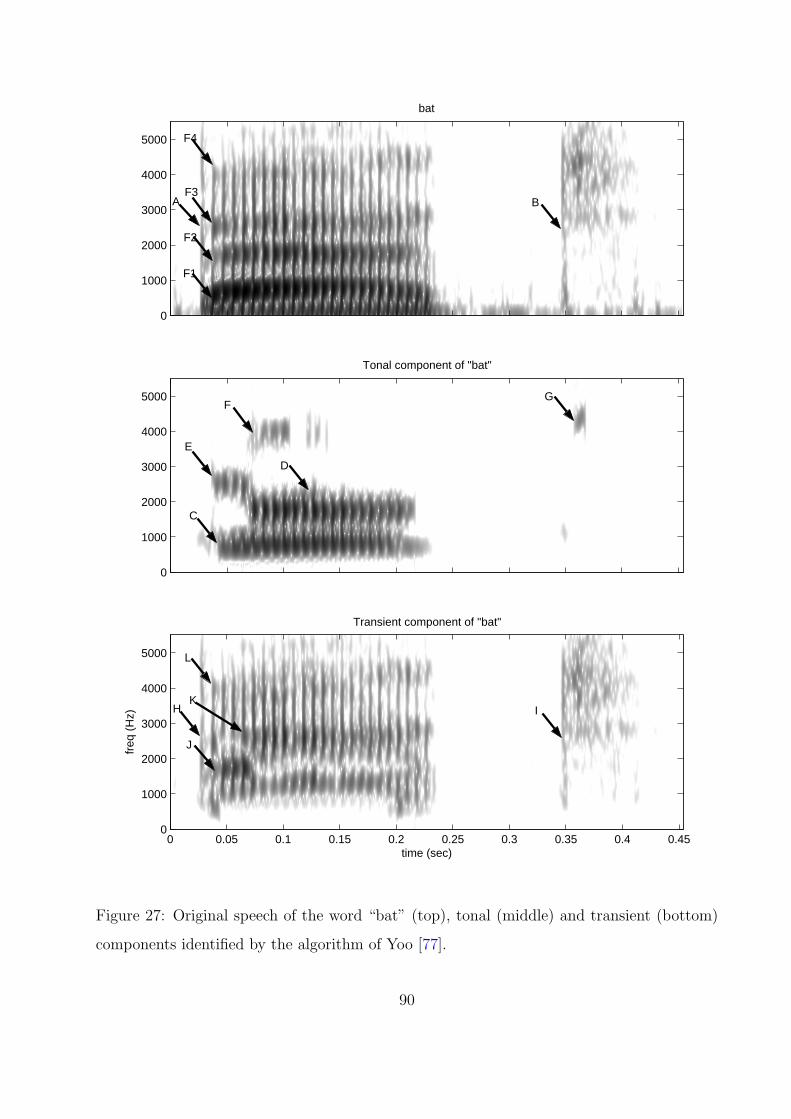
bat

0

1000

2000

3000

4000

5000

Tonal component of "bat"

0

1000

2000

3000

4000

5000

Transient component of "bat"

freq

(H

z)

time (sec)0 0.05 0.1 0.15 0.2 0.25 0.3 0.35 0.4 0.45

0

1000

2000

3000

4000

5000

F1

F2

F3

F4

A B

H

C

D

E

F G

I

J

K

L

Figure 27: Original speech of the word “bat” (top), tonal (middle) and transient (bottom)

components identified by the algorithm of Yoo [77].

90

Tonal component of "bat"

freq

(H

z)

0 0.2 0.40

2000

4000

Tonal component of "bot"

0 0.2 0.40

2000

4000

Tonal component of "boot"

0 0.2 0.40

2000

4000

Tonal component of "gat"

freq

(H

z)

0 0.2 0.40

2000

4000

Tonal component of "got"

0 0.2 0.40

2000

4000

Tonal component of "goot"

0 0.2 0.4 0.60

2000

4000

Tonal component of "hat"

time (sec)

freq

(H

z)

0 0.2 0.40

2000

4000

Tonal component of "hot"

time (sec)0 0.2 0.4

0

2000

4000

Tonal component of "hoot"

time (sec)0 0.1 0.2 0.3

0

2000

4000

Figure 28: Tonal components identified by our method. Click to hear the sound of: tonal of

“bat”, tonal of “bot”, tonal of “boot”, tonal of “gat”, tonal of “got”, tonal of “goot”, tonal

of “hat”, tonal of “hot”, tonal of “hoot”.

91

Transient component of "bat"

freq

(H

z)

0 0.2 0.40

2000

4000

Transient component of "bot"

0 0.2 0.40

2000

4000

Transient component of "boot"

0 0.2 0.40

2000

4000

Transient component of "gat"

freq

(H

z)

0 0.2 0.40

2000

4000

Transient component of "got"

0 0.2 0.40

2000

4000

Transient component of "goot"

0 0.2 0.4 0.60

2000

4000

Transient component of "hat"

time (sec)

freq

(H

z)

0 0.2 0.40

2000

4000

Transient component of "hot"

time (sec)0 0.2 0.4

0

2000

4000

Transient component of "hoot"

time (sec)0 0.1 0.2 0.3

0

2000

4000

Figure 29: Transient components identified by our method. Click to hear the sound of:

transient of “bat”, transient of “bot”, transient of “boot”, transient of “gat”, transient of

“got”, transient of “goot”, transient of “hat”, transient of “hot”, transient of “hoot”.

92

Table 9: Description of transient components identified by our method

Consonant/ Appeared in Comments

Vowel

/b/ bat /bæt/ clear time-frequency edges of /b/, /g/, and /t/

bot /bAt/ are included in the transient components. Most of

/g/ gat /gæt/ releases of /t/, illustrated as a noise pattern

got /gAt/ emphasized in high frequency ranges, are included in

goot /gu:t/ the transient components. Only parts of them,

/t/ all words appearing as high intensity with constant frequency

information, are included in tonal components. This

can be seen in the spectrograms of the tonal

components of “bat”, “gat”, “hat”, “got”, “boot”,

“goot”, and “hoot”.

/h/ hat /hæt/ Although /h/ has formants similar to the following

hot /hAt/ vowels, this information is included in the transient

hoot /hu:t/ components for “hot” and “hoot”. For the word “hat”,

parts of /h/ emphasized in second and third formants

and showed as constant frequency information are

included in the tonal component.

93

Table 10: Description of transient components identified by our method (continued)

Consonant/ Appeared in Comments

Vowel

/æ/ bat /bæt/ Vowel /æ/ in “bat” and “hat” has fairly constant

gat /gæt/ formant frequency information. The second formant

hat /hæt/ starts at a high frequency, then moves down and

remains constant in “gat”. The constant frequency

information of the first, second, third, and fourth

formants of these words is included in the tonal

components. For the word “gat”, slowly-varying

frequency information of the second formant is also

included in the tonal component. The transient

components include transitions from release of /b/,

/g/, and /h/ to the first, second, third, and fourth

formants of vowel /æ/ including transitions

at the end of /æ/.

94

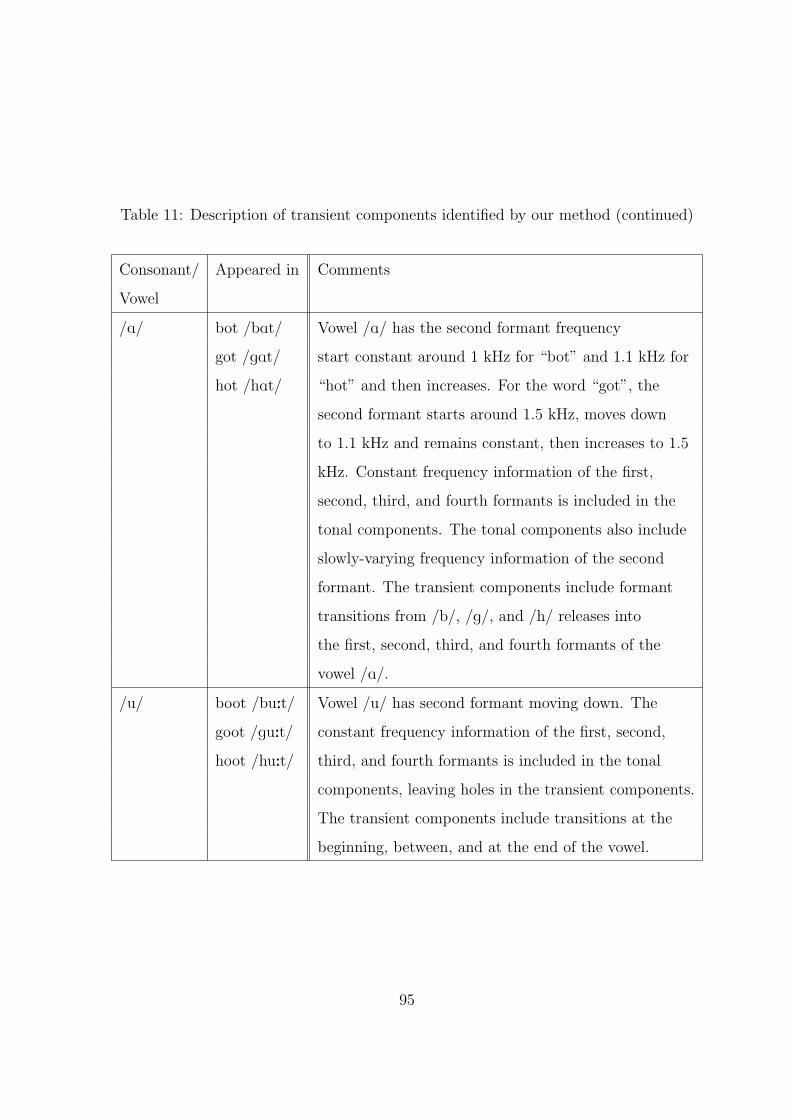
Table 11: Description of transient components identified by our method (continued)

Consonant/ Appeared in Comments

Vowel

/A/ bot /bAt/ Vowel /A/ has the second formant frequency

got /gAt/ start constant around 1 kHz for “bot” and 1.1 kHz for

hot /hAt/ “hot” and then increases. For the word “got”, the

second formant starts around 1.5 kHz, moves down

to 1.1 kHz and remains constant, then increases to 1.5

kHz. Constant frequency information of the first,

second, third, and fourth formants is included in the

tonal components. The tonal components also include

slowly-varying frequency information of the second

formant. The transient components include formant

transitions from /b/, /g/, and /h/ releases into

the first, second, third, and fourth formants of the

vowel /A/.

/u/ boot /bu:t/ Vowel /u/ has second formant moving down. The

goot /gu:t/ constant frequency information of the first, second,

hoot /hu:t/ third, and fourth formants is included in the tonal

components, leaving holes in the transient components.

The transient components include transitions at the

beginning, between, and at the end of the vowel.

95

Table 12: Description of transient components identified by Daudet and Torresani’s algo-

rithm [12].

Consonant/ Appeared in Comments

Vowel

/b/ bat /bæt/ Only parts of time-frequency edges of /b/ and /g/

bot /bAt/ are included in the transient components of “bat”,

boot /bu:t/ “gat”, “got”, and “goot”. These are clearly seen by

/g/ gat /gæt/ the lighter and discontinuous edges in spectrograms

got /gAt/ compared with more emphasized (darker) edges

goot /gu:t/ captured by our method. In addition, parts

/t/ all words of these edges are included in the tonal instead of the

transient components. Most of edges of /t/ in “bat”,

“boot”, “goot”, and “hoot” are included in the tonal

components and only parts of them are included in the

transient components. Clear time-frequency edges of

/t/ are included in “bot”, “hat”, and “hot”.

Most of releases of /t/ in “bat”, “boot”, “goot”,

and “hoot” are included in tonal instead of transient

components.

/h/ hat /hæt/ For the words “hat” and “hot”, parts of /h/ emphasized

hot /hAt/ in first, second, and third formants and showed as

hoot /hu:t/ constant frequency information are included in the

tonal components. For the word “hoot”, almost of /h/

is included in the transient component.

96

Table 13: Description of transient components identified by Daudet and Torresani’s algo-

rithm [12] (continued).

Consonant/ Appeared in Comments

Vowel

/æ/ bat /bæt/ Almost of the constant frequency information of the first,

gat /gæt/ second, third, and fourth formants in every word and

hat /hæt/ slowly-varying frequency information of the second

/A/ bot /bAt/ formant in “bot”, “boot”, “gat”, “got”, “goot”, “hot”,

got /gAt/ and “hoot” is included in the tonal components leaving

hot /hAt/ holes in the transient components. However, when looking

/u/ boot /bu:t/ at the spectrograms of the transient components, part of

goot /gu:t/ this information ia still left and spread over the vowels

hoot /hu:t/ compared with clean holes in the case of our

algorithm. In addition, transitions from consonants to

vowels, transitions in vowels, and transitions at the end

of vowels are not well emphasized as in the case of our

algorithm. These can be seen in the

spectrograms of every word compared with transitions

included in our method.

97

Tonal component of "bat"

freq

(H

z)

0 0.2 0.40

2000

4000

Tonal component of "bot"

0 0.2 0.40

2000

4000

Tonal component of "boot"

0 0.2 0.40

2000

4000

Tonal component of "gat"

freq

(H

z)

0 0.2 0.40

2000

4000

Tonal component of "got"

0 0.2 0.40

2000

4000

Tonal component of "goot"

0 0.2 0.4 0.60

2000

4000

Tonal component of "hat"

time (sec)

freq

(H

z)

0 0.2 0.40

2000

4000

Tonal component of "hot"

time (sec)0 0.2 0.4

0

2000

4000

Tonal component of "hoot"

time (sec)0 0.1 0.2 0.3

0

2000

4000

Figure 30: Tonal components identified by by the implementation of Daudet and Torresani’s

algorithm [12]. Click to hear the sound of: tonal of “bat”, tonal of “bot”, tonal of “boot”,

tonal of “gat”, tonal of “got”, tonal of “goot”, tonal of “hat”, tonal of “hot”, tonal of “hoot”.

98

Transient component of "bat"

freq

(H

z)

0 0.2 0.40

2000

4000

Transient component of "bot"

0 0.2 0.40

2000

4000

Transient component of "boot"

0 0.2 0.40

2000

4000

Transient component of "gat"

freq

(H

z)

0 0.2 0.40

2000

4000

Transient component of "got"

0 0.2 0.40

2000

4000

Transient component of "goot"

0 0.2 0.4 0.60

2000

4000

Transient component of "hat"

time (sec)

freq

(H

z)

0 0.2 0.40

2000

4000

Transient component of "hot"

time (sec)0 0.2 0.4

0

2000

4000

Transient component of "hoot"

time (sec)0 0.1 0.2 0.3

0

2000

4000

Figure 31: Transient components identified by the implementation of Daudet and Torresani’s

algorithm [12]. Click to hear the sound of: transient of “bat”, transient of “bot”, transient

of “boot”, transient of “gat”, transient of “got”, transient of “goot”, transient of “hat”,

transient of “hot”, transient of “hoot”.

99

Tonal component of "bat"

freq

(H

z)

0 0.2 0.40

2000

4000

Tonal component of "bot"

0 0.2 0.40

2000

4000

Tonal component of "boot"

0 0.2 0.40

2000

4000

Tonal component of "gat"

freq

(H

z)

0 0.2 0.40

2000

4000

Tonal component of "got"

0 0.2 0.40

2000

4000

Tonal component of "goot"

0 0.2 0.4 0.60

2000

4000

Tonal component of "hat"

time (sec)

freq

(H

z)

0 0.2 0.40

2000

4000

Tonal component of "hot"

time (sec)0 0.2 0.4

0

2000

4000

Tonal component of "hoot"

time (sec)0 0.1 0.2 0.3

0

2000

4000

Figure 32: Tonal components received by personal communication with Sungyub Yoo. Click

to hear the sound of: tonal of “bat”, tonal of “bot”, tonal of “boot”, tonal of “gat”, tonal

of “got”, tonal of “goot”, tonal of “hat”, tonal of “hot”, tonal of “hoot”.

100

Transient component of "bat"

freq

(H

z)

0 0.2 0.40

2000

4000

Transient component of "bot"

0 0.2 0.40

2000

4000

Transient component of "boot"

0 0.2 0.40

2000

4000

Transient component of "gat"

freq

(H

z)

0 0.2 0.40

2000

4000

Transient component of "got"

0 0.2 0.40

2000

4000

Transient component of "goot"

0 0.2 0.4 0.60

2000

4000

Transient component of "hat"

time (sec)

freq

(H

z)

0 0.2 0.40

2000

4000

Transient component of "hot"

time (sec)0 0.2 0.4

0

2000

4000

Transient component of "hoot"

time (sec)0 0.1 0.2 0.3

0

2000

4000

Figure 33: Transient components received by personal communication with Sungyub Yoo.

Click to hear the sound of: transient of “bat”, transient of “bot”, transient of “boot”,

transient of “gat”, transient of “got”, transient of “goot”, transient of “hat”, transient of

“hot”, transient of “hoot”.

101

Table 14: Description of transient components identified by the algorithm of Yoo [77].

Consonant/ Appeared in Comments

Vowel

/b/ bat /bæt/ Similar to the results from our method,

bot /bAt/ clear time-frequency edges of /b/, /g/, and /t/

/g/ gat /gæt/ are included in the transient components. No

got /gAt/ time-frequency edge is included in the tonal

goot /gu:t/ components. Most of releases of /t/ are included in

/t/ all words the transient components. Only parts of them are

included in the tonal components of “bat”, “”boot”,

and “hoot” as showed as high intensity in high

frequency of the spectrograms.

/h/ hat /hæt/ Almost all of /h/ is included in the transient

hot /hAt/ components. This can be seen as little information of

hoot /hu:t/ this consonant left in the tonal components showed in

the spectrograms.

102

Table 15: Description of transient components identified by the algorithm of Yoo [77] (con-

tinued).

Consonant/ Appeared in Comments

Vowel

/æ/ bat /bæt/ From the spectrograms of the tonal and transient

gat /gæt/ components, we can summarize as follow. For “bat”,

hat /hæt/ “gat”, and “hat”, almost of the constant frequency

information of the first formant, most of the constant

frequency information of the second formant, and small

part of the constant frequency information of the third

and fourth (for “bat”) formants is included in the tonal

components. The transient components of these words

include almost all of the constant frequency information

of the third and fourth formants, small part of the

constant frequency information of the second formant

(for “bat”), small part of the decreasing frequency

information of the second formant (for “gat”), and

include transitions from releases of consonants to vowel

103

Table 16: Description of transient components identified by the algorithm of Yoo [77] (con-

tinued).

Consonant/ Appeared in Comments

Vowel

/æ/, in vowel /æ/, and at the end of vowel /æ/.

/A/ bot /bAt/ The tonal components of these words include most of

got /gAt/ the constant frequency information of the first and

hot /hAt/ second formants, and most of constant frequency

information of the third formant for “bot”.

The transient components of these words include

constant frequency information of the third formant

for “got” and “hot” and fourth formant (for all

words), and significant tonal information of the

first and second formants. The transient components

include transitions from releases of consonants to

vowel /A/, in vowel, and at the end of vowel.

/u/ boot /bu:t/ Most of the constant frequency information of the second,

goot /gu:t/ third, and fourth formants of these words is included

hoot /hu:t/ in the tonal components. However, significant tonal

information in formants still appeared in the

transient components. Transitions from releases of

consonants to vowel /u/, in vowel, and at the end of

vowel are included in the transient components.

104

The energy of transient components identified by the three approaches is compared in

Table 17. Energy of the transient components identified by the algorithm of Yoo [77] have

very large energy on average (6.59%) followed by our method with medium energy on average

(0.74%), and the implementation of Daudet and Torresani’s algorithm [12] with smallest en-

ergy on average (0.23%). The average ratios of the energy of transient components identified

by three approaches are 29:3:1 (the algorithm of Yoo [77]:our method:the implementation of

Daudet and Torresani’s algorithm [12]).

4.2 SPEECH CODING COMPARISONS

Daudet and Torresani [12] proposed that decomposing a musical signal into tonal, transient,

and residual components and separately coding the individual components would produce

more efficient coding. Our interest is in isolating the transient component in speech itself,

but we investigated coding results as an indication of the improvement provided by our

version of the algorithm. If our method captures statistical dependencies, the significant

MDCT and wavelet coefficients should form clusters. With an encoding approach using the

run-length algorithm followed by Huffman coding, our method should provide more efficient

coding results compared to an algorithm that ignores the dependencies, i.e. the algorithm

of Daudet and Torresani [12]. To test this suggestion, coding performances in terms of bit

rate of the implementation of Daudet and Torresani’s algorithm [12] and our method were

compared.

105

Table 17: Energy of the transient components identified from various approaches.

Approach Transient energy of

bat bot boot

Our method 0.70% 0.73% 0.68%

The implementation of Daudet and Torresani’s algorithm [12] 0.18% 0.24% 0.22%

The algorithm of Yoo [77] 7.71% 3.44% 1.85%

Approach Transient energy of

gat got goot

Our method 0.88% 0.95% 0.59%

The implementation of Daudet and Torresani’s algorithm [12] 0.11% 0.17% 0.20%

The algorithm of Yoo [77] 16.14% 4.66% 1.56%

Approach Transient energy of

hat hot hoot

Our method 0.52% 0.78% 0.80%

The implementation of Daudet and Torresani’s algorithm [12] 0.22% 0.30% 0.39%

The algorithm of Yoo [77] 17.88% 5.50% 0.58%

106

4.2.1 Speech Coding Methods

Three-hundred monosyllabic CVC words were decomposed and encoded, and then the overall

bit rates (bits/sample) were compared. For a fair comparison, the same number of MDCT

coefficients from our method and from the implementation of Daudet and Torresani’s al-

gorithm [12] were used as described earlier in Section 4.1. Both approaches were run with

2 iterations i.e. the residual component from the first iteration was used in the role of the

original speech in the second iteration and the algorithm/method was repeated.

To compare the coding efficiency of our method to the implementation of Daudet and

Torresani’s algorithm [12], the significant MDCT and wavelet coefficients were quantized

using an 8-bit uniform quantizer. Based on an informal listening test, we found that an

8-bit uniform quantizer gave a reasonably low bit rate with a minimum perceived loss. The

quantized MDCT and wavelet coefficients were entropy encoded separately using a run-

length algorithm and Huffman coding (see [25], [33], [32] for review). We did not encode

the residual component for both approaches because we found that this component has very

small amplitude, and it includes very little information.

The average SNR of the decoded words reconstructed from quantized MDCT and wavelet

coefficients was computed, using the expression

SNR = 10 log10

{M−1∑n=0

s2(n)

M−1∑n=0

(s(n)− s(n))2

}, (4.1)

where s(n) is the original speech signal, and s(n) is the reconstructed speech signal.

4.2.2 Speech Coding Results

Table 18 shows the average bit rate used to encode the 300 test words. Our method re-

duced the bit rate compared with the implementation of Daudet and Torresani’s algorithm

[12] for each individual tested speech, with approximately the same sound quality based on

an informal listening test. Figure 34 shows one example of the reconstructed speech “lick”

/lIk/, which was encoded by our method and the implementation of Daudet and Torresani’s

107

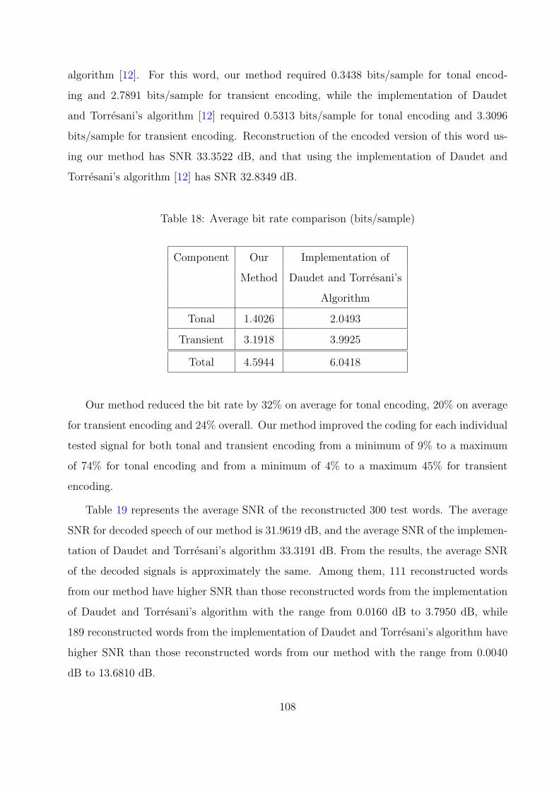
algorithm [12]. For this word, our method required 0.3438 bits/sample for tonal encod-

ing and 2.7891 bits/sample for transient encoding, while the implementation of Daudet

and Torresani’s algorithm [12] required 0.5313 bits/sample for tonal encoding and 3.3096

bits/sample for transient encoding. Reconstruction of the encoded version of this word us-

ing our method has SNR 33.3522 dB, and that using the implementation of Daudet and

Torresani’s algorithm [12] has SNR 32.8349 dB.

Table 18: Average bit rate comparison (bits/sample)

Component Our Implementation of

Method Daudet and Torresani’s

Algorithm

Tonal 1.4026 2.0493

Transient 3.1918 3.9925

Total 4.5944 6.0418

Our method reduced the bit rate by 32% on average for tonal encoding, 20% on average

for transient encoding and 24% overall. Our method improved the coding for each individual

tested signal for both tonal and transient encoding from a minimum of 9% to a maximum

of 74% for tonal encoding and from a minimum of 4% to a maximum 45% for transient

encoding.

Table 19 represents the average SNR of the reconstructed 300 test words. The average

SNR for decoded speech of our method is 31.9619 dB, and the average SNR of the implemen-

tation of Daudet and Torresani’s algorithm 33.3191 dB. From the results, the average SNR

of the decoded signals is approximately the same. Among them, 111 reconstructed words

from our method have higher SNR than those reconstructed words from the implementation

of Daudet and Torresani’s algorithm with the range from 0.0160 dB to 3.7950 dB, while

189 reconstructed words from the implementation of Daudet and Torresani’s algorithm have

higher SNR than those reconstructed words from our method with the range from 0.0040

dB to 13.6810 dB.

108

−0.2

−0.1

0

0.1

0.2

ampl

itude

(a)

−0.2

−0.1

0

0.1

0.2

ampl

itude

(b)

0 0.1 0.2 0.3 0.4

−0.2

−0.1

0

0.1

0.2

ampl

itude

(c)

time (sec)

(a)

freq

(H

z)

0

1000

2000

3000

4000

5000

(b)

freq

(H

z)

0

1000

2000

3000

4000

5000

(c)

freq

(H

z)

time (sec)0 0.1 0.2 0.3 0.4

0

1000

2000

3000

4000

5000

Figure 34: a) original speech “lick”, b) reconstruction of speech encoded by our method, and

c) reconstructed speech signal encoded by the implementation of Daudet and Torresani’s

algorithm [12]. Click to hear the sound of: original speech signal, decoded speech from our

method, decoded speech from the implementation of Daudet and Torresani’s algorithm [12].

109

Table 19: Average SNR comparison

Approach Our Implementation of

Method Daudet and Torresani

Algorithm

Average SNR 31.9619 33.3191

4.3 SUMMARY

The transient components identified by our method emphasize edges in time-frequency and

include transitions from the releases of the consonants into vowels, in between vowels, and at

the end of vowels compared with the transient components identified by the implementation

of Daudet and Torresani’s algorithm [12]. These differences appeared in spectrograms as

darker (higher energy) time-frequency edges and transitions. The transient components

identified by the algorithm of Yoo [77] retained a significant amount of energy during what

would appear to be tonal regions of speech, while our method removed this information more

effectively. These results suggest that our method can identify the transient information in

speech signal more effectively.

Our modified version of the algorithm of Daudet and Torresani [12] improved the cod-

ing efficiency for every tested signal, while providing approximately the same sound quality.

Although the resulting bit rates are too high to be useful for speech coding, we believe

that this improvement suggests that our method captures statistical dependencies between

the MDCT coefficients and between the wavelet coefficients and that capturing these de-

pendencies provides more effective separation of the tonal and transient components in the

speech.

110

5.0 SPEECH ENHANCEMENT AND PSYCHOACOUSTIC

EVALUATIONS

In the previous chapter, we showed that the transient component, identified by our method,

emphasizes edges in time-frequency and includes transitions from the releases of the conso-

nants into vowels, between vowels, and at the end of vowels. We believe that the transient

component may be particularly critical to speech perception and suggest that selective am-

plification of the transient component may improve speech perception in background noise.

To investigate this possibility, the transient component isolated by our method was selec-

tively amplified and recombined with the original speech to generate enhanced speech. The

energy of enhanced speech was adjusted to be equal to the energy of the original speech, and

the intelligibility of the original and enhanced speech was evaluated in eleven subjects using

the modified rhyme protocol described in Section 5.2. Psychoacoustic results and analysis

of confusions are described in this section. Implications of the results are summarized in

Section 5.3.

5.1 SPEECH ENHANCEMENT

Enhanced speech was generated by

xenha(t) = a(xorig(t) + b·xtran(t)), (5.1)

where xenha, xorig, and xtran represent the enhanced, original, and transient speech, respec-

tively. a is a factor to adjust the energy of the original and the enhanced speech to be equal

111

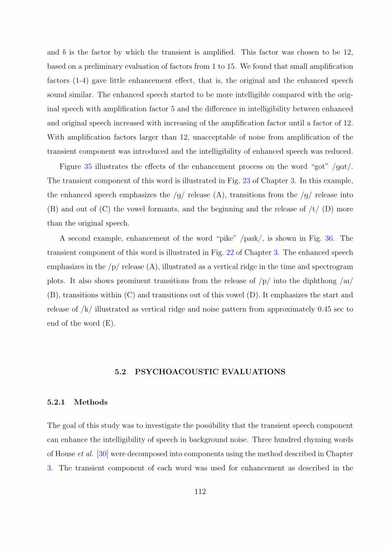
and b is the factor by which the transient is amplified. This factor was chosen to be 12,

based on a preliminary evaluation of factors from 1 to 15. We found that small amplification

factors (1-4) gave little enhancement effect, that is, the original and the enhanced speech

sound similar. The enhanced speech started to be more intelligible compared with the orig-

inal speech with amplification factor 5 and the difference in intelligibility between enhanced

and original speech increased with increasing of the amplification factor until a factor of 12.

With amplification factors larger than 12, unacceptable of noise from amplification of the

transient component was introduced and the intelligibility of enhanced speech was reduced.

Figure 35 illustrates the effects of the enhancement process on the word “got” /gAt/.

The transient component of this word is illustrated in Fig. 23 of Chapter 3. In this example,

the enhanced speech emphasizes the /g/ release (A), transitions from the /g/ release into

(B) and out of (C) the vowel formants, and the beginning and the release of /t/ (D) more

than the original speech.

A second example, enhancement of the word “pike” /paIk/, is shown in Fig. 36. The

transient component of this word is illustrated in Fig. 22 of Chapter 3. The enhanced speech

emphasizes in the /p/ release (A), illustrated as a vertical ridge in the time and spectrogram

plots. It also shows prominent transitions from the release of /p/ into the diphthong /aI/

(B), transitions within (C) and transitions out of this vowel (D). It emphasizes the start and

release of /k/ illustrated as vertical ridge and noise pattern from approximately 0.45 sec to

end of the word (E).

5.2 PSYCHOACOUSTIC EVALUATIONS

5.2.1 Methods

The goal of this study was to investigate the possibility that the transient speech component

can enhance the intelligibility of speech in background noise. Three hundred rhyming words

of House et al. [30] were decomposed into components using the method described in Chapter

3. The transient component of each word was used for enhancement as described in the

112

previous section. The modified rhyme protocol of Yoo [77], developed from House et al. [30]

and Mackersie and Levitt [40], was used to compare the intelligibility of enhanced speech to

original speech.

In the previous study of Yoo [77], eleven subjects suggested empirically to be a sufficient

sample to have statistical power. Therefore, eleven volunteer subjects with negative otologic

histories and having hearing sensitivity of 15 dB HL or better by conventional audiometry

(250 - 8 kHz) participated in this study. Fifty sets of rhyming monosyllabic CVC words

(6 words per set for a total of 300 words), were recorded by a male speaker [77]. Among

them, 25 sets differed in their initial consonants and 25 sets differed in their final consonants.

Subjects sat in the sound-attenuated booth and were asked to identify a target word from

a list of six words. The target word appeared on the computer screen and remained until

all of the six words were presented. These six words were presented at one of six SNR levels

(–25, –20, –15, –10, –5, and 0 dB) using speech-weighted background noise through the right

headphone. The subjects were asked to click the mouse as soon as they thought that they

heard the target word. The subjects could not change an answer and could not select a

previous word. The subjects were monitored during the test by skilled examiners under the

supervision of a certified clinical audiologist, and all subject responses were saved on the

computer.

The test procedure included a training session and the main test session. The training

session allowed the subjects to become familiar with the test. The training session included

12 trials — 6 trials of the original speech and 6 trials of the enhanced speech. The order

to perform the trial of original speech and the trial of enhanced speech was randomized.

The subjects heard the first 6 trials without background noise and the second 6 trials in

background noise. Each trial with background noise was randomly presented in one of 6

SNR levels and the same SNR level was not presented more than once.

The main session included 300 trials — 150 trials of the original speech and 150 trials

of the enhanced speech. The 150 trials of the original and enhanced speech were equally

distributed over the 6 SNR levels, giving 25 trials of original speech and 25 trials of enhanced

speech at each level of background noise. The target words were randomly chosen from the

300 rhyming words. Once a chosen target word was presented, it was removed from future

113

selections such that the same word did not occur as a target more than once. A short break

was provided to the subjects at the end of the first 100 trials and at the end of the second

100 trails.

5.2.2 Results

Statistical procedures specifically used to analyze the difference in the intelligibility for each

subject between two conditions, i.e. original and enhanced speech, are described as follows.

At each SNR level, the average percent correct responses for each subject for original and

enhanced speech were calculated as the subject’s correct responses divided by the total

number of stimuli as shown in Table 20 and Table 21.

At each SNR level, paired differences of each subject were calculated by using the average

percent correct responses of enhanced speech minus the average percent correct responses of

original speech as shown in Table 22. Means, standard deviations (SDs), and 95% confidence

intervals (CIs) (see [81] for review) of the paired-sample differences at each SNR level are

summarized in Table 23. The results suggest that there are substantial differences in speech

perception between the original and enhanced speech at –25dB, –20dB, and –15dB with

mean differences of 17.50%, 13.82%, and 7.64%, respectively. The CI of the differences in

intelligibility do not include zero at –25dB (p-value = 0.0012) and at –15dB (p-value =

0.0479).

To illustrate how the changes in absolute recognition rates vary with SNR level, figure 37

shows the percent correct responses averaged across subjects for original (dashed line) and

for enhanced speech (solid line) with group 95% CIs. The average percent correct responses

of the original and enhanced speech increased with increasing SNR levels, and the advantage

provided by enhancement decreases.

5.2.3 Analysis of Confusions

Confusions of consonantal elements in the initial and final positions were also analyzed. The

motivation for this analysis is to determine whether enhancement specifically affects some

sounds but not others. Because the 300 rhyming words are not phonetically balanced [30],

114

only the initial and final consonants with high frequency of occurrences, i.e. greater than

or equal to 20, were used in this analysis. Complete description responses of all subjects

and confusion matrices of consonantal elements in word-initial and word-final position are

summarized in Appendix C.

Figure 38 illustrates the average percent correct responses of consonantal elements in the

initial (11 consonants) and in the final positions (9 consonants) of original speech and of

enhanced speech at –25dB, –20dB, and –15dB. Each consonant was represented in terms of

coordinate (x,y), where x-value and y-value represent the average percent correct responses

across all subjects of original and enhanced speech, respectively. The average correct percent

correct responses were calculated by the numbers of correct responses divided by the total

number of responses (not the total number of stimuli as in Tables 20 and 21). This protocol

does not force subjects to make a response to every stimulus. In the case where the subjects

heard a target word and were not sure what they heard, they could either choose not to

respond or to guess. In this study, we would like to investigate confusions made by subjects

when they heard a particular sound but perceived a different sound. Therefore, we believe

that to exclude no responses from this study provides more effective analysis of confusions.

The dashed-line at 45◦ divides speech perception into 2 areas. Data points above the

45◦ line indicate consonantal elements that were recognized better in enhanced speech than

in original speech, and data points below this line indicate consonantal elements that were

recognized better in original speech than in enhanced speech.

Eight consonantal elements in initial and 10 consonantal elements in final positions were

recognized better in enhanced speech compared to original speech. These consonants are

summarized in Table 24. Only 1 consonantal element in initial position (/g/) and 1 conso-

nantal element in final position (/k/) were recognized less successfully in enhanced speech

than in original speech. These are both plosive stop consonants.

115

5.3 SUMMARY

The perception of the enhanced speech in noise is better than that of the original speech for

low SNR levels (–25, –20, and –15 dB). These results suggest that the transient component

is important in speech perception and emphasis of this component may provide an approach

to enhance intelligibility of the speech signal, especially in noisy environments.

The CI differences at –25dB and –15dB do not include zero, while CI difference at –20dB

includes zero. This occurred because of high variance (SD difference = 20.89) in the data,

specifically that of subject No. 5. At this SNR level, this subject perceived the original

speech (68%) much better than the enhanced speech (32%), resulting in a paired difference

equal to –36%.

The confusion analysis suggests that most consonants are consistently more intelligible in

enhanced speech. Only one consonantal element in initial position (/g/) and one consonantal

element in final position (/k/) were perceived less successfully in enhanced speech compared

to original speech. These two phonemes are velar plosive stop consonants, where /g/ is

voiced and /k/ is voiceless (see Appendix A for review). This finding supported the results

of Thomas [67] who used test materials of Egan [18] that were phonetically balanced test

materials and subjects were forced to answer to every stimulus. He found that most of the

confusions came from stop consonants [67].

In our study, the 300 rhyming words were not phonetically balanced [30] and the modified

rhyme protocol [77], based on a word-monitoring task [40], did not force the subjects to make

a response to every stimulus. More subjects would be required in order to analyze confusions

effectively. This analysis of confusions was presented as a preliminary study to evaluate the

use of confusion analysis to describe the effects of enhancement on different speech sounds.

116

0 0.05 0.1 0.15 0.2 0.25 0.3 0.35 0.4 0.45 0.5

−1

−0.5

0

0.5

(a) Original speech waveform

ampl

itude

0 0.05 0.1 0.15 0.2 0.25 0.3 0.35 0.4 0.45 0.5

−1

−0.5

0

0.5

(c) Enhanced speech waveform

ampl

itude

(b) Original speech spectrogram

freq

(H

z)

0 0.05 0.1 0.15 0.2 0.25 0.3 0.35 0.4 0.45 0.50

1000

2000

3000

4000

5000

(d) Enhanced speech spectrogram

freq

(H

z)

time (sec)0 0.05 0.1 0.15 0.2 0.25 0.3 0.35 0.4 0.45 0.5

0

1000

2000

3000

4000

5000

A

A

A

A

B

B

C

C

D

D

D

D

Figure 35: Original and enhanced version of “got”: (a) original speech waveform, (b) original

speech spectrogram, (c) enhanced speech waveform, and (d) enhanced speech spectrogram.

Click to hear the sound of: original, enhanced speech.

117

0 0.1 0.2 0.3 0.4 0.5 0.6 0.7−1

−0.5

0

0.5

(a) Original speech waveform

ampl

itude

0 0.1 0.2 0.3 0.4 0.5 0.6 0.7−1

−0.5

0

0.5

(c) Enhanced speech waveform

ampl

itude

(b) Original speech spectrogram

freq

(H

z)

0 0.1 0.2 0.3 0.4 0.5 0.6 0.70

1000

2000

3000

4000

5000

(d) Enhanced speech spectrogram

freq

(H

z)

time (sec)0 0.1 0.2 0.3 0.4 0.5 0.6 0.7

0

1000

2000

3000

4000

5000

A

A

A

A

B

B

C

C

D

D

E

E

E

E

B

B

Figure 36: Original and enhanced version of “pike”: (a) original speech waveform, (b) original

speech spectrogram, (c) enhanced speech waveform, and (d) enhanced speech spectrogram.

Click to hear the sound of: original, enhanced speech.

118

Table 20: Average percent correct responses of original speech

Subject No. Average percent correct responses (%)

–25 dB –20 dB –15 dB –10 dB –5 dB 0 dB

1 28 32 44 76 68 80

2 32 24 64 56 60 76

3 28 56 60 80 88 92

4 32 44 72 80 48 80

5 28 68 64 92 96 96

6 40 40 60 76 72 84

7 28 28 44 48 72 80

8 12 52 60 48 68 80

9 40 48 52 88 92 92

10 24 24 40 36 88 84

11 16 52 76 76 84 88

Mean 28.00 42.55 57.82 68.73 76 84.73

SD 8.58 14.34 11.64 18.49 14.86 6.40

119

Table 21: Average percent correct responses of enhanced speech

Subject No Average percent correct responses (%)

–25 dB –20 dB –15 dB –10 dB –5 dB 0 dB

1 64 64 60 76 80 72

2 24 56 60 64 76 100

3 56 52 64 72 76 84

4 40 56 68 76 68 88

5 44 32 80 76 88 68

6 56 68 80 80 88 80

7 48 56 64 64 68 92

8 48 72 56 72 64 72

9 60 68 60 68 72 72

10 32 48 60 68 68 84

11 28 48 68 80 80 92

Mean 45.45 56.36 65.45 72.36 75.27 82.18

SD 13.30 11.52 8.05 5.78 8.16 10.33

120

Table 22: Paired differences between enhanced and original speech

Subject No. Paired differences (%)

–25 dB –20 dB –15 dB –10 dB –5 dB 0 dB

1 36 32 16 0 12 –8

2 –8 32 –4 8 16 24

3 28 –4 4 –8 –12 –8

4 8 12 –4 –4 20 8

5 16 –36 16 –16 –8 –28

6 16 28 20 4 16 –4

7 20 28 20 16 –4 12

8 36 20 –4 24 –4 –8

9 20 20 8 –20 –20 –20

10 8 24 20 32 –20 0

11 12 –4 –8 4 –4 4

Table 23: Differences (enhanced speech – original speech) of means, standard deviations

(SDs), and 95% confidence intervals (CIs)

SNR Mean difference SD difference 95% CI difference

–25 dB 17.50 12.93 8.77 ∼ 26.14

–20 dB 13.82 20.89 –0.22 ∼ 27.85

–15 dB 7.64 11.24 0.09 ∼ 15.19

–10 dB 3.64 15.95 –7.08 ∼ 14.35

–5 dB –0.73 14.51 –10.48 ∼ 9.02

0 dB –2.55 14.56 –12.33 ∼ 7.24

121

−25 −20 −15 −10 −5 00

10

20

30

40

50

60

70

80

90

100

SNR

% c

orre

ct

Average percent correct responses between original and enhanced speech

Figure 37: Average percent correct responses between original (dashed line) and enhanced

speech (solid line)

122

0 10 20 30 40 50 60 70 80 90 1000

10

20

30

40

50

60

70

80

90

100

Average percent correct responses of consonantal elements of original vs enahanced speech at -25dB, -20dB, and -15dB

average percent correct responses of original speech

aver

age

perc

ent

corr

ect

resp

onse

s of

enh

ance

d sp

eech

initial positionfinal position

l

s

d

t

s

g

p f r

d

t

w

k

h m

k n g

b

p

Figure 38: Average percent correct responses according to phonetic elements in initial (♦)

and final (¤) positions between original and enhanced speech

123

Table 24: Consonantal elements in word-initial and word-final positions with high frequency

of occurrences (greater than or equal to 20)

phonetic category appeared in

initial position final position

voiceless plosive /p/, /t/, /k/ /p/, /t/, /k/

voiced plosive /b/, /d/, /g/ /d/, /g/

voiceless fricative /f/, /s/, /h/ /s/

nasal /m/, /n/

approximant /w/ /l/

alveolar trill /r/

124

6.0 MODIFIED VERSION OF ENHANCED SPEECH COMPONENTS

The objective of this evaluation is to examine how high-pass filtering of the enhanced com-

ponents affects the intelligibility of speech in background noise. The motivation of this

study is that the intelligibility of enhanced speech generated by the algorithm of Yoo [77]

is better than that of enhanced speech generated by our method. These two experiments

were performed at the Department of Communication Science and Disorders, University of

Pittsburgh using the same test protocol. Each experiment was performed in 11 subjects and

no subject participated in both experiments.

Results of these two experiments are compared in Fig. 39. At SNR levels of –20 dB,

–15 dB, and –10 dB, the differences in perceptions of original speech between these two

tests are negligible. However, at these SNR levels, the average percent correct responses of

the enhanced speech generated by our method are lower than those of the enhanced speech

generated by Yoo’s algorithm by about 10%.

The enhanced speech generated by Yoo’s algorithm [77] emphasized the high frequency

region because the transient component was identified from high-pass filtered speech. When

the amplitude of the enhanced speech was adjusted to be equal to that of the original speech,

the SNR in the high frequency region was effectively increased, which may have produced at

least some of the improvement seen by Yoo. The enhanced speech generated by our method

emphasized time-frequency edges over all frequency ranges, including the low-frequency re-

gion excluded by high-pass filtering in Yoo’s algorithm. Since part of the improvement seen

by Yoo’s enhanced speech may be due to high-pass filtering, we investigated the effect of

high-pass filtering on our version of enhanced speech. Our new version of enhanced speech

will be referred to as “modified version of enhanced speech.”

125

6.1 METHODS

Our modified version of enhanced speech was formed as follows. The transient component

identified by our method was high-pass filtered at 700 Hz (same filter as used in Yoo [77]).

Then, the high-pass filtered transient component was amplified by a factor of 18 and recom-

bined with the original speech. The energy of this enhanced speech version was adjusted to

be equal to that of the original speech in the same fashion as described in Chapter 5. The

factor of 18 was chosen to make the amount of transient energy added the same as before.

The average energy of the transient components of 300 rhyming words is higher than the

average energy of the transient components with high-pass filtering by a factor of 1.5, and

the amplification factor used to generate the enhanced speech as described in Chapter 5 was

12. Therefore, for the modified version of enhanced speech, the total multiplication factor

used to amplify the high-pass transient component was 18 (1.5× 12 = 18).

Another advantage of high-pass filtering of the transient component is that it removed

low frequency artifacts including pre-echo distortion as shown in the spectrogram (A) of

Fig. 40. These artifacts reduce the intelligibility of enhanced speech when the amplification

factor is larger than 12. Figure 40 shows two versions of the transient component of the

word “rip” /rIp/, spoken by a male speaker. The top plot illustrates the unfiltered transient

component amplified by a factor of 12, and the bottom plot illustrates the high-pass filtered

transient component amplified by a factor of 18.

Figure 41 shows time and spectrogram plots of the word “rip”, its enhanced version, and

the modified version of enhanced speech. From the figure, the enhanced speech emphasizes

time-frequency edges /r/ and /p/, and transitions of the second formant of the vowel /I/.

The modified version of enhanced speech emphasizes the time-frequency edge /r/ less than

the enhanced speech because of high-pass filtering, but it provides more emphases in the

higher frequency regions than the enhanced speech.

Five volunteer subjects with negative otologic histories and having hearing sensitivity of

15 dB HL or better by conventional audiometry (250 - 8 kHz) participated in this study.

The test was conducted in the same fashion as described in Chapter 5, except only one SNR

level (–20 dB) was used in this study and 200 trials were used instead of 300 trials.

126

The test procedure included a training session and the main test session similar to the

previous test. The main session included 100 trials of the enhanced speech and 100 trials of

the modified version of enhanced speech, which were presented randomly in speech-weighted

background noise. The target words were randomly chosen from the 300 rhyming words.

Once a chosen target word was presented, it was removed from future selections such that

the same word did not occur as a target more than once.

6.2 RESULTS

Table 25 presents average percent correct responses of each subject for the enhanced speech

and the modified version of enhanced speech. Paired differences for each subject were cal-

culated as the average percent correct responses of the modified version of enhanced speech

minus the average percent correct responses of enhanced speech. From the results, all sub-

jects perceived the modified version of enhanced speech better than the enhanced speech

with minimum improvement of 3% and maximum improvement of 11%.

Mean of the average percent correct responses for all subjects is 46% for enhanced speech

and 51.4% for the modified version of enhanced speech. The same statistical procedures

described in Chapter 5 were used to analyze whether there is significant difference in the

intelligibility between enhanced speech and modified version of enhanced speech. Statistics

of the paired-sample differences at –20 dB SNR level are: mean is 5.33%, standard deviation

(SDs) is 3.21%, and 95% confidence intervals (CIs) is 1.42% ∼ 9.38%. The results suggest

that there is significant difference in speech perception between the enhanced speech and

modified version of enhanced speech at –20 dB, since the CI of the difference in intelligibility

does not include zero (p-value = 0.0197).

127

6.3 DISCUSSION

For all subjects, at –20 dB, the perception of the modified version of enhanced speech in

background noise is significantly better than that of the enhanced speech. These results

suggest that emphasis of the high frequency region by high-pass filtering of the transient

component improves intelligibility of speech in background noise.

However, as shown in Fig. 42, the average percent correct responses of this experiment

(46%) is lower than those of the previous experiment at –20 dB (56%) by about 10%.

There are several factors that may contribute to the poorer performance of subjects in this

study than the previous study. First, this experiment was performed on a smaller number

of subjects (5 subjects) compared with the previous experiment (11 subjects), and most

of them (subject No. 1, 3, and 5) got much lower average percent correct responses on

our original version of enhanced speech than in the previous experiment. Second, different

protocols were used in these two experiments i.e. 300 trials equally randomized in 6 SNR

levels were used in the previous experiment, and 200 trials in the SNR level of –20 dB were

used in this experiment. Listening to trials at different levels of background noise might be

less challenging to subjects than listening to trials in one high level of background noise.

More precisely, when subjects heard a trial at low levels of background noise and recognized

a target word, they might be more able to do so at higher levels of background noise. On the

other hand, listening to target words in consistently high levels of background noise could

be frustrating to the subjects, resulting in poorer performance.

If we assume that the improvement in speech intelligibility provided by our modified

version of enhanced speech is consistent across subjects and experiments and if we apply

that improvement to the performance of the subjects in our first experiment, the averaged

percent correct responses of the modified version of enhanced speech would be expected to

be about 61% (56% + 5%), which is similar to, although lower than, Yoo’s result (70%).

The subjects in our first experiment had about 5% fewer correct responses at SNR levels

of 0 and –5 dB for both original speech and our original version of enhanced speech than

Yoo’s subjects, suggesting that our subjects overall may have been poorer performers in these

128

experiments. However, all of these differences are within the variability that we would ex-

pect between experiments, and we cannot conclude that there are any meaningful differences

between our modified version of enhanced speech and Yoo’s approach.

129

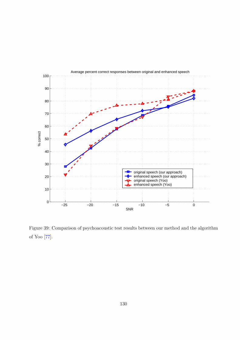
−25 −20 −15 −10 −5 00

10

20

30

40

50

60

70

80

90

100

SNR

% c

orre

ct

Average percent correct responses between original and enhanced speech

original speech (our approach)enhanced speech (our approach)original speech (Yoo)enhanced speech (Yoo)

Figure 39: Comparison of psychoacoustic test results between our method and the algorithm

of Yoo [77].

130

−0.6

−0.4

−0.2

0

0.2

0.4

0.6

0.8

ampl

itude

Transient amplified by 12

0 0.1 0.2 0.3 0.4

−0.6

−0.4

−0.2

0

0.2

0.4

0.6

0.8

ampl

itude

High−pass transient amplified by 18

time (sec)

Transient amplified by 12

freq

(H

z)0

1000

2000

3000

4000

5000

High−pass transient amplified by 18

time (sec)

freq

(H

z)

0 0.1 0.2 0.3 0.40

1000

2000

3000

4000

5000

A

Figure 40: Transient component amplified by 12 (top) and high-pass transient component

amplified by 18. Click to hear the sound of: transient multiplied by 12, high-pass transient

multiplied by 18.

131

−0.3

−0.2

−0.1

0

0.1

0.2

0.3

0.4

0.5

ampl

itude

Original speech

−0.3

−0.2

−0.1

0

0.1

0.2

0.3

0.4

0.5

ampl

itude

Enhanced speech

0 0.1 0.2 0.3 0.4

−0.3

−0.2

−0.1

0

0.1

0.2

0.3

0.4

0.5

ampl

itude

Modified version of enhanced speech

time (sec)

Original speech

freq

(H

z)

0

1000

2000

3000

4000

5000

Enhanced speech

freq

(H

z)

0

1000

2000

3000

4000

5000

Modified version of enhanced speech

freq

(H

z)

time (sec)0 0.1 0.2 0.3 0.4

0

1000

2000

3000

4000

5000

Figure 41: Original speech (top), enhanced speech (middle), modified version of enhanced

speech (botoom). Click to hear the sound of: original, enhanced speech, modified version of

enhanced speech. These three versions have the same energy.

132

Table 25: Average percent correct responses of enhanced speech and modified version of

enhanced speech

Subject No. Average percent correct responses (%)

Enhanced speech Modified version of Difference

enhanced speech

1 31 34 3

2 60 64 4

3 46 51 5

4 48 59 11

5 45 49 4

Mean 46 51.40 5.40

SD 10.32 11.46 3.21

133

−25 −20 −15 −10 −5 00

10

20

30

40

50

60

70

80

90

100

SNR

% c

orre

ct

Average percent correct responses between enhanced speech and modified enhanced speech

original speech (our approach)enhanced speech (our approach)original speech (Yoo)enhanced speech (Yoo)

Figure 42: Comparison of psychoacoustic test results between enhanced speech (•) and

modified enhanced speech (¥).

134

7.0 DISCUSSION AND FUTURE RESEARCH

7.1 DISCUSSION

We have introduced an alternative method to identify transient information in speech using

MDCT-based hidden Markov chain (HMC) and wavelet-based hidden Markov tree (HMT)

models. Our method, a modification of Daudet and Torresani [12], avoids thresholds and

describes the clustering and persistence statistical dependencies between the MDCT coeffi-

cients and between the wavelet coefficients. Persistence and clustering were represented by

two-state HMC and HMT models, using non-zero mean, mixtures of two univariate Gaus-

sian distributions. The initial parameters of the mixture were estimated by the greedy EM

algorithm [75]. By utilizing the Viterbi [57] and the MAP [17] algorithms to find the optimal

state distribution, the significant MDCT and wavelet coefficients were determined without

relying on a threshold [66].

A previous approach to identify the transient component in speech has been developed by

Yoo [77]. He employed three time-varying bandpass filters to remove the dominant formant

energies from speech. The original speech was high-pass filtered with 700 Hz cutoff frequency.

Three time-varying bandpass filters were manipulated to capture the strong formant energies

of the speech signal. The summation of these strong formant energies was considered to be

the tonal component. The tonal component was subtracted from the high-pass filtered

speech, resulting in the transient component.

Our method has advantages compared to the algorithm of Yoo [77]. First, our method

identifies the transient component of original speech without high-pass filtering and can

capture transient information in the low frequency range (0-700 Hz), which is not available

in the algorithm of Yoo [77]. Second, Yoo used bandpass filters that tracked specific formants

135

(only up to four formants), and his approach was less effective for higher formants. As a

result, the transient components identified by his approach retained a significant amount of

energy during what would appear to be tonal regions of speech, especially in high frequency

ranges. Our method appeared to remove this information more effectively. These differences

can be seen by comparing Fig. 33, that illustrates the transient components identified by

Yoo’s approach, to Fig. 29 that illustrates the transient components identified by our method.

The transient components identified by our method emphasize edges in time-frequency

and include transitions from the releases of the consonants into vowels, in between vowels,

and at the end of vowels to the greater extent than the transient components identified by

the implementation of Daudet and Torresani’s algorithm [12]. These results suggest that our

method identifies transient information in speech signal more effectively.

We believe that the more efficient coding results compared to the implementation of

Daudet and Torresani’s algorithm [12] suggests that our method captures statistical depen-

dencies between the MDCT coefficients and between the wavelet coefficients. We suggest that

capturing these dependencies provides more effective separation of the tonal and transient

components in speech. However, the coding results of our method are not efficient enough

to be useful in speech coding. Our goal was to identify tonal and transient components

effectively, and we were not concerned with bit rate.

One reason for the high bit rates is that a short half-window length (2.9 ms) was used

in MDCT, while a much longer half-window length (23.22 ms) was used by Daudet and

Torresani [12]. The short window length minimized pre-echo distortion, but the coding

gain was reduced. However, the pre-echo distortion in MDCT is not completely removed

and that effect is still observed in the transient component. This effect is more prominent

with amplification of the transient component when generating the enhanced speech and

may explain why our enhanced speech became less intelligibility when the multiplication

factor was increased above 12. The pre-echo distortion may contribute to degradation of the

intelligibility of the enhanced speech at lower SNRs compared to the scores obtained by Yoo

[77], as shown in Fig. 42.

Another reason for lower intelligibility scores of the enhanced speech generated by our

method compared to the algorithm of Yoo [77] is that the transient component identified

136

by Yoo’s approach emphasized the high frequency region. Yoo’s improvement probably

includes an effect of high-pass filtering known to improve speech intelligibility in background

noise [50]. However, our method includes low frequency energy in the transient component

and does not benefit from that boost. We suggest that about 7% (the average percent

improvement of enhanced speech over original speech in our experiments at all SNR levels)

of improvement of speech perception in background noise in both Yoo’s and our experiments

may be due to transient enhancement rather than high-frequency emphasis.

Our second experiment with the modified enhanced speech suggests that combining high-

pass filtering with speech enhancement using our transient speech component increases the

improvement in speech intelligibility by about 5%. The variability inherent to psycho-

acoustic experiments complicated our attempts to compare our results in the two experi-

ments and to compare them to Yoo’s results, as discussed in Section 6.3, even though the

experimental protocols were very similar. The intelligibility scores on our original version

of enhanced speech for the subjects in our second experiment were lower than the scores

on the same stimuli for the subjects in our first experiment, even though pilot tests with

experienced subjects did not show this difference. In addition, the subjects in our two groups

appeared to have different overall levels of performance and may have had poorer overall

performance than Yoo’s subjects. It is possible that a difference in the level of experience of

the different groups of subjects affected the results. The percent correct responses obtained

with our modified version of enhanced speech appear to be lower than results obtained by

Yoo, but, because of experimental variability, we do not conclude that there are meaningful

differences between the two approaches.

The specific contributions that have been made in this project are listed below:

• Introduced a method to identify a transient component in speech signal. Our method has

been developed from the approaches of Daudet and Torresani [12], Molla and Torresani

[48], and Daudet et al. [10], where these approaches were intended to achieve a low bit

rate with minimum perceived loss in encoding a musical signal. These researchers did

not identify the transient component in speech.

137

• Applied the hidden Markov chain (HMC) model and the hidden Markov tree (HMT)

model to capture statistical dependencies, assumed to be independent in Daudet and

Torresani [12], between the MDCT coefficients and between the wavelet coefficients,

respectively.

• Applied the Viterbi and the MAP algorithms to find the optimal state distribution of

the MDCT and the wavelet coefficients that resulted in determinations of the significant

MDCT and wavelet coefficients without relying on threshold as did Daudet and Torresani

[12].

• Modeled the MDCT and the wavelet coefficients as a non-zero mean Gaussian mixture

instead of a zero mean Gaussian mixture as did Daudet et al. [10] and Molla and

Torresani [48]. The non-zero mean model allowed better fit of the model to the data. We

believe that this better fit provides more effective identification of the tonal and transient

components.

• Applied the greedy EM algorithm [75], suggested to be less sensitive to initial parameter

initialization than the EM algorithm [13], to estimate initial parameters (means and

variances) of the HMC and HMT modeled as a mixture of two univariate Gaussian

distributions. We believe that with better initializations of the models, more effective

estimations of the tonal and transient components can be obtained.

• Showed experimentally that 3 mixture components and then the MoM as suggested by

Scott and Szewczyk [60] does not have an advantage over 2 mixture components when

fitting a mixture of two univariate Gaussian distributions with means not well separated

using the greedy EM algorithm.

• Evaluated the speech enhancement approach based on time-frequency analysis with a

formal psychoacoustic experiment and analysis of confusions of consonants both in initial

and final positions.

138

7.2 FUTURE RESEARCH

• Several approaches have been proposed to reduce pre-echo distortion, such as bit reser-

voirs, window switching, gain modification, switched filter banks, and temporal noise

shaping [52]. A better understanding of the pre-echo effect distortion may suggest im-

provements in the tonal estimation that will provide better identification of the transient

component in speech signal.

• The Daubechies-8 was used as a mother wavelet in transient estimation. The use of

other mother wavelets including wavelet packet may provide better identification of the

transient component in speech signal.

• The transient component high-pass filtered at 700 Hz was used to generate the modified

version of enhanced speech. We suggest that the high-pass filtered version of transient

component can be generated equivalently using the wavelet transform, as follow. Let the

sampling frequency of the speech signal be Fs Hz, then T = 1/Fs. At scale level j, the

coefficients sampling period will be jT and the frequency will be 1/jT = Fs/j. Therefore,

if only those decomposition levels i.e. j > Fs/700 are considered, the resulting transient

component will be equivalent to the high-pass filtered version at 700 Hz.

• Although our method has been developed to enhance the intelligibility of speech be-

fore it is degraded by noise, we suggest that our approach may be used to enhance the

intelligibility of speech already degraded by noise e.g. white noise. The residual com-

ponent is expected to have a flat spectrum. Therefore, it should predominantly include

the background noise. The transient component can be used further to enhance the

intelligibility of denoised speech signal (tonal + transient), and that may provide an-

other speech enhancement approach that can be used in lower SNR levels compared with

previous studies [16], [37], [55], [70].

• The psychoacoustic test protocol [77] used in this project was developed from the use

of 300 rhyming words (monosyllabic CVC words) [30] and idea of closed-set monitoring

task [40] suggested to reduce inflated scores by allowing subjects not to answer to every

stimulus. However, the stimulus is a monosyllabic CVC word. In order to make a correct

response, the subjects could possibly focus only on the first or the last phoneme, especially

139

when the target word appearing on the computer screen was not presented in the first

order. As a result, they would know that a group of trials differ in the initial or final

position. We suggest that different types of stimuli such as sentences with various types

of noises and possibly spoken by different speakers may be another approach to evaluate

speech intelligibility in noise more effectively. This may result in a better understanding

of the transient component in speech, including quantitative measures and definitions

that may suggest other approaches that are more effective to identify it.

140

APPENDIX A

THE BASIC SOUND OF ENGLISH

In this Appendix, the basic consonants and vowels of General American (GA) English, which

is spoken in the central and western areas of America [58], are described. This Appendix

is intended for readers, who are not familiar with vowels and consonants especially in the

phonetic forms as referred to throughout this dissertation.

Consonants are reviewed—based on voicing, place of articulation, and manner of articulation—

as summarized in Table 26. Vowels are reviewed, based on the shape and the position of the

tongue in the month and the shape of the lips. Summaries of vowels are illustrated in Fig. 43.

In addition, glides and diphthongs are reviewed. Transcription, the phonetic symbols used

to express how a word is pronounced [58], and symbols used in this dissertation, follow the

usage recommended by the International Phonetic Association [31]. This system, known as

the International Phonetic Alphabet, is the most widely used set of symbols [58]. Both the

Association and the Alphabet are known as the IPA [31]. All examples illustrated in this

Chapter were chosen from Oxford Advanced Learner’s Dictionary [27].

A.1 CONSONANTS

Rogers defined consonants as “sounds that involve a major obstruction or constriction of

the vocal tract” [58]. Consonants can be classified along three dimensions—voicing, place

of articulation, and manner of articulation [58]. In terms of voicing, consonants can be

141

categorized into voiceless and voiced. Voiceless sounds are made with the vocal folds apart

[58] such as /p/ in pan and /t/ in tan. Voiced sounds, on the other hand, are made with

the vocal folds close together [58] such as /b/ in big and /d/ in dig. The place where the

obstruction of the consonant is made is described as the place of articulation; the nature

of obstruction is described by the manner of articulation [58]. Description in this section

follows Rogers [58] and the IPA Handbook [31].

A.1.1 Place of Articulation

A.1.1.1 Bilabial In English, the bilabial consonants, produced by completely closing

of lips and the articulation of the upper lip against the lower lip, are composed of /p b m/

as in the initial sounds of the words pan, ban, man. The sound /p/ is voiceless and /b m/

are voiced.

/p/ par, sleepy, map

/b/ back, shabby, sub

/m/ man, hammer, ram

A.1.1.2 Labiodental The sounds produced by the articulation of the lower lip against

the upper teeth are called labiodental. Labiodental sounds in English are composed of /f v/,

as in the initial sounds of the words fan and van. /f/ is voiceless and /v/ is voiced [31].

/f/ fan, differ, graph

/v/ van, moving, glove

A.1.1.3 Dental There are two dental sounds in English. These sounds normally are

written with the letters th. The initial sound of thank is voiceless /T/, and the initial sound

of that is voiced /D/.

/T/ (called theta) thank, athlete, wealth

/D/ (called eth) that, neither, teeth

142

A.1.1.4 Alveolar The sounds produced by the tip of tongue hitting the alveolar ridge

are called alveolar consonants. These sounds are composed of /t d s z n l/, where /t s/ are

voiceless, and /d z n l/ are voiced.

/t/ tap, retard, kissed

/d/ do, middle, moved

/s/ seed, loser, loss

/z/ zip, lazy, tease

/n/ now, many, sun

/l/ loan, rely, bull

A.1.1.5 Postalveolar The area between the rear of the alveolar ridge and the border

of the palate is referred as the postalveolar area. Four sounds in English /S Z tS dZ/ are

made in this area. /S/, usually written with the letters sh, is voiceless as the initial sound

in the word shade. The voiced version of this sound, /Z/, is found as in the middle of the

word pleasure. The initial sound in the word check, transcribed /tS/, and the initial sound

in gene, transcribed /dZ/, are other two sounds in the postalveolar. /tS/ is voiceless, and

/dZ/ is voiced.

/S/ (called esh) shape, ashamed, english

/Z/ (called ezh) measure, television

/tS/ chain, teacher, rich

/dZ/ jean, virology, visage

A.1.1.6 Retroflex The sound produced by the tip of tongue approaching (but not

actually touching) the back of the alveolar ridge is called retroflex /ô/, as the initial sound

in real.

/ô/ read, marry

143

A.1.1.7 Palatal The sound produced by articulation of the front of the tongue against

the palate is called palatal. In English, only /j/, as the initial sound in yes, is palatal.

/j/ (called yod) yoke, opinion excuse

A.1.1.8 Velar Velar is produced by the back of the tongue articulating against the

velum. In English the velars are /k g N/.

/k/ key, maker, lock

/g/ get, baggage, bag

/N/ linger, sing

A.1.1.9 Labial-velar A sound that has a double place of articulation, both labial and

velar, is called labial-velar, such as the sound /w/.

/w/ wash, way

In addition, General American (GA) English has a voiceless labial-velar sound /û/.

/û/ what, where

A.1.2 Manner of Articulation

Rogers defined the manner of articulation as “the degree and kind of constriction in the vocal

tract” [58]. He explained manners of articulation in making /t/ and /s/ sounds. In making

/t/, the tongue is raised to the alveolar ridge, sealing the vocal tract so that no air passing

out. On the other hand, making /s/, there is a gap between the articulators. Therefore air

can pass out. He mentioned that a long /tttttt/ cannot be made but a long and continuous

/ssssss/ can be made.

A.1.2.1 Stops A complete closure, resulting in no air passing out of the mouth, is called

a stop. In English, six consonants, /p t k b d g/, are stops. In addition, the nasal stops /m

n N/ can be considered as a special kind of stop.

144

A.1.2.2 Fricatives Sounds made by a small opening allowing air to escape with some

friction resulting in friction-like noise are called fricatives. The fricatives in English are /f v

T D s z S Z û/.

A.1.2.3 Approximants Approximants, absent of frication, are consonants with a greater

opening in the vocal tract than fricatives. In English, all approximants are voiced, composed

of /l ô w j/.

A.1.2.4 Affricates In English, the affricates, sequences of stops and fricatives, are /tS

dZ/.

A.1.2.5 Nasals In English, the sounds /m n N/ are called nasals or nasal stops. In

making these sounds, the velum is lowered and the air is passed out through the nose.

A.1.3 Summary of GA English Consonants

Table 26 summarizes GA English consonants. Symbols appear in pairs, the left symbol

represents voiceless and the right symbol represents voiced consonants, respectively.

A.2 VOWELS

A.2.1 How Vowels Are Made

Rogers [58] stated that in making vowels, the vocal tract is more open than it is when making

consonants. The shape and the position of the tongue in the mouth and the shape of the lips

are primarily involved [58]. He mentioned that when making the vowel in the word he, the

front of the tongue is close to the forward part of the palate and this vowel is considered to be

a high front vowel, transcribed as /i/. When making the vowel in ah, the tongue moves back

and is lowered. He stated that this vowel is considered to be a low back vowel, transcribed

as /A/. Again, description in this section follows Rogers [58] and the IPA Handbook [31].

145

Table 26: GA English consonants [58]

bilabial labiodental dental alveolar postalveolar

stop p b t d

fricative f v T D s z S Z

affricate tS dZ

nasal m n

approximant l

retroflex palatal velar labial-velar

stop k g

fricative û

affricate

nasal N

approximant ô j w

The primary factor in determining the quality of a vowel is the shape of the tongue,

and phoneticians have often described vowels by the location of the highest point of the

tongue. Other vowels in GA English have different highest points of the tongue and can be

represented by the chart in Figure 43.

A.2.1.1 Glides Glides are vowels moving rapidly from one vowel position to another.

Rogers mentioned that glides are phonetically similar to vowels but their functions are con-

sidered as either consonants before a vowel or as a syllable nucleus after a vowel.

Rogers described the shape and the position of the tongue in the mouth and the shape

of the lips in making two glides in English, /j/ and /w/, as

The glide /j/ moves to or from a high front unrounded position. In the word like

yell /jEl/, the tongue starts at a high front unrounded position — approximately

146

the position for /i/ — and then moves to the lower /E/ position. The glide /w/ is

similar, except that it moves either to or from a high, back rounded position; a word

like well, starts at a high, back rounded position — like the position for /u/ — and

moves to an /E/ position [58].

/j/ yard, yacht, yen

/w/ warm, wing, web

A.2.1.2 Diphthongs A diphthong can be defined as a sequence of a simple vowel and

a glide.

Rogers described a diphthong in the word cow. Disregarding the /k/, there are two

parts to the rest of this word, where this diphthong starts from a low vowel and then moves

upwards to a vowel sound like /u/. The first portion of this diphthong is /a/ and the second

portion moves and is a glide /w/. Further, he mentioned that the diphthongs /aw aj Oj/ all

start with low vowel and have long glides, either to a high front or high back position.

/aj/ lie, high, writhe, eye

/aw/ how, count, ounce, rebound

/Oj/ boy, moist, deploy, oil

Rogers mentioned that the diphthongs /ej ow/ start from a mid vowel with glides shorter

than the low diphthongs.

/ej/ may, jade, sail

/ow/ so, coat, vote

A.2.1.3 The GA Vowel System The GA vowel system is summarized below.

GA has the following vowels:

i u

I U

ej @ ow

E 2 O Oj

æ A aj aw

147

bead i root u

sit I pull U

jade ej about @ how ow

yell E mud 2 saw O joy Oj

cat æ calm A five aj now aw

Figure 43 illustrates different simple vowels adapted from the IPA chart [31], where

position in the chart represents the position of the tongue in the mouth.

i

E

A

Q

U

u

√ ç

I

´

Front Central BackClose

Close-mid

Open-mid

Open

Figure 43: GA vowel chart adapted from the IPA chart [31]: symbols appear in pairs, the

left symbol represents an unrounded vowel and the right symbol represents a rounded vowel.

148

APPENDIX B

THREE HUNDRED RHYMING WORDS

This appendix lists the 300 rhyming words [30] used in the psychoacoustic test, where 150

words differ in initial consonants (Table 27) and another 150 words differ in final consonants

(Table 28). These lists were ordered alphabetically.

149

Table 27: Lists of 150 rhyming words (various consonantal elements in initial position)

Ensemble No. Stimulus words

I1 red /rEd/ wed /wEd/ shed /SEd/ bed /bEd/ led /lEd/ fed /fEd/

I2 sold /sold/ told /told/ hold /hold/ cold /cold/ gold /gold/ fold /fold/

I3 fig /fIg/ pig /pIg/ rig /rIg/ dig /dIg/ wig /wIg/ big /bIg/

I4 lick /lIk/ pick /pIk/ tick /tIk/ wick /wIk/ sick /sIk/ kick /kIk/

I5 look /lUk/ hook /hUk/ cook /kUk/ book /bUk/ took /tUk/ shook /SUk/

I6 dark /dark/ lark /lark/ bark /bark/ park /park/ mark /mark/ hark /hark/

I7 tale /tel/ pale /pel/ male /mel/ bale /bel/ gale /gel/ sale /sel/

I8 feel /fil/ eel /il/ reel /ril/ heel /hil/ peel /pil/ keel /kil/

I9 hill /hIl/ till /tIl/ bill /bIl/ fill /fIl/ kill /kIl/ will /wIl/

I10 oil /OIl/ foil /fOIl/ toil /tOIl/ boil /bOIl/ soil /sOIl/ coil /cOIl/

I11 game /gem/ tame /tem/ name /nem/ fame /fem/ same /sem/ came /kem/

I12 men /men/ then /Den/ hen /hen/ ten /ten/ pen /pen/ den /den/

I13 din /dIn/ tin /tIn/ pin /pIn/ sin /sIn/ win /wIn/ fin /fIn/

I14 gun /g2n/ run /r2n/ nun /n2n/ fun /f2n/ sun /s2n/ bun /b2n/

I15 bang /bæN/ rang /ræN/ sang /sæN/ gang /gæN/ hang /hæN/ fang /fæN/

I16 tent /tEnt/ bent /bEnt/ went /wEnt/ sent /sEnt/ rent /rEnt/ dent /dEnt/

I17 tip /tIp/ lip /lIp/ rip /rIp/ dip /dIp/ sip /sIp/ hip /hIp/

I18 cop /kap/ top /tap/ mop /map/ pop /pap/ shop /Sap/ hop /hap/

I19 seat /sit/ meat /mit/ beat /bit/ heat /hit/ neat /nit/ feat /fit/

I20 wit /wIt/ fit /fIt/ kit /kIt/ bit /bIt/ sit /sIt/ hit /hIt/

I21 hot /hat/ got /gat/ not /nat/ tot /tat/ lot /lat/ pot /pat/

I22 rest /rEst/ best /bEst/ test /tEst/ nest /nEst/ vest /vEst/ west /wEst/

I23 rust /r2st/ dust /d2st/ just /dZ2st/ must /m2st/ bust /b2st/ gust /g2st/

I24 raw /rO/ paw /pO/ law /lO/ saw /sO/ thaw /TO/ jaw /dZO/

I25 day /de/ say /se/ way /we/ may /me/ gay /ge/ pay /pe/

150

Table 28: Lists of 150 rhyming words (various consonantal elements in final position)

Ensemble No. Stimulus words

F1 bat /bæt/ bad /bæd/ back /bæk/ bath /bæT/ ban /bæn/ bass /bæs/

F2 bead /bid/ beat /bit/ bean /bin/ beach /biÙ/ beam /bim/ beak /bik/

F3 buck /b2k/ but /b2t/ bun /b2n/ bus /b2s/ buff /b2f/ bug /b2g/

F4 cave /kev/ cane /ken/ came /kem/ cape /kep/ cake /kek/ case /kes/

F5 cut /c2t/ cub /c2b/ cuff /c2f/ cuss /c2s/ cud /c2d/ cup /c2p/

F6 dim /dIm/ dig /dIg/ dill /dIl/ did /dId/ din /dIn/ dip /dIp/

F7 dud /d2d/ dub /d2b/ dun /d2n/ dug /d2g/ dung /d2N/ duck /d2k/

F8 fin /fIn/ fit /fIt/ fig /fIg/ fizz /fIz/ fill /fIl/ fib /fIb/

F9 heap /hip/ heat /hit/ heave /hiv/ hear /hir/ heath /hiT/ heal /hil/

F10 king /kIN/ kit /kIt/ kill /kIl/ kin /kIn/ kid /kId/ kick /kIk/

F11 lake /lek/ lace /les/ lame /lem/ lane /len/ lay /le/ late /let/

F12 mat /mæt/ man /mæn/ mad /mæd/ mass /mæs/ math /mæT/ map /mæp/

F13 pane /pen/ pay /pe/ pave /pev/ pale /pel/ pace /pes/ page /pedZ/

F14 pan /pæn/ path /pæT/ pad /pæd/ pass /pæs/ pat /pæt/ pack /pæk/

F15 peat /pit/ peak /pik/ peace /pis/ peas /piz/ peal /pil/ peach /piÙ/

F16 pip /pIp/ pit /pIt/ pick /pIk/ pig /pIg/ pill /pIl/ pin /pIn/

F17 pus /p2s/ pup /p2p/ pun /p2n/ puff /p2f/ puck /p2k/ pub /p2b/

F18 rate /ret/ rave /rev/ raze /rez/ race /res/ ray /re/ rake /rek/

F19 sake /sek/ sale /sel/ save /sev/ same /sem/ safe /sef/ sane /sen/

F20 sad /sæd/ sass /sæs/ sag /sæg/ sat /sæt/ sap /sæp/ sack /sæk/

F21 seem /sim/ seethe /siD/ seep /sip/ seen /sin/ seed /sid/ seek /sik/

F22 sip /sIp/ sing /sIN/ sick /sIk/ sin /sIn/ sill /sIl/ sit /sIt/

F23 sung /s2N/ sup /s2p/ sun /s2n/ sud /s2d/ sum /s2m/ sub /s2b/

F24 tap /tæp/ tack /tæk/ tang /tæN/ tab /tæb/ tan /tæn/ tam /tæm/

F25 teal /til/ teach /tiÙ/ team /tim/ tease /tiz/ teak /tik/ tear /tir/

151

APPENDIX C

CONFUSION MATRIX ACCORDING TO PHONETIC ELEMENTS

This Appendix includes details of the psychoacoustic experimental results at –25dB, –20dB,

and –15dB. Table 29 and Table 30 list the average percent correct responses according to

phonetic elements.

Table 31 and 32 represent confusion matrices of consonantal elements in word-initial and

word-final positions of the original speech, and Table 33 and 34 show confusion matrices

of the enhanced speech. Numbers in the confusion matrix are the frequency of occurrences

where each stimulus-response pair was observed. Therefore, the diagonal elements represent

the frequency of occurrences when the consonantal elements were recognized correctly and

the off diagonal elements represent responses when elements were recognized incorrectly. The

last column of the confusion matrix represents the frequency of occurrences, where subjects

did not make responses.

We suggest that the sparseness of the results and the role of no responses, suggesting

changes in the protocol that should be made in order to get more reliable results.

152

Table 29: Average percent correct responses according to phonetic elements at –25dB, –

20dB, and –15dB. /]/ represents the absence of consonantal element. Entries marked by *

mean the average percent correct responses of the enhanced speech are less than those of the

original speech.

phonetic category consonant initial consonant final consonant

original enhanced original enhanced

voiceless bilabial plosive /p/ 18 67 47 79

voiceless alveolar plosive /t/ 63 79 63 65

voiceless velar plosive /k/ 57 63 68 56*

voiced bilabial plosive /b/ 36 41 50 38*

voiced alveolar plosive /d/ 50 80 45 57

voiced velar plosive /g/ 59 46* 25 61

voiceless labiodental fricative /f/ 30 69 57 80

voiceless dental fricative /T/ 33 67 50 50

voiceless alveolar fricative /s/ 94 100 87 89

voiceless postalveolar fricative /S/ 100 100 - -

voiceless glottal fricative /h/ 28 56 - -

voiced labiodental fricative /v/ 50 0* 30 100

voiced dental fricative /D/ 0 0 50 67

voiced alveolar fricative /z/ - - 60 100

153

Table 30: Average percent correct responses according to phonetic elements at –25dB, –

20dB, and –15dB. /]/ represents the absence of consonantal element. Entries marked by *

mean the average percent correct responses of the enhanced speech are less than those of the

original speech (continued).

phonetic category consonant initial consonant final consonant

original enhanced original enhanced

voiceless postalveolar affricate /Ù/ - - 100 71*

voiced postalveolar affricate /Ã/ 100 100 100 100

bilabial nasal /m/ 28 62 25 50

alveolar nasal /n/ 42 43 43 56

velar nasal /N/ - - 21 75

voiced labial-velar approximant /w/ 46 72 - -

alveolar trill /r/ 56 67 60 100

alveolar lateral approximant /l/ 57 59 55 75

absence of consonant /]/ 0 33 60 86

154

Table 31: Confusion matrix of initial consonants of original speech at –25 dB, –20dB, and

–15dB

Stimulus Response No

p t k b d g f T s S h v D Ã m n w r l ] response

p 4 1 1 2 1 1 1 1 5 3 2 3

t 2 24 4 1 1 1 1 1 1 2 2

k 1 1 12 1 2 3 1 7

b 2 2 14 1 6 4 4 1 2 3 4

d 1 6 2 1 1 1 4

g 1 10 2 2 2 5

f 2 1 6 1 1 10 1 2 1 4 3 1 5

T 1 1 1

s 1 1 32 3

S 4 2

h 3 1 4 1 1 1 8 1 3 1 1 1 3 4

v 1 1

D 1

à 3 1

m 3 1 1 3 1 5 1 3 2

n 3 1 5 1 1 1 3

w 3 1 2 1 1 1 2 13 1 3 3

r 1 2 1 2 2 1 1 14 1 4

l 2 1 1 1 1 8 2

] 1 1 1 1 1

155

Table 32: Confusion matrix of final consonants of original speech at –25 dB, –20dB, and

–15dB

Stimulus Response No

p t k b d g f T s S h v D Ã m n w r l ] response

p 14 1 2 2 2 1 1 1 1 1 1 1 1 1 8

t 1 19 1 2 1 1 1 1 1 2 7

k 1 3 26 1 2 1 1 1 1 1 9

b 3 1 7 1 2 5

d 1 2 2 13 1 1 2 2 5 6

g 2 3 2 3 1 1 4

f 2 4 1 5

T 1 2 4 1 3

s 1 1 26 1 1 2

v 2 1 3 2 1 1 1

D 1 1

z 2 3

Ù 7 2

à 3

m 2 2 1 1 2 5 5 2 4

n 2 1 4 1 3 1 1 4 3 20 3 2 1 10

N 2 1 1 3 2 3 2 2

r 1 1 3 2

l 1 4 1 1 1 1 1 12 4

] 1 1 3

156

Table 33: Confusion matrix of initial consonants of enhanced speech at –25 dB, –20dB, and

–15dB

Stimulus Response No

p t k b d g f T s S h v D Ã m n w r l ] response

p 18 1 1 1 2 1 1 1 1 3

t 31 3 1 2 1 1 4

k 12 1 1 2 2 1 7

b 12 1 1 2 6 2 3 2 2

d 16 2 1 1 3

g 1 1 2 2 11 3 2 1 1 2

f 1 2 1 1 1 18 2 7

T 2 1

s 36 2

S 5 1

h 1 1 3 1 18 3 2 3 7

v 1

D 1

à 6 1

m 1 1 8 2 1 2

n 1 1 1 1 3 4

w 2 13 1 2 5

r 1 1 2 4 16 5

l 1 1 1 1 2 1 10 6

] 1 1 1

157

Table 34: Confusion matrix of final consonants of enhanced speech at –25 dB, –20dB, and

–15dB

Stimulus Response No

p t k b d g f T s S h v D Ã m n w r l ] response

p 19 3 1 1 7

t 1 26 3 1 5 1 1 1 1 10

k 2 5 20 1 3 2 1 1 1 16

b 1 1 3 1 1 1 5

d 1 1 1 12 2 1 1 1 1 7

g 1 1 2 1 11 1 1 4

f 1 1 12 1 3

T 1 2 5 1 1 2

s 1 24 1 1 3

v 10 3

D 1 2

z 8 2

Ù 1 1 5 3

à 4

m 1 8 3 3 1 5

n 2 2 2 1 2 1 1 2 22 1 1 2 7

N 1 1 6 3

r 3 1

l 3 3 18 2

] 1 6 3

158

BIBLIOGRAPHY

[1] F. Abramovich, T. Sapatinas, and B. W. Silverman, Wavelet thresholding via a Bayesianapproach, J. Roy. Statist. Soc. B 60 (1998), no. 4, 725–749.

[2] M. Basseville, A. Benveniste, K. C. Chou, S. A. Golden, R. Nikoukhah, and A. S. Will-sky, Modeling and estimation of multiresolution stochastic processes, IEEE Trans.Inform. Theory 38 (1992), no. 2, 766–784.

[3] J. Berger, R. Coifman, and M. Goldberg, Removing noise from music using local trigono-metric bases and wavelet packets, J. Audio Eng. Soc. 42 (1994), no. 10, 808–818.

[4] C. S. Burrus, Introduction to wavelets and wavelet transforms: A primer, Prentice Hall,Upper Saddle River, NJ, 1998.

[5] G. A. Campbell, Telephonic intelligibility, Philosopical Magazine 19 (1910), no. 6, 152–159.

[6] H. Chipman, E. Kolaczyk, and R. McCulloch, Adaptive Bayesian wavelet shrinkage, J.Amer. Stat. Assoc. 92 (1997), 1413–1421.

[7] K. C. Chou and L. P. Heck, A multiscale stochastic modeling approach to the monitoringof mechanical systems, Proc. IEEE Int. Symp. Time-Freq. Time-Scale Anal., 1994.

[8] M. S. Crouse, R. D. Nowak, and R. G. Baraniuk, Wavelet-based statistical signal process-ing using hidden Markov models, IEEE Trans. Signal Processing 46 (1998), no. 4,886–902.

[9] I. Daubechies, Ten lectures on wavelets, SIAM, Philadelphia, PA, 1992.

[10] L. Daudet, S. Molla, and B. Torresani, Towards a hybrid audio coder, Proc. of theInternational Conference Wavelet Analysis and Applications, Chongqing, China,Jian Ping Li Editor, World Scientific, 2004, pp. 12–21.

[11] L. Daudet and M. Sandler, MDCT analysis of sinusoids: exact results and applications tocoding artifacts reduction, IEEE Trans. on Speech and Audio Processing 12 (2004),no. 3, 302–312.

159

[12] L. Daudet and B. Torresani, Hybrid representation for audiophonic signal encoding,Signal Processing 82 (2002), no. 11, 1595–1617.

[13] A. P. Dempster, N. M. Laird, and D. B. Rubin, Maximum likelihood from incompletedata via the EM algorithm, J. Roy. Statist. Soc. B 39 (1977), no. 1, 1–38.

[14] P. A. Devijver, Baum’s forward-backward algorithm revisited, Pattern Recognition Let-ters 3 (1985), 369–373.

[15] N. P. Dick and D. C. Bowden, Maximum likelihood estimation for mixtures of two normaldistributions, Biometrics 29 (1973), no. 4, 781–790.

[16] H. Drucker, Speech processing in a high ambient noise environment, IEEE Trans. AudioElectroacoust. AU-16 (1968), no. 2, 165–168.

[17] J. B. Durand and P. Goncalves, Statistical inference for hidden Markov tree models andapplication to wavelet trees, Tech. Report 4248, Institut National de Recherche enInformatique et en Automatique, Sept. 2001.

[18] J. P. Egan, Articulation testing methods, Laryngoscope 58 (1948), 955–991.

[19] Y. Ephraim, Statistical-model-based speech enhancement systems, Proc. IEEE 80 (1992),no. 10, 1526–1555.

[20] G. Fairbanks, Test of phonemic differentiation: The rhyme test, J. Acoust. Soc. Am. 30(1958), no. 7, 596–600.

[21] H. Fletcher, Speech and hearing, Van Nostrand, New York, 1929.

[22] R. H. Frazier, S. Samsam, L. D. Braida, and A. V. Oppenheim, Enhancement of speechby adaptive filtering, Proc. IEEE Int. Conf. Acoustic, Speech, and Signal Processing,Apr. 1976, pp. 251–253.

[23] N. R. French, C. W. Carter, and W. Jr. Koenig, The words and sounds of telephoneconversation, Bell Sysf. Tech. 1 (1930), no. 9, 290–324.

[24] S. Gelfand, Hearing, Dekker Inc., New York, 1990.

[25] A. Gersho and R. M. Gray, Vector quantization and signal compression, Kluwer Aca-demic Publishers, Norwell, MA, 2001.

[26] G. W. Horgan, Using wavelets for data smoothing: A simulation study, J. Appl. Stat.26 (1999), no. 8, 923–932.

[27] A. S. Hornby, Oxford advanced learner’s dictionary, Oxford University Press, Oxford,UK, 1995.

160

[28] D. W. Hosmer, A comparison of iterative maximum likelihood estimates of the parame-ters of a mixture of two normal distributions under three different types of sample,Biometrics 29 (1973), no. 4, 761–770.

[29] A. S. House, C. E. Williams, H. M. L. Hecker, and K. D. Kryter, Psychoacoustic speechtests: A modified rhyme test, Tech. doc. rept. esd-tdr-63-403, U.S. Air Force. SystemsCommand, Hanscom Field, Electron. Syst. Div., 1963.

[30] , Articulation-testing methods: Consonantal differentiation with a closed-response set, J. Acoust. Soc. Am. 37 (1965), no. 1, 158–166.

[31] IPA, Handbook of the International Phonetic Association, Cambridge University Press,Cambridge, UK, 1999.

[32] N. Jayant, J. Johnston, and R. Safranek, Signal compression based on models of humanperception, Proc. IEEE 81 (1993), no. 10, 1385–1422.

[33] N. S. Jayant and P. Noll, Digital coding of waveforms, Prentice-Hall, Englewood Cliffs,NJ, 1984.

[34] R. D. Kent and C. Read, Acoustic analysis of speech, Singular Thomson Learning,Albany, NY, 2002.

[35] N. Lee, Q. Huynh, and S. Schwarz, New methods of linear time-frequency analysis forsignal detection, Proc. IEEE Int. Symp. Time-Freq. Time-Scale Anal., 1996.

[36] J. Q. Li and A. R. Barron, Mixture density estimation, Advances in Neural InformationProcessing Systems, The MIT Press 12 (2000).

[37] J. S. Lim and A. V. Oppenheim, Evaluation of an adaptive comb filtering method forenhancing speech degraded by white noise addition, IEEE Trans. Acoust. Speech,Signal Processing 26 (1978), no. 4, 354–358.

[38] , Enhancement and bandwidth compression of noisy speech, Proc. IEEE 67(1979), no. 12, 1586–1604.

[39] M. R. Luettgen, W. C. Karl, A. S. Willsky, and R. R. Tenney, Multiscale representationsof Markov random fields, IEEE Trans. Signal Processing 41 (1993), no. 12, 3377–3395.

[40] C. Mackersie, A. C. Neuman, and H. Levitt, A comparison of response time and wordrecognition measures using a word-monitoring and closed-set identification task, Earand Hearing 20 (1999), no. 2, 140–148.

[41] S. Mallat, A wavelet tour of signal processing, Academic Press, San Diego, CA, 1998.

[42] S. Mallat and W. Hwang, Singularity detection and processing with wavelets, IEEETrans. Inform. Theory 38 (1992), 617–643.

161

[43] S. Mallat and S. Zhong, Characterization of signals from multiscale edges, IEEE Trans.Pattern Anal. Machine Intell. 14 (1992), 710–732.

[44] H. Malvar, Lapped transforms for efficient transform/subband coding, IEEE Trans.Acoust. Speech, Signal Processing 38 (1990), no. 6, 969–978.

[45] R. J. McAulay and T. F. Quatieri, Speech analysis/synthesis based on a sinusoidalrepresentation, IEEE Trans. Acoust. Speech, Signal Processing 34 (1986), no. 4,744–754.

[46] G. J. McLachlan and D. Peel, Finite mixture models, Wiley, New York, 2000.

[47] G. A. Miller and P. E. Nicely, An analysis of perceptual confusions among some Englishconsonants, J. Acoust. Soc. Am. 27 (1955), no. 2, 338–352.

[48] S. Molla and B. Torresani, Hidden Markov tree of wavelet coefficients for transientdetection in audiophonic signals, Proceedings of the Conference Self-Similarity andApplications, Clermont-Ferrand, 2002.

[49] K. P. Murphy, Fitting a conditional linear Gaussian distribution, Jan. 2003.

[50] R. J. Niederjohn and J. H. Grotelueschen, The enhancement of speech intelligibility inhigh noise levels by high-pass filtering followed by rapid amplitude compression, IEEETrans. Acoust. Speech, Signal Processing 24 (1976), no. 4, 202–207.

[51] M. T. Orchard and K. Ramchandran, An investigation of wavelet-based image coding us-ing an entropy-constrained quantization framework, Proc. Data Compression Conf.,Snowbird, UT, 1994, pp. 341–350.

[52] T. Painter, Perceptual coding of digital audio, Proc. IEEE 88 (2000), no. 4, 451–513.

[53] J. C. Pesquet, H. Krim, and E. Hamman, Bayesian approach to best basis selection, Proc.IEEE Int. Conf. Acoustic, Speech, and Signal Processing, May 1996, pp. 2634–2637.

[54] J. P. Princen and A. B. Bradley, Analysis/synthesis filter back design based on timedomain aliasing cancellation, IEEE Trans. Acoust. Speech, Signal Processing 34(1986), no. 5, 1153–1161.

[55] Y. M. Purlmutter, L. D. Braida, R. H. Frazier, and A. V. Oppenheim, Evaluation ofa speech enhancement system, Proc. IEEE Int. Conf. Acoustic, Speech, and SignalProcessing, May 1977, pp. 212–215.

[56] L. Rabiner and B. H. Juang, Fundamentals of speech recognition, Prentice Hall, UpperSaddle River, NJ, 1993.

[57] L. R. Rabiner, A tutorial on hidden Markov models and selected applications in speechrecognition, Proc. IEEE 77 (1989), no. 2, 257–286.

162

[58] H. Rogers, The sounds of language, Pearson Education Limited, Essex, England, 2000.

[59] D. W. Scott, Multivariate density estimation, Wiley, New York, 1992.

[60] D. W. Scott and W. F. Szewczyk, From kernels to mixtures, Technometrics 43 (2001),no. 3, 323–335.

[61] X. Serra and J. Smith, Spectral modeling snythesis: a sound analysis/synthesis systembased on a deterministic plus stochastic decomposition, Computer Music Journal 14(1990), no. 4, 12–24.

[62] U. C. Shields, Separation of added speech signals by digital comb filtering, Master’s thesis,Department of Electrical Engineering, Massachusetts Institute of Technology, 1970.

[63] E. P. Simoncelli and E. H. Adelson, Noise removal via Bayesian wavelet coring, Proc.IEEE Int. Conf. Image Processing, ICIP, Sept., 1996.

[64] K. Stevens, Acoustic phonetics, MIT Press, Cambridge, MA, 1998.

[65] C. Tantibundhit, J. R. Boston, C. C. Li, J. D. Durratn, S. Shaiman, K. Kovacyk, andA. El-Jaroudi, Speech enhancement using transient speech components, Proc. IEEEInt. Conf. Acoustic, Speech, and Signal Processing, May 2006.

[66] C. Tantibundhit, J. R. Boston, C. C. Li, and A. El-Jaroudi, Automatic speech decom-position and speech coding using mdct-based hidden Markov chain and wavelet-basedhidden Markov tree models, Proc. of IEEE Workshop on Appl. of Sig. Proc. to Audioand Acoust., Oct. 2005, pp. 207–210.

[67] I. B. Thomas, The influence of first and second formants on the intelligibility of clippedspeech, J. Audio Eng. Soc. 16 (1968), no. 2, 182–185.

[68] I. B. Thomas and R. J. Niederjohn, Enhancement of speech intelligibility at high noiselevels by filtering and clipping, J. Audio Eng. Soc. 16 (1968), no. 7, 412–415.

[69] I. B. Thomas and W. J. Ohley, Intelligibility enhancement through spectral weighting,Proc. IEEE Int. Conf. Speech, Commun., and Processing, 1972, pp. 360–363.

[70] I. B. Thomas and A. Ravindran, Intelligibility enhancement of already noisy speechsignals, J. Audio Eng. Soc. 22 (1974), no. 4, 234–236.

[71] T. Tillman and R. Carhart, An expanded test for speech discrimination utilizing CNCmonosyllabic words, Technical report sam-tr-66-55, Northwestern University Audi-tory Test No. 6, 1966.

[72] J. J. Verbeek, N. Vlassis, and B. Krose, Efficient greedy learning of Gaussian mixturemodels, Neural Computation 15 (2003), no. 2, 469–485.

163

[73] T. S. Verma and T. H. Y. Meng, Extending spectral modeling synthesis with transientmodeling synthesis, Computer Music Journal 24 (2000), no. 2, 47–59.

[74] M. Vetterli and J. Kovacevic, Wavelets and subband coding, Prentice-Hall, EaglewoodCliffs, NJ, 1995.

[75] N. Vlassis and A. Likas, A greedy EM algorithm for Gaussian mixture learning, NeuralPrecessing Letters 15 (2002), no. 1, 77–87.

[76] Y. Wang and M. Vilermo, The modified discrete cosine transform: Its implications foraudio coding and error concealment, Proc. of the Audio Engineering Society 22nd

International Conference on Virtual, Synthetic and Entertainment Audio (AES22),Jun. 2002, pp. 223–232.

[77] S. Yoo, Speech decomposition and speech enhancement, Ph.D. thesis, Department ofElectrical and Computer Engineering, University of Pittsburgh, 2005.

[78] S. Yoo, J. R. Boston, J. D. Durrant, A. El-Jaroudi, and C. C. Li, Speech decompositionand intelligibility, Proc. of the World Congress on Medical Physics and BiomedicalEngineering, Aug. 2003.

[79] S. Yoo, J. R. Boston, J. D. Durrant, K. Kovacyk, S. Karn, Shaiman S., A. El-Jaroudi,and C. C. Li, Relative energy and intelligibility of transient speech components, Proc.of the 12th European Signal Processing Conference, 2004, pp. 1031–1034.

[80] S. Yoo, J. R. Boston, J. D. Durrant, K. Kovacyk, S. Karn, S. Shaiman, A. El-Jaroudi,and C. C. Li, Relative energy and intelligibility of transient speech information, Proc.IEEE Int. Conf. Acoustic, Speech, and Signal Processing, Mar. 2005, pp. 69–72.

[81] J. H. Zar, Biostatistical analysis, Prentice Hall, Upper Saddle River, NJ, 1999.

164