Journal of Hydrology 482 (2013) 92–104

Contents lists available at SciVerse ScienceDirect

Journal of Hydrology

journal homepage: www.elsevier .com/locate / jhydrol

Spatiotemporal analysis of soil moisture observations within a Tibetanmesoscale area and its implication to regional soil moisture measurements

Long Zhao a,b,c,⇑, Kun Yang a, Jun Qin a, Yingying Chen a, Wenjun Tang a, Carsten Montzka c, Hui Wu a,b,Changgui Lin a,b, Menglei Han a,b, Harry Vereecken c

a Key Laboratory of Tibetan Environment Changes and Land Surface Processes, Institute of Tibetan Plateau Research, Chinese Academy of Sciences, Beijing 100101, Chinab University of Chinese Academy of Sciences, Beijing 100049, Chinac Research Centre Jülich, Agrosphere Institute (IBG 3), Leo-Brandt-Strasse, 52425 Jülich, Germany

a r t i c l e i n f o

Article history:Received 14 August 2012Received in revised form 17 December 2012Accepted 21 December 2012Available online 7 January 2013This manuscript was handled byKonstantine P. Georgakakos, Editor-in-Chief

Keywords:Tibetan plateauSoil moisture networkNumber of required sitesMost representative siteOptimal combination of sites

0022-1694/$ - see front matter � 2013 Elsevier B.V. Ahttp://dx.doi.org/10.1016/j.jhydrol.2012.12.033

⇑ Corresponding author. Address: Institute of TibetAcademy of Sciences, Building 3, Courtyard 16, LinBeijing 100101, China. Tel.: +86 10 84097094; fax: +8

E-mail address: zhaolong@itpcas.ac.cn (L. Zhao).

s u m m a r y

A mesoscale Tibetan Plateau Soil Moisture/Temperature Monitoring Network (SMTMN) has been estab-lished to study large-scale soil–vegetation–atmosphere interactions and to validate satellite soil moistureproducts. Soil moisture at four layers (0–5 cm, 10 cm, 20 cm, and 40 cm) of 30 sites was monitored sinceJuly, 2010. This paper firstly introduces the network and then presents preliminary spatiotemporal anal-yses based on the in situ soil moisture measurements in SMTMN. Three temporal scales (half-hourly,daily, and 10-days) and three time periods corresponding to typical soil wetness conditions, includingfrozen soil in winter times, are discussed. Primary findings are: (a) generally 13 randomly distributedsites in the study domain are required (i.e. number of required sites) to estimate areal mean soil moisturewith correlation coefficient P0.99 and root mean square difference 60.02 m3 m�3. This provides guid-ance for future soil moisture network establishment in similar regions; (b) both number of required sitesand the most representative site are insensitive to temporal scales while conversely sensitive to soil wet-ness conditions; (c) the combination of a few optimally-selected sites can give more robust estimate ofareal mean soil moisture than a single site does because the former contains more information on spatialheterogeneity. These findings can provide not only a practical compromise between maintenance costand risk on reliability for an existing soil moisture network, but also insights for soil moisture upscalingstudies and satellite soil moisture products validations.

� 2013 Elsevier B.V. All rights reserved.

1. Introduction

Near-surface soil moisture plays an important role in the terres-trial water cycle and land–atmosphere interactions (Betts et al.,1996; Entekhabi et al., 1992; Montzka et al., 2011), especially insemiarid regions where strong coupling between surface layer soilmoisture and precipitation occurs (Koster et al., 2004). When ap-plied at global scale, soil moisture can be obtained through landsurface model (Entin et al., 1999; Henderson-Sellers, 1996), remotesensing (Bartalis et al., 2007; Kerr et al., 2001; Njoku et al., 2003),or land data assimilation (Reichle et al., 2004; Rodell et al., 2004)with different levels of accuracy and reliability. All these estimatesneed validation against in situ measurements. For decades, a num-ber of soil moisture monitoring networks have been establishedworldwide (Dorigo et al., 2011) to obtain the ground truth. In spiteof this, gaps of spatial representativeness between a single site and

ll rights reserved.

an Plateau Research, ChineseCui Road, Chaoyang District,6 10 84097079.

remote sensing pixel or a land surface model grid still exist andthus require the upscaling of ground-based soil moisture observa-tions (Crow et al., 2012). Prior to the upscaling, a basic understand-ing on how the spatiotemporal variability of surface layer soilwater content influences the estimation of areal mean soil mois-ture (AMSM) is necessary. There are already a lot of related studies,and most of them focused on number of required sites (NRS) (Fam-iglietti et al., 2008; Hupet and Vanclooster, 2002) and the mostrepresentative site (MRS) (Brocca et al., 2010; De Lannoy et al.,2007) that may determine the AMSM.

The NRS stands for the minimum number of sites required toestimate AMSM within a predetermined accuracy, given that thesites are randomly but relatively uniformly distributed in space.Generally, a consensus is that for a certain experiment area withuniformly distributed sites, the more sampled sites are included,the more accurate AMSM estimate can be achieved (Famigliettiet al., 1999), but the cost to install and maintain more sites will in-crease as well. On the other hand, as the coefficient of variation(CV) and standard deviation (std) of soil moisture measurementsincrease with the spatial scale (Crow et al., 2012), a larger numberof sites are required for a wider area (Reynolds, 1974). For a

L. Zhao et al. / Journal of Hydrology 482 (2013) 92–104 93

planned soil moisture network, one needs to balance between therepresentativeness/reliability and the economic cost. Therefore it isnecessary to quantify the value of NRS (Hills and Reynolds, 1969)and the risk when different values of NRS are used.

The MRS is a single site within an existing soil moisture net-work that can consistently characterize AMSM even with somecertain positive or negative offset. A so-called time stability analy-sis is commonly used to determine MRS (Brocca et al., 2012; Coshet al., 2004; Martínez-Fernández and Ceballos, 2005; Vachaudet al., 1985). Brocca et al. (2009) listed some time stability analysescarried out at various spatial and temporal scales. A more compre-hensive review on the data collection and analyze methods on thetime stability study can be found in Vanderlinden et al. (2012).When MRS is identified, more sources and efforts can be allocatedto this particular site to keep its good condition. In this case, theground truth of AMSM can be guaranteed even if some of the othersites get damaged or fail in recording data.

In this study, we applied both NRS and MRS to a soil moisturemonitoring network on the Tibetan Plateau and discussed theirsensitivities to different temporal scales and soil wetness condi-tions, through which we assessed the risk of NRS and MRS in rep-resenting the AMSM. Then, a strategy called optimal combinationof sites (OCS) to estimate AMSM was proposed, which may givemore robust estimate of AMSM under different soil wetness condi-tions and within multi-depths of soil. The OCS approach is differentfrom the study of Brocca et al. (2010), in which several sites areindividually selected from sub-scale fields based on time stabilityanalyses to estimate the areal mean soil moisture. The concept ofOCS is to select a few sites that are uniformly distributed withina soil moisture network so as to contain more information on spa-tial heterogeneity. Based on in situ measurements, the reliabilityand applicability of OCS was testified.

This paper is organized as follows. Section 2 briefly introducesthe Tibetan Plateau soil moisture network and in situ data. Sec-tion 3 presents NRS study, and Section 4 shows the evaluation ontwo AMSM estimation strategies (MRS and OCS). Finally, all theanalyses and results are summarized in Section 5.

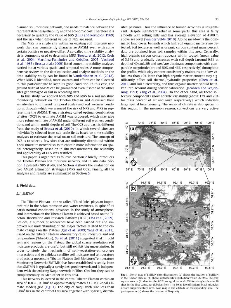
Fig. 1. Sketch map of SMTMN sites distribution: (a) shows the location of SMTMNin the Tibetan Plateau; (b) shows detailed site distribution within SMTMN. The graysquare area in (b) denotes the 0.25� sub-grid network. White triangles denote 30sites in the first campaign (labeled from 1 to 30 as identification), black trianglesdenote supplementary sites. Base map is the altitude of corresponding area. Thepentagram in (b) shows the location of Naqu city.

2. Field data

2.1. SMTMN

The Tibetan Plateau – the so called ‘‘Third Pole’’ plays an impor-tant role in the Asian monsoon and water resources. In spite of itsharsh natural conditions, advances in the study of atmosphere-land interaction on the Tibetan Plateau is achieved based on the Ti-betan Observation and Research Platform (TORP) (Ma et al., 2009).Besides, a number of researches have been carried out and im-proved our understanding of the major factors related to the cli-mate changes on the Plateau (Qin et al., 2009; Yang et al., 2011).Based on the Tibetan Plateau observatory of soil moisture and soiltemperature (Tibet-Obs), Su et al. (2011) suggested that in coldsemiarid regions on the Plateau the global coarse resolution soilmoisture products are useful but still exhibit big uncertainties. Inorder to study the mechanism of soil–vegetation–atmosphereinteractions and to validate satellite soil moisture and temperatureproducts, a mesoscale Tibetan Plateau Soil Moisture/TemperatureMonitoring Network (SMTMN) has been established recently. Notethat SMTMN is typically a newly designed network and is indepen-dent with the existing Naqu network in Tibet-Obs, but they can becomplementary to each other in this area.

This network is located in the central Tibetan Plateau within anarea of 100 � 100 km2 to approximately match a GCM (Global Cli-mate Model) grid (Fig. 1). The city of Naqu with size less than6 km2 lies in the center of this area, together with sparsely distrib-

uted pastures. Thus the influence of human activities is insignifi-cant. Despite significant relief in some parts, this area is fairlysmooth with rolling hills and has average elevation of 4500 mabove sea level (van der Velde, 2010). Alpine meadow is the dom-inated land cover, beneath which high soil organic matters are de-tected. Soil texture as well as organic carbon content mass percentdata are obtained from soil samples within this area. Generally,high organic carbon content appears within topsoil (mean valueof 3.6%) and gradually decreases with soil depth (around 0.6% atdepth of 40 cm). Silt and sand are dominant components with com-parable magnitude (around 50% and 46%, respectively) throughoutthe profile, while clay content consistently maintains at a low va-lue less than 10%. Note that high organic matter content may sig-nificantly affect soil thermal/hydraulic properties (Chen et al.,2012) and soil dielectricity, and thus organic matters should be ta-ken into account during sensor calibration (Jacobsen and Schjon-ning, 1993; Yang et al., 2004). On the other hand, all these soiltexture components show notable variability (about 13% and 20%for mass percent of silt and sand, respectively), which indicateslarge spatial heterogeneity. The seasonal climate is also special inthis region. In the monsoon season, convections are very active

94 L. Zhao et al. / Journal of Hydrology 482 (2013) 92–104

in this high altitude area and frequently appear in terms of showeror hailstorm. From May to October, this area receives its bulk pre-cipitation accumulated to around 400 mm (Su et al., 2011) whilevery little precipitation during winter. Besides, soil thawing andfreezing are typical phenomena, occurring around May andNovember, respectively.

The SMTMN network was accomplished through two installa-tion campaigns in 2010 and 2011, respectively. In the first cam-paign, 30 sites were deployed since July, 2010 (see whitetriangles in Fig. 1b). These sites are deployed along four branchesof the national/provincial roads. In the second campaign, another20 sites were added into SMTMN in July, 2011 (see black trianglesin Fig. 1b). The sensors are capacitance probes (EC-TM for the first30 sites and 5TM for the 20 new sites) provided by Decagon De-vices (http://www.decagon.com/), which can simultaneously mea-sure volumetric water content (VWC) and soil temperature with anaccuracy of ±3% VWC/±1 �C and resolution of 0.1% VWC/0.1 �C formineral soil. Note that only the liquid water content is measuredwithin frozen soils during winter. At each site, four sensors areused to monitor soil moisture/temperature at depths of 0–5 cm,10 cm, 20 cm, and 40 cm, respectively. Measuring time interval isset to 30 min, and each record reflects the average state of soil overthe past half-hour. The new sites installed during the second cam-paign help to form a denser observing network that contains 22sites within a 25 � 25 km2 area. This sub-grid network is expectedto be a reference site of the International Soil Moisture Network(Dorigo et al., 2011) and thus it was designed to match the pixelof currently ongoing or planned satellite microwave observingmissions. With this concept, the SMTMN can serve as a validationsite, e.g. for the Advanced Microwave Scanning Radiometer for theEarth Observing System (AMSR-E) (Kawanishi et al., 2003), the SoilMoisture and Ocean Salinity (SMOS) mission (Kerr et al., 2001), theMETOP-A Advanced Scatterometer (ASCAT) (Bartalis et al., 2007),and the upcoming Soil Moisture Active Passive (SMAP) Mission(Entekhabi et al., 2010). In addition, both soil ring samples and dis-turbed soil samples were collected at each site with an incrementof five centimeters from 0 to 45 cm for sensor calibration, whichwas accomplished with the gravimetric method in laboratory.

2.2. Temporal scales of soil moisture time series

According to the length of monitoring time window, data for thefirst 30 sites is available from August 1st, 2010 to September 20th,2011, while data for the newly added sites is only from July 10th,2011 to September 20th, 2011. The latter has relative short dura-tion and thus is not long enough for either spatiotemporal analysisor validation. Therefore, analyses on NRS, MRS, and OCS are onlyconducted based on the observations of the first 30 sites alongthe four branches of this area (hereafter referred to as ‘‘cross’’ area).

Different spatial/temporal studies require distinct temporalscales of soil moisture observations. Firstly, satellite passive micro-wave sensors have a revisit period of about several days and theobservation is taken at certain time point, thus its validation needsa higher temporal interval (e.g. half-hourly) for ground measure-ments (e.g., SMOS records at around 6:00 and 18:00 of local solartime in ascending and descending mode (Kerr et al., 2010)). Be-sides, for coarse scale long term study (e.g., drought monitoring),the soil moisture data is often averaged into daily or even largertemporal scales for evaluation. Therefore, it is valuable to conductthe spatiotemporal analyses of soil moisture data on various tem-poral scales, including half-hourly, daily, and monthly, etc. How-ever, considering the limited length of time series in the ‘‘cross’’area, this study presents analyses at a 10-days scale (10 d) insteadof the monthly scale. For each site, the half-hourly time series isthe original measurements, and the daily/10 d time series is di-rectly averaged from the half-hourly one. Note that within

SMTMN, some areas are rugged and have relatively higher eleva-tion (see Fig. 1b), which may cause problems in validations of landsurface models and remote sensing products. This makes theupscaling of point observations to a coarse scale be a crucial issue.Yet this is outside the scope of this study, and we simply take the30 sites-averaged soil moisture observations as areal mean soilmoisture (AMSM) of the ‘‘cross’’ area.

3. Spatiotemporal analyses and random sampling

3.1. Spatiotemporal characteristics

In the following analyses, the near-surface (0–5 cm) soil mois-ture observations were used. Fig. 2a–c shows the 30 sites-averagedsoil moisture time series (ave) for three temporal scales (half-hourly, daily, and 10 d) in the ‘‘cross’’ area. To demonstrate the spa-tial variability, the standard deviation (std) and coefficient of vari-ation (CV) among these 30 sites are also calculated and shown inFig. 2.

Some spatiotemporal features can be detected, as follows:

(a) For all three temporal scales, all variables (average soil mois-ture, std, and CV) show obvious seasonal variations. Thisphenomenon is strongly correlated with precipitation andsoil temperature (see Fig. 2d, where TRMM_daily is the quar-ter degree TRMM_3B42_daily rainfall data provided by theTropical Rainfall Measuring Mission (TRMM) (Kummerowet al., 1998), and ave_TM05 is the 30 sites-averaged dailymean in situ near-surface soil temperature observations).Besides, the within day variations are smoothed out whendaily and 10 d temporal scales are used.

(b) Both average soil moisture and CV show great temporal fluc-tuations. In contrast, std appears to be more stable(�0.1 m3 m�3) than the other two.

(c) Under wetter surface conditions corresponding to higheraverage soil moisture, CV shows a lower value, while stdshows a relative higher value, and vice versa. These charac-teristics are consistent with previous studies (Famigliettiet al., 2008; Owe et al., 1982; Vereecken et al., 2007), inwhich CV is empirically expressed as exponential functionof mean field soil moisture, and std is at a maximum valuein the mid-range of observed moisture.

According to soil wetness conditions, spatiotemporal variationcharacteristics, and topsoil frozen status, the whole monitoringtime window is artificially divided into three time periods(Fig. 2: T1 – August 2010–October 2010, T2 – November 2010–May 2011, and T3 – June 2011–September 2011). T1 and T3 haverelative higher near-surface soil water content in summer, with alot of precipitation events (see Fig. 2d); while T2 has lower liquidsoil water content in winter, with frozen soil in the surface layer.Note that around November and May in T2, there are some obviousdaily fluctuations caused by diurnal freezing–thawing process.

3.2. Random sampling – NRS analyses

3.2.1. MethodIn this study, the number of required sites (NRS) is obtained

through random sampling analysis. This method does not requireany assumption of sampling statistical distribution, and is highlyrecommended by Wang et al. (2008). Besides, RMSD (root meansquare difference) of time series between average of sampled sitesand AMSM can be simply used to assess the performance of sam-ples and then determine the value of NRS (Brocca et al., 2010).

Fig. 2. (a–c) Time series of 30 sites-averaged soil moisture (ave) in ‘‘cross’’ area with standard deviation (std) and coefficient of variation (CV) for half-hourly, daily, and 10 dscales, respectively, (d) the spatial averaged near-surface soil temperature (ave_TM05) and TRMM3B42 daily rainfall (TRMM_daily). T1, T2, and T3 denote periodscorresponding to different soil wetness conditions.

L. Zhao et al. / Journal of Hydrology 482 (2013) 92–104 95

RMSD can be considered as function of number of sampled sitesand is calculated after

RMSDn ¼

ffiffiffiffiffiffiffiffiffiffiffiffiffiffiffiffiffiffiffiffiffiffiffiffiffiffiffiffiffiffiffiffiffiffiffiffiffiffiffiffiffiffiffiffiPMj¼1

1n

Pni¼1hij � hj

� �2

M

sð1Þ

hj ¼1N

XN

i¼1

hij ð2Þ

where n is number of sampled sites in one subset; 1n

Pni¼1hij and hj

are average of soil moisture measurement of selected i sites (subsetmean) and average of all the site-observations (AMSM) at time j;respectively; N is the total number of sites; and M is the total num-ber of observations over a period.

Specially, for a certain temporal scale analysis during randomsampling, the population is observations of the 30 sites (N = 30).The maximum number of subsets in each sampling loop is set asmmax = 1000. Construction of the random sampling approach is asfollows:

Step 1: Prepare sampling population, set n = 1, m = 1. Here n isthe number of sampled sites within a subset and m denotesthe mth sampled subset.Step 2: Randomly select n sites from population into the mthsubset. Calculate correlation coefficient (Rn,m) and root meansquare difference (RMSDn,m) between time series of subset-mean and AMSM.Step 3: Set m = m + 1, repeat step 2 until m = mmax. Calculateboth the mean value and standard deviation

Rn stdðRÞnRMSDn stdðRMSDÞn

� �� �for correlation coefficient and root

mean square difference of all the mmax subsets.Step 4: Set n ¼ nþ 1, repeat step 2 to step 4 until n ¼ N toexplore all the possible number of sampled sites.

When the random sampling finished, R stdðRÞRMSD stdðRMSDÞ

� �can be

considered as a function of n. Then NRS can be identified by certaincriterion of mean and standard deviation of RMSD and R.

96 L. Zhao et al. / Journal of Hydrology 482 (2013) 92–104

3.2.2. ResultAnalyses on NRS of near-surface (0–5 cm) soil moisture were

conducted for half-hourly, daily, and 10 d temporal scales with re-spect to all time periods (T1, T2, and T3). Fig. 3a1–a3, b1–b3 showsthe general relationship between statistical performance indices(R, RMSD) and number of sampled sites (NSS) (the half-hourly scaleis excluded for conciseness). At the beginning, for all time periodsof both daily and 10 d temporal scales, large RMSD (or low R) is ob-tained with small NSS, while its value decreases (or increases) rap-idly with increasing NSS, as expected. Then both RMSD and Rchange very little and approach relative stable values with furtherincreased NSS until NSS = 30. Correspondingly, the standard devia-tion of both RMSD and R show a similar trend. This is reasonablebecause larger number of samples may yield more accurate esti-mate of AMSM.

Fig. 3a4 and b4 integrate statistical performance indices of alltime periods together. For both daily and 10 d temporal scales,the correlations between R (RMSD) and NSS in T1 are very similarwith the one in T3. Meanwhile, under the same NSS, wetter condi-tions (T1 and T3 in summer) have relative larger RMSD, lower R, aswell as larger standard deviation than dryer condition (T2 in win-

Fig. 3. Relationship of RMSD and R for the near-surface soil moisture with the number odeviation; (a4) and (b4) show the comparison of the relationship for different periods.

ter). This is perhaps because (1) all the sites maintain extremelylow level of liquid soil water content in the surface layer duringT2; and (2) less occurrence of precipitation events in winter, sincepattern of rainfall is the main impact that results in large soil mois-ture spatial variability.

A certain value of R and RMSD can be used as criterion to deter-mine NRS. As introduced before, the soil moisture sensor has anaccuracy of ±3%VWC. However, the measuring uncertainties canbe reduced to some extent by averaging measurements of severalsites. Therefore in this study a compromised criterion of R P 0.99and RMSD6 0.02 m3 m�3 is used. As shown in Table 1, all the threetemporal scales require nearly the same NRS for a certain time per-iod. This reveals that NRS is insensitive to temporal scales. T1 andT3 require relative consistent larger values of NRS while T2 needssmaller ones, indicating NRS is sensitive to soil wetness conditions.Generally, NRS = 13 is required throughout all the time periods,which can guarantee a robust and stable estimate of AMSM forthe ‘‘cross’’ area.

Subjected to spatial scales, accuracy levels, and the total de-ployed sites, the estimated NRS values can be various. By usingsimilar random sampling analysis, Wang et al. (2008) obtained

f sampled sites at daily (a1–a3) and 10 d (b1–b3) scales, with bars for ±1 standard

Table 1Number of required sites (NRS) for the ‘‘cross’’ area.

NRS T1 T2 T3

Half-hourly 12 9 13Daily 11 8 1310 d 10 7 12

L. Zhao et al. / Journal of Hydrology 482 (2013) 92–104 97

NRS = 38 under confidence level of 95% and relative error of 5% in a55 m-scale plot. Brocca et al. (2010) found NRS ranging between 4and 15 at the field scale and increasing to 40 at the catchment scalewithin an absolute error of 0.02 m3 m�3. Recently, in the study ofBrocca et al. (2012), the authors also suggested two sites per100 km2 are adequate to estimate the areal mean temporal patternwith RMSD less than 0.02 m3 m�3. In spite of these, the reliability ofNRS estimated in this study and its sensitivity to total number ofsites in the network is further discussed in the next sub-sections.

3.2.3. Discussion on reliability of NRSTo study the reliability of estimated NRS, a supplementary

experiment was conducted, i.e., the random sampling process inSection 3.2.1 was repeated by specifying number of sampled sitesas n = 13 in one subset with mmax = 10,000 to cover more sampledsubsets. Fig. 4a shows the frequency distribution of number of sub-sets with respect to different levels of RMSD value in the experi-ment. Statistically, 76.56% and 94.83% of subsets in total haveRMSD within 0.02 m3 m�3 and 0.03 m3 m�3, respectively. In fact,during the random sampling process there are always some sub-sets which contain sites very close to each other and locate withina small part of the ‘‘cross’’ area, and as a consequence yield largeRMSD. However, this influence can be eliminated by artificially uni-formly deploying the sites within the area in practical.

Strictly speaking, the determination of NRS is sort of subjectiveissue and the random sampling process may contain risk. A differ-ent criterion is expected to generate a distinct value of NRS. Basedon the random sampling in Section 3.2.1, we counted the numberof subsets that perform with statistical indices beyond criterionwith various levels (RMSD: 0.005 m3 m�3 ? 0.030 m3 m�3) toquantify the risk during random sampling. Fig. 4b shows the gen-eral result. For a specified NSS, the more rigorous of the criterion(lower RMSD), the larger percentage of unqualified subsets exists,and vice versa. On the other hand, for a specified percentage value

Fig. 4. Results of reliability and risk study on random sampling when applied to the nnumber of sampled subsets and the cumulative frequency for a specified 13 sampled spercentage) out of criterion with various levels of RMSD (units for RMSD: m3 m�3).

(e.g., 20%), smaller NSS is valid with a relaxed criterion (largerRMSD). With increasing NSS, the cost on field work will increaseas well, while more accurate estimate of AMSM can be achievedand thus reduce the risk in reliability. Nevertheless, one can setup an appropriate criterion to get NRS, based on practical require-ments and conditions of the target field.

3.2.4. Discussion on the population sizeIn this study, we used 30 sites within the ‘‘cross’’ area to conduct

the NRS analyses. However, different networks may have variousnumber of sites, i.e., denser or coarser than SMTMN. This makesit necessary to know how the results would behave if fewer siteswere installed in the same spatial scale. To elaborate on this issue,a sensitivity study on the number of sites in the population wasimplemented.

We repeated the random sampling process in Section 3.2.1 withsize of population varying from 15 to 29 that are chosen based onthe existing 30 sites. To eliminate the influence of randomness dur-ing the selection of population, a prior random sampling processwas used. Taking population size of 20 as an example, firstly, weobtained 10 groups of 20 sites randomly sampled from the original30 sites, and secondly, we carried out similar analyzing steps inSection 3.2.1 for each group. NRS value was obtained by usingthe same criterion as the 30 sites condition (R P 0.99 andRMSD 6 0.02 m3 m�3). Finally, the minimum, maximum, and meanNRS value of 10 groups for three time periods are calculated. Notethat only the daily temporal scale is analyzed.

Table 2 shows the overall results. Generally, the relationship be-tween soil wetness conditions and NRS values appears the same asthe case with the 30 sites condition. T2 requires relative lower NRSthan T1 and T2, indicating the soil wetness condition should be ta-ken into account when estimating NRS. Furthermore, with increas-ing size of population (15 ? 30), the NRS value increases slightly,especially for T1 and T3. This may be due to the representativenessof less sites within the network in capturing the areal mean soilmoisture. As shown in Fig. 3a1 and a3, the standard deviation ofRMSD for T1 and T3 still have remarkable values when number ofsampled sites is over 13. In contrast, the mean RMSD for T2 con-verges to a small value with low standard deviation, which meanstime series averaged over different number of sites (i.e. the size ofpopulation) is close to the average over 30 sites, thus the NRS valueobtained from a less population size is comparable to the one in the

ear-surface soil moisture measurements. (a) Frequency distribution histogram ofites; (b) relationship between number of sampled sites and number of subsets (in

Table 2Number of required sites (NRS) with respect to the size of population for the ‘‘cross’’ area. Analyzed is the daily mean near-surface soil moisture.

Population size NRS_T1 NRS_T2 NRS_T3

Min Max Mean Min Max Mean Min Max Mean

15 8 9 9 6 8 7 9 10 1016 8 9 9 6 7 7 8 11 1017 8 10 9 6 7 7 7 11 1018 8 10 9 6 8 7 9 11 1019 9 10 9 7 8 7 9 11 1020 9 10 9 7 8 7 8 11 1021 9 11 10 7 7 7 9 12 1122 9 11 10 7 7 7 10 12 1123 9 11 10 7 8 8 10 12 1224 10 11 11 7 8 7 11 12 1225 10 11 11 7 8 8 11 13 1226 9 11 10 7 8 7 11 13 1227 10 12 11 7 8 8 11 13 1228 10 11 11 7 8 8 12 13 1329 11 11 11 8 8 8 12 14 1330 11 11 11 8 8 8 13 13 13

98 L. Zhao et al. / Journal of Hydrology 482 (2013) 92–104

30 sites case. In spite of these, the estimated NRS values under dif-ferent population size conditions have the same magnitude, andthe representative issue is kind of problem with the criterion set-tings, as already discussed in Section 3.2.3.

The analyses on NRS will provide important guidance for theestablishment of future soil moisture networks. For a currentlyongoing network, another issue is to get reliable estimate of AMSMbased on existing sites. This is addressed in the following section.

4. AMSM estimate strategy

Two strategies are evaluated in estimating AMSM. One is basedon a single site, the so-called most representative site (MRS). Theother is a newly proposed approach called optimal combinationof sites (OCS).

4.1. Single site estimation

For an area with relative small spatial scale, soil moisture at dif-ferent locations is expected to be highly correlated with each other.It is likely to find a single site that can reflect the average near-sur-face wetness (Brocca et al., 2009). For larger spatial scales, inde-pendent studies found that one representative site is still able toestimate AMSM within an area of �200 km2 (Brocca et al., 2012)and �1000 km2 (Martínez-Fernández and Ceballos, 2005). Thismakes it interesting to investigate the feasibility of estimatingAMSM with a single site when spatial scale extending up to10,000 km2. In this study, the single site estimation is tested andevaluated based on the data collected from the Plateau SMTMN.

4.1.1. Time stability representationThe most representative site (MRS) is determined by time sta-

bility of each site through relative difference analyses. Vachaudet al. (1985) first introduced the time stability concept to identify‘‘representative’’ sites for AMSM estimation. In the analysis, time-invariant probability density functions are assigned to individuallocations using temporal analysis of the differences between ob-served time series of a single site and spatial average. Specifically,the relative difference (RD) is defined as

dij ¼hij � hj

hj; ð3Þ

where i = 1,2,3, . . . ,N (identification number of sites), j = 1,2,3, . . . ,M(number of observations over a period), and hj is spatial average attime j calculated after (2). The mean relative difference (MRD) and

standard deviation of relative difference (SDRD) for each site are cal-culated by

di ¼1M

XM

j¼1

dij ð4Þ

rðdiÞ ¼

ffiffiffiffiffiffiffiffiffiffiffiffiffiffiffiffiffiffiffiffiffiffiffiffiffiffiffiffiffiffiffiffiffiffiffiffiffiffiffiffiffi1

M � 1

XM

j¼1

ðdij � diÞ2vuut ð5Þ

MRD and the SDRD characterize closeness and precision of theestimation at a single site, respectively. Obviously, a ‘‘stable’’ and‘‘representative’’ site is identified by a low value of both rðdiÞand di. Particularly, the root mean square difference (RMSD) ofRD is computed (Jacobs et al., 2004) as

RMSDi ¼ffiffiffiffiffiffiffiffiffiffiffiffiffiffiffiffiffiffiffiffiffiffiffid2

i þ rðdiÞ2q

ð6Þ

RMSD provides a single metric to identify MRS. (6) and (1) can bemathematically proved equal to each other if the average time ser-ies of a subset in random sampling (Section 3.2.1) is treated as a sin-gle site observation.

4.1.2. Evaluation on MRS time stabilityThe relative difference approach is conducted independently for

all time periods and both the daily and 10 d temporal scales for thenear-surface soil moisture observations. Fig. 5 shows the rank ofsites that ordered by MRD with error bars of standard deviation.Generally, a relative dryer soil condition, i.e. sites that have nega-tive MRD, yields relative lower standard deviation. This is consis-tent with Jacobs et al. (2004). Meanwhile, the range of MRDvalues is quite large, especially for T2, as compared with previousstudies (Brocca et al., 2009, 2010; Cosh et al., 2004; Jacobs et al.,2004). According to Mittelbach and Seneviratne (2012), the spatialvariance of absolute soil moisture over time can be divided intotime-invariant (i.e. the temporal mean of a site) and time-varying(i.e. the temporal anomalies) components, and these two may haveseparate contributions. For T1 and T2, the large MRD range iscaused by both the time-invariant and time-varying components.The former is mainly due to high spatial heterogeneity within thisarea, and the latter is probably caused by inhomogenous precipita-tion. In contrast, the time-invariant contribution may be domi-nated during T2 since the soil moisture appears to have verylittle temporal variations in most times (see Fig. 2). Particularly,under very low liquid soil water content within frozen soil, theinfluence of spatial heterogeneity may be remarkably enlarged

Fig. 5. Rank ordered mean relative difference with its standard deviation (vertical bar) and RMSD for different temporal scales and periods. Analyzed are the near-surface soilmoisture measurements.

L. Zhao et al. / Journal of Hydrology 482 (2013) 92–104 99

through normalization of RD-calculation, and therefore significantlarger MRD and SDRD are obtained in T2.

For a specified period, both daily and 10 d temporal scale anal-yses obtained approximately the same rank of sites. Besides, thepotential MRSs suggested by the lowest RMSD are consistent forboth daily and 10 d temporal scales (Fig. 5), indicating that MRSidentified according to time stability is insensitive to temporalscales.

For a specified temporal scale, RMSD has the same magnitudeand trend with MRD. This is because MRD in (6) is the dominantvariable in calculating RMSD, while SDRD has approximately thesame value for different sites. Meanwhile, the differences betweenRMSD and MRD are even larger during T2 because of larger SDRDunder dryer soil conditions, especially for site-2 (Fig. 5a2 andb2). On the other hand, different time periods have different ranksof sites, and also suggest a distinct MRS. According to Fig. 5, theMRS identified by rank of RMSD is site-30 for T1 and T3, and site-16 for T2. This suggests that the time stability identified MRS issensitive to soil wetness conditions. This result is inconsistent with

Brocca et al. (2010), in which the time stability of sites seems to benot affected by extreme wet or dry conditions.

Based on relative difference analyses, Jacobs et al. (2004) usedfive locations having di values closest to zero to predict AMSM,whereas De Lannoy et al. (2007) used different relationships andmethods to render a single site (MRS) to be more representativefor AMSM. However, this kind of empirical approach may resultin over-fitting and sacrifice the internal physical mechanism aswell. In this study, we simply conducted cross-validation amongthe two potential MRSs to evaluate the reliability of a single sitein estimating AMSM. This is similar to the study of Grayson andWestern (1998) in which the AMSM was assumed equal to a singlesite measurement.

Fig. 6 shows comparison of daily mean soil moisture betweenMRSs estimates and 30 sites averaged AMSM. Obviously, neithersite-16 nor site-30 which was identified from a specified time per-iod can give reliable estimate for other time period(s). MRS ob-tained through relative difference analyses is limited to only ashort time period or some certain soil wetness conditions. For

Fig. 6. Cross-comparison between daily time series of areal mean near-surface soil moisture and MRSs estimates.

100 L. Zhao et al. / Journal of Hydrology 482 (2013) 92–104

the long run of SMTMN, due to variable soil wetness conditions, asingle site may not be able to give robust and reliable estimate ofAMSM.

4.2. A few sites combination estimate

Since it is risky to estimate AMSM from a single site, we pro-posed to estimate AMSM based on the combination of a few sites,which can be considered as a compromise between cost on fieldwork and risk in reliability.

4.2.1. MethodFor the newly proposed optimal combination of sites (OCS), we

chose a combination with five sites for evaluation and validation.The sensitivity to the number of selected sites is given in Sec-tion 4.2.3. Similar to the NRS analyses, RMSD is calculated betweenAMSM and averaged time series of selected five sites. The analysisexhausted all the possible combinations of five sites, i.e. a numberof C5

30 ¼ 142;506 combinations in total. All the combinations are

Table 3List of the top 10 combinations ranked by performance index of RMSD and their ranks inscale.

ID_com n1 n2 n3 n4 n5 T1 + T2 + T3 T1

RMSD Rank R2 MD R

(a) Daily52029 3 7 12 18 20 0.007 19 0.990 �0.002 0128986 11 14 22 24 29 0.007 475 0.980 �0.002 0106769 7 14 18 20 27 0.007 847 0.977 �0.003 080108 5 7 16 20 26 0.007 1691 0.970 0.001 0112145 8 11 20 22 27 0.007 1000 0.973 �0.002 0128999 11 14 22 27 30 0.007 3672 0.988 �0.006 0128957 11 14 21 24 28 0.007 32 0.989 0.000 080081 5 7 16 18 20 0.008 362 0.979 �0.001 0106226 7 13 18 22 27 0.008 1849 0.972 �0.003 0108003 7 17 20 24 26 0.008 372 0.979 0.001 0

(c) 10 d106769 7 14 18 20 27 0.005 51 0.997 �0.002 0105492 7 12 17 24 26 0.005 29 0.995 0.000 052029 3 7 12 18 20 0.006 71 0.997 �0.002 0105709 7 12 21 27 29 0.006 727 0.994 �0.002 013513 1 7 9 20 22 0.006 1081 0.983 0.000 0128986 11 14 22 24 29 0.006 2024 0.985 �0.002 0112181 8 11 21 22 27 0.006 895 0.991 �0.003 0102460 7 9 16 20 27 0.006 711 0.994 �0.001 036832 2 8 22 23 28 0.006 379 0.991 �0.002 0108003 7 17 20 24 26 0.006 121 0.993 0.002 0

ID_com: the original identification number of all combinations; n1–n5: sites identificatiospecified time periods and temporal scale, R2: determination coefficient, MD: mean diff

marked with an identification number (ID) and ranked by RMSDvalue from the smallest to the largest. Thus the combinations withhigher ranks perform relative better than others in estimatingAMSM. In fact, there are so many combinations in total that thetop hundreds of combinations perform very close to each otherand any of them may be the possible OCS. Besides, each potentialcombination is likely to have different ranks in three time periods.Therefore, a mean root mean square difference for the whole per-iod is simply calculated after

RMSD ¼ RMSDT1 þ RMSDT2 þ RMSDT3

3ð7Þ

where RMSDTi corresponds to time period Ti. And the newly calcu-lated RMSD is expected to be a more suitable index that can reflectthe performance of combinations throughout all the time periods.

4.2.2. Near-surface AMSM estimation based on five sites combinationTable 3 listed the top 10 combinations with the smallest value

of RMSD for both daily and 10 d temporal scales and the corre-

individual time periods (bold): (a) for daily temporal scale, and (b) for 10 d temporal

T2 T3

MSD Rank R2 MD RMSD Rank R2 MD RMSD

.006 838 0.986 0.006 0.008 395 0.983 �0.003 0.007

.008 84 0.983 0.000 0.007 1053 0.980 �0.004 0.008

.008 736 0.974 �0.001 0.008 284 0.982 �0.001 0.007

.009 2215 0.975 0.001 0.009 26 0.988 0.000 0.006

.008 2775 0.968 0.001 0.009 65 0.992 0.004 0.006

.010 1213 0.971 �0.001 0.008 16 0.990 0.001 0.006

.006 2481 0.974 0.003 0.009 1340 0.976 0.000 0.009

.007 5215 0.960 �0.002 0.010 121 0.983 0.001 0.007

.009 2072 0.976 �0.005 0.009 91 0.983 0.001 0.007

.007 2311 0.972 0.003 0.009 606 0.988 �0.002 0.008

.003 1302 0.988 0.002 0.006 1326 0.985 0.001 0.006

.003 13456 0.960 �0.005 0.010 45 0.994 �0.001 0.003

.004 1597 0.986 �0.001 0.006 1349 0.982 0.000 0.006

.005 9 0.996 0.000 0.003 2815 0.989 0.005 0.007

.006 525 0.989 �0.001 0.005 658 0.995 0.004 0.005

.006 72 0.995 0.002 0.004 1058 0.987 0.000 0.006

.005 2555 0.986 �0.004 0.007 210 0.993 0.002 0.004

.005 47 0.996 �0.001 0.003 2678 0.985 0.001 0.007

.005 6814 0.988 0.002 0.008 117 0.995 �0.002 0.004

.004 2751 0.991 0.001 0.007 1073 0.991 �0.001 0.006

n number in specified combination, Rank: rank of corresponding combination for aerence (m3 m�3), RMSD: root mean square difference (m3 m�3).

L. Zhao et al. / Journal of Hydrology 482 (2013) 92–104 101

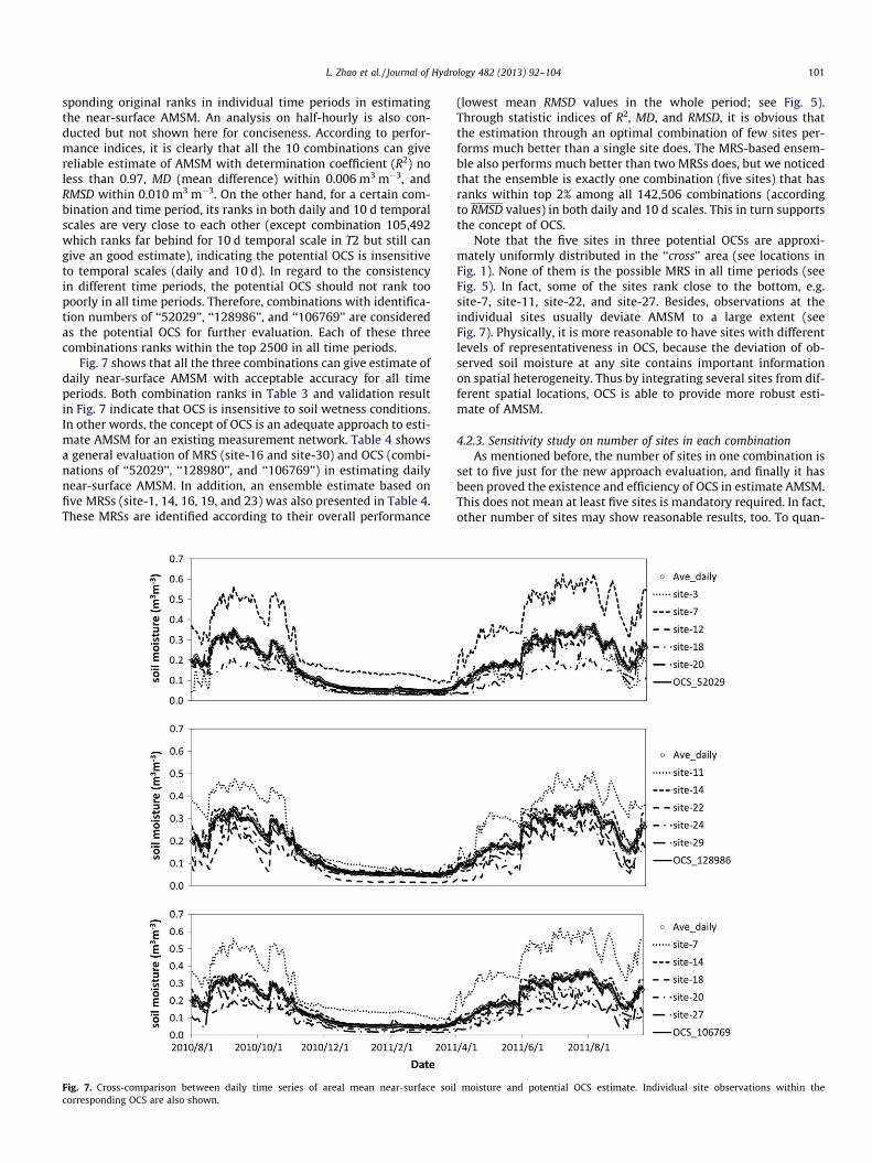
sponding original ranks in individual time periods in estimatingthe near-surface AMSM. An analysis on half-hourly is also con-ducted but not shown here for conciseness. According to perfor-mance indices, it is clearly that all the 10 combinations can givereliable estimate of AMSM with determination coefficient (R2) noless than 0.97, MD (mean difference) within 0.006 m3 m�3, andRMSD within 0.010 m3 m�3. On the other hand, for a certain com-bination and time period, its ranks in both daily and 10 d temporalscales are very close to each other (except combination 105,492which ranks far behind for 10 d temporal scale in T2 but still cangive an good estimate), indicating the potential OCS is insensitiveto temporal scales (daily and 10 d). In regard to the consistencyin different time periods, the potential OCS should not rank toopoorly in all time periods. Therefore, combinations with identifica-tion numbers of ‘‘52029’’, ‘‘128986’’, and ‘‘106769’’ are consideredas the potential OCS for further evaluation. Each of these threecombinations ranks within the top 2500 in all time periods.

Fig. 7 shows that all the three combinations can give estimate ofdaily near-surface AMSM with acceptable accuracy for all timeperiods. Both combination ranks in Table 3 and validation resultin Fig. 7 indicate that OCS is insensitive to soil wetness conditions.In other words, the concept of OCS is an adequate approach to esti-mate AMSM for an existing measurement network. Table 4 showsa general evaluation of MRS (site-16 and site-30) and OCS (combi-nations of ‘‘52029’’, ‘‘128980’’, and ‘‘106769’’) in estimating dailynear-surface AMSM. In addition, an ensemble estimate based onfive MRSs (site-1, 14, 16, 19, and 23) was also presented in Table 4.These MRSs are identified according to their overall performance

Fig. 7. Cross-comparison between daily time series of areal mean near-surface soicorresponding OCS are also shown.

(lowest mean RMSD values in the whole period; see Fig. 5).Through statistic indices of R2, MD, and RMSD, it is obvious thatthe estimation through an optimal combination of few sites per-forms much better than a single site does. The MRS-based ensem-ble also performs much better than two MRSs does, but we noticedthat the ensemble is exactly one combination (five sites) that hasranks within top 2% among all 142,506 combinations (accordingto RMSD values) in both daily and 10 d scales. This in turn supportsthe concept of OCS.

Note that the five sites in three potential OCSs are approxi-mately uniformly distributed in the ‘‘cross’’ area (see locations inFig. 1). None of them is the possible MRS in all time periods (seeFig. 5). In fact, some of the sites rank close to the bottom, e.g.site-7, site-11, site-22, and site-27. Besides, observations at theindividual sites usually deviate AMSM to a large extent (seeFig. 7). Physically, it is more reasonable to have sites with differentlevels of representativeness in OCS, because the deviation of ob-served soil moisture at any site contains important informationon spatial heterogeneity. Thus by integrating several sites from dif-ferent spatial locations, OCS is able to provide more robust esti-mate of AMSM.

4.2.3. Sensitivity study on number of sites in each combinationAs mentioned before, the number of sites in one combination is

set to five just for the new approach evaluation, and finally it hasbeen proved the existence and efficiency of OCS in estimate AMSM.This does not mean at least five sites is mandatory required. In fact,other number of sites may show reasonable results, too. To quan-

l moisture and potential OCS estimate. Individual site observations within the

Table 4Statistical performance indices of two MRSs (site-16, site-30), ensemble based on fiveMRSs, and three OCS selections (‘‘52029’’, ‘‘128986’’, and ‘‘106769’’) in estimatingdaily averaged areal mean soil moisture.

MRS MRS ensemble OCS

Site-16 Site-30 52029 128986 106769

R2 0.946 0.931 0.991 0.996 0.996 0.996MD 0.006 0.019 0.002 0.002 �0.001 0.000RMSD 0.029 0.034 0.010 0.007 0.007 0.007

R2: determination coefficient, MD: mean difference (m3 m�3), RMSD: root meansquare difference (m3 m�3).

102 L. Zhao et al. / Journal of Hydrology 482 (2013) 92–104

tify this issue, we implemented a sensitivity study on number ofcombined sites when varying from 1 to 8, and counted the numberof combinations that qualified under different levels of RMSD va-lue. Since previous part of this study has suggested the potentialOCS is insensitive to both soil wetness conditions and temporalscales, only daily soil moisture time series are used, and RMSD iscalculated throughout the whole time period for only once.

The sensitivity study results are shown in Table 5. Clearly, for aspecified number of sites in one combination, the total number ofcombinations increases with RMSD value. Meanwhile, for a speci-fied RMSD value, the number of qualified combinations (percent-age of all combinations in total) increases with number of siteswithin one combination, except the case for n = 1 that is similarto the study of MRS because no single site exists even withRMSD = 0.020 m3 m�3. Similar to the reliability study of NRS, thedetermination of number of sites in OCS is also subjective. In fact,when put looser requirement (e.g. larger RMSD) into practice, evenOCS with less than five sites may exist. Alternatively, when morethan five sites are selected, more potential OCS may appear. Inother words, researchers may have more choice in maintaining soilmoisture network in the wild.

4.2.4. Extended application of OCS to multi-depthPrevious studies clearly addressed the difficulty in finding a sin-

gle location with large time stability to characterize AMSM, andthis study further shows that MRS is sensitive to soil wetness con-ditions. In addition, since the time stability of locations is usuallyhighly variable within the soil profile (Hu et al., 2010), the effi-ciency of a single site in AMSM estimation is often questionedwhen applied to multi-depth of soil (Guber et al., 2008; Heathmanet al., 2009; Tallon and Si, 2004). However, the foregoing result onOCS has indicated the existence of large amount of potential com-binations in estimating near-surface AMSM with predeterminedaccuracy. This leads to an issue on how well the OCS can character-ize multi-depth AMSM. To evaluate this issue, the OCS estimationapproach is applied to multi-layer observations of the SMTMN.Number of sites in one combination is also set to five. Note thatsince site-1 and site-2 within SMTMN do not have sensor measure-

Table 5Number (percentage) of combinations within different criteria of RMSD valu

RMSD n = 1 (%) n = 2 (%) n = 3 (%) n = 4 (%

0.0040.0060.008 0.010.010 0.130.012 0.07 1.310.014 0.89 4.700.016 0.69 3.60 9.870.018 2.07 7.12 16.730.020 4.37 11.90 23.80

Units for RMSD: m3 m�3.

ments at depth of 20 cm and 40 cm, only observations of two lay-ers at depth 0–5 cm and 10 cm are used for validation.

Table 6 listed the top 10 combinations ranked by their overallperformance in estimating AMSM for both the first (0–5 cm) andthe second layer (10 cm). All these combinations can give robustAMSM estimate with determination coefficient no less than 0.990and RMSD within 0.009 m3 m�3 for 0–5 cm layer and0.007 m3 m�3 for 10 cm depth. Note that first, RMSD value for thesecond layer is in average less than the ones for the surface layer,which may be due to lower spatiotemporal variability within dee-per soils (Bogena et al., 2010; Rosenbaum et al., 2012); second,none of these top 10 combinations are included in the top 10 oneswhen only the surface layer soil moisture are considered(Table 3a), indicating there are many possible combinations ofOCS when five sites are specified. Anyway, this supplementaryanalysis has verified the feasibility of applying OCS for multi-depthAMSM estimation.

5. Summary and conclusions

Ground soil moisture monitoring network is necessary in vali-dating near-surface soil moisture products that estimated throughland surface model, satellite remote sensing, and land data assim-ilation at a grid scale. For decades, some pioneer researches havemade great progress in spatiotemporal analyses to get high accu-rate in situ measurement of areal mean soil moisture, and mostof them focused on the study of number of required sites (NRS)and the most representative sites (MRS). In this study, similaranalyses are conducted based on a newly established Tibetan-Plateau Soil Moisture/Temperature Monitoring Network (SMTMN).The large spatial scale, high elevation, typical land cover, and var-iable meteorological conditions as well as frozen-thawing pro-cesses make this area an ideal and valuable base for the relevantstudies.

The random sampling method is used to assess the number ofrequired sites (NRS). The relative difference analyses are intro-duced to study time stability of sites and then to identify the mostrepresentative site (MRS). Besides, a so-called optimal combinationof sites (OCS) approach is proposed to estimate AMSM throughseveral sites with a number far less than NRS. For the scientificrequirement, the original time series of 30 sites observations inthe ‘‘cross’’ area are artificially averaged into three temporal scales(half-hourly, daily, and 10-days) and divided into three time peri-ods that stands for different soil wetness conditions. Primary re-sults are as follows:

(a) NRS is insensitive to temporal scale but sensitive to soil wet-ness conditions. Larger NRS is obtained during summertimes when precipitation is dominant and higher soil watercontent maintains in topsoil. Generally NRS = 13 is obtainedunder criterion of R P 0.99 and RMSD 6 0.02 m3 m�3

es.

) n = 5 (%) n = 6 (%) n = 7 (%) n = 8 (%)

0.00 0.00 0.020.03 0.16 0.53 1.360.78 2.22 4.68 8.314.14 8.38 13.60 19.4910.47 17.20 24.00 30.5818.56 26.45 33.62 40.0426.69 34.78 41.85 48.0133.96 42.05 48.95 54.89

Table 6Statistical performance indices of top 10 OCS in estimating multi-depth daily averaged areal mean soil moisture.

ID_com n1 n2 n3 n4 n5 0–5 cm 10 cm

Rank R2 MD RMSD Rank R2 MD RMSD

57311 3 11 14 22 29 25 0.996 �0.0038 0.0078 121 0.995 0.0019 0.00599394 1 5 8 12 16 48 0.996 �0.0016 0.0080 115 0.995 0.0018 0.0059

128904 11 14 20 22 24 88 0.995 �0.0015 0.0083 35 0.995 0.0019 0.0055106227 7 13 18 22 28 64 0.995 �0.0006 0.0081 82 0.997 �0.0012 0.0058107220 7 15 18 20 23 205 0.994 �0.0003 0.0087 7 0.996 0.0001 0.0050106778 7 14 18 21 27 16 0.995 0.0000 0.0076 1161 0.992 �0.0007 0.0071128956 11 14 21 24 27 29 0.995 �0.0019 0.0078 733 0.993 �0.0009 0.0069112181 8 11 21 22 27 17 0.996 �0.0030 0.0076 1375 0.993 0.0011 0.0072

81053 5 8 11 21 27 89 0.994 �0.0017 0.0083 369 0.995 �0.0030 0.006552030 3 7 12 18 21 109 0.994 0.0013 0.0084 290 0.993 �0.0013 0.0063

ID_com: the original identification number of all combinations; n1–n5: sites identification number in specified combination, Rank: individual rank of correspondingcombination for near-surface (0–5 cm) and the second layer (10 cm) soil moisture estimate; R2: determination coefficient, MD: mean difference (m3 m�3), RMSD: root meansquare difference (m3 m�3).

L. Zhao et al. / Journal of Hydrology 482 (2013) 92–104 103

throughout the sampling time window, and is less influ-enced by the number of the total sites within the network.Note that the determination of NRS is subjective to compro-mise between cost on field work and risk in reliability.

(b) In time stability study, relative dryer conditions yields lowerstandard deviation of relative difference (RD); while signifi-cant larger mean RD and standard deviation of RD aredetected during winter times when very low liquid watercontent within the frozen soil. Similar to NRS, time-stabilitydetermined MRS is insensitive to temporal scale but sensi-tive to soil wetness conditions. Evaluating the result of MRSsindicates that no single site can give robust estimate ofAMSM for the whole time period.

(c) The proposed OCS approach is adequate in estimating near-surface AMSM. The determination of OCS is relative insensi-tive to both soil wetness conditions and temporal scales.Compared to a single site, a combination of a few sites cangive more robust and reliable estimate of AMSM. These sitesare approximately spatially uniformly distributed and con-tain more information on spatial heterogeneity. In addition,an extended study has shown the feasibility of OCS approachin multi-depth AMSM estimation.

The analyses of NRS in this study provide important guidancefor the establishment of future soil moisture network in similar re-gions. Meanwhile, the result of OCS study is encouraging forSMTMN maintenance as well as for AMSM estimation. Due to lim-itations in length of time series, the analyses are only conductedwithin a total time period of 14 months. However, a further valida-tion is encouraged when new data become available. Based onSMTMN in situ observations, the soil moisture upscaling and satel-lite product validation is in progress and will be addressed in thenear future.

Acknowledgements

The Tibetan Plateau Soil Moisture/Temperature MonitoringNetwork was financially supported by CMA Special Fund for Scien-tific Research in the Public Interest (Grant No. GYHY201206008),Global Change Program of Ministry of Science and Technology ofChina (Grant No. 2010CB951703), and National Natural ScienceFoundation of China (Grant No. 41190083). The authors thankDrs. Bob Su (University of Twente), Toshio Koike (University of To-kyo), and Ichiro Kaihotsu (Hiroshima University) who have pro-vided constructive advices on the network, and the drivers whohelped in the field work of Tibetan-Plateau. The analysis part ofthis study is supported by China Scholarship Council (CSC) scholar-ship. The TRMM daily rainfall data used in this effort were acquired

as part of the activities of NASA’s Science Mission Directorate, andare archived and distributed by the Goddard Earth Sciences (GES)Data and Information Services Center (DISC).

References

Bartalis, Z. et al., 2007. Initial soil moisture retrievals from the METOP-A AdvancedScatterometer (ASCAT). Geophys. Res. Lett. 34 (20), L20401.

Betts, A.K., Ball, J.H., Beljaars, A.C.M., Miller, M.J., Viterbo, P.A., 1996. The landsurface–atmosphere interaction: a review based on observational and globalmodeling perspectives. J. Geophys. Res. – Atmos. 101 (D3), 7209–7225.

Bogena, H.R. et al., 2010. Potential of wireless sensor networks for measuring soilwater content. Vadose Zone J. 9 (4), 1002–1013.

Brocca, L., Melone, F., Moramarco, T., Morbidelli, R., 2009. Soil moisture temporalstability over experimental areas in Central Italy. Geoderma 148 (3–4), 364–374.

Brocca, L., Melone, F., Moramarco, T., Morbidelli, R., 2010. Spatial-temporalvariability of soil moisture and its estimation across scales. Water Resour.Res. 46 (2), W02516.

Brocca, L., Tullo, T., Melone, F., Moramarco, T., Morbidelli, R., 2012. Catchment scalesoil moisture spatial–temporal variability. J. Hydrol. 422–423, 63–75.

Chen, Y., Yang, K., Tang, W., Qin, J., Zhao, L., 2012. Parameterizing soil organiccarbon’s impacts on soil porosity and thermal parameters for Eastern Tibetgrasslands. Sci. China Earth Sci. 55 (6), 1001–1011.

Cosh, M.H., Jackson, T.J., Bindlish, R., Prueger, J.H., 2004. Watershed scale temporaland spatial stability of soil moisture and its role in validating satellite estimates.Rem. Sens. Environ. 92 (4), 427–435.

Crow, W.T. et al., 2012. Upscaling sparse ground-based soil moisture observationsfor the validation of coarse-resolution satellite soil moisture products. Rev.Geophys. 50, RG2002.

De Lannoy, G.J.M., Houser, P.R., Verhoest, N.E.C., Pauwels, V.R.N., Gish, T.J., 2007.Upscaling of point soil moisture measurements to field averages at the OPE3test site. J. Hydrol. 343 (1–2), 1–11.

Dorigo, W.A. et al., 2011. The international soil moisture network: a data hostingfacility for global in situ soil moisture measurements. Hydrol. Earth Syst. Sci. 15(5), 1675–1698.

Entekhabi, D. et al., 2010. The soil moisture active passive (SMAP) mission. Proc.IEEE 98 (5), 704–716.

Entekhabi, D., Rodrigueziturbe, I., Bras, R.L., 1992. Variability in large-scale water-balance with land surface atmosphere interaction. J. Clim. 5 (8), 798–813.

Entin, J. et al., 1999. Evaluation of global soil wetness project soil moisturesimulations. J. Meteor. Soc. Jpn. 77, 183–198.

Famiglietti, J.S. et al., 1999. Ground-based investigation of soil moisture variabilitywithin remote sensing footprints during the Southern Great Plains 1997(SGP97) Hydrology Experiment. Water Resour. Res. 35 (6), 1839–1851.

Famiglietti, J.S., Ryu, D., Berg, A.A., Rodell, M., Jackson, T.J., 2008. Field observationsof soil moisture variability across scales. Water Resour. Res. 44 (1), W01423.

Grayson, R.B., Western, A.W., 1998. Towards areal estimation of soil water contentfrom point measurements: time and space stability of mean response. J. Hydrol.207 (1–2), 68–82.

Guber, A.K. et al., 2008. Temporal stability in soil water content patterns acrossagricultural fields. CATENA 73 (1), 125–133.

Heathman, G.C., Larose, M., Cosh, M.H., Bindlish, R., 2009. Surface and profile soilmoisture spatio-temporal analysis during an excessive rainfall period in theSouthern Great Plains, USA. CATENA 78 (2), 159–169.

Henderson-Sellers, A., 1996. Soil moisture simulation: achievements of the RICE andPILPS intercomparison workshop and future directions. Global Planet Change 13(1–4), 99–115.

Hills, R.C., Reynolds, S.G., 1969. Illustrations of soil moisture variability in selectedareas and plots of different sizes. J. Hydrol. 8 (1), 27–47.

104 L. Zhao et al. / Journal of Hydrology 482 (2013) 92–104

Hu, W., Shao, M., Han, F., Reichardt, K., Tan, J., 2010. Watershed scale temporalstability of soil water content. Geoderma 158 (3–4), 181–198.

Hupet, F., Vanclooster, M., 2002. Intraseasonal dynamics of soil moisturevariability within a small agricultural maize cropped field. J. Hydrol. 261 (1–4), 86–101.

Jacobs, J.M., Mohanty, B.P., Hsu, E.-C., Miller, D., 2004. SMEX02: field scalevariability, time stability and similarity of soil moisture. Rem. Sens. Environ.92 (4), 436–446.

Jacobsen, O.H., Schjonning, P., 1993. A laboratory calibration of time-domainreflectometry for soil–water measurement including effects of bulk-density andtexture. J. Hydrol. 151 (2–4), 147–157.

Kawanishi, T. et al., 2003. The advanced microwave scanning radiometer for theearth observing system (AMSR-E), NASDA’s contribution to the EOS forglobal energy and water cycle studies. IEEE Trans. Geosci. Rem. Sens. 41 (2),184–194.

Kerr, Y.H. et al., 2001. Soil moisture retrieval from space: the Soil Moisture andOcean Salinity (SMOS) mission. IEEE Trans. Geosci. Rem. Sens. 39 (8), 1729–1735.

Kerr, Y.H. et al., 2010. The SMOS mission: new tool for monitoring key elements ofthe global water cycle. Proc. IEEE 98 (5), 666–687.

Koster, R.D. et al., 2004. Regions of strong coupling between soil moisture andprecipitation. Science 305 (5687), 1138–1140.

Kummerow, C., Barnes, W., Kozu, T., Shiue, J., Simpson, J., 1998. The Tropical RainfallMeasuring Mission (TRMM) sensor package. J. Atmos. Ocean Technol. 15 (3),809–817.

Ma, Y. et al., 2009. Recent advances on the study of atmosphere-land interactionobservations on the Tibetan Plateau. Hydrol. Earth Syst. Sci. 13 (7), 1103–1111.

Martínez-Fernández, J., Ceballos, A., 2005. Mean soil moisture estimation usingtemporal stability analysis. J. Hydrol. 312 (1–4), 28–38.

Mittelbach, H., Seneviratne, S.I., 2012. A new perspective on the spatio-temporalvariability of soil moisture: temporal dynamics versus time-invariantcontributions. Hydrol. Earth Syst. Sci. 16 (7), 2169–2179.

Montzka, C. et al., 2011. Hydraulic parameter estimation by remotely-sensed topsoil moisture observations with the particle filter. J. Hydrol. 399 (2011), 410–421.

Njoku, E.G., Jackson, T.J., Lakshmi, V., Chan, T.K., Nghiem, S.V., 2003. Soil moistureretrieval from AMSR-E. IEEE Trans. Geosci. Rem. Sens. 41 (2), 215–229.

Owe, M., Jones, E.B., Schmugge, T.J., 1982. Soil moisture variation patterns observedin hand county, South Dakota. JAWRA J. Am. Water Resour. Assoc. 18 (6), 949–954.

Qin, J., Yang, K., Liang, S., Guo, X., 2009. The altitudinal dependence of recent rapidwarming over the Tibetan Plateau. Clim. Change 97 (1), 321–327.

Reichle, R.H., Koster, R.D., Dong, J.R., Berg, A.A., 2004. Global soil moisture fromsatellite observations, land surface models, and ground data: implications fordata assimilation. J. Hydrometeorol. 5 (3), 430–442.

Reynolds, S.G., 1974. A note on the relationship between size of area and soilmoisture variability. J. Hydrol. 22, 71–76.

Rodell, M. et al., 2004. The global land data assimilation system. Bull. Am. Meteorol.Soc. 85 (3), 381–394.

Rosenbaum, U. et al., 2012. Seasonal and event dynamics of spatial soil moisturepatterns at the small catchment scale. Water Resour. Res. 48, W10544.

Su, Z. et al., 2011. The Tibetan Plateau observatory of plateau scale soil moisture andsoil temperature (Tibet-Obs) for quantifying uncertainties in coarse resolutionsatellite and model products. Hydrol. Earth Syst. Sci. 15, 2303–2316.

Tallon, L., Si, B., 2004. Representative soil water benchmarking for environmentalmonitoring. J. Environ. Inform. 4 (1), 31–39.

Vachaud, G., Passerat De Silans, A., Balabanis, P., Vauclin, M., 1985. Temporalstability of spatially measured soil water probability density function. Soil Sci.Soc. Am. J. 49 (4), 822–828.

van der Velde, R., 2010. Soil Moisture Remote Sensing Using Active Microwaves andLand Surface Modelling. PhD Thesis, University of Twente, 193 pp.

Vanderlinden, K. et al., 2012. Temporal stability of soil water contents: a review ofdata and analyses. Vadose Zone J..

Vereecken, H. et al., 2007. Explaining soil moisture variability as a function of meansoil moisture: a stochastic unsaturated flow perspective. Geophys. Res. Lett. 34(22), L22402.

Wang, C.M., Zuo, Q., Zhang, R.D., 2008. Estimating the necessary sampling size ofsurface soil moisture at different scales using a random combination method. J.Hydrol. 352 (3–4), 309–321.

Yang, K., Koike, T., Ishikawa, H., Ma, Y., 2004. Analysis of the surface energy budgetat a site of GAME/Tibet using a single-source model. J. Meteorol. Soc. Jpn. Ser. II82 (1), 131–153.

Yang, K. et al., 2011. Response of hydrological cycle to recent climate changes in theTibetan Plateau. Clim. Change 109 (3), 517–534.