Expert Systems with Applications 39 (2012) 2059–2066

Contents lists available at SciVerse ScienceDirect

Expert Systems with Applications

journal homepage: www.elsevier .com/locate /eswa

Satellite-based and mesoscale regression modeling of monthly air and soiltemperatures over complex terrain in Turkey

Fatih Evrendilek ⇑, Nusret Karakaya, Kerem Gungor, Guler AslanAbant Izzet Baysal University, Department of Environmental Engineering, 14280 Bolu, Turkey

a r t i c l e i n f o a b s t r a c t

Keywords:Air and soil temperaturesAncillary dataComplex terrainMODISSpatio-temporal modeling

0957-4174/$ - see front matter � 2011 Elsevier Ltd. Adoi:10.1016/j.eswa.2011.08.023

⇑ Corresponding author. Tel.: +90 374 2541000.E-mail addresses: fevrendilek@yahoo.com, fevren

lek), karakaya_n@ibu.edu.tr (N. Karakaya), keremgungaslan_g@ibu.edu.tr (G. Aslan).

Simple regression algorithms were developed to quantify spatio-temporal dynamics of minimum andmaximum air temperatures (Tmin and Tmax, respectively) and soil temperature for a depth of 0–5 cm(Tsoil-5cm) across complex terrain in Turkey using Moderate Resolution Imaging Spectroradiometer(MODIS) data at a 500-m resolution. A total of 762 16-day MODIS composites (127 images � 6 bands)between 2000 and 2005 were averaged over a monthly basis to temporally match monthly Tmin, Tmax,and Tsoil-5cm from 83 meteorological stations. A total of 60 (28 temporally averaged plus 32 time ser-ies-based) linear regression models of Tmin, Tmax, and Tsoil-5cm were developed using best subsets proce-dure as a function of a combination of 12 explanatory variables: six MODIS bands of blue, red, nearinfrared (NIR), middle infrared (MIR), normalized difference vegetation index (NDVI), and enhanced veg-etation index (EVI); four geographical variables of latitude, longitude, altitude, and distance to sea (DtS);and two temporal variables of month, and year. The best multiple linear regression models elucidated65% (RMSE = 5.9 �C), 65% (RMSE = 5.1 �C), and 57% (RMSE = 6.9 �C) of variations in Tmin, Tmax, andTsoil-5cm, respectively, under a wide range of Tmin (�34 to 25 �C), Tmax (0.2–47 �C) and Tsoil-5cm (�9 to40 �C) observed at the 83 stations.

� 2011 Elsevier Ltd. All rights reserved.

1. Introduction

Readily available satellite data over a wide range of spatial andtemporal scales have enhanced the capacity of predicting andmonitoring dynamics of climate variables in the face of increasedrates of human-induced disturbances. Near-surface air and soiltemperatures are the two important driving variables that influ-ence biogeochemical cycles of atmosphere–water–vegetation–landcontinuum (Cristobal, Ninyerola, & Pons, 2008; Mostovoy, King,Reddy, Kakani, & Filippova, 2006; Nagler et al., 2005). Complex ter-rains, and impracticality of installing high density weather stationsare limiting an accurate estimation of air and soil temperatures aswell as capturing a representative description of their spatio-tem-poral variability. Therefore, modeling spatio-temporal heterogene-ity of air and soil temperatures plays a vital role in determining thepredictive capability of mesoscale ecosystem models (Park,Feddema, & Egbert, 2005; Yang et al., 2006). With the launch ofthe Advanced Very High Resolution Radiometer (AVHRR) andModerate Resolution Imaging Spectroradiometer (MODIS) satelliteimagers came the ability to quantify mesoscale spatio-temporalestimates of air and soil temperatures (Vancutsem, Ceccato, Dinku,

ll rights reserved.

dilek@ibu.edu.tr (F. Evrendi-or76@gmail.com (K. Gungor),

& Connor, 2010; Wan, 2008). Regression models have been used toderive the best estimates of biophysical and climatic variables suchas photosynthetically active radiation, surface emissivity, net pri-mary production, and Land Surface Temperature from a combina-tion of multiple spectral bands and satellite-based indices(Steinberg & Goetz, 2009; Zhao, Running, & Nemani, 2006).

Daily MODIS Land Surface Temperature (LST) products underclear sky conditions were validated against in situ measurementdata, with the resultant accuracy of better than 1 �C in the rangefrom �10 to 50 �C (Huang, Li, & Lu, 2008; Wan, Zhang, & Zhang,2004). The development and validation of regression models usingMODIS LST and Sea Surface Temperature (SST) data resulted in rea-sonable agreement with in situ data from different ecosystems(Chavula, Brezonik, Thenkabail, Johnson, & Bauer, 2009; Ellicott,Vermote, Petitcolin, & Hook, 2009; Wan, 2008). However, thesemodeling approaches have necessitated the use of MODIS LST orSST products at 1 to 10 km spatial resolutions and been restrictedto clear sky conditions, thus rendering them difficult to apply tocomplex terrain. Motivation for this work was to explore to whatextent devising a simple modeling framework with a few variablesreadily available from satellite images has a practical utility, espe-cially over rather complex and vast terrain having a limited num-ber of sites with conventional meteorological observations. Theobjective of this study was, therefore, to develop simple algorithmsto quantify monthly minimum and maximum air temperatures

2060 F. Evrendilek et al. / Expert Systems with Applications 39 (2012) 2059–2066

(Tmin and Tmax, respectively), and monthly mean soil temperaturesfor a 5-cm depth (Tsoil-5cm) over Turkey using meteorological andMODIS data between 2000 and 2005, along with ancillary informa-tion about altitude, latitude, longitude, and distance to sea (DtS) ata 500-m resolution.

2. Materials and methods

2.1. Study region

Turkey (36–42�N and 26–45�E) encompasses parts of Europe,Asia, Caucasia and the Middle East regions and is surrounded bythe Black Sea in north, the Aegean Sea in west, and the Mediterra-nean Sea in south, thus having diverse biogeoclimatic regimes andcomplex terrains. The complex terrain of Turkey has an elevationrange from sea level to about 5100 m, with a mean elevation of1000 m. The prevailing climate is characterized by cool and warmtemperate, Mediterranean, boreal and alpine conditions. Accordingto the long-term mean climate data between 1968 and 2004 forTurkey, mean annual maximum and minimum air temperaturesrange from 45 �C in July in the southeastern region to �30 �C inFebruary in the eastern regions, respectively (TSMS, 2005). Meanannual precipitation varies from 258 mm in the central and south-eastern regions to 2220 mm in the northeastern Black Sea coasts.

2.2. Compilation and processing of data

Monthly data for Tmin, Tmax, and Tsoil-5cm between January 2000and September 2005 were obtained for Turkey from 83 meteoro-logical stations (TSMS, 2005) (Fig. 1). The air temperature valuesrefer to an observation height approximately 1.5 m above ground,and the soil temperature values to the observation depth

Fig. 1. Geographical distribution of 83 meteorological stations

approximately 5 cm below ground. Sixteen-day composite MODISdata at 500-m resolution (MOD13A1 product, Collection 4) wereobtained for the six-year period of February 2000 to December2005 from the EOS Data Gateway (NASA EOS, 2007). Four MODIStiles (h20v04, h20v05, h21v04, and h21v05) cover Turkey (zone35N; WGS84 datum). The MODIS data acquired in HierarchicalData Format (HDF) were imported to GeoTIFF format and repro-jected from the original Sinusoidal projection to the decimal de-grees (DD) projection (WGS 84) using the MODIS ReprojectionTool (MRT) 3.0a (MRT, 2004) and ERDAS Imagine 8.7 (Leica Geosys-tems, Norcross, GA), based on the resampling method of nearestneighbor.

The time series of the MODIS data were matched with the read-ily available climate data of monthly Tmin, Tmax, and Tsoil-5cm for thesix-year period of 24 February 2000 to 29 September 2005. The en-tire time series of the MODIS data included a total of 762 16-daycomposite images (127 images � 6 bands), with the following in-ter-annual distribution of the images: 20 in 2000, 22 in 2001, 23in 2002, 22 in 2003, 23 in 2004, and 17 in 2005. The six bands ofthe MODIS composite images include the two vegetation indicesof normalized difference vegetation index (NDVI) and enhancedvegetation index (EVI), and the four bands of red (620–670 nm),blue (459–479 nm), near infrared (NIR, 841–876 nm), and middleinfrared (MIR, 2105–2155 nm). The calculations of NDVI and EVIare as follows:

NDVI ¼ ðqNIR � qREDÞ

ðqNIR þ qREDÞ ð1Þ

EVI ¼ 2:5� ðqNIR � qREDÞðqNIR þ 6� qRED þ 7:5� qBLUE þ 1:0Þ ð2Þ

where qNIR, qRED and qBLUE are the reflectances in the NIR band, redband and blue band, respectively. The blue and red band

used in this study along the altitudinal gradient of Turkey.

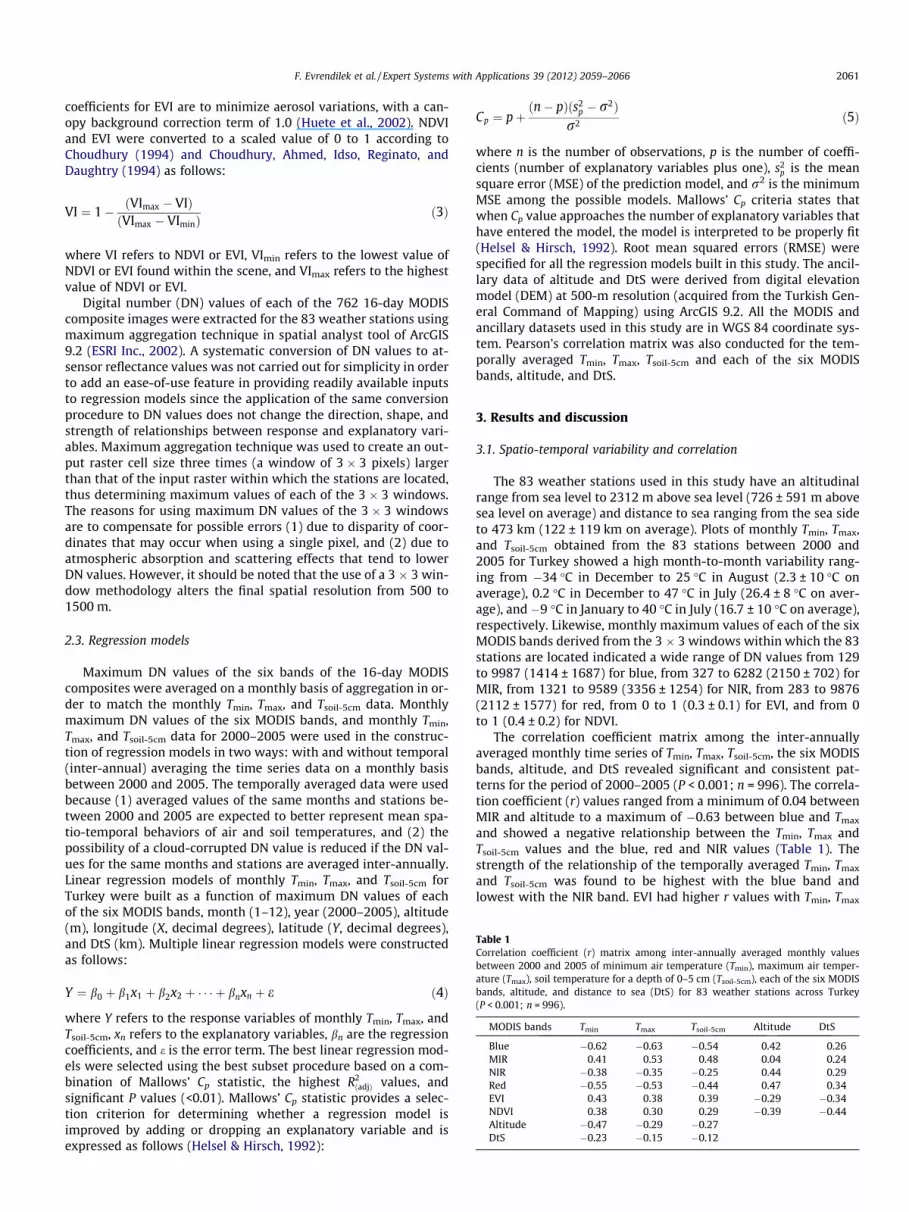
Table 1Correlation coefficient (r) matrix among inter-annually averaged monthly valuesbetween 2000 and 2005 of minimum air temperature (Tmin), maximum air temper-ature (Tmax), soil temperature for a depth of 0–5 cm (Tsoil-5cm), each of the six MODISbands, altitude, and distance to sea (DtS) for 83 weather stations across Turkey(P < 0.001; n = 996).

MODIS bands Tmin Tmax Tsoil-5cm Altitude DtS

Blue �0.62 �0.63 �0.54 0.42 0.26MIR 0.41 0.53 0.48 0.04 0.24NIR �0.38 �0.35 �0.25 0.44 0.29Red �0.55 �0.53 �0.44 0.47 0.34EVI 0.43 0.38 0.39 �0.29 �0.34NDVI 0.38 0.30 0.29 �0.39 �0.44Altitude �0.47 �0.29 �0.27DtS �0.23 �0.15 �0.12

F. Evrendilek et al. / Expert Systems with Applications 39 (2012) 2059–2066 2061

coefficients for EVI are to minimize aerosol variations, with a can-opy background correction term of 1.0 (Huete et al., 2002). NDVIand EVI were converted to a scaled value of 0 to 1 according toChoudhury (1994) and Choudhury, Ahmed, Idso, Reginato, andDaughtry (1994) as follows:

VI ¼ 1� ðVImax � VIÞðVImax � VIminÞ

ð3Þ

where VI refers to NDVI or EVI, VImin refers to the lowest value ofNDVI or EVI found within the scene, and VImax refers to the highestvalue of NDVI or EVI.

Digital number (DN) values of each of the 762 16-day MODIScomposite images were extracted for the 83 weather stations usingmaximum aggregation technique in spatial analyst tool of ArcGIS9.2 (ESRI Inc., 2002). A systematic conversion of DN values to at-sensor reflectance values was not carried out for simplicity in orderto add an ease-of-use feature in providing readily available inputsto regression models since the application of the same conversionprocedure to DN values does not change the direction, shape, andstrength of relationships between response and explanatory vari-ables. Maximum aggregation technique was used to create an out-put raster cell size three times (a window of 3 � 3 pixels) largerthan that of the input raster within which the stations are located,thus determining maximum values of each of the 3 � 3 windows.The reasons for using maximum DN values of the 3 � 3 windowsare to compensate for possible errors (1) due to disparity of coor-dinates that may occur when using a single pixel, and (2) due toatmospheric absorption and scattering effects that tend to lowerDN values. However, it should be noted that the use of a 3 � 3 win-dow methodology alters the final spatial resolution from 500 to1500 m.

2.3. Regression models

Maximum DN values of the six bands of the 16-day MODIScomposites were averaged on a monthly basis of aggregation in or-der to match the monthly Tmin, Tmax, and Tsoil-5cm data. Monthlymaximum DN values of the six MODIS bands, and monthly Tmin,Tmax, and Tsoil-5cm data for 2000–2005 were used in the construc-tion of regression models in two ways: with and without temporal(inter-annual) averaging the time series data on a monthly basisbetween 2000 and 2005. The temporally averaged data were usedbecause (1) averaged values of the same months and stations be-tween 2000 and 2005 are expected to better represent mean spa-tio-temporal behaviors of air and soil temperatures, and (2) thepossibility of a cloud-corrupted DN value is reduced if the DN val-ues for the same months and stations are averaged inter-annually.Linear regression models of monthly Tmin, Tmax, and Tsoil-5cm forTurkey were built as a function of maximum DN values of eachof the six MODIS bands, month (1–12), year (2000–2005), altitude(m), longitude (X, decimal degrees), latitude (Y, decimal degrees),and DtS (km). Multiple linear regression models were constructedas follows:

Y ¼ b0 þ b1x1 þ b2x2 þ � � � þ bnxn þ e ð4Þ

where Y refers to the response variables of monthly Tmin, Tmax, andTsoil-5cm, xn refers to the explanatory variables, bn are the regressioncoefficients, and e is the error term. The best linear regression mod-els were selected using the best subset procedure based on a com-bination of Mallows’ Cp statistic, the highest R2

ðadjÞ values, andsignificant P values (<0.01). Mallows’ Cp statistic provides a selec-tion criterion for determining whether a regression model isimproved by adding or dropping an explanatory variable and isexpressed as follows (Helsel & Hirsch, 1992):

Cp ¼ pþðn� pÞðs2

p � r2Þr2 ð5Þ

where n is the number of observations, p is the number of coeffi-cients (number of explanatory variables plus one), s2

p is the meansquare error (MSE) of the prediction model, and r2 is the minimumMSE among the possible models. Mallows’ Cp criteria states thatwhen Cp value approaches the number of explanatory variables thathave entered the model, the model is interpreted to be properly fit(Helsel & Hirsch, 1992). Root mean squared errors (RMSE) werespecified for all the regression models built in this study. The ancil-lary data of altitude and DtS were derived from digital elevationmodel (DEM) at 500-m resolution (acquired from the Turkish Gen-eral Command of Mapping) using ArcGIS 9.2. All the MODIS andancillary datasets used in this study are in WGS 84 coordinate sys-tem. Pearson’s correlation matrix was also conducted for the tem-porally averaged Tmin, Tmax, Tsoil-5cm and each of the six MODISbands, altitude, and DtS.

3. Results and discussion

3.1. Spatio-temporal variability and correlation

The 83 weather stations used in this study have an altitudinalrange from sea level to 2312 m above sea level (726 ± 591 m abovesea level on average) and distance to sea ranging from the sea sideto 473 km (122 ± 119 km on average). Plots of monthly Tmin, Tmax,and Tsoil-5cm obtained from the 83 stations between 2000 and2005 for Turkey showed a high month-to-month variability rang-ing from �34 �C in December to 25 �C in August (2.3 ± 10 �C onaverage), 0.2 �C in December to 47 �C in July (26.4 ± 8 �C on aver-age), and �9 �C in January to 40 �C in July (16.7 ± 10 �C on average),respectively. Likewise, monthly maximum values of each of the sixMODIS bands derived from the 3 � 3 windows within which the 83stations are located indicated a wide range of DN values from 129to 9987 (1414 ± 1687) for blue, from 327 to 6282 (2150 ± 702) forMIR, from 1321 to 9589 (3356 ± 1254) for NIR, from 283 to 9876(2112 ± 1577) for red, from 0 to 1 (0.3 ± 0.1) for EVI, and from 0to 1 (0.4 ± 0.2) for NDVI.

The correlation coefficient matrix among the inter-annuallyaveraged monthly time series of Tmin, Tmax, Tsoil-5cm, the six MODISbands, altitude, and DtS revealed significant and consistent pat-terns for the period of 2000–2005 (P < 0.001; n = 996). The correla-tion coefficient (r) values ranged from a minimum of 0.04 betweenMIR and altitude to a maximum of �0.63 between blue and Tmax

and showed a negative relationship between the Tmin, Tmax andTsoil-5cm values and the blue, red and NIR values (Table 1). Thestrength of the relationship of the temporally averaged Tmin, Tmax

and Tsoil-5cm was found to be highest with the blue band andlowest with the NIR band. EVI had higher r values with Tmin, Tmax

Table 2Best subsets regression models of inter-annually averaged monthly values (2000–2005) of minimum and maximum air temperatures (Tmin and Tmax), and soil temperature for adepth of 0–5 cm (Tsoil-5cm) as a function of location (X, Y), month, distance to sea (DtS), four spectral bands of monthly MODIS images (blue, red, NIR and MIR), and MODIS-derivedNDVI and EVI (n = 996; P < 0.001). Blue = 459–479 nm; red = 620–670 nm; NIR = near infrared (841–876 nm), MIR = middle infrared (2105–2155 nm), RMSE = root mean squareerror.

Responsevariable

Intercept X (longitude,decimaldegree)

Y (latitude,decimaldegree)

Month(1–12)

Altitude(m)

DtS(km)

Blue MIR NIR NDVI EVI R2

(%)R2

adj

(%)

Mallows’Cp

RMSE(�C)

Tmin (�C) 8.25 �0.004 38.1 765.1 7.8�5.29 �0.008 0.005 46.6 521.5 7.2�4.96 �0.005 �0.008 0.006 54.8 290.5 6.7�11.7 �0.006 �0.006 0.004 0.006 59.7 152.8 6.3�24.5 0.411 �0.008 �0.006 0.004 0.005 62.2 82.5 6.14.80 0.386 �0.698 �0.008 �0.006 0.003 0.005 63.3 53.6 6.01.96 0.534 �0.763 �0.007 �0.013 �0.006 0.004 0.005 64.1 30.1 5.92.39 0.517 �0.792 0.234 �0.007 �0.012 �0.006 0.004 0.005 64.7 14.9 5.94.99 0.514 �0.794 0.275 �0.007 �0.012 �0.006 0.004 0.004 �9.41 11.3 65.0 10.0 5.9

Tmax (�C) 31.7 �0.004 39.2 745.2 6.716.9 �0.008 0.006 52.7 358.7 5.99.69 �0.006 0.004 0.005 60.3 143.2 5.49.19 �0.002 �0.006 0.004 0.005 62.2 90.3 5.37.46 0.302 �0.002 �0.006 0.004 0.005 63.5 53.7 5.212.1 0.322 �0.002 �0.008 0.003 0.006 �7.56 64.2 34.2 5.112.5 0.318 �0.002 �0.008 �0.008 0.003 0.007 �9.04 64.7 19.8 5.17.76 0.148 0.308 �0.002 �0.011 �0.008 0.003 0.007 �9.15 65.0 12.8 5.110.1 0.145 �0.033 0.337 �0.002 �0.011 �0.007 0.003 0.006 �14.7 8.6 65.2 10.8 5.1

Tsoil-5cm

(�C)22.1 �0.004 28.9 712.6 8.91.67 �0.009 0.008 46.2 297.7 7.7�6.25 �0.008 0.004 0.007 52.2 153.2 7.3�6.99 �0.003 �0.008 0.005 0.008 55.0 87.4 7.1�8.75 0.306 �0.003 �0.008 0.005 0.008 55.9 67.2 7.0�15.6 0.223 0.296 �0.005 �0.007 0.005 0.007 56.5 53.4 7.05.55 0.204 �0.506 0.310 �0.004 �0.008 0.004 0.008 57.0 43.4 6.92.76 0.349 �0.567 0.291 �0.003 �0.012 �0.007 0.005 0.007 57.7 27.4 6.93.42 0.355 �0.478 0.308 �0.004 �0.014 �0.009 0.004 0.009 58.2 17.8 6.86.64 0.350 �0.511 0.356 �0.004 �0.013 �0.008 0.004 0.007 �17.

214.6 58.5 10.2 6.8

Frequencyof use(%)

43 32 46 71 32 100 75 89 21 11

2062 F. Evrendilek et al. / Expert Systems with Applications 39 (2012) 2059–2066

and Tsoil-5cm than did NDVI. Tmin, Tmax, and Tsoil-5cm had a negativecorrelation with both altitude and DtS in decreasing order of rvalues, respectively (Table 1). The increasing gradients along alti-tude and DtS can be considered to reflect an increase in the degreeof continentality as the interior and/or higher regions of Turkey aremore likely to have lower air and soil temperatures, wider air andsoil temperature ranges and drier conditions than the low andcoastal lands. Pape, Wundram, and Löffler (2009) found the samedirection of correlations in a high mountain environment as withthis study. Altitude and DtS were positively correlated with red,NIR, blue, and MIR and negatively correlated with NDVI, and EVIin decreasing order of r values.

3.2. Spatio-temporal analyses of Tmin, Tmax, and Tsoil-5cm with/withouttemporal averaging

The temporally averaged Tmin, Tmax and Tsoil-5cm for the 83 sta-tions were modeled as a function of each of the six temporallyaveraged MODIS bands, latitude, longitude, altitude, DtS, andmonth using best subsets regression that identifies the best-fittingmodels with as few explanatory variables as possible (Table 2). Inmodeling Tmin, Tmax and Tsoil-5cm time series without temporal aver-aging, the term ‘‘year’’ was included in addition to the above 11explanatory variables (Table 3). The 28 and 32 best subsets of lin-ear regression models with/without temporal averaging wererespectively selected in a way that the explanatory variables in-cluded in the models were additive in estimating the rate of changein the response variables. The rate and direction of change in the

response variables as expressed by the signs and coefficients ofthe explanatory variables showed a consistent pattern in termsof directions and magnitudes across the linear regression models,respectively (Tables 2 and 3). As can be seen in Tables 2 and 3,the standardized beta weights, and frequency of use of explanatoryvariables in the models assist in better understanding and compar-ing the importance of the predictors. The red band did not appearto be significant enough to be used in the 28 temporally averagedlinear regression models of the temporally averaged Tmin, Tmax andTsoil-5cm but was significant enough to be used in only one of the 32time series-based linear regression models. The two most fre-quently used explanatory variables were the blue and NIR bandsregardless of the building of the models with/without temporalaveraging. The two least frequently used explanatory variableswere EVI and NDVI in the temporally averaged regression modelsand the red band, and year in the time series-based regressionmodels (Tables 2 and 3). The temporally averaged regression mod-els had R2

ðadjÞ values ranging from 28.9% for Tsoil-5cm (RMSE = 8.9 �C)to 65.2% for Tmax (RMSE = 5.1 �C) (P < 0.001) (Table 2). R2

ðadjÞ valuesof the time series-based regression models ranged from 22.6% forTsoil-5cm (RMSE = 9.4 �C) to 61% for Tmin (RMSE = 6.3 �C) (P < 0.001)(Table 3).

The rate and direction of spatial changes in the temporally aver-aged Tmin, Tmax and Tsoil-5cm were quantified as, on average, 0.47 �C,0.15 �C, and 0.30 �C with every one unit increase in longitude;�0.76 �C, �0.03 �C, and �0.52 �C with every one unit increase inlatitude; �7 �C, �2 �C, and �4 �C with every 1 km increase in alti-tude; and �1.2 �C, �1.0 �C, and �1.3 �C with every 100 km increase

Table 3Best subsets regression models of monthly minimum and maximum air temperatures (Tmin and Tmax), and monthly soil temperature for a depth of 0–5 cm (Tsoil-5cm) as a functionof year, month, location (X, Y), distance to sea (DtS), four spectral bands of monthly MODIS images (blue, red, NIR and MIR), and MODIS-derived NDVI and EVI (n = 5607 for Tmin

and Tmax; n = 5589 for Tsoil-5cm; P < 0.001). Blue = 459–479 nm; red = 620–670 nm; NIR = near infrared (841–876 nm), MIR = middle infrared (2105–2155 nm), RMSE = root meansquare error.

Responsevariable

Intercept X (longitude,decimaldegree)

Y (latitude,decimaldegree)

Year(2000–2005)

Month(1–12)

Altitude(m)

DtS(km)

Blue MIR NIR Red NDVI EVI R2

(%)R2

adj

(%)

Mallows’Cp

RMSE(�C)

Tmin ( �C) 7.15 �0.003 31.3 4281.4 8.4�6.86 �0.007 0.006 41.5 2808.9 7.8�4.69 �0.005 �0.007 0.006 49.9 1601.3 7.2�10.0 �0.006 �0.005 0.004 0.005 55.0 868.2 6.8�22.5 0.403 �0.008 �0.005 0.004 0.005 57.4 530.3 6.6�24.6 0.398 0.389 �0.008 �0.005 0.004 0.004 58.9 305.6 6.57.84 0.374 �0.788 0.396 �0.008 �0.005 0.003 0.005 60.3 115.7 6.46.08 0.497 �0.851 0.390 �0.007 �0.011 �0.005 0.004 0.005 60.9 26.9 6.36.64 0.494 �0.890 0.400 �0.007 �0.010 �0.004 0.004 0.004 6.05 61.0 10.7 6.36.95 0.495 �0.883 0.405 �0.007 �0.010 �0.004 0.004 0.004 �2.37 8.93 61.0 9.6 6.3�0.4 0.495 �0.883 0.004 0.405 �0.007 �0.010 �0.004 0.004 0.004 �2.37 8.93 61.0 11.6 6.3

Tmax ( �C) 30.6 �0.003 29.7 3869.7 7.416.1 �0.007 0.006 44.1 1927.6 6.610.1 �0.005 0.004 0.005 51.7 904.4 6.17.53 0.454 �0.005 0.004 0.005 54.6 524.3 6.07.84 0.478 �0.003 �0.005 0.004 0.005 57.6 113.2 5.77.64 0.476 �0.002 �0.005 �0.005 0.004 0.005 57.8 87.9 5.79.92 0.476 �0.002 �0.006 �0.006 0.004 0.005 �4.62 58.1 55.0 5.76.33 0.114 0.473 �0.003 �0.008 �0.006 0.004 0.005 �4.75 58.2 32.1 5.76.63 0.114 0.483 �0.003 �0.008 �0.005 0.004 0.005 �7.75 6.33 58.3 23.6 5.7�87.8 0.114 �0.103 0.049 0.480 �0.002 �0.008 �0.006 0.004 0.004 0.002 �7.28 9.68 58.4 13.0 5.7

Tsoil-5cm

( �C)1.21 0.007 22.6 3870.7 9.41.41 �0.008 0.008 40.1 1734.1 8.2�5.0 �0.007 0.004 0.007 46.2 983.6 7.8�4.44 �0.004 �0.006 0.005 0.007 49.6 569.6 7.5�7.31 0.506 �0.004 �0.006 0.004 0.007 52.1 272.9 7.318.0 �0.628 0.512 �0.004 �0.006 0.004 0.007 52.9 179.5 7.310.4 0.195 �0.589 0.509 �0.005 �0.006 0.004 0.007 53.3 121.0 7.38.59 0.318 �0.652 0.503 �0.004 �0.011 �0.006 0.005 0.006 53.9 50.0 7.2�335 0.318 �0.651 0.171 0.514 �0.004 �0.011 �0.006 0.005 0.006 54.0 43.6 7.2�320 0.321 �0.616 0.164 0.513 �0.004 �0.012 �0.007 0.004 0.007 �3.13 54.1 35.9 7.2�324 0.321 �0.634 0.167 0.534 �0.004 �0.012 �0.006 0.004 0.006 �9.12 12.7 54.3 11.0 7.2

Frequencyof use(%)

47 38 16 63 72 41 97 81 91 3 25 19

Fig. 2. Spatially and temporally averaged values of minimum and maximum air temperatures (�C) (Tmin and Tmax, respectively), soil temperature (�C) for a depth of 0–5 cm(Tsoil-5cm), and six bands of MODIS data (NDVI, EVI, red, blue, NIR, and MIR) over Turkey for the period of 2000–2005. NDVI = normalized difference vegetation index;EVI = enhanced vegetation index; NIR = near infrared; MIR = middle infrared. Months 1–12 refer to January to December, respectively.

F. Evrendilek et al. / Expert Systems with Applications 39 (2012) 2059–2066 2063

2064 F. Evrendilek et al. / Expert Systems with Applications 39 (2012) 2059–2066

in DtS (km), respectively (the minus sign used indicates a negativerelationship). The monthly rate of changes in Tmin, Tmax and Tsoil-5cm

were, on average, 0.25 �C, 0.32 �C, and 0.31 �C, respectively. Themagnitude of spatio-temporal changes in Tmin, Tmax and Tsoil-5cm

did not appear to significantly differ between the temporally aver-aged and time series-based regression models. The annual rate ofchanges in the Tmin, Tmax and Tsoil-5cm time series were, on average,0.004 �C, 0.05 �C, and 0.17 �C, respectively.

In all the 60 linear regression models, the response variableshad consistently a negative relationship with blue, and NDVI anda positive relationship with MIR, NIR, and EVI. The rate and direc-tion of changes in Tmin, Tmax and Tsoil-5cm that are associated withthe four MODIS spectral bands were, on average, estimated at�0.006 �C, �0.007 �C, and �0.008 �C with every one unit increasein DN value of the blue band; 0.004 �C, 0.003 �C, and 0.005 �C withevery one unit increase in DN value of the MIR band; and 0.005 �C,0.006 �C, and 0.008 �C with every one unit increase in DN value ofthe NIR band, respectively. The rate of changes were determined tobe 11.3 �C, 8.6 �C, and 14.6 �C with every one unit increase in EVIand �9.4 �C, �10.1 �C, and �17.2 �C with every one unit increasein NDVI, based on the best MLR models of the temporally averagedTmin, Tmax and Tsoil-5cm, respectively. The temporally averaged andtime series-based regression models were close to one another interms of magnitudes of their NDVI and EVI coefficients (Tables 2and 3).

The regression coefficients for NDVI were negative in all themodels constructed in this study, a pattern consistent with resultsin the related literature (Goetz, 1997; Kawashima, Ishida,Minomura, & Miwa, 2000; Mallick et al., 2007; Prince, Goetz,Czajkowski, Dubayah, & Goward, 1998). This case shows a system-atic inverse relationship between Tmin, Tmax, and Tsoil-5cm andvegetation density, one of the most important factors that affectthe thermal environment near the ground, which may be explainedby variation in evapotranspiration associated with the availability ofwater when the vegetation density increases according toChoudhury (1994), Moran, Clarke, Inoue, and Vidal (1994), and Filloland Royer (2003). As quantified by the models, the monthly rate ofincreases/decreases in Tmin, Tmax, and Tsoil-5cm at a 500-m resolution

10

0

-10

0.60.550.500.450.40

30

20

10

NDVI

Tso

il-5c

mT

max

Tm

in

Fig. 3. Relationships between spatially and temporally averaged values of MODIS vevegetation index) and those of minimum and maximum air temperatures (�C) (Tmin andTurkey on a monthly basis for the period of 2000–2005.

as the vegetation density decreases/increases, respectively, repre-sents the trajectory and magnitude of impacts of green canopydensity on Tmin, Tmax, and Tsoil-5cm across Turkey. Unlike NDVI, EVIis highly sensitive to land cover/use types with high vegetationdensity and reduces the atmospheric noise of soil background andaerosols and was positive in all the regression models as reportedby the related literature (Hu, Jia, & Guo, 2009).

On average, R2ðadjÞ values for the monthly estimation of Tmin, Tmax,

and Tsoil-5cm across Turkey were higher by 3.4%, 6.8%, and 4.2% inthe temporally averaged models than the time series-based ones,respectively. The RMSE values in the monthly estimation of Tmin,Tmax, and Tsoil-5cm across Turkey were reduced through temporalaveraging by 0.4 �C, 0.6 �C, and 0.4 �C compared to the time ser-ies-based ones, respectively. Accuracy of both temporally averagedand time series-based linear regression models were significantlyimproved by the stepwise addition to the models of blue, NIRand MIR bands, respectively. The predictive power of the linearregression models also increased by introducing the ancillaryspace, time and VI data in the following general order of stepwiseaddition as explanatory variables: altitude, month, longitude,latitude, DtS, NDVI, EVI, and year. The variation of Tmin, Tmax, andTsoil-5cm with altitude quantified in all the models shows a patternsimilar to the standard temperature lapse rate of 4.5–6.5 �C km�1

(Jain, Goswami, & Saraf, 2008). It should be noted that accuracyof the 12 regression models (out of 60) that can be used for map-ping spatio-temporal distribution as can be seen in Tables 2 and3 can be also evaluated using cross-validation results from 360maps (5 models � 12 months � 6 years) and 84 maps (7 mod-els � 12 months), a question beyond the focus of this study.

3.3. Temporally and spatially averaged Tmin, Tmax and Tsoil-5cm timeseries

The temporally and spatially averaged Tmin, Tmax, Tsoil-5cm, NDVI,EVI and MIR displayed a similar unimodal response whereby thesevariables increase during spring, level off during summer, and de-crease during autumn (Fig. 2). The temporally and spatially aver-aged red and blue DN values showed a monthly opposite

0.500.450.400.350.30

40

30

20

0

EVI

getation indices (NDVI = normalized difference vegetation index; EVI = enhancedTmax, respectively), and soil temperature (�C) for a depth of 0–5 cm (Tsoil-5cm) over

F. Evrendilek et al. / Expert Systems with Applications 39 (2012) 2059–2066 2065

behavior of Tmin, Tmax, Tsoil-5cm, NDVI, EVI and MIR, while the DNvalues of the NIR band exhibited a bimodal behavior with two min-ima in April and October (Fig. 2). The best multiple non-linearregression models of the temporally and spatially averaged Tmin,Tmax, Tsoil-5cm and each of the MODIS bands were determined asfollows:

Tsoil-5cm ¼ �2:60þ 3:04 monthþ 0:7438 month2

� 0:0812 month3 R2adj ¼ 90:7%; RMSE ¼ 3:14; P < 0:001

� �

ð6Þ

Tmax ¼ 10:31þ 2:45 monthþ 0:621 month2

� 0:066 month3 R2adj ¼ 97:5%; RMSE ¼ 1:29; P < 0:001

� �

ð7Þ

Tmin ¼ �12:02þ 1:34 monthþ 0:814 month2

� 0:076 month3 R2adj ¼ 90:9%; RMSE ¼ 2:54; P < 0:001

� �

ð8Þ

NDVI ¼ 0:283þ 0:07 month

� 0:005 month2 R2adj ¼ 73:1%; RMSE ¼ 0:03; P ¼ 0:001

� �

ð9Þ

EVI ¼ 0:148þ 0:12 month� 0:012 month2

þ 0:0003 month3 R2adj ¼ 79:7%; RMSE ¼ 0:03; P ¼ 0:001

� �

ð10Þ

Red ¼ 3953� 680:9 monthþ 47:95 month2ðRadj

¼ 75:9%; RMSE ¼ 311:1; P 6 0:001Þ ð11Þ

Blue ¼ 3741� 851:1 month

þ 59:26 month2 R2adj ¼ 83:5%; RMSE ¼ 312:4; P < 0:001

� �

ð12Þ

NIR ¼ 2244þ 3462 month� 2341 month2 þ 644 month3

� 84:3 month4 þ 5:2 month5

� 0:122 month6 R2adj ¼ 86:5%; RMSE ¼ 128:2; P ¼ 0:007

� �

ð13Þ

MIR ¼ 1193þ 357:0 month

� 24:89 month2 R2adj ¼ 93:8%; RMSE ¼ 76:5; P ¼ 0:001

� �

ð14Þ

Eqs. (6)–(14) indicate that it is possible to, on average, pinpointnational-scale monthly behaviors of Tmin, Tmax, Tsoil-5cm, and MODISbands of NDVI, EVI, red, blue, NIR and MIR for Turkey. Relationshipsbetween the MODIS vegetation indices (NDVI and EVI) and monthlyTmin, Tmax and Tsoil-5cm were illustrated in Fig. 3. Cubic modelsdescribing a ‘‘peak and valley’’ pattern appeared to provide a goodfit to all the spatially and temporally averaged data, with R2

adj valuesof 64.2% and 73.9% for Tmin, 66.4% and 76.8% for Tsoil-5cm, and 75.1%and 82.4% for Tmax as a function of NDVI and EVI, respectively.

4. Conclusions

Under the wide Tmin, Tmax and Tsoil-5cm range from �34 to 25 �C,from 0.2 to 47 �C, and from �9 to 40 �C observed in the 83 stations,respectively, results of the simple regression algorithms derivedfrom the use of a combination of the six MODIS bands (blue, NIR,MIR, NDVI, EVI, and red), geographical variables (altitude, latitude,longitude, and DtS), and temporal variables (month, and year) ap-pear to be promising in the estimation of monthly Tmin, Tmax, andTsoil-5cm across the entire nation with complex terrain at a 1500-m resolution, especially given the fact that minimum and maxi-mum temperatures are often more difficult to model than meantemperatures. Out of the 60 linear regression models, the best onesaccounted for 65% (RMSE = 5.9 �C), 65% (RMSE = 5.1 �C), and 57%(RMSE = 6.9 �C) of variations in Tmin, Tmax, and Tsoil-5cm, respec-tively. Potential error sources in the models are most likely to stemfrom the lack of discrimination of clear-sky pixels from cloud pix-els, the time difference between the satellite overpass and themonthly Tmin, Tmax, Tsoil-5cm data, the spatial scale mismatch be-tween the MODIS data (500 m) and the point ground measure-ments, the radiometric and geometric precision of the MODISinstrument, atmospheric interferences, and reprojecting from sinu-soidal projection. However, potential errors were minimized usingnearest-neighbor resampling during reprojecting, and maximumaggregation technique (extraction of maximum values from a win-dow of 3 � 3 pixels) as well as temporally averaged values to re-duce the issues of cloud contamination, and atmosphericinferences. In addition, the exploration of interactive effects(non-linear relationships) among the 12 explanatory variables,and the addition to the regression algorithms of important bio-physical variables such as land use and cover dynamics, solar radi-ation, albedo, and evapotranspiration are most likely to improvethe performance of the regression models though the trade-off be-tween simplicity and predictive capability of the models is dis-torted against the model simplicity.

Acknowledgments

This research was financially supported by the Scientific andTechnological Research Council of Turkey (TUBITAK-TOVAG-104O550), and Abant Izzet Baysal University.

References

Chavula, G., Brezonik, P., Thenkabail, P., Johnson, T., & Bauer, M. (2009). Estimatingthe surface temperature of Lake Malawi using AVHRR and MODIS satelliteimagery. Physics and Chemistry of the Earth, 34, 749–754.

Choudhury, B. J. (1994). Synergism of multispectral satellite observations forestimating regional land surface evaporation. Remote Sensing of Environment, 49,264–274.

Choudhury, B., Ahmed, N., Idso, S., Reginato, R., & Daughtry, C. (1994). Relationsbetween evaporation coefficients and vegetation indices studied by modelsimulations. Remote Sensing of Environment, 50, 1–17.

Cristobal, J., Ninyerola, M., & Pons, X. (2008). Modeling air temperature through acombination of remote sensing and GIS data. Journal of Geophysical Research-Atmospheres, 113, D13106.

Ellicott, E., Vermote, E., Petitcolin, F., & Hook, S. J. (2009). Validation of a newparametric model for atmospheric correction of thermal infrared data. IEEETransactions on Geoscience and Remote Sensing, 47, 295–311.

ESRI Inc. (2002). ArcGIS 8.2. Redlands: ESRI Inc.Fillol, E. J., & Royer, A. (2003). Variability analysis of the transitory climate regime as

defined by the NDVI/Ts relationship derived from NOAA-AVHRR over Canada. InProceedings of IEEE international geoscience and remote sensing symposium,IGARSS (pp. 2863–2865).

Goetz, S. J. (1997). Multi-sensor analysis of NDVI, surface temperature andbiophysical variables at a mixed grassland site. International Journal of RemoteSensing, 18, 71–94.

Helsel, D. R., & Hirsch, R. M. (1992). Statistical methods in water resources.Amsterdam: Elsevier Science Publishers.

Hu, Y., Jia, G., & Guo, H. (2009). Linking primary production, climate and land usealong an urban–wildland transect: A satellite view. Environmental ResearchLetters, 4, 044009.

2066 F. Evrendilek et al. / Expert Systems with Applications 39 (2012) 2059–2066

Huang, C., Li, X., & Lu, L. (2008). Retrieving soil temperature profile by assimilatingMODIS LST products with ensemble Kalman filter. Remote Sensing ofEnvironment, 112, 1320–1336.

Huete, A., Didan, K., Miura, T., Rodreguez, E., Gao, X., & Ferreira, L. (2002). Overviewof the radiometric and biophysical performance of the MODIS vegetationindices. Remote Sensing of Environment, 83, 195–213.

Jain, S. K., Goswami, A., & Saraf, A. K. (2008). Determination of land surfacetemperature and its lapse rate in Satluj basin using NOAA data. InternationalJournal of Remote Sensing, 29, 3091–3103.

Kawashima, S., Ishida, T., Minomura, M., & Miwa, T. (2000). Relations betweensurface temperature and air temperature on a local scale during winter nights.Journal of Applied Meteorology, 39, 1570–1579.

Mallick, K., Bhattacharya, B. K., Chaurasia, S., Dutta, S., Nigam, R., Mukherjee, J., et al.(2007). Evapotranspiration using MODIS data and limited ground observationover selected agroecosystems in India. International Journal of Remote Sensing,28, 2091–2110.

Moran, M. S., Clarke, T. R., Inoue, V., & Vidal, A. (1994). Estimating crop water deficitusing the relation between surface-air temperature and spectral vegetationindex. Remote Sensing of Environment, 49, 246–263.

Mostovoy, G. V., King, R. L., Reddy, K. R., Kakani, V. G., & Filippova, M. G. (2006).Statistical estimation of daily maximum and minimum air temperatures fromMODIS LST data over the State of Mississippi. GIScience and Remote Sensing, 43,78–110.

MRT (2004). MODIS reprojection tool users guide. Release 3.2a, Department ofMathematics and Computer Science, South Dakota School of Mines andTechnology. South Dakota: USGS EROS Data Center.

Nagler, P. L., Scott, R. L., Westenburg, C., Cleverly, J. R., Glenn, E. P., &Huete, A. R. (2005). Evapotranspiration on western US rivers estimatedusing the enhanced vegetation index from MODIS and data from eddycovariance and Bowen ratio flux towers. Remote Sensing of Environment,97, 337–351.

NASA EOS (2007). Earth observing system data gateway. Available from: https://wist.echo.nasa.gov/api/.

Pape, R., Wundram, D., & Löffler, J. (2009). Modelling near-surface temperatureconditions in high mountain environments: An appraisal. Climate Research, 39,99–109.

Park, S., Feddema, J. J., & Egbert, S. L. (2005). MODIS land surface temperaturecomposite data and their relationships with climatic water budget factors in theCentral Great Plains. International Journal of Remote Sensing, 26, 1127–1144.

Prince, S. D., Goetz, S. J., Czajkowski, K., Dubayah, R., & Goward, S. N. (1998).Inference of surface and air temperature, atmospheric precipitable water andvapor pressure deficit using AVHRR satellite observations: Validation ofalgorithms. Journal of Hydrology (212/213), 231–250.

Steinberg, D. C., & Goetz, S. (2009). Assessment and extension of the MODIS FPARproducts in temperate forests of the eastern United States. International Journalof Applied Earth Observation and Geoinformation, 30, 169–187.

TSMS (2005). Monthly climate data. Ankara: Turkish State Meteorological Service.Vancutsem, C., Ceccato, P., Dinku, T., & Connor, S. J. (2010). Evaluation of MODIS

land surface temperature data to estimate air temperature in differentecosystems over Africa. Remote Sensing of Environment, 114, 449–465.

Wan, Z., Zhang, Y., & Zhang, Q. (2004). Quality assessment and validation of theMODIS global land surface temperature. International Journal of Remote Sensing,25, 261–274.

Wan, Z. (2008). New refinements and validation of the MODIS land-surfacetemperature/emissivity products. Remote Sensing of Environment, 112, 59–74.

Yang, F. H., White, M. A., Michaelis, A. R., Ichii, K., Hashimoto, H., Votava, P., et al.(2006). Prediction of continental-scale evapotranspiration by combining MODISand AmeriFlux data through support vector machine. IEEE Transactions onGeoscience and Remote Sensing, 44, 3452–3461.

Zhao, M., Running, S. W., & Nemani, R. R. (2006). Sensitivity of Moderate ResolutionImaging Spectroradiometer (MODIS) terrestrial primary production to theaccuracy of meteorological reanalyses. Journal of Geophysical Research, 111. G1.