Wind resource modelling in complex terrain using different mesoscale–

microscale coupling techniques

D. Carvalho, A. Rocha, C. Silva Santos, R. Pereira

ABSTRACT

Wind resource evaluation in two sites located in Portugal was performed using the mesoscale modelling system Weather Research and Forecasting (WRF)

and the wind resource analysis tool commonly used within the wind power industry, the Wind Atlas Analysis and Application Program (WAsP) microscale

model. Wind measurement campaigns were conducted in the selected sites, allowing for a comparison between in situ measurements and simulated wind,

in terms of flow characteristics and energy yields estimates.

Three different methodologies were tested, aiming to provide an overview of the benefits and limita - tions of these methodologies for wind resource

estimation. In the first methodology the mesoscale model acts like ‘‘virtual’’ wind measuring stations, where wind data was computed by WRF for both

sites and inserted directly as input in WAsP. In the second approach, the same procedure was followed but here the terrain influences induced by the

mesoscale model low resolution terrain data were removed from the simulated wind data. In the third methodology, the simulated wind data is extracted

at the top of the planetary boundary layer height for both sites, aiming to assess if the use of geostrophic winds (which, by definition, are not influenced by

the local terrain) can bring any improvement in the models performance.

The obtained results for the abovementioned methodologies were compared with those resulting from in situ measurements, in terms of mean wind

speed, Weibull probability density function parameters and production estimates, considering the installation of one wind turbine in each site. Results

showed that the second tested approach is the one that produces values closest to the measured ones, and fairly acceptable deviations were found using

this coupling technique in terms of estimated annual production. However, mesoscale output should not be used directly in wind farm sitting projects,

mainly due to the mesoscale model terrain data poor resolution. Instead, the use of mesoscale output in microscale models should be seen as a valid

alternative to in situ data mainly for preliminary wind resource assessments, although the application of mesoscale and microscale coupling in areas with

complex topography should be done with extreme caution.

Keywords:

Wind energy, Wind simulation, Mesoscale models, Microscale models, WRF, WAsP

1. Introduction

Energy is presently considered one of the most valuable com-

modities in the economical progress and wealth generation of a

country, being one of the main driving forces of industrial

-

development. Considering the escalating costs of the traditional

fossil energy sources, supported by the growing global demand

for energy production, an intensive search for alternative sources

of energy (preferably renewable ones) has been pursued in the re-

cent past. Among the several available renewable energy sources,

wind-derived energy is the one that has witnessed greatest growth

in the recent years. Presently, Portugal is one of the world leading

countries in terms of installed wind power and this growth is still

in progress. In 2011, Portugal was ranked in 10th place worldwide

and 5th place among European countries in terms of total wind en-

ergy installed capacity [1]. In 2010, Portugal was able to achieve an

18% quota of wind-derived energy in the total annual energy con-

sumption, outranked worldwide only by Denmark [2]. The current

and future expansion of the wind energy markets, combined with

the explosive growth of worldwide installed wind power over the

last decade and the progressive liberalization of electricity mar-

kets, poses several and new challenges to the wind power industry,

namely in determining the most appropriate sites for wind energy

exploration [3].

Although the use of this renewable energy source has been rap-

idly increasing worldwide, the lack of reliable and accurate wind

measured data in several areas of the globe is still hampering the

development of new wind energy projects, and this fact is particu-

larly serious in developing countries [4,5]. Currently, the state of

the art in wind resource assessment is based on classical methods

that use measured data recorded locally [6], and subsequently in-

serted as input in microscale models to assess the local wind re-

source. These methods are still the most reliable for an efficient

and realistic planning of potential wind farm sites, meaning higher

certainty in the expected available wind resource and lower asso-

ciated investment risks, which are key prerequisites for the suc-

cessful development of wind energy projects [7]. However,

measurement campaigns have some constraints, namely their high

costs, data quality/availability and the need to perform measure-

ments for a representative period, typically with a minimum dura-

tion of 1 year. Also, measurement campaigns may reveal that the

site has little wind energy potential, which will lead to the irrevers-

ible loss of a considerable amount of investment. Moreover, the

increasing evolution of the wind energy industry is bringing the

need to obtain a preliminary knowledge of the available wind re-

source at sites with few (or not at all) of local measurements. In

these sites, this preliminary knowledge of the local wind regimes

is of the utmost importance, at least in a preliminary stage in order

to help in the wind resource assessment process.

Considering these disadvantages of the wind measurement

campaigns together with the abovementioned growing needs of

the wind power industry, the potential benefits of an alternative

way to obtain reliable wind data for a spatial mapping and tempo-

ral distribution of the wind resource are obvious [8]. Numerical

weather prediction (NWP) mesoscale models, which consist of

atmospheric models that consider physical phenomena such as

frictional, thermal and convective effects, are a very powerful

and useful tool to simulate meteorological variables [9]. These

mesoscale models can provide ‘‘virtual’’ wind data sets that can

be used as input in microscale models, instead of using measured

wind data. In the recent past, mesoscale simulations have been

used in a considerable number of applications within the wind

power area: building wind resource maps in spatially large areas

(useful in large scale electrical grid planning and preliminary

assessment of potential wind energy exploration sites); computing

local long term climatologies to allow the assessment of the wind

variability and the representativeness of measurement campaigns

(typical for the majority of wind farm projects, in order to estimate

the expected annual energy production); and in the growing field

of wind power production short term forecasting (due to the need

to plan electrical grid balance). However, as with any numerical

simulation, the limitations of this approach should be carefully

considered on a case-by-case analysis. The use of mesoscale mod-

els as source of wind data offers, on one hand, advantages like: low

operational costs (most of the mesoscale models are freely avail-

able for download and the costs involved in their use are residual);

higher sampling resolution (both horizontal and vertical, allowing

the computation of virtual wind data sets for several sites at differ-

ent heights) when compared to wind measuring stations; and they

offer data sets with 100% of availability. On the other hand, there

are disadvantages due to the uncertainty associated to wind data

derived from these types of models: mesoscale models do not rep-

resent the real state of the atmosphere (like real observed mea-

surements do) because atmospheric simulation models are, by

definition, an approximation of the real atmosphere; the represen-

tation in mesoscale models of the terrain characteristics and phys-

ical processes that occur in the atmosphere are simplified.

Nevertheless, the use of mesoscale models as source of wind

data for wind resource mapping and/or assessment, either for di-

rect use in microscale models or for studies that do not require a

microscale level of detail (wind resource mapping for large areas,

for example), has been performed in the recent past with interest-

ing and promising results: [10] performed a wind resource map-

ping for Norway using the WRF and WAsP models, with results

that showed deviations in wind speed between 3% and 25%

(depending on the local terrain complexity); [11] built a wind atlas

for Egypt using the Karlsruhe Atmospheric Mesoscale Model

(KAMM) mesoscale model, with deviations in the simulated wind

speed between 5% and 10%, the latter for areas with high local ter-

rain complexity; [12] computed a wind atlas for Spain with the

Skiron mesoscale model, and the results showed a wind speed an-

nual bias of 1.87 m s-1 over simple terrain and annual bias of

2.5 m s-1 over complex terrain; for the Portuguese territory, [13]

assessed the wind resource with the WRF model for two distinct

sites (one located in a coastal area with low terrain complexity

and the other one situated in a mountainous area with high terrain

complexity), showing that the WRF model can reproduce the aver-

age wind speed with deviations below 5%; also, [14] conducted a

wind energy potential study for the Madeira island with two meso-

scale models (MM5 and NH3D), showing that mesoscale models

can successfully be applied to the wind resource mapping and

enhancing the contribution that these models can offer in the wind

resource prediction. Other interesting applications of mesoscale

models were found, such as to correct measurements by means

of long-term climatology [15] and for short-term wind power fore-

cast [16].

To determine if accurate mesoscale model-based wind power

resource assessments can be accomplished, three different meth-

ods to couple the mesoscale modelling system WRF with the

microscale model WAsP were compared. These methods were

tested for an area with high terrain complexity located in Portugal,

well known for its wind energy resource where several wind farms

are currently in operation and being one of the most important

Portuguese areas in terms of installed wind generating power.

The use of these methods in wind resource and production esti-

mates will be compared to the traditional methods that rely on

measured wind data.

2. Methodology

2.1. Wind measurement data sets

Data from two wind measuring stations was used in this work.

These wind measuring stations collected wind speed and direction

measurements at 60 m above ground level (a.g.l.), with a sampling

time resolution of 10 min. The measurements collected at these

stations during the year of 2008 were selected. This period was

considered due to its data availability and quality. The stations

are designated as stations A and B, and are located within the area

of the WRF simulation domain, in a central area of the Portuguese

mainland. However, the stations and the respective data belong to

private companies and their exact locations cannot be disclosed

due to data usage restrictions. Nevertheless, it is possible to show

in Fig. 1a their relative positions together with the local

topography.

The complexity of the terrain around a site can be objectively

measured through the ruggedness index or RIX, defined as the per-

centage fraction of the terrain within a certain distance from a spe-

cific site which is steeper than some critical slope, typically

considered around 0.3. A detailed description of the RIX index

can be found on [17], where basically the RIX is calculated for each

of a number of radii originating at the site (wind measuring station

or wind turbine). A flat site will then have a RIX of 0% and an ex-

treme complex (steep) site a RIX index of about 30%, meaning that

about one third of the terrain is steeper than the considered critical

slope of 0.3. This index can, therefore, be used as a site-specific

measure of the terrain complexity, and can describe with a high

degree of confidence the effects of local topography and rugged-

ness on the accuracy of WAsP predictions [17].

The two sites under scope in this work are characterized by dif-

ferent RIX values, meaning that they are located in areas with dif-

ferent terrain complexity. Fig. 1b shows the RIX spatial

distribution in the area surrounding stations A and B, being that

the site where is located station A has a RIX of 5.9% and station B site

RIX is 8.2%, showing that station A is located in a less complex site

than station B.

2.2. WRF mesoscale model

The mesoscale model selected to conduct the simulations is the

WRF (Advanced Research-ARW) version 3.0.1, a widely used meso-

scale model developed by the National Centre for Atmospheric Re-

search (NCAR). It currently represents the state of the art in

mesoscale modelling, and was originally released as a successor

to the long standing and well known Penn State/NCAR Fifth-Gener-

ation Mesoscale Model (MM5), sharing much of the same dynam-

ics and model physics. A detailed description of this model can be

found on [18].

The simulation domains are depicted in Fig. 2. The parent domain

(D1) has 90 km of spatial resolution, covering all of Iberian Penin-

sula. The first nested domain (D2), with a spatial resolution of

18 km, is centred in the Northern and Central Portugal. The second

nested domain (D3), with a spatial resolution of 3.6 km, includes

the location of the two sites here considered. The National Centres

for Environmental Prediction (NCEP) Final Operational Global Anal-

ysis, with 1° of spatial resolution (both in latitude and longitude) and

6 h of temporal sampling were used as initial and boundary data.

The complete year of 2008 was simulated with the WRF model,

and time series were extracted for the two sites where wind

Fig. 1. Wind measuring stations together with the altitude (a) and RIX (b) spatial

distributions. Fig. 2. WRF simulation domains.

measurement campaigns were conducted. The site that coincides

in location with the wind measuring station A is designated as site

1 and the site that coincides with the location of the wind measur-

ing station B is called site 2. For each site, two wind speed and

direction time series were computed: one at 60 m above ground le-

vel (a.g.l.), to match the height where the wind measurements took

place, and another one taken above the annual average height of

the PBL simulated by WRF for the year of 2008. All the virtual data

sets have a sampling rate of 10 min, to coincide also with the sam-

pling rate of the measurements.

2.3. WAsP microscale model

The microscale wind flow modelling was performed with the

WAsP code, version 9.1. WAsP is still the state of the art software

code for microscale modelling of wind resources and overall wind

assessment, with a 20 year track record of use by industry [6].

WAsP is especially designed for wind resource mapping, wind farm

micro-sitting and energy estimate purposes. WAsP requires, like

any atmospheric simulation model, initial conditions that are sup-

plied by observations or mesoscale simulations performed at one

or more sites. An important feature of the WAsP model is the abil-

ity of generalizing the measured observation at a local site into a

regional wind climate – the wind atlas. This model ingests the sup-

plied input data and builds a wind atlas, which consists in a

regional wind regime without the effects of the local terrain. For

that, the model first removes the topography and ruggedness ef-

fects of the supplied data and considers this ‘‘free wind’’ as repre-

sentative of the entire WAsP simulation domain. This concept of

wind atlas arises from the need to build a bridge between mea-

sured data in one site and the expected wind regime in a different,

but nearby, site. Once a wind atlas is established, the local wind

conditions at any site where the wind atlas is valid can be calcu-

lated. After the wind atlas computation, the wind regime for any

site inside its simulation domain will be computed doing the ex-

actly opposite process. In other words, WAsP takes the wind atlas

and re-inserts the terrain characteristics of the selected site to

compute its wind characteristics, assuming that the wind climate

at any specific site inside the domain may be calculated using

the regional climatology described by the wind atlas [19]. More de-

tail of this software can be found on [20].

2.4. Evaluation of the simulations accuracy

The comparison between the simulated and measured time ser-

ies is presented in terms of Weibull probability density function

(P.D.F.) parameters A (scale parameter), k (shape parameter), Um

(mean speed) and Umax (most probable wind speed), together with

the Weibull P.D.F. curves, annual wind roses of occurrence and of

available annual energy production (AEP).

The knowledge of the wind speed frequency distribution is a

key factor in the wind energy assessment. If this distribution is

known at a given site, then it can be described in terms of a Wei-

bull P.D.F., from which the energetic potential and economic feasi-

bility of this site can easily be obtained [4,5]. This distribution is

often used in wind energy engineering, as it conforms well to the

observed long-term distribution of mean wind speeds for a range

of sites. The Weibull distribution has been widely used to represent

wind speed distributions for wind energy applications, not only

due to its greater flexibility and simplicity but also because it is

able to provide a good fit to experimental data [21–28]. Detailed

description of the Weibull P.D.F. and the respective parameters

can be found in [4,5,7,29].

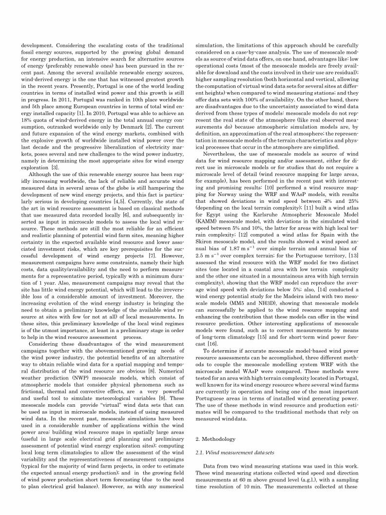
The AEP yield estimates and wind roses were computed consid-

ering the installation of one wind turbine (from the manufacturer

ENERCON, model E-82 with 2.0 MW of nominal power) in the same

location of site 1 (2), which coincide with the location of the wind

measuring station A (B). The power curve of this wind turbine is

depicted in Fig. 3.

2.5. Mesoscale–microscale coupling techniques

As previously mentioned, three different methodologies will be

tested for the coupling between mesoscale and microscale models,

which basically differ between themselves on the type of input

data supplied to microscale model.

2.5.1. Virtual wind measuring stations

The first methodology consists in taking from the simulated

wind data wind speed and direction time series, at the same points

(horizontal and vertical) where the measurements were made, and

use them as input to the microscale model. This allows a direct

comparison between simulated and measured wind, in terms of

Fig. 3. ENERCON’s E-82 wind turbine power curve.

x

its characteristics and resulting production estimates. Here, the

mesoscale model acts like ‘‘virtual wind measuring stations’’,

where wind speed and direction time series are computed for each

one of the two sites considered. These wind speed and direction

time series will be supplied to WAsP, which will build wind atlases

for the sites locations. The computation of the wind atlases consists

in removing and re-inserting the terrain effects on the wind data.

For this, a map that contains topography and ruggedness informa-

tion needs to be supplied to WAsP. This map consists of high reso-

lution (300, corresponding to approximately 90–100 m) information

of topography and ruggedness, making use of the Shuttle Radar

Topography Mission (SRTM) data, which obtained elevation data

on a near-global scale to generate the most complete high-resolu-

tion digital topographic database of the Earth [30]. Also supplied to

WAsP is the Corine Land Cover 2000 (CLC 2000) project data, which

consists of a vector map of the European environmental land-use

derived from satellite images [31], with a spatial resolution of

25 ha (approximately 500 500 m). It should be noted that this

methodology should not be considered as a real coupling between

the models, due to the fact that in this procedure WAsP is simply

fed with WRF wind output. This methodology was performed

mainly to compare the other two more refined coupling techniques

with the traditional results obtained when WAsP is simply fed with

WRF wind data, without any concern regarding other issues that

are important when coupling mesoscale and microscale models

(like topography data differences between the two models).

2.5.2. Wind atlas using WRF terrain data

The second methodology is similar to the first one, but intro-

duces an alternative way to build the wind atlas. The default ter-

rain data supplied to the WRF mesoscale model does not have

the same quality of the SRTM and CLC 2000, consisting of the GTO-

PO30 (for terrain elevation) and the U.S. Geological Survey (USGS,

for land-use information) data sets, made available by the USGS

with a horizontal grid resolution of 3000 of latitude/longitude

(approximately 900–1000 m). In addition to the improved resolu-

tion, the CLC2000 data set also has more land use categories than

the USGS one (44 instead of 24). Therefore, when WAsP removes

the terrain effects from the wind data computed by WRF, it will

consider its own high resolution terrain data and not the one used

by the WRF model in the wind data computation. This is what was

performed in Section 2.5.1. This discrepancy between types and

characteristics of terrain data can produce errors, because when

WAsP is removing the terrain effects, it is taking into account dif-

ferent terrain data than the one that is, in reality, included in the

wind data produced by WRF. In this methodology, the WRF model

the simulation domains (normally between 3 and 5 km), clearly

not enough to realistically represent the real terrain features. Con-

sequently, the wind simulated by the mesoscale model will have

deviations from the real wind due, in part, to this oversimplified

terrain representation. Microscale models offer a much more de-

tailed terrain data (topography and ruggedness) but, since micro-

scale models use the mesoscale output to downscale the local

wind characteristics, they will receive input wind data from the

mesoscale model that took into account terrain data with poor

resolution.

In order to extract from the mesoscale model winds that are

free (or the closest possible to being free) from the terrain influ-

ences, geostrophic winds extracted from the WRF simulations will

be used. By definition, the PBL is the lower part of the atmosphere

whose behavior is directly influenced by its contact with the plan-

etary surface, mainly due to effects of topography and ruggedness.

Above the PBL, the atmosphere is free of the planetary surface

influence and the wind is called geostrophic. To this end, the an-

nual mean PBL height was computed for the WRF simulated wind

data, taking into account WRF’s computation of the PBL height for

every time step of its simulations. The annual mean PBL height was

approximately 500 m, and the wind time series were extracted at

this height. This geostrophic wind (as it is free from the terrain

influences) is then used to build a wind atlas in WAsP. This result-

ing wind atlas computed by WAsP does not take into account any

information regarding topography and ruggedness, being that this

information is only used when WAsP downscales this wind atlas to

the site locations.

3. Results and discussion

3.1. Virtual wind stations

3.1.1. Comparison between the observed and simulated wind

The annual wind speed and direction time series for site 1 (2)

are taken from WRF and inserted in WAsP, as well as the wind

measurements from station A (B). The obtained results are pre-

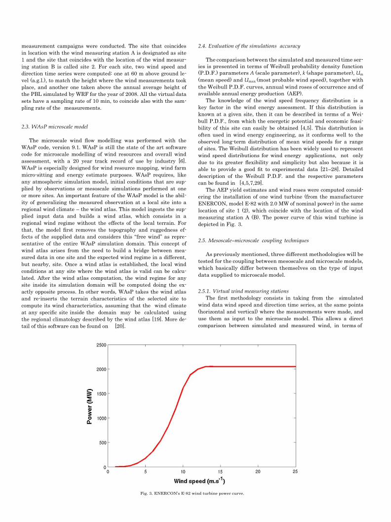
sented in Table 1 and Figs. 4–6.

In terms of the wind speed simulation, it is clear that using this

methodology the model significantly underestimates the wind

speed for both sites. The simulations foresee lower values for the

annual mean and most probable wind speed than those measured

by the respective wind measuring stations. The magnitude of the

Table 1

Comparison between Weibull parameters for measured and simulated wind data.

terrain data was transformed into a map readable by WAsP and the

wind atlases were built considering this terrain information. This

way, the wind atlases obtained from the WRF model will be prop-

erly computed. After this process, WAsP will re-insert the terrain

influences in the selected sites in order to compute the local wind

characteristics, but now using the high resolution terrain data.

Weibull

parameters

Site 1

(m s-1

)

Deviation to

measured data (%)

Site 2

(m s-1

)

Deviation to

measured data (%)

Using this methodology, WAsP will remove the WRF low resolu-

tion terrain effects from the simulated wind data, and then insert

high resolution terrain information leading to a finer scale topogra-

phy and surface ruggedness features that can have a large impact

on low-level wind fields.

2.5.3. Wind atlas using geostrophic wind

The third proposed approach aims to test the use of mesoscale

simulated winds that are not influenced by the local terrain. It is

widely accepted that one of the main limitations of mesoscale

models is their oversimplified representation of the real terrain

Virtual wind stations

A 6.20 -22.5 6.40 -36.0

k 2.54 -5.6 2.57 2.4

Um 5.52 -22.0 5.66 -36.3

Umax 5.09 -24.4 5.28 -35.3

WRF terrain data

A 8.60 7.5 10.40 4.0

k 2.53 -5.9 2.47 -1.6

Um 7.60 7.3 9.26 4.3

Umax 7.05 4.7 8.43 3.2

Geostrophic wind

A 7.10 -11.3 8.50 -15.0

(topography, ruggedness, etc.), due to insufficient detail of the ter- k 3.20 19.0 3.05 21.5

rain data supplied to the model (as stated above, typically around Um 6.38 -9.9 7.59 -14.5

3000 of resolution) and also due to the resolution typically used in Umax 6.32 -6.2 7.46 -8.6

Measured A 8.00 – 10.00 –

k 2.69 – 2.51 –

Um 7.08 – 8.88 –

Umax 6.73 – 8.17 –

Fig. 4. Weibull P.D.F. curves for measured and simulated wind.

differences is similar in the results for the Weibull scale parameter

A, but for the shape parameter k the model behavior is quite rea-

sonable. Comparing both sites, it is clear that the model presents

a worse overall performance in site 2.

Fig. 4 clearly reflects the strong wind speed underestimation by

the model in both sites. The simulated Weibull curves present a vis-

ible shifting to the left side of the wind speed axis, meaning that the

model foresees higher frequencies of low wind speeds and, by con-

sequence, lower frequencies of strong wind speeds than in reality.

Also, it is visible that the model considers wind speeds around 5–

6 m s-1 as the most frequent ones, while observations show that,

in reality, the most frequent wind speeds are around 7–8 m s-1,

which is in accordance with the most probable wind speeds values

presented in Table 1. Again, the discrepancy between simulated and

observed Weibull functions is higher for site 2.

In terms of the wind direction simulation, Fig. 5 presents the an-

nual occurrence wind roses using simulated and measured data for

site 1 and Fig. 6 for site 2. In terms of occurrences on site 1, the ob-

served and simulated occurrence wind roses are quite similar. The

model is able to successfully determine the dominant sector, and

to reasonably simulate the relative percentage of occurrences of

the remaining sectors. In site 2 the results are somewhat worse,

as the model considers the north–northwest sector as the most

dominant while the observations show that it is the northwest sec-

tor that has the highest percentage of occurrences. The distribution

of the occurrence frequencies of all sectors in this site appears to be

rotated about 25° clockwise. It is also visible in all the computed

results that, while measurements show that the sites have a

slightly different wind regime, the model considers both sites with

similar wind circulation patterns.

3.1.2. Comparison of the observed and simulated production estimates

The resulting values in terms of AEP and AEP wind roses are pre-

sented in Table 2 and Figs. 7 and 8. Looking at Table 2, and as expected,

the wind speed underestimation by the WRF model is strongly re-

flected in the production estimates. Using the simulated wind data

as input in WAsP, the production estimates are clearly lower than

those that are based in observed wind data. Again, the model presents

poorer performance for site 2, which is expected due to the worst sim-

ulation of the wind speed distribution in this site.

The influence of the wind speed underestimation on the AEP

estimates is better explained when the Weibull curves (presented

in Fig. 4) are analyzed together with the power curve of the wind

turbine here considered. As can be seen in Fig. 3, the cut-in speed

(minimum wind speed at which the wind turbine will generate

usable power) for this wind turbine is approximately 2 m s-1. As

shown in Table 1, the simulated average wind speeds for both sites

are significantly lower, which will induce lower production esti-

mates. Moreover, Fig. 4 shows that the simulations foresee higher

frequencies of wind speeds below 2 m s-1 than what was observed.

AEP estimates are significantly underestimated due to the predic-

tion of higher frequencies of low wind speeds (part of them below

the cut-in speed of the wind turbine that will originate null energy

productions) together with lower frequencies of strong winds

(which would originate high energy productions).

Fig. 7 shows the AEP wind roses for site 1 and Fig. 8 for site 2. The

observed and simulated AEP wind roses for site 1 are quite similar,

with the model able to successfully determine the dominant sector

and the relative percentage of AEP of the remaining sectors. Again,

for site 2 the results are somewhat worse, as the model considers

the north–northwest sector as the most dominant while the obser-

vations show that it is the northwest sector that has the highest

percentage of AEP. The distribution of the occurrence frequencies

of all sectors in this site appears to be rotated about 25° clockwise.

In this methodology it becomes clear that the model main error

source is the wind speed underestimation, which is mainly due to

the weak terrain representation by the mesoscale model. The

mesoscale model represents the terrain in its simulation grid

smoother and with a systematic lower topography than in reality

and these two factors will produce a wind speed underestimation

in its output. On the one hand, it is known that areas with lower

altitude are, in general, characterized by lower wind speeds. In fact,

the WRF model considers site 1 with 25% lower altitude than in

reality, while site 2 is depicted in WRF simulation domain with less

than 50% of its real altitude. Consequently, if the model sees the

simulation point with lower altitude than in reality, the simulated

wind speeds for the considered site will be lower than what was

measured. On the other hand, mountainous areas frequently give

origin to wind speed-up effects. The wind flow suffers a compres-

sion on the windy side of the mountain as the flow moves to the

mountain top, followed by an expansion when the air masses pass

the mountain ridge and flow to the lee side of the mountain, due to

its decompression. Ultimately, if the model represents the terrain

as being smoother and the simulation point as being lower than

in reality, these speed-up effects will be attenuated, originating

an underestimation of the wind speeds.

The combination of these factors, which arise as a consequence

of the distorted terrain representation by the mesoscale model, will

induce lower simulated wind speeds. As an addition to these fac-

tors, the characteristics of the real local topography can also gener-

ate physical gradients (thermal, pressure) due to the presence or

absence of close mountains that will also contribute to errors in

the wind speed simulation by the mesoscale model, which is not

able to represent these real topography characteristics.

Fig. 5. Occurrences wind roses for site 1 ((a): measured; (b): virtual wind measuring station methodology; (c): WRF terrain data coupling technique; (d): geostrophic wind

coupling technique).

Furthermore, results are clearly worse for site 2 showing that the

surrounding terrain complexity plays an important role in the wind

speed simulation. In this site, located in a more complex terrain

than site 1 (as showed in Fig. 1b, with the RIX values for both sites),

the limitations of the mesoscale model are more exposed since the

mesoscale model representation of the local topography is more

distorted.

3.2. Wind atlas using WRF terrain data

3.2.1. Comparison of the observed and simulated wind main

characteristics

The results in terms of the Weibull distribution parameters A, k,

and Um and Umax, Weibull P.D.F. curves and annual occurrence

wind roses are presented in Table 1 and Figs. 4–6.

The model performance is clearly improved when this coupling

technique is used. According to Table 1, the wind speed is now

slightly overestimated, with deviations of 7.3% for site 1 and 4.3%

for site 2 in terms of mean wind speed, and of 4.7% for site 1 and

3.2% for site 2 in terms of most probable wind speed. The magni-

tude of the differences is similar for the Weibull scale parameter

A and the shape parameter k, with the latter being underestimated.

Comparing both sites, now the models present a slightly better

overall performance for site 2.

As for the Weibull P.D.F. curves of the observed and simulated

wind for both sites depicted in Fig. 4, results clearly show an

improvement of the model performance when using this tech-

nique, with simulated Weibull curves much closer to the ob-

served ones. An inverse behavior of the models is now visible,

since the wind speeds are slightly overestimated for both sites.

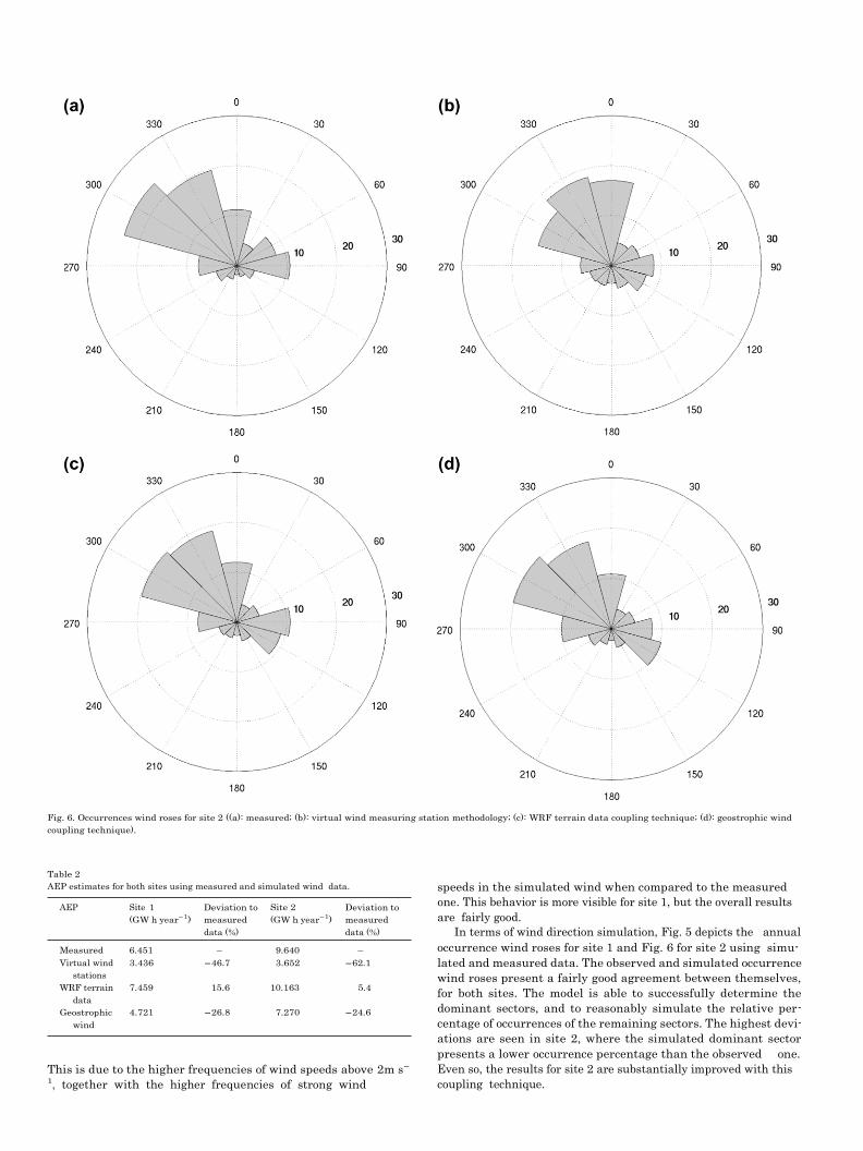
Fig. 6. Occurrences wind roses for site 2 ((a): measured; (b): virtual wind measuring station methodology; (c): WRF terrain data coupling technique; (d): geostrophic wind

coupling technique).

Table 2

AEP estimates for both sites using measured and simulated wind data.

speeds in the simulated wind when compared to the measured

AEP Site 1

(GW h year-1

)

Deviation to

measured

data (%)

Site 2

(GW h year-1

)

Deviation to

measured

data (%)

one. This behavior is more visible for site 1, but the overall results

are fairly good.

In terms of wind direction simulation, Fig. 5 depicts the annual

Measured 6.451 – 9.640 – occurrence wind roses for site 1 and Fig. 6 for site 2 using simu-

Virtual wind

stations

WRF terrain

data

Geostrophic

wind

3.436 -46.7 3.652 -62.1

7.459 15.6 10.163 5.4

4.721 -26.8 7.270 -24.6

lated and measured data. The observed and simulated occurrence

wind roses present a fairly good agreement between themselves,

for both sites. The model is able to successfully determine the

dominant sectors, and to reasonably simulate the relative per-

centage of occurrences of the remaining sectors. The highest devi-

ations are seen in site 2, where the simulated dominant sector

presents a lower occurrence percentage than the observed one.

This is due to the higher frequencies of wind speeds above 2m s-

1, together with the higher frequencies of strong wind

Even so, the results for site 2 are substantially improved with this

coupling technique.

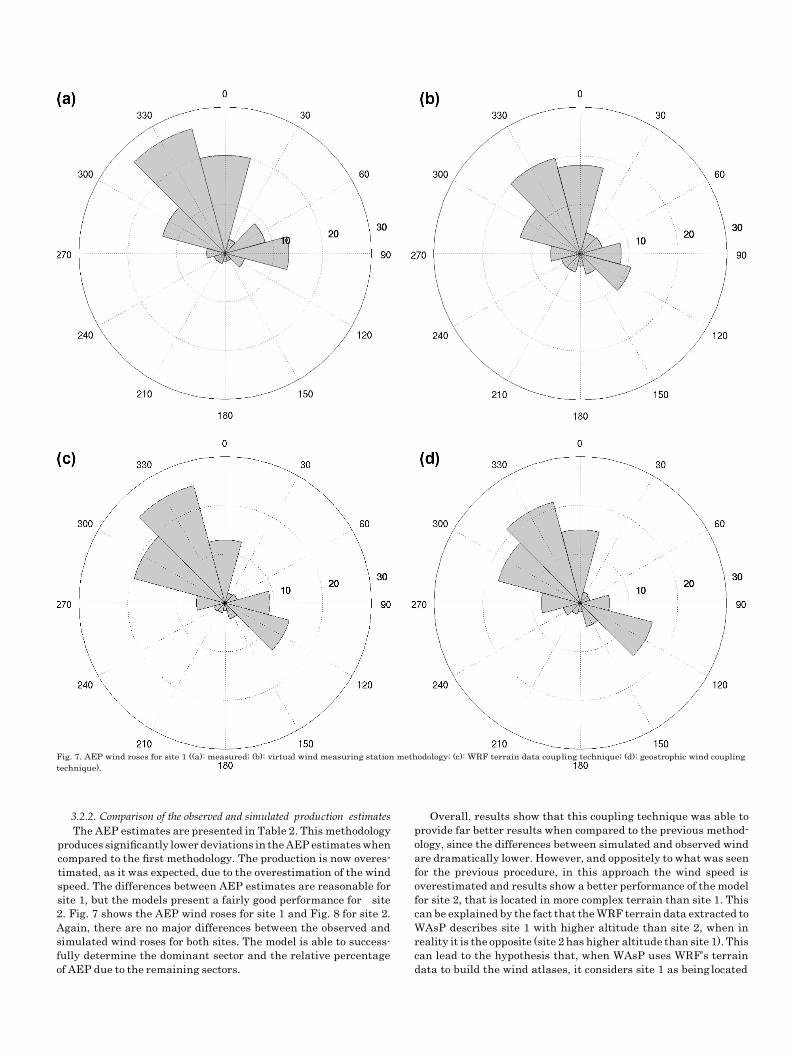
Fig. 7. AEP wind roses for site 1 ((a): measured; (b): virtual wind measuring station methodology; (c): WRF terrain data coupling technique; (d): geostrophic wind coupling

technique).

3.2.2. Comparison of the observed and simulated production estimates

The AEP estimates are presented in Table 2. This methodology

produces significantly lower deviations in the AEP estimates when

compared to the first methodology. The production is now overes-

timated, as it was expected, due to the overestimation of the wind

speed. The differences between AEP estimates are reasonable for

site 1, but the models present a fairly good performance for site

2. Fig. 7 shows the AEP wind roses for site 1 and Fig. 8 for site 2.

Again, there are no major differences between the observed and

simulated wind roses for both sites. The model is able to success-

fully determine the dominant sector and the relative percentage

of AEP due to the remaining sectors.

Overall, results show that this coupling technique was able to

provide far better results when compared to the previous method-

ology, since the differences between simulated and observed wind

are dramatically lower. However, and oppositely to what was seen

for the previous procedure, in this approach the wind speed is

overestimated and results show a better performance of the model

for site 2, that is located in more complex terrain than site 1. This

can be explained by the fact that the WRF terrain data extracted to

WAsP describes site 1 with higher altitude than site 2, when in

reality it is the opposite (site 2 has higher altitude than site 1). This

can lead to the hypothesis that, when WAsP uses WRF’s terrain

data to build the wind atlases, it considers site 1 as being located

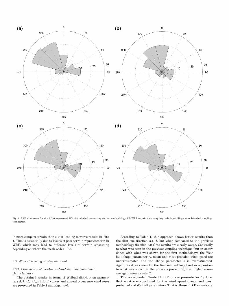
Fig. 8. AEP wind roses for site 2 ((a): measured; (b): virtual wind measuring station methodology; (c): WRF terrain data coupling technique; (d): geostrophic wind coupling

technique).

in more complex terrain than site 2, leading to worse results in site

1. This is essentially due to issues of poor terrain representation in

WRF, which may lead to different levels of terrain smoothing

depending on where the mesh nodes lie.

3.3. Wind atlas using geostrophic wind

3.3.1. Comparison of the observed and simulated wind main

characteristics

The obtained results in terms of Weibull distribution parame-

ters A, k, Um, Umax, P.D.F. curves and annual occurrence wind roses

are presented in Table 1 and Figs. 4–6.

According to Table 1, this approach shows better results than

the first one (Section 3.1.1), but when compared to the previous

methodology (Section 3.2.1) its results are clearly worse. Contrarily

to what was seen in the previous coupling technique (but in accor-

dance with what was shown for the first methodology), the Wei-

bull shape parameter A, mean and most probable wind speed are

underestimated and the shape parameter k is overestimated.

Again, as it was seen for the first methodology (and in opposition

to what was shown in the previous procedure), the higher errors

are again seen for site 2.

The correspondent Weibull P.D.F. curves, presented in Fig. 4, re-

flect what was concluded for the wind speed (mean and most

probable) and Weibull parameters. That is, these P.D.F. curves are

similar to the ones regarding the first approach, with a clear shift-

ing to the left of the curves that distorts the real wind speed distri-

bution and will originate the underestimation of the wind speed.

As for the annual occurrence wind roses for both sites using simu-

lated and measured data (Figs. 5 and 6), the model is able to rea-

sonably simulate the dominant sectors. Moreover, a

standardization of the local wind regimes is clear, when they

should be more distinct.

3.3.2. Comparison of the observed and simulated production estimates

The AEP estimates are presented in Table 2. As a consequence of

the results of this approach for the wind speed and Weibull param-

eters, this coupling technique clearly produces a strong underesti-

mation of the AEP estimates. Again, the estimates deviation are

higher when compared to the previous methodology and lower rel-

atively to the previous one. For site 1 an AEP underestimation of

26.8% is obtained and for site 2 an underestimation of 24.6% is

computed.

The AEP wind roses, depicted in Figs. 7 and 8, show that for site 1

they are fairly similar, but for site 2 higher discrepancies are de-

tected. Overall results of this approach show that this coupling

technique was not able to improve the simulations accuracy, at

least when it is compared to the previous one. Although an

improvement was detected relatively to the first methodology,

the use of a geostrophic approach to overcome terrain effects influ-

ence on the simulations is not enough to obtain reliable and realis-

tic results.

4. Conclusions

This work was undertaken with the main objective of testing

the performance of three mesoscale–microscale coupling tech-

niques for the wind (speed and direction) and AEP simulation esti-

mates, when compared to the same estimates based in measured

wind data. For this purpose, the mesoscale model WRF and the

microscale model WAsP were used. Simulations were performed

in the exact same locations were wind measurement campaigns

were conducted, allowing the comparison between simulated

and observed wind data in terms of atmospheric flow characteris-

tics and production estimates. The sites differ in terms of local ter-

rain complexity in order to analyze the sensitivity of the

methodologies performance to these terrain characteristics, which

is seen as one of the main sources of error in the near surface winds

simulation due to the mesoscale model low resolution terrain data.

The obtained results show that, if the mesoscale output is di-

rectly inserted in the microscale model (first approach), the local

wind speed distributions are severely misrepresented leading to

a strong underestimation of the wind speed and, consequently, of

the estimated AEP. These deviations between simulated and mea-

sured data are most likely due to the mesoscale model misrepre-

sentation of the local terrain characteristics together with the

discrepancies between the terrain effects induced by the mesoscale

model and the terrain effects removed by the microscale model

when the wind atlases are computed by it. Moreover, this method-

ology proved that the local terrain complexity is an important fac-

tor in the near-surface wind simulation, since worse results were

seen for the site located in more complex surrounding terrain.

The second approach, which is an attempt to correct the above-

mentioned terrain data discrepancies between the mesoscale and

microscale model, shows significant improvements in all the results

leading to more reasonable values. This coupling technique proves

the importance of, when introducing mesoscale-derived wind data

in the microscale model, the mesoscale terrain data should be con-

sidered. By doing this, the distorted mesoscale-induced terrain ef-

fects are successfully removed and, after the subsequent inclusion

of high resolution terrain effects, the simulations and AEP estimates

become significantly closer to the observed wind data.

The third tested procedure arises as an attempt to completely

disregard the mesoscale terrain data in the wind simulation, using

geostrophic winds in the wind atlases computation. The obtained

results show significant improvement when compared to the first

methodology, but presented far worse performance in comparison

to the second approach. Therefore, and taking into account the re-

sults presented in this study, it is advised to follow the second

methodology in order to obtain the most reliable and accurate

wind simulations.

Considering these results, it is clear that the quality and accu-

racy of the models terrain representation (mainly on the mesoscale

model, since the microscale model already has terrain data of good

quality) is a key factor in near-surface wind simulation, together

with the local surrounding terrain complexity. The microscale

model WAsP is of linear type and the terrain complexity can induce

this model to work outside of its envelope, and if its input data

comes already with deviations this limitation of WAsP will be

amplified. Both sites are located in a mountainous area, and the lo-

cal terrain complexity indicates that the application of these (or

others) methodologies must be handled with care, since they were

obtained solely with numerical simulation models and, therefore,

have a considerable degree of uncertainty. Nevertheless, the sec-

ond methodology presented here showed considerably good re-

sults, with a clear improvement of the models performance when

compared to the other approaches.

Although encouraging results were obtained, they indicate that

the use of mesoscale–microscale models for wind resource assess-

ment purposes cannot still be seen as a substitute to locally ac-

quired wind data for specific wind farm projects, since several

sub-grid features are not well represented by the existing parame-

terizations and terrain data. Nevertheless, it is important to assert

that mesoscale–microscale modelling results can be an important

factor in initial studies, especially in sites where the terrain is

somewhat smooth, or as a tool for preliminary wind resource map-

ping and assessments.

References

[1] Global Wind Energy Council. Global Wind Report, Annual market update.

<http://www.gwec.net/fileadmin/documents/NewsDocuments/

Annual_report_2011_lowres.pdf>; 2011.

[2] Global Wind Energy Council. Global Wind Energy Report. <http://

www.gwec.net/fileadmin/images/Publications/

GWEC_annual_market_update_2010_-_2nd_edition_April_2011.pdf>; 2010.

[3] Purvins A, Zubaryeva A, Llorente M, Tzimas E, Mercier A. Challenges and

options for a large wind power uptake by the European electricity system. Appl

Energy 2011;88(5):1461–9.

[4] Ucar A, Balo F. Investigation of wind characteristics and assessment of wind-

generation potentiality in Uludag-Bursa, Turkey. Appl Energy

2009;86(3):333–9.

[5] Ucar A, Balo F. Evaluation of wind energy potential and electricity generation

at six locations in Turkey. Appl Energy 2009;86(10):1864–72.

[6] Soares A, Pinto P, Pilão R. Mesoscale modelling for wind resource evaluation

purposes: a test case in complex terrain. In: International conference on

renewable energies and power quality. <http://www.icrepq.com/icrepq’10/

433-Soares.pdf>; 2010.

[7] Kwon S-D. Uncertainty analysis of wind energy potential assessment. Appl

Energy 2010;87(3):856–65.

[8] Beccali M, Cirrincione G, Marvuglia A, Serporta C. Estimation of wind velocity

over a complex terrain using the generalized mapping regressor. Appl Energy

2010;87(3):884–93.

[9] Carvalho D, Rocha A, Gómez-Gesteira M, Santos C. A sensitivity study of the

WRF model in wind simulation for an area of high wind energy. Environ Model

Softw 2012;33:23–34.

[10] Byrkjedal O, Berge E. The Use of WRF for wind resource mapping in Norway.

In: 9th WRF users’ workshop; 2008.

[11] Mortensen NG, Hansen JC, Badger J, Jørgensen H, Hasager CB, Paulsen US, et al.

Wind atlas for Egypt: measurements, micro- and mesoscale modelling. In:

European wind energy conference (EWEC); 2006.

[12] Gastion M, Pascal E, Frias L, Marti I, Irigoyen U, Cantero E, et al. Wind resources

map of Spain at mesoscale: methodology and validation. In: European wind

energy conference (EWEC); 2008.

[13] Chagas G, Guedes RA, Manso MDO. Estimating wind resource using mesoscale

modelling. In: European wind energy conference (EWEC); 2009.

[14] Miranda P, Valente M, Ferreira J. Simulação numérica do escoamento

atmosférico sobre a Ilha da Madeira: efeitos não lineares e de estratificação

no estabelecimento do potencial eólico na zona do paul da Serra. Technical

Report of the Lisbon University Geophysical Centre; 2003.

[15] Cameron WP, Lew D, McCaa J, Cheng S, Eichelberger S, Grimit E. Creating the

dataset for the western wind and solar integration study (USA). Wind Eng

2008;32:325–38.

[16] Cassola F, Burlando M. Wind speed and wind energy forecast through Kalman

filtering of numerical weather prediction model output. Appl Energy

2012;99:154–66.

[17] Bowen AJ, Mortensen NG. Exploring the limits of WAsP: the wind atlas

analysis and application program. In: Proceedings of the European union wind

energy conference; 1996. p. 584–7.

[18] Skamarock WC, Klemp JB, Dudhia J, Gill DO, Barker DM, Huang XY, et al. A

description of the advanced research WRF Version 3. NCAR Technical Note,

Mesoscale and Microscale Meteorology Division of NCAR; 2008.

[19] Troen I, Petersen EL. European wind atlas. Risø National Laboratory, Technical

University of Denmark; 1989.

[20] Mortensen NG, Heathfield DN, Myllerup L, Landberg L, Rathmann O. Wind

atlas analysis and application program, WAsP 9 Help Facility. Risø National

Laboratory, Technical University of Denmark; 2007.

[21] Corotis RB, Sigl AB, Klein J. Probability models of wind velocity magnitude and

persistence. Sol Energy 1978;20:481–93.

[22] Garcia A, Torres JL, Prieto E, De Francisco A. Fitting wind speed distributions: a

case study. Sol Energy 1998;62:139–44.

[23] Gupta BK. Weibull parameters for annual and monthly wind speed

distributions for five locations in India. Sol Energy 1986;37:469–71.

[24] Hennessey Jr JP. A comparison of the Weibull and Rayleigh distributions for

estimating wind power potential. Wind Eng 1978;2(3):156–64.

[25] Justus CG, Hargraves WR, Mikhail A, Graber D. Methods for estimating wind

speed frequency distributions. J Appl Meteorol 1978;17(3):350–3.

[26] Rehman S, Halawani TO, Husain T. Weibull parameters for wind speed

distribution in Saudi Arabia. Sol Energy 1994;53(6):473–9.

[27] Stevens MJM, Smulders PT. The estimation of the parameters of the Weibull

wind speed distribution for wind energy utilization purposes. Wind Eng

1979;3(2):132–45.

[28] Takle ES, Brown JM. Note on the use of Weibull statistics to characterize wind-

speed data. J Appl Meteorol 1991;30:823–33.

[29] Akpinar EK, Akpinar S. An assessment on seasonal analysis of wind energy

characteristics and wind turbine characteristics. Energy Convers Manage

2005;46(11–12):1848–67.

[30] Farr TG, Rosen PA, Caro E, Crippen R, Duren R, Hensley S, et al. The shuttle

radar topography mission. Rev Geophys 2007;45(2):1–33.

[31] Büttner G, Feranec J, Jaffrain G, Mari L, Maucha G, Soukup T. The CORINE land

cover project. In: Reuter R, editor. EARSeL eProceedings, Paris; 2004. p. 331–

46.