Master of Science Thesis

KTH School of Industrial Engineering and Management

Energy Technology EGI-2012-78MSC

Division of Heat and Power Technology

SE-100 44 STOCKHOLM

Reliability of wind farm design tools

in complex terrain

A comparative study of commercial software

Tobias Timander

Jimmy Westerlund

i

Master of Science Thesis EGI 2012: 78MSC

Reliability of wind farm design tools in

complex terrain - A comparative study of

commercial software

Tobias Timander

Jimmy Westerlund

Approved

2012-10-04

Examiner

Joachim Claesson

Supervisor

Stefan Ivanell

Commissioner

Contact person

Abstract

A comparative study of two different approaches in wind energy simulations has been made where the

aim was to investigate the performance of two commercially available tools. The study includes the linear

model by WAsP and the computational fluid dynamic model of WindSim (also featuring an additional

forest module). The case studied is a small wind farm located in the inland of Sweden featuring a fairly

complex and forested terrain. The results showed similar estimations from both tools and in some cases

an advantage for WindSim. The site terrain is however deemed not complex enough to manifest the

potential benefits of using the CFD model. It can be concluded that estimating the energy output in this

kind of terrain is done satisfyingly with both tools. WindSim does however show a significant

improvement in consistency when estimating the energy output from different measurement heights when

using the forest module compared to only using the standardized roughness length.

Keywords: WindPRO, WAsP, WindSim, Wind Energy, Wake, Complex Terrain, Forest, CFD, Linear

Model.

ii

Table of Contents

Abstract ............................................................................................................................................................................ i

Index of figures .............................................................................................................................................................. v

Index of tables .............................................................................................................................................................. vi

Symbols ......................................................................................................................................................................... vii

Abbreviations ................................................................................................................................................................ ix

Acknowledgements ...................................................................................................................................................... ix

1 Introduction .......................................................................................................................................................... 1

1.1 Aims and Objectives ................................................................................................................................... 1

1.2 Limitations ................................................................................................................................................... 1

2 Wind power fundamentals .................................................................................................................................. 2

2.1 Wind energy ................................................................................................................................................. 2

2.1.1 Roughness and wind shear ............................................................................................................... 2

2.1.2 Displacement height .......................................................................................................................... 4

2.1.3 Orography ........................................................................................................................................... 5

2.1.4 Obstacles ............................................................................................................................................. 5

2.1.5 Power in the wind .............................................................................................................................. 5

2.1.6 Turbulence .......................................................................................................................................... 7

2.1.7 Wake effect ......................................................................................................................................... 7

2.1.8 Statistics for wind energy applications ............................................................................................ 9

3 Wind measurement ............................................................................................................................................12

3.1 Anemometers .............................................................................................................................................12

3.1.1 Cup anemometers ............................................................................................................................12

3.1.2 Pressure plate anemometers ...........................................................................................................13

3.1.3 Ultrasonic anemometers .................................................................................................................13

3.1.4 Peripherals and anemometer measurement quality ....................................................................13

3.2 Wind direction measurements and charts .............................................................................................14

3.3 SODAR ......................................................................................................................................................15

4 Atmospheric science ..........................................................................................................................................17

4.1 Temperatures .............................................................................................................................................17

4.2 Atmospheric stability ................................................................................................................................17

4.3 Obukhov length ........................................................................................................................................18

5 Computational fluid dynamics .........................................................................................................................20

5.1 Pre-processor .............................................................................................................................................20

5.2 Solver and the finite volume method .....................................................................................................20

iii

5.3 Post-processor ...........................................................................................................................................21

5.4 The Governing equations of the flow of a compressible Newtonian fluid .....................................21

5.5 Governing equations for turbulent compressible flows: The Reynolds-averaged Navier-Stokes

equations ..................................................................................................................................................................23

5.6 Turbulence and its modeling ...................................................................................................................24

5.6.1 The k-ε model ...................................................................................................................................25

6 Commercial software for wind farm layout optimization ...........................................................................27

6.1 WAsP ..........................................................................................................................................................27

6.2 WindPRO ...................................................................................................................................................27

6.2.1 METEO ............................................................................................................................................28

6.2.2 MODEL ............................................................................................................................................28

6.2.3 MCP ...................................................................................................................................................28

6.2.4 PARK .................................................................................................................................................28

6.2.5 LOSS ..................................................................................................................................................29

6.2.6 OPTIMIZE ......................................................................................................................................29

6.3 WindSim .....................................................................................................................................................29

6.3.1 Accuracy ............................................................................................................................................29

6.3.2 Input data ..........................................................................................................................................30

6.3.3 Using WindSim.................................................................................................................................30

7 Methodology .......................................................................................................................................................35

7.1 Using the simulation tools .......................................................................................................................35

7.1.1 Terrain properties ............................................................................................................................35

7.1.2 General parameters ..........................................................................................................................39

7.1.3 WindSim settings and convergence ..............................................................................................40

7.2 Treating the measured data .....................................................................................................................43

7.2.1 Actual electricity production and correction ...............................................................................47

7.3 Simulation cases.........................................................................................................................................49

7.3.1 Simulation cases 2008/2009 ...........................................................................................................50

7.3.2 Simulation cases 2011 ......................................................................................................................54

8 Results ..................................................................................................................................................................56

8.1 2008/2009 ..................................................................................................................................................56

8.1.1 Standard cases ...................................................................................................................................56

8.1.2 Wake models .....................................................................................................................................56

8.1.3 Roughness height .............................................................................................................................59

8.1.4 Forest module ...................................................................................................................................59

8.1.5 Displacement height ........................................................................................................................61

iv

8.1.6 Measuring height dependence ........................................................................................................61

8.2 2011 .............................................................................................................................................................63

9 Discussion ...........................................................................................................................................................64

9.1 The wind data ............................................................................................................................................64

9.2 Correcting the actual generation .............................................................................................................64

9.3 About the terrain .......................................................................................................................................64

9.4 2008/2009 Simulations ............................................................................................................................65

9.4.1 The standard cases 2008/2009 ......................................................................................................65

9.4.2 Wake models .....................................................................................................................................65

9.4.3 Forest module ...................................................................................................................................65

9.4.4 Roughness height .............................................................................................................................65

9.4.5 Displacement height ........................................................................................................................66

9.4.6 Measuring height dependence ........................................................................................................66

9.5 2011 Simulations .......................................................................................................................................66

10 Conclusions .........................................................................................................................................................67

11 Future work .........................................................................................................................................................69

12 Bibliography .......................................................................................................................................................70

Appendices ...................................................................................................................................................................74

v

Index of figures

Figure 2.1: Wind profile in forest (Hui & Crockford, u.d.) .................................................................................... 4

Figure 2.2: The frequency distribution for a fictive site. .......................................................................................10

Figure 2.3: The probability distribution of the wind speed at an imaginary site. ..............................................11

Figure 2.4: The cumulative probability of the wind speed at an imaginary site. ...............................................11

Figure 3.1: Left: A cup anemometer (Direct Industry, 2012a). Center: An ultrasonic anemometer (Direct

Industry, 2012b). Right: A cup anemometer with a wind vane (ENVCO, 2012) .............................................13

Figure 3.2: A wind rose generated by WindSim. ....................................................................................................15

Figure 3.3: AQ 500 SODAR device. ........................................................................................................................15

Figure 5.1: The principle of conservation of the general flow variable in a finite control volume. ...........21

Figure 7.1: Timeline of the available data. ...............................................................................................................35

Figure 7.2: An orographic map of the terrain created in WindPRO with a resolution of 18 m. ....................36

Figure 7.3: Detailed orographic map of the terrain in Site A created in WindPRO with a resolution of 6 m.

........................................................................................................................................................................................37

Figure 7.4: The layout of the wind turbines and the placement of the wind measurements. .........................39

Figure 7.5: The refined grid generated in WindSim. ..............................................................................................40

Figure 7.6: Convergence of the spot values in WindSim. Convergence was achieved after around 80

iterations (top) to 150 iterations (bottom). ..............................................................................................................41

Figure 7.7: The residual values in WindSim. An acceptable level was achieved after around 160 iterations

(top) to 180 iterations (bottom). ...............................................................................................................................42

Figure 7.8: The park layout in WindSim seen from northeast. ............................................................................42

Figure 7.9: Energy roses placed on the location of the SODAR device in 2011. .............................................45

Figure 7.10: Energy content in the wind for Sweden during 1991-2011 (Carlstedt, 2012). ............................47

Figure 7.11: A map of the terrain for Site A, the circle marks the site (Hitta.se, 2012). ..................................48

Figure 7.12: A map of the terrain for Site B, the circle marks the site (Hitta.se, 2012). ..................................49

Figure 7.13: Timeline for simulation cases 2008/2009. ........................................................................................50

Figure 7.14: The forest canopy generated by WindSim and the underlying roughness height [m] ranging

from white (0.0002) to red (0.4). ...............................................................................................................................54

Figure 7.15: Timeline for simulation cases 2011. ...................................................................................................55

Figure 8.1: Results from wake model cases for 2008/2009 presented as the percentage difference from the

actual generation of the individual turbines. ...........................................................................................................57

Figure 8.2: Wake model results for WindSim standard case FM (Jensen). .............................................................58

Figure 8.3: Wake model results for WindSim wake model case 1 (Larsen)..............................................................58

Figure 8.4: Wake model results for WindSim wake model case 2 (Ishihara, Yamaguchi, Fujino). ......................59

Figure 8.5: The wind speed profile at VKV1 – Ellen (sector 0). .........................................................................60

Figure 8.6: Results from varying the measuring height. ........................................................................................62

Figure 8.7: Results from the forest module cases for all measurement heights. ...............................................63

vi

Index of tables

Table 2.1: Roughness lengths for different types of terrain (Manwell, et al., 2002) (Nelson, 2009). ............... 3

Table 2.2: Roughness classification according to the European Wind Atlas (EMD International A/S,

2010). ............................................................................................................................................................................... 3

Table 5.1: Equations governing the flow of a Newtonian compressible fluid (Versteeg & Malalasekera,

2007). .............................................................................................................................................................................22

Table 5.2: Governing equations for turbulent compressible flows (Versteeg & Malalasekera, 2007). ..........24

Table 5.3: Common RANS turbulence models (Versteeg & Malalasekera, 2007). ...........................................25

Table 5.4: The k-ε model equations (Versteeg & Malalasekera, 2007). .............................................................26

Table 7.1: Availability of the wind measurements from the SODAR device. ...................................................44

Table 7.2: Comparison of the mean wind speed [m/s] for all wind directions between 2008/2009 and

2011. ..............................................................................................................................................................................46

Table 7.3: Detailed operation information for Dalarna county from 2006 to 2011 (Carlstedt, 2012). .........48

Table 7.4: Generated electricity in MWh for Site B and the correction factor. ................................................49

Table 7.5: Generated electricity in MWh for Site A during 2011 and May-July. ...............................................49

Table 7.6: The roughness lengths z0, in meter, used to classify the terrain in the standard cases. .................51

Table 7.7: Detailed description of the WindSim forest module configuration. ................................................51

Table 7.8: Description of the wake model settings in the WindPRO wake model cases. ...............................52

Table 7.9: Description of the wake model settings in the WindSim wake model cases. .................................52

Table 7.10. Roughness heights used for the WindPRO and WindSim roughness height cases. ....................53

Table 7.11: Forest module simulation settings in WindSim. ................................................................................53

Table 7.12: Displacement height cases tested in WindPRO. ...............................................................................54

Table 8.1: Results from standard cases for 2008/2009 and the actual production in MWh...........................56

Table 8.2: Results from wake model cases for 2008/2009 in MWh as well as losses. .....................................57

Table 8.3: Results from roughness height cases for 2008/2009 in MWh. .........................................................59

Table 8.4: Results from forest module cases for 2008/2009 in MWh. ...............................................................60

Table 8.5: Results from displacement height cases for 2008/2009 in MWh. ....................................................61

Table 8.6: Results from cases for 2011 in MWh. ...................................................................................................63

vii

Symbols

Symbol Unit Description

By rotor swept area

Cup anemometer area exposed to the wind

Forest resistive force constant (force proportional to velocity)

Forest resistive force constant (force proportional to velocity squared)

The drag coefficient

Power coefficient

The specific heat capacity

Kinetic energy

Drag force

Gravitational acceleration

Height at which wind speed equals

Height at which wind speed equals

Energy

Turbulence intensity

Mean kinetic energy

Turbulent kinetic energy

Instantaneous turbulent kinetic energy

von Kármán constant

The Obukhov length

Mass

Wind turbine power output

Power in the wind

Pressure

A standard reference pressure (1 bar)

The individual gas constant

Rotor radius

Mixing ratio of air and water vapor

Forest resistive force (proportional to the wind velocity)

Forest resistive force (proportional to the wind velocity squared)

Source term (energy) for a Newtonian compressible fluid

Source term (x-momentum) for a Newtonian compressible fluid

Source term (y-momentum) for a Newtonian compressible fluid

viii

Source term (z-momentum) for a Newtonian compressible fluid

Source term (general transport eq.) for a Newtonian compressible fluid

Temperature in Kelvin

Virtual temperature in Kelvin

Time

U Mean velocity vector

Mean velocity component in the x-direction

Instantaneous velocity component in the x-direction

Fluctuating velocity component in the x-direction

Velocity at meters behind the rotor due to wake effects

Friction velocity

V Mean velocity component in the y-direction

Instantaneous velocity component in the y-direction

Fluctuating velocity component in the y-direction

Wind speed

Measured wind speed at height

Mean velocity component in the z-direction

Instantaneous velocity component in the z-direction

Fluctuating velocity component in the z-direction

X coordinate

Downstream distance from rotor

Y coordinate

Height above ground or z coordinate

Roughness length

A general flow variable

Wind shear exponent (power law)

Stability function constant at stable atmosphere

Diffusion coefficient

Stability function constant at unstable atmosphere

The Kronecker delta

Ratio of the gas constants for air and water vapor

Turbulent kinetic energy dissipation rate

The dimensionless Obukhov length

Weibull shape factor

Potential temperature

ix

Virtual potential temperature

Weibull scale factor

Dynamic viscosity for volumetric deformations

Dynamic viscosity for linear deformations

Turbulent dynamic viscosity

Wake decay constant

Fluid density

Air density

Prandtl number (turbulent kinetic energy)

Prandtl number (dissipation rate)

Standard deviation of the wind speed

Normal and shear stresses

Dissipation function for a Newtonian compressible fluid

Scalar transport variable for turbulent compressible flows

Fluctuating component of the scalar transport variable

Atmospheric stability function

Vertically integrated atmospheric stability function

Abbreviations

HGO Högskolan Gotland (Gotland University)

KTH Kungliga Tekniska Högskolan

(Royal Institute of Technology)

RANS Reynolds-Averaged Navier-Stokes (equations)

SODAR Sonic Detection And Ranging

TIN Triangulated Irregular Network

Acknowledgements

The authors would like to thank Erik Aretorn and Daniel Asplund at DalaVind AB for supplying wind

data and support related to this throughout the project. The authors would also like to thank Görkem

Teneler and Ola Eriksson at Gotland University (HGO) for input and support of both software-based

and theoretical nature. Furthermore, the authors would like to express their gratitude to Dr. Joachim

Claesson at the department of Energy Technology (KTH) for administrative support as well as software

access. Lastly, the support, guidance and expert advice from Dr. Stefan Ivanell at the department of

Mechanics (KTH) and the department of Energy Technology (HGO) was greatly appreciated.

1

1 Introduction

Estimating the electricity generation in a wind farm is essential for anyone interested in investing in wind

power. The investment is substantial with a long payback period and the difference between a good and a

bad site, or over/under predicting the electricity generation will have a major impact on the profitability as

well as future investments. There are several wind energy calculation tools available on the market and one

of the most commonly used in the industry is WindPRO (including WAsP). This program uses liner

models for calculating the wind resources and the wind energy deficit in the wake of the wind turbines.

It is in fact a wind energy calculation tool that has been proven to work for sites with open terrain and

simple topography. However, these linear models does not account for many of the phenomena occurring

in terrains with more complex features, for example in forested regions in the inland of Sweden. There are

many potential sites with this kind of complexity still unexploited that is in need of reliable energy

calculation tools to lower the risk of the investment.

A solution to this problem can be to simulate the wind flow with a more realistic flow model by using

software incorporated with computational fluid dynamics that are using numerical methods to solve and

analyze the wind flow and better account for some of the real physical effects where software based on

linear models fail.

1.1 Aims and Objectives

The primary aim of this work is to investigate the possibilities of improving the accuracy of electricity

production estimations for wind farms prospected in environments with orographic complexity and

forest.

Secondly, it is intended to provide the authors with knowledge about wind power in general and in detail

about how commercial wind simulations are performed and how well they are suited for site specific

conditions, in particular forested terrain and interactions between turbines.

The objective is to validate the linear software WindPRO (together with WAsP) and the computational

fluid dynamic software WindSim. The validation is done by estimating the electricity production of an

existing wind farm using the available software and comparing these estimated results with the actual

production data from the operating wind farm.

1.2 Limitations

The studied wind farm is named Site A and is located in the inland of Sweden. It consists of five wind

turbines manufactured by Vestas, model V90 2 MW, with 90 m rotor diameter and 105 m hub height. The

operation started in August/September 2010. Electricity production data is available from late 2010 to

early 2012.

The local wind conditions have been measured on Site A using a commercial SODAR (Sonic Detection

And Ranging) device with 10 minutes average measurements from 20 to 150 m height with a resolution of

5 m. There are two measuring series available. The first series was performed during 2008-09-22 to 2009-

09-29. The second measurement was performed during 2011-05-01 to 2011-07-31.

The available software used for the energy calculations are WAsP 10 (Version 1.00.0002), WindPRO

(Version 2.7.490) and WindSim (Terrain model with the forest module was run in version 5.0.1.22768, all

other modules in version 5.1.0.24273).

2

2 Wind power fundamentals

In this chapter the necessary fundamentals are explained to understand wind power in general. It also

explains how wind energy calculations are performed.

2.1 Wind energy

The potential of using the wind as a source of energy can be derived from the global main source of

energy, the sun. The wind is simply gases flowing due to pressure differences when striving to reach a

state of equilibrium. The global circulation of wind is determined by mainly two factors, the sun and the

rotation of the earth. The global temperature is a result of the heat balance between the earth and its

surroundings where the sun is the major contributor to the incoming energy. The pressure difference

caused by the sun is on a global scale due to temperature differences induced by the unevenly distributed

absorption of the solar radiation and it is the Earth’s surface near the equator that absorbs more heat

compared to the polar regions. This gives rise to a circulation of air that ascends at the equator and

descends at the poles. The earth’s rotation changes the direction of the wind that otherwise would flow

from a high to low pressure zone in a straight line. The rotation deflects the airflow due to what is known

as the Coriolis effect and the deflection is to the right in the northern hemisphere and to the left in the

southern hemisphere. This is what governs the global climate whereas the site specific or local winds are

determined by local pressure differences, the topography and roughness of the terrain. The wind variation

between day and night is due to temperature differences (Nelson, 2009).

2.1.1 Roughness and wind shear

The earth’s surface roughness and obstacles in the terrain have has great influence over the local wind

speed and the turbulence level as it obstructs the wind flow and reduces the wind speed by friction. The

wind speed profile over a surface is characterized by having its lowest speed at ground level with a positive

increase in speed as a function of the height above ground until the speed of the unobstructed flow is

reached at the upper height of the boundary layer. This is in general a good estimation but in special cases

the wind speed can actually decrease with height at certain height levels, for example with temperature

inversion in a calm wind environment. A variety of mathematical formulas have been developed to try and

estimate the wind speed profile, also called the wind shear (Jha, 2011). One of them is the log wind

profile, see Equation 2.1.

(

) (

) 2.1

Where is the wind speed at height , is the surface roughness, is the von Kármán’s constant

and is the friction velocity. The friction velocity is basically a shear stress expressed in the unit of

velocity; it is a function of the shear stress in a fluid layer and the density of the fluid (Freedman, 2011). It

should be pointed out that Equation 2.1 is valid for what is known as a neutral surface layer, and more

about this will be explained in sequent chapters. Furthermore, Equation 2.1 can then be used to calculate

the wind speed at one height given the wind speed at another. In that case it is written for the two

different heights of interest and after dividing one by the other Equation 2.2 is obtained.

(

⁄ )

(

⁄ ) 2.2

3

The formulas are used to estimate the wind speed at for example wind turbine hub height, and as can be

seen above the slope of the wind profile is mainly a function of the surface roughness . It accounts for

the surface roughness and is defined as the equivalent height above ground where the wind speed

theoretically is zero. Roughness lengths for different types of terrain from two different wind energy

textbooks can be seen in Table 2.1.

Table 2.1: Roughness lengths for different types of terrain [m] (Manwell, et al., 2002)

(Nelson, 2009).

Very smooth. Ice or mud 0.00001 Snow, flat ground 0.0001

Calm open sea 0.0002 Calm open sea 0.0001

Blown sea 0.0005 Blown sea 0.001

Snow surface 0.003 Snow, cultivated farmland 0.002

Lawn grass 0.008 Grass 0.02-0.05

Rough pasture 0.01 - -

Fallow field 0.03 Farmland and grassy plains 0.002-0.3

Crops 0.05 Crops 0.05

Few trees 0.1 Few trees 0.06

Many trees, hedges, few buildings 0.25 Many trees, hedges, few buildings 0.3

Forest and woodlands 0.5 Forest and woodlands 0.4-1.2

Suburbs 1.5 Cities and large towns 1.2

Centers of cities with tall buildings 3.0 Centers of cities with tall buildings 3.0

WindPRO practices the roughness classification according to Table 2.2 as defined by the European Wind

Atlas. The European Wind Atlas constitutes of both a book with 16 color maps and a digital version with

wind statistic data. It includes information about wind resource assessment, siting of turbines and the

meteorological model. It was published in 1989 for the Commission of the European Communities by

Risø National Laboratory. It can be used as a handbook for wind resources studies as well as for

computational procedures (European Wind Atlas, 2012).

Table 2.2: Roughness classification according to the European Wind Atlas (EMD International A/S, 2010).

Roughness class

Roughness Length z0

[m]

Landscape

0 0.0002 Water areas

0.5 0.0024 Mixed water and land area or very smooth land

1 0.03 Open farmland with no crossing hedges and with scattered buildings. Only smooth hills.

1.5 0.055 Farmland with some buildings and crossing hedges of 8 m height and 1250 m apart.

2 0.1 Farmland with some buildings and crossing hedges of 8 m height and 800 m apart.

2.5 0.2 Farmland with closed appearance and dense vegetation – crossing hedges of 8 m height and 250 m apart.

3 0.4 Villages, small towns, very closed farmland with many or high hedges, forest, many abrupt orographic changes, etc.

3.5 0.8 Large towns, cities with extended build-up areas.

4 1.6 Large cities with build-up areas and high buildings.

4

Another mathematical model that has been developed to estimate the wind shear is called the power law.

It is defined in equation 2.3 where is the estimated wind speed at height , is the measured

wind speed at height and is the wind shear exponent.

(

)

2.3

The wind shear exponent is strongly dependent on the characteristics of the specific site and its ambient

conditions. It varies with a number of parameters and can therefore be problematic to estimate. Some of

these parameters are elevation, time of day, season, nature of the terrain, wind speed, temperature and

various thermal and mechanical mixing parameters (Manwell, et al., 2002).

2.1.2 Displacement height

Objects placed above ground level in forested areas have an altered relation to the ground level in regard

to the airflow. This is because the airflow over a forested area is lifted in comparison to the airflow over

open terrain. The nominal height above ground will therefore be greater than the effective height

experienced by the object. To account for this effect a zero plane displacement height is introduced. It is

the height that is subtracted from the nominal height of the object to achieve the effective height (Risø

DTU, 2012).

Increasing the forest height will not necessarily increase the roughness length of the terrain but instead its

displacement height. In other words, the roughness may not increase but the wind flow will be lifted

above ground resulting in a wind shear profile that is displaced above ground level, see Figure 2.1. The

blue dashed line represents the estimation of a wind profile due to the roughness of the terrain with its

origin at ground level. The solid red line is the actual wind profile caused by the forest and the red dashed

line represents is the displaced estimation of the wind profile that intercepts and follows the actual wind

profile (Hui & Crockford, u.d.).

Figure 2.1: Wind profile in forest (Hui & Crockford, u.d.)

5

The general rule of thumb, mentioned by WAsP, when determining the displacement height is to set it to

2/3 of the height of the forest canopy. It is a simplified assumption that does not account for many of the

factors that influences the displacement height. Some of the known factors are the density and size of the

canopy, spacing of the trees and wind speed. Researchers have tried to approximate the displacement

height by finding simple to more complex relations, such theories are based on forest height, canopy

density, drag partitioning and momentum transfer (Crockford & Hui, 2007).

2.1.3 Orography

The theory behind the wind shear profiles is developed for flat terrain and is not directly applicable on a

landscape with sudden changes in elevation. This is because orographic variations in the terrain will

change wind flow properties and thus the appearance of the wind speed profile. It is therefore important

to take the orography into account when creating a wind flow model. The top of a well-rounded hill or a

ridge is often selected when siting wind turbines because of its superior wind conditions in terms of wind

speed. The air flowing towards the hill will become compressed and has to accelerate as it moves across

the top of the hill towards the lower pressure region on the other side. Depending on the angle, roughness

of the slope and the flatness of the summit the wind may become separated and turbulent. Thus creating

wind conditions that are less suited for wind turbine placement (Jha, 2011). Modeling flow separation in

WAsP, hence WindPRO, is not possible as the model does not account for the viscosity of the fluid and

as such the fluid will follow the terrain. A way to correct for this limitation is the Ruggedness Index, RIX.

It is defined as “the percentage of the area around an object that has a steepness above a given threshold

value” (EMD International A/S, 2010).

2.1.4 Obstacles

Local obstacles can be both man-made structures and natural objects like a row of trees. These objects

obstruct the flow and causes increased turbulence and reduced wind speeds in the downwind direction.

2.1.5 Power in the wind

The fundamental equations that are governing how much power is available to a wind turbine can be

derived from the kinetic energy of moving air. The definition of the kinetic energy can be seen in equation

2.4 where is the kinetic energy, is the mass and is the speed.

2.4

As power is describing the rate at which energy is used the power in the wind, , can be derived from

the kinetic energy equation and the mass flow of air. The mass flow is in turn a function of the wind

speed, density and swept area . The power in the wind is presented in Equation 2.5.

2.5

6

The theoretical limit for how much of the available kinetic energy that is possible to convert by a wind

turbine has been derived by Albert Betz and Nikolai Zhukovsky in 1920. They both developed the theory

and reached the same conclusions independent of each other. The theory is most often referred to as the

Betz limit. It states that no wind turbine can achieve a higher aerodynamic efficiency than 16/27, which is

about 59.3%. The theory is based on an idealized mathematical representation of a wind turbine rotor also

called an actuator disc. It can be described as a horizontal axis wind turbine with an incompressible fluid

flowing perpendicular to the rotor. It is assumed that the rotor has no losses, an infinite number of blades

(it is a permeable disc) and is infinitely thin. The calculated efficiency limit can however not be reached by

any practical wind turbine (Okulov & van Kuik, 2011). But even if this limit cannot be reached the

aerodynamic efficiency of a modern wind turbine is very high. For example, a commercial wind turbine

manufactured by Enercon is specified to have a maximal power coefficient of about 50%. It can thus be

concluded that the aerodynamic efficiency is slightly above this number (Enercon, 2012).

The power coefficient , is a common parameter used to present the efficiency of a wind turbine. It is

defined as the power output, from the wind turbine divided by the previously defined power in

the wind, , see Equation 2.6.

2.6

This coefficient is supplied by the wind turbine manufacturers for each turbine model. It is usually

presented together with the power curve which is the graphical representation of the power output at the

operating wind speeds. Other important parameters are cut-in, cut-out and rated wind speed. The cut-in

wind speed denotes at what wind speed the turbine starts to generate electricity. The cut-out wind speed

denotes at what wind speed the turbine shuts off to protect it at high wind speeds. The rated wind speed

denotes the lowest wind speed at which the maximum power output is achieved.

The power curve is provided by the manufacturer and is measured according to the IEC 61400-12, which

is a standard for measuring power curves. The power curve, i.e. the power output for a given wind speed,

is defined according to this standard and states that the standard air density (1.225 kg/m3) is to be used.

If the mean air density at a site is different from this value the power curve must be corrected to be

applicable for any calculation involving the power curve. The IEC 61400-12 standard specifies how to

correct for the air density variations. It assumes that the power output at all wind speeds is dependent of

the velocity and density according to Equation 2.4. Based on this assumption Equation 2.7 can be derived

and expresses how the wind speed is dependent on the density. Here is the wind speed at the site

with density and is the wind speed for the standard density .

(

)

2.7

The new wind speeds for the site is displayed along with the standard power output. The air density

corrected power curve (with the standard wind speed values) is made by interpolating the corrected power

curve to fit the standard wind speeds (EMD International A/S, 2012).

7

EMD International A/S has seen limitations in this method and has derived an improved method based

on the IEC 61400-12 called “New WindPRO correction”. The seen limitation is that the correction

method assumes that the turbine has the same aerodynamic efficiency for all wind speeds. This is not true

and most evident for wind speeds around rated power. To account for this limitation the “New WindPRO

correction” has made the exponent seen in Equation 2.7 to be function of the wind speed (EMD

International A/S, 2012).

2.1.6 Turbulence

Turbulent flow can be described as random and chaotic. It is unstable and has changing and unpredicted

flow properties, such as velocity, and it is therefore impossible to exactly predict its behavior. It is the

opposite of the laminar flow which is stable at constant boundary conditions. (Versteeg & Malalasekera,

2007)

Turbulence intensity is a way of quantifying the turbulence level at a location. It is defined as the root

mean square of the turbulent velocity fluctuations, and mean velocity , see Equation 2.8. For a

measured series of wind data, or for example wake model calculations, the turbulence intensity is defined

as the wind speed standard deviation divided by the mean wind speed during a period of 10 minutes.

√ (

)

√

√

√

2.8

The reason why turbulence is important for wind turbine applications is that it is related to fatigue loads

of various components of the structure. An increase in turbulence will increase the fatigue loads and it is

therefore important to make turbulence calculations before choosing wind turbine model, site and layout.

Turbulence can originate from several different sources and can be categorized as orographic, roughness,

turbine and obstacle dependent.

The orographic induced turbulence is generated at for example hills or mountains. The roughness induced

turbulence is generated by objects within the terrain. Turbine induced turbulence is generated in the wakes

downstream of a turbine. Wake turbulence can also be formed behind large obstacles (EMD International

A/S, 2010).

WindPRO is mainly accounting for the turbine generated turbulence in its calculations. Ambient

turbulence from terrain roughness and orography must be inputted either from measurements or by the

user.

2.1.7 Wake effect

The wake effect is a complex phenomenon occurring downwind of a wind turbine and is a result of the

physical laws of the wind energy conversion. The purpose of a wind turbine is in principle to convert the

available kinetic energy in the moving air into electricity by first converting it into mechanical energy

through the rotor and then into electricity by the generator. When the energy in the wind is converted the

wind will be slowed down and as a result the wind speed downwind of the rotor is reduced and turbulent.

The area which is affected by this is called the wake. This wake is not infinitely long because it spreads out

and will gradually return to the state of the free stream. However, wind turbines sited in the wake will

experience a reduction in the available energy and an increase in turbulence compared to the free stream.

This may result in a lower power generation and increased dynamic mechanical loading (González-

Longatt, et al., 2012).

8

How much a wake affects a turbine is strongly dependent on the distance between the interacting turbines

and if there are previous wakes generated upstream. In a row the first turbine will experience all of the

available kinetic energy in the wind. The second turbine experiences a huge drop in the mean wind speed,

thus energy, while the third turbine experiences a much slighter drop. This may continue until it reaches a

point where the wind speed have stabilized or even started to increase compared to the turbine in front of

it.

Practical examples of the wake effect have been observed at the offshore wind farms in Horns Rev and

Lillgrund. The observations at Horns Rev showed a power drop of up to about 35 % from the first to the

second turbine row when the wind was parallel to the turbine rows (Ivanell, 2009). At Lillgrund losses in

the extreme wind direction was up to 80% (Nilsson, et al., 2012).

2.1.7.1 Wake models

The wake behind a wind turbine is said to shadow the downstream turbine if it is affected by the altered

wind flow. The shadowing influences the electricity output negatively and may also increase the failure rate

of the turbines within the wind farm. It is therefore important to estimate the level of impact to better

optimize farm layout and to adequately predict the drop in energy output by introducing a wake model

into the calculations.

The first models were developed in 1980’s and were based on explicit analytical expressions. These models

are beneficial as they do not require much computational power which at this time was related to high

costs. But even today the analytical models are still being used as they have proved satisfying results when

modeling single wakes and small farms. They are however not accounting for atmospheric stability effects

and near wake development (Rados, et al., 2009).

Three wake models are incorporated in WindSim and this is the Jensen model, the Larsen model and a

Japanese model that is based on wind tunnel experiments. WindPRO also have three different wake

models available in the PARK module. It has both the Jensen and the Larsen model that is available in

WindSim and a third model called the Ainslie Wake Model (Eddy Viscosity Model). The model

recommended by WindPRO is the Jensen model.

All three models are single wake models meaning that the interaction between multiple turbines is not

accounted for by the models itself. Instead this is calculated afterwards by empirical correlations (EMD

International A/S, 2010).

In WindPRO, the Jensen model is modified to be able to include different turbines and hub heights in the

same wind farm layout. Further, it is assumed that the center line of the wake is following the terrain. The

basic equation for calculating the wake losses is stated in Equation 2.9, where is the velocity of the

free stream, is the rotor radius, is the downstream distance from the rotor, is the wake decay

constant and is the wake velocity at meters downwind of the rotor, is the thrust coefficient

and is derived for the specific wind turbine model used and is dependent on the wind speed. Its values are

provided in WindPRO together with the information for a specific wind turbine model.

√

(

) 2.9

9

The wake decay constant represents how the wake is widening, with distance from the rotor. A default

value of 0.075 m is specified in WindPRO and represents an opening angel of about 4 degrees. The

influence of changing this value is said to have minimal impact on the results. However, measurements

have been done by RISØ that suggest that the value differs depending on the turbulence in the area. The

turbulence level is in turn dependent on the roughness of the terrain and depending on the roughness the

wake decay constant will range from 0.04 m to 0.1 m (EMD International A/S, 2010).

For combined wake calculations the velocity deficit attained from two or more wakes, when calculated

with the Jensen model, can be combined by using the sum of squares. It is defined in Equation 2.10 where

n is the number of turbines upstream (EMD International A/S, 2010).

(

)

√∑ ((

)

)

2.10

A downwind turbine that is only partially situated inside a wake is calculated as the fraction of the

overlapping area to the rotor area of the downwind turbine.

The Larsen model is semi analytical model derived from Prandtl’s rotational symmetric turbulent

boundary layer equations. The model is said to be conservative for close spacing and can therefore be

modified to improve the accuracy of the near wake with semi empirical descriptions using a double peak

velocity profile. It is recommended to use the model with wake loading according to the European Wind

Turbine Standards II project in 1999.

The Ainslie wake model (Eddy Viscosity Model) estimates the wake velocity decay using the time averaged

Navier Stokes equation and the eddy viscosity approach. The rotor is assumed to be axisymmetric and the

flow incompressible. A numerical solution to the differential equation is reached using a Crank-Nicholson

scheme and replacing the differential equations with finite difference approximations.

2.1.8 Statistics for wind energy applications

When assessing the wind resources for a specific site the distribution of the wind over a certain time

period, and not only the wind speed, is of great interest. The reason being that even if two sites have the

same average wind speed, one site may be more suitable for installing wind turbines because of how the

velocity is distributed. It has to do with the power curve of the wind turbine, and its cut-in and cut-out

wind speeds. An extreme case that serves as an example would be if at site X the wind speed is 15 m/s

throughout the day, and at site Y the wind blows with 30 m/s the first 12 hours and 0 m/s the rest of the

day. A wind turbine with the cut-in/cut-out speed of 4/25 m/s would generate a considerable amount of

electricity at site X but stand idle at site Y, since both 0 and 30 m/s is outside its power generating region.

Note that the average wind speed at both site X and Y is 15 m/s. Hence, the wind distribution is an

important factor to consider in wind energy analysis (Mathew, 2006).

A common way to express the variability of the wind speeds for a specific wind data set is to use the

standard deviation, see Equation 2.11. It describes the deviation of individual values from the mean, and a

low value indicates uniformity of the data. Here, denotes the individual value of the wind speed

and the mean.

√∑ ( )

2.11

10

To present the wind variability graphically, data can be grouped and presented in the form of a frequency

distribution. It shows the number of hours for which the wind speed is within a certain interval. The

frequency distribution for an imaginary site can be seen in Figure 2.2.

Figure 2.2: The frequency distribution for a fictive site.

An interesting observation that can be made is that the average wind speed (8.34 m/s) does not coincide

with the most frequent one. This is often the case, and the average wind speed is generally higher than the

most frequent wind velocity. It is possible to describe the shape of Figure 2.2 with standard statistical

functions. With extensive data fitting it has been shown that the Weibull distribution describes the varying

wind velocities with an acceptable level of accuracy (Mathew, 2006). The Weibull distribution is a special

case of the Pierson class III distribution and consists of two functions: The probability density function

(Equation 2.12) and the cumulative distribution function (Equation 2.13).

Probability density function:

(

)

(

⁄ )

2.12

Cumulative distribution function: ∫

(

⁄ )

2.13

The two constants and are the Weibull shape factor and the scale factor respectively, and is the

wind speed. A plot of the probability density for the imaginary site mentioned above can be seen in Figure

2.3. It shows the fraction of time for which the wind speed is at a certain value. Again, it can be seen that

the most probable wind speed is around 6 m/s, which is below the average of 8.43 m/s.

0

10

20

30

40

50

60

70

80

90

100

1 2 3 4 5 6 7 8 9 10 11 12 13 14 15 16 17 18

Ho

urs

/m

on

th

Wind Speed [m/s]

11

Figure 2.3: The probability distribution of the wind speed at an imaginary site.

The cumulative distribution function is the integral of the probability density function and its plot is

presented in Figure 2.4. It shows the probability that the wind speed is equal to, or below, a specific wind

speed. The cumulative distribution is useful when estimating the time that the wind speed is within a

certain interval, and it can also be used to determine how often (or seldom) extreme wind speeds occur

(Mathew, 2006).

Figure 2.4: The cumulative probability of the wind speed at an imaginary site.

As will become evident later the calculations in the energy module in WindSim are based both on a

frequency table as well as the Weibull distribution.

0

0,02

0,04

0,06

0,08

0,1

0,12

0,14

0,16

0,18

0 1 2 3 4 5 6 7 8 9 10 11 12 13 14 15 16 17 18

Pro

bab

ilit

y d

en

sity

Wind Speed [m/s]

0

0,2

0,4

0,6

0,8

1

1,2

0 1 2 3 4 5 6 7 8 9 10 11 12 13 14 15 16 17 18

Cu

mu

lati

ve p

rob

ab

ilit

y

Wind Speed [m/s]

12

3 Wind measurement

There are several methods of measuring wind characteristics when a new site is to be evaluated. The

method preferred depends on the requirements of the measurements. The process for evaluating a new

site can be as follows:

The first step is to screen for potential regions with high wind speeds. It can be done by using wind atlases

where wind data from multiple weather stations have been gathered over long periods (several years). The

data is then processed by accounting for the terrain in between the measuring sites to be presented in a

map using for example the wind atlas method in the WAsP software (Gustafsson, 2008).

When a potential site is located further investigations is be made by either directly erecting measuring

masts, or deploying other measuring equipment such as a SODAR device for a short period of time, as a

first step in the evaluation process.

Detailed knowledge of the wind characteristics at the potential site is of utmost importance when planning

and implementing wind energy projects. The speed and direction of the wind serves as the basis for the

required analysis, and although nearby meteorological stations can indicate the wind spectra present at the

site, accurate and reliable measurements has to be gathered at the site using trustworthy instruments.

3.1 Anemometers

The measuring devices known as anemometers are usually fitted on tall masts, either at turbine hub height

or below it. In the latter case the surface shear must be known and the wind measurements have to be

corrected to reflect the wind speeds at hub height. According to (Mathew, 2006) there are four different

types of anemometers. Namely:

Rotational anemometers (propeller anemometers and cup anemometers)

Pressure type anemometers (pressure tube anemometers, pressure plate anemometers and sphere anemometers)

Thermoelectric anemometers (hot wire anemometers and hot plate anemometers)

Phase shift anemometers (ultrasonic anemometers and laser Doppler anemometers)

3.1.1 Cup anemometers

The most widely used anemometer in wind energy measurements in the cup anemometer. It is made up of

three to four equally spaced cups attached to a centrally rotating vertical axis, see Figure 3.1. The cups can

be conical or hemispherical and made with low-weight materials. The working principle is based on the

fact that each side of the cups are subject to different drag forces imposed by the wind. The drag force is

given by Equation 3.1.

3.1

In the above equation is the drag coefficient, is the area of the cup exposed to the wind, is the

air density and is the wind speed. The drag coefficient on the concave side of the cups is higher

than on the convex side, and thus the concave side experiences a higher drag force. Because of this the

cups starts to rotate around its central axis. The rotational speed is directly proportional to the wind speed,

and the anemometer can then be calibrated to sense and record it directly (Mathew, 2006).

13

These types of measuring devices are generally robust and durable and can successfully withstand harsh

conditions, but they also do have some drawbacks. One undesirable property is that it accelerates fast as

the wind speed increases, but retard slowly while the wind abates. Because of this the cup anemometers

yields unreliable results in wind gusts. Moreover, as can be seen in Equation 3.1, any variation in air

density will also affect the measurements. Regardless of these limitations the cup anemometers are widely

used as measuring devices both in meteorology and in wind energy applications (Mathew, 2006).

Figure 3.1: Left: A cup anemometer (Direct Industry, 2012a). Center: An ultrasonic anemometer (Direct Industry, 2012b). Right: A cup anemometer with a wind vane (ENVCO, 2012)

3.1.2 Pressure plate anemometers

The pressure plate anemometer was the earliest kind of anemometer and consists of a swinging plate

mounted at the end of a horizontal arm. This is in turn mounted on a vertical axis that can rotate freely.

To keep the plate facing the wind direction it is also equipped with a wind vane. The pressure exerted on

the plate by the wind makes the plate pivot inward. As the distance with witch the plate swings inward

then depends on the wind velocity it can be calibrated to measure the wind speed directly. Unlike the cup

anemometer, the pressure plate anemometer also gives accurate results in gusty winds (Mathew, 2006).

3.1.3 Ultrasonic anemometers

The working principle of the sonic anemometers is based on the fact that the speed of sound is different

in moving air compared to still air. It has transducers and sensors fitted on arms that send and receive

ultrasonic pulses back and forth between them, see Figure 3.1 above. Depending on the wind speed and

direction it takes longer or shorter time for the pulses to reach the sensors, and thus if the time difference

is measured, the wind speed can be determined. The greater the number of fixed transducer-receiver paths

the more accurate measurements. Since the ultrasonic anemometers rely on acoustics for the

measurements it does not have any moving parts. Moreover, it also responds very rapidly to changes in

wind velocity and requires minimal maintenance (especially if made of corrosion resistant material). Some

models can also be heated to enable unimpaired operation in icy and snowy environments (Wind

Measurement Portal, 2012). On the negative side they are however costlier compared to other types of

anemometers (Mathew, 2006).

3.1.4 Peripherals and anemometer measurement quality

The measuring systems consist of more than just the anemometers or measuring devices. The complete

assembly will for example include transducers, processing units and data loggers. The cup anemometer is

generally equipped with a small DC or AC generator that converts the mechanical power to an electric

signal that can be further processed. In fact, the output voltage from the electric machine is directly

proportional to the wind velocity. Furthermore, these configurations are advantageously, and often,

powered by photovoltaics (Mathew, 2006).

14

The data processing units for wind measurement applications receive the instantaneous raw data and then

average it over the standard time interval 10 minutes. This is a suitable interval since the instantaneous

turbulent fluctuations in wind speed are smoothened out to a level that is appropriate for wind power

purposes. These systems need to be calibrated regularly for reliable operation, and this is the case for all

types of anemometers. The calibration is preferably carried out under ideal conditions against a bench

mark anemometer. Although the anemometer may be properly calibrated, some errors might still be

observed. The cause of these errors could be shadowing from the anemometer tower, and cylindrical

poles with guy wires are thus preferred before lattice towers. Other problems might occur due to

functional error of the recording mechanism with the penalty of missing data (Mathew, 2006).

The overall quality of the measured data depends on the following instrument characteristics:

Accuracy

Resolution

Sensitivity

Error

Response speed

Repeatability

Reliability

The instrument accuracy refers to the degree to which the wind is measured, i.e. ± 0.3 m/s (typical

number for cup anemometers). The smallest variation that can be detected by the instrument is called

resolution, and the ratio between input and output signals is known as sensitivity. The error is the

difference between the indicated wind speed value and the actual one. How rapidly the instrument can

detect changes in wind velocity is called the response speed, and repeatability indicates how close readings

are given by the anemometer while repeated measurements are made under identical conditions. Lastly,

reliability refers to the probability that the anemometer will work faultlessly within its specified wind

velocity range. Anemometers should be periodically checked for the above mentioned properties

(Mathew, 2006).

3.2 Wind direction measurements and charts

Apart from the wind speed the direction of the wind is of interest in wind energy projects. If a large part

of the wind energy comes from a specific direction, one should make sure that any obstructions that affect

the flow from this direction is avoided. An early type of wind direction indicator was the wind vane.

Modern anemometers are however often equipped with wind direction measuring devices to be measured

with the speed simultaneously. Such a setup can be seen in Figure 3.1 above.

The combination of wind speed and direction can be presented in the form of a wind rose chart. This type

of chart shows the distribution of wind in several directions. Normally, the chart is split up into 8, 12 or

16 equally spaced sectors representing the different directions. The wind rose charts can show three types

of information (Mathew, 2006):

1. The probability that wind is received from a particular direction.

2. The product of this probability (percentage of time) and the average wind velocity in this direction.

3. The product of the probability and the cube of the wind speed, which helps to identify the available energy from

different directions.

Both of the software used in this work automatically plots wind frequency roses for visualization of the

wind characteristics at the investigated site. Such a wind rose chart is presented in Figure 3.2

15

Figure 3.2: A wind rose generated by WindSim.

3.3 SODAR

SODAR is an acronym for Sonic Detection And Ranging and is used to measure wind speed and

turbulence by emitting and receiving sound waves and accounting for the frequency shift, known as the

Doppler effect. In this work measuring data from a SODAR-device called AQ 500, manufactured by AQ

System, is used. Measurements are available from 20 m up to 150 m at an interval of 5 m and with a time

step of 10 minutes. A picture of the system is presented in Figure 3.3. The AQ 500 system uses a

monostatic multiple antenna configuration with three sound wave emitting antennas.

Figure 3.3: AQ 500 SODAR device.

The monostatic configuration works under the principle that the emitting sound waves are scattered and

reflected back to a receiver positioned at the source of the signal. The frequency of the transmitted sound

wave, or acoustic pulse, is shifted and scattered when transmitted through turbulence. The frequency shift

is proportional to the velocity and is used to calculate the velocity of the turbulence as it moves with the

air. The scattering is a result of small-scale temperature inhomogeneity induced by atmospheric turbulence

(International Energy Agency, 2011).

16

The AQ500 is a portable ground based unit fitted in a conventional wheel based trailer and have because

of this no requirement for a building permit as are needed when erecting a conventional met mast. The

unit is powered by a diesel generator for supplying electricity to a battery storage system. The device is

specified to have an accuracy of 0.1 m/s and is said to be able to operate under any weather condition

(AQ System, 2012).

Precipitation can however be a problem for SODAR technology as it can cause disturbances in form of

acoustic noise and/or scattering of sound waves (International Energy Agency, 2011). The problem

caused by the influence of rain is said to be reduced in the AQ 500 by using a frequency low enough to

minimize the echoes induced by the rain. In snowfall the vertical wind speed may also be a source of error

and is compensated in the horizontal wind speed component (Nilsson, 2010).

The main source of error in the SODAR equipment has to do with an assumption, and that is the air

temperature at the measuring points. The level of the error then of course depends on the difference

between the actual temperature and this assumed value. The theory behind the error is the equation of the

speed of sound which is a function of the temperature of its transmission medium. It is by knowing the

speed of sound possible to calculate the wind speed from the performed measurements (Gustafsson,

2008).

The AQ500 SODAR system was validated in a master thesis at KTH with the conclusion that it could

produce measurements with less or equal uncertainty than cup anemometers on a measuring mast

(Gustafsson, 2008).

The reliability of a measurement can be determined by looking at the signal-to-noise ratio. If it is above a

certain level the measurement is disregarded and an erroneous value is displayed in its place. The signal-to-

noise ratio is established by measuring the background noise and comparing it with the measured value

which contains both the backscattered signal and the background noise (Engblom Wallberg, 2010).

It is possible that an erroneous value in the standard deviation measurement occurs even though a valid

output data for the corresponding vector averaged wind speed measurement is presented. The reason for

this is that there are stricter requirements on the sound-to-noise ratio for the standard deviation values.

This is because the wind speed measurements are the vector averaged value for the entire measuring

period while the standard deviation is calculated once every measurement period (Kjeller Vindteknikk,

2011).

The requirements from investors and banks are that high quality measurements using a measuring mast

have been performed, preferably at the height of the hub of wind turbine. The measurements are

commonly performed using several wind wanes and cup anemometers at different heights and apart from

wind speed; measurements of temperature, pressure and humidity are also performed. The quality of the

equipment is dependent on the costumer but a higher standard will help reduce the risk of the project and

make it easier to attract investors and to get a bank loan approval. There are international standards on

how these measurements are to be performed. The most significant are IEC 61400-12-1:2005 and TR6

(Ammonit, 2011).

17

4 Atmospheric science

Knowledge about the atmosphere is required when studying the behavior and simulating the expected

electricity production from wind farms. This chapter is devoted to definitions and explanations of

different parameters and concepts used in the field as well as in this work.

4.1 Temperatures

Potential temperature is often used in meteorology as it accounts for temperature changes due to the altitude,

or more specific, the pressure. It is used in WindSim and is a part of the Obukhov length, which will be

described later on I this work. The physical interpretation of the potential temperature is the temperature

that a parcel of dry air would obtain if it was adiabatically brought to a certain standard pressure. The

potential temperature is defined in Equation 4.1.

(

)

⁄

4.1

Where is temperature, is pressure, is a standard reference pressure (usually 1 bar), is the

individual gas constant and is the specific heat capacity (Carl von Ossietzky Universität, 2003).

Another useful parameter is the virtual temperature, also density temperature. It is the temperature that a dry

air parcel would obtain if its pressure and density were the same as for a specific parcel of moist air. The

virtual temperature is defined in Equation 4.2.

⁄

4.2

Here is temperature, is the mixing ratio and is the ratio of the gas constants for air and water vapor,

which is approximately 0.622. The mixing ratio is the mass fraction of an atmospheric constituent,

normally water vapor, to dry air. The virtual temperature becomes useful if one wants to apply the dry air

equation of state, i.e. ideal gas law, for moist air. The dry bulb temperature is in this case substituted with

the virtual temperature (American Meteorological Society, 2012v).

4.2 Atmospheric stability

In a stable atmosphere, a vertically displaced parcel of air returns to its initial position. If the atmosphere

instead contains rising parcels of air it is considered unstable. Such rising air parcels are called thermals in

the field of meteorology. The thermal will expand as it rises since the air pressure decreases with elevation,

and this process will lower the temperature of the parcel (Woodruff, 2012).

The rate at which the temperature decreases is referred to as the adiabatic lapse rate (ALR). If the parcel

consists of dry air, it will rise and expand and its temperature decrease as the pressure decreases. However,

air contains water vapor and when it reaches its saturation pressure (its dew point) the water vapor will

condense into droplets. During the phase change heat is released, slowing down the temperature drop

(Woodruff, 2012).

18

The dry adiabatic lapse rate (DALR) is constant and equal to 9.8 °C/km. The saturated adiabatic lapse rate

(SALR) is however variable as it depends on the latent heat released when water condenses in the air

parcel. In most cases the higher the parcel rises, the greater amount of heat released due to the expansion.

Temperature will also have an impact on this rate. Besides this, the amount of water vapor in the air parcel

will be less and less as it ascends and water condenses which means that less heat will be released. The

SALR ranges from 3.9 °C/km when the ambient temperature is 26 °C and to around 7.2 °C/km at -10°C

(Woodruff, 2012).

As the moisture content decreases in the parcel after a long ascent, the SALR will be nearly identical to the

DALR. Though, it should be noted that this occurs at very high elevations where ambient temperatures

are as low as -40 °C. At some point the thermal (rising air parcel) will obtain the temperature of the

surrounding air and will cease to ascend. Most likely it will have momentum and thus not stop instantly,

but may continue above this elevation. Then, the thermal will become cooler than the ambient

temperature and start to descend. Again, having momentum on its side it will sink below the point of

equilibrium temperature and become warmer. This process then repeats and soon the air parcel will settle

at this level (Woodruff, 2012).

Atmospheric stability or instability is a complex phenomenon governed by temperature, pressure,

humidity and momentum. These effects can be included when modeling wind parks in WindSim. The

effects are then limited to near-ground phenomena since the height of the computational domain often is

restricted to lower levels.

4.3 Obukhov length

The Obukhov length (or Monin-Obukhov length) relates thermal, dynamic and buoyant processes to

one another and it can be referred to as the characteristic height scale of the dynamic sub-layer. It

becomes important for stable or unstable surface layers, and is incorporated in the Monin-Obukhov

similarity theory. In the latter theory a modified version of the log law (Equation 2.1) describes the wind

speed profile in a stratified surface layer, see Equation 4.3.

(

) [ (

) ⁄ ] 4.3

The nomenclature here follows the one in Equation 2.1. New is however the function that depends

on the fraction ⁄ , the height divided by the Obukhov length, this fraction is referred to as the

dimensionless Obukhov length and often denoted .

The Obukhov length can be in the order of tens of meters. At heights below wind shear is the main

contributor to generation of turbulent kinetic energy, and above it the generation of turbulent kinetic

energy is dominated by buoyant forces. The Obukhov length is zero for atmospheres with neutral

stratification, and it adopts positive and negative values for stable and unstable stratifications respectively.

Moreover, the dimensionless Obukhov length is often used as a stability parameter. It typically ranges between

1 and 5 for stable stratification and from -5 to -1 for unstable stratification. For statically neutral stability,

(or ) is zero (American Meteorological Society, 2012x). The Obukhov length is defined in Equation

4.4.

(

)

4.4

19

Where is the friction velocity, is the virtual potential temperature (calculated by using the potential

temperature in Equation 4.2), is the von Kármán’s constant (0.41), is the gravitational acceleration

and is the surface kinematic virtual potential temperature flux. The bars above the variables in

Equation 4.4 are indicating average values. Here, is the vertical velocity over the surface, and is

simply the difference of the instantaneous and the average velocity. The same goes for , and the surface

kinematic virtual potential temperature flux is then obtained by averaging over the surface (Górska, et al.,

2008).

To determine in Equation 4.3, one has to vertically integrate the stability function that has been

determined by theory and by field measurements, see Equation 4.5 (Freedman, 2011).

{

4.5

20

5 Computational fluid dynamics

The area of research where computer-based simulations are carried out involving heat transfer, fluid flow

and other phenomenon related to it, for example chemical reactions, is known as computational fluid

dynamics (CFD). It is a very powerful tool and is used both for industrial and academic purposes. CFD

finds its uses in fields such as turbo machinery, heating and ventilation, aircraft aerodynamics and weather

prediction. Almost all CFD-codes are made up of three main parts: a pre-processor, a solver and a post-

processor.

5.1 Pre-processor

In the pre-processor the user defines features such as the geometry and the specific area of interest. This is

often referred to as the computational domain. A grid or mesh is also defined, which is the sub-division of

the computational domain into smaller finite elements, control volumes or cells. Moreover, the user sets

the physical phenomena that need to be modeled, the properties of fluids and specifies boundary

conditions where cells coincide with the domain boundary. The solution is associated with nodes inside

each cell, and the accuracy of the solution depends on the total number of cells. A larger number of cells

will in general yield a solution of greater accuracy but will also increase the computational time for a given

computing power. In most cases the best grid is of the non-uniform type, where some areas with big

variations have a finer mesh and areas with small variations have a coarser mesh. The best grid is a trade-

off between the computational resources needed, the simulation time and the required accuracy of the

numerical solution (Versteeg & Malalasekera, 2007).

5.2 Solver and the finite volume method

When it comes to the solver there are three different types of numerical solution techniques:

Finite difference

Finite element

Spectral methods

A special formulation of the finite difference method is the finite volume method, which is widely used in

commercial CFD codes such as: CFX/ANSYS, FLUENT, PHOENICS and STAR-CD (Versteeg &

Malalasekera, 2007). The finite volume method is of special interest in this study since WindSim is based

on the PHOENICS code.

The numerical algorithm for the finite volume method is as follows:

Integrating the equations governing the fluid flow over all the finite volumes in the domain

Discretisation, where the resulting integrals are converted to a set of algebraic equations

Iteratively solving the algebraic equations

The major difference between the finite volume method and other CFD techniques is the first step, the

integration of the control volumes. It expresses the exact conservation of a certain fluid property of

interest for every cell, and this rather clear relationship between the underlying physical conservation

principle and the numerical algorithm is in many cases easier to understand compared to the finite element

and spectral methods. A certain fluid property, , could for example be enthalpy, temperature or a

velocity component. Versteeg and Malalasekera (2007) explain the principle in words for this general flow

variable , and it can be seen below in Figure 5.1.

21

[

]

[

]

[

]

[

]

Figure 5.1: The principle of conservation of the general flow variable in a finite control volume.

The physical phenomena are complex and non-linear so an iterative method is required to solve the

equations. For clarification: the last term illustrated in Figure 5.1 is describing the creation or destruction

of a certain property inside the control volume often is referred to as the source term, and this will also be

the case for following sections in this work.

5.3 Post-processor

In the post-processing section the user can utilize a series of data visualization tools to present results and

communicate ideas. Here the domain geometry and the grid can be inspected, vector and surface plots can

be created and particles may be tracked (Versteeg & Malalasekera, 2007). Much work is often put into

making the results visually compelling and understandable. This enables the user to communicate ideas to

others that are not specialized in the field.

5.4 Governing equations of the flow of a compressible

Newtonian fluid

To use CFD in a meaningful and accurate manner, it is important to understand the basics in terms of

necessary equations and concepts that are used to yield the desired results.

Based on the principle of conserving mass, momentum and energy; a system of partial differential

equations that governs flows in Cartesian ( ) co-ordinates is obtained. Then, adopting the Newtonian

model for viscous stresses the Navier-Stokes equations (equations 5.2 through 5.4) can be derived. The

complete set of equations governing the fluid flow is presented in Table 5.1.

22

Table 5.1: Equations governing the flow of a Newtonian compressible fluid (Versteeg & Malalasekera, 2007).

Continuity:

5.1

x-momentum:

5.2

y-momentum:

5.3

z-momentum:

5.4

Energy:

5.5

Equations of state:

5.6

5.7

General transport equation:

5.8

{ [(

)

(

)

(

)

] (

)

(

)

(

)

} 5.9

Here is density, is the velocity vector with its components ( , , ) in the x, y and z-direction

respectively, is pressure, is the dynamic viscosity for relating stresses to linear deformations ( for

volumetric deformations) and is the source term of momentum per unit volume and time. The

latter source term accounts for body forces on the control volume such as centrifugal forces, Coriolis

forces or electromagnetic forces.

The parameter is the conductivity of the fluid and (defined in Equation 5.9) is a dissipation function

resulting from the introduction of the Newtonian model where viscous stresses are expressed as gradients

of velocity components. is the source term of energy per unit volume and time and lastly, is the

specific heat (Versteeg & Malalasekera, 2007).

Equation 5.8 is called the transport equation and it is the conservative form of all fluid equations

expressed with the general flow variable . It contains the rate of change term and the convective term on

the left hand side as well as the diffusive term and the source term on the right hand side. The transport

equation is used as a starting point when performing calculations with the finite volume method. It can be

made to work for different cases and properties by setting to for example , , or and choosing

appropriate values for the source term and the diffusion coefficient (Versteeg & Malalasekera, 2007).

This equation is used in the practical implementation of the finite volume method mentioned in chapter

5.2.

23

5.5 Governing equations for turbulent compressible flows:

The Reynolds-averaged Navier-Stokes equations

In Table 5.1 the equations apply to laminar flows. However, in many technical problems and engineering

applications the flow is turbulent. The equations that govern the flow of a Newtonian compressible fluid

seen in Table 5.1 also express the instantaneous behavior of the flow. For most engineering purposes it is

unnecessary to resolve the exact details of the turbulent fluctuations, and time-averaged properties of for

example velocity or pressure is sufficient. Because of this, the most common approach when performing

turbulent flow computations is to solve the Reynolds-averaged Navier-Stokes (RANS) equations. These

equations are derived from The Navier-Stokes equations by time-averaging after the introduction of the

Reynolds decomposition. The Reynolds decomposition is a convenient description of fluctuating variables

that describe the motion of fluid particles in turbulent flows. The variables such as are then

decomposed into a mean value with a fluctuating component . The same goes for other variables i.e.

or (Versteeg & Malalasekera, 2007). See equations 5.10 and 5.11.

5.10

5.11

The Reynolds-averaged Navier-Stokes equations can be seen in Table 5.2. Here, the tilde denotes density-

weighted variables. This is done because the density may fluctuate, but for free turbulent flows where

root-mean-square velocity fluctuations can reach 20% of the mean velocity, density fluctuations does not

start to affect the turbulence until Mach numbers of around 1 (Versteeg & Malalasekera, 2007). Therefore,

effects of density fluctuations are negligible but changes in mean density are not. The form presented in

Table 5.2 is utilized in many popular CFD software packages.

24

Table 5.2: Governing equations for turbulent compressible flows (Versteeg & Malalasekera, 2007).

Continuity:

( )

5.12

Reynolds averaged Navier-Stokes equations:

( )

( ) [

]

5.13

( )

( ) [

]

5.14

( )

( ) [

]

5.15

Scalar transport equation:

( ) ( ) [

]

5.16

The RANS equations share several terms with the instantaneous Navier-Stokes equations presented in

Table 5.1, but the time-averaging has introduced some new terms; these are written within the square

brackets. These new terms incorporate products of fluctuating velocities and are associated with

convective momentum transfer due to turbulent eddies. Furthermore, they play a role as turbulent stresses

on the mean velocity components , and . There are six of these extra stresses and they are called the

Reynolds stresses. Three are normal stresses (equations 5.17a-c) and three are shear stresses (equations

5.18a-c).

5.17a-c

5.18a-c

The turbulent shear stresses are often very large in comparison to the viscous stresses in turbulent flows,

and the terms in the RANS equations that involve these must be modeled by some sort of turbulence

model.

5.6 Turbulence and its modeling

Turbulent flows are complex in terms of eddies of different time and length scales that interacts

dynamically. There are mainly three different categories for numerical simulation of turbulent flows:

Turbulence models for the RANS equations, large eddy simulations and direct numerical simulations. The

latter two categories are outside the scope of this work but since WindSim is based on solving the RANS

equations, the associated turbulence models are of interest.

To be able to solve the RANS equations some models has to be provided that describe the Reynolds

stresses, only then is the system of mean flow equations closed. The RANS turbulence models can be

classified according to the number of extra transport equations that has to be solved along with the RANS

equations. The most common turbulence models are presented in Table 5.3.

25

Table 5.3: Common RANS turbulence models (Versteeg & Malalasekera, 2007).

Name No. of Additional transport equations

Mixing length model 0

Spalart-Allmaras model 1

k-ε model 2

k-ω model 2

Algebraic stress model 2

Reynolds stress model 7

The most widely used and validated turbulence models to this day are the k-ε model and the mixing length

model. For this work, the first one is of special interest since this is used in WindSim (WindSim, 2011b).

5.6.1 The k-ε model

The k-ε model allows for the transport of turbulence properties by means of convection and diffusion, as

well as for the production and destruction of turbulence. As seen in Table 5.3 it has two transport

equations in the form of partial differential equations. One for the turbulent kinetic energy and another

for the rate of dissipation of turbulent energy . The model is based on the assumption that the turbulent

viscosity , see Equation 5.24, is isotropic, meaning that the ratio between the Reynolds stresses and the

mean rate of deformation is equal in all directions. This assumption does however produce inaccurate

results in certain complex flows (Versteeg & Malalasekera, 2007).

The instantaneous kinetic energy in turbulent flows can be described as the sum of the mean kinetic

energy and the turbulent kinetic energy See equations 5.19 through 5.21.

5.19

5.20

5.21

It is possible to deduce time averaged transport equations governing the mean kinetic energy as well as the

turbulent kinetic energy using the RANS equations as a starting point. The rate of dissipation of turbulent

kinetic energy then appears as a term in the governing equation of . The smallest eddies in the flow

perform work against viscous stresses, and this is the cause of the dissipation of turbulent kinetic energy.

Furthermore, similar transport equations can be developed for all other turbulence properties including .

The exact equations are however complex and contain terms that are unknown and impossible to

measure. Therefore the k-ε model has two model equations that are based on the (to this day) best

understanding of what processes that influence these variables. The two model equations are presented

below in Table 5.4.

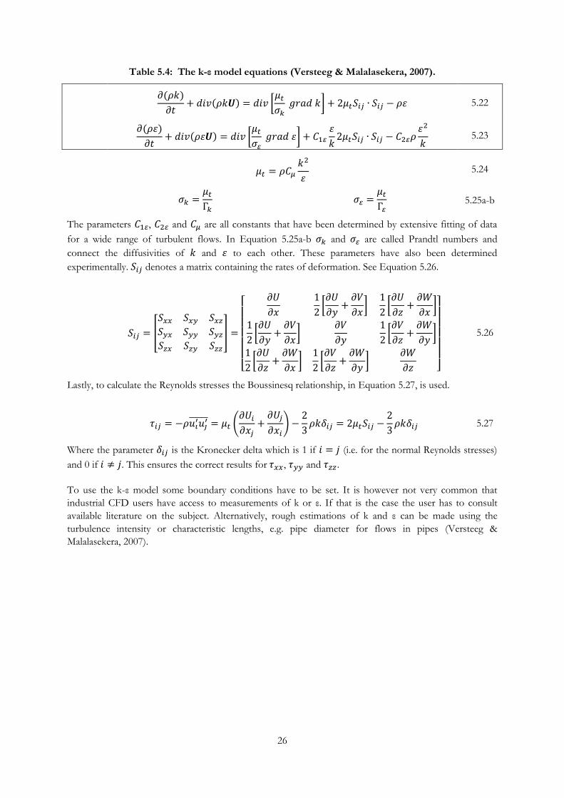
26

Table 5.4: The k-ε model equations (Versteeg & Malalasekera, 2007).

[

] 5.22

[

]

5.23

5.24

5.25a-b

The parameters , and are all constants that have been determined by extensive fitting of data

for a wide range of turbulent flows. In Equation 5.25a-b and are called Prandtl numbers and

connect the diffusivities of and to each other. These parameters have also been determined

experimentally. denotes a matrix containing the rates of deformation. See Equation 5.26.

[

]

[

[

]

[

]

[

]

[

]

[

]

[

]

]

5.26

Lastly, to calculate the Reynolds stresses the Boussinesq relationship, in Equation 5.27, is used.

(

)

5.27

Where the parameter is the Kronecker delta which is 1 if (i.e. for the normal Reynolds stresses)

and 0 if . This ensures the correct results for , and .

To use the k-ε model some boundary conditions have to be set. It is however not very common that

industrial CFD users have access to measurements of k or ε. If that is the case the user has to consult

available literature on the subject. Alternatively, rough estimations of k and ε can be made using the

turbulence intensity or characteristic lengths, e.g. pipe diameter for flows in pipes (Versteeg &

Malalasekera, 2007).

27

6 Commercial software for wind farm layout

optimization

In this work, three different programs were used to perform the simulations of the wind farms and the

power generation:

WAsP

WindPRO

WindSim

In this chapter the programs are scrutinized to provide some basic knowledge of the methods used, and it

can also serve as guidelines when working with the simulations.

6.1 WAsP

The WAsP software is developed for various wind applications ranging from wind analysis to siting of

wind turbines and calculating power production. It was introduced in 1987 by Risø National Laboratory in

Denmark and have since then become an industry standard for siting of wind turbines and wind resource

assessments. The energy calculation model in WAsP can be used in WindPRO to make calculations for

sites with complex terrain, which the available model ATLAS is insufficient for.

A flow model is used to calculate how the wind velocity is affected by the orographic features of the

terrain. The model used by WAsP is the BZ model by Troen in 1990 and is a further development of the

wind flow over hills work by Jackson and Hunt in 1975. It uses what is called a zooming polar grid,

meaning that the grid has its finest mesh at the center and is gradually decreased outwards. Further, the

resolution, or scale, of the grid is changing, or zooming, depending on the size of the domain. This size is

the distance from the center to the point furthest away on the map. A larger domain gives a larger size of

the grid. For example, the grid size near site center is about 2 m for a domain radius of 10 km and 10 m

for a 50 km radius. The length between each cell is increased by 6 % in the radial direction. Because of

these features it is important to have the most detailed and accurate description of the high contour lines

closest to the site center, preferably, according to WAsP, within “a km or so”. The requirement on the

detail level can be lowered further away from the center where the grid is coarser. The map should range

at least 5 km from any point where calculations are to be performed (Risø DTU, 2012).

The requirements on the roughness map is that it should extend at least 10 km from any point of interest,

and if any extensive water areas are present an extension should be made to at least 15 km.

WAsP uses a simplified model in the PARK module to calculate the wake effect from wind turbines in a

wind farm. Because of its simplicity it is computationally fast compared to other more advanced models.

The simplifications made in the model are performed by neglecting phenomenon’s occurring in the near

flow field of the rotor, the wakes are assumed to expand linearly with the distance away from the turbine

and the rule for overlapping wakes is simplified (Rathmann, et al., 2006).

6.2 WindPRO

WindPRO is a tool used in wind projects and it is developed by the Danish software and consultant

company EMD International A/S. The company has over 20 years of experience in wind turbine related

projects. The software is intended for wind project planning and design for projects ranging from a single

wind turbine up to large scale wind farms.

The program is module based meaning that there are modules with different purposes that can be

purchased depending on the specific demands of the user. The modules are categorized as follows:

28

Energy

Environmental

Visualization

Electrical

Economy

The especially interesting models for this work are in the energy category where the following modules are

available: METEO, MODEL, MCP, PARK, LOSS and OPTIMIZE.

6.2.1 METEO

The METEO module makes it possible to import and analyze wind data files. The data can be sorted in

and presented in different ways. It can for instance be used to identify errors in the measured data and

remove it. This data can then be used in the MODEL module.

6.2.2 MODEL

In MODEL the user can perform or import wind calculations to process in WindPRO and there are three

ways of doing this; by using ATLAS, WAsP or some external CFD software.

The ATLAS model is also developed by EMD international A/S and is already integrated into the

software. It is suitable for simple terrain and small scale projects when simple, fast and cost-effective

electricity generation calculations are required. It will not be used in this work as it is used for simple

terrain.

WAsP is a software developed by the Wind Energy Division at Risø DTU and can be used together with

WindPRO as an integrated part of the program. It is used to calculate wind speed distribution with the

wind atlas method. The required input data are wind statistics and terrain description (EMD International

A/S, 2012).

It is not possible to make CFD calculations directly with WindPRO but it is possible to interact with an

external CFD model by first preparing data in WindPro. The data can then be used by an external CFD

model to create a resource map that then can be imported back into WindPRO.

6.2.3 MCP

The MCP (measure correlate predict) module is used for long-term correction of measured data with four

common measure correlate predict methods. The methods are linear regression, matrix, weibull scale and

wind index. The module also includes downloadable wind data sets from the National Centers for

Environmental Prediction (NCEP) and the National Center for Atmospheric Research (NCAR) amongst

others.

6.2.4 PARK

The park module is used to calculate the electricity generation from multiple wind turbines. It is equipped

with three wake loss models (see chapter 2.1.7.1) used to compensate for the interaction between the wind

turbines. It is also possible to include different wind turbine models within the wind farm and test

different layouts against each other.

29

6.2.5 LOSS

The loss and uncertainty module is used to assess relevant losses according to recommendations of an

international group of experts. If the flow models used in previous calculations are known to be

insufficient as when used in complex terrain it is possible to try and correct for these errors by using

terrain ruggedness index (RIX) correction provided that RIX calculations was done in the PARK module.

6.2.6 OPTIMIZE

The optimize module is used to optimize the layout of the farm depending on what criterions are to be

met. These can for example be noise and specific layouts design options.

6.3 WindSim

The WindSim software was developed by the Norwegian company WindSim AS. It is a wind farm design

tool (WFDT) equipped with a three-dimensional graphical interface. WindSim employs a RANS solver in

three dimensions and is said to be appropriate for sites with a specific and complicated climatology as well

as for areas with complex and/or forested terrain (WindSim, 2011a).

The input data for the WindSim simulation is a terrain model of a size suitable for the particular project.

The model includes information about terrain orography, roughness and objects. In addition to this,

meteorological data from one or more points inside the modeled area has to be supplied (WindSim,

2011a).

The software is suitable for projects with different length scales ranging from micro siting of wind

turbines to meso scale wind resource assessments. Furthermore, WindSim utilizes body fitted coordinates

(adapted to follow the shape of the terrain or object) with increasing resolution closer to the ground.

When the above mentioned inputs are provided, WindSim can calculate the wind resources for the whole

site and the electricity generation from any number of wind turbines. A graphical layout of the site

including the wind turbines can be displayed directly in the visualization module (WindSim, 2011a).

6.3.1 Accuracy

The model requires the terrain map to be divided into a grid to be able to solve the numerical equations.

Hence, the accuracy of the results depends on the resolution of this grid. Unfortunately, the resolution is

limited by the available computational resources and cannot always reach the initially desired

specifications. For meso-scale modeling of vast landscapes a typical resolution can be 100x100 meters, and

10x10 meters could be appropriate for micro scale applications (WindSim, 2011a).

Since the numerical simulation takes place within a certain specified computational area, information

about the flow field at the border has to be supplied. The boundary conditions are set to fully developed

flow profiles adjusted with respect to the roughness of the terrain. However, this approach does not

capture any influences from the terrain outside the computational area. This could be abrupt changes in

topology (i.e. mountain ridges) and changes in roughness that alters the flow field. To account for this a

border zone can be created where the flow field is able to adjust to the surroundings (WindSim, 2011a).

To counter-act this problem it is also possible to use a nesting technique, where the results from an earlier

and larger model that totally encloses the specific area of interest is used as boundary conditions in a

smaller more refined model. The larger model can come from WindSim or from a mesoscale

meteorological model. (WindSim, 2011b).

30

6.3.2 Input data

The reliability of the numerical results is strongly dependent on the quality of the meteorological input

data. The longer the measuring period the more accurate the results, and in the case of short measuring

time periods a measure correlate predict (MCP) approach has to be taken. It is of great importance that

the measured data is representative for the whole computational domain, and in addition to this it has to

be suitable for the scale of the model. For example, it should not contain effects from large mountain

ridges or small local meteorological phenomena which are not captured by the numerical model. The

accuracy of the simulation can be greatly increased if more than one measurement position is available,

and there are several possible ways to utilize this in WindSim (WindSim, 2011a).

6.3.3 Using WindSim

The WindSim software is divided into several modules that enable the user to perform the necessary

measures in a step-wise manner (WindSim, 2011b). The modules are:

Terrain

Wind fields

Objects

Results

Wind resources

Energy

The following sub chapters include some information about how to use WindSim and the contents of the

above mentioned modules.

6.3.3.1 Terrain

The purpose of the terrain module is to create a three-dimensional area that encloses the site of the

planned wind farm. This area is defined by height variations and terrain roughness. Apart from this it is

also possible to model buildings and forested areas. The basis for the three-dimensional model is a two-

dimensional data sheet with roughness data and elevation, which has to be specified in advance (WindSim,

2011b).

The roughness length is by default obtained by WindSim from the two-dimensional data sheet, but a

constant value can also be set for the area to be modeled. For the numerical model in WindSim, as

mentioned above, the grid can be refined in areas of special interest. This means that the nodes will be

denser in that specific area and around its vicinity. The node density then decreases from its densest point

towards the borders, giving results with lower accuracy in these areas, but with a decreased need for

computational resources (WindSim, 2011b).

One important parameter that has to be set is the height above the terrain. It is defined as the distance

between the highest point on the terrain and the upper boundary of the computational domain. A suitable

value for this distance is a trade-off between two requirements, namely:

The node density in the vertical direction should be as high as possible for maximum accuracy (especially close to the ground), which suggests that the upper boundary should be placed as close to the ground as possible

If the upper boundary is placed too close to the ground it would block the flow over mountains as well as other high obstacles

31

When determining the height above the terrain WindSim suggests using a method that is based on the

open area (of air) above the entire terrain. The method states that the ratio between the minimum and

maximum open area (between the ground and the upper boundary) when traversing the model in the

west-east and south-north directions should exceed the value 0.95. See Equation 6.1.

6.1

The height above terrain can be set to meet this criterion automatically. A drawback with this approach is

however that for example a mountain ridge that crosses the computational domain diagonally might not

be detected as a significant variation in the open area since the procedure is to traverse in the east-west

and south-north direction. If this is the case it could lead to unnatural behavior of the fluid if the flow is

perpendicular to the ridge. The upper boundary of the computational domain then obstructs the flow as it

is too close to the ground leading to compression and acceleration of the fluid across the elevation

(WindSim, 2011b).

An important aspect to take into consideration is that the computational time required to reach a solution

is exponentially proportional to the number of cells in the grid. Here the nesting technique finds yet

another use, as splitting of the model into several smaller models can prove advantageous in terms of the

computational time needed. Apart from this, grid refinement could decrease computational times

considerably (WindSim, 2011b).

It is possible that the wind field simulation does not yield a physical solution, in other words; the solution

diverges instead of converging. The reason for this divergence can be the presence of rapid changes in

inclination between adjacent cells. Typically this occurs at narrow valleys or sharp mountain peaks. To

prevent divergence a technique called terrain smoothening can be applied. This automatic function smoothen

the terrain at all locations where the changes in inclination (i.e. the second order derivative of the height) is

higher than a certain predetermined value. This alters the terrain, but in most cases these locations are not

considered suitable for placing of wind turbines and hence a slight alteration can be tolerated. If used in

excess however, terrain smoothening changes the height of the terrain considerably and should because of

this be handled with care. Changes in height as well as in inclination is presented in the report generated

by WindSim and should be inspected to make sure that important areas has not been altered significantly

(WindSim, 2011b).

Another approach that may be used to achieve convergence with high inclination angles is to orthogonalize

the grid. By default the grid extends vertically along straight lines, but with grid orthogonalization the grid is

rearranged and extends vertically in curved lines with the aim of being perpendicular to the ground. This

result in that the cells become less tilted at locations with high inclinations. Orthogonalization is

recommended by WindSim when inclinations angles exceed 50°. It should however be pointed out that

the required simulation time will increase with orthogonalization activated (WindSim, 2011b).

When it comes to modeling forest in WindSim, there are two ways to include this in the simulations. One

option is to assign forested areas with a roughness length that is representative for the specific forest in

the grid file. The other alternative is to store all the forest characteristics under specific keywords in the

grid file and all data will then be read directly from it. One of the forest characteristics in the latter case is

the forest porosity, which is a value between 0 and 1. Where 0 would represent a completely open area and 1

corresponds to full flow blockage. The forest resistive force constants C1 and C2 may also be set, and are used to

model the forest as a resistive force either proportional to the velocity or proportional to the velocity

squared. See equations 6.2 and 6.3.

32

6.2

| | 6.3

Where S1 and S2 are the resistive forces (or source terms), is the air density and is the wind velocity.

is related to viscous forces and to pressure forces. Because of the high Reynolds numbers present in

these applications the pressure forces are much greater than the viscous (Crasto, 2006). Lastly, the forest cell

count in the vertical direction can be assigned a certain value. The cell distribution is uniform and the cell count

above the forest is simply the difference between the set value for the whole simulation and the cell count

for the forest.

6.3.3.2 Wind fields

The wind fields module is used to generate the wind database and simulates how the wind is affected by

the terrain. WindSim includes several numerical models to realize this, some featuring shorter computing

times as well as others focusing more on robustness. The wind fields in WindSim are generated by solving

the Reynolds Averaged Navier-Stokes equations using the k-ε turbulence model. The solved variables are

pressure, velocity, turbulent kinetic energy and turbulent dissipation rate. Additional variables may be

solved such as temperature, although this adds to the complexity of the model (WindSim, 2011b).

As mentioned earlier, the boundary and initial conditions in the form of a vertical velocity profile has to

be specified. This can be done either by setting it to correspond to an analytical wind profile based on the

log law, which depend on the roughness (and if temperature is included also the atmospheric stability), or

using the nesting technique. In many cases the log profiles are a bad assumption as boundary conditions,

as it assumes an infinite flat landscape outside the computational domain and nesting is strongly

recommend (WindSim, 2011b).

In the wind fields module the height of the boundary layer has to be set. Above this level is the geostrophic

domain where the wind profile is constant. Another parameter is the boundary condition at top. This could be

set to meet a fixed pressure condition or to a frictionless wall. For simulations in complex terrain the fixed

pressure condition should be used, whereas the frictionless wall is more suitable for flat terrain (WindSim,

2011b).

The temperature equations can be activated in the wind fields module, and depending on what type of

initialization is chosen different boundary and initial conditions are set. The temperature equations can be

initialized by giving a value for the Monin-Obukhov length or by assuming a log profile at the inlets. In

the first case a linear temperature gradient is assumed in the atmosphere and in the second case the

temperature gradient is assumed constant throughout the atmosphere (WindSim, 2011b).

The standard k-ε model is the default turbulence model used in WindSim, but there are other

modifications available as well. Apart from this, the Coriolis force can also be included in the simulations

(WindSim, 2011b).

Regarding the numeric solver in WindSim, there are two available options. The first one being the

segregated solver, which is based on the Patankar-Spalding SIMPLE (Semi-Implicit Method for Pressure

Linked Equations) algorithm. This involves solving the velocity and pressure parts of the flow equations

separately. The other alternative is the coupled solver. It is a multi-grid solver which simultaneously solves

the hydrodynamic variables in a whole-field manner (WindSim, 2011b).

33

With the segregated solver it is possible to solve a larger model on a certain machine compared to the

coupled solver. This can however require as much as ten times the iterations as for the coupled solver, and

thus the segregated solver should be used when longer computational times can be accepted. The

iterations are actually quicker using the segregated solver, but the solution generally takes longer to

converge (WindSim, 2012c). For example models with 1000000 cells might need more than 1000

iterations to converge whereas the coupled solver can converge after less than 100 (WindSim, 2011b).

In cases where convergence is hard to achieve WindSim has an inbuilt convergence wizard that can be

used to resolve these issues. The default false time-step relaxation is then substituted with an automatic

linear-under-relaxation technique (WindSim, 2011b).

6.3.3.3 Objects

In the objects module different objects are placed within the model. The position of the turbines,

climatologies and transferred climatologies is set, and it is possible to view geometrical objects in the

three-dimensional model as well. These objects can be set to be visible or invisible, which determines

whether the object is taken into account in the energy and wind resource calculations or not (WindSim,

2011b). A transferred climatology is a virtual set of measurements generated from a real climatology and

the numerical database from the simulation. This enables the user to simulate and map different wind

conditions from one point to another (WindSim, 2012d). It should be noted that a transferred climatology

(within the same model) does not provide any new information and hence is not used neither in the

calculations preformed in the wind fields module nor the energy module (described below). A transferred

climatology from an external model does however provide new information, and may be imported to

utilize in the present one. Moreover, specifications such as the power curve, hub height, rotor diameter,

rotational speed and the direction towards which the wind turbines are turned can be set in the object

module (WindSim, 2011b).

6.3.3.4 Results

Flow variables such as wind speed, direction, turbulence intensity and the vertical component of the wind

can all be viewed in the results module. The results can be displayed for a specific point in the model by

choosing the sector and the height above ground.. The result module extracts two-dimensional horizontal

planes from a reduced database that was generated during the wind fields simulations. The term “reduced”

meaning that this database only contains data up to a certain height previously specified by the user in the

wind fields module (WindSim, 2011b).

The flow variable can also be shown as normalized values. Normalization means that the flow variable is

divided by a certain value, and the available normalization variables are amongst others: scalar speeds in

the x, y and z direction; velocity vectors in two and three dimensions; scalar wind directions; turbulent

kinetic energy, intensity and dissipation rate; relative pressure and lastly the wind shear exponent. It is

possible to normalize the results against either a scalar value or against the nearest climatology (WindSim,

2011b).

6.3.3.5 Wind resources

In the wind resources module the generated wind data base is weighted against measurements and a wind

resource map is produced. The wind resource map is then later used in the energy calculations. One or

several measurements can be used to produce the wind resource map, and when more than one

measurement is available the map will be established via interpolation. Besides this, the wind resource

module includes an area classification feature. It can identify interesting areas in the model, with regards to

size and wind speeds. Additionally, the possible power production in these areas can be estimated

(WindSim, 2011b).

34

When it comes to wake effects and the different models available in WindSim, there are three choices. The

Jensen model, the Larsen model and the model proposed by Ishihara, Yamaguchi and Fujino (Ishihara, et

al., 2004). All of the above are analytical models which is especially attractive in terms of reduced

computational times compared to CFD based models. The wake models use the results generated in the

wind fields module in WindSim to calculated the velocity deficit after the turbines. Thus, the wake-wake

and wake-terrain interactions are not described correctly seeing as these effects are not taken into account

in the wind fields module. One way to incorporate said aspects are to create models for each turbine in the

terrain module, which then would be part of the wind field simulations (WindSim, 2011b).

6.3.3.6 Energy

The energy module is used to calculate the annual electricity generation and the wake losses associated

with each turbine. It is also possible to compare different park layouts in this module. More than one

climatology can be used to determine the expected electricity generation, this is however done separately

for each one. The results with the different climatologies as input can then be compared easily. The

climatologies is given both in the form of a frequency distribution and its Weibull distribution, and the

electricity production is calculated for both these cases (WindSim, 2011b).

The air density at the positions of the turbines is a parameter that can be set in the energy module, and as

the wind turbine power curve is provided for a predetermined density a correction term is applied if these

densities differ from each other. There are two methods for correcting the power curve for an alternative

density according to the IEC standard EN 61400-12. For pitch-regulated turbines the original power

curve is used and the wind speed is corrected. The correction is made by multiplying the wind speed with

the fraction between the air density specified in the energy module, and the one in the power curve, at one

third of the rated power. For stall-regulated turbines the density fraction is simply multiplied with the

reference power curves. After the calculations have been made the vertical wind profiles can be exported

in an ASCII file and viewed for every wind turbine position. In addition to this the rotor profiles are also

available for export (WindSim, 2011b).

35

7 Methodology

As previously stated, two commercial wind energy calculation software are to be evaluated and compared

to investigate their reliability in a forested wind park in Sweden. The software evaluated in this report is

WindPRO and WindSim, where WindPRO is used together with the software WAsP to perform the wind

flow calculations.

There are a number of steps involved in the wind energy calculations and these steps will be explained in

this section. It is of great importance to perform these steps with caution to reduce the uncertainties and

ensure as reliable results as possible within the time limit of the project.

Firstly the wind data must be analyzed and processed before it can be used in both WindPRO and

WindSim. Secondly the site is to be analyzed with respect to its terrain and topography. All information

about the site is then to be processed in WindPRO. This map description is then exported and used as

input in WindSim where further improvements and adjustments are required for the energy calculations.

An overview of the available data is illustrated in Figure 7.1. Operation refers to when production data is

available from the wind turbines. SODAR denotes when there is available data from wind measurements.

It is Site A that was simulated in this study. Site B is only used to adjust the data and results between the

time periods.

Figure 7.1: Timeline of the available data.

7.1 Using the simulation tools

A description of the site’s terrain was created in WindPRO to enable the wind simulations to account for

terrain properties. The terrain description was used by both WindPRO/WAsP and WindSim for the

energy calculations. The level of detail varies in these terrain descriptions depending of the requirements

of the user and the available details of the maps. The scale and size of the background maps used as input

for Site A in WindPRO are:

1:250 000 - 40 km x 40 km

1:100 000 - 27.7 km x 28.2 km

1:50 000 - 15.1 km x 13.8 km

1:12 500 - 4 km x 4.8 km

7.1.1 Terrain properties

There are three different types of terrain specific information that is accounted for in the wind model.

This is the orography, the roughness of the terrain and obstacles. The orography and roughness is

described with contour lines on the map where each line gives information about the terrain. No obstacles

were used in this work.

36

7.1.1.1 Orography

The contour lines are manually entered using the Line Object in WindPRO with the background maps

used as reference. The height contour lines for the two highest scale maps have a resolution of 5 meters.

The terrain surface height in-between the height contour lines are calculated by WindPRO using a method

called triangulated irregular network (TIN). There are three available options and different two methods for

calculating TIN. The chosen option is the one set as default by WindPRO and is called “TIN on the fly”.

It calculates during the progress of the work and is using a method where TIN is calculated for the whole

file instead of a predetermined radius, which is the case in the other method. Further, the other method

has problems with triangles crossing contour lines and cannot handle single point contours.

The height contour map created in WindPRO had a final size of 15.1 x 13.8 km. The file was converted

into the WAsP format .map to enable the file to be imported into WindSim.

A map of the final orography can be seen in Figure 7.2. Site A is located inside the black circle. The

highest point on the map is 500 m and the lowest is 145 m.

Figure 7.2: An orographic map of the terrain created in WindPRO with a resolution of 18 m.

In Figure 7.2 the height above the sea level in meters is displayed to the left in a color spectrum ranging

from purple to red. The location of the wind farm is marked with a black circle.

37

A more detailed orographic map of Site A, inside the black circle above, is depicted in Figure 7.3.

Figure 7.3: Detailed orographic map of the terrain in Site A created in WindPRO with a resolution of 6 m.

7.1.1.2 Roughness and WindSim forest module

The roughness map is created manually by using the Area Object in WindPRO to draw polygons and

define a roughness length of the area inside the polygon. A background roughness is set, and this is the

roughness length for all areas that is not defined by the user. The finished polygons are converted to

roughness lines and used in the Line Object.

The roughness length for a specific area was determined by observing the vegetation and classifying it

through satellite images from Google Maps. The satellite images are dated to year 2009. To speed up the

drawing process and possibly increase the accuracy, satellite images was merged from Google Maps and

imported as a background map using the MAPDEF function and setting coordinates according to the

previously entered maps. The size of the final roughness map is 15.5 km x 15.5 km.

In WindSim the forest roughness can be chosen to not be represented by only a roughness length. Instead

the forest module is used where other parameters are also configured for the forest. The forested areas are

created by choosing a roughness length that shall be interpreted as forest. When importing the created

roughness map all areas with these specified roughness lengths is then converted into forest blocks. To

ensure that non-forested areas with the same roughness length as forest is not interpreted as forest, the

roughness length is changed to a value close to the same value. For example, if village and forest have the

same roughness length, 0.4 m, the roughness length of the village is set to 0.399 m instead of 0.4 m.

38

7.1.1.3 Turbines and Wind Measurement

The wind farm consists of five wind turbines and they were defined in WindPRO using Insert New WTG

and as a new Object in WindSim according to the coordinates provided by DalaVind AB. The wind

turbine manufacturer is Vestas and the model is called V90-2.0 MW. It is specified to a hub height of 105

m with a rotor diameter of 90 m. The rated power is 2 MW and the noise classification is 0. The power

curve is dated to 2005-06-27 and was provided by Vestas through WindPRO.

The name and numbering of the wind turbines (VKV is short for vindkraftverk, which means wind

turbine in Swedish) are as follows:

VKV1 – Ellen

VKV2 – Henrika

VKV3 – Alma

VKV4 – Östen

VKV5 – Gisela

As previously stated, two measurements have been performed on Site A using SODAR equipment. The

measurement series are from two different time periods, one from 2008/2009 and the other from 2011.

Exact placement of the SODAR measurements and the wind turbines can be seen in Figure 7.4. The red

three legged figures are the wind turbines and the orange/grey three legged figures is the wind

measurements. Note that the first and the second measurments was not performed on the same location.

The second measurement was performed at a distance of about 435 m north east of the first location.

39

Figure 7.4: The layout of the wind turbines and the placement of the wind measurements.

The 2008/2009 measurement was performed from 2008-10-22 to 2009-10-29, a total of 372 days. No

wind turbines had been installed during this period. The turbines were erected in 2010 and were put into

operation in August/September the same year. The 2011 data is from the period 2011-05-01 to 2011-07-

31. This means that the wind turbines were operating at the time of the measurements which indicates

that the data is influenced by the wakes induced by the wind turbines.

7.1.2 General parameters

The air density was set to 1.200 kg/m3 and was determined in WindPRO by choosing “Adjust to

individual WTGs based on elevation and hub height” and then choosing “Climate data from climate

station database” and selecting the closest climate station, located 59 km away.

The power curve correction method in WindPRO was set to be “New WindPRO method (adjusted IEC

method, improved to match turbine control)” and this method is also recommended by WindPRO. It is a

further development of the IEC 61400-12 method of correcting power curves.

WindSim have only one option for correcting power curves and is to use the IEC 61400-12 correction

method. This should however not influence the results as both methods of correcting can be used when

there are only small density changes are present. The reference density specified for the power curve is

1.225 kg/m3 and the difference from the average density used in the calculations is only 2 %.

40

7.1.3 WindSim settings and convergence

Two different numbers of cells were used when testing the numerical model. The first simulation was

done with 1,000,000 cells and the second simulation was done with 2,500,000 cells. The energy results

only differed with 0.2 % between the two meshes. Convergence plots for the two initial test runs can be

seen in appendix A. After this initial test it was decided that the finer grid with 2.5 million cells was to be

used for the simulations simply because the required computational resources were available. The finest

resolution was 16.5 x 16.6 m, and the model had had 20 cells in the z-direction extending 3010.5 m above

the point in the model with the highest elevation. The grid can be seen in Figure 7.5 and was chosen to be

refined, thus not a homogeneous grid. The refinement area was centered on Site A (slightly northeast

from the map center). To determine the height above the terrain, the built-in automatic function was used,

and orthogonalization as well as smoothing of the grid was not enabled. The remaining values in the

terrain module were set to default with the exception of the forest settings that were varied when testing

different cases. In Figure 7.5 the grid is viewed from southeast in 3D (left) and directly from above (right).

Figure 7.5: The refined grid generated in WindSim.

In the Wind Fields module the model was split into 12 uniformly distributed sectors, and the height of the

boundary layer was kept at the default value of 500 m. Similarly, the speed above the boundary layer was

set to 10 m/s (default value). The boundary condition at the top of the model was set to “fixed pressure”

and no nesting was performed. When it comes to the physical models used the potential temperature (see

chapter 4.1) was disregarded, the air density was set to 1.2 kg/m3 and the standard k- model was selected

for turbulence closure. The coupled solver was used in all of the simulations and most of the time two

sectors were solved simultaneously.

For the different simulation cases, the number of iterations needed for convergence of the spot values

varied between 80 and 150, see Figure 7.6. Generally, more iterations were needed for the residual values

to reach an acceptable level than what was required for the spot values to converge. The residual values

reached a satisfactory level after around 160 to 180 iterations, see Figure 7.7. Initially all sectors were run

for 120 iterations after which the spot values and the residual values were inspected to determine which

sectors needed more iterations. The field value animation feature was also used to make sure that all areas

of the computational domain had converged. This process was repeated for all the simulations carried out

in WindSim. In Figure 7.6 and Figure 7.7, the variables are scaled according to the minimum and

maximum values that can be seen on the right. , , and are the velocities in the x-, y- and z-

direction respectively, denotes the turbulent kinetic energy and lastly, refers to the turbulent

dissipation rate.

41

Figure 7.6: Convergence of the spot values in WindSim. Convergence was achieved after around 80 iterations (top) to 150 iterations (bottom).

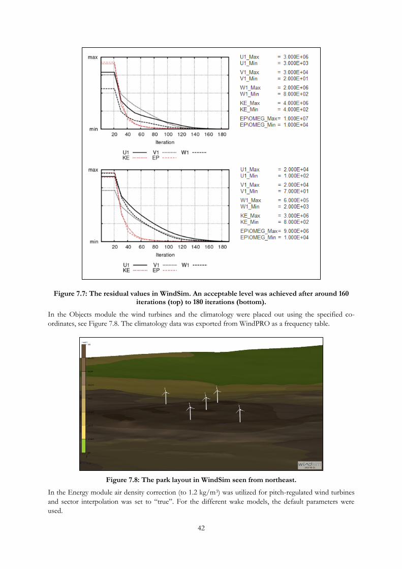
42

Figure 7.7: The residual values in WindSim. An acceptable level was achieved after around 160 iterations (top) to 180 iterations (bottom).

In the Objects module the wind turbines and the climatology were placed out using the specified co-

ordinates, see Figure 7.8. The climatology data was exported from WindPRO as a frequency table.

Figure 7.8: The park layout in WindSim seen from northeast.

In the Energy module air density correction (to 1.2 kg/m3) was utilized for pitch-regulated wind turbines

and sector interpolation was set to “true”. For the different wake models, the default parameters were

used.

43

7.2 Treating the measured data

The wind data was analyzed and processed from the SODAR measurements. The data was provided as a

text file with information about wind speed, wind direction, standard deviation of the wind speed, vertical

velocity, standard deviation of the vertical velocity and the quality of the signal (signal-to-noise ratio). This

information was available from 20 meter to 150 meter above ground level with a resolution of 5 meters.

Two measurement periods where available, one with the duration of 1 year and the other for 3 months,

with data provided with a time step of 10 minutes.

To ensure good quality of the data the manufacturer has specified an upper limit on the signal-to-noise

ratio for what is an acceptable and reliable measurement. Data that does not fulfill this requirement is

given an error code (9999) that is displayed instead of the unreliable value. The error codes and other

obvious false readings are excluded from any energy calculations.

Availability of the data in the two measurement series are presented in Table 7.1. All measured heights are

represented in the table and the availability is shown for the horizontal wind speed and its standard

deviation.

44

Table 7.1: Availability of the wind measurements from the SODAR device.

2008/2009 2011

Height Wind speed Standard deviation

Wind speed Standard deviation

20 99.26% 83.85% 99.58% 60.33%

25 99.32% 86.65% 99.60% 64.77%

30 99.30% 88.76% 99.57% 67.86%

35 99.23% 89.36% 99.52% 70.13%

40 99.21% 90.24% 99.48% 72.16%

45 99.29% 91.16% 99.44% 73.74%

50 99.47% 97.27% 99.61% 0.00%

55 99.16% 94.13% 99.57% 76.97%

60 98.86% 93.64% 99.52% 71.85%

65 98.64% 92.98% 99.43% 68.09%

70 98.51% 92.57% 99.35% 64.80%

75 98.47% 92.33% 99.44% 61.46%

80 98.53% 91.83% 99.40% 59.06%

85 98.58% 91.52% 99.32% 56.67%

90 98.59% 91.10% 99.15% 53.17%

95 98.56% 90.61% 99.09% 50.75%

100 98.48% 90.04% 99.01% 48.04%

105 98.08% 89.45% 98.85% 45.32%

110 97.71% 88.86% 98.52% 41.97%

115 97.21% 88.17% 98.04% 39.90%

120 96.64% 87.41% 97.39% 37.61%

125 95.93% 86.45% 96.06% 35.48%

130 95.18% 85.46% 94.29% 32.20%

135 94.36% 84.37% 92.31% 30.22%

140 93.41% 82.99% 89.89% 27.77%

145 92.43% 81.80% 87.50% 25.28%

150 91.46% 80.47% 84.44% 23.40%

Total 97.55% 89.02% 97.31% 50.33%

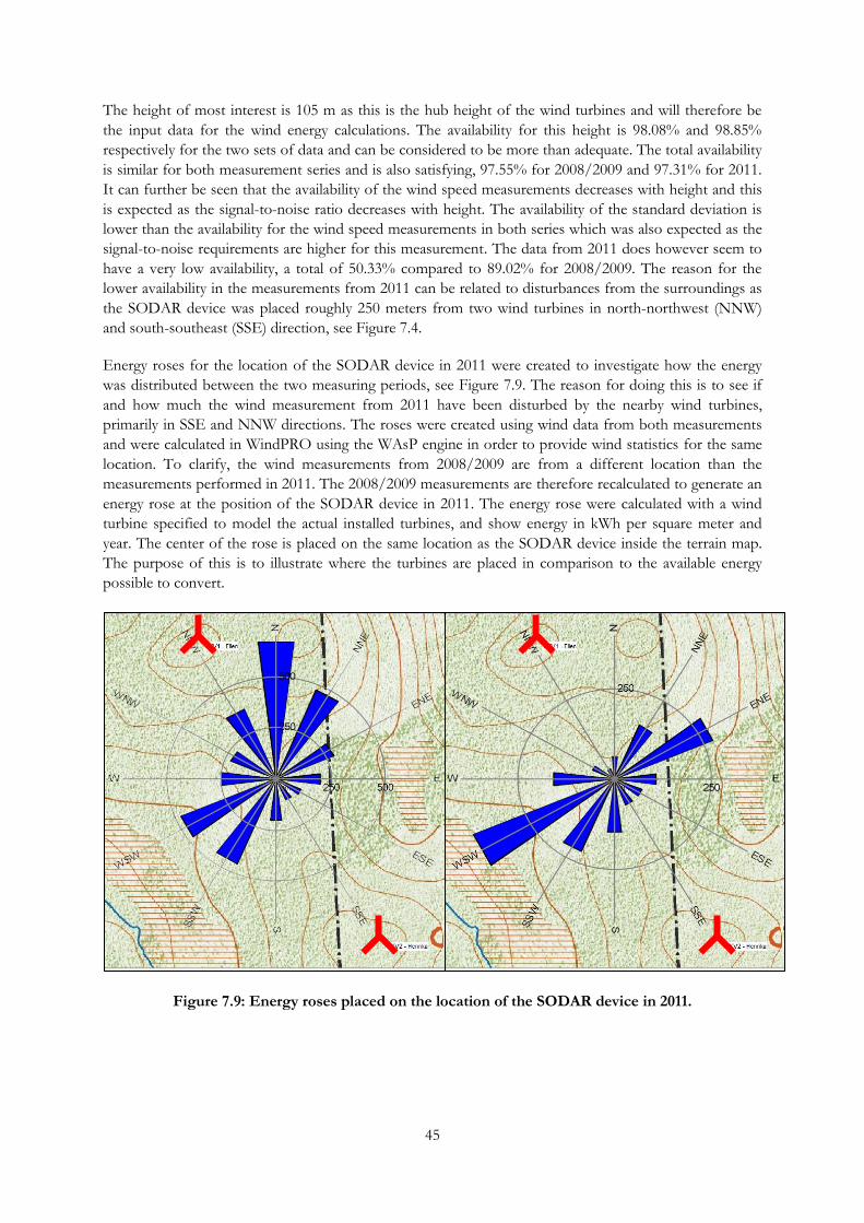
45

The height of most interest is 105 m as this is the hub height of the wind turbines and will therefore be

the input data for the wind energy calculations. The availability for this height is 98.08% and 98.85%

respectively for the two sets of data and can be considered to be more than adequate. The total availability

is similar for both measurement series and is also satisfying, 97.55% for 2008/2009 and 97.31% for 2011.

It can further be seen that the availability of the wind speed measurements decreases with height and this

is expected as the signal-to-noise ratio decreases with height. The availability of the standard deviation is

lower than the availability for the wind speed measurements in both series which was also expected as the

signal-to-noise requirements are higher for this measurement. The data from 2011 does however seem to

have a very low availability, a total of 50.33% compared to 89.02% for 2008/2009. The reason for the

lower availability in the measurements from 2011 can be related to disturbances from the surroundings as

the SODAR device was placed roughly 250 meters from two wind turbines in north-northwest (NNW)

and south-southeast (SSE) direction, see Figure 7.4.

Energy roses for the location of the SODAR device in 2011 were created to investigate how the energy

was distributed between the two measuring periods, see Figure 7.9. The reason for doing this is to see if

and how much the wind measurement from 2011 have been disturbed by the nearby wind turbines,

primarily in SSE and NNW directions. The roses were created using wind data from both measurements

and were calculated in WindPRO using the WAsP engine in order to provide wind statistics for the same

location. To clarify, the wind measurements from 2008/2009 are from a different location than the

measurements performed in 2011. The 2008/2009 measurements are therefore recalculated to generate an

energy rose at the position of the SODAR device in 2011. The energy rose were calculated with a wind

turbine specified to model the actual installed turbines, and show energy in kWh per square meter and

year. The center of the rose is placed on the same location as the SODAR device inside the terrain map.

The purpose of this is to illustrate where the turbines are placed in comparison to the available energy

possible to convert.

Figure 7.9: Energy roses placed on the location of the SODAR device in 2011.

46

In Figure 7.9 the energy rose to the left is calculated using wind data from 2008/2009 (undisturbed), and

the right energy rose is calculated with data from 2011 (disturbed). Red three legged figure represents a

wind turbine. The bars show energy in kWh per m2 and year. It can be seen in both roses that the energy

distribution in the wind coming from SSE is similar. The wind energy from WNW, NNW and N is

however greatly reduced in 2011 compared to 2008/2009. The most pronounced change is wind energy

from the North. This wind direction accounts for the most energy in 2008/2009 and is the second

smallest in 2011.

The wind speed was also analyzed to see how it differs between the years. A table of the mean wind speed

for all directions from both measurements is presented in Table 7.2. It is calculated with the WAsP engine

as previously stated. The difference for 2011 and 2008/2009 is shown in comparison with the mean wind

speed, as well as the total difference in percentage points.

Table 7.2: Comparison of the mean wind speed [m/s] for all wind directions between 2008/2009 and 2011.

Bold text denotes the three wind directions with largest differences, and rows for the wind directions of

most interest are marked with gray.

2011

Difference to mean

wind speed

2008/2009

Difference to mean

wind speed

Difference between years in

percentage points

N 5.12 -10.49% 9.87 31.60% -42.09

NNE 6.02 5.24% 8.86 18.13% -12.89

ENE 6.25 9.27% 8.04 7.20% 2.07

E 5.2 -9.09% 7.22 -3.73% -5.36

ESE 5.18 -9.44% 6.59 -12.13% 2.69

SSE 5.4 -5.59% 6.35 -15.33% 9.74

S 6.24 9.09% 6.71 -10.53% 19.62

SSW 5.62 -1.75% 6.93 -7.60% 5.85

WSW 6.17 7.87% 7.16 -4.53% 12.40

W 5.74 0.35% 6.57 -12.40% 12.75

WNW 4.99 -12.76% 6.97 -7.07% -5.70

NNW 4.47 -21.85% 8.42 12.27% -34.12

Mean 5.72

7.5

The table shows that the largest differences are in the N, NNW and S directions. In N and NNW there is

a reduction in the wind speed for 2011 and in the S direction there is an increase. In SSE where the wind

turbine is placed the wind speed have increased.

47

7.2.1 Actual electricity production and correction

Information about the actual amount of electricity generated by the wind turbines in 2011 have been

provided by DalaVind AB. The production data is listed in an Excel document and contains the electricity

production for all the wind turbines in separate columns. The recorded period ranges from 2011-01-01 to

2011-12-31 with a time step of 10 minutes. The availability of the production data is 99.93%. The

calculation of the availability is only accounting for when the production data shows zero in generated

electricity. This means that “availability” here may include periods when the turbine actually is available

but generates zero electricity. Negative values in the production data are present for certain time periods

with low wind speeds when the turbines are using electricity from the grid. These negative values are

removed from the dataset as the calculations in WindPRO and WindSim is set not to account for negative

energy flows, it could however be done by specifying it in the power curve below the cut in speed.

The mean wind speed is changing from year to year and a direct comparison between the real production

data and the simulated production can be misleading and can therefore be corrected to give a better

representation of the data. The method used in this study is to account for the differences by introducing

a correction factor. This factor can be obtained from Vindstat which is an ongoing project by the Swedish

Energy Agency. Operating information from wind turbines in Sweden is collected, compiled and then

presented in monthly and yearly reports. The statistics is currently (spring 2012) covering 67% of all the

wind turbine generated electricity.

Included in this report is what is called the “vindindex”, which translates to “wind index”, and shows the

energy content of the wind during each year from 1991 to 2011. It is presented as a percentage of the

average year. The SODAR measurement used in the study is from both 2008 and 2009 where roughly two

months are from 2008. As there is only two months from 2008 the indexed is used for 2009 and will

represent this period.

A preliminary report for 2011 was available from Vindstat AB and the chart for the wind index is shown

in Figure 7.10.

Figure 7.10: Energy content in the wind for Sweden during 1991-2011 (Carlstedt, 2012).

The correction factor calculated using this chart would for year 2011 and 2009 become 0.81. This index is

calculated from wind turbines scattered all over Sweden and thus the data may not be a good

representation of the wind conditions at Site A. More detailed information of the operation is available in

the report and is broken down for separate counties. It shows the number of turbines, power, generated

electrical energy and wind index from 2006 to 2011. The information for Dalarna is presented in Table

7.3.

48

Table 7.3: Detailed operation information for Dalarna county from 2006 to 2011 (Carlstedt, 2012).

2006 2007 2008 2009 2010 2011

Wind turbines 3 3 7 7 14 34

Power (MW) 2.6 2.6 8.45 29.45 41.3 64.3

Energy (MWh) 5673 9539 17203 64445 82643 124269

Wind index (%) - - - - 92 80

The data for 2006 to 2009 is only available with three and seven wind turbines and the Swedish wind

index is not included for these years. Year 2010 and 2011 is however available with more turbines and can

be compared with the Swedish wind index. For 2011 the Swedish index is 116% and it is 80% for Dalarna.

For 2010 the Swedish index is 90% and 92% for Dalarna. It can be noted that the wind farm on Site A, as

well as another wind farm located on Site B, not far away from Site A and also in connection with

DalaVind AB, is included in these statistics. This comparison indicates that the wind index for Sweden

cannot be used to correct the wind data from 2008/2009 and the production year of 2011 for Site A.

Another way of attaining a correction factor is to simply use the data from a wind farm located in the

vicinity of the site by comparing the electricity generation from 2008/2009 with 2011. A site suitable for

this comparison is the previously mentioned wind farm on Site B. DalaVind among others are currently

operating this wind farm located roughly 30 km away from Site A. It was in operation during the wind

measuring period and the production year of 2011. The wind farm consists of five Vestas V90 turbines

with a hub height of 95 m (the turbines on Site A has a hub height of 105 m). The terrain for both sites is

depicted in Figure 7.11 and Figure 7.12. It can be seen that the sites are similar in terms of complexity of

the terrain. Furthermore, both sites are located at about 400 m above sea level. The turbines are not

depicted in these figures but all of them are located on high ground.

Figure 7.11: A map of the terrain for Site A, the circle marks the site (Hitta.se, 2012).

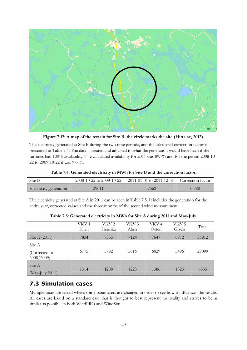
49

Figure 7.12: A map of the terrain for Site B, the circle marks the site (Hitta.se, 2012).

The electricity generated at Site B during the two time periods, and the calculated correction factor is

presented in Table 7.4. The data is treated and adjusted to what the generation would have been if the

turbines had 100% availability. The calculated availability for 2011 was 89.7% and for the period 2008-10-

22 to 2009-10-22 it was 97.6%.

Table 7.4: Generated electricity in MWh for Site B and the correction factor.

Site B 2008-10-22 to 2009-10-22 2011-01-01 to 2011-12-31 Correction factor

Electricity generation 29611 37562 0.788

The electricity generated at Site A in 2011 can be seen in Table 7.5. It includes the generation for the

entire year, corrected values and the three months of the second wind measurement.

Table 7.5: Generated electricity in MWh for Site A during 2011 and May-July.

VKV 1 Ellen

VKV 2 Henrika

VKV 3 Alma

VKV 4 Östen

VKV 5 Gisela

Total

Site A (2011) 7834 7335 7124 7647 6972 36912

Site A

(Corrected to 2008/2009)

6175 5782 5616 6029 5496 29099

Site A

(May-July 2011) 1314 1288 1223 1386 1325 6535

7.3 Simulation cases

Multiple cases are tested where some parameters are changed in order to see how it influences the results.

All cases are based on a standard case that is thought to best represent the reality and strives to be as

similar as possible in both WindPRO and WindSim.

50

7.3.1 Simulation cases 2008/2009

The simulation cases based on the measurements performed at Site A during the period 2008-10-22 to

2009-10-22 are presented in this section. In Figure 7.13 it can be seen that no production data was

available during the SODAR measurements at Site A in 2008/2009. This is because as mentioned above,

the actual wind turbines were not installed until August/September 2010. Operation data from Site B is

available during the entire period, 2008-2012. The simulation results from the 2008/2009 cases are thus to

be verified using operational data from Site A and Site B. This is achieved by comparing the production of

Site B in 2011 and 2008/2009 to obtain a correction factor (see Figure 7.13 and Chapter 7.2.1). This

correction factor is then used to translate the operation data from Site A in 2011 into a theoretical value of

the production for Site A during time period of the SODAR measurement (left side of Figure 7.13)

Figure 7.13: Timeline for simulation cases 2008/2009.

Even though the two sites are similar in terms of orographic and roughness related characteristics (hilly

landscape, tree species), not to mention that both parks have five turbines rated 2 MW, they still remain

two quite different sites influenced by their own topography and surrounding environment. Because of

this the 2008/2009 simulation results should not be compared to the operation data of Site B directly, but

instead the approach is to use operation data from Site A in 2011 and adjust it to the time period of the

SODAR measurements 2008/2009, as described above.

7.3.1.1 Standard cases

The standard cases will to a large extent use the same parameters in both WindSim and WindPRO with

the aim of determining the differences in the results generated by the two programs. In this work, there

are three standard cases:

1. WindPRO standard case

2. WindSim standard case RH

3. WindSim standard case FM

Here, RH is short for roughness height and FM abbreviates forest module. The roughness lengths used to

define the terrain in WindPRO standard case and WindSim standard case RH is described in Table 7.6.

RESULTS

VERIFICATION

CORRECTION

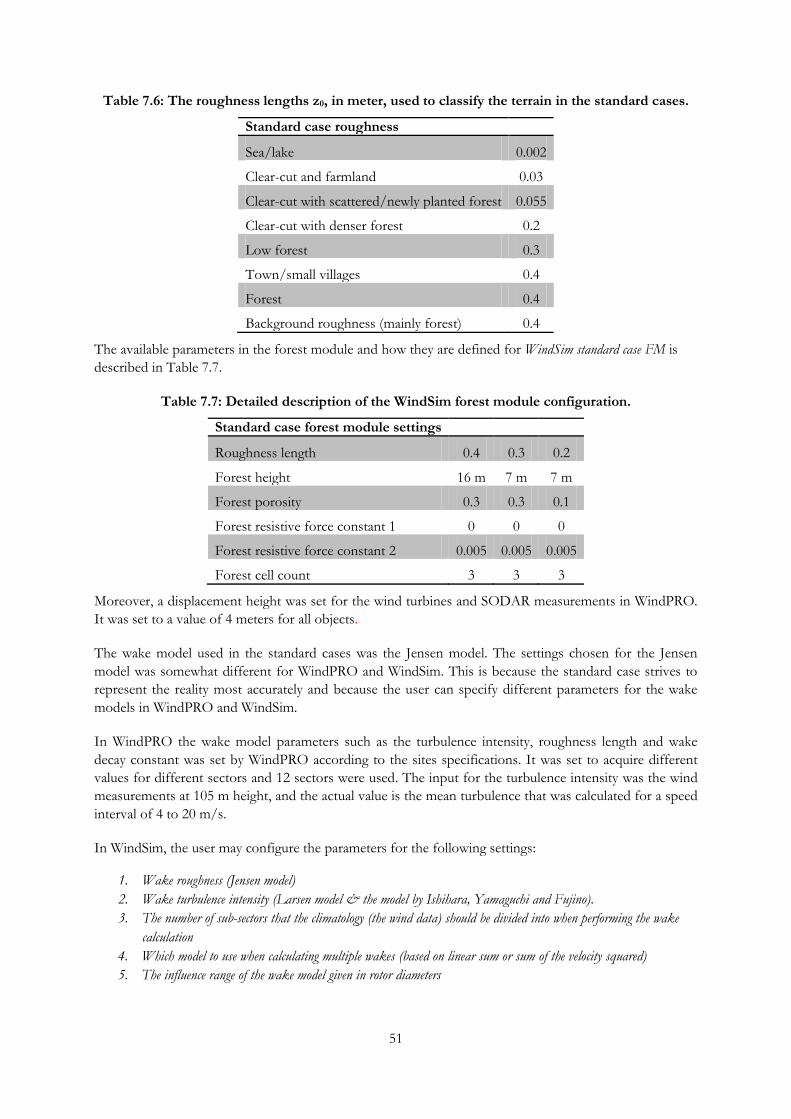
51

Table 7.6: The roughness lengths z0, in meter, used to classify the terrain in the standard cases.

Standard case roughness

Sea/lake 0.002

Clear-cut and farmland 0.03

Clear-cut with scattered/newly planted forest 0.055

Clear-cut with denser forest 0.2

Low forest 0.3

Town/small villages 0.4

Forest 0.4

Background roughness (mainly forest) 0.4

The available parameters in the forest module and how they are defined for WindSim standard case FM is

described in Table 7.7.

Table 7.7: Detailed description of the WindSim forest module configuration.

Standard case forest module settings

Roughness length 0.4 0.3 0.2

Forest height 16 m 7 m 7 m

Forest porosity 0.3 0.3 0.1

Forest resistive force constant 1 0 0 0

Forest resistive force constant 2 0.005 0.005 0.005

Forest cell count 3 3 3

Moreover, a displacement height was set for the wind turbines and SODAR measurements in WindPRO.

It was set to a value of 4 meters for all objects.

The wake model used in the standard cases was the Jensen model. The settings chosen for the Jensen

model was somewhat different for WindPRO and WindSim. This is because the standard case strives to

represent the reality most accurately and because the user can specify different parameters for the wake

models in WindPRO and WindSim.

In WindPRO the wake model parameters such as the turbulence intensity, roughness length and wake

decay constant was set by WindPRO according to the sites specifications. It was set to acquire different

values for different sectors and 12 sectors were used. The input for the turbulence intensity was the wind

measurements at 105 m height, and the actual value is the mean turbulence that was calculated for a speed

interval of 4 to 20 m/s.

In WindSim, the user may configure the parameters for the following settings:

1. Wake roughness (Jensen model)

2. Wake turbulence intensity (Larsen model & the model by Ishihara, Yamaguchi and Fujino).

3. The number of sub-sectors that the climatology (the wind data) should be divided into when performing the wake

calculation

4. Which model to use when calculating multiple wakes (based on linear sum or sum of the velocity squared)

5. The influence range of the wake model given in rotor diameters

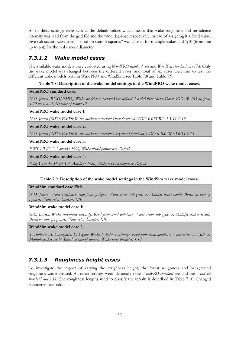
52

All of these settings were kept at the default values which meant that wake roughness and turbulence

intensity was read from the grid file and the wind database respectively instead of assigning it a fixed value.

Five sub sectors were used, “based on sum of squares” was chosen for multiple wakes and 1;10 (from one

up to ten) for the wake rotor diameter.

7.3.1.2 Wake model cases

The available wake models were evaluated using WindPRO standard case and WindSim standard case FM. Only the wake model was changed between the different cases, and total of six cases were run to test the different wake models both in WindPRO and WindSim, see Table 7.8 and Table 7.9.

Table 7.8: Description of the wake model settings in the WindPRO wake model cases.

WindPRO standard case:

N.O. Jensen (RISO/EMD); Wake model parameters: User defined: Loaded from Meteo Data: SODAR 105 m; from 4-20 m/s; n=1; Number of sectors 12.

WindPRO wake model case 1:

N.O. Jensen (RISO/EMD); Wake model parameters: Open farmland WDC: 0.075 RC: 1.5 TI: 0.15

WindPRO wake model case 2:

N.O. Jensen (RISO/EMD); Wake model parameters: Very closed farmland WDC: 0.100 RC: 3.0 TI: 0.21

WindPRO wake model case 3:

EWTS II (G.C. Larsen) : 1999; Wake model parameters: Default

WindPRO wake model case 4:

Eddy Viscosity Model (J.F. Ainslie) : 1986; Wake model parameters: Default

Table 7.9: Description of the wake model settings in the WindSim wake model cases.

WindSim standard case FM:

N.O. Jensen; Wake roughness: read from grid.gws; Wake sector sub cycle: 5; Multiple wake model: Based on sum of squares; Wake rotor diameter: 1:10

WindSim wake model case 1:

G.C. Larsen; Wake turbulence intensity: Read from wind database; Wake sector sub cycle: 5; Multiple wakes model: Based on sum of squares; Wake rotor diameter: 1:10

WindSim wake model case 2:

T. Ishihara, A. Yamaguchi, Y. Fujino; Wake turbulence intensity: Read from wind database; Wake sector sub cycle: 5; Multiple wakes model: Based on sum of squares; Wake rotor diameter: 1:10

7.3.1.3 Roughness height cases

To investigate the impact of varying the roughness height, the forest roughness and background

roughness was increased. All other settings were identical to the WindPRO standard case and the WindSim

standard case RH. The roughness lengths used to classify the terrain is described in Table 7.10. Changed

parameters are bold.

53

Table 7.10. Roughness heights used for the WindPRO and WindSim roughness height cases.

WindPRO standard case

WindPRO/WindSim roughness height case

Sea/lake 0.002 0.002

Clear-cut and farmland 0.03 0.03

Clear-cut with scattered/newly planted forest 0.055 0.055

Clear-cut thicker forest 0.2 0.2

Low forest 0.3 0.3

Town/small villages 0.4 0.4

Forest 0.4 1

Background roughness 0.4 1

7.3.1.4 Forest module cases

With the purpose of investigating the effects of the various parameters governing the forest module in

WindSim, two simulation cases were run to be compared with the standard case. The forest module

settings can be seen in Table 7.11, where bold figures indicate the varied parameters compared to the

standard case.

Table 7.11: Forest module simulation settings in WindSim.

Standard case WindSim forest module case 1

WindSim forest module case 2

WindSim forest module case 3

Roughness height

0.2 0.3 0.4 0.2 0.3 0.4 0.2 0.3 0.4 0.2 0.3 0.4

Forest height

7 7 16 7 9 20 7 7 16 7 7 16

Forest porosity

0.1 0.3 0.3 0.1 0.3 0.3 0.1 0.4 0.4 0.1 0.3 0.3

Forest resistive

coefficient C1

0 0 0 0 0 0 0 0 0 0 0 0

Forest resistive

coefficient C2

0.005 0.005 0.005 0.005 0.005 0.005 0.005 0.005 0.005 0.2 0.2 0.2

Forest cell count

3 3 3 3 3 3 3 3 3 3 3 3

The purpose of WindSim forest module case 1 was to investigate the influence of tree height on the energy

results, and in WindSim forest module case 2 the forest was made denser by increasing the porosity values.

The effects of changing the forest resistive force constant C2 (see Chapter 6.3.3.1 for definition) was

investigated in WindSim forest module case 3. Forest is represented by gray cells in WindSim, see Figure 7.14.

54

Figure 7.14: The forest canopy generated by WindSim and the underlying roughness height [m] ranging from white (0.0002) to red (0.4).

7.3.1.5 Displacement height

The influence of the displacement height for the wind turbines and the SODAR measurement is studied

in WindPRO by testing different values for this parameter. See Table 7.12 for the heights tested in the

different cases.

Table 7.12: Displacement height cases tested in WindPRO.

Standard Case

DH case 1

DH case 2

DH case 3

DH case 4

DH case 5

DH case 6

Wind turbines [m]

4 0 4 10 0 10 0

SODAR [m] 4 4 0 10 10 0 0

7.3.1.6 Measuring height dependence

Simulations studying how sensitive the models are to the inputted measurement height were performed.

All standard cases were studied. The SODAR measurements are as previously stated available from 20 to

150 m with an interval of 5 meters. All these measurement series at different heights were inputted to

estimate the electricity generation and see the variation between the results. . The energy results from the

measurement series at hub height (105 m) was used as a reference to see how the results from the other

measurement heights deviated to this.

7.3.2 Simulation cases 2011

The wind measurements performed in 2011 is used in these simulations and the results are to be

compared with the operational data from the same period, see Figure 7.15. The parameters for the

simulation cases for 2011 wind data are the same as the standard cases defined above for 2008/2009.

55

Figure 7.15: Timeline for simulation cases 2011.

As the wind data for 2011 is considered unreliable in certain wind directions, these directions in the wind

data was filtered out before running the simulations. The chosen directions to be studied were NNE,

ENE, SSW and WSW. The results from the simulations are to be compared with the production data for

the same time period. The time stamp for the wind measurements was studied and the corresponding

values for the production data were extracted to determine the power generated from the wind turbines.

The main purpose of these simulation cases is to verify if the model is correctly configured, at least in the

included undisturbed wind directions.

56

8 Results

The results from the simulations are presented in this chapter. For the exact parameters used see Chapter

7. All energy results are in the unit of MWh unless otherwise stated.

8.1 2008/2009

Results from the simulations using the wind data from 2008/2009 is presented in this section.

8.1.1 Standard cases

Results from the standard cases are presented in Table 8.1. It shows that all cases over-predict the results

with about 26% and the difference between WindPRO and WindSim is small. Using the forest module in

WindSim has only minor influence on the results.

Table 8.1: Results from standard cases for 2008/2009 and the actual production in MWh.

WindPRO standard case

WindSim standard case RH

WindSim standard case FM

Actual corrected to 2008/2009

With wake model 36569 36645 36296

29099 Difference 25.67% 25.93% 24.73%

Without wake model 37453 37385 37044

Difference 28.71% 28.48% 27.30%

As can be seen in Table 8.1, all of the standard cases overestimate the electricity production with about

26%. Inspecting the results for WindPRO standard case and WindSim standard case RH shows that WindSim

yields slightly higher results compared to WindPRO (both uses roughness height, no forest module). The

differences between these cases are however very small, only 0.26 percentage points. The difference is

even smaller without a wake model and WindPRO estimates the highest result. The simulation that gave

the lowest energy yield was WindSim standard case FM. The difference between WindSim standard case RH

and WindSim standard case FM was 1.2 percentage points with wake model activated and slightly lower

without.

8.1.2 Wake models

Results from the wake model cases are presented in Table 8.2. As previously described, WindPRO standard

case along with WindPRO wake model case 1 and 2 all use the Jensen model, and only the settings for this

particular model are varied. Bold figures represent the highest and the lowest loss predictions respectively.

57

Table 8.2: Results from wake model cases for 2008/2009 in MWh as well as losses.

Without wake model

With wake model Loss

WindPRO standard case (Jensen)

37453

36569 2.36 %

WindPRO wake model case 1 (Jensen) 36389 2.84 %

WindPRO wake model case 2 (Jensen) 36538 2.44 %

WindPRO wake model case 3 (Ainslie) 36913 1.44 %

WindPRO wake model case 4 (Larsen) 36926 1.41 %

WindSim standard case FM (Jensen)

37044

36296 2.02 %

WindSim wake model case 1 (Larsen) 36721 0.87 %

WindSim wake model case 2

(Ishihara, Yamaguchi, Fujino) 36248 2.15 %

A figure showing the results for the individual turbines is presented in Figure 8.1. It displays the

percentage difference in the estimated electricity generation to the actual generation for all individual

turbines. All turbines are over-predicting the electricity generation as the actual total generation is much

lower than the estimated results.

Figure 8.1: Results from wake model cases for 2008/2009 presented as the percentage difference from the actual generation of the individual turbines.

Results depicting the wake losses inside the wind farm are shown in Figure 8.2 - Figure 8.4. The picture to

the left shows the wind speed reduction normalized to the free stream (i.e. the losses). To the right the

absolute velocity minus the wake losses can be seen in m/s. The squares represent the position of the

turbines.

20%

22%

24%

26%

28%

30%

32%

34%

VKV1Ellen

VKV2Henrika

VKV3Alma

VKV4Östen

VKV5Gisela

Wake model results WindPRO standard case(Jensen)

WindPRO case 1(Jensen)

WindPRO case 2(Jensen)

WindPRO case 3(Larsen)

WindPRO case 4(Ainslie)

WindSim standard caseFM (Jensen)

58

Figure 8.2: Wake model results for WindSim standard case FM (Jensen).

Figure 8.3: Wake model results for WindSim wake model case 1 (Larsen).

59

Figure 8.4: Wake model results for WindSim wake model case 2 (Ishihara, Yamaguchi, Fujino).

8.1.3 Roughness height

Results from the roughness height cases are presented in Table 8.3. In WindPRO the difference is 0.30%

with wake model and 0.53% without wake model. In WindSim the difference is 0.81% with wake model

and 0.59% without wake model. Thus increasing the roughness height generates increased estimations of

the generated electricity. The impact is greater for WindSim and the wake models are acting differently

which explains the difference in the “with wake model” results, i.e. the wake models losses gets higher in

WindPRO and lower in WindSim when the roughness is increased.

Table 8.3: Results from roughness height cases for 2008/2009 in MWh.

WindPRO standard

case

WindPRO roughness height case

Difference WindSim standard case RH

WindSim roughness height case

Difference

With wake model

36569 36678 0.30% 36645 36940 0.81%

Without wake model

37453 37651 0.53% 37385 37604 0.59%

8.1.4 Forest module

Results from the forest module cases are presented in Table 8.4. It shows the generated electricity in MWh

and the percentage difference to the standard case. Increasing the forest height and porosity respectively

in the forest module resulted in a slight increase in the energy output from the wind farm. The results

without a wake model showed a very small decrease for WindSim forest module case 1 and a very small

increase for WindSim forest module case 2. This is shows that the losses are decreased for wake model in both

cases.

60

Table 8.4: Results from forest module cases for 2008/2009 in MWh.

Without wake model

Difference With wake model

Difference

WindSim standard case (FM) 37044 - 36230 -

WindSim forest module case 1

(Higher forest) 37021 -0.06% 36278 0.13%

WindSim forest module case 2

(Increased porosity) 37078 0.09% 36326 0.26%

WindSim forest module case 3

(Increased forest resistive force coefficient C2)

37155 0.30% 36490 0.72%

To illustrate how the velocity profile changes along with the parameters, the wind speed for sector 0

(north) is plotted in Figure 8.5 for VKV1 – Ellen, which is the turbine that is located furthest away from

the position of the measurements. This was chosen as the point of interest since the wind at this turbine

should have been affected by the forest to a larger extent than a turbine situated close to the

measurement.

Figure 8.5: The wind speed profile at VKV1 – Ellen (sector 0).

0

20

40

60

80

100

120

140

160

180

200

220

0 1 2 3 4 5 6 7 8 9 10

Heig

ht

ab

ove

gro

un

d [

m]

Wind Speed [m/s]

Velocity profile at VKV1 - Ellen Sector 0

WindSim Standard case FM

WindSim FM case 1

WindSim FM case 2

WindSim FM case 3

WindSim Standard case RH

61

It can be seen in Figure 8.5 that the velocity profile changes when using the forest module, and that the

velocity is decreased compared to the roughness height case, see WindSim Standard case RH. Increasing the

tree height (FM case 1) gave a slightly lower wind speed than WindSim Standard case FM and the same goes

for FM case 2 (increased porosity i.e. denser forest). However, changing the value of the forest resistive

force constant C2 had a great impact on the wind speed, which was heavily lowered. At hub height (105

m), the difference between the velocities in WindSim Standard case RH and WindSim FM case 3 is about 2

m/s and even greater below. Note that C2 was changed from 0.005 to 0.2, which is quite a large increase.

The reason for this large alteration is that the value 0.2 has shown good conformity with measurements in

other studies with forested terrain (Teneler, 2011).

8.1.5 Displacement height

Results from displacement height cases are presented in Table 8.5. The results show that when the

displacement height for both the wind turbines and the SODAR equipment are varied synchronously (to

10 and 0 m) the results are not affected to a large extent. The largest difference was achieved in WindPRO

DH case 4.

Table 8.5: Results from displacement height cases for 2008/2009 in MWh.

WindPRO Standard

Case

(WT: 4 m S: 4 m)

WindPRO DH case

1

(WT: 0 m S: 4 m)

WindPRO DH case

2

(WT: 4 m S: 0 m)

WindPRO DH case

3

(WT: 10 m S: 10 m)

WindPRO DH case

4

(WT: 0 m S: 10 m)

WindPRO DH case

5

(WT: 10 m S: 0 m)

WindPRO DH case

6

(WT: 0 m S: 0 m)

Electricity

generation 36480 37084 36006 36552 37835 35324 36612

Difference - 1.66% -1.30% 0.20% 3.72% -3.17% 0.36%

8.1.6 Measuring height dependence

Results concerning the measuring height dependence simulations are presented in Figure 8.6. The green

and blue lines represent the standard cases with roughness height and the red line is for the forest module.

All lines crosses at 105 m as is the reference height for comparing the results. The x-axis represents the

difference in electricity generation to the reference height.

62

Figure 8.6: Results from varying the measuring height.

It can be seen in Figure 8.6 that that lowest heights generated the larges deviations to the reference height.

WindSim standard case FM gave results below a 5% deviation for all height above 25 m while WindPRO

standard case managed it for heights above 60 m and WindSim standard case RH for heights above 70 m.

These results suggest that it is better to use the WindSim forest module if heights close to the hub-height

are not available.

In Chapter 8.1.4 (Table 8.4) the energy results from varying the forest module parameters is presented.

Changing the parameters did not influence the energy results considerably. However, Figure 8.5 suggests

that the parameters do affect the velocity profile and thus should alter the energy results. One should keep

in mind that the measurement height used is 105 m which is the same as the hub-height, and in addition

to this the measurement is situated close to the turbines. An interesting analysis would be to see how the

energy results from the forest module cases depend on the measurement height. A graph depicting this is

presented in Figure 8.7.

0

20

40

60

80

100

120

140

160

-30,00% -25,00% -20,00% -15,00% -10,00% -5,00% 0,00% 5,00% 10,00% 15,00%

Measu

rem

en

t h

eig

ht

[m]

Deviation from the reference height (105 m)

Deviation for different input heights

WindPRO standard case

WindSim standard case FM

WindSim standard case RH

63

Figure 8.7: Results from the forest module cases for all measurement heights.

From Figure 8.7 it can be seen that the standard case and WindSim FM case 2 (denser forest) showed

similar sensitivity to measurement height. With higher trees (FM case 1) the energy results became higher

for measurements below hub-height and slightly lower above hub-height. WindSim FM case 3 proved to be

extremely sensitive to measurement height giving unreasonably high predictions when using measurement

series from below hub-height and very low predictions (compared to the other cases) for measurements

above hub-height.

8.2 2011

Results from the cases for 2011 are presented in Table 8.6. It can be seen that WindSim FM gave results

closest to the actual generation in all cases. The case with smallest difference is the (ENE, WSW) case and

is true for both WindSim and WindPRO.

Table 8.6: Results from cases for 2011 in MWh.

All directions

NNE, ENE SSW, WSW

ENE WSW

Actual generation 6470 3706 2243

WindPRO 5203 3007 1926

Difference -19.56% -18.87% -14.13%

WindSim FM 5380 3173 2025

Difference -16.81% -14.38% -9.73%

30000

35000

40000

45000

50000

55000

1501401301201101009080706050403020

Ele

ctr

icit

y g

en

era

tio

n [

MW

h]

Measurement height [m]

Measurement height dependence of FM cases

WindSim FM

WindSim FM case 1

WindSim FM case 2

WindSim FM case 3

64

9 Discussion

This part includes discussion about the limitations of this study, the methodology and the results.

9.1 The wind data

The second wind measurement was performed while the wind turbines were in operation and the SODAR

was situated in between two of the turbines. More specifically, it was placed 2.6 (332°, NNW) and 3 (147°,

SSE) rotor diameters from the two closest turbines and 9 (195°, SSW) rotor diameters from the third

closest turbine. This layout have influenced and changed the natural flow of the wind when flowing in a

direction close to the three mentioned above, especially for the two closest turbines, rendering an

unnatural wind flow pattern and velocity deficit over the SODAR device resulting in partly invalid wind

data. This data could therefore not be used directly to validate the calculation tools. It was also shown in

the methodology section where the two measurement series were compared by creating energy roses for

the location of the second measurement. The data showed a large energy deficit in the wind passing the

wind turbine from NNW. The observed energy deficit in this direction is too large to only have its origin

in the velocity deficit derived from the wake effect, but it implies that the wind is disturbed by the wind

turbine. The SSE direction on the other hand had higher relative wind speed in 2011 compared to

2008/2009, contradictory to the previous statement. But the energy rose shows rather small energy

content in this direction (SSE) and it may therefore be hard to draw any conclusions on the how the wind

turbine placed in this direction affects the wind flow.

The SODAR measurements showed high availability for the horizontal wind speed in both measurements

(2008/2009 and 2011). This means that there were a limited number of readings rendering an error due to

a poor signal-to-noise ratio. The availability of the standard deviation was lower for the 2008/2009

measurement (~90% availability) and much lower (~50% availability) for the 2011 measurement where

there were disturbances from the surrounding turbines. As of this there is no reason to think that the

measurements are invalid in terms of wind speed and wind direction.

It is not thoroughly investigated if the SODAR device specifies the measurement heights at the height

above ground level or if the height of the transmitter/receiver should be removed from the height

specified in the data series. The height above ground for this transmitter/receiver is about 1 meter should

have minor to negligible influence on the results.

9.2 Correcting the actual generation

The wind data from 2008/2009 may or may not be a good representation of the production year 2011.

Studying the production data from the wind farm on Site B as well as the wind index indicated that the

generation in 2011 would have higher than for 2008/2009. Therefore the production data for 2011 was

corrected to correspond to the production data for Site B. The distance between the sites is approximately

32 km and the terrain is similar. The reason why this correction factor was deemed more suitable for the

analysis than the Swedish wind index is that the county of Dalarna was poorly represented by the national

wind index for the years of 2009 and 2011, and what was represented did not correlate well with the

Swedish wind index. However, the results from the Swedish wind index and Site B agreed well and

showed similar correction factors, namely 0.81 from the index and 0.79 from Site B.

9.3 About the terrain

The roughness map was created by manually drawing roughness lines and determining the roughness

length from satellite images attained from Google Maps and may not be a valid representation of the

“true” roughness map. Creating roughness lines is very subjective and the user has to determine the

roughness as best as he/she can, which will result in that manually created roughness maps will never look

the same for different users.

65

Determining the exact forest height from satellite images is impossible and as because of this it was

decided that the level of detail would be limited to two heights of the forest, and secondly a different

porosity level for less dense forest placement. This could of course be extended to include additional

height levels and porosity changes but the question is to what extent it would affect the results and how

reliable the interpretation would have become. Regarding the domain size, the size of the final maps used

to represent the terrain was judged to be sufficient to provide accurate calculations.

9.4 2008/2009 Simulations

In this chapter the results from the simulations based on the measurements from 2008/2009 are

discussed.

9.4.1 The standard cases 2008/2009

A deviation of the magnitude seen between the corrected actual generation and the estimated results

indicates that either the models are incorrectly configured, the measurements are faulty or that the

correction factor is unsuitable for this purpose.

The fact that the models predicted the very similar results shows that the models performed equally and

that neither software had a problem with this kind of terrain complexity. There was however a small

difference when using the forest module and it estimated a lower electricity production.

A reason for the results being so similar can be related to that the measurement is performed at the height

of the wind turbine hub. It is for the wind speed at the hub height that the calculations are made for the

electricity generation by using the power curve. Not having to estimate the wind profile and adjusting

between different heights will reduce a source of error and generate more similar results.

It can be noted that the actual generated electricity in 2011 for Site A shows numbers very similar to the

estimated generation in the standard cases for 2008/2009.

9.4.2 Wake models

The three different configurations of the Jensen model showed to have small difference in the predicted

losses, 0.48 percent unit difference in its highest and lowest predictions. Interesting to note is that

parameters used in the user defined specifications generated from the METEO object is in-between the

open farmland and very closed farmland configuration. The results showed a decreased loss when

increasing the value of the parameters. This agrees with what should happen with the wakes in a forested

region as the increased turbulence help to break down the wind turbine wakes. Moreover, the Jensen

model predicted higher losses than the Larsen model in both WindPRO and WindSim.

9.4.3 Forest module

Changing the porosity to a higher number (as to simulate denser vegetation) had similar effects as

increasing the forest height. For both cases the increase of the parameters reduced the electricity

generation with about 1.8%.

9.4.4 Roughness height

Changing the roughness height of the forest from 0.4 m to 1 m had only minor effect on the results.

Increasing the height increased the electricity generation in both WindPRO and WindSim. The magnitude

of the increase was about the same when the wake model was not included. The losses from the wake

models changed whereas WindPRO increased its losses and WindSim decreased its losses. These changes

manifested as a higher electricity production increase for WindSim compared to WindPRO.

66

9.4.5 Displacement height

The results show that the displacement height is an important parameter because of its rather large

influence on the estimated electricity generation. In the cases where the displacement height is equal for

the wind turbines and the SODAR device the actual value has little impact on the results. This means that

if the forest is homogenous and has the same average height it should not matter much what displacement

height is used. However, if there is a varying forest height it is important to do field studies to more

accurately define this height of the surrounding forest.

9.4.6 Measuring height dependence

The measurement height dependence is essential when performing wind energy calculations as

uncertainties are induced into the calculations if they are based on a height other than the measured

height. Preferably the wind measurements should take place at hub height. Measurements above or below

hub height is of course also of value, as one of the features of the wind energy calculation tools is that

they can estimate the power generation from this data. How reliable they are in estimating the electricity

production was studied. The results were presented in regard to how the electricity production changed

depending on the measurement height. It showed that WindPRO and WindSim had similar estimations

when using only the roughness height. When the forest module was activated in WindSim the consistency

and accuracy of the results were greatly increased and the difference was below 2.5% for all heights above

35 m.

9.5 2011 Simulations

As mentioned earlier, the aim of these simulation cases is to verify if the model is correctly configured,

mainly for the undisturbed wind directions.

Results from the 2011 cases shows an under prediction of the generated electricity compared to the actual

generation. The unfiltered wind data, containing all wind directions, is believed to be disturbed by the

surrounding turbines, and the simulations performed using this data shows the largest deviance to the

actual generation. This is expected as the kinetic energy available in the turbine wakes is lower than in the

free stream flow. See Figure 7.9 and the position of the 2011 SODAR measurement in Figure 7.4.

The case where all directions except ENE and WSW were filtered out gives the most accurate results.

When including the additional directions NNE and SSW the results show a poorer correlation. In

WindPRO the results are almost as far off as the case including the disturbed wind data for all directions.

Best estimations are attained using WindSim which performs better than WindPRO in all the tested cases.

The results are however contradictory to the results from the 2008/2009 cases which over-predicts the

production instead of under-predicting it as in the 2011 cases.

67

10 Conclusions

The simulated cases for 2011 and 2008/2009 showed contradictory results as it under-predicted the

generation for 2011 and greatly over-predicted the generation in 2008/2009. The reason for the greatly

over-predicted results for 2008/2009 is most probably due to do the correction made to estimate the

actual electricity generated in Site A. The assumption made when using this correction was that Site B had

similar terrain and wind conditions as Site A. It was therefore thought suitable to use Site B to correct the

generation in Site A between 2011 and 2008/2009. It was to represent how much electricity would have

been produced at Site A during the time period of the SODAR measurement in 2008/2009. It does

however seem to have been an unreasonable assumption to do this adjustment for Site A and Site B. This

is even though they had very similar generation in 2011, are located at a distance of roughly 30 km from

each other and the fact that both sites have almost identical wind turbine specifications.

An explanation could be unfavorable wind directions for Site B in 2008/2009 but that was favorable for

Site A. Looking at the energy rose for Site A in 2008/2009 (see Figure 7.9) shows that most of the energy

is available from the north. A fairly large lake is located in this direction and lakes have the property of

speeding up the wind as it has a very low roughness. At site B, the area north of the wind farm is forested

and will not have this feature. This could therefore have led to greater production for site A in 2008/2009

compared to Site B. It should be noted here that the correction factor derived from the Swedish Wind

Index was very close to the one calculated based on Site A and Site B, which suggests that this type of

correction is not directly applicable for this particular site and time.

Concluding this analysis would be to recommend a very cautious approach when performing corrections

between sites, even those located fairly close to each other with similar configuration, and as in this case,

are forested with mildly complex terrain. In addition to this, using correction factors based on national

statistics is not always a good representation of the local wind resources.

Evaluating the performance between WindPRO and WindSim shows that both software generated very

similar results for the 2008/2009 cases and it could not be concluded which performed best due to the

correction factor which is most likely invalid. The similar results show that the terrain is not complex

enough to reach the limitations of the linear model and is deemed still valid in this kind of terrain.

A more pronounced difference could be seen when analyzing the results from the 2011 cases. Here

WindSim performed more accurately than WindPRO in all cases.

When it comes to the simulations, changing values on the different parameters does not have as big

impact on the results as are needed to explain the 26% overestimation. Changing the parameters does

however have a larger impact on the results when using other measurement heights than hub-height as

input. Setting the forest resistive constant C2 to 0.2 may have been unreasonable assumption as it shows a

very large change in the results at heights other than hub-height and should not be set this high. Another

source of error can be the wind measurements performed by the SODAR device but this does seem

unlikely.

The WindPRO simulation cases performed to investigate the influence of the displacement height showed

that this indeed is an important parameter that can influence the results considerably. The displacement

height is thus an important parameter to take into consideration when using WindPRO. It can be set for

individual wind turbines and the wind measurements. Performing field studies to accurately gather

information about the forest height and its density that will help deduce a value for the displacement

height should be conducted, or other measures should be taken to acquire this information.

68

When it comes to wake models it is not possible to conclude which wake model performed best as the

results are so far from the actual generation. The wake models are not accountable for the large difference

between the actual generation and the estimated generation. For the wake model to be responsible it

would have to predict losses in the order of about 20% instead of 2%. What can be said is that the wake

models in WindPRO generally estimated higher losses than for WindSim.

When estimating the electricity generation with measurement series performed on heights other than the

hub height, the simulations using the forest module in WindSim yielded more reliable results compared to

the cases (both in WindSim and WindPRO) solely based on roughness height. To clarify, this means that

using the forest module in WindSim can provide more reliable results when measurements have been

performed below (or above) hub height.

69

11 Future work

Increase the size of the roughness and orographic map to see if and how much the results change. In this

study one displacement height were set for all turbines and the SODAR measurement. This is a simplified

assumption and should be examined more thoroughly for each individual object. The electrical generation

and wind data should preferably have been gathered during the same time period where the wind data is

not disturbed by the operating turbines.

70

12 Bibliography

American Meteorological Society, 2012v. Glossary of Meteorology - Virtual Temperature. [Online]

Available at: http://amsglossary.allenpress.com/glossary/search?id=virtual-temperature1

American Meteorological Society, 2012x. Glossary of Meteorology - Obukhov Length. [Online]

Available at: http://amsglossary.allenpress.com/glossary/search?id=obukhov-length1

[Accessed 1 March 2012].

Ammonit, 2011. Measuring wind: Know-how for successful wind measurements, Berlin: s.n.

AQ System, 2012. AQ System. [Online]

Available at: http://www.aqs.se/solutions/aq500-windfinder/

[Accessed 10 February 2012].

Author, N., 2010. Book Title. Stockholm: Publishername.

Carl von Ossietzky Universität, 2003. Energy-Specific Solar Radiation Data from Meteostat Second Generation

(MSG): The HELIOSTAT-3 Project. [Online]

Available at: http://www.heliosat3.de/e-learning/ATM2022/dt_chap6.pdf

[Accessed 3 March 2012].

Carlstedt, N.-E., 2012. Vindstat. [Online]

Available at: http://www.vindstat.nu/stat/Reports/arsrapp2011prel.pdf

Crasto, G., 2006. Forest Modeling - A canopy model for WindSim 4.5. [Online]

Available at:

http://www.windsim.com/documentation/papers_presentations/0602_kassel/Canopy_Model_Crasto.pd

f

[Accessed 05 June 2012].

Crockford, A. & Hui, S.-Y., 2007. Wind Profiles and Forests: Validation of Wind Resource Assessments

Methodologies Including the Effects of Forests, s.l.: Technical University of Denmark (DTU).

Direct Industry, 2012a. Cup anemometer - Lufft. [Online]

Available at: http://www.directindustry.com/prod/lufft/cup-anemometers-55044-409568.html

[Accessed 17 May 2012].

Direct Industry, 2012b. 2-axis (2D) ultrasonic anemometer - 0 - 65 m/s | ANM/O - FuehlerSysteme eNET

International. [Online]

Available at: http://www.directindustry.com/prod/fuehlersysteme-enet-international/2-axis-2d-

ultrasonic-anemometers-59132-486238.html

[Accessed 17 May 2012].

EMD International A/S, 2010. WindPRO 2.7 User Guide. Aalborg: EMD International A/S.

EMD International A/S, 2012. WAsP Interface. [Online]

Available at: http://www.emd.dk/WindPRO/WindPRO%20Modules,%20Wasp%20Interface

EMD International A/S, 2012. WindPRO / Energy: Power Curve Air Density Correction And Other Power Cruve

Options In WindPRO. [Online]

Available at: http://www.emd.dk/files/windpro/WindPRO_Power_Curve_Options.pdf

71

Enercon, 2012. Brochures | ENERCON. [Online]

Available at: http://www.enercon.de/p/downloads/EN_Productoverview_0710.pdf

[Accessed 19 March 2012].

Engblom Wallberg, I., 2010. Making remote sensing bankable – cold climate SODAR and meteorological mast

intercomparison, Uppsala: Uppsala Universitet.

ENVCO, 2012. Vaisala WA15 Wind Set | Envco - Environmental Equipment - Environmental Equipment.

[Online]

Available at: http://www.envco.co.nz/catalog/product/analog-wind-sensors/vaisala-wa15-wind-set.html

[Accessed 18 May 2012].

European Wind Atlas, 2012. About. [Online]

Available at: http://www.windatlas.dk/europe/About.html

[Accessed 15 March 2012].

Freedman, F. R., 2011. METR 130: Lecture 3. [Online]

Available at:

http://www.sjsu.edu/people/frank.freedman/courses/metr130/s1/Met130_Spring11_Lect3.pdf

[Accessed 22 May 2012].

González-Longatt, F., Wall, P. & Terzija, V., 2012. Wake effect in wind farm performance: Steady-state

and dynamic behaviour. Renewable Energy, Issue 39, pp. 329-338.

Górska, M., Vilà-Guerau de Arellano, J., LeMonde, M. A. & van Heerwaarden, C. C., 2008. Mean and Flux

Horizontal Variability of Virtual Potential Temperature, Moisture, and Carbon Dioxide: Aircraft Observations and

LES Study, s.l.: IHOP Boundary Layer Processes.

Gustafsson, D., 2008. Remote wind speed sensing for site assessment and normal year correction, Stockholm: KTH.

Hitta.se, 2012. Hitta.se. [Online]

Available at: www.hitta.se

Hui, S.-Y. & Crockford, A., n.d. Wind Resource Assessment in Forests. [Online]

Available at: http://www.dffv.dk/vindkraftworkshop%202008/Shiu-Yeung%20Hui%20-

%20Wind%20Resource%20Assessment%20in%20Forests.pdf

International Energy Agency, 2011. Recommended Practices for the Use of SODAR in Wind Resource Assessment.

[Online]

Available at:

http://www.iedat.com/documents/SODARRecommendedPractices_IEARevised13Jul2011.pdf

Ishihara, T., Yamaguchi, A. & Fujino, Y., 2004. Developement of a new wake model based on a wind tunnel

experiment, Tokyo: Global Wind Power.

Ivanell, S., 2009. Numerical Computations of Wind Turbine Wakes, Stockholm: Royal Institute of Technology.

Jha, A., 2011. Wind Turbine Technology. s.l.:Taylor and Francis Group, LLC.

Kjeller Vindteknikk, 2011. Evaluation of AQ500 sodar performance - Cold climate forest site in Sweden, s.l.: s.n.

Manwell, J., McGowan, J. & Rogers, A., 2002. Wind Energy Explained: Theory, Design and Application.

Amherst(University of Massachusetts): JOHN WILEY &. SONS, LTD.

72

Mathew, S., 2006. Wind Energy - Fundamentals, Resource Analysis and Economics. Berlin: Springer-Verlag Berlin

Heidelberg.

Méchali, M. et al., 2006. Wake effects at Horns Rev and their influence on energy production, Athens, Greece:

EWEC.

Nelson, V., 2009. Wind energy: renewable energy and the environment. s.l.:CRC Press.

Nilsson, A., 2010. The sodar as a screening instrument: Comparison with cap anemometer measurements and long-term

correction studies, Uppsala: Uppsala University, Master Thesis.

Nilsson, K., Ivanell, S. & Mikkelsen, R., 2012. Actuator Disc Modelling of Wake Interaction in Lillgrund Wind

Farm. São Paulo, s.n.

Okulov, V. L. & van Kuik, G. A., 2011. The Betz–Joukowsky limit: on the contribution to rotor

aerodynamics by the British, German and Russian scientific schools. Wind Energy.

Rados, K. G. et al., 2009. CFD modeling issues of wind turbine wakes under stable atmospheric conditions, Marseille:

EWEC.

Rathmann, O., Barthelmie, R. & Frandsen, S., 2006. Turbine Wake Model for Wind Resource Software.

Denmark, Risoe National Laboratory.

Risø DTU, 2012. WAsP 10 Help Facility and On-line Documentation. [Online]

Available at:

http://www.wasp.dk/Download/~/media/Risoe_dk/WAsP/Download/General/Wasp10.ashx

[Accessed 2 April 2012].

Teneler, G., 2011. Wind Flow Analysis on a Complex Terrain - A reliability study of a CFD tool on forested area

including effects of forest module, Visby, Sweden: Department of Wind Energy - Gotland Univerity (HGO).

Versteeg, H. K. & Malalasekera, W., 2007. An Introduction to Computational Fluid Dynamics - The Finite Volume

Method. Second ed. Harlow: Pearson Education Limited.

Wind Measurement Portal, 2012. Ultrasoniv Anemometers. [Online]

Available at: http://anemometertypes.com/ultrasonic.html

[Accessed 17 May 2012].

WindSim, 2011a. WindSim::WindSim | Technical Basics. [Online]

Available at: http://www.windsim.com/product-overview/windsim---technical-basics.aspx

[Accessed 31 January 2011].

WindSim, 2011b. WindSim::WindSim | Module Overview. [Online]

Available at: http://www.windsim.com/product-overview/windsim---module-overview.aspx

[Accessed 1 February 2011].

WindSim, 2012c. WindSim :: User Area. [Online]

Available at: http://user.windsim.com/index.php?action=artikel&cat=13&id=13&artlang=en

[Accessed 20 February 2012].

WindSim, 2012d. WindSim :: User Area. [Online]

Available at: http://user.windsim.com/index.php?action=artikel&cat=15&id=75&artlang=en

[Accessed 22 February 2012].

73

Woodruff, S. W., 2012. Explanation of Atmospheric Stability/Instability - by Steve W. Woodruff. [Online]

Available at: http://www.piercecollegeweather.com/stability.html

[Accessed 20 March 2012].

74

Appendices

Appendix A – Convergence plots for the initial test runs

Test run 1: 1 million cells – spot values

75

Test run 1: 1 million cells – residual values

76

Test run 2: 2.5 million cells – spot values

77

Test run 2: 2.5 million cells – residual values

78