AN EXAMINATION OF FARM PROGRAM PAYMENTS ON

FARM ECONOMIC STRUCTURE

by

Saleem Shaik and Glenn Helmers

Corresponding author: Saleem Shaik 215 E Lloyd-Ricks, West Wing Dept of Agricultural Economics MSU, Mississippi State, MS-39762 Phone: (662) 325 7992; Fax: (662) 325 8777 E-mail: shaik@agecon.msstate.edu

Selected Paper prepared for presentation at the American Agricultural Economics Association Annual Meeting, Long Beach, California, July 23-26, 2006

Copyright 2005 by Saleem Shaik and Glenn Helmers. All rights reserved. Readers may make verbatim copies of this document for non-commercial purposes by any means, provided that this copyright notice appears on all such copies.

AN EXAMINATION OF FARM PROGRAM PAYMENTS ON

FARM ECONOMIC STRUCTURE

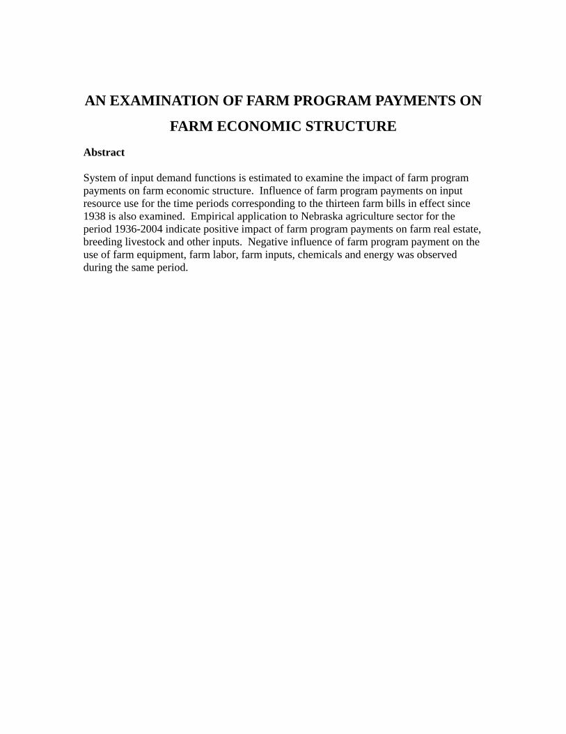
Abstract

System of input demand functions is estimated to examine the impact of farm program payments on farm economic structure. Influence of farm program payments on input resource use for the time periods corresponding to the thirteen farm bills in effect since 1938 is also examined. Empirical application to Nebraska agriculture sector for the period 1936-2004 indicate positive impact of farm program payments on farm real estate, breeding livestock and other inputs. Negative influence of farm program payment on the use of farm equipment, farm labor, farm inputs, chemicals and energy was observed during the same period.

AN EXAMINATION OF FARM PROGRAM PAYMENTS

ON FARM ECONOMIC STRUCTURE

Farm commodity programs, once viewed as temporary and supplementary to

agricultural earnings, are increasingly viewed as permanent and of major proportion.

Existing literature has examined numerous aspects of agricultural policy including

whether farm program payments - have enhanced land owner wealth rather than the

welfare of producers; have altered the crop mix; or influenced trade distortions.

Recent analyses have also examined the impact of different kinds of program

payments on specific crop or region. With the 2007 farm bill discussions concluding,

farm program payments have become much more important as a farm policy

instrument. While the causes of the switch to different kinds of program are still

controversial, as are the predicted outcomes, there is strong interest in the potential

effects of farm program payments on farm economic structure.

Current research had addressed crop- and input-specific effects of program

payments on farm economic structure, including adverse selection, moral hazard,

demand, and the potential environmental and trade effects. This line of research is

appropriate and relevant due to the current setting of programs that is crop specific.

However, there is a need to examine the overall influence of farm program payments

on the resource use or output production mix to provide broader policy analyses and

implications. Here, the economic effects of farm program payments on farm

economic structure is examined with specific analysis on the farm equipment, farm

real estate, breeding livestock, farm inputs, chemicals, energy and other input demand

2

functions. Influence of farm program payments on input resource use for the time

periods corresponding to the thirteen farm bills in effect since 1938 is also examined.

With this analysis an important contribution from a policy perspective is the ability to

examine the potential impacts of farm program payments on the use of farm

equipment, farm real estate, breeding livestock, farm inputs, chemicals, energy and

other inputs. From our (Shaik et al) earlier analyses we know the positive impact of

farm program payments on farm real estate, so we expect to see a positive relation

between farm program payments and farm real estate demand. Others have examined

the moral hazard issue of circumventing and/or lowering the use of chemical

(fertilizers and pesticide use) due to the availability of farm program payments. This

would also provide the influence of farm program payments on energy use in

agriculture sector. Apart from the overall influence of farm program payments on

input resource use, we also examine the changes in the influence of farm program

payments on input resource use over the thirteen farm bill periods.

A farm bill refers to a multi-year, multi-commodity federal support law for

farm products. Some standing authority for these programs is provided by two

permanent laws, the Agricultural Adjustment Act of 1938 and the Agricultural Act of

1949. However, Congress usually amends these provisions, reauthorizes or amends

provisions of preceding temporary agricultural acts, and/or puts forth new provisions

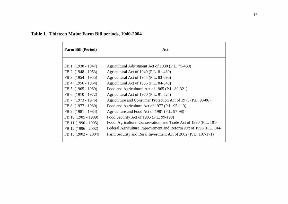
for a limited time into the future during the farm bill authorization process. Table 1

provides the chronology of major farm bills since 1938.

This paper has two-fold contribution to the existing literature - 1) construct the

output, input, and farm government payment Fisher quantity and price indexes for

Nebraska agriculture sector from 1936-2004, 2) examines the impact of farm program

3

payments on input resource use, and 3) examines the impact of farm program

payments by thirteen farm bill periods on input resource use in system of equations.

In the next section the econometric Translog system of input demand equations

(includes farm equipment, breeding livestock, farm real estate, farm inputs,

chemicals, energy and others) including farm program payments and its interaction by

farm bill period is presented. For this analysis Nebraska was specifically chosen due

to the availability of dis-aggregate output and input quantity and price data apart from

the farm program payment data. Construction of Nebraska agriculture sector input,

output and farm program payment data for the period, 1936-2004 is detailed in the

third section. Empirical application and results are presented in the fourth section

followed by conclusions.

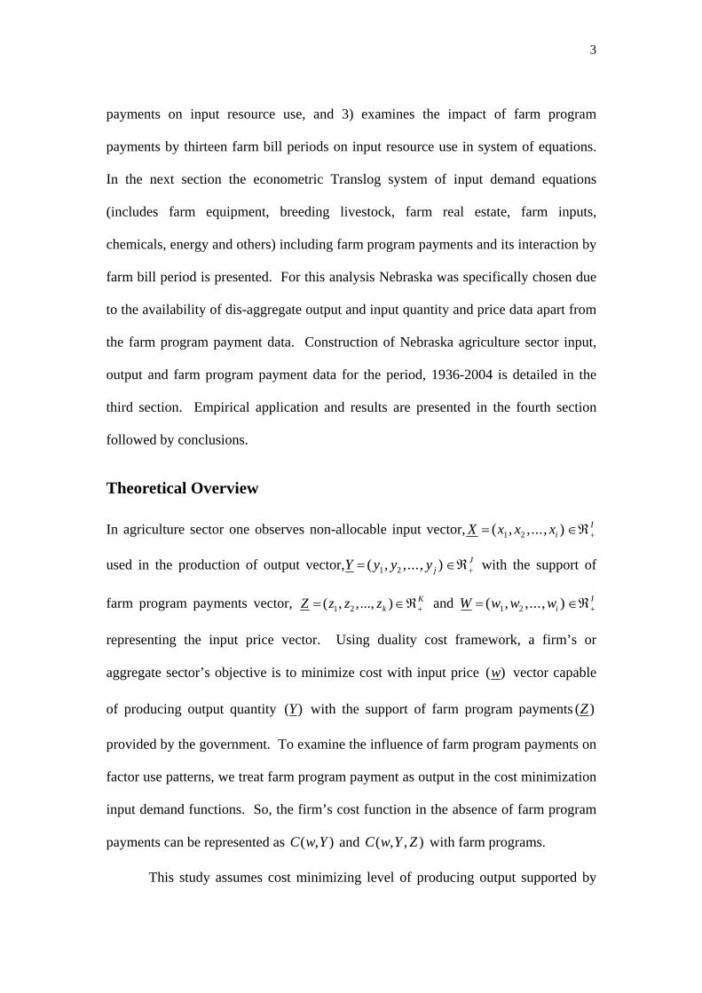
Theoretical Overview

In agriculture sector one observes non-allocable input vector, X x x xiI= ∈ℜ+( , ,..., )1 2

used in the production of output vector,Y y y y jJ= ∈ℜ+( , ,..., )1 2 with the support of

farm program payments vector, 1 2( , ,..., ) KkZ z z z += ∈ℜ and W w w wi

I= ∈ℜ+( , ,..., )1 2

representing the input price vector. Using duality cost framework, a firm’s or

aggregate sector’s objective is to minimize cost with input price ( )w vector capable

of producing output quantity ( )Y with the support of farm program payments ( )Z

provided by the government. To examine the influence of farm program payments on

factor use patterns, we treat farm program payment as output in the cost minimization

input demand functions. So, the firm’s cost function in the absence of farm program

payments can be represented as and with farm programs. ( , )C w Y ( , , )C w Y Z

This study assumes cost minimizing level of producing output supported by

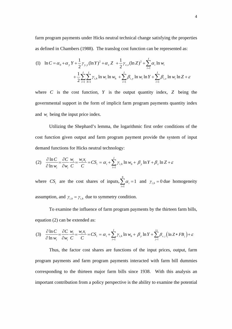
4

farm program payments under Hicks neutral technical change satisfying the properties

as defined in Chambers (1988). The translog cost function can be represented as:

2 20 , ,

1

, , ,1 1 1 1

1 1(1) ln (ln ) (ln ) ln2 21 ln ln ln ln ln ln2

I

y y y z z z i ii

I I I I

i h i h i y i i z ii h i i

C Y Y Z Z w

w w w Y w Z

α α γ α γ α

γ β β

=

= = = =

= + + + + +

+ + +

∑

∑∑ ∑ ∑ ε+

where is the cost function, Y is the output quantity index, C Z being the

governmental support in the form of implicit farm program payments quantity index

and being the input price index. iw

Utilizing the Shephard’s lemma, the logarithmic first order conditions of the

cost function given output and farm program payment provide the system of input

demand functions for Hicks neutral technology:

,1

ln(2) ln ln lnln

Ii i i

i i i h h y zii i

w w xC C CS w Y Zw w C C

α γ β β=

∂ ∂= = = = + + +

∂ ∂ ∑ ε+

where are the cost shares of inputs,iCS8

11i

iα

=

=∑ and , 0i hγ = due homogeneity

assumption, and ,i h i h,γ γ= due to symmetry condition.

To examine the influence of farm program payments by the thirteen farm bills,

equation (2) can be extended as:

( )13

,1

,1

lnln(3) ln lnln z j j

j

Ii i i

i i i h h yii i

Z FBw w xC C CS w Y

w w C Cβα γ β

==

∗∂ ∂

= = = = + + +∂ ∂ ∑∑ ε+

Thus, the factor cost shares are functions of the input prices, output, farm

program payments and farm program payments interacted with farm bill dummies

corresponding to the thirteen major farm bills since 1938. With this analysis an

important contribution from a policy perspective is the ability to examine the potential

5

impacts of farm program payments on the input resource use.

Nebraska Output, Input and Farm Program Payment Data1

The input, output and the farm program payment data for Nebraska agriculture span

from 1936 to 2004. Aggregate agricultural output, eight categories of inputs and an

aggregate farm program payment are computed and aggregated to be used in the

estimation of the model. Aggregated output quantity index is constructed from 23

commodities including 10 livestock commodities, 2 food grains and 6 feed crops and

5 oils and vegetable crops. Similarly eight aggregated input quantity indexes are also

constructed from 25 variables including 4 farm equipments, 4 farm real estate

including building and structures, 4 breeding livestock, 2 types of farm labor and 11

intermediate inputs. The aggregate farm program payment variable is constructed as

only aggregate level data is available from 1936-2004.

Outputs

Prices and quantity data were obtained from Nebraska Agriculture Statistics

Historical Record 1866-1954 and Unpublished Official Estimates sheet2 maintained

by the Nebraska Department of Agriculture. For later years data was obtained from

NASS website. Annual data on crop output is the quantity produced [yield per acre

times total harvested acres for each crop] during the crop year. Crop prices received

by farmers, as reported in annual Nebraska Agriculture Statistics were used in the

construction of output quantity index. The three aggregated crop quantity indexes are

1 Source of the input and output data is from “Statistical Appendix of Nebraska Outputs, Inputs and Environmental bads Data for Dissertation” of Shaik’s Dissertation titled “Environmentally Adjusted Productivity Measures for the Nebraska Agriculture Sector, 1936-1994”. 2Would like to thank Nebraska Agriculture Statistical Services for providing me with the data and also discussing the procedure in the estimation of the series.

6

food grains [rye and wheat], feed crops [barely, corn, hay, oats and sorghum] and

vegetable and oilseed crops [soybean, sunflower, dry bean, potatoes and sugar beet].

In 2004 these crops constitute 100% of the crop data published by Nebraska

Department of Agriculture for major and minor crops.

Similarly for livestock commodities, the quantity estimates [pounds of meat

produced (gained weight)] for cattle and calves, hogs, sheep & lambs, broilers, eggs,

turkeys, and chickens and the marketing year average prices per pound reported in

annual Nebraska Agriculture Statistics were used to construct the livestock quantity

indexes. The price and quantity data on milk, honey and wool output obtained from

Unpublished Official Estimates sheet was used in the construction of output quantity

index. For later years data was obtained from NASS website. The three livestock

output quantity indexes constructed are meat animal [cattle and calves, hogs, sheep

and lambs], poultry [chicken, broiler, eggs and turkey] and other [honey, wool and

milk production].

In case of feed grain and feed crops, part of the grains and feed are fed to

animals on the farm where it is grown. The question is whether to adjust the output

for onfarm use or add the additional cost of onfarm use as an intermediate input.

Based on AAEA recommendations included the feed crops consumed on the farm

along with purchased feeds as a measure of intermediate input. The gross production

of the feed grains is included as output, and if onfarm use were unaccounted for, the

result would be double counting of feed-once as crop production and again indirectly

in livestock production.

7

Inputs

In regards to inputs particular emphasis was given in the construction of capital3,

labor and intermediate inputs. To measure farm equipment4 contribution to

agriculture inputs, first we estimated the capital stock based on the annual capital

investment expenditures It series published by USDA, ERS internet electronic

database. Nebraska share of investments is obtained by multiplying the Nebraska/US

ratio of inventory of capital machinery by US investments for each of the four assets.

To obtain an implicit quantity index of capital goods purchased It’, It was divided by

the individual producer price index5 for various capital goods. This It’ gives a time

series of the quantity of capital goods purchased, expressed in terms of the cost that

would have been incurred under 2000 prices for the capital goods. The perpetual

inventory method was used to estimate the level of “capital stock” for four assets,

based on a straight-line depreciation pattern. Capital stock is calculated as the

weighted (relative efficiency) sum of the past investments.

(4) 0

( )t tK S I ττ

τ∞

−=

= ∑

where ( )S τ is the efficiency function, I is the expenditures and τ is the age of the

capital.

The efficiency function is assumed to be a function of mean service life (age)

in straight line depreciation pattern6 (1 over mean service life). The mean service life

3 Consists of Farm equipment, Farm real estate and Breeding livestock. 4 Consists of Autos, Trucks, Tractors & Agricultural Machinery except tractors. 5 USDA and Bureau of Labor Statistics publishes producer price index (PPI) annual for different components of capital equipment with base year T=2000 which is comparable to price index paid by the farmers. 6 Alternative depreciation patterns are also examined, but it did affect the results in the system of input demand functions.

8

(L), are the Bureau of Economics Analysis [BEA] estimates obtained from Fixed

Reproducible Tangible Wealth in the United States (1993).

The “rental value” or “user cost” of capital is based on the neoclassical

principle that inputs should be aggregated using weights that reflect their marginal

products which is estimated in terms of rental value. The rental value is calculated as:

(5) ( )t tRV K r δ= +

where RV is the rental value, is the capital stock, r is the real interest rate and tK

δ is the depreciation.

The straight-line deprecation value is estimated for the different class of asset

as one over 0.98 times life service of 9, 10, 9 and 14 for trucks, autos, tractor and

agricultural machinery excluding tractors respectively. Rental value is used to

calculate shares to form a farm equipment quantity index.

In the case of farm real estate7 we disaggregate into three types of land (non-

irrigated cropland, irrigated cropland and pasture land) apart from building and

structures to be used in constructing of farm real estate quantity index. The cash

rents8 for the three categories are available from 1971 onwards, but for data prior to

1971 cash rents were available only for pastures and cropland. So farm cropland cash

rent was used to extrapolate backwards for irrigated and non-irrigated land. Here idle

cropland is excluded from the number of acres nonirrigated cropland, since from the

perspective of agriculture productivity we need to account only for that land used in

agriculture. The annual series was constructed by interpolating between the census

7 Consist of three types of land, i.e., Irrigated, Non-irrigated and Pastures apart from farm structures. 8 I would like to thank Dr. Charles Barnard and Dr. John Jones from USDA for kindly providing unpublished data on the historical cash rents.

9

years. In the case of nonirrigated cropland the interpolation between the census years

was based on the regional data published in USDA, ECIFS (1990). The period

covered by this report is from 1947-90 and for more current data, AREI, ERS and

NASS updates are used. By disaggregating land, we hope to adjust for the changes in

the quantity and quality of land in agriculture. Cash rents are used to calculate shares

to form a quantity land index. In the case of building and structures the current value

of building is published by Jones and Canning (1993). With the recent data provided

by computer file update on USDA, ERS internet database. Data prior to 1950 was

obtained from Nebraska Agriculture Statistics Historical Record 1866-1954. This is

used as a measure of capital stock and rental value is calculated following the same

procedure as farm equipment with a 35 year life. The rental value is calculated to

form a farm real estate quantity index.

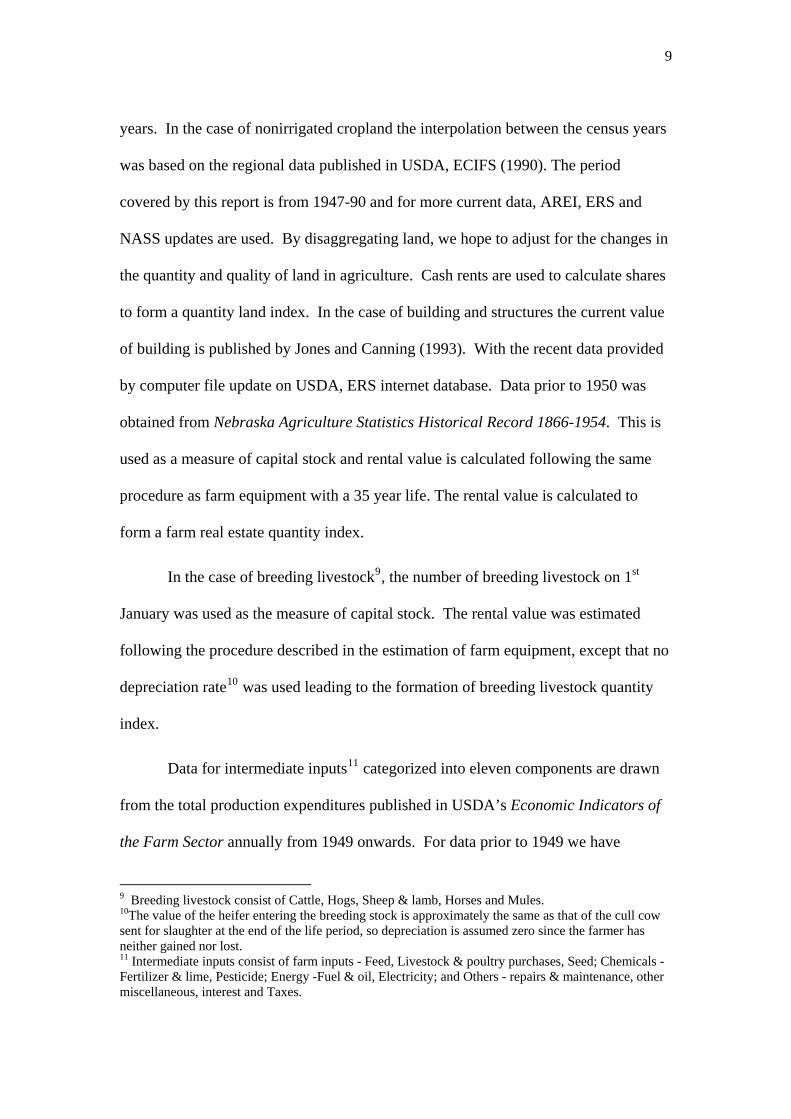
In the case of breeding livestock9, the number of breeding livestock on 1st

January was used as the measure of capital stock. The rental value was estimated

following the procedure described in the estimation of farm equipment, except that no

depreciation rate10 was used leading to the formation of breeding livestock quantity

index.

Data for intermediate inputs11 categorized into eleven components are drawn

from the total production expenditures published in USDA’s Economic Indicators of

the Farm Sector annually from 1949 onwards. For data prior to 1949 we have

9 Breeding livestock consist of Cattle, Hogs, Sheep & lamb, Horses and Mules. 10The value of the heifer entering the breeding stock is approximately the same as that of the cull cow sent for slaughter at the end of the life period, so depreciation is assumed zero since the farmer has neither gained nor lost. 11 Intermediate inputs consist of farm inputs - Feed, Livestock & poultry purchases, Seed; Chemicals - Fertilizer & lime, Pesticide; Energy -Fuel & oil, Electricity; and Others - repairs & maintenance, other miscellaneous, interest and Taxes.

10

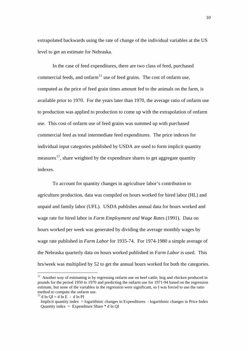
extrapolated backwards using the rate of change of the individual variables at the US

level to get an estimate for Nebraska.

In the case of feed expenditures, there are two class of feed, purchased

commercial feeds, and onfarm12 use of feed grains. The cost of onfarm use,

computed as the price of feed grain times amount fed to the animals on the farm, is

available prior to 1970. For the years later than 1970, the average ratio of onfarm use

to production was applied to production to come up with the extrapolation of onfarm

use. This cost of onfarm use of feed grains was summed up with purchased

commercial feed as total intermediate feed expenditures. The price indexes for

individual input categories published by USDA are used to form implicit quantity

measures13, share weighted by the expenditure shares to get aggregate quantity

indexes.

To account for quantity changes in agriculture labor’s contribution to

agriculture production, data was compiled on hours worked for hired labor (HL) and

unpaid and family labor (UFL). USDA publishes annual data for hours worked and

wage rate for hired labor in Farm Employment and Wage Rates (1991). Data on

hours worked per week was generated by dividing the average monthly wages by

wage rate published in Farm Labor for 1935-74. For 1974-1980 a simple average of

the Nebraska quarterly data on hours worked published in Farm Labor is used. This

hrs/week was multiplied by 52 to get the annual hours worked for both the categories.

12 Another way of estimating is by regressing onfarm use on beef cattle, hog and chicken produced in pounds for the period 1950 to 1970 and predicting the onfarm use for 1971-94 based on the regression estimate, but none of the variables in the regression were significant, so I was forced to use the ratio method to compute the onfarm use. 13 d ln QI = d ln E - d ln PI Implicit quantity index = logarithmic changes in Expenditures - logarithmic changes in Price Index Quantity index = Expenditure Share * d ln QI

11

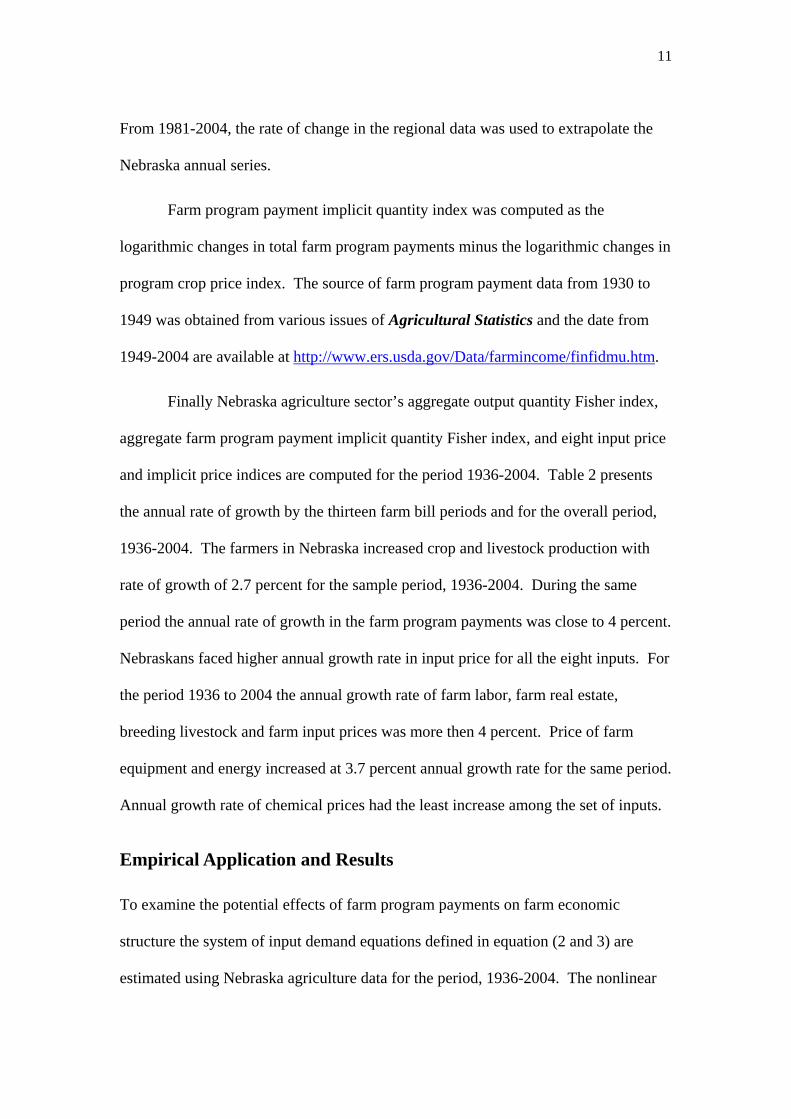
From 1981-2004, the rate of change in the regional data was used to extrapolate the

Nebraska annual series.

Farm program payment implicit quantity index was computed as the

logarithmic changes in total farm program payments minus the logarithmic changes in

program crop price index. The source of farm program payment data from 1930 to

1949 was obtained from various issues of Agricultural Statistics and the date from

1949-2004 are available at http://www.ers.usda.gov/Data/farmincome/finfidmu.htm.

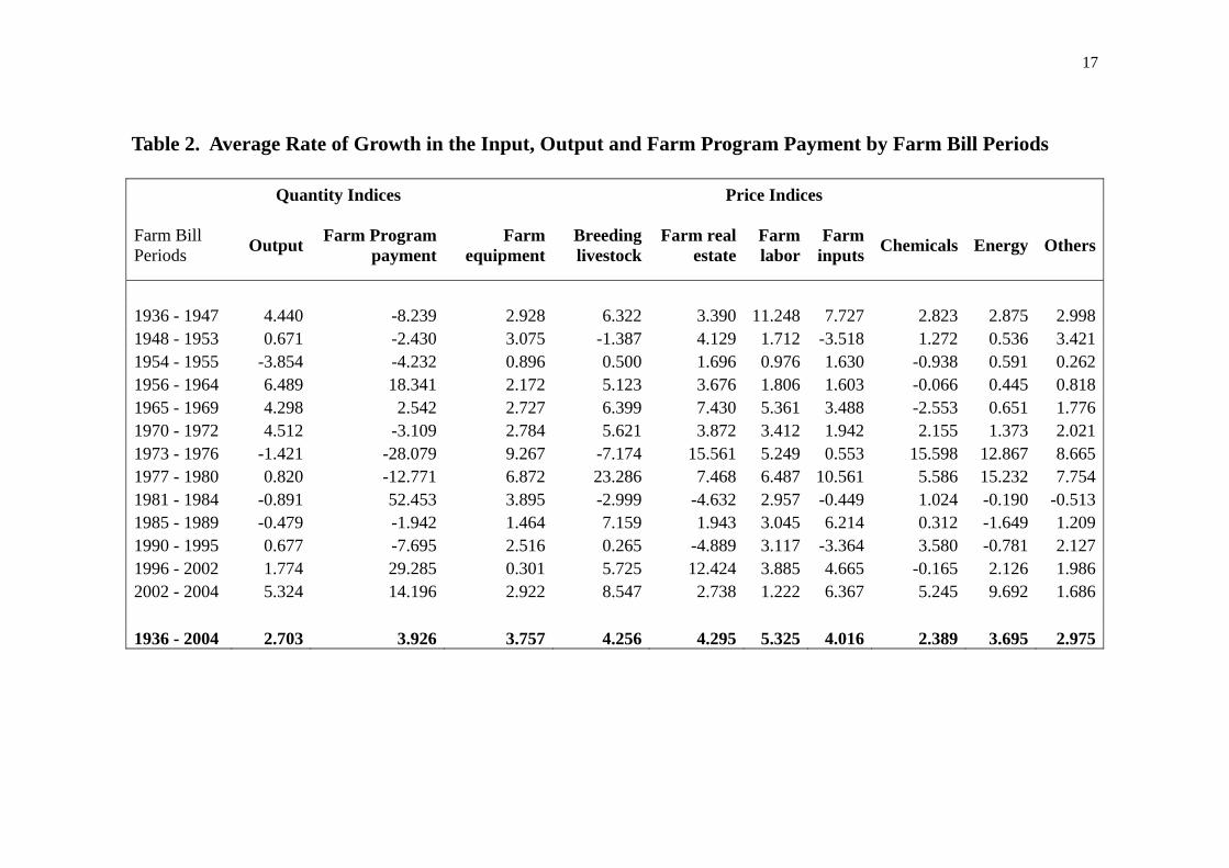
Finally Nebraska agriculture sector’s aggregate output quantity Fisher index,

aggregate farm program payment implicit quantity Fisher index, and eight input price

and implicit price indices are computed for the period 1936-2004. Table 2 presents

the annual rate of growth by the thirteen farm bill periods and for the overall period,

1936-2004. The farmers in Nebraska increased crop and livestock production with

rate of growth of 2.7 percent for the sample period, 1936-2004. During the same

period the annual rate of growth in the farm program payments was close to 4 percent.

Nebraskans faced higher annual growth rate in input price for all the eight inputs. For

the period 1936 to 2004 the annual growth rate of farm labor, farm real estate,

breeding livestock and farm input prices was more then 4 percent. Price of farm

equipment and energy increased at 3.7 percent annual growth rate for the same period.

Annual growth rate of chemical prices had the least increase among the set of inputs.

Empirical Application and Results

To examine the potential effects of farm program payments on farm economic

structure the system of input demand equations defined in equation (2 and 3) are

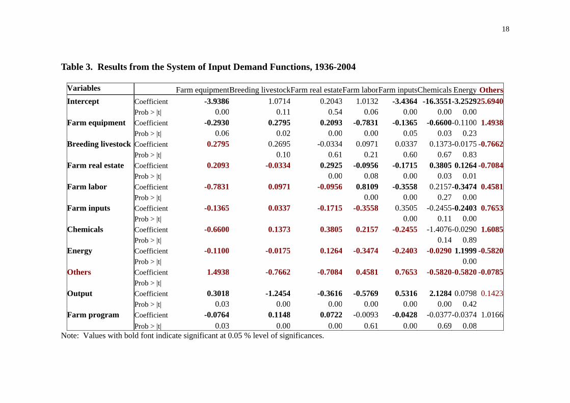
estimated using Nebraska agriculture data for the period, 1936-2004. The nonlinear

12

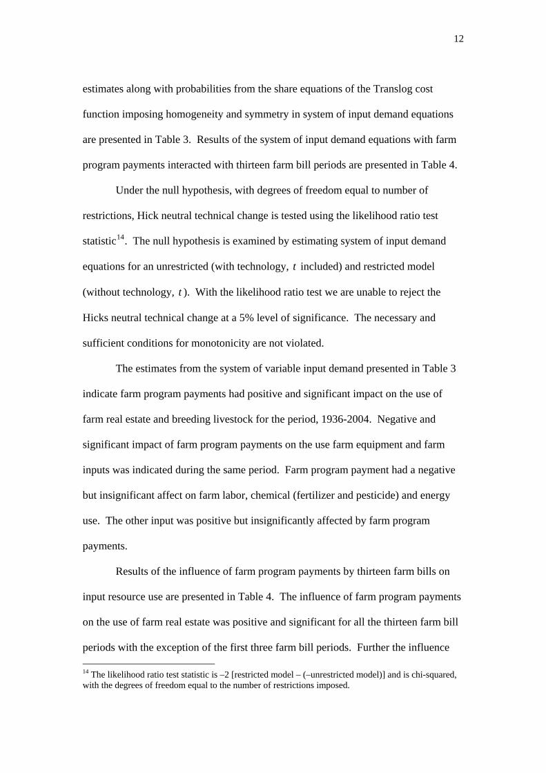
estimates along with probabilities from the share equations of the Translog cost

function imposing homogeneity and symmetry in system of input demand equations

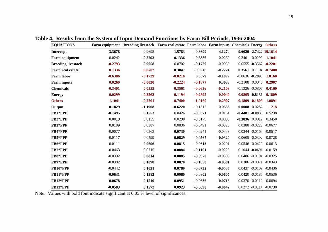
are presented in Table 3. Results of the system of input demand equations with farm

program payments interacted with thirteen farm bill periods are presented in Table 4.

Under the null hypothesis, with degrees of freedom equal to number of

restrictions, Hick neutral technical change is tested using the likelihood ratio test

statistic14. The null hypothesis is examined by estimating system of input demand

equations for an unrestricted (with technology, included) and restricted model

(without technology, ). With the likelihood ratio test we are unable to reject the

Hicks neutral technical change at a 5% level of significance. The necessary and

sufficient conditions for monotonicity are not violated.

t

t

The estimates from the system of variable input demand presented in Table 3

indicate farm program payments had positive and significant impact on the use of

farm real estate and breeding livestock for the period, 1936-2004. Negative and

significant impact of farm program payments on the use farm equipment and farm

inputs was indicated during the same period. Farm program payment had a negative

but insignificant affect on farm labor, chemical (fertilizer and pesticide) and energy

use. The other input was positive but insignificantly affected by farm program

payments.

Results of the influence of farm program payments by thirteen farm bills on

input resource use are presented in Table 4. The influence of farm program payments

on the use of farm real estate was positive and significant for all the thirteen farm bill

periods with the exception of the first three farm bill periods. Further the influence 14 The likelihood ratio test statistic is –2 [restricted model – (–unrestricted model)] and is chi-squared, with the degrees of freedom equal to the number of restrictions imposed.

13

increased from the fourth farm bill period onwards to the current farm bill period. A

similar increasing and significant influence of farm program payments on the use of

breeding livestock was indicated from the sixth farm bill period to the current farm

bill period, 2002-2004. Farm program payments had a negative influence on the use

of farm equipment with the exception of the second and third farm bill period. While

farm program payment was significant during the recent three farm bill periods. The

lower use of farm labor in agriculture was also supported by the farm program

payments for all the thirteen farm bill periods. The influence was significant and

significant from the fifth farm bill period onwards to the current farm bill period.

Farm program payment had reduced the use of chemicals (fertilizer and pesticide)

only during the first two farm bill periods, but was positive and insignificant third

farm bill period onwards. At the aggregate level this result suggests the absence of

moral hazard i.e., producer do not lower the use of chemicals due to the presence of

farm program payments. The remaining variables including energy use and other

input use was negative but insignificant.

Overall the empirical state level analysis of Nebraska agriculture sector

indicates potential impacts of farm program payments on the farm economic structure.

This is based on the estimation of input demand functions accounting for farm

program payments variable. A more through investigation of the model as well as

estimation procedure would provide clear and robust impacts due to farm program

payment on factor use. Further simultaneous estimation of system of input demand

and output supply equations along with the profit function would provide the detailed

impact analysis of the potential impacts of farm program payment on the factor use as

well as shifts in the crop production mix.

14

Conclusions

This paper examines the potential impacts of farm program payments on Nebraska

agriculture sector based on the system of input demand equations using a cost

function for the time period 1936-2004. The likelihood ratio tests fail to accept the

non-Hick-neutral technical change. So under Hicks-neutral technical change, the

overall impacts of farm program payment on agriculture sector based on the system of

input demand equations indicate positive (negative) and significant sign on the farm

real estate, breeding livestock and other inputs (farm equipment, farm labor, farm

inputs, chemicals and energy) for the period 1936-2004. Similar sign on the input

resource use was indicated with the exception of chemical use over the thirteen farm

bill periods. However, there is increasing and decreasing influence of farm program

payments over the farm bill period for the positive and negative sign on the variables

respectively.

Further research needs to be explored on the consistency of estimate by testing

for unit root/cointegration and accounting for unit roots if any; examine the impact of

farm program payment based on the system of input demand and output supply

equations.

15

References

Chambers, R.G. “Insurability and Moral Hazard in Agricultural Insurance Markets.” American Journal of Agricultural Economics. 71(1989): 604-16.

Nebraska Department of Agriculture., and United States Department of Agriculture, NASS. “Nebraska Agricultural Statistics,” Annual Report. Nebraska Crop and Livestock Reporting Service, Nebraska.

Nebraska Department of Agriculture and Inspection., and United States Department of Agriculture. “Nebraska Agriculture Statistics: Historical Record, 1866-1954,” State-Federal Division of Agricultural Statistics, Nebraska 1956.

Shaik, S. “Environmentally Adjusted Productivity [EAP] Measures for Nebraska Agriculture Sector” Dissertation, Dept. of Agriculture Economics, University of Nebraska-Lincoln, May 1998.

Shaik, S, G. A. Helmers, and J.A.Atwood. “Government Payments and Agricultural Land Values.” Mississippi State University Department of Agricultural Economics Staff Report 2005-02, February 2005.

Shaik, S, J.A.Atwood and G. A. Helmers. “The Evolution of Farm Programs and their Contribution to Agricultural Land Values” American Journal of Agricultural Economics, 87 (2005): 1190-1197.

U.S. Crop Reporting Board. Commercial Fertilizers: Annual Summary, Dept. of Agriculture, Economics, Statistics, and Cooperative Service.

U.S. Department of Agriculture. Agricultural Statistics Annual, Washington, D.C. Department of Agriculture, U.S. Govt. Print. Office.

U.S. Department of Agriculture, National Agricultural Statistical Service. “Farm Employment and Wages, 1910-1990.” Statistical Bulletin N0. 822, March 1991.

U.S. Department of Agriculture. Crop Reporting Board, Statistical Service. “Farm Labor.” Annual reports.

U.S. Department of Agriculture, National Agricultural Statistical Service. “Agricultural Chemical Usage, Field Crop Summary.” Annual reports, 1991-1994.

U.S. Department of Agriculture. “Economic Indicators of the Farm Sector, National Financial Summary.” Economic Research Service, ECIFS 4-3 , 1989.

U.S. Department of Agriculture. “Economic Indicators of the Farm Sector, Production and Efficiency Statistics.” Economic Research Service, ECIFS 10-3, 1990.(May 1992).

U.S. Department of Commerce. “Fixed Reproducible Tangible Wealth in the United States, 1925–89.” Washington DC: U.S. Government Printing Office, 1993.

16

Table 1. Thirteen Major Farm Bill periods, 1940-2004

Farm Bill (Period) Act FB 1 (1938 - 1947) Agricultural Adjustment Act of 1938 (P.L. 75-430) FB 2 (1948 - 1953) Agricultural Act of 1949 (P.L. 81-439) FB 3 (1954 - 1955) Agricultural Act of 1954 (P.L. 83-690) FB 4 (1956 - 1964) Agricultural Act of 1956 (P.L. 84-540) FB 5 (1965 - 1969) Food and Agricultural Act of 1965 (P.L. 89-321) FB 6 (1970 - 1972) Agricultural Act of 1970 (P.L. 91-524) FB 7 (1973 - 1976) Agriculture and Consumer Protection Act of 1973 (P.L. 93-86) FB 8 (1977 - 1980) Food and Agriculture Act of 1977 (P.L. 95-113) FB 9 (1981 - 1984) Agriculture and Food Act of 1981 (P.L. 97-98) FB 10 (1985 - 1989) Food Security Act of 1985 (P.L. 99-198) FB 11 (1990 - 1995) Food, Agriculture, Conservation, and Trade Act of 1990 (P.L. 101-

)FB 12 (1996 - 2002) Federal Agriculture Improvement and Reform Act of 1996 (P.L. 104-)FB 13 (2002 - 2004) Farm Security and Rural Investment Act of 2002 (P. L. 107-171)

17

Table 2. Average Rate of Growth in the Input, Output and Farm Program Payment by Farm Bill Periods

Quantity Indices Price Indices

Farm Bill Periods Output Farm Program

paymentFarm

equipmentBreeding livestock

Farm real estate

Farm labor

Farm inputs Chemicals Energy Others

1936 - 1947 4.440 -8.239 2.928 6.322 3.390 11.248 7.727 2.823 2.875 2.998 1948 - 1953 0.671 -2.430 3.075 -1.387 4.129 1.712 -3.518 1.272 0.536 3.421 1954 - 1955 -3.854 -4.232 0.896 0.500 1.696 0.976 1.630 -0.938 0.591 0.262 1956 - 1964 6.489 18.341 2.172 5.123 3.676 1.806 1.603 -0.066 0.445 0.818 1965 - 1969 4.298 2.542 2.727 6.399 7.430 5.361 3.488 -2.553 0.651 1.776 1970 - 1972 4.512 -3.109 2.784 5.621 3.872 3.412 1.942 2.155 1.373 2.021 1973 - 1976 -1.421 -28.079 9.267 -7.174 15.561 5.249 0.553 15.598 12.867 8.665 1977 - 1980 0.820 -12.771 6.872 23.286 7.468 6.487 10.561 5.586 15.232 7.754 1981 - 1984 -0.891 52.453 3.895 -2.999 -4.632 2.957 -0.449 1.024 -0.190 -0.513 1985 - 1989 -0.479 -1.942 1.464 7.159 1.943 3.045 6.214 0.312 -1.649 1.209 1990 - 1995 0.677 -7.695 2.516 0.265 -4.889 3.117 -3.364 3.580 -0.781 2.127 1996 - 2002 1.774 29.285 0.301 5.725 12.424 3.885 4.665 -0.165 2.126 1.986 2002 - 2004 5.324 14.196 2.922 8.547 2.738 1.222 6.367 5.245 9.692 1.686 1936 - 2004 2.703 3.926 3.757 4.256 4.295 5.325 4.016 2.389 3.695 2.975

18

Table 3. Results from the System of Input Demand Functions, 1936-2004

Variables Farm equipmentBreeding livestockFarm real estateFarm laborFarm inputsChemicals Energy OthersIntercept Coefficient -3.9386 1.0714 0.2043 1.0132 -3.4364 -16.3551-3.252925.6940 Prob > |t| 0.00 0.11 0.54 0.06 0.00 0.00 0.00 Farm equipment Coefficient -0.2930 0.2795 0.2093 -0.7831 -0.1365 -0.6600-0.1100 1.4938 Prob > |t| 0.06 0.02 0.00 0.00 0.05 0.03 0.23 Breeding livestock Coefficient 0.2795 0.2695 -0.0334 0.0971 0.0337 0.1373-0.0175 -0.7662 Prob > |t| 0.10 0.61 0.21 0.60 0.67 0.83 Farm real estate Coefficient 0.2093 -0.0334 0.2925 -0.0956 -0.1715 0.3805 0.1264 -0.7084 Prob > |t| 0.00 0.08 0.00 0.03 0.01 Farm labor Coefficient -0.7831 0.0971 -0.0956 0.8109 -0.3558 0.2157-0.3474 0.4581 Prob > |t| 0.00 0.00 0.27 0.00 Farm inputs Coefficient -0.1365 0.0337 -0.1715 -0.3558 0.3505 -0.2455-0.2403 0.7653 Prob > |t| 0.00 0.11 0.00 Chemicals Coefficient -0.6600 0.1373 0.3805 0.2157 -0.2455 -1.4076-0.0290 1.6085 Prob > |t| 0.14 0.89 Energy Coefficient -0.1100 -0.0175 0.1264 -0.3474 -0.2403 -0.0290 1.1999 -0.5820 Prob > |t| 0.00 Others Coefficient 1.4938 -0.7662 -0.7084 0.4581 0.7653 -0.5820-0.5820 -0.0785 Prob > |t| Output Coefficient 0.3018 -1.2454 -0.3616 -0.5769 0.5316 2.1284 0.0798 0.1423 Prob > |t| 0.03 0.00 0.00 0.00 0.00 0.00 0.42 Farm program Coefficient -0.0764 0.1148 0.0722 -0.0093 -0.0428 -0.0377-0.0374 1.0166 Prob > |t| 0.03 0.00 0.00 0.61 0.00 0.69 0.08

Note: Values with bold font indicate significant at 0.05 % level of significances.

19

Table 4. Results from the System of Input Demand Functions by Farm Bill Periods, 1936-2004 EQUATIONS Farm equipment Breeding livestock Farm real estate Farm labor Farm inputs Chemicals Energy Others

Intercept -3.3678 0.9695 1.5783 -0.8699 -4.1274 -9.6020 -2.7422 19.1614Farm equipment 0.0242 -0.2793 0.1336 -0.6386 0.0260 -0.3401 -0.0299 1.1041Breeding livestock -0.2793 0.9058 0.0702 -0.1729 -0.0030 0.0555 -0.3562 -0.2201Farm real estate 0.1336 0.0702 0.3047 -0.0216 -0.2224 0.3561 0.1194 -0.7400Farm labor -0.6386 -0.1729 -0.0216 0.3579 -0.1877 -0.0636 -0.2895 1.0160Farm inputs 0.0260 -0.0030 -0.2224 -0.1877 0.3033 -0.2108 0.0040 0.2907Chemicals -0.3401 0.0555 0.3561 -0.0636 -0.2108 -0.1326 -0.0805 0.4160Energy -0.0299 -0.3562 0.1194 -0.2895 0.0040 -0.0805 0.8136 -0.1809Others 1.1041 -0.2201 -0.7400 1.0160 0.2907 -0.1809 -0.1809 -1.0891Output 0.1829 -1.1908 -0.6220 -0.1312 -0.0636 0.0008 -0.0252 1.1218FB1*FPP -0.1495 0.1553 0.0426 -0.0571 0.0164 -0.4481 -0.0833 0.5238FB2*FPP 0.0019 0.0155 0.0290 -0.0179 0.0088 -0.3836 0.0012 0.3450FB3*FPP 0.0109 0.0387 0.0836 -0.0491 -0.0328 0.0388 -0.0223 -0.0677FB4*FPP -0.0077 0.0363 0.0730 -0.0241 -0.0339 0.0344 -0.0163 -0.0617FB5*FPP -0.0117 0.0599 0.0829 -0.0567 -0.0320 0.0605 -0.0302 -0.0728FB6*FPP -0.0111 0.0696 0.0815 -0.0613 -0.0291 0.0546 -0.0429 -0.0613FB7*FPP -0.0463 0.0715 0.0884 -0.1101 -0.0225 0.1044 -0.0696 -0.0159FB8*FPP -0.0392 0.0814 0.0885 -0.0970 -0.0395 0.0486 -0.0104 -0.0325FB9*FPP -0.0382 0.1098 0.0870 -0.1058 -0.0501 0.0386 -0.0071 -0.0343FB10*FPP -0.0442 0.1031 0.0789 -0.0732 -0.0537 0.0437 -0.0109 -0.0436FB11*FPP -0.0631 0.1382 0.0960 -0.0802 -0.0607 0.0420 -0.0187 -0.0536FB12*FPP -0.0678 0.1510 0.0951 -0.0636 -0.0713 0.0370 -0.0110 -0.0694

FB13*FPP -0.0583 0.1572 0.0923 -0.0698 -0.0642 0.0272 -0.0114 -0.0730Note: Values with bold font indicate significant at 0.05 % level of significances.