Surface Wind Regionalization in Complex Terrain

P. A. JIMÉNEZ,* J. F. GONZÁLEZ-ROUCO,� J. P. MONTÁVEZ,# J. NAVARRO,@

E. GARCÍA-BUSTAMANTE,* AND F. VALERO�

*División de Energías Renovables, CIEMAT, and Departamento de Astrofísica y Ciencias de la Atmósfera, UniversidadComplutense de Madrid, Madrid, Spain

�Departamento de Astrofísica y Ciencias de la Atmósfera, Universidad Complutense de Madrid, Madrid, Spain#Departamento de Física, Universidad de Murcia, Murcia, Spain

@División de Energías Renovables, CIEMAT, Madrid, Spain

(Manuscript received 25 April 2006, in final form 9 May 2007)

ABSTRACT

Daily wind variability in the Comunidad Foral de Navarra in northern Spain was studied using windobservations at 35 locations to derive subregions with homogeneous temporal variability. Two differentmethodologies based on principal component analysis were used to regionalize: 1) cluster analysis and 2) therotation of the selected principal components. Both methodologies produce similar results and lead toregions that are in general agreement with the topographic features of the terrain. The meridional windvariability is similar in all subregions, whereas zonal wind variability is responsible for differences betweenthem. The spectral analysis of wind variability within each subregion reveals a dominant annual cycle andthe varying presence of higher-frequency contributions in the subregions. The valley subregions tend topresent more variability at high frequencies than do higher-altitude sites. Last, the influence of large-scaledynamics on regional wind variability is explored by studying connections between wind in each subregionand sea level pressure fields. The results of this work contribute to the characterization of wind variabilityin a complex terrain region and constitute a framework for the validation of mesoscale model wind simu-lations over the region.

1. Introduction

Understanding and forecasting regional wind vari-ability is relevant for a wide variety of phenomena, forexample, the transport and dispersion of pollutantsalong an area, planning and decision making withinsituations of risk assessment related to the occurrenceof extreme events such as forest fires or structural dam-age, and power forecasting in wind farms. The latter isbecoming an issue with increasing demand for estab-lishing national policies in view of the recent develop-ments of renewable energy technologies.

Regional variability is controlled by the interactionof large-scale dynamics and orography. Circulation inthe free atmosphere is governed by gradients betweenthe large pressure systems. In the lower troposphere,the topography gains importance, generating a dynami-

cal forcing that modifies the direction and intensity ofwinds resulting from channeling, forced ascents, andbarrier effects (Whiteman 2000). These dynamicallydriven circulations show variations within the frequen-cies of a few days. In addition, differential heating andcooling of the soil drive local thermal circulations (Blu-men 1990), which depend on the temperature differ-ences along the valley axis or the mountain plains sys-tems, leading to diurnal frequency variations in re-sponse to the solar heating (Whiteman 2000).

Wind variability, therefore, is more complicated incomplex terrain regions where dynamically and ther-mally driven wind systems and their interactions gen-erate a wide variety of flow patterns (McGowan andSturman 1996). Furthermore, thermally driven winds atthe large scale can overwhelm those at the local scale asshown by Stewart et al. (2002) in their study of fourregions in western United States. The relationship be-tween the synoptic scale and the flow within a valleywas studied by Whiteman and Doran (1993), who sug-gested that the thermal forcing occurs when the large-scale dynamical forcing is weak. Because the dynami-

Corresponding author address: J. Fidel González-Rouco, Fac-ultad de Ciencias Fı́sicas, Universidad Complutense de Madrid,Avd. Complutense s/n, Madrid 28040, Spain.E-mail: fidelgr@fis.ucm.es

308 J O U R N A L O F A P P L I E D M E T E O R O L O G Y A N D C L I M A T O L O G Y VOLUME 47

DOI: 10.1175/2007JAMC1483.1

© 2008 American Meteorological Society

JAM2614

cally driven circulations are controlled by the synoptic-scale motions and the thermally driven circulationsbecome more relevant when these motions are weak,synoptic-scale motions either directly or indirectly con-trol the circulations over the surface. Their typical syn-optic variability of a few days makes it suitable to un-dertake a daily wind study.

The complicated circulations over complex terrainregions can be better understood by dividing the areainto a small number of internally homogeneous subre-gions, by means of a wind regionalization. One strategyto obtain areas of distinct regional behavior is to useeigenvector techniques. These techniques have beensuccessfully applied in a variety of case studies and forseveral variables (Dyer 1975; Bärring 1988; Stooksburyand Michaels 1991; Bonell and Sumner 1992; Fovell andFovell 1993; Comrie and Glenn 1998; Romero et al.1999a). However, the potential of the regionalizationapproach seldom has been explored with wind-relatedvariables (Cheng 1998). Regionalization of climate pa-rameters over a specific area contributes to the im-provement of the understanding of the spatial and tem-poral variability of the climate variable, and also offersa framework for the validation of mesoscale modelsimulations over the region (Romero et al. 1999a;Sotillo et al. 2003). Mesoscale models have become astandard tool for providing simulations and forecasts ofairflows in complex terrain regions, favored by recentincreases in computational power and accessibility ofanalysis and forecast grids (Mass and Kuo 1998). Anincreased understanding of wind variability provides abetter validation of mesoscale simulations (Rife et al.2004), and consequently the improvement of their ac-curacy. Regionalization allows for the establishment ofsubregions of distinct behavior in observations thatshould be reproduced by mesoscale models, thus offer-ing the possibility for designing model configurationsand test sensitivities either to initial and boundary con-ditions or to different physical parameterizations. Themodel evaluation at various identified subregions, in-stead of a point-to-point approach, that is, at specificgrid points or sites, allows the influence of local effectsthat are not usually modeled to be mitigated (vonStorch 1995).

This paper addresses the problem of wind regional-ization in a complex terrain region at daily time scales.Two different methods based on principal componentanalysis (PCA) are used. The first method carries outcluster analysis (CA) of the most important PCAmodes (Romero et al. 1999b), which allows for theidentification of homogeneous wind climate variabilitygroups, while the second method makes use of the ro-tation of selected principal components (White et al.

1991). The temporal variability of wind in each subre-gion is investigated by analyzing the spectra of the se-lected principal components. The Comunidad Foral deNavarra (CFN) region in northern Spain was selectedas the case study (Fig. 1) for this purpose. Its complextopography and strong wind conditions, which have re-sulted in increases of wind farm facilities in recenttimes, make it an interesting place to study wind vari-ability. The CFN region presents a complicated, highlyvariable topography with numerous valleys and moun-tain ridges that produce an interesting degree of inter-action with large-scale dynamics (Fig. 1), thus consti-tuting a useful case both for improving our understand-ing of wind variability at regional scales and for futureapplication in validation assessments of model perfor-mance.

This paper is organized as follows: Sections 2 and 3briefly describe the datasets and the multivariate meth-ods used in the regionalization process. Section 4 de-scribes results obtained from the CA and the PCA ro-tation-based approaches and further illustrates aspectsof the temporal wind variability in each region. Con-clusions and a discussion are presented in section 5.

2. Data

The location of the CFN in the north of the IberianPeninsula is highlighted in Fig. 1. The orography of theregion shows a variety of rich features broadly limitedby two large mountain systems: the Iberic System in thesouth of the CFN and the Pyrenees in the north, whichmerge westward with the last foothills of the Can-tabrian Mountains. Between them, the Ebro Valleycrosses the region from northwest to southeast towardthe Mediterranean. A closer look at the CFN (see en-larged area in Fig. 1) reveals a complex array of smallermountain systems and valleys. The north is dominatedby the Pyrenees, with the large Bidasoa mountain linesor the smaller sierras of Abodi, Uztarroz, San Miguel,Zariquieta, and Leyre. To simplify, the latter will bereferred to as the northern mountains. The western andnorthwestern boundaries are outflanked by the Aralarmountain lines as well as Urbasa, Santiago, and Andía,which will be herein labeled as western mountains, un-less treated specifically. The center and eastern side ofthe CFN is punctuated by the mountains systems ofIzco, San Pedro, and the Ujué peak, which will be la-beled as the eastern mountains. Last, the south of theCFN is dominated by the lower lands of the Ebro Val-ley. Virtually parallel to the Ebro Valley, smaller val-leys line up in the northwest–southeast direction southof the northern mountains. Similarly, west and east ofthe eastern mountain group, several mountain systems

JANUARY 2008 J I M É N E Z E T A L . 309

and valleys seem to favor wind channeling in the north-west–southeast and north–south directions. It will beillustrated that this is a major feature of the variabilityof the wind field within the region.

The dataset spans the period from 1 January 1992 to30 September 2002. The best 35 stations with the best-quality wind measurements from the meteorologicalnetwork of the CFN were selected for this study (Fig. 1,Table 1). Observations of wind speed and directionwere recorded at a height of 10 m above ground level,with the exception of seven stations in which the mea-surements were taken at 2 m, and with a time resolutionof 10 min (Table 1).

These initial data were quality controlled by applyingvarious tests that are similar to those employed in otherquality control analysis (Meek and Hatfield 1994; De-Gaetano 1997; Graybeal 2006). In particular, severaltests were applied to identify and eliminate errors ofsensor or data manipulation (repetition, unrealisticallyhigh or low values, etc.), to invalidate abnormally high-or low-variability periods in order to ensure temporalconsistency, as well as to assess the long-term variabil-ity of the time series (Jiménez et al. 2007, unpublishedmanuscript). The resulting data were subsequentlytransformed to zonal and meridional wind componentsand averaged daily to perform the wind regionalization.Some of the stations were installed after 1992 and haveeither less or no observations during the first years of

the record. The existence of missing data, and thus ofuneven time intervals, can potentially produce adverseeffects in the calculation of principal components. Thiscan be partially mitigated by interpolating the data intoa grid (Wilks 1995). However, grid interpolation ofwind data can be particularly problematic in complexterrain regions where exposure, orographic features,and altitude are usually more important than distance(Kaufmann and Weber 1998; Steinacker et al. 2006). Inaddition, interpolation does not incorporate new infor-mation to the dataset unless more variables or sites areconsidered. An alternative possibility is to undertake acareful pairwise treatment of missing values, as sug-gested by Bärring (1988). Ludwig et al. (2004) appliedPCA both to grid-interpolated and unevenly spacedstation data for the same region and obtained similarresults; other examples of PCA with unevenly spaceddata are those of Bonell and Sumner (1992) and Com-rie and Glenn (1998).

This work makes use of this last approach by apply-ing principal component analysis to a subset of datawith fewer missing data in its daily fields in order tosecure a more robust estimation of eigenvectors. Thecomplete dataset is posteriorly used to calculate an ex-tended version of the principal components, which al-lows for study of the variability in each region at longertime scales (see section 4c). The subset of data is se-lected, including only the daily fields with more than

FIG. 1. The location of wind stations within the CFN. Shading represents altitude, circles arethe measurement sites, and the thin lines highlight political boundaries. See Table 1 forspecific station descriptions. (left) The most important geographical features around the CFNare highlighted, and (right) some regional details of the CFN are listed.

310 J O U R N A L O F A P P L I E D M E T E O R O L O G Y A N D C L I M A T O L O G Y VOLUME 47

80% of the site observations available (i.e., more than28 stations), which reduces the number of availabledaily fields to 947 but ensures a homogeneous repre-sentation of all stations during the time steps for thecalculation of eigenvectors. A further selection of fieldswas additionally made considering the resultingmonthly distribution of available daily fields (Fig. 2).The irregular spread of data along the year could po-tentially stress the prevailing circulations of the monthswith more available daily fields. This potential undesir-able effect was weakened by imposing an upper limit onthe retained number of daily fields for each month, thus

achieving a more homogeneous distribution. Thisthreshold was established, in this case selecting thebest-quality 65 daily cases for each month (dashed linein Fig. 2), with the only exception being February,which could only accumulate 54 daily fields. The finalsubset containing a total of 769 daily wind measure-ment fields was employed for the wind regionalization.Because the quality of the original dataset was progres-sively improved with time, the latter subset was mostlyconcentrated in the recent years, spanning the periodfrom October 1999 to September 2002.

3. Methodologies

A vectorial PCA (Kaihatu et al. 1998; Ludwig et al.2004) was applied to the correlation matrix of the avail-able zonal and meridional time series (S mode; seeRichman 1986) as a first step in both regionalizationmethods. The use of the correlation matrix, instead ofthe covariance matrix, allows for the comparison ofsites with different ranges of wind variability. PCA canbe applied in a scalar approach to each wind compo-nent or in a vectorial one, maximizing the joint varianceof both components. Klink and Willmott (1989) favorthe use of the vectorial approach performed herein as amore general and useful way to explain wind variabilityby exploiting the shared variance between the zonaland meridional components.

PCA is a standard methodology, and the reader isreferred to textbooks for more information (Preisen-dorfer 1988; von Storch and Zwiers 1999). A brief defi-nition is presented in Eq. (1),

TABLE 1. The codes of the stations as in Fig. 1, name, longitude,latitude, altitude, and height of the sensor.

No. NameLon(°)

Lat(°)

Alt(m)

Sensorheight (m)

1 Aguilar de Codés �2.394 42.614 731 102 Aoiz-Agoitz �1.369 42.792 530 103 Aralar �1.963 42.954 1393 104 Arangoiti �1.194 42.646 1353 105 Arazuri �1.702 42.801 396 26 Bardenas-barranco

salado�1.654 42.265 300 2

7 Bardenas-lomanegra

�1.375 42.071 646 10

8 Bardenas-NstraSra. del Yugo

�1.582 42.206 472 10

9 Bardenas-polígonode tiro

�1.473 42.200 295 10

10 Beortegi �1.434 42.796 580 1011 Cadreita-Riegos �1.717 42.209 268 212 Cadreita-INM �1.710 42.208 268 1013 Carcastillo �1.463 42.372 340 1014 Carrascal �1.660 42.683 560 1015 Doneztebe �1.660 43.132 138 1016 Perdón �1.709 42.733 1024 1017 Estella-Lizarra �2.028 42.676 480 1018 Etxarri-Aranatz �2.057 42.910 507 1019 Getadar �1.457 42.605 710 1020 Gorramendi �1.432 43.220 1071 1021 Ilundain �1.529 42.777 542 1022 Lumbier-Ilumberri �1.275 42.668 484 223 Montes del Cierzo �1.652 42.133 310 1024 Oskotz �1.756 42.956 562 1025 Pamplona-Larrabide �1.638 42.810 450 1026 Pamplona-Noain �1.639 42.769 461 1027 Sartaguda-Riegos �2.050 42.363 310 228 Sartaguda-INM �2.051 42.366 310 1029 Tafalla �1.676 42.522 415 1030 Traibuenas �1.614 42.363 312 231 Trinidad de

Iturgoien�1.975 42.819 1222 10

32 Ujué �1.510 42.513 826 1033 Valdega �2.172 42.657 469 234 Villanueva del

Yerri�1.949 42.736 498 10

35 Yesa �1.190 42.618 489 10

FIG. 2. The monthly distribution of the number of days withmore than 80% of the wind observations available (boxes). Thedashed line represents the final homogeneous distribution afterdiscarding the days with larger amounts of missing values fromeach month (except for February, which has only 54 availabledays).

JANUARY 2008 J I M É N E Z E T A L . 311

�u�x, t�, ��x, t�� � �u�x�, ��x�� � �i�1

2N

ai�t��ui�x�, �i�x��,

�1�

where the elements on the left-hand side are the zonalu(x, t) and meridional (x, t) wind data at time t and ateach of the N sites (x � 1, 2, . . . , N). Here, u and represent the time average of the zonal and meridionalwind components. The second term on the right-handside involves the i � 1, . . . , 2N principal modes throughthe product of the time series of scores (principal com-ponents) ai(t), and the eigenvector [ui(x), i(x)]. Theselection of the number of principal modes to retain Mwas made with the classical scree test of Cattell (1966).

a. Cluster analysis methodology

The CA of the retained PCA modes allows for ob-taining groups of stations with similar loads. The targetof any CA is to form groups with large similarities be-tween objects inside a cluster and small similarities be-tween objects of different clusters. Hence, the first stepto perform a CA is to define a similarity measure be-tween the objects to be grouped. In this analysis theobjects are the stations, and the measure of similaritybetween two given stations A and B is defined by

dAB �1M �

i�1

M

�ui�xA� � ui�xB��2 � ��i�xA� � �i�xB��2�1�2,

�2�

where i denotes the principal mode and u and are thecomponents of the vectorial loads as in Eq. (1). Oncethe similarity measure has been defined, a clusteringprocedure must be chosen. Hierarchical and nonhier-archical algorithms are standard tools for this purpose(Anderberg 1973). A two-step cluster procedure is fre-quently used (Stooksbury and Michaels 1991; Kauf-mann and Weber 1996; Kaufmann and Whiteman 1999)because of its advantages against the single-step clusteralgorithms (Milligan 1980), and thus it was the methodchosen for this study. In the first step a hierarchicalalgorithm finds the groups that serve as an initial statefor a second phase in which a nonhierarchical schemereorders the objects. Weber and Kaufmann (1995)compared several hierarchical algorithms for a windfield classification finding advantages of the completelinkage algorithm (CLA; Johnson 1967), and so it wasthe algorithm selected for the first step. This algorithmdefines the similarity between two clusters as the larg-est value of the distance [Eq. (2)] between any possiblepair of objects, with one from each cluster. With thisdefinition, CLA merges two clusters only if the distance

between the most dissimilar objects does not exceed acertain threshold. In this way, the method ensuresbroad similarity of the elements within a cluster anddissimilarity of these against those of other clusters. Todecide on the appropriate number of clusters for for-mation, the value of the similarity measure at which thetwo most similar clusters are merged at each step isscreened; a large change in the value of the distancebefore and after merging two potentially similar groupsmeans that two very different clusters have beenmerged and can be used as an indication to stop thealgorithm in the previous step.

On the second CA step, a method similar to thenonhierarchical k means procedure (Kaufmann andWeber 1996) is employed. This algorithm calculates thesimilarity, based in Eq. (2), between each station and areference centroid representative of the cluster towhich the station has been previously assigned. Initialcluster assignment is made in the previous step with theCLA, and centroids are calculated as the average of allof the individuals within each initial group. After this,distances according to Eq. (2) are calculated on thebasis of the loadings of each target station and those ofthe centroid. This allows for a new reassignmentthrough which stations can be moved to a differentgroup, which presents minimum distance between itscentroid and the target station. Once the procedure hasbeen applied to each site, new reassignment steps canbe undertaken in an iterative manner until stability isattained and no station is virtually relocated in a differ-ent group.

b. Rotation of principal components methodology

An alternative regionalization approach has been ex-plored and is based on the rotation of the selected prin-cipal modes to obtain the wind regions. The aim of therotation is to produce “simple structure” in which thevariables are as close as possible to a hyperplane of atleast one principal mode (Richman 1986). With thesimple structure, the loading map of each principalmode weighs a different subregion.

Theoretically, each observational site should presenta high load in just one rotated loading map and nullloads in the rest (perfect simple structure). This wouldimply that each map defines a completely different sub-region. Actually, the loads are not null and it is neces-sary to define a critical threshold value to define thesubregions: only those sites with loads higher than thecritical value will belong to a specific subregion. Be-cause a vectorial PCA is adopted the loads are vectorsand the critical value is defined based on the value of itsmodule.

312 J O U R N A L O F A P P L I E D M E T E O R O L O G Y A N D C L I M A T O L O G Y VOLUME 47

Rotations can be either orthogonal or oblique. Thereis considerable discussion on the benefits and disadvan-tages of each type of rotation. Some authors find verysimilar groups with both methods (Gregory 1975),while others conclude that the oblique rotations pro-duce more stable results and are superior to the or-thogonal rotations (White et al. 1991). Varimax (or-thogonal) and oblimin (oblique) rotation techniqueswere tested in this work and little difference was foundfor the case of this study. The first technique was finallyselected because of its simplicity and property of pre-serving the orthogonality of the eigenvectors after therotation.

This regionalization method allows for one station tobelong to more than one subregion because the regionsderived from each PCA mode can overlap, contrary tothe CA method, which generates a hard regionalizationin which each station belongs to only one subregion.Furthermore, because this second regionalizationmethod assigns one principal mode to each subregion,it makes it possible to analyze the wind variability ofeach subregion by calculating the spectra of its corre-sponding time series of scores. The series of scores arenot continuous in time because the input data pre-sented missing values, and only daily fields with a highpercentage of available measurements were selected(see section 2). Standard autocovariance Fourier trans-form spectrum analysis (Bloomfield 1976) can find dif-ficulties in its application in cases of large amounts ofmissing values. This case can be treated as one of theirregular samplings of data (Belserene 1988), and there-fore spectra are calculated herein with an alternativeapproach that does not require equidistant sampling(Deeming 1975). The spectral estimate is comparableto a normalized periodogram and can be interpreted assuch, but no limitation is imposed on the regular orirregular character of the sampling when calculating thediscrete Fourier transform. A spectral window that con-tains the time scales of interest is selected and the spec-tral estimate for a set of trial frequencies is obtained,which in this approach will be regularly distributed overthe spectral window. For details and discussion on thisapproach, the reader is referred to Deeming (1975) andBelserene (1988).

4. Results

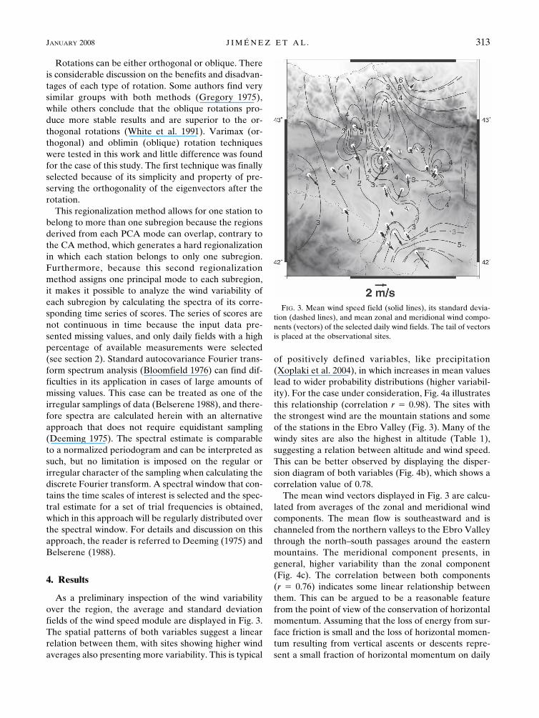
As a preliminary inspection of the wind variabilityover the region, the average and standard deviationfields of the wind speed module are displayed in Fig. 3.The spatial patterns of both variables suggest a linearrelation between them, with sites showing higher windaverages also presenting more variability. This is typical

of positively defined variables, like precipitation(Xoplaki et al. 2004), in which increases in mean valueslead to wider probability distributions (higher variabil-ity). For the case under consideration, Fig. 4a illustratesthis relationship (correlation r � 0.98). The sites withthe strongest wind are the mountain stations and someof the stations in the Ebro Valley (Fig. 3). Many of thewindy sites are also the highest in altitude (Table 1),suggesting a relation between altitude and wind speed.This can be better observed by displaying the disper-sion diagram of both variables (Fig. 4b), which shows acorrelation value of 0.78.

The mean wind vectors displayed in Fig. 3 are calcu-lated from averages of the zonal and meridional windcomponents. The mean flow is southeastward and ischanneled from the northern valleys to the Ebro Valleythrough the north–south passages around the easternmountains. The meridional component presents, ingeneral, higher variability than the zonal component(Fig. 4c). The correlation between both components(r � 0.76) indicates some linear relationship betweenthem. This can be argued to be a reasonable featurefrom the point of view of the conservation of horizontalmomentum. Assuming that the loss of energy from sur-face friction is small and the loss of horizontal momen-tum resulting from vertical ascents or descents repre-sent a small fraction of horizontal momentum on daily

FIG. 3. Mean wind speed field (solid lines), its standard devia-tion (dashed lines), and mean zonal and meridional wind compo-nents (vectors) of the selected daily wind fields. The tail of vectorsis placed at the observational sites.

JANUARY 2008 J I M É N E Z E T A L . 313

time scales, changes in the zonal (meridional) compo-nent resulting from the interaction of the wind withorographic obstacles will translate into the transfer ofmomentum to the meridional (zonal) component. Thus,changes in the zonal (meridional) wind component willoften be related to changes in the meridional (zonal)component, and ultimately sites showing higher vari-ability in one component should be expected to havea higher variability in the other component also. Thisrelation is an indication of common variability andsupports the joint treatment of both components inthe application of the vectorial PCA in the analysis ofthe wind variability instead of performing a separateanalysis on each variable component. As for the highermeridional than zonal variability, this is related (notshown) to the channeling of the flow between the largemountain systems in northern Spain (the CantabrianMountains and the Pyrenees; see Fig. 1), and at a moreregional scale within the CFN. Here, channeling is fa-vored along the northern valleys and the Ebro Valley,with a northwest–southeast orientation, and particu-larly around the eastern mountains systems, with anorth–south orientation. This behavior will be furtherillustrated with the results of the PCA analysis in thefollowing sections.

a. Regionalization using cluster analysis

The explained variance of the leading PCA modes ofthe wind field is shown in Fig. 5. There are breaks of the

slope at modes three and five, as well as a less clear oneat mode nine, which according to the scree test of Cat-tell (1966), are reasonable numbers of modes to retain.The retention of three of them might not be enough to

FIG. 5. The explained variance of the PCA modes. Notice thebreak in the vertical scale.

FIG. 4. (a) Mean daily wind speed vs its standard deviation for the selected days in the 35 sites, (b) altitude vs meanwind speed, and (c) standard deviation of the wind component vs standard deviation of the u wind component.

314 J O U R N A L O F A P P L I E D M E T E O R O L O G Y A N D C L I M A T O L O G Y VOLUME 47

adequately group the stations, because in such cases thesimilarity measure (2) would be calculated with thecontributions of only three terms, whereas nine modescould introduce noise into the classification because ofthe little variance explained by the higher-order modes.Therefore, five principal modes, which accumulate84.1% of the variance in the data, were retained. Theloading maps (eigenvectors) of these principal modesare displayed in Fig. 6. These maps represent flow di-rections and can be interpreted in their positive phaseas displayed either in Fig. 6 or in the opposite sign ofthe mode (corresponding to a negative sign in theirprincipal component). The first mode explains two-thirds of the variance (66.8%) and is well organized(Fig. 6a): the vectors are aligned along the valley axis,indicating that the dominant physical process is the to-pographical channeling. In the positive (negative)phase the main flow has a southeast–northwest (north-west–southeast) direction, while some mountain sitesseem to show a certain decoupling of the flow withrespect to the valley circulations, presenting a meridi-onal direction with a northward (southward) orienta-tion. The second principal mode explains 8.6% of thevariance and presents strong eastward (westward) flowsat the highest locations mainly, and weaker southwest–northeast (northeast–southwest) flows at the rest of thesites (Fig. 6b). Physically, this can be interpreted as theinfluence of the synoptic-scale flows, which is more in-tense at the higher sites. Therefore, this mode also re-veals a decoupling of the flow between mountain andvalley circulations, noted before. The third principalmode explains 3.4% of the variance. It shows activity inthe center of the region, with zonal directions in theflows but with opposite orientations at sites separatedby relatively small distances that could be associatedwith the recirculation or local behavior of the flow (Fig.6c). The fourth and fifth modes explain 2.9% and 2.4%of the variance, respectively, and show relations be-tween a few stations of each mode (Figs. 6d,e). The lowpercentage of variance explained by these last modescan be related to the limited size of their area of influ-ence relative to that of the three first modes. The im-proved knowledge of variability within this confinedarea could stem, in the future, from higher spatial sam-pling. This arrangement of explained variance is similarto that found by other authors in regions of comparablesize (Hardy and Walton 1978; Green et al. 1992; Lud-wig et al. 2004).

The first step of this CA regionalization is to grouptogether the stations with similar loads (Fig. 6) usingthe hierarchical CLA in order to decide the number ofsubregions to be formed. This was done by displayingthe sequence of distance measures at which the clusters

were merged in each step (Fig. 7). Because the CLAmerges the two most similar clusters at each step, alarge jump in the sequence means that two very differ-ent clusters have been merged, and indicates the con-venience of stopping the algorithm just before this hap-pens. Steps appear at six and nine clusters (Fig. 7), andtherefore they are a reasonable number of subregionsto form. The regionalization of nine subregions formsmany small groups with only one or two stations (Fig.8a); hence, a six-cluster regionalization was selected(Fig. 8b). After the CLA, the reordering of the stationsin the six selected subregions is performed by thenonhierarchical algorithm and provides the final windregionalization (Fig. 8c). This reordering only changesthe location of station number 32 (Fig. 1), which wasassigned to the first subregion by the CLA (Fig. 8b) andnow belongs to the third wind region (Fig. 8c). Thesimilar clustering of the stations obtained in the twosteps of the CA methodology grants robustness to theproposed regionalization. The Ebro Valley stationsform the first subregion (label 1 in Fig. 8c), the narrownorthern valleys are the second subregion (label 2 inFig. 8c), the high mountain stations are the third sub-region (label 3 in Fig. 8c), and the rest of the subregionsare small groups with a north-to-south orientation inthe center of the CFN (labels 4, 5, and 6 in Fig. 8c).Conceptually, this seems to suggest that there are threewell-defined regions, and a fourth one, the centralnorth-to-south area that groups the clusters with thelowest numbers of stations.

b. Regionalization using rotated principal modes

This method rotates the retained PCA modes to per-form the regionalization. Subregions are then formedretaining just the highest loads of each loading map.This is done by defining a critical threshold value, andonly those sites with loads exceeding it will belong tothe subregion. Hence, one subregion is created foreach rotated mode; the method allows for the forma-tion of overlapping subregions in opposition to the CAmethod, which generates a hard regionalization withoutpossible overlap. The retention of five modes, as wasdone with the regionalization using CA, results in astrong overlapping between the formed subregions andsuggests that five wind regions appear to be too many.Hence, only four principal modes were employed forthis regionalization method (81.7% of the variance). Aswas mentioned above, rotation tends to form simplestructures (Richman 1986) in which the variables are asclose as possible to the hyperplane of at least one prin-cipal mode. The degree of the simple structure can bevisualized displaying the loads of one principal mode

JANUARY 2008 J I M É N E Z E T A L . 315

FIG. 6. Loading maps of the first five principal modes are shown. The tails of the vectors are placed at theobservational sites. Explained variances for each mode are (a) 66.8%, (b) 8.6%, (c) 3.4%, (d) 2.9%, and (e) 2.4%.

316 J O U R N A L O F A P P L I E D M E T E O R O L O G Y A N D C L I M A T O L O G Y VOLUME 47

against those of another mode. Figure 9 shows an ex-ample of this for mode 1 versus 2 and 4, illustrating thatvalues overall tend to be closer to the axis in the rotatedcase. The effect of the varimax rotation is apparent inthe turning of the dispersion diagram of mode 1 versusthat of mode 4.

The loading maps of the four rotated principal modesin their positive phase are displayed in Fig. 10. Whencompared with the unrotated principal modes (Fig. 6),they show a clearer physical interpretation in some as-pects. The first and second rotated principal modes(Figs. 10a,b) present similar patterns to those of thefirst two modes (Figs. 6a,b). The first pattern presentsin its positive (negative) phase the southeast–northwest(northwest–southeast) channeling along the Ebro Val-ley, as in the unrotated case, and some minor differ-ences in the representation of its influence in the area

FIG. 7. The distance at which the last two clusters are mergedagainst the number of clusters formed is shown. The larger jumpat 6 and 9 suggests that these numbers of clusters should be re-tained.

FIG. 8. Wind regionalization obtained with the CLA ofthe five most important principal modes for the cases of (a)9 and (b) 6 subregions; (c) the wind regionalization ob-tained with the second step of the CA methodology, thenonhierarchical algorithm that reorders the 6 subregionsformed with the CLA as shown in (b).

JANUARY 2008 J I M É N E Z E T A L . 317

between the western and eastern mountains, where therotated mode indicates perhaps some clearer tilt to thenorth (south). The second mode (Fig. 10b) is also simi-lar to its unrotated analog (Fig. 6b), but with the vectorspresenting a clearer alignment along the eastward(westward) direction in the mountain stations and withweaker vectors (smaller loadings) in the valleys. Thethird rotated principal mode (Fig. 10c) presents meridi-onal orientation of the vectors, which show a southward(northward) sense in the eastern areas of the CFN, andzonal orientation with a westward (eastward) sense inwestern areas. In this case the pattern suggests a clearerbehavior of the wind flow bordering the western andeastern mountain obstacles from some north or north-east direction. A further analysis of the synoptic condi-tions related to these patterns would be convenient forunderstanding the regional behavior as a result of theinteraction of large-scale dynamics with topography.This is beyond the purposes of the regionalization atthis point, but some discussion along these lines will beintroduced in the last section. The fourth rotated prin-cipal mode (Fig. 10d) shows channeling flows along thenorthern valleys, and weak vectors in the Ebro Valleyand the mountain stations. In comparison with the lastunrotated vectors (Fig. 6) it distinctly highlights thechanneling of wind in the northern valleys.

After a visual inspection of the loading maps (Fig.10) a critical value for the vector modules can be de-fined in such a way that stations that exceed the thresh-old will define wind regions. As can be observed in Fig.10, the critical value must be chosen carefully in orderto avoid too much overlapping between either subre-gions or stations left ungrouped. Several critical valueswere tested, and finally the compromise was solved byadopting a critical module value of 0.175, which delim-its the most consistent subregions. The regionalizationobtained can be observed in Fig. 11a. The first subre-gion corresponds to the Ebro Valley (circles in Fig.11a), the second is mainly defined by the mountainstations (squares in Fig. 11a), the third groups stationslined up in a north–south direction from the innernorthern valleys up to the Bidasoa mountains and be-yond (diamonds in Fig. 11a), and the fourth is funda-mentally shaped by the northern valley sites (trianglesin Fig. 11a). This wind regionalization is very similar tothat obtained with the CA method (Fig. 6c). However,it clearly groups the sites labeled with diamonds (region3) as a whole region overlapping with the northern val-ley sites, instead of the various small groups providedby the CA. Moreover, this regionalization creates anextended group of mountain stations instead of the veryspecific individual high mountain sites identified by the

FIG. 9. Dispersion diagrams of principal mode 1 vs (a) mode 2 and (b) mode 4, and rotated mode 1 vs (c)rotated mode 2 and (d) rotated mode 4.

318 J O U R N A L O F A P P L I E D M E T E O R O L O G Y A N D C L I M A T O L O G Y VOLUME 47

CA regionalization method. However, this methodol-ogy has the drawback that there are two stations—10and 16 (Fig. 1)—that were not assigned to any group.When the critical value was reduced in an attempt toinclude them into a group, then the subregions over-lapped too much. Station 16 has the highest load mod-ule (0.168) for the Ebro Valley subregion, which agreeswith the assignment resulting from the CA regionaliza-tion; however, it also has a high load for the mountainregion (0.155). Station 10 has the highest load modulesfor the Ebro Valley subregion (0.171) and the northernvalleys subregion (0.169). These types of situationscould be ameliorated with further improvements in thetemporal length and spatial coverage of the dataset,which would allow for capturing better signals that arefaintly represented in the data.

c. Temporal variability

The second regionalization method, based on the ro-tation of the selected vectorial PCA modes, makes itpossible to examine the temporal wind variability ofeach subregion by analyzing the time series of the ro-tated scores. For illustrative purposes, the 20-day mov-ing-average filter outputs of the time series of scoresare displayed (Fig. 12). Each score presents differentbehavior showing the distinct wind variability in theformed subregions. However, the rotation of the prin-cipal modes involves the loss of the independence (zerocorrelation) property of the scores’ time series andtherefore, part of the variance accounted for by onemode could also be explained by other modes (Preisen-dorfer 1988). The correlation among the rotated scores’

FIG. 10. Loading maps of the four rotated principal modes with the varimax technique. The tails of the vectorsare placed at the observational sites. See Table 2 and Fig. 12 for complementary information.

JANUARY 2008 J I M É N E Z E T A L . 319

time series can be observed in Table 2. The correlationof 0.79 between score 1 (Ebro Valley) and 4 (northernvalleys) implies similar wind variability in these subre-gions. Indeed, the regionalization reached retainingthree principal modes (Fig. 11b) basically groups thestations from these two subregions. However, thefourth subregion in Fig. 11a is a well-defined clusterusing the CA regionalization methodology (Fig. 8c),and is fundamentally constituted by stations that sharea characteristic terrain feature, namely, location in thenorthern valleys. Thus, the decision was made to keepthis region as a different group on the basis of the re-sults with the CA method and the distinct topographi-cal character.

The time series of scores of each mode are comparedwith the mean wind components of each wind region inFig. 13. This allows for illustration of the meaning of thetime evolution of the principal components (scores) in

relation to changes in the zonal and meridional com-ponents in each region. The changes in the scores’ timeseries for each mode match in some regions with thoseof the zonal wind component, those of the meridionalcomponent, or with both. A common feature is that thefour subregions present a very similar evolution of theirmean meridional component, revealing that the vari-ability of this component is uniform over all of theCFN. However, the mean zonal component shows dif-ferent variability and is the actual factor that seems toplay a role in distinguishing subregions. The similarityof the time series of scores with the zonal or meridionalcomponents can be understood if the orientation ofvectors in the loading maps is taken into account (Fig.10). For instance, the Ebro Valley subregion shows asimilar evolution of the time series of scores and boththe series of the zonal (r � �0.93) and meridional (r �0.99) winds (Fig. 13a). This similar variability of both

FIG. 11. Wind regionalization obtained with the rotation of the (a) four and (b) three most important principalcomponent modes. The crosses represent the unclassified stations. The other symbols are defined in the text.

FIG. 12. The 20-day moving-average filter outputs of the time series of scores after varimaxrotation are shown.

320 J O U R N A L O F A P P L I E D M E T E O R O L O G Y A N D C L I M A T O L O G Y VOLUME 47

wind components seems to be associated with thenorthwest–southeast orientation of the Ebro Valleyand the channeling along it (Fig. 10a). This is also ap-parent in the fourth subregion (the northern valleys,see Fig. 13d), which also presents a northwest–south-east orientation of the valleys (Fig. 10d), with the me-ridional and zonal components similar to the score (r ��0.84 and r � 0.77, respectively). The mountain sub-region evolves in agreement (r � 0.94) with the meanzonal component of the subregion (Fig. 13b) in concor-dance with the zonal orientation of the vectors in itsloading map (Fig. 10b). Last, the scores in region 3 alsopresent similar changes (r � �0.66) to the zonal mean

wind component (Fig. 13c) resulting from the zonal ori-entation of the vectors with the highest loads at thestations that define the subregion in its loading map(Fig. 10c).

1) SPECTRAL ANALYSIS

Normalized spectra of the rotated scores provide acomplementary understanding of wind temporal vari-ability in each subregion (Fig. 14). The four subregionsshow wide spectral bands at low frequencies, althoughthey are not significant in comparison with a red-noiseautoregressive (AR1) process. It is worth noting thatthe time span of the series in Fig. 10 is only of about 3yr, and thus of limited extension for significantly resolv-ing the annual cycle. These low-frequency bands accu-mulate the largest portion of variance in all subregions.In addition, the various subregions accumulate varianceover specific intervals centered at periods that coincidewith harmonics of the annual cycle. However, few of

FIG. 13. The 20-day moving-average filter outputs of the timeseries of scores (solid lines) and the corresponding filtered u(dashed) and (dotted) standardized mean wind components ofthe corresponding wind region as defined by Fig. 11a: (a) EbroValley (region 1), (b) mountain stations (region 2), (c) north-to-south-oriented stations (region 3), and (d) northern valleys (re-gion 4).

TABLE 2. Correlation of the rotated scores.

Score 1 Score 2 Score 3 Score 4

Score 1 1.00 �0.25 0.06 0.79Score 2 �0.25 1.00 �0.29 �0.41Score 3 0.06 �0.29 1.00 0.09Score 4 0.79 �0.41 0.09 1.00

FIG. 14. Sample power spectra of the four principal componentscores after varimax rotation (solid lines), their first-order autore-gressive process spectra (dashed lines), and the 90% (dotted lines)and 95% (dashed–dotted lines) confidence limits. The spectrarepresent the wind variability in each of the following wind re-gions: (a) Ebro Valley (region 1), (b) mountain stations (region2), (c) north-to-south-oriented stations (region 3), and (d) north-ern valleys (region 4).

JANUARY 2008 J I M É N E Z E T A L . 321

these are of significance in comparison with an AR1.This is the case of the Ebro Valley (region 1) and thenorth-to-south-oriented sites (region 3), which displaysignificant portions of variance at frequencies rangingbetween 2 and 4 months. Spectra of the Ebro Valleyand the northern valleys subregion (Figs. 14a,d, respec-tively) turn out to be very similar, as should be expectedfrom their correlation (Table 2). However, the northernvalley sites do not seem to receive AR1-significant con-tributions at high frequencies.

For a more complete analysis of wind variability atlow frequencies, the standardized anomalies of dailywind time series from the original extended dataset canbe projected onto the eigenvector of each subregion inorder to reach longer time series than those in the ro-tated scores (769 days). Projections were performed forthe days with more than 50% of the measurementsavailable, and thus a total of 2169 days were used. Thisset spans over a period of more than 7 yr, from Febru-ary 1995 up to September 2002. For each subregion,both the original scores and the time series obtainedfrom projection are very similar in the overlappingparts, but the latter cover a longer time span, allowingfor increased spectral resolution at lower frequencies.Spectra for the projected time series are displayed inFig. 15. Overall, they show similar behavior as that ofthe score spectra (Fig. 14), with a gain in resolution anda suggestion of the presence of significant variability atyearly time scales relative to an AR1 process. As in thecase of Fig. 14, only the sites in the Ebro Valley (Fig.14a) and the north-to-south-oriented stations (Fig. 14c)show significant contributions at higher frequencies.Figures 14 and 15 suggest that the main difference be-tween the variability of the first (Ebro Valley) andfourth (northern valleys) subregions is the apparentlack of significant contributions to high-frequency vari-ability in the latter.

2) LARGE-SCALE INFLUENCE

Last, it can be argued that the regional variationsdescribed herein stem from the interaction of large-scale dynamics with regional topographic features andthat it is of interest to explain the temporal changes inthe behavior of each region on the basis of this inter-action. As stated before, a thorough analysis hereoncan be provided through calculation of a compositemap of the standardized mean sea level pressure select-ing the days on which the wind field at the surface levelis characteristic of the pattern of each mode or region.These characteristic days are selected as those thatpresent a maximum in the time series of scores (rotatedprincipal components). The maximum ensures that theprevailing flows are those defined by the loading map

of the subregion (Fig. 10) resulting from the dominanceof its score over the others. The composite maps of thesea level pressure for the five highest values of scores ateach subregion can be observed in Fig. 16. Variations inthe number of the selected days used to produce a com-posite do not essentially lead to different maps. TheEbro Valley subregion presents in its positive (nega-tive) phase a negative (positive) pressure anomaly innorthwestern Spain and a positive (negative) pressureanomaly in the west of Italy (Fig. 16a). This generates anortheastward (southwestward) geostrophic wind overthe CFN, which turns northward (southward) becauseof the ageostrophic balance. This flow is channeled up(down) the Ebro Valley (Fig. 10a) and is favored by thestrong pressure gradient along the valley axis that iscreated by the positive and negative anomaly maxima.Region 2 (mountains) shows a negative (positive) pres-sure anomaly in the north of France and a positive(negative) one in the west of the African coast (Fig.16b). This develops a southwestward (northwestward)geostrophic flow, which turns eastward (westward) as aconsequence of the ageostrophic balance. There is asmall pressure gradient along the Ebro Valley that con-tributes to the weak winds on the valley (Fig. 10b). The

FIG. 15. As in Fig. 14, but for the standardized projections of thedaily wind fields (with more than 50% of the data available) overthe eigenvectors.

322 J O U R N A L O F A P P L I E D M E T E O R O L O G Y A N D C L I M A T O L O G Y VOLUME 47

north-to-south-oriented stations (region 3) present adominant positive (negative) pressure anomaly in thenorth of the CFN (Fig. 16c). This anomaly generateswestward or southwestward (eastward or northeast-ward) ageostrophic winds over the CFN (Fig. 10c). Thenorthern valleys (region 4) present a strong negative(positive) pressure anomaly over northwestern Spain(Fig. 16d), which should generate similar winds over theCFN as the composite map of the Ebro Valley subre-gion (Fig. 16a). The structure of both composites is verysimilar, with larger negative anomalies over northwest-ern Spain and positive anomalies over the Mediterra-nean area, displaced to the south in Fig. 16d relative toFig. 16a. The similarity of both structures is not surpris-ing because the corresponding time series of scoreswere correlated (r � 0.79, see Table 2). The associatedregional maps (Figs. 10a,d) present differences in theloadings over the Ebro Valley, which are much smallerin region 4 (Fig. 10d). These regional differences cannotbe explained on the basis of the large-scale compositesin Fig. 16.

5. Conclusions

Daily wind variability over a complex terrain regionwas analyzed. Two different methodologies based onPCA were employed to make a regionalization intosubregions with similar time variability. The first ap-proach groups together stations with similar loads byCA producing a hard regionalization where the stationsbelong to only one subregion (Fig. 8c). The second ap-proach rotates the principal modes and forms subre-gions, allowing for some degree of overlapping (Fig.11a). Each methodology presents its own advantagesand drawbacks, and the use of both schemes allows fora good degree of robustness in conclusions; both pro-duce an equivalent array of groups, providing wind re-gions in accordance with the topographic features ofthe terrain. The main difference between the two meth-odologies is that the one based on CA generates anarea with a few small subregions that are joined by therotating methodology. The CA tends to form very spe-cific subregions, while the one based on the rotation

FIG. 16. Composite (averaged) maps of the standardized daily sea level pressure taken from the 40-yr EuropeanCentre for Medium-Range Weather Forecasts reanalysis data (Simmons and Gibson 2000) for the five maximumvalue scores of each subregion: (a) Ebro Valley (region 1), (b) mountain stations (region 2), (c) north-to-south-oriented stations (region 3), and (d) northern valleys (region 4).

JANUARY 2008 J I M É N E Z E T A L . 323

forms more generic groups. However, this regionaliza-tion that rotates the principal modes leaves two stationsunclassified. A higher density and coverage of stationsover the region would allow for a better identificationof smaller subgroups, and hence it would lead to a bet-ter characterization of the wind over the CFN.

The variability of the meridional wind is very similarin all of the subgroups, and it is the zonal wind compo-nent that mostly contributes to the characterization ofthe wind variability in each subregion. On the basis ofthis statement, it can be argued that a scalar PCA-basedapproach applied to the zonal component would lead tosimilar results. While this is essentially true, such anapproach would exclude the vectorial information, andthus the possibility of highlighting patterns of distinctwind direction over the CFN (e.g., channeling along thevalleys). The wind spectrum of each subregion was ana-lyzed, revealing the dominance of the annual cycle in allof them. Two subregions display significant variabilityat higher frequencies (2–4 months) in comparison withan AR1 process.

This wind regionalization will be used to validate me-soscale model simulations over the region. Because thesimulations represent spatially filtered conditions andthe observations could be affected by local effects thatfall beyond model resolution, their direct comparisonmay be somewhat problematic. With this regionaliza-tion, wind simulations/predictions can be evaluated ateach wind region, instead of at every measurement site,gaining significance in the validation procedure. Thiswill lead to a better knowledge of model performanceover the different wind regions and to potential im-provement of its accuracy.

With a broader perspective, the regionalization couldbe useful for analyzing the dispersion of pollutants overthe region, which would be different in the distinct sub-regions because of their different wind variability.Thus, the regionalization would be useful to evaluateimpacts of existing factories or future ones, helpingwith the industrial development of the region. The re-gionalization can also prove to be useful for potentiallyspreading the meteorological network, helping to lo-cate the new stations, or relocating those already exist-ing. It would be useful also for quality-control purposesbecause the stations in the same subregion shouldpresent similar wind variability. Moreover, it can beemployed to gain a better understanding of the rela-tionship between synoptic-scale motions and surfaceflows over the region, and of the physical processesassociated with wind circulations over the area.

Acknowledgments. We thank the Sección de Evalu-ación de Recursos Agrarios del Departamento de Ag-

ricultura, Ganadería y Alimentación of the NavarraGovernment for providing us with the wind datasetused in this study and the ECMWF for the free accessto the ERA-40 data. We also thank Drs. M. Montoyaand C. Raible for useful discussions, suggestions, andcomments during this work, as well as Prof. M. Cornidefor providing a first version of the code to calculate thespectral densities. The authors are indebted to the threereviewers for their comments, which helped to improvethe quality of the original manuscript considerably.This work was partially funded by Project CGL2005-06966-C07/CLI. JFGR was supported by a Ramón yCajal fellowship.

REFERENCES

Anderberg, M. R., 1973: Cluster Analysis for Applications. Aca-demic Press, 359 pp.

Bärring, L., 1988: Regionalization of daily rainfall in Kenya bymeans of common factor analysis. J. Climatol., 8, 371–389.

Belserene, E. P., 1988: Rhythms of a variable star. Sky and Tele-scope, Vol. 76, September, p. 288.

Bloomfield, P., 1976: Fourier Analysis of Time Series: An Intro-duction. Wiley, 258 pp.

Blumen, W., Ed., 1990: Atmospheric Processes over Complex Ter-rain. Meteor. Monogr., No. 45, Amer. Meteor. Soc., 323 pp.

Bonell, M., and G. Sumner, 1992: Autumn and winter daily pre-cipitation areas in Wales, 1982–1983 to 1986–1987. Int. J. Cli-matol., 12, 77–102.

Cattell, R. B., 1966: The scree test for the number of factors.Multivariate Behav. Res., 1, 245–276.

Cheng, E. D., 1998: Macroscopic extreme wind regionalization. J.Wind Eng. Ind. Aerodyn., 77–78, 13–21.

Comrie, A. C., and E. C. Glenn, 1998: Principal components-based regionalization of precipitation regimes across thesouthwest United States and northern Mexico, with an appli-cation to monsoon precipitation variability. Climate Res., 10,201–215.

Deeming, T. J., 1975: Fourier analysis with unequally-spaced data.Astrophys. Space Sci., 36, 137–158.

DeGaetano, A. T., 1997: A quality-control routine for hourlywind observations. J. Atmos. Oceanic Technol., 14, 308–317.

Dyer, T. G. J., 1975: The assignment of rainfall stations into ho-mogeneous groups: An application of principal componentanalysis. Quart. J. Roy. Meteor. Soc., 101, 1005–1013.

Fovell, R. G., and M.-Y. C. Fovell, 1993: Climate zones of theconterminous United States defined using cluster analysis. J.Climate, 6, 2103–2135.

Graybeal, D. Y., 2006: Relationships among daily mean and maxi-mum wind speeds, with application to data quality assurance.Int. J. Climatol., 26, 29–43.

Green, M., L. O. Myrup, and R. G. Flocchini, 1992: A method forclassification of wind field patterns and its application toSouthern California. Int. J. Climatol., 12, 111–135.

Gregory, S., 1975: On the delimitation of regional patterns ofrecent climatic fluctuations. Weather, 30, 276–288.

Hardy, D., and J. J. Walton, 1978: Principal components analysisof vector wind measurements. J. Appl. Meteor., 17, 1153–1162.

324 J O U R N A L O F A P P L I E D M E T E O R O L O G Y A N D C L I M A T O L O G Y VOLUME 47

Johnson, S. C., 1967: Hierarchical clustering schemes. Psy-chometrika, 32, 241–254.

Kaihatu, J. M., R. A. Handler, G. O. Marmorino, and L. K. Shay,1998: Empirical orthogonal function analysis of ocean surfacecurrents using complex and real-vector methods. J. Atmos.Oceanic Technol., 15, 927–941.

Kaufmann, P., and R. O. Weber, 1996: Classification of mesoscalewind fields in the MISTRAL field experiment. J. Appl. Me-teor., 35, 1963–1979.

——, and ——, 1998: Directional correlation coefficient for chan-neled flow and application to wind data over complex terrain.J. Atmos. Oceanic Technol., 15, 89–97.

——, and C. D. Whiteman, 1999: Cluster-analysis classification ofwintertime wind patterns in the Grand Canyon region. J.Appl. Meteor., 38, 1131–1147.

Klink, K., and C. J. Willmott, 1989: Principal components of thesurface wind field in the United States: A comparison ofanalyses based upon wind velocity, direction, and speed. Int.J. Climatol., 9, 293–308.

Ludwig, F. L., J. Horel, and C. D. Whiteman, 2004: Using EOFanalysis to identify important surface wind patterns in moun-tain valleys. J. Appl. Meteor., 43, 969–983.

Mass, C. F., and Y.-H. Kuo, 1998: Regional real-time numericalweather prediction: Current status and future potential. Bull.Amer. Meteor. Soc., 79, 253–263.

McGowan, H. A., and A. P. Sturman, 1996: Interacting multi-scale wind systems within an alpine basin, Lake Tekapo, NewZealand. Meteor. Atmos. Phys., 58, 165–177.

Meek, D. W., and J. L. Hatfield, 1994: Data quality checking forsingle station meteorological databases. Agric. For. Meteor.,69, 85–109.

Milligan, G. W., 1980: An examination of the effect of six types oferror perturbation on fifteen clustering algorithms. Psy-chometrika, 45, 325–342.

Preisendorfer, R. W., 1988: Principal Component Analysis in Me-teorology and Oceanography. Elsevier, 425 pp.

Richman, M. B., 1986: Rotation of principal components. Int. J.Climatol., 6, 293–335.

Rife, D. L., C. A. Davis, Y. Liu, and T. T. Warner, 2004: Predict-ability of low-level winds by mesoscale meteorological mod-els. Mon. Wea. Rev., 132, 2553–2569.

Romero, R., C. Ramis, J. A. Guijarro, and G. Sumner, 1999a:Daily rainfall affinity areas in Mediterranean Spain. Int. J.Climatol., 19, 557–578.

——, G. Sumner, C. Ramis, and A. Genovés, 1999b: A classifica-tion of the atmospheric circulation patterns producing signifi-cant daily rainfall in the Spanish Mediterranean area. Int. J.Climatol., 19, 765–785.

Simmons, A. J., and J. K. Gibson, 2000: The ERA-40 Project Plan.ECMWF ERA-40 Project Rep. Series 1, Reading, UnitedKingdom, 63 pp.

Sotillo, M. G., C. Ramis, R. Romero, S. Alonso, and V. Homar,2003: Role of orography in the spatial distribution of precipi-tation over the Spanish Mediterranean zone. Climate Res., 23,247–261.

Steinacker, R., and Coauthors, 2006: A mesoscale data analysisand downscaling method over complex terrain. Mon. Wea.Rev., 134, 2758–2771.

Stewart, J. Q., C. D. Whiteman, W. J. Steenburgh, and X. Bian,2002: A climatological study of thermally driven wind sys-tems of the U.S. Intermountain West. Bull. Amer. Meteor.Soc., 83, 699–708.

Stooksbury, D. E., and P. J. Michaels, 1991: Cluster analysis ofsoutheastern U.S. climate stations. Theor. Appl. Climatol., 44,143–150.

von Storch, H., 1995: Inconsistencies at the interface of climateimpact studies and global climate research. Meteor. Z., 4,72–80.

——, and F. W. Zwiers, 1999: Statistical Analysis in Climate Re-search. Cambridge University Press, 484 pp.

Weber, R. O., and P. Kaufmann, 1995: Automated classificationscheme for wind fields. J. Appl. Meteor., 34, 1133–1141.

White, D., M. Richman, and B. Yarnal, 1991: Climate regional-ization and rotation of principal components. Int. J. Climatol.,11, 1–25.

Whiteman, C. D., 2000: Mountain Meteorology: Fundamentalsand Applications. Oxford University Press, 355 pp.

——, and J. C. Doran, 1993: The relationship between overlyingsynoptic-scale flows and winds within a valley. J. Appl. Me-teor., 32, 1669–1682.

Wilks, D. S., 1995: Statistical Methods in the Atmospheric Sciences:An Introduction. Academic Press, 467 pp.

Xoplaki, E., J. F. González-Rouco, J. Luterbacher, and H. Wan-ner, 2004: Wet season Mediterranean precipitation variabil-ity: Influence of large-scale dynamics and trends. ClimateDyn., 23, 63–78.

JANUARY 2008 J I M É N E Z E T A L . 325