Economic Regionalization and Numerical Methods - RCIN
246
Economic Regionalization and Numerical Methods Geographia Polonica 15
-
Upload
khangminh22 -
Category
Documents
-
view
0 -
download
0
Transcript of Economic Regionalization and Numerical Methods - RCIN

Economic
Regionalization
and Numerical
Methods
Geographia Polonica 15

http://rcin.org.pl

Geographia Polonica 15
Economic Regionalization and Numerical Methods
http://rcin.org.pl

e o g r a p h i
P o l o n i c a
15
http://rcin.org.pl

INSTITUTE O F GEOGRAPHY POLISH ACADEMY OF SCIENCES G E O G R A P H I A P O L O N I C A 15
Economic Regionalization and
Numerical Methods Final Report oî the Commission
on Methods of Economic Regionalization oî the International Geographical Union
Edited by
BRIAN J. L. BERRY with ANDRZEI WRÓBEL
Państwowe Wydawnictwo Naukowe Warszawa 1968
http://rcin.org.pl
Editorial Board
S T A N I S Ł A W LESZCZYCKI (Editor-in-Chief), JERZY KONDRACKI, JERZY KOSTROWICKI, JANUSZ PASZYŃSKI,
ANDRZEJ W E R W I C K I (Secretary), Z U Z A N N A SIEMEK (Deputy Secretary)
Adress of Editorial Board KRAKOWSKIE PRZEDMIEŚCIE 30, WARSZAWA 64
POLAND
Printed in Poland
PAŃSTWOWE WYDAWNICTWO NAUKOWE (PWN — POLISH SCIENTIFIC PUBLISHERS)
WARSZAWA 1968
Drukarnia Uniwersytetu im. A. Mickiewicza w Poznaniu
http://rcin.org.pl

CONTENS
Preface 7
I
Kazimierz Dziewoński — Economic Regionalization. A Report of progress 9 List of publications issued by or under the auspices of the I.G.U. Commission
on Methods of Economic Regionalization 23 Review of Articles on the activities of the Commission on Methods of Economic
Regionalization 23
II
Introductory Note 25 Brian J. L. Berry —- Numerical Regionalization of Political-economic space 27 Boris B. Rodoman (Translated by T. Shabad) — Mathematical aspects of the
Formalization of Regional Geographic Characteristics 37 Barclay G. Jones and William W. Goldsmith — A Factor Analysis Approach
to Sub-regional Definition in Chenango, Delaware, and Otsego counties 59 Teresa Czyż — The Application of Multifactor Analysis in Economic Regio-
nalization 115 John D. Nystuen and Michael F. Dacey — A Graph Theory Interpretation of
Nodal Regions 135 Benjamin H. Stevens and Carolyn A. Brackett — Regionalization of Pennsyl-
vania Counties for Development Planning 153 Stanisław Lewiński — Taxonomic Methods in Regional Studies . . . 189 D. Michael Ray — Urban Growth and the Concept of Functional Region 199
http://rcin.org.pl

http://rcin.org.pl

PREFACE
This volume is the last of the series containing the research and work undertaken by the Commission on Methods of Economic Regionalization of the International Geographical Union in the years 1960—1968. It is divided in two parts. The first one contains the final report on the activities of the Commission, together with the lists of publications of the Commission and of the reviews of its activities published in various periodicals. The second part presents a collection of papers on the nu-merical methods as applied in the economic regionalization, the nature of which is explained in the introductory note by B. J. L. Berry.
In prefacing this last official publication of the Commission it is my pleasant duty to express the words of gratitude to all the institutions and persons who enabled the Commission to function and to do some research studies. In particular I thank:
— the International Geographical Union for establishing the Com-mission and for the organizational and financial help;
— the Polish Academy of Sciences and the Institute of Geography of that Academy for financing the Secretariate of the Commission, for organizing one of its meetings (in Jablonna, in 1963) as well as covering the costs of its publications;
— the Resources for the Future, Inc. and the University of Chicago for support of research;
— the Czechoslovak Academy of Sciences and its Institute of Geo-graphy for organizing one of the meetings of the Commission (in Brno, in 1965) and for publication of its proceedings;
— the University of Strasbourg, France and Centre National de la Recherche Scientifique for their help in organizing one of the meetings of the Commission and of an International Symposium on "Regionali-zation and Development" (in Strasbourg, in 1967);
— the University of Utrecht for being the host to our first meeting (in 1961);
— all other institutions such as the Institutes of Geography of the Academies of Sciences of Bulgaria, Czechoslovakia, Hungary, Poland, Rumania and the U.S.S.R, Centre National de la Recherche Scientifique
http://rcin.org.pl

8 P R E V A C E
(France), National Science Foundation (USA) and others which by co-vering travel costs of the individual members of the Commission helped in realization of its programme.
Finally I would like to thank on behalf of the Commission and per-sonally, Prof. Andrzej Wróbel and Miss Halina Gudowska for unremit-ient carrying on of secretarial and editorial duties for the Commission during eight years of its existence.
Kazimierz Dziewoński Chairman
http://rcin.org.pl

G E O G R A P H I A P O L O N I C A 15
ECONOMIC REGIONALIZATION. A REPORT OF PROGRESS
KAZIMIERZ DZIEWONSKI
When in 1950 at the XIX International Geographical Congress held in Stockholm the Commission on Methods of Economic Regionalization had been formed its aims were defined as follows: f t . . . to analyse and compare the ends and means of geographical research on the problems of economic regionalization. undertaken in various countries, both from the point of view of its value for the development of scientific theory and of its practical application" 1.
To realize these tasks three surveys were undertaken covering main research problems in the field, i.e. (a) basic concepts and theories, (b) methods of research, and (c) practical applications 2. On their basis three important aspects of economic regionalization were agreed on at the First General Meeting in Utrecht (1961) as significant for further discussion, namely: (a) the most rational division of a country for some practical purposes, mainly for administration and planning; (b) existing regional structure of economy and economic regions as developing within this structure; (c) regional method of analysis and related geo-graphical research techniques. The programme for further work establis-hed at the Second General Meeting in 1963 (Jablonna) included among others: preparation of an international bibliography of books and papers on economic regionalization; studies on the historical development of economic regionalization — its concepts, methods and application as a part of the development of geographical sciences; studies concerned with methods of economic regionalization in particular with quantitative statistical and cartographical ones; analysis of the present regional eco-nomic structure together with the study of the integrated economic regions; studies of interrelations between scientific research in the field of economic regionalization and the practical needs of human community;
1 The IGU Newsletter, XII, 1, 1961, p. 47. 2 Report of the First General Meeting of the Commission in Utrecht The IGU
Newsletter, XII, 1962, p. 27.
http://rcin.org.pl

10 K A Z I M I E R Z D Z I E W O Ń S K I
comparative studies of the administrative structure of the countries in the whole world and finally typological studies of economic regions on comparative basis 3.
All these studies were carried on and discussed during the following Third, Fourth, and Fifth General Meetings of the Commission held in London (1964), in Brno (1965) and in Strasbourg (1967). With the work of the Commission approaching its closing (the mandate ends in 1968 at the X X I International Geographical Congress to be held in Delhi), a general review of all studies both fully accomplished and undertaken but so far not completed seems to be necessary. They will be grouped under five headings: (A) the development of basic concepts in the field of economic regionalization; (B) methods used in studies of economic regionalization; (C) the general theory and typology of economic regions; (D) the role of regional structures and economic regions in the economic development, and (E) practical applications of economic regionalization together with a comparative study of administrative and planning di-visions.
THE DEVELOPMENT OF BASIC CONCEPTS IN THE FIELD OF ECONOMIC REGIONALIZATION
In the last eight years since the establishment of the Commission some progress in the systematic historical study of the developments of basic concepts has been achieved. The critical bibliographies for the United States 4, for the Soviet Union 5 and for France 6 were published. Similar bibliographies for Great Britain and Commonwealth countries (by F. E. I. Hamilton), as well as for German speaking countries (by S. Schneider) and for the European socialist countries are practically finished and should be finished in time for the Delhi Congress. We possess also some interesting historical papers on the developments ir. the United States (by. G. W. Hoffman) 7, in Germany (by G. W. Hoffman
Report of the Second General Meeting of the Commission in Jabłonna, Po-land. The IGU Newsletter, XV, 1/2, 1964, p. 49—50.
4 Brian J. L. Berry and Thomas D. Hankins, A Bibliographical Guide to the Economic Regions of the United States, Chicago, 1963, pp. XVIII, 101.
5 W. W. Pokshishevskii, Bibliografiya Sovietskoi Literatury po Ekonomiches-komu Rayonirovaniyu. Obzor Opublikovannoi Bibliografii, Ekonomicheskoe Rayo-nirovanie SSSR, Moskva, 1965, pp. 131—145.
3 P. Claval and E. Juillard, Région et régionalisation dans la géographie française et dans d'autres sciences sociales. Bibliographie analytique. Cahiers de l'Institut d'Etudes Politiques de L'Universite de Strasbourg, III, Paris, 1967, p. 99
' George W. Hoffman, Development of Regional Geography in the Unitec States, Economic Regionalization, Proceedings of the Fourth General Meeting oj
http://rcin.org.pl
E C O N O M I C R E G I O N A L I Z A T I O N 11
and by R. Klopper) 8, in France (by E. Juillard)9 and in England (by F. E. J. Hamilton)10. We should also note a larger study by A. Wrobel on the concept of an economic region in the theory of geography n . Howe-ver, the intended full and systematic study involving complete mastery of the geographical literature in the last two centuries turned out — at least for the present — to be inachievable.
Nevertheless on the basis of the existing histories of geographical thought and obtained new studies it is possible to distinguish three basic independent although correlated concepts of "economic region" widely used by geographers of all countries and nationalities. These are:
1. Regions (areal units)— basis and tool for research (including sta-tistical areas);
2. Regions—tools for action (organizational e.g. administrative or planning regions);
3. Regions—goal and results of research in the way of regional analysis. This third kind may be split into two subgroups: (a) regions— —goal and results of research, and (b) regions—object of research (objective regions)12.
The first of these concepts is historically the latest. It emerged from the critical review of the so-called "regional method". Its theory was never fully explored and developed. There are some very pertinent remarks on its subject in a handbook on use of statistics in geography, published in 1961 by three American authors13.
As in its case it would be comparatively easy to drop completely the use of the term "region" and to replace it by the term "areal unit", it will not be discussed here in greater detail. It is sufficient to notice
the Commission on Methods of Economic Regionalization, September 7—12, 1966, Brno, Czechoslovakia, Prague, 1967, pp. 37—63.
8 George W. Hoffman, op. cit., pp. 59—63; R. Klopper, Die Entwicklung des re-gional Konzept in der deutschen Geographie. Paper presented at the Fifth General Meeting of the Commission on Methods of Economic Regionalization in Stras-bourg, 1967.
u E. Juillard, Histoire de la notion de région dans la géographie française, Région et regionalization ... (see footnote 6), pp. 9—20.
10 F. E. J. Hamilton, The Establishment of Economic Region in Great Britain. Paper presented at the Fifth General Meeting of the Commission on Methods of Economic Regionalization, Strasbourg, 1967.
11 A. Wróbel, Pojęcie regionu ekonomicznego a teoria geografii (The Concept of Economic Region and the Theory of Geography), Prace Geograficzne, 48, War-szawa, 1965, p. 87 (Summary in English).
12 See papers presented by H. Bobek and K. Dziewoński at the Brno Meeting, Economic Regionalization . . . (see footnote 7), pp. 17—30.
13 O. D. Duncan, R. P. Currort and B. Duncan. Statistical Geography. Problems in Analysing Areal Data, Chicago, 1961, pp. XIV, 191.
http://rcin.org.pl
12 K A Z I M I E R Z D Z I E W O Ń S K I
that in practice it is often identified with the grid of some type of ad-ministrative division (region—tool for action) and its use in the study of the regions of the third kind (i.e. regions—goal and result of research) involves either basic independence from the divisions of actual regional structures or complete identification with such structures. In the first case the best solution is in the use of abstract, purely geometrical grids (however they have to be rather of small scale or dense in relation to the studied structures). In the second case a good antecedent knowledge of these structures is necessary at the beginning of the research. Further pertinent observations on these problems may be found in the paper prepared by T. Hagerstrand for the Brno Meeting 14.
The second concept dominates in most of the present practical appli-cations of geographical research, specially in the economic and physical planning. To eliminate in this case the use of the term "region" seems impossible. Such regions-tools for action—are obviously correlated with regions-goal and result of research, but their complete identification is unobtainable. The first ones have to represent the division of the whole space into definite and complete number of areal units, in most cases of the same or similar size (whatever measure of size, such as an area or a number of population or some other one shall be assumed). In case of hierarchical division simple and full aggregation of smaller into the larger units is expected. The second ones are both by implication of their definition and in reality of different size, rarely completely filling up the whole space and often overlapping, but only partly, one another. Nevertheless they have a deep influecne, one set on another the organizational regional division never being able to separate com-pletely from the objective regional structures or even aiming directly for some kind of identification with such structures and the same struc-tures adjusting themselves more or less over time to organizational di-visions.
The third concept of a region is the most debatable one especially in its full form of the so-called "objective regions". For some, affirmation of their existence becomes a point of honour, for others it is a point of deep scepticism (it is very difficult to identify them) or even of complete agnosticism (it is impossible to find them). However it is the oldest and probably the most persistent idea or even ideal in the devel--opment of the geographical thought and theory.
Professor Bobek in his Brno paper 15 described more precisely various positions. Clearly the settlement of the dispute is at present out of
u T. Hagerstrand, Geographic Information for Computer Work in Sweden, Economic Regionalization ... (see footnote 7), pp. 107—122.
15 Op. cit. (see footnotes 12 and 7).
http://rcin.org.pl
E C O N O M I C R E G I O N A L I Z A T I O N 13
cur reach but at least it is possible to indicate some way out of difficulties. In my opinion, this lies in the study of the correlation of the different regions and regional patterns as established through really scientific studies and research. All these are included by Professor Bobek under a heading of "regions—goal and result of research". All form together what after A. Wróbel1 6 may be called "regional structure" of an area, a space. When they to intergrate — at least partially — in a siggnificant way, then we may speak of "region —object of research (objective region)". Further study of such regions, their taxonomy and typology should lead us to the general regional theory.
The introduction of the supplementary term in the form of "eco -nomic region" does not change these general remarks although evidently it narrows the whole field of discussion. Here, however, an additional point of differences does arise. What implies the qualification "economic" which we put beside the basic term and concept "region". Some, mainly in the United States and in Western Europe, by use of the term "eco -nomic" imply that they limit the field of their analysis to the economic activities and phenomena only; others, especially the geographers influ-enced by the Marx theory and concepts, imply only that the economic factor or aspect in the human affairs is the most significant, in fact, the decisive one. To avoid misunderstandings it seems preferable in such a case to speak of "socio-economic regions".
Two meanings of the term "regionalization"—as "a division of space" or as "some kind of procedure for establishing specific division of space" are generally accepted and, so far, do not lead to any serious misunder-standings. The meaning actually used is always easy to discern from the whole context of a given reasoning.
Various additional terms are introduced often in the discussion of problems of economic regionalization. They are usually connected with some specific theory of economic regions and their concrete meanings are defined within the statement of theory. Only one pair of them, i.e. "homogeneous" and "nodal regions" led to a very heated controversy— rather in result of their actual use of the terms of the differences as to their meaning. We shall discuss this problem later on when dealing with methods of economic regionalization. A short warning should, however, be given here as to the meaning and use of the terms "hie-rarchy" and "hierarchical regions". The Oxford Dictionary gives a gene-ral meaning of the term—"any graded organization". It is too easily assumed that the hierarchical system of regions has to be simple, com-
1B A. Wróbel, WojewodzUvo warszawskie. Studium ekonomicznej struktury regionalnej (The Warsaw Voivodship. A Study of Regional Economic Structure). Prace Geograficzne, 24, Warszawa, 1960, p. 140, (Summary in English).
http://rcin.org.pl

14 K A Z I M I E R Z D Z I E W O Ń S K I
plete, and uniform. In reality they are very often either complex, i.e. they form together a loosely knit combination of simpler systems or partial, i.e. the regions in some part of the analysed space form a hier-archical system, or multivarious, i.e. the grading of regions varies in contents, form and space throughout the whole system.
METHODS USED IN STUDIES OF ECONOMIC REGIONALIZATION
From the beginning, the studies and discussions within the Com-mission were concentrated on the methods used in establishing regional structures and economic regions—goal and result of research. At the Jabłonna Meeting in 1963, Chancy D. Harris presented a comprehensive report on methods used in Argentina, Austria, Belgium, Bulgaria, Ca-nada, Czechoslovakia, Denmark, Finland, France, Germany, Great Bri-tain, Hungary, India, Japan, Yugoslavia, Mexico, The Netherlands, Nor-way, Southern Africa, Sweden and the United States 17. His study inclu-ded also a bibliography composed of 291 publications. In presenting the whole collected material he used the traditional for the United States division into uniform (sometimes called also homogeneous) and organi-zational (also called nodal or, improperly, functional) regions. Such a division was strongly questioned by a Russian geographer P. M. Alam-piev 18. In the heated discussion on the subject there is a large number of misunderstandings. The division is of formal character, it serves for classification of methods and in reality does not necessarily imply any theoretical or ideological bias. However even from the formal point of view it is not fully satisfactory as the division is not logically exclu-sive and it is even possible with specific treatment of data to define the organizational regions as the uniform ones. A better, more definite and still formal way of classifying methods of analysis seems to be that into scalar and vector regions, i.e. regions defined on the basis of scalar and vector values. Such a definition explains easily why it is possible to treat, to a certain extent, the organizational—now the vector regions as the uniform ones, i.e. the scalar regions 19.
Thi;s statement marks the transition from the general review of traditional methods to the study of possible applications of mathematical analysis in the economic regionalization. The reports prepared by B. J. L.
17 Methods of Economic Regionalization. Proceedings of the Second General Meeting of the Commission on Methods of Economic Regionalization, September 9—13, 1963 at Jabłonna, Poland. Geographia Polonica, 4, 1964, pp. 59—86.
18 Op. cit., pp. 143—145. 19 K. Dziewoński, Théorie de la région économique. Mélanges Tulippe, Liège,
1967, pp. 818—830. Also: Teoria regionu ekonomicznego, Przegląd Geograficzny, 39, 1967, pp. 33—50 (Summaries in English and Russian).
http://rcin.org.pl

E C O N O M I C R E G I O N A L I Z A T I O N 15
Berry for the Brno 20 and the Strasbourg 21 Meetings provide an excellent basis for the appreciation and discussion of the new methodological approach. This started with the application for regionalization of the multifactor analysis. Originally such an analysis was limited to the regions characterized by similarities in scalar values. Later on Berry and others introduced vector values (in form of dyadic data) for characteri-zation of regions by similarities in interrelations and finally evolved techniques for correlating and evolving regions characterized both by scalar and vector values. In this way the formal duality of uniform and organizational regions was overcome and the doors are open for the for-mulation of integrated methodology of research of regional structures and economic regions. This takes form of a general field theory22 , i.e. of a spatial system that comprises places, the attributes of these places and the interactions among them. The theory is at present a rather com-plex one, although mathematically easily comprehensible. In my personal opinion, some important simplifications are possible and indeed, in the near future, shall be introduced. But even now a great step forward has been achieved.
Obviously other approaches in the use of mathematical methods for economic regionalization are possible although none was so clearly de-fined and developed as the multi-factor analysis. One of them seems to be rather promising—the use of graph theory for establishing the area of a region and for measuring its internal cohesion 23.
An interesting effort define the logical bases for use of mathematical and cartographical methods in studies of regionalization was made by a Soviet geographer B. B. Rodoman24 . This study is of special value because of its systematic development of concepts permitting the full application of mathematical methods.
20 Economic Regionalization ... (see footnote 7), pp. 77—106. 21 See below, p. 27. 22 Brian J. L. Berry et al., Essays on Commodity Flows and the Spatial Struc-
ture of the Indian Economy, University of Chicago, Dept. of Geography, Research Paper 111, Chicago, 1966, pp. viii, 354.
23 J. Czarnecki, Metoda grafów w zastosowaniu do analizy codziennych do-jazdów pracowniczych, Biulletin de I'Academie Polonaise des Sciences. Also: S. Bartosiewiczowa and J. Czarnecka, Przyczynek do problemu codziennych do-jazdów pracowniczych (A Contribution to the Problem of Everyday Commuting to Work), Przegląd Geograficzny, 38, 1966, pp. 725—745.
24 B. B. Rodoman, Logicheskie i kartograficheskie formy rayonirovaniya i za-dachi ikh izucheniya. Izviestiya AN SSSR, Seriya geograficheskaya, 4, 1965, pp. 113—126. Reprinted as: The Methods of Individual and Typological Regionalization and Their Mapping, Soviet Geography, 11, 1965; B. B. Rodoman, Matematicheskie aspekty formalizatsii porayonnykh geograficheskikh kharakteristik, Vestnik Mo-
http://rcin.org.pl

16 K A Z I M I E R Z D Z I E W O Ń S K I
GENERAL THEORY AND TYPOLOGY OF ECONOMIC REGIONS
Any greater progress in the development of a theory depends more on individual efforts than on collective studies and discussions. However last years brought in some interesting achievements and the existence of the Commission was an important factor., a catalyst in their elabo-ration.
As already mentioned Brian J. L. Berry came inductively by way of the multi-factor analysis to the formulation of a general field theory. This is an important step as, in my opinion, any general theory of eco-nomic regionalization has to be theory of economic or better socio-eco-nomic time-space; an economic region being by definition a subspace in such a space. The problems of economic regions within the socio-econo-mic space were developed deductively by K. Dziewoński in several papers 25. As such a space is not clearly homogeneous—the field theory is an obvious and convenient but not the only solution. An outstanding theoretician in this field is W. Warntz 26 who starts from the concept of population potential and by extending it to the income potential comes very near to the full measurement of the socio-economic space. One factor still missing in this basic structure of an economic space is the value of fixed assets as changing throughout the socio-economic time--space. These three factors: the number of population, the size of na-tional income and the value of fixed assets, each measured i relation to a areal units, taken together characterize fully—at least in general aspects—the socio-economic field and may serve as the frame of refe-rence to the structural and typological studies of economic regions.
The above-mentioned theories of the socio-economic space possess a rather formal i.e. abstract and mathematical character. They have to be supplemented or rather integrated into the historical and geographical theory of regional development based on the scientific achievements of political economy and sociology.
Consistent interest in the theory of economic regions as important factors in the national economy is shown by Soviet geographers as well as by geographers of other socialist countries 27. Here we clearly stand
skovskogo Universiteta, Geografia, 2, 1967, pp. 28—44 (English translation in this volume).
25 Among others: On Economic Regionalization, Geographia Polonica, 1, 1964, pp. 171—185; Problems of Integration of Cartographical and Statistical Analysis, Regional Science Association, Papers, XV, 1965, pp. 119—129; Théories de la région économique, Melanges Tulippe, Liège 1967, pp. 818—830.
26 w . Warntz, Macrogeography and Income Fronts, Regional Science Research Institute, Monograph Series 3, Philadelphia, 1965, p. 117.
27 The latest among very many publications are: A. M. Kolotievskiy, Voprosy teorii i metodiki ekonomicheskogo rayonirovaniya (v sviazi s obshchey teoryey
http://rcin.org.pl
E C O N O M I C R E G I O N A L I Z A T I O N 17
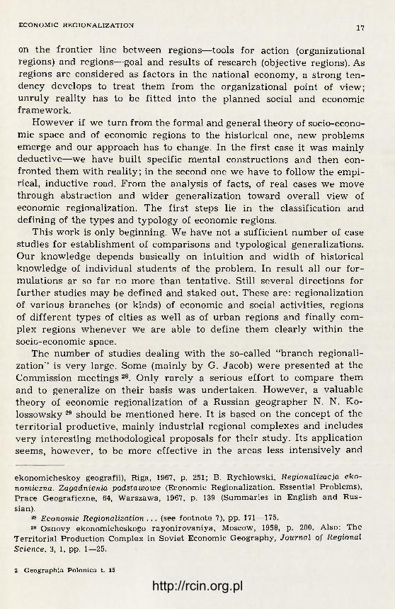
on the frontier line between regions—tools for action (organizational regions) and regions—goal and results of research (objective regions). As regions are considered as factors in the national economy, a strong ten-dency develops to treat them from the organizational point of view; unruly reality has to be fitted into the planned social and economic framework.
However if we turn from the formal and general theory of socio-econo-mic space and of economic regions to the historical one, new problems emerge and our approach has to change. In the first case it was mainly deductive—we have built specific mental constructions and then con-fronted them with reality; in the second one we have to follow the empi-rical, inductive road. From the analysis of facts, of real cases we move through abstraction and wider generalization toward overall view of economic regionalization. The first steps lie in the classification and defining of the types and typology of economic regions.
This work is only beginning. We have not a sufficient number of case studies for establishment of comparisons and typological generalizations. Our knowledge depends basically on intuition and width of historical knowledge of individual students of the problem. In result all our for-mulations ar so far no more than tentative. Still several directions for further studies may be defined and staked out. These are: regionalization of various branches (or kinds) of economic and social activities, regions of different types of cities as well as of urban regions and finally com-plex regions whenever we are able to define them clearly within the socio-economic space.
The number of studies dealing with the so-called "branch regionali-zation'' is very large. Some (mainly by G. Jacob) were presented at the Commission meetings 28. Only rarely a serious effort to compare them and to generalize on their basis was undertaken. However, a valuable theory of economic regionalization of a Russian geographer N. N. Ko-lossowsky 29 should be mentioned here. It is based on the concept of the territorial productive, mainly industrial regional complexes and includes very interesting methodological proposals for their study. Its application seems, however, to be more effective in the areas less intensively and
ekonomicheskoy geografii), Riga, 1967, p. 251; B. Rychłowski, Regionalizacja eko-nomiczna. Zagadnienia podstawowe (Economic Regionalization. Essential Problems), Prace Geograficzne, 64, Warszawa, 1967, p. 139 (Summaries in English and Rus-sian).
28 Economic Regionalization . . . (see footnote 7), pp. 171—175. 29 Osnovy ekonomicheskogo rayonirovaniya, Moscow, 1958, p. 200. Also: The
Territorial Production Complex in Soviet Economic Geography, Journal of Regional Science, 3, 1, pp. 1—25.
2 Geographia Polonica t. 15
http://rcin.org.pl

18 K A Z I M I E R Z D Z I E W O Ń S K I
only recently developed where the whole structure of production is com-paratively simple and the physical distances make the development of more complex and criss-crossing relations or even dependencies rather difficult.
The problem of regional areas connected with cities and in particular with larger cities is from various points of view (case studies, theoretical generalizations, fully fledged theories) very welle developed indeed. I will not review it here in closer detail as there are some extensive studies of the subject30 and my own publications are among them 31. All that should be said here is that all materials and theories need careful investigation— in the light of latest changes and developments in the cha-racter and structure of urban regions—out of which perhaps a more satisfactory and better integrated theory of urban network and urban areas will finally emerge.
Obviously studies of complex regions are basic for the theory of economic regionalization. There are not enough of them in spite of the fact that regional monographs belonging to the venerable tradition of the work undertaken villingly by geoghraphers are very numerous. The reason is that only rarely a conscious effort was made to define such a rtegion and to explain its structure and relations with the external larger world in terms of some theory of economic regionalization. Studies based on multi-factor analysis, as those already mentioned by B. J. L. Berry and his followers 32, were recently developed and were based on subtle and sophisticated concepts of fundamental spatial patterns (struc-ture matrix replacing the attribute matrix), types of spatial behaviour (behaviour matrix replacing the interaction matrix) and their interde-pendences again in another matrix. However these studies are so far few and limited at the best to a single country (nation or state) and therefore cannot be used as yet for the comparative analysis. The theory of the socio-economic time-space and of the economic region as a subspace, as tentatively formulated by K. Dziewoński33 shows that we should not expect economic regions either to be defined by the same elements (attri-butes and relations) or to represent an universal and discrete division of
30 Among others: Ph. M. Hauser and L. F. Schnore, Echton, The Study of Ur-banization, New York, 1965, pp. IX, 554; J. Beaujeu-Garnier and G. Chabot, Traité de géographie urbaine, Paris, 1963, p. 493.
31 Specially: Baza ekonomiczna i struktura funkcjonalna miast. Studium roz-woju pojęć, metod i ich zastosowań (Urban Economic Base and Functional Structure of Cities. A Study of the Development of Concepts, Methods and Applications), Prace Geograficzne, 63, Warszawa, 1967, p. 135 (Summaries in English and Russian).
32 See footnote 22. See footnote 25.
http://rcin.org.pl

E C O N O M I C R E G I O N A L I Z A T I O N 19
space or to form together a full and consistent hierarchy. Nevertheless, to construct a typology of economic regions we have to use some kind of classification and this has to be connected with a specific procedure. Before we are able to formulate such a classification and procedure on the basis of empirical studies (using perhaps the multi-factor analysis) a working hypothesis is needed. In my opinion this should take form of a socio-economic table in which all the basic, significant factors in the development of human community (in this case the regional commu-nity) will be taken systematically into account. For the construction of such a table the Marxian concepts, on the one hand, and those of Le Play and Geddes, on the other, should and may be easily used.
Some interesting typological proposals were recently presented by the French geographer. Kayser.34 In analysing the growth of economic regions in the under-developed countries, he distinguished five kinds of economic spaces and regional formations from the point of view of their genesis. They are: (a) indifferent space, i.e. without distinct regional economic divisions; (b) regions of speculative enterprises; (c) regions of intervention, e.g. regions developing around specific investiment pro-ject, undertaken for the community; (d) urban or metropolitan basins; and (e) organized regions, i.e. developing out of administrative and poli-tical divisions. This kind of typology clearly shows both the possibilities and difficulties of such a classification.
Although the typology of smaller economic regions is not yet really developed the situation improves when we move to the larger ones, in particular to the independent states. Without doubt this is due, at least partly, to the fact that a state is at present the most fully established and crystallized form of an economic region. It represents a closed social economic system with well defined unequivocal points of entrance and exit as well as clearly demarcated frontiers. In the strong majority of cases the closed within the state-region part of the social and economic activities is significantly stronger than the open part. There exist gene-rally accepted groupings of contemporary states which moreover are con-venient for our purposes. There are, on the one hand, the division on the basis of the stage of economic development (well developed, deve-loped and developing states) and, on the other, the division on the basis of the socio-economic system (capitalist and socialist countries as well as those of mixed economies—the so-called "Third World"). But as R. Gajda 35 in his paper and the following discussion in Brno have shown, there exists another differentiation of great importance based on diffe-
34 B. Kayser, Les divisions de l'espace geographique dans les pays sousdevelop-pes, Annales de Geographie, 76, 1966, pp. 686—697.
35 Economic Regionalization . . . (see footnote 7), pp. 145—159.
2*
http://rcin.org.pl

20 K A Z I M I E R Z D Z I E W O Ń S K I
rences in the density of population and the intensity of land utilization. In result these two elements of differentiation may serve as the working hypothesis for classification of regional structure of various countries throughout the world.
On a similar basis N. Ginsburg with the aid of B. J. L. Berry 36 and later S. Leszczycki37 worked out the typology of states and proposals for the division of the world into economic macroregions.
The typology of regional structures developed in such a way (either in the scale of the whole world or on a comparative basis for various countries) leads up to the new problem raised in the work to the Com-mission only recently, namely to the role played by the economic regio-nalization in the processes of economic development.
THE ROLE OF REGIONAL STRUCTURES AND ECONOMIC REGIONS IN THE ECONOMIC DEVELOPMENT
Although this problem has come to the surface rather late in the activities of the Commission its importance was realized immediately. In fact the programming of the whole Strasbourg Meeting was organized to explore its possibilities. Beside its value for practical applications of the concepts of economic regionalization it involves a dynamic approach as opposed to the static analysis, traditional in studies of economic re-gions in well and intensively developed countries. The role of regional structures in economic development has to be studied as they fluctuate, dying out and evolving, opposing and advancing the general growth of economy. Economic regions are seen as real elements (changing subspa-ces) of the social and economic time-space and not any more as per-manent features of the economic landscape.
At the Strasbourg Meeting it was possible to capitalize the very rich experience and knowledge of economic regionalization in developing coubtries, gained by French geographers in the research undertaken in Africa, Latin America and Southern Asia 38. In the light of their studies as well as of the studies of geographers of other countries it is possible to state that whenever the economic growth takes place suddenly or at a very quick rate the traditional small regions of local character are disrupted and transformed and new much larger regions quickly emerge. However, both these phenomena lead up to a rather disbalanced struc-
36 An Atlas of Economic Development, University of Chicago, Dept. of Geo-graphy, Research Papers 69, Chicago, 1.961, p. 119.
37 S. Leszczycki, Map of the Economic Regions of the World, Economic Re-gionalization . . . (see footnote 7).
33 See reports by O. Dolphus, J. Gallais, B. Kayser, J. Servais, J. Tricart, and others. Also already mentioned (footnote 34) article of B. Kayser.
http://rcin.org.pl

ECONOMIC R E G I O N A L I Z A T I O N 21
tare where intermediary forms are either underdeveloped or even com-pletely missing. Naturally, this introduces very strong tendencies towards concentration and even centralization. It is paradoxical that this same phenomenon is characteristic both for underdeveloped and strongly de-veloped economies whenever the economic growth has taken or takes palce in new, sparsely populated countries. On the other hand, in old countries of old standing and with large and dense population, even if pre-sently they are underdeveloped, the regional structure is more balanced and able to withstand the impact of an increased growth.
Naturally these are only the preliminary observations. Further stu-dies and research are still necessary, specially as the question of the role whether positive or negative of various regional and different types of socio-economic regions in the processes of economic growth has still to be fully clarified.
Another important problem for further study and clarification is the role of natural resources in the development both of the whole economy and of the regional structure and economic regions of a country. This problem, somewhat obscured by the ancient but now rejected theories of geographic determinism, is of specific interest for geographical scien-ces. Its solution involves the development of specific concepts bridging the distance between the geographical environment and its resources as they exist in reality, as they are known to the given human community and as they may be utilized by the same community. The growth in the knowledge and in the technique, conditioned as they are by human needs, are the decisive dynamic factors in the economic development while the resources themselves represent olny the potential, the static wealth out of which human communities supply their neds. But the concepts themselves form only the initial step toward the solution of the question. The comparative studies of specific communities are neces-sary. Thier results will serve in turn for the further development of once more partial theory of economic regionalization. The work starting presently under the direction of A. Mints should be of great help for this purpose. This should be based on achievements in this direction of the Soviet geographers and economists.
PRACTICAL APPLICATIONS OF ECONOMIC REGIONALIZATION
The efforts of the Commission to systematize the applications of eco-nomic regionalization in practical life have, generally speaking, failed in spite of a number of papers prepared for the Commission 39. This was
39 For instance papers by M. Blazek, K. Edwards, G. Jacob, E. Juillard, Ch. Ma-
http://rcin.org.pl
22 K A Z I M I E R Z D Z I E W O Ń S K I
due among others to the wealth of such applications. Moreover the large number of those applications is contained in numerous, published and unpublished, official and semi-official reports, often confidential or of restricted circulations.
However one kind of application, namely the use of studies for estab-lishing new or revising existing administrative divisions has led the Commission to a more detailed review of such applications and from there to the comparative study of these divisions. With the use of more modern methods of analysis some very interesting results were obtained by M. Blazek and E. Juillard40. Among others it was found that the disparities are not as large as usually assumed and that they may be easily classified in relation to their historical genesis, density of present population as well as the intensity of economic development.
* *
*
In the eight years of its existence the Commission, in spite of all the vicissitudes, was able to obtain the collaboration of a large number of geographers tu undertake some research and to discuss basic pro-blems included in its terms of reference. In some cases its efforts have failed, in other they remain to be continued or completed by others, but in several—a serious progress was obtained and the results will be valid for a longer period of time. If the systematization of basic concepts and terms, agreed within the Commission, will generally be accepted and followed, if the methods, especially mathematical methods as developed in the studies edited for the Commission will be generally but correctly used, if the bibliographies and reports serve geographers of all countries in their work—then all the efforts of the Commission have been worth-while and its work may even be considered well done. Still some ot the studies have to be continued. Let us hope that there will be one from among new commissions of the International Geographical Union created at the Delhi Congress which will willingly carry this work on.
rinov, S. Schneider, O. Tulippe and A. Wróbel, presented at the First General Meeting in Utrecht; these by C. Herbot, C. Ileśić, K. Ivanicka, E. Juillard, H. Ken-ning and J. Wilmet, at the Second General Meeting in Jabłonna, Poland; these by A. Bassols Batalia, R. Gajda and J. G. Saushkin, at the Third General Meeting in London; and these by M. Stfida and O. Tulippe, at the Fourth General Meeting in Brno.
40 For the preliminary reports see: Economic Regionalization... (see footnote 7) pp. 219—247. The final report is to be published by the Institute of Geography of the Czechoslovak Academy of Sciences in form of a separate volume.
http://rcin.org.pl
E C O N O M I C R E G I O N A L I Z A T I O N 23
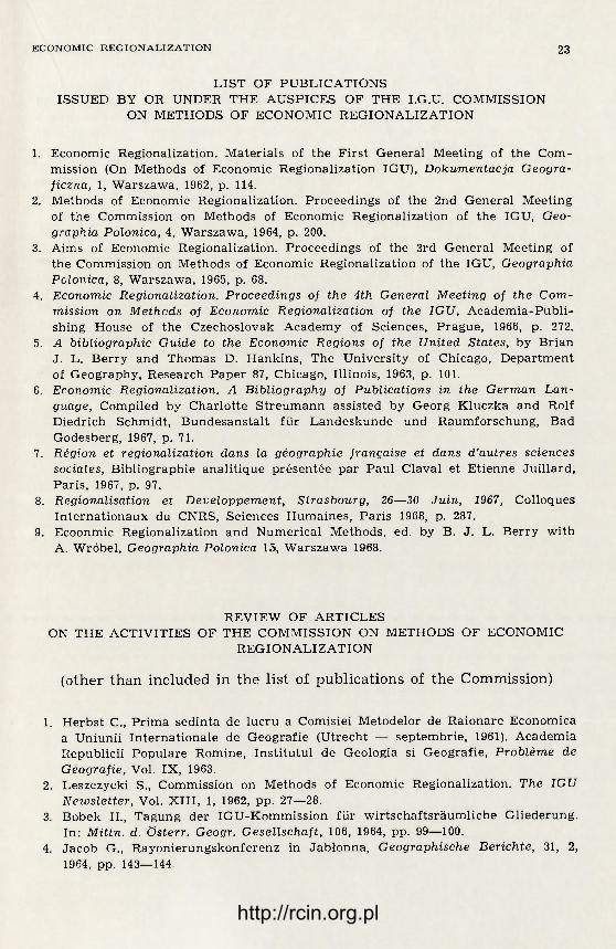
LIST OF PUBLICATIONS ISSUED BY OR UNDER THE AUSPICES OF THE I.G.U. COMMISSION
ON METHODS OF ECONOMIC REGION ALIZATION
1. Economic Regionalization. Materials of the First General Meeting of the Com-mission (On Methods of Economic Regionalization IGU), Dokumentacja Geogra-ficzna, 1, Warszawa, 1962, p. 114.
2. Methods of Economic Regionalization. Proceedings of the 2nd General Meeting of the Commission on Methods of Economic Regionalization of the IGU, Geo-graphia Polonica, 4, Warszawa, 1964, p. 200.
3. Aims of Economic Regionalization. Proceedings of the 3rd General Meeting of the Commission on Methods of Economic Regionalization of the IGU, Geographia Polonica, 8, Warszawa, 1965, p. 68.
4. Economic Regionalization. Proceedings of the 4th General Meeting of the Com-mission on Methods of Economic Regionalization of the IGU, Academia-Publi-shing House of the Czechoslovak Academy of Sciences, Prague, 1966, p. 272.
5. A bibliographic Guide to the Economic Regions of the United States, by Brian J. L. Berry and Thomas D. Hankins, The University of Chicago, Department of Geography, Research Paper 87, Chicago, Illinois, 1963, p. 101.
6. Economic Regionalization. A Bibliography of Publications in the German Lan-guage, Compiled by Charlotte Streumann assisted by Georg Kluczka and Rolf Diedrich Schmidt, Bundesanstalt für Landeskunde und Raumforschung, Bad Godesberg, 1967, p. 71.
7. Région et regionalization dans la géographie française et dans d'autres sciences sociales, Bibliographie analitique présentée par Paul Claval et Etienne Juillard, Paris, 1967, p. 97.
8. Régionalisation et Développement, Strasbourg, 26—30 Juin, 1967, Colloques Internationaux du CNRS, Sciences Humaines, Paris 1968, p. 287.
9. Ecoonmic Regionalization and Numerical Methods, ed. by B. J. L. Berry with A. Wróbel, Geographia Polonica 15, Warszawa 1968.
REVIEW OF ARTICLES ON THE ACTIVITIES OF THE COMMISSION ON METHODS OF ECONOMIC
REGIONALIZATION
(other than included in the list of publications of the Commission)
1. Herbst C., Prima sedinta de lucru a Comisiei Metodelor de Raionare Economica a Uniunii Internationale de Geografie (Utrecht — septembrie, 1961). Academia Republicii Populäre Romine, Institutul de Geologia si Geografie, Problème de Geografie, Vol. IX, 1963.
2. Leszczycki S., Commission on Methods of Economic Regionalization. The IGU Newsletter, Vol. XIII, 1, 1962, pp. 27—28.
3. Bobek H., Tagung der IGU-Kommission für wirtschaftsräumliche Gliederung. In: Mittn. d. Osterr. Geogr. Gesellschaft, 106, 1964, pp. 99—100.
4. Jacob G., Rayonierungskonferenz in Jabłonna, Geographische Berichte, 31, 2, 1964, pp. 143—144.
http://rcin.org.pl

24 K A Z I M I E R Z D Z I E W O Ń S K I
5. Jacob G., Zweite Hauptversammlung der IGU Kommission für Methoden der ökonomischen Rayonierung, Petermanns Geogr. Mitt., 108, 1—2, 1964, pp. 97—98.
6. Schneider S., Tagung der IGU-Kommission "On Methods of Economic Regio-nalization" in Jabłonna (Polen vom 9—13 September, 1963). In: Ber. z. dt. Landeskunde, 1, 1964, pp. 79—81.
7. Wróbel A., II Plenarne Zebranie Komisji Metod Regionalizacji Ekonomicznej MUG w Jabłonnie (Second General Meeting of the Commission on Methods of Economic Regionalization of the IGU in Jabłonna), Przegląd Geograficzny, 36, 1964, pp. 197—199.
8. Leszczycki S., Commission on Methods of Economic Regionalization, The IGU Newsletter, XV, 1/2, 1964, pp. 48—51.
9. Blazek M., Ctverte plenarni zasedani komise pro metody ekonomickeho rajono-vani v Brne, Sbornik cs. Spol. Zemepisne, 71, 1966, pp. 60—62.
10. Marianek V., Ctvrte zasedani komise pro metody ekonomicke rajonizace Mezi-narodni Geograficke Unie, Zpravy Geografickeho Ustavu CSAV Opava, 2, 1966, pp. 1—17.
11. Mints A. A., Chetvertoye plenarnoye zasedanie Komissii po metodam eko-nomicheskogo rayonirovaniya Mezhdunarodnogo Geograficheskogo Sojuza, Iz-vestiya Akademii Nauk SSSR — Seriya Geogr., 6, Moskva, 1965, pp. 124—126.
http://rcin.org.pl

INTRODUCTORY NOTE
These papers represent the culmination of a program of research by the Commission on Methods of Economic Regionalization of the Inter-national Geographical Union. The particular focus here is the exploration of existing and the development of new mathematical methods of eco-nomic regionalization. The important original contributions have been, in sequence:
(a) Development of a factor-analytic and grouping methodology for homogeneous regionalization.
(b) Extension of this grouping philosophy to the case of functional regions by use of the concept of a dyad.
(c) Utilizing the dyadic formulation to construct a general field the-ory of spatial behavior.
One report of the work is in my book Essays on Commodity Floats and the Spatial Structure of the Indian Economy. The purpose of the present volume is to provide both a review and an introduction to what we now prefer to call Numerical Regionalization.
A variety of individuals have been of inestimable assistance in this work. Particular thanks are due Peter Neely and Rudolph Rummel.
Brian J. L. Berry, April 14, 1967
http://rcin.org.pl

http://rcin.org.pl

G E O G R A P H I A P O L O N I C A 15
NUMERICAL REGIONALIZATION OF POLITICAL-ECONOMIC SPACE
BRIAN J. L . BERRY
Any space consists of a set of objects, characteristics of these objects, and interrelations among them. In the political-economic space that is the focus of this paper the objects of study are areas. The space com-prises an interface between economic characteristcs of areas (and, more basically, of the people and activities within them) and economic inter-relations among them on the one hand, and political characteristics and interrelations on the other, particularly as the latter are expressed through regional planning mechanisms.
Two perspectives may be taken in the definition and description of the political-economic space from the economic side:
(a) formal description of the properties of areas, often leading to their classification into relatively homogeneous types and subtypes;
(b) functional definition of the interrelations among the objects, again often concluding in the identification of groups or subgroups of highly connected areas.
A third perspective is added from the political viewpoint: (c) teleological analysis of the sources and areas of decision or power,
the grouping of areas that makes most sense for administrative coherence or for decision-making in planning, and of final planning objectives for the political-economic space.
Differences between the first two and the third perspectives are sources of tension, for frequently there is little congruence between the separate realities of economic and political space. Too often, the political--economic interface is characterized by discordance and lack of sym-metry. Occasionally, homogeneous economic areas may suggest problems needing solution, or a functional economic area may be the relevant impact-region within which both primary and secondary benefits of public investment programs are captured. Even less frequently, a funct-ional unit (such as a river basin) may be the proper systems-planning region (as in water management of the basin). More frequently, however, fragmented political jurisdictions cut across the realities of economic
http://rcin.org.pl
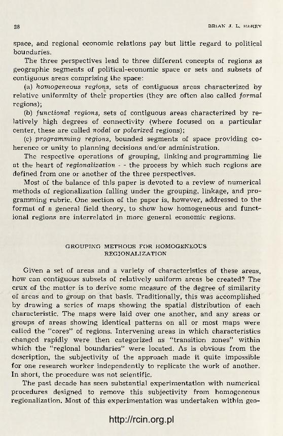
28 B R I A N J. L. B E R R Y
space, and regional economic relations pay but little regard to political boundaries.
The three perspectives lead to three different concepts of regions as geographic segments of political-economic space or sets and subsets of contiguous areas comprising the space:
(a) homogeneous regions, sets of contiguous areas characterized by relative uniformity of their properties (they are often also called formal regions);
(b) junctional regions, sets of contiguous areas characterized by re-latively high degrees of connectivity (where focused on a particular center, these are called nodal or polarized regions);
(c) programming regions, bounded segments of space providing co-herence or unity to planning decisions and/or administration.
The respective operations of grouping, linking and programming lie at the heart of regionalization — the process by which such regions are defined from one or another of the three perspectives.
Most of the balance of this paper is devoted to a review of numerical methods of regionalization falling under the grouping, linkage, and pro-gramming rubric. One section of the paper is, however, addressed to the format of a general field theory, to show how homogeneous and funct-ional regions are interrelated in more general economic regions.
GROUPING METHODS FOR HOMOGENEOUS REGIONALIZATION
Given a set of areas and a variety of characteristics of these areas, how can contiguous subsets of relatively uniform areas be created? The crux of the matter is to derive some measure of the degree of similarity of areas and to group on that basis. Traditionally, this was accomplished by drawing a series of maps showing the spatial distribution of each characteristic. The maps were laid over one another, and any areas or groups of areas showing identical patterns on all or most maps were called the "cores" of regions. Intervening areas in which characteristics changed rapidly were then categorized as "transition zones" within which the "regional boundaries" were located. As is obvious from the description, the subjectivity of the approach made it quite impossible for one research worker independently to replicate the work of another. In short, the procedure was not scientific.
The past decade has seen substantial experimentation with numerical procedures designed to remove this subjectivity from homogeneous regionalization. Most of this experimentation was undertaken within geo-
http://rcin.org.pl

N U M E R I C A L R E G I O N A L I Z A T I O N 3.1
graphy independently of parallel classificatory work in other fields. The satisfying result has been, however, that separate work in a variety of disciplines has converged on acceptable procedures of numerical taxonomy that aid the grouping process, although by no means all of the detailed considerations of regionalization are solved.
There are many good examples of multivariate homogeneous regio-nalization in the literature today (see the concluding Notes on Examples of this essay, plus the papers by Barclay G. Jones and William W. Gold-smith and by Benjamin H. Stevens and Carolyn A. Brackett that follow in this book — respectively A Factor Analysis Approach to Sub-Regional Definition in Chenango, Delaware and Otsego Counties and Regional-ization of Pennsylvania Counties for Development Planning). Because there are good examples to which the reader may turn, a brief outline of the complete series of steps in the preferred procedure of numerical taxonomy should suffice to indicate its nature:
(a) Assemble a table listing areas in the rows (as many rows as areas) and characteristics in the columns (as many columns as characteristics). Here, the decisions to be made are: how many units of observation and how many characteristics are relevant to the study. The table is called a data matrix.
(b) Find, where necessary, a normalizing transformation for each of the characteristics, and apply it to create a normalized data matrix.
(c) Calculate the correlation among each characteristic and every ether, and also arrange in a matrix.
(d) Perform a factor analysis of the correlation matrix. Here, a de-cision must be made about the number of meaningful factors to be used subsequently in the grouping analysis, what clusters of characterisitics these factors represent, and what the substantive meaning of each factor is. In part, these decisions are interpretive and external to the mathe-matics, although the mathematical procedures do provide relevant guides in the form of factor loadings, communalities, and eigenvalues.
(e) Create a table of factor scores — index numbers providing a da-tum for each area on each factor retained after step (d). Usually these factor scores will be orthonormal.
(f) Imagine the scatter diagram of the areas located in the space of the factors with the factor scores determining locations on the refe-rence axes, and compute the Euclidean distance between each area and everjy other. The distance measures are indexes of the relative similarity or homogeneity of the areas.
(g) Prepare a linkage tree successively grouping the most homoge-neous pair or subset of contiguous areas into larger sets or subsets. Se-veral alternative algorithms are available which produce slightly diffe-
http://rcin.org.pl

30 B R I A N J. L. B E R R Y
rent results, and a choice must be made among them according to their relative merits for the problem in hand.
(h) Decide on how many "cuts" across the complete linkage tree are significant. Each cut defines a given number of regions or subregions. The succession of cuts describes a regional hierarchy with each earlier cut identifying the subregions of each succeeding cut. There are as many levels of branching of the tree as there are cuts.
External decisions must be made by the regional analyst in steps (a), (d), (g) and (h). The nature and effects of these decisions are clear, however, and the mathematics ensure that any research worker making the same decisions will be able to replicate identical results. Since each of the decisions needed is in some sense a substantive one, it is doubtful that further mathematicization of the process is called for — in essence, a numerical solution now exists that goes as far as the mathematics probably should.
LINKAGE METHODS FOR FUNCTIONAL REGIONALIZATION
A variety of methods of functional regionalization also have been tried. Again, the method preferred traditionally was one of f low map comparison and generally was restricted to nodal regions focused on a limited set of centers. Later work extended this approach by use of gravity models. In the early mathematicization, the theory of graphs was applied to interactions of a particular kind between a prescribed set of nodes (for example, in the follownig paper by John D. Nystuen and Michael F. Dacey on A Graph Theory Interpretation of Nodal Re-gions that looks at telephone traffic between cities in the State of Washington — see also the handicraft methods in the Stevens-Brackett paper).
Some moments of reflection show that a simple extension of the concept of an observation makes it possible to apply the identical form of numerical regionalization outlined in the previous section of this paper to both the homogeneous and functional cases, however. The trick is simply to replace areas as observations by dyads — pairs of obser-vations between which flows move — and then to use as characteristics the types of flows that are of interest. For example, in my recently published book entitled Essays on Commodity Flows and the Spatial Structure of the Indian Economy basic data were available on 63 kinds of commodities moving among 36 areas, so that a 1260 X 63 matrix could be prepared and analyzed (there are 362 — 36 possible pairs of areas between which commodities could flow — the dyads). With only this
http://rcin.org.pl
N U M E R I C A L R E G I O N A L I Z A T I O N 3.1
change, application of process (a) through (h) yields a functional regio-nalization.
In both cases, the contiguity constraint in step (g) yields a regionali-zation. Elimination of the constraint often results in a typology — a classi-fication of areas into groups more uniform than contiguous regions, but often non-adjacent. In both, each characteristic and factor is accorded an equal weight, which is the best choice in the absence of alternative information on the relative importance of either initial variables or in-termediate factors. Particularly in the linkage case, however, additional processing of the data may be suggested, for example using relative rather than absolute flows, or flows with size and/or distance-decay factors taken out by means of gravity models. Each of these considera-tions represents an extra external decision, however.
HOMOGENEOUS AND FUNCTIONAL REGIONS RELATED BY A GENERAL FIELD THEORY
The dyadic form of numerical regionalization provides a means of synthesizing homogeneous and functional regions and, more generally, of modeling the complete space. There have been many attempts of this kind in the past (and two are reported in the Stevens-Brackett paper, and in D. Michael Ray's Urban Growth and the Concept of Functional Region, which also follows). Step (f) in the homogeneuos case provides a distance or similarity measure for each pair of areas, or could be tooled to provide such a pair-wise distance measure for areas on each factor separately, or on any selected combination of factors. These similarities are dyadic, and parallel, in the homogeneous case, factor scores created for dyads in step (e) of the functional case, where each factor score is a datum concerning the strength of some type of connectivity (distances in step (f) of the functional case actually compare the connectivity of pairs of dyads).
Two tables are therefore available. Each has rows occupied by the same dyads. The homogeneous case has as many columns as there are types of distance measure, and the functional case has a column for each type of connectivity. The general field theory says that the two sets of numbers are mutually interdependent. A change in either the degree of similarity or of connectivity of any pair of areas has reciprocal effects on the other. Patterns in one mirror patterns in the other.
Canonical analysis is used to mathematicize the field theory. In brief, it creates congruent pairs of factors from the two tables such that these factors are maximally correlated. Successive sets of factors reproduce,
http://rcin.org.pl

32 B R I A N J. L. B E R R Y
them, the various dimensions of interdependence of areas, thier cha-racteristics and interactios — in brief, these factors span and model the main dimensions of the complete space that is of interest. Each pair of vectors has dyadic measures of a maximally-correlated set of simi-larity and connectivity characteristics, and by extension of a maximally--correlated homogeneous and functional regionalization.
Very often, because similarities are symmetric (the similarity of 1 and 2 is the same as the converse) but connectivities are not, the relative location of pairs of points in the space needs to be taken into account to establish their proper relationships. Thus, a positive sign to a distance--similarity will indicate that, for da j is greater than i, and a negative sign will say that i exceeds j. This ordination often removes a serious form of confounding of relationships that is possible in the canonical formulation.
Without a contiguity constraint, grouping procedures applied to the results of canonical analyses identify general fields within the space of concern. By analogy, insistence upon contiguity ensures the creation of congruent homogeneuos-functional regions, or general regions.
HOMOGENEOUS, FUNCTIONAL AND GENERAL REGIONS IN REGIONAL PLANNING
A homogeneous regionalization would, it would seem, serve (by means of factor analysis) to identify the variety of existing types of planning problems that are present within the areas and characteristics, and by the regionalization, their concentration i particular kinds of problem areas. Such areas have often been the objects of regional planning pro-grams. The now-defunct Area Redevelopment Administration in the United States, for example, focused its attention and its investment programs in areas defined by unemployment and/or income criteria, to cite one example. A similar philosophy is evidenced by the eligibility criteria used to determine areas within cities that are to be subjected to urban renewal treatment.
On the other hand, a functional regionalization serves to identify linkages between areas, and thus, for example, the interdependencies to be exploited by a growth-center regional planning strategy such as advocated by a Perroux or a Boudeville. The more advanced growth--center philosophies recognize the spatial organization of towns and cities within any advanced economy into a central-place hierarchy, because market-oriented manufacturing activities and the whole array of func-tions needed in the tertiary sector have to be performed as efficiently
http://rcin.org.pl
N U M E R I C A L R E G I O N A L I Z A T I O N 3.1
as possible. Different orders of growth centers are then recognized, and to each order there is an appropriate array of investment alterna-tives determined by the size of market controlled by centers at each level of the hierarchy. Linkages relevant to the functional organization are goods, person, and money flows between central-places and surround-ing market areas, with the particular categories of linkages or flows shifting from one level of the hierarchy to another. The immediate impact-area of an investment located in a central-place is that place's market area, which usually also coincides with its market.
General regions produced by a field theory formulation will link various levels of homogeneous regionalization with the several levels of the urban hierarchy, frequently in an alternating sequence. Thus, for any order of central-place and market area there will be an immediate homogeneous sub-regionalization into a more developed center and a lagging periphery, to cite one frequent example. A growth center philosophy seeks to exploit this relationship.
One particular level of such a general regionalization has often been cited as being of especial importance in regional planning, the functional economic area. This is the level at which the market area (approximately the highest order of retail market, and the principal wholesale market area, too) and labor market of the central-place coincide, so the resulting region embrace both place of work of the residents and place of residence of the workers. An approximate accounting equality thus exists between income earned and income spent. Ragional acnunts for functional econo-mic areas are natural units into which national product accounts can be disaggregated. The growth center strategy seems particularly appro-priate when applied to such units, for a public investment in the central--place has its primary and secondary effects confined within the unit, and the lagging periphery is the logical area of spillover from the center.
PLANNING REGIONS
Planning regions have at one time or another been equated with pro-blem areas — a homogeneous concept — with functional units such as river basins or watersheds, and with growth-point centered development regions — a more general field concept. Often, too, instead of special planning districts being created, the planning region has been equated with some existing governmental jurisdiction, such as a county or a city, or a state. It is obvious that either engenders tensions, in the former case more of a political kind between the new jurisdiction and existing layers
3 G e o g r a p h i a Polonica t. 15 http://rcin.org.pl

34 B R I A N J. L. B E R R Y
of gouvernment, and in the latter of an economic kind, as the existing government finds that the array of economic forces it needs to mani-pulate as beyond its jurisdictional control.
The immediate reaction is that regionalization of the political-econo-mic space should result in units that are larger than the socio-economic entities that are to be affected, so that relevant planning variables are kept endogenous rather than remaining as unexpected and often capri-cious and confounding exogenous circumstances.
Eut what regionalization makes this possible? The answer is not to be found initially in the existing socio-economic or political realities, but in the goals of the planning process. First, one must determine what the socio-economic space might look like when the planning objectives are achieved. Here, a variety of techniques are useful, but perhaps the most satisfactory and elegant are programming models (see for example the Stevens-Brackett paper). Programming techniques can describe the state of the system — and its homogeneous and functional regionali-zations — at some end-point of goal-achievement. The question is then, what set of programming regions will enable the goals to be achieved. One role is that they should be large enough so that policy makers have all relevant variables available endogenously. The question may then be raised as to whether existing political jurisdictions satisfy this criterion, or whether new plannig districts with all apposite powers need to be created. If the latter course of action is indicated, should these districts be homogeneous problem areas, of functionally-intergrated units. Here the choice will depend upon decisions as to the kinds of strategies and policies that, when applied, will result in achievement of the goals. Will investment injections directly into the problem areas do the trick, or will it be more efficient to invest more heavily in growth centers and into improving access between center and periphery? A different regionali-zation is suggested in eiher case.
CONCLUSIONS
There is no single "proper" regionalization of political-economic space. From the purely economic viewpoint, there are three possibilities; others are suggested from the politics. As the political-economic interface there is further diversity when programming goals of regional policy are introduced, not unity. On the other hand, orderly consideration of a series of issues about orientation and strategy can result in selection of the proper alternative from among the available array.
http://rcin.org.pl

N U M E R I C A L R E G I O N A L I Z A T I O N 35
NOTES ON EXAMPLES
The papers that follow have been selected to provide a sample of introductory examples to the processes of numerical regionalization. Rodoman provides an excellent philosophic base and use of both set theory and graph theory. Jones and Goldsmith raowe easily from a more traditional description into factor analytic homogeneous sub-regionali-zation. Czyz spells out multifactor methods with care. Nystuen and Dacey provide a fine example of the use of graph theory in functional regionalization. Stevens and Brackett address the issue of regionalization for development planning, and again exemplify factor analytic homo-geneous regionalization, plus a handicraft functional regionalization, and a proposal for a linear programming regionalization relevant to goal--achievement. Lewiński provides the alternative taxonomy of the Wro-claw dendrite. Finally, Ray illustrates how a lagging area (a homogeneous region) results from "economic shadow", a larger functional concept of investment strategies over space, and in turn subdivides into a succession of functional sub-regions of the central-place hierarchy and cultural sub-regions based upon ethnicity and socio-economy. He thus illustrates quite well the alternating character of general regions. Each of these authors also has an excellent set of references.
For those readers who wish to probe further, additional examples are found in Brian J. L. Berry and Duane F. Marble (eds.), Spatial Analysis (Englewood Cliffs: Prentice-Hall Inc., 1967) and in T. Rymes and S. Ostry (eds.), Regional Statistical Studies (Toronto: The University Press, 1966). The general field theory is developed in Brian J. L. Berry, Es-says on Commodity Flows and the Spatial Structure of the Indian Economy (Chicago: Research Paper No. I l l , Department of Geography, University of Chicago, 1966). P. Haggett's Locational Analysis in Human Geography (London: Edw. Arnold, Publishers, Ltd., 1965) also contains introductory examples, and R. Sokal and P. Sneath's Principles of Numerical Taxo-nomy (San Francisco: Freeman, 1964) is a fine outline of methods.
3* http://rcin.org.pl

http://rcin.org.pl
G E O G R A P H I A P O L O N I C A 15
MATHEMATICAL ASPECTS OF THE FORMALIZATION OF REGIONAL GEOGRAPHIC CHARACTERISTICS
BORIS B . RODOMAN
The formulation by geographers of theories of spatial systmes and the attempts to apply them to specific practical problems do not release geography from the obligation to draw up continuous characteristics of a territory suitable for all kinds of purposes. In this age of cybernetics, of the formalization of the "descriptive" sciences and of the automation of mental work, the classical subject of geography — the description of the earth — should assume new important directions: (1) compilation and constant renewal of cadasters, the technical specification of the geo-graphic environment, including cartographic representation and the wi-dely used laconic language of tables, formulas, numbers and special sym-bols; (2) improvement of the content and form of geographic characte-ristics. Both directions are interrelated. For the first, automation would seem to be fatally inevitable. The second is so far not in need of automa-tion, but a critical review of existing techniques of geographic description from the point of view of mathematics and logic could help free geogra-phical work from useless excess information, increase its demonstrative quality and improve the presentation of relationships between reported facts.
The most perfected and widespread form of geographic description is a regional characterization of a territory. Regionalization in geogra-phical characterization is a special technique of grouping information that consists of dividing the entire described territory into sections, to each of which a certain statement is assigned (for more detail on this point, see Ref. 4). Automation of the process of geographical description would be unthinkable without a mathematical approach to the process of regionalization.
The aim of this article is to demonstrate how the basic concepts of mathematics are reflected in the theory of regionalization and what importance various branches of mathematics may have for regionalistics.
http://rcin.org.pl

38 i B O R I S B. R O D O M A N
THE FORMS AND DIMENSIONS OF GEOGRAPHIC SPACE AND ITS REGIONS
In most cases the object of geographic study is a horizontal layer within the earth that includes at least one surface of separation between geospheres, differentiated in terms of the dominant aggregate state of matter (on earth, it is the lithospere, atmosphere and hydrosphere), and extends a certain distance upward, downward or in both directions from that surface. Ignoring the specific content of the concepts "geographi-cal envelope", "landscape sphere", "geographical environment", "anthro-pospbere" and similar terms, we are justified in calling this layer a goe-graphic space (geospace) and any finite part of that space a geographic region (georegion).
Georegions are actually three-dimensional; they have not only a length width and area, but also a height and volume. Linear boundaries between regions pass through the physical surfaces of the land, of water bodies and thier bottoms. The actual lateral boundaries of regions are surfaces that extend through the linear boundaries.
An essential aspect of complex (multi-component) georegions is the existence of multiple stories or tiers. For example, an ordinary natural region in a plain includes the underlying rocks, soils, plant cover and the lower layers of the atmosphere. The upper and lower limits of na-tural regions evidently do not coincide with the limits of the geogra-phical envelope; they are arranged as shown in Fig. 1. The lateral boun-daries of natural regions related to tectonic bodies or mountain relief may deviate substantially from the vertical. Although the upper and lower limits are usually not defined in the case of economic regions, these regions, too, are three-dimensional, this is especially evident if we take into account the exploitation of mineral resources and their role in the economy of regions which often owe their separateness to the existence of extractive industries.
The question of the boundaries of three-dimensional regions is far from simple. It is quite possible that for an approximate description of the actual form of each georegion we may have to introduce and arbi-trary geometrical figure — a georegionoid (just as the geoid has been introduced to describe the form of the earth).
While emphasizing the need for a three-dimensional approach to the study of regions, we should not for a minute forget that the vertical and any of the horizontal directions in the geospace are never equivalent and that they are not at all comparable. In view of the great difference between the vertical and the horizontal dimensions of many geographical objects and the corresponding scales of representation, our macrogeo-
http://rcin.org.pl

F O R M A L I Z A T I O N O F R E G I O N A L C H A R A C T E R I S T I C S 39
graphy remains essentially two-dimensional. Man's image of objects situated above and below him is always projected into the surface of the lithosphere or of the oceans on which man moves. All the horizontal mathematical surfaces used in geodesy and cartography are close to that surface and are related to it. Our orientation on the earth's surface is plane and projectional in character. No matter how high we may fly or how deep we may descend into the earth or into the ocean, we will, when asked about our location, always refer to a point on the surface of the land or water, and only then add the height or depth at which we find ourselves.
Fig. 1. Position of three-dimensional natural regions within the geographic envelope (cross-section)
Boundaries: 1 — geographic envelope, 2 — regions, 3 — subregions, 4 — land surface, A — atmosphere, L — lithosphere.
The anisotropic character of geospace and the projectional character of the human view of the earth are reflected in the concept "territory". This term, which is not easy to define, evidently designates a certain arbitrary two-dimensional space into which three-dimensional geospace is transformed in the ordering of geographic information. In drawing the boundaries of a region in a territory, we usually include all the tiers of natural and man-made features without particular reference to the upper and lower limits of the region. A territory is not measured in terms of volume, but in terms of area. To simplify, we can thus regard macro-georegions as two-dimensional.
By eliminating the vertical, we obtain an unused dimension, and we can go back to the three-dimensional model, in which the vertical com-ponent will now no longer represent the actual relief of the earth's surface, but will characterize the territory in some other quantitative terms. A well known example is the pressure surface relief of the atmos-phere. Similarly we could show by isolines, carve out of plaster or cast out of metal a relief of temperatures or of population densities.
A territory serves as the base for constructing a set of more arbitrary geospaces. We can, for example, have an economic-geographic space, which instead of actual distances is represented in terms of travel time or travel cost. Just as the substitution of logarithmic or semilogarithmic plotting for the usual rectangular coordinates simplifies the representa-
http://rcin.org.pl
40 i B O R I S B. R O D O M A N
tion of certain empirical relationships because of the straightening of lines on the graph, the replacement of a "normal" territory by a more arbitrary space with other dimensions, say, non-Euclidean, discloses and gives a graphic shape to new spatial relationships between geographic objects. It would be of interest to work out the algorithms for the ma-chine translation of ordinary cartographic representations into a system of arbitrary measurements.
THE ACHIEVEMENT OF DISCRETENESS AND THE UNFOLDING OF A TERRITORY
In the process of geographical characterization, we establish a cor-respondence between a territory and statements about it. If that corres-pondence is fixed on paper (or a similar material), one of the areas of correspondence is a cartograhpic representation, and another is a text.
A geographic book generally contains few statements in which the name of the entire described territory figures as the subject. The task of geography is to tell about differences from place to place. It will therefore be sufficient if hereafter we will deal with the set of statements in each of which the subject is explicitly or implicitly the name of a place that is contained in the described territory, but does not cover it entirely.
The set of statements in the text is finite. In order to relate state-ments to various places of a two-dimensional territorial continuum, we must render that continuum discrete, i.e. represent it in the form of a finite set of places. There are two ways of attributing discreteness to a territory:
1. The point method, in which the places are objects whose dimen-sions and form are insignificant compared with the scale of geographic description. The location of a pointlike object is defined analytically by two geographic or geodetic coordinates, for example, latitude and lon-gitude. Graphically it can be shown as a point symbol.
2. The area method, in which places are objects whose dimensions and form are significant and must therefore be communicated to the reader. The location of an arealike object may by represented analy-tically as a set of pairs of coordinates of points through which the boun-dary of the area passes, but usually the area is represented only graphi-cally. To represent a given object on a map in terms of an area means to draw the boundary of the area and to indicate what is outlined by the boundary.
The area method is given preference over the point method because it allows continuous description of a territory, leaving no room for points that do not enter into one or another arealike object. The achie-
http://rcin.org.pl

F O R M A L I Z A T I O N O F R E G I O N A L C H A R A C T E R I S T I C S 41
vement of continuous arealike discreteness of a territory is what we mean by regionalization.
The point based and the regional geographic description have two elements in common: (1) the center of the nodal social-economic re-gion; (2) the core, or representative focal point, of a natural or economic region, delimited according to the principle of maximum internal homo-geneity. In a number of cases geographic description may be transformed with no significant change by appropriate substitution of centers (cores) for regions and vice versa.
Textual exposition is linear (one-dimensional) and undirectional. Sound by sound, letter by letter, it forms words, and words into sen-tences, and all those are arranged in one line whose beginning and end are not interchangeable. Like a mathematical line, a text has only length, and no width. The configuration of letters, the size of the type, the arrangement of the lines, etc., have no relation to the volume of the text, or, more exactly, to its length. Time is also one-dimensional and undirectional, and therefore a text is well adapted to historical expo-sition, to relate a succession of events.
It is quite a different matter to enumerate things that exist simul-taneously, but in different places. Here we face the problem of the order of exposition. To establish a correspondence between places and state-ments means to project a two-dimensional topological grid of regions or points onto a one-dimensional line of text, in other words, to select some kind of a linear order for a path taking in all the regions, points or focal ponts. That ordering takes the form of a numbering or alphabetical letter indexing of regions on a map and the corresponding arrangement of textual regional characterization. The unfolding of a regionalized ter-ritory may be compared to the disassembling of a mosaic and the subse-quent arranging of all the pieces in one row.
If the alignment of the path is not suggested by the actual spatial distribution of regions, as, for example, in the case of natural regions, the territory may be unfolded arbitrarlily — by horizontal rows, by vertical columns, along the diagonal, along a spiral, etc. It is sometimes possible, without unduly disturbing the path of investigation, to arrange regions in increasing or decreasing order of a certain objective criterion (say, elevation) or to examine regions, for methodological reasons, in a sequence proceeding from the simple to the complex, from the impor-tant to the unimportant, etc.
We have thus distinguished the following steps in the process of geographic description: (1) achieving discreteness of a territory, i.e. re-presenting it in the form of a finite set of places; (2) establishing a cor-respondence between places and statements; (3) unfolding the territory
http://rcin.org.pl
42 i B O R I S B. R O D O M A N
by (a) numbering places in sequence; (b) numbering the corresponding statements; and (c) arranging the statements in the order of the numbers.
We will regard as a single statement the sum-total of propositions as a heading, as well as the concept itself, used in place of a proposition. In particular, the entire characterization of a region may sometimes be expressed simply by the name of the region, which is more likely to consist of several words than of a single word.
THE CORRESPONDENCE BETWEEN REGIONS AND STATEMENTS
If the task of geographic description is to characterize existing re-gions, then we can say, to use the language of mathematics (see Ref. 5, p. 172) that the set of regions is the point of origin, and the set of state-ments is the point of closure of the correspondence between regions and statements. In the case of regionalization: (1) one and only one statement must correspond to each region; (2) identical statements may corres-pond to various regions. If the second condition does not apply, then the regionalization is called an individual regionalization; if it does apply, the regionalization is called a typological regionalization (see Fig. 3 in Section 7). Thus individual regionalization exists when, and only when, there is one-to-one correspondence between regions and no-nidentical statements.
Individual regions usually bear proper names, for example, the Volga--Shosha lowland; the Volga-Vyatka economic region. Typological regions are not given proper names, but use the name of a type of territory: outwash plains; grain, potato and meat-and-dairy regions. In individual regionalization, it is sufficient in most cases to draw regional boundaries on a map and to place indices within the outlines. Typological regiona-lization requires, in addition, graphic representation of the distribution of types, i.e. by giving identical colour or shading to regions of the same type.
The method of regionalization, based on the description of previously given "nonidentified" outlines and subsequent grouping, we will call the chorogenic method. Also possible is the opposite course, in which the point of origin of the correspondence is a previously given classification of geographic objects, and the point of closure is the set of areas of distribution of the classes within a territory. Let us assume that the concepts "tropical climate" and "red-earth soils" are given. We are ex-pected to find the regions that correspond to these concepts, i.e. we are expected to map the given climate type and the given soil type. This kind of regionalization we will call typogenic. The resulting regionali-zation will usually be typological, but it may also be an individual one.
http://rcin.org.pl

F O R M A L I Z A T I O N O F R E G I O N A L C H A R A C T E R I S T I C S 43
In the chorogenic approach, the volume of the concept (the territorial region) is given, and its content must be determined. In the typogenic approach, the content is given, and the volume must be determined. In practice, both approaches are, of course, combined. In the process of accumulation of geographic knowledge, the point of origin and the point of closure of the above-mentioned correspondence are constantly inter-changed.
How do we fix the correspondence between regions and state-ments on paper? In principle we could write or print a textual charac-terization of a region right within the outline on the map, but in the great majority of cases this is obviously inconvenient. Therefore we place some sort of a compact symbol within the regional outline, say, a number or a letter index, and then repeat that symbol in the text and follow it with the statement. The index thus intervenes as an intermediary between the regional outline and its characterization.
In topological regionalization, types or classes of regions are diffe-rentiated on a map by colour or shading. The introduction of samples of these colours and shadings into the text would require a whole set of miniature printing plates in the array of type at the disposal of the typesetter. This being impractical for typographical and other reasons, the chain of relationship between the cartographic representation of a region and the statement about it becomes even longer in this case. For example, in the case of a single colour (black-and-white) map diagram of a typological regionalization included in a book, the following chain will usually result: (1) in the cartographic representation — the boundaries of regions and the shaded background; (2) in a map legend printed as part of the line cut — samples of the shadings and the cor-responding class indices; (3) in a typeset map caption — the class in-dices and their names; (4) in the text — the class names and their characterizations. In the language of mathematics, such a chain is called a composition of correspondences. The number of possible compositions may by calculated by combinatorial analysis; the concrete forms of the chains may be described by the theory of graphs, and the distribution of background colours and shadings, indices and regional names in the cartographic representation, legend, map caption and text may be ex-pressed by a matrix.
REGIONALIZATION AND A DIAGRAM OF INTERREGIONAL LINKS AS A DISCRETE IMAGE OF A FIELD
Let us now return to the territorial continuum and assume that any point within it may be characterized by numbers. This makes it possible to construct a mathematical model of geographic description. The po-
http://rcin.org.pl

44 i B O R I S B . R O D O M A N
tential correspondence between all points of the territary and certain numbers means that the territory may be regarded as a field. A layered tinting of areas between isolines of the field would constitute the sim-plest model, or quantitative variety, of a typogenic typological regiona-lization, in which the numerical intervals serve as names and charac-terizations of types or classes of territory.
If, for some reason, the field cannot be shown by isolines, then the territory could be broken down into regions and the mean value of the study variable could be assigned to each region. For example, we can show on a map the mean temperature or the mean elevation of any kind of region. This yields a model, or quantitative variety, of a chorogenic individual regionalization. If we then group the regions by intervals of the values of the given variable, and colour or shade the regions in ac-cordance with their allocation to a given group, we obtain a method of representation known as a cartogram, which is a model, or quantitative variety, of a chorogenic typological regionalization.
The concept of a territory as an aggregate of immovable points and regions endowed with certain properties represents only one-half of the geography, namely static geography. The other half, dynamic geography, deals with spaces permeated by flows of matter, energy and information. The velocities, intensities and directions of these flows from a vector field.
Any area is intersected by transit flows that do not exert any signi-ficant influence on the area. Therefore, for a description of the dynamic state of geospace, especially in social-economic geography, it is in many cases not important to trace the specific trajectories of flows, but to show only the general schematic direction of flows between places of origin, transformation and destination. An infinite set of points of origin and destination can be reduced to a finite set if we take the centers of geographic regions as these points. Instead of actual centers (which do not exist in many regions, for example, in natural regions), we can take arbitrary points and compute all convergent and divergent flows from the places where they cross the regional boundary. This means that entire regions instead of localized points will function as the places of origin and destination of flows. Instead of a continuous vector field, we have a finite set of isolated vectors assigned to regions at their "centres of gravity".
The intensity and direction of incoming and outgoing flows of each region will express the region's external relations, and similar data for flows between subregions will express the region's internal relations. The horizontal flows of matter, energy and information on the earth's surface can thus be generalized with any given degree of accuracy and with the
http://rcin.org.pl

F O R M A L I Z A T I O N OF R E G I O N A L C H A R A C T E R I S T I C S 45
necessary selectivity in the form of a hierarchical scheme of interregional links based on a multi-level regionalization.
When generalized flows are localized or related to their territories not by means of points, but by regionalization, an over-all description of interregional links does not require graphic geometrical illustration in the form of cartographic flow diagrams, but can be given topologically, in the form of block diagrams, or in tabular form, as matrices of interregional flews. A scheme of interregional flows is an integral part of a regionaliza-tion map. Both consitute two sides of a coin. The regionalization can be viewed as a discrete representation of a scalar field, and the scheme of interregional flows as a discrete representation of a vector field.
The vector sum of homogenous, commensurate horizontal flows that do not undergo transformation and do not enter or leave the study ter-ritory must evidently be equal to zero, i.e. the interregional flows, ex-pressed quantitatively in identical units of measurement, is called an interregional balance. The compilation of such balances is an important method of geographic research and applied geography.
REGIONALIZATION AND SET THEORY
There is hardly a branch of mathematics of greater importance for regionalization than set theory. Geographic regions can, after all, be interpreted as sets of points or subregions, and regionalization as the disjointing of sets.
If we view a region as a set of subregions, we can convert into the language od geography the theorem of the five alternative relationships, which is part of set theory (see Ref. 5, p. 74—75). According to that theo-rem, two regions A and B may have the following relationships to each other: (1) they may have no common territory; (2) they may intersect; (3) A may be part of B; (4) B may be part of A; (5) they may be identical (Fig. 2; left vertical row of figures). This can be expressed more precisely by symbols, as follows:
1) A il B = 0 ; 2) A n B ^ 0 , A n B^A, A n B^B; 3) A n A D B = A, A n B^B, A c B; 4) A n A n Bz^zA, A n B = B, B c A; 5) A n B ^ 0 , A n B = A, A n B = B, A=B. (Symbols: A n B — a set of subregions that are members of both
region A and region B; 0 — a nonexistent territory; A n B — A is part of B without covering it entirely).
If we regard regional boundaries as sets of points, we can break down
http://rcin.org.pl

46 i B O R I S B . R O D O M A N
this listing further and, within the possibilities (1), (3) and (4), define cases in which the boundaries of two regions: (a) do not have a single point in common; (b) have one point in common; (c) have many points in common (Fig. 2).
By applying these cases to the relationships between the entire reg-ionalized territory and the set of regions within it, as well as to the
~a b c
a b c
Fig. 2. Types of spatial relationships between two regions, grouped according to the points of the theorem of the five alternative relationships
relationship between different sets of regions, we obtain various formal-ized kinds, or modes, of regionalization: (1) a simple, single-level regio-nalization, resulting from a single continuous division of the territory into nonoverlapping parts; (2) a simple, multi-level regionalization, in which a region of any rank, except the lowest, contains a whole number of designated subregions; (3) the same kind as the foregoing, but compli-cated by the presence of subregions that do not cover the entire reg-ionalized territory, or by regions that coincide with their single subregions; (4) the coexistence of several independent systems of reg-ionalization within a given territory; (5) a complex regionalization, in which hybrid regions, formed by intersection of the two original equivalent sets A and B, are regarded as a third regionalization C; (6) a complex-subordinate regionalization, in which the hybrid regions C are regarded as subregions of regions A or regions B (see further, Refs. 3 and 4).
If we regard regionalization as the disjointing of a set of regions, We can say that set M of regions R is a complete simple single-level regionalization of country L, if:
1. V R GM) [R c L ] . Any region of set M lies entirely within the territory L.
http://rcin.org.pl

F O R M A L I Z A T I O N OF R E G I O N A L C H A R A C T E R I S T I C S 47
2. y R £ M) Any region of set M has an area different from zero.
3. ( V Rfe M) (VRk£M) [R^Rjc-^Ri N o t w o n o n i d e n t i c a l regions of set M contain subregions common to both.
4. L c u R. The territory of country L is contained in the territory Re M
that combines all regions of set M. It follows from conditions (1) and (4) that: 5. U R = L. The union of all regions R contained in set M coincides
with :he territory of country L (we tried to convert into geographic language the rules for disjointing sets; see Ref. 5, p. 254)
(Symbols: V — a n y ; 6 — is a member of; ç — i s contained in; - > —hence it follows that; u —union).
We can similarly designate the distinctive features of other forms of regionalization.
Even more interesting for the geographer are the relationships between a set of places contained within a region and a set of regional properties. Textbooks of logic distinguish between the breakdown of an individuum and the division of the volume of the concept about that individuum, and state the law of the reverse relationship between the volume and the content of a concept. However this is inadequate for the needs of geography. It seems to us that a solution of the problem of the relationship between regionalization and classification requires the construction of set-theory models of geographic objects, i.e. examining them as areas of intersection, union and complements of sets of places and properties. Interesting steps in that direction have been taken by R. Golledge and D. Amadeo [8].
If we designate a set of places contained within a region as X, the class of objects covered by geographic characterization as Y, and the time of existence of the region as T, we find that any heading of geo-graphic description can be formalized as one of the following three phrases: (1) the Y characterization of territory A during the period or at the moment T; (2) a characterization of the class of phenomena Y within territory X during period or at moment T; (3) characterization of period or moment T within territory X from the point of view of the
class of phenomena (see Réf. 1). In phrase (1) X is the name of the study object, and Y and T are simply restrictions limiting the content of the monograph: in (2) and (3) the name of the study object is Y or T, respectively; but in all three cases the real study object is neither X nor Y nor T, but the intersect X n Y n T. Taken as a continuum, it re-
http://rcin.org.pl

48 i B O R I S B. R O D O M A N
presents an infinite set of objects, properties, places and moments of time; but if rendered completely discrete, it looks like a finite set of subclasses, subregions and subperiods. If we view a geographical object as the intersect of sets that are amenable to being disjointed, we can better picture the structure of geographical description.
REPRESENTATION OF GEOGRAPHIC DESCRIPTION IN THE FORM OF MATRICES
The assignment of an object simultaneously to three sets converts the discrete model of geographic description into a three-dimensional matrix.
Most geographic description deals with the present; the time com-ponent enters into it only as a more or less reduced introduction to the description of individual phenomena and regions and appears again at the end of the work in the form of a chapter on "Prospects", which usually covers the entire monograph.
If we therefore ignore the chronological aspect, we can reduce a bulky parallelepiped to a two-dimensional matrix that can be easily drawn on paper. This could be a table in which horizontal rows represent regions and vertical columns the natural components of the geographical envelope, sectors of the economy, types of human activity etc., or, con-versely, rows represent components and columns regions. In a multi--level division, columns of subregions and subcomponents could be com-bined under the names of regions and components into elongated blocks divided by double lines or thicker lines.
If all the components change at more or less identical rates over time, the historical aspect can be handled by preparing several region--component matrices for different points in time. If the components change at different time rates, they may be characterized by additional regional-chronological and component-chronological matrices, including matrices showing periodic changes of an object by seasons or times of day (see Refs. 1 and 7). We will call all such matrices structural matrices.
The spatial component of a structural geographical matrix is by its very nature three-dimensional, but we have already simplified it twice: we substituted a two-dimensional territory for three-dimensional space (see Section 1), and we unfolded a territory into a line of text (see Section 2). Space has thus become one-dimensional for matrix purposes. We can similarly reduce to a single dimension the classifications of economic sectors and of components of the geographical environment, which are, of course, initially also multi-dimensional.
In addition to structural matrices, there are also matrices of inter-
http://rcin.org.pl

F O R M A L I Z A T I O N OF R E G I O N A L C H A R A C T E R I S T I C S 4 9
relationships. These are tables in which the same elements (say, only economic sectors or only regions) figure in identical order as headings od columns and horizontal rows, once as the senders of goods, energy or information, i.e. as "agents", and the second time as receivers or as elements influenced by the agents, i.e. the "patients". -
In contrast to the structural matrix, a complete matrix of inter-relationships is always square, with the number of horizontal rows equal to the number of vertical columns. The process of constructing a structural matrix is equivalent to the logical multiplication of m components by n regions; the process of constructing a matrix of inter-relationships is the multiplication of n elements by the same n elements, i.e. it can be called the "logical raising to the second power".
In both matrices, the same elements (the same regions or the same components) can be taken as subjects. Two such matrices can thus be welded into one, i.e. they can have common horizontal rows or common vertical columns.
The construction of the model of the structure of a textual geographic description can be regarded as the unfolding of a geographical matrix, i.e. the ordering of its elements in one line. The unfolding of the struc-tural matrix in a direction parallel to the economic sectors or natural components yields a topical survey in which each topic is characterized first as a whole, and then by regions. The unfolding of the structural matrix in a direction parallel to the regions yields a regional survey, in which each region ich characterized first as a whole and then by topics. We thus obtain the two traditional divisions of geographic monographs.
The unfolding of a matrix of interrelationships along the two dif-ferent directions yields two different orders of exposition: (1) an active order, in which each component is characterized as an agent acting upon all others as a cause of a set of effects, and each region functions as a sender; (2) a passive order, in which each component is characterized as a "patient" experiencing the influence of all others as the effect of a set of causes, and each region functions as a receiver.
Let us designate the mention of components or regions in the chapter headings of a geographic monograph by the capital letters A, B, C, and mention in the text of chapters by the small letters a, b, c. For the sake of simplicity we will limit ourselves to three components. Arrows will designate the direction of the described relationships; polynomials in parentheses will represent the content of the chapters, and the letters in front of the parentheses will represent the chapter headings. An active order of exposition would thus be designated as:
A (b<-a^c), B (a+-b->c), C (a^c->b) ; and a passive order as:
4 G e o g r a p h i a Polonica t. 15
http://rcin.org.pl

50 i B O R I S B . R O D O M A N
A (b-+a<-c), B (a-+b*-c), C (a->c<-b). For any number of components vrt>3, the polynomials in parentheses
become (m—1)—pointed stars with centrifugal or centripetal direction of arrows.
The fact that the same things are regarded both as causes and effects does not contradict the principle of causality since cause and effect are produced by different aspects, properties and components of objects, usually at different times.
The time has now come to distinguish between the terms "description" and "characterization", which we have thus far used as synonyms. The term "description" should be restricted to a simple listing of component parts and properties of an object, while characterization requires a list-ing in which the interrelationship between parts and properties as well as the externa,! relations of the object are indicated. Geographic de-scription may be represented as the result of the unfolding of a stru-ctural geographic matrix, and geographic characterization as the result of the unfolding of a matrix of interrelationships or of a complex matrix (an agglomerate of welded matrices), which contains both a structural submatrix and a submatrix of interrelationships.
The table on p. 51 shows a complex matrix that includes four sub-matrices or quadrants. The upper left quadrant shows relationships between components and the lower right interregional relationships.
The elements of column and row headings, corresponding to general textual surveys of components and regions, function in the unfolding in the same way as the elements of the quadrants. In an unfolding of the matrix by horizontal rows, the upper right quadrant yields a re-gional description of components, and the lower left quadrant a topical description of regions. In an unfolding by vertical columns, the upper right quadrant yields a topical description of regions description of regions, and the lower left a regional description of the topical com-ponents. For greater completeness, the four quadrants can be supple-mented by submatrices of the external relationships between components or subregions and objects situated outside the study territory.
This matrix form is not numerical; the symbols do not stand for numbers, but for names of regions and components. These names are the subjects of statements, the chapter headings of geographic des-cription. The column and row headings stand for elementary subjects; the cells of the table contain hybrid subjects formed by combinations of the elementary subjects. If, for example, Ci in a structural matrix stands for "population", and Rj for "Ukraine", then the hybrid subject C t f) R j stands for "population of the Ukraine". If in a matrix of inter-regional relationships of component C , the symbol R stands for "Belo-
http://rcin.org.pl

F O R M A L I Z A T I O N O F R E G I O N A L C H A R A C T E R I S T I C S
Complex matrix model of the structure of geographic characterization (ignoring history and external relationships)
Conventional symbols: A — agents or senders, P — patients or receivers, C i , C 2 . . . Cm — components, or sectors, Ri,Ri...Rn — regions, -* — direction of the relationship, fl — symbol of intersection of sets, * — characterization of intracomponent relationships or absence of a statement (main diagonal), X — characterization of interregional relationships or absence of a statement (main diagonal).
russia",then the hybrid subject (Ct n r j ) - > ( c i n r k ) stands for "population migration from the Ukraine to Belorussia". To produce a statement, the hybrid subject must be followed (in the text) or be replaced (in the table) by the predicate. It may be verbal or numerical. In the latter case we would have in the structural matrix: C. n R. = 4 6 million. I J
We could decide, for example, that in a horizontal unfolding, each passage from one cell of the table to the next, in a predetermined order, would signify the beginning of a new paragraph, the passage from quadrant to quadrant within a single horizontal row would signify the beginning of a new section, the passage from one row to the next would mean the beginning of a new chapter, etc. The process of building models of the structure of geographic characterization involves repeated alter-nation of two kinds of steps: (1) a logical multiplication of linear (two--dimensional) classifications and regionalization schemes; (2) the un-folding of matrices obtained as a result of the multiplication (see the diagram on p. 52).
THE PROCESS OF REGIONALIZATION AND OPERATIONS RESEARCH
Regionalization can be understood in two ways: statically, as a state of information, and dynamically, as the process leading up to it. In our previous work (Refs. 3 and 4), we called the formalized kinds of regio-nalization-states "regionalization modes" and the stages of the process "regionalization operations". To define an operation means to name two
4*
http://rcin.org.pl
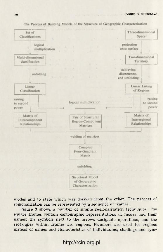
5 2 i B O R I S B . R O D O M A N
modes and to state which was derived from the other. The process of regionalization can be represented by a sequence of frames.
Figure 3 shows a number of simple regionalization techniques. The square frames contain cartographic representations of modes and their names; the symbols next to the arrows designate operations, and the rectangles within frames are regions. Numbers are used for regions instead of names and characteristics of individuums; shadings and sym-
http://rcin.org.pl

F O R M A L I Z A T I O N O F R E G I O N A L C H A R A C T E R I S T I C S 5 3
Fig. 3. The simplest techniques of single-level individual and typological regiona-lization
bols designate different classes. In addition, modes are designated by-capital letters and operations by small letters.
These regionalization techniques are, of course, not exhaustive. Soviet physical geographers, for example, often obtain IR (individual regionalization) by combining small typological regions. On Fig. 3, this operation would be represented by TP-+IR2, with microregions substi-tuted for the point symbols in mode TR.
Mode CR (classification of regions) is the simplest way of combining IR (individual regionalization) and TR (typological regionalization) on the same map. It can be regarded IR u TR if we think in terms of the set of points that make up the lines of a drawing. If we print the maps on transparent paper, we find that by superimposing IR on TR, we obtain CR, and that by superimposing IR, TR or both modes on CR, we do not change the external appearance of CR. The same applies to the point modes: CP~IP u TP. As is evident from Fig. 3, a chorogenic CR may contain adjoining regions of the same class, but a typological CR may not.
The listing of operations can be ordered and simplified if we regard them as consecutive or parallel combinations of such operations as the disjointing of sets, the union of subsets, the combination of a place sym-bol with a property symbol, the removal of symbols, etc.
http://rcin.org.pl

54 i B O R I S B. R O D O M A N
If we designate the volume of phenomena in the objective world, as reflected by mode M, as v, and those reflected by mode M' as v we can define three categories of operations M—>M' and can group the ope-rations shown in Fig. 3 in these three categories:
(1) the collection of new information (v<iv')\ s (description), i (indivi-dualization);
(2) regrouping of existing information (v — <Cv'): c (classification), dc (declassification);
(3) rejection of unnecessary information (v>v')\ di (disindividuali-zation).
A sequence of different categories of operations constitutes a cycle characteristic of any type of research. These cycles are evident in Fig. 3 (in the periodic alternation of the three types of arrows).
Operations (1) and (2), corresponding to the condition v ^ v ' , may be called reversible because they can be followed by the reverse movement M<-M' without the use of information not already contained in M. Ope-rations of category (3) are irreversible, as are all processes of carto-graphic generalization. There are also pairs of mutually reversible ope-rations: i and di, c and dc.
By dropping the last letters of the abbreviated designations of the regional and point modes, we can designate by arrows all the operations that may be performed without the use of information not already con-tained in the transformed mode:
These arrows indicate the paths in which material can be regrouped and reduced; this would be the procedure used by a person who compiles a map in the office without the possibility of supplementing available sources.
The diagnosing of objects, i.e. assigning them to classes of a pre-viously given classification based on a comparison of identified indi-viduums. Consequently the operations s (description), c (classification) and di (disindividualization) form a group (in the mathematical sense of the word), i.e. gf = s + c + di. The plus in this formula may be interpreted as the symbol of vector addition of paths in a discrete space, whose points correspond to different modes. The process of formalization of geography may find use for the theory of groups elaborated by Otto Yu. Shmidt, the outstanding Soviet geographer, mathematician and Arc-tic explorer (1891—1956). Mathematical investigation of logical and map--compilation operations, the application of the algebra of states and events could help us find ways of mechanizing and automating the process of regionalization.
http://rcin.org.pl

F O R M A L I Z A T I O N O F R E G I O N A L C H A R A C T E R I S T I C S 55
REGIONALIZATION AND THE THEORY OF GRAPHS
The theory of graphs is just as close to problems of regionalizationas is set theory. The theory of graphs has a bearing on regionalization at least in the following cases:
1. A network of boundaries between regions constitutes a plane multangular graph. Consequently different concrete regional networks can be studied topologically and described in terms of the theory of graphs.
2. If we place a point within each edge of a graph G and connect the points of adjoining edges by lines, we obtain a graph G* that is a dual of the original graph (see Ref. 2, pp. 100—102). This operation, known as inversion, has an interesting economic-geographic interpre-tation: by inverting a graph of economic nodal regions, we obtain a topo-logical scheme of communications, and by inverting the graph of the transport network, we obtain a scheme of regions that gravitate toward transport nodes.
3. Any graph can be replaced by an adjacency matrix which shows which vertices of a graph are connected and which are not. For a direc-ted graph, this would be a complete square matrix, and for a nonindi-rected graph it would be half the matrix, lying on one side of the main diagonal. In the other hand, the existence and absence of communica-tions between regions or points, as well as the direction of the communi-cations, can be expressed by a graph. A geographical interpretation of these facts is the above-mentioned interrelationship between regiona-lization and a matrix of interregional flows (see Section 4).
4. A multi-level classification or regionalization scheme can be repre-sented graphically by a graph in which the vertices correspond to taxons (regions or classes of a certain rank), and the arcs show the relationship of subordination and inclusion of the taxons. Such a graph can be called a taxonomic graph. We can differentiate two kinds of taxons: (1) abstract crete taxons, such as the province Yenisey Ridge or the species Siberian Spruce. A graph showing abstract taxons would be called a taxono-mic stairway, and a graph of concrete taxons a taxonomic pyramid. In contrast to the traditional forms of classification, a taxonomic graph can have cycles (Fig. 4).
5. A block diagram of the process of regionalization corresponds to a directed graph in which the vertices designate modes and the arcs operations (see Fig. 3), or, conversely, the arcs modes and the vertices operations. The scheme of the regionalization process and, in fact, the entire process of compilation of a geographic characterization (see p. 52) may take the form of a network graph in which the most timeconsuming
http://rcin.org.pl
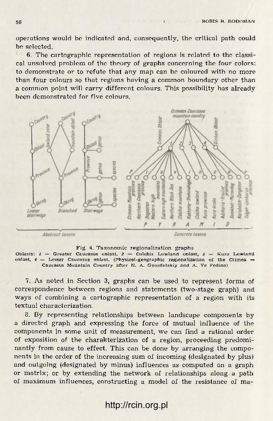
56 i B O R I S B. R O D O M A N
operations would be indicated and, consequently, the critical path could be selected.
6. The cartographic representation of regions is related to the classi-cal unsolved problem of the theory of graphs concerning the four colors: to demonstrate or to refute that any map can be coloured with no more than four colours so that regions having a common boundary other than a common point will carry different colours. This possibility has already been demonstrated for five colours.
Fig. 4. Taxonomic regionalization graphs Oblasts: 1 — Greater Caucasus oblast, 2 — Colchis Lowland oblast, 3 — Kura Lowland oblast, 4 — Lesser Caucasus oblast. (Physical-geographic regionalization of the Crimea =*
Caucasus Mountain Country after N. A. Gvozdetskiy and A. Ye Fedina)
7. As noted in Section 3, graphs can be used to represent forms of correspondence between regions and statements (two-stage graph) and ways of combining a cartographic representation of a region with its textual characterization.
8. By representing relationships between landscape components by a directed graph and expressing the force of mutual influence of the components in some unit of measurement, we can find a rational order of exposition of the charakterization of a region, proceeding predomi-nantly from cause to effect. This can be done by arranging the compo-nents in the order of the increasing sum of incoming (designated by plus) and outgoing (designated by minus) influences as computed on a graph or matrix; or by extending the network of relationships along a path of maximum influences, constructing a model of the resistance of ma-
http://rcin.org.pl

F O R M A L I Z A T I O N O F R E G I O N A L C H A R A C T E R I S T I C S 57
terial, of the strain in strong arcs and breaks in weak arcs; or, finally, by seking, if possible, the suitable Hamiltonian path, i.e. the line that passes throgh all the vertices of the graph once and only once. (These techniques are only suggestions by the author that have yet to be tested in practice).
9. Ey coding a graph of regionalization or of intercomponent rela-tionships with a linear succession of symbols, as is done in physical--chemical diagrams of the composition and properties of metal alloys (see Ref. 6), one could obtain the basic characteristics of the morpholo-gical structure of natural and agricultural landscapes suitable for ma-chine classification and rapid retrieval in a cadaster library, or as stan-darts for automatic diagnosing of landscape types.
There is evidently an infinite set of examples in which the theory of of the material world are more important and mundamental than the metrical properties. Topology, discreteness and whole numbers dominate in schemes that describe the structure of scientific knowledge. There-fore the representation of regionalization schemes, as well as schemes of relationships between regions and components of the geographic envlope, in the form of graphs may become one of the promising trends in mathematical geography.
REFERENCES
1. B. L., Gurevich, and Yu. G., Saushkin, The Mathematical Method in Geo-graphy, Vestn. Mosk. un-ta, ser. geogr. No. 1, 1966, (translated in Soviet Geography, April 1966).
2. O., Ore, Graphs and Their Uses, Random House, New York, 1963. 3. B. B., Rodoman, Methods of Individual and Typological Regionalization and
their Representation on Maps, Voprosy geografii, No. 39, 1956. 4. B. B., Rodoman, Logical and Cartographic Forms of Regionalization and their
Study Objectives, Izv. AN SSSR, ser. geogr. No. 4, 1965. 5. Yu. A., Shikhanovich, Vvedeniye v sovremennuyu matematiku (Introduction
to Modern Mathematics). Moscow, Nauka, 1965. 6. V. S., Shteyn, Solution of some Information Problems of Physical-chemical
Analysis with the Help of Electronic Computers (Summary of a dissertation for the degree of candidate of technical sciences), Moscow Chemical Technology Insti-tute, 1966.
7. B. J. L., Berry, Approaches to Regional Analysis: a synthesis, Ann. Assoc. Amer. Geogr., No. 1, 1964.
8. R. G., Golledge, and D. M., Amadeo, Some Introductory Notes on Regional Division and Set Theory, Profess. Geographer, No. 1, 1966.
http://rcin.org.pl

http://rcin.org.pl

G E O G R A P H I A P O L O N I C A 15
A FACTOR ANALYSIS APPROACH TO SUB-REGIONAL DEFINITION IN CHENANGO, DELAWARE, AND OTSEGO COUNTIES *
B A R C L A Y G . JONES a n d W I L L I A M W . G O L D S M I T H
The utilization of rural resources and the development of non-urban regions has attracted increasing attention in recent months. As techno-logical changes have dictated new locational patterns, the dislocations caused by transitions from one form of economic activity to another have been shown to result in an interrelationship of social, economic, and political problems. The recognition of the existence of these problems has occasioned a response from both public and private groups. Dr. Har-vey S. Perloff has called attention to this recent upsurge in activity and has cautioned us about the need for a more profound understanding of the situation as a foundation for remedial programs.
This is a field in which action programs seem to have grown at a much faster rate than the underlying knowledge essential to their effectivenness. Over 10,000
* The project received financial support jointly f rom research funds of the New York State College of Agriculture and the New York State Cooperative Extension Service at Cornell University. It was conceived, as mentioned, as part of a larger series of studies supported by those organizations and under the direction of Professors Conklin and Allee. Support and encouragement were given A.A. John-son, Clif ford R. Harrington and Harlan B. Brunsted of the Extension Service and W. Keith Kennedy of the College of Agriculture.
A number of people were interviewed and gave us information and advice on various aspects of the regional identification. We are particularly grateful for the help of the New York State Cooperative Extension Service personnel in the three-county region. They include: the County Agricultural Agents of the three counties, William E. Worth, Chenango; Paul G. Mattern, Delaware; W. Dale Brown, Earl S. Fineman, and William Gegenbach, Otsego; and the Home Demonstration Agents: Darlene F. Hecklenaible, Chenango, Linda Clark, Delaware; and Amelia D. Bielaski, Otsego.
The staff of the project consisted of the Director, Barclay G. Jones, and two Research Assistants, William W. Goldsmith and John T. Lang. They were assisted in statistical and graphic work by Mrs. Louise Hertz, David W. Sears, and Brian H. Ford. Typing and preparation of the final report were done by Mrs. Mary Adesso.
http://rcin.org.pl
60 B A R C L A Y G . J O N E S A N D W I L L I A M W . G O L D S M I T H
public and private agencies in the United States are concerned in one way or another with "area development" 1.
Much of this recent interest has focused on the Appalachian region of the eastern United States. A series of counties in upstate New York, chiefly along the southern border of the State, have been identified as having many of the characteristics of underdevelopment of the Appa-lachian region. Underutilized agricultural resources, large areas of unu-sed land, low levels of income, high levels of unemployment, and low levels of growth in many sectors of the economy and in many compo-nents of the population characterize these counties. Steps are being taken to initiate a number of broad, sweeping studies to assess the present state of activity, seek the causes for underdevelopment, and seek solu-tions to some of these problems. At Cornell, a series of such studies has been undertaken under the leadership of Professor Howard E. Conklin and Assistant Professor David J. Allee of the Department of Agricultural Economics of the New York State College of Agriculture at Cornell Uni-versity. This study was carried out as a part of the larger group of in-vestigations.
Basic to regional studies is the identification of the region to be investigated. Regional definition must always be flexible and related to the purposes of the study. As Dr. Joseph L. Fisher has reminded us in an article on regional definition, "At the outset, the general point should be made that the purpose which the analyst has in mind invariably governs the type of region he selects"2. He goes on to identify five general kinds of regions: the smaller economic region, the metropolitan area, the geographic or natural resource region, the region of admi-nistrative or data convenience, and the economic development region.
The three counties that have been selected for this study, Chenango, Delaware, and Otsego, form a reasonably homogeneous economic deve-lopment region in the southern central portion of New York State. By and large, the counties are surrounded by major transport routes but not crossed by them. Major urban areas surround the three-county region but are neither found in it nor penetrate it. The region contains the headwaters of the Susquehanna and Delaware rivers.
The purposes of the study, of which this report is a result, were to assess the present state of activity in the region and identify sectors of growth and decline, and to investigate the sub-regional differences among
1 Harvey S. Perloff, Edgar S. Dunn, Jr., Eric E. Lampard and Richard F. Muth, Regions. Resources, and Economic Growth, University of Nebraska Press, Lincoln, Nebraska, 1960, p. 3.
2 Joseph L. Fisher, Concepts in Regional Economic Development, Papers and Proceedings of the Regional Science Associaton, Vol. I, 1955, pp. W-3.
http://rcin.org.pl
FA.CTOR A N A L Y S I S A P P R O A C H T O S U B - R E G I O N A L D E F I N I T I O N 63
the areas that comprise the region. Treating a region as a single entity is extremely useful at certain levels of investigation. It can yield much insight and understanding about the fundamental problems of the region and can indicate the nature of solutions to them. However, if the region is of any geographical extent, it will be found to be made up of many component regions having characteristics of their own and many diffe-rent kinds of problems. Any attack on the problems of a region must consider the different types of subregions that comprise it and the spe-cific nature of their individual problems.
For example, within a single region one can find prosperous urban areas, wealthy suburbs, urban slums, developed urban-fringe areas, pros-perous agricultural sections, and poor rural slums. The over-all indices for such a region might suggest that the development process was going along at a reasonable pace. However, closer examination might indicate that some areas are progressing extremely rapidly while actual deterio-ration of the situation prevails in other sub-sections.
Action programs are usually directed at specific problems. It is im-portant to identify sub-areas within a region in which these problems exist to provide a focus for such programs. Sub-regional analysis can also serve to identify problem areas in regions for which the over-all indices do not indicate the existence of such problems.
During the summer of 1965 we undertook a research project directed at both of these objectives. The results of the investigation are contained in two companion reports: this and one entitled, Studies in Regional Development: Population, Activities, and Income in Chenango, Delaware, and Otsego Counties. The latter report is concerned with the present state of activity in the region and the analysis of sectors of growth and decline. This report deals with our attempts to identify sub-regions within the study area.
THE PROBLEM
S U B - R E G I O N A L I Z A T I O N
As the casual traveler drives through Chenango, Delaware, and Otsego Counties, perhaps tracing an easterly route through the Sus-quehanna Valley, he is struck by the general similarity of the villages, valleys, hills and countryside through which he moves. However, if the traveler decides to stay a while in the area, or if he makes frequent sub-sequent visits, he cannot help but be struck by the wide range of expe-riences he has. While the general structural identity of the region remains as a strong impression, a rich variety of differences becomes apparent.
http://rcin.org.pl

62 B A R C L A Y G . J O N E S A N D W I L L I A M W . G O L D S M I T H
The region always seems to offer something new to observe as it reveals more and more facets of its nature upon closer scrutiny. The valleys that at first glace seemed very similar, upon longer acquaintance are set apart from each other as their characteristics are perceived. The small country villages that, at first, seemed so much of one size, period, and type, on greater familiarity are seen to have richly varied personalities. Differences in the rural landscape become apparent from section to section too.
The analyst has much the same series of experiences as the traveler. The essential homogeneity, unity, and relative self-sufficiency of the region is the most striking fact at first. The region's relative isolation from other areas and its strong linkages and interdependencies within itself loom very importantly. However, as the study proceeds, the ana-lyst too becomes increasingly aware of the diversity and variety of the sub-areas composing the region. The more deeply he goes into his inve-stigation, the more differences appear.
It can be argued that this dual pattern is of the essence of regional studies. In the first instance, the regional analyst is concerned with dis-covering the identity of his region. This identity is defined in terms of the characteristics which set it apart from other regions and differen-tiate it from the rest of the world. However, the analyst must also dis-cover the nature of his region. This requires that he understand the elements that comprise it and that he become aware of their variety, diversity, and interdependence. Compositional differences are of the es-sence of regional identity also. They can be defined in two ways. Units are sometimes distinguished from each other because of the different elements that comprise them. More often the classification of types of units is dependent upon different mixes of similar elements. In regional analysis, the latter kind of differentiation is often more important although the former plays a larger role.
Differences in regional composition are often treated in terms of aggregations of individual elements. For example, regions will be com-pared by differences in composition of such things as age and sex co-horts, occupational classification of the labor force, employment by in-dustrial sectors, and so forth. Another way of approaching the subject is to hypothesize that the aggregate differences characterizing regions being compared are, perhaps to a major extent, the result of different compositional mixes of various sub-areas that comprise them. Followed to one possible conclusion, one might hypothesize that working with a small enough geographical unit one could identify a finite set of n different kinds of sub-areas to be found, say, in the United States. For the purposes of analysis, all of the elements of any sub-set would be
http://rcin.org.pl

F A . C T O R A N A L Y S I S A P P R O A C H T O S U B - R E G I O N A L D E F I N I T I O N 63
considered identical wherever found. The differences between larger regions would then be defined in terms of different compositional mixes of sub-sets.
For many kinds of action programs, this definition of regional diffe-rences could be very useful. Most area-oriented action programs are directed at specific kinds of problems. Sub-set areas could be defined in relation to these problem identifications. The application of these action programs would then become area specific within the regions in which they were mounted.
How the analyst can make himself familiar with sub-regional diffe-rentiation within the constraints of his study is a problem that has long been recognized. Sir Patrick Geddes, one of the earliest scholars of re-gions, was fully aware of the fact that we must know a region well to distinguish it from other regions and to identify the sub-areas that com-prise it. Unless we know it this well, our studies are not likely to serve as the basis for appropriate action to assist the region. He felt the re-gional scholar should become intimate with the area he was studying and inhabit it for a considerable period of time before he could say anything meaningful about it.
Still, more must we take our share in the life and work of the community if we would make this estimate active one; that is if we would discern the possi-bilities of place, of work, of people, of actual groupings and institutions or of needed ones, and thus leave the place in some degree the better of our life in it; the richer, not the poorer, for our presence 3.
Certainly, first hand familiarity is extremely desirable. Specific pro-grams requiring major changes involving human beings or large expen-ditures of money require intimate knowledge of the particular circum-stances. However, firsthand knowledge is not sufficient in itself. Often fresh approaches by outsiders serve as necessary catalysts to help in-dividuals who are too intimately aware of local situations to perceive problems in new ways and seek new solutions. Because analysts and administrators dealing with large regions cannot become intimately fa -miliar with every aspect of all of the sub-areas with which they are con-cerned, short cut methods must be found. The problem that concerned us in this study was to explore the usefulness of various analytical me-thods and techniques for scrutinizing a region rapidly for the purpose of screening out different kinds of sub-areas that comprised it.
The region we are concerned with contains about 3400 square miles of area and 139,000 people and their activities. Our analysis, which
3 Sir Patrick Geddes, Cities in Evolution, new and revised edition. Jaqueline Tyrwlhitt (ed.), Williams and Norgate, Ltd., London, 1949; p. 112.
http://rcin.org.pl

64 B A R C L A Y G . J O N E S A N D W I L L I A M W . G O L D S M I T H
yielded us a great deal of information about this area, these people, and their activities, was reported in the companion document cited earlier 4. It became quite clear through that analysis that no one set of generaliza-tions was sufficient to describe the population and activities of the re-gion, but that it was necessary to define sub-regions within the area and to treat them differently.
To identify the nature of region, we had to aggregate and summarize the available information. On the other hand, we had to break the region into sub-areas to understand it more fully. Much of the information that was gathered, analyzed, and reported concerned sub-divisions of the region. However, this information is difficult to use both because of its amount and its complexity. To make the sub-regional information meaningful, it is necessary to group and summarize so as to be able to generalize about types of sub-areas that comprise the three-county region.
To generalize about sub-regions, it is necessary to classify observa-tional units with like characteristics together. The first question con-cerns the selection of the basic areal unit. The smaller the initial areal units, the more internally homogeneous we can expect them to be. The more homogeneous they are, the more meaningful will be the sub-sets into which we group like units. However, the smaller the areal unit, the less information available. Reporting and sampling errors also be-come magnified as we work with smaller units. A compromise between internal homogeneity and information availability and accuracy must be made.
In many cases, the nature of the problem will be dictated somewhat by the situation being studied. In the three-county region with which we are concerned, data are reported for only two sets of exhaustive sub-regions: the counties themselves and the minor civil divisions. For most purposes, the counties are so large in comparison to the region that they do not represent useful sub-regions. The 66 minor civil districts are composed of two cities and 64 towns. They are the smallest units for which much information is available that cover the entire region. The number of units is sufficiently large to make possible considerable discri-mination of sub-areas within the region. However, much interesting and relevant data are not available for minor civil districts.
Since the advantages of the minor civil districts were clearly su-perior to any other elementary unit, they were chosen for purposes of
4 Barclay G. Jones and Jon T. Lang, Studies in Regional Development: Po-pulation, Activities, and Income in Chenango, Delaware, and Otsego Counties. Di-vision of Urban Studies, Cornell University, October, Ithaca, New York, 1965.
http://rcin.org.pl
FA.CTOR A N A L Y S I S A P P R O A C H T O S U B - R E G I O N A L D E F I N I T I O N 67
observation. In New York State, towns are relatively uniformly-sized subdivisions of counties. They may contain cities, villages, unincorporated urban places, and rural land. They are units of collection and reporting of many data by Federal and State agencies and are quite amenable to statistical comparison and analysis.
The lack of information and unreliability of some of the sample data for such small units present problems which are considerable. Much information commonly available for larger areas such as cities, metro-politan regions, and counties, is not available for minor civil divisions. Other information which might be useful for analysis is not available because of a large number of zero readings for many of the units. In other words, some phenomena simply do not occur in many minor civil di-visions.
The specific problem then becomes one of finding a methodology which will use data readily available for minor civil divisions and that will group them usefully into more or less homogeneous sub-regions. If the method of procedure is to be useful to other scholars elsewhere, it seems important to confine the data to readily available published or unpublished sources. Furthermore, these data must be quantifiable in standard terms. The procedure would seem to be to gather available quantified data relevant for purposes of regional classification for each of the 66 minor civil divisions. The characteristics of the elementary units should then be compared in such a way that they can be grouped into fewer than 66 sub-regions but more than a single region. Several methods of analysis are available for this sort of sub-regional delineation. All of the methods have similar information requirements but some seem to make better use of the information than others.
Probably the simplest and most common sub-regional delineation is that made by direct observation and subjective classification. Sub--regions arrived at in this manner might be useful but it is possible that they would neglect important information. The data presented might be so numerous that they could not be adequately reviewed and unavoi-dable biases of the investigators would come into play as the data are subjectively sorted. The methods would derive sub-regions which would not be reproducible or directly comparable to those arrived at by other kinds of approaches.
A somewhat more rigorous approach would use more or less simple processes of sorting on the values of the variables. This might involve the scaling of each variable in categories, perhaps just high and low, or perhaps in a larger number of class intervals. It might even prove to be more useful to group similar variables in linear combinations and
5 G e o g r a p h i a P o l o n i c a t. 15 http://rcin.org.pl
68 B A R C L A Y G . J O N E S A N D W I L L I A M W . G O L D S M I T H
conduct a scaling on the combinations. One of the most rigorous and efficient methods of doing this is factor analysis.
After any scaling procedure, it becomes necessary to try to identify regions with similar scores on a number of variables or combinations of variables. This can be done by a number of methods such as contingency tabling or direct distance scaling 5.
Basically, the problem reduces to finding a consistent and easily usable method whereby the values of a number of characteristics of small geographical units may be compared so as to classify these units into groups which will comprise meaningful and useful sub-regions within a larger region under study. Such a method then could be applied in a number of different regions for different purposes. If the variables are appropriately chosen and if the method is successful, the results should be some sort of first approximation of the composition of regions in terms of identifiably different sub-regions. It would then be advisable to confirm the results in the field to determine whether or not the sub--regions relate to the purposes for which the analysis was carried out. Further refinement of the regional definition will probably be necessary as a basis for various kinds of action programs. However, the method will have permitted analysts or administrators concerned with far larger and more complex areas to focus their attention much more sharply on the specific kinds of areas in which they are most interested.
T H E T H R E E - C O U N T Y R E G I O N
A report on sub-regional definition of an area with which the reader is not familiar seems of marginal value. The reader has no basis for judging the usefulness of the method or the validity of the results. It seems appropriate to describe briefly some of the major characteris-tics of the three-county region to provide a background that may be helpful in reviewing the results of the analytical study.
The compact, almost circular, three-county region formed by Che-nango, Otsego, and Delaware Counties is approximately centered on Oneonta. It lies in the southern portion of New York touching the Penn-sylvania boundary somewhat east of the center of the state. While upstate metropolitan areas such as the Capital District, Utica-Rome, Syracuse, and Binghamton surround it at some distance on all sides the
5 Brian J. L. Berry, A Method for Deriving Multi-Factor Uniform Regions, Przegląd Geograficzny, Vol. 33, No. 2, 1961, pp. 263—279. Here Berry computes the equivalent of the hypotenuse between two points measured in n-dimensional space.
http://rcin.org.pl

F A C T O R A N A L Y S I S A P P R O A C H T O S U B - R E G I O N A L D E F I N I T I O N 317
region does not contain a major urban center. Federal highways U.S. 11 and U.S. 20 skirt the region as do Interstate Routes 81 and 95. The major roads serving the region are N.Y.S. 12 and 7 which traverse it and N.Y.S. 17 which crosses the southern boundary on its way between Binghamton and New York City.
The region occupies most of the eastern portion of the Plateau Country of southern New York. The plateau is bounded on the south by the Delaware Hills and the Catskill Mountains. The hills are almost
Fig. 1. Agricultural regions of central New York state Source: H. E. Conklin and E. E. Hardy, Map of Agricultural Regions of New York State
(Ithaca, New York, New York State College of Agriculture at Cornell University, 1963)
entirely contained in the region and the Catskills border it penetrating it slightly at a couple of places. To the north the plateau drops sharply away in the Escarpment Country to the Mohawk River Valley. Figure 1 shows the agricultural regions of southern-central New York giving the location of the three-county area.
The western portion of the region is characteristic of the relatively flat but rolling highlands of the Plateau Country. Shallow valleys traverse it providing accent to the countryside. As the plateau progresses eastward, the hills rise higher and the valleys cut deeper and, in most cases, more narrowly. At the northern edge of the region, the plateau falls off sharply through the escarpment country to the Mohawk River Valley.
6* http://rcin.org.pl

68 B A R C L A Y G . J O N E S A N D W I L L I A M W . G O L D S M I T H
The drop is 1|000 to 1500 feet in a distance of 10 miles or less with 1000-foot drops in distances of 1 mile or less at some places. At various points along the northern boundary there are splendid panoramic views across the valley. To the southeast, the plateau gives way to the sharper undulations, steeper slopes, and narrower valleys of the Delaware hills. The landscape is substantially more dramatic and some of these sharply defined valleys provide wonderfully picturesque scenes. Further to the southeast the Delaware hills continue to rise until they finnaly merge into the noble forms of the Catskill Mountains.
The general topographic features of the three-county region are shown in Fig. 2. Here, the increasing hilliness and the increasing ele-vations in the eastern sections can be seen. Also apparent is the system of valleys which, in essence, provides the topographical structure of the region. These valleys drain south and west and belong to two great watersheds: the Susquehanna and the Delaware. The East Branch and the West Branch of the Delaware River provide two central valleys run-ning from the northeastern to the southwestern part of Delaware County. The East Branch of the Delaware is the lesser of the streams and has the narrower valley. Route N.Y.S. 30 traverses it connecting the major settlements of Honcock, Downsville, Margaretville, and Fleischmanns. The central portion of this valley is now occupied by the Pepacton Reservoir.
The valley of the West Branch of the Delaware provides the central organizing element of Delaware County. Route N.Y.S. 10 connects the communities that lie in this valley: Deposit, Walton, Delhi and Stamford. The Cannonsville Reservoir lies between Deposit and Walton. The valley is steep and picturesque and contains some of the handsomest com-munities in the region.
The valley system of the Susquehanna and its tributaries is, and has always been, a more important structural factor in the region than the Delaware. The Otselic River and its valley penetrate slightly into the northwest corner of the region. This stream joins the Chenango River just before it flows into the Susquehanna at Binghamton. The Chenango River Valley is broad and fertile. It traverses Chenango County from the north to the southwest corner. The Erie-Lackwanna Railroad and Route N.Y.S. 12 run through the valley connecting Binghamton and Utica-Rome. The Chenango Canal used to run up the valley to the north to join with the great Erie Canal system. Most of the major communities in Chenango County are found in this valley: Greene, Oxford, Norwich and Sher-burne.
To the east there is a series of lesser streams coursing through north--south valleys to find their way into the Susquehanna. The most im-
http://rcin.org.pl

FA.CTOR A N A L Y S I S A P P R O A C H T O S U B - R E G I O N A L D E F I N I T I O N 69
portant of these is the Unadilla River which separates Chenango from Otsego Counties. Wharton and Butternut Creeks f low into it. Otego Creek lies farther east. These streams join the Susquehanna in a broad valley which runs down the center of the region from the northeast to the southwest. An important line of the Delaware and Hudson Railroad
Fig. 2. Topographic features, three-county region Source: U. S. Corps of Engineers, Army Map Service Topographic Map of Binghamton
area, 1950. Scale 1 : 250,000
connecting Binghamton with Albany runs through the valley as does Route N.Y.S. 7. The major transportation routes and the major urban settlements of the region lie in this valley. It contains the communities of Afton, Bainbridge, Sidney, Unadilla, Oneonta, and Cooperstown. This valley is the unifying link for the region and provides a focus for many of its activities. A system of small valleys at the eastern edge of Otsego County run southwesterly into the Susquehanna. Most of these are minor with the exception of that of Schenevus Creek which provides a trans-
http://rcin.org.pl

70 B A R C L A Y G . J O N E S A N D W I L L I A M W . G O L D S M I T H
port linkage across the Susquehanna watershed divide into Schoharie County and the Hudson River system. The population dot map shown in Fig. 3 gives some idea of the present pattern of human occupancy of the region. It is interesting to compare it to the topography.
Fig. 3. Population dot map, three-county region, 1960 Source: U. S. Bureau of the census, U. S. Census of Population, I960
The topographic features of the region are pronounced enough to have profoundly influenced the history of its development. In general the region is not mountainous but upland being at the headland of the plateau. Because it occupies a position at the very source of two major river systems, the streams are narrow, non-navigable, and occupy re-latively narrow valleys. In other words, the region has historically been comparatively inaccessible. The greatest agricultural potential has always been in the narrow valleys, and most of the intensive commercial farming that remains in the region is found in them. These farm lands are readily accessible to transport but, at the same time, agriculture must compete
http://rcin.org.pl

FA .CTOR A N A L Y S I S A P P R O A C H T O S U B - R E G I O N A L D E F I N I T I O N 7 1
:'or them with transport uses themselves and other activities that are dependent upon transport such as residence, commerce and industry.
The history of the region has been described in the companion volume cited earlier6. The historical pattern of development has largely fol -
Fig. 4. Generalized Soil Association map, three-county region Source: Martin G. Kline, Soils and Soil Associations of New York, Cornell Extension Bulletin 930 (Ithaca, New York, New York State College of Agriculture at Cornell University,
1963)
lowed that of agriculture as it was introduced into the region. Agricul-ture, in turn, was governed by topography and by the responsiveness of the soils to cultivation. Much of the historical development of the region can be explained by looking at the soils it contains. Many of the future
6 Jones and Lang, op. cit., pp. 9—13.
http://rcin.org.pl
72 B A R C L A Y G . J O N E S A N D W I L L I A M W . G O L D S M I T H
prospects of the region are dependent upon these soils also. Figure 4 shows in schematic fashion a soil association map for the three-county area. A closer look at the nature of these soils is rewarding in helping to explain the present state of development and to define some of the current problems in the region.
On the northern fringes of the region are found a number of soils that are more commonly associated with the plains, valleys, and escarpment country 7. These soils occur primarily in relatively small areas. Largest in extent is the Langford-Erie Association at the heads of the Chenango and Unadilla Rivers. These low-lime, strongly-acid, glacial-fill soils are moderately well drained. They seem best suited for corn, small grains, and hay. Along the northeastern edge of Otsego County is a small area of the Honeoye-Lima Association of soils. These deep, high-lime soils are generally well drained and are among the best soils in the State. Agriculture is, however, less successful on these soils at high elevation. In the northeast corner of Otsego County are soils of the Farmington and Shallow Honeoye and Nellis Association. These shallow soils cover limestone bedrock and are unsuited to cultivation.
Most of the region contains soils associated with the plateau. The most fertile soils in the area are those of the Chenango-Tioga and Ho-ward-Chagrin Association which occupy the valley floors of the region. They are well drained and have good water-holding capacity. They erode little and are well-suited to most agricultural crops. These productive soils are extremely important to the agriculture of the region.
In the western and northern part of the region, the Chenango-Tioga soils of the valley bottoms are surrounded by the Lordstown-Mardin--Volusia Association on the hills and minor valleys. They include well, moderately, and imperfectly drained soils. In many cases, they provide excellent upland soils but these are often remote from transport routes and agricultural populations.
Much of the western-central portion of Chenango County is occupied by soils of the Volusia-Mardin Association. Most of the slopes in this area are moderate and drainage is often an outstanding problem of this group of soils. To obtain moderate or possibly good production from these soils is costly compared with better-drained and more fertile ones. In the northeastern portion of Chenango County are the strongly-acid, well to moderately well-drained soils of the Bath-Mardin-Lordstown Association. While these soils are potentially productive, many of them
7 The following discussion is derived from Marlin G. Kline, Soils and Soil Associations of New York, Cornell Extension Bulletin 930, New York State College of Agriculture at Cornell University, Ithaca, New York, 1963.
http://rcin.org.pl
FA.CTOR A N A L Y S I S A P P R O A C H T O S U B - R E G I O N A L D E F I N I T I O N 75
are remote and inaccessible and have been abandoned. They are well suited to dairy crops and some vegetables.
Cutting an east-west swath from the center of Chenango County through Otsego into the center of Delaware County are soils of the Walton-Wellsborough Association. While these soils are deep in the valley bottoms, they are shallow on the upper slopes and hill tops over red shale and sandstone bedrock. As a result, the use pattern is such that the valleys and lower slopes are very productive in their support of dairy industry while the upper slopes and crests are forested.
Adjacent to the soils of this group, both to the north and the south, are those of the Lordstown Association. They are well to imperfectly drained and are dominated by steep, shallow soils. As a consequence, little agriculture is practiced and most of the area is forested.
In the extreme eastern section of the region along the southeastern boundary of Delaware County are the soils of the Oquaga Association. These shallow soils cover the steep hills and mountains over red shale and sandstone bedrock. Most of this land is uncultivable except that which is located in small valleys where there is seldom enough to sup-port a viable agricultural enterprise. As a result, forest covers most of this area.
The best agricultural soils in the three-county region are located in the valley bottoms. Other productive soils occupy a northeast, southwest band through the center of the region. The agricultural problems seem to be chiefly too small a supply of fertile soils, inaccessibility and remo-teness from transport, and the distribution of fertile soils in such small areas as to prevent the development of efficient, large-scale agricultural activity.
The terrain is sufficiently rugged so that the most usable agricultural soils are concentrated in the narrow valleys that are most suitable for other uses also. Transportation facilities, villages and cities, rural non--farm residences, commercial activities, and industrial establishments compete with agriculture to crowd into these ribbon-like areas. There is less competition for the remainder of the region.
METHODOLOGY
F A C T O R A N A L Y S I S
Obviously, the three-county region is unified by a number of common characteristics. However, at the same time, it is apparent that it is com-prised of a wide range of quite different types of sub-areas. The problem is to discover a technique which will permit us to look at a number of
http://rcin.org.pl

74 B A R C L A Y G . J O N E S A N D W I L L I A M W . G O L D S M I T H
characteristics of the human occupancy and the human activities of the region and classify it into meaningful sub-regions.
The existence of many different methods for approaching this pro-blem was discussed earlier. The large number of different kinds of activities in the region, the peculiarities of their spatial configuration, and the lack of dominance of any single activity or group made the problem seem to us rather complex. We decided a method that used a large number of variables would be most appropriate in our case. Because we wished to use Minor Civil Divisions as the unit of obser-vations, we also had a large number of observations. Factor analysis, followed by scaling and contingency tabling seemed the most promising and efficient path to take.
Factor analysis is a mathematical technique that, from a large initial number of variables, derives new variables, called factors, that represent or summarize small sets of the original veriables. Factor analysis ap-pears most appropriate for our problem because of several inherent properties and capabilities. Firstly, it is concise. It can summarize in a few factors much of the information originally contained in a large number of interrelated variables. Secondly, it can suggest or corroborate hypotheses about unidentified or unmeasurable variables, such as "qua-lity of environment". Thirdly, the technique is amenable to high speed, electronic computation, allowing vast amounts of information to be handled with ease. The properties of factor analysis have been well described by H. H. Harman.
The principle concern of factor analysis is the resolution of a set of variables linearly in terms of (usually) a small number of categories or "factors". This reso-lution can be accomplished by the analysis of the correlations among the variables. A satisfactory solution will yield factors which convey all the essential information of the original set of variables. Thus, the chief aim is to attain scientific parsimony or economy of description 8.
The origins of factor analysis are from the field of psychology and are generally credited to Charles Spearman, who, at the turn of the century, wished to test a psychological theory which postulated a single intelligence factor manifested in a number of measurable traits (variab-les), such as reading speed, numerical ability and the like 9. Probably the most prominent name in factor analysis since Spearman is L. L. Thurs-tone, also a psychologist10.
8 Harry H. Harman, Modern Factor Analysis, University of Chicago Press, Chicago, 1960, p. 4.
9 Charles Spearman, General Intelligence Objectively Determined and Mea-sured, American Journal of Psychology, Vol. 15 1904, pp. 201—293.
10 L. L. Thurstone, Multiple Factor Analysis, University of Chicago Press, Chi-cago, 1947. For bibliographical information about both Spearman and Thurstone, as
http://rcin.org.pl

FA.CTOR A N A L Y S I S A P P R O A C H T O S U B - R E G I O N A L D E F I N I T I O N 75
One should not infer, however, because it originated from, and for a long time had dealt mainly with, psychology, that factor analysis is a psychological theory. It is not. It is a statistical technique applicable to many fields of which psychology is merely one. Nor should it be as-sumed that factor analysis can be used only to discover fundamental or basic factors in a system. It can be used to present a composite picture of several variations for a population as well n .
The way in which factor analysis incorporates information into the factors can perhaps be best illustrated by means of an example. A port-ion of the information used in the present analysis is shown in Figure 5A. The standardized values 12 of four variables highly correlated with Factor I are shown for six illustrative minor sivil divisions in the region. Each of the variables is a partial index of urbanization, and each is in-versely related to Factor I. The scores for Factor I for each of the six communities are plotted in Fig. 5B. The rough relationship between each of the variables and the factor can readily be seen. For Norwich and Oneonta the variables all have quite high values, and the factor scores have their highest (negative, because of the inverse relationship) values also. For Lincklaen and Decatur the variables have lower scores, and the factor scores are at the positive extreme. For McDonough and Harpersfield the variables group around zero, and the factor scores are very small also.
Exact correspondence between the four variables and the factor does not appear because the factor is actually constructed of weighted values of all 44 variables. The four chosen are those on which the factor is most
well as about many others concerned with factor analysis, see Harmon, op. cit., pp. 459—460. Other important works available on the general method of factor analysis are: C. J. Adcock, Factorial Analysis for Non-mathematicians, Melbourne University Press, Carlton, Victoria, 1954; R. B. Cattell, Factor Analysis: An Intro-duction and Manual for the Psychologist and Social Scientist, Harper and Bros., New York, 1952; B. Fruchter, Introduction to Factor Analysis, D. Van Nostrand Co., Inc., Princeton, N. J., 1954; H. Hotelling, Analysis of a Complex of Statis-tical Variables into Principle Components, Journal of Educational Psychology, Vol. 24, 1933, pp. 417—441, 498—520. For the general application to sub-regional defi -nition see M. J. Hagood and D. O. Price, Statistics for Sociologists, Henry Holt, New York, 1952, Chapter 26.
11 R. E. Granda, Introduction to Factor Analysis, (mimeographed Second Issue Revised, Cornell Computing Center, Ithaca, N. Y., July 1965.
12 The standardized value equals (observed value — mean value) / standard X X deviation, i.e., where X=observed value of the variable, X = t h e average
s
observed value, and s = the sample standard obser-
vations.
http://rcin.org.pl

76 B A R C L A Y G . J O N E S A N D W I L L I A M W . G O L D S M I T H
Fig. 5. Relationships, four selected variables and factor I
heavily weighted; four more variables, not used in the illustration, con-tribute substantially to the variation in the factor scores; the other 36 variables have weightings of approximately zero on Factor I. Had more variables been graphed in Fig. 5A the correspondence would have in-creased, but visual interpretation would quickly become more complex.
The summarization of the variables into the factor is accomplished by deriving factor loadings and computing factor scores. That is, the analysis arrives at a set of equations of the general form:
F j = l f r Z j i (1) i
or, more specifically,
Fj =h • Zji +fi • Zji +h •ZJ3 +... +fn• ZJn. (2)
http://rcin.org.pl

FA.CTOR A N A L Y S I S A P P R O A C H T O S U B - R E G I O N A L D E F I N I T I O N 77
Here Fj is the factor score for the jth unit of observation (minor civil division). It indicates how high or low the unit is rated on that parti-cular factor (illustrated by Figure 5B). The factor score is equal to the sum of the products of the factor loadings, f, times the standardized variables, Z. The factor loadings indicate the degree to which the parti-cular factor is associated with each of the variables being used.
The mechanics of the analysis depend only upon one set of infor-mation, the measure of association between pairs of variables, their intercorrelations. No other information about the variables is used13. In Table 1 a correlation matrix with such information for four variables is shown. In each cell is the simple correlation between a pair of var-iables, and the six correlations shown account for all pairs.
Table 1
Correlation matrix, four illustrative variables Variable
1 1 2 3 4
1 1.00
2 1 .21 1.00
3 1 -.12 -.28 | 1.00 4 1 .06 .14 | -.08 1.00
A single factor can be constructed to represent these four variables 14. It is derived from the correlations and its equation is
Fj = 0.3 Zn + 0.7 Zj2 - 0.4 Zj3 + 0.2 Zj4 (3)
Loadings are conventionally listed in Table 2. The correlations are pro-ducts of the factor loadings. For example, the correlation between vari-ables one and two, 0.21, is the product of the loadings for variables one and two (0.3X0.7 = 0.21). It can quickly be seen that all other correlations in Table 1 can be reproduced similarly.
Diagramatically, the factor and the variables can be represented as in Fig, 6. The circle represents the factor and the squares the variables.
13 Summarizing the data in a correlation matrix necessitates the assumption that knowledge of the second order moments (variances and covariances) uniquely determines all the information in the data, and this necessitiates the assumption that there is a normal distribution for the variables. See H. Solomon, A Survey of Mathematical Models in Factor Analysis, Part 3 in H. Solomon, Mathematical Thinking in the Measurement of Behavior: Small Groups, Utility, Factor Analysis, Free Press, Glencoe, 111., 1960.
14 For other, and more detailed examples along this line see Adcock, op. cit., and Walter Isard, Methods of Regional Analysis, The MIT Press, Cambridge, Mass., 1960, pp. 293—305.
http://rcin.org.pl
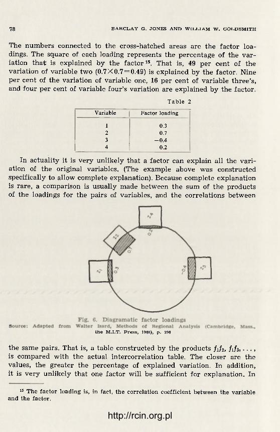
7 8 B A R C L A Y G . J O N E S A N D W I L L I A M W . G O L D S M I T H
The numbers connected to the cross-hatched areas are the factor loa-dings. The square of each loading represents the percentage of the var-iation that is explained by the factor15 . That is, 49 per cent of the variation of variable two (0.7X0.7 = 0.49) is explained by the factor. Nine per cent of the variation of variable one, 16 per cent of variable three's, and four per cent of variable four's variation are explained by the factor.
Table 2
Variable Factor loading
1 0.3 2 0.7 3 - 0 . 4 4 0.2
In actuality it is very unlikely that a factor can explain all the vari-ation of the original variables. (The example above was constructed specifically to allow complete explanation). Because complete explanation is rare, a comparison is usually made between the sum of the products of the loadings for the pairs of variables, and the correlations between
t h e M . I . T . Press , 1960), p. 296
the same pairs. That is, a table constructed by the products fj2, /1/3,.. . , is compared with the actual intercorrelation table. The closer are the values, the greater the percentage of explained variation. In addition, it is very unlikely that one factor will be sufficient for explanation. In
15 The factor loading is, in fact, the correlation coefficient between the variable and the factor.
http://rcin.org.pl

FA.CTOR A N A L Y S I S A P P R O A C H T O S U B - R E G I O N A L D E F I N I T I O N 79
the case where more than one factor is derived, the products of the lo-adings are, in effect, summed to be compared with the actual cor-relations.
So, the final product of the factor analysis itself is a set of factors, each of which explains some part of the original variation. The degree to which the factors explain the original variation is indicated by the divergence between the sums of the products of loadings and the ob-served intercorrelations among the variables. The correlation of any factor with any variable is the factor loading for the respective pair.
Actual methods of computation of the factor loadings are beyond the scope of this report. While the above discussion given a fair idea of what factor analysis is intended to do, it by no means tell how it does it. For more detailed explanation and for methods of computation and esti-mation the reader should consult the standard works mentioned in foot-note 3 above.
THE USE OF FACTOR ANALYSIS FOR SUB-REGIONAL IDENTIFICATION
The solutions to the problems for which factor analysis was originally developed required the grouping together, or classification, of similar but not identical individual observations. The characteristics of the indivi-dual observations were determined by the values of a large number of different kinds of attributes or variables. The existence of such problems in the field of psychology is obvious, and similar problems occur in other fields also. In the 1930's, there was a resurgence of interest in regional studies in the social sciences, particularly at such places as the University of North Carolina. The basic question of the identification of the region to be studies immediately arose.
Regions, like human beings, are never identical when viewed in any detail. Their characteristics are measured by means of long lists of vari-ables describing their populations and economies. They can be classified only by sorting them out into groups that have roughly similar characte-ristics. Factor analysis seems an appropriate tool to bring to bear on the problem of regional identification, and early attempts to use it for this purpose were made at the end of the 1930's.
Some of the earliest work using factor analysis as a technique for subregional delineation was done by Hagood, Danilevsky, and Beum 16. Their work was a preliminary exercise constructing a single factor for
16 Margaret Jarman Hagood, Nadia Danilevsky and Corlin O. Beum, An Exa-mination of the Use of Factor Analysis in the Problem of Sub-regional Delineation, Rural Sociology, Vol. 6, 1941, pp. 216—233.
http://rcin.org.pl

82 B A R C L A Y G . J O N E S A N D W I L L I A M W . G O L D S M I T H
five variables for Ohio counties. Two of the variables were longitude and latitude, used to force the resulting index to associate contiguous counties -closely. The index loadings were determined using Hotelling's method of iteration, and subregions of groups of counties were derived by scaling of scores of the single factor.
Dr. Hagood subsequently studied the patterns of some agricultural and demographic variables for the forty-eight states in order to arrive -at several groups of contiguous states, each group being internally ho-mogeneous with respect to the variables studied 17. Principle component analysis was used for the construction of indices for states, and states with like scores were grouped.
Also in 1942, Price published a factor analysis studying variation among the 93 largest cities in the 1930 U.S. Census 18. Price measured 15 characteristics for the cities and constructed four factors: degree of ma-turity, the extent to which the city is a service center, the general stan-dard of living, and the per capita trade volume.
In 1960 Hattori, Kagaya and Inanaga 19 investigated the area within a 40 km radius around the center of Tokyo. Sixteen indices were redu-ced by factor analysis to four factors indicating levels of urbanization, residentialization, industrialization and agriculture. An analysis of the structure of the region was made.
In 1961 Berry looked at 43 variables for 95 countries throughout the world and through factor analysis found that the original variables collapsed into four pattern explaining the more than 90% of the original variation20. Original variables related principally to transportation, energy, agriculture, communications, Gross National Product, trade and demography. The variables degenerated into four factors, the first two of which are called "technological scale", and "demographic scale". The
17 Margaret Jarman Hagood, Statistical Methods for Delineation of Regions Applied to Data on Agriculture and Population, Social Forces, Vol. 21, 1943, pp. 287—297.
18 Daniel O. Price, Factor Analysis in the Study of Metropolitan Centers, Social Forces, Vol. 20, May 1942, pp. 449—455.
19 Keijiro Hattori, Kaquyoshi Kagaya and Sachie Inanga, The Regional Struc-ture of Surrounding Areas of Tokyo, Geographical Review of Japan October 1960, pp. 495—514 (An English summary of the articles appears on pp. 513—514).
20 Brian J. L. Berry, Some Relations of Urbanization and Basic Petterns of Economic Development, in Forrest R. Pitts (ed.), Urban Systems and Economic Development, School of Business Administration, University of Oregon, Eugene, Oregon. June 1962, pp. 1—-15. For a more complete coverage of this analysis see Bery, An Inductive Approach to the Regionalization of Economic Development, in N. S. Ginsburg (ed.), Essays on Geography and Economic Development, Depart-ment of Geography Research Paper No. 62, University of Chicago Press, Chicago, 1960, pp. 78—107.
http://rcin.org.pl

FA.CTOR A N A L Y S I S A P P R O A C H T O S U B - R E G I O N A L D E F I N I T I O N 8 1
countries were mapped according to their quintiles on the two factor scores. The countries varied universely on the two factors, and the array of the countries on a scatter diagram of factor one and two scores is called a scale of economic development, which was found to be highly correlated with degree of urbanization
Aslo in 1961 Berry published an example of the use of factor analysis for the nine census divisions of the United States 21. Six original variables were reduced to two or three factors which explain most of the variance of the original six. The factors were analyzed by "distance scaling of similarities", which grouped the observations into homogeneuos re-gions 22.
Berry's example, using six original variables from which three impor-tant factors are derived, is, of course, oversimplified; but this oversim-plification coupled with the fact that the variables vary together to a large degree (they are density of service establishments for nine kinds of services) allows the direct scaling of similarities of result in a single, sensible regional pattern. The use of more diversified variables would clearly make the job of identifying one pattern of regions more com-plicated, if not impossible.
Moser and Scott23, also in 1961, reported on a statistical study using factor analysis to examine the social and economic differences of British towns. The study concerns all the 157 towns in England and Wales with 1951 populations over 50,000. Four major factors were extracted from 60 variables in the analysis: Social Class, Population Change 1931—51 and 1951—58 (together called Town's Stage of Development), and Over-crowding. Sljightly over 60% of the original variation was explained by these factors.
In 1962 H. Thompson, et al. suggested that "Factor analysis produces useful results when several indicators are handled simultaneously, and provides a logical basis for presenting spatial variation in economic health 2i. Dissatisfied with the disparate results from reasonable indica-
21 Berry, A Method . . . , op. cit. 22 Squared algebraic distances between factor scores are summed for each
pair of observations to give the squared distance between the observations (the square of the hypoteneuse). Observations with the most similar scores (least dis-tances) are successively grouped. The result is a tree of the nine census divisions which begins with "All U.S.A." and breaks down finally to the nine individual observations.
23 C. A. Moser and Wolf Scott, British Towns: A Statistical Study of Their Social and Economic Differences, Center for Urban Studies, Report No. 2, Oliver and Boyd, Edinburgh, 1961.
21 John H. Thompson, Sidney C. Sufrin, Peter R. Gould and Marion A. Buck,
6 G e o g r a p h i a Polonica t. 15 http://rcin.org.pl

82 B A R C L A Y G . J O N E S A N D W I L L I A M W . G O L D S M I T H
tors of economic health such as unemployment and per capita income the authors wished to arrive at a composite measure. Factor analysis allowed useful interpretations to be made.
In 1964 an elaboration of Berry's Przegląd Geograficzny scheme was applied by Ray and Berry in a socio-economic regionalization of Central Canada25. Each of 88 variables was observed for 120 areas, principle component factor analysis was used, supplemented by an orthogonal rotation using the varimax criterion to approach Thurstone's simple structure, and the resulting factor scores were subjected to distance scaling of similarities. The analysis was done for several large sub-groups of observations as well as for the entire 120 observations at once.
In 1964 Clavel attempted to summarize the variance of 20 social and economic variables for 64 census tracts in Syracuse, N. Y. 2 6 He pro-posed that residential location could be explained by level of amenities at a particular site, and the social and economic measures would indicate distinct areas. Factor analysis was useful as a descriptive summarizing device, and areas of the city with joint occurrence of certain high factor scores were mapped.
Schmid and Tagashira, in 1964, wished to utilize rigorous analytical tools to describe concisely the ecological and demographic structure of the large, urban community 27. 42 variables were measured for 115 census tracts for the city of Seattle. A principle axis solution was used and the factors rotated using the varimax criterion.. Four factors were felt by the analysts to be significant. They were family status, economic
Toward a Geography of Economic Health: The Case of New York State, Annals of the Association of American Geographers, Vol. 52, No. 1, March 1962, pp. 1—20.
25 D. Michael Ray, and Brian J. L. Berry, Multivariate Socio-Economic Regio-nalization: A Pilot Study in Central Canada (paper read at the Canadian Political Science Association Conference on Statistics, Prince of Wales College, Charlotte-town, Prince Edward Island, June 13—14, 1964). See also, Berry, Cities as Systems within Systems of Cities, in John Friedmann ad William Alonso (eds.), Regional Development and Planning, The MIT Press, Cambridge, Mass, 1964, pp. 116—137. In a subsection called Innovation Under Technical Impetus: Social Area Analysis, Berry covers "the new empiricism of the decade, stimulated by advancing computer technology and consequent diffusion of multivariate analysis throughout the social sciences''. He focuses on factor analysis as one form of multivariate analysis and briefly reviews "how, in the form of social area analysis, it has facilitated studies of the internal structure of cities". Berry mentions how factor analysis facilitates rigorous use of social area analysis for testing hypotheses of urban form, e.g., the Hoyt and Burgess theories.
26 Pierre Clavel, Behavioral Indicators of Residential Location Goals i Syra-cuse, New York, (Unpublished Paper, Cornell University, 1964).
27 Calvin F. Schmid and Kiyoshi Tagashira, Ecological and Demographic In-dices: A Methodological Analysis, Demography 1964, Vol. 1, 1964, pp. 194—211.
http://rcin.org.pl

FACTOR ANALYSIS APPROACH TO SUB-REGIONAL DEFINITION 317
status, maleness or sex status, and ethnic status. The scores for the iactors were trichotomized by several methods and mapped as high, me-dium, and low values for the census tracts.
An even more recent use of factor analysis for subregionalization will soon appear in Fisher's book on historical regionalization of the Yugoslav economy 28. The purpose of this use of factor analysis was to analyze the spatial impact of a particular set of postwar policies on urban structure, economic development, and urban migration. Significant differences in present level of social and economic activity were expected to reflect past foreign hegemony, and factor analysis was used to demon-strate this by deriving internally homogeneous subregions within Yugo-slavia. The results of the analyses of 55 urban centers and 611 communes for 26 variables provide substantial evidence that the country's various levels of development and activity are results of the geographical distri-bution of past foreign influence.
FACTOR A N A L Y S I S OF THE THREE-COUNTY REGION
The usefulness of factor analysis as a tool for subregional definition seems to have been clearly established. Its relevance to the problem confronting us in the three-county region seemed apparent. We wished to establish whether or not distinctive sub-regions existed and could be defined using data available for Minor Civil Divisions.
The final selection of basic units resulted in 66 observations for each of 44 variables. For simplicity the eight digit Minor Civil Division iden-tification code of the Bureau of the Census was used 29. This resulted in 20 towns, one city (Norwich), and one town remainder (Norwich) for Chenango County; 19 towns for Delaware County; and 23 towns, one city (Oneonta), and one town remainder (Oneonta) for Otsego County. Although there is some information for villages, there is far less than for towns and cities. There is even less information available for hamlets and other urban places. A list of the Minor Civil Divisions used as units of observation appears in Table 3.
The towns that comprise the region are roughly comparable in size, although the smallest, Decatur, in Otsego County, is only 21.4 square
28 Jack C. Fisher, Yugoslavia — A Multinational State: Regional Variation and Political Response (forthcoming).
29 See U.S. Department of Commerce, Bureau of the Census, Geographic Iden-tification Code Scheme: 1960 Census of Population and Housing. The twelve digit code allows identification of villages, but this level of detail was not useful for our analysis.
6* http://rcin.org.pl

86 B A R C L A Y G . J O N E S A N D W I L L I A M W . G O L D S M I T H
Table 3
Minor civil division identification scheme
Chenango County | Delaware County Otsego County
No. Town No. Town No. Town
1 Afton 23 Andes 42 Burlington 2 Bainbridge 24 Bovina 43 Butternuts 3 Columbus 25 Colchester 44 Cherry Valley 4 Coventry 26 Davenport 45 Decatur 5 German 27 Delhi 46 Edmeston 6 Greene 28 Deposit 47 Exeter 7 Guilford 29 Franklin 48 Hartwick 8 Lincklaen 30 Hamden 49 Laurens 9 McDonough 31 Hancock 50 Maryland
10 New Berlin 32 Harpersfield 51 Middlefield 11 North Norwich 33 Kortright 52 Milford 12 Norwich City 34 Masonville 53 Morris 13 Norwich 35 Meredith 54 New Lisbon 14 Otselic 36 Middletown 55 Oneonta City 15 Oxford 37 Roxbury 56 Oneonta 16 Pharsalia 38 Sidney 57 Otego 17 Pitcher 39 Stamford 58 Otsego 18 Plymouth 40 Tompkins 59 Pittsfield 19 Preston 41 Walton 60 Plainfield 20 Sherburne 61 Richfield 21 Smithville 62 Roseboom 22 Smyrna 63
64 65 66
Springfield Unadilla Westford Worcester
miles, while the largest, Hancock, in Delaware County is 161.1 square miles30. The towns are roughly similar in total population as well, although again, the largest, Sidney, has 7110 residents, and the smallest, German, has only 253 31.
The variables for the analysis were chosen with two criteria in mind: they had to be readily available from published sources, and they had to be useful indices of level or type of social or economic development. The reason for the latter criterion is obvious. The former was stipulated since one of the objectives of the study was to develop a standard metho-
30 The two cities, Norwich and Oneonta, are, of course, much smaller in total area than any of the towns. Norwich City is 2.2 square miles and Oneonta City is 3.8 square miles.
31 Here the two cities are not so unique. Norwich City has 9175 residents while Oneonta City has 13,412.
http://rcin.org.pl
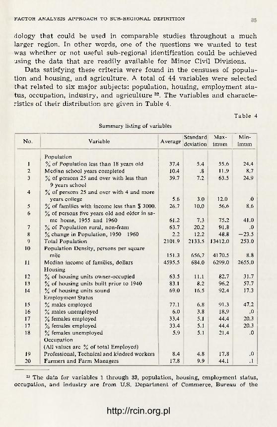
FA.CTOR A N A L Y S I S A P P R O A C H T O S U B - R E G I O N A L D E F I N I T I O N 87
dology that could be used in comparable studies throughout a much larger region. In other words, one of the questions we wanted to test was whether or not useful sub-regional identification could be achieved using the data that are readily available for Minor Civil Divisions.
Data satisfying these criteria were found in the censuses of popula-tion and housing, and agriculture. A total of 44 variables were selected that related to six major subjects: population, housing, employment sta-tus, occupation, industry, and agriculture 32. The variables and characte-ristics of their distribution are given in Table 4.
Table 4 Summary listing of variables
No. Variable Average Standard deviation
Max-imum
Min-imum
Population 1 % of Population less than 18 years old 37.4 5.4 55.6 24.4 2 Median school years completed 10.4 .8 11.9 8.7 3 % of persons 25 and over with less than 39.7 7.2 63.5 24.9
9 years school 4 % of persons 25 and over with 4 and more
years college 5.6 3.0 12.0 .0 5 % of families with income less than $ 3000. 26.7 10.0 56.6 8.6 6 % of persons five years old and older in sa-
me home, 1955 and 1960 61.2 7.3 75.2 41.0 7 % of Population rural, non-fram 63.7 20.2 91.8 .0 8 % change in Population, 1950-1960 2.2 12.2 48.8 -23 .5 9 Total Population 2101.9 2133.5 13412.0 253.0
10 Population Density, persons per square mile 151.3 656.7 4170.5 8.8
11 Median income of families, dollars 4595.5 684.0 6299.0 2655.0 Housing
12 % of housing units owner-occupied 63.5 11.1 82.7 31.7 13 % of housing units built prior to 1940 83.1 8.2 96.2 57.7 14 % of housing units sound 69.0 16.5 92.4 17.3
Employment Status 15 % males employed 77.1 6.8 91.3 47.2 16 % males unemployed 6.0 3.8 18.9 .0 17 % females employed 33.4 5.1 44.4 20.3 17 % females employed 33.4 5.1 44.4 20.3 18 % females unemployed 5.9 5.1 21.4 .0
Occupation (All values are % of total Employed)
19 Professional, Technical and kindred workers 8.4 4.8 17.8 .0 20 Farmers and Farm Managers 17.8 9.9 44.1 .1
33 The data for variables 1 through 33, population, housing, employment status, occupation, and industry are from U.S. Department of Commerce, Bureau of the
http://rcin.org.pl
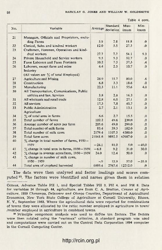
86 B A R C L A Y G . J O N E S A N D W I L L I A M W . G O L D S M I T H
Table 4 cont.
No. Variable Average Standard deviation
Max-imum
Min-imum
21 Managers, Officials and Proprietors, exclu-ding Farms 5.9 2.8 11.8 .0
22 Clerical, Sales and kindred workers 12.0 5.5 27.3 .0 23 Craftsmen, Foremen, Operatives and kind-
dred workers 27.7 7.7 54.1 9.3 24 Private Household and Service workers 9.5 5.3 32.7 .0 25 Farm Laborers and Farm Foremen 10.2 7.3 37.3 .4 26 Laborers, except farm and mine 4.4 2.3 10.7 .0
Industry (All values are % of total Employed)
27 Agriculture and Mining 28.9 15.7 80.0 .6 28 Construction 6.8 3.3 18.6 .0 29 Manufacturing 22.3 11.1 55.6 4.0 30 All Transportation, Comunications, Public
utilities and San. Services 3.8 2.8 16.3 .0 31 All wholesale and retail trade 12.8 6.0 27.1 .0 32 All services 17.3 7.8 40.7 .0 33 Public Administration 2.7 2.1 13.1 .0
Agriculture 34 % of total area in farms 6.6 2.7 15.5 .0 35 Total number of farms 102.2 49.6 230.0 .0 36 Average number of acres per farm 205.6 49.8 299.0 .0 37 Total number of milk farms 83.4 39.3 182.0 .0 38 Total number of milk cows 2179.4 1107.3 4380.0 .0 39 Total farm acres 21141.6 9892.5 43987.0 .0 40 % change in total number of farms, 1950 —
1959 -24.1 11.0 5.0 - 40 .0 41 % change in total area in farms, 1950 — 1959 - 6 . 8 9.2 31.0 30.0 42 % change in average acres/farm, 1950 — 1959 24.0 12.4 50.0 .0 43 % change in number of milk cows,
1950-1959 - .9 15.9 57.0 - 35 .0 44 Total area of cropland harvested 6105.4 2767.4 12212.0 .0
The data were then analyzed and factor loadings and scores com-puted 33. The factors were identified and names given them in relation
Census, Advance Table PH 1, and Special Tables PH 3, PH 4. and PH 8. Data for variables 34 through 44, agriculture, are from C. A. Bratton, Census of Agri-culture, 1959 Chenango, Delaware and Otsego Counties, Department of Agricultural Economics, New York State College of Agriculture at Cornell University, Ithaca, N. Y., September 1962. Where the agricultural data were reported for combinations of towns they were allocated by the ratio: number employed in agriculture in town/ /number employed in agriculture in combined towns.
33 Principle component analysis was used to define ten factors. The factors were then rotated using the "varimax" criterion. A standard program was used and computations were carried out on the Control Data Corporation 1604 computer in the Cornell Computing Center.
http://rcin.org.pl
FA.CTOR A N A L Y S I S A P P R O A C H T O S U B - R E G I O N A L D E F I N I T I O N 87
to the variables that made the greatest contributions. Each of the factors was graphically plotted against all of the others and scatter diagrams scrutinized. Rarely did factor scores cluster noticeably, and division into groups on the ranges of scores did not follow obvious patterns. Conse-quently, factor scores were dichotomized by assigning those above mean value to "high" and those below the mean value to " low". Scores were subsequently dichotomized on two other measures: the median and the mid-range value. In neither case was the arrangement of groups of obser-ved values superior to the original high and low scores arrived at using the mean. Trichotomization was considered, but was of little value for interpretation since it would result in such finely graded groups 34.
Finnally, the five major of the ten derived factors were chosen, the scores for the towns rated high or low, and groupings of similar towns identified.
SUB-REGIONS IN THE THREE-COUNTY AREA
THE FACTORS
In order to discuss the subregions which emerge from the analysis it is first necessary to investigate variables and their relationships and the derived factors that become the indices for classification. The 44 varia-bles were summarized in Table 4 above.
Their intercorrelations are listed below in Table 5, and their values for all Minor Civil Divisions appear in Appendix I. From the most cur-sory examination of Table 5 it is apparent that there are very few high correlations. In fact, out of the total of 946 correlations, only 23 (slightly over 2.4°/o) have correlations greater than. 70, while only 79 or slightly greater than 8.3% have correlations greater than 50.
The highest intercorrelations are within the agricultural category. Most of the other high correlations are between variables in the occupa-tional and industrial categories. Both these phenomena are, of course, to be expected; it is likely, for example, that the percentage of craftsmen, foreman, operatives and kindred workers (Variable 23) would be highly correlated with the percentage of persons employed in manufacturing (Variable 29) and transportation, communications, public utilities and
;;4 Consider for example, four factors. Let towns be combined so that those in similar groups on all factors are together. The groups will be HHHH, HHHL, HHLH, . . . , HHHM, HHMH, . . . ; the total number of possible cominations is 34 = 8)1;. For five factors it is 35, or 243. Recall that the number of towns (and cities) is only 66. For dichotomization the number of combinations drops conside-rably. For four factors it is 24, or 16; for five, 25, or 32.
http://rcin.org.pl

88 B A R C L A Y G . J O N E S A N D W I L L I A M W . G O L D S M I T H
sanitary services (variable 30). It is also expected, for another example, because dairy is the major agricultural activity, that the total number of milk cows per town (Variable 38) will be highly correlated with the total acres farming per town (Variable 39).
The first category of variables, Population, describes several general attributes of the population. Variable 1, the per cent of the population les than 18 years old, tells not only what proportion of the population may be young and dependent, but more importantly, makes suggestions about style of living (rural or urban) and about the future population. Variables 2, 3, and 4 describe the general educational level of the popula-tion, indicating, among other things, past opportunities and present skills. As might be expected, variables 2 and 3 are very highly, and 2 and 4 and 3 and 4 moderately highly, correlated. The last of these, indicating persons with 4 or more years of college, is also highly correlated with the per cent of total employed that are in professional, technical, and kindred occupations (Variable 19). In addition, the college variable is moderately highly correlated with 7 others: positively with total popula-tion (9), median income (11), per cent of total employed who are in clerical, sales and kindred occupations (22), in wholesale and retail trade (31), and in services (32); it is negatively correlated with the per cent employed as farmers and form managers (20) and with the per cent employed in the agricultural and mining industries.
Variables 5 and 11, per cent of families with income less than $ 3000, and median income of families, indicate the present economic level of the population as well as the pattern of income distribution. In addition, to the fact that these two variables are moderately highly correlated, the low income variable (5) is moderately highly correlated with the per cent of persons with less than 9 years school (3). Median income is mo-derately highly correlated with several variables: positively with per cent with college education (4), total Population (9), clerical, sales and kindred workers (22), and per cent employed in manufacturing (29); it is negatively correlated with the per cent of farmers and farm managers (20), and farm laborers and farm foremen (25), with per cent employed in agriculture and mining (27), and with the average number of acres per farm (36). Variable 6, the per cent of persons five years old and older in the same home in 1955 and 1960, is intended to indicate relative mobility, but is such a crude measurement that its implications are questionable.
Variables 7, 8, 9, and 10, per cent of population rural non-farm, per cent change in population 1950—1960, total population, and population density, are self-explanatory. Their correlations with other variables are mentioned when discussing them.
http://rcin.org.pl
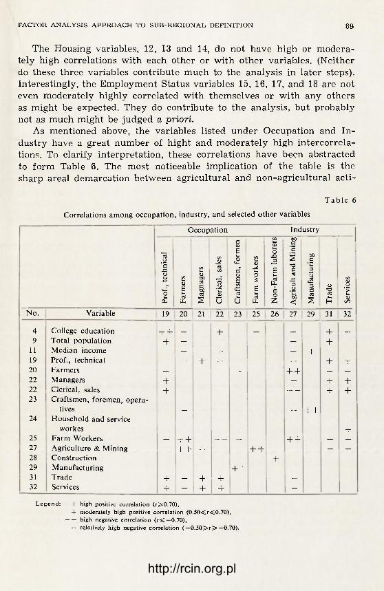
F A . C T O R A N A L Y S I S A P P R O A C H T O S U B - R E G I O N A L D E F I N I T I O N 8 9
The Housing variables, 12, 13 and 14, do not have high or modera-tely high correlations with each other or with other variables. (Neither do these three variables contribute much to the analysis in later steps). Interestingly, the Employment Status variables 15, 16, 17, and 18 are not even moderately highly correlated with themselves or with any others as might be expected. They do contribute to the analysis, but probably not as much might be judged a priori.
As mentioned above, the variables listed under Occupation and In-dustry have a great number of hight and moderately high intercorrela-tions. To clarify interpretation, these correlations have been abstracted to form Table 6. The most noticeable implication of the table is the sharp areal demarcation between agricultural and non-agricultural acti-
Table 6
Correlations among occupation, industry, and selected other variables
Occupation Industry
Prof
., te
chni
cal
Farm
ers
Mag
nage
rs
Cler
ical
, sa
les
Craf
tsm
en, f
orm
en
Farm
wor
kers
Non
-Far
m la
bore
rs
Agri
cult
and
Min
ing
Man
ufac
turi
ng
Trad
e
Serv
ices
No. Variable 19 20 21 22 23 25 26 27 29 31 32
4 College education + + + + + 9 Total population + — — +
11 Median income — + — + 19 Prof., technical — + + — + + 20 Farmers — — — + + — —
22 Managers + — + + 22 Clerical, sales + — + + 23 Craftsmen, foremen, opera-
tives — — + + 24 Household and service
workes + 25 Farm Workers — + + — + + — —
27 Agriculture & Mining — + + — — + + — —
28 Construction + 29 Manufacturing + + 31 Trade + — + + —
32 Services + - + + -
L e g e n d : + + high positive correlation ( r > 0 . 7 0 ) , + moderately high positive correlation ( 0 . 5 0 < r < 0 . 7 0 ) ,
high negative correlation ( r < — 0 . 7 0 ) , — relatively high negative correlation ( — 0 . 5 0 ^ r > —0.70).
http://rcin.org.pl
90 B A R C L A Y G . J O N E S A N D W I L L I A M W . G O L D S M I T H
vities. At all intersections of agricultural columns with agricultural rows the correlations are high and positive, and at all other intersections with the agricultural columns and rows the correlations are either low or negative. There do not appear to be any totally unexpected results demonstrated in the table.
The last 11 variables, in the Agricultural category, are more highly intercorrelated than any other of the variable groups. This, of course, is reasonable since nearly all of them measure the relative intensity of agricultural activity. The high positive correlations between all pairs of variables 35, 37, 38, 39 and 44 strongly reinforce the observation that agricultural activity in the region is dominated by the dairy industry. Variable 34 is also moderately highly correlated with each of these vari-ables. The moderately high intercorrelations between variables 40, 41 and 42 suggest that the more a town's total number of farms decreased in the decade 1950—1960, the more the average acreage tended to in-crease, indicating that larger, more efficient farming operations were being undertaken.
With this description of what appear to be the important relations-hips among the variables it is possible to examine the composition of the factors. The five major factors will be discussed. Following the descrip-tion of the factors we will use their scores to interpret various delinea-toins of subregions.
The factors and the variables which contribute most heavily to them are given in Table 7.
For comparative purposes we have listed for each factor the eleven or twelve variables which are most highly correlated with it. For a rea-sonable basis of discussion we assume that a loading smaller in absolute value than 0.075 does not significantly affect the character of the factor.
Factor I, High Index Urban, is inversely related to an aggregation of many variables which indicate level of education, level of occupation, and level of industrial employment. Since the loadings are negative, high values in the varriables give low factor scores. Clearly, the factor is an indicator of an urban way of living.
What does a high negative value on Factor I imply? First, it suggests a high level of education, with high median school years completed, and with a relatively large percentage of the population over 25 that had completed over four years of college. Secondly, it suggests that the po-pulation is employed in the higher occupation groups, as non-farm ma-nagers, officials and proprietors, as professional and technical workers, and as clerical and sales workers. It also suggests a relatively large num-ber of private household and service workers, and few laborers. Fourthly, high negative value on Factor I suggests that a relatively large propor-
http://rcin.org.pl

FA.CTOR A N A L Y S I S A P P R O A C H T O S U B - R E G I O N A L D E F I N I T I O N 9 1
Table 7 Factor Descriptions in rank order of correlations with top quartile variables
Vbl. No. I Loading Description FACTOR I --HIGH INDEX URBAN
2 - .314 Median school years completed. 21 - .239 Managers, officials and proprietors, excluding farms. 30 - .211 All transportation, communications, public utilities and san.
service. 4 - .179 % of persons 25 and over with four and more years of
college. 19 - .149 Professional, technical and kindred workers. 24 - .131 Private household and service workers.
1 .115 % of population less than 18 years old. 21 - .113 All services. 31 - .109 All wholesale and retail trade. 22 - .105 Clerical, sales and kindred workers. 33 - .095 Public administration 26 .088 Laborers, except farm and mine.
FACTOR II - H I G H INDEX AGRICULTURE
2 .245 Median school years completed. 34 .241 % of total area in farms. 16 - .056 % males unemployed. 21 .048 Managers, officials and proprietors, excluding farms. 19 .042 Professional, Technical and kindred workers. 26 - .038 Laborers, except farm and mine. 15 .037 % males employed. 3 .034 % of persons 25 and over with less than 9 years scholl.
33 - .033 Public administration. 6 .028 % of persons five years old and older in same home, 1955
and 1960. 18 - .027 % females unemployed.
FACTOR III —MIDDLE INDEX URBAN
23 .119 Craftsmen, foremen, operatives and kindred workers. 25 - .081 Farm laborers and farm foremen. 29 .079 Manufacturing. 22 .079 Clerical, sales and kindred workers.
6 - .067 % of persons five years old and older in some home, 1955 and 1960.
20 - .056 Farmers and farm managers. 4 .050 % of persons 25 and over with four and more years college.
17 .047 % females employed. 1 .045 % of population less than 18 years old.
12 .044 % of housing units owner-occupied. 19 .043 Professional, technical and kindred workers.
http://rcin.org.pl

92 B A R C L A Y G . J O N E S A N D W I L L I A M W . G O L D S M I T H
Table 7 cont.
FACTOR IV —LOW INDEX URBAN
2 - . 272 Median school years completed. 33 .254 Public administration. 16 .122 % males unemployed. 34 - . 097 % of total area in farms. 41 - .074 % change in total area of farms, 1950 — 1959. 4 - 060 % of persons 25 and over with four and more years college.
17 - .051 % females employed. 1 .049 % of population less than 18 years old.
21 .049 Managers, officials and proprietors, excluding farms. 28 .049 Construction. 43 - . 045 % change in number of milk cows, 1950 — 1959.
FACTOR V - LOW INDEX AGRICULTURE
2 - .219 Median school years completed. 30 - .109 All transportation, communications, public utilities and san.
services. 40 - .074 % change in total number of farms, 1950 — 1959. 42 .066 % change in average acres/farm, 1950 — 1959. 21 .064 Managers, officials and proprietors, excluding farms. 16 .048 % males unemployed. 34 .046 % of total area in farms. 17 .045 % females employed. 31 - .029 All wholesale and retail trade. 26 .028 Laborers, except farm and mine. 4 - .025 % of persons 25 and over with four and more years college.
tion of occupants are employed in public utilities, in service industries, in wholesale and retail trade, and in public administration. Lastly, the positive loading on Variable 1 suggests a relatively small proportion of children. The combination of all these variables very strongly indicates that Factor I is an index of urbanization, and an index of quite high--status urban living in addition.
Factor II, High Index Agriculture, appears, quite simply, to indicate towns in which there is a high percentage of land in farms and in which the population is relatively well educated. The loadings on variables other than 2 and 34 are so low that the contributions of the former are only slightly more than negligible. The factor, therefore, appears to be an index of agricultural areas with well educated populations. Whether those in the areas who are well educated are the farmers or others is
http://rcin.org.pl

FA.CTOR A N A L Y S I S A P P R O A C H T O S U B - R E G I O N A L D E F I N I T I O N 9 3
not explained sufficiently by the factor; we will later analyze this con-sideration in light of other information.
Factor III, Middle Index Urban, is constituted primarily of occupation and industry variables. A high score on the factor indicates a relatively high percentage of craftsman, foremen, operatives, clerical workers and sales workers. It also indicates a relatively low number of farm workers. In addition, a high score on the factor suggests a relatively high pro-portion of total employment in the manufacturing and craftsman, fore-men, and operatives categories.
These first three factors, High Index Urban, High Index Agriculture, and Middle Index Urban explain a good deal about the population and activities. For the most part, they are positive measures, describing the presence, or absence, of particularly favorable or prosperous Minor Civil Divisions within the three-county region. The construction of the other two factors, IV and V, suggests they are indices of adversity rather than affluence. With the addition of them to the first three factors we may be able to identify areas of both relatively high and low economic standing.
Factor IV, Low Index Urban, is made primarily from four variables. A negative loading on median school years completed means that a high value on the factor suggests a low educational level. The positive lo-adings on public administration and male unemployment suggest for a high factor score relatively high levels of both government employment and unemployment, perhaps indicating a paucity of private employment. Finally, the negative loading on the percentage in farming of the total area means that a high score indicates a town with less farming activity than others.
Factor V, Low Index Agriculture, really has only two variables which contribute significantly. Again, as in Factor IV, a high score suggests a low eductional level. On the other hand, the presence of a negative loading with the public utilities industries suggests a non-urban charac-ter to areas with high scores. Further investigation will tendl to substan-tiate these inferences about the meaning of the factors.
The five factors so far discussed, while being the best indicators of subregional definition we were able to derive, do not by any means explain all the variation of the original variables. The first three factors, the indices of relative affluence, account for about 40% of the original variation. The next two, the adversity indices, account for about 10°/o more variation. The addition of five more factors (which have not been used for analysis) contributes an explanation for about 25% more of the variation. The relevant information is presented in Table 8.
http://rcin.org.pl
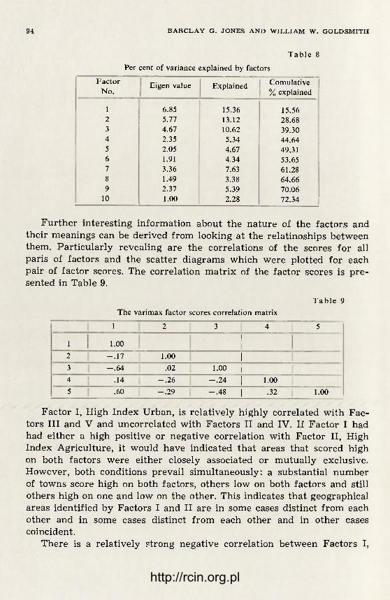
9 4 B A R C L A Y G . J O N E S A N D W I L L I A M W . G O L D S M I T H
Table 8 Per cent of variance explained by factors
Factor No.
Eigen value Explained Comulative % explained
1 6.85 15.36 15.56 2 5.77 13.12 28.68 3 4.67 10.62 39.30 4 2.35 5.34 44.64 5 2.05 4.67 49.31 6 1.91 4.34 53.65 7 3.36 7.63 61.28 8 1.49 3.38 64.66 9 2.37 5.39 70.06
10 1.00 2.28 72.34
Further interesting information about the nature of the factors and their meanings can be derived from looking at the relatinoships between them. Particularly revealing are the correlations of the scores for all paris of factors and the scatter diagrams which were plotted for each pair of factor scores. The correlation matrix of the factor scores is pre-sented in Table 9.
Table 9 The varimax factor scores correlation matrix
1 2 3 4 5
1 1.00 |
2 - . 1 7 1.00 1 3 - . 6 4 .02 1.00 I 4 .14 - . 2 6 - . 2 4 | 1.00 5 .60 - . 2 9 - . 4 8 | .32 1.00
Factor I, High Index Urban, is relatively highly correlated with Fac-tors III and V and uncorrelated with Factors II and IV. If Factor I had had either a high positive or negative correlation with Factor II, High Index Agriculture, it would have indicated that areas that scored high on both factors were either closely associated or mutually exclusive. However, both conditions prevail simultaneously: a substantial number of towns score high on both factors, others low on both factors and still others high on one and low on the other. This indicates that geographical areas identified by Factors I and II are in some cases distinct from each other and in some cases distinct from each other and in other cases coincident.
There is a relatively strong negative correlation between Factors I,
http://rcin.org.pl
FA.CTOR A N A L Y S I S A P P R O A C H T O S U B - R E G I O N A L D E F I N I T I O N 95
High Index Urban, and III, Middle Index Urban. The scatter diagram shows most of the towns that are low on Factor I are high on Factor II and vice versa. Because these two factors both measure diffe-rent aspects of the same general socio-economic pattern ( and Factor I is inversely related to its constitutent variables) a strong relationship of this kind is to be expected.
The correlation between Factor I, High Index Urban, and Factor IV, Low Index Urban, is very low and the scatter diagram shows no discer-nable pattern. Factor IV is related to relatively low quality non-agri-cultural components, and the relationship between the two factors in-dicates that these components are sometimes present and sometimes absent in areas with high urban indices.
There is a relatively strong positive correlation between Factor I, High Index Urban, and Factor V, Low Index Agriculture. The scatter diagram shows that most of the towns are either high on both factors or low on both. Because Factor V is an index of least successful non--urban activity, this relationship indicates that the most and least suc-cessful components of urban and non-urban activity seldom occur in the same towns.
The correlation coefficient between Factor II, High Index Agricul-ture, and Factor III, Middle Index Urban, is the smallest for any pair of factors. The pattern is similar to that between Factors I and II. The scatter diagram is widely dispersed with relatively equal numbers of towns having scores that are high on both factors, low on both, and high on one and low on the other. These urban and agricultural components are shown to occur separately in some places and to coincide in others.
There is a somewhat stronger correlation between Factor II, High Index Agriculture, and Factor IV, Low Index Urban, than there is bet-ween Factors I and IV. This indicates that there is less tendency for the low index non-agriculture components to occur in high index, successful agricultural areas than there is the high index urban areas.
A similar negative relationship is shown between Factor II, High Index Agriculture, and Factors V, Low Index Agriculture However, re-ference to the scatter diagram indicates a pattern of stronger relation-ship between these two factors than the correlation coefficient suggests. The value of the coefficient is as low as it is because of a few highly deviant observations caused by the cities and other highly urban areas. Disregarding these urban communities, the diagram, indicates, that low index and high index agricultural components seldom coincide.
There is a slight negative relationship shown between Factor III, Middle Index Urban, and Factor IV, Low Index Urban. The correlation coefficient is higher and the pattern of the scatter diagram more pro-
http://rcin.org.pl

96 B A R C L A Y G . J O N E S A N D W I L L I A M W . G O L D S M I T H
nounced than for the relationship between Factor I and IV. This indi-cates a somewhat lesser likelihood that the low index non-agricultural components will be found in areas with middle index urban ones.
There is a somewhat stronger negative relationship between Factor III, Middle Index Urban, and Factor V, Low Index Agriculture. The scatter diagram shows that most of the towns are either high on Fac-tor V and low on Factor III or vice versa. In other words, this middle range of urban components often is found in completely separate areas from least successful agricultural activities. It should also be noticed that the relationship is of the same order, but less strong, and the scatter diagram less pronounced, than for Factors I and V. That is, there is a somewhat higher degree of coincidence of the middle range urban and low index agricultural indices than of the high urban and low agri-cultural indices.
There is a positive relationship between Factors IV, Low Index Urban, and V, Low Index Agriculture. Reference to the scatter diagram, however, indicates no coherent pattern of association. The most that can be said is that there is a group of towns with relatively high scores on both of these low index factors and another group with low scores on both. Most of the towns, however, are rather tightly clustered around the origin.
The factors seem to relate to useful indices of geographical region-alization. They seem to perform in logical and predictable fashion with reference to each other. It seems likely that they identify geographical sub-regions within the study area that are both interesting and infor-mative.
SUB-REGIONAL IDENTIFICATION
As mentioned earlier, once factors are determined, and their scores calculated, discrimination among the units of observation is carried out in the same way as if the discrimination were being made by means of a single variable. That is, once he factor scores are established for each town the scores are used as variable values would be for further ana-lysis. A summary listing of the factor scores appears in Table 10.
Even with the vast simplification resulting from the use of only five factors in place of the original 44 variables the picture is rather con-fusing. Visual scanning of Table 9 does give limited information about the most extreme situations for each factor, but allows little else. Two manipulations of the factor scores can improve our perception. First we will dichotomize the scores on each factor and construct a tree-diagram
http://rcin.org.pl

FA.CTOR A N A L Y S I S A P P R O A C H T O S U B - R E G I O N A L D E F I N I T I O N 97
giving us a set of results which exhausts all contingencies. Next we will examine the extreme values on each factor. In each case we will make inferences about the internal structure of the hree-county region and compare them with other information about the area.
First we wished to group the minor civil divisions of the region into mutually exclusive and exhaustive sets by very crudely dividing them into "high" and " low" on the basis of some dichotomization of the scores for each factor. An arbitrary choice of method was required, for
Table 10 Summary listing of factor scores
No. Factor High Low Mean
I High index urban (negative) 17.9 -21 .6 0 II High index agriculture 12.3 -13 .7 0
III Middle index urban 11.3 -14 .9 0 IV Low index urban 9.1 - 6 . 5 0 v Low index agriculture 4.8 - 9 . 2 0
when the values of any one of the five factors are plotted there are dis-tinct breaking points only near the ends; that is, except for a very few minor civil divisions with extreme factor scores, there is a relatively uniform continuum from the lower to the higher scores for each factor. In the absence of any other information, dichotomization on the mean value appears justified.
The results of dichotomization of the factor scores at the mean value are shown in Fig. 7, the Factor Scores Tree Diagram. The towns and cities are listed by their designations according to Table 4 in Chapter II. For Factor I, a low score meaning the existence of High Index Urban elements is indicated by the first right hand branch; for Factor II, high scores meaning the existence of High Index Agricultural elements are indicated by the second right hand branch, whether coming from the right or left of the original split on Factor I. For Factor III high scores on the right show the presence of Middle Index Urban elements. And for Factors IV and V, high scores for these Low Index Urban and Agriculture factors are again on the right.
Let us take an example. Consider Minor Civil Division 7, Guilford Town in Chenango County. Its scores on factors one through five are the following, in order: 2.82, 5.90, 2.76, 0.22, and — 0.59 Because the mean score for each factor is zero, the first four scores for Guilford Town are "high" and the last, on Factor V, is " low". Tracing these scores down the tree diagram we do the following: For Factor I we go to the left for the high score until we come to the next branch in the tree; we then
7 G e o g r a p h i a Polonica t. 15
http://rcin.org.pl
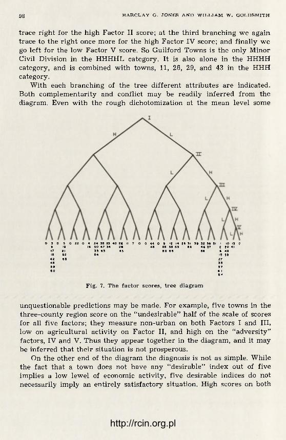
98 B A R C L A Y G . J O N E S A N D W I L L I A M W . G O L D S M I T H
trace right for the high Factor II score; at the third branching we again trace to the right once more for the high Factor IV score; and finally we go left for the low Factor V score. So Guilford Towns is the only Minor Civil Division in the HHHHL category. It is also alone in the HHHH category, and is combined with towns, 11, 26, 29, and 43 in the HHH category.
With each branching of the tree different attributes are indicated. Both complementarity and conflict may be readily inferred from the diagram. Even with the rough dichotomization at the mean level some
O 3 0 S O 22 O 4 24 38 23 40 26 II 7 0 O 44 O 9 12 14 28 31 39 32 36 81 I 10 13 0 8 19 16 30 47 34 2« 48 28 38 83 82 46 37 2 20 41 17 21 33 63 43 80 86 66 6 49 18 62 84 IS 88 42 65 27 48 38 8» S 7 • 0 a I 6*
Fig. 7. The factor scores, tree diagram
unquestionable predictions may be made. For example, five towns in the three-county region score on the "undesirable" half of the scale of scores for all five factors; they measure non-urban on both Factors I and III, low on agricultural activity on Factor II, and high on the "adversity" factors, IV and V. Thus they appear together in the diagram, and it may be inferred that their situation is not prosperous.
On the other end of the diagram the diagnosis is not as simple. While the fact that a town does not have any "desirable" index out of five implies a low lewel of economic activity, five desirable indices do not necessarily imply an entirely satisfactory situation. High scores on both
http://rcin.org.pl
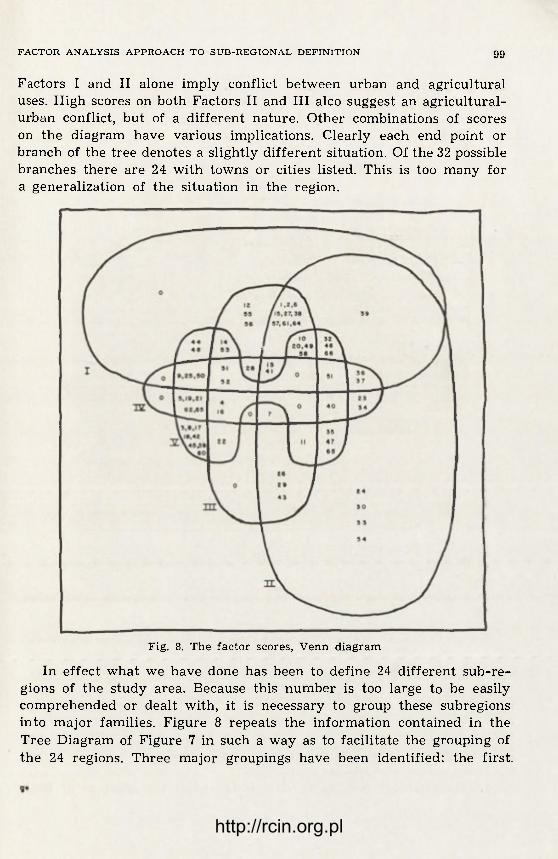
FA.CTOR A N A L Y S I S A P P R O A C H T O S U B - R E G I O N A L D E F I N I T I O N 9 9
Factors I and II alone imply conflict between urban and agricultural uses. High scores on both Factors II and III alco suggest an agricultural-urban conflict, but of a different nature. Other combinations of scores on the diagram have various implications. Clearly each end point or branch of the tree denotes a slightly different situation. Of the 32 possible branches there are 24 with towns or cities listed. This is too many for a generalization of the situation in the region.
Fig. 8. The factor scores, Venn diagram
In effect what we have done has been to define 24 different sub-re-gions of the study area. Because this number is too large to be easily comprehended or dealt with, it is necessary to group these subregions into major families. Figure 8 repeats the information contained in the Tree Diagram of Figure 7 in such a way as to facilitate the grouping of the 24 regions. Three major groupings have been identified: the first.
http://rcin.org.pl

1 0 0 B A R C L A Y G . J O N E S A N D W I L L I A M W . G O L D S M I T H
includes all those regions with High Index Urban elements; the second includes all those regions with High Index Agricultural elements except those in the first grouping; and the third includes all those regions out-side the first two groupings that have Low Index Agricultural elements.
Fig. 9. Regions with high index agricultural and high and middle index urban elements
We will examine each of these groupings in detail. The discussion will refer also to Figs 9 and 10, on which are mapped the presence and ab-sence of Index elements.
Grouping I (all High Index Urban regions): The High Index Urban regions can be divided into two groups, one
with High Index Agricultural elements and one without. The former defines areas of conflict within the three-county study region.
Areas of conflict are discussed first: 1. The first category of conflict is identified by presence of both
http://rcin.org.pl

FA.CTOR A N A L Y S I S A P P R O A C H T O S U B - R E G I O N A L D E F I N I T I O N 1 0 1
High Index Urban and Agricultural elements (I and II) and no other elements. Only one town falls into this category: Stamford, (39). A glance at both Figs. 9 and 10 shows Stamford as the only town with these and only these two elements. As indicated in Fig. 9, its agricultural elements
Fig. 10. Regions with absence of all high and middle index elements and presence of low index urban and agricultural elements
are contiguous with a suburban and rural non-farm area stretching from Worcester to Delhi and Middletown. The absence of Low Index elements in Stamford is indicated on Fig. 10.
2. The second category of conflict, the highest order conflict, is identified by presence of both High and Middle Index Urban elements and High Index Agricultural elements. Here are Balanced Urban areas in conflict with agriculture. Three cases exist.
http://rcin.org.pl
102 B A R C L A Y G . J O N E S A N D W I L L I A M W . G O L D S M I T H
a) In the first, with Factors I, II and III alone, there are 9 towns: Afton (1), Bainbridge (2), Greene (6), Oxford (15), Delhi (27), Sidney (38), Otego (57), Richfield (61), and Unadilla (64). Figure 9 shows that, except for Delhi and Richfield, these towns are contiguous and grouped rather tightly around the juncture of the three counties, at the village of Sidney in the Susquehanna Valley. These are the strongest urban areas which are in conflict with important agricultural uses. (Other towns are indicated identically on Fig. 9, but Fig. 10 shows the presence of Low Index elements for them). It is of particular interest to compare the belt of five towns from Afton to Otego, along Route 7, and the Chenango--Tioga soil bed in the same area shown in Figure 4. These towns, with the addition of several others on longer in conflict with agricultural uses, define the major urban focus of the three-county region.
b) The second case within this second category of conflict is iden-tified by the additional presence of Low Index Urban elements, i. e., by the presence of I, II, III and IV. Two towns, Norwich (13) and Walton (41), provide instances of this kind of Complete Urban area in conflict with agricultural uses. The interpretation of the Balanced Urban areas in conflict is reinforced. Here we see that Norwhich extends the line through Greene and Oxford along Route 12 nad another Chenango-Tioga soil bed. So with the addition belew of non-conflicting urban areas, the minor focus of urban activity within the three-county region will be identified along this valley.
c) The third case within the second category of conflict is identified by the presence, in addition to elements I, II and III, of Low Index Agri-cultural elements (V). There are four such towns, New Berlin (10), Sherburne (20), Laurens (49), and Otsego (58). With the addition of this group the minor urban axis through Chenango County is extended to the border at Sherburne, and a branch is added to the major urban axis with Laurens ond Otsego (Hartwick, between them, is part of the branch, but without the agricultural conflict).
3. The third category of conflict is identified by the presence of High Index Urban and Agricultural elements plus combinations of Low Index Urban and Agricultural elements. Since they lack Middle Index Urban elements, the conflict in these towns is of lesser magnitude. Three cases exist here also.
a) In the first case, with Low Index Urban (i. e., I, II and IV only), there are only two towns, Middletown (36) and Roxbury (37). These towns are clearly out of the areas of major urban activity within the study area. Their urban quality is lower than the towns mentioned above.
b) In the second case, where elements of I, II and V appear, there are three towns, Harpersfield (32), Edmeston (46), and Worcester (66).
http://rcin.org.pl

FA.CTOR A N A L Y S I S A P P R O A C H T O S U B - R E G I O N A L D E F I N I T I O N 103
Harpersfield and Worcester are in the suburban area mentioned above in the discussion of Stamford Town. They differ from Stamford in that all three of these towns have Low Index Agricultural components as well as High Index ones in conflict with urban uses.
c) In the third and final case, where elements of I, II, IV and V all appear, there is only one town, Middlefield (51). Here there are both high and low urban and high and low agricultural uses in conflict with each other. This town contains a part of Cooperstown as well as some tiny remote villages. It has a fine agricultural valley and many inacces-sible and unfertile areas.
One of the striking features of the areas of conflict within the region is their contiguity. There seem to be several complementary explanations for this phenomenon. First, because agricultural regions depend upon soils and topography, they tend to be limited to relatively compact sec-tors chiefly along the valleys. Secondly, urban and suburban populations are effectively held close to the major urban regions by the time and cost of travel. Thirdly, in this historical pattern of development, the urban centers, which were first established to serve surrounding agri-cultural areas, have developed into the major urban uses and tend to coincide with the major agricultural activities. Finally, transport routes generating urban uses have similar topographical requirements as agri-culture. There are, of course, other forces working within the study area, but those mentioned seem to explain a large part of what we have so far examined.
There are also balanced and complete urban areas without conflict: 1. In the first category of this non-conflict group are only three towns:
Norwich City (12), Oneonta City (55), and Oneonta Town (56). They each contain only High and Middle Index Urban elements. They are clearly the most urban Minor Civil Divisions within the three-county region, and they lie at the centers of the major urban areas. It can also be seen, by referring to Figs. 1 and 4, that these communities lie on both the best soil areas and on the two major routes through the region. The absence of agricultural conflict can be explained by the urban uses having crowded out agriculture at some previous point.
2. In the second category within this non-conflict group there are three cases, one with Low Index Urban elements. The fact that Route 17, a major New York highway, lies inside its borders undoubtedly explains the presence of this complete range of urban activities.
In the second case there are two towns, Hancock (31) and Milford (52). Both have Complete Urban components with Low Agricultural ones.
In the third case there are also two towns, Otselic (14), and Morris (53). They have Balanced Urban components with Low Agricultural ones.
http://rcin.org.pl

1 0 4 B A R C L A Y G . J O N E S A N D W I L L I A M W . G O L D S M I T H
Because of their locations, and their components, each of the four towns in these last two cases can be classified as primarily sub-urban and rural non-farm, but with concentrations in old villages. That is, a large part of the employment of the residents of these four towns probably exists in other towns, but concentrated settlements still exist in the former towns. •
Other urban areas without conflict can be seen: 1. Two more groups with High Index Urban elements remain. The
first, with three towns, has, in addition to elements of I, both Low Index Agricultural and Urban elements. The towns are McDonough (9), Col-chester (25), and Maryland (50). Each of these towns can be identified on Fig. 9 by the presence of only High Index Urban elements, and on Fig. 10 by the presence of both low elements. There is a relatively high precentage of rural non-farm occupants in these three towns (see Ap-pendix) which probably explains the presence of the high urban ele-ments.
2. There are two towns in the second case that have both High Index Urban and Low Index Agricultural elements: Cherry Valley (44) and Hartwick (48). Again, each of these towns has a relatively high percen-tage of residents classed as rural non-farm indicating a relatively large commuting population living in the same areas with less successful agricultural populations. This completes discussion of Grouping I, those regions with High Index Urban Components. New we want to consider Grouping II, which includes all those regions not already discussed which have High Index Agricultural Components.
Grouping II (High Index Agricultural without High Index Urban):
Within this grouping there are two categories. The first, which con-tains Middle Index Urban components, is in minor conflict, and the second, which contains only Low Index elements in addition to the High Agricultural elements, is not in conflict.
Areas of minor conflict are discussed first: These areas, with both High Index Agricultural and Middle Index
Urban elements, fall into three classes. 1. In the first, which is comprised of Davenport (26), Franklin (29)
and Butternuts (43), there are High Index Agricultural and Middle Index Urban components. These three towns are on the periphery of the major urban area of the region but have found it possible to maintain their agricultural uses. It is very likely that large portions of the non-farm dwellers in these three towns live in villages. Smaller proportions are rural, non-farm, and suburban.
2. The second category is comprised of a town that also has Low
http://rcin.org.pl

FA.CTOR A N A L Y S I S A P P R O A C H T O S U B - R E G I O N A L D E F I N I T I O N 105
Index Urban elements. This town, Guilford (7), has middle and low urban and high agricultural components.
3. The third category, which also has only one town, North Norwich (11), has high and low agricultural elements and middle urban elements. The towns in both of the last two classes lie just off the minor urban axis through Norwich City, and both probably accommodate a good portion of the working population of Norwich, as well as maintaining agricultural land.
There are also areas without conflict: Within this last agricultural category lie four classes. 1. In the first, where the only elements found are High Index
Agricultural, there are four towns: Bovina (24), Hamden (30), Kortright (33) and New Lisbon (54). Each of these towns has productive agricultural land and is accessible from major transport routes but is not in the path of major urban uses. Much of the other area of the best agricultural land lies under the cities and suburban areas and it will never return to agri-cultural use. These towns are important in that they are still in agricul-ture, and account for substantial agricultural production. They should probably be regarded in that light in future planning.
2. The second class of agricultural region not in conflict with urban uses is composed of two towns, Andes (23) and Masonville (34). The dif-ference between this and the previous class is that these two towns contain Low Index elements. Again, these elements are most likely si-tuated in villages in the towns, allowing the use of the land for agri-cultural production.
3. The third category, with only one town, Tompkins (40), has, in addition to High Agricultural and Low Urban, Low Agricultural ele-ments. This situation has probably deteriorated since the reservoir went in.
4. Finally, three towns, Meredith (35), Exeter (47) and Springfield (63), have only High and Low Index Agricultural elements. These towns, a little out of the commuting pattern, have both viable and unprofitable farms, probably differentiated primarily by topography.
Grouping III (the remaining Low Index Agricultural areas): Within this grouping there are two quite distinct categories. In the
first there are elements of Middle Index Urban, and in the second there are no High or Middle Index elements, suggesting that this category includes the least advantaged towns in the three-county region.
In the first category there are two cases: 1. The first, containing only Smyrna (22), has only Middle Index
Urban and Low Index Agricultural elements. Reference to Figure 9 in-
http://rcin.org.pl

106 B A R C L A Y G . J O N E S A N D W I L L I A M W . G O L D S M I T H
dicates that the urban components are contiguous with an extensive region covering a number of towns of norther Chenango County. Figure 10 indicates a similar situation with respect to the low agricultural ele-ments, although in this case the region is more extensive.
2. In the second case there are two towns, Coventry (4) and Phar-salia (16). These towns have, in addition, Low Index Urban elements. Pharsalia can be seen on Figs. 9 and 10 to be in the same regions men-tioned above for Smyrna, and, in addition, to be in a Low Index Agri-cultural region in the western part of Chenango County. Coventry lies between the two major valleys.
In the second category there are also two cases: 1. In the first case only Low Index Agricultural elements are present.
Towns in this case are Columbus (3), Lincklaen (8), Pitcher (17), Ply-mouth (18), Burlington (42), Decatur (45), Pittsfield (59) and Plainfield (60).
2. In the second case there are five towns: German (5), Preston (19), Smithville (21), Roseboom (62) and Westford (64). In these two sets of towns there are elements of both Low Index Agriculture and Low Index Urban. Both these cases are depicted in Fig. 10. These two cases re-present the more disadvantaged regions. In one case only Low Index Agricultural elements register, and in the other there are both Low Index Agriculture and in the other there are both Low Index Agriculture and Urban components.
The entire second category of Grouping III, the 13 towns without any High or Middle Index elements, is represented in Fig. 10 by the dot-ted areas. They can be seen to be tightly clustered in two areas, western Chenango and eastern Otsego, and loosely in northern Chenango and Otsego. Through a combination of their distance from the urban centers, poor soils, rugged topography, and poor accessibility, these towns are among the least viable economic areas in the study region.
As a final part of the analysis, one additional manipulation of the factor scores for the towns of the region has been made. By visual scan-ning of the scatter diagrams of the factor scores (scores were actually scanned along only one axis at a time) extreme values and the Minor Civil Divisions associated with them were picked out for each factor. The towns are marked on the map in Fig. 11. It is expected that the towns chossen should best represent the extreme cases in the region, and thus illustrate more clearly areas of prospective growth and decline. In addition, because there was little overlap interpretation is quite simple.
For Factor I, High Index Urban, five Minor Civil Divisions are clearly at the extreme negative end of the scale. Three, Oneonta City, Oneonta Town, a nd Norwich City, are, without a doubt, the most urban com-
http://rcin.org.pl

FA.CTOR A N A L Y S I S A P P R O A C H T O S U B - R E G I O N A L D E F I N I T I O N 107
munities of the three-county region. The two additional towns, Richfield and Otsego, are special cases. Richfield is located on Route 22 and in addition is close to Utica, to which large numbers of workers commute. Otsego contains Cooperstown, a very special kind of urban place, and has the largest resort activity in the three-county region. It is the county seat and contains state and national institutions which give it a different and more urban character.
Factor II, High Index Agriculture, has extremely high values for five towns: Greene, Bainbridge, Franklin, Walton, and Delhi. Portions of each of these towns contain the excellent soils of the Chenango-Tioga Asso-ciation (see Fig. 4). Also, each of them except Bainbridge is presently far enough away from the major urban areas of Oneonta, Norwich, and Sidney to remain in agricultural use. These towns have productive agri-
http://rcin.org.pl
110 B A R C L A Y G . J O N E S A N D W I L L I A M W . G O L D S M I T H
cultural land that is being used for production, and this is why they rank highly on Factor II.
For Factor III, Middle Index Urban, there are six Minor Civil Divi-sions with extremely high values. They are the two cities and the Towns of Oneonta, Norwich, Unadilla, Sidney and Bainbridge. These extremes are expected a priori in the cities and their towns, and should be ex-pected in the other three as well because of the large employment con-centration at Sidney. These very tightly clustered areas in which large numbers of manufacturing workers live shows that there is some ten-dency to agglomerate around employment centers.
Factor IV, Low Index Urban, has extreme values for nine towns. They are shown in three distinct regions on the map. In Chenango there are German, McDonough, and Smithville; in Delaware are Tompkins, Hancock, Colchester, Andes, and Middletown; and in Otsego is Roseboom. Only three of these towns, all in Delaware, have High Index Agricultural elements present also: Middletown, Andes, and Tompkins (see Fig. 9). So, except for these three towns, the extreme values on Factor IV probably represent past agricultural land which is no longer competitive, from which the population has migrated, and to which no major new employ-ment opportunities have come. Clearly these regions, including the three towns with High Index Agricultural elements, are also areas of least advantaged populations.
One of the interesting properties of factor analysis is that study of the results continues to yield insights concerning the sub-areas for a long period of time. Alternative presentations of the findings and other methods of discussing them could be given, but they would only serve to reinforce the material already presented.
CONCLUSIONS
Factor analysis has been shown to be a useful tool for rapidly sur-veying a region to identify and define meaningful sub-regions. When combined with other methods of analysis, other information, and some familiarity with the study area it can provide extremely useful insights about the nature of sub-areas. It is useful in two ways. First, it divides the region into more manageable homogeneous sub-regions as a focus for further study. Second, it is very helpful in looking in greater detail at individual areas or Minor Civil Divisions. Similarities and differences between the town in question and others in the region help to identify its characteristics and lead to better understanding of it.
Perhaps no new information or understanding is gained by factor
http://rcin.org.pl

FA.CTOR A N A L Y S I S A P P R O A C H T O S U B - R E G I O N A L D E F I N I T I O N 1 0 9
analysis that cannot be attained by other methods. That is beside the point. The relevant question is whether or not factor analysis is a more efficient method than the others for an initial investigation of an exten-sive and complex region. We feel that findings presented above indicate that it is very successful in this respect.
One of the purposes of this study was to explore various methods. Other means of analysis were used also. The results of these methods have been compared to the factor analysis findings throughout the pre-vious discussion and the results themselves made available in the com-panion report cited earlier. For the most part the results of the various methods confirm each other. To some extent there are differences. In some cases the differences are more apparent than real. The messages may not be contradictory but the interpretations that have been made from them may be in conflict. In such cases the use of a number of methods leads to deeper insights into the complexity of the system. In other situations the divergent findings may be quite real. The source may be the data; measurement error, sampling error, irrelevancy. Or the source may be statistical "noise" resulting from the particular method selected. In such cases there will be errors and care must be exercised in the use of the findings.
Factor analysis in shown to be a useful device for initial scrutiny of sub-regionalization in underdeveloped regions with some qualifications. First, more experimentation with the original variables than was pos-sible in this study might prove helpful. Trials should be made discarding some variables and adding others. Various transformations of the varia-bles should be tried. Linear relationships were assumed for all variables in this study. Root and logarithmic transformations should be attempted to achieve better fits. Many of the variables used here were standardized into percentage terms. Trials should be made using the raw data. Other data were used in raw form and consideration should be given to trans-forming them. Experimentation of this kind might make factor analysis an even more useful tool.
The factor analysis indicated that the three-county region contained three relatively homogeneous sub-regions. In the first of these, urban life patterns were predominant although there were no major urban areas. This sub-region accounted for 35 of the 66 Minor Civil Divisions or 53°/o. The second sub-region was identified as one containing strong agricultural components. It accounted for 37 of the 66 Minor Civil Divi-sions or 56°/o. The first two regions overlapped. A total of 22 Minor Civil Divisions were common to both regions. The intersect of these re-gions defined an area in which urban and agricultural uses were in con-flict which was larger than any of the other defined regions. Only 13 of
http://rcin.org.pl

110 B A R C L A Y G . J O N E S A N D W I L L I A M W . G O L D S M I T H
the urban towns and 15 of the agricultural towns were outside of this area of conflict.
The agricultural sector of the regional economy is a declining user of both land and people. In addition to rising productivity, poor soils and adverse topography reinforce this trend. Urban forms of employment and ways of life are increasing in the course of this transition. The most favorable locations for these activities for the part coincide with the prime agricultural lands for reasons of both topography and transport. The historic pattern of development reinforces this tendency.
In some ways the nature of this conflict is both damaging and helpful. A striking fact of the nature of the urban transition in the region is the wide distribution rather than concentration of urban activities and residents. It can be argued that if the urban elements were concentrated at a higher density around the handful of nodal centers the observed urban-agricultural conflict would not be spread over a third (22/66) of the Minor Civil Divisions. Agricultural uses would be less in compe-tition with urban uses and the agricultural sector, therefore, more viable. A counter argument can be offered that the possible scale of agricultural activity in the region could not be much greater than it is. If the urban uses moved out of the many towns in which they are presently located and concentrated in a few the effect would be to make the transistion out of agriculture more painful than it has been.
The third region defined by the analysis contained 16 towns. This can be called a residual area since it is not characterized by either im-portant urban or agricultural uses. Almost a quarter, 24%, of the towns were in this category, and they present an initial target area for pro-grams directed at the amelioration of present conditions.
Sub-regionalization by means of factor analysis should prove helpful in developing strategies for development and assistance programs. As a first approximation it should identify the natures of sub-regions within the program area as an aid to both the formulation of program objectives and the geographical focus of specific programs. It should then be supple-mented by other information and analytical methods to verify the findings and to develop deeper understanding. Familiarity with the region should then supplement this knowledge. The hoped for result would be that action programs would be directed at more appropriate objectives because they would be based on a better comprehension of the real problems of the region. They would also be aimed more specifically at the localities in which the problems ar most acute. Greater effi-ciency in defining and meeting problems should ensue.
http://rcin.org.pl

http://rcin.org.pl

http://rcin.org.pl

http://rcin.org.pl

http://rcin.org.pl

G E O G R A P H I A P O L O N I C A 15
T H E A P P L I C A T I O N O F M U L T I F A C T O R A N A L Y S I S I N E C O N O M I C R E G I O N A L I Z A T I O N
T E R E S A C Z Y Ż
Multiple factor analysis extracts the factors (dimensions, components) which constitute the basis of correlations observed in a given set of variables. These factors may be treated as causes of the variation obser-ved; the students then interpret them as being of considerable importance in the measurement, description and explanation of the variation. Factor analysis is a mathematical-statistical analysis which helps to reduce a primary set of variables that are characteristic of the objects under observation to a considerably smaller number of factors; the latter are new fundamental features and derivates of the features which have been eliminated. In this manner, the number of dimensions of the objects diminishes, and an analysis of them becomes considerably simpler.
As one of the multifeature methods in statistical analysis, factor analysis can by fully made use of the initial phase of economic-geogra-phical regionalization.
The phenomena which occur in a geographical space exhibit diffe-rences, they are variable. Their variation manifests itself in the unequal intensity of different features which characterize the particular phe-nomena as related to the particular parts of the earth's surface. Since socio-economic phenomena and processes of the level of a country consti-tute the spatial structure of the country's national economy, in this paper spatial differentiation of these phenomena is examined from the standpoint of their division into regions.
Regionalization may mean an activity aiming at establishing a defi-nite division of space, or it may mean the existing division of space itself 1. The former, which defines merely the operation of making the division, is the primary meaning, whereas the latter is the secondary
1 K. Dziewoński, Teoria regionu ekonomicznego (A theory of the economic region), Przegląd Geograficzny, Vol. X X X I X , No. 1, 1967, p. 35.
8* http://rcin.org.pl
116 T E R E S A C Z Y Ż
meaning, which results from the shifting of the term from the operation of dividing to the division itself. In both cases, regionalization implies the previous explanation of the scope of meaning of the term "region".
The theory of geography knows no univocal definition of the concept of region.
In the cognitive sense, the region is treated as a generalization of spatial features 2. It is a homogenous area according to definite criteria concerning the occurrence of a number of features which are causally interconnected. Homogeneity may be examined with respect to: (1) the similarity of the features of neighbouring fundamental spatial units, (2) the degree of intensity of the connections. Hence the differentiation between two fundamental types of region: (1) uniform regions, which correspond to the distribution system of the phenomena, and (2) nodal (functional, spatial organization) regions, which correspond to the system of connections. The systems of distribution and of connections are con--sidered in terms of definite features of an area. In speaking about the features of an area, we are speaking about the phenomena which occur in the given area.
As a form of generalization of the features of an area, the general--economic region is an instrument of economic-geographical analysis. This conception, however, of the region as an instrument in analysis is directly linked up to "region" in the sense of a unit of administrative division, as a quasi-natural unit. The features expressed in the form of numerical magnitudes are related to a certain network of fundamental areal units; in practice, the latter are as a rule units of the administra-tive division, which constitute primarily areal units of grouping statistical data. Thus, in outlining regions in the first sense we employ an admi-nistrative unit (i.e., regions in the second sense).
The principal aim of economic regionalization is to expose systems of homogeneity of the areas within the phenomena examined.
Regionalization is a two-level procedure: it proceeds from types to regions 3. First a multidimensional typology of the fundamental units is completed, and, subsequently, by analyzing the distribution of types regions are delimited. The number of regions results from the number of spatially continuous groupings of fundamental areal units within a definite type.
2 A. Wróbel, Pojęcie regionu ekonomicznego a teoria geografii (The concept of economic region and the theory of geography), Prace Geograficzne, No. 48, War-szawa, 1965.
3 P. Domański, Procedura typologiczna w badaniach ekonomiczno-geograficz-nych (The typological procedure in economic-geographical researches), Przegląd Geograficzny, Vol. X X X V I , No. 4, 1964, p. 633.
http://rcin.org.pl

M U L T I F A C T O R A N A L Y S I S I N E C O N O M I C R E G I O N A L I Z A T I O N 1 1 7
The typology is carried out on the basis of the mutual similarities and differences between the fundamental areal units in the phenomena examined. As a rule, the areal units differ from one another by several features rather than by a single one. Therefore, the extraction of types must be based on the multidimensional analysis. In the case of econo-mic-geographical regionalization, the features should reflect the com-plex socio-economic character of the fundamental areal unit. The pro-blem of selecting criteria for regionalization is difficult to solve. From the existence of reciprocal interrelationships between socio-economic phenomena it results that every feature which may be treated as con-tingent will fulfill its role. An a priori proof of the essentiality of definite features criteria is difficult. For this reason, we start from a fairly large set of variables.
The set of variables undergoes an operation of joining the variables with one another in a definite manner. It consists in delimitating the multifeature space and in reducing it. This leads to a simplification of the typological procedure and to a discovery of combinations of features unnoticed previously but which are worth being examined.
One of the methods of reducing a multifeature space is factor ana-lysis. It makes possible the exhibition of the similarity between parti-cular areal units by help of a small number of common factors. Thus, it is a starting point in the procedure of the typology of multidimensio-nal areal units, which is treated as the first stage of regionalization.
The problem of the typology of areal units belongs essentially to the problems of classification 4. Areal types are, logically, homogeneous areal classes. From the standpoint of procedure and function (the ordering of objects, giving designations to them, inductive generalization), there is close similarity between classification and the non-patterned typologly of the fundamental areal units. According to the rules of logic, a typolo-gical system is of scientific value only if it is exhaustive and exclusive.
Logicians believe that many valuable classifications of a given popu-lation are possible. It should be referred here to the modern conceptions of natural classification and artificial classification. The former is a classification in which the differentiating features are selected so as to be correlated with a possibly large number of other features, and thus broader generalizations are possible. Natural classification in this sense
4 Logical classification is a concept derived from logical division. To make a logical division of a set is to state that each member of a set is a referent of one and only one subset. A division repeated several times for each member of the set, i. e., a piled-up division, is called classification. Classification is an operation of grouping the elements of a set into classes on the basis of common features or else of mutual relationships.
http://rcin.org.pl

1.18 T E R E S A C Z Y Ż
is synonymous with a multifeature general-purpose classification, whe-reas artificial classification is a special-purpose classification 5. It must be emphasized that for no set whatever is there a one and only (ideal) classification which could serve all purposes. The lack of correlation between all essential features of the fundamental unit makes impossible any arrangement which would permit to set all these features into one classificatory system.
There is distinct analogy between the discussions on this topic and the theoretical disputes in geography over the character of single feature and multifeature regionalizations in connection, respectively, with uni-dimensional and multidimensional typologies.
Starting from the assertion that the construction of typological systems is case of classification, a difference between the classification of objects and the typology of areas must be however admitted. This is a difference in the fundamental unit. On the level of typology, the fun-damental areal unit is the starting point in regionalization. The esta-blishment of the fundamental areal unit is always somewhat arbitrary. By convention, some phenomena occurring discontinuously in a geogra-phical space are attributed to the fundamental areal unit because of the discontinuity of the socio-economic phenomena examined. In the case of multidimensional typogolv, in the examination of the variations in value of features one employs methods of establishing the degree of simi-larity in many features between the areal units. However, it has not been solved by now at which successive stage of the connection the esta-blishment of classes of the given rank should be stopped.
Multidimensional typology leads to the extraction of the same number of homogeneous areal classes as that of the classes adpoted in the suc-cessive connection of the units of closest similarity. If the groupings of units classed within the definite types constitute spatially coherent areas, where there are no enclave units belonging to other types, then the extracted classes of fundamental areal units constitute regions. This is a special case of a typology being simultaneously a regional classifi-cation.
Most often, however, the areal units, or groups of them, which belong to one definite type do not occur in a continuous manner. Then regio-nalization proper becomes a secondary process and restricts itself to the grouping of similar and contiguous units into regions 6.
5 D. Grigg, The Logic of Regional Systems, Annals of the Association of Ame-rican Geographers, Vol. 55, No. 3, September 1965, p. 477.
6 O. D. Duncan, R. P. Cuzzort, B. Duncan, Statistical Geography. Problems in analyzing areal data, Glencoe, III. 1961.
http://rcin.org.pl

M U L T I F A C T O R A N A L Y S I S IN E C O N O M I C R E G I O N A L I Z A T I O N 12,1
To sum up, regionalization based on factor analysis includes: (1) fac-tor analysis as an instrument of studying the dependencies between the variables which are used in the characteristics of the fundamental areal units; (2) multidimensional typology, based on dimensional analysis, with a view to establishing the degree of similarity and extracting types of fundamental areal units; (3) regional classification, i.e., the grouping of areal units into a definite type on the principle of continuity.
*
Factor analysis is a method generally employed in psychology. Ch. Spearman, who introduced the concept of the general factor in the testing of intelligence, is regarded as the inventor of the method 7. Spear-man examined a system of four tests and discovered that if the corre-lation coefficients of every two columns and rows in the correlation table are proportional, one common factor can account for the positive corre-lations the tests of ability. By the criterion of proportionality, he derived tetrad difference equations f rom the correlation table. These he used in proof of the occurrence of but one common factor in the correlation system.
It was L. L. Thurstone who laid the theoretical foundations of multi-factor analysis, which is a generalization of Spearman's theory. Thurstone endeavoured to extract all factors which may actually exist in the corre-lations of a given system of variables. He noticed that Spearman's tetrad difference was an extension of a minor of order two in the form of a matrix calculus and introduced the concept of the rank of cor-relation matrix 8. According to Thurstone, the rank of correlation matrix determines the number of factors needed in order to explain the corre-lations of a given set of variables. In this way, Thurstone defined factor analysis as a linear mathematical model and extended the possibilities of applying the factorial method, because he analyzed correlation matrices of high order.
Within the procedure of factor analysis, three stages can be sepa-rated: the extraction of factors f rom a set of correlations, the rotation of the reference axes, and the interpretation of factors.
The mathematical procedure starts from the matrix X of order n X m (n denotes the number of units under observation, m is the number of
7 Ch. Spearman, General Intel l igence, Objectively Determined and Measured, American Journal of Psychology, vol. XV, 1904, pp. 201—293; Cf. Fruchter, Intro-duction oto Factor Analysis, New, York, 1954, pp. 6—9.
8 L. L. Thurstone, Multiple Factor Analysis, Psychological Review, Vol. 38, 1931, pp. 406—427; The Vectors of Mind, Chicago, 1935, pp. 72-77.
http://rcin.org.pl

120 T E R E S A C Z Y Ż
features). This matrix is transformed into matrix Z, also of order n X rrt, which consists of the values of the particular standardized variables expressed in units of standard deviation.
Normalization is completed on the basis of the formula
where Xij value of variable j of unit i, X] = mean of n values of variable j,
Xij—Xj — mean deviation xa, Sj — standard deviation of variable j.
Ordered data may be used instead of standardized data. The relationships between variables are expressed by help of corre-
lations. Most often the coefficient of correlation r according to the pro-duct moment is used:
„ _ T,(Xij-Xj)(Xik~Xk) ' jk — —
Also, coefficients of rank correlation may be used. The correlation matrix of order m X m is a symmetrical matrix. One
calculates (m2 — m) : 2 coefficients of correlation. Factor analysis, which consists in examining the communality of features resulting from the operation of common factors, is carried out on reduced correlation matrix The latter is constructed by placing the communality h2 on the principal diagonal10. The communality is that part of the total variance which is common with other variables. Each component of the commu-nality can be attributed to a definite common factor. The degree of saturation of the variable with a definite factor expresses the factor loading, which has the form of a coefficient of correlation between the variable and a given factor. The factor loading is equal to the square root of the respective component of the communality:
ti=Í«%- (1) p= i
0 With the application of the R technique. Cf. M. Megee, Nowe dziedziny za-stosowania analizy czynnikowej: sprawdzanie hipotez dotycza.cych rozwoju gospo-darczego (New fields of application of factor analysis: verification of hypotheses concerning economic development), Biuletyn KPZK PAN, No 34, Warszawa, 1965, pp. 187-209.
10 L. L. Thurstone gives several methods of determining the range of commu-nality: Cf. L. L. Thurstone, The Vectors of Mind, op. cit., pp. 85-91.
http://rcin.org.pl

M U L T I F A C T O R A N A L Y S I S IN E C O N O M I C R E G I O N A L I Z A T I O N 12,1
The process of extraction of factors is based on the fundamental equation of factor analysis formulated by L. L. Thurstone: the reduced correlation matrix is equal to the product of the reduced factorial ma-trix by its transposed matrix, which is written symbolically:11
From this proposition results the equation which makes possible a recon-struction of the correlations of variables on the basis of factor loadings:
rjk = dji akl + aj2 ak2 + ... + ajqakq (3)
where q = number of factors,
rjk — coefficient of correlation between variables j and k, ajq — loading of factor q in variable j.
From the fundamental relationship of factor analysis Thurstone de-rives the equation for calculating factor loadings. He extracts factor loadings f rom the correlation matrix by the centroid method 12.
In order to explain the centroid method we must take recourse to the geometrical approach to the problem. The variables are represented by a system of m vectors in a q-dimensional space, q being the number of common factors. The scalar product of two vectors is a measure of correlation of the variables. The variables can be defined by help of q co-ordinates of end points of m vectors in asystem of arbitrary ortho-gonal q reference axes, which represent the factors. Each factor loading ajp, which is an element of the matrix of factors, is a projection of the variable j upon the reference axis p. The correlational matrix delimits a single, strictly defined corresponding configuration of vectors. The reference system can be imposed upon the configuration in diverse po-sitions. The numerical values of the projections of all vectors, which represent the variables, upon the reference axes are dependent on the position of the system of co-ordinates in relation to the configuration of vectors. Thus, the determination of the loadings of common factors in different variables of a given set has no univocal mathematical solution. Each method of calculating factor loadings determines a definite posi-tion of the reference system.
11 Ibid., pp. 44-70; Cf. also B. Fruchter, op. cit., pp. 44-50. 12 The foundations of the centroid method were elaborated for the first time
by C. Burt; Cf. The Distributions and Relations of Educational Abilities, London, 1917. This method was developed by L. L. Thurstone in Multiple Factor Analysis, op. cit., according to K. G. Joreskog, Statistical Estimation in Factor Analysis, Uppsala, 1963, p. 120; Cf. L. L. Thurstone, The Vectors of Mind, op. cit, pp. 92-119; K. J. Holzinger and H. H. Harman, Factor Analysis, Chicago, 1941, pp. 180-198.
http://rcin.org.pl
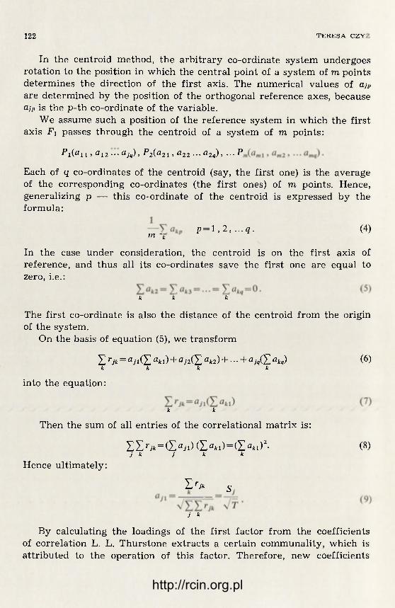
122 T E R E S A C Z Y Ż
In the centroid method, the arbi trary co-ordinate system undergoes rotation to the position in which the central point of a system of m points determines the direction of the first axis. The numerical values of ajp are determined by the position of the orthogonal reference axes, because clip is the p-th co-ordinate of the variable.
We assume such a position of the reference system in which the first axis Fi passes through the centroid of a system of m points:
p i («n> «12 ajq), P 2(^21» a22...a2q), ...P
Each of q co-ordinates of the centroid (say, the first one) is the average of the corresponding co-ordinates (the first ones) of m points. Hence, generalizing p — this co-ordinate of the centroid is expressed by the formula:
p=l ,2, ...q. (4) m k
In the case under consideration, the centroid is on the first axis of reference, and thus all its co-ordinates save the first one are equal to zero, i.e.:
k k k
The first co-ordinate is also the distance of the centroid f rom the origin of the system.
On the basis of equation (5), we transform
Z rJk = flji(Z a ki ) + «J2(Z ak2) + • • • + a j q (Z akq) (6) k k k k
into the equation:
k k
Then the sum of all entries of the correlational matrix is:
Z Z rjk = ( Z a j 1) ( Z « « ) = ( Z (8) j k j k k
Hence ultimately:
Z rjk s
J k
By calculating the loadings of the first factor f rom the coefficients of correlation L. L. Thurstone extracts a certain communality, which is attributed to the operation of this factor. Therefore, new coefficients
http://rcin.org.pl

M U L T I F A C T O R A N A L Y S I S IN E C O N O M I C R E G I O N A L I Z A T I O N 12,1
of correlation must be calculated; these should contain that part of the remaining communality which can be attributed to fur ther possible factors. These "residuals" are calculated from the equation:
1 rjk = rJk - an akl = a j2 ak2 + aj3ak3 +...+ ajq akq. (10)
The residuals of correlation can be treated as scalar products of pairs of vectors in a (q—l)-dimensional space. A system of m points of the following co-ordinates is obtained:
my-'in 2 J am3 > ••• amq) •
Then (q—1) co-ordinates of the centroid of m points determined by equa-tion (4) are equal to 0. The centroid is the origin of the system in a (q—1 )-dimensional space.
In order to calculate the factor loadings, i.e., to find a new centroid, the procedure of reflecting algebraic signs in a residual matrix is em-ployed 13.
The loadings of the second factor in the particular variables are established from the formula:
= (ID
in which E denotes that if variable j was reflected, the algebraic sign must be changed into the opposite one.
L. L. Thurstone develops the simple formula
q 2m +1 - v8/7 + 1 ^ 2) " 2
for the calculation of the maxmum number of factors which can be established in m variables 14.
Besides the centroid method, there are other methods closely linked to it which are based on the same principle. L. L. Thurstone gives four more methods: the diagonal method, and variants of the centroid method — the proup method, the grouping method, and the multiple group method 15.
13 The theoretical foundations and the technique of reflecting the sings were given by L. L. Thurstone, The Vectors of Mind, op. cit., pp. 95-97; 111; and by K. J. Holzinger and H. H. Iiarman, op. cit., pp. 184-186, 363—366.
14 L. L. Thurstone, The Vectors of Mind, op. cit., p. 76. :5 Cf. R. B. Cattell, Factor Analysis, New York, 1952, pp. 167—187, and B. Fruch-
ter, op. cit., pp. 52—59, 87—99.
http://rcin.org.pl
124 T E R E S A C Z Y Ż
We must also mention K. J. Holzinger's bi-factor method, C. L. Burt 's bipolar factor metod and D. N. Lawley's maximum likelihood method. All these are developments of Ch. Spearman's theory 16.
A method based on other principles than the centroid one is H. Ho-telling's and T. L. Kelley's principal components method1 7 . When the communality itself only is analyzed, i.e., when no specific factors are taken into account, this method is called the principal factor method 1S. This method makes possible the extraction of factors which explain the maximum communality and give the possibly smallest residuals in the correlational matrix. This means that the sum of the squares of the factor loadings is the largest possible for each variable. It follows that the correlational matrix can be analyzed by this method with the use of the smallest number of orthogonal factors.
The principal factor method has won the greatest recognition by mathematicians because of the univocality of its results. Therefore di-verse modifications of this method are extensively employed in psycho-logy, sociology or geography.
In this method, the reference system consists of vectors which rep-resent the variables. If the vectors of variables are perpendicular to one another, the points which represent the particular units in the case of positive correlation will dispose into a set in the form of an ellipsis. The large and the small axes of it correspond to factors. If the vector of a third variable, perpendicular to the former one, is introduced into the two-dimensional system, a three-dimensional system is obtained, in which the set of points takes the form of an ellipsoid.
From the algebraic standpoint, the selection of the axis is equivalent to choosing factors in the decreasing order of their contributions to the communality. The analysis starts with factor F h the contribution of which to the communality is as great a total as possible. Next, the first factor residual matrix is calculated. Further , another factor F2 indepen-dent of Fi with a maximum contribution to the remaining communality is extracted. This process is continued until the whole communality has been analyzed.
16 K. J. Holzinger and H. H. Harman, op. cit., pp. 11—1-54; R. B. Cattell, op. cit., pp. 146—148; A. E. Maxwell, Calculating Maximum-likelihood Factor Loadings, Journal of the Royal Statistical Society", Series A, Vol. 27, Part 2, 1964, pp. 238— —241.
17 H. Hotelling, Analysis of a Complex of Statistical Variables into Principal Components, Journal of Educational Psychology, 24, 1933, pp. 417—441, 498—520; T. L. Kelley, Essential Traits of Mental Life, Harvard Studies in Education, 26, 1935, Cambridge, Mass, quoted, by K. J. Holzinger and H. H. Harman, Factor Ana-lysis, Chicago, 1941, p. 155.
1S K. J. Holzinger and H. H. Harman, op. cit.
http://rcin.org.pl

M U L T I F A C T O R A N A L Y S I S IN E C O N O M I C R E G I O N A L I Z A T I O N 12,1
The description of the mathematical foundations of the principal factor solution is a follows 19.
If the linear form of m variables is given
Zj=ajiF1+cij2F2 + ... + ajqFq ( / = 1 , 2 , . . . m) (13)
the communality of the variable j is:
h) = a2n+a)2 + ...+a%, (14)
where ajx determines the contribution of factor Fj in the communality of variable j.
The sum of the contributions of the first factor F^ to the communaliti-tes of m variables
A1 = a2ll+all+all + .. 2+aml. (15)
The solution of the problem consists in finding such values of the co-efficients a;i for which assumes the maximum value, the following condition being fulfilled:
rjk = r'jk= Y,ajpakP j , k = l , 2 , . . . m (16) p=i
p = 1,2, ...q
By employing Langrange's method of undetermined multipliers for establishing the conditional extremum, the following set of m equations is obtained:
(/i?-A)tfn + r12a2l+ r 1 3 a 3 1 + . . .+ rlmami=0
r2iali+(hl-X)a2i+ r23a3l + ...+ r2maml= 0 (17)
'ml «11+ rm2a2l+ rm3a3l + ...+(hf„-X)aml=0
These equations constitute the bases for the calculation of the unknown coefficients ah.
A necessary condition for the solution of this set of equations is that the determinant of the coefficiennts an must be equal to 0.
Thus,
1(J Ibid., pp. 159—168, 322—323; H. H. Harman, Modern Factor Analysis, Chi-cago, 1960.
http://rcin.org.pl

126 T E R E S A C Z Y Ż
(hl-X) ri2 r 1 3 . . . r l m
r 2 1 (/?! — A) 7*23 ••• ''2m
>*31 7-32 (hl-A)...r3m
rm 1 rm2 rm3 ••• 0}m ~
= 0 (18)
This is a characteristic equation, in which all roots are real. By substituting one of the roots of the characteristic equation for X in
(17), we obtain a system of (m — 1) hemogeneous linear equations. This system of equations has a number of solutions, all of which are propor-tional to one particular solution. It follows from the analysis of the
m maximization A1 that the factor of proportionality Aj = £ aJ1=A1. Hence
j= i A, is equal to one of the characteristic roots of the equation, namely to the largest root h . The largest root h of equation (18) is introduced into (17) and a solution is obtained: <xn a21 aml. Next, in order to fulfil the relationship (15), these values are divided by the square root of their squares and multiplied by J ?.i. In this way, the following formula is developed:
a J l \ / A 1 " " - 7 = 1 , 2 ,
V a f l + a 2 1 + a m l m (19)
H. Hotelling also introduced a simplified method of calculating factor loadings in solving the main factor. He used an approximate determina-tion of the characteristic roots by the iteration process method without the previous development cf the characteristic determinant 20.
The set of factor loadings obtained in effect of the extraction of fac-tors by a a definite method is not the only possible, but it is a definite set of these loadings determined by a definite position of the reference system. Because the principal configuration of vectors is an invariable element, the projections of this constant configuration upon differently positioned systems of reference can be mutually transformed and, in this sense, they are equivalent (provided, though, that the origin of the system of co-ordinates is not dislocated, but that the reference system undergoes a rotation around this point).
The problem of the rotation of reference vectors emerges when an interpretation of the significance of the factors is attempted. It has been stated that there is on definite position of the reference system which
20 Cf. K. J. Holzinger and H. H. Harman, op. cit., pp. 184—186, 363—366.
http://rcin.org.pl
M U L T I F A C T O R A N A L Y S I S IN E C O N O M I C R E G I O N A L I Z A T I O N 12,1
yields a set of factorial loadings of particular significance and corresponds to the real factors, whereas all other positions are mathematical transfor-mations of it. The actual position of the reference system, which corres-ponds to the real factors, can be found in the course of the rotation of the factioral matrix. The procedure of rotation consists in multiplying the matrices of the previous factorial loadings by the transformation matrix, which containts the direction cosines of the new axes in relation to the unrotated factors. The establishment of the most appropriate position of the reference system is one of the most difficult problems of factor ana-lysis. According to Thurstone, in case of rotation it is a principle of pro-cedure to endeavour after the so-called simple structure 21. The "simpli-city" of such a structure of factor loadings consists, in this case, in that each variable has the relatively smallest contents, i. e., a predominant loading of some single factor, and, conversely, only some of the variables under analysis are measures of the given factor. The establishment of the simple structure is therefore of considerable importance for an interpretation of the factors obtained 22.
It must be observed that none of the methods of extracting factors gives results which could be recognized as final without rotation. In fact, C. L. Burt maintains that the bipolar factor method and the bi--factor method render systems of loadings directly siutable for interpre-tation 23. D. J. Whery also studies factor solution without rotation 24. Ho wever, R. B. Cattell takes a different view in this respect: he thinks the process of rotation is indispensable in all cases 25. That in to say, the facto-rial matrix obtained by the principal factor method should also be trans-formed into a matrix of factors rotated in accordance with the principles of the rotation process. But B. J. L. Berry omits this transformation, pro-ceeding directly to rotation to simple structure using the normal varimax criterion, thus simplifying he mathematical procedure in the analysis 26.
Factor analysis carried out by the principal factor method yields the factorial matrix A of order m X q , which contains the loadings of q factors in m variables. Matrix A fulfils the equation:
21 L. L. Thurstone, 1935, op. cit., pp. 150—163. 22 It must be observed that the problem of "designating" the factors in sciences
employing empirical indexes (psychology) differs from that in the sciences em-ploying ex definitione indexes (economic geography).
23 R. B. Cattell, op. cit., p. 66. 24 R. J. Wherry, Hierarchical Factor Solutions without Rotation, Psychome-
trika, Vol. XXIV, No 1, March 1959, pp. 45—51. 25 R. B. Cattell, op. cit., p. 66. 26 B. J. L. Berry, The Mathematics of Economic Regionalization, in: Economic
Regionalization, Prage 1966, pp. 7—20.
http://rcin.org.pl

128 T E R E S A C Z Y Ż
R = A-A' and A'A = A (20)
A is a diagonal matrix consisting of values of the characteristic roots /, connected with every factor. The characteristic root contains that part of communality which is explained by each of q fundamental factors. Mo-reover, by virtue of the equation
F = Z- A-A~1 (21)
the matrix F is calculated. Every element ftp of this matrix is a so-called factor score, i. e., the value given to unit i by virtue of factor p.
The matrix of factor scores F is a starting point for the proper group-ing of areal units into classes of homogenous areas in relation to q fun-damental sets of communality.For this purpose, dimensional analysis based on the method of individaul points is applied 27. It consists in treat-ing the areal units which are included in the set as points of a multidi-mensional space (q-dimensional), when these units are studied in rela-tion to q factors). A definite set of individual points corresponds to any set of units which is examined in relation to a given system of features.
The distance between units i and j in a q-dimensional Euclidean space is a measure of a multifeature similarity of the areal units. The matrix of distances D of order n X n contains distances between each point and all other points. In virtue of the matrix of distances the grouping of the areal units into classes of maximum homogeneity is carried out.
B. J. L. Berry calculates the distance between units i and j according to the formula 28:
¿¡j = VX (fiq ~~fjq)2- (22)
R. Stone presents in a more detailed manner a method of establishing distances based on Euclid's conception 29. A set of areal units can be also ordered by J. Czekanowski's method of linear arrangement, or by help a Wroclaw dendrite 30.
27 J. Perkal, O zbiorach punktów materialnych i abstrakcyjnych w badaniach przyrodniczych (On sets of material and abstract points in natural studies) Sprawozdania Wrocławskiego Towarzystwa Naukowego, 12, Series B — Supplement, 1957.
28 B. J. L. Berry, op. ext., p. 27. 29 R. Stone, A Comparison of the Economic Structure of Regions Based on the
Concept of Distance, Journal of Regional Science, vol. 2, 1960, pp. 1—20. 30 J. Perkal, Matematyka dla rolników (Mathematics for agriculturists), Part I,
Warszawa, 1958, pp. 71—82; B. Kopociński, Dyskryminacja za pomocą dendrytów (Discrimination by help of dendrites), Zastosowania Matematyki, Vol. V, No. 3, 1960, pp. 271—279.
http://rcin.org.pl

M U L T I F A C T O R A N A L Y S I S IN ECONOMIC REGION A L I Z A T I O N 12,1
It must be emphasized that the methods mentioned above tend to lead to a typological classification of fundamental areal units (because of the absence of spatially continuous groupings of all similar units). In delimit-ing regions, such a meta-feature as the position of units of a definite type must be additionally taken into account31 .
*
The application of the taxonomic method based on multifactor analysis in economic geography and in other socio-economic sciences is fully justified. In the endeavour to attain a full knowledge of reality, it is necessary to reduce the manifoldness of the complex socio-economic phe-nomena. Factor analysis, which starts f rom a large number of variables, discovers the factors that are at the roots of the co-variation. These fac-tors, in the field of the socio-economic phenomena, are impossible to be perceived in practical research activities. By introducing a small number of fundamental dimensions, factor analysis facilitates research operations in a reduced space of properties.
The calculation technique in the extraction of factors is essentially the same, no matter whether psychological, sociological or geographical variables are concerned.
However, the situation differs essentially when we attempt an inter-pretation of the factors obtained. In this case, we proceed from statistical problems to the substantial questions of a given science. Do the factors, which constitute certain structures, represent a set of real variables in the field of socio-economic phenomena? The interpretation of factors is to a large extent predetermined by the theoretical or conceptual con-struction which the student thinks to be the most relevant. The interpre-tation of factors introduces therefore some arbitrariness into factor ana-lysis. The principles of the interpretation of the extracted factors in the socio-economic sciences evoke considerable doubts. Most often it is examined to what degree are the factors obtained representative of the primary features. In effect, one obtains a basis for estimating the cha-racter of the main factors and for determining the significance of the particular primary features in the differentiation between the units.
In sociological research, M. J. Hagood applied factor analysis in the study of the level of living of farmers in the particular counties of the USA in 1945 32. She selected four mutually correlated features, which
31 A region is a spatially coherent area of maximum internal homogeneity. 32 M. J. Hagood and D. O. Price, Statistics for Sociologists, New York, 1957,
pp. 526—528.
9 G e o g r a p h i a P o l o n i c a t . 15 http://rcin.org.pl

130 T E R E S A C Z Y Ż
reflected the level of consumption of the farmer family, and by the principal factor method established the loadings of one common factor in the particular variables33 . She calculated an index of the level of living for the particular counties, which she expressed by the formula:
IU) = wllLZi + w2lZJ2 + w31 Z{ + vv4 x Z{ (23)
where Zj = (X^ —M,) : Si denotes the normalized value of feature i in county j, XJ
t = value of feature i in county j, Mi = mean value of feature i, •Si = standard deviation of feature i, Wi i = loading of factor in the particular variables.
On the basis of factor analysis, D. O. Price established the funda-mental dimensions of metropolitan centres 34. By help of four factors he explained the correlations in the variation of 15 features for 93 towns. Having at his disposal "the accumulated knowledge and judgements on forces at play in metropolitan centres", he identified the factorial load-ings obtained as (1) the degree of maturity of city, (2) the extent to which a city is a service centre, (3) the level of living within a city, (4) the per capita trade volume of a city.
C. A. Moses and W. Scott made a typological classification of Great Britain's towns by means of multifactor analysis 35. The 60 variables cha-racterizing the 157 towns from the socio-economic standpoint were re-duced to 6 factors, which expressed altogether 69 per cent of the com-munality of the primary features. The authors made a preliminary esti-mation of the character of 4 principal features, which constituted the bases for the classification of towns, and they called the first factor the social differentiation factor, the second and third — the stage of develop-ment factors (the second referred to 1931-50, the third to the period after 1950), and the fourth — the overpopulation of dwellings factor.
P. O. Pedersen made multifactor studies of the population structure of the Copenhagen metropolitan area by identifying 5 principal factors:
33 M. J. Hagood in her works introduces the principle of using only those factors which explain more than 10 per cent of the communality of features. Most often he takes into account one factor.
34 D. O. Price, Factor Analysis in the Study of Metropolitan Centers, Social Forces, vol. 20, May, 1942, pp. 449—455.
35 C. A. Moser and W. Scott, British Towns. A Statistical Study of Their So-cial and Economic Differences, Centre for Urban Studies, Report No. 2, XII, Lon-don, 1961.
http://rcin.org.pl

M U L T I F A C T O R A N A L Y S I S IN E C O N O M I C R E G I O N A L I Z A T I O N
urbanization, socio-economic status and growth and change 36. Ch. T. Jo-nassen and S. H. Peres used factor analysis in sociology to discover sets of communality which constituted the bases of the interdependencies bet-ween the features of systems of communities 37. As initial data these au-thors used the values of 82 variables measuring aspects of community Kfe in 88 counties of Ohio. They employed L. L. Thurstone's group method, as modified by R. J. Wherry. In this manner, the particular communities were defined in terms of only 7 factors, which were called: (1) urbanism, (2) welfare, (3) influx, (4) poverty, (5) magni-complexity, (6) educational effort, (7) proletarianism.
By the same method, S. Rokita studied the living conditions of the population of the province of Cracow, and discovered the operation of three factors: the recreation factor, the industrialization factor and the urbanization factor 38.
Factor analysis was also used by W. L. Garrison and D. F. Marble in their study of transportation network. They analyzed the connection matrix of the Venezuelan air transport system in 1957. By the linear transformations method the matrix of order 59X59 was reduced to a ma-trix of order 59 XT (r,<C59). By an interpretation of the four principal factors, which explained 38 per cent of the total variation observed in the network, certain structural relationships within the transport system were identified.
M. Megee studies the applications of factor analysis in the researches in economic growth and development3 9 . She starts from the assumption that factor analysis as a statistical method which allows for the use of a larger number of features makes possible quantitative researches in macro-economic development4 0 . M. Megee analyzed the matrices of the economic developments of the USA and Mexico by applying the new technique M which allows for the study of the changes in time of the relative weight of the factors. She identifies the extriected factors: e. g., in her analysis for the year 1960 in Mexico she defines the principal factors
33 P. O. Pedersen, An Empirical Model of Urban Population Structure. A Factor Analytical Study of the Population Structure in Copenhagen. Proceeding of the First Scandinavian — Polish Regional Science Seminar, Committee for Space Econ and Regional Planning Polish Ac. Sc., Studies, vol XVII, Warszawa 1967, pp. 193— —214.
ii7 Ch. T. Jonassen and S. H. Peres, Interrelationships of Dimensions of Com-munity Systems. A Factor Analysis of Eighty-two Variables, Columbus. 1960.
38 S. Rokita, Analiza czynnikowa w badaniach regionalnych (Factor Analysis in regional studies), Przeglqd Statystyczny, vol. XIII, No. 3, 1966, pp. 245—260.
39 W. L. Garrison and D. F. Marble, Factor-analytic Study of the Connectivity of a Transportation Network. Papers, vol. XII, 1964,, pp. 231—238.
40 M. Megee, op. ext., pp. 187—209.
9* http://rcin.org.pl

132 T E R E S A C Z Y Ż
as "irrigation and energetics industry", "energetics industry and urba-nization", "chemical industry", "expenditures on education and invest-ments".
M. J . Hagood also applied factorial analysis in the delimitation of agriculture-population regions of the USA 41. She started by grouping 104 features, which characterized the demographic and agricultural relations in the particular states, into 14 classes. On the basis of a factorial ana-lysis of each of the 14 correlational matrices, the loadings of the first factor in the variables of the particular classes were identified. Next, 14 indexes for each of the 48 states were calculated, and the values of the correlation coefficients of all pairs of these indexes were established. The factor analysis of this correlational matrix made possible the construction of a composite index for each state. In turn, the states located in the same interval of the composite index were grouped into regions. However, in M. J. Kagood's opinion, there is no certainty in the operation of grouping that neighbouring states will be joined together, since the units in one interval might not always form a contiguous grouping. For this reason, M. J. Hagood introduces additionally a coefficient of similarity in the s t ructure of the states by calculating the correlations between the values of 104 features for each pair of states.
In his studies on the world's economic development, B. J. L. Berry showed that by help of factor analysis 43 variables applied in the cha-racteristics of the economic development of 95 countries could be re-duced to 4 principal components which accounted for 94 per cent of the variance. The following are the factors of the world's economic deve-lopment: (1) technological scale, (2) demographic scale, (3) contrast in income and external relations, (4) the large and the small (countries). B. J . L. Berry completed a regionalization, on the basis of the values of tihe 4 principal components of variance as related to the particular countries 42. He also applied the factorial analysis method in the regional division of the USA: 9 statistical districts of the U.S. with features con-cerning 6 categories of services were grouped into 4 multifeature regions,
41 M. J. Hagood, Statistical Methods for Delineation of Regions Applied to Data on Agriculture and Population, Social Forces, vol. 21, March 1943, pp. 288—297; Cf. also M. J. Hagood, D. O. Price, op. cit., pp. 541—546. It must be remarked that in the field of regionalization this mathematical-statistical procedure in the form of an experiment was for the first time used by M. G. Kendall (cf. his study on The Geographical Distribution of Crop Productivity in England, Journal of the Royal Statistical Society, Series A, vol. 102, 1939, pp. 21—62.
42 B. J. L. Berry, An Inductive Approach to the Regionalization of Economic Development, in Norton Ginsburg (ed.), Essays on Geography and Economic De-velopment, Department of Geography Research Papars, No. 62, The University of Chicago, 1960.
http://rcin.org.pl

M U L T I F A C T O R A N A L Y S I S IN E C O N O M I C R E G I O N A L I Z A T I O N 12,1
which were uniform by virtue of the basic patterns of variation 43. By this method, he also delimited the areas of "rural poverty" in the Ca-nadian state of Ontario and the economic regions of India 44.
On the basis of the short survey of the current applications of factor analysis in economic geography and sociology it must be said that, actually, only certain hypotheses concerning the nature of extracted factors can be formulated. In fact, only psychology has the possibility of verifying them by way of fur ther experiments. In economic geography as well as in other socio-economic sciences we are usually unable to subject hypotheses to empirical control, because we do not know the em-pirical meaning of the indexed phenomena which we use in analysis. Within these sciences we use, as a rule, definitional indicators. As a matter of fact, the problem of the interpretation of factors in economic geography and sociology has not been solved yet and requires fu r the r studies. Because of the fact that, in the socio-economic sciences, the nature of factors can be determined in a provisional manner only, one may across the question whether we should not abandon the "designating" of factors and leave them in the form of statistical quantities. However, in this situation, i. e., in the case of the absence of attempts at the interpretation of factors, factorial analysis applied in economic regionalization will not produce any definite set of criteria by virtue of which general economic regions in the form of certain underlying elements of some fundamental structure could be delimited; factorial analysis is a mere mathematical convenience in the procedure of economic regionalization.
43 B. J. L. Berry, A Method for Deriving Multi-Factor Uniform Regions, Przegląd Geograficzny, Vol. XXXIII, No. 2, 1961, pp. 263—282.
44 B. J. L. Berry, The Mathematics of Economic Regionalization, op. cit., pp. 7—20.
http://rcin.org.pl

http://rcin.org.pl
G E O G R A P H I A P O L O N I C A 15
A G R A P H T H E O R Y I N T E R P R E T A T I O N O F N O D A L R E G I O N S
J O H N D . N Y S T U E N AND M I C H A E L F . D A C E Y
The purpose of this paper is to describe a procedure for ordering and grouping cities by the magnitude and direction of the flows of goods, people, and communications between them. Current theories of nodal regions and central place hierarchies provide the bases for the recogni-tion of regionwide organization of cities into networks. These two the-ories were developed by students who recognized that the direction and magnitude of flows associated with social processes are indicators of spatial order in the regional structure of urban society. Whether the flow is local and to the city's hinterland, or regional and to the rank ordering of cities, the notion of central or nodal point is dependent upon the levels of strongest associations within the total flow 1.
The present problem is to develop a method capable of quantifying the degree of association between city pairs in a manner that allows identification of the networks of strongest association. These associations may be in terms of interactions that occur directly between two cities, or indirectly through one or more intermediary cities. The magnitude of the combined direct and indirect associations is measured by an index that is related to certain concepts of graph theory. This index is used to identify the degree of contact between city pairs and it provides a quantitative basis for grouping cities. The resulting subgroups of cities are analogous to nodal regions. When each city in a study region is as-signed to a subgroup, it is possible to specify the rank ordering of cities and to evaluate the functional relations of the nodal hierarchy.
1 B. J. L. Berry and W. L. Garrison, A note on Central Place Theory and the Range of a Good, Economic Geography, Vol. 34, 1958, pp. 304—311. E. L. Ullman, A Theory for Location of Cities, American Journal of Sociology, Vol. 46, 1941, pp. 853—864. D. Whittlesey, The Regional Concept and the Regional Method, American Geography: Inventory ar.d Prospect, P. C. James and C. F. Jones (eds.), Syracuse University, Syracuse, 1954.
http://rcin.org.pl
136 JOHN D. N Y S T U E N A N D M I C H A E L F. D A C E Y
In this paper, pertinent geographic and graph theoretic concepts are discussed and are then used as a basis for deriving the method isolating noidal regions. While this method is illustrated by the use of intercity telephone calls in Washington state, the techniques are quite general and may be adapted to many types of phenomena. A particular pheno-menon is suitable for this type of analysis when it may be viewed as a relationship or flow that links objects that are properly mapped as points. In the present illustration, cities are conceptualized as puncti-form elements in a telephone network. Other suitable areas of appli-cation include the flow cf information or material products between business firms in a metropolitan area, the flow of mail or freight between cities in a region, the interpersonal relations between the inhabitants of a city or the political structure that connects federal, state and local governments.
R E L A T I O N S H I P T O E X I S T I N G T H E O R Y
Cities may be viewed as nuclei of specialized activities which are spatially concentrated and functionally associated. Each activity has its own set of associations outside the city. To account for the many dif-ferent external connections of each specialization, general statements concerning urban associations must be multi-dimensional. Accordingly, urban hinterlands are normally defined by establishing a boundary from a composite of the spatial range of several central place functions, such as the trade area of the local newspaper, the extent of wholesale drug distribution, bus passenger volumes, governmental jurisdiction, and similar indices of central place functions.
Long-distance telephone communications may be considered a single index of this multi-dimensional association among cities. A grouping of cities on the basis of telephone data defines only a network of telephone traffic centers. The validity of interpreting these telephone traffic cen-ters as an accurate indicator of multifunctional associations depends upon a correspondence of the hinterlands which are developed with those obtained from studies which evaluate many types of contacts. The authors are willing to accept that telephone flows are one of the best single indices of all functional contacts. It has an advantage over the use of a series of indices because it obviates weighing the individual contri-butions of the several indices 2.
2 C. Hammer and F. C. Ikle, Intercity Telephone and Airline Traffic Related to Distance and the Propensity to Interact, Sociometry, Vol. 20, 1957, pp. 306—316;
http://rcin.org.pl

G R A P H THEORY I N T E R P R E T A T I O N OF N O D A L REGIONS 137
T H E N O D A L R E G I O N O R H I N T E R L A N D
Nodal regions are defined by evaluating the external contacts of small areal units. Each of these areal units is assigned to that place with which it has the dominant association. Usually, this will be a nearby city, and this city is defined as the central place or nodal point for the unit areas oriented to it. The aggregation of these unit areas, is called the nodal region.
This does not deny the existence of other flows or associations to and from each areal unit. Such flows do exist so that each areal unit is connected to many other cities. Newspaper circulation, for example, may be dominated by the local daily while the nearest metropolitan paper may also be well represented, and The New York Times may find its way into a few homes in the area. Also, many sporadic contacts with former hometown papers may be present. Nevertheless, the "dominant association" remains the critical concept in defining a nodal structure. The remaining non-dominant associations are not used, even though the magnitudes of some of these associations may be relatively large.
T H E H I E R A R C H Y O F C I T I E S
The nodal region describes the relationship between the hinterland, which is areal, and the central or nodal city, which is punctiform. Clearly, there is no loss of generality by considering only paired con-tacts between points. In the hinterland concept, the areal units may be abstracted to the level of points so that the association is in terms of many points being linked to a single central point3 .
The hinterland of a major metropolitan center, such as Chicago, may encompass a large region and incorporate many of the region's functions. The strongest of the flows between Chicago and its hinterland are point to point associations of the cities within the region. At this scale, the relationship between nodal regions and the hierarchy of central places becomes clear. The major hinterland of Chicago is defined by its do-minant association with many smaller metropolises. Each of these centers, in turn, is the focus of association from other, smaller centers within its immediate vicinity. These associations incorporate lower order functions than those establishing direct associations to Chicago. In this fashion
C. D. Harris, Salt Lake City: A Regional Capital, University of Chicago, Chicago, 1940, E. L. Ullman, Mobile: Industrial Seaport and Trade Center, University of Chicago, Chicago, 1940.
3 For example see: W. Tsard and D. J. Ostroff., General Interregional Equ-ilibrium, Journal of Regional Science, Vol. 2, 1960, pp. 67—74.
http://rcin.org.pl

138 J O H N D. N Y S T U E N A N D M I C H A E L F. D A C E Y
city regions are nested together, intimately dependent upon the range of the functions which define the associations at each level.
A hierarchy of cities of this type may be reduced to an abstract net-work of points and lines. The points represent the cites while the lines represent the functional associations. Though a myriad of lines exists in the network, there is present a basic structure of strongest associations which creates the nested nodal regions and the hierarchy of cities. Both the direct and indirect associations are important in these intercity struc-tures. In terms of the direct associations, for example, a wholesale es-tablishment may receive orders directly and ship directly to some points within the system. Alternately, the associations are indirect when the orders are accumulated at various levels of the hierarchy and proceed upward to the regional headquarters. In the same manner, the outbound shipments from the central city proceed down the ranks to intermediary levels through middlemen, rather than directly to every point in the region.
Many associations are of this indirect type. For instance, political control moves up and down the ranks, rather than through direct com-munication between the national party leaders and the ward leaders. Most commodities are assembled and distributed through a hierarchical structure within the organization. This results, in part, f rom the eco-nomies of moving large lots over long distances and, in part, f rom the better control it affords over the operation. In evaluating the entire fa-bric of urban society, it is evident that subtle, indirect influences and associations are frequently exerted by one location on another. A system of analysis which accounts for both the direct and the indirect associa-tions between cities is appropriate.
In summary, the nodal region is defined on the basis of the single strongest flow emanating from or moving to each of the unit areas in the vicinity of a central place. The region is delimited by the aggrega-tion of these individual elements. The hierarchy of central places is de-termined by the aggregation of the smallest central places which are dependent upon a single, larger center for the functions they lack. This nesting of cities defines the organization of networks of cities and the position of each city within the network. Such nesting depends upon the available bundle of functions and the relative dominance of bundles.
In this study we start with the cities and towns of a large area. Then, the structure of association among the cities is specified by assigning each city to one of several subgroups. By considering the system as a set of points and lines, where the lines represent the association between points, certain theorems of linear graphs become evailable for the ana-lysis of the functional association of cities within an area.
http://rcin.org.pl

G R A P H THEORY I N T E R P R E T A T I O N OF N O D A L REGIONS 139
A GEOGRAPHICAL APPLICATION OF SOME GRAPH THEORY CONCEPTS
Graph theory is a mathematics of relations. By specifying certain properties of the relations between cities and accepting the point-line abstraction of graph theory, certain theorems become available for analyzing intercity flows 4. Consider the cities in a region as a set of points. Consider, also, a line joining a pair of points whenever there exists a certain flow between the cities they represent. The finite col-lection of points and lines, where each line contains exactly two points, is a linear graph of the relations established by the flows.
S O M E C H A R A C T E R I S T I C O F L I N E A R G R A P H S
A point is called adjacent to another point if it is connected to it by a line. The network of lines is the only information contained within the graph. Scalar distance and direction, the most striking aspects of geographical maps, are not defined for a graph. If the relationship is of equal value for every connected pair, the graph is a binary graph. Most graph theory relates to this type of construction which simply indicates whether a line (a relation) exists or does not exist between any pair of points. The connections, however, may be considered to have intensity. Intensity is displayed on the graph by assigning a value to the lines.
Orientation of a relation between two points is displayed on the graph by an arrowhead a->b, and read "a is related to b". A graph which spe-cified orientation is called a directed graph or digraph. The relationship between two points on a directed graph need not be symmetrical and, when intensity of the connection is defined, the intensity may be dif-ferent for each direction.
A path f rom the points a to e is a collection of points and lines of the form, a, a->b, b, b-+c, . . ., cL, d->e, e, where the points a, b, . . . , e, are distinct. A sequence is a collection of points and lines from a to e in which the intermediate points need not be distinct. A graph is weakly
4 Some general statements of graph theory are: D: Konig, Theorie der End-lichen und Unendlichen Graphen, Leipzig, 1936 (reprinted by Chelsea Publishing Col, New York, 1950); C. Berge, Theorie des Graphes et Ses Applications, Dunod, Paris, 1958; F. Harary, Unsolved Problems in the Enumeration of Graphs, Publi-cations of the Mathematical Institute of the Hungarian Academy of Sciences, Vol. 5, series A, 1960, pp. 63—95; Some Historical and Intuitive Aspects of Graph The-ory, Siam Review, Vol. 2, April 1960, pp. 123—131. The utility of graph theory for geographic analysis has been demonstrated by W. L. Garrison, Connectivity of the Interstate Highway System, Papers and Proceedings of the Regional Science As-sociation, Vol. 6, 1960, pp. 121—137.
http://rcin.org.pl

140 JOHN D. N Y S T U E N A N D M I C H A E L F. D A C E Y
connected if there exists a path between each pair of points, disregarding orientation. The points in a component of a graph are weakly connected and are not connected to any other points in the graph. The degree of a point is the number of points to which it is adjacent. In a directed graph a point has an out-degree and an in-degree depending on the orientation of the lines incident to it.
M A T R I X N O T A T I O N
For every linear graph there is an adjacency matrix which completely describes the graph, and vice versa. The matrix notation is convenient for arithmetic manipulation. Every point in a graph is represented by a row and a column of the matrix. The element, oca, of the adjacency matrix takes the value of the line; if it exists, between the points i and j; if the line does not exist, the value of the xa is 0.
The diagonal elements, xa, of the adjacency matrix represent the re-lation of each point to itself. This relationship may or may not be de-fined. When it is not defined, all elements of the main diagonal are, by convention, put equal to zero.
P R O P E R T I E S O F T H E D O M I N A N T R E L A T I O N S B E T W E E N C I T I E S
The geographic theory reviewed above suggests that within the myriad relations existing between cities, the network of largest flows will be the ones outlining the skeleton of the urban organization in the entire region. The term "largest" implies an oriented relation because a flow between a pair of cities may be the largest in terms of one city but not necessarily in terms of the other city. The relation "largest f low" may have various definitions, such as the largest out-flow, in-flow, or total flow. The present example uses the number of out-going intercity telephone messages from each city to every other city in the study area. It is possible to construct a directed graph of these relations. Using the principle of dominant association, a single out-directed line is assumed to be associated with each point. When number of telephone messages are used to measure intensity of intercity associations, this assumption is easily accepted because for any city the largest volume to any one city is typically several times greater than the next largest message flow. An assumption of this type is tenable only for intercity relations which may be ranked or have a unique, largest interaction. In other situations, nodal region is most likely an inappropriate concept.
The collection of largest flow lines between city pairs defines a net-work of orientation among the points. Where each point has a largest
http://rcin.org.pl

G R A P H THEORY I N T E R P R E T A T I O N OF N O D A L REGIONS 141
flow ; that largest flow may be found by simple inspection of a matrix of flows between all pairs, and it is the maximum element in each row when the matrix displays number of messages from the row city to the column city. The present intention is to use this notion of largest flow to aggregate cities associated with a central place. The resulting aggre-gation is said to be composed of the "subordinates" of the central city. The problem is the recognition of a "central city". In order to establish a "dominant center" three additional properties of the "largest f low" relation are now identified.
One property states that a city is "independent" if its "largest f low" is to a "smaller city". A small city remote f rom large metropolitan cen-ters may display this type of independence because its largest flow is to an even smaller, nearby city. Conversely, in the same region a large satellite city closely associated with a metropolitan center does not have this independence because its largest flow is to the metropolis. So, to identify independent cities a measure of size is required. Size may be externally assigned, e.g., by population of each city; or it may be in-ternally assigned, e.g., by the total volume of messages to or from all cities in the region. In the example below size is assigned in accordance with the total inmessage flow from all cities in the study region. This value is the column total of the matrix of flows between all pairs of cities. In these terms, an "independent" or "central city" is defined as one whose largest flow is to a smaller city. A subordinate city is a city whose largest flow is to a larger city. This assumes ni ambiguities arise to obscure the dominate (largest) city of a pair. This occurs when largest flows are reflexive, that is, two cities whose largest out-connections are to each other.
A second property is transitivity. This property implies that if a city a is subordinate to city b and b is subordinate to c, then a is subordinate to c.
A third property stipulates that a city is not a subordinate of any of its subordinates. A graph showing this relation is called acyclic. It is easily seen that an acyclic graph contains a hierarchy.
T W O T H E O R E M S
The largest flow from every subordinate city is called the nodal flow. These flows form the nodal structure of the region and (for the particular relation under study) this skeleton displays the functional association of the cites in a region. This structure is analogous the nodal region and contains a hierarchy of centers. It is important to recognize that in this nodal structure the out-contact from at least one point is zero. This par-
http://rcin.org.pl

142 J O H N D. N Y S T U E N A N D M I C H A E L F. D A C E Y
Blank spaces represent zero elements.
•Terminal point. **Trivial terminal point.
Fig. 1. Graph of a nodal structure in a region (hypothetical)
ticular case is called a terminal point and in terms of an urban structure, this type of point is interpreted as a central city.
The following statements are useful deductions concerning the graph of a nodal structure. Figure 1 illustrates the resulting concepts.
(1) The components of a nodal structure partition the set of cities. Proof. Each city is represented by a point in a graph of a nodal struc-
ture. Each point is weakly connected to every point in its component
http://rcin.org.pl

G R A P H T H E O R Y I N T E R P R E T A T I O N OF N O D A L REGIONS 143
and to no point not in its component. A trivial component is an isolated point. Each point is, therefore, assigned to one and only one component. Such as assignemnt of a set is a partitioning.
(2) Each component of a nodal structure has a unique central city (terminal point).
Proof. Every path has at least one subordinate point and also a point to which all points on the path are subordinate by the transitive pro-perty of the relation. If this point is subordinate lit must be adjacent to a point not on the path because the relation is acyclic. Upon extending the path, an end point with zero out-degree will be found in the com-ponent because at least one point is in the component and is not subor-dinate 5. This end point is the only terminal point to which all points on the related paths are subordinate because no branching occurs on any path (every subordinate point has an out-degree of one).
Now assume distinct paths in a component and extend the paths to their terminal points. Any other point connected to a point in one ex-tended path h^s no other connection because each point has an out--degree no greater than one. If their terminal points were distinct, the subgraphs associated with distinct paths by the method described would not be connected in any way. This contradicts the fact that all elements in a component are weakly conected. Therefore, each extended path must have the same terminal point.
I N T E R P R E T A T I O N O F T H E N O D A L S T R U C T U R E
The nodal structure may be used to distinguish groups of cities that have maximum direct linkages and the rank order of these cities may be calculated. The hinterland of the central city may also be determined by mapping the cities in a nodal structure and then drawing a line just beyond the cities which are most distant f rom the central city. In ac-cordance with existing theory, the hinterland or nodal region contains the area in which the maximum association or flow is toward the central or nodal city. In addition, this plotting schows the hierarchy over which the central city is dominant.
A N E X T E N T I O N O F T H E T H E O R Y T O I N D I R E C T A S S O C I A T I O N S
The operations and structure that has been described evaluates only direct contacts between city-pairs. It does not incorporate the indirect associations, and these, conceivably, could be very influential in deter-
5 Here, only finite graphs are considered.
http://rcin.org.pl

144 JOHN D. N Y S T U E N A N D M I C H A E L F. D A C E Y
mining functional associations. Admittedly, direct contacts should re-ceive the greater weight, but some evaluation of the indirect channels between city-pairs would seem appropriate because of the indrect as-sociations which occur within a hierarchy. Indirect associations may be evaluated by using matrix manuipulations to adjust the nodal struc-ture. It is postulated that the increment of indirect association of in-fluence decreases with increases in the length of the channel.
P O W E R S E R I E S O F T H E A D J A C E N C Y M A T R I X
The first step in accounting for indirect influence is to adjust the raw data matrix so that the direct association between each city-pair is some proportion of the total association of the largest center in the area. This is accomplished by obtaining the maximum column total of the adjacency matrix (max £xa) and dividing every xn element by this summation. Put :
i ya — ocij/max Zxa. The following inequalities result for a graph of n
j points:
0£yu<l ( i , j = l,2,...,n) (1)
0 < 5 > l 7 ^ l 0 ' = 1 , 2 , . . . , n) . (2) j
The maximum column total equals 1. The linear graph corresponding to this adjacency matrix has the
appropriate, positive, decimal loading. Let the adjacency matrix be cal-led Y. In terms of linear graphs, the power expansions of Y have inte-resting interpretations. The matrix Y2, which is obtained by Y Y under usual matr ix multiplication, describes a graph when all sequences have a length of 2. The length of a sequence is the number of lines it contains. Further , the loading of the lines of each sequence of length 2 are obtained by multiplication. Since of initial loadings are decimal values, an attenuated value is associated with a contact that proceeds f rom point i to j through a sequence of lenght 2. The surae of all such two-step sequences f rom i to j is the value of all possible indirect contacts of length 2.
This assertion may by demonstrated as true by considering the mea-ning of the summation:
a i j = Yjk yikykj (k = l , 2, n) (3)
and where an is an element in Y2. The yik is the loading on the line from point i to point k in the graph
and the ykj has the same meaning for the link f rom k to j. The only
http://rcin.org.pl

G R A P H T H E O R Y I N T E R P R E T A T I O N OF N O D A L REGIONS 145
terms which enter the summation are those where a sequence of length 2 exists. When a link from or to the kth point does not exist, the whole term is zero. The an is the total value of all sequences of length 2. In a similar manner it may be shown that the elements of Y3 specify the attenuated value of all sequences of length 3, and so on. The meaning of the following summation is clear:
B=Y+Y2+Y3 + ... + Y"+... (4)
The element, ha, of B represents the total direct and indirect influence from i to j.
Some examples may be useful. Given the cities a, b. . . ., n, a typical sequence f rom a to e might be a->b->c-+d->e. Imagine an activity in city a as having influence cn a respondent in b, this b in turn contacts a respon-dent in c, and continuing until a small response in e is affected. The pro-bability of such a chain of occurrence depends, in part, on the magnitude of the flows in every link of the sequence. In general, the longer the sequence, the more remote is the probability of a response and when a response occurs it is less intense.
Alternatively, the flow of influence may be re-channeled through the same city more than once. For example, a sequence may have the form a->b a->e. All such summations are included in the matrix B.
The summation of the power expansion of Y is not demonstrated to be the correct form of the attenuation of flows in a sequence. It is ex-tremely doubtful that the matrix B is the most appropriate measure-ment of the total direct and indirect influences. It is essentially a mea-sure of chance indirect contact. The distribution of actual indirect asso-ciaton is very likely not at all random but rather concentrated in certain flow channels, in which case the matrix B would be an underestimate of indirect influence. It does, however, have a greater appeal than the ma-trix Y which incorporates only the direct influences. The choices of the particular power expansion is dictated by the ease of its computation. Several other methods may also be appropriate 6.
C O M P U T A T I O N O F T H E P O W E R S E R I E S O F T H E A D J A C E N C Y M A T R I X
A convenient method of computing the matrix B is to use the fol-lowing identity:
( 1 - Y ) _ 1 = 1 + Y+Y2 + ... + Y" + ... (5)
G For examples see, R. D. Luce nad D. Perry, A Method of Matrix Analysis of Group Structure, Psychometrika, Vol. 14, 1949, pp. 95—116; and L. Katz, A New Status Index Derived from Sociometric Anadysis, Psychometrika, Vol. 18, 1953, pp. 39—44.
10 G e o g r a p h l a P o l o n i c a t . 15
http://rcin.org.pl
146 JOHN D. N Y S T U E N A N D MICHAEL F. D A C E Y
and then: fi = ( l - y ) " 1 - l , (6)
where the 1 is the indentity matrix. The inverse, (1—Y)—1, is known to exist if the inequalities (1) and (2) hold.
T H E N O D A L S T R U C T U R E O F M A T R I X B
The nodal structure of matrix B is established by isolating the net-work of largest flows in the same manner as was described for the direct associations. Because the associations enumerated in matr ix B are adjusted for both direct and indirect flows, it is expected that a more reasonable structure is obtained.
AN EXAMPLE
Washington State was chosen as the study area. The utility of the nodal s tructure concept is evaluated by choosing a set of cities in this area and then determining the nodal structure that prevails. The nodal, s tructure which emerges should resemble the known hinterland and ranking of the major cities in the area. Certain cities outside of the State were included in the study in order to examine the role they play in the network of city associations. Portland, Oregon and Vancouver, British Columbia were especially important additions.
The associations were defined by the number of long distance tele-phone messages between city-pairs during one week in June, 1958 7. Certain cities were omitted f rom the study due to characteristics of the data and in order to limit the size of the study.
Many pairs of neighboring cities have direct dialing service and in these instances the intercity calls were not recorded in long distance data. Dormitory towns for Seattle and several "twin cities" such as Aberdeen-Hoquiam, Chehalis-Centralia and Pasco-Kennewick had direct--service exchange. This is not a serious deficiency in the data because such cities very likely function as a single point in the state-wide net-work, anfcl orie of the "twin cities" in each pair could be used in the study. Certain fair ly large cities north of Seattle and along the Puget Sound were omitted for lack of data. These cities were serviced by
7 We are indebted to the Pacific Bell Telephone and Telegraph Company and especially to Mr. Homer Moyer, a Seattle officer of that company, for this in-formation.
http://rcin.org.pl

G R A P H T H E O R Y I N T E R P R E T A T I O N OF N O D A L R E G I O N S 147
a different telephone company. Because each year the telephone com-panies simultaneously take a one-week sample of intercity telephone calls, comparable data exist but there was no attempt to obtain them. Finally, all cities above a certain pupulation size were not included in order to restrict the size of the study. Some small towns were chosen, how-ever, in an effort to obtain samples of hierarchies with directed paths
of length 2 or more. The map in Fig. 2 identifies the cities in the study. With the advantage of hind-sight, it might have been preferable to have included more small towns in the study.
Certain channels of communication are omitted because they are not recorded in the long distance data. Direct-line calls are an example. Probably the only large volume, direct-line in the state links Seattle wi th Olympia, the state capital. If these data were included, the maxi-m u m association of Olympia might shift f rom Tacoma to Seattle. Though beyond the scope of this study, interesting results could be obtained if all channels of communication were included, such as radio, telegraph, mail and messenger service.
10* http://rcin.org.pl
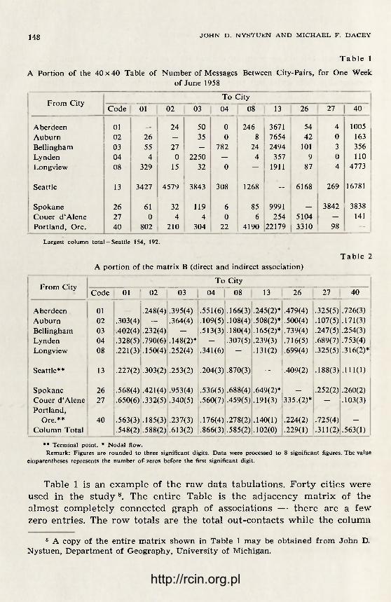
148 JOHN D. N Y S T U E N A N D MICHAEL F. D A C E Y
Table 1
A Portion of the 40 x 40 Table of Number of Messages Between City-Pairs, for One Week of June 1958
From City To City
From City Code 01 02 03 04 08 13 26 27 40
Aberdeen 01 24 50 0 246 3671 54 4 1005 Auburn 02 26 — 35 0 8 7654 42 0 163 Bellingham 03 55 27 — 782 24 2494 101 3 356 Lynden 04 4 0 2250 — 4 357 9 0 110 Longview 08 329 15 32 0 — 1911 87
•
4 4773
Seattle 13 3427 4579 3843 308 1268 - 6168 269 16781
Spokane 26 61 32 119 6 85 9991 — 3842 3838 Couer d'Alene 27 0 4 4 0 6 254 5104 — 141 Portland, Ore. 40 802 210 304 22 4190 22179 3310 98 -
Largest column total —Seattle 154, 192.
Table 2 A portion of the matrix B (direct and indirect association)
From City To City
From City Code 01 02 03 04 08 13 26 27 40
Aberdeen 01 — .248(4) .395(4) .551(6) .166(3) .245(2)* .479(4) .325(5) .726(3) Auburn 02 .303(4) - .364(4) .109(5) .108(4) .508(2)* .500(4) .107(5) .171(3) Bellingham 03 .402(4) .232(4) - .513(3) .180(4) .165(2)* .739(4) .247(5) .254(3) Lynden 04 .328(5) .790(6) .148(2)* .307(5) .239(3) .716(5) .689(7) .753(4) Longview 08 .221(3) .150(4) .252(4) .341(6) — .131(2) .699(4) .325(5) .316(2)*
Seattle** 13 .227(2) .303(2) .253(2) .204(3) .870(3) - .409(2) .188(3) .111(1)
Spokane 26 .568(4) .421(4) .953(4) .536(5) .688(4) .649(2)* — .252(2) .260(2) Couer d'Alene 27 .650(6) .332(5) .340(5) .560(7) .459(5) .191(3) 335.(2)* - .103(3) Portland,
Ore.** 40 .563(3) .185(3) .237(3) .176(4) .278(2) .140(1) .224(2) .725(4) —
Column Total .548(2) .588(2) .613(2) .866(3) .585(2) .102(0) .229(1) .311(2) .563(1)
** Terminal point . * Noda l flow. Remark: Figures are rounded to three significant digits. Da t a were processed to 8 significant figures. The value
einparentheses represents the number of zeros before the first significant digit.
Table 1 is an example of the raw data tabulations. Forty cities were used in the s tudy 8 . The entire Table is the adjacency matrix of the almost completely connected graph of associations — there are a few zero entries. The row totals are the total out-contacts while the column
8 A copy of the entire matrix shown in Table 1 may be obtained from John D. Nystuen, Department of Geography, University of Michigan.
http://rcin.org.pl

G R A P H T H E O R Y I N T E R P R E T A T I O N OF N O D A L R E G I O N S 149
totals are the total in-contacts. The direction of the message flow is read from the "row" city to the "column" city. The main diagonal entries are zero by convention.
Table 2 is the adjacency matrix B which evaluates both the direct and indirect associations between the cities 9. The nodal structure contained in this matr ix was determined by (1) identifying the nodal flow, (2) ranking the cities by their total incoming associations, (columns
Fig. 3. Matrix of the nodal structure
totals), (3) assigning an orientation from cities with smaller total asso-ciations to one with a larger total association and (4) identifying the non--oriented cities as the center of its hierarchy. Figure 2 shows the re-sults. Figure 3 is the adjacency matrix of the nodal structure derived form the direct and indirect associations.
9 The computations were made possible by a grant of computer time from Western Data Processing, University of California at Los Angeles.
http://rcin.org.pl
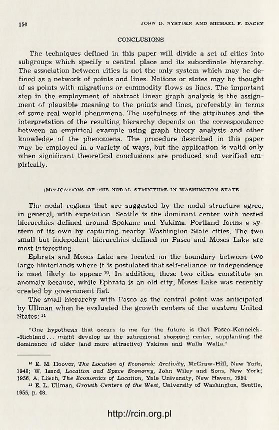
150 JOHN D. N Y S T U E N A N D MICHAEL F. D A C E Y
CONCLUSIONS
The techniques defined in this paper will divide a set of cities into subgroups which specify a central place and its subordinate hierarchy. The association between cities is not the only system which may be de-fined as a network of points and lines. Nations or states may be thought of as points with migrations or commodity flows as lines. The important step in the employment of abstract linear graph analysis is the assign-ment of plausible meaning to the points and lines, preferably in terms of some real world phenomena. The usefulness of the attributes and the interpretation of the resulting hierarchy depends on the correspondence between an empirical example using graph theory analysis and other knowledge of the phenomena. The procedure described in this paper may be employed in a variety of ways, but the application is valid only when significant theoretical conclusions are produced and verified em-pirically.
I M P L I C A T I O N S O F T H E N O D A L S T R U C T U R E I N W A S H I N G T O N S T A T E
The nodal regions that are suggested by the nodal structure agree, in general, with expetation. Seattle is the dominant center with nested hierarchies defined around Spokane and Yakima. Portland forms a sy-stem of its own by capturing nearby Washington State cities. The two small but indepedent hierarchies defined on Pasco and Moses Lake are most interesting.
Ephrata and Moses Lake are located on the boundary between two large hinterlands where it is postulated that self-reliance or independence is most likely to appear J0. In addition, these two cities constitute an anomaly because, while Ephrata is an old city, Moses Lake was recently created by government fiat.
The small hierarchy with Pasco as the central point was anticipated by Ullman when he evaluated the growth centers of the western United States:1 1
"One hypothesis that occurs to me for the future is that Pasco-Kenneick-- R i c h l a n d . . . might develop as the subregional shopping center, supplanting the dominance of older (and more attractive) Yakima and Walla Walla."
10 E. M. Hoover, The Location of Economic Arctivity, McGraw-Hill, New York, 1948; W. Isard, Location and Space Economy, John Wiley and Sons, New York; 1956. A. Lösch, The Economics of Location, Yale University, New Haven, 1954.
11 E. L. Ullman, Growth Centers of the West, University of Washington, Seattle, 1955, p. 48.
http://rcin.org.pl

G R A P H T H E O R Y I N T E R P R E T A T I O N OF N O D A L REGIONS 151
The effect of the national border is clear. Vancouver is subordinate to Seattle and it does not dominate any city in the study, even though it is a large city and is much nearer to Lynden and Bellingham than is Seattle. It is probable that Vancouver would have been a terminal point of other Canadian cities had been included within the study. This is not a defect in the method. The results are only an evaluation of the associations between the cities in the study.
The nodal region of Tacoma, a large city south of Seattle, is also anti-cipated by theory. Tacoma is dominant in a nearby region. This region if off-center, in the direction away from the larger city of Seattle. The dominance of Seattle re-asserts itself at even greater distances so that Aberdeen and Centralia are directly associated with Seattle, rather than by a two-link path through the closer and larger city of Tacoma 12. This and the other agreements with existing theory and accepted empirical evidence demonstrate the utility of the nodal structure for analyzing city associations.
F U R T H E R G R A P H T H E O R Y A P P L I C A T I O N S
Given a set of cities in an area and a measure of association between thern, a set of hierarchies has been obtained. Even more information is desirable. Spokane is obviously the second most important central place in Washington state, yet it is subordinate to Seattle in a hierarchy while the much smaller places of Moses Lake and Pasco dominate their respec-tive systems. Intuitively, a second in command position in a large orga-nization is more important than the primary position in a tiny organi-zation. Some measure of this difference in status is desirable. A fur ther applicatin of graph theory to this problem is suggested in a paper by Harrary 13. His ideas are adapted to this problem by the present authors in a fu r the r study of city associations.
12 E. M. Hoover, op. cit.; W. Isard, op. cit.; A. Lösch, op. cit. 13 F. Harary, Status and Contrastatus, Sociometry, Vol. 22, 1959, pp. 23—43.
http://rcin.org.pl

http://rcin.org.pl

G E O G R A P H I A P O L O N I C A 15
REGIONALIZATION OF PENNSYLVANIA COUNTIES FOR DEVELOPMENT PLANNING
B E N J A M I N H . S T E V E N S AND CAROLYN A . B R A C K E T T
DEVELOPMENT P R O G R A M S AND ALTERNATIVE REGIONALIZATIONS
The social nad economic problems of declining and underdeveloped areas in the U.S. have led to a complex of policies and programs designed to deal with these issues. Because of the structure of American gouvern-ment, these programs have had to be applied at the state or local level. Many of the problems have a regional dimension, however, which extends beyond established government boundaries.
This need not necessarily create difficulties. Similar programs can be and have been established simultaneously in contiguous states or counties in both the ARA and Appalachian programs. But it is not clear that the replication of similar programs 'in several different contiguous jurisdictions is either the most efficient use of federal resources or the most effective way to generate economic frowth.
A D V A N T A G E S O F P L A N N I N G A N D D E V E L O P M E N T R E G I O N S
There are at least two reasons why development planning, admi-nistration, and expenditure might be more effective if applied to larger areal aggregates. First, the similarity of problems among several coun-ties in the same state or contiguously located in two or more states may lead to efficiencies if a single program can be planned, administered, and financed for the counties as a group. The simple reduction in du-plication of effort might be the minimum benefit to be derived.
Second, wasteful competition among conuties may be avoided by coordinated planning. If each county has its independent plan and pro-gram, and the counties are similar in location advantages, the result may be a fairly even distribution of new economic activities. With the limitation of the number and size of potential activités, no one of the counties may receive enough new employment to generate sustained
http://rcin.org.pl

154 BENJAMIN H. STEVENS A N D C A R O L Y N A . B R A C K E T T
growth and the possibilities of a single integrated industrial development may be lost. Associated with this loss may be the additional loss of the agglomeration economies which come with industrial concentration and which can lead to accelerated growth. Similarly, economies of scale in training and educational programs, public works projects, and the like, may go unutilized. In general, the effectiveness of the funds expended may be seriously reduced by lack of integrated planning.
P O L I T I C A L P R O B L E M S I N R E G I O N A L P R O G R A M S
Integrated planning, of course, requires a recognition of the linkages which already exist among local areas, or those which might be encou-raged through complementary development programs. Such planning entails difficult political decisions since an integrated approach is very likely to lead to higher growth rates in certain local areas than in others, especially in the short run. Nevertheless, the welfare impacts of develop-ment programs may be very substantially enhanced if there are actually spillover and diffusion effects of development. Local areas surrounding the "development center" in a region will probably be better off in the long run. Still the political difficulties of implementing integrated de-velopment plans should not be underestimated.
U S E S O F A L T E R N A T I V E R E G I O N A L T Y P E S
Integrated planning and programming on a multi-county regional basis requires the determination of the optimal areal composition of regions. At least three types of regionalizations are possible 1. First are homogeneous regions which have common characteristics both in their problems and potentialities. This type of regionalization should be most useful in increasing efficiency by replacing duplicate administrations for similar programs in the several counties with a single administration for the whole region. However, homogeneous regions, since they tend to be uniform in economic strength, separate healthy and weak econo-mies into separate regions. This may not lead to the most effective
1 Relevant references are: Brian J. L. Berry, A Method for Deriving Multi--Factor Uniform Region: Przegląd Geograficzny, 33, 1961, pp. 263—282, and Iden-tification of Declining Regions: An Empirical Study of the Dimensions of Rural Poverty, in Richard S. Thoman (ed.), Areas of Economic Stress in Canada. Queen's University, Kingston. G.A.P. Carrothers, An Historical Review of the Gravity and Potential Concepts of Human Interaction, Journal of the American Institute of Planners, 22, 1956, pp. 94—102.
http://rcin.org.pl

REGION A L I Z A T I O N OF P E N N S Y L V A N I A COUNTIES 155
development plans, but should concentrate attention on county groups which are economically weak and separate out those regions which are stronger.
Nodal regionalization, which is based on the strength of inter-county linkages, emphasizes economic, social, and political interdependencies. Plans which concentrate efforts in the nodal center depend upon the linkages to generate multiplier effects in hinterland counties of the re-gion. These counties probably will grow at a slower rate in the early stages of development than they would in a homogeneous region plan.
A growth pole regionalization is based on the demonstrated growth potential of particular counties with which weaker counties would be associated in planning regions. This is actually a variation of the nodal region approach, since it depends on spillover and diffusion effects f rom the growth pole to generate secondary development in counties asso-ciated within the same region. The difference between growth pole and nodal regionalization lies in the characteristics of the pole or node. Nodal regionalization simply groups, in the same region, counties which are most strongly linked to the nearest node. Growth pole regionalization, on the other hand, recognizes both the strength of the linkages and the economic growth potential of the node.
C O M P A R A T I V E A D V A N T A G E S O F A L T E R N A T I V E R E G I O N A L I Z A T I O N S
Both nodal and growth pole regions provide administrative and plan-ning efficiencies. The linkages which exist between the node or pole on the one hand and the tr ibutary areas on the other are partly in the form of communication linkages. The dependence of the hinterland on the central place for information, financial services, and the like increases the effectiveness of the node as an administrative center. This depen-dency reinforces the agglomeration economies enjoyed by the central place and, hence, increases its effectiveness as an administrative center.
From the strictly political point of view the homogeneous region appears to have distinct advantages. A cooperative effort among counties which will share equally in development is probably easier to establish than a program which concentrates development in a node or pole. Since the node or pole, already has some economic strength it should grow much more rapidly leaving the tr ibutary counties at an increasing disadvantage in the short run. The use of the growth pole approach may actually imply an accelerated decline of areas far f rom the pole as popu-lation and activities move to locations with better access to the center. For such areas substantial growth may come only after the polar center
http://rcin.org.pl

156 BENJAMIN H. STEVENS A N D C A R O L Y N A . B R A C K E T !
has grown to a size at which there is a spillover of people and industry. The nodal or growth pole approach should eventually lead to greater benefits for all. To the extent that this approach can be made politically feasible, it should probably be encouraged in those areas where a strong node or pole exists.
R E G I O N A L S I Z E A N D C O M P A C T N E S S
The question of regional size is closely connected with the issues raised above. Regions can be too large to be planned and administered effectively: They can also be too large for effective plan implementation because of the necessity for close cooperation and extensive personal efforts of business and political leaders. Areas which feel themselves to be too far away to participate ful ly in development may not lend either the time or energy necessary to make the program work. Growth pole regions especially can be too large if development diffusion occurs beyond the planning horizons of the leaders in the fringe areas.
On the other hand, regions can be too small to support an efficient planning and administrative effort. Furthermore, nodal or polar regions which do not include strongly linked outlying counties may lead to unrealistic or workable development plans.
A cJosely related problem is that of compactness. At the very least, each county in a region must be contiguous to one other county in the same region. But communication ease, and hence greater administrative efficiency, results when more counties are mutually contiguous, or conti-guous to the center of the region. Furthermore, close geographic ties may facilitate the implementation of plans. For nodal and polar regions, economic, social and political linkages tend either to imply geographic linkages or to substitute for them. Since linkages tend to weaken with distance, it can be expected that nodal and polar regions will be relati-vely compact although the form of the major transportation network, historical linkages, and topography may cause certain anomalies. Homo-geneous regions, which may lack these linkages, must depend more on close geographic association.
PROBLEMS OF CRITERIA AND MEASUREMENT IN REGIONALIZATION
The formation of development planning regions is not a simple matter even after the type of regionalization has been decided upon. Cri-teria must be devised to measure homogeneity, nodality, and growth
http://rcin.org.pl

REGION A L I Z A T I O N OF P E N N S Y L V A N I A COUNTIES 157
potential; data must be assembled to apply the criteria; and techniques must be available or devised to group areas into regions, based on the selected criteria. The goal of the entire procedure is to achieve a "best" set of regions for development planning purposes.
H O M O G E N E O U S R E G I O N S
The problem of useful criteria of measurement is probably the least tractable. Of the vast array of criteria which could be used to define homogeneous regions, it is difficult to determine which would best serve to define homogeneity for planning purposes. The best single criterion might be political homogeneity because this would maximize the proba-bility that plans would be adopted and implemented. However, homo-geneity in industrial structure, per capita income, or level of unemploy-ment might be best f rom the economic viewpoint. Or f rom the social point of view, educational level, religion, or country of origin might be selected.
Fortunately, there are often strong intercorrelations among many of the possible political, economic, and social variables which might be used. This means that similar regionalizations could result f rom the use of different criteria. Nevertheless, the problem of criteria selection should still be carefully considered. It may be that the best criterion of homo-geneity for planning purposes is a measure which is not highly corre-lated with the criteria current ly in use. The identification of the critical criterion will then depend on the success of the plans and programs which are applied to experimentally-derived regions.
N O D A L R E G I O N S
The selection of criteria of nodality presents similar problems: there are many types of linkages between counties which might be measured. Again, however, there is often a high level of intercorrelation among the measures. A county which gets its newspaper f rom a neighboring county will probably also carry on some of its business and do some of its heavy shopping there. The strength of these intercorrelations is more difficult to measure than that of socioeconomic variables however. Until more linkage data is available, the question of the best criteria of nodality remains a problem in central place theory.
http://rcin.org.pl

158 B E N J A M I N H . S T E V E N S A N D C A R O L Y N A. B R A C K E T T
G R O W T H P O L E R E G I O N S
The identification of growth poles is probably the most difficult prob-lem, both theoretically and empirically. In part, it is not clear whether growth potential is best measured by past growth or by other variables which might describe preconditions for growth. Even if agglomeration economies are important in accelerating growth, it can still be conjec-tured that growth follows a logistic pat tern and that an economy which has been growing will not enjoy as fast a rate of growth as one in which development is just starting.
On the other hand, diffusion and spillover effects may spread sooner f rom nodes which have already enjoyed growth and which have reached some threshold size, even if they are no longer growing rapidly. And places which have not been growing or which have actually declined may be growth poles if they are large enough.
After all, the most significant spillover and diffusion effects occur around major metropolitan centers which are themselves declining economically.
Furthermore, there is the problem of defining growth itself. Per capita income, employment, population, value added in manufacturing, and other measures of growth have been suggested as "best". These measures seem to be somewhat interccrrelated, but they are clearly not perfect substitutes. A viable theory, or system of theories, of the nature and determinants of urban growth has not been developed and tested. And even less is known about the diffusion of growth from a central point into its t r ibutary region. Further research will be required before the best criteria for growth and the identification of growth poles can be established.
TECHNIQUES OF REGIONALIZATION
The problem of grouping a large number of units into a smaller num-ber of regions can be approached on at least two levels. An intuitive approach, based on a small number of measurements and a good general understanding of the areas involved, is in many ways easiest. Geogra-phers have traditionally delimited regions by mapping techniques combi-ned with subjective evaluation. Such simple approaches may still be best in some circumstances.
But there are o number of reasons why systematic and computerized techniques may be preferable. It is difficult to achieve an optimal regio-nalization, no matter what the criteria, without extensive and repetitive computation. The difficulty of this computation increases rapidly with the
http://rcin.org.pl

REGION A L I Z A T I O N OF P E N N S Y L V A N I A COUNTIES 159
number of elements to be grouped. Furthermore, the growing availability of data leads to the possibility of using a large number of measures singly or in combination. This requires factor analysis and other statis-tical techniques to reduce the large mass of undigested data to manage-able number of meaningful measures. Finally, there is often a need to make alternative regionalizations of the same type, or regionalizations which are some weighted combination of types. This is simply not practi-cal without computerized techniques.
M U L T I - F A C T O R H O M O G E N E O U S R E G I O N A L I Z A T I O N
The currently-used technique for homogeneous regionalization is based on factor analysis. As developed by Berry (see above), this techni-que has become simple, straightforward, and easily applicable. A variety of socioeconomic variables are measured for the several areal units. Fac-tor analysis combines these measures, many of which tend to be highly intercorrelated, into independent factor measures. The size of the diffe-rences in the scores of the areal units on these factors is then used as measures of similarity of the areas.
Homogenous regionalization proceeds by grouping those elements which have the minimum differences, on average, in their factor scores. Generally all factors are weighted equally although a minor refinement of the technique allows different weights for different factors. Fur ther -more. certain factors can be left out in the regionalization if the criteria of homogeneity are better expressed by a single factor or a smaller set of factors.
The technique, at each step, either pairs two units, adds another unit to a group which has been formed at an earlier step, or combines two previously formed groups. In the latter case, significant discontinuities can occur in the size of regions as expressed by the number of units combined in any single group. Unfortunately attempts to constrain the system so that there will be a maximum size of region or a reasonable variance in regional size lead to difficult questions about the optimality of the regionalization which finally results. By preventing a unit f rom joining a region or two regions f rom joining each other, the system might produce a final result in which homogeneity could be improved. Unfortu-nately it is not easy to discover, at the end of the process, what changes in the regionalization would cause improvement or how large the im-provement would be. Methods will have to be developed to measure what the losses in homogeneity might be before the placing of regional size constraints on the technique could be considered acceptable.
http://rcin.org.pl

160 BENJAMIN H. STEVENS A N D C A R O L Y N A . B R A C K E T T
At present this problem is avoided by one of two methods: either the process is halted at the step at which two regions would otherwise com-bine to form one oversized region; or large regions in the final result are arbitrarily split up. The latter approach is easier because the process, if left alone, will eventually combine all units into one single region. Since the regional composition at each step is printed in the final result, it is possible to select ex post the step at which the regionalization looks „right" f rom the point of view of the mean and variance of regional size. If the right stopping point includes a small number of very large regions with the rest of roughly equal size, the larger ones can then be split up.
Unfortunately, the best stopping point is generally a compromise be-tween restricting large regions and avoiding single-element regions. Cer-tain areas which are most unlike their neighbors will tend to remain iso-lated until the later steps of the regionalization procedure. By this point some regions may have grown overly large. Again, the only proce-dure available so far is to make the most acceptable compromise and then adjust by hand.
N O D A L R E G I O N A L I Z A T I O N
Nodal regionalization can be performed by methods essentially the same as those described above. The difference lies in the variables to be entered into the factor analysis. In nodal regionalization, these would be linkage variables which measure the strength of various types of in-teractions between regions. Otherwise, the basic technique is the same as that used for forming homogenous regions.
There is however an important conceptual difference between the procedures. Homogenous regions are formed f rom units which are mu-tually as similar as possible whereas nodal regions are formed from units which are closely linked to a central place or node, but which are not necessarily linked to each other. One implication of this difference is that nodal regionalization is much more susceptible to handicraft methods. Not only are linkages easier to map than similarities, but the economic and social structure of natural regions is such that a less-developed county is likely to be much more strongly linked to one particular cen-tral place than to any other.
Furthermore, since linkage data is much more limited in both quan-tity and quality, few measures of nodality are ordinarily available. Be-cause one purpose of factor analysis is to reduce a large number of inter-correlated measures to a much smaller number of independent factors, factor analysis is not usually employed in nodal regionalization. Never-
http://rcin.org.pl

REGION A L I Z A T I O N OF P E N N S Y L V A N I A COUNTIES 161
theless, factor analysis and computerized grouping, which are essential to homogeneous regionalization, will become more important for nodal problems as a wider range of linkage data becomes available.
G R O W T H P O L E R E G I O N A L I Z A T I O N
Systematic growth pole regionalization techniques have not previously been developed. A linear programming technique, developed for the purposes of this study, is described in some detail in Appendix 1. Briefly, the technique links in an optimal manner „sources" of growth, which are the weaker and tributary counties. Aside from the problems of defining and measuring growth potential, the use of this technique raises a num-ber of questions.
First, it is not clear how small or compact a region should be in order to enjoy growth diffusion throughout the region even in the long run. As applied so far , the technique bases the size of region on the relative strength of the growth pole and relative weakness of the tr ibutary coun-ties. But this can lead to very large regions if the pole appears to have significant potential and the surrounding counties have only slight growth weaknesses. Furthermore, the technique may group into a region counties which are not directly contiguous to the pole but lie in the se-cond or third ring of counties around the pole. Further research will be necessary before it is known whether this makes any sense.
Second, the criterion of optimality which has been used is the simi-larity on the basis of factors other than growth of the spillover counties to the polar county. On the basis of the previous discussion it is now questionable whether this is the best criterion. Preferable alternatives might be the strength of nodal linkages to the pole or the degree of homogeneity of the tributary counties with each other rather than with the pole. Theoretically, a growth pole almost be definition should be different from its tributary area but close linked to it. Both theoretical and empirical research, as well as refinement of the technique itself, will be necessary to resolve these issues.
COMBINATIONS OF TECHNIQUES
It appears that some of the questions raised in the previous discussion could be best answered by combining techniques. For example, a growth pole region should be compact and made up of a growing node together with the areas which are both closely linked to the node and similar to one another. The need for this combination of approaches and criteria has led to the development of a new computer technique which preliminarily
11 G e o g r a p h i a P o l o n i c a t . 15
http://rcin.org.pl

162 BENJAMIN H. STEVENS A N D C A R O L Y N A . B R A C K E T T
serves the purpose. This method is outlined briefly here and described in some detail in Appendix 2.
The philosophy of the new method is that growth potential, homoge-neity, nodality, and compactness are disparate criteria. Therefore, any technique which attempts to take them all into consideration must allow for arbitrary relative weighting of these criteria. In other words, the investigator must decide how much compactness he is willing to give up to achieve a higher degree of homogeneity; or how important he feels linkage is relative to homogeneity. The technique thus proceeds by com-bining at each step those elements which have a minimum weighted sum of differences on socioeconomic factors, of measures of the interareal physical distance, and of the negative or inverse of strength of linkage. By varying the weights on the criteria, almost continuous variation of regionalization can be achieved. At one extreme, with zero weights on compactness and nodality, the technique gives the usual multifactor ho-mogeneous regions. At another extreme, with zero weights on the so-cioeconomic factors, a set of strictly nodal regions is obtained.
Although the technique has only been used experimentally, it seems to have great promise. One interesting possibility is to identify growth poles and then use the technique to force alternative regionalization around the poles. For reasons explained previously, it has not been con-sidered desirable to restrict the method to minimum or maximum num-bers of elements per region. Nevertheless the compactness criterion, based on physical distance and the „shape" of region, should tend to keep regions from becoming too large, if it is given a heavy enough weight. Further experimentation will be necessary before the technique is considered thoroughly practicable.
REGIONALIZATION OF PENNSYLVANIA COUNTIES
The counties of Pennsylvania (Fig. 1) were regionalized by the multi-factor homogeneous region technique, by handicraft nodal region techni-ques, and by the new growth pole regionalization techniques outlined above and described in Appendix 1. The results will have to be considered suggestive rather than definitive, part ly because of the limitations of the techniques and data, and partly because of he important conceptual and theoretical questions which remain to be answered.
H O M O G E N E O U S R E G I O N A L I Z A T I O N S
Data on the thirty-six social, economic, and political variables used are presented in Table 1. The selection of variables was partly a matter
http://rcin.org.pl

R E G I O N A L I Z A T I O N O F P E N N S Y L V A N I A C O U N T I E S 163
of judgment and partly of data availability, although there was a relative freedom of choice because of the mass of information made available by the State.
As was expected, many of the variables were highly intercorrelated as indicated by the intercorrelation matrix in the IBM printout attached to this report. The factor analysis, also attached, was carried up to the point at which ten factors were isolated. Beyond this point the explanatory
Fig. 1. Pennsylvania counties with code numbers
power of fu r ther factors would have been insignificant. At each level, two-factor, three-factor, etc., an attempt was made to characterize the factors on the basis of the scores of the original variables on them. This is always a dangerous procedure but it does seem necessary when factors must be selected for the regionalization procedure. And in any case, the factors have little intuitive appeal unless they are interpreted.
The results of this procedure are presented in Table 2. Note that the characterization of factors changes at each level of factorization. This is quite typical of the procedure, particularly where rotated factors are used to get the best fit. Also included in the table are the numbers of the factors used in each regionalization and the number of the map on which the corresponding regionalization appears. The factor selection for the regionalization procedure was both a matter of judgment and an at tempt to produce a variety of alternative regionalizations based on different criteria.
n» http://rcin.org.pl

Table 1
Data used in factor analysis of Pennsylvania counties
1 2 3 4 5 6 7 % Adults
% Popula-tion urba-
nized 1960
Persons/ square mile
1960
Population potential
1960
Sale in state liquor per capita
1962
with more
than 4 years high
school 1960
% Non-white 1960
Public assist-
ance per capita 1963
Adams 21.6 98.1 .58191 10.2 31.7 .7 13.67 Allegheny 93.2 2230.9 .73735 33.9 42.3 8.3 32.59 Armstrong 23.2 121.2 .56436 15.6 32.2 1.1 23.91 Beaver 70.9 469.3 .61832 23.7 37.7 5.4 14.93 Bedford 8.7 41.8 .52547 12.3 31.2 .4 27.62
Berks 64.3 318.8 .68201 20.2 31.7 1.8 12.00 Blair 68.3 258.5 .54048 16.3 37.0 .9 23.15 Bradford 30.5 47.9 .52030 11.3 41.1 1.2 32.07 Bucks 75.3 500.1 .87401 20.5 46.9 1.9 3.97 Butler 29.3 144.4 .57978 14.9 41.0 .5 12.46
Cambria 60.6 292.5 .55073 18.7 33.9 1.8 31.87 Cameron 44.8 19.0 .49539 22.8 48.6 .2 10.59 • Carbon 64.0 130.6 .65195 19.2 31.3 Л 17.17 Centre 41.2 70.5 .52401 13.6 50.0 1.0 12.27 Chester 43.8 277.1 .74642 27.9 48.1 8.4 7.81
Clarion 13.3 62.5 .52531 13.9 37.4 .1 20.27 Clearfield 28.4 71.3 .51639 11.8 32.8 .3 33.44 Clinton 40.0 41.7 .51906 11.7 39.9 .1 22.93 Columbia 45.3 110.5 .58657 12.4 38.5 .2 18.82 Crawford 32.1 76.7 .51623 20.8 43.1 1.3 22.08
Cumberland 59.1 224.9 .57982 19.5 47.0 1.6 6.64 Dauphin 76.9 423.6 .61271 25.7 42.9 9.7 20.00 Delaware 96.0 2990.0 .98201 33.2 50.1 7.1 9.70 Elk 52.0 46.3 .49922 17.3 38.4 .1 9.82 Erie 77.1 308.7 .50570 27.3 43.3 2.8 19.63
Fayette 30.1 213.3 .56251 18.2 30.2 4.8 61.97 Forest — 10.8 .50245 — 36.6 • — 12.25 Franklin 36.5 116.9 .55141 11.7 33.7 2.0 9.30 Fulton — 24.4 .52823 08.3 26.1 .8 32.15 Greene 13.2 68.3 .54691 12.0 29.3 1.0 44.05
Huntington 28.7 44.2 .53140- 11.6 35.8 2.5 41.94 Indiana 23.8 91.4 .54794 10.9 . 34.5 .6 36.26 Jefferson 40.9 71.8 .51837 14.6 36.0 .1 27.61 Juniata — 41.0 .54857 06.3 30.6 .1 21.90 Lackawanna 89.8 516.6 .62090 26.0 36.9 .4 31.27
http://rcin.org.pl
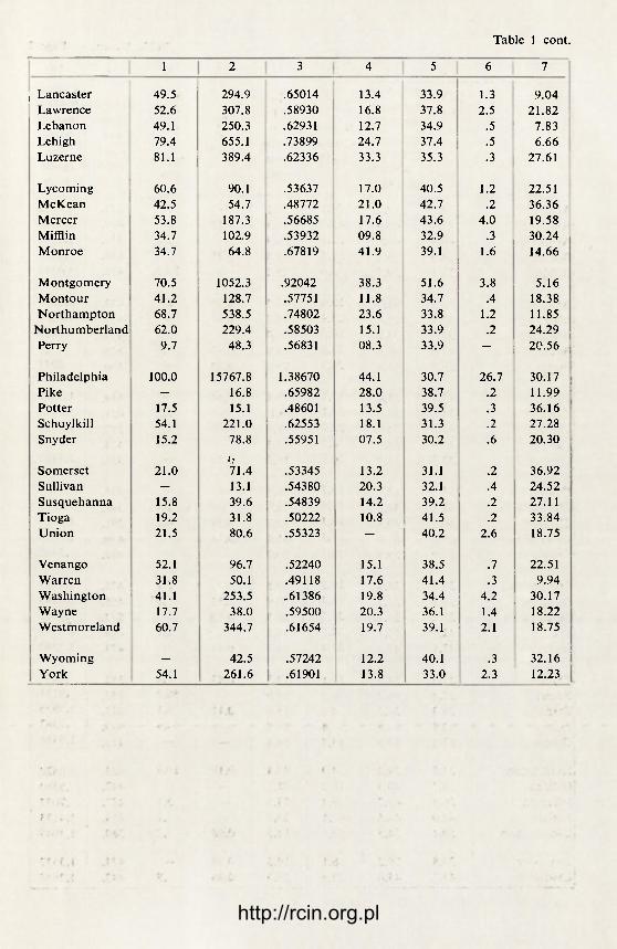
Table 1 cont.
1 2 3 4 5 6 7
; Lancaster 49.5 294.9 .65014 13.4 33.9 1.3 9.04 Lawrence 52.6 307.8 .58930 16.8 37.8 2.5 21.82 Lebanon 49.1 250.3 .62931 12.7 34.9 .5 7.83 Lehigh 79.4 655.1 .73899 24.7 37.4 .5 6.66 Luzerne 81.1 389.4 .62336 33.3 35.3 .3 27.61
Lycoming 60.6 90.1 .53637 17.0 40.5 1.2 22.51 McKean 42.5 54.7 .48772 21.0 42.7 .2 36.36 Mercer 53.8 187.3 .56685 17.6 43.6 4.0 19.58 Mifflin 34.7 102.9 .53932 09.8 32.9 .3 30.24 Monroe 34.7 64.8 .67819 41.9 39.1 1.6 14.66
Montgomery 70.5 1052.3 .92042 38.3 51.6 3.8 5.16 Montour 41.2 128.7 .57751 11.8 34.7 .4 18.38 Northampton 68.7 538.5 .74802 23.6 33.8 1.2 11.85
Northumberland 62.0 229.4 .58503 15.1 33.9 .2 24.29 Perry 9.7 48.3 .56831 08.3 33.9 — 20.56
Philadelphia 100.0 15767.8 1.38670 44.1 30.7 26.7 30.17 Pike — 16.8 .65982 28.0 38.7 .2 11.99 Potter 17.5 15.1 .48601 13.5 39.5 .3 36.16 Schuylkill 54.1 221.0 .62553 18.1 31.3 .2 27.28 Snyder 15.2 78.8 .55951 07.5 30.2 .6 20.30
Somerset 21.0 0 71.4 .53345 13.2 31.1 .2 36.92
Sullivan — 13.1 .54380 20.3 32.1 .4 24.52 Susquehanna 15.8 39.6 .54839 14.2 39.2 .2 27.11 Tioga 19.2 31.8 .50222 10.8 41.5 .2 33.84 Union 21.5 80.6 .55323 — 40.2 2.6 18.75
Venango 52.1 96.7 .52240 15.1 38.5 .7 22.51 Warren 31,8 50.1 .49118 17.6 41.4 .3 9.94 Washington 41.1 253.5 „61386 19.8 34.4 4.2 30.17 Wayne 17.7 38.0 .59500 20.3 36.1 1.4 18.22 Westmoreland 60.7 344.7 .61654 19.7 39.1 2.1 18.75
Wyoming — 42.5 .57242 12.2 40.1 .3 32.16 York 54.1 261.6 .61901 13.8 33.0 2.3 : 12.23
http://rcin.org.pl

Table 1 cont. — Page 2
8 9 10 11 12 13 14 15
% Vote Demo-
cratic for gover-
nor 1962
% Vote Demo-
cratic for state
repre-sentative
1962
V /0 Roman Catholic
1962
% Traditio-
nal Prote-stant 1962
% Jewish
1962
State park visits per
capita 1962
Expendi-tures per
pupil 1962
Capital & Liabi-lities of banks
per capita 1962
Adams 38.7 49.7 24.1 26.1 — — 475. 1.6322 Allegheny 45.8 48.6 43.7 14.5 1.15 — 499. 3.8131 Armstrong 40.3 46.9 22.6 29.9 — 5.6 436. 1.1281 Beaver 48.9 56.2 30.4 17.0 0.21 1.8 434. 1.0407 Bedford 36.1 39.7 3.8 23.2 — 24.3 470. 1.0389
Berks 44.9 51.0 15.6 41.7 0.69 2.8 470. 1.8858 Blair 33.5 39.8 23.4 23.7 0.61 — 417. 1.2139 Bradford 31.6 33.0 10.2 24.0 — .3 454. 1.3415 Bucks 40.0 40.8 25.8 18.0 0.97 .9 526. .7521 Butler 36.3 41.4 26.3 26.0 0.40 — 460. .2073
Cambria 45.4 51.4 45.1 10.8 0.64 — 449. 1.2802 Cameron 34.8 50.4 24.1 26.1 — 5.2 451. 1.7890 Carbon 45.5 54.4 32.0 41.6 — 6.4 397. 1.1768 Centre 32.6 38.5 8.5 23.3 — 6.4 478. 1.2724 Chester 32.5 33.8 20.1 19.0 0.29 — 535. 1.3889
Clarion 35.9 45.1 15.7 26.5 — 438. .5457 Clearfield 41.8 47.3 17.9 22.9 — 2.4 388. 1.1611 Clinton 40.7 40.1 13.4 23.9 0.54 4.2 391. 1.3114 Columbia 39.9 42.7 14.3 31.4 0.14 — 436. 1.6056 Crawford 37.0 39.8 15.5 20.2 — — 481. .5462
Cumberland 33.3 38.4 10.1 19.5 3.7 474. 1.1253 Dauphin 34.2 22.7 16.4 20.9 1.52 .03 458. 2.2683 Delaware 37.2 38.1 39.2 16.5 0.10 — 532. .4913 Elk 42.0 53.4 52.1 10.8 — 2.7 449. 1.5984 Erie 47.1 47.1 33.4 14.2 0.41 — 473. 1.5580
Fayette 53.3 54.9 32.1 14.3 0.43 .4 352. .8445 Forest 37.5 46.3 6.5 18.0 — 58.2 453. .4131 Franklin 38.3 38.3 4.2 18.6 0.11 6.1 433. 1.5856 Fulton 42.7 48.8 .4 26.7 — 54.9 488. .9363 Greene 53.4 63.9 13.7 19.4 — — 416. 1.9414
Huntington 34.5 39.2 4.9 42.4 0.19 10.9 483. 1.0620 Indiana 38.7 40.8 18.2 21.2 — — 447. .5560 Jefferson 36.8 43.7 16.4 23.6 — 5.1 427. .7057 Juniata 42.0 44.5 .1 35.8 — .7 414. 1.4135 Lackawanna 50.4 54.5 55.9 14.3 0.98 .2 380. 1.4945
Lancaster 28.8 28.5 8.1 19.3 0.35 — 474. 1.3537 Lawrence 43.7 45.4 29.6 29.6 0.48 .8 442. 1.2848
http://rcin.org.pl
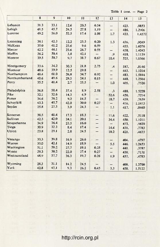
Table 1 cont. — Page 2
8 9 10 11 12 13 14 15
Lebanon 31.3 33.1 12.6 20.5 0.54 _ 423. .9853 Lehigh 41.5 45.7 24.5 27.8 1.19 — 486. 1.2906 Luzerne 49.2 56.0 52.5 17.4 1.08 1.7 433. 1.4572
Lycoming 36.1 42.3 12.2 23.5 0.20 1.3 436. .9049 McKean 35.0 41.2 23.6 9.6 0.59 — 455. 1.6076 Mercer 42.2 46.1 23.6 26.7 0.55 — 458. 1.4043 Mefflin 36.2 50.4 3.8 42.1 — .9 418. 1:1139 Monroe 39.5 50.7 9.7 38.7 0.67 10.4 525. 1.0366
Montgomery 33.6 34.2 30.3 21.8 2.75 .4 587. .8146 Montour 40.6 39.9 12.5 29.8 — — 443. 1.1014 Northampton 49.4 61.0 26.8 34.7 0.92 — 483. 1.5844 Northumberland 40.6 49.6 29.5 24.1 0.15 _ 448. 1.2564 Perry 35.2 41.4 2.7 25.5 — 1.0 405. .7526
Philadelphia 56.8 58.4 37.4 8.9 2.58 .3 488. 1.5228 Pike 32.1 32.6 14.3 4.9 — 52.6 456. .7214 Potter 34.6 36.2 9.2 14.5 — 18.7 439. .7639 Schuylkill 43.3 45.7 42.0 30.0 0.27 ' — 416. 1.1413 Snyder 25.8 27.3 3.9 24.3 — 1.1 417. .8460
Somerset 38.5 41.4 17.3 18.3 _ 11.6 422. .5118 Sullivan 42.3 42.0 24.1 20.1 — 34.4 450. 1.1011 Sesquehanna 34.9 36.4 22.5 16.0 — — 473. .9820 Tioga 30.9 32.3 8.4 17.4 — 14.6 431. .7783 Union 23.8 29.1 2.8 24.5 — 10.2 421. .4633
Venango 33.3 39.8 16.9 26.6 — 404. .4797 Warren 35.0 42.1 14.9 18.9 — 5.5 446. 1.2653 Washington 51.1 59.2 27.7 19.1 0.25 _ 441. .3787 Wyane 29.3 30.2 22.0 27.4 0.27 — 438. .7131 Westmoreland 48.9 57.7 36.3 19.7 0.26 1.9 437. .4783
Wyoming 28.3 31.1 14.2 24.5 _ 409. 1.3700 York 42.8 47.1 9.3 26.2 0.45 3.3 458. 1.5122
http://rcin.org.pl
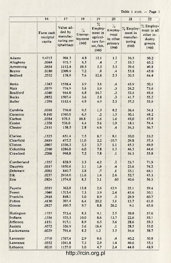
Table 1 cont. — Page 2
16 17 18 19 20 21 22
Farm cash recciptal capita
Value ad-ded by
manufac-turing per inhabitant
/О Unemp-loyment
1960
% Employ-ment in agricul-ture for-est, fish.
1960
/О Employ-
ment in other primary
1960
% Employ-ment in
manufac-turing 1960
% Employ-ment in all other in-
dustry groups
1960
Adams 9.4715 901.3 4.8 12.1 1.2 36.5 50.2 Allegheny .0044 975.7 6.5 .4 .7 33.7 65.2 Armstrong .0654 1112.4 10.3 5.3 5.3 39.6 49.8 Beaver .0180 2309.9 7.2 .8 .4 53.8 45.0 Bedford .2532 178.9 7.6 12.8 2.3 20.5 64.4
Berks .1243 1538.4 3.9 3.6 .4 45.9 50.1 Blair .0579 774.9 5.6 1.9 .3 24.2 73.6 Bradford .4340 964.0 4.8 16.7 .3 33.4 49.6 Bucks .0852 1507.4 3.6 2.8 .3 41.7 55.2 Butler .1296 1163.4 4.9 4.9 2.3 37.2 55.6
Cambria .0318 776.0 9.5 1.3 8.2 36.4 54.1 Cameron 0.190 1760.0 6.5 .2 1.5 50.1 48.2 Carbon .0384 978.5 10.8 1.6 1.6 49,0 47.8 Centre .1358 536.0 4.4 5.6 1.9 18.1 74.4 Chester ,2111 158.5 2.8 6.6 .4 36.3 56.7
Clarion Л525 651.4 7.5 8.7 8.1 30.0 53.2 Clearfield .0419 472.2 11.0 2.2 -10.7 - 29.8 57.3 Clinton .0807 1336.3 5.3 3.7 1.1 45.3 49.9 Columbia .2360 1286.8 6.0 7.8 1.3 46.3 44.6 Crawford .2208 998.8 7.2 7.8 .1 36.3 55.8
Cumberland .1352 828.9 3.3 4.2 .2 23.7 71.9 Dauphin .0517 1050.6 3.1 1.8 .4 23.6 74.2 Delaware .0081 840.7 3.8 .7 .1 35.1 64.1 Elk .0237 2916.0 11.6 1.4 2.6 52.7 43.3 Erie .0824 1574.8 8.5 3.1 .03 40.6 56.3
Fayette .0319 362.8 13.8 2.6 12.9 25.1 59.4 Forest .1046 1313.4 7.3 3.9 2.4 43.6 50.1 Franklin .2818 848.1 5.0 8.9 .5 29.9 60.7 Fulton .4130 207.4 6.4 20.2 3.1 15.7 61.0 Greene .0827 100.5 9.7 8.8 26.2 9.1 65.0
Hutington .1757 573.4 8.3 9.1 2.5 30.8 57.6 Indiana .1334 525.3 10.0 8.6 13.7 22.6 55.1 Jefferson .1151 917.1 8.9 6.5 5.6 28.6 59.3 Juniata .4572 326.9 5.6 16.4 .1 28.5 55.0 Lackawanna .0229 795.6 8.2 1.2 3.5 36.6 58.7
Lancaster .3718 1767.4 2.9 8.6 .4 40.2 50.8 Lawrence .0552 1041.8 7.3 2.9 1.4 40.6 55.1 Lebanon .0210 1127.0 3.0 4.7 2.4 44.0 48.9
http://rcin.org.pl
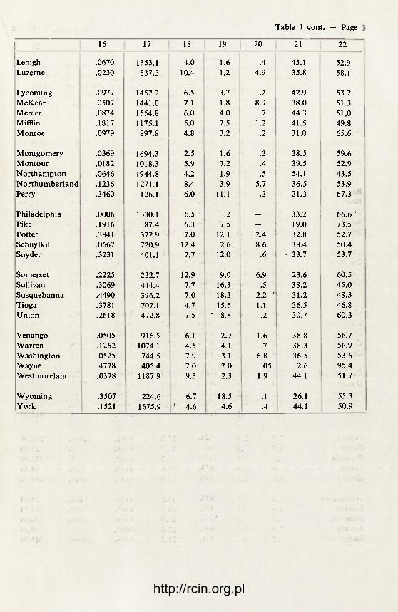
Table 1 cont. — Page 2
16 17 18 19 20 21 22
Lehigh .0670 1353.1 4.0 1.6 .4 45.1 52.9 Luzerne .0230 837.3 10.4 1.2 4.9 35.8 58.1
Lycoming .0977 1452.2 6.5 3.7 .2 42.9 53.2 McKean .0507 1441.0 7.1 1.8 8.9 38.0 51.3 Mercer .0874 1554.8 6.0 4.0 .7 44.3 51,0 Mifflin .1817 1175.1 5.0 7.5 1.2 41.5 49.8 Monroe .0979 897.8 4.8 3.2 .2 31.0 65.6
Montgomery .0369 1694.3 2.5 1.6 .3 38.5 59.6 Montour .0182 1018.3 5.9 7.2 .4 39.5 52.9 Northampton .0646 1944.8 4.2 1.9 .5 54.1 43.5 Northumberland .1236 1271.1 8.4 3.9 5.7 36.5 53.9 Perry .3460 126.1 6.0 11.1 .3 21.3 67.3
Philadelphia .0006 1330.1 6.5 .2 — 33.2 66.6 1
Pike .1916 87.4 6.3 7.5 — 19.0 73.5 Potter .3841 372.9 7.0 12.1 2.4 32.8 52.7 Schuylkill .0667 720.9 12.4 2.6 8.6 38.4 50.4 Snyder .3231 401.1 7.7 12.0 .6 - 33.7 53.7
Somerset .2225 232.7 12.9 9.0 6.9 23.6 60.5 Sullivan .3069 444.4 7.7 16.3 .5 38.2 45.0 Susquehanna .4490 396.2 7.0 18.3 2.2 f 31.2 48.3 Tioga .3781 707.1 4.7 15.6 1.1 36.5 46.8 Union .2618 472.8 7.5 ' 8.8 .2 30.7 60.3
Venango .0505 916.5 6.1 2.9 1.6 38.8 56.7 Warren .1262 1074.1 4.5 4.1 .7 38.3 56.9 Washington .0525 744.5 7.9 3.1 6.8 36.5 53.6 Wayne .4778 405.4 7.0 2.0 .05 2.6 95.4 Westmoreland .0378 1187.9 9.3 ' 2.3 1.9 44.1 51.7
Wyoming .3507 224.6 6.7 18.5 .1 26.1 55.3 York .1521 1675.9 1 4.6 4.6 .4 44.1 50.9
http://rcin.org.pl
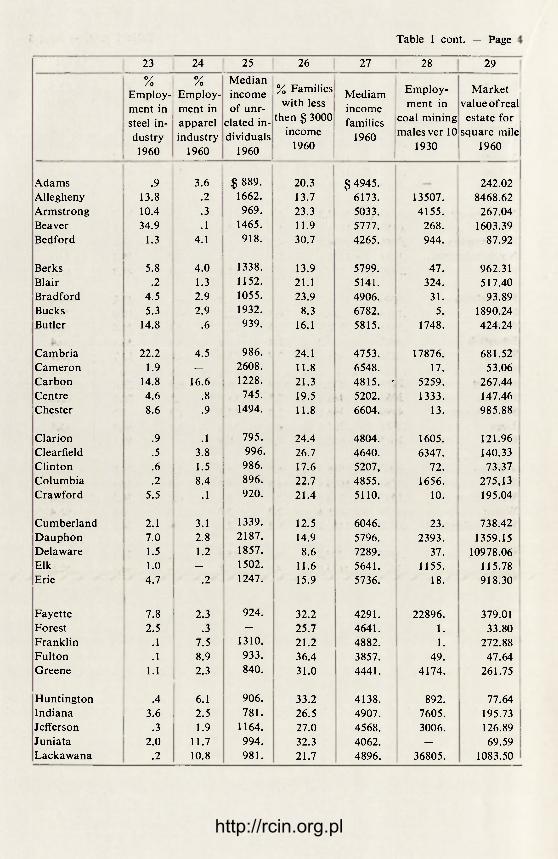
Table 1 cont. — Page 2
23 24 25 26 27 28 29
% Employ-ment in steel in-dustry 1960
% Employ-ment in apparel industry
1960
Median income of unr-
elated in-dividuals
1960
% Families with less
then $ 3000 income
1960
Mediam income families
1960
Employ-ment in
coal mining males ver 10
1930
Market value of real estate for
square mile 1960
Adams .9 3.6 $ 889. 20.3 $ 4945. 242.02 Allegheny 13.8 .2 1662. 13.7 6173. 13507. 8468.62 Armstrong 10.4 .3 969. 23.3 5033. 4155. 267.04 Beaver 34.9 .1 1465. 11.9 5777. 268. 1603.39 Bedford 1.3 4.1 918. 30.7 4265. 944. 87.92
Berks 5.8 4.0 1338. 13.9 5799. 47. 962.31 Blair .2 1.3 1152. 21.1 5141. 324. 517.40 Bradford 4.5 2.9 1055. 23.9 4906. 31. 93.89 Bucks 5.3 2.9 1932. 8.3 6782. 5. 1890.24 Butler 14.8 .6 939. 16.1 5815. 1748. 424.24
Cambria 22.2 4.5 986. 24.1 4753. 17876. 681.52 Cameron 1.9 — 2608. 11.8 6548. 17. 53.06 Carbon 14.8 16.6 1228. 21.3 4815. - 5259. 267.44 Centre 4.6 .8 745. 19.5 5202. 1333. 147.46 Chester 8.6 .9 1494. 11.8 6604. 13. 985.88
Clarion .9 .1 795. 24.4 4804. 1605. 121.96 Clearfield .5 3.8 996. 26.7 4640. 6347. 140.33 Clinton .6 1.5 986. 17.6 5207, 72. 73.37 Columbia .2 8.4 896. 22.7 4855. 1656. 275,13 Crawford 5.5 .1 920. 21.4 5110. 10. 195.04
Cumberland 2.1 3.1 1339. 12.5 6046. 23. 738.42 Dauphon 7.0 2.8 2187. 14.9 5796. 2393. 1359.15 Delaware 1.5 1.2 1857. 8.6 7289. 37. 10978.06 Elk 1.0 — 1502. 11.6 5641. 1155. 115.78 Erie 4.7 .2 1247. 15.9 5736. 18. 918.30
Fayette 7.8 2.3 924. 32.2 4291. 22896. 379.01 Forest 2.5 .3 — 25.7 4641. 1. 33.80 Franklin .1 7.5 1310. 21.2 4882. 1. 272.88 Fulton .1 8.9 933. 36.4 3857. 49. 47.64 Greene 1.1 2.3 840. 31.0 4441. 4174. 261.75
Huntington .4 6.1 906. 33.2 4138. 892. 77.64 Indiana 3.6 2.5 781. 26.5 4907. 7605. 195.73 Jefferson .3 1.9 1164. 27.0 4568. 3006. 126.89 Juniata 2.0 11.7 994. 32.3 4062. — 69.59 Lackawana .2 10.8 981. 21.7 4896. 36805. 1083.50
http://rcin.org.pl

Table 1 cont. — Page 2
23 24 25 | 26 27 28 29
Lancaster 1.6 4.9 1554. 14.9 5810. 3. 963.08 Lawrence 11.2 .2 991. 15.9 5617. 344. 897.75 Lebanon 10.1 7.9 1547. 14.1 5512. 103. 695,52 Lehigh 8.6 8.1 1528. 12.4 6064. 22. 2128.10 Luzerne .7 12.3 1012. 24.8 4722. 63770. 780.98
Lycoming 3.6 5.1 1417. 19.0 5235. 56. 230.45 McKean .1 _ 1559. 17.2 5299. 3. 173.08 Mercer 16.8 .1 953. 15.6 5872. 254. 591.99 Mifflin 9.0 4.9 1224. 22.8 4860. — 223.32 Monroe 2.2 4.1 1268. 20.3 5093. 11. 248.61
Montgomery 3.5 2.6 1877. 7.4 7632. 49. 4835.07 Montour .7 4.2 838. 20.5 5134. 9. 237.73 Northampton 16.1 11.8 1240. 14.2 5709. 23. 2055.29 Northumberland 1.6 12.4 1118. 27.5 4544. 12971. 414.45 Perry 2.6 5.3 1045. 25.8 4725. 17. 84.14
Philadelphia .9 4.7 1863. 17.1 5782. 192. 45512.30 Pike .4 3.2 1169. 24.1 4872. 4. 113.71 Potter — .7 996. 26.8 4547. 3. 26.48 Schuylkill 3.7 16.7 1088. 26.4 4605. 36060. 373.16 Synder 1.8 9.2 824. 25.6 4648. 20. 124.66
Somerset 5.3 6.8 903. 33.3 4055. 9764. 140.75 Sullivan .5 8.0 1222. 28.4 4322. 506. 27.01 Susquehanna 2.0 3.3 884. 25.8 4815. 1127. 63.70 Tioga 1.9 — 888. 23.3 4775. 559. 55.70 Union 2.2 2,3 775. 22.5 5032. 2. 155.88
Venango 3.7 1307. 18.7 5307. 89. 213.34 Warren 6.7 .1 1635. 15.5 5756. 5. 123.61 Washington 17.7 .2 1178. 19.4 5386. 17832. 651.68 Wayne 1.1 969. 28.1 4444. 284. 95.78 Westmoreland 16.0 .4 1134. 17.7 5597. 17210. 1051.50
Wyoming 5.6 953. 30.1 4247. 83. 97.13 York 1.0 4.9 1653. 15.2 3676. 22. 759.22
http://rcin.org.pl

30 31 32 33 34 35 36 Net Median Employ-
Popula- migra- farm % Unem- ment % Urba- Expendi-tion tion income ployment manufac- nized tures 1960 1950-
- 1 9 6 0 1960 1960 turing
1960 1960 pupil 1960
Popula-tion 1950
Popula-tion 1950
Median farm
income 1950
% Unem-ployment
1950
Employ-ment ma-nufactu-ring 1950
% Urba-nized 1950
Expen-ditures
pupil 1950
Adams 1.17 + .02 1.95 1.66 1.16 .95 1.69 Allegheny 1.07 - . 0 6 1.79 1.10 .96 1.03 1.73 Armstrong .98 - . 1 5 1.75 1.51 .97 .82 1.44 Beaver 1.18 + .01 1.70 1.67 1.03 .97 1.43 Bedford 1.04 - . 1 0 2.27 1.15 1.25 1.01 1.48
Berks 1.08 + .01 1.71 1.44 .98 .97 1.45 Blair .98 - . 1 1 1.86 1.19 1.57 .95 1.45 Bradford 1.06 - . 0 6 1.95 .91 1.42 .97 1.62 Bucks 2.13 + .81 1.96 1.44 1.86 2.01 1.45 Butler 1.17 + .02 1.98 .74 1.43 .89 1.67
Cambria .97 - . 1 7 1.65 1.38 1.12 .99 1.43 Cameron 1.08 - . 1 0 2.01 1.71 .87 .86 1.14 Carbon .92 - . 1 5 1.62 1.35 1.24 .96 1.36 Centre 1.19 + .03 1.99 .79 1.33 1.01 1.67 Chester 1.32 + .17 2.01 .97 1.40 1.05 1.52
Clarion .98 - . 1 5 1.93 1.25 1.82 1.16 1.59 Clearfield .95 - . 1 6 1.91 1.57 1.20 1.01 1.40 Clinton 1.03 - . 0 9 1.97 .95 1.13 .97 1.39 Columbia 1.00 - . 0 9 1.81 ' .71 1.24 .98 1.56 Crawford .99 - . 1 2 1.77 1.13 1.07 .91 1.45
Cumberland 1.32 + .16 1.89 1.57 1.34 1.02 1.60 Dauphin 1.11 - . 0 1 1.76 1.11 1.05 .99 1.42 Delaware 1.34 + .15 1.76 .75 1.25 1.07 1.36 Elk 1.08 - . 0 8 1.85 3.63 .88 .96 1.42 Erie 1.14 - . 0 3 1.69 2.07 .88 1.01 1.37
Fayette .89 - . 2 1 1.56 1.57 1.14 .98 1.42 Forest .91 - . 1 6 1.96 .96 1.17 — 1.45 Franklin 1.16 + .01 1.82 1.43 1.22 .90 1.58 Fulton 1.02 - . 1 1 2.39 1.78 1.29 — 1.85 Greene .87 - . 2 3 1.69 1.59 1.54 1.09 1.34
Huntington .97 - . 1 4 1.77 1.32 1.08 .98 1.69 Indiana .98 - . 1 4 1.96 1.28 1.84 .95 1.53 Jefferson .95 - . 1 5 1.87 1.25 1.04 1.03 1.76 Juniata 1.04 - . 0 9 1.96 1.81 1.12 — 1.48 Lackawanna .91 - . 1 5 1.74 1.21 1.14 .98 3.03
http://rcin.org.pl
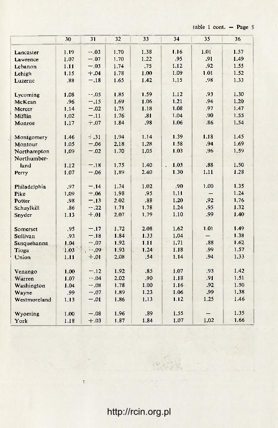
Table 1 cont. — Page 2
30 31 32 33 34 35 36
Lancaster 1.19 - . 0 3 1.70 1.38 1.16 1.01 1.57 Lawrence 1.07 - . 0 7 1.70 1.22 .95 .91 1.49 Lebanon 1.11 - . 0 3 1.74 .75 1.12 .92 1.55 Lehigh 1.15 + .04 1.78 1.00 1.09 1.01 1.52 Luzerne .88 - . 1 8 1.65 1.42 1.15 .98 1.33
Lycoming 1.08 - . 0 5 1.85 1.59 1.12 .93 1.30 McKean .96 - . 1 5 1.69 1.06 1.21 .94 1.20 Mercer 1.14 - . 0 2 1.75 1.18 1.08 .97 1.47
! Mifflin 1.02 - . 1 1 1.76 .81 1.04 .90 1.55 Monroe 1.17 + .07 1.84 .98 1.06 .86 1.54
Montgomery 1.46 + .31 1.94 1.14 1.39 1.18 1.45 Montour 1.05 - . 0 6 2.18 1.28 1.58 .94 1.69 Northampton 1.09 - . 0 2 1.70 1.05 1.03 .96 1.59 Northumber-
land 1.12 - . 1 8 1.75 1.40 , 1.03 .88 1.50 Perry 1.07 - . 0 6 1.89 2.40 1.30 1.11 1.28
Philadelphia .97 - . 1 4 1.74 1.02 .90 1.00 1.35 Pike 1.09 + .06 1.98 .95 1.11 — 1.24 Potter .98 - . 1 3 2.02 .88 1.20 .92 1.76 Schuylkill .86 - . 2 2 1.71 1.78 1.24 .95 1.32 Snyder 1.13 + .01 2.07 1.79 1.10 .99 1.40
Somerset .95 - . 1 7 1.72 2.08 1.62 1.01 1.49 Sullivan .93 - . 1 8 1.84 1.33 1.04 - 1.38 Susquehanna 1.04 - . 0 7 1.92 1.11 1.71 .88 1.62 Tioga 1.03 . - . 0 9 1.93 1.24 1.18 .99 1.57
1 Union 1.11 + .01 2.08 .54 1.14 .94 1.33
Venango 1.00 - . 1 2 1.92 .85 1.07 .93 1.42 Warren 1.07 - . 0 4 2.02 .90 1.18 .91 1.51 Washington 1.04 - . 0 8 1.78 1.00 1.16 .92 1.50 Wayne .99 - . 0 7 1.89 1.23 1.06 .99 1.38 Westmoreland 1.13 - . 0 1 1.86 1.13 1.12 1.25 1.46
Wyoming 1.00 - . 0 8 1.96 .89 1.55 — 1.35 York 1.18 + .03 1.87 1.84 1.07 1.02 1.66
r
http://rcin.org.pl
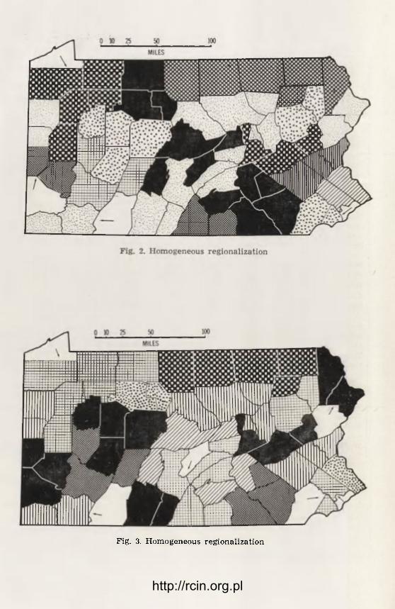
Fig. 3. H o m o g e n e o u s r eg iona l i za t i on
http://rcin.org.pl
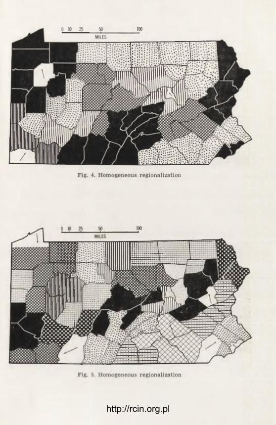
http://rcin.org.pl

Fig. 6. Homogeneous regionalization
Fig. 3. Homogeneous reg iona l iza t ion
http://rcin.org.pl

REGION A L I Z A T I O N OF P E N N S Y L V A N I A COUNTIES 177
Table 2
No. of Factors Characterization of factors
Map name
Factors used
2 1. Urban A (1, 2) 2. Rural
3 1. Manufacturing decline B (1, 2, 3) 2. Rural poverty —"Appalachian" 3. Urbanized stagnation
4 1. Surburbanism C (1, 2, 3, 4) 2. Urban poverty —"Appalachian" 3. Urban stagnation 4. Urban-manufacturing decline
5 1. Heavy industrialization D (1, 3, 5) 2. Urban poverty— "Appalachian" 3. Urban stagnation 4. Suburbanism 5. Rural poverty —"Appalachian"
6 1. Urban manufacturing decline E (1, 3, 5, 6) 2. Rural poverty— "Appalachian" 3. Urban stability 4. Relative growth 5. Heavy industrialization 6. Urban poverty— "Appalachian"
7 1. Suburbanism F (1, 2, 3, 5, 7) 2. Urban-manufacturing decline 3. Urban stability 4. Relative growth 5. Heavy industrialization 6. Urban poverty— "Appalachian" 7. Rural poverty —"Appalachian"
The step-by-step regionalization procedure for each map is given in the attached IBM printout with a code letter which keys to the map and to Table 2. The resulting regionalization maps are relatively self-explana-tory. Note that in every case excessively large regions have been avoided by picking the step which seemed to give the best balance of size and number of regions. The result has been, in every case, a number of one--county left-over regions. These are not colored on the maps, but in each case an arrow is drawn indicating the region to which the county should probably be attached. Notice also that there are a number of cases where counties in the same region are coniguous only at their corners. This is unfortunately unavoidable with the regionalization procedure used, although it is not clear how much difference it really makes.
One small point is worth noting in passing. The recently formed "Nor-thern Tier Regional Planning Commission", which includes Tioga, Brad-ford, Susquehanna, Wyoming, and Sullivan counties, shows up fairly well
12 G e o g r a p h i a P o l o n i c a t . 15 http://rcin.org.pl

178 BENJAMIN H. STEVENS A N D C A R O L Y N A . B R A C K E T T
in several of the regionalizations. In some cases Sullivan and/or Wyoming appear as a group. It is interesting, however, that Potter usually appears with them although it was not included in the Regional Planning Com-mission.
N O D A L R E G I O N A L I Z A T I O N
As already suggested, handicraft methods were used for the nodal regionalization of Pennsylvania counties, mainly because adequate lin-kage data were unavailable. Attempts to obtain phone-call, travel, sales, and other data proved unsuccessful. Therefore the regionalization had to be based on a combination of newspaper circulation data, a gravity model formulation to delimit market areas, and subjective judgment.
Fig. 8. Nodal regionalization S o u r c e s : N e w s p a p e r c i r c u l a t i o n f r o m " C i r c u l a t i o n 64", A m e r i c a n N e w s p a p e r M a r k e t s , I n c . ; p o p u l a t i o n f r o m t h e U . S . C e n s u s of P o p u l a t i o n ; d i s t a n c e s f r o m R a n d M c N a l l y R o a d A t l a s
The gravity model used is a simple form of the more general gravity and potential concepts described in Carrothers (1956). The influence of a node i on a point j is assumed to be:
http://rcin.org.pl

R E G I O N A L I Z A T I O N OF P E N N S Y L V A N I A C O U N T I E S 179
where Pi is the population of the node and da is the airline distance from i to j. A point j is assumed to be tr ibutary to the node which has the greatest influence upon it.
Unfortunately, counties are usually not nodes themselves but rather contain nodes. Therefore the location of the node in a county should affect the influence of the county on its neighbors. Similarly, the popu-lation of potential t r ibutary counties is not evenly distributed. Thus a county with a strong node near its eastern boundary, for example, may dominate the county to its east, especially if the population of that county is concentred in its western portion. But the western population of the nodal county may, in turn, be t r ibutary to a node in another county.
One possible conclusion is that except for counties which are small enough, are generally urbanized, and have a major center city, most counties are too large in size to be effective units for nodal regionalizat-ion. In any case, it can be very misleading to use total county population for P.-. And distance between geographic county centroids may not be the best measure for da. In fact, such a formulation is clearly useless in determining whether a county is tr ibutary to a node contained within it.
A suggested alternative is to use the population of the largest urban area in the county for Pi and the distance between the center of this urban area and the center of gravity of all population in a potential tr i-butary county as da. Obviously, one tr ibutary population could be within the county containing the node.
It is not clear that this method would avoid all the problems outlined above or that it might not lead to pairs of counties which were mutually dominant. A county containing two large nodes would clearly present difficulties. Further experimentation will be necessary before satisfactory nodal regionalizations of counties can be produced by this method. And, in any case, no gravity formulation is likely to be a substitute for good linkage data.
The only recent linkage data available for Pennsylvania concerns newspaper circulation by county. But there could easily be a worse set of data for regionalization purposes. For each county it is immediately possible to determine whether the dominant circulation is of a newspaper within the county. If it is not. the county is not likely to be nodal, and the problem is thereby simplified.
Since the data is based on total circulations within the county, the problems of determining the center of gravity of population and distances from nodes to tr ibutary populations does not arise. The node which publishes the dominant newspaper in the county is likely to be the node to which the county is tr ibutary.
However, it is still possible to be misled. If the ratio of the biggest
is* http://rcin.org.pl

B E N J A M I N H. S T E V E N S A N D C A R O L Y N A . B R A C K E T T
Table 3 Newspaper circulation for Pennsylvania counties
County County source of largest circulation
% House-holds
covered
County source of 2nd largest circula-
tion
% House-holds cov.
Adams Adams 47 York 39 Allegheny Allegheny 92 Allegheny 7 Armstrong Armstrong 43 Westmoreland 20 Beaver Beaver 48 Beaver 31 Bedford Cambria 10 Huntington 7 Berks Berks 95 Lehigh 3 Blair Blair 77 Blair 7 Bradford Bradford 37 Bradford 32 Bucks Bucks 41 Philadelphia 31 Butler Butler 68 Allegheny 24 Cambria Cambria 74 Allegheny 4 Cameron McKean 33 Erie (New York) 14 Carbon Lehigh 53 Luzerne 11 Centre Philadelphia 11 Allegheny 5 Chester Philadelphia 29 Philadelphia 29 Clarion Venango 33 Allegheny 20 Clearfield Clearfield 25 Allegheny 9 Clinton Clinton 76 Philadelphia 8 Columbia Columbia 28 Philadelphia 6 Crawford Crawford 62 Mahoning 20 Cumberland Dauphin 74 Cumberland 25 Dauphin Dauphin 98 Philadelphia 1 Delaware Philadelphia 51 Philadelphia 34 Elk Allegheny 11 Erie 7 Erie Erie 93 Crawford 1 Fayete Fayette 48 Fayette 17 Forest Venango 44 Allegheny 9 Franklin Allegheny (Maryland) 44 Franklin 29 Fulton Huntington 9 Franklin 6 Greene Washington 27 Allegheny 15 Huntingdon Huntingdon 75 Philadelphia 6 Indiana Indiana 57 Allegheny 15 Jefferson Allegheny 22 Clearfield 18 Juniata Mifflin 34 Dauphin 24 Lackawanna Lackawanna 74 Lackawanna 41 Lancaster Lancaster 95 Philadelphia 5 Lawrence Lawrence 67 Allegheny 16 Lebanon Lebanon 83 Philadelphia 9 Lehigh Lehigh 97 Berks 49 Luzerne Berks 90 Luzerne 70 Lycoming Lycoming 81 Philadelphia 3 McKean McKean 58 Cattaraugus (N. Y.) 10 Mercer Mercer 56 Mercer 15
http://rcin.org.pl

REGION A L I Z A T I O N OF P E N N S Y L V A N I A COUNTIES 63
T a b l e 3, cont.
County County source of largest circulation
% House-holds
covered
County source of 2nd largest circula-
tion
% House-holds cov.
Mifflin Mifflin 82 Philadelphia 7 Monroe Monroe 70 N. Y. C. 12 Montgomery Philadelphia 45 Philadelphia 36 Montour Northumberland 16 Philadelphia 12 Northampton Northampton 44 Northampton 33 Northumberland Northumberland 32 Northumberland 32 Perry Dauphin 63 Philadelphia 3 Philadelphia Philadelphia 64 Philadelphia 44 Pike Orange (N. Y.) 31 N. Y. C. 22 Potter Cattarargus (N. Y.) 25 Chemong (N. Y.) 14 Schuykill Schuykill 52 Philadelphia 14 Snyder Northumberland 66 Mifflin 6 Somerset Cambria 40 Somerset 23 Sullivan Sullivan 28 Lycoming 16 Susquehanna Broome 26 Susquehanna 14 Tioga Chemung (N. Y.) 57 Philadelphia 19 * Union Northumberland 63 Philadelphia 8 Venango Venango 84 Allegheny 5 Warren Warren 65 Warren 45 Washington Allegheny 39 Washington 31 Wayne Lackawanna 34 Lackawanna 18 Westmoreland Allegheny 35 Westmoreland 17 Wyoming Lackawanna 26 Luzerne 21 York York 49 j York 46 „
Note: The percentages may add to more than 100%, because some households take more than one newspapei . Source: „Circulat ion 64", American Newspaper Markets , Inc. , Northfield, Illinois.
circulation to the next biggest is not very high, the difference might be due merely to the relative qualities of the newspapers. An equalization of quality could then shift the dominance to what at first appears to be the secondary node. Furthermore, there is obviously a difference in the influence, as well as the content, of daily and weekly newspapers. Subjec-tive judgments are still necessary and a f i rm knowledge of the areas being regionalized can certainly help.
The results of the nodal regionalization are presented in Fig. 9. The data on newspaper circulation appears in Table 3, but the gravity meas-ures were omitted because they were so unsatisfactory. With more extensive linkage data, the results could probably be improved. Never-theless, this first at tempt at nodal regionalization of Pennsylvania had some intuitive appeal.
The most significant feature of the nodal regionalization is the dif-
http://rcin.org.pl
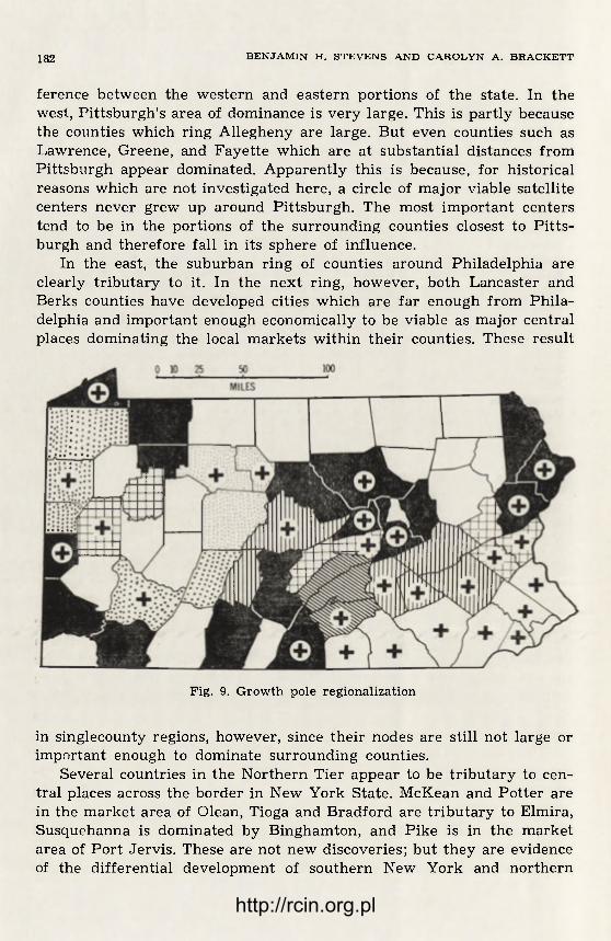
182 B E N J A M I N H. S T E V E N S A N D C A R O L Y N A . B R A C K E T T
ference between the western and eastern portions of the state. In the west, Pittsburgh's area of dominance is very large. This is partly because the counties which ring Allegheny are large. But even counties such as Lawrence, Greene, and Fayette which are at substantial distances f rom Pittsburgh appear dominated. Apparently this is because, for historical reasons which are not investigated here, a circle of major viable satellite centers never grew up around Pittsburgh. The most important centers tend to be in the portions of the surrounding counties closest to Pit ts-burgh and therefore fall in its sphere of influence.
In the east, the suburban ring of counties around Philadelphia are clearly tr ibutary to it. In the next ring, however, both Lancaster and Berks counties have developed cities which are far enough from Phila-delphia and important enough economically to be viable as major central places dominating the local markets within their counties. These result
Fig. 9. Growth pole regionalization
in singlecounty regions, however, since their nodes are still not large or important enough to dominate surrounding counties.
Several countries in the Northern Tier appear to be tr ibutary to cen-tral places across the border in New York State. McKean and Potter are in the market area of Olean, Tioga and Bradford are t r ibutary to Elmira, Susquehanna is dominated by Binghamton, and Pike is in the market area of Port Jervis. These are not new discoveries; but they are evidence of the differential development of southern New York and northern
http://rcin.org.pl

R E G I O N A L I Z A T I O N OF P E N N S Y L V A N I A COUNTIES 183
Pennsylvania. Similarly, Fulton and Franklin counties are tr ibutary to Hagerstown, Maryland and Mercer county is in the market area of Youngstown, Ohio. One minor surprise here is that Greene county is t r ibutary to Pit tsburgh rather than to Wheeling, West Virginia. Wheeling apparently is too small and too far away to overcome the dominating effects of Allegheny county.
G R O W T H P O L E R E G I O N A L I Z A T I O N
An experimental growth pole regionalization for Pennsylvania was tried employing the linear programming technique described above and in Appendix 1. Although it had been hoped to use the scores of counties on the "growth" factors noted in several of the factor analyses in Table 2, this was not possible. The factor analysis technique, as used for the ho-mogeneous regionalization, does not automatically print out the scores of counties on factors. A special program would have had to be writ ten to extract these scores. Therefore, for experimental purposes, it was decided that population growth would suffice.
The measurement used was the standard score of the population growth of each county; i. e. the number of standard deviations above or below the mean per cent growth for all counties. Counties with positive scores were defined as growth absorbers.
The objective of the regionalization was to link declining to growing counties in such a way as to maximize the internal homogeneity of the resulting regions. Despite the questions raised in this report about the merits of this objective, it was decided to employ it in this experiment. Furthermore, it was assumed that the higher the standard score, the more growth-inducing potential a county would have, and vice versa. Therefore a high-score county could "afford" to have attached to it a relatively larger number of negative-score counties as long as the total score of the resulting region did not become negative. This too is a questionable procedure.
Difficulties were encountered even before the application of the method. The rapidly-growing counties in the southeast are completely surrounded by a ring of counties which are also growing. Much of the inner ring of counties is part the Philadelphia Metropolitan Area which is a growth pole region even though the city of Philadelphia is not itself growing. It was decided, therefore, to leave these counties (Adams, York, Lancaster, Chester, Delaware, Montgomery, and Bucks) out of the analysis.
This decision created a dearth of growth poles relative to growth ab-sorbers. But it can be argued that this is reasonable since the heavy con-
http://rcin.org.pl

184 B E N J A M I N H. S T E V E N S A N D C A R O L Y N A . B R A C K E T T
centration of growing counties in the southeast should logically make it difficult to form growth pole regions in less fortunate parts of the state.
The results, displayed in Fig. 9, indicate the effects of the regional imbalance within the state. The whole northern tier, the hard coal area, the petroleum-producing region, and parts of the soft coal area all lacked nearby growth poles strong enough to regionalize upon. Certain isolated counties such as Montuor, Fulton, Greene, and Somerset were also left out in the regionalization. This was due to the non-homogeneity of these counties relative to their surrounding growth pole regions and to the lack of growth potential in the nearby growth poles. These results, and the shape of the regions in general, would have been different if com-pactness had been part of the objective.
Notice that several regions contain two or more contignous growth poles. This resulted from the assumption that a combination of modera-tely weak poles might be strong enough to generate growth in a declin-ing area where a single weak pole would not suffice.
Finally, one fur ther problem needs to be noted. A comparison of the nodal and growth pole regionalizations reveals the possible dangers of failing to recognize linkages in the growth pole technique. Cumberland county, for example, is growing because of the growth of Harrisburg in Dauphin county to which it is strongly linked. It is reasonable to question whether Cumberland county should, in turn, be considered a growth pole for Per ry and Juniata counties, especially since both of the latter are also tributaries of the Dauphin county node.
In general, then, the experiment cannot be considered an unqualified success. Some of the deficiencies are easily correctable; others are not. Both definitional and methodological questions will have to be answered before a definitive technique can be developed.
CONCLUSIONS
Throughout this report questions have been raised which clearly re-quire fu r ther study. To recapitulate the more important problems, they include: 1) identification and measurement of growth and growth poles; 2) improvement of growth pole regionalization techniques; 3) measure-ment of the effects of linkage on the diffusion of growth; 4) development of better surrogates for unavailable linkage data; 5) evaluation of the relative merits of homogeneity, linkage, and growth as criteria for re-gionalization for economic development planning purposes; test of the effects of allowing regions to cross state boundaries; and 7) experimen-tation with weighted cominations of criteria.
http://rcin.org.pl

R E G I O N A L I Z A T I O N OF P E N N S Y L V A N I A COUNTIES 185
Some testing and experimentation are already being done in con-nection with a second study covering the states of Wisconsin, Minnesota, and Michigan. However, research on the basic questions of regional economic growth must await fur ther studies designed specifically for this purpose. Without the results of such research, and failing the ans-wers tq these basic questions, the formation of regions for economic development planning purposes will have to depend upon criteria and techniques of questionable utility.
APPENDIX l
E X P E R I M E N T A L L I N E A R P R O G R A M M I N G T E C H N I Q U E F O R G R O W T H P O L E R E G I O N A L I Z A T I O N
Given: n counties to be regionalized of which counties (1, 2, . . . , m) are growth poles or "sources" of growth and counties (m+1, m + 2 , n) are declining counties or "sinks" of growth.
Let: Tjj be a variable which takes a non-zero value only when counties i and j are placed together in the same region. gt be the "growth potential" of county i, (¿=1, 2, . . . , m) Sj be the "growth absorption capacity" of county j, (j=m +1, m+2, . . . , n) djj be tre "distance", measured in squared differences of scores on the factors of the homogeneous factor analysis of counties i and j, (i, j— 1, 2 n)
Minimize:
i LdijTij (1) i=U=i
Subject to: n
- ^ T ^ - g i ( i = l , 2 , . . . ,m) (2a) j = m+ 1
n m Z ( T v - T j J + X T ^ s j ( j = m + I , m + 2 , . . . , n) (2b) h = m+X i— I
T i ^ O for all i, j. lJ | = 0 where conties i and j are noncontiguous.
Note: The first term of (2b) allows for the "transshipments" of growth from any "sink" county to any other. This permits a "source" county to be linked to a "sink" county to which it is not contiguous if the growth potential is large enough to satisfy both the contiguous and the non-contiguous county. No direct interpretation is given to the sizes of the In this experiment only the existence of nonexistence of regional l in-kage is considered. By the same token, the dual variables are not in-terpreted. Therefore the dual linear programming problem is not presented here.
http://rcin.org.pl

186 BENJAMIN H. STEVENS A N D C A R O L Y N A . B R A C K E T T
APPENDIX 2
Given: Let:
Objective:
Where:
Remarks:
C O M B I N A T I O N O F T E C H N I Q U E S F O R R E G I O N A L I Z A T I O N
n counties to be regionalized. Gs
h be the set of counties, to be determined, contained in region h at step s of the regionalization procedure. A county i (i—1, 2, . . . , to) belongs, at any step s, to at least one but only one of such regions. This means that there may be several single-county regions at any parti-cular step. ms
h be the number of counties contained in region h at step s. In particular m — 1 for all h since each must be in a region by itself before the procedure starts. djj be the sum of the squares of the differences on the socioeconomic factor scores of counties i and j (homogeneity criterion). ejj be the "strength" of the linkage between counties i and j (nodality criterion). fjj be the square of airline (or other geographic) distance measure from the centroid of county i to the centroid of county j (compactness cri-terion). A, B, C be the weighting or relative importance given to homogeneity, nodality, and compactness respectively. During step s + 1 form that combination of set GyJs
g and GyJsh for which
(1)
(2a)
(2b)
The calculations in (2a) and (2b) are simply to compute the "dif-ferences" between all possible pairs of regions. The presumption is that the "difference" between any two regions on any one of the three criteria is the mean of the "differences" between one of the regions and each of the counties in the other on that criterion. At each step, the procedure joins two previously-formed regions, one or both of which may be singlecounty regions. If h is a single-county region, the calcu-lation of (2b) becomes immediate; if g is single-county, (2a) is im-mediate; if both are single-county, both calculations are unnecessary since the x g
sh are merely the corresponding given diy-, or ftj.
The procedure, if allowed to run enough steps, will eventually group all counties into a single region. Therefore, an arbitrary cutoff point has to be selected where the regionalization appears "satisfactory". With the exception of the addition of two criteria and the relative weighting of criteria this combination of techniques is very similar to the ho-mogeneous regionalization technique of Berry. In fact, the procedure will produce a strictly homogeneous regionalization if A, B, and C are set equal to 1, 0, and 0 respectively. Similarly, a strictly nodal regio-
http://rcin.org.pl
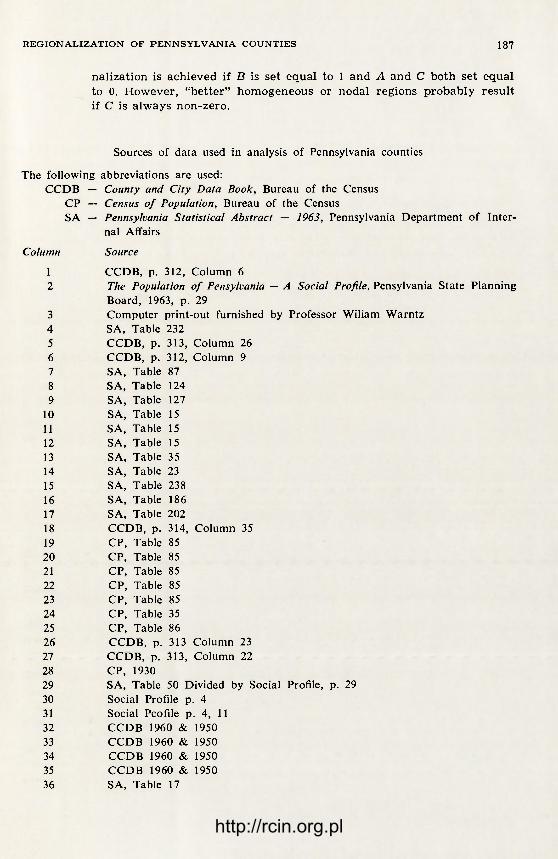
R E G I O N A L I Z A T I O N OF P E N N S Y L V A N I A C O U N T I E S 187
nalization is achieved if B is set equal to 1 and A and C both set equal to 0. However, "better" homogeneous or nodal regions probably result if C is always non-zero.
Sources of data used in analysis of Pennsylvania counties
The following abbreviations are used: CCDB — County and City Data Book, Bureau of the Census
CP — Census of Population, Bureau of the Census SA — Pennsylvania Statistical Abstract — 1963, Pennsylvania Department of Inter-
nal Affairs
Column Source
1 CCDB, p. 312, Column 6 2 The Population of Pensylvania — A Social Profile, Pensylvania State Planning
Board, 1963, p. 29 3 Computer print-out furnished by Professor Wiliam Warntz 4 SA, Table 232 5 CCDB, p. 313, Column 26 6 CCDB, p. 312, Column 9 7 SA, Table 87 8 SA, Table 124 9 SA, Table 127
10 SA, Table 15 11 SA, Table 15 12 SA, Table 15 13 SA, Table 35 14 SA, Table 23 15 SA, Table 238 16 SA, Table 186 17 SA, Table 202 18 CCDB, p. 314, Column 35 19 CP, Table 85 20 CP, Table 85 21 CP, Table 85 22 CP, Table 85 23 CP, Table 85 24 CP, Table 35 25 CP, Table 86 26 CCDB, p. 313 Column 23 27 CCDB, p. 313, Column 22 28 CP, 1930 29 SA, Table 50 Divided by Social Profile, p. 29 30 Social Profile p. 4 31 Social Pcofile p. 4, 11 32 CCDB 1960 & 1950 33 CCDB 1960 & 1950 34 CCDB 1960 & 1950 35 CCDB 1960 & 1950 36 SA, Table 17
http://rcin.org.pl

http://rcin.org.pl

G E O G R A P H I A P O L O N I C A 15
T A X O N O M I C M E T H O D S I N R E G I O N A L S T U D I E S
STANISŁAW L E W I Ń S K I
For several recent years, we have been witnessing an increasing application of taxonomic methods in regionalization. In particular, the method of factor analysis and the "linkage tree" method described by B. J. L. Berry are well known 1.
This paper describes the Polish taxonomic method called the "Wro-claw taxonomy". It seems that this method has several advantages in comparison to the linkage tree method, such as, e.g., the simplicity and inexpensiveness of the calculations and the suggestiveness of the picture obtained, and it deserves to be presented to a wider public.
H I S T O R Y OF TAXONOMY IN POLAND
Studies in taxonomic method as well as attempts at the practical application of them have a fairly long and rich history in Poland. They developed out of the co-operation between the mathematicians assemb-led around Professor H. Steinhaus and a group of autstanding anthro-pologists, naturalists and geographers.
The first paper by a Polish author containing an example of the taxonomic method was ,T. Czekanowski's article writ ten in 1909 2. This method was improved in the period between the World Wars 3. Its author studied sets of points, each of which was characterized by a definite number of features. On the assumption that the units of the population
1 B. J. L. Berry, The mathematics of economic regionalization, Economic Re-gionalization (ed. M. Mackes), Prague, 1967.
2 J. Czekanowski, Zur Differenzialdiagnose der Neandertalgruppe, Korres-pondenzblatt d.D.G.F. Anthr. u. Urgesch, 11, Jahrg. No. 6/7, Braunschweig, 1909.
3 J. Czekanowski, Metoda podobieństwa w zastosowaniu do badań psycho-metrycznych, Lwów, 1926.
http://rcin.org.pl
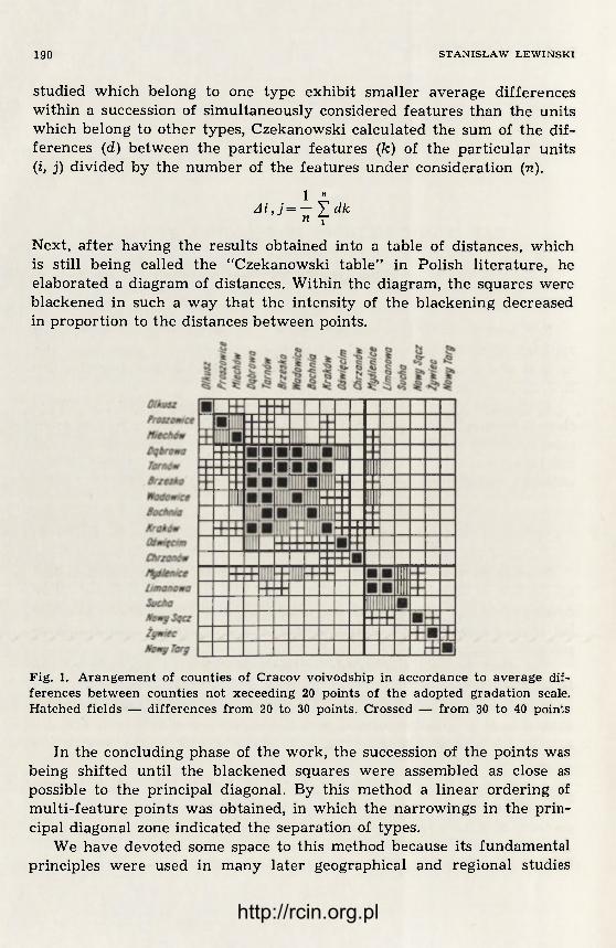
190 S T A N I S L A W L E W I Ń S K I
studied which belong to one type exhibit smaller average differences within a succession of simultaneously considered features than the units which belong to other types, Czekanowski calculated the sum of the dif-ferences (d) between the particular features (k) of the particular units (i, j) divided by the number of the features under consideration (n).
1 « Ai, j = — Y dk
n f
Next, af ter having the results obtained into a table of distances, which is still being called the "Czekanowski table" in Polish literature, he elaborated a diagram of distances. Within the diagram, the squares were blackened in such a way that the intensity of the blackening decreased in proportion to the distances between points.
Fig. 1. Arangement of counties of Cracov voivodship in accordance to average dif-ferences between counties not xeceeding 20 points of the adopted gradation scale. Hatched fields — differences from 20 to 30 points. Crossed — from 30 to 40 points
In the concluding phase of the work, the succession of the points was being shifted until the blackened squares were assembled as close as possible to the principal diagonal. By this method a linear ordering of multi-feature points was obtained, in which the narrowings in the prin-cipal diagonal zone indicated the separation of types.
We have devoted some space to this method because its fundamental principles were used in many later geographical and regional studies
http://rcin.org.pl
T A X O N O M I C M E T H O D S 191
(J. Fierich, Z. Wysocki, M. Najgrakowski, A. F a j f e r e k t h e diagram (Fig. 1) which is intended to serve as an example of the method has been borrowed from J. Fierich's study).
The method of diagrams, however, has essential déficiences. It is im-precise. Shifting in the diagrams is carried out by way of trials. There is no certainty whether the selected arrangement is really the best. Doubts have also been evoked by the very principle of ordering a multi--feature set along a single dimension or line.
THE WROCLAW TAXONOMY
Having in mind these limitations, a group of mathematicians f rom Wroclaw put forward a new method called the "Wroclaw taxonomy" or the "Wroclaw dendrite" 5.
Like the previous methods, the Wroclaw taxonomy deals with the analysis of large populations in which each individual is characterized by a large number of measurable features. All individuals in the popu-lation are interpreted as points in a multidimensional space, and the features as coordinates of the points. Such a set of points, characterized by a certain number of features, is called a set of individual points.
The Wroclaw taxonomy method makes possible the examination of the internal structure of a set of individual points. This is effected by (1) joining the neighbouring individual points into groups; (2) finding the points or areas characteristic of the given set of individual point; (3) dividing the set into parts; (4) connecting the points of the set by an ordering line.
The application of the method will be exemplified by a study of ty-pes of towns in Poland which was carried out in the Institute of Town Planning and Architecture in Warsaw.
4 J. Fierich, Próba zastosowania metod taksonomicznych do rejonizacji sy-stemów rolnych w województwie krakowskim (An Attempt of Application of Taxonomic Methods to the Regionalization of Agricultural Systems in Voivodship of Cracov). Myśl gospodarcza, 1, Kraków, 1957, pp. 73—100; Najgrakowski, M., Re-gionalization of Dispersed on the Example of Polish Building Ceramics Industry, Przegląd Geograficzny, 35, 1963, pp. 31—50; Zb. Wysocki, The Frequency of the Economico-geographical Groups or Features Using the Example of Poland, Geo-graphia Polonica, Vol. 2, 1964, pp. 247—255; A. Fajferek, Regionalization of the Silesian-Cracow Economic Region According to Average Differences Method, Przegląd Geograficzny, 37, 1965, pp. 341—353.
5 K. Florek, J. Łukaszewicz, J. Perkal, H. Steinhaus and S. Zubrzycki, Sur liaison et division des points dans ensemble fini, Coll. math. 3—4, 1951, pp. 282—285.
http://rcin.org.pl

192 S T A N I S L A W L E W I Ń S K I
S O U R C E D A T A
All source data have been laid down in one matrix A, which includes 250 rows (points, towns, or regions), and 12 columns (features).
The number of points under examination has been restricted due to technical limitations, namely by the storage capacity of the machine available6 . At one of the stages of the calculation, a matr ix of order m2 — m — - — must be analyzed, so that machine capabilities are critical de-terminants of the scale of problem that can be analyzed. In the selection of features, i.e., columns, we should, of course, not be restricted by tech-nical limitations of the computer but the availability of the necessary statistical data, but we have yet to find ourselves in such a position.
Out of many different features available, we have selected twelve that characterize directly the functions of the towns. These were the following:
— percentage of employment in industry, — percentage of employment in construction, — percentage of employment in the mining industries, — percentage of employment in transports, — percentage of employment in agriculture, — percentage of employment in the services, — percentage of employment in administration, — number of places in secondary schools per 1000 inhabitants, — number of beds in hospitals per 1000 inhabitants, — number of higher school professors and docents per 1000 inha-
bitants, — number of out-commuters to work per 100 professionally active
inhabitants of the town. In contrast to the linkage tree method, the Wroclaw taxonomy
does not make a factor analysis first but introduces all features under examination into the calculation at once.
S T A N D A R D I Z A T I O N O F F E A T U R E S
The features by which the regions are characterized can be expres-sed by different units of measurement. For this reason, all features must be transformed so as to be comparable with one another before fur ther calculations have been started. This is effected by the standardization of features, wchich is carried out as follows.
6 The author had access to a small machine only (IBM—1440).
http://rcin.org.pl

T A X O N O M I C M E T H O D S 193
If m points b a n — dumensional space are given ci = (c«i> ci2> ••• > O ¿ = 1 , 2 , . . . , m
j = l , 2, n
m = 250
= 12
(1)
the normalized element
The values obtained are introduced into matrix B, which has the same arrangement as matrix -4.
C A L C U L A T I O N O F T A X O N O M I C D I S T A N C E S
By taxonomic distance we mean the distance between two points within a n-dimensional space. It is calculated by the generalized Pytha-gorean proposition, i.e., according to the formula:
¿ik = I ^ i j - c k j ) \ i=l ,2, ..., m (4)
k = 1,2, ..., m
¿ik = dki
dik = 0 when i = k
This expression is generally valid where the standardized features are independent, but may be biased to the extent that they are intercor-related.
The data obtained have been introduced into matrix C. This is a symmetrical matrix, with the number of columns and the number of rows being equal to the number of points, and with the value of 0 in the principal diagonal.
A similar matrix, though on the basis of other data, is also constructed in the linkage tree method.
C O N S T R U C T I O N O F T H E D E N D R I T E
Next, on the basis of the data contained in the matrix of taxonomic distances, the dendrite is constructed (Fig. 2). The principle of its con-
13 G e o g r a p h i a P o l o n i c a t . 15
http://rcin.org.pl

http://rcin.org.pl
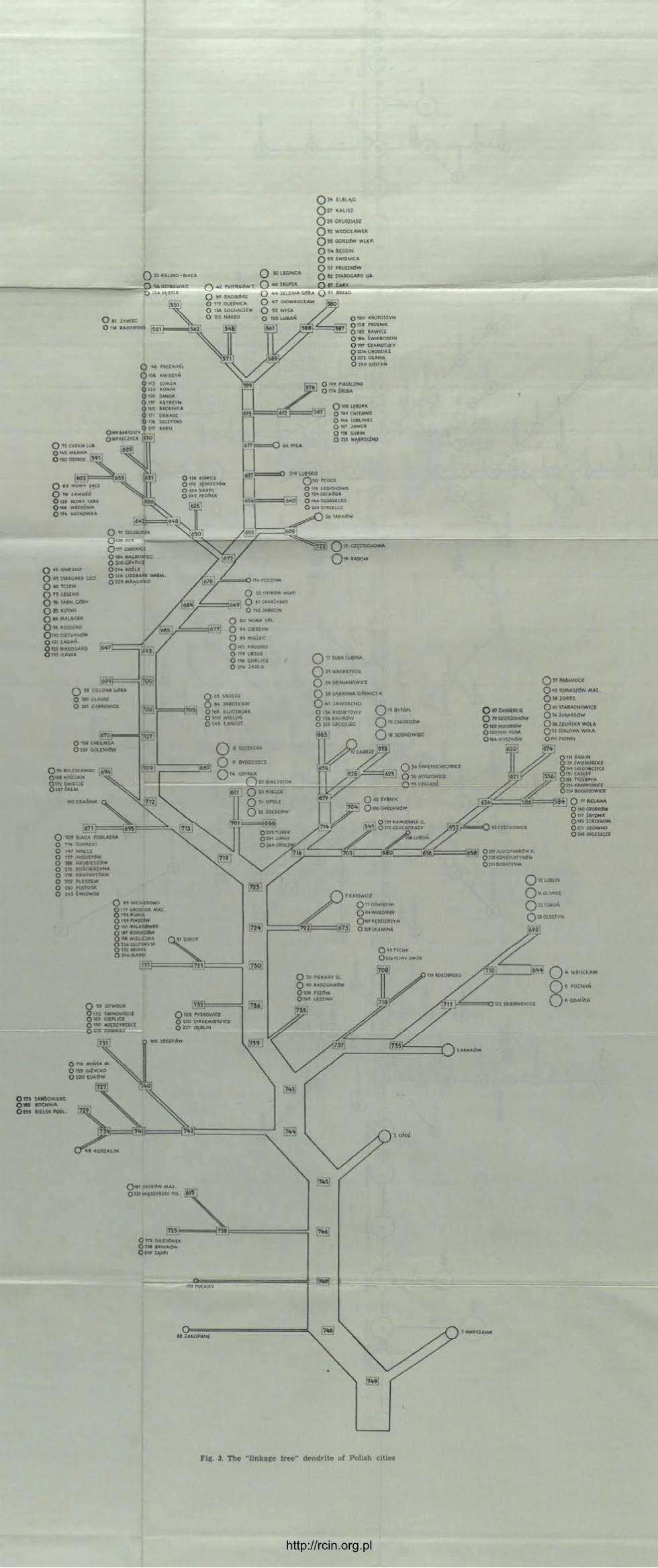
http://rcin.org.pl

194 S T A N I S L A W LEWIŃSKI
struction is as follows. By the "classical" method, the smallest value (but not "0") of each column is selected. The respective numbers of the column and of the row which crosses it are the number of two towns, which are drawn on a diagram and connected with a line, the length of it being proportional to the distance between the points. The connecting of the points is to continued until all towns have been connected into one set. It must be remembered, though, that in the course of constructing the dendrite the line which connects the points must never close up into a circuit. At this place, two explanations must be added:
— In the linkage tree method, the two selected points are connected with one another and their mean values are calculated; whereas in the Wroclaw method one does not calculate the mean values, but treats all points as corners of the graph;
— In using the computing machine, the "classical" method was not applied; all distances f rom matrix C were rearranged according to the increasing order of their values and selected in succession, each time checking whether the new connection does not close the circuit.
The dendrite obtained is presented in Fig. 3. The towns have been presented as circles containing the statistical
number of the town ind its name. The size of the circle is proportional to the number of inhabitants of
the town. The length of the segment connecting two towns and the number written at it denote the taxonomic distance between these towns.
D I V I S I O N O F T H E D E N D R I T E I N T O P A R T S
According to the preliminary assumptions, the Wroclaw dendrite was to be divided into parts by cutting the longest segments. However, this manner of dividing can be applied only when the set under exa-mination consists of several entirely different types, and difficulties arise in case of objects which have features common to more than one type. Our situation, though, is different. There is a very large group of ave-rage, middle-sized towns, which have almost all functions studied, but on an average level. This group of towns constitutes the centre of the set. By cutting of the longest connections a few of the most specialized towns will be separated from the set, but the set will not be divided into parts by this. Therefore, another method has been used in the division of the Wroclaw dendrite. In the set of towns studied we have separated a group of towns which have been less then 1.00 from the theoretically average town (the "ideal" average town is in the centre of the system of co-ordinates and all its features are determined by the normalized
http://rcin.org.pl

T A X O N O M I C M E T H O D S 195
value 0.00000). The division of the dendrite was started by separating a group of average towns on it. The separation of these towns has resulted in partitioning the whole dendrite into subsets. Next, we analyzed all features of each subset and established which feature or features were decisive in the separation of them.
In our set, the following have been distinctly separated: industrial towns (together with a subgroup of mining towns), big cities with well developed functions of science and of construction, and a few groups of small towns such as agricultural and services towns, and dormitory towns.
DIFFERENCES BETWEEN THE WROCLAW TAXONOMY AND THE LINKAGE TREE
In conclusion, we wish to present briefly the differences between the Wroclaw taxonomy and the linkage tree method.
Both methods have the same purpose, namely: (1) to group the objects of a population by an analysis of the positions of their individual points; (2) to separate typical groupings; (3) to divide the population into parts and to order them.
However, the realization of this purpose differs somewhat in both methods. It seems that the most important differences between the two methods can be reduced to the manner of establishing the features, and the manner of the graphic presentation of results.
In the Wroclaw taxonomy, factor analysis is not undertaken, but distances between points are calculated and all features under exami-nation are taken into account after standardization for achieving com-parability.
It seems that from the mathematical point of view both methods are correct. Standardization enhances the significance of those features which are more differentiated, but this is in accordance with the previous assumption that the set should be divided on the basis of those features that are different.
An advantage of the solution offered by the Wroclaw taxonomy is its inexpensiveness and ease of calculation. Standardization of features can be accomplished easily even on the smallest computer, and, in studying small sets even an ordinary office desk calculator will do. Factor analysis is much more complex and requires large computers and programs.
The other essential difference consists in the respective presentation of the sets.
The linkage tree method renders a hierarchy of points and makes possible a univocal division of the set in accordance with Aristotle's
13 http://rcin.org.pl
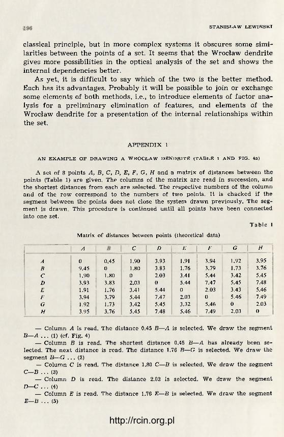
80 S T A N I S L A W LEWIŃSKI
classical principle, but in more complex systems it obscures some simi-larities between the points of a set. It seems that the Wroclaw dendrite gives more possibilities in the optical analysis of the set and shows the internal dependencies better.
As yet, it is difficult to say which of the two is the better method. Each has its advantages. Probably it will be possible to join or exchange some elements of both methods, i.e., to introduce elements of factor ana-lysis for a preliminary elimination of features, and elements of the Wroclaw dendrite for a presentation of the internal relationships within the set.
APPENDIX 1
A N E X A M P L E O F D R A W I N G A W R O C L A W D E N D R I T E ( T A B L E 1 A N D F I G . 4a)
A set of 8 points A, B, C, D, E, F, G, H and a matrix of distances between the points (Table 1) are given. The columns of the matrix are read in succession, and the shortest distances from each are selected. The respective numbers of the column and of the row correspond to the numbers of two points. It is chacked if the segment between the points does not close the system drawn previously. The seg-ment is drawn. This procedure is continued until all points have been connected into one set.
Table 1
Matrix of distances between points (theoretical data)
A C D E F G H
A 0 0,45 1.90 3.93 1.91 3.94 1.92 3.95 B 9.45 0 1.80 3.83 1.76 3.79 1.73 3.76 C 1.90 1.80 0 2.03 3.41 5.44 3.42 5.45 D 3.93 3.83 2.03 0 5.44 7.47 5.45 7.48 E 1.91 1.76 3.41 5.44 0 2.03 3.43 5.46 F 3.94 3.79 5.44 IM 2.03 0 5.46 7.49 G 1.92 1.73 3.42 5.45 3.32 5.46 0 2.03 H 3.95 3.76 5.45 7.48 5.46 7.49 2.03 0
— Column A is read. The distance 0.45 B—A is selected. We draw the segment B—A . . . (1) (cf. Fig. 4)
— Column B is read. The shortest distance 0.45 B—A has already been se-lected. The next distance is read. The distance 1.76 B—G is selected. We draw the segment B— G . . . (2)
— Column C is read. The distance 1.80 C—B is selected. We draw the segment C—B . . . (3)
— Column D is read. The distance 2.03 is selected. We draw the segment D—C . . . (4)
— Column E is read. The distance 1.76 E—B is selected. We draw the segment E—B ... (5)
http://rcin.org.pl

T A X O N O M I C M E T H O D S 197
— Column F is read. The distance 2.03 E—F is selected. We draw the segment E—F ... (6)
— Column G is read. The distance 1.73 G—B has already been selected. The distance 1.92 closes the circuit A—B—G. We select the distance 2.03 G—H. The segment G—H is drawn . . . (7). The set has been connected into one whole. Stop.
Notice: In case a computing machine is used, it is more convenient not to read the columns successively but to sort anew all distances written in one half of the matrix and, after arranging them in an increasing order, to read them suc-cessively.
A S I M P L I F I E D E X A M P L E I L L U S T R A T I N G T H E D I F F E R E N C E B E T W E E N T H E W R O C L A W D E N D R I T E A N D T H E L I N K A G E T R E E
The difference between both types of pictures can be illustrated by a fairly simplified example.
We are given a set of 8 points (e.g., areas) A, B, C, D, E, F, G, H. Each area is characterized by 3 features which correspond to certain functions, e.g., those of industry, services, and agriculture. The data are presented in Table 2. The indexes of the first two areas A and B are on much the same level. The remaining 6 areas
Fig. 4. A simplified example illustrating the difference between the "Wroclaw den-drite" (a) and the "linkage tree" (b).
can be divided into 3 groups with the function of industry predominant in C, D, that of services predominant in E, F, and that of agriculture predominant on G, H. Within each of these groups, two levels of intensity — the average (C, E, G) and the high (D, F, H) — occur.
If w e carry out the calculations and draw the dendrites by the two taxonomic methods described, we shall obtain two different pictures (Figs. 4a, 4b).
APPENDIX 2
http://rcin.org.pl

198 S T A N I S L A W L E W I Ń S K I
In che Wrocław dendrite, the "average"', non-specialized areas are located in the centre. Three different functions diverge radially from the centre. The farther from the centre, the more specialized areas occur.
In the picture drawn by the linkage tree method, the average areas are loca-ted on the very top of the tree. The remaining areas are divided into several storeys. The less specialized areas are located on the higher storeys, whereas the more specialized areas are placed on the lower ones.
Table 2
Values of standardized features (theoretical example)
Points Features (areas) Industry Services Agriculture
A - 0 . 7 . . - 0 . 7 . . - 0 . 7 . . B - 0 . 5 . . - 0 . 5 . . - 0 . 5 . . C 1.0 . . - 0 . 7 . . - 0 . 7 . . D 3.0. . - 0 . 7 . . - 0 . 7 . . E - 0 . 7 . . 1.0. . - 0 . 7 . . F - 0 . 7 . . 3.0. . - 0 . 7 . . G - 0 . 7 . . - 0 . 7 . . 1.0. . H - 0 . 7 . . - 0 . 7 . . 3.0 . .
If the linkage tree suggests a side-view of a tree, the Wroclaw dendrite may sometimes resemble a bird's-eye view of it.
Our example is obviously very simplified; it is intended to present the prin-ciple of division itself. Actually, the situation is more complex. We hawe to take into account more features and these may overlap with one another. In effect, both pictures are much more complex, though the principle of construction does not change considerably.
http://rcin.org.pl

G E O G R A P H I A P O L O N I C A 15
U R B A N G R O W T H A N D T H E C O N C E P T O F F U N C T I O N A L R E G I O N *
D . M I C H A E L R A Y
Urban growth is dependent upon the number and types of goods and services provided for functional regions and is related to the size and population of the functional regions served. The usual cliche is that cities do not thrive where people merely take in one another's washing. "Cities do not grow up of themselves. Countrysides set them up to do tasks that must be performed in central place" 1. The tasks set reflect geogra-phic location. There is, therefore, a sequential relationship between geographic location, urban functions, functional regions and urban growth. The form of the sequential relationship is traced in this biblio-graphic essay by examining the nature and type of urban functions and functional regions, and by reviewing the contribution of location theories to understanding the size and spacing of urban functions and urban places. The relationship is then illustrated by focusing attention on one area, Eastern Ontario, where urban growth has been retarded by the slow expansion of manufacturing industry and is dependent largely upon the central-place functions performed.
* The research on industrial location in Ontario was supported by the (Ame-rican) Social Science Research Council. The research on consumer travel behavior was conducted at the University of Ottawa with the assistance of students of the Department of Geography, including Gary Nadon, Brendon M. Hamill and Carl Smith. Additional maps and diagrams were prepared at Spartan Air Services by Robert Carstens with support from Agricultural and Rural Development Admini-stration. I also gratefully acknowledge the valuable comments and criticisms re-ceived from Brian J. L. Berry, Chauncy D. Harris, Harold M. Mayer, Gerard Rush-ton, Lerov Stone and Maurice Yeates.
1 Mark Jefferson, The Distribution of the World's City Folks: A Study in Comparative Civilization, Geographical Review, XXI, 1931, p. 453.
http://rcin.org.pl

200 D. M I C H A E L R A Y
URBAN FUNCTIONS
The relationship between urban growth ad functional regions is clarified by partitioning urban functions into those that are city-serving, or non-basic activities, and those that are city-forming or basic 2. Non--basic activities are those services and functions that a city provides for its resident population and are not shaped by the location of the city. "Basic urban functions involve the processing or trading of goods or the furnishing of goods and services for residents or establishments lo-cated outside of the urban area" 3.
Basic activities show greater contrasts among urban places than do non-basic activities and thereby serve as a valuable guide to functional classification4. Examination of basic functions indicates four distinct types of city, (1) central places — providing retail and other tertiary services to their trade areas, (2) transportation centres, (3) manufacturing centres and (4) special-function centres, such as government, administra-tive, religious or military centres 5.
The distribution of basic functions among cities is related to the spa-tial elasticity of demand for those functions. The spatial elasticity of demand is the measure of "distance decay", or the rate at which supply of a good or service f rom a city declines with distance from that city. Where the elasticity and hence the distance decay are high, as in the case of low-order retail services, the function has a ubiquitous distri-bution. For high-order manufactured goods, the distance decay is low, and the function becomes sporadic and found in only a few urban places.
Urban places with economic functions of a ubiquitous nature can be expected to serve only small functional regions, to have a limited growth potential and to have a regular distribution pattern. Accelerated urban growth depends upon the ability of a city to develop "national-market
2 The economic base concept is reviewed by Harold M. Mayer, A Survey of Urban Geography, The Study of Urbanization, edited by Philip M. Hauser and Leo F. Schnore, John Wiley and Sons, New York, 1965, pp. 83—86; Wilber R. Thompson, A Preface to Urban Economics, John Hopkins Press, Baltimore, 1965, pp. 27—30; and O. D. Duncan et al., Metropolis and Region, John Hopkins Press, Baltimore, 1960, pp. 23—36. Five studies on the economic base of cities are reprinted in Harold M. Mayer and Clyde F. Kohn (eds.), Readings in Urban Geography, The University of Chicago Press, Chicago, 1959, pp. 85—126.
3 Mayer, op. cit., p. 83. 4 For a review of urban classification systems, see Robert H. T. Smith, Methods
and Purpose in Functional Town Classification, Annals of the Association of Ame-rican Geographers, Vol. 55, September 1965, pp. 539—548.
5 Chauncy D. Harris and Edward L. Ullman, The Nature of Cities, Annals of the American Academy of Political and Social Science, Vol. 242, November 1945, pp. 7—17; reprinted in Mayer and Kohn, op. cit., pp. 277—280.
http://rcin.org.pl

JJRBAN G R O W T H A N D T H E C O N C E P T O F F U N C T I O N A L R E G I O N 201
activities" which have a low distance decay. Isard relates the population rank of a city within a country to the number of national-market area activities which it captures, while at the same time retaining all "non--national" activities 6.
The concept of basic functions thus stresses the economic ties which bind a city to its region, and which link urban growth to the size of the region. Unfortunately, urban economic base studies have not generally concerned themselves with identification of the areas to which basic fonctions export, nor with the concept of functional region 7. The section which follows reviews the concept of region and the factors influencing the location of boundaries of functional regions.
THE CONCEPT OF FUNCTIONAL REGION
The area over which an urban centre provides services and functions is termed a functional or nodal region, or simply market area or hinter-land. More generally, a functional region is "an area in which one or more selected phenomena of movement connect the localities within it into a functionally organized whole" 8. Except for the smallest urban centres and for the lowest order functions, the market area includes other urban places as well as rural areas.
The "outer (or farthest possible) range" of a functional region is defined as the point at which transportation costs, to the consumer or producer, reduce effective demand or supply to zero. The distance of the autor range from the urban centre depends on the spatial elasticity of demand, or distance or interactance decay, of the function. The lower the distance decay, the greater the agglomeration or concentration of the industry and the larger the economic region.
The higher the distance decay, the less likely it is that the economic
6 Walter Isard, Location and Space Economy, Massachusetts Institute of Tech-nology Press, Cambridge, Massachusetts, 1956, pp. 55—60.
7 Duncan, et. al., op. cit., p. 33. 8 Brian J. L. Berry and Thomas D. Hankins, A Bibliographic Guide to the Eco-
nomic Regions of the United States, Department of Geography, Research Series No. 87, University of Chicago, Chicago 1963, p. x. See also Derwent Whittlesey, The Regional Concept and the Regional Method, in American Geography: Inventory and Prospect edited by P. E. James and C. F. Jones, Syracuse University Press, Syra-cuse, 1954, pp. 21—68; and Richard S. Thoman and Gerald McGrath, Re-gional Statistics and Their LTses: A Geographic Viewpoint, Regional Statistical Stu-dies, edited by S. Ostry and T. Rymes, University of Toronto Press, Toronto, (forth-coming).
http://rcin.org.pl
202 D. M I C H A E L . R A Y
region will extend to the "outer range"-. As functions disperse, to pro-duce a true network of regions rather than concentrating in a punctiform agglomeration, the more likely it is that the "real range" will be set by competition from other urban centres offering the same function. The "real range" occurs at the line where total costs for a service or good from two competing centres, that is, the cost of the good at each centre plus transportation cots are equal. The line along which alternate centres can provide a function at equal cost is termed the "line of indifference".
A review of location theories, in the next section, suggests that the "line of indifference" delimiting a functional region is rarely sharp Complicating factors, such as multi-purpose travel behaviour, tend to produce a decreasing allegiance away f rom the region's urban centre until a zone of indifference is reached.
Furthermore, both the outer range and the real range of a function may be changed by pricing policy. An equalizing delivered-price system, or single or multiple basing-point systems of pricing practically elimina-tes market boundaries and may extend the range to the national market area 9. Basing-point price systems have been used extensively by pro-cessing industries to retain their locational adventage and to maintain their market area in face of possible competition from f i rms at new loca-tions 10. Basing-point price systems have now been declared illegal by the United States Supreme Court, and the market areas there can be ex-pected to become more sharply defined n .
An examination of the relationship between functional and other types of regions shows that the size and shape of market areas and func-tional regions is not determined by economic factors alone. Functional regions are conceptually distinct f rom the two other types of regions recognized by geographers but they are not independent of them.
The other two uses of the term "region" that geographers distinguish are the general region, and the homogeneous or formal region. The first is most frequently used in Canada to refer to an administrative unit or contiguous group of units, such as a province or a group of counties or municipalités. A homogeneous region is "an area within which the varia-tions and co-variations of one or more selected characteristics fall within
9 See Melvin L. Greenhut, Plant Location in Theory and Practice, The Uni-versity of North Carolina Press, Chapel Hill, 1956, pp. 23—83, and Appendix V, pp. 308—316.
10 Gardner Ackley, Price Policies, Industrial Location and, National Resources, National Resources Planning Board, Washington, 1942, pp. 302—303.
11 Frank A. Fetter, Exit Basing Point Pricing, American Economic Review, Vol. 38, 1948, pp. 815—827.
http://rcin.org.pl

J J R B A N G R O W T H A N D T H E C O N C E P T OF F U N C T I O N A L R E G I O N 203
some specified range of variability around a norm, in contrast with other areas that fall outside the range" 12.
Functional regions are affected by the homogeneous and administra-tive regions in which they are located. Berry, for example, has establis-hed that different systems of cities, and different sizes od functional regions can be identified for different homogeneous agricultural regions by the different farm population densities supported in each agricul-tural region 13. This study shows that Eastern Ontario may be divided into two homogeneous cultural regions and that the boundary of some functional regions is displaced from the line of economic indifference to the cultural boundary.
The boundaries of homogeneous physical regions, instead of delimi-ting the functional boundaries of existing towns, may lead to the esta-blishment of new urban places to perform transportation functions at break of bulk points, such as coastlines, or trade between the contrasted products of different physical regions 14.
The boundaries of political regions tend to restrict functional regions. Losch illustrates this effect by mapping the financial sphere of influence, or functional region of El Paso, on the United States-Mexican border 13. The reduced market area south of the border accords with his theoretical statements 16. Mackay succeeded in measuring the reduction interaction across the Quebec-Ontario and the Quebec-United States borders 17.
Although the size and shape of functional regions is modified by non--economic factors, economic location theories do contribute to an under-standing of the distribution of functions among urban places and hence of the interrelationship between urban growth and functional region. Location theories should relate urban functions to location; unfortuna-tely, research has tended to treat function and location as separate problems.
12 Berry and Hankins, op. cit., p. x. 13 Brian J. L. Berry, Cities as Systems Within Systems of Cities, Papers and
Proceedings of the Regional Science Association, Vol. 13, 1964, pp. 147—163. 14 Gordon East, The Geography Behind History, Nelson and Sons, London 1938,
pp. 91—92. 15 A. Lösch, Die räumliche Ordnung der Wirtschaft. Transl. W. Woglom and
W. Stolper, The Economics of Location, Yale University Press, New Haven, 1954, p. 448.
16 Ibid., p. 341. 17 J. Ross Mackay, The Interactance Hypothesis and Boundaries in Canada:
A Preliminary Study, Canadian Geographer, No. 11, 1958, pp. 1—8. Julian V. Minghi reviews studies of political boundaries as locational factors in, Boundary Studies in Political Geography, Annals of the Association of Amercian Geographers, Vol. 53, 1963, pp. 407—428.
http://rcin.org.pl

204 D. MICHAEL. R A Y
LOCATION THEORIES
The location theories reviewed in this section, central place theory and industrial location theory, apply to only two of the four main urban types noted earlier, namely, central places and manufacturing centres. These two types are the most important, however. Lampard, for example, divides the history of definitive urbanization into two phases, classic and industrial, with central places dominating in the first phase, and the se-cond phase witnessing the rise of the industrial city 18. The theoretical review attempts to explain differences in the size and spacing of central places and manufacturing centres. It emphasizes one common element in the two bodies of theory, namely, distance decay or the spatial elasticity of demand.
C E N T R A L P L A C E T H E O R Y
The foundations of central place theory were laid by Walter Chris-taller in 1933 19. Berry and Pred have summarized the six main features of Christaller's theory as follows: (1) The main function of a city is to be a central place providing goods and services for the market area, and that cities are located central to the maximum profit area they can com-mand. (2) The greater a city's centrality, the higher its order. (3) Higher order places offer a larger range of goods and services, but are more widely spaced than lower order places. (4) Low order places offer goods purchased frequently or convenience goods. (5) A hierarchy of central places exists. (6) Three hierarchies may be organized according to, (a) a market principle, (b) a transportation principle, and (c) an admini-strative principle 20.
Losch elaborated Christaller's work by demonstrating that Christal-ler's hexagonal market areas were optimal for consumers and entrepre-neurs 21. He also showed that Christaller's three hierarchies of market areas were special cases of the ten smallest hexagonal market areas that
18 Eric Lampard, Historical Aspects of Urbanization, The Study of Urbanization, op. cit., pp. 519—554.
19 Walter Christaller, Die zentralen Orte in Süddeutschland, Gustav Fischer Verlag, Jena, 1933. Christaller's concepts were introduced to the English language literature by Edward Ullman, A Theory of Location for Cities, American Journal of Sociology, Vol. 46, May 1941. pp. 835—864, reprinted in Mayer and Kohn, op. cit., pp. 202—217.
20 Brian J. L. Berry and Allen Pred, Central Place Studies: A Bibliography of Theory and Applications, Regional Research Institute, (Philadelphia, 1965), pp. 3—4.
21 A. Lösch, op. cit., pp. 105—114.
http://rcin.org.pl
J J R B A N G R O W T H A N D T H E C O N C E P T OF F U N C T I O N A L R E G I O N 205
combine to form an economic landscape with six city-rich and six city--poor sectors around the regional capital 22.
Berry and Garrison have shown that Christaller's theory is more limited than Christaller thought, because not all cities are primarily central places; it is also more general than Christaller believed because it applied to shopping centres within cities 23. This broader application of central place theory emerges when it is reformulated in terms of its two essential concepts, "range of a good" and "threshold". The outer range of a good is the maximum distance that persons travel for that good. The inner range of the good is the distance enclosing the minimum num-ber of consumers required to support the function. Threshold is "the minimum amount of pruchasing power necessary to support the supply of a central good f rom a central place" 24. The numbre of establishments pro-viding a function that can be supported in an area is equal to the total purchasing power divided by the threshold. For higher order functions, requiring large thresholds, fewer establishments can be supported. A hie-rarchy of central places and of shopping centres within central places emerges which is inducated by the number of central functions that a central place or shopping centre contains, and by the total market area and total population which it serves.
Figure 1 illustrates the relationship of trade area served to total po-pulation served for systems of central places in six homogeneous re-gions 25. The structure of these systems shows a remarkable consistency. The hierarchy of the central places in all regions, except Eastern Ontario, lias been identified by use of a direct factor analysis. The upper limits of the groups of villages, towns, cities and regional capitals are linked by straight lines which intersect the Eastern Ontario system at the points suggested for it by changes in central functions performed.
Examine the central place system for the agricultural regions on Fig. 1. The higher the gross population density, the smaller the functional region but the larger the population served by a centre at a given level of the urban hierarchy. Thus, the spacing of these central places increases
22 Ibid., pp. 114—137. 23 Brian J. L. Berry and William L. Garrison, A Note on Central Place Theory
and the Range of a Good, Economic Geography, Vol. 34, October 1958, pp. 304—311; Brian J. L. Berry and William L. Garrison, Recent Developments of Central Place Theory, Papers and Proceedings of the Regional Science Association, Vol. 4, 1958, pp. 107—120.
24 Ibid., p. 111. 25 Figure 1 is copied from B. J. L. Berry and H. Barnum, Aggregate Relations
and Elemental Components of Central Place Systems, Journal of Regional Science, Vol. 4, Summer 1962. Fig. 2 p. 40 with the Eastern Ontario central places added.
http://rcin.org.pl
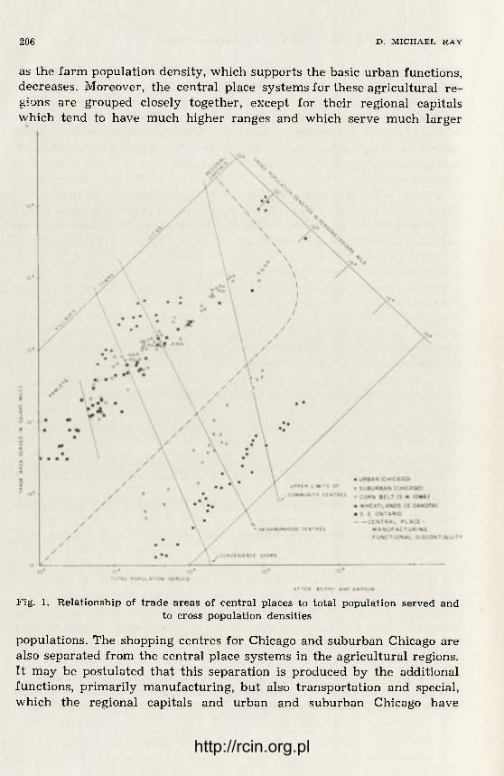
206 D. M I C H A E L . R A Y
as the farm population density, which supports the basic urban functions, decreases. Moreover, the central place systems for these agricultural re-gions are grouped closely together, except for their regional capitals which tend to have much higher ranges and which serve much larger
Fig. 1. Relationship of trade areas of central places to total population served and to cross population densities
populations. The shopping centres for Chicago and suburban Chicago are also separated from the central place systems in the agricultural regions. It may be postulated that this separation is produced by the additional functions, primarily manufacturing, but also transportation and special, which the regional capitals and urban and suburban Chicago have
http://rcin.org.pl
J J R B A N G R O W T H A N D T H E C O N C E P T OF F U N C T I O N A L R E G I O N 207
acquired. The separation may be termed, therefore, a "functional dis-continuity"; urban places may cross it and extend their area or population served only by obtaining these additional functions.
The lowest total population served by a level of the hierarchy in Fig. 1 may be used as a measure of "threshold" or "condition of entry", pro-vided that it is assumed that each purchasing power is homogeneously distributed. The maximum range of each level of the hierarchy coincides with the threshold value of the next higher level of the hierarchy. The range of any level of the hierarchy cannot exceed the threshold of a higher level of any length of time before the additional functions that can be supported by the larger population are acquired, and the central place advances to the next higher order of the hierarchy. The growth of the central places is limited by the size of the population in the maxi-mum profit area that each place can command. An equilibrium neces-sarily exists between the size and the spacing of the central places.
The equilibrium in a central place system between the size and the spacing of the central places is attained when the demand density per unit area lifts the range of the good above the threshold. Where the range of a good includes less purchasing power than the threshold value, activities are mobile. Stine has illustrated this case in a study of travell-ing merchants and periodic markets in Korea2 6 . The distance between the market centres that a mobile merchant must serve is dependent on the range of the good. The number of market centres he must serve is dependent on the threshold. Activities survive only where the cycle of the merchant 's movements is short enough to offer to the customer the requisite frequency for that service and where the marginal costs of serving the additional markets to reach the threshold value do not exceed the resulting marginal revenue. Mobile markets are replaced by perma-nent markets and a regular pattern of central places crystallizes when the increase in demand density per unit area lifts the range of the good above its threshold.
Changes in retailing technology, in population density and in income af ter the equilibrium between range and threshold is established and permanent markets or central places created produce shifts in the equi-librium 27. Few studies of changes in central place systems have been made and all have encountered serious diffuculties because of data defi-
26 James H. Stine, Temporal Aspects of Tertiary Production Elements in Korea, in Forrest R. Pitts (ed.), Urban Systmes and Economic Development, School of Bu-sines Administration, University of Oregon, Eugene, Oregon, 1962, pp. 68—88.
27 Brian J. L. Berry, Commercial Structure and Commercial Blight, Department of Geography Research Series, No. 85, University of Chicago, Chicago 1963, pp. 161—177.
http://rcin.org.pl

208 J J R B A N G R O W T H A N D T H E C O N C E P T OF F U N C T I O N A L R E G I O N 208
ciencies and because of changes over time in types of function and insti-tutions providing central functions 28. Nevertheless, these studies suggest that villages will share the same fate as hamlets, now in the final throes of decline, as a result of advances in technology and the consequent im-provements in transportation and increased specialization in retailing.
The provision of central functions in larger but fewer stores is paral-leled in metropolitan areas. Berry find that a 5.87 per cent decrease per year in the number of retail establishments in Chicago can be attributed to technological t rends2 9 . These technological effects are modified by changes in population density and income. Changes of one per cent in real income have produced an average 0.87 per cent change in number of establishments. The net effect of technology and income changes in Chicago has been to produce a 2 per cent decline in retail establishments in higher income communities, a 4 per cent decline in low income com-munities, and a 5 per cent decline in transition communities with falling socio-economic status.
By undermining villages and hamlets, as well as convenience shops in larger urban centres, changes in retailing technology are producing an effect on the growth of central places similar to Wilbur Thompson's "urban ratchet" in growth of metropolitan centres 30. Central places that have failed to reach "town" or higher status can expect fu ture functional development only if technological effects are off-set by a growing po-pulation and increasing socio-economic status in the functional region that they serve.
The focus by Berry and Garrison on the key concepts in central place theory of range of the good and threshold has been used to stress the relationship between growth of central places and number of central functions, and to reveal the equilibriums within systems of central places between central functions and population of functional regions. Further insights on the relationship between city and region are obtained by re-
28 Jaob Spelt, Urban Development in South Central Ontario, Van Gorcum and Company, Assen, Netherlands, 1955; H. Carter, Urban Grades and Sphere of Influ-ence in Southwest Wales, Scottish Geographical Magazine, Vol. 71, 1955, pp. 43—48; H. Carter, The Urban Hierarchy and Historical Geography, Geographical Studies, Vol. 3, 1956, pp. 85—101; R. E. Dickinson, The Distribution and Functions of the Smaller Urban Settlements in East Anglia, Geography, Vol. 17, 1932, pp. 19—31; R. E. Dickenson, Markets and Market Areas of East Anglia, Economic Geography, Vol. 10, 1934, pp. 172—182; Brian J. L. Berry, The Impact of Expanding Metropoli-tan Communties Upon the Central Place Hierarchy, Annals of the Association of American Geographers, Vol. 50, 1960, pp. 112—116.
29 Berry, Commercial Structure and Commercial Blight, p. 173. 30 Thompson, op. cit.
http://rcin.org.pl
J J R B A N G R O W T H A N D THE CONCEPT OF F U N C T I O N A L REGION 209
viewing range of the good in the framework of the broader concept of distance decay within which range of the good may be embodied.
Distance or interactance decay measures the decline in the demand for goods and services at a central place with increasing distance f rom it. Distance decay is equivalent, therefore, to the spatial elasticity of de-mand. Distance or interactance decay is the structural element of the interactance or gravity concept which states that interaction between two masses is proportional to their sizes and inversely proportional to some function of their distance apart3 1 . The interactance concept was first applied in central place studies by Reilly in 1929 to delimit the line of indifference, or the functional boundary between competing central places 32.
Clearly, the aggregate movement of consumers into a central place for all goods and services decreases with increasing distance f rom it. A central place offers all services with thresholds below the total pur-chasing power of the population located within its maximum functional region. But not all services are provided to all customers within that maximum functional region f rom a single central place. Other, smaller central places nest within its maximum functional region to provide lo-wer-order services. The empirical study of Eastern Ontario in this paper shows, for example, that city-level central places do not provide food, auto repair, banking and other lower-order services to all of their medical and dental services regions. The frequency and intensity of aggregate consumer travel to cities drops beyond the ranges where they can provide hamlet, village, and town level functions.
Distance decay has also been observed in the pattern of consumer travel behaviour for single services. Nystuen found in an analysis of consumer travel in Cedar Rapids, Iowa, that distance decay was higher for single purpose trips than for multipurpose 33. The average distances travelled for multi-purpose shopping trips was greater because househol-ders may bypass the nearest store offering one service they need and instead "attempt to get maximum return from total travel effort needed to fulfill all the purposes combined on the trip" 34.
More recently, Rushton has determined the effect of differences in
31 See Walter Isard et al., Methods of Regional Analysis: An Introduction to Regional Science, Massachusetts Institute of Technology Press, Cambridge, I960, pp. 494—499.
32 W. J. Reilly, Methods for the Study of Retail Relationships, University of Texas Bulletin, Vol. 2944, 1929.
33 William L. Garrison et. al., Studies of Highway Development and Geographic Change, University of Washington Press, Seattle, 1959, p. 213.
34 Ibid., p. 212.
14 G e o g r a p h i a P o l o n i c a t . 15
http://rcin.org.pl

2 1 0 D. MICHAEL. R A Y
family income and in grocery expenditures on travel for grocery pur -chases in Iowa State and has developed a space preference model which reveals a decreasing allegiance to a central place with increasing distance from it3 5 . Applying this model to the town of Humboldt, Iowa, he pre-dicts that beyond five miles of Humboldt, more than 25 per cent of fa-milies have a secondary grocery expenditure town and near the boun-daries of its functional region for grocery services, more than 75 per cent of the families have a secondary expenditure town 36.
In summary, growth of central places is related to the equilibrium between the population served and the functions acquired. The greater the population that can be served f rom a central place in competition with other places, the higher the order of the functions that can be sup-ported. Higher order functions have higher thresholds and are more widely spaced. The equilibrium between the population served and funct-ions acquired is translated into an equilibrium in the size and spacing of cities. Both equilibria are shifting ones, primarily because of changing technology. An urban ratchet effect may be observed in which central places with only hamlet or village status are usually slipping back, while higher-order centres have their growth achievements locked in. A func-tional discontinuity is evident between the ranges and population served by regional capitals and metropolitan and suburban shopping centres, and by other central places in agricultural regions. This suggests that a marked growth of an urban place and its functional region occurs when central place functions are supplemented by manufacturing and other activities. The acquisition of manufacturing activity and the acceleration of urban growth may be explained by the industrial location theories reviewed in the next section.
I N D U S T R I A L L O C A T I O N T H E O R I E S
The contribution of industrial location theories to understanding ur-ban growth is limited by their restricting assumptions and by their con-cern with the location of individual establishments. These theories cannot be extended easily to explain regional patterns of manufacturing location in the real-earth space.
Alfred Weber, in his seminal work, is concerned primarily with deter-
35 G. Rushton, Spatial Pattern of Grocery Purchases by the Iowa Rural Popu-lation, Studies in Business nd Economics, New Series No. 9, The University of Iowa, Iowa City, 1966.
36 Ibid., p. 59.
http://rcin.org.pl
U R B A N G R O W T H A N D T H E C O N C E P T OF F U N C T I O N A L R E G I O N 211
mining the location of lowest production costs for an establishment ser-ving a single city market with inelastic demands 37. An industrial plant would deviate from the point of lowest aggregate transportation costs and of labour costs to serve two or more city markets only where the deviation costs are exceeded by the agglomeration economies, or econo-mies of scale. Weber treats agglomeration economies as a local factor operating within the general framework formed by the regional factors, transportation and labour costs 3S.
Later studies extended the market f rom a single point to a straight line and dealt with the interdependence of two establishments under nonelastic and elastic market conditions 39. Fetter was the first to de-termine the size and shape of market areas for given plant locations on a homogeneous plain 40.
Lösch has criticized the unrealistic assumption and the unusual lo-cational problems in these studies and goes on to develop a three-level typology of industrial concentration and size of economic region. The highest level is termed a "punctiform agglomeration" and occurs where the individual locations of the function coincide in a single urban centre or group of centres to serve the national market. Lösch gives the example of "factories producing men's collars, practically all of which are situ-ated in Troy, New York, but whose market includes the whole of the United States." 41 An intermediate level of concentration identified as "areal agglomeration", is subdivided into belt locations and district lo-cations. In belt locations, the market network is compressed, such as cotton gins in the cotton belt. In districts the centres are compressed, but the markets are separated. An example is coal mines in a coal-field. The lowest level of concentration is for commodities such as bread. Lösch describes bakeries as having no concentration and "forming a true network of regions".42
Lösch's typology may be interpreted as selecting three critical stages
37 Alfred Weber, The Theory of Location of Industries, 1909, translated by Carl J. Friedrich, University of Chicago Press, Chicago, 1929. Reviews of this and other studies are contained in William L. Garrison, Spatial Structure of the Economy, Annals of the Association of American Geographers, Vol. 44, 1959, pp. 232—239, 471—482; Vol. 50, 1960, pp. 357—373.
38 Ibid., p. 124. 39 H. Hotelling, Stability in Competition, The Economic Journal, Vol. 39, 1929,
pp. 41—57; A. Smitties, Optimal Location in Spatial Competition, Journal of Poli-tical Economy, Vol. 49, June 1941, pp. 423—440.
40 F. Fetter, The Economic Law of Market Areas, Ouarterly Journal of Econo-mics, Vol. 38, 1924, pp. 520—529.
41 A. Losch, op. ext., p. 11. 42 Ibid.
14* http://rcin.org.pl

212 D. MICHAEL. R A Y
in distance decay, or range of the good, with the highest distance decay for bakeries, and a low distance decay for men's collars.
Harris applied the concepts of distance decay and gravity or interac-tance to measure aggregate accessibility from any point to the total market 4 3 . The measure, termed "market potential" is defined mathemati-cally at a point (Pi) as the sum (I) of each market (M7) divided by its distance (da) f rom that point; that is, market potential 'at Pi=Z{Mj/da)
j where the distance for measuring self-potential (da) is an assigned con-stant. The point of highest market potential for the United States is New York and for Canada, Toronto (see Fig. 2. The distance-decay exponent of 1.42 used in this Figure has been determined f rom analysis of Cana-dian commodity flows). These two points offer the greatest accessibility to the national markets and national market area activities can be ex-pected to gravitate towards them accelerating their rate of growth.
There is evidence that market is growing in importance as a factor in industrial location and that the amount of secondary manufacturing industry that an urban centre can acquire depends on its market poten-tial. The growing importance of market is attributed by Harris to in-creased fabrication in finished products, greater afficiency in the use of raw materials, and improved transportation4 4 . Borts finds that diffe-rences in regional growth patterns are to be „explained by a difference in production functions or in the demand for a region's exports", and his findings provide, "strong support for a model of regional growth based on the demand for a region's exports" 45. Fuchs endorses the role of markets in determining changes in the location of industry 46. Duncan finds that secondary manufacturing is highly correlated with population-potential and that deviations of manufacturing f rom market accessibility are attri-butable to the locational pull of mineral deposits 47.
The market potential concept, introduced into industrial location theory by Harris, cannot explain entirely regional patterns of secondary
43 Chauncy D. Harris, The Market as a Factor in the Location of Industry in the United States, Annals of the Association of American Geographers, Vol. 44, December 1954, pp. 315—348.
44 Ibid. 45 George H. Borts, The Equalization of Returns and Regional Economic Growth,
The American Economic Review; Vol. 50, June 1960, pp. 319, 343. 48 Victor F. Fuchs, The Determinants of the Redistribution of Manufacturing in
the United States Since 1929, The Review of Economics and Statistics, Vol. 44, 1962, pp. 167—177.
47 Duncan et. al., op. cit., pp. 126—128, 165—166, 209—226; and Otis D. Duncan, Manufacturing as An Urban Function: The Regional Viewpoint, Sociological Quar-terly, Vol. 1, April 1960, pp. 75—86.
http://rcin.org.pl

http://rcin.org.pl
214 D. M I C H A E L . R A Y
manufacturing location. In particular, it does not take account of source of capital and industrial organization on location. Hare has stressed the crucial importance of finance capital in economic development, and notes that the origin of finance capital is a more powerful determinant of lo-cation than the so-called "geographic" factors 48. Origin of capital is par-ticularly important where location decisions are made by head offices of multi-establishment firms. These location decisions will reflect the lo-cations of the head office and its establishments, for as Losch has said, "we are largely f ree to select our location. This in influenced, though not dictated, by our place of rigin" 49.
The empirical section of this paper uses the concept of "economic shadow" to measure accessibility to finance capital and entrepreneur-ship 50. Like range of the good and market potential, economic shadow employs the distance decay concept. It states that the likelihood of a ma-nufacturer establishing a branch plant in a city is inversely proportional to that city's distance from the manufacturer. For example, the nu-merical difference between the 98 branch plants in Metropolitan Toronto controlled by head offices in Chicago and the 28 controlled from Los Angeles is largely explained by the greater distance of Los Angeles f rom Toronto. The primary element of economic shadow is sectoral affinity which states that branch plants tend to be located in the sector lying between the head office and the primary market centre within a region. Industrial interactance between a part of a region and a city beyond that region is impeded whenever the primary market centre of the region becomes an intervening opportunity. An "economic shadow" is thus cast over the area lying beyond the spatial sector linking a head office to the primary regional market centre. Urban growth may be retarded in areas of high economic shadow, irrespective of their market potential and accessibility to the national market. Urban growth is concentrated in-stead on what Friedmann and Alonso term "development axes" 51.
Despite the many gaps in the literature, it has been possible to trace the sequential relationship between geographic location, urban functions, functional regions and urban growth. Urban growth depends ultimately on geographical location and accessibility. In the early phases of definitive urbanization, economic foundations of urban growth are low order central
48 F. Kenneth Hare, A Policy for Geographic Research in Canada, The Canadian Geographer, Vol. 8, 1964, p. 115.
49 Losch, op. cit., p. 1. 50 D. Michael Ray, Market Potential and Economic Shadow, Department of Geo-
graphy, Research Series, No. 101, University of Chicago, Chicago 1965. 51 John Friedmann and William Alonso (eds.), Regional Development and Plann-
ing, Massachusetts Institute of Technology Press, Cambridge, 1964, p. 3.
http://rcin.org.pl

J J R B A N G R O W T H A N D THE CONCEPT OF F U N C T I O N A L REGION 215
place functions. Geographic location is then to be interpreted merely as the degree of centrality to the surrounding rural area. Urban growth accelerates where special functions, such as transportation, administra-tive, mining, religious and military are acquired. The growth of these functions must also reflect geographic location to the extent that reso-urces and attributes of an area can be developed beyond local demand only if it is favourably located in relation to other centres of population, even though all other requirements for its growth may be fulfilled.
Technological developments, primarily by improving transportation and reducing the friction of distance, a n i by increasing income and demand density, permit the establishment ox higher-order central func-tions and the creation of a hierarchy of networks of market regions. The geographic location and centrality of an urban place must then be me-asured in terms of larger areas including other urban places.
Once technological developments give rise to the industrial city, geo-graphic location must be interpreted in terms of sub-national and na-tional market areas. Higher order manufacturing has a low distance decay and becomes concentrated into areal and punctiform agglome-rations. The ability of an urban centre capture national and sub--national market area activities and to enjoy substained growth can be measured by its market potential. Nevertheless, urban growth is retar-ded in areas of high economic shadow. These relationships are illustrated in the study on Eastern Ontario, which follows.
EASTERN ONTARIO
T H E L O C A T I O N O F U N I T E D S T A T E S B R A N C H P L A N T S I N S O U T H E R N O N T A R I O
Eastern Ontario lies in the Canadian Heartland, which comprises the densely populated St. Lawrence Lowlands and Southern Ontario, and which contains over half the eighty Canadian cities with populations over 10,000. The heartland stands out as a plateau of high market po-tential (see Fig. 2), and all but two of the cities over 10,000 are classified by Maxwell as having manufacturing as their dominant function (see Table 1).
Southern Ontario has led Canada since Confederation in levels of urbanization and manufacturing. Data released by Stone shows that Ontario has generally been a decade ahead of any other region of Canada in achieving given levels of urbanization and in 1961, was the only pro-vince with more than three-quarters of its population classified as urban (see Table 2).
The considerable post-war growth of secondary manufacturing in-
http://rcin.org.pl

2 1 6 D. MICHAEL. R A Y
Table 1 Functional classification of Canadian cities
Region Central Transpor- | Manufactu- Other Total : place tation ring
Periphery 7 5 18 5 35 Heartland 1 - 43 1 45
1 Total 8 5 61 6 1 80
N o t e : Maxwell uses the minimum requirement approach of Ullman and Dacey to measure functional s t ructure and to classify the cities. The study is for all urban areas with populat ion over 10,000
S o u r c e : J. W. Maxwell, The Functional Structure of Canadian Cities: A Classification of Towns, Geographical
Bulletin, V o l . 7 , N o . 2 , 1965, p p . 7 9 - 1 0 4 .
Table 2
Census years in which Canada and the major regions had reached or surpassed selected levels of urbanization
Levels of urbanization O 25% 35% 50% 65% 75%
Canada Maritimes 1891 1902 1931 1961 —
Quebec 1901 1921 1961 _ ( 2 ) —
Ontario 1881 1891 1911 1941 1961 Prairies 1911 1951 1961 — —
British Columbia 1891 1891 1911 1951 -
N o t e : ( ' ) The level of urbanization is measured by the percentage of populat ion classified as urban . In this table, the symbol ,, —" indicates that the area in question had no i attained the pertinent level of urba-
nization as of 1961, according to the source data . S o u r c e : Table released by Leroy Stone, Demographic Analysis and Research, Census Division, Donominion
Bureau of Statistics, f rom the census monograph on urban development in Canada .
dustry in Canada has continued to be concentrated in parts of Southern Ontario, particularly the Toronto Metropolitan Area and Southwestern Ontario. In Comparison, Eastern Ontario's industrial growth has been retarded.
The sharp contrast between the rates of growth for Southwestern Ontario and Toronto Metropolitan Area, and for Eastern Ontario is not confined to manufacturing. Factor analyses of socio-economic charac-teristics reveal the interdependency of rates of economic growth, po-pulation growth, age and sex stucture, cultural characteristics, and housing conditions, and they indicate that the regional contrasts in rate of economic development consitute the fundamental factor in the geo-graphy of Ontario 52.
52 D. M. Ray and B. J. L. Berry, Socio-Economic Regionalization: A Pilot Study in Central Canada, in Ostry and Rymes, op. cit., B. J. L. Berry, Identification of Declining Regions: An Empirical Study of the Dimensions of Rural Poverty, in
http://rcin.org.pl
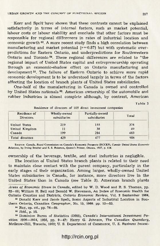
J J R B A N G R O W T H A N D THE CONCEPT OF F U N C T I O N A L REGION 217
Kerr and Spelt have shown that these contrasts cannot be explained satisfactorily in terms of internal factors, such as market potential, labour costs or labour stability and conclude that other factors must be responsible for regional differences in rates of industrial location and economic growth 53. A more recent study finds a high correlation between manufacturing and market potential (r = 0.87) but with systematic over-predictions for Eastern Ontario, and underpredictions for Southwestern Ontario and Toronto54 . These regional differences are related to " the regional impact of United States capital and entrepreneurship operating through an economic-shadow effect on Ontario manufacturing and development5 5 . The failure of Eastern Ontario to achieve more rapid economic development is to be understood largely in terms of the factors affecting the location of branch plants of United States subsidiaries.
One-half of the manufacturing in Canada is owned and controlled by United States nationals 56. American ownership of the automobile and rubber industries is almost complete although, by contrast, American
Table 3 Residence of directors of 105 direct investment companies
Residence of Directors
Wholly-owned subsidiaries
Partially-owned subsidiaries Total
United States 219 155 374 United Kingdom 11 38 49 Canada 199 284 483 Total directors 429 477 906
S o u r c e : Canada , Royal Commission on Canada ' s Economic Prospects (RCCEP) , Canada-United States Economic
Relations, by Irving Brecher and S. S. Reisman, Quenn 's Printer, Ot tawa, 1957, p. 134.
ownership of the beverage, textile, and steel industries is negligible. The location of United States branch plants is related to their need
to maintain close contact with the parent company, particularly in the early stages of their organization. Among larger, wholly-owned United States subsidiaries in Canada, for instance, more directors live in the United States than in Canada (see Table 3). American branch plants
Areas of Economic Stress in Canada, edited by W. D. Wood and R. S. Thoman, pp. 22—66; William H. Bell and Donald W. Stevenson, An Index of Economic Health for Ontario Counties and Districts, Ontario Economic Review, Vol. 2 September 1964.
53 Donald Kerr and Jacob Spelt, Some Aspects of Industrial Location in Sou-thern Ontario, Canadian Geographer, No. 15, I960, pp. 12—25.
54 Ray, op. cit., pp. 76—88. 55 Ibid., p. 15. 56 Dominion Burau of Statistics (DBS), Canada's International Investment Po-
sition 1926—1954, 1956, pp. 9—47; Harry G. Johnson, The Canadian Quandary y
McGraw-Hill, Toronto, 1963; U. S. Department of Commerce, 17. S. Business Invest-
http://rcin.org.pl

102 D. M I C H A E L . R A Y
Fig. 3. The Ontario location of United States subsidiaries
' 'tend, therefore, to be located in regions which are near the parent com-pany and the main industrial centres of the northern United States from which, in many cases, they draw complex parts, technical services or management and supervisory advice, and are concentrated in Southern Ontario, the closest and most accessible part of Canada to the United States manufacturing belt3 7 .
Examine the relationship between the number of Ontario subsidiaries and the number of manufacturing establishments in each Standard Metropolitan Statistical Area (SMSA) and the distance of these SMSA's
ment in Foreign Countries, Office of Business Economics, Washington, 1960; and Raymond Mikesell (ed.) U. S. Private and Government Investment Abroad, Uni-versity of Oregon, Eugene, 1962. An establishment is generally considered to be foreign controlled where 50 per cent or more of the voting stock is held in any one foreign country. Exception occur. See DBS, Canada 1956, loc. cit., p. 24.
57 Canada, RCCEP, Canadian Secondary Manufacturing Industry, by D. H. Fullerton and H. A. Hampson, RCCEP, Ottawa, 1957, p. 46. Unfortunately, they do not elaborate. A DBS survey of some 771 establishments of the larger United States controlled firms in Canada showed that these larger firms alone provided nearly •one-third of the manufacturing employment in Ontario, but less than a twentieh in the Atlantic Provinces. DBS, Canada, 1956, op. cit., pp. 90—91.
http://rcin.org.pl

J J R B A N G R O W T H A N D T H E C O N C E P T OF F U N C T I O N A L R E G I O N 219
f rom Toronto in Table 4 58. In general, the number of Ontario subsidiaries controlled from any United States city is directly proportional to the number of establishments in that city and inversely proportional to its distance from the province. These relationships, when written mathe-matically as an interactance or gravity model, give accurate estimates of the number of subsidiaries controlled from each United States city.
It follows that economic development within Ontario must closely reflect the economic health of those United States regions contiguous to the province. Compare the maps of the Ontario locations of United States subsidiaries and the location of United States parent companies
58 The data used to test economic shadow concept are the addresses of United States manufacturing parent companies and their Ontario subsidiaries. All parent companies in United States Standard Metropolitan Statistical Areas (SMSA's) with 40,000 or more manufacturing employees have been cross-tabulated by their Ontario address. This sample numbers a thousand parent companies, which is two--thirds of all United States parent companies with Ontario subsidiaries.
http://rcin.org.pl

220 D. M I C H A E L . R A Y
(Figs. 3 and 4)59. The proximity of the American Midwest industrial concentration to Southwestern Ontario compared with distance of the New York region to Eastern Ontario is reflected as a contrast between the number of subsidiaries in Southwestern and Eastern Ontario.
Two other factors are evident in the location of United States sub-sidiaries in Ontario. Figure 5, which links by desire lines, the location of a hundred Ontario subsidiaries, selected at random, to their parent companies in the United States, reveals a pat tern of geographic sectoral affinity; subsidiaries tend to be located in the geographic sector, that links the parent company to the primary Ontario market centre, Toronto. Of 210 Ontario subsidiaries with parent companies in the New York Metro-politan Area, 179 are in Toronto or locations closer to New York. Toronto provides the optimal market location for American subsidiaries and few
59 The square roots of the graticule co-ordinates have been used to draw this map. The importance of any United States industrial centre to Toronto is directly proportional to its proximity on the map.
http://rcin.org.pl

J J R B A N G R O W T H A N D THE CONCEPT OF F U N C T I O N A L REGION 221
subsidiaries locate beyond it. An Ontario city suffers economic shadow whenever Toronto consititute an intervening opportunity between it and a United States city 60. Toronto impedes Eastern Ontario's interac-tance with all United States industrial centres except those in New
Table 4 The location of united states subsidiaries in southern Ontario by sub-regions
United States SMSA
A B 1 2 3 4a i 4b 5 6a 6b 7 8 9 Total Onta-
rio
Akron 698 336 9 2 1 1 1 14 Boston 5,665 690 2 8 4 14 Buffalo 1,820 96 1 10 2 17 1 3 34 Chicago 13,508 702 5 7 98 11 3 6 5 6 4 2 147
j Cincinnati 1,776 660 2 12 2 2 18 Cleveland 3,898 306 1 1 28 9 6 1 2 1 50 Columbus 835 506 7 1 1 6 15 Detroit 6,468 340 4 26 6 1 3 37 3 9 89
1 Los Angeles 16,910 3,496 28 1 1 1 1 3 35 ) Milwaukee 2,298 693 10 1 1 1 13
Minn.-St. Paul 2,433 1,111 2 13 1 1 2 19
Newark 4,425 539 14 1 1 2 2 20 New York 39,396 557 7 7 145 12 8 11 3 11 3 3 210 Phila-delphia 8,124 534 1 2 19 5 1 2 2 1 33
Pittsburgh 2,479 363 19 4 5 2 7 1 38 Rochester 1,015 152 10 2 1 13 St. Louis 3,150 1,065 2 1 13 2 1 4 1 5 29 Toledo 742 409 7 1 1 3 2 1 15 Total _24_ 28 469 62 42 40 54 48 18 6 806
S o u r c e : Compiled f rom a list of parent company addresses supplied by the Ontar io Depar tment of Economics and Development .
N o t e : A = Number of establishments 1958. 3 =Met ropo l i t an Toron to 6a = Lake St. Clair: Border B ^Distance f rom Toronto by air (km.) 4a = Burlington 6b = Lake St. Clair: Lambton l = E a s t e r n Ontario 4b = Niagara 7 = U p p e r Grand River 2 = Lake Ontario 5 = L a k e Erie 8 = Georgian Bay
9 = Nor thern Ontario These regions are mapped in Fig. 12 which shows the distribution of subsidiaries by county.
England and adjacent states. Hence, sectoral affinity parallels the effect of economic interactance, to augment the contrast between the number of subsidiaries in Southwestern and Eastern Ontario.
A third element is apparent from a comparison of the Ontario loca-tion of the 35 Los Angeles and the 34 Buffalo subsidiaries (see Table 4
60 S. A. Stouffer, Intervening Opportunities and Competing Migrants, Journal of Regional Science, Vol. 2, Spring 1960, pp. 1—26.
http://rcin.org.pl

222 D. M I C H A E L . R A Y
and Fig. 5). Buffalo has 10 subsidiaries in the Toronto Region compared with 28 for Los Angeles. Seventeen of Buffalo's subsidiaries are in the adjacent Niagara region. A pattern of sectoral penetration occurs in which the distance that a parent company penetrates into Ontario to locate a branch plant is directly proportional to the distance of the parent company f rom Ontario 61. The Detroit manufacturer can evade the Canadian tariff barrier and prejudice against foreign products by locating a branch plant across the St. Clair River. The marginal benefits of lo-cating closer to the centre of the Canadian market may not compensate for losing the convenience of operating the subsidiary close to the parent company. The marginal effort required by the Los Angeles manufacturer to locate in Toronto rather than near Windsor is negligible for land and negative for air transport.
Table 5
Ontario and Toronto subsidiaries controlled by United States parent companies located within ten distance bands from Toronto
Distance Band: road distance of parent com-
pany from Toronto
Total number of sub-sidiaries controlled bv
Toronto Metro. Area subsidiaries Distance Band: road
distance of parent com-pany from Toronto parent companies loca
ted in each distance band number per cent
0-200 47 20 43 201-300 165 68 41 301-400 76 41 54 401-500 467 312 67 501-750 67 35 52 751-1000 56 32 58
1001-1250 5 4 80 1251-1500 11 8 73 1501-2000 0 0 —
2001 + 49 38 85 Total sample 943 558 59
The corollary of sectoral penetration is that the more distant the United States centre f rom Ontario, the greater the proportion of its Ontario subsidiaries that are located in Toronto (see Table 5). United States cities closer than 400 miles to Toronto have a relatively low con-centration of subsidiaries in Toronto. There is a sharp increase in the percentage of all subsidiaries in Toronto for cities located more than 1.000 miles f rom Toronto.
61 Roy I. Wolfe, Parameters of Recreation Travel Behaviour in Ontario: A Pro-gress Report, Ontario Department of Highways, Toronto, 1966.
http://rcin.org.pl

J J R B A N G R O W T H A N D THE CONCEPT OF F U N C T I O N A L REGION 223
Sectoral penetration augments the contrasts between Eastern and Southwestern Ontario because of the greater proximity of the Midwest industrials than the New York industrials to Ontario.
A R E A S O F E C O N O M I C S H A D O W , I N T E R V E N I N G O P P O R T U N I T Y A N D C O M P E T I N G I N D U S T R I E S
The three elements, which together constitute the economic shadow concept, may be reviewed by examining the maps of the location of the Ontario subsidiaries controlled from six United States cities (Figs. 6 to 11). Ellipses have been produced on these maps by drawing one arc,
Fig. 6. Los Angeles subsidiaries
with its centre at Toronto, through the United States city and the second arc, with the United States city as centre, through Toronto. These el-lipses are used to define areas of economic shadow, intervening oppor-tunity and competing industries.
http://rcin.org.pl

224 D. M I C H A E L . R A Y
The area of economic shadow is the area in Ontario which lies beyond the ellipse and hence beyond the area of sectoral affinity. This is termed the economic shadow area because it appears unlikely that any Ontario subsidiary will be lo-cated farther from the parent company than Toronto, or farther from Toronto than the parent company.
The intervening opportunity area is the part of Ontario falling within the el-lipse and, therefore, closer to the United States city than Toronto. It is the area of sectoral affinity.
The competing industries area is the area in the United States part of the ellipse; it is closer to Toronto than a particular United States city.
Compare Figs. 6, 10 and 9; the closer the United States city is to On-tario, the smaller is the concentration of the subsidiaries in Toronto. The more widely spaced the United States cities, the less satisfactory is any
interchange of ellpses. The Minneapolis-St. Paul ellipse (Fig. 7) would exclude most Syracuse subsidiaries (Fig. 11). The area of intervening opportunity changes with each United States city. Only ellipses from the Northeastern United States include Eastern Ontario (see Figs. 10 and
http://rcin.org.pl

J J R B A N G R O W T H A N D THE CONCEPT OF F U N C T I O N A L REGION 225
11). No ellipses cover Eastern Ontario exclusively, although most of the Niagara Peninsula is included in all ellipses. Many ellipses include only Southwestern Ontario and exclude Northern and Eastern Ontario (see Figs. 6, 7, 8 and 9).
Compare these six Figures with Fig. 5 showing industrial desire lines and note how few desire lines cross Eastern Ontario. The impact of eco-nomic shadow on regional economic development in Eastern Ontario is evident.
T H E P A T T E R N O F E C O N O M I C S H A D O W I N S O U T H E R N O N T A R I O
The economic shadow values, based on distance decay and sectoral penetration, have been computed and mapped in Fig. 12. The higher the numerical rating, the greater the possible contacts with United States industrial centres and the lower the economic shadow. The regional contrast between Southwestern and Eastern Ontario is marked; high
15 G e o g r a p h i a P o l o n i c a t . 15 http://rcin.org.pl
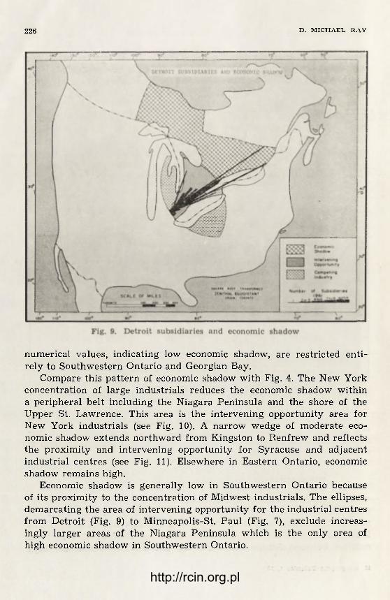
226 D. M I C H A E L . R A Y
numerical values, indicating low economic shadow, are restricted enti-rely to Southwestern Ontario and Georgian Bay.
Compare this pattern of economic shadow with Fig. 4. The New York concentration of large industrials reduces the economic shadow within a peripheral belt including the Niagara Peninsula and the shore of the Upper St. Lawrence. This area is the intervening opportunity area for New York industrials (see Fig. 10). A narrow wedge of moderate eco-nomic shadow extends northward from Kingston to Renfrew and reflects the proximity and intervening opportunity for Syracuse and adjacent industrial centres (see Fig. 11). Elsewhere in Eastern Ontario, economic shadow remains high.
Economic shadow is generally low in Southwestern Ontario because of its proximity to the concentration of Midwest industrials. The ellipses, demarcating the area of intervening opportunity for the industrial centres from Detroit (Fig. 9) to Minneapolis-St. Paul (Fig. 7), exclude increas-ingly larger areas of the Niagara Peninsula which is the only area of high economic shadow in Southwestern Ontario.
http://rcin.org.pl
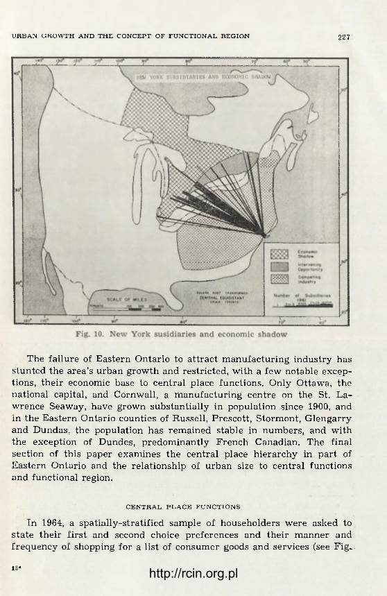
U R B A N G R O W T H A N D THE CONCEPT OF F U N C T I O N A L REGION 227
The failure of Eastern Ontario to attract manufacturing industry has stunted the area's urban growth and restricted, with a few notable excep-tions, their economic base to central place functions. Only Ottawa, the national capital, and Cornwall, a manufacturing centre on the St. La-wrence Seaway, have grown substantially in population since 1900, and in the Eastern Ontario counties of Russell, Prescott, Stormont, Glengarry and Dundas, the population has remained stable in numbers, and with the exception of Dundes, predominantly French Canadian. The final section of this paper examines the central place hierarchy in part of Eastern Ontario and the relationship of urban size to central functions and functional region.
C E N T R A L P L A C E F U N C T I O N S
In 1964, a spatially-stratified sample of householders were asked to state their first and second choice preferences and their manner and frequency of shopping for a list of consumer goods and services (see Fig_
14* http://rcin.org.pl

228 D. MICHAEL. R A Y
14). Mother tongue was recorded in order to determine cultural dif-ferences in consumer travel behaviour 62. The first choice shopping pat-terns for rural fa rm families have been mapped by drawing desire lines from place of residence direct to the place providing each service. These maps are ordered from hamlet-level to regional-capital level services to stress the relationship between level of service and size of functional region.
F O O D S E R V I C E S : F I G U R E 15
Food services are a hamlet-level function offered by all central places. A symmetry in the desire line pattern emerges f rom consistent
62 Robert A. Murdie, Cultural Differences in Consumer Travel, Economic Geo-graphy, Vol. 41. July 1965, pp. 211—233. Murdie finds significant differences in the consumer travel behaviour between Old Order Mennonites and „modern" Cana-dians in Waterloo and Wellington Counties of Southwestern Ontario for traditio-nal goods (auto and harness repair, food, clothing, yard goods and shoes).
http://rcin.org.pl

J J R B A N G R O W T H A N D THE CONCEPT OF F U N C T I O N A L REGION 229
consumer travel to the closest centre. The few exceptional cases, where consumers ignore an intervening opportunity, are explained by multi--purpose travel behaviour, or by cultural differences, with some French Canadian farmers preferring a French Canadian central place to a closer English centre. The perimeters of the desire lines delimit the functional regions and their length reveals the range of the good. The range of the good for food purchases is under three miles, and the maximum profit area that can be commanded by a centre for this service is very small. In a few cases, such as Limoges and Embrun, and St.-Rose-de-Prescott and St.-Isidore-de-Prescott, a small functional regions forms an enclave within a larger area. These smaller centres are candidates for early drop--out in the inter-urban competition to provide central functions.
A U T O R E P A I R S E R V I C E S : F I G U R E 16
Note the similarity between pattern of functional regions for food and auto repair services. This service is also considered hamlet-level, although half the hamlets fail to offer it and have their entire region absorbed by the closest larger central place. Such failures generally reflect proximity
http://rcin.org.pl

230 D. M I C H A E L . R A Y
Fig. 13. Eastern Ontario: population distribution
to a larger centre. For example, Inkerman fails to offer auto repair ser-vices and its region is absorbed by Winchester. The Limoges region is, however, served by Lemieux for auto repair, the only service provided by Lemieux. For all other services, it forms a part of the Embrun region. ; In a few exceptional cases, services may survive in a central place despite proximity to a competing centre. Winchester and Chesterville both offer food and auto repair services even though their proximity truncates their functional regions. This conflict between the two centres
http://rcin.org.pl
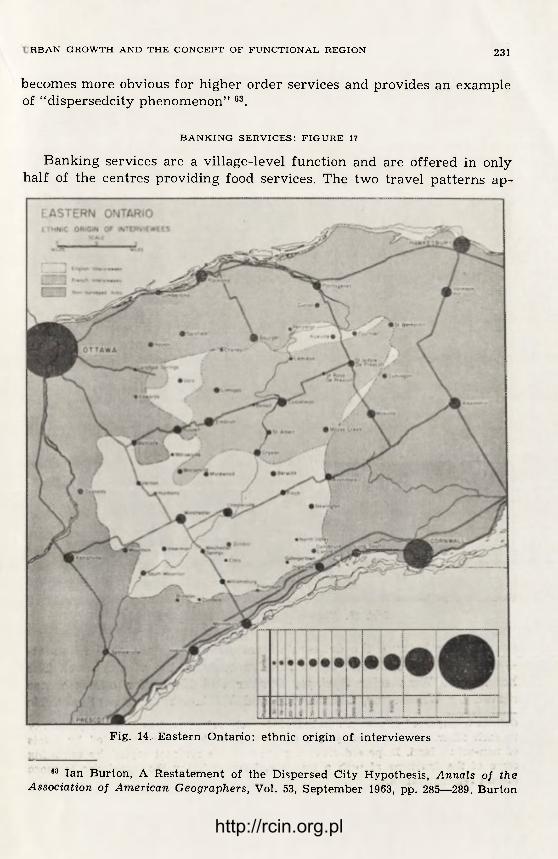
J J R B A N G R O W T H A N D THE CONCEPT OF F U N C T I O N A L REGION 231
becomes more obvious for higher order services and provides an example of "dispersedcity phenomenon" 63.
B A N K I N G S E R V I C E S : F I G U R E 17
Banking services are a village-level function and are offered in only half of the centres providing food services. The two travel patterns ap-
Fig. 14. Eastern Ontario: ethnic origin of interviewers
63 Ian Burton, A Restatement of the Dispersed City Hypothesis, Annals of the Association of American Geographers, Vol. 53, September 1963, pp. 285—289. Burton
http://rcin.org.pl

232 D. M I C H A E L . R A Y
Fig. 15. Eastern Ontario: food services
pear similar because the drop-outs form enclave regions at the hamlet--service level and do not cause re-alignments at the village level. The hamlets of Winchester Springs, Dunbar and Elma, for example, are served by Winchester, Chesterville and Williamsburg respectively. No
defines a dispersed city as a number of discrete urban centres in close proximity to each other and functionally interrelated, although usually separated by tracts of non-urban land. Dispersed cities replace a single regional capital by capturing some of the functions of such a centre and surrendering the remainder to more distant regional capitals.
http://rcin.org.pl

J J R B A N G R O W T H A N D THE CONCEPT OF F U N C T I O N A L REGION 233
Fig. 16. Eastern Ontario: auto repair services
cultural preferences are apparent. French Canadians living closer to Russell than to Embrun use the Bank of Nova Scotia at Russell ra ther than the Caisse Populaire at Embrun, for example.
M E D I C A L A N D L E G A L S E R V I C E S : F I G U R E S 18 A N D 19
Medical and legal services are town-level services; the village of South Mountain and its region, for example, are served by Winchester. Higher order services aire used less frequently than low order services
http://rcin.org.pl
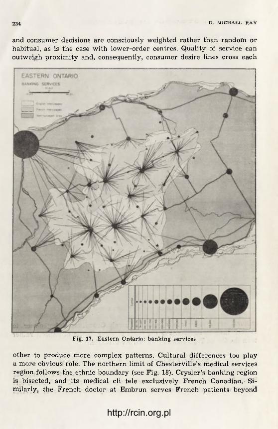
234 D. M I C H A E L . R A Y
and consumer decisions are consciously weighted rather than random or habitual, as is the case with lower-order centres. Quality of service can outweigh proximity and, consequently, consumer desire lines cross each
Fig. 17. Eastern Ontario: banking services
other to produce more complex patterns. Cultural differences too play a more obvious role. The northern limit of Chesterville's medical services region follows the ethnic boundary (see Fig. 18). Crysler's banking region is bisected, and its medical cli tele exclusively French Canadian. Si-milarly, the French doctor at Embrun serves French patients beyond
http://rcin.org.pl
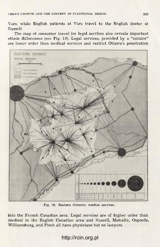
J J R B A N G R O W T H A N D T H E C O N C E P T OF F U N C T I O N A L R E G I O N 235
Vars, while English patients at Vars travel to the English doctor at Russell.
The map of consumer travel for legal services also reveals important ethnic differences (see Fig. 19). Legal services, provided by a "notaire" are lower order than medical services and restrict Ottawa's penetration
Fig. 18. Eastern Ontario: medica services
into the French Canadian area. Legal services are of higher order than medical in the English Canadian area and Russell, Metcalfe, Osgoode, Williamsburg, and Finch all have physicians but no lawyers.
http://rcin.org.pl

236 D. MICHAEL. R A Y
D E N T A L S E R V I C E S : F I G U R E 20
Dental services are a city-level function. In the French Canadian area, Casselman alone has dental services; this is provided in the public school by the Hawkesbury dentist. Winchester and Chesterville both have larger functional regions which extend into the French ethnic area.
Fig. 19. Eastern Ontario: ega services
Casselman, Winchester and Chesterville are about equidistant from their competing centres, Ottawa and Cornwall, and just beyond the range of their effective competition.
http://rcin.org.pl

J J R B A N G R O W T H A N D T H E CONCEPT OF F U N C T I O N A L REGION 237
O P T I C A L S E R V I C E S : F I G U R E 21
The Ottawa and Cornwall functional regions meet for optical services which are a regional-capital function. The functional regions of Cassel-man, Winchester and Chesterville fall entirely within the Ottawa region. The pattern of areal functional organization is fully nested such that the region served by the regional-capital subdivides into city, town, village and hamlet subregions in turn 64. This nesting agrees with other empi-rical work.
64 A. K. Philbrick, Principles of Areal Functional Organization in Regional Human Geography, Economic Geography, Vol. 33, 1957, pp. 306—336.
http://rcin.org.pl
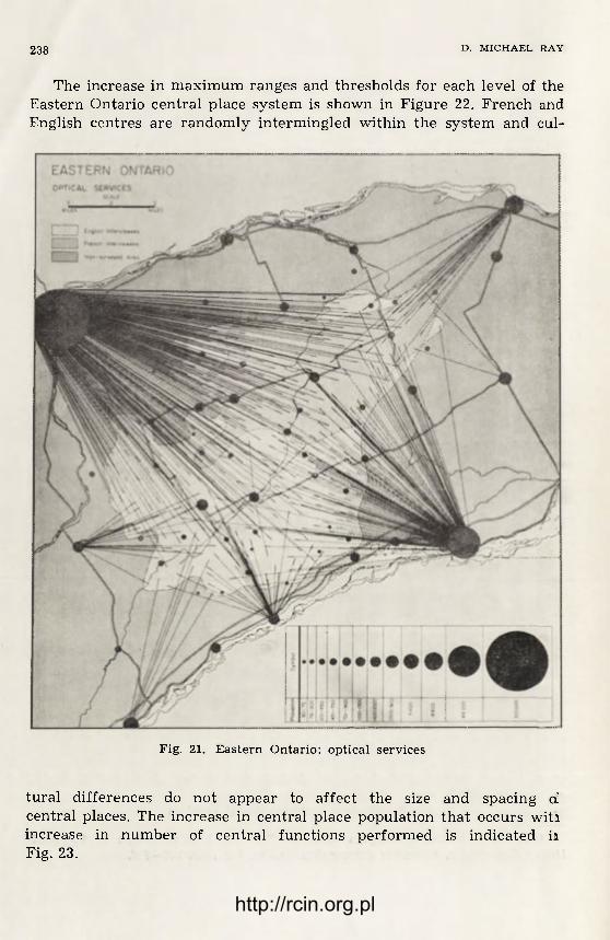
238 D. M I C H A E L . R A Y
The increase in maximum ranges and thresholds for each level of the Eastern Ontario central place system is shown in Figure 22. French and English centres are randomly intermingled within the system and cul-
Fig. 21. Eastern Ontario: optical services
tural differences do not appear to affect the size and spacing d central places. The increase in central place population that occurs witi increase in number of central functions performed is indicated ii Fig. 23.
http://rcin.org.pl

J J R B A N G R O W T H A N D T H E C O N C E P T OF F U N C T I O N A L R E G I O N 2 3 9
CONCLUSION
"Human activities are distributed over the national terr i tory in cer-tain rhythms and patterns which are neither arbitrary not the workings of chance. They result rather f rom the interpendencies that give form to economic space" 65. This paper has traced the interpendencies between geographic location, urban functions, functional regions and urban
R
Fig. 22. Range aod threshold graph foreastern Ontario
growth. It shows that one area, Eastern Ontario, has been unable to at-tract United States manufacturing subsidiaries because it is in the area of high economic shadow cast by Toronto, even though its geographic location, as measured by market potential, is otherwise favourable. The
85 Friedmann and Alonso, op. cit., p. 2.
http://rcin.org.pl
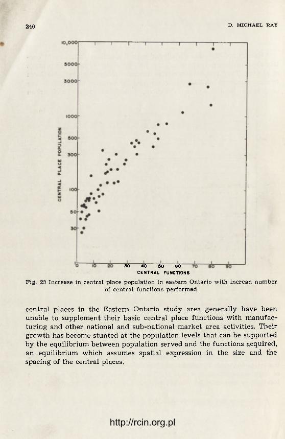
240 D. M I C H A E L . R A Y
30 40 50 60 CENTRAL FUNCTIONS
Fig. 23 Increase in central place population in eastern Ontario with increan number of central functions performed
central places in the Eastern Ontario study area generally have been unable to supplement their basic central place functions with manufac-turing and other national and sub-national market area activities. Their growth has become stunted at the population levels that can be supported by the equilibrium between population served and the functions acquired, an equilibrium which assumes spatial expression in the size and the spacing of the central places.
http://rcin.org.pl

http://rcin.org.pl

Cena i ł 56,—