ARTICLE

Spatial Variability of Annual Estimates of MethaneEmissions in a Phragmites Australis (Cav.) Trin. ex Steud.Dominated Restored Coastal Brackish Fen

Stefan Koch & Gerald Jurasinski & Franziska Koebsch &

Marian Koch & Stephan Glatzel

Received: 28 August 2013 /Accepted: 4 March 2014# Society of Wetland Scientists 2014

Abstract Methane is a major greenhouse gas with a globalwarming potential 25 times higher than carbon dioxide over a100 year time horizon. Determining annual emission esti-mates, usually specified for different vegetation types underparticular land use, requires the use of chamber measure-ments. These emission estimates may be strongly biased to-wards the lower or upper end by the spatial arrangement ofmeasurement spots in the ecosystem. Here, we analyze thespatial variability of annual methane emission estimates basedon non-steady state closed chamber measurements in pure andmixed stands of Phragmites australis (Cav.) Trin ex Steud. ina restored coastal brackish fen. Annual methane emissionestimates per measurement location vary largely between 46and 1,329 kg ha−1 a−1 CH4 but they do not differ significantlybetween pure and mixed stands of P. australis. Mantel testsshow a significant correlation of distances between spots andthe variation in methane emission estimates (p<0.05). Spatialcorrelation of water levels and annual methane emission esti-mates is not significant. Empirical variograms suggest thatvariance in annual methane emission estimates is not increas-ing with increasing spatial distance. However, spots that sharelarger distances may differ considerably in their annual meth-ane emission estimates. At the same time, spots that sharesmaller distances–though these exceed the distances commonto many closed chamber measurement setups–may differ lessin their annual methane emission estimates. Thus, a huge partof the natural variation in annual methane emissions in aparticular ecosystem or vegetation type may be missed whenusing the typical clustered arrangement of measurement loca-tions in closed chamber studies. Therefore, we suggest that

measurement locations should cover a wide spatial extent toimprove the reliability of annual emission estimates per veg-etation type and ecosystem, and that the number of measure-ment locations appropriate should be determined by pre-studies whenever possible.

Keywords CH4. Peatland . Spatial variation . Reed .

Greenhouse gas emissions . Shallow lake . Rewetting .

Restoration

Introduction

Methane (CH4) is an important greenhouse gas that signifi-cantly contributes to global warming with a radiative forcing2 5 t im e s h i g h e r t h a n c a r b o n d i o x i d e (CO2 )(Intergovernmental Panel of Climate Change 2007). Peatlandscover barely 3 % of the Earth’s land surface (Clymo 1987) butthey store up to one-third of the Earth’s soil carbon (Holden2005) and account for roughly 12 % of global CH4 emissions(Askaer et al. 2011). Although peatlands fix carbon dioxidefrom the atmosphere they are the most important naturalsource of atmospheric CH4 and have the highest carbondensity among all terrestrial ecosystems (Kayranli et al.2010). Therefore, peatlands can have a positive net radiativeforcing (Baird et al. 2010). For all that, quantifying globalCH4 budgets and identifying relevant processes mediatingCH4 release remains challenging.

A frequently used approach for estimating greenhouse gas(GHG) fluxes from peatlands is the non-steady state closedchamber method (Livingston and Hutchinson 1995). Wherepossible and feasible, closed chamber measurements of CH4

may be replaced by the micrometeorological eddy covariancetechnique that allows CH4 measurements over a wider spatialextent (Hendriks et al. 2010). The eddy covariance technique

S. Koch (*) :G. Jurasinski : F. Koebsch :M. Koch : S. GlatzelUniversität Rostock, Agrar- und Umweltwissenschaftliche Fakultät,Justus-von-Liebig-Weg 6, 18059 Rostock, Germanye-mail: stefan.koch4@uni-rostock.deURL: http://www.auf-loe.uni-rostock.de/en/staff/stefan-koch/

WetlandsDOI 10.1007/s13157-014-0528-z

provides numerous benefits compared to the closed chamberapproach in GHG measurements, such as quasi-continuouslymeasured time series of atmospheric CH4 concentration foranalysis of temporal variability (Teh et al. 2011), integrationover a large spatial scale, and an undisturbed measurement ofGHG fluxes. However, estimations of emission factors forspecific vegetation types—especially when they typicallycover only small patches—still require chamber based mea-surements. Commonly, the measurement locations for cham-ber measurements (“spots” in the following) are arranged inclusters and share distances of a few meters within one veg-etation type or land use unit (Askaer et al. 2011; Yamulki et al.2012; Beetz et al. 2013) mainly, to keep the effort manageable.Typically, rather few spatial replicates of these measurementsare used to reduce the effects of spatial variability on estimatedfluxes.

CH4 emissions often show large spatial variability(Hendriks et al. 2010). Spatial patterns in CH4 emissions areoften attributed to differences in ground water level (Mooreand Knowles 1990; Jungkunst and Fiedler 2007) and vegeta-tion composition (Joabsson et al. 1999; Ding et al. 2005;Butenhoff and Khalil 2007; Dias et al. 2010). Schrier-Uijlet al. (2010) found differences of 55 % between estimatedfluxes by chamber and eddy covariance measurements. Thesedifferences could be attributed to a disturbed microclimate inthe chamber headspace. Smith et al. (1994) stated, that cham-ber based measurements may give higher flux rates thanmicro-meteorologically measured fluxes due to the high spa-tial variability of CH4 exchange in peatlands, i.e. measurementlocations may have been positioned in areas with higher orlower fluxes. Hence, using the closed chamber approach andnot considering spatial variability in the arrangement of mea-surement spots may strongly influence annual emissionestimates.

Commonly, studies regarding spatial variability of CH4

emissions are restricted to simple statistical measures, in par-ticular mean values, standard deviations and the coefficient ofvariation (Schrier-Uijl et al. 2008; Hendriks et al. 2010; Zhaoet al. 2013). However, geostatistical methods like semi-variogram models—which describe the spatial dependenceof a random function—are more appropriate for quantifyingspatial variability (Lark 2002). The advantage of not neces-sarily using regular sampling grids has to be highlightedbecause of its importance in environmental sciences (Einax1995). Furthermore, these geostatistical methods can be usedfor the estimation of unsampled points and a discrete interpo-lation of measured variables using regression kriging (Henglet al. 2004).

Here, we analyze the spatial variability of CH4 emissions inan inundated rewetted coastal brackish fen in northeasternGermany focusing on Phragmites australis (Cav.) Trin. exSteud. dominated areas using geostatistical methods, particu-larly semi-variograms and theoretical semi-variogrammodels.

We hypothesize that (I) CH4 exchange exhibits highspatial variability in inundated peatlands as a result of di-verse environmental properties in the study area, (II) plantspecies composition controls spatial variability of CH4

emissions and, (III) plot selection and spatial arrangementof measurement spots are crucial for obtaining reliable emis-sion factors.

Material and Methods

Study Site and Setup

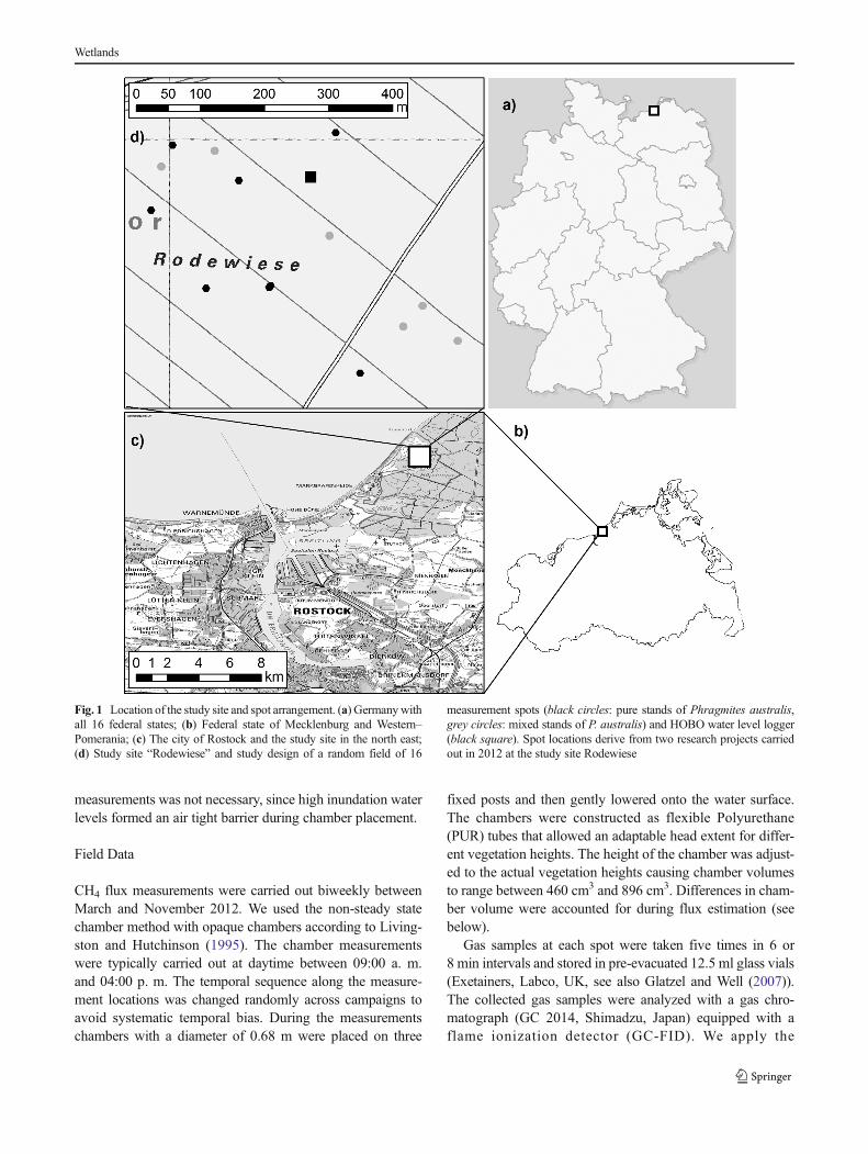
The study site Rodewiese is located in northeastern Germanyin the federal state of Mecklenburg Western-Pomerania(Fig. 1). It is a restored coastal brackish fen located 10 kmnortheast of the city of Rostock (54°12′ N, 12°10′ E) and ispart of the 493 ha large nature protection area “Heiligenseeund Hütelmoor”. The mean annual temperature is 9.1 °C witha total annual precipitation of 645 mm (reference period1981–2010, Koebsch et al. 2013).

The fen is separated from the Baltic Sea by a dune dikeinstalled in 1963 which increased fresh water supply. The areahad been intensively drained for grassland use since the 1970swith water levels down to 1.60 m below ground surface.Therefore, the peat in the upper soil horizons is weakly tostrongly decomposed (von Post decomposition values (vonPost 1922) ranged from H4 to H9 for the upper peat layers).Peat depths range between 1 and 3 mwith alternating layers ofsandy sediments as a result of flooding events (Koebsch et al.2013). For nature protection purposes first restoration mea-sures were taken in 1992 by closing the main ditch(Schoenfeld-Bockholdt et al. 2005). Almost 20 years later,in 2009 a ground sill was installed to permanently increase thewater level to or above ground surface. Since then, the fen ispermanently inundated with water levels up to 1.00 m aboveground surface.

In the past occasional storm surges caused waveovertopping of the dune dike and lead to flooding of the areawith brackish waters. This happened the last time in 1995.Dominant species are Common reed (P. australis), sedge spe-cies (Carex spp. L.), Sea-Club rush (Bolboschoenus maritimus(L.) Palla) and Softstem bulrush (Schoenoplectustabernaemontani (C. C. Gmel.) Palla).

We measured CH4 fluxes using a randomized samplingdesign of 16 measurement spots (Fig. 1). This provides fullindependence of each sample. Due to the incorporation of onecluster of three measurement locations that share distances ofabout 1 m, the distances between all possible pairs of mea-surement spots range between 1 m and 539 m. In order tominimize disturbance during chamber measurements board-walks were installed at each spot at least half a year beforemeasurements started. Installing collars for chamber

Wetlands

measurements was not necessary, since high inundation waterlevels formed an air tight barrier during chamber placement.

Field Data

CH4 flux measurements were carried out biweekly betweenMarch and November 2012. We used the non-steady statechamber method with opaque chambers according to Living-ston and Hutchinson (1995). The chamber measurementswere typically carried out at daytime between 09:00 a. m.and 04:00 p. m. The temporal sequence along the measure-ment locations was changed randomly across campaigns toavoid systematic temporal bias. During the measurementschambers with a diameter of 0.68 m were placed on three

fixed posts and then gently lowered onto the water surface.The chambers were constructed as flexible Polyurethane(PUR) tubes that allowed an adaptable head extent for differ-ent vegetation heights. The height of the chamber was adjust-ed to the actual vegetation heights causing chamber volumesto range between 460 cm3 and 896 cm3. Differences in cham-ber volume were accounted for during flux estimation (seebelow).

Gas samples at each spot were taken five times in 6 or8 min intervals and stored in pre-evacuated 12.5 ml glass vials(Exetainers, Labco, UK, see also Glatzel and Well (2007)).The collected gas samples were analyzed with a gas chro-matograph (GC 2014, Shimadzu, Japan) equipped with aflame ionization detector (GC-FID). We apply the

Fig. 1 Location of the study site and spot arrangement. (a) Germanywithall 16 federal states; (b) Federal state of Mecklenburg and Western–Pomerania; (c) The city of Rostock and the study site in the north east;(d) Study site “Rodewiese” and study design of a random field of 16

measurement spots (black circles: pure stands of Phragmites australis,grey circles: mixed stands of P. australis) and HOBO water level logger(black square). Spot locations derive from two research projects carriedout in 2012 at the study site Rodewiese

Wetlands

atmospheric sign convention, thus positive fluxes indicateemission of CH4 to the atmosphere whilst negative fluxesindicate uptake to the ecosystem.

Fluxes were estimated by the slope of the linear regressionof CH4 concentrations in the chamber headspace by using thestatistical computation software R (R Development CoreTeam 2012) and the package flux (Jurasinski et al. 2013).Flux measurements with regression curves and coefficientsof determination (R2) below 0.8 and normalized root meansquare (NRMSE) error above 0.2 were rejected. Regressioncurves without significant increase or decrease in headspaceCH4 concentration were defined to be zero fluxes. We did notapply any further outlier detection, since we measured veryhigh fluxes regularly. Checking all curves of the methaneconcentration change in the chamber headspace showed thatit is highly unlikely that ebullition fluxes occurred during ourmeasurements.

Annual emissions for each spot were estimated by linearinterpolation between daily fluxes and integrating those overtime using Monte-Carlo sampling with function auc.mc inpackage flux (Jurasinski et al. 2013, details in Koebsch et al.2013). This approach allows for estimating the error that isintroduced by temporal variation in sampling and by possiblymissing high/low fluxes during sampling. The functionauc.mc integrates the fluxes over the covered time periodmany times (here we used n=1,000), each time randomlyleaving out a specified number (lo=2) of measurements. Fromthe resulting distribution of emission estimates per spot wecalculated the mean, reflecting the best estimate, and thestandard deviation, providing an estimate for the asso-ciated uncertainty due to linear interpolation betweenmeasurement dates and to possible diurnal variation ofmethane fluxes. Diurnal variations in methane emissionsmay introduce some error into the analysis of spatialvariability, especially if the fluctuation cannot be ruledout using the obtained data, which is hard to achievewith chamber based measurements. However, Güntheret al. (2013) recently showed that diurnal variations ofmethane emissions do not influence annual emissionestimates significantly. Therefore, we base our analysison annual emission estimates.

Winter fluxes (November to February) were considered tobe negligible for annual balances due to climatic conditionsand ice cover on the open water table. Hence, the term annualemission in this study refers to CH4 emission estimates perspot derived from data that were recorded in the field fromMarch through October.

We measured water level continuously using a HOBOU20Water Level Data Logger (Onset, USA) within the study site(Fig. 1). The water observation tube and the data logger wereinstalled in May 2011. Water level data were averaged andtransferred to each spot by a 1 m Last Pulse laser scanningelevation model with relative vertical accuracy of a few

centimeters (obtained from the federal ministry of administra-tion Mecklenburg-Western Pomerania) that was acquired in2007 before flooding of the site. This was feasible because thearea was permanently inundated during our study. Plant spe-cies composition was recorded once in May 2012 by countingof species and estimating the cover of each species at thespots. The species cover estimates are treated as measures ofabundance in the following. The cover of P. australis rangesfrom 1 to 85 % across all measurements spots.

Statistical Analysis

Pure and mixed stands of P. australis were analysed forcorrelation between annual CH4 emission and inter-spot dis-tance. Pure vs. mixed stands were defined using the abun-dances of the accompanying species. If these were lower than5 %, the stands were defined as pure; if not, the stands weredefined as mixed. Accompanying species were Lemna minorL., Lemna triscula L. and Agrostis stolonifera L.

Mantel tests (Mantel 1967) were performed to evaluate therelationship of spatial distance matrices and the annual CH4

emission distance matrices. Dissimilarities of properties ofseveral locations and their spatial location were tested. Thedetection of spatial patterns in ecological data is known to bedifficult for small data sets. Therefore, we applied a random-ized Mantel test with a jackknife approach to test for theminimum number of measurement locations for spatial corre-lation of CH4 emissions and spot location.

The number of measurements required to estimate themeasured mean value of CH4 within a given error tolerancewas estimated by running 1,000 bootstrapping iterations ofrandomly chosen subsamples of the overall dataset startingwith a subsample size of n=1. The mean value across allsubsamples was calculated, repeating this procedure for allconsecutive subsample sizes of n=1+i, with i=1…n-1. Therequired number of observations was determined if the chosentarget value was estimated by the mean of all subsamples witha 95 % probability.

Geostatistical Analysis

Spatial auto-correlation of CH4 emission was calculated usingsemi-variograms and the semi-variance γ(h)

γ hð Þ ¼ 1

2n hð ÞXn hð Þ

i¼1Z xið Þ−Z xj

� �� �2 ðIÞ

where xi and xj are the locations of two measurement spots,n(h) is the set of all pairwise Euclidean distances and Z is thevalue of the estimated annual CH4 emission at the referredlocation. These empirical semi-variances γ(h) were fitted tothree different theoretical semi-variogram models. Here,we used the spherical (IIa and IIb), the wave (III) and

Wetlands

the linear model. These models were fitted using thefollowing equations:

γ hð Þ ¼ c0 þ c⋅3h

2a−

h3

2a3

� �; f or 0 < h≤a ðIIaÞ

γ hð Þ ¼ c0 þ c; f or h > a ðIIbÞ

γ hð Þ ¼ c0 þ c⋅ 1−sin

h

a

� �

h

a

0BB@

1CCA ðIIIÞ

where h is the Euclidean distance, c0 is the nugget, c0+c is thesill, and a is the range of the semi-variogram. The theoreticalvariogram models were compared and validated by the min-imized sum of squares.

We calculated semi-variances using normalized annualCH4 emission estimates. Normalization was done by dividingannual CH4 emission estimates by the maximum annual emis-sion estimate. This approach decreases the range of valuesboth in the generic data and the calculated semi-variances andtherefore optimizes comparability and interpretability of theresults. An additional transformation of the data was notnecessary due to normally distributed annual emissionestimates.

Results

CH4 Fluxes and Annual Emissions Estimates

In total we recorded 269 chamber measurements within8 months. 87 estimated fluxes (30 %) were rejected due toinsufficient quality parameters. Of the remaining fluxes(n=182), 157 fluxes were estimated as positive, 25 asnegative. Minimum and maximum CH4 fluxes were −8.2 and60.8 mg m−2 h−1CH4. On average the mean CH4 flux(± standard deviation) was 12.4±13.7 mg m-2 h-1 CH4

across all spots and P. australis abundances.Average CH4 flux was 17.6±16.8 in pure (n=59) and

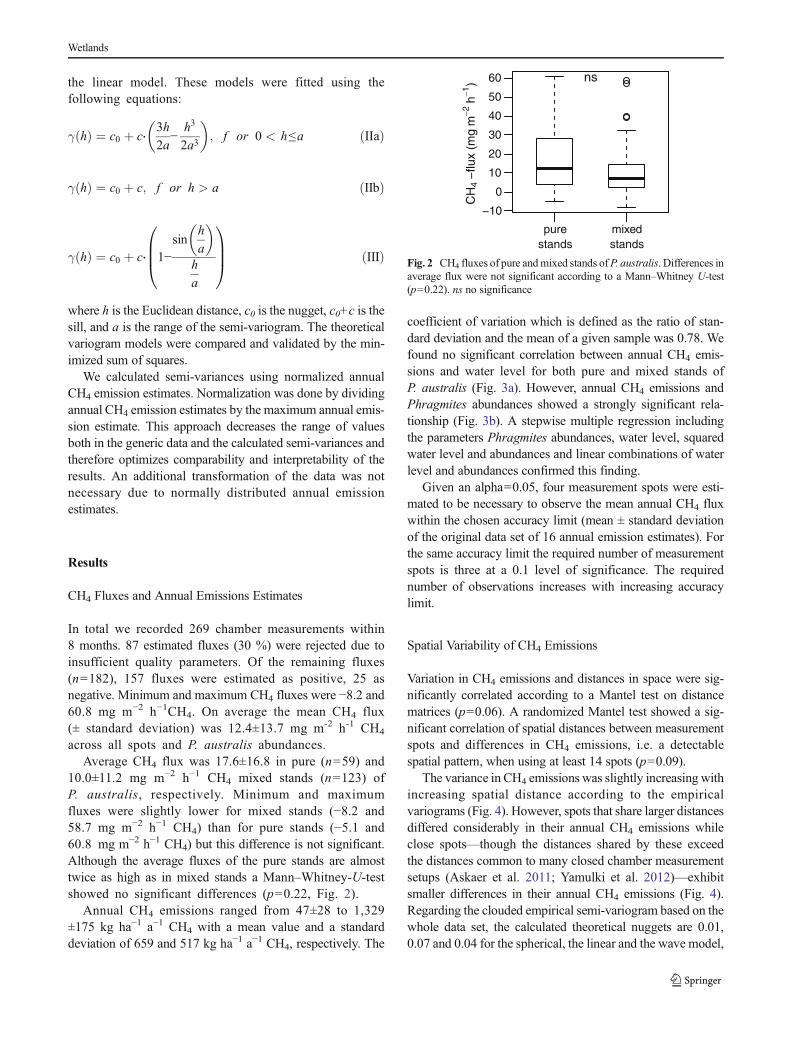
10.0±11.2 mg m−2 h−1 CH4 mixed stands (n=123) ofP. australis, respectively. Minimum and maximumfluxes were slightly lower for mixed stands (−8.2 and58.7 mg m−2 h−1 CH4) than for pure stands (−5.1 and60.8 mg m−2 h−1 CH4) but this difference is not significant.Although the average fluxes of the pure stands are almosttwice as high as in mixed stands a Mann–Whitney-U-testshowed no significant differences (p=0.22, Fig. 2).

Annual CH4 emissions ranged from 47±28 to 1,329±175 kg ha−1 a−1 CH4 with a mean value and a standarddeviation of 659 and 517 kg ha−1 a−1 CH4, respectively. The

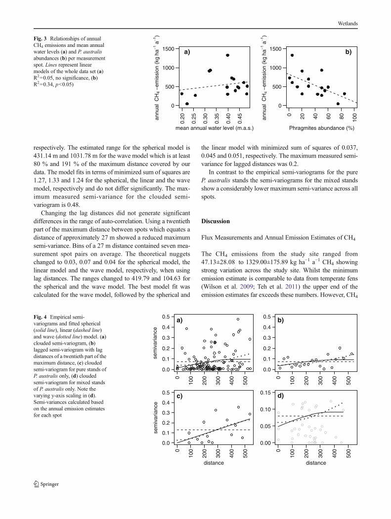
coefficient of variation which is defined as the ratio of stan-dard deviation and the mean of a given sample was 0.78. Wefound no significant correlation between annual CH4 emis-sions and water level for both pure and mixed stands ofP. australis (Fig. 3a). However, annual CH4 emissions andPhragmites abundances showed a strongly significant rela-tionship (Fig. 3b). A stepwise multiple regression includingthe parameters Phragmites abundances, water level, squaredwater level and abundances and linear combinations of waterlevel and abundances confirmed this finding.

Given an alpha=0.05, four measurement spots were esti-mated to be necessary to observe the mean annual CH4 fluxwithin the chosen accuracy limit (mean ± standard deviationof the original data set of 16 annual emission estimates). Forthe same accuracy limit the required number of measurementspots is three at a 0.1 level of significance. The requirednumber of observations increases with increasing accuracylimit.

Spatial Variability of CH4 Emissions

Variation in CH4 emissions and distances in space were sig-nificantly correlated according to a Mantel test on distancematrices (p=0.06). A randomized Mantel test showed a sig-nificant correlation of spatial distances between measurementspots and differences in CH4 emissions, i.e. a detectablespatial pattern, when using at least 14 spots (p=0.09).

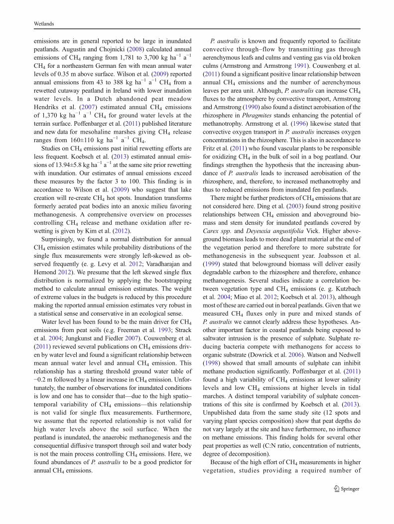
The variance in CH4 emissions was slightly increasing withincreasing spatial distance according to the empiricalvariograms (Fig. 4). However, spots that share larger distancesdiffered considerably in their annual CH4 emissions whileclose spots—though the distances shared by these exceedthe distances common to many closed chamber measurementsetups (Askaer et al. 2011; Yamulki et al. 2012)—exhibitsmaller differences in their annual CH4 emissions (Fig. 4).Regarding the clouded empirical semi-variogram based on thewhole data set, the calculated theoretical nuggets are 0.01,0.07 and 0.04 for the spherical, the linear and the wave model,

purestands

mixedstands

−10

0

10

20

30

40

50

60

CH

4−

flux

(mg

m2

h1) ns

Fig. 2 CH4 fluxes of pure andmixed stands ofP. australis. Differences inaverage flux were not significant according to a Mann–Whitney U-test(p=0.22). ns no significance

Wetlands

respectively. The estimated range for the spherical model is431.14 m and 1031.78 m for the wave model which is at least80 % and 191 % of the maximum distance covered by ourdata. The model fits in terms of minimized sum of squares are1.27, 1.33 and 1.24 for the spherical, the linear and the wavemodel, respectively and do not differ significantly. The max-imum measured semi-variance for the clouded semi-variogram is 0.48.

Changing the lag distances did not generate significantdifferences in the range of auto-correlation. Using a twentiethpart of the maximum distance between spots which equates adistance of approximately 27 m showed a reduced maximumsemi-variance. Bins of a 27 m distance contained seven mea-surement spot pairs on average. The theoretical nuggetschanged to 0.03, 0.07 and 0.04 for the spherical model, thelinear model and the wave model, respectively, when usinglag distances. The ranges changed to 419.79 and 104.63 forthe spherical and the wave model. The best model fit wascalculated for the wave model, followed by the spherical and

the linear model with minimized sum of squares of 0.037,0.045 and 0.051, respectively. The maximum measured semi-variance for lagged distances was 0.2.

In contrast to the empirical semi-variograms for the pureP. australis stands the semi-variograms for the mixed standsshow a considerably lower maximum semi-variance across allspots.

Discussion

Flux Measurements and Annual Emission Estimates of CH4

The CH4 emissions from the study site ranged from47.13±28.08 to 1329.00±175.89 kg ha−1 a−1 CH4 showingstrong variation across the study site. Whilst the minimumemission estimate is comparable to data from temperate fens(Wilson et al. 2009; Teh et al. 2011) the upper end of theemission estimates far exceeds these numbers. However, CH4

0.20

0.25

0.30

0.35

0.40

0.45

0

500

1000

1500

mean annual water level (m.a.s.)

annu

al C

H4

−em

issi

on (

kgha

1a

1)

a)

0 20 40 60 80 100

0

500

1000

1500

Phragmites abundance (%)

annu

al C

H4

−em

issi

on (

kgha

1a

1)

b)

Fig. 3 Relationships of annualCH4 emissions and mean annualwater levels (a) and P. australisabundances (b) per measurementspot. Lines represent linearmodels of the whole data set (a)R2=0.05, no significance, (b)R2=0.34, p<0.05)

0

100

200

300

400

500

0.0

0.1

0.2

0.3

0.4

0.5

sem

ivar

ianc

e

a)

0

100

200

300

400

500

0.0

0.1

0.2

0.3

0.4

0.5 b)

0

100

200

300

400

500

0.0

0.1

0.2

0.3

0.4

0.5

distance

sem

ivar

ianc

e

c)

0

100

200

300

400

500

0.00

0.05

0.10

0.15

distance

d)

Fig. 4 Empirical semi-variograms and fitted spherical(solid line), linear (dashed line)and wave (dotted line) model. (a)clouded semi-variogram, (b)lagged semi-variogram with lagdistances of a twentieth part of themaximum distance, (c) cloudedsemi-variogram for pure stands ofP. australis only, (d) cloudedsemi-variogram for mixed standsof P. australis only. Note thevarying y-axis scaling in (d).Semi-variances calculated basedon the annual emission estimatesfor each spot

Wetlands

emissions are in general reported to be large in inundatedpeatlands. Augustin and Chojnicki (2008) calculated annualemissions of CH4 ranging from 1,781 to 3,700 kg ha−1 a−1

CH4 for a northeastern German fen with mean annual waterlevels of 0.35 m above surface. Wilson et al. (2009) reportedannual emissions from 43 to 388 kg ha−1 a−1 CH4 from arewetted cutaway peatland in Ireland with lower inundationwater levels. In a Dutch abandoned peat meadowHendriks et al. (2007) estimated annual CH4 emissionsof 1,370 kg ha−1 a−1 CH4 for ground water levels at theterrain surface. Poffenbarger et al. (2011) published literatureand new data for mesohaline marshes giving CH4 releaseranges from 160±110 kg ha−1 a−1 CH4.

Studies on CH4 emissions past initial rewetting efforts areless frequent. Koebsch et al. (2013) estimated annual emis-sions of 13.94±5.8 kg ha−1 a−1 at the same site prior rewettingwith inundation. Our estimates of annual emissions exceedthese measures by the factor 3 to 100. This finding is inaccordance to Wilson et al. (2009) who suggest that lakecreation will re-create CH4 hot spots. Inundation transformsformerly aerated peat bodies into an anoxic milieu favoringmethanogenesis. A comprehensive overview on processescontrolling CH4 release and methane oxidation after re-wetting is given by Kim et al. (2012).

Surprisingly, we found a normal distribution for annualCH4 emission estimates while probability distributions of thesingle flux measurements were strongly left-skewed as ob-served frequently (e. g. Levy et al. 2012; Varadharajan andHemond 2012). We presume that the left skewed single fluxdistribution is normalized by applying the bootstrappingmethod to calculate annual emission estimates. The weightof extreme values in the budgets is reduced by this proceduremaking the reported annual emission estimates very robust ina statistical sense and conservative in an ecological sense.

Water level has been found to be the main driver for CH4

emissions from peat soils (e.g. Freeman et al. 1993; Stracket al. 2004; Jungkunst and Fiedler 2007). Couwenberg et al.(2011) reviewed several publications on CH4 emissions driv-en by water level and found a significant relationship betweenmean annual water level and annual CH4 emission. Thisrelationship has a starting threshold ground water table of−0.2 m followed by a linear increase in CH4 emission. Unfor-tunately, the number of observations for inundated conditionsis low and one has to consider that—due to the high spatio–temporal variability of CH4 emissions—this relationshipis not valid for single flux measurements. Furthermore,we assume that the reported relationship is not valid forhigh water levels above the soil surface. When thepeatland is inundated, the anaerobic methanogenesis and theconsequential diffusive transport through soil and water bodyis not the main process controlling CH4 emissions. Here, wefound abundances of P. australis to be a good predictor forannual CH4 emissions.

P. australis is known and frequently reported to facilitateconvective through–flow by transmitting gas throughaerenchymous leafs and culms and venting gas via old brokenculms (Armstrong and Armstrong 1991). Couwenberg et al.(2011) found a significant positive linear relationship betweenannual CH4 emissions and the number of aerenchymousleaves per area unit. Although, P. australis can increase CH4

fluxes to the atmosphere by convective transport, Armstrongand Armstrong (1990) also found a distinct aerobisation of therhizosphere in Phragmites stands enhancing the potential ofmethanotrophy. Armstrong et al. (1996) likewise stated thatconvective oxygen transport in P. australis increases oxygenconcentrations in the rhizosphere. This is also in accordance toFritz et al. (2011) who found vascular plants to be responsiblefor oxidizing CH4 in the bulk of soil in a bog peatland. Ourfindings strengthen the hypothesis that the increasing abun-dance of P. australis leads to increased aerobisation of therhizosphere, and, therefore, to increased methanotrophy andthus to reduced emissions from inundated fen peatlands.

There might be further predictors of CH4 emissions that arenot considered here. Ding et al. (2003) found strong positiverelationships between CH4 emission and aboveground bio-mass and stem density for inundated peatlands covered byCarex spp. and Deyeuxia angustifolia Vick. Higher above-ground biomass leads to more dead plant material at the end ofthe vegetation period and therefore to more substrate formethanogenesis in the subsequent year. Joabsson et al.(1999) stated that belowground biomass will deliver easilydegradable carbon to the rhizosphere and therefore, enhancemethanogenesis. Several studies indicate a correlation be-tween vegetation type and CH4 emissions (e. g. Kutzbachet al. 2004; Miao et al. 2012; Koebsch et al. 2013), althoughmost of these are carried out in boreal peatlands. Given that wemeasured CH4 fluxes only in pure and mixed stands ofP. australis we cannot clearly address these hypotheses. An-other important factor in coastal peatlands being exposed tosaltwater intrusion is the presence of sulphate. Sulphate re-ducing bacteria compete with methanogens for access toorganic substrate (Dowrick et al. 2006). Watson and Nedwell(1998) showed that small amounts of sulphate can inhibitmethane production significantly. Poffenbarger et al. (2011)found a high variability of CH4 emissions at lower salinitylevels and low CH4 emissions at higher levels in tidalmarches. A distinct temporal variability of sulphate concen-trations of this site is confirmed by Koebsch et al. (2013).Unpublished data from the same study site (12 spots andvarying plant species composition) show that peat depths donot vary largely at the site and have furthermore, no influenceon methane emissions. This finding holds for several otherpeat properties as well (C:N ratio, concentration of nutrients,degree of decomposition).

Because of the high effort of CH4 measurements in highervegetation, studies providing a required number of

Wetlands

measurement points in space cannot be found. A commonlyused approach in chamber measurements is the use of two orthree direct replicates in a spatial cluster unit (Askaer et al.2011; Sha et al. 2011; Schäfer et al. 2012; Yamulki et al.2012). Typically these units are called plots and are thoughtto be relatively homogenous in vegetation and environment.However, vicinity in space does not necessarily lead to similarenvironmental conditions in all aspects. Here, we did notprescribe in advance any plots. Instead the measurement lo-cations were distributed widely across the study site. With thissetup we found a minimum of four measurement spots to benecessary to estimate the given mean value (that is derivedusing data of all 16 measurement locations) ± standard devi-ation at a 0.05 level of significance. Since the application offour measurement spots gave us the mean value ± standarddeviation–which still means an uncertainty of up to 80 %–alower number of measurement locations will create largeuncertainties and deficient emission estimates. So we presumethat in our particular ecosystem a number of four measure-ment spots is the minimum number of spots that can be usedfor determining annual emission estimates. A higher numberof spots is preferable but limited funds and project time willhamper the implementation of this approach. Herbst et al.(2009) found a mean number of measurement points of 31for bare soil respiration necessary to estimate the mean valuewith a level of significance of 0.125. A comparison seemsdifficult, since bare soil respiration is controlled by otherprocesses than CH4 release from convective plants.

Spatial Variability of Annual Estimates of CH4 Emissions

The knowledge on spatial variability in a given ecosystem iscrucial for setting up experimental designs and for obtainingreliable annual emission estimates and furthermore to reducebias caused by spatial patterns in CH4 fluxes (Imer et al.2013). Although there are many studies on spatial variability(Schrier-Uijl et al. 2008; Hendriks et al. 2010; Zhao et al.2013), the number of studies using geostatistical approachesfor quantifying spatial variability of CH4 emissions is low(e. g. Imer et al. 2013). Studies regarding the spatial variabilityof ecosystem respiration in terms of geostatistical measuresare more numerous (Herbst et al. 2009; Jordan et al. 2009)since measurements of bare soil respiration are technicallysimpler and need less financial efforts.

The Mantel test can be used as a first proxy of spatialcorrelation based on distance matrices (closeness) by the useof Euclidean distances and an underlying normal distributionof the raw data (Dutilleul et al. 2000). These modificationspartly outweigh its imprecise estimation of the proportion ofthe original data variation explained by the spatial structures(Legendre and Fortin 2010).

In our study, the spatial variability for both P. australis pureand mixed stands and across all spots was high. The linear

model showed the largest auto-correlation, while auto-correlation for the spherical and the wave model was lowand medium, respectively. The semi-variances for our dataset of P. australis pure stands were higher than for mixedstands due to an overall higher range of annual CH4 emissionestimates in pure stands while containing fewer data points atthe same time.

A high spatial auto-correlation implies that the measure-ments of each individual chamber are not randomly distribut-ed in space (Imer et al. 2013). The absence of a sill in theermpirical semi-variograms is an indicator for trended data.We found no spatial trend for both pure (p=0.38) and mixed(p=0.18) stands of P. australis and directional semi-variograms show a similar behavior for each direction (datanot shown). Imer et al. (2013) state, that an erratic behavior ofthe empirical semi-variogram can indicate that CH4 emissionsrespond to processes acting on different spatial scales.

Based on our findings–using the spherical semi-variogrammodel–we recommend that the use of at least four measure-ment spots that are at least about 400 m apart from each otherwill deliver the best emission estimates not plagued by auto-correlation.

Despite the spatial aspect, temporal variability plays animportant role in assessing variability of methane emissions.Diurnal patterns in CH4 fluxes are observed frequently fordifferent wetland ecosystems (Kumar and Viyol 2009; Longet al. 2009). Also often a distinct seasonality is reported(Hendriks et al. 2010; Imer et al. 2013). We did not addressquestions of diurnal and annual temporal patterns because ourfocus is on the spatial variability of annual emission estimates.Since these are obtained with a Monte Carlo sampling proce-dure that acknowledges temporal uncertainty they are robustestimates of the annual emission that should not be biased dueto temporal variation.

Summary and Conclusion

We found a high spatial variability of chamber based CH4

emissions although we restricted our analysis to P. australisstands in a coastal rewetted fen. This suggests that small scaleprocesses that vary largely within ecosystems may be respon-sible for the high spatial variability. Further, our results sug-gest, that in fen ecosystems dominated by emergent macro-phytes, P. australis abundances seem to be a fair predictor forannual CH4 emissions but in a direction quite unexpected inadvance, i.e. that emissions increase with decreasingP. australis cover. In our study CH4 emissions showed noresponse to mean annual water level which may be due to theinundated conditions at our site and to the fact that we there-fore covered only a part of the water level gradient.

In our specific system we would have been able to obtain amean annual emission estimate within the set limits (standard

Wetlands

deviation around the mean) and tested against a significancelevel of 0.05 with 4 sampling locations. This still means thatthe reported value could deviate to as much as 80 % from themean we report based on 16 measurement locations. We wereonly able to derive this number because we hadmore locationssampled. Therefore, we recommend—despite ever-decreasingfunds and project time—to carry out pre-studies wheneverpossible to determine the appropriate number of samplinglocations for chamber based methane exchangemeasurementsfor the ecosystem and vegetation type under study.

Pre-studies, featuring a sequence of measurement cam-paigns, may best be carried out—at least in temperate andboreal systems—in the second part of the growing seasonprior to the start of the real measurements. During this timeof the year substrate supply and temperatures are both high,which typically leads to relatively high methane exchangerates. Therefore, this part of the year contributes a consider-able share of the annual emission estimate in temperate andboreal ecosystems and variation due to location in methaneemission estimates per time period—driven by whatever var-iables—should be most pronounced then. Such pre-studiesmay allow the assessment of spatial variance of methaneemissions to find the minimum number of measurement spotsrequired with defensible effort.

Based on our finding that variability between measurementlocations can be high at small and large distances betweenthem, we recommend the distribution of measurement spotsover a wide spatial extend and a wide range of characteristicsof the vegetation type being explored. We think that thisapproach can increase the quality of emission factors andshould therefore be promoted for future chamber based studiesof methane emissions whenever possible.

Acknowledgments This study was funded by the projects “COMTESS –sustainable land management: Trede-offs in ecosystem services” (funded bythe Federal Ministry of Education and Research Germany (BMBF),Framework programme “Research for Sustainable Development”(FONA)). Parts of the studywere funded by theGerman Science Foundation(DFG, JU 2780/4-1).

References

Armstrong J, Armstrong W (1990) Light-enhanced convectivethroughflow increases oxygenation in rhizomes and rhizosphere ofPhragmites australis (Cav.) Trin. Ex Steud. New Phytologist 114:121–128

Armstrong J, ArmstrongW (1991) A convective through-flow of gases inPhragmites australis (Cav.) Trin ex. Steud. Aquatic Botany 39:75–88

Armstrong J, Armstrong W, Beckett PM, Halder JE, Lythe S, Holt R,Sinclair A (1996) Pathways of aeration and the mechanisms andbeneficial effects of humidity- and Venturi-induced convections inPhragmites australis (Cav.)Trin. ex Steud. Aquatic Botany 54:177–197

Askaer L, Elberling B, Friborg T, Jørgensen CJ, Hansen BU (2011) Plant-mediated CH4 transport and C gas dynamics quantified in-situ in aPhalaris arundinacea-dominant wetland. Plant and Soil 343(1–2):287–301

Augustin J, Chojnicki B (2008) Austausch von klimarelevantenSpurengasen, Klimawirkung und Kohlenstoffdynamik in den erstenJahren nach der Wiedervernässung von degradiertemNiedermoorgrünland. In: Gelbrecht J, Zak D, Augustin J (eds)Phosphor- und Kohlenstoff-Dynamik und Vegetationsentwicklungin wiedervernässten Mooren des Peenetals in Mecklenburg-Vorpommern. Leibniz-Institut für Gewässerökologie undBinnenfischerei, Berlin, pp 50–67

Baird AJ, Stamp I, Heppell CM, Green SM (2010) CH4 flux frompeatlands: a new measurement method. Ecohydrology 33:360–367

Beetz S, Liebersbach H, Glatzel S, Jurasinski G, Buczko U, Höper H(2013) Effects of land use intensity on the full greenhouse gasbalance in an Atlantic peat bog. Biogeosciences 10(2):1067–1082

Butenhoff CL, Khalil MAK (2007) Global methane emissions fromterrestrial plants. Environmental Science and Technology 41(11):4032–4037

Clymo RS (1987) The ecology of peatlands. Science Progress (Oxford)71:593–614

Couwenberg J, Thiele A, Tanneberger F, Augustin J, Bärisch S, DubovikD, Liashchynskaya N, Michaelis D, Minke M, Skuratovich A,Joosten H (2011) Assessing greenhouse gas emissions frompeatlands using vegetation as a proxy. Hydrobiologia 674(1):67–89

Dias ATC, Hoorens B, Logtestijn RSP, Vermaat JE, Aerts R (2010) Plantspecies composition can be used as a proxy to predict methaneemissions in peatland ecosystems after land-use changes.Ecosystems 13(4):526–538

Ding W, Cai Z, Tsuruta H, Li X (2003) Key factors affecting spatialvariation of methane emissions from freshwater marshes.Chemosphere 51:167–173

Ding W, Cai Z, Tsuruta H (2005) Plant species effects on methaneemissions from freshwater marshes. Atmospheric Environment39(18):3199–3207

Dowrick DJ, Freeman C, Lock MA, Reynolds B (2006) Sulphate reduc-tion and the suppression of peatland methane emissions followingsummer drought. Geoderma 132(3–4):384–390

Dutilleul P, Stockwell D, Frigon D, Legendre P (2000) The Mantel testversus Pearson’s correlation analysis: assessment of the differencesfor biological and environmental studies. Journal of Agricultural,Biological, and Environmental Statistics 5(2):131–150

Einax JSU (1995) Geostatistical investigations of polluted soils.Fresenius' Journal of Analytical Chemistry 351:48–53

Freeman C, Lock MA, Reynolds B (1993) Fluxes of CO2, CH4 and N2Ofrom a Welsh peatland following simulation of water table draw-down: potential feedback to climatic change. Biogeochemistry 19:51–60

Fritz C, Pancotto VA, Elzenga JTM, Visser EJW, Grootjans AP, Pol A,Iturraspe R, Roelofs JGM, Smolders AJP (2011) Zero methaneemission bogs: extreme rhizosphere oxygenation by cushion plantsin Patagonia. New Phytologist 190(2):398–408

Glatzel S,Well R (2007) Evaluation of septum-capped vials for storage ofgas samples during air transport. Environmental Monitoring andAssessment 136(1–3):307–311

Günther AB, Huth V, Jurasinski G, Glatzel S (2013) Scale-dependenttemporal variation in determining the methane balance of a temper-ate fen. Greenhouse Gas Measurement and Management:1–8. doi:10.1080/20430779.2013.850395

Hendriks DMD, van Huissteden J, Dolman AJ, van der Molen MK(2007) The full greenhouse gas balance of an abandoned peatmeadow. Biogeosciences 4:411–424

Hendriks D, van Huissteden J, Dolman A (2010) Multi-technique assess-ment of spatial and temporal variability of methane fluxes in a peatmeadow. Agricultural and Forest Meteorology 150(6):757–774

Wetlands

Hengl T, Heuvelink GB, Stein A (2004) A generic framework for spatialprediction of soil variables based on regression-kriging. Geoderma120(1–2):75–93

Herbst M, Prolingheuer N, Graf A, Huisman JA, Weihermüller L,Vanderborght J (2009) Characterization and understanding of baresoil respiration spatial variability at plot scale. Vadose Zone Journal8(3):762

Holden J (2005) Peatland hydrology and carbon release: why small-scaleprocess matters. Philosophical Transactions of the Royal Society A:Mathematical, Physical and Engineering Sciences 363(1837):2891–2913

Imer D,Merbold L, EugsterW, BuchmannN (2013) Temporal and spatialvariations of CO2, CH4 and N2O fluxes at three differently managedgrasslands. Biogeosciences Discussions 10:2635–2673

Intergovernmental panel of Climate Change (2007) Climate change 2007:the physical science basis. IPCC, Geneve

Joabsson A, Christensen TR, Wallen B (1999) Vascular plant controls onmethane emissions from northern peat forming wetlands. Tree14(10):385–389

Jordan A, Jurasinski G, Glatzel S (2009) Small scale spatial heterogeneityof soil respiration in an old growth temperate deciduous forest.Biogeosciences Discussions 6:9977–10005

Jungkunst H, Fiedler S (2007) Latitudinal differentiated water tablecontrol of carbon dioxide, methane and nitrous oxide fluxes fromhydromorphic soils: feedbacks to climate change. Global ChangeBiology 13(12):2668–2683

Jurasinski G, Koebsch F, Hagemann U, Günther A (2013) flux: Flux ratecalculation from closed chamber measurements. R package version0.2-2. http://www.r-project.org

Kayranli B, Scholz M, Mustafa A, Hedmark Å (2010) Carbon storageand fluxes within freshwater wetlands: a critical review. Wetlands30(1):111–124

Kim D, Vargas R, Bond-Lamberty B, Turetsky MR (2012) Effects of soilrewetting and thawing on soil gas fluxes: a review of currentliterature and suggestions for future research. Biogeosciences 9(7):2459–2483

Koebsch F, Glatzel S, Jurasinski G (2013) Vegetation controls methaneemissions in a coastal brackish fen. Wetlands Ecology andManagement. doi:10.1007/s11273-013-9304-8

Kumar JIN, Viyol S (2009) Short term diurnal and temporal measurementof methane emission in relation to organic carbon, phosphate andsulphate content of two rice fields of central Gujarat, India. Journalof Environmental Biology 30(2):241–246

Kutzbach L, Wagner D, Pfeiffer E (2004) Effect of micro relief andvegetation on methane emission from wet polygonal tundra, LenaDelta, Northern Siberia. Biogeochemistry 69:341–362

Lark RM (2002) Optimized spatial sampling of soil for estimation of thevariogram by maximum likelihood. Geoderma 105:49–80

Legendre P, Fortin M (2010) Comparison of the Mantel test and alterna-tive approaches for detecting complex multivariate relationships inthe spatial analysis of genetic data. Molecular Ecology Resources10(5):831–844

Levy PE, Burden A, Cooper MDA, Dinsmore KJ, Drewer J, Evans C,Fowler D, Gaiawyn J, Gray A, Jones SK, Jones T, McNamara NP,Mills R, Ostle N, Sheppard LJ, Skiba U, Sowerby A, Ward SE,Zieliński P (2012) Methane emissions from soils: synthesis and anal-ysis of a large UK data set. Global Change Biology 18(5):1657–1669

Livingston GP, Hutchinson GL (1995) Enclosure-based measurement oftrace gas exchange: application and source of errors. In: Biogenictrace gases: measuring emissions from soil and water. Blackwell,Oxford, pp 14–51

Long KD, Flanagan LB, Cai T (2009) Diurnal and seasonal variation inmethane emissions in a northern Canadian peatland measured byeddy covariance. Global Change Biology 16:2420–2435

Mantel N (1967) Thedetection of disease clustering and a generalizedregression approach. Cancer Research 27:209–220

Miao Y, Song C, Sun L, Wang X, Meng H, Mao R (2012) Growingseason methane emission from a boreal peatland in the continuouspermafrost zone of Northeast China: effects of active layer depth andvegetation. Biogeosciences 9(11):4455–4464

Moore TR, Knowles R (1990) Methane emissions from fen, bog andswamp peatlands in Quebec. Biogeochemistry 11:45–61

Poffenbarger HJ, Needelman BA,Megonigal JP (2011) Salinity influenceon methane emissions from tidal marshes. Wetlands 31(5):831–842

R Development Core Team (2012) R: a language and environment forstatistical computing. R Foundation for Statistical Computing,Vienna, http://www.R-project.org/

Schäfer C, Elsgaard L, Hoffmann CC, Petersen SO (2012) Seasonalmethane dynamics in three temperate grasslands on peat. Plant andSoil 357(1–2):339–353

Schoenfeld-Bockholdt R, Roth D, Dittman L (2005) Friends of thenatural history in Mecklenburg. Ch. Teilflächenbezogeneökologische und futterwirtschaftliche Beurteilung des Grünlandesim Naturschutzgebiet Heiligensee und Hütelmoor

Schrier-Uijl AP, Veenendaal EM, Leffelaar PA, van Huissteden JC,Berendse F (2008) Spatial and temporal variation of methane emis-sions in drained eutrophic peat agro-ecosystems: drainage ditches asemission hotspots. Biogeosciences Discussions 5:1237–1261

Schrier-Uijl AP, Kroon PS, Hensen A, Leffelaar PA, Berendse F,Veenendaal EM (2010) Comparison of chamber and eddycovariance-based CO2 and CH4 emission estimates in a heteroge-neous grass ecosystem on peat. Agricultural and ForestMeteorology150(6):825–831

Sha C, Mitsch WJ, Mander Ü, Lu J, Batson J, Zhang L, He W (2011)Methane emissions from freshwater riverine wetlands. EcologicalEngineering 37(1):16–24

Smith KA, Clayton H, Arah JRM, Christensen S, Ambus P, Fowler D,Hargreaves KJ, Skiba U, Harris GW,Wienhold FG, Klemedtsson L,Galle B (1994) Micrometeorological and chamber methods formeasurement of nitrous oxide fluxes between soils and the atmo-sphere: overview and conclusions. Journal of Geophysical Research99(D8):16541–16548

Strack M, Waddington JM, Tuittila E (2004) Effect of water table draw-down on northern peatland methane dynamics: implications forclimate change. Global Biogeochemical Cycles 18(GB4003):1–7

Teh YA, Silver WL, Sonnentag O, Detto M, Kelly M, Baldocchi DD(2011) Large greenhouse gas emissions from a temperate peatlandpasture. Ecosystems 14(2):311–325

Varadharajan C, Hemond HF (2012) Time-series analysis of high-resolution ebullition fluxes from a stratified, freshwater lake.Journal of Geophysical Research 117(G2). doi:10.1029/2011JG001866

von Post L (1922) Sveriges GeologiskaUndersöknings torvinventering ochnågra av dess hittills vunna resultat. Svenska MosskulturföreningensTidskrift 37:1–27

Watson A, Nedwell DB (1998) Methane production and emission frompeat: the influence of anions (sulphate, nitrate) from acid rain.Atmospheric Environment 32(19):3239–3245

Wilson D, Alm J, Laine J, Byrne KA, Farrell EP, Tuittila E (2009)Rewetting of cutaway peatlands: Are we re-creating hot spots ofmethane emissions? Restoration Ecology 17(6):796–806

Yamulki S, Anderson R, Peace A, Morison JIL (2012) Soil CO2, CH4, andN2O fluxes from an afforested lowland raised peat bog in Scotland:implications for drainage and restoration. Biogeosciences Discussions9(6):7313–7351

Zhao Y, Wu BF, Zeng Y (2013) Spatial and temporal patterns of green-house gas emissions from Three Gorges Reservoir of China.Biogeosciences 10(2):1219–1230

Wetlands