Spatial Factors Affecting User's Perception in Map Simplification: An Empirical Analysis

M. Bertolotto, C. Ray, and X. Li (Eds.): W2GIS 2008, LNCS 5373, pp. 152–163, 2008. © Springer-Verlag Berlin Heidelberg 2008

Spatial Factors Affecting User’s Perception in Map Simplification: An Empirical Analysis

Vincenzo Del Fatto, Luca Paolino, Monica Sebillo, Giuliana Vitiello, and Genoveffa Tortora

Dipartimento di Matematica e Informatica, Università di Salerno 84084 Fisciano (SA), Italy

{vdelfat,lpaolino,msebillo,gvitiello,tortora}@unisa.it

Abstract. In this paper, we describe an empirical study we conducted on the application of a simplification algorithm, meant to understand which factors af-fect the human’s perception of map changes. In the study, three main factors have been taken into account, namely Number of Polygons, Number of Vertices and Screen Resolution. An analysis of variance (ANOVA) test has been applied in order to compute such evaluations. As a result, number of vertices and screen resolution turn out to be effective factors influencing the human’s perception while number of polygons as well as interaction among the factors do not have any impact on the measure.

Keywords: Ramer-Douglas-Peucker Algorithm, Human Factors, Cognitive Aspects, Maps, Controlled Experiment, ANOVA Test.

1 Introduction

In the area of geographic information management, simplification of lines is a gener-alization process that aims to eliminate the “unwanted” map details.

That is to say, a simplification algorithm is a method to select a subset of points which best represents the geometric properties of a polyline while eliminating the remaining points.

In spite of the apparent straightforwardness of the concept of map simplification, this process may become very complex and is presently addressed as a solution to several interesting research issues in the field of spatial data management. As a matter of fact, simplification commonly yields:

• Quick Map Transmission: Simplified maps may be quickly transmitted over the network with respect to original maps because they are slighter in terms of num-ber of vertices.

• Plotting time reduction− If the plotting process is slow, it may cause a bottleneck effect. After simplification, the number of vertices is reduced, therefore decreas-ing the plotting time.

• Storage space reduction − Coordinate pairs take up large amounts of space in GISs. The coordinates or data can be significantly reduced by simplification, in turn decreasing the amount of storage space needed and the cost of storing it.

Spatial Factors Affecting User’s Perception in Map Simplification 153

• Quick Data Processing: Simplification can greatly reduce the time needed for vector processing a data set. It can also speed up many types of symbol-generation techniques.

The problem focuses on choosing a threshold indicating what simplification level we consider acceptable, that is to say the rate of how many details we are ready to sacrifice in order to obtain a faster plotting, a faster transmission, or a reduced storage space for our geometric data. Generally, choosing such a threshold is a complex prob-lem and users are usually let to decide on a case-by-case basis, and very little human guidance or automated help is generally available for this.

In this paper, we carried out an empirical study aimed at finding out which factors affect the choice of the threshold when the final user’s aim is just to see the original map and no post-elaboration has to be done. That is to say, we performed an empiri-cal study with the goal to understand which factors influence the map reduction threshold by measuring the subject’s perception of changes of maps. Such a compre-hension is fundamental to perform successive regression analysis in order to extract a general rule for calculating this threshold.

One of the most important tasks we faced during the experiment design phase was producing the maps which could be shown to the subjects in order to highlight which factors mostly affect their perception. Once determined such factors (number of verti-ces (NV), number of polygons (NP) and screen resolution (SR)) we chose some maps which satisfy any combination of the factor levels. Therefore, for each map we gener-ated some simplified versions at fixed rates by means of a web application which computes the Douglas-Peucker (RDP) algorithm [4,16]4.

The remainder of this paper is divided as follows. In Section 2, we present some preliminaries. Then, Section 3 introduces the experiment design, we present all the choices we have made and the tests we have performed to prove our assertions. Sec-tion 4 presents the result of the test we performed along with their interpretations. A discussion on the achieved results concludes the paper in Section 5.

2 Preliminaries

Map Simplification Contour lines are the model generally used for geographic features representation of digital maps in Geographical Information Systems (GIS). How to simplify map con-tour lines is a very popular research issue in the field of Map Generalization [2,12]. In particular, the need to provide on-the-fly the user with the same map at different scales makes the automated map simplification a relevant Map Generalization technique. Many methods have been developed to perform map simplification [9,5], such as, among the most cited, the Visvalingam-Whyatt algorithm [22] and its extension [24]. Nevertheless, the method most commonly adopted within GIS and Cartographic tools and applications is certainly the Ramer-Douglas-Peucker (RDP) algorithm [4,16] and its improvements [7,26,17]. This algorithm uses a threshold in order to remove line vertices from the map. Such a characteristic makes the simplification process by means of the RDP algorithm difficult to tune [5], because no linear relationship exists be-tween the threshold to choose and needed map scale [3]. To the best of our knowledge, just one study exists in literature to automate this process, namely, Zhao et al. [26] use

154 V. Del Fatto et al.

the Topfer’s Radical Law [21] to modify the RDP algorithm in order to automatically get the threshold. In other studies the threshold is selected in empirical way. In [10] a threshold of 25 is chosen for data in 1:500,000 scale, while a threshold of 35 for data in 1:1,000,000 scale. Other studies [23,15] employ similar ranges of threshold. With regards to commercial applications two available solutions exist. ArcGIS™ provides the Pointremove and Bendsimplify operators which are both based on the RDP algorithm. The former removes vertices quite effectively by a line thin-ning/compression method. It achieves satisfactory results but produces angularity along lines that is not very pleasing from an aesthetic point of view. In addition, in some instances, cartographic manual editing is required. The latter operator is designed to preserve cartographic quality. It removes small bends along the lines and maintains the smoothness [8]. State of the Art As for research relating maps with the study of cognitive aspects, much work has been done especially in map design [13, 11] and in usability studies based on carto-graphic human factor [19]. However, concerning generalization and simplification, the literature seems to be limited to few studies in cognitive aspects of map scale [14]. These studies concern with general aspects of this topic, like what people means for basic conceptual structure of scale, size, resolution, and detail; difficulty of compre-hending scale translations on maps; definition of psychological scale classes; defini-tion of the relationship between scale and mental imagery; etc, but do not take into account how users perceive map simplification.

3 Design of the Experiment

In order to understand which factors affect the user’s perception of map variation when maps are simplified by means of the Douglas-Peucker algorithm, we have per-formed a controlled experiment in which the influences of some key factors have been measured. In particular, in this experiment we focus our attention on three important features of the visualized map, namely the number of vertices (NV), the number of polygons (NP) and the screen resolution (SR). Some other factors might influence variation perception, such as roughness or map size. As an example, map size may affect the user perception because, it is evident that, the smaller the map, the less details the that the subject is able to perceive. However, we decided not to include the influence of this factor in our initial conjectures, and, in order to avoid that it biased the results we gathered, we decided to present maps according to a predefined size, namely 26cm x 15cm. Besides verifying whether the considered properties affect the user’s perception of map variation, we also wished to measure the degree of influence of each factor in order to find out whether some general rules exist for optimizing the reduction factor on the basis of the map properties. In the following we formally de-scribe the experiment by highlighting the most important choices we had to face.

Independent Variables. In our experiment, the independent variables are NV, NP and RES, while the dependent one is the Significant Simplification Rate (SSR), which is defined as the RDP simplification rate that we observe when the subject starts to see evident changes in a reduced map with respect to the original map.


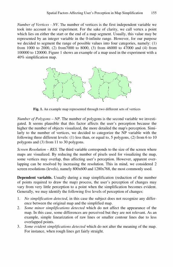
Number of Vertices - NV. The number of vertices is the first independent variable we took into account in our experiment. For the sake of clarity, we call vertex a point which lies on either the start or the end of a map segment. Usually, this value may be represented by an integer variable in the 0-infinite range. However, for our purpose we decided to segment the range of possible values into four categories, namely: (1) from 1000 to 2000, (2) from7000 to 8000, (3) from 46000 to 47000 and (4) from 100000 to 120000. Figure 1 shows an example of a map used in the experiment with a 40% simplification map.

Fig. 1. An example map represented through two different sets of vertices

Number of Polygons – NP. The number of polygons is the second variable we investi-gated. It seems plausible that this factor affects the user’s perception because the higher the number of objects visualized, the more detailed the map's perception. Simi-larly to the number of vertices, we decided to categorize the NP variable with the following three different levels: (1) less than, or equal to, 5 polygons, (2) from 6 to 10 polygons and (3) from 11 to 30 polygons.

Screen Resolution – RES. The third variable corresponds to the size of the screen where maps are visualized. By reducing the number of pixels used for visualizing the map, some vertices may overlap, thus affecting user’s perception. However, apparent over-lapping can be resolved by increasing the resolution. This in mind, we considered 2 screen resolutions (levels), namely 800x600 and 1280x768, the most commonly used.

Dependent variable. Usually during a map simplification (reduction of the number of points required to draw the map) process, the user’s perception of changes may vary from very little perception to a point when the simplification becomes evident. Generally, we may identify the following five levels of perception of changes:

1. No simplification detected, in this case the subject does not recognize any differ-ence between the original map and the simplified map.

2. Some minor simplifications detected which do not affect the appearance of the map. In this case, some differences are perceived but they are not relevant. As an example, simple linearization of raw lines or smaller contour lines due to less overlapped points.

3. Some evident simplifications detected which do not alter the meaning of the map. For instance, when rough lines get fairly straight.


4. Some substantial simplifications detected which affect the information the map conveys. The map is still recognizable but some changes may hide relevant de-tails. As examples, some peninsulas may disappear; boundaries may deeply alter their position, and so on.

5. The map can no longer be recognized.

Based on the above classification, we defined the Significant Simplification Rate (SSR) as the simplification rate which makes the user’s perception move from level 2 to level 3.

Participants. The participants we used in this research were students following the degree programme of Computer Science at the faculty of Science, University of Salerno (Italy). The complete list of individuals involved 144 subjects divided into 24 groups, namely 6 subjects per group. In order to make such groups as independent as possible we decided to randomly assign subjects to groups.

The rationale behind the choice of 24 groups is that 24 is exactly the number of different combinations of values for NP, NV and RES. All subjects were asked to complete a background information sheet in order to collect both personal data and data about their experiences with computer technology and, possibly, with GIS, also in terms of the exams they had already passed and the marks they had obtained.

We were interested in understanding how people who generally have marginal ex-perience with maps perceive different levels of simplification. Consequently, we avoided subjects who work with maps or had attended some GIS courses. Actually, the individuals we selected knew the most popular map applications, such as some web-based path finders, Google Map, etc. As for their age, they ranged between 20 and 30 years old.

Apparatus. As for the apparatus, we exploited three software applications, namely, SYSTAT™ [20], MapShaper [1] and ESRI ArcView™ [6]. They were run on a Windows XP© Professional platform mounted on a computer based on a Pentium Centrino™ processor with 1G RAM, a 72 Gb HD at 7200 rpm and a 15.4’’ multi resolution display. We used MapShaper for producing the reduced maps. It is a free online editor for Poly-gon and Polyline Shapefiles. It has a Flash interface that runs in an ordinary web browser. Mapshaper supports the Douglas-Peucker (RDP) line simplification algorithm. Finally, we used the ESRI ArcView 3.2 to produce the source maps we used in the experiment and to express them also in terms of the combination of the factor levels for, respectively, the number of polygons (NP) the number of vertices (NV) and the screen resolution (SR).

Task. Every group was associated with a map which satisfies one of the 24 combina-tions of the independent variable levels. This map and a simplified version of it were successively shown to each subject in the group, for ten second intervals. Then, ac-cording to the scale concerning the perception of changes, we asked the subjects for a value between 1 and 5. This step was repeated, increasing the simplification rate, until either subjects reached the maximum simplification rate or rated 5 their perception of changes. For each subject we reported the value of SSR, namely the simplification rate registered when they detected some evident simplifications, which did not alter the meaning of the map (i.e., level 3 of perception).


Test. Once results have been collected we applied a three way ANOVA (Analysis of Variance). The theory and methodology of ANOVA was mainly developed by Fisher during the 1920s [18]. ANOVA is essentially a method for analyzing one, two, or more quantitative or qualitative variables on one quantitative response. ANOVA is useful in a range of disciplines when it is suspected that one or more factors might affect a response. ANOVA is essentially a method of analyzing the variance of a response, dividing it into the various components corresponding to the sources of variation, which can be identified. We are interested in studying two effects - the main effect determined by each factor separately and the possible interactions among the factors. The main effect is defined to be the change of the evaluated factor (the dependent variable) while changing the level of one of the independent variables. In some experiments, we may find that the difference in the response between the levels of one factor is not the same at all levels of the other factors. When this happens, some interaction occurs between these factors. Moreover, the ANOVA method allows us to determine whether a change in the responses is due to a change in a factor or due to a wrong sample selection.

Research Hypotheses. Before starting the operative phase, we formally claim the null hypotheses we wished to reject in our experiment.

Table 1. Experiment hypothesis

H1. There is no difference in the SSR means of the different levels of factor NV H2. There is no difference in the SSR means of the different levels of factor NP H3. There is no difference in the SRR means of the different levels of factor RES H4. There is no interaction between NP and NV on SSR. H5. There is no interaction between NV and RES on SSR. H6. There is no interaction between RES and NP on SSR. H7. The two-way NV*NP interaction is the same at every level of RES

As listed in Table 1, the first three hypotheses are concerned with the influence that each factor may have on the SSR measure, separately. The next three hypotheses are concerned with the pair-wise interaction between independent factors and its influ-ence on SSR. Finally the last hypothesis involves the study of the interaction among all three independent variables and its influence on SSR.

Assumptions. The ANOVA test is based on the following assumptions about the input data: (1) All observations are mutually independent; (2) All sample populations are normally distributed; (3) All sample populations have equal variance. The first assumption should be true on the basis of how we choose individuals and how we assigned them to groups.

The Shapiro-Wilk’s test (W) [18] is used in testing for normality. It is the preferred test of normality because of its good properties as compared to a wide range of alter-native tests. It is a standard test for normality used when the sample size is between 3 and 5000. The W-value given by this test is an indication of how good the fit is to a


normal variable, namely the closer the W-value is to 1, the better the fit is. In our case, high values of W are common to all the groups we took into account; therefore we should accept the hypothesis of normality for each group. Table 2 shows the W values obtained after having applied the Shapiro-Wilk Test to each group.

Table 2. Results of the Shapiro-Wilk Test

NP NV W (800x600) W (1024x768)<5 1k-2k 0.7 1.06-10 1k-2k 0.7 0.811-30 1k-2k 1.0 0.7<5 7k-8k 0.9 0.86-10 7k-8k 0.9 0.811-30 7k-8k 1.0 0.9<5 46k-47k 0.8 0.96-10 46k-47k 0.7 0.811-30 46k-47k 1.0 0.8<5 110k-120k 0.8 1.06-10 110k-120k 0.9 1.011-30 110k-120k 0.5 0.9

Next, we see the Levene's Test [18] for equality of variances. This tells us whether we have met our third assumption, namely whether the groups have approximately equal variance with respect to the SSR.

If the Levene's Test is significant (the value under p is less than 0.05), the variances are significantly different. If it is not significant (p is greater than 0.05), the variances are not significantly different; that is, the variances are approximately equal. In our case, we see that the significance is 0.6, which is greater than 0.05. Thus, we can assume that the variances are approximately the same.

Since the controls we made confirm our expectations, we may claim that assump-tions have been respected and that data and groups are proper for the analysis we want to perform.

Results. The ANOVA Table 31 shows, for each factor, the number of degree of free-dom (DF), the sum of squares (SS), the mean of the squares (Mean Square), the value of the statistical (F-Ratio), its significance level (Sig. Level) and the F critical value; if the Sig. Level is smaller than 0.05, then the factor effect is statistically significant at the level of confidence of 95%. The significant factors and their significance levels are highlighted in boldface in the tables. This kind of tabular representation is cus-tomarily used to set out the results of ANOVA calculations.

1 In this test we firstly fixed the acceptable error (5%) which together with the Df implies the F-

critical. If the calculated F-ratio is greater than the F-critical means that the test is significative and the null hypothesis should be rejected. The p-value specifies the probability that the F-ratio is greater of the F-critical. Generally, a p-value smaller than 0.05 tell us that this prob-ability is greater than 95%. Type III SS and Mean Squares are intermediate values required to calculate the F-Ratio.


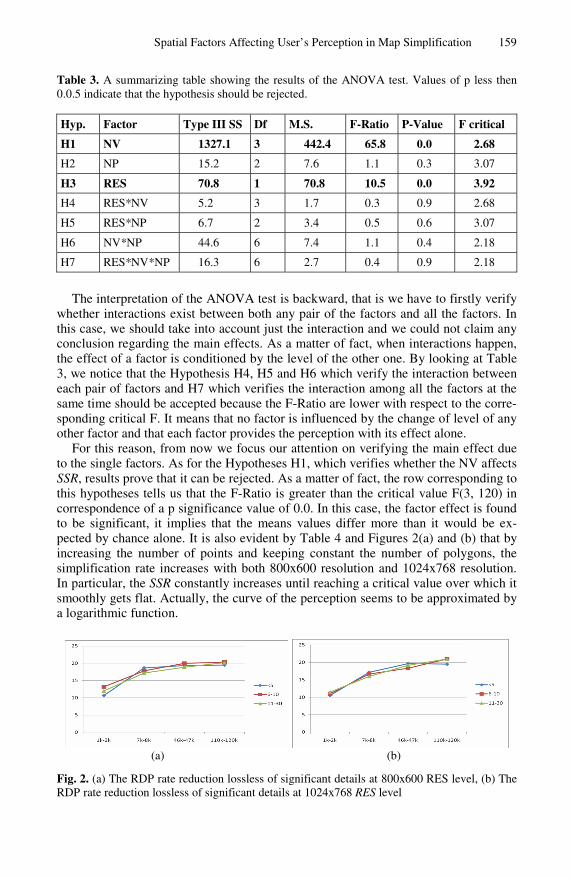
Table 3. A summarizing table showing the results of the ANOVA test. Values of p less then 0.0.5 indicate that the hypothesis should be rejected.

Hyp. Factor Type III SS Df M.S. F-Ratio P-Value F critical

H1 NV 1327.1 3 442.4 65.8 0.0 2.68

H2 NP 15.2 2 7.6 1.1 0.3 3.07

H3 RES 70.8 1 70.8 10.5 0.0 3.92

H4 RES*NV 5.2 3 1.7 0.3 0.9 2.68

H5 RES*NP 6.7 2 3.4 0.5 0.6 3.07

H6 NV*NP 44.6 6 7.4 1.1 0.4 2.18

H7 RES*NV*NP 16.3 6 2.7 0.4 0.9 2.18

The interpretation of the ANOVA test is backward, that is we have to firstly verify whether interactions exist between both any pair of the factors and all the factors. In this case, we should take into account just the interaction and we could not claim any conclusion regarding the main effects. As a matter of fact, when interactions happen, the effect of a factor is conditioned by the level of the other one. By looking at Table 3, we notice that the Hypothesis H4, H5 and H6 which verify the interaction between each pair of factors and H7 which verifies the interaction among all the factors at the same time should be accepted because the F-Ratio are lower with respect to the corre-sponding critical F. It means that no factor is influenced by the change of level of any other factor and that each factor provides the perception with its effect alone.

For this reason, from now we focus our attention on verifying the main effect due to the single factors. As for the Hypotheses H1, which verifies whether the NV affects SSR, results prove that it can be rejected. As a matter of fact, the row corresponding to this hypotheses tells us that the F-Ratio is greater than the critical value F(3, 120) in correspondence of a p significance value of 0.0. In this case, the factor effect is found to be significant, it implies that the means values differ more than it would be ex-pected by chance alone. It is also evident by Table 4 and Figures 2(a) and (b) that by increasing the number of points and keeping constant the number of polygons, the simplification rate increases with both 800x600 resolution and 1024x768 resolution. In particular, the SSR constantly increases until reaching a critical value over which it smoothly gets flat. Actually, the curve of the perception seems to be approximated by a logarithmic function.

(a) (b)

Fig. 2. (a) The RDP rate reduction lossless of significant details at 800x600 RES level, (b) The RDP rate reduction lossless of significant details at 1024x768 RES level


Table 4. Statistical about NV factor

Factor Level LSM SErr N

NV 1K-2K 11.5 0.4 36

NV 7K-8K 17.2 0.4 36

NV 46K-47K 18.7 0.4 36

NV 110K-120K 19.0 0.4 36

• 1K and 2K may be approximately reduced around at 65% (11.5 RDP rate) with-out loss of significant details,

• 7K and 8K may be simplified around at 72% (17.2 RDP rate), • 46K and 47K may be simplified around at 72% (18.7 RDP rate) and • 110K and 120K may be simplified around at 76% (19.0 RDP rate).

By taking into account such values and their meanings we can observe that any map we are managing, which has more than 1K vertices, may be approximated by a reduced one having less than 65% of the original vertices. As an example, a map having 1000 vertices may be reduced through the RDP algorithm to a map having 350 vertices without loss of significant details. As the number of vertices increases this percentage slightly augments as shown in the previous figures. As for Hypotheses H2, results are summarized in Table 3 and 4, Figures 3(a) and (b).

Table 5. Statistical about the Number of Polygons factor


NP A < 5 16.6 0.4 48

NP B 6-10 17.0 0.4 48

NP C 11-30 16.2 0.4 48

Table 1 highlights that we cannot reject this hypothesis and this factor does not af-fect the perception of the subjects. This claim is fundamentally proved by two obser-vations. The first one is that the least squares means (LSM) obtained by varying the number of polygons and keeping constant the number of vertices are substantially similar (16.6, 17, 16.2). The second one is that the ANOVA test calculates an F-Ratio (1.1) is smaller than the corresponding F-critical (F(2,120)=3.07).

Graphically, Figures 3(a) (800x600) and 11 (1024x768) show that for each level of the NV variable (4) the SSR diagrams are essentially straight lines, which confirms the numerical results, namely for each level there is a substantial flattening of the means.

Thus, we can deduce that the NP factor does not affect the significant simplifica-tion rate. As a matter of fact, this assertion might be interpreted as the fact that the perception of significant changes is not affected by the inner complexity of the map or, we can claim that any set of maps having a similar number of points but with dif-ferent number of polygons may be reduced using the same RDP rate obtaining no significant differences with respect to the original ones. From a practical point of view, as an example, it means that two maps of 100k vertices, the first one composed


(a) (b)

Fig. 3. (a)The diagram of the least square means considering NV constant and changing NP at 800x600 RES level, (b) The diagram of the least square means considering NV constant and changing NP at 1024x768 RES level

Fig. 4. The diagram of the least square means considering constant NV and NP and changing the RES levels

of one polygon while the second one composed by 100 polygons may be reduced using just the 30% of the original points without loosing significant details.

The last main factor we examine is RES (Hypotheses H3). Table 3 shows that the corresponding F-Ratio is greater than the critical F associated with the relative degree of freedom (F(1, 120)=3.92). Similarly to NV, it means we have to reject the null hypotheses, namely that in this case the variability is especially due to the effect of the RES factor. This claim may be considered highly significant because the p value is close to 0. As a matter of fact, The RES factor is relevant with respect to the simplifi-cation rate. Table 6 shows that RES decreases on the average from 17.3 to 15.9 pass-ing from the 800x600 to 1024x768 resolution. It means that by increasing the screen resolution, subjects are more able to perceive significant differences between the original map and the reduced one. It is further proved by Figure 4. As a matter of fact, most of lines pass from a higher value to a lower one.

Table 6. Statistical about the RES factor


RES 800x600 17.3 0.3 72

RES 1280x768 15.9 0.3 72


4 Conclusion and Future Work

In this paper, we have carried out an empirical study aimed at finding out which fac-tors affect the user’s perception of significant changes (SSR) after simplification us-ing the Ramer-Douglas-Peucker algorithm. We have considered three factors, NP, NV and RES. We have proved that there does not exist significant interactions among any pair or triple of the above factors. Successively, we measured the contribution each factor provides to perception and we found out that just NV and RES give significant effects while NP does not. As for RES, the SSR decreases on the average from 17.3 to 15.9 passing from the 800x600 to 1024x768 resolution. It means that by increasing the screen resolution, subjects perceive earlier significant differences between the original map and the reduced one. Finally, as for NP, we proved that there are no significant differences by changing the levels in terms of SSR. As a matter of fact, it means that the complexity of the map in terms of number of contained objects is not relevant to the aim of map reduction.

In the future, we think to verify whether other kinds of factors affect the SSR. As an example, we want to perform experiments considering also the roughness degree, the size of the presented map and some other RES levels. Successively, we want to apply the results we found out to some of the application fields we showed at the begin of the paper. As an example, we want to build up a new layer which is inter-posed between users and map servers in order to speed up the transmission of maps automatically reducing the number of vertexes effectively transmitted over the net-work. We want also implement progressive map transmission based on the data we gathered and we do not employed in this experiment.

References

1. Bloch, M., Harrower, M.: MapShaper.org: A Map Generalization Web Service. In: Proc. of Autocarto 2006, Vancouver, Canada, June 26-28 (2006)

2. Buttenfield, B., McMaster, R.B.: Map Generalization: Making Rules for knowledge repre-sentation, Longman Group, UK (1991)

3. Cromley, R.G., Campbell, G.M.: Integrating quantitative and qualitative aspects of digital line simplification. The Cartographic Journal 29(1), 25–30 (1992)

4. Douglas, D., Peucker, T.: Algorithms for the reduction of the number of points required to represent a digitized line or its caricature. The Canadian Cartographer 10(2) (1973)

5. Dutton, G.: Scale, Sinuosity, and Point Selection in Digital Line Generalization. Cartogra-phy and Geographic Information Science 26(1), 33–53 (1999)

6. ESRI ArcView, http://www.esri.com (accessed 3.2. 03/06/08) 7. Hershberger, J., Snoeyink, J.: Speeding up the Douglas-Peucker line simplification algo-

rithm. In: Proc. 5th Intl. Symp. on Spatial Data Handling, vol. 1, pp. 134–143 (1992) 8. Kazemi, S., Lim, S.: Deriving Multi-Scale GEODATA from TOPO-250K Road Network

Data. Journal of Spatial Science 52(1) (2007) 9. Kazemi, S., Lim, S., Rizos, C.: A review of Map and Spatial Database Generalization for

Developing a Generalization Framework. In: ISPRS Conference, Generalization and Data Mining (2004)

10. Lee, D.: Generalization within a geoprocessing framework. In: Proceedings of GEOPRO 2003 Workshop, Mexico City, November, pp. 1–10 (2003)


11. MacEachren, A.M.: How maps work: Representation, visualization, and design. Guilford Press, New York (1995)

12. McMaster, R.B., Shea, K.S.: Generalization in Digital Cartography. Association of Ameri-can Geographer, Washington (1992)

13. Montello, D.R.: Cognitive map design research in the twentieth century: Theoretical and empirical approaches. Cartography and Geographic Information Science 29(3) (2002)

14. Montello, D.R., Golledge, R.: Scale and Detail in the Cognition of Geographic Informa-tion. University of California, California (1999),

http://www.ncgia.ucsb.edu/Publications/Varenius_Reports/ Scale_and_Detail_in_Cognition.pdf

15. Nakos, B.: Comparison of manual versus digital line generalization. In: Proceedings of Workshop on Generalization, Ottawa, Canada (August 1999)

16. Ramer, U.: An iterative procedure for the polygonal approximation of plane curves. Com-puter Graphics and Image Processing 1, 244–256 (1972)

17. Saalfeld, A.: Topologicaljy Consistent Line Simplification with the RDP Algorithm. Car-tography and Geographic Information Science 26(1), 7–18 (1999)

18. Sheldon, M.R.: Introduction to probability and Statistics for Engineers and Scientists, 2nd edn. Academic Press, London (2003)

19. Slocum, T.A., Blok, C., Jiang, B., Koussoulakou, A., Montello, D.R., Fuhrmann, S., Hed-ley, N.R.: Cognitive and usability issues in geovisualization. Cartography and Geographic Information Science 28, 61–75 (2001)

20. SYSTAT ver.12., http://www.systat.com 21. Topfer, F., Pilliwizer, W.: The Principles of Map Selection. The Cartographic Journal 3,

10–16 (1966) 22. Visvalingam, M., Whyatt, J.D.: Line generalization by repeated elimination of points. The

Cartographic Journal 30(1), 46–51 (1993) 23. Visvalingam, M., Williamson, P.J.: Simplification and generalization of large-scale data

for roads - a comparison of two filtering algorithms. Cartography and Geographic Informa-tion Systems 22(4), 264–275 (1995)

24. Wang, Z., Muller, J.C.: Line generalization based on analysis of shape characteristics. Car-tography and Geographic Information Systems 25(1), 3–15 (1998)

25. Wu, S.T., Márquez, M.R.G.: A non-self-intersection Douglas-Peucker Algorithm. In: Pro-ceedings Brazilian Symposium on Computer Graphics and Image Processing, SIB-GRAPHI XVI (2003)

26. Zhao, H., Li, X., Jiang, L.: A modified Douglas-Peucker simplification algorithm. In: Proc. of Geoscience and Remote Sensing Symposium (IGARSS 2001), Sydney, Australia (2001)

Spatial Factors Affecting User's Perception in Map Simplification: An Empirical Analysis

Documents

Transcript of Spatial Factors Affecting User's Perception in Map Simplification: An Empirical Analysis