
Sparse Representation of Visual Data for Compression and ...
179
Linköping studies in science and technology. Dissertation, No. 1963 SPARSE REPRESENTATION OF VISUAL DATA FOR COMPRESSION AND COMPRESSED SENSING Ehsan Miandji Division of Media and Information Technology Department of Science and Technology Linköping University, SE-601 74 Norrköping, Sweden Norrköping, December 2018
-
Upload
khangminh22 -
Category
Documents
-
view
2 -
download
0
Transcript of Sparse Representation of Visual Data for Compression and ...
Linköping studies in science and technology.Dissertation, No. 1963
SPARSE REPRESENTATION OF VISUAL DATA FORCOMPRESSION AND COMPRESSED SENSING
Ehsan Miandji
Division of Media and Information TechnologyDepartment of Science and Technology
Linköping University, SE-601 74 Norrköping, SwedenNorrköping, December 2018

Description of the cover image
The cover of this thesis depicts the sparse representation of a lightfield. From the back side to front, a light field is divided intosmall elements, then these elements (signals) are projected onto anensemble of two 5D dictionaries to produce a sparse coefficient vector.I hope that the reader can deduce where the dimensionality of thoseRubik’s Cube looking matrices come from after reading Chapter3 of this thesis. The light field used on the cover is a part of theStanford Lego Gantry database (http://lightfield.stanford.edu/)
Sparse Representation of Visual Data for Compression andCompressed Sensing
Copyright © 2018 Ehsan Miandji (unless otherwise noted)
Division of Media and Information TechnologyDepartment of Science and Technology
Linköping University, Campus NorrköpingSE-601 74 Norrköping, Sweden
ISBN: 978-91-7685-186-9 ISSN: 0345-7524Printed in Sweden by LiU-Tryck, Linköping, 2018


Abstract
The ongoing advances in computational photography have introduced a rangeof new imaging techniques for capturing multidimensional visual data such aslight fields, BRDFs, BTFs, and more. A key challenge inherent to such imagingtechniques is the large amount of high dimensional visual data that is produced,often requiring GBs, or even TBs, of storage. Moreover, the utilization of thesedatasets in real time applications poses many difficulties due to the large memoryfootprint. Furthermore, the acquisition of large-scale visual data is very challengingand expensive in most cases. This thesis makes several contributions with regardsto acquisition, compression, and real time rendering of high dimensional visualdata in computer graphics and imaging applications.
Contributions of this thesis reside on the strong foundation of sparse represen-tations. Numerous applications are presented that utilize sparse representationsfor compression and compressed sensing of visual data. Specifically, we present asingle sensor light field camera design, a compressive rendering method, a real timeprecomputed photorealistic rendering technique, light field (video) compressionand real time rendering, compressive BRDF capture, and more. Another keycontribution of this thesis is a general framework for compression and compressedsensing of visual data, regardless of the dimensionality. As a result, any type ofdiscrete visual data with arbitrary dimensionality can be captured, compressed,and rendered in real time.
This thesis makes two theoretical contributions. In particular, uniqueness conditionsfor recovering a sparse signal under an ensemble of multidimensional dictionaries ispresented. The theoretical results discussed here are useful for designing efficientcapturing devices for multidimensional visual data. Moreover, we derive theprobability of successful recovery of a noisy sparse signal using OMP, one of themost widely used algorithms for solving compressed sensing problems.
v


PopulärvetenskapligSammanfattning
Den snabba ökningen i beräkningskapacitet hos dagens datorer har de senaste årenbanat väg för utveckling av en rad kraftfulla verktyg och metoder inom bildteknik,s.k. “computational photography”, inom vilka bildsensorer och optiska uppställning-ar kombineras med beräkningar för att skapa nya bildtillämpningar. Den visuelladata som beräknas fram är oftast av högre dimensionalitet än vanliga bilder i 2D,dvs. resultatet är inte en bild som består av ett plan av bildpunkter i 2D utan endatamängd i 3D, 4D, 5D, . . . , nD. Det grundläggande målet med dessa metoder äratt ge användaren helt nya verktyg för att analysera och uppleva data med nyatyper av interaktion- och visualiseringstekniker. Inom datorgrafik och datorseende,som är de drivande forskningsområdena, har det t.ex. introducerats tillämpningarsåsom 3D-video (stereo), ljusfält (dvs. bilder och video där användaren i efterhandi 3D interaktivt kan ändra betraktningsvinkel, fokus eller zoom-nivå), displayersom tillåter 3D utan 3D-glasögon, metoder för mycket högupplöst skanning avmiljöer och objekt, och metoder för mätning av materials optiska egenskaper förfoto-realistisk visualisering av t.ex. produkter. Inom områden såsom radiologi ochsäkerhet hittar vi också bildtillämpningar, t.ex. röntgen, datortomografi eller mag-netresonanskamera där beräkningar och sensorer kombineras för att skapa datasom kan visualiseras i 3D, eller 4D om mätningen är utförd över tid. Ett centraltproblem hos alla dessa tekniker är att de genererar mycket stora datamängder, oftai storleksordningen hundratals GB eller till och med flera TB. En viktig forsknings-fråga är därför att utveckla ny teori och praktiska metoder för effektiv kompressionoch lagring av högdimensionell visuell data. En lika viktig aspekt är att utveck-la representationer och algoritmer som utöver effektiv lagring tillåter interaktivdatabehandling, visualisering och uppspelning av data, t.ex. ljusfältsvideo.
Den här avhandlingen introducerar en rad nya representationer för inspelning,databehandling och lagring av högdimensionell visuell data. Den omfattar tvåhuvudområden: effektiva representationer för kompression, databehandling ochvisualisering, samt effektiv mätning av högdimensionella visuella signaler baseratpå s.k. compressive sensing. Avhandlingen och de ingående artiklarna introduceraren rad bidrag i form av teori, algoritmer och metoder inom båda dessa områden.
Det första huvudområdet i avhandlingen fokuserar på utveckling av en uppsättningdatarepresentationer som med hjälp av maskininlärnings- och optimeringsmeto-der anpassar sig till data. Detta möjliggör optimala representationer baserat påett antal kriterier, t.ex. att representationen ska vara så kompakt (komprimerad)som möjligt och att de approximationsfel som introduceras vid rekonstruktion
vii
viii
av signalen är så små som möjligt. Dessa representationer bygger på s.k. glesa(på engelska “sparse”) basfunktioner. En uppsättning basfunktioner kallas för enordbok (“dictionary”) och en signal, t.ex. en bild, video eller ett ljusfält, represen-teras som en kombination av basfunktioner från ordboken. Om representationentillåter att signalen kan beskrivas med ett litet antal basfunktioner, motsvarandeen mindre informationsmängd än originalsignalen, leder detta till att signalenkomprimeras. I den teori och de tekniker som har utvecklats inom ramarna förden här avhandlingen optimeras basfunktionerna och ordboken utifrån den typav data som ska representeras. Detta gör det möjligt att beskriva en signal medett mycket litet antal basfunktioner, vilket leder till mycket effektiv komprimeringoch lagring. De utvecklade representationerna är specifikt designade så att allacentrala beräkningar kan ske parallellt per datapunkt. Genom att utnyttja kraftenhos moderna GPUer är det därför möjligt att i realtid hantera och visualiseramycket minneskrävande visuella signaler.
Det andra området i avhandlingen tar sin startpunkt i att de representationer ochbasfunktioner som har utvecklats för kompression gör det möjligt att på ett mycketeffektivt sätt applicera moderna mät- och samplingsmetoder, compressive sensing,på bilder, video, ljusfält och andra visuella signaler. Den teori compressive sensingbygger på visar att en signal kan mätas och rekonstrueras från ett mycket lågtantal mätpunkter om mätningen utförs i en bas, representation, där signalen sommäts är gles/sparse. Genom att utnyttja denna egenskap utvecklar avhandlingenteori för hur compressive sensing kan användas för mätning och rekonstruktionav visuella signaler oavsett dess dimensionalitet samt demonstrerar genom en radolika exempel hur compressive sensing kan appliceras i praktiken.

Acknowledgments
I have been fortunate enough to work and collaborate with the most amazing andknowledgeable people I have ever met through my years as a PhD student. Therefore,I found writing this section of my thesis to be the most difficult one because puttinginto words my sincere gratitudes towards my supervisor, co-supervisor, colleagues,friends, and family is NP-hard. But I will try.
First and foremost, I would like to thank my supervisor, Jonas Unger, for hisguidance, support, and patience throughout my years as a PhD student. Yourenthusiasm for research always encouraged me to do more and more. What ajourney this was! Hectic at times, but never ceasing to be fun. I cannot imaginebeing the academically grown person I am today without your guidance. And I willbe forever grateful for the balance you provided between the supervision and thefreedom to do research independently. If it wasn’t for the academic freedom youprovided, I wouldn’t have discovered my favorite research topics. And if it wasn’tfor your guidance, I wouldn’t have progressed as much in those topics. It has beena privilege working with you and I hope that our collaborations will continue. Iwould like to thank my co-supervisor, Anders Ynnerman. You have established aresearch environment with the highest standards and I thank you for giving methe chance to be a PhD student at the MIT division.
I would like to thank my colleagues at the computer graphics and image processinggroup. I am very grateful for being among you during my PhD studies. First, PerLarsson, the man behind all the cool research gadgets I used during my studies.Funny, kind, and intelligent, you have it all Per! Gabriel Eilertsen, the HDR guruin our group with the most amazing puns. Thank you Saghi Hajisharif, you simplyare the best (my totally unbiased opinion). I am very grateful for all the goodcollaborations we had. Thank you Tanaboon Tongbuasirilai for helping me with theBRDF renderings included in this thesis and all the enjoyable discussions we had.Thank you Apostolia Tsirikoglou, our deep learning expert, for lighting up the officewith your jokes. And thanks to the previous members of the group with whom Ispent the majority of my PhD studies. Specifically, thank you Joel Kronander forall the memorable discussions we had as PhD students from compressed sensing torendering and beyond! Thank you for the collaborations we had; it was a privilegeand I truly miss you in the lab. And by the way, “spike ensemble” is the new“sub-identity”. Thank you Andrew Gardner, also known as the coding guru, forour collaborations on the compression library. We miss you! And last but notleast, thank you Eva Skärblom for arranging everything from the travel plans tomy salary!
Thank you Mohammad Emadi for two years of long distance collaboration on our
ix

x
work towards Paper F and Paper G. You are a brilliant mind! I also would like tothank Christine Guillemot, the head of SIROCCO team at INRIA, Rennes, France,who gave me the opportunity for a research visit. I truly enjoyed my time thereand I am grateful for our collaboration that led to Paper E.
Thank you Saghi for making my life what I always wanted it to be. I cannotimagine going through the difficult times without the hope and happiness youbrought. And thank you for your understanding during the stressful time of writingthis thesis. I am incomplete without you, to the extent that even compressedsensing cannot recover me.
Ali Samini, my dear boora, I am so happy that I came to Sweden because otherwiseI most probably wouldn’t have met you. I had some of the best times in my lifeduring our years as PhD students and you have always been there in my difficulttimes. Thank you Alexander Bock, my German brother, for all the good timeswe had together during my PhD studies. Thanks to my dearest friends in Iran:Aryan, Javid, Kamran (the 3 + 1 musketeers). Every time I went back to Iran andvisited you guys, all the tiredness gathered during the year from the deadlines justvanished.
And last but certainly not least, I would like to thank my parents, Shamsi andDavood. Thank you for placing such a high value on education since my childhood.You have always pushed me to achieve more on every step of my life. I am eternallygrateful for everything you have done for me.
List of Publications
The published work of the author that are included in this thesis is listed below inreverse chronological order.
• E. Miandji, S. Hajisharif, and J. Unger, “A Unified Framework for Compressionand Compressed Sensing of Light Fields and Light Field Videos,” ACMTransactions on Graphics, Provisionally accepted
• E. Miandji, J. Unger, and C. Guillemot, “Multi-Shot Single Sensor Light FieldCamera Using a Color Coded Mask,” in 26th European Signal ProcessingConference (EUSIPCO) 2018. IEEE, Sept 2018
• E. Miandji†, M. Emadi†, and J. Unger, “OMP-based DOA Estimation Perfor-mance Analysis,” Digital Signal Processing, vol. 79, pp. 57–65, Aug 2018,† equal contributor
• E. Miandji†, M. Emadi†, J. Unger, and E. Afshari, “On Probability of Sup-port Recovery for Orthogonal Matching Pursuit Using Mutual Coherence,”IEEE Signal Processing Letters, vol. 24, no. 11, pp. 1646–1650, Nov 2017,† equal contributor
• E. Miandji and J. Unger, “On Nonlocal Image Completion Using an Ensemble ofDictionaries,” in 2016 IEEE International Conference on Image Processing(ICIP). IEEE, Sept 2016, pp. 2519–2523
• E. Miandji, J. Kronander, and J. Unger, “Compressive Image Reconstruction inReduced Union of Subspaces,” Computer Graphics Forum, vol. 34, no. 2, pp.33–44, May 2015
• E. Miandji, J. Kronander, and J. Unger, “Learning Based Compression of SurfaceLight Fields for Real-time Rendering of Global Illumination Scenes,” inSIGGRAPH Asia 2013 Technical Briefs. ACM, 2013, pp. 24:1–24:4
Other publications by the author that are relevant to this thesis but were notincluded are:
• G. Baravdish, E. Miandji, and J. Unger, “GPU Accelerated Sparse Representationof Light Fields,” in 14th International Conference on Computer Vision Theoryand Applications (VISAPP 2019), submitted
xi
xii
• E. Miandji†, M. Emadi†, and J. Unger, “A Performance Guarantee for OrthogonalMatching Pursuit Using Mutual Coherence,” Circuits, Systems, and SignalProcessing, vol. 37, no. 4, pp. 1562–1574, Apr 2018, † equal contributor
• J. Kronander, F. Banterle, A. Gardner, E. Miandji, and J. Unger, “PhotorealisticRendering of Mixed Reality Scenes,” Computer Graphics Forum, vol. 34,no. 2, pp. 643–665, May 2015
• S. Mohseni, N. Zarei, E. Miandji, and G. Ardeshir, “Facial Expression RecognitionUsing Facial Graph,” in Workshop on Face and Facial Expression Recogni-tion from Real World Videos (ICPR 2014). Cham: Springer InternationalPublishing, 2014, pp. 58–66
• S. Hajisharif, J. Kronander, E. Miandji, and J. Unger, “Real-time Image BasedLighting with Streaming HDR-light Probe Sequences,” in SIGRAD 2012:Interactive Visual Analysis of Data. Linköping University Electronic Press,Nov 2012
• E. Miandji, J. Kronander, and J. Unger, “Geometry Independent Surface LightFields for Real Time Rendering of Precomputed Global Illumination,” inSIGRAD 2011. Linköping University Electronic Press, 2011
• E. Miandji, M. H. Sargazi Moghadam, F. F. Samavati, and M. Emadi, “Real-time Multi-band Synthesis of Ocean Water With New Iterative Up-samplingTechnique,” The Visual Computer, vol. 25, no. 5, pp. 697–705, May 2009
Contributions
In what follows, the main publications included in this thesis are listed, where ashort description of each paper along with author’s contributions are presented.
Paper A: Learning Based Compression of Surface Light Fields for Real-time Rendering of Global Illumination Scenes
E. Miandji, J. Kronander, and J. Unger, “Learning Based Compressionof Surface Light Fields for Real-time Rendering of Global IlluminationScenes,” in SIGGRAPH Asia 2013 Technical Briefs. ACM, 2013, pp.24:1–24:4
This paper presents a method for real time photorealistic precomputed rendering ofstatic scenes with arbitrarily complex materials and light sources. To achieve this,a training-based method for compression of Surface Light Fields (SLF) using anensemble of orthogonal two-dimensional dictionaries is presented. We first generatean SLF for each object of a scene using the PBRT library [15]. Then, an ensembleis trained for each SLF in order to represent the SLF using sparse coefficients. Toaccelerate training and exploit the local similarities in each SLF, the authors useK-Means [16] for clustering prior to training an ensemble. Real time performanceis achieved by local reconstruction of the compressed set of SLFs using the GPU.The author of this thesis was responsible for the design and implementation of thealgorithm, as well as the majority of the written presentation.
Paper B: A Unified Framework for Compression and Compressed Sens-ing of Light Fields and Light Field Videos
E. Miandji, S. Hajisharif, and J. Unger, “A Unified Framework forCompression and Compressed Sensing of Light Fields and Light FieldVideos,” ACM Transactions on Graphics, Provisionally accepted
This work is an extension of Paper A with several contributions. We propose amethod for training n-dimensional (nD) dictionaries that enable enhanced sparsitycompared to 2D and 1D variants used in the previous work. The proposed methodadmits sparse representation and compressed sensing of arbitrarily high dimensionaldatasets, including light fields (5D), light field videos (6D), bidirectional texturefunctions (7D) and spatially varying BRDFs (7D). We also observed that K-Meansis not adequate for capturing self-similarities of complex high dimensional datasets.
xiii
xiv
Therefore, we present a pre-clustering method that is based on sparsity, ratherthan the `2 norm, while being resilient to noise and outliers. The ensemble ofmultidimensional dictionaries enables real-time rendering of large-scale light fieldvideos. The author of this thesis was responsible for the design of the framework,and contributed to the majority of the implementation and written presentation.
Paper C: Compressive Image Reconstruction in Reduced Union of Sub-spaces
E. Miandji, J. Kronander, and J. Unger, “Compressive Image Recon-struction in Reduced Union of Subspaces,” Computer Graphics Forum,vol. 34, no. 2, pp. 33–44, May 2015
This paper presents a novel compressed sensing framework using an ensemble oftrained 2D dictionaries. The framework was applied for compressed sensing ofimages, videos, and light fields. While the trained ensemble is 2D, the compressedsensing was applied to 1D patches using the construction of a Kronecker ensemble.Using point sampling as the sensing matrix, the framework is shown to be effectivefor accelerating photo realistic rendering, as well as light field imaging. The resultsshow significant improvements over state of the art methods in graphics and imageprocessing literature. The author was responsible for the design and implementationof the method, as well as the majority of its written presentation.
Paper D: On Nonlocal Image Completion Using an Ensemble of Dictio-naries
E. Miandji and J. Unger, “On Nonlocal Image Completion Using anEnsemble of Dictionaries,” in 2016 IEEE International Conference onImage Processing (ICIP). IEEE, Sept 2016, pp. 2519–2523
This paper presents a theoretical analysis on the compressed sensing frameworkintroduced in Paper C. In particular, we derive a lower bound on the number ofpoint samples and the probability of success for exact recovery of an image ora light field. The lower bound is dependent on the coherence of dictionaries inthe ensemble. The theoretical results presented are useful for designing efficientdictionary ensembles for light field imaging. In Paper B, we reformulate theseresults for nD dictionary ensembles. The author was responsible for the design,implementation, and the written presentation of the method. The paper waspresented by Jonas Unger at ICIP 2016, Phoenix, Arizona.
xv
Paper E: Multi-Shot Single Sensor Light Field Camera Using a ColorCoded Mask
E. Miandji, J. Unger, and C. Guillemot, “Multi-Shot Single SensorLight Field Camera Using a Color Coded Mask,” in 26th EuropeanSignal Processing Conference (EUSIPCO) 2018. IEEE, Sept 2018
In this paper, a compressive light field imaging system based on the coded aperturedesign is presented. A color coded mask is placed between the aperture and thesensor. It is shown that the color coded mask is significantly more effective thanthe previously used monochrome masks [17]. Moreover, by micro movementsof the mask and capturing multiple shots, one can incrementally improve thereconstruction quality. In addition, spatial sub-sampling is proposed to provide atrade off between the quality and speed of reconstruction. The proposed methodachieves up to 4dB in PSNR over [17]. The majority of this work was done whenthe author was working as a visiting researcher at SIROCCO lab, a leading lightfield research group at INRIA, Rennes, France, led by Christine Guillemot. Theauthor was responsible for the design and implementation of the method, andcontributed to the majority of the written presentation.
Paper F: On Probability of Support Recovery for Orthogonal MatchingPursuit Using Mutual Coherence
E. Miandji†, M. Emadi†, J. Unger, and E. Afshari, “On Probabilityof Support Recovery for Orthogonal Matching Pursuit Using MutualCoherence,” IEEE Signal Processing Letters, vol. 24, no. 11, pp. 1646–1650, Nov 2017, † equal contributor
This paper presents a novel theoretical analysis of the Orthogonal Matching Pursuit(OMP), one of the most commonly used greedy sparse recovery algorithm forcompressed sensing. We derive a lower bound for the probability of identifyingthe support of a sparse signal contaminated with additive Gaussian noise. Mutualcoherence is used as a metric for the quality of a dictionary and we do not assumeany structure for the dictionary, or the sensing matrix; hence, the theoretical resultscan be utilized in any compressed sensing framework, e.g. Paper B, Paper C, andPaper E. The new bound significantly outperforms the state of the art [18]. Theauthor of this thesis and Mohammad Emadi equally contributed to this work. Theproject was carried out in collaboration with the Cornell University (and later onthe University of Michigan).
xvi
Paper G: OMP-based DOA estimation performance analysis
E. Miandji†, M. Emadi†, and J. Unger, “OMP-based DOA EstimationPerformance Analysis,” Digital Signal Processing, vol. 79, pp. 57–65,Aug 2018, † equal contributor
Presents an extension of the theoretical work in Paper F. We derive an upper boundfor the Mean Square Error (MSE) of OMP given a dictionary, the signal sparsity,and the signal’s noise properties. Using this upper bound, we derive new lowerbounds for the probability of support recovery. Compared to Paper F, the newbounds are formulated using more "user-friendly" parameters such as the signal tonoise ratio and the dynamic range. Furthermore, these new bounds shed light onthe special properties of the bound derived in Paper F. In addition, here we considerthe more general case of complex valued signals and dictionaries. Although theapplication considered in the paper is estimating the Direction of Arrival (DOA)for sensor arrays, the theoretical results presented are relevant to this thesis. Theauthor of this thesis and Mohammad Emadi equally contributed to this work.
Contents
Abstract v
Populärvetenskaplig Sammanfattning vii
Acknowledgments ix
List of Publications xi
Contributions xiii
1 Introduction 11.1 Sparse Representation 41.2 Compressed Sensing 91.3 Thesis outline 111.4 Aim and Scope 12
2 Preliminaries 152.1 Notations 152.2 Tensor Approximations 162.3 Sparse Signal Estimation 192.4 Dictionary Learning 222.5 Visual Data: The Curse/Blessing of Dimensionality 26
3 Learning-based Sparse Representation of Visual Data 293.1 Outline and Contributions 303.2 Multidimensional Dictionary Ensemble 30
3.2.1 Motivation 313.2.2 Training 343.2.3 Testing 37
3.3 Pre-clustering 393.3.1 Motivation 393.3.2 Aggregate Multidimensional Dictionary Ensemble 41
3.4 Summary and Future Work 43
4 Compression of Visual Data 454.1 Outline and Contributions 454.2 Precomputed Photorealistic Rendering 46
4.2.1 Background and Motivation 464.2.2 Overview 484.2.3 Data Generation 48
xvii
Contents
4.2.4 Compression 484.2.5 Real Time Rendering 494.2.6 Results 51
4.3 Light Field and Light Field Video 514.4 Large-scale Appearance Data 554.5 Summary and Future Work 57
5 Compressed Sensing 595.1 Outline and Contributions 605.2 Definitions 615.3 Problem Formulation 625.4 The Measurement Matrix 635.5 Universal Conditions for Exact Recovery 64
5.5.1 Uncertainty Principle and Coherence 645.5.2 Spark 675.5.3 Exact Recovery Coefficient 675.5.4 Restricted Isometry Constant 68
5.6 Orthogonal Matching Pursuit (OMP) 705.7 Theoretical Analysis of OMP Using Mutual Coherence 72
5.7.1 The Effect of Noise on OMP 735.7.2 Prior Art and Motivation 735.7.3 A Novel Analysis Based on the Concentration of Measure 755.7.4 Numerical Results 785.7.5 User-friendly Bounds 78
5.8 Uniqueness Under a Dictionary Ensemble 795.8.1 Problem Formulation 805.8.2 Uniqueness Definition 815.8.3 Uniqueness with a Spike Ensemble 825.8.4 Numerical Results 85
5.9 Summary and Future Work 85
6 Compressed Sensing in Graphics and Imaging 896.1 Outline and Contributions 916.2 Light Field Imaging 91
6.2.1 Prior Art 916.2.2 Multi-shot Single-sensor Light Field Camera 946.2.3 Implementation and Results 95
6.3 Accelerating Photorealistic Rendering 986.3.1 Prior Art 986.3.2 Compressive Rendering 996.3.3 Compressive Rendering Using MDE 996.3.4 Implementation and Results 100
xviii

Contents
6.4 Compressed Sensing of Visual Data 1036.4.1 Light Field and Light Field Video Completion 1036.4.2 Compressive BRDF capture 104
6.5 Summary and Future Work 108
7 Concluding Remarks and Outlook 1117.1 Theoretical Frontiers 1127.2 Model Improvements 1137.3 Applications 1147.4 Final Remarks 116
Bibliography 119
Publications 161
Paper A 163
Paper B 171
Paper C 189
Paper D 205
Paper F 213
Paper E 221
Paper G 229
xix

xx

Ch
ap
te
r
1Introduction
In the past decade, massive amounts of high dimensional data in various fields ofscience and engineering have been produced. Not only the amount of data creatednowadays is beyond the current processing and storage capabilities, the speedat which these datasets are being produced is increasing. While the capturing,storage, and the processing of large-scale datasets pose various challenges, highdimensional datasets have presented many research opportunities in areas suchas visual data processing, bioinformatics, web analytics, biomedical imaging, andmany more. Large-scale high dimensional data has moved scientific discoveries toa new paradigm, what is known as the fourth paradigm of discovery [19].
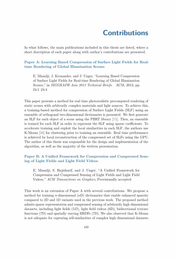
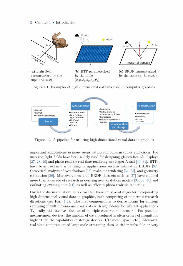
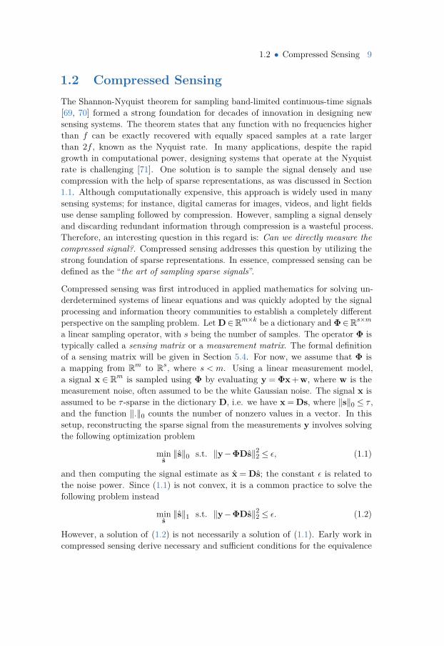
The ongoing advances in imaging techniques have introduced a range of newlarge-scale visual data such as light field images [20] and video [21], measuredBRDFs [22] and Spatially Varying BRDFs (SVBRDF) [23], multispectral images [24],Bidirectional Texture Functions (BTF) [25], and Magnetic Resonance Imaging(MRI) [26]. A common feature of these datasets is high dimensionality, see Fig.1.1. For instance, a light field is a 5D function defined as l(r, t,u,v,λ), where(r, t) describes the spatial domain, (u,v) parametrizes the angular domain, and λrepresents wavelength. A BRDF, can be parametrized as a 4D, 5D, or 6D objectdepending on the way we define the dependence on wavelengths. Recent advancesin imaging technologies enable capturing of these datasets with a high resolutionalong each dimension. Moreover, existing means for capturing such datasets canbe extended to accommodate more information, e.g. for acquiring multispectrallight field videos.
The various types of high dimensional data described above have found novel and
2 Chapter 1 • Introduction
Camera Plane
Image Plane
(u,v)
(r,t)
(a) Light fieldparameterized by thetuple (r, t,u,v)
x
y
(b) BTF parameterizedby the tuple(x,y,φi,θi,φo,θo)
n
material surface
p
(c) BRDF parameterizedby the tuple (φi,θi,φo,θo)
Figure 1.1: Examples of high dimensional datasets used in computer graphics.
•Natural
•Synthetic
•Controlled or arbitrary
Scene
•Image and video
•Light field and Light field video
•BRDF and SVBRDF
•BTF, etc.
Measurement•Resampling
•Finding a suitable transformation domain
•Compression
•Editing in transformed domain
Representation and storage
•Decompression
•Rendering
•Inverse problems
Reconstruction
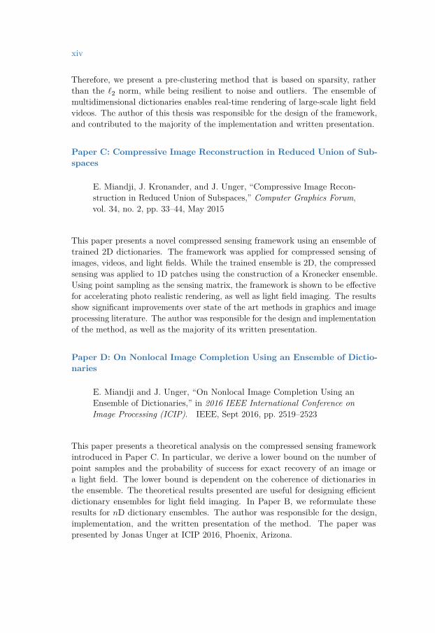
Figure 1.2: A pipeline for utilizing high dimensional visual data in graphics
important applications in many areas within computer graphics and vision. Forinstance, light fields have been widely used for designing glasses-free 3D displays[27, 28, 29] and photo-realistic real time rendering, see Paper A and [30, 31]. BTFshave been used in a wide range of applications such as estimating BRDFs [32],theoretical analysis of cast shadows [33], real-time rendering [34, 35], and geometryestimation [36]. Moreover, measured BRDF datasets such as [37] have enabledmore than a decade of research in deriving new analytical models [38, 39, 40] andevaluating existing ones [41], as well as efficient photo-realistic rendering.
Given the discussion above, it is clear that there are several stages for incorporatinghigh dimensional visual data in graphics, each comprising of numerous researchdirections (see Fig. 1.2). The first component is to derive means for efficientcapturing of multidimensional visual data with high fidelity for different applications.Typically, this involves the use of multiple cameras and sensors. For portablemeasurement devices, the amount of data produced is often orders of magnitudehigher than the capabilities of storage devices (I/O speed, space, etc.). Moreover,real-time compression of large-scale streaming data is either infeasible or very
3
costly. However, it is possible to directly measure the compressed data, which willbypass two costly stages: namely the storage of raw data followed by compression.This is the fundamental idea behind compressed sensing [42], a relatively newfield in applied mathematics and signal processing. Section 1.2 presents a briefdescription of the contributions of this thesis in the field of compressed sensing.These contributions advance the field in two fundamental areas: theoretical andempirical.
Another important aspect regarding multidimensional visual data is to find al-ternative representations of the data that facilitate storage, processing, and fastreconstruction. In order to derive suitable basis functions for efficient representationof the data, it is required to have accurate data models. An important reason forfinding transformations of the data is that the original domain of the data is toocomplicated to be analyzed, stored, or rendered. With the ever growing storagecost of these datasets and the limitations of processing power and memory, suchrepresentations have been a fundamental component in many applications sincethe early days of computer graphics. For instance, Spherical Harmonics have beenused for BRDF inference [43], and representation of radiance transfer functions [44].Fourier domain has been used for theoretical analysis of light transport [45, 46]and various other applications [47, 48, 49]. Furthermore, wavelets have also beenshown to be an important tool in graphics [50, 51, 52, 53].
Throughout this thesis, we use the word dictionary to describe a set of basisfunctions. Just like a sentence or a speech is a linear combination of words from adictionary, multidimensional visual data can be formed using a linear combinationof atoms. An atom is a basis function or a common feature in a dataset. Acollection of atoms forms a dictionary. Dictionaries can be divided into two majorgroups [54]: analytical and learning-based. Analytical dictionaries are based on amathematical model of the data, where an equation or a series of equations areused to effectively represent the data. The Fourier basis, wavelets, curvelets [55],and shearlets [56] are a few examples of dictionaries in this group. On the otherhand, machine learning techniques can be used on a large set of examples to obtaina learning-based dictionary. While learning-based dictionaries have been shownto produce better results due to their adaptivity, they are often computationallyexpensive and pose various challenges for large signal sizes.
Of particular interest in many signal and image processing applications is sparserepresentations, where a signal can be modeled by linear combination of a smallsubset of atoms in the dictionary. Since a signal is modeled using a few scalars,compression is a direct byproduct of sparse representations. Visual data such asnatural images and light fields admit sparse representations if a suitable dictionaryis given or trained. The quality of representation, i.e. the sparsity and the amountof error introduced by the model, are directly related to the dictionary. Indeed,
4 Chapter 1 • Introduction
the more sparse the representation is, the higher the compression ratio becomes.This thesis makes several contributions in this direction. In particular, we proposealgorithms that enable highly sparse representations of multidimensional visualdata, as well as various applications that utilize this model for efficient compressionof large scale datasets in graphics. The enhanced sparsity of the representationis also a key component for compressed sensing. The more sparse a signal is, theless samples are required to exactly reconstruct the signal. We briefly describe andformulate sparse representations in Section 1.1, followed by the contributions ofthis thesis on the topic.
1.1 Sparse RepresentationData models have had a central contribution during the past few decades in imageprocessing and computer graphics [57]. Fundamental problems such as sampling,denoising, super-resolution, and classification cannot be tackled effectively withoutprior assumptions about the signal model. Indeed natural visual data such as imagesand light fields contain structures and features that can be modeled effectively tofacilitate reconstruction, sampling, or even synthesizing new examples of [58, 59].If such structures did not exists, one could hope for creating an image of acat by sampling from a uniform distribution – a very unlikely outcome. Sparserepresentation is a signal model that has been successfully applied in many imageprocessing applications, ranging from solving inverse problems [60, 61, 62] to imageclassification [63, 64].
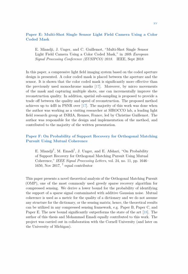
We first present an illustrative definition of sparse representation in a two dimen-sional space, followed by a general formulation of the sparse representation problem.Assume that a set of points (discrete signals) in a two dimensional space are given,see Fig. 1.3a. Indeed we need two scalars to describe the location of each point.If we rotate and translate the coordinate axes, see Fig. 1.3b, we obtain a newcoordinate system, for which the red, green, and blue points can be representedwith one scalar instead of two. We have now achieved a sparse representation forthree of the points in a new orthogonal coordinate system. In other words, we havereduced the amount of information needed to represent the points. It can be notedthat the blue point is not exactly sparse since it does not completely lie on oneof axes. This is a common outcome in practice since a large family of signals arenot exactly sparse. However, if a coordinate value is close to zero, we can assumesparsity, albeit at cost of introducing error in the representation.
In order to construct a coordinate system that admits a sparse representation forthe black point, we can add a new coordinate axis, as shown in Fig. 1.3c. Thismight seem counter-intuitive since by adding a coordinate axis we have increasedthe amount of information needed for representing the points. However, the red,

1.1 • Sparse Representation 5
(a) (b)
(c) (d)
Figure 1.3: An Illustration of (a) a set of points in a 2D space and their sparserepresentation using (b) an orthogonal dictionary, (c) an overcomplete dictionary,and (d) an ensemble of orthogonal dictionaries.
green, and blue points are already sparse. As a result, we now only need onescalar to represent each of the four points. Moreover, in practice, we have farmore points than coordinate axes. The problem of finding the smallest set ofcoordinate axes that produces the most sparse representation for all the pointsis known as dictionary learning. From the discussion above, it can deduced thateach coordinate axis is an atom in a dictionary (coordinate system). Note thatby adding the third atom in Fig 1.3c, we lost the orthogonality of the dictionary.An alternative to adding a new atom is to construct an additional orthogonaldictionary, as shown in Fig. 1.3d. The majority of the work presented in this thesisuses a set of orthogonal dictionaries for sparse representation, which we refer to asan ensemble of dictionaries.
We now formulate the sparse representation of discrete signals in Rm. Let thevector x ∈ Rm be a discrete signal, e.g. a vectorized image. The linear systemDs = x models the signal as a linear combination of k atoms (coordinate axes)that are arranged as the columns of a dictionary D ∈ Rm×k using the weights in
6 Chapter 1 • Introduction
20 40 60 80 1000
0.2
0.4
0.6
0.8
1
(a) q = 0.5
20 40 60 80 1000
0.2
0.4
0.6
0.8
1
(b) q = 1.0
20 40 60 80 1000
0.2
0.4
0.6
0.8
1
(c) q = 2.0
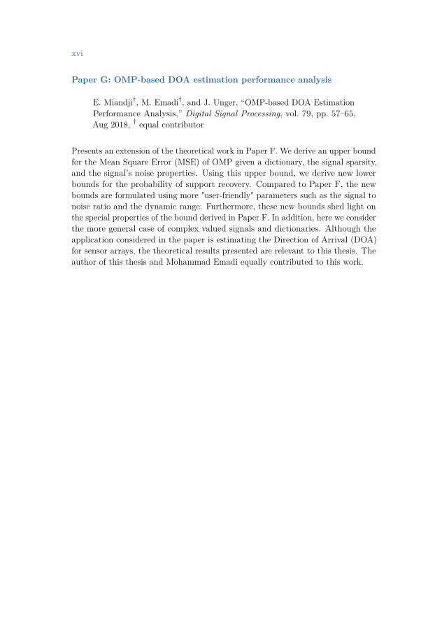
Figure 1.4: Examples of a compressible signal s ∈ R100 for C = 1 and differentvalues of q. The values of s are assumed to be sorted in decreasing order based ontheir magnitude.
Kodak parrots image
DCT
Reference 5% 10% 20% 30%
AMDE
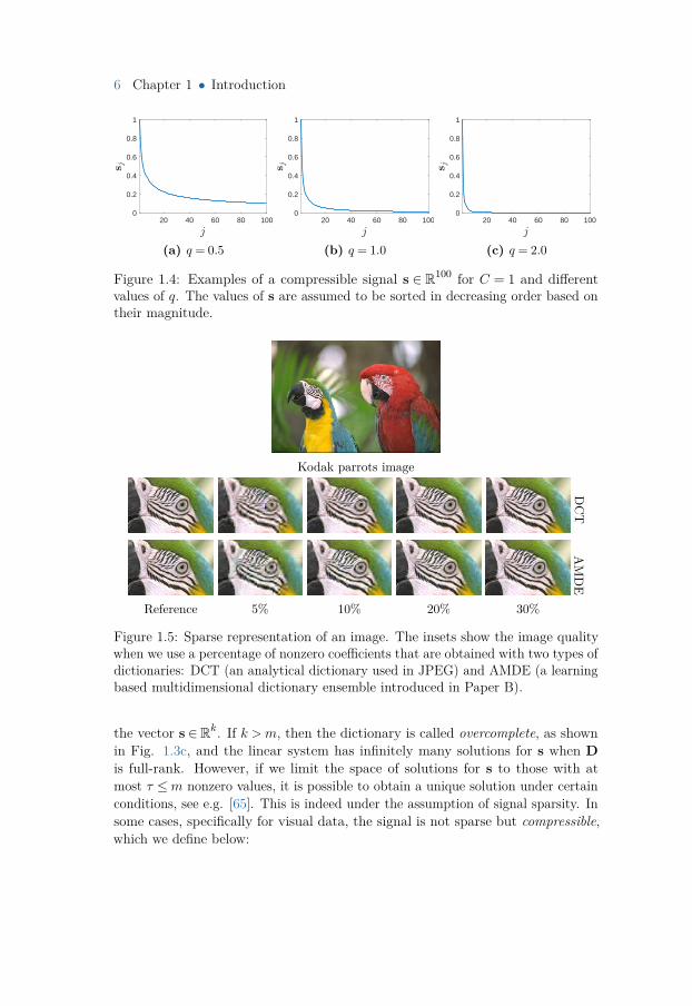
Figure 1.5: Sparse representation of an image. The insets show the image qualitywhen we use a percentage of nonzero coefficients that are obtained with two types ofdictionaries: DCT (an analytical dictionary used in JPEG) and AMDE (a learningbased multidimensional dictionary ensemble introduced in Paper B).
the vector s ∈ Rk. If k >m, then the dictionary is called overcomplete, as shownin Fig. 1.3c, and the linear system has infinitely many solutions for s when Dis full-rank. However, if we limit the space of solutions for s to those with atmost τ ≤m nonzero values, it is possible to obtain a unique solution under certainconditions, see e.g. [65]. This is indeed under the assumption of signal sparsity. Insome cases, specifically for visual data, the signal is not sparse but compressible,which we define below:
1.1 • Sparse Representation 7
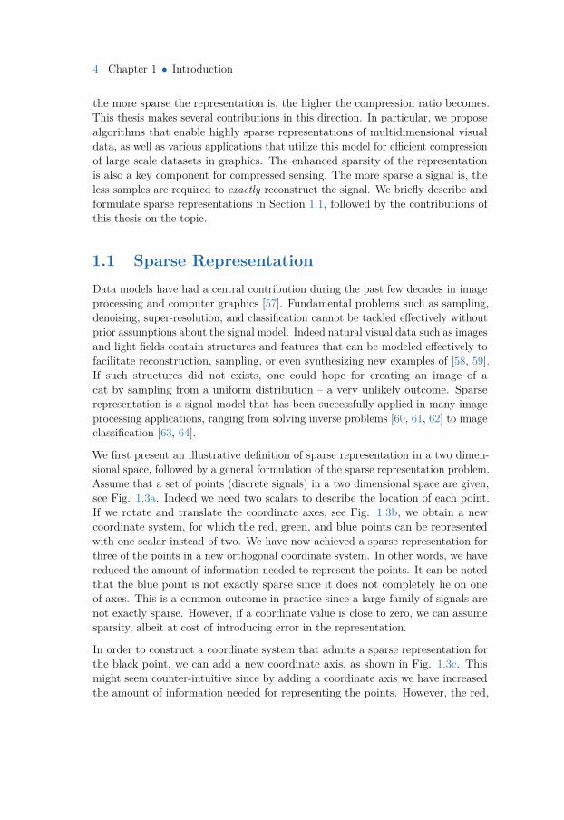
Definition 1.1 (compressible signal). A signal x ∈ Rm is called compressibleunder a dictionary D ∈ Rm×k if x = Ds and the sorted magnitude of elements in sobey the power law, i.e. |sj | ≤ Cj−q, j ∈ 1,2, . . . ,k, where C is a constant.
Examples of signals obeying the power law are given in Fig. 1.4. It is well knownthat visual data such as images, videos, light fields, etc., are compressible ratherthan sparse. In other words, the vector s is unlikely to have elements that are exactlyzero; however, the majority of elements are close to zero. Hence, a compressiblesignal can be converted to a sparse signal by nullifying the smallest elementsof the vector s. This process will indeed introduce error in the representation.Nevertheless, since the nullified elements are small in magnitude, the error istypically negligible. In Fig. 1.5, we show the effect of nullifying small coefficientsof a compressible signal (an image in this case) on the image quality. In particular,the effect of increasing τ/m, i.e. the ratio of nonzero coefficients to the signallength, on image quality is shown. Indeed having more nonzero coefficients leads toa higher image quality while increasing the storage complexity. Moreover, havingmore nonzero coefficients requires more samples when we would like to sample asparse signal, see Section 1.2 for more details.
Sparse representation can be defined as the problem of finding the most sparse set ofcoefficients for a given signal with minimal error. When an analytical overcompletedictionary is given, sparse representation amounts to solving a least squares problemwith a constraint on the sparsity or the representation error. However, we alsoneed to find a suitable dictionary that enables sparse representation. As mentionedearlier in this chapter, one approach is to construct a dictionary from a set ofexamples using machine learning, which will be described in more detail in Section2.4. Therefore, to obtain the most sparse representation of a set of signals, wehave two unknowns: 1. the dictionary and 2. the set of sparse coefficients.Estimating each of these entities requires an estimate of the other. Therefore, it isa common practice to solve this problem by alternating between the estimationof the coefficients and the dictionary, which is a fundamental problem in sparserepresentation. Perhaps the most eloquent description of this fundamental problemis given by A. M. Bruckstein in the Foreword of the first book on the topic [66]:
“The field of sparse representations, that recently underwent a Big-Bang-like expansion, explicitly deals with the Yin-Yang interplay betweenthe parsimony of descriptions and the “language” or “dictionary” usedin them, and it became an extremely exciting area of investigation.”
This thesis makes contributions on finding suitable models for sparse representationof multidimensional visual data that promote sparsity, while reducing the represen-tation error. Sparse representation of multidimensional visual data is the topic of
8 Chapter 1 • Introduction
Chapter 3, where we describe a highly effective dictionary learning method thatenables very sparse representations with minimal error. The proposed method isutilized in a variety of applications, discussed in Chapter 4, including compressionand real time photorealistic rendering. In the remainder of this section, a briefdescription of these applications is presented.
Indeed a direct consequence of sparse representation is compression since we onlyneed to store the nonzero coefficients of a sparse signal. This has been a commonpractice for compression. For instance, the JPEG standard for compressing imagesuses an analytical dictionary, namely the Discrete Cosine Transform (DCT), toobtain and compress a set of sparse coefficients. Similarly, JPEG2000 [67] usesCDF 9/7 wavelets [68]. Recent video compression methods such as HEVC (H.265)also use a variant of DCT for compression. While analytical dictionaries are fastto evaluate, learning-based dictionaries significantly outperform them in termsof reconstruction quality and sparsity of coefficients. In this direction, Paper Apresents a method for compression of Surface Light Field (SLF) datasets generatedusing a photo-realistic renderer. The proposed algorithm relies on a trainedensemble of orthogonal dictionaries that operates on the rows and columns of eachHemispherical Radiance Distribution Function (HRDF), independently. An HRDFcontains the outgoing radiance along multiple directions at a single point on thesurface of an object. The compression method admits real-time reconstruction usingthe Graphics Processing Unit (GPU). As a result, real-time photorealistic renderingof static scenes with highly complex materials and light sources is achieved.
As described previously, visual datasets in graphics are often multidimensional.For instance, images are 2D objects while a light field video is a 6D object. Anefficient dictionary for sparse representation should accommodate datasets withdifferent dimensionality. In Paper B, a dictionary training method is presentedthat computes an ensemble of nD orthonormal dictionaries. Moreover, a novelpre-clustering method is introduced that improves the quality of the learnedensemble while substantially reducing the computational complexity. The proposedmethod can be utilized for the sparse representation, and hence the compression,of any discrete dataset in graphics and visualization, regardless of dimensionality.Moreover, the sparse representation obtained by the dictionary ensemble enablesreal time reconstruction of large-scale datasets. For instance, we demonstrate realtime rendering of high resolution light field videos on a consumer level GPU. Theindependence of the dictionaries on dimensionality admits the application of ourmethod for a wide range of datasets including videos, light fields, light field videos,BTFs, measured BRDFs, SVBRDFs, etc.
1.2 • Compressed Sensing 9
1.2 Compressed SensingThe Shannon-Nyquist theorem for sampling band-limited continuous-time signals[69, 70] formed a strong foundation for decades of innovation in designing newsensing systems. The theorem states that any function with no frequencies higherthan f can be exactly recovered with equally spaced samples at a rate largerthan 2f , known as the Nyquist rate. In many applications, despite the rapidgrowth in computational power, designing systems that operate at the Nyquistrate is challenging [71]. One solution is to sample the signal densely and usecompression with the help of sparse representations, as was discussed in Section1.1. Although computationally expensive, this approach is widely used in manysensing systems; for instance, digital cameras for images, videos, and light fieldsuse dense sampling followed by compression. However, sampling a signal denselyand discarding redundant information through compression is a wasteful process.Therefore, an interesting question in this regard is: Can we directly measure thecompressed signal?. Compressed sensing addresses this question by utilizing thestrong foundation of sparse representations. In essence, compressed sensing can bedefined as the “the art of sampling sparse signals”.
Compressed sensing was first introduced in applied mathematics for solving un-derdetermined systems of linear equations and was quickly adopted by the signalprocessing and information theory communities to establish a completely differentperspective on the sampling problem. Let D∈Rm×k be a dictionary and Φ∈Rs×m
a linear sampling operator, with s being the number of samples. The operator Φ istypically called a sensing matrix or a measurement matrix. The formal definitionof a sensing matrix will be given in Section 5.4. For now, we assume that Φ isa mapping from Rm to Rs, where s < m. Using a linear measurement model,a signal x ∈ Rm is sampled using Φ by evaluating y = Φx + w, where w is themeasurement noise, often assumed to be the white Gaussian noise. The signal x isassumed to be τ -sparse in the dictionary D, i.e. we have x = Ds, where ‖s‖0 ≤ τ ,and the function ‖.‖0 counts the number of nonzero values in a vector. In thissetup, reconstructing the sparse signal from the measurements y involves solvingthe following optimization problem
mins‖s‖0 s.t. ‖y−ΦDs‖22 ≤ ε, (1.1)
and then computing the signal estimate as x = Ds; the constant ε is related tothe noise power. Since (1.1) is not convex, it is a common practice to solve thefollowing problem instead
mins‖s‖1 s.t. ‖y−ΦDs‖22 ≤ ε. (1.2)
However, a solution of (1.2) is not necessarily a solution of (1.1). Early work incompressed sensing derive necessary and sufficient conditions for the equivalence

10 Chapter 1 • Introduction
of (1.1) and (1.2), see e.g. [72, 73, 74]. Of particular interest in designing sensingsystems is the use of random sampling matrices, Φ, due to the simplicity ofimplementation and well-studied theoretical properties. Seminal work in the field[75, 76, 77, 78] show that a signal of length m with at most τ ≤m nonzero elementscan be recovered with overwhelming probability using Gaussian or Bernoulli sensingmatrices, provided that s ≥ Cτ ln(m/τ), where C is a universal constant. Theresult is significant since the number of samples is linearly dependent on sparsity,while being logarithmically influenced by the signal length. Therefore, compressedsensing can guarantee the exact recovery of sparse signals with vastly reducednumber of measurements compared to the Nyquist rate.
Research in compressed sensing can be divided into two categories: theoreticaland empirical. Theoretical research addresses fundamental problems such as theconditions for exact recovery of sparse signals from a few samples. In this regard,there exists two research directions. Universal results consider random measurementmatrices and derive bounds that hold for every sparse signal. Moreover, thereexists algorithm-specific theoretical analysis that derive convergence conditions foralgorithms that solve (1.1) or (1.2) without any assumptions on the sensing matrix,see e.g. [79, 80, 81, 82]. Empirical research, on the other hand, apply the sparsesensing model described above for designing effective sensing systems. For instance,compressed sensing has been used for designing a digital camera with a singlepixel [83], light field imaging [17, 84, 85], light transport sensing [86], MagneticResonance Imaging (MRI) [26, 87, 88], sensor networks [89, 90], and antenna arrays[91, 92, 93].
This thesis makes contributions in both theoretical and empirical aspects of com-pressed sensing, where the former is the topic of Chapter 5, and the latter isdiscussed in Chapter 6. The methods introduced herein show the applicabilityof compressed sensing in various subjects in graphics, while also presenting atheoretical analysis of the proposed algorithms. In this regard, Paper C presentsa compressed sensing framework for recovering images, videos, and light fieldsfrom a small number of point samples. The framework utilizes an ensemble oforthogonal dictionaries trained on a collection of 2D small patches from variousdatasets. Moreover, it is shown that the method can be used for the accelerationof photorealistic rendering techniques without a noticeable degradation in imagequality.
In Paper D, we perform a theoretical analysis of the framework presented inPaper C. This novel analysis derives uniqueness conditions for the solution of (1.1)when the signal is sparse in an ensemble of 2D orthogonal dictionaries. In otherwords, we show the required conditions for exact recovery of an image, light field,or any type of visual data from what appears to be a highly insufficient numberof samples. The main result is a lower bound on the required number of samples
1.3 • Thesis outline 11
and a lower bound on the probability of exact recovery. These theoretical resultsare reformulated in Paper B, where we consider an ensemble of nD orthogonaldictionaries. The theoretical analysis provides insight into training more efficientmultidimensional dictionaries, as well as designing effective capturing devices forlight fields, BRDFs, etc. Additionally, in Paper E we propose a new light fieldcamera design based on compressed sensing. By placing a random color codedmask in front the sensor of a consumer level digital camera, high quality and highresolution light fields can be captured.
As mentioned earlier, theoretical results on deriving optimality conditions for sparserecovery algorithms play an important role in compressed sensing. Understandingthe behaviour of a sparse recovery algorithm with respect to the properties of theinput signal, as well as the dictionary, greatly improves the design of novel sensingsystems. For instance, in designing a compressive light field camera, parameterssuch as Signal to Noise Ratio (SNR), Dynamic Range (DR), and the propertiesof the sensing matrix (which is directly coupled with the design of the camera),play an important role in efficiency and flexibility of the system. In this direction,Paper F presents a theoretical analysis of Orthogonal Matching Pursuit (OMP), agreedy algorithm that is widely used for solving (1.1). We derive a lower boundfor the probability of correctly identifying the location of nonzero entries (knownas support) in a sparse vector. Unlike previous work, this new bound takes intoaccount signal parameters, which as described earlier are important in practicalapplications. In Paper G, we extend these results by deriving an upper bound onthe error of the estimated sparse vector (i.e. the result of solving (1.1)). Moreover,by combining the probability and error bounds, we derive new “user-friendly”bounds for the probability of successful support recovery. These new bounds shedlight on the effect of various parameters for compressed sensing using OMP.
1.3 Thesis outlineThe thesis is divided into two parts. The first part introduces background theoryand gives an overview of the contributions presented in this thesis. The secondpart is a compilation of seven selected publications that provide more detaileddescriptions of the research leading up to this thesis.
The first part of this thesis is divided into six chapters. As the title of this thesissuggests, our main focus is on compression and compressed sensing of visual data bythe means of effective methods for sparse representations. In Chapter 2, importanttopics that lay the foundation of this thesis will be presented. Specifically, wediscuss multi-linear algebra (utilized in Paper B), algorithms for recovery of sparsesignals (used in all the included papers except for Paper A), dictionary learning(utilized in Paper A, Paper B, Paper C, Paper D, and Paper E), and different types
12 Chapter 1 • Introduction
of visual data, as well as the challenges and opportunities that are associated withthem. Chapter 3 will present novel techniques for efficient sparse representation ofmultidimensional visual data, followed by a number of applications in computergraphics that utilize these techniques for compression in Chapter 4. In Chapter 5 werevisit compressed sensing, which was briefly described in Section 1.2, and presentfundamental concepts regarding the theory of sampling sparse signals. Then, thetheoretical contributions of this thesis on compressed sensing will be presented.In Chapter 6, we discuss the applications of compressed sensing in graphics andimaging. A number of contributions such as light field imaging, photorealisticrendering, light field video sensing, and efficient BRDF capturing will be presented.
Each chapter will present the main contributions of this thesis on the topic, where wefirst present some background information, motivations, and how the contributionsof the author address the limitations of current methods. We conclude each chapterwith a short summary and a discussion of possible venues for future work on thetopic. Finally, in Chapter 7 we summarize the materials presented in thesis andprovide an outlook on the future of the field of sparse representations, in connectionto compression and compressed sensing, for efficient acquisition, storage, processing,and rendering of visual data. We pose several research questions that will hopefullyprovide new directions for future research.
1.4 Aim and ScopeThe aim of the research conducted by the author and presented in this thesishas been to derive methods and frameworks that are applicable to many differentdatasets utilized in computer graphics and image processing. While the mainfocus of the empirical results presented here is on light fields and light field videos,the compression and compressed sensing methods introduced in this thesis areapplicable to BRDF, SVBRDF, BTF, light transport data, and hyper-spectraldata, as well as new types of high dimensional datasets that are to appear in thefuture. The theoretical results of Paper D, Paper F, and Paper G have even a widerscope in terms of applicability in different areas of research on compressed sensing.Indeed any compressed sensing framework based on an overcomplete dictionaryor an ensemble of dictionaries can utilize these results. More importantly, thetheoretical results presented here can be used to guide the design of new sensingsystems for efficient capturing of multidimensional visual data.
As mentioned earlier, a substantial part of the thesis discusses sparse representationsfor compression of visual data. However, transform coding by the means of sparserepresentations is typically a small part of a full compression pipeline. For instance,the JPEG standard uses Huffman coding [94] to further compress the sparsecoefficients obtained from a DCT dictionary. Moreover, the HEVC codec uses a

1.4 • Aim and Scope 13
series of advanced coding algorithms in different stages to reduce the redundancyof data in time domain. Therefore, although the term “compression” is used inthis thesis, we only address the problem of finding the most sparse representationof visual data, and the coding of sparse coefficient is out of the scope of the thesis.However, it should be noted that any type of entropy coding technique can beimplemented on top of algorithms we present here.


Ch
ap
te
r
2Preliminaries
In this Chapter, important topics that are utilized throughout this thesis will bediscussed. We start by describing the mathematical notations used throughout thisthesis in Section 2.1. Tensor algebra and methods for tensor approximations arepresented in Section 2.2. In particular, we present simple operations on tensors andintroduce Higher Order SVD (HOSVD), which has been widely used in computergraphics and image processing applications. Next, the sparse signal estimation isformulated in Section 2.3. Two major approaches for addressing this problem, i.e.greedy and convex relaxation methods, are discussed. Additionally, an extensiveliterature review of existing methods is presented. We also discuss some of therecent advances in solving the high dimensional variant of the problem. In Section2.4, we formulate and discuss various methods for dictionary learning. We start bypresenting the most commonly used dictionary learning method (K-SVD). Thena comprehensive review of existing methods is presented. Moreover, the highdimensional dictionary learning problem is formulated and recent methods forsolving it are discussed. Finally, a short description of common types of visualdata in computer graphics are presented in Section 2.5. Additionally, we discussthe challenges and opportunities associated with the capturing, storage, and therendering of these datasets.
2.1 NotationsThroughout this thesis, the following notational convention is used. Vectors andmatrices are denoted by boldface lower-case (a) and bold-face upper-case letters
16 Chapter 2 • Preliminaries
(A), respectively. Tensors are denoted by boldface calligraphic letters, e.g. A.A finite set of objects is indexed by superscripts, e.g.
A(i)N
i=1orA(i)N
i=1.
In some cases, for convenience, we may use multiple indices for these sets, e.g.A(i,j)N,M
i=1,j=1. Individual elements of a, A, andA are denoted ai, Ai1,i2 , Ai1,...,iN ,
respectively. The ith column and row of A are denoted Ai and Ai,:, respectively.Similarly, the jth tensor fiber is denoted by Ai1,i2,...,ij−1,:,ij+1,...,iN . The functionvec(A) performs vectorization of its argument; e.g. the elements of a tensor alongrows, columns, depth, etc. are arranged in a vector. Given an index set, I, thesub-matrix AI is formed from columns of A indexed by I. The N-mode productof a tensor with a matrix is denoted by ×N , e.g. X ×N B. The Kronecker productof two matrices is denoted A⊗B and the outer product of two vectors is denoteda b.
The `p norm of a vector s, for 1≤ p≤∞, is denoted by ‖s‖p. The induced operatornorm for a matrix is denoted ‖A‖p. By definition we have ‖A‖2 = λmax(A), whereλmax(.) denotes the largest singular value of a matrix (in absolute value). Frobeniusnorm of a matrix is denoted ‖A‖F . The `0 pseudo-norm of a vector, denoted ‖s‖0,defines the number of non-zero elements. The location of non-zero elements in s,also known as the support set, is denoted supp(s). Consequently, ‖s‖0 = |supp(s)|,where |.| denotes set cardinality. Occasionally, the exponential function, ex, isdenoted exp(x). Moore-Penrose inverse of a matrix is denoted A†. Probabilityof an event B is denoted PrB and the expected value of a random variable xis shown as Ex. For defining a variable, we use the symbol =∆ ; for instance,C =∆ A⊗B.
2.2 Tensor ApproximationsThe term “tensor” is indeed an ambiguous term with various definitions in differentfields of science and engineering. The main definition of a tensor comes fromthe field of differential geometry. A tensor is an invariant geometric object thatdoes not depend on the choice of the local coordinate system on a manifold. Inparticular, a tensor of type (p,q) of rank p+q is an object defined in each coordinatesystem x(i)ni=1 by the set of numbers T i1,...,ip
j1,...,jqsuch that a coordinate substitution
x(i)ni=1→y(i′)ni′=1 is according to the law [95]
T i′1,...,i
′p
j′1,...,j
′q
= ∂y(i′1)
∂x(i1) . . .∂y(i′p)
∂x(ip)∂x(j1)
∂y(j′1). . .
∂x(jq)
∂y(j′q)T i1,...,ipj1,...,jq
, (2.1)
where we have used the Einstein summation convention. Tensor algebra was themain mathematical tool in deriving the theory of general relativity. In the fields ofcomputer graphics and image processing, the term tensor is often used to define
2.2 • Tensor Approximations 17
higher-order matrices, also known as multidimensional arrays. This definition doesnot necessarily consider the transformation law in (2.1), and is only defined inRn. We also follow this convention, i.e. the term “tensor” in this thesis refers to amultidimensional array of scalars.
Tensors are omnipresent in various applications such as computer graphics [96, 97,98, 99, 100], imaging techniques [101, 102, 103, 104], image processing and computervision [105, 106, 107, 108], as well as scientific visualization [109, 110, 111]. Whiletensors are merely an extension of matrices to dimensions larger than two, many ofthe tools used in matrix analysis are not applicable to tensors. In what follows, abrief description of a few tensor operations, e.g. unfolding and decomposition, willbe presented. Note that the concepts relevant to this thesis will be covered and formore details the reader is referred to a comprehensive review article by Kolda andBader [112] and a book on the topic [113].
Let X ∈ Rm1×m2×···×mn be a real-valued n-dimensional (nD) tensor, also referredto as an n-way or n-mode tensor. The values along a certain mode of a tensor iscalled a fiber. For instance, second mode fibers of a 3D tensor Z ∈ Rm1×m2×m3
are obtained from Zi1,:,i3 for different values of i1 and i3.
The norm of a tensor X is calculated as
‖X‖=
√√√√√ m1∑i1=1
m2∑i2=1
. . .mn∑in=1
X 2i1,i2,...,in . (2.2)
Multiplication of a tensor with a matrix along mode N is called the N -modeproduct and is denoted by the symbol ×N . Given a tensor X ∈Rm1×m2×···×mn anda matrix U ∈ RJ×mN , the result of the N -mode product is a tensor of dimensionm1× . . .mN−1×J×mN+1×·· ·×mn with elements
(X ×N U)i1,...,iN−1,j,iN+1,...,in =mN∑iN=1
Xi1,i2,...,iN−1,iN ,iN+1,...,inUj,iN. (2.3)
Another useful operation on tensors is unfolding, also known as flattening ormatricization. This operation transforms a tensor into a matrix by taking the fibersalong a certain mode of the tensor and arranging them as columns of a matrix.The unfolding of a tensor X along mode N is denoted X(N). In this process, anelement Xi1,i2,...,iN−1,iN ,iN+1,...,in maps to a matrix element X(N)(iN , j), where
j = 1 +n∑
k=1, k 6=N
(ik−1)k−1∏
p=1, p6=Nmp
. (2.4)
Tensor unfolding allows us to use well-established tools from matrix analysison tensors. For instance, N -mode product can be mapped to a matrix-matrix
18 Chapter 2 • Preliminaries
multiplication using unfolding:
Y = X ×N U ⇔ Y(N) = UX(N), (2.5)
where Y can be obtained by folding Y(N) (i.e. by performing the inverse ofunfolding).
The nD tensor X is rank one if it can be written as X = a(1) a(2) · · ·a(n), wherea(i) ∈ Rmi and the symbol denotes the outer product of vectors. Moreover, therank of X is the smallest positive integer R such that
X =R∑r=1
a(r,1) a(r,2) · · · a(r,n). (2.6)
Calculating the rank of a tensor is NP-hard. This is in contrast with the rank ofa matrix, which is uniquely defined and can be obtained by e.g. Singular ValueDecomposition (SVD).
The tensor rank decomposition in (2.6) is known as the CANDECOMP/PARAFACdecomposition, or CP in short. While CP decomposition requires weaker conditionsfor uniqueness [114] (in contrast to matrix rank decompositions), it is typicallyintractable to compute. This is because R is unknown and an algorithm that solves(2.6) for a fixed R remains an active research problem [115, 116, 117, 118, 119, 120].Another tensor decomposition method that has been widely used in many scientificand engineering problems is the Higher Order SVD (HOSVD) [121], also known asthe Tucker decomposition. The HOSVD of the tensor X is as follows
X = G×1 U(1)×2 U(2)×3 · · ·×nU(n), (2.7)
where G is called a core tensor and the matrices U(i)ni=1 are orthogonal (oftenorthonormal). It is possible to obtain a truncated HOSVD by only computing afraction of columns of U(i)ni=1. In this way, G becomes a compressed version of X .Alternatively, one can set the small values of G to zero to achieve compression of X .It should be noted that unlike truncated SVD of matrices, truncated HOSVD is notnecessarily optimal in an `2 sense. However, computing HOSVD is straightforward,see Algorithm 1.
While the result of HOSVD is not necessarily optimal, it is typically used as astarting point for iterative algorithms such as Alternating Least Squares (ALS)[115].
In some applications, it is more convenient to use the matrix representation of theN -mode product. This enables the utilization of existing tools in matrix analysis.
2.3 • Sparse Signal Estimation 19
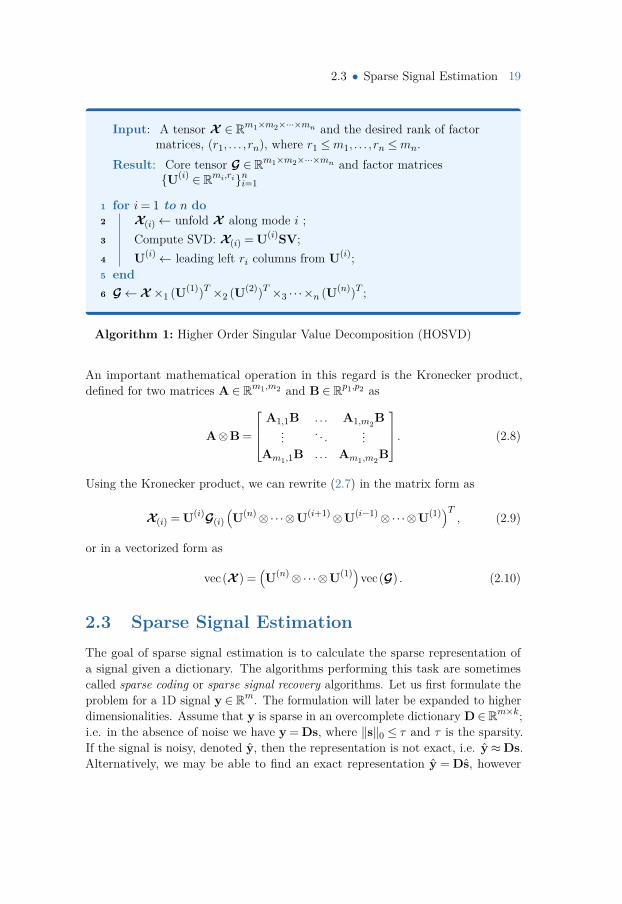
Input: A tensor X ∈ Rm1×m2×···×mn and the desired rank of factormatrices, (r1, . . . , rn), where r1 ≤m1, . . . , rn ≤mn.
Result: Core tensor G ∈ Rm1×m2×···×mn and factor matricesU(i) ∈ Rmi,rini=1
1 for i= 1 to n do2 X(i)← unfold X along mode i ;3 Compute SVD: X(i) = U(i)SV;4 U(i)← leading left ri columns from U(i);5 end6 G←X ×1 (U(1))T ×2 (U(2))T ×3 · · ·×n (U(n))T ;
Algorithm 1: Higher Order Singular Value Decomposition (HOSVD)
An important mathematical operation in this regard is the Kronecker product,defined for two matrices A ∈ Rm1,m2 and B ∈ Rp1,p2 as
A⊗B =
A1,1B . . . A1,m2B... . . . ...
Am1,1B . . . Am1,m2B
. (2.8)
Using the Kronecker product, we can rewrite (2.7) in the matrix form as
X(i) = U(i)G(i)(U(n)⊗·· ·⊗U(i+1)⊗U(i−1)⊗·· ·⊗U(1))T , (2.9)
or in a vectorized form as
vec(X ) =(U(n)⊗·· ·⊗U(1))vec(G) . (2.10)
2.3 Sparse Signal EstimationThe goal of sparse signal estimation is to calculate the sparse representation ofa signal given a dictionary. The algorithms performing this task are sometimescalled sparse coding or sparse signal recovery algorithms. Let us first formulate theproblem for a 1D signal y ∈ Rm. The formulation will later be expanded to higherdimensionalities. Assume that y is sparse in an overcomplete dictionary D ∈Rm×k;i.e. in the absence of noise we have y = Ds, where ‖s‖0 ≤ τ and τ is the sparsity.If the signal is noisy, denoted y, then the representation is not exact, i.e. y≈Ds.Alternatively, we may be able to find an exact representation y = Ds, however
20 Chapter 2 • Preliminaries
at the cost of reducing sparsity, i.e. ‖s‖0 ≥ ‖s‖0. The sparse signal estimation isformulated as follows
mins ‖s‖0 s.t. ‖y−Ds‖22 ≤ ε, (2.11)
where an estimate of noise is required to set the value of ε. If we have an estimateof sparsity, we may solve
mins ‖y−Ds‖22 s.t. ‖s‖0 ≤ τ. (2.12)
When neither τ nor ε can be estimated, the unconstrained problem (i.e. theLagrangian form) is solved
mins λ‖s‖0 + 12‖y−Ds‖22. (2.13)
Equation (2.13) is known as the Basis Pursuit DeNoising (BPDN) [122]. Solvingthe above problems is NP-hard due to non-convexity of the `0 norm. The maindifficulty arises from the fact that we do not know the location of nonzero values ins. Let us define the function supp(s), which outputs the location of nonzero valuesas an index set, known as the support of a sparse signal. In fact, if the support ofs is known, then (2.11) reduces to a least squares problem with the closed-formsolution sΛ = D†Λy,
s1,...,k\Λ = 0,(2.14)
where the operator \ denotes set difference. However, the support of s is in generalunknown and as of writing this thesis, there is no algorithm other than an exhaustivesearch over all possible support sets; i.e. one has to solve
(kτ
)least squares problems,
assuming that we know the sparsity of the solution. As an example, finding thesupport for an image of size 32×32 that is sparse, with τ = 16, under a dictionaryD ∈ R1024×2048 will take approximately 1.37e+22 years to complete if each leastsquares problem takes 1.0e−10 of a second!
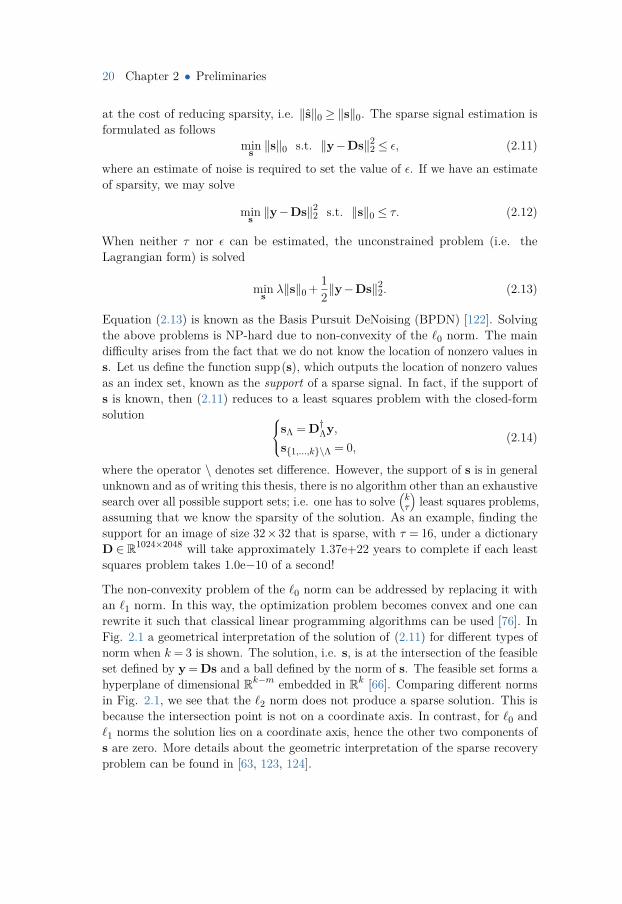
The non-convexity problem of the `0 norm can be addressed by replacing it withan `1 norm. In this way, the optimization problem becomes convex and one canrewrite it such that classical linear programming algorithms can be used [76]. InFig. 2.1 a geometrical interpretation of the solution of (2.11) for different types ofnorm when k = 3 is shown. The solution, i.e. s, is at the intersection of the feasibleset defined by y = Ds and a ball defined by the norm of s. The feasible set forms ahyperplane of dimensional Rk−m embedded in Rk [66]. Comparing different normsin Fig. 2.1, we see that the `2 norm does not produce a sparse solution. This isbecause the intersection point is not on a coordinate axis. In contrast, for `0 and`1 norms the solution lies on a coordinate axis, hence the other two components ofs are zero. More details about the geometric interpretation of the sparse recoveryproblem can be found in [63, 123, 124].
2.3 • Sparse Signal Estimation 21
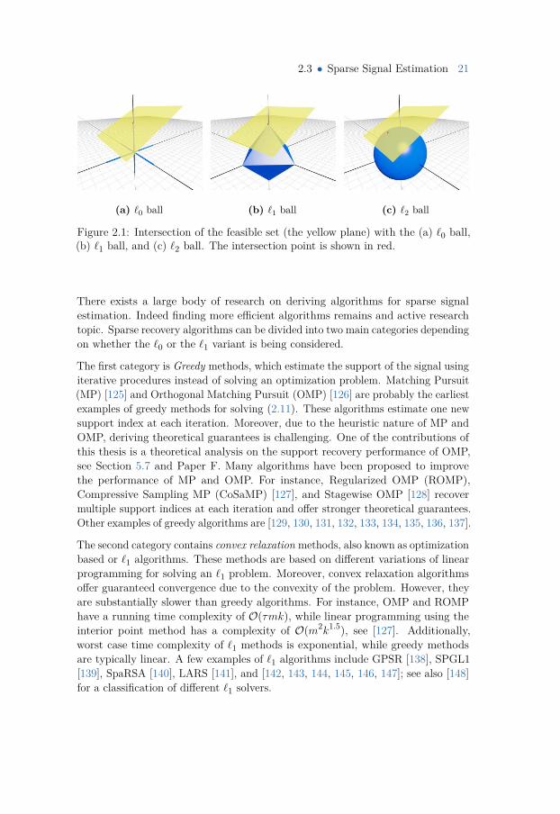
(a) `0 ball (b) `1 ball (c) `2 ball
Figure 2.1: Intersection of the feasible set (the yellow plane) with the (a) `0 ball,(b) `1 ball, and (c) `2 ball. The intersection point is shown in red.
There exists a large body of research on deriving algorithms for sparse signalestimation. Indeed finding more efficient algorithms remains and active researchtopic. Sparse recovery algorithms can be divided into two main categories dependingon whether the `0 or the `1 variant is being considered.
The first category is Greedy methods, which estimate the support of the signal usingiterative procedures instead of solving an optimization problem. Matching Pursuit(MP) [125] and Orthogonal Matching Pursuit (OMP) [126] are probably the earliestexamples of greedy methods for solving (2.11). These algorithms estimate one newsupport index at each iteration. Moreover, due to the heuristic nature of MP andOMP, deriving theoretical guarantees is challenging. One of the contributions ofthis thesis is a theoretical analysis on the support recovery performance of OMP,see Section 5.7 and Paper F. Many algorithms have been proposed to improvethe performance of MP and OMP. For instance, Regularized OMP (ROMP),Compressive Sampling MP (CoSaMP) [127], and Stagewise OMP [128] recovermultiple support indices at each iteration and offer stronger theoretical guarantees.Other examples of greedy algorithms are [129, 130, 131, 132, 133, 134, 135, 136, 137].
The second category contains convex relaxation methods, also known as optimizationbased or `1 algorithms. These methods are based on different variations of linearprogramming for solving an `1 problem. Moreover, convex relaxation algorithmsoffer guaranteed convergence due to the convexity of the problem. However, theyare substantially slower than greedy algorithms. For instance, OMP and ROMPhave a running time complexity of O(τmk), while linear programming using theinterior point method has a complexity of O(m2k1.5), see [127]. Additionally,worst case time complexity of `1 methods is exponential, while greedy methodsare typically linear. A few examples of `1 algorithms include GPSR [138], SPGL1[139], SpaRSA [140], LARS [141], and [142, 143, 144, 145, 146, 147]; see also [148]for a classification of different `1 solvers.
22 Chapter 2 • Preliminaries
Apart from the two categories described above, there exists a “hybrid” family ofmethods. For instance, Smoothed-`0 (SL0) [82] approximates the `0 pseudo-normwith a continuous function controlled by a parameter α that converges to the `0pseudo-norm when α→ 0. While the method directly solves the `0 problem, it isbased on gradient descent instead of a greedy algorithm. Other examples of hybridmethods include [149, 150, 151, 152, 153, 154, 155].
All of the algorithms mentioned above solve a sparse recovery problem for a vector,i.e. a 1D signal. While sparse recovery of 1D signals have received a lot of attentionduring the last two decades, recovery of high dimensional signals, i.e. tensors,have been relatively untouched. Caiafa and Cichocki propose the Kronecker-OMPalgorithm [102, 156], a modification of the OMP method for tensors. Moreover,they also propose N-BOMP, an algorithm designed for block-sparse [157] tensors.In [158], the authors solve a nonlinear problem with the assumption of low rankor sparse structures along each mode. Moreover, a recovery method for low-rank tensors synthesized as sums of outer products of sparse loading vectors wasproposed in [159]; however, the algorithm relies on solving the NP-hard problem ofestimating the tensor rank. More recently, Friedland et al. proposed GeneralizedTensor Compressed Sensing (GTCS) [160]. The method is shown to be vastlysuperior in computational complexity compared to vectorized sparse recovery butsuffers from poor reconstruction quality in real world applications [161].
2.4 Dictionary Learning
The goal of dictionary learning is to construct a set of basis functions using machinelearning such that any input signal can be modeled as a linear combination ofa small subset of basis functions with the least amount of error. Just like anymachine learning method, one needs a large training set that is representative ofthe signal family being considered (e.g. a large number of images). If the trainingset does not capture different variations of the data, sparse representation of theunobserved test signals leads to low sparsity, or large error, or both.
Since sparse representation is the goal of dictionary learning, one needs an algorithmfor sparse recovery as described in Section 2.3. On the other hand, the dictionaryis a parameter in the sparse recovery problem, see (2.11). In such “chicken-and-egg”problems, it is a common practice to iteratively solve an optimization problemfor one of the parameters while fixing the other until the convergence of bothparameters. For instance, one can start by a random initialization of the dictionary,solve for the sparse coefficients, update the dictionary, and so on.
Perhaps the most commonly used dictionary learning method is K-SVD [162].Moreover, this algorithm is typically used as a baseline for evaluating the effective-
2.4 • Dictionary Learning 23
ness of dictionary learning methods. Since a large family of algorithms follow thesame steps as K-SVD, albeit with different approaches for solving the problem,we start by describing this method. The K-SVD algorithm solves the followingoptimization problem
minS,D‖X−DS‖22 s.t. ‖Si‖0 ≤ τ, ∀i ∈ 1, . . . ,N, (2.15)
where X ∈ Rm×N is a collection of N training signals, and τ is a user-definedsparsity parameter; moreover, D ∈ Rm×k and S ∈ Rk×N are the dictionary andsparse coefficients that we would like to estimate, respectively. A dictionary withk >m is called overcomplete. The larger the number of columns in D, the higherthe sparsity of the representation. A dictionary that can model a larger group ofsignals with high sparsity and low error is called representative. While increasing kleads to a more representative dictionary, it comes at the cost of significantly highercomputational cost per iteration and a slower convergence. Moreover, increasingthe overcompleteness requires a larger training set. It is common to use k = δm,where δ is a scalar defining overcompleteness. For instance, if δ = 2, we call thedictionary two times overcomplete.
K-SVD iterates over two steps until convergence: 1. sparse coding and 2. dictionaryupdate. The sparse coding is done using OMP for each signal in the training set bysolving
minSi‖Xi−DSi‖22 s.t. ‖Si‖0 ≤ τ. (2.16)
Alternatively, equation (2.16) can be solved using Batch-OMP [163] because D isfixed for all Xi.
The dictionary update is done one atom at a time, i.e. by fixing all the atomsexcept one. In order to isolate the ith atom for updating, we can rewrite theobjective function of (2.15) as
‖X−DS‖22 = ‖E(i)−DiSi,.‖22, where E(i) = X−m∑
j=1, j 6=iDjSj,., (2.17)
The vector Si,. ∈RN is the ith row of S and describes which signals in the trainingset use the ith atom. The term E(i) is a residual term that we would like to estimateusing atom i. Indeed the solution of (2.17) is obtained by a rank one approximationof E(i) using SVD. However, in this way Si,. will not fulfill the sparsity requirement.To account for the fact that we seek a sparse coefficient matrix S, we limit (2.17)to the elements of E(i) and Si,. that are in the support set of Si,.; i.e. we onlyupdate the nonzero values of Si,., which means only the signals that use the atom i
contribute to updating it. This can be simply achieved by multiplying (2.17) with
24 Chapter 2 • Preliminaries
a sampling matrix that samples elements according to supp(Si,.
). Hence, equation
(2.17) becomes
‖E(i)−DiSi,.‖22 ∝ ‖E(i)Ω(i)−DiSi,.Ω(i)‖22 = ‖Υ−Diρ
(i)‖22, (2.18)
where Υ = E(i)Ω(i) and ρ(i) = Si,.Ω(i). We can now compute a rank one SVD as
follows Υ = σuvT , and the minimizer of (2.18) is obtained by setting Di = u andρ(i) = σv.
Since the advent of K-SVD, signal and image processing communities have beenactively reporting new and improved dictionary learning methods. Online dictionarylearning [164] uses stochastic optimization techniques to significantly acceleratethe performance of K-SVD. An `1 variant of K-SVD was proposed in [165] byadopting a probabilistic approach. A different approach for solving (2.15) wasintroduced in [166] that uses majorization optimization approach, with guaranteedconvergence. Mailhé et al. propose INK-SVD by introducing an intermediatestep in K-SVD that decorrelates dictionary atoms. Low coherence leads to animproved compressed sensing performance, see Chapter 5. The proposed methodwas improved in [167]. A method for training dictionaries that are invariant underrotation and flipping was proposed in [168]. However, the method learns theinvariance for a pre-defined set of transforms. A different criteria for dictionarylearning was proposed in [169], where instead of minimizing the sparsity, a lowentropy representation is sought for compression. An extension of K-SVD to handleadditive sparse corruptions of training signals was proposed in [170]. A modificationof K-SVD was discussed in [171], where similar sparsity for individual signals ispromoted rather than a global sparsity as in (2.15). Another enhancement ofK-SVD comes in the form of adaptively determining the required number of atomsduring training [172, 173, 174, 175].
There exists a family of “task-driven” dictionary learning methods that tune thedictionary for a specific task, e.g. classification and clustering [176, 177, 178, 179,180, 181, 182], image denoising [183, 184, 185, 186], medical imaging [187, 188, 189],plenoptic imaging [190], or even reducing the block artifacts of JPEG images [191].In [192], the authors propose a variant of K-SVD where only the dictionary updateis performed. Moreover, unlike (2.18) where only the coefficients in the support areupdated, the new method updates the entire vector Si,., hence admitting the changeof support in each iteration. A divide-and-conquer method was used in [193] to traindictionaries for correlated training examples, followed by a method for combiningthe atoms. In [194], an algorithm for directly solving (2.15) without an alternatingapproach is presented; however, the performance of the proposed method is notcompetitive with K-SVD [195]. Liang et al. [196] propose a distributed algorithmto learn a dictionary over multiple nodes that can be used in a sensor network
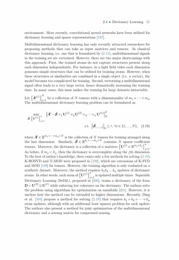
2.4 • Dictionary Learning 25
environment. More recently, convolutional neural networks have been utilized fordictionary learning and sparse representations [197].
Multidimensional dictionary learning has only recently attracted researchers forproposing methods that can take as input matrices and tensors. In classicaldictionary learning, i.e. one that is formulated by (2.15), multidimensional signalsin the training set are vectorized. However, there are two major shortcomings withthis approach. First, the trained atoms do not capture structures present alongeach dimension independently. For instance, in a light field video each dimensionpossesses simple structures that can be utilized for training atoms. However, whenthese structures or similarities are combined in a single object (i.e. a vector), themodel becomes too complicated for training. Second, vectorizing a multidimensionalsignal often leads to a very large vector, hence dramatically increasing the trainingtime. In many cases, this issue makes the training for large datasets intractable.
LetX (i)N
i=1be a collection of N tensors with a dimensionality of m1×·· ·×mn.
The multidimensional dictionary learning problem can be formulated as
minS,
U(j)nj=1
∥∥∥X − S×1 U(1)×2 U(2)×3 · · ·×nU(n)∥∥∥2
F
s.t.∥∥∥S:,...,:,i
∥∥∥0≤ τ, ∀i ∈ 1, . . . ,N, (2.19)
where X ∈Rm1×···×mn×N is the collection of N tensors for training arranged alongthe last dimension. Similarly, S ∈ Rk1×···×kn×N contains N sparse coefficienttensors. Moreover, the dictionary is a collection of n matrices
U(j) ∈ Rmj×kj
nj=1
.As before, if mj < kj , then the dictionary is overcomplete along the jth dimension.To the best of author’s knowledge, there exists only a few methods for solving (2.19).K-HOSVD and T-MOD were proposed in [198], which are extensions of K-SVDand MOD [199] for tensors. However, the training algorithm is only evaluated on asynthetic dataset. Moreover, the method requires k1k2 . . .kn updates of dictionaryatoms. In other words, each atom of
U(j)n
j=1is updated multiple times. Separable
Dictionary Learning (SeDiL), proposed in [200], trains a dictionary of the formD = U(2)⊗U(1) while enforcing low coherence on the dictionary. The authors solvethe problem using algorithms for optimization on manifolds [201]. However, it isunclear how the method can be extended to higher dimensions. Recently, Dinget al. [104] propose a method for solving (2.19) that requires k1 + k2 + · · ·+ knatom updates, although with an additional least squares problem for each update.The authors also present a method for joint optimization of the multidimensionaldictionary and a sensing matrix for compressed sensing.
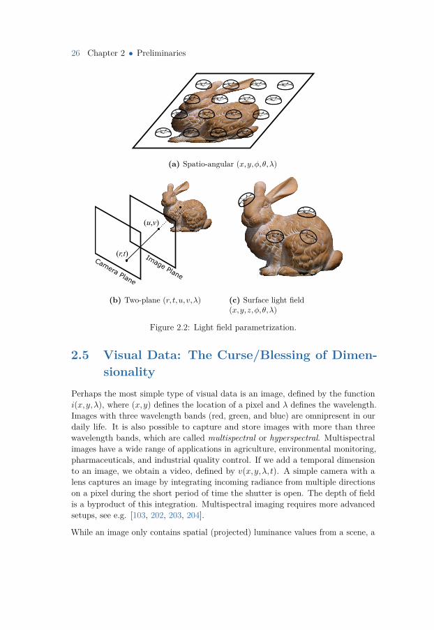
26 Chapter 2 • Preliminaries
(a) Spatio-angular (x,y,φ,θ,λ)
Camera Plane
Image Plane
(u,v)
(r,t)
(b) Two-plane (r, t,u,v,λ) (c) Surface light field(x,y,z,φ,θ,λ)
Figure 2.2: Light field parametrization.
2.5 Visual Data: The Curse/Blessing of Dimen-sionality
Perhaps the most simple type of visual data is an image, defined by the functioni(x,y,λ), where (x,y) defines the location of a pixel and λ defines the wavelength.Images with three wavelength bands (red, green, and blue) are omnipresent in ourdaily life. It is also possible to capture and store images with more than threewavelength bands, which are called multispectral or hyperspectral. Multispectralimages have a wide range of applications in agriculture, environmental monitoring,pharmaceuticals, and industrial quality control. If we add a temporal dimensionto an image, we obtain a video, defined by v(x,y,λ, t). A simple camera with alens captures an image by integrating incoming radiance from multiple directionson a pixel during the short period of time the shutter is open. The depth of fieldis a byproduct of this integration. Multispectral imaging requires more advancedsetups, see e.g. [103, 202, 203, 204].
While an image only contains spatial (projected) luminance values from a scene, a
2.5 • Visual Data: The Curse/Blessing of Dimensionality 27
light field contains both spatial and angular information. If we define a light fieldon a plane, just like an image, then each pixel has multiple values corresponding tooutgoing radiance along directions defined by a hemisphere centered at the pixel.This can be described by the function l(x,y,φ,θ,λ), where (φ,θ) defines a directionvector in spherical coordinates (see Fig. 2.2a). A different parametrization isbased on defining two planes for camera and image [20], defined by the function(r, t,u,v,λ), where (r, t) and (u,v) parameterize the camera and image planes,respectively (see Fig. 2.2b). Furthermore, a light field can be described over a3D geometrical object [205], which is known as surface light field. At each pointon an object, we place a hemishpere aligned with the normal at the point. Theoutgoing radiance values along multiple directions in this hemishpere are stored,which can be described by the function l(x,y,z,φ,θ,λ). There exists other typesof light field parametrizations [206, 207, 208]. Indeed one can append a temporaldimension to any of the above mentioned parametrizations. The result is called alight field video, defined by e.g. l(x,y,φ,θ,λ, t). Additionally, multispectral lightfield cameras have emerged recently [209, 210]. In Chapter 1 we mentioned datasetsthat describe reflectance properties, e.g. BRDF, SVBRDF, and BTF. The commondenominator for large-scale multidimensional datasets is the extremely tedioustasks of acquisition, storage, and processing. Regarding storage, a single-precisionfloating-point light field with 4K UHD spatial resolution and an angular resolutionof 32× 32 consumes 97.2 gigabytes of storage. An hour long video of this lightfield requires about 2.15 petabytes of storage at 30 frames per second. Indeed theacquisition of such datasets also pose many challenges due to the limitations ofsensors and the required bandwidth. Moreover, direct processing on the entiredataset is typically not possible. These challenges are associated with the curse ofdimensionality.
To tackle the problem of multidimensional visual data processing, a commonapproach is to divide the dataset into small elements. We call such an elementfrom a visual dataset a data point, or a signal depending on the context. Let usprovide a few examples and setup the notations that will be used in the remainderof this thesis. Let the function l(ri,tj ,uα,vβ,λγ) describe a discrete two planelight field. We divide the light field into a set of data points
X (i)N
i=1, where
X (i) ∈ Rm1×m2×m3×m4×m5 . In other words, we construct small patches of sizem1×m2 over the camera plane (ri,tj), and patches of size m3×m4 over the imageplane uα,vβ, as well as 1D patches of size m5 along the spectral domain. Onecan also obtain 1D, 2D, 3D, and 4D data points from a 5D dataset by unfoldingcertain dimensions. For instance, a 2D data point from a light field can be definedas X(i) ∈ Rm1m2×m3m4m5 , i.e. the rows contain an unfolded camera plane patchand the columns contain an unfolded color patch from the image plane. Weassume that the dimensionality of data points are fixed over the entire dataset.
28 Chapter 2 • Preliminaries
In practice, for a seamless angular representation of the light field, we include allthe angular and spectral information in each data point, while dividing the spatialdomain into small patches. A light field video can be subdivided into small datapoints in a similar fashion, with the addition that we divide the time domain intosmall segments, each containing a few consecutive frames. Hence we obtain 6Ddata points X (i) ∈Rm1×m2×m3×m4×m5×m6 , where m6 is the number of consecutiveframes used in each data point.
Dividing a multidimensional dataset into small data points has several benefits.First, it enables parallel processing of the dataset, as well as bypassing the memoryrequirements of processing the entire dataset. More importantly, for reasons thatwill described in Section 3.2, visual datasets are known to exhibit coherence orsimilarities among small data points. These similarities occur both in the originaldomain of the data point, and in the transformed domain, e.g. when we usesparse representation of the data points. We call this family of similarities interdata point coherence. Moreover, there exists similarities inside each data point,which we call intra data point coherence. These two properties are fundamentalelements that describe the superior performance of the methods proposed in thisthesis for efficient compression and compressed sensing compared to previous work.We call this the blessing of dimensionality, because as the dimensionality of thedataset grows, specifically for visual data, we observe more and more inter andintra coherence among data points.

Ch
ap
te
r
3Learning-based Sparse
Representation of Visual Data
In Section 2.5 we described the notion of the blessing of dimensionality. As thedimensionality of the data grows, the amount of self-similarities (also known ascoherence) in the data grows. There are numerous approaches for exploiting theblessing of dimensionality [211]. For instance, we may be able to find a low-dimensional representation that accommodates the data with minimal error. Linearvariants of such methods are known as low-rank approximations [212] and non-linear algorithms are referred to as manifold learning [213, 214, 215]. A prominenttool for exploiting the blessing of dimensionality is sparse representations, wherethe data is modeled using a dictionary such that only a few atoms are neededfor an accurate representation, as described in Section 1.1. We also discussed inSection 1.1 that one of the applications of sparse representations is compression. Ahigh-level flowchart for compression using a training-based dictionary is illustratedin Fig. 3.1 below.
This thesis makes contributions on the sparse representation of visual data forcompression using a new dictionary learning algorithm. In particular, this chapterwill introduce methods for training an ensemble of multidimensional dictionariesthat enable highly sparse representations with a small representation error. Theoutline of this chapter, as well as the contributions of this thesis on the topicof sparse representations, will be presented in Section 3.1. Applications of thealgorithms presented in this chapter for the compression of multidimensional visualdata will be presented in Chapter 4.
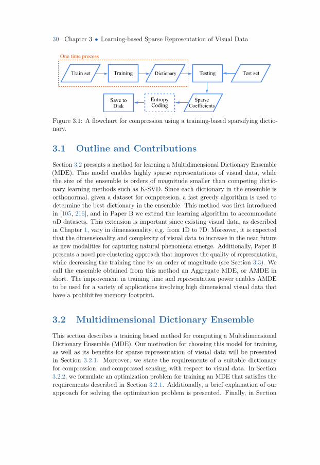
30 Chapter 3 • Learning-based Sparse Representation of Visual Data
TrainingTrain set Dictionary Testing Test set
SparseCoefficients
EntropyCoding
Save to Disk
One time process
Figure 3.1: A flowchart for compression using a training-based sparsifying dictio-nary.
3.1 Outline and ContributionsSection 3.2 presents a method for learning a Multidimensional Dictionary Ensemble(MDE). This model enables highly sparse representations of visual data, whilethe size of the ensemble is orders of magnitude smaller than competing dictio-nary learning methods such as K-SVD. Since each dictionary in the ensemble isorthonormal, given a dataset for compression, a fast greedy algorithm is used todetermine the best dictionary in the ensemble. This method was first introducedin [105, 216], and in Paper B we extend the learning algorithm to accommodatenD datasets. This extension is important since existing visual data, as describedin Chapter 1, vary in dimensionality, e.g. from 1D to 7D. Moreover, it is expectedthat the dimensionality and complexity of visual data to increase in the near futureas new modalities for capturing natural phenomena emerge. Additionally, Paper Bpresents a novel pre-clustering approach that improves the quality of representation,while decreasing the training time by an order of magnitude (see Section 3.3). Wecall the ensemble obtained from this method an Aggregate MDE, or AMDE inshort. The improvement in training time and representation power enables AMDEto be used for a variety of applications involving high dimensional visual data thathave a prohibitive memory footprint.
3.2 Multidimensional Dictionary EnsembleThis section describes a training based method for computing a MultidimensionalDictionary Ensemble (MDE). Our motivation for choosing this model for training,as well as its benefits for sparse representation of visual data will be presentedin Section 3.2.1. Moreover, we state the requirements of a suitable dictionaryfor compression, and compressed sensing, with respect to visual data. In Section3.2.2, we formulate an optimization problem for training an MDE that satisfies therequirements described in Section 3.2.1. Additionally, a brief explanation of ourapproach for solving the optimization problem is presented. Finally, in Section
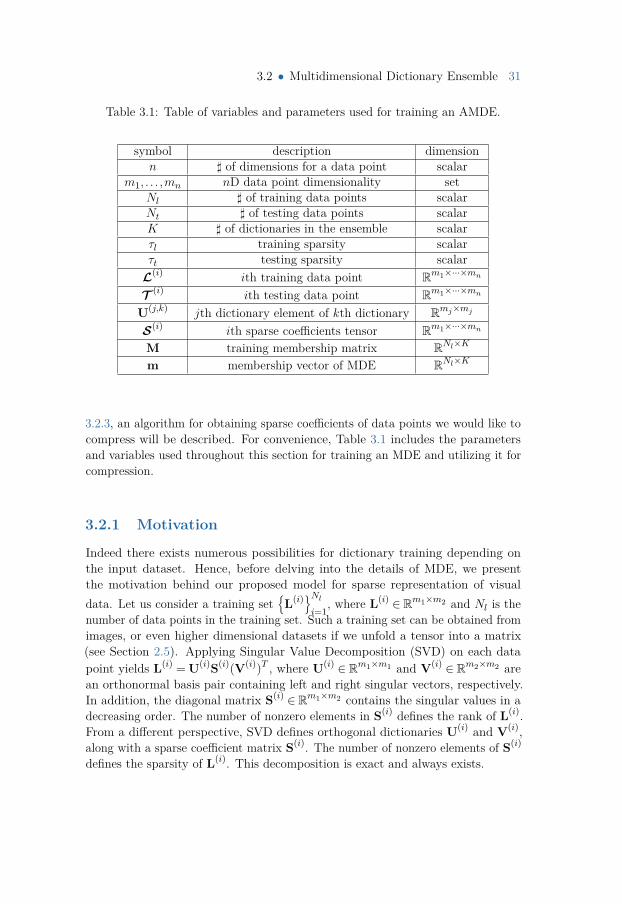
3.2 • Multidimensional Dictionary Ensemble 31
Table 3.1: Table of variables and parameters used for training an AMDE.
symbol description dimensionn ] of dimensions for a data point scalar
m1, . . . ,mn nD data point dimensionality setNl ] of training data points scalarNt ] of testing data points scalarK ] of dictionaries in the ensemble scalarτl training sparsity scalarτt testing sparsity scalarL(i) ith training data point Rm1×···×mn
T (i) ith testing data point Rm1×···×mn
U(j,k) jth dictionary element of kth dictionary Rmj×mj
S(i) ith sparse coefficients tensor Rm1×···×mn
M training membership matrix RNl×K
m membership vector of MDE RNl×K
3.2.3, an algorithm for obtaining sparse coefficients of data points we would like tocompress will be described. For convenience, Table 3.1 includes the parametersand variables used throughout this section for training an MDE and utilizing it forcompression.
3.2.1 Motivation
Indeed there exists numerous possibilities for dictionary training depending onthe input dataset. Hence, before delving into the details of MDE, we presentthe motivation behind our proposed model for sparse representation of visualdata. Let us consider a training set
L(i)Nl
i=1, where L(i) ∈ Rm1×m2 and Nl is the
number of data points in the training set. Such a training set can be obtained fromimages, or even higher dimensional datasets if we unfold a tensor into a matrix(see Section 2.5). Applying Singular Value Decomposition (SVD) on each datapoint yields L(i) = U(i)S(i)(V(i))T , where U(i) ∈ Rm1×m1 and V(i) ∈ Rm2×m2 arean orthonormal basis pair containing left and right singular vectors, respectively.In addition, the diagonal matrix S(i) ∈ Rm1×m2 contains the singular values in adecreasing order. The number of nonzero elements in S(i) defines the rank of L(i).From a different perspective, SVD defines orthogonal dictionaries U(i) and V(i),along with a sparse coefficient matrix S(i). The number of nonzero elements of S(i)
defines the sparsity of L(i). This decomposition is exact and always exists.

32 Chapter 3 • Learning-based Sparse Representation of Visual Data
For nD data points,L(i)Nl
i=1, where L(i) ∈Rm1×···×mn , a rank-revealing decompo-
sition that also produces orthogonal dictionaries does not exist. A close candidatefor this task is Higher Order SVD (HOSVD) [121] which computes the decomposi-tion
L(i) = S(i)×1 U(1,i) · · ·×nU(n,i) = S(i)n¡
j=1U(j,i), (3.1)
where U(j,i) ∈ Rmj×mj , j = 1, . . . ,n, are orthogonal dictionaries for L(i); the coeffi-cient tensor S(i) ∈ Rm1×···×mn is all-orthogonal and describes the linear relationbetween the dictionaries and the data point. Moreover, the symbol ×j definestensor-matrix multiplication along the jth mode; see Section 2.2 for more details.We can view the collection of orthonormal matrices
U(j,i)n
j=1as basis matrices
along different modes and the elements of the core tensor (S(i)) as coefficientsdescribing the linear combination of bases to form L(i).
In the case of the SVD, if a low-rank approximation is needed rather than an exactdecomposition, one can nullify elements of S(i) with the smallest absolute value.We denote the resulting matrix as S(i); hence, the approximated data point isL(i) = U(i)S(i)(V(i))T . Here, the approximation error is defined as ‖L(i)− L(i)‖F ,which is equivalent to ‖S(i)− S(i)‖F due to the invariance of the Frobenius normunder orthonormal transformations. By Eckart-Young theorem [217], the low-rankapproximation described above has the lowest error achievable with respect to anymatrix norm. This approximation method can be extended to higher dimensions viaHOSVD; i.e. by nullifying smallest elements in S(i), we obtain an approximationof L(i). However, unlike SVD, here the number of nonzero elements of S(i) doesnot indicate the rank of L(i). Tensor approximation using HOSVD has shownto produce acceptable results in practice for computer graphics and visualizationapplications [28, 34, 96, 97, 98, 218, 219].
So far we have considered the decomposition of one data point. For compression of adataset comprising of a large number of data points, two families of approaches exist.When we apply a tensor decomposition such as HOSVD on every data point in thetraining set, we obtain an ensemble of Nl orthonormal multidimensional dictionariesU(1,i),U(2,i), . . . ,U(n,i)Nl
i=1. The obtained model is highly localized, i.e. each data
point is independently represented in a unique subspace of Rm1×m2×···×mn by thecoefficients S(i). It is evident that such a model has a larger storage cost than theinput data. Therefore, compression is achieved by nullifying small elements in thecoefficient tensor S(i), see e.g. [34, 97, 98]. Note that the dictionary columns thatcorrespond to nonzero coefficients in S(i) should also be stored for each data point,which reduces the compression ratio drastically. At the other end of the spectrum,one can define a single dictionary, using e.g. Principal Component Analysis (PCA)[220], or its higher dimensional variants [221, 222]. In this model, all the data
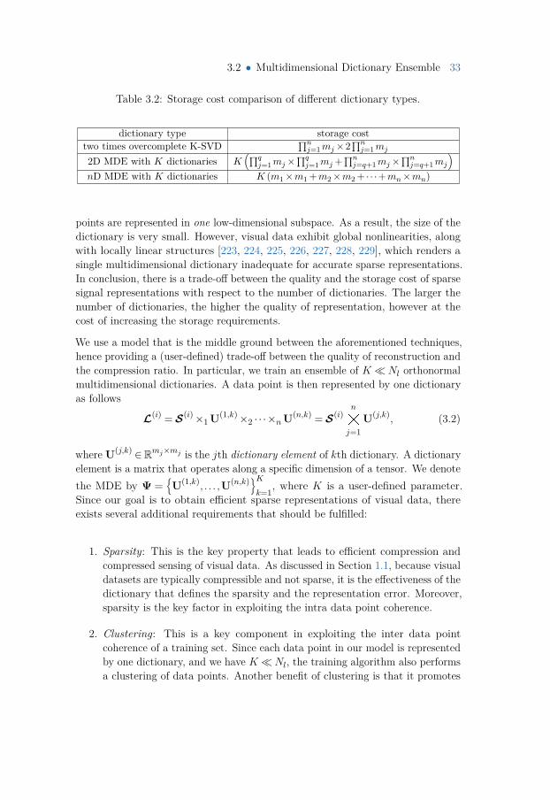
3.2 • Multidimensional Dictionary Ensemble 33
Table 3.2: Storage cost comparison of different dictionary types.
dictionary type storage costtwo times overcomplete K-SVD
∏nj=1mj×2
∏nj=1mj
2D MDE with K dictionaries K(∏q
j=1mj×∏q
j=1mj +∏n
j=q+1mj×∏n
j=q+1mj
)nD MDE with K dictionaries K (m1×m1 +m2×m2 + · · ·+mn×mn)
points are represented in one low-dimensional subspace. As a result, the size of thedictionary is very small. However, visual data exhibit global nonlinearities, alongwith locally linear structures [223, 224, 225, 226, 227, 228, 229], which renders asingle multidimensional dictionary inadequate for accurate sparse representations.In conclusion, there is a trade-off between the quality and the storage cost of sparsesignal representations with respect to the number of dictionaries. The larger thenumber of dictionaries, the higher the quality of representation, however at thecost of increasing the storage requirements.
We use a model that is the middle ground between the aforementioned techniques,hence providing a (user-defined) trade-off between the quality of reconstruction andthe compression ratio. In particular, we train an ensemble of KNl orthonormalmultidimensional dictionaries. A data point is then represented by one dictionaryas follows
L(i) = S(i)×1 U(1,k)×2 · · ·×nU(n,k) = S(i)n¡
j=1U(j,k), (3.2)
where U(j,k) ∈Rmj×mj is the jth dictionary element of kth dictionary. A dictionaryelement is a matrix that operates along a specific dimension of a tensor. We denotethe MDE by Ψ =
U(1,k), . . . ,U(n,k)K
k=1, where K is a user-defined parameter.
Since our goal is to obtain efficient sparse representations of visual data, thereexists several additional requirements that should be fulfilled:
1. Sparsity: This is the key property that leads to efficient compression andcompressed sensing of visual data. As discussed in Section 1.1, because visualdatasets are typically compressible and not sparse, it is the effectiveness of thedictionary that defines the sparsity and the representation error. Moreover,sparsity is the key factor in exploiting the intra data point coherence.
2. Clustering: This is a key component in exploiting the inter data pointcoherence of a training set. Since each data point in our model is representedby one dictionary, and we have KNl, the training algorithm also performsa clustering of data points. Another benefit of clustering is that it promotes
34 Chapter 3 • Learning-based Sparse Representation of Visual Data
the sparsity in the representation since it is unlikely that the entire trainingset is sparse in one dictionary.
3. Representativeness: In practice, we would like to perform the training once,and use the ensemble on a test set. The test set is a collection of datapoints that we would like to compress, or perform compressed sensing on.Since the test set is typically much larger than the training set, the trainedensemble should be efficient enough to enable sparse representation of theunobserved data points in the test set. This property is not possessed bytensor decomposition based methods such as [34, 96, 97, 98, 230].
4. Arbitrary dimensionality: Since we consider visual data, which are verydiverse in terms of dimensionality, the dictionary ensemble should enablesparse representations regardless of the data dimensionality.
5. Small dictionary size: Since the MDE is trained from a set of examples, itneeds to be stored for compression and compressed sensing. This is in contrastto analytical dictionaries where the dictionary is evaluated during encoding ordecoding. Therefore, the size of the MDE is important for compression. A keycomponent in reducing the size of the MDE is multidimensionality. Tensordecomposition and 1D dictionaries have very large memory footprints, whichmakes the transmission of the dictionary to the decoder very challenging[34, 162, 230]. See Table 3.2 for a storage cost comparison of differentdictionary types (and see Section 4.3 for numerical comparisons).
6. Fast local reconstruction: For real time rendering of e.g. light field and lightfield videos, efficient local reconstruction of the compressed data is essential.This property is achieved by the orthogonality of dictionaries (examples ofthe local real time reconstruction of visual data will be given in Chapter 4).Moreover, since the ensemble is small, the reconstruction process can be fullyimplemented on the GPU.
In the following section, we formulate the problem of training an MDE that fulfillsthe requirements stated above.
3.2.2 Training
Given the requirements stated in Section 3.2.1, and inspired by [105, 216], weformulate the problem of training an MDE that enables the sparse representation
3.2 • Multidimensional Dictionary Ensemble 35
of visual data as follows
minU(j,k)
,S(i,k),M
Nl∑i=1
K∑k=1
Mi,k
∥∥∥∥∥∥L(i)−S(i,k)n¡
j=1U(j,k)
∥∥∥∥∥∥2
F
, subject to (3.3a)
(U(j,k))T U(j,k) = I, ∀k = 1, . . . ,K, ∀j = 1, . . . ,n, (3.3b)∥∥∥S(i,k)
∥∥∥0≤ τl, (3.3c)
K∑k=1
Mi,k = 1, ∀i= 1, . . . ,Nl. (3.3d)
The objective function, i.e. (3.3a), measures the representation error over all datapoints and dictionaries. Because each data point is represented by one dictionary,we need a clustering matrix to enforce this structure on the objective function.We call the clustering matrix M ∈ RNl×K a membership matrix, a binary matrixassociating each data point L(i) to its corresponding dictionary
U(1,k), . . . ,U(n,k)
in the MDE. Each row in M has only one non-zero component to guarantee that adata point uses one dictionary; this is enforced by the constraint in (3.3d). Thesparsity of the coefficient tensor S(i,k) is enforced by the constraint in (3.3c), whereτl is a user-defined parameter for sparsity. Moreover, equation (3.3b) puts anorthonormality constraint on the dictionaries. We denote the process of trainingan MDE by the following function
U(1,k), . . . ,U(n,k)K
k=1= Train
(L(i)Nl
i=1,K,τl
). (3.4)
Note that although the training stage computes U(j,k), S(i,k), and M, we only needthe MDE, i.e. Ψ =
U(1,k), . . . ,U(n,k)K
k=1. This is because the test set is different
from the training set, and hence we need a new set of sparse coefficients and amembership matrix. Moreover, since we have three sets of unknowns in (3.3), weiteratively update each variable while fixing the others. The update rules are asfollows
S(i,k) = L(i)×1(U(1,k))T · · ·×n (U(n,k))T , (3.5)
U(j,k) = Z(j,k)((
Z(j,k))T Z(j,k))−1/2
, (3.6)
where
Z(j,k) =Nl∑i=1
Mi,kL(i)(j)
(U(n,k)⊗·· ·⊗U(j+1,k)⊗
U(j−1,k)⊗·· ·⊗U(1,k))(S(i,k)(j)
)T. (3.7)
36 Chapter 3 • Learning-based Sparse Representation of Visual Data
Moreover,
Mi,k = K∑b=1
eβ(δik−δib)−1
, (3.8)
whereδik =
∥∥∥L(i)−S(i,k)×1 U(1,k) · · ·×nU(n,k)∥∥∥2
F. (3.9)
The temperature parameter, β, in equation (3.8) is initialized with a small value.For a fixed value of β, the sequential updates are repeated until the convergence ofΨ. Then, the temperature parameter is increased and the same update procedureis repeated. The algorithm converges when M is binary. The supplementarymaterials of Paper B contains a pseudo code describing the training process inmore details. The derivation of the update rules above is a fairly straightforwardextension of the methods used in [105] from 2D data points to general nD datapoints. Using the method of Lagrange multipliers, we can rewrite (3.3) as
Nl∑i=1
K∑k=1
Mi,k
∥∥∥∥∥∥L(i)−S(i,k)n¡
j=1U(j,k)
∥∥∥∥∥∥2
F
+ 1β
Nl∑i=1
K∑k=1
Mi,k log(Mi,k) +Nl∑i=1
µi
K∑k=1
Mi,k−1
+n∑j=1
K∑k=1
Tr(
Λ(j,k)((
U(j,k))T U(j,k)− I))
, (3.10)
where µi and Λ(j,k) are Lagrange multipliers (note that Λ(j,k) are symmetricmatrices). The term Mi,k log(Mi,k) is an entropy barrier function [231] thatensures the positivity of Mi,k. The update rule for Mi,k in (3.8) is independentof the data dimensionality as long as an error function associating a data pointto a dictionary is defined (e.g. equation (3.9)). See [232] for the derivation of(3.8). Moreover, the update rule for S(i,k) in (3.5), followed by the nullification ofthe small elements of S(i,k), is a trivial extension of Theorem 2 in [105]. For theupdate rule of U(j,k), k ∈ 1, . . . ,K, j ∈ 1, . . . ,n, we first gather and rewrite theterms in (3.10) that are dependent on U(j,k) (i.e. one dictionary element). Using(2.9), and due to the invariance of the Frobenius norm to tensor unfolding, we canrewrite (3.10) as
∑i,k
Mi,kTr(GTG
)+
K∑k=1
Tr(
Λ(j,k)((
U(j,k))T U(j,k)− I))
+C, (3.11)
where C contains the terms that are independent of U(j,k), and
G = L(i)(j)−U(j,k)S(i,k)
(j)
⊗α=n,...,1\j
U(α,k)T . (3.12)
3.2 • Multidimensional Dictionary Ensemble 37
For notational brevity, define
U =∆⊗
α=n,...,1\jU(α,k). (3.13)
Then, expanding the term Tr(GTG
)in (3.11), and using the properties of the
matrix trace, we obtain
∑i,k
Mi,k
[Tr((
L(i)(j)
)TL(i)
(j)
)−2Tr
((L(i)
(j)
)TU(j,k)S(i,k)
(j) UT
)
+Tr(
U(S(i,k)
(j)
)T (U(j,k))T U(j,k)S(i,k)
(j) UT
)]+
K∑k=1
Tr(
Λ(j,k)((
U(j,k))T U(j,k)− I))
+C. (3.14)
Setting the derivatives with respect to U(j,k) and Λ(j,k) to zero leads to the followingsystem of equations (see [233] for a comprehensive review of matrix derivativerules)
2∑i
Mi,k
(−L(i)
(j) +U(j,k)S(i,k)(j) UT
)U(S(i,k)
(j)
)T+U(j,k)
((Λ(j,k))T + Λ(j,k)
)= 0,(
U(j,k))T U(j,k)− I = 0(3.15)
A similar optimization problem was considered in [216], where the authors proposea closed form solution for obtaining a basis given a collection of one-dimensionaldata points and subject to an orthonormality constraint. According to [216], thesolution of (3.15) can be calculated as U(j,k) = LRT , where L and R are left andright singular vectors of Z(j,k), defined in (3.7).
3.2.3 Testing
LetT (i)Nt
i=1denote a test set containing Nt data points, where the test set is a
collection of data points that we would like to compress. The process of obtaininga set of sparse coefficient tensors corresponding to the data points in the test setis called testing. In addition to the sparse coefficient tensors, the testing processshould also determine the most suitable dictionary in the MDE for each data point.Thanks to the orthonormalilty of the dictionaries, the testing process is simple.In Algorithm 2, we outline a greedy algorithm based on [105] that achieves thisgoal. The algorithm takes as input a data point and an MDE, and outputs a sparsecoefficient tensor, as well as an integer holding the index of a dictionary in theMDE that leads to the best sparse representation of the data point. Therefore
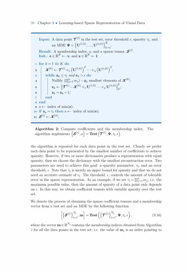
38 Chapter 3 • Learning-based Sparse Representation of Visual Data
Input: A data point T (i) in the test set, error threshold ε, sparsity τt, andan MDE Ψ =
U(1,k), . . . ,U(n,k)K
k=1.
Result: A membership index, a, and a sparse tensor, S(i).Init.: e ∈ RK ←∞ and z ∈ RK ← 1
1 for k = 1 to K do2 X (k)← T (i)×1
(U(1,k))T · · ·×n (U(n,k))T ;
3 while zk ≤ τt and ek > ε do4 Nullify (∏nj=1mj)−zk smallest elements of X (k);5 ek←
∥∥∥T (i)−X (k)×1 U(1,k) · · ·×nU(n,k)∥∥∥2
F;
6 zk = zk + 1;7 end8 end9 a← index of min(z);
10 if za = τt then a← index of min(e);11 S(i)←X (a);
Algorithm 2: Compute coefficients and the membership index. Thealgorithm implements
S(i),a
= Test
(T (i),Ψ, τt, ε
).
the algorithm is repeated for each data point in the test set. Clearly we prefereach data point to be represented by the smallest number of coefficients to achievesparsity. However, if two or more dictionaries produce a representation with equalsparsity, then we choose the dictionary with the smallest reconstruction error. Twoparameters are used to achieve this goal: a sparsity parameter, τt, and an errorthreshold, ε. Note that τt is merely an upper bound for sparsity and that we do notneed an accurate estimate of τt. The threshold, ε, controls the amount of tolerableerror in the sparse representation. As an example, if we set τt =∏n
j=1mj , i.e. themaximum possible value, then the amount of sparsity of a data point only dependson ε. In this way, we obtain coefficient tensors with variable sparsity over the testset.
We denote the process of obtaining the sparse coefficient tensors and a membershipvector from a test set and an MDE by the following function[
S(i)Nti=1
,m]
= Test(
T (i)Nti=1
,Ψ, τt, ε), (3.16)
where the vector m∈RNt contains the membership indices obtained from Algorithm2 for all the data points in the test set; i.e. the value of mi is an index pointing to
3.3 • Pre-clustering 39
a dictionary in the MDE that is used for the data point T (i). If the dictionaries arenot orthonormal, then one has to solve an `0 problem using e.g. OMP, as discussedin Section 2.4. The computational complexity of Algorithm 2 is significantly lowerthan OMP, which is among the fastest `0 solvers. The speedup achieved usingan MDE facilitates the compression of large-scale datasets. We will discuss theexamples of compressing large-scale visual data in Chapter 4.
3.3 Pre-clusteringIn this section, we discuss an algorithm for improving the performance of MDE withregards to the computational complexity of the training and the representativenessof the ensemble. We achieve this by performing a pre-clustering of the training set,followed by training an MDE for each pre-cluster. This approach assists the MDEtraining in finding a more suitable set of dictionaries for sparse representation. Ourmotivation for pre-clustering is described in more details in Section 3.3.1. Moreover,the pre-clustering algorithm will be presented in Section 3.3.2.
3.3.1 MotivationThe training algorithm discussed in Section 3.2 is a powerful tool for sparserepresentation of visual data. In Section 1.1 we discussed how sometimes there aredata points that do not admit a sparse representation in a dictionary (see Fig. 1.3).Our solution was to add a new atom (in the case of an overcomplete dictionary),or to add a new orthogonal dictionary (for an orthogonal dictionary ensemble).Considering complex datasets such as light fields, it is not unlikely that a trainedMDE with a limited number of dictionaries would fail in the sparse representationof the entire domain of light fields. Given that a test set containing all the possiblelight fields is practically infinite, we can only improve our model to alleviate theproblem of representation error. One approach is to train an ensemble with a largernumber of dictionaries. However, with large-scale datasets, training a large numberof dictionaries quickly becomes intractable. In Paper B, we choose a differentapproach by applying pre-clustering to the training set, followed by learning anensemble for each pre-cluster. We use the term “pre-clustering” since learning anMDE includes a clustering of the training set using the membership matrix M.
An important factor in any clustering algorithm is the choice of a metric forcomputing pairwise distances between data points. For instance, K-Means [16] usesan `2 distance metric between points and have been used in computer graphics andvisualization for different applications [228, 234, 235, 236, 237]. K-Means is alsoan important component in other clustering algorithms, e.g. spectral clustering[238, 239]. In Section 3.2 we described the requirements for choosing a dictionaryin an ensemble. In particular, the metric is defined to be based on the sparsity
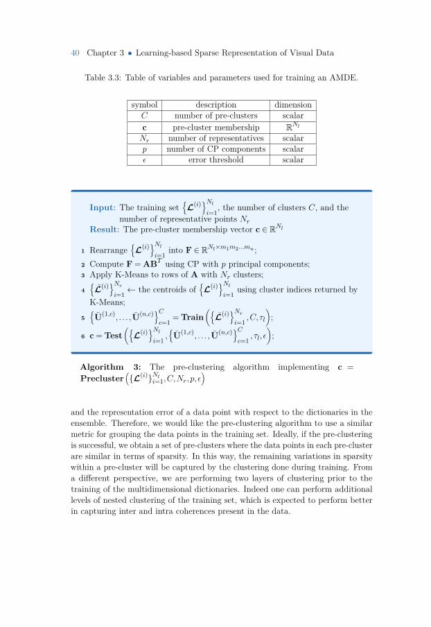
40 Chapter 3 • Learning-based Sparse Representation of Visual Data
Table 3.3: Table of variables and parameters used for training an AMDE.
symbol description dimensionC number of pre-clusters scalarc pre-cluster membership RNlNr number of representatives scalarp number of CP components scalarε error threshold scalar
Input: The training setL(i)Nl
i=1, the number of clusters C, and the
number of representative points NrResult: The pre-cluster membership vector c ∈ RNl
1 RearrangeL(i)Nl
i=1into F ∈ RNl×m1m2...mn ;
2 Compute F = ABT using CP with p principal components;3 Apply K-Means to rows of A with Nr clusters;4L(i)Nr
i=1← the centroids of
L(i)Nl
i=1using cluster indices returned by
K-Means;5U(1,c), . . . ,U(n,c)C
c=1= Train
(L(i)Nr
i=1,C,τl
);
6 c = Test(
L(i)Nli=1
,U(1,c), . . . ,U(n,c)C
c=1, τl, ε
);
Algorithm 3: The pre-clustering algorithm implementing c =Precluster
(L(i)Nli=1,C,Nr,p, ε
)
and the representation error of a data point with respect to the dictionaries in theensemble. Therefore, we would like the pre-clustering algorithm to use a similarmetric for grouping the data points in the training set. Ideally, if the pre-clusteringis successful, we obtain a set of pre-clusters where the data points in each pre-clusterare similar in terms of sparsity. In this way, the remaining variations in sparsitywithin a pre-cluster will be captured by the clustering done during training. Froma different perspective, we are performing two layers of clustering prior to thetraining of the multidimensional dictionaries. Indeed one can perform additionallevels of nested clustering of the training set, which is expected to perform betterin capturing inter and intra coherences present in the data.
3.3 • Pre-clustering 41
3.3.2 Aggregate Multidimensional Dictionary EnsemblePaper B presents a pre-clustering algorithm that groups the data points based ontheir sparsity and representation error. In addition, the pre-clustering is designedsuch that the effect of noise and outliers in the data is reduced. For convenience,Table 3.3 includes all the parameters used for the training of a pre-clustered MDE.Algorithm 3 presents a pseudo code for the pre-clustering method, and in whatfollows we provide a brief description as well as our motivation for each of the stepsinvolved.
First, we reduce the dimensionality of the data points in the training set. Fornotational brevity, define m=∏n
j=1mj . The decomposition F = ABT is performed,where F ∈ RNl×m contains vectorized data points as rows, A ∈ RNl×p containscoefficients in each row, and B∈Rm1m2...mn×p has a set of basis vectors as columns.When pm, we achieve a dimensionality reduction of the data points. In otherwords, the rows of A are now relatively low dimensional vectors that approximatethe large multidimensional data points of the training set. A popular choice forperforming this decomposition is Principal Component Analysis (PCA). However,PCA is known to be notoriously sensitive to outliers and noise [240]. Unfortunately,visual datasets are prone to noise and outliers due to the imperfections in thesensing process used to capture the data. Instead of PCA, we propose to useCoherence Pursuit (CP) [241], a Robust-PCA algorithm [211, 242] that is simpleand fast, with strong theoretical guarantees.
Next, we apply K-Means on the rows of A with Nr clusters. Our goal here is toobtain a subset of the training set that is representative of the entire set. Theuser-defined parameter Nr controls the number of representative data points. Usingthe obtained cluster indices from K-Means, the centroids of
L(i)Nl
i=1are calculated.
In other words, we calculate the mean of data points that are inside a K-Meanscluster. One can also choose a data point from a K-Means cluster at random. Wecall these centroids the representative set, denoted
L(i)Nr
i=1. The representative
set is then used to train an MDE with C dictionaries, where C is the numberof user-defined pre-clusters. Finally, the trained MDE, together with the entiretraining set, are used to produce a membership vector c ∈ RNl using Algorithm 2,which associates each data point in the training set to a pre-cluster. We use thefollowing function to denote the pre-clustering of a training set
c = Precluster(
L(i)Nli=1
,C,Nr,p, ε), (3.17)
A thorough numerical analysis of the user-defined parameters (see Table 3.1)is presented in the supplementary materials of Paper B. The most importantparameters are C and K. In practice, we would like to increase C and K as longas the computational cost of the training is acceptable. The values of these two
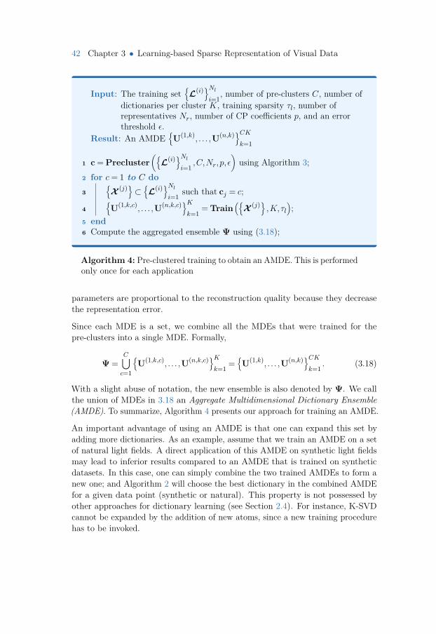
42 Chapter 3 • Learning-based Sparse Representation of Visual Data
Input: The training setL(i)Nl
i=1, number of pre-clusters C, number of
dictionaries per cluster K, training sparsity τl, number ofrepresentatives Nr, number of CP coefficients p, and an errorthreshold ε.
Result: An AMDEU(1,k), . . . ,U(n,k)CK
k=1
1 c = Precluster(
L(i)Nli=1
,C,Nr,p, ε)using Algorithm 3;
2 for c= 1 to C do3
X (j)⊂ L(i)Nl
i=1such that cj = c;
4U(1,k,c), . . . ,U(n,k,c)K
k=1= Train
(X (j) ,K,τl);
5 end6 Compute the aggregated ensemble Ψ using (3.18);
Algorithm 4: Pre-clustered training to obtain an AMDE. This is performedonly once for each application
parameters are proportional to the reconstruction quality because they decreasethe representation error.
Since each MDE is a set, we combine all the MDEs that were trained for thepre-clusters into a single MDE. Formally,
Ψ =C⋃c=1
U(1,k,c), . . . ,U(n,k,c)K
k=1=U(1,k), . . . ,U(n,k)CK
k=1. (3.18)
With a slight abuse of notation, the new ensemble is also denoted by Ψ. We callthe union of MDEs in 3.18 an Aggregate Multidimensional Dictionary Ensemble(AMDE). To summarize, Algorithm 4 presents our approach for training an AMDE.
An important advantage of using an AMDE is that one can expand this set byadding more dictionaries. As an example, assume that we train an AMDE on a setof natural light fields. A direct application of this AMDE on synthetic light fieldsmay lead to inferior results compared to an AMDE that is trained on syntheticdatasets. In this case, one can simply combine the two trained AMDEs to form anew one; and Algorithm 2 will choose the best dictionary in the combined AMDEfor a given data point (synthetic or natural). This property is not possessed byother approaches for dictionary learning (see Section 2.4). For instance, K-SVDcannot be expanded by the addition of new atoms, since a new training procedurehas to be invoked.
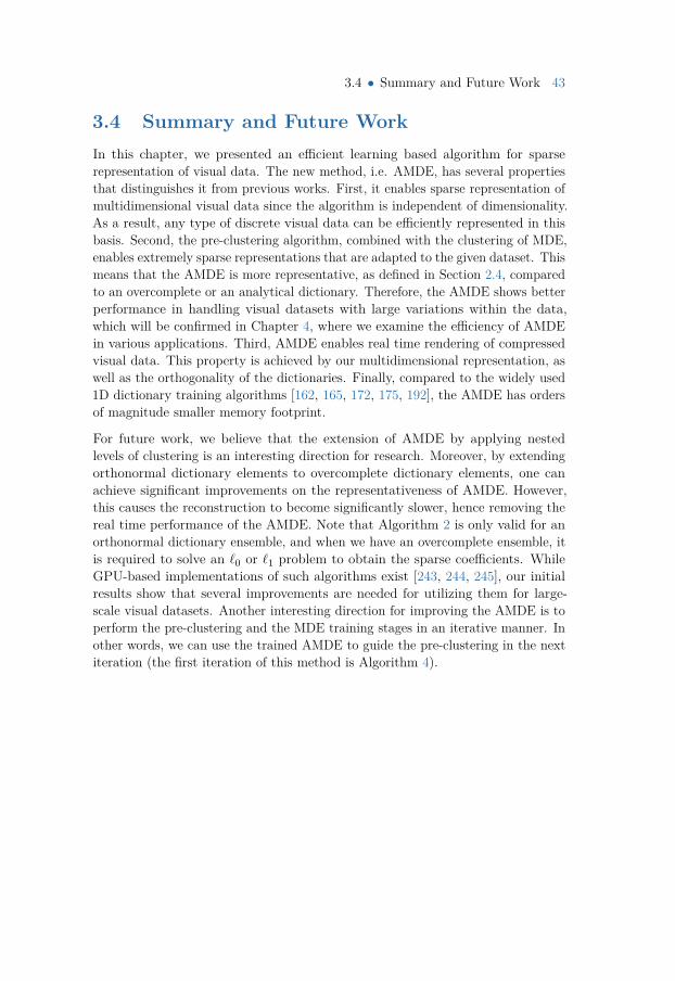
3.4 • Summary and Future Work 43
3.4 Summary and Future WorkIn this chapter, we presented an efficient learning based algorithm for sparserepresentation of visual data. The new method, i.e. AMDE, has several propertiesthat distinguishes it from previous works. First, it enables sparse representation ofmultidimensional visual data since the algorithm is independent of dimensionality.As a result, any type of discrete visual data can be efficiently represented in thisbasis. Second, the pre-clustering algorithm, combined with the clustering of MDE,enables extremely sparse representations that are adapted to the given dataset. Thismeans that the AMDE is more representative, as defined in Section 2.4, comparedto an overcomplete or an analytical dictionary. Therefore, the AMDE shows betterperformance in handling visual datasets with large variations within the data,which will be confirmed in Chapter 4, where we examine the efficiency of AMDEin various applications. Third, AMDE enables real time rendering of compressedvisual data. This property is achieved by our multidimensional representation, aswell as the orthogonality of the dictionaries. Finally, compared to the widely used1D dictionary training algorithms [162, 165, 172, 175, 192], the AMDE has ordersof magnitude smaller memory footprint.
For future work, we believe that the extension of AMDE by applying nestedlevels of clustering is an interesting direction for research. Moreover, by extendingorthonormal dictionary elements to overcomplete dictionary elements, one canachieve significant improvements on the representativeness of AMDE. However,this causes the reconstruction to become significantly slower, hence removing thereal time performance of the AMDE. Note that Algorithm 2 is only valid for anorthonormal dictionary ensemble, and when we have an overcomplete ensemble, itis required to solve an `0 or `1 problem to obtain the sparse coefficients. WhileGPU-based implementations of such algorithms exist [243, 244, 245], our initialresults show that several improvements are needed for utilizing them for large-scale visual datasets. Another interesting direction for improving the AMDE is toperform the pre-clustering and the MDE training stages in an iterative manner. Inother words, we can use the trained AMDE to guide the pre-clustering in the nextiteration (the first iteration of this method is Algorithm 4).

Ch
ap
te
r
4Compression of Visual Data
Compression has been utilized in computer graphics in several applications [97,98, 246, 247, 248]. However, learning based methods for the sparse representationof visual data have received little attention. Hence, one of the main goals of thisthesis is to describe and analyze methods for efficient sparse representations ofvisual data that enable high compression ratios with minimal degradation in imagequality, as well as real time rendering of the compressed data. Utilizing the MDEand the AMDE, introduced in Chapter 3, in this chapter we will present threeapplications for the efficient compression of visual data using sparse representations.While a full compression framework may entail several other steps, such as entropycoding, we only focus on finding suitable transformations of the visual data usingthe learning based dictionary ensembles. Indeed any entropy coding algorithm canbe applied on top of the methods we introduce in this chapter.
4.1 Outline and ContributionsIn Section 4.2, we utilize MDE and K-Means to compress surface light fields forreal time photorealistic rendering of highly complex static scenes. The methodwas presented in Paper A and the results show significant improvements overclustered principal component analysis [228], spherical harmonics [44], and K-SVD.In Section 4.3, we use the AMDE for the compression of light field and light fieldvideo datasets. The proposed method outperforms well-established analytical basisfunctions, as well as training based dictionaries. More importantly, we show thatthe AMDE enables real time GPU-based rendering of high resolution light field
46 Chapter 4 • Compression of Visual Data
videos that consume hundreds of gigabytes of storage. More detailed analysisof these results can be found in Paper B. Finally, in Section 4.4, we utilize theAMDE for the compression of datasets obtained from a device for appearancecapture of relatively large scenes. A rotating arc containing several high resolutioncameras covering the full hemisphere above the scene captures more than 300gigabytes of data in a few seconds. After the compression of the data using theAMDE, real time exploration of the scene using e.g. virtual reality goggles is madepossible. While the results are not published yet, they are included in this thesisto show the effectiveness of the AMDE in various applications. We would like toemphasize that since the AMDE can be trained on any discrete visual datasetwith an arbitrary dimensionality, the results presented here are merely examples ofpossible applications for the proposed method.
4.2 Precomputed Photorealistic RenderingThis section will present a method for real time photorealistic rendering of highlycomplex scenes by pre-computing the Surface Light Field (SLF) of a scene. Giventhe large amount of data generated by SLFs, we apply a variant of MDE tocompress this data. Moreover, we demonstrate high-quality real time rendering ofthe compressed SLF datasets using the GPU. We start by stating our motivationfor choosing precomputed photorealistic rendering over approximate real timeray tracing methods in Section 4.2.1. An overview of the method is presented inSection 4.2.2. Moreover, various stages of the algorithm are described in sections4.2.3–4.2.5, followed by the results in Section 4.2.6.
4.2.1 Background and MotivationPhotorealistic rendering is one of the key challenges in computer graphics. Decadesof research has culminated in numerous methods for achieving photorealism inrendered images. While a significant progress has been made to this date, ourdefinition of “photorealism” is also evolving. Moreover, as new techniques for ren-dering emerge, the amount of required computational power increases dramatically.Inadequate computing power has been a common trend in the field since the dawn ofphotorealistic rendering techniques [249, 250], a trend that is expected to continuein the future as our expectations of photorealism evolves. Today, a photorealisticrendering of a scene can take minutes to hours, or even days on multi-processorand multi-computer architectures. As a result, real time photorealistic renderingon a consumer level personal computer is a very challenging task. Several methodshave been proposed in this direction, mostly relying on approximation techniquesfor ray tracing that utilize modern GPUs. However, existing methods only focuson certain components of the photorealistic rendering, or simulate a certain natural
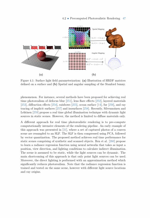
4.2 • Precomputed Photorealistic Rendering 47
(a)
−1
−0.5
0
0.5
1
−1
−0.8
−0.6
−0.4
−0.2
0
0.2
0.4
0.6
0.8
1
0
0.2
0.4
0.6
0.8
1
X
Y
Z
Spatial Mapping
Angular Mappingξ1 ∈ [0, 1]
ξ2 ∈ [0, 1]
u ∈ [0, 1]
v ∈ [0, 1] (u, v) −→ (x, y, z)
(u, v)←− (x, y, z)
[0, 1]2 −→ (r, φ) −→ ~d
[0, 1]2 ←− (r, φ)←− ~d
(b)
Figure 4.1: Surface light field parameterization: (a) Illustration of HRDF matricesdefined on a surface and (b) Spatial and angular sampling of the Stanford bunny.
phenomenon. For instance, several methods have been proposed for achieving realtime photorealism of defocus blur [251], lens flare effects [252], layered materials[253], diffraction effects [254], rainbows [255], ocean surface [14], fur [256], and raytracing of implicit surfaces [257] and isosurfaces [258]. Recently, Silvennoinen andLehtinen [259] propose a real time global illumination technique with dynamic lightsources in static scenes. However, the method is limited to diffuse materials only.
A different approach for real time photorealistic rendering is to pre-computecomputationally intensive elements of the rendering pipeline. An early example ofthis approach was presented in [31], where a set of captured photos of a convexscene are resampled to an SLF. The SLF is then compressed using PCA, followedby vector quantization. The proposed method achieves real time performance forstatic scenes comprising of synthetic and scanned objects. Ren et al. [260] proposeto learn a radiance regression function using neural networks that takes as input aposition, view direction, and lighting conditions to calculate indirect illumination.The scene is assumed to be static, while the light sources can be dynamic. Themain shortcoming of this approach is that only point light sources can be used.Moreover, the direct lighting is performed with an approximation method whichsignificantly reduces photorealism. Note that the radiance regression function istrained and tested on the same scene, however with different light source locationsand ray origins.
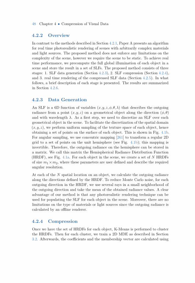
48 Chapter 4 • Compression of Visual Data
4.2.2 OverviewIn contrast to the methods described in Section 4.2.1, Paper A presents an algorithmfor real time photorealistic rendering of scenes with arbitrarily complex materialsand light sources. The proposed method does not enforce any limitations on thecomplexity of the scene, however we require the scene to be static. To achieve realtime performance, we precompute the full global illumination of each object in ascene and store the result in a set of SLFs. The proposed method consists of threestages: 1. SLF data generation (Section 4.2.3), 2. SLF compression (Section 4.2.4),and 3. real time rendering of the compressed SLF data (Section 4.2.5). In whatfollows, a brief description of each stage is presented. The results are summarizedin Section 4.2.6.
4.2.3 Data GenerationAn SLF is a 6D function of variables (x,y,z,φ,θ,λ) that describes the outgoingradiance from a point (x,y,z) on a geometrical object along the direction (φ,θ)and with wavelength λ. As a first step, we need to discretize an SLF over eachgeometrical object in the scene. To facilitate the discretization of the spatial domain(x,y,z), we perform uniform sampling of the texture space of each object, henceobtaining a set of points on the surface of each object. This is shown in Fig. 4.1b.For angular sampling, we use concentric mapping [261] to transform a regular 2Dgrid to a set of points on the unit hemisphere (see Fig. 4.1b); this mapping isinvertible. Therefore, the outgoing radiance on the hemisphere can be stored ina matrix. We call this matrix the Hemispherical Radiance Distribution Function(HRDF), see Fig. 4.1a. For each object in the scene, we create a set of N HRDFsof size m1×m2, where these parameters are user defined and describe the requiredangular resolution.
At each of the N spatial location on an object, we calculate the outgoing radiancealong the directions defined by the HRDF. To reduce Monte Carlo noise, for eachoutgoing direction in the HRDF, we use several rays in a small neighborhood ofthe outgoing direction and take the mean of the obtained radiance values. A clearadvantage of our method is that any photorealistic rendering technique can beused for populating the SLF for each object in the scene. Moreover, there are nolimitations on the type of materials or light sources since the outgoing radiance iscalculated by an offline renderer.
4.2.4 CompressionOnce we have the set of HRDFs for each object, K-Means is performed to clusterthe HRDFs. Then for each cluster, we train a 2D MDE as described in Section3.2. Afterwards, the coefficients and the membership vector are calculated using
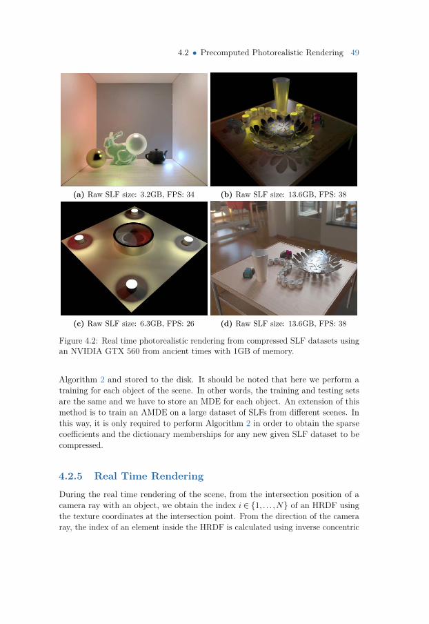
4.2 • Precomputed Photorealistic Rendering 49
(a) Raw SLF size: 3.2GB, FPS: 34 (b) Raw SLF size: 13.6GB, FPS: 38
(c) Raw SLF size: 6.3GB, FPS: 26 (d) Raw SLF size: 13.6GB, FPS: 38
Figure 4.2: Real time photorealistic rendering from compressed SLF datasets usingan NVIDIA GTX 560 from ancient times with 1GB of memory.
Algorithm 2 and stored to the disk. It should be noted that here we perform atraining for each object of the scene. In other words, the training and testing setsare the same and we have to store an MDE for each object. An extension of thismethod is to train an AMDE on a large dataset of SLFs from different scenes. Inthis way, it is only required to perform Algorithm 2 in order to obtain the sparsecoefficients and the dictionary memberships for any new given SLF dataset to becompressed.
4.2.5 Real Time Rendering
During the real time rendering of the scene, from the intersection position of acamera ray with an object, we obtain the index i ∈ 1, . . . ,N of an HRDF usingthe texture coordinates at the intersection point. From the direction of the cameraray, the index of an element inside the HRDF is calculated using inverse concentric
50 Chapter 4 • Compression of Visual Data
(a) Reference rendering
(b) MDE∗
(c) CPCA
(d) MDE∗ false color
(e) CPCA false color
Figure 4.3: Insets from Fig. 4.2, comparing a reference rendering, MDE∗, andCPCA. The reference rendering uses raw SLF data from an offline renderer.
mapping. Indeed, for each image pixel to be rendered, we only need a single valuefrom an HRDF that corresponds to the view direction. Obtaining this value isstraightforward due to the orthonormality of the dictionaries. Let H(i)
x1,x2 be anelement at location (x1,x2) of the ith HRDF, then
4.3 • Light Field and Light Field Video 51
H(i)x1,x2 =
zi∑z=1
U(1,mi)x1,l
z1
S(i)lz1 ,lz2U(2,mi)x2,l
z2, (4.1)
where m is the membership vector, zi is the number of nonzero elements in S(i),and (lz1, lz2) defines the location of nonzero values in S(i).
4.2.6 ResultsTo evaluate the method, we construct three scenes as shown in Fig. 4.2. For datageneration, we used the PBRT renderer [15] because it is an open-source softwareand we could embed our SLF data generator. The geometry, materials, and lightsources were designed to challenge the compression method rather than producingvery realistic renderings. For instance, we use multiple points light sources andhighly specular measured materials (e.g. gold and silver) to produce extremelyhigh frequency variations inside each HRDF. Indeed this is very challenging for acompression method. The Cornell box in Fig. 4.2a contains an area light sourceon the ceiling and three point light sources. The scene in Fig. 4.2b contains 10point light sources, and Fig. 4.2d shows our results for the same scene under imagebased lighting. Figure 4.2c has 6 point light sources and the gold ring has a perfectspecular component to cast caustics on the plane. In Fig. 4.3 we include insetsfrom these scenes and compare the results with CPCA compression, and the rawSLF data. Our method significantly outperforms CPCA in retaining the details ofthe SLF data. For very high frequency materials, e.g. the gold ring in Fig. 4.2c,CPCA fails to capture the details.
4.3 Light Field and Light Field VideoIn Paper B, we use the AMDE for the compression of light fields and light fieldvideos. For light fields, the Stanford Lego Gantry dataset1 is used, which consists oftwelve light fields with angular resolution of 17×17 and a variable spatial resolution(typically 1024×1024). We used 8×8 central views of the light fields and constructdata points with dimensionality m1 = 5, m2 = 5, m3 = 8, m4 = 8, and m5 = 3; i.e.we create 5×5 patches over each light field view image. The following parameterswere used to train an AMDE: C = 16, K = 8, τl = 20, p = 128, and Nr = 4000.Therefore, the dictionaries in the AMDE have the dimensionalityU(1,k) ∈ R5×5,U(2,k) ∈ R5×5,U(3,k) ∈ R8×8,
U(4,k) ∈ R8×8,U(5,k) ∈ R3×3128
k=1. (4.2)
1 http://lightfield.stanford.edu
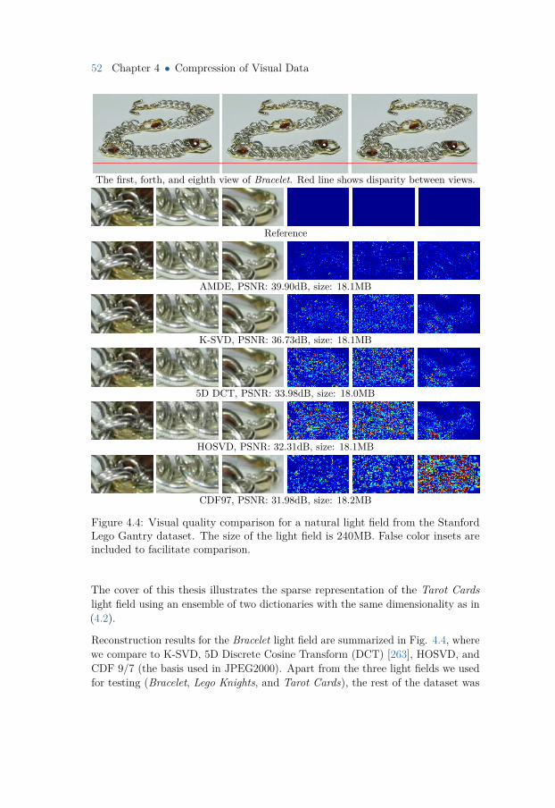
52 Chapter 4 • Compression of Visual Data
The first, forth, and eighth view of Bracelet. Red line shows disparity between views.
Reference
AMDE, PSNR: 39.90dB, size: 18.1MB
K-SVD, PSNR: 36.73dB, size: 18.1MB
5D DCT, PSNR: 33.98dB, size: 18.0MB
HOSVD, PSNR: 32.31dB, size: 18.1MB
CDF97, PSNR: 31.98dB, size: 18.2MB
Figure 4.4: Visual quality comparison for a natural light field from the StanfordLego Gantry dataset. The size of the light field is 240MB. False color insets areincluded to facilitate comparison.
The cover of this thesis illustrates the sparse representation of the Tarot Cardslight field using an ensemble of two dictionaries with the same dimensionality as in(4.2).
Reconstruction results for the Bracelet light field are summarized in Fig. 4.4, wherewe compare to K-SVD, 5D Discrete Cosine Transform (DCT) [263], HOSVD, andCDF 9/7 (the basis used in JPEG2000). Apart from the three light fields we usedfor testing (Bracelet, Lego Knights, and Tarot Cards), the rest of the dataset was
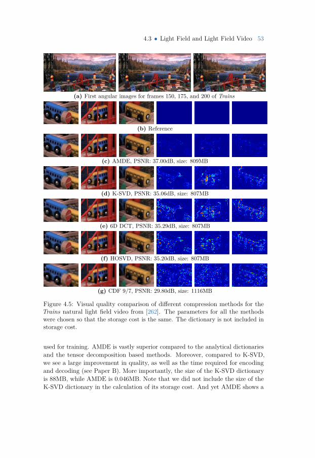
4.3 • Light Field and Light Field Video 53
(a) First angular images for frames 150, 175, and 200 of Trains
(b) Reference
(c) AMDE, PSNR: 37.00dB, size: 809MB
(d) K-SVD, PSNR: 35.06dB, size: 807MB
(e) 6D DCT, PSNR: 35.29dB, size: 807MB
(f) HOSVD, PSNR: 35.20dB, size: 807MB
(g) CDF 9/7, PSNR: 29.80dB, size: 1116MB
Figure 4.5: Visual quality comparison of different compression methods for theTrains natural light field video from [262]. The parameters for all the methodswere chosen so that the storage cost is the same. The dictionary is not included instorage cost.
used for training. AMDE is vastly superior compared to the analytical dictionariesand the tensor decomposition based methods. Moreover, compared to K-SVD,we see a large improvement in quality, as well as the time required for encodingand decoding (see Paper B). More importantly, the size of the K-SVD dictionaryis 88MB, while AMDE is 0.046MB. Note that we did not include the size of theK-SVD dictionary in the calculation of its storage cost. And yet AMDE shows a
54 Chapter 4 • Compression of Visual Data
much superior image quality compared to K-SVD.
For light field videos, we used the dataset described in [262], which was capturedusing a 4×4 camera array at 30 frames per second. Each camera has a resolutionof 2048×1088. From this dataset, we create data points of size m1 = 10, m2 = 10,m3 = 4, m4 = 4, m5 = 3, and m6 = 4; i.e. the spatial patches are 10×10 and eachdata point contains four consecutive frames. Note that we have included all theangular information in each data point to have seamless angular reconstructionduring the rendering. For training, we set the following parameters: C = 4, K = 32,τl = 100, p= 400, and Nr = 6000. The training of AMDE was done on the Painterdataset to compress the Trains dataset, as shown in Fig. 4.5. These two light fieldvideos are visually very different from each other. Moreover, unlike Lytro Illumlight fields (see Fig. 6.5) which have a disparity of 1 to 5 pixels, the disparity of theTrains light field video is up tp 150 pixels. Since there is little coherence along theangular dimension of each data point, the dataset we use here is very challengingfor compression. Here, we also see the clear advantage of the AMDE, achievingabout 2.0dB over K-SVD, even though the size of the K-SVD dictionary is 432MBand the size of the AMDE is 0.0627MB.
Reconstruction of light fields and light field videos is fairly straightforward. Westate the reconstruction procedure for a light field video. Indeed when rendering alight field video, we only need to reconstruct a single light field view in a frame.Let T (i)
x1,x2,...,x6 be an element of T (i) that we would like to reconstruct. Since thedictionaries in the ensemble are orthonormal and the coefficients are sparse, wecan use the following formula to obtain T (i)
x1,x2,...,x6 :
T (i)x1,x2,...,x6 =
zi∑z=1
S(i)lz1 ,lz2 ,...,l
z6U(1,mi)x1,l
z1
U(2,mi)x2,l
z2. . .U(6,mi)
x6,lz6, (4.3)
where m and S(i) are obtained from Algorithm 2, zi is the number of nonzeroelements in S(i), and (lz1, lz2, . . . , lz6) defines the location of nonzero values in S(i).
Since the computational complexity of (4.3) is only related to the sparsity of datapoints, an efficient GPU-based implementation is indeed feasible. We developed anapplication for real time playback of high resolution light field videos, achievingmore than 40 frames per second for the dataset of [262] and 200 frames persecond for the Stanford Lego Gantry dataset using an NVIDIA Titan Xp GPU.The implementation utilizes multi-threading and pixel buffer objects (PBO) toaccelerate the data transfer between the CPU and the GPU, hence enabling realtime playback of lengthy light field videos on a consumer level PC.
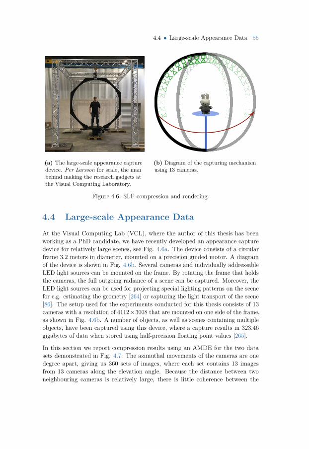
4.4 • Large-scale Appearance Data 55
(a) The large-scale appearance capturedevice. Per Larsson for scale, the manbehind making the research gadgets atthe Visual Computing Laboratory.
(b) Diagram of the capturing mechanismusing 13 cameras.
Figure 4.6: SLF compression and rendering.
4.4 Large-scale Appearance Data
At the Visual Computing Lab (VCL), where the author of this thesis has beenworking as a PhD candidate, we have recently developed an appearance capturedevice for relatively large scenes, see Fig. 4.6a. The device consists of a circularframe 3.2 meters in diameter, mounted on a precision guided motor. A diagramof the device is shown in Fig. 4.6b. Several cameras and individually addressableLED light sources can be mounted on the frame. By rotating the frame that holdsthe cameras, the full outgoing radiance of a scene can be captured. Moreover, theLED light sources can be used for projecting special lighting patterns on the scenefor e.g. estimating the geometry [264] or capturing the light transport of the scene[86]. The setup used for the experiments conducted for this thesis consists of 13cameras with a resolution of 4112×3008 that are mounted on one side of the frame,as shown in Fig. 4.6b. A number of objects, as well as scenes containing multipleobjects, have been captured using this device, where a capture results in 323.46gigabytes of data when stored using half-precision floating point values [265].
In this section we report compression results using an AMDE for the two datasets demonstrated in Fig. 4.7. The azimuthal movements of the cameras are onedegree apart, giving us 360 sets of images, where each set contains 13 imagesfrom 13 cameras along the elevation angle. Because the distance between twoneighbouring cameras is relatively large, there is little coherence between the
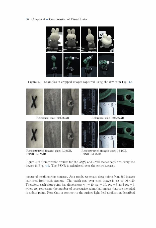
56 Chapter 4 • Compression of Visual Data
Figure 4.7: Examples of cropped images captured using the device in Fig. 4.6
Reference, size: 323.46GB Reference, size: 323.46GB
Reconstructed images, size: 9.39GB,PSNR: 44.71dB
Reconstructed images, size: 9.54GB,PSNR: 46.80dB
Figure 4.8: Compression results for the Miffy and Drill scenes captured using thedevice in Fig. 4.6. The PSNR is calculated over the entire dataset.
images of neighbouring cameras. As a result, we create data points from 360 imagescaptured from each camera. The patch size over each image is set to 40× 30.Therefore, each data point has dimensions m1 = 40, m2 = 30, m3 = 3, and m4 = 6,where m4 represents the number of consecutive azimuthal images that are includedin a data point. Note that in contrast to the surface light field application described
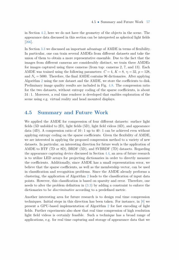
4.5 • Summary and Future Work 57
in Section 4.2, here we do not have the geometry of the objects in the scene. Theappearance data discussed in this section can be interpreted as spherical light fields[266].
In Section 3.3 we discussed an important advantage of AMDE in terms of flexibility.In particular, one can train several AMDEs from different datasets and take theunion of them to obtain a more representative ensemble. Due to the fact that theimages from different cameras are considerably distinct, we train three AMDEsfor images captured using three cameras (from top: cameras 2, 7, and 13). EachAMDE was trained using the following parameters: C = 4, K = 8, τl = 32, p= 128,and Nr = 5000. Therefore, the final AMDE contains 96 dictionaries. After applyingAlgorithm 2 using the raw dataset and the AMDE, we store the coefficients to disk.Preliminary image quality results are included in Fig. 4.8. The compression ratiofor the two datasets, without entropy coding of the sparse coefficients, is about34 : 1. Moreover, a real time renderer is developed that enables exploration of thescene using e.g. virtual reality and head mounted displays.
4.5 Summary and Future WorkWe applied the AMDE for compression of four different datasets: surface lightfields (5D unfolded to 2D), light fields (5D), light field videos (6D), and appearancedata (4D). A compression ratio of 10 : 1 up to 40 : 1 can be achieved even withoutapplying entropy coding on the sparse coefficients. Given the flexibility of AMDE,we are interested in applying the proposed compression method to a variety of newdatasets. In particular, an interesting direction for future work is the application ofAMDE to BTF (7D or 8D), BRDF (5D), and SVBRDF (7D) datasets. Regardingthe appearance capturing device discussed in Section 4.4, an area of future researchis to utilize LED arrays for projecting dictionaries in order to directly measurethe coefficients. Additionally, since AMDE has a small representation error, webelieve that the sparse coefficients, as well as the membership vector, can be usedin classification and recognition problems. Since the AMDE already performs aclustering, the application of Algorithm 2 leads to the classification of input datapoints. However, this classification is based on sparsity and error. Therefore, oneneeds to alter the problem definition in (3.3) by adding a constraint to enforce thedictionaries to be discriminative according to a predefined metric.
Another interesting area for future research is to design real time compressiontechniques. Initial steps in this direction has been taken. For instance, in [8] wepresent a GPU-based implementation of Algorithm 2 for fast encoding of lightfields. Further experiments also show that real time compression of high resolutionlight field videos is certainly feasible. Such a technique has a broad range ofapplications, e.g. for real time capturing and storage of appearance data that we

58 Chapter 4 • Compression of Visual Data
discussed in Section 4.4. While compressed sensing, which is the topic of chapters5 and 6, is a more efficient method to accelerate the capturing of visual data, itrequires different sensing mechanisms, and hence new hardware implementations.In contrast, real time compression during the capturing can be applied on top ofexisting measurement devices for obtaining compact representations of BRDFs,BTFs, light field videos, and other types of visual data.

Ch
ap
te
r
5Compressed Sensing
Figure 5.1: Saving time with mathe-matics1.
For decades, the Shannon-Nyquist theorem[69, 70] defined the requirements for sam-pling signals. It states that a band-limitedsignal with no frequencies higher than f canbe completely determined by placing samplesat uniform (equally spaced) points that are1/2f seconds apart, which implies samplingat a rate of 2f (known as the Nyquist rate).Uniform sampling exerts several limitationsin practice, especially when sampling rate ishigh. The introduction of nonuniform sam-pling [267] opened up many new researchdirections. The Shannon-Nyquist theoremholds for nonuniform sampling as long as theaverage sampling rate exceeds the Nyquistrate [268]. This requirement can be relaxedwhen we know the frequency band locations and their widths [269, 270], or usingperiodic non-uniform sampling [271], as well as reconstruction from local averages[272]. However, reconstruction methods used for uniform sampling do not apply tononuniform sampling (see [273] for a review of recovery methods from nonuniformsamples). Two important applications that deal with the problem of reconstructinga signal from its nonuniform frequency-domain samples are Computed Tomography
1 Image source: people.eecs.berkeley.edu/~mlustig/
60 Chapter 5 • Compressed Sensing
(CT) and Magnetic Resonance Imaging (MRI) [274].
Compressed Sensing sparked a paradigm shift in signal sampling. The main resultsin compressed sensing state that a sparse signal can be exactly recovered with asampling rate well-below the Nyquist rate. While sparse representation was a veryactive field in 1990s and 2000s for denoising and solving inverse problems usingwavelets, mathematical formulation of conditions for exact recovery was neverconsidered [122]. Just like many other ground-breaking inventions, compressedsensing was discovered by chance. In 2004, Emmanuel Candès was trying toreconstruct a sub-sampled Shepp-Logan Phantom image [275]. By his surprise,the result of the `1 problem turned out to be an exact recovery of the originalimage even though the sampling rate was well-below what he thought was therequired number of measurements. This motivated him to find the reason behindthis “magical” outcome and to formulate it. With the help of one of the greatestmathematicians of our time, Terrence Tao, they published some of the seminalworks in compressed sensing [75, 76, 77]. In parallel, David Donoho presented aninformation theoretic perspective on recovery of sparse signals from only a fewmeasurements [42], and for the first time dubbed the method “compressed sensing”.
The majority of the work presented in this thesis involves compressed sensing.Moreover, contributions of this thesis on the topic are both theoretical and empirical.This chapter will discuss the theoretical findings of this thesis, in which an outlineof the materials to be discussed, as well as the contributions, are summarizedin Section 5.1. In Chapter 6, we will present the empirical contributions of thisthesis for utilizing compressed sensing in various computer graphics and imagingapplications.
5.1 Outline and ContributionsCompressed sensing is indeed of paradoxical nature – exact reconstruction fromwhat appears to be highly inadequate measurements. Therefore, rigorous analysis ofthe conditions for exact recovery is crucial. Before presenting the main theoreticalcontributions of this thesis regarding compressed sensing, key definitions that areused throughout this chapter are presented in Section 5.2. Section 5.3 formulatesthe compressed sensing problem for 1D signals, which is the most common way offormulating the problem, as well as nD signals. In addition, we discuss differenttypes of measurement matrices in Section 5.4, which play an important role inderiving conditions for exact recovery. There are two families of theoretical analysisin compressed sensing. Universal theoretical results (Section 5.5) demonstrate theconditions for exact recovery by analyzing the properties of a measurement matrix,sparsity, and the number of measurements. There exists a large body of researchon deriving metrics for the suitability of a measurement matrix with regards to
5.2 • Definitions 61
exact recovery. We will review a number of these metrics in sections 5.5.1–5.5.4and present some of the key results regarding the universal recovery conditions forsparse signals.
Aside from universal results, there exists a family of theoretical results on theconvergence of specific algorithms solving the compressed sensing problem (e.g.using `0, `1, or `p norms for 0 < p < 1). Indeed these algorithm-specific resultsalso consider sparsity, number of measurements, and the metrics on measurementmatrices for exact recovery. However, these properties are considered in the contextof the algorithm at hand. Algorithm-specific analyses typically perform betterfor an specific algorithm than universal results; however this comes at the costof reducing the generality of the obtained theoretical results. This thesis makescontributions by presenting a novel algorithm-specific analysis, as well as a universalresult for recovery of signals that are sparse under a dictionary ensemble.
One of the key contributions of this thesis is a theoretical analysis of OrthogonalMatching Pursuit (OMP), an `0 recovery method that is widely used and providesa good trade off between accuracy and computational cost. In Section 5.6, wedescribe the OMP algorithm and present its advantages and disadvantages from apractical point of view. Next, in Section 5.7, a theoretical analysis of the methodis presented, where we derive conditions under which the OMP algorithm exactlyrecovers a sparse signal. This analysis is a combination of the theoretical resultsreported in Paper F and Paper G.
In Section 5.8, we present a theoretical analysis on the uniqueness of the solutionobtained from an `0 problem when the signal is sparse in an ensemble of dictionaries(see Section 3.2). This analysis is based on a spike ensemble for point sampling,which has several applications in graphics and imaging. The theoretical resultsfor an ensemble of 2D dictionaries (orthogonal or overcomplete) were reported inPaper D. Moreover, a generalized analysis for an ensemble of nD dictionaries waspresented in Paper B. Finally, in Section 5.9 we summarize the contributions andpresent possible venues for future work.
5.2 Definitions
In what follows, a number of key definitions that will be used in the upcomingsections of this chapter are listed.
Definition 5.1 (signal). A signal, in the context of the materials presented inthis thesis, is a real or complex valued vector (x ∈ Rm), matrix (X ∈ Rm1×m2) ortensor (X ∈ Rm1×m2×···×mn).
62 Chapter 5 • Compressed Sensing
Formulations in this chapter are based on real-valued signals, unless stated other-wise.
Definition 5.2 (τ-sparse). A signal x ∈Rm is called τ -sparse under a dictionaryD ∈ Rm×k if x = Ds and ‖s‖0 = τ . Note that τ ≤m, otherwise the representationis not unique. This definition can also be used for vec(X) and vec(X ).
Definition 5.3 ((τ1, . . . , τn)-sparse). A signal X ∈Rm1×···×mn is called (τ1, . . . , τn)-sparse under an nD dictionary
D(i) ∈ Rmi×ki
ni=1
if X = S×1 D(1)×2 · · ·×nD(n)
andmax
∀j∈
1,...,∏nk=1,k 6=jmk
∥∥∥(S(i)):,j∥∥∥
0= τi (5.1)
Note that τi≤mi, ∀i∈ 1, . . . ,n, otherwise the uniqueness of representation cannotbe guaranteed.
Definition 5.4 (support). Let x ∈Rm be τ -sparse under a dictionary D ∈Rm×k.The support of x, denoted supp(x)D, is a set of natural numbers holding the locationof nonzero values in s. When it is clear from the context, we may drop the subscript,i.e. supp(x). For matrices and tensors, the elements of the support set are tuples,e.g. (i1, i2),(j1, j2), . . . and (i1, . . . , in),(j1, . . . , jn), . . ., respectively.
Definition 5.5 (mutual coherence). The mutual coherence of a matrix X ∈Rm×k is
µ(X) = max1≤i6=j≤k
|XTi Xj |
‖Xi‖2‖Xj‖2. (5.2)
Definition 5.6 ((p,q) operator norm). The (p,q) operator norm of a matrix Xis defined as
‖X‖p,q = maxb6=0
‖Xb‖q‖b‖p
(5.3)
5.3 Problem FormulationIn Section 1.2, we briefly introduced compressed sensing and formulated the problemof sampling a 1D sparse signal. For convenience, we include equations (1.1) and(1.2) below
mins‖s‖0 s.t. ‖y−ΦDs‖22 ≤ ε, (5.4)
mins‖s‖1 s.t. ‖y−ΦDs‖22 ≤ ε, (5.5)
where Φ ∈Rs×m is a measurement or sensing matrix and D ∈Rm×k is a dictionarythat enables the sparse representation of an unknown signal x = Ds, ‖s‖0 = τ . Themeasurement model is formulated as y = Φx + w, where w is the measurement
5.4 • The Measurement Matrix 63
noise. The sensing matrix Φ maps a vector of dimension m to a vector of dimensions. The variable s denotes the number of samples, and is typically user-defined,unless the measurement matrix has a predefined size. If the measurements areassumed to be noise-free, i.e. w = 0, then the constraints of (5.4) and (5.5) arereplaced with y = ΦDs. It is a common practice to define A = ΦD for convenience.The matrix A is called an equivalent measurement matrix.
The recovery of an nD signal, X ∈ Rm1×···×mn , that is (τ1, . . . , τn)-sparse under annD dictionary U(1) ∈ Rm1×k1 , . . . ,U(n) ∈ Rmn×kn is formulated as follows
minS
∥∥∥S∥∥∥0
s.t.∥∥∥Y− S×1 Φ(1)U(1)×2 · · ·×nΦ(n)U(n)
∥∥∥2
2≤ ε, (5.6)
whereΦ(1) ∈ Rs1×m1 , . . . ,Φ(n) ∈ Rsn×mn
are measurement matrices that operate
independently along each dimension, and s1, . . . , sn are the number of samplesalong each dimension. Moreover, Y = X ×1 Φ(1)×2 · · ·×nΦ(n) +W defines themeasurement model. It is possible to convert (5.6) to an equivalent 1D form withindependent measurement matrices
mins‖s‖0 s.t.
∥∥∥y−(Φ(n)U(n)⊗·· ·⊗Φ(1)U(1)) s∥∥∥2
2, (5.7)
where y =(Φ(n)⊗·· ·⊗Φ(1))vec(X ). Another possibility is to convert (5.6) to an
equivalent 1D form, however with a single measurement matrix
mins‖s‖0 s.t.
∥∥∥y−Φ(U(n)⊗·· ·⊗U(1)) s
∥∥∥2
2≤ ε, (5.8)
where y = Φvec(X ) and Φ ∈ Rs×(m1m2...mn). An advantage of (5.8) is that thenumber of samples, s, can be fine tuned, whereas in (5.6) and (5.7) the total numberof samples is s= s1s2 . . . sn.
5.4 The Measurement MatrixThere exists numerous choices for populating a measurement matrix, denoted Φ.Two major categories exist in this regard: random and deterministic. Perhapsthe most commonly used random measurement matrix is one with i.i.d. Gaussianentries. These matrices are provably optimal for exact recovery (see Section 5.5.4 formore details). Moreover, Gaussian matrices simplify the analysis of exact recoveryconditions in various cases. Other types of random measurement matrices alsoexist. For instance, we can set the elements of Φ to 0,1 with probability 1/2 (i.e.the symmetric Bernoulli distribution), or to ±1 with probability 1/2. Moreover, ameasurement matrix can be constructed by sampling from the uniform distributionin the interval [0,1], which is essentially equivalent to sampling on the unit sphere
64 Chapter 5 • Compressed Sensing
of Rs. For random sensing matrices, the measurement model y = Φx +w dictatesthat one has to have access to all the elements of x. However, in many applications,we would like to directly sample a subset of elements in x, which is known as pointsampling. For discrete signals, point sampling is modeled by a matrix, definedbelow.
Definition 5.7 (spike ensemble). Let Γ be the uniform random permutationof the set 1, . . . ,m. Define Λ as the first s ≤m entries of Γ. Then the spikeensemble is defined as IΛ,., where I ∈ Rm×m is the identity matrix.
A spike ensemble has a nonzero element in each row. If there exists more than onenonzero element in a row, we obtain a binary sensing matrix [276].
Deterministic measurement matrices are categorized into analytical and learningbased. Analytical matrices are constructed using mathematical tools such thatstrong theoretical guarantees can be achieved for the solution of (5.4) or (5.5); a fewexamples include [277, 278, 279, 280, 281, 282, 283]. On the other hand, learningbased methods use an optimization problem to generate a matrix Φ such that theequivalent measurement matrix A = ΦD produces a more accurate solution to(5.4) or (5.5). A few examples in this category include [284, 285, 286, 287].
There exists an additional family of sensing matrices that have deterministicstructures but may contain random elements. For instance, random circulant andToeplitz matrices have been used for compressed sensing [288, 289, 290, 291, 292].Moreover, the measurement matrix for a single sensor light field camera is block-circulant with random elements. This type of sensing matrix will be described indetail in Section 6.2.
5.5 Universal Conditions for Exact RecoveryUniversal results in compressed sensing state the required conditions for recoveringa sparse signal from incomplete measurements, regardless of the algorithm usedfor solving the problem. Formulating universal results requires the assumptionthat the recovery algorithm converges to a solution. While this is true for the `1formulation (i.e. (5.5)), there is no guarantee that an `0 recovery may lead to themost sparse solution, and that the solution is unique. Hence, universal resultstypically state the equivalence conditions for the solutions of `0 and `1 problems.
5.5.1 Uncertainty Principle and CoherenceHeisenberg’s uncertainty principle states that complementary physical propertiesof a particle, e.g. position and momentum wave functions, cannot be measuredwith arbitrary precision simultaneously. In mathematical terms, let f(x) be any
5.5 • Universal Conditions for Exact Recovery 65
absolutely continuous function such that xf(x) and f ′(x) are square integrable[293]. Moreover, let F (ω) be the Fourier transform of f(x). Uncertainty principlestates that f(x) and F (ω) obey the following inequality
(∫ ∞−∞
x2|f(x)|2dx)(∫ ∞
−∞ω2|F (ω)|2dω
)≥ C, (5.9)
where C is a constant. It can be noted that the integrals above calculate the secondmoments of |f(x)|2 and |F (ω)|2 about zero. This is a well-known property in theclassical sampling literature. For example, a box function in spatial domain is aSinc function in the frequency domain and an impulse train (i.e. point samples)with period T in the spatial domain becomes an impulse train with period 1/T inthe frequency domain.
Let us now translate the discussion above to the language of compressed sensing.Assume that we have a complex-valued signal x∈Cm. Let I∈Rm×m be the identitymatrix and Iα be a subset of columns in I. Note that Iα is a point sampling matrixthat extracts the elements of x corresponding to α. Moreover, let F ∈ Cm×m bethe Fourier transform matrix, and let Fβ be a subset of columns in F. Since both Iand F are orthonormal bases, there exists s(1) and s(2) such that x = Is(1) = Fs(2).In this setup, the uncertainty principle described in [294] shows that the inequality|α|+ |β| ≥ 2
√m holds. In other words, x cannot be sparse in the canonical basis
and the Fourier basis at the same time.
We can also write a sparse representation of x as
x = [I,F]s(1)
s(2)
︸ ︷︷ ︸
s
, (5.10)
where [I,F] is the concatenation of I and F along columns. We now have arrivedat an underdetermined system of linear equation and several questions arise. Forinstance, is it possible to obtain a solution from
mins‖s‖0 s.t. x = [I,F]s, (5.11)
ormin
s‖s‖1 s.t. x = [I,F]s, (5.12)
that is unique (i.e. the global minimizer)? And what is the relation between |α|and |β| in the obtained unique solution? These questions were answered by Donohoand Hue in [295], which is summarize in the following theorem
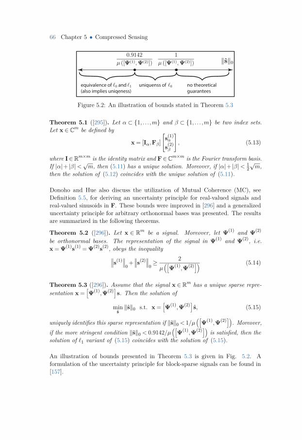
66 Chapter 5 • Compressed Sensing
0.9142
µ ([Ψ(1),Ψ(2)])
1
µ ([Ψ(1),Ψ(2)]) ‖s‖0
no theoretical guarantees
uniquenss of 0equivalence of and (also implies uniqeness)
0 1
Figure 5.2: An illustration of bounds stated in Theorem 5.3
Theorem 5.1 ([295]). Let α ⊂ 1, . . . ,m and β ⊂ 1, . . . ,m be two index sets.Let x ∈ Cm be defined by
x = [Iα,Fβ]s(1)α
s(2)β
, (5.13)
where I∈Rm×m is the identity matrix and F∈Cm×m is the Fourier transform basis.If |α|+ |β|<
√m, then (5.11) has a unique solution. Moreover, if |α|+ |β|< 1
2√m,
then the solution of (5.12) coincides with the unique solution of (5.11).
Donoho and Hue also discuss the utilization of Mutual Coherence (MC), seeDefinition 5.5, for deriving an uncertainty principle for real-valued signals andreal-valued sinusoids in F. These bounds were improved in [296] and a generalizeduncertainty principle for arbitrary orthonormal bases was presented. The resultsare summarized in the following theorems.
Theorem 5.2 ([296]). Let x ∈ Rm be a signal. Moreover, let Ψ(1) and Ψ(2)
be orthonormal bases. The representation of the signal in Ψ(1) and Ψ(2), i.e.x = Ψ(1)s(1) = Ψ(2)s(2), obeys the inequality∥∥∥s(1)
∥∥∥0
+∥∥∥s(2)
∥∥∥0≥ 2µ([
Ψ(1),Ψ(2)]) (5.14)
Theorem 5.3 ([296]). Assume that the signal x ∈ Rm has a unique sparse repre-sentation x =
[Ψ(1),Ψ(2)]s. Then the solution of
mins‖s‖0 s.t. x =
[Ψ(1),Ψ(2)] s, (5.15)
uniquely identifies this sparse representation if ‖s‖0 < 1/µ([
Ψ(1),Ψ(2)]). Moreover,if the more stringent condition ‖s‖0 < 0.9142/µ
([Ψ(1),Ψ(2)]) is satisfied, then the
solution of `1 variant of (5.15) coincides with the solution of (5.15).
An illustration of bounds presented in Theorem 5.3 is given in Fig. 5.2. Aformulation of the uncertainty principle for block-sparse signals can be found in[157].
5.5 • Universal Conditions for Exact Recovery 67
5.5.2 SparkIn Section 5.5.1 we discussed the uniqueness conditions for measurement matricesof the form
[Ψ(1),Ψ(2)], where Ψ(1) and Ψ(2) are orthonormal. However, as
discussed in Section 1.2, measurement matrices are often defined by an overcompletematrix A = ΦD. Therefore, the matrix A is not necessarily a concatenation oforthonormal matrices; for instance let Φ ∈ R
m2 ×m be any sub-sampling of rows
from the identity matrix and D be any orthonormal matrix. The first tool toanalyze such measurement matrices in the context of uniqueness was Spark [73],defined below.
Definition 5.8 (spark). Spark of a matrix A ∈ Rs×k, denoted spark(A), is thesmallest subset of columns in A that are linearly dependent.
Spark of any matrix is bounded by [2,rank(A) + 1]. The lower bound comes fromthe assumption that A does not have a zero-valued column. The upper bound isachieved for e.g. an orthonormal matrix. Note that a full-rank matrix may have aspark of 2. For example, spark([1,I, . . . ]) = 2, where 1 ∈ Rs is a vector of ones ands≥ 2. The matrix [I,F] described in Section 5.5.1 can be shown to have a spark of2√m [73]. Let Φ ∈ Rs×m be an overcomplete matrix with i.i.d. Gaussian elements
and D ∈ Rm×m be an orthonormal matrix. Then spark(ΦD) = s+ 1 [297]. Whilethe spark of certain classes of matrices can be calculated analytically, computingthe spark for general matrices is a combinatorial problem requiring 2k steps for amatrix of size s×k.
Spark can be used for determining the uniqueness of the solution obtained from an`0 problem, as well as the equivalence conditions between `0 and `1 solutions.
Theorem 5.4 ([73]). Assume that a signal y ∈ Rs has a unique sparse representa-tion y = As, for a predefined equivalent measurement matrix A ∈ Rs×k. Then thesolution of
mins‖s‖0 s.t. y = As, (5.16)
is the unique sparsest solution if ‖s‖0 < spark(A)/2. Moreover, given this condition,the solution of the `1 variant of (5.16) coincides with the unique solution of (5.16).
The sparsity upper bound, ‖s‖0 < spark(A)/2, is sharp [73]; i.e. there is no sparsitybound δ > spark(A)/2 that guarantees uniqueness. Moreover, spark and mutualcoherence are related by the inequality spark(A)> 1/µ(A).
5.5.3 Exact Recovery CoefficientExact Recovery Coefficient (ERC) was first introduced by J. Tropp in [79] as ametric for evaluating the performance of OMP and basis pursuit for solving `0
68 Chapter 5 • Compressed Sensing
and `1 problems, respectively. Tropp formulates the recovery conditions for bothτ -sparse and compressible signals. Later, these results were extended in [74] fornoisy signals, and universal recovery conditions were derived. ERC is defined asfollows
Definition 5.9 (ERC). ERC of a matrix A ∈ Rs×k is given by
ERC(Λ) = 1−maxα∈Γ‖A†ΛAα‖1 (5.17)
where Λ⊂ 1, . . . ,k and Γ = 1, . . . ,k\Λ. The symbol \ denotes set difference.
Consider the case where Λ = supp(s) for the system x = As. Hence, ERC measureshow distinct the atoms corresponding to Λ are compared to those that are notin the support. Indeed if there is a distinction, i.e. ERC(Λ) > 0, and the signalis noise free, then various recovery algorithms can find the support [79]. For thecase of noisy signals, i.e. when the measurements are y = As+w, where w is anunknown noise vector, Tropp [74] formulates the following theorem:
Theorem 5.5 ([74]). Assume that an equivalent measurement matrix A ∈ Rs×k
and a measured signal y ∈Rs are given. Let Λ⊂ 1, . . . ,k be an index set such thatthe columns of AΛ are linearly independent and ERC(Λ)> 0. Then the solution sof
mins‖s‖1 s.t. ‖y−As‖2 ≤ ε, (5.18)
is unique and supp(s)⊂ Λ, if
ε≥∥∥∥y−AΛA†Λy
∥∥∥2
√√√√√√1 +
δ∥∥∥A†Λ∥∥∥2,1
ERC(Λ)
2
, (5.19)
where
δ =max
i∈1,...,k
(y−AΛA†Λy
)TAi∥∥∥y−AΛA†Λy
∥∥∥ , (5.20)
and ‖.‖2,1 is defined in (5.3). Moreover, the representation error is bounded by
‖s− s∗‖2 ≤ δ‖A†Λ‖F , (5.21)
where s∗ is the optimal sparse vector.
5.5.4 Restricted Isometry ConstantRestricted isometry constant was first introduced in [76] and it is defined as follows
5.5 • Universal Conditions for Exact Recovery 69
Definition 5.10 (RIC). Let A ∈ Rs×k and τ ∈ 1, . . . , s. Restricted isometryconstant δτ of A is the smallest number such that
(1− δτ )‖s‖22 ≤ ‖As‖22 ≤ (1 + δτ )‖s‖22, (5.22)
holds for all τ -sparse signals s.
Equation 5.22 can also be expressed as
δτ = maxΛ⊂1,...,s, |Λ|≤τ
‖ATΛAT
Λ− I‖2,2, (5.23)
where ‖.‖2,2 is the spectral norm of a matrix; i.e. ‖X‖2,2 = λmax(X). RIC hasseveral implications. From (5.23) we see that the smaller the RIC, δτ , the closer AΛis to an orthogonal matrix (for all possible sets Λ⊂ 1, . . . , s, |Λ| ≤ τ). Moreover,equation (5.23) shows that δ2 = µ(A) and that the singular values of AΛ are in[1− δτ ,1 + δτ ]. Finally, according to (5.22), if δ2τ is sufficiently small, this meansthat the distances between τ -sparse signals under the transformation A is wellpreserved:
(1− δ2τ )‖s(1)− s(2)‖22 ≤ ‖As(1)−As(2)‖22 ≤ (1 + δ2τ )‖s(1)− s(2)‖22. (5.24)
Loosely speaking, we say that A satisfies the Restricted Isometry Property (RIP)if δτ is sufficiently small. When RIP holds, the solution of the `0 program is uniqueand coincides with the solution of the `1 program. More concretely,
Theorem 5.6 ([298]). Consider the measurement model y = As+w, where A ∈Rs×k and w is an unknown noise vector. Assume that δ2τ <
√2−1 and ‖w‖2 ≤ ε.
Then the solution ofmin
s‖s‖1 s.t. ‖y−As‖2 ≤ ε, (5.25)
satisfies‖s− s‖2 ≤
C0√τ‖s− so‖1 +C1ε, (5.26)
where C0 and C1 are constants that only depend on δ2τ , and so is a solution obtainedfrom the oracle estimator, i.e. one that knows the location of nonzero entries in s.
The bound δ2τ <√
2− 1 has been improved several times [299, 300, 301, 302].Although RIC is NP-hard to compute, it can be shown that certain classes ofmeasurement matrices satisfy RIP, as described in Theorem 5.6. For instance, if theelements of A are i.i.d. Gaussian random variables with mean zero and variance1/s, then A satisfies RIP with overwhelming probability if s≥ Cτ log (k/τ), whereC is a constant [78]. The same applies if the columns of A are sampled uniformlyat random on the unit sphere of Rs.
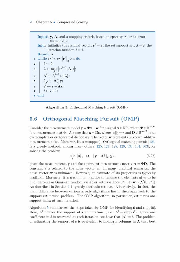
70 Chapter 5 • Compressed Sensing
Input: y, A, and a stopping criteria based on sparsity, τ , or an errorthreshold, ε.
Init.: Initialize the residual vector, r0 = y, the set support set, Λ = ∅, theiteration number, i= 1.
Result: s1 while i≤ τ or
∥∥∥ri∥∥∥2> ε do
2 s← 0;3 λ←max
j
∣∣∣〈ri−1,Aj〉∣∣∣;
4 Λi← Λi−1∪λ;5 sΛi ←A+
Λiy;6 ri← y−As;7 i← i+ 1;8 end
Algorithm 5: Orthogonal Matching Pursuit (OMP)
5.6 Orthogonal Matching Pursuit (OMP)Consider the measurement model y = Φx+w for a signal x ∈Rm, where Φ∈Rs×m
is a measurement matrix. Assume that x = Ds, where ‖s‖0 = τ and D∈Rm×k is anovercomplete or orthonormal dictionary. The vector w represents unknown additivemeasurement noise. Moreover, let Λ = supp(s). Orthogonal matching pursuit [126]is a greedy method, among many others [125, 127, 128, 129, 133, 134, 303], forsolving the problem
mins‖s‖0 s.t. ‖y−As‖2 ≤ ε, (5.27)
given the measurements y and the equivalent measurement matrix A = ΦD. Theconstant ε is related to the noise vector w. In many practical scenarios, thenoise vector w is unknown. However, an estimate of its properties is typicallyavailable. Moreover, it is a common practice to assume the elements of w to bei.i.d. zero-mean Gaussian random variables with variance σ2, i.e. w∼N (0,σ2I).As described in Section 1.1, greedy methods estimate Λ iteratively. In fact, themain difference between various greedy algorithms lies in their approach to thesupport estimation problem. The OMP algorithm, in particular, estimates onesupport index at each iteration.
Algorithm 5 summarizes the steps taken by OMP for identifying s and supp(s).Here, Λi defines the support of s at iteration i, i.e. Λi = supp(si). Since onecoefficient in s is recovered at each iteration, we have that |Λi|= i. The problemof estimating the support of s is equivalent to finding k columns in A that best
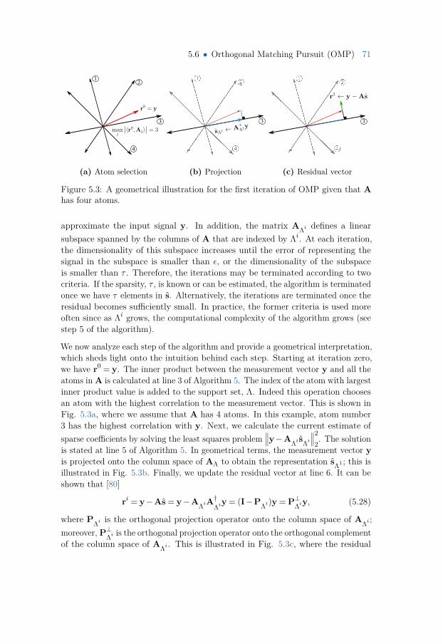
5.6 • Orthogonal Matching Pursuit (OMP) 71
12
3
4
(a) Atom selection
12
3
4
(b) Projection
12
3
4
(c) Residual vector
Figure 5.3: A geometrical illustration for the first iteration of OMP given that Ahas four atoms.
approximate the input signal y. In addition, the matrix AΛi defines a linearsubspace spanned by the columns of A that are indexed by Λi. At each iteration,the dimensionality of this subspace increases until the error of representing thesignal in the subspace is smaller than ε, or the dimensionality of the subspaceis smaller than τ . Therefore, the iterations may be terminated according to twocriteria. If the sparsity, τ , is known or can be estimated, the algorithm is terminatedonce we have τ elements in s. Alternatively, the iterations are terminated once theresidual becomes sufficiently small. In practice, the former criteria is used moreoften since as Λi grows, the computational complexity of the algorithm grows (seestep 5 of the algorithm).
We now analyze each step of the algorithm and provide a geometrical interpretation,which sheds light onto the intuition behind each step. Starting at iteration zero,we have r0 = y. The inner product between the measurement vector y and all theatoms in A is calculated at line 3 of Algorithm 5. The index of the atom with largestinner product value is added to the support set, Λ. Indeed this operation choosesan atom with the highest correlation to the measurement vector. This is shown inFig. 5.3a, where we assume that A has 4 atoms. In this example, atom number3 has the highest correlation with y. Next, we calculate the current estimate ofsparse coefficients by solving the least squares problem
∥∥∥y−AΛi sΛi∥∥∥2
2. The solution
is stated at line 5 of Algorithm 5. In geometrical terms, the measurement vector yis projected onto the column space of AΛ to obtain the representation sΛ1 ; this isillustrated in Fig. 5.3b. Finally, we update the residual vector at line 6. It can beshown that [80]
ri = y−As = y−AΛiA†Λi
y = (I−PΛi)y = P⊥Λiy, (5.28)
where PΛi is the orthogonal projection operator onto the column space of AΛi ;moreover, P⊥Λi is the orthogonal projection operator onto the orthogonal complementof the column space of AΛi . This is illustrated in Fig. 5.3c, where the residual
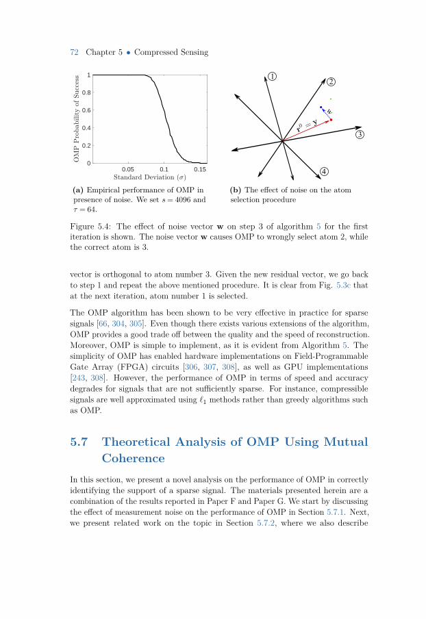
72 Chapter 5 • Compressed Sensing
0.05 0.1 0.150
0.2
0.4
0.6
0.8
1
(a) Empirical performance of OMP inpresence of noise. We set s= 4096 andτ = 64.
12
3
4
w
(b) The effect of noise on the atomselection procedure
Figure 5.4: The effect of noise vector w on step 3 of algorithm 5 for the firstiteration is shown. The noise vector w causes OMP to wrongly select atom 2, whilethe correct atom is 3.
vector is orthogonal to atom number 3. Given the new residual vector, we go backto step 1 and repeat the above mentioned procedure. It is clear from Fig. 5.3c thatat the next iteration, atom number 1 is selected.
The OMP algorithm has been shown to be very effective in practice for sparsesignals [66, 304, 305]. Even though there exists various extensions of the algorithm,OMP provides a good trade off between the quality and the speed of reconstruction.Moreover, OMP is simple to implement, as it is evident from Algorithm 5. Thesimplicity of OMP has enabled hardware implementations on Field-ProgrammableGate Array (FPGA) circuits [306, 307, 308], as well as GPU implementations[243, 308]. However, the performance of OMP in terms of speed and accuracydegrades for signals that are not sufficiently sparse. For instance, compressiblesignals are well approximated using `1 methods rather than greedy algorithms suchas OMP.
5.7 Theoretical Analysis of OMP Using MutualCoherence
In this section, we present a novel analysis on the performance of OMP in correctlyidentifying the support of a sparse signal. The materials presented herein are acombination of the results reported in Paper F and Paper G. We start by discussingthe effect of measurement noise on the performance of OMP in Section 5.7.1. Next,we present related work on the topic in Section 5.7.2, where we also describe
5.7 • Theoretical Analysis of OMP Using Mutual Coherence 73
why mutual coherence is a suitable candidate for the analysis of OMP. Our novelanalysis of OMP is presented in Section 5.7.3, followed by numerical results inSection 5.7.4.
5.7.1 The Effect of Noise on OMP
An important aspect affecting the accuracy of OMP is the measurement noise, w.A large amount of noise can lead to incorrect atom selection (at line 3 of Algorithm5). Figure 5.4b demonstrates this effect for iteration 0. The Gaussian noise isshown with a green circle, where the CDF is illustrated with a color gradient.Because the noise is additive, i.e. y = As+w, it moves the residual vector to a newrandom point (shown in blue). As it can be seen, at this new location, OMP willchoose atom 2 instead of 3. Hence, it is essential to quantify the tolerance of OMPto noise for correct atom selection. This is one of the contributions of this thesis,which will be described in detail in Section 5.7.3. Figure 5.4a shows the empiricalprobability of support recovery for OMP with respect to the standard deviation ofthe noise vector. In this plot, for a fixed value of σ, the probability of success iscalculated as the number of successful support recoveries among 5000 trials, wherein each trial we instantiate a new sparse signal and noise vector. It can be seenthat increasing the noise quickly decreases the probability of support recovery.
Since greedy algorithms solve an `0 problem, e.g. equation (5.27), it cannot beguaranteed (in general) that an optimal solution can be obtained. This is in contrastwith `1 algorithms, which solve a convex problem with a guaranteed convergenceto the global minimum. Moreover, the addition of noise to measurements furthercomplicates the analysis of convergence. As described in Section 5.6, OMP iscomputationally efficient and competitive in terms of accuracy, while enablingsimple implementations. As a result, a substantial amount of work has beendedicated for obtaining theoretical guarantees for the convergence of OMP.
5.7.2 Prior Art and Motivation
Tropp analyzed the convergence of OMP using ERC in [79]. Various extensionsof this work exists. For instance, partial-ERC was introduced in [309, 310] forsolving (5.27) when the support is partially known. Restricted isometry propertyhas been used extensively for the analysis of OMP [80, 311, 312, 313, 314]. Wangand Shim [315] utilize RIP to derive the required number of OMP iterations forexact recovery and Ding et al. [316] derive sufficient conditions using RIP whenboth the signal y and the measurement matrix A are perturbed (noisy). Sparkhas not directly been used for OMP analysis. However, performance guaranteesusing spark (e.g. Theorem 5.4) do apply to OMP.
74 Chapter 5 • Compressed Sensing
While RIC, ERC, and spark provide accurate performance guarantees, and in somecases even sharp conditions, these constants cannot be computed in practice for alarge family of measurement matrices. Computing ERC is a combinatorial problemthat is often intractable for large measurement matrices. In general, computingRIC and spark for arbitrary measurement matrices is NP-hard [317]. We discussedin Section 5.5 that these constants can only be computed (or bounded) for asmall subset of random or deterministic matrices. In contrast, mutual coherence issimple to compute and has a complexity of O(sk2) for a matrix A ∈ Rs×k. This isparticularly important for training-based dictionaries, since it is difficult, and mostof the times impossible, to compute RIC, ERC, and spark. For instance, assumethat D is trained using the K-SVD algorithm (described in Section 2.4), and Φ isa spike ensemble. The equivalent sensing matrix, A, is deterministic and there areno closed-form solutions for obtaining RIP, ERC, or spark.
One of the early works on deriving coherence-based performance guarantees forOMP was presented in [18]. Theorem 5.7 below presents the main result of [18].Without loss of generality, we assume that the columns of A are normalized.
Theorem 5.7 ([18]). Let y = As+w, where A∈Rs×k, ‖s‖0 = τ and w∼N (0,σ2I).Define smin = min
j|sj |. If
smin− (2τ −1)µ(A)smin ≥ 2β, (5.29)
where β =∆ σ√
2(1 +α) logk is defined for some constant α > 0, then with probabilityat least
1− 1kα√π(1 +α) logk
, (5.30)
OMP identifies the true support of s.
The proof of Theorem 5.7 is based on analyzing the event Pr|〈Aj ,w〉| ≤ β,∀j ∈ 1, . . . ,k. Hence the correlation of the noise vector with the atoms of Ais considered. Indeed if this correlation is too large, i.e. when the noise vectordominates the signal, then step 3 in Algorithm 5 will select an incorrect atom (seeFig. 5.4b). Hence, Ben-Haim et al. [18] analyze the probability that the noisecorrelation is bounded. Equation (5.30) is in fact a lower bound for the eventPr|〈Aj ,w〉| ≤ β. Therefore, we see that the probability of support recovery,(5.30), is decoupled from important parameters related to s and A such as smin, τ ,and µ(A). These parameters affect the condition in (5.29); hence if the conditionfails, equation (5.30) is invalid. Moreover, smax = max
j|sj | is not considered. In
many applications, smax and smin are known or can be estimated. For instance, inimaging applications one can obtain bounds on the values of the sparse signal sbecause the original signal, x, is typically in [0,1] to facilitate quantization. The
5.7 • Theoretical Analysis of OMP Using Mutual Coherence 75
ratio of the largest and smallest signal values is known as the Dynamic Range (DR)of a signal.
5.7.3 A Novel Analysis Based on the Concentration ofMeasure
Paper F presents a performance guarantee for the exact support recovery of a noisysignal using OMP and mutual coherence. By identifying the shortcomings in theresults of [18], the proposed analysis contains signal parameters in the probabilitybound and is shown to better match the empirical results. We state the main resultbelow.
Theorem 5.8 (Paper F). Let y = As + w, where A ∈ Rs×k, τ = ‖s‖0 and w ∼N (0,σ2I). Moreover, assume that the nonzero elements of s are independentcentered random variables with an arbitrary distribution. If smin/2≥ β, for someconstant β ≥ 0, then OMP identifies the true support with lower bound probability1−k
√2π
σ
βe−β
2/2σ2
(1−2k exp(
−k(smin/2−β)2
2τ2γ2 + 2kγ(smin/2−β)/3
)), (5.31)
where γ = µ(A)smax.
Before presenting the proof, we will summarize important implications of Theorem5.8 in the following remarks.
Remark 5.1. A key factor that distinguishes Theorem 5.8 from Theorem 5.7 isthe assumption of i.i.d. random variables in s, as opposed to the assumption ofdeterministic variables. This is by no means a limiting factor since we do notassume the distribution of these variables. Most importantly, randomness of nonzerovalues in s enables us to use concentration inequalities in the proof of Theorem 5.8,which greatly simplifies the analysis and provides a more accurate probability bound.
Remark 5.2. The probability bound in (5.31) contains two terms: The first term isrelated to the noise properties and the signal length, while the second term is relatedto the signal and dictionary properties. This is in sharp contrast with Theorem5.7, where a condition is imposed on the signal and dictionary properties, while theprobability bound only considers the noise related factors and the signal length.
Remark 5.3. The condition smin/2≥ β of Theorem (5.8) is far less stringent than(5.29). Moreover, numerical simulations show that smin/2≥ β is satisfied for anyreasonable choice of parameters.
Remark 5.4. We observe that the first term of (5.31) is equivalent to (5.30). Thiscan be shown by replacing β in the first term of (5.31) with σ
√2(1 +α) logk, which
76 Chapter 5 • Compressed Sensing
is the value used for β in Theorem 5.7. Since the second term of (5.31) is in[0,1], this implies that (5.30) is always larger than (5.31). However, the conditionimposed by Theorem 5.7 is not satisfied for a large range of parameters. Thismeans that (5.30) is not valid in many cases, for which (5.31) may evaluate to highprobabilities.
A sketch of the proof for Theorem 5.8 is presented below and the reader is referredto Paper F for more details.
Proof sketch for Theorem 5.8. Ben-Haim et al. show that if the event Pr|〈Aj ,w〉| ≤β holds, then OMP identifies the true support, Λ, if [18]
minj∈Λ|〈Aj ,AΛsΛ +w〉| ≥max
k/∈Λ|〈Ak,AΛsΛ +w〉|. (5.32)
Simple manipulations of (5.32) yieldsmaxi/∈ΛΓi<min
j∈Λ
|sj |2 ,
maxj∈Λ
∣∣∣〈Aj ,AΛ\jsΛ\j+w〉∣∣∣<min
j∈Λ
|sj |2 ,
(5.33)
where Γi = |〈Ai,As+w〉|. In fact we have broken (5.32) into two (joint) conditionsfor successful recovery. The first one checks whether the maximum correlation ofatoms in the support with y (or the residual) is smaller than smin. The secondone checks whether the maximum correlation of atom j in the support with themeasurement vector y, excluding atom j, is smaller than smin. From (5.33), anupper bound for the probability of error can be obtained
Prerror ≤∑j∈Λ
Pr∣∣∣〈Aj ,AΛ\jsΛ\j+w〉
∣∣∣≥ smin2
+∑i/∈Λ
Pr
Γi ≥smin
2
.
(5.34)We now bound the two terms on the right-hand side of (5.34), excluding thesummations. For the second term we have
Pri/∈Λ
Γi ≥
smin2
≤ 2 exp
−(smin/2−β)2
2(τ2γ
2
k + γ(smin/2−β)3 )
︸ ︷︷ ︸
P2
. (5.35)
Equation (5.35) is obtained by expanding Γi to form a sum of random variables,followed by the application of the Bernstein inequality [318], which is one theseveral concentration inequalities [319] for sum of random variables. A similar
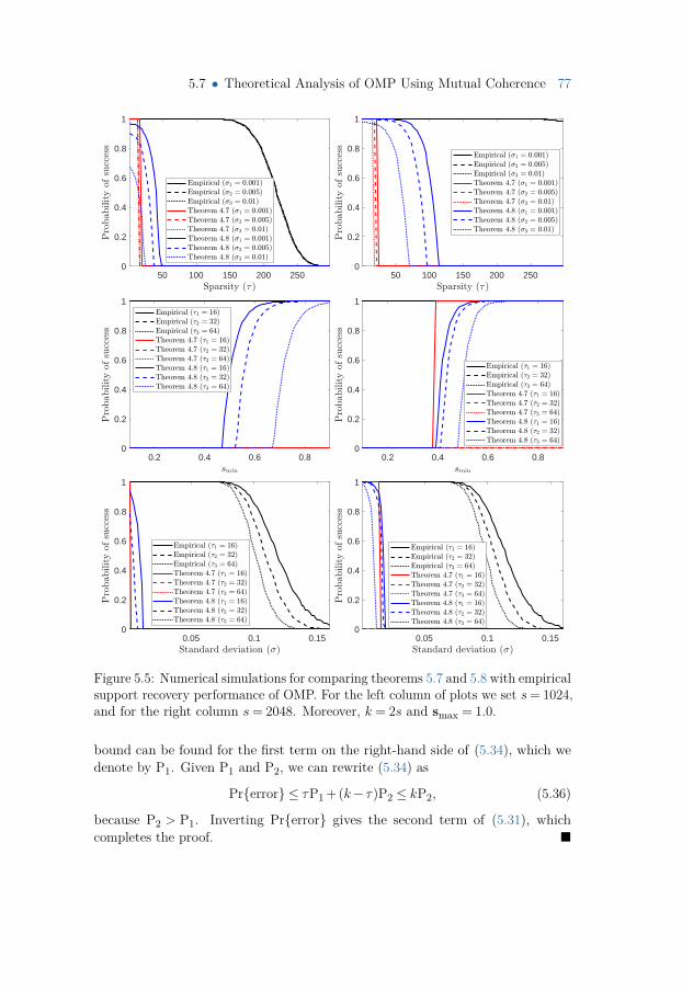
5.7 • Theoretical Analysis of OMP Using Mutual Coherence 77
50 100 150 200 2500
0.2
0.4
0.6
0.8
1
50 100 150 200 2500
0.2
0.4
0.6
0.8
1
0.2 0.4 0.6 0.80
0.2
0.4
0.6
0.8
1
0.2 0.4 0.6 0.80
0.2
0.4
0.6
0.8
1
0.05 0.1 0.150
0.2
0.4
0.6
0.8
1
0.05 0.1 0.150
0.2
0.4
0.6
0.8
1
Figure 5.5: Numerical simulations for comparing theorems 5.7 and 5.8 with empiricalsupport recovery performance of OMP. For the left column of plots we set s= 1024,and for the right column s= 2048. Moreover, k = 2s and smax = 1.0.
bound can be found for the first term on the right-hand side of (5.34), which wedenote by P1. Given P1 and P2, we can rewrite (5.34) as
Prerror ≤ τP1 + (k− τ)P2 ≤ kP2, (5.36)
because P2 > P1. Inverting Prerror gives the second term of (5.31), whichcompletes the proof.
78 Chapter 5 • Compressed Sensing
5.7.4 Numerical Results
Numerical simulations for comparing Theorem 5.8 and Theorem 5.7, as well asempirical results of OMP are summarized in Fig. 5.5. The empirical probabilitywas obtained by performing OMP 5000 times, where in each trial a random sparsesignal (i.e. random support and random nonzero elements) and a random noisevector w were constructed. The probability of success is the ratio of successfultrials in identifying the support of s to the total number of trials. The measurementmatrix used here is A = [I,H], where H is the Hadamard matrix. For theorems5.7 and 5.8, we fix the value of β to facilitate comparison. It can be seen that thecondition (5.29) is not satisfied for a large range of parameters, specifically whensmin is small (i.e. high dynamic range), τ is large, or σ is large. Most importantly,the shape of the probability curve produced by Theorem 5.8 is similar to that ofOMP, while Theorem 5.7 produces a step function.
5.7.5 User-friendly Bounds
Theorem 5.8 states the probability of recovering the support of s. In absence ofnoise, once we have recovered the correct support, the signal s can be exactlyreconstructed (see (2.14)). However, in presence of noise, the estimates of nonzerosignal values, sΛ, are not exact. Fortunately, we can derive an estimate of the errorintroduced by the noise. The following theorem states an upper bound for theabsolute error of the solution obtained from OMP, assuming that the support isrecovered correctly.
Theorem 5.9 ([65] and Paper G). Using the same setup as in Theorem 5.8, assumethat OMP identifies the true support of s. Then the error of the estimated sparsesignal with respect to s is upper bounded by
Eabs =∆ ‖s− s‖22 ≤τβ2
(1−µmax(τ −1))2 , (5.37)
In what follows, it will be shown that by combining theorems 5.8 and 5.9, we canobtain approximate, but user-friendly, bounds that depend on the parameterscommonly used in practice. Moreover, this analysis sheds light on the effect ofdifferent parameters on the two terms of (5.31), see Remark 5.2. The resultsreported in this section are from Paper G; however, here we reformulate theseresults for real-values signals.
Define the dynamic range, Signal to Noise Ratio (SNR), and the relative error,respectively as follows
5.8 • Uniqueness Under a Dictionary Ensemble 79
DR =∆(smaxsmin
)2, (5.38)
SNR =∆(sminσ
)2, (5.39)
Erel =∆ Eabs∑Nn=1 sn
≤ Eabsτs2
min. (5.40)
Using simple calculations, Paper G shows that (5.31) can be approximated as
(1−k
√2
πρ2ErelSNRe−Erelρ
2SNR/2)1−2k exp
−18τ2
µ2DRk + 4µ
√DR
3
, (5.41)
where we define ρ2 = (1−µ(τ −1))2 and µ= µ(A) for notational brevity. Assumethat SNR is very high, then the first term of (5.41) becomes close to 1 and can beomitted. In this case, the probability of support recovery is lower bounded by
1−2k exp
−18τ2
µ2DRk + 4µ
√DR
3
. (5.42)
We have now obtained a bound that is only dependent on the signal properties andthe equivalent measurement matrix. Let us now consider the case when µ is verysmall. Note that µ= 0 only holds for matrices with orthogonal columns. A lowerbound for mutual coherence of overcomplete matrices is
√(k− s)[s(k−1)]−1. For
instance, a two times overcomplete matrix A ∈R1000×2000, has a mutual coherenceof at least µ(A) = 2.24e−5. This lower bound can be achieved for e.g. A = [I,F]or A = [I,H], where F is the Fourier transform matrix and H is the Hadamardmatrix. When mutual coherence is small, we can approximate (5.41) as
1−N√
2πErelSNRe
−ErelSNR/2. (5.43)
As it can be seen, equation (5.43) is independent of DR. This is expected becausewhen the mutual coherence is low, atoms of A are far apart, so that the DR doesnot affect the atom selection process.
5.8 Uniqueness Under a Dictionary EnsembleSo far we have described selected fundamental results in compressed sensingfor one dictionary (Section 5.5), as well as some of the contributions of this

80 Chapter 5 • Compressed Sensing
thesis regarding exact recovery with OMP for signals that are sparse under anovercomplete dictionary (Section 5.7). These theoretical results suggest that thehigher the sparsity of a signal, the higher the probability of exact recovery. Asdescribed in Chapter 1, natural signals are not typically sparse, but compressible.In practical applications, small coefficients of a compressible signal are nullified toobtain a sparse signal, which indeed introduces error in the representation. For afixed signal (e.g. an image), it is the effectiveness of the dictionary that defines therepresentation error. The ensemble of dictionaries introduced in sections 3.2 and3.3 was empirically shown to promote sparsity by performing consecutive clusteringand dictionary training. As it will be seen in Chapter 6, this increase in sparsityimproves the performance of compressed sensing. It remains to be seen that whena dictionary ensemble is used for compressed sensing, can the uniqueness of theobtained solution be guaranteed? How many samples are needed for exact recovery?These questions are answered in Paper D and Paper B, which are also the focus ofthis section.
In Section 5.8.1, we formulate a compressed sensing problem for the case whenthe unknown signal that we would like to reconstruct is sparse in an ensemble ofdictionaries. Next, in Section 5.8.2, we define uniqueness for the solution obtainedfrom an ensemble of dictionaries using compressed sensing. A key theoreticalcontribution of this thesis regarding the aforementioned problem is presented inSection 5.8.3. Finally, we discuss the results of numerical simulations obtainedfrom the proposed theoretical analysis in Section 5.8.4.
5.8.1 Problem FormulationLet Ψ =
D(d)D
d=1be an ensemble of dictionaries, where D(d) ∈Rm×k. A training
based method for obtaining an ensemble of multidimensional orthonormal dictionar-ies was discussed in Section 3.3. In this section, we do not assume any structure onthese dictionaries; i.e. each dictionary can be orthogonal, overcomplete, with i.i.d.Gaussian entries, learned, deterministic, or analytical. Furthermore, we convertmultidimensional dictionaries to their equivalent 1D form. This can be simplyachieved using the Kronecker product as follows
D(d) =∆ U(n,d)⊗·· ·⊗U(1,d), ∀d ∈ 1, . . . ,D, (5.44)
whereU(1,d), . . . ,U(n,d)D
d=1is an ensemble of nD dictionaries. Hence, the `1
sparse recovery problem using an ensemble can be formulated as
mins,D∈Ψ
‖s‖1 s.t. ‖x−Ds‖2 ≤ ε. (5.45)
In other words, we need to solve (5.45) for all the dictionaries in Ψ and pick themost sparse solution. Indeed a successful recovery requires that the signal x has
5.8 • Uniqueness Under a Dictionary Ensemble 81
a unique sparse representation among all the dictionaries. In other words, onedictionary in Ψ should lead to the most sparse representation. If two or moredictionaries produce a solution with the same sparsity for x, then uniqueness cannotbe guaranteed. Uniqueness of the solution of (5.45) will be defined more concretelyin Section 5.8.2.
We can (theoretically) construct an ensemble such that a signal x has a uniquesparse representation. The training algorithm described in Section 3.2 learnsan ensemble such that a signal is sparse in only one dictionary. However, theoptimization problem is highly nonlinear, hence being trapped in a local minimais inevitable. Note that (5.45) is a sparse representation problem rather thancompressed sensing. Even if we can construct an optimal ensemble, the equivalentmeasurement matrix A = ΦD(d) may lead to multiple sparse representations thathinders the uniqueness of the solution obtained from
mins,D∈Ψ
‖s‖1 s.t. ‖y−ΦDs‖2 ≤ ε, (5.46)
where y = Φx.
5.8.2 Uniqueness DefinitionWe now formulate the uniqueness conditions for a dictionary ensemble Ψ. Weassume that there exists a unique solution to problem (5.46) for any of the dictio-naries in Ψ. This can be verified with the metrics described in Section 5.5. Forinstance, using spark, it is required that spark
(ΦD(i)) > 2τ for any dictionary
D(i) ∈Ψ and τ -sparse signal x. Without this assumption, guaranteeing uniquenessfor all the dictionaries can quickly become intractable. Let D(i) and D(j) be anytwo dictionaries in Ψ. Assume that x has a unique sparse representation in D(i),i.e. x = D(i)s(i), where ‖s‖0 = τ and y = ΦD(i)s(i). Uniqueness of the solutionof (5.46) is guaranteed if there is no x 6= x, where x = D(j)s(j) and ‖s(j)‖0 = τ ,that also satisfies y = ΦD(j)s(j). Gleichman and Eldar [297] propose the followingmetric to verify the uniqueness under a dictionary ensemble.
Definition 5.11 (τ-rank preserving [297]). A measurement matrix Φ is calledτ -rank preserving of a dictionary ensemble Ψ if for any index sets I and J withcardinality not larger than τ , and any two dictionaries D(i) ∈Ψ and D(j) ∈Ψ, thefollowing equality holds
rank(Φ[D(i)I ,D
(j)J
])= rank
([D(i)I ,D
(j)J
]). (5.47)
Verifying Definition 5.11 is indeed difficult since all the possibilities of I and J forany two dictionaries have to be assessed. Gleichman and Eldar [297] show that an
82 Chapter 5 • Compressed Sensing
i.i.d. Gaussian matrix Φ is almost surely τ -rank preserving of an ensemble of bases(matrices with linearly independent columns). Formally,
Theorem 5.10 ([297]). Assume that Φ ∈ Rs×m, where s ≤m, is a matrix withi.i.d. Gaussian entries and Ψ =
D(d) ∈ Rm×k
Dd=1
is a finite set of bases. Then,Φ is almost surely τ -rank preserving of the set Ψ. Furthermore, if spark(ΦD)> 2τfor any dictionary D∈Ψ, and Φ is τ -rank preserving, then the most sparse solutionof (5.46), denoted s∗, gives the unique solution x = D∗s∗, where D∗ ∈Ψ is thedictionary that gives s∗.
It remains to be seen if other types of sensing matrices are τ -rank preserving.
5.8.3 Uniqueness with a Spike EnsembleIn Paper D, we present a new analysis for uniqueness under an ensemble ofdictionaries when a spike ensemble (see Definition 5.7) is used for sensing. We firstobserve that a spike ensemble does not satisfy (5.47) for an arbitrary dictionaryensemble, and therefore uniqueness cannot be guaranteed. Hence, a probabilisticanalysis for uniqueness is proposed, where a lower bound on successful recoverybased on the number of samples and the ensemble Ψ is derived. Moreover, thenew analysis removes the requirement of having an ensemble of bases. As a result,even an ensemble of overcomplete dictionaries can be used. Before presenting themain result below, a few notations are introduced. The function orth(X) definesthe orthogonalization of the columns of X, using e.g. QR decomposition [217]. Weuse supp(p)D to denote the support of a signal p under a dictionary D. Indeed afixed signal has variable support under different dictionaries.
Theorem 5.11 (Paper D). Assume that a signal x ∈Rm is at most τ -sparse underall dictionaries in Ψ =
D(d) ∈ Rm×k
Dd=1
, where
τ ≤ 12
1 + 1µ(IΛ,.D
) , ∀D ∈Ψ, (5.48)
or
τ <spark
(IΛ,.D
)2 , ∀D ∈Ψ, (5.49)
is satisfied for a fixed spike ensemble IΛ,. ∈ Rs×m. Let
α = maxj=1,...,m
∥∥∥∥orth([A.,I ,B.,J ]
)j,.
∥∥∥∥2
2, ∀A,∀B ∈Ψ, A 6= B, (5.50)
r = rank([A.,I ,B.,J ]
), (5.51)
I = supp(x)A , A ∈Ψ, (5.52)J = supp(x)B , B ∈Ψ. (5.53)
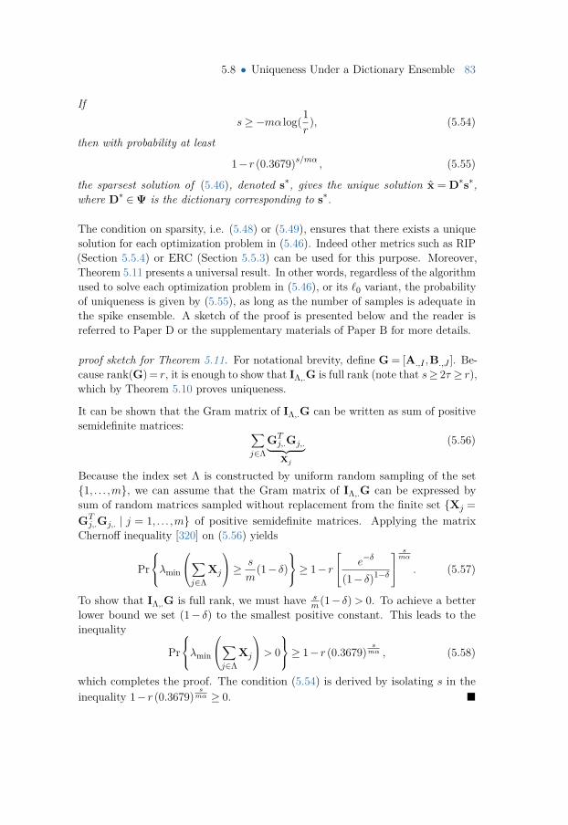
5.8 • Uniqueness Under a Dictionary Ensemble 83
Ifs≥−mα log(1
r), (5.54)
then with probability at least
1− r (0.3679)s/mα , (5.55)
the sparsest solution of (5.46), denoted s∗, gives the unique solution x = D∗s∗,where D∗ ∈Ψ is the dictionary corresponding to s∗.
The condition on sparsity, i.e. (5.48) or (5.49), ensures that there exists a uniquesolution for each optimization problem in (5.46). Indeed other metrics such as RIP(Section 5.5.4) or ERC (Section 5.5.3) can be used for this purpose. Moreover,Theorem 5.11 presents a universal result. In other words, regardless of the algorithmused to solve each optimization problem in (5.46), or its `0 variant, the probabilityof uniqueness is given by (5.55), as long as the number of samples is adequate inthe spike ensemble. A sketch of the proof is presented below and the reader isreferred to Paper D or the supplementary materials of Paper B for more details.
proof sketch for Theorem 5.11. For notational brevity, define G = [A.,I ,B.,J ]. Be-cause rank(G) = r, it is enough to show that IΛ,.G is full rank (note that s≥ 2τ ≥ r),which by Theorem 5.10 proves uniqueness.
It can be shown that the Gram matrix of IΛ,.G can be written as sum of positivesemidefinite matrices: ∑
j∈ΛGTj,.Gj,.︸ ︷︷ ︸Xj
(5.56)
Because the index set Λ is constructed by uniform random sampling of the set1, . . . ,m, we can assume that the Gram matrix of IΛ,.G can be expressed bysum of random matrices sampled without replacement from the finite set Xj =GTj,.Gj,. | j = 1, . . . ,m of positive semidefinite matrices. Applying the matrix
Chernoff inequality [320] on (5.56) yields
Prλmin
∑j∈Λ
Xj
≥ s
m(1− δ)
≥ 1− r e−δ
(1− δ)1−δ
smα
. (5.57)
To show that IΛ,.G is full rank, we must have sm(1− δ)> 0. To achieve a better
lower bound we set (1− δ) to the smallest positive constant. This leads to theinequality
Prλmin
∑j∈Λ
Xj
> 0≥ 1− r (0.3679)
smα , (5.58)
which completes the proof. The condition (5.54) is derived by isolating s in theinequality 1− r (0.3679)
smα ≥ 0.
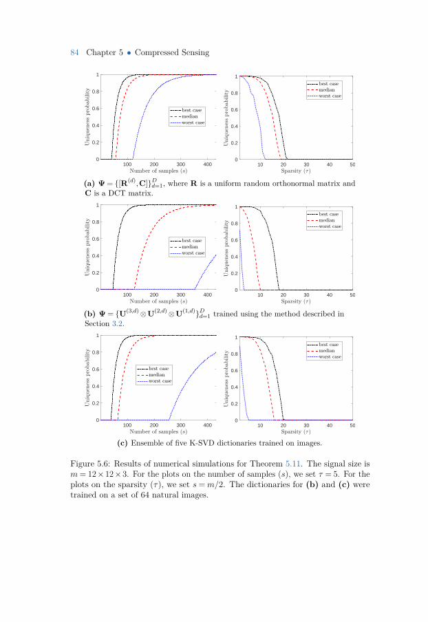
84 Chapter 5 • Compressed Sensing
100 200 300 4000
0.2
0.4
0.6
0.8
1
10 20 30 40 500
0.2
0.4
0.6
0.8
1
(a) Ψ = [R(d),C]Dd=1, where R is a uniform random orthonormal matrix andC is a DCT matrix.
100 200 300 4000
0.2
0.4
0.6
0.8
1
10 20 30 40 500
0.2
0.4
0.6
0.8
1
(b) Ψ = U(3,d)⊗U(2,d)⊗U(1,d)Dd=1 trained using the method described inSection 3.2.
100 200 300 4000
0.2
0.4
0.6
0.8
1
10 20 30 40 500
0.2
0.4
0.6
0.8
1
(c) Ensemble of five K-SVD dictionaries trained on images.
Figure 5.6: Results of numerical simulations for Theorem 5.11. The signal size ism= 12×12×3. For the plots on the number of samples (s), we set τ = 5. For theplots on the sparsity (τ), we set s=m/2. The dictionaries for (b) and (c) weretrained on a set of 64 natural images.
5.9 • Summary and Future Work 85
5.8.4 Numerical Results
In Fig. 5.6 below, we report results for the numerical simulation of Theorem 5.11.The signal size is m = 12× 12× 3, which corresponds to patches of size 12× 12that are extracted from color images. Three types of dictionary ensembles areconsidered. Figure 5.6a reports results for an ensemble of concatenated dictionariesΨ = [R(d),C]Dd=1, where R is a uniform random orthonormal matrix and C isa DCT matrix. Figure 5.6b uses an MDE trained with the method described inSection 3.2 and Fig. 5.6c uses an ensemble of five K-SVD dictionaries trained on aset of natural images. To calculate the probability of uniqueness using (5.55), 105
trials are performed, where in each trial we randomly construct the support sets Iand J , as well as the spike ensemble IΛ,.. Moreover, two dictionaries are chosen atrandom from Ψ in each trial. The plots in Fig. 5.6 present the best case, worstcase, and the median of trials.
5.9 Summary and Future Work
In this chapter, we introduced compressed sensing, a modern approach for samplingand reconstruction of sparse signals. It was shown that a sparse signal can bereconstructed from what appears to be highly inadequate nonadaptive samples. Anumber of important metrics that are used for evaluating the conditions of exactrecovery were discussed. Using these metrics, as well as signal and measurementparameters, we formulated the conditions for exact recovery of a sparse signal.The recovery metrics we introduced in this chapter constitute a small number ofseminal works in compressed sensing. There exists a large number of improvementsover the metrics we described, as well as other types of analyses that introducenew metrics. Moreover, we reviewed the OMP algorithm, which is considered toprovide a good balance between computational complexity and accuracy in sparsesignal recovery.
A key contribution of this thesis, i.e. exact recovery conditions for OMP, waspresented. In particular, a lower bound probability for successful support recovery ofa sparse signal with additive white Gaussian noise was formulated. We also showedthat by using an upper bound for the recovery error, one can obtain simplifiedformulas that reveal the effect of important signal parameters such as dynamicrange and signal to noise ratio on the probability of support recovery. Numericalsimulations of the derived theoretical guarantees show a much closer match toempirical performance of OMP than previous work. Another key contribution ofthis thesis was presented in this chapter, namely the uniqueness conditions for therecovery of a point-sampled signal that is sparse under an ensemble of dictionaries.It was shown that, regardless of the type of dictionaries in the ensemble, it is
86 Chapter 5 • Compressed Sensing
possible to find a unique solution. We formulated a lower bound on the number ofsamples, as well as a lower bound on the probability of successful recovery.
There are several venues for future work. With regards to the theoretical resultson OMP, we believe that the probability bound can be improved to better matchthe empirical results. While the proposed probability bound is significantly moreaccurate than previous work, there exists a considerable gap between our theoreticalresults and the empirical performance of OMP. There exists crude approximationsin the proof of Theorem 5.8 that can be improved, albeit at the cost of loosing thesimplicity of the analysis. Additionally, we only considered additive white Gaussiannoise. In many applications, the noise model is more sophisticated. For instance,the noise in an image obtained from a DLSR camera is a combination of severalnoise types such as read-out noise, photon shot noise, etc. An interesting directionfor future research is to extend the results of Paper F to include different typesof measurement noise. In Section 6.5, we will discuss other possible directions forfuture work with regards to utilizing the theoretical results of Paper F and Paper Gin practice.
Theorem 5.11 presented a novel analysis for the uniqueness conditions of signalsthat are sparse in an ensemble of dictionaries. The current formulation relies on 1Dsignals (vectors). Hence, a multidimensional dictionary ensemble is converted toan equivalent 1D ensemble using (2.10) prior to utilizing the theorem. We believethat a new theoretical analysis that is tailored for an ensemble of multidimensionaldictionaries is an interesting venue for future work. For instance, consider thefollowing compressed sensing problem
minS, U(1,d)
,...,U(n,d)∈Ψ
∥∥∥S∥∥∥0
s.t.∥∥∥Y−S×1 Φ(1)U(1,d)×2 · · ·×nΦ(n)U(n,d)
∥∥∥2
2≤ ε,
(5.59)where Ψ =
U(1,d), . . . ,U(n,d)D
d=1. Problems such as (5.59) have not been con-
sidered yet and there are several unsolved problems. Training an ensemble ofdictionaries that enables sparse representation and performs well in equation (5.59)is an open problem. Another one is to derive performance guaranteed for (5.59)given an ensemble. Can the uniqueness analysis in Theorem 5.11 be adapted to(5.59) without the need for converting the problem to a 1D equivalent form? Notethat Theorem 5.11 is valid for ensembles of any dimensionality when converted tothe equivalent 1D form. However, it may be possible to derive a more accurateprobability bound that is tailored for multidimensional ensembles.
Another direction for future research is to extend Theorem 5.11 to noisy signals.This is particularly important since Theorem 5.11 can be used for designingimaging systems such as light field cameras, which are prone to measurement noise.Moreover, we can include the effect of the representation error in our analysis.

5.9 • Summary and Future Work 87
Recall that the visual data are typically compressible and not sparse. Convertinga compressible signal to a sparse signal introduces error (which is a part of lossycompression techniques we described in Chapter 3). In Theorem 5.11 we assumedthat the signal is sparse in all the dictionaries, which may not be true for somesignals in practice. Therefore, including the effect of noise and representation errorcan greatly improve the applicability of Theorem 5.11 in practice. The combinedeffect of the measurement noise and the representation error can be formulatedusing an upper bound on the total error of reconstruction.

Ch
ap
te
r
6Compressed Sensing in Graphics and
Imaging
So far we have considered theoretical aspects of compressed sensing. Indeed themain goal of this field is to derive conditions under which one can exactly recovera sparse signal from what appears to be incomplete measurements. At the sametime, because compressed sensing deals with the fundamental problem of samplingand reconstruction, it has found numerous applications in substantially differentfields of science and engineering. While this thesis focuses on the applicationsof compressed sensing in computer graphics and image processing, the followingsubjects exemplify the diversity of research fields that use compressed sensing:wireless sensor networks [321, 322], face/gesture/speech recognition [63, 323, 324,325], biomedical applications [326, 327], radar imaging [328, 329], integrated circuits[330, 331, 332], audio source separation [333, 334], and many more.
One of the early applications of compressed sensing was in imaging, specifically the“single pixel camera” [83]. Figure 6.1 demonstrates a block diagram of a single pixelcamera. This imaging system consists of an array of digital micro-mirror devices(DMD) that can be individually addressed. A random number generator createsa random pattern on the DMD array for each shot. The incident light from thescene is reflected off of the random DMD array and integrated at a single photodiode. An analog to digital converter then creates a bit stream which is fed to an `1reconstruction algorithm. The original work reports acceptable image quality from1300 measurements, which is 50 times less than the Nyquist rate. The single pixelcamera has been extended to accommodate active illumination [335], multispectral

90 Chapter 6 • Compressed Sensing in Graphics and Imaging
Photodiode
Scene A/D Bitstream
Reconstruction
Random DMDArray
Figure 6.1: Block diagram of a single pixel camera.
imaging [336, 337], video capture [338], microscopy [339], and terahertz imaging[340]. Another important application of compressed sensing in imaging is MRI,which was first introduced in [26]. Moreover, compressed sensing has been used forfunctional MRI [341, 342, 343, 344], and dynamic MRI [88, 345, 346, 347, 348, 349].For a review of compressed sensing algorithms that can be used in dynamic MRIsee [350].
Inverse problems in image processing can also be formulated using compressedsensing. Assume that an image is multiplied by a linear operator Φ which degradesthe image. The operator Φ may add noise, blur, or subsample the image. Theinverse of these operations are called denoising, deblurring, and super-resolution,respectively. Note that Φ can also be a combination of different operators. If theimage is sparse, then the process of inverting the operator Φ to get back the originalimage is equivalent to solving (5.4) or (5.5). Compressed sensing has been usedextensively for denoising [351, 352, 353, 354], deblurring [355, 356, 357, 358, 359],and super-resolution [360, 361, 362, 363].
To the best of the author’s knowledge, compressed sensing was first used in graphicsfor the acquisition of light transport of a scene [86]. The authors propose to projectrandom illumination patterns onto a scene and perform measurements using acamera. The measurements are then used to reconstruct the light transport matrixusing a modified version of ROMP [303]. Displays and projection systems have alsoutilized compressed sensing [364, 365]. Wang et al. [352] introduced a compressedsensing method for separating noise and features from polygonal meshes. Hue etal. [366] have used compressed sensing for addressing the many-lights problem inrendering. By taking a few measurements from the lighting matrix (that containsillumination information from virtual point lights to points in a scene), the authorsshow that a faithful recovery of the full matrix is possible. Unfortunately there are
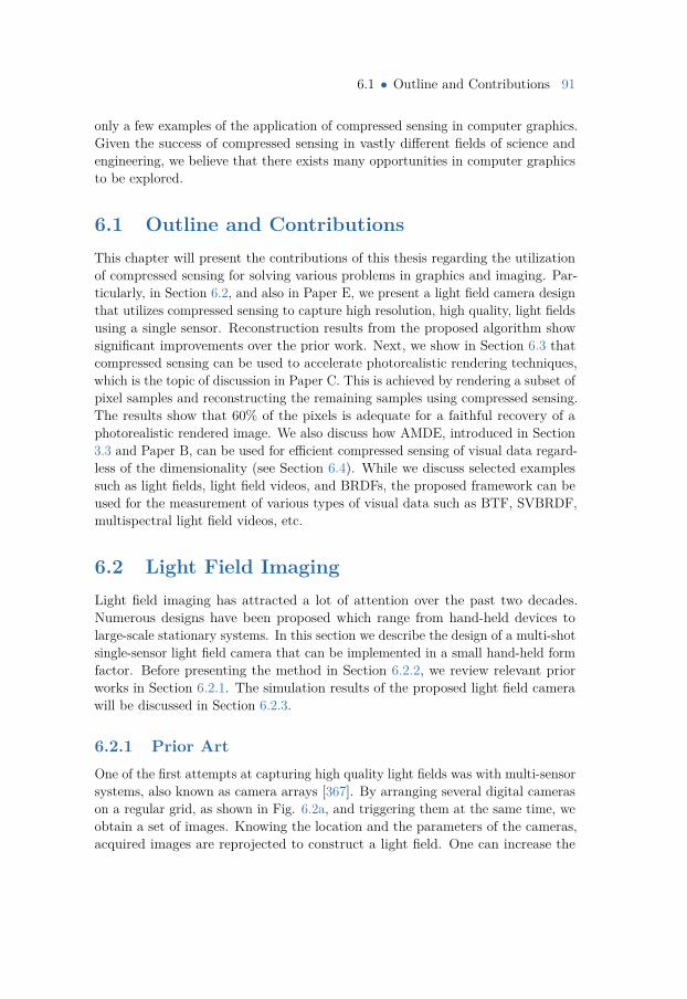
6.1 • Outline and Contributions 91
only a few examples of the application of compressed sensing in computer graphics.Given the success of compressed sensing in vastly different fields of science andengineering, we believe that there exists many opportunities in computer graphicsto be explored.
6.1 Outline and ContributionsThis chapter will present the contributions of this thesis regarding the utilizationof compressed sensing for solving various problems in graphics and imaging. Par-ticularly, in Section 6.2, and also in Paper E, we present a light field camera designthat utilizes compressed sensing to capture high resolution, high quality, light fieldsusing a single sensor. Reconstruction results from the proposed algorithm showsignificant improvements over the prior work. Next, we show in Section 6.3 thatcompressed sensing can be used to accelerate photorealistic rendering techniques,which is the topic of discussion in Paper C. This is achieved by rendering a subset ofpixel samples and reconstructing the remaining samples using compressed sensing.The results show that 60% of the pixels is adequate for a faithful recovery of aphotorealistic rendered image. We also discuss how AMDE, introduced in Section3.3 and Paper B, can be used for efficient compressed sensing of visual data regard-less of the dimensionality (see Section 6.4). While we discuss selected examplessuch as light fields, light field videos, and BRDFs, the proposed framework can beused for the measurement of various types of visual data such as BTF, SVBRDF,multispectral light field videos, etc.
6.2 Light Field ImagingLight field imaging has attracted a lot of attention over the past two decades.Numerous designs have been proposed which range from hand-held devices tolarge-scale stationary systems. In this section we describe the design of a multi-shotsingle-sensor light field camera that can be implemented in a small hand-held formfactor. Before presenting the method in Section 6.2.2, we review relevant priorworks in Section 6.2.1. The simulation results of the proposed light field camerawill be discussed in Section 6.2.3.
6.2.1 Prior ArtOne of the first attempts at capturing high quality light fields was with multi-sensorsystems, also known as camera arrays [367]. By arranging several digital camerason a regular grid, as shown in Fig. 6.2a, and triggering them at the same time, weobtain a set of images. Knowing the location and the parameters of the cameras,acquired images are reprojected to construct a light field. One can increase the
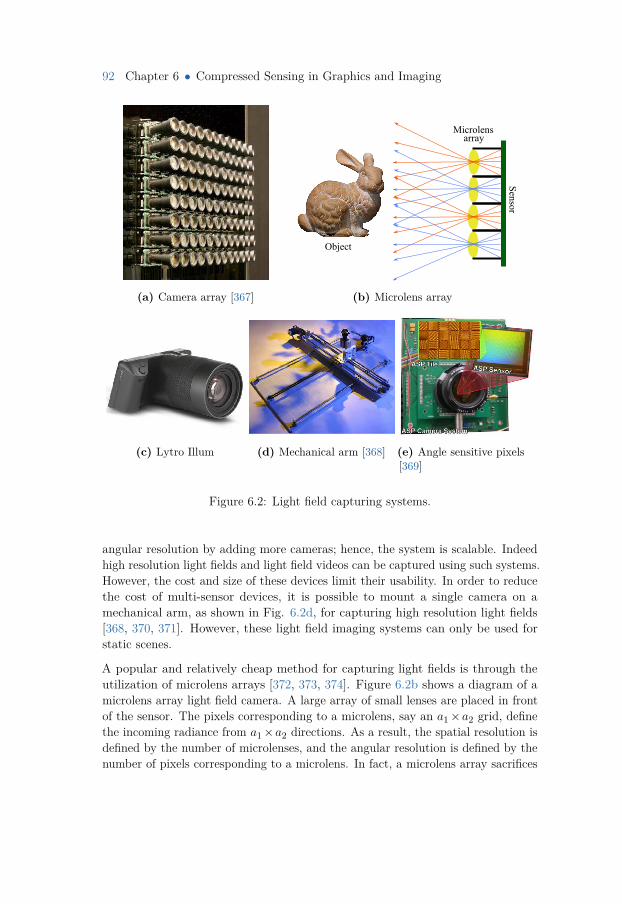
92 Chapter 6 • Compressed Sensing in Graphics and Imaging
(a) Camera array [367]
Sensor
Microlensarray
Object
(b) Microlens array
(c) Lytro Illum (d) Mechanical arm [368] (e) Angle sensitive pixels[369]
Figure 6.2: Light field capturing systems.
angular resolution by adding more cameras; hence, the system is scalable. Indeedhigh resolution light fields and light field videos can be captured using such systems.However, the cost and size of these devices limit their usability. In order to reducethe cost of multi-sensor devices, it is possible to mount a single camera on amechanical arm, as shown in Fig. 6.2d, for capturing high resolution light fields[368, 370, 371]. However, these light field imaging systems can only be used forstatic scenes.
A popular and relatively cheap method for capturing light fields is through theutilization of microlens arrays [372, 373, 374]. Figure 6.2b shows a diagram of amicrolens array light field camera. A large array of small lenses are placed in frontof the sensor. The pixels corresponding to a microlens, say an a1×a2 grid, definethe incoming radiance from a1×a2 directions. As a result, the spatial resolution isdefined by the number of microlenses, and the angular resolution is defined by thenumber of pixels corresponding to a microlens. In fact, a microlens array sacrifices
6.2 • Light Field Imaging 93
spatial resolution of the sensor for angular resolution. Due to the fact that themicrolens light field cameras are small in size and simple to implement, they werethe first to be commercialized (see Fig. 6.2c). However, existing cameras have alow spatial resolution. Recently, a new sensor technology was introduced, namelyan array of angle sensitive pixels (ASP) [375, 376]. Each ASP is tuned to have apredefined angular response by utilizing the Talbot effect. Using computationalphotography, it is possible to obtain a light field from an array of ASPs [369].
Another method for single sensor light field photography is coded aperture [377],where a randomly transparent non-refractive mask is placed on the aperture plane.In this way, each aperture region corresponding to a mask cell transmits a view ofthe scene modulated by the value of the mask cell. Hence the sensor integratesrandomly modulated views of the light field. Knowing the transmittance values ofthe mask, it is possible to reconstruct the light field views. In [378], a programmablemask is placed at the aperture plane. This enables taking multiple shots whilechanging the pattern of the mask, hence increasing the number of samples andimproving the image quality. However, this comes at the cost of long exposuretimes and a large number of shots. A dual mask light field camera was proposed in[379]. While the method increases spatial resolution, the utilization of two masksseverely reduces the light transmission to the sensor. Babacan et al. [85] utilizecompressed sensing to solve the inverse problem of obtaining a light field fromcoded aperture measurements.
More recently, Marwah et al. [17] propose a compressive light field camera wherethe mask is placed at a small distance, dm, from the sensor. Let the functionl(ri,tj ,uα,vβ) be a discrete two plane light field parametrization defined by a pairof locations on the image plane, (ri,tj), and the aperture plane, (uα,vβ). Thenthe image formed on the sensor, denoted y(ri,tj), is obtained by
y(ri,tj) =|u|∑α=1
|v|∑β=1
f(ri+γ(uα− ri),tj +γ(vβ− tj)
)l(ri,tj ,uα,vβ), (6.1)
where f(.) defines the random mask, and γ = dm/da, where da is the distance fromthe sensor to the aperture plane. Equation (6.1) is equivalent to
y =[Φ(1) Φ(2) . . . Φ(ν)
]x(1)
x(2)
...x(ν)
, (6.2)
where ν = |u||v| and Φ(i) ∈ Rω×ω, ω = |r||t|, is a diagonal matrix that containssheared mask values from f(.). Moreover, x(i) ∈ Rω contains a light field viewimage. By assuming sparsity of the light field in the K-SVD dictionary, the authors
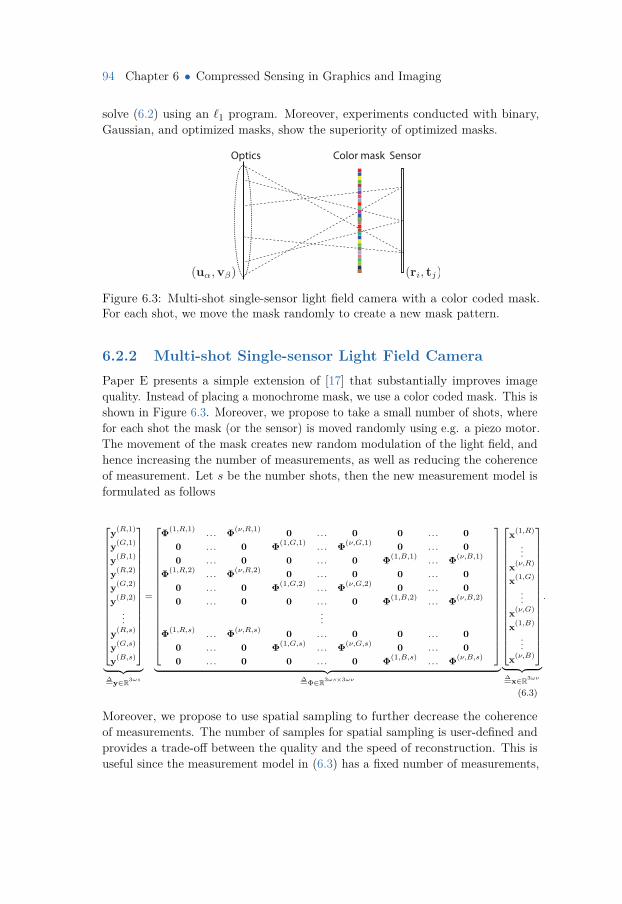
94 Chapter 6 • Compressed Sensing in Graphics and Imaging
solve (6.2) using an `1 program. Moreover, experiments conducted with binary,Gaussian, and optimized masks, show the superiority of optimized masks.
Optics Color mask Sensor
Figure 6.3: Multi-shot single-sensor light field camera with a color coded mask.For each shot, we move the mask randomly to create a new mask pattern.
6.2.2 Multi-shot Single-sensor Light Field CameraPaper E presents a simple extension of [17] that substantially improves imagequality. Instead of placing a monochrome mask, we use a color coded mask. This isshown in Figure 6.3. Moreover, we propose to take a small number of shots, wherefor each shot the mask (or the sensor) is moved randomly using e.g. a piezo motor.The movement of the mask creates new random modulation of the light field, andhence increasing the number of measurements, as well as reducing the coherenceof measurement. Let s be the number shots, then the new measurement model isformulated as follows
y(R,1)
y(G,1)
y(B,1)
y(R,2)
y(G,2)
y(B,2)
...y(R,s)
y(G,s)
y(B,s)
︸ ︷︷ ︸=∆y∈R3ωs
=
Φ(1,R,1). . . Φ(ν,R,1) 0 . . . 0 0 . . . 0
0 . . . 0 Φ(1,G,1). . . Φ(ν,G,1) 0 . . . 0
0 . . . 0 0 . . . 0 Φ(1,B,1). . . Φ(ν,B,1)
Φ(1,R,2). . . Φ(ν,R,2) 0 . . . 0 0 . . . 0
0 . . . 0 Φ(1,G,2). . . Φ(ν,G,2) 0 . . . 0
0 . . . 0 0 . . . 0 Φ(1,B,2). . . Φ(ν,B,2)
...Φ(1,R,s)
. . . Φ(ν,R,s) 0 . . . 0 0 . . . 00 . . . 0 Φ(1,G,s)
. . . Φ(ν,G,s) 0 . . . 00 . . . 0 0 . . . 0 Φ(1,B,s)
. . . Φ(ν,B,s)
︸ ︷︷ ︸
=∆Φ∈R3ωs×3ων
x(1,R)
...x(ν,R)
x(1,G)
...x(ν,G)
x(1,B)
...x(ν,B)
︸ ︷︷ ︸=∆x∈R3ων
.
(6.3)
Moreover, we propose to use spatial sampling to further decrease the coherenceof measurements. The number of samples for spatial sampling is user-defined andprovides a trade-off between the quality and the speed of reconstruction. This isuseful since the measurement model in (6.3) has a fixed number of measurements,
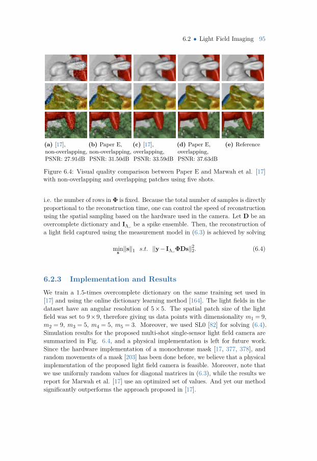
6.2 • Light Field Imaging 95
(a) [17],non-overlapping,PSNR: 27.91dB
(b) Paper E,non-overlapping,PSNR: 31.50dB
(c) [17],overlapping,PSNR: 33.59dB
(d) Paper E,overlapping,PSNR: 37.63dB
(e) Reference
Figure 6.4: Visual quality comparison between Paper E and Marwah et al. [17]with non-overlapping and overlapping patches using five shots.
i.e. the number of rows in Φ is fixed. Because the total number of samples is directlyproportional to the reconstruction time, one can control the speed of reconstructionusing the spatial sampling based on the hardware used in the camera. Let D be anovercomplete dictionary and IΛ,. be a spike ensemble. Then, the reconstruction ofa light field captured using the measurement model in (6.3) is achieved by solving
mins ‖s‖1 s.t. ‖y− IΛ,.ΦDs‖22. (6.4)
6.2.3 Implementation and Results
We train a 1.5-times overcomplete dictionary on the same training set used in[17] and using the online dictionary learning method [164]. The light fields in thedataset have an angular resolution of 5× 5. The spatial patch size of the lightfield was set to 9×9, therefore giving us data points with dimensionality m1 = 9,m2 = 9, m3 = 5, m4 = 5, m5 = 3. Moreover, we used SL0 [82] for solving (6.4).Simulation results for the proposed multi-shot single-sensor light field camera aresummarized in Fig. 6.4, and a physical implementation is left for future work.Since the hardware implementation of a monochrome mask [17, 377, 378], andrandom movements of a mask [203] has been done before, we believe that a physicalimplementation of the proposed light field camera is feasible. Moreover, note thatwe use uniformly random values for diagonal matrices in (6.3), while the results wereport for Marwah et al. [17] use an optimized set of values. And yet our methodsignificantly outperforms the approach proposed in [17].
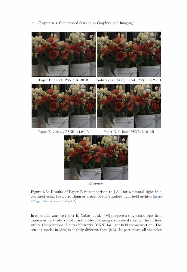
96 Chapter 6 • Compressed Sensing in Graphics and Imaging
Paper E, 1 shot, PSNR: 39.30dB Nabati et al. [380], 1 shot, PSNR: 39.23dB
Paper E, 2 shots, PSNR: 44.95dB Paper E, 5 shots, PSNR: 50.91dB
Reference
Figure 6.5: Results of Paper E in comparison to [380] for a natural light fieldcaptured using the Lytro Illum as a part of the Stanford light field archive (http://lightfields.stanford.edu/).
In a parallel work to Paper E, Nabati et al. [380] propose a single-shot light fieldcamera using a color coded mask. Instead of using compressed sensing, the authorsutilize Convolutional Neural Networks (CNN) for light field reconstruction. Thesensing model in [380] is slightly different than (6.3). In particular, all the color

6.2 • Light Field Imaging 97
Paper E, 1 shot, PSNR: 32.80dB Paper E, 2 shots, PSNR: 38.21dB
Paper E, 5 shots, PSNR: 44.96dB Reference
Figure 6.6: Results of Paper E for a natural light field captured using Lytro Illumas a part of the Stanford light field archive (http://lightfields.stanford.edu/).
channels are measured into a single measurement. The measurement model in (6.3)using combined color sensing becomes
y(1)
y(2)
...y(s)
︸ ︷︷ ︸=∆y∈Rωs
=
Φ(1,R,1)
. . . Φ(ν,R,1) Φ(1,G,1). . . Φ(ν,G,1) Φ(1,B,1)
. . . Φ(ν,B,1)
Φ(1,R,1). . . Φ(ν,R,2) Φ(1,G,2)
. . . Φ(ν,G,2) Φ(1,B,2). . . Φ(ν,B,2)
...Φ(1,R,s)
. . . Φ(ν,R,s) Φ(1,G,s). . . Φ(ν,G,s) Φ(1,B,s)
. . . Φ(ν,B,s)
︸ ︷︷ ︸
=∆Φ∈Rωs×3ων
x. (6.5)
We compare our results with that of [380] in Fig. 6.5 for a natural light fieldcaptured using the Lytro Illum, where the measurement model is according to (6.5).Using one shot, our method achieves a slightly higher PSNR than [380]. However,a visual comparison shows that our method reproduces colors more accurately andis sharper in general. With two shots, our method achieves 5.72db over [380] inPSNR. It should be noted that it is unclear if [380] can be extended for multi-shotlight field capture since the mask is used during training. Using 5 shots, we achieve
98 Chapter 6 • Compressed Sensing in Graphics and Imaging
near-perfect reconstruction and the PSNR gap with [380] becomes 11.68dB. In Fig.6.6, we present another example of a natural light field reconstructed using theproposed light field camera of Paper E.
6.3 Accelerating Photorealistic RenderingPhotorealistic rendering has been a longstanding goal in computer graphics. Withthe advent of ray tracing [249, 250] and accurate surface reflectance modeling[381, 382], a large number of rendering techniques have emerged to progressivelyimprove photorealism and computational cost of rendered images. Some examplesof rendering techniques are: bidirectional path tracing [383, 384], photon mapping[385, 386, 387], and metropolis light transport [388, 389, 390, 391]. While theadvances in rendering techniques and the ever increasing computational powerhave enabled a steady increase in photorealism of rendered images, photorealisticrendering of complex scenes still requires anywhere between minutes to hours, oreven days of computing. We expect this problem to persist in the future sincemore and more physically accurate models for rendering will be utilized to improvephotorealism. In this section, we present an image-based method that can beutilized on top of any rendering technique to accelerate the rendering process. Westart by discussing a number of relevant works on the topic of accelerating therendering process in sections 6.3.1 and 6.3.2. Our proposed method in Paper Cwill be described briefly in Section 6.3.3, followed by the results in Section 6.3.4.
6.3.1 Prior ArtDue to the high dimensionality of the rendering problem, Monte Carlo methods havebeen a key mathematical tool in solving the rendering equation. It is well-knownthat the error of a Monte Carlo estimator goes to zero, almost surely, as the numberof samples goes to infinity. Due to the limited amount of computational power,noise or variance in the produced images are a part of photorealistic renderingtechniques. Hence, rendering methods are typically evaluated based on the qualityof the images produced versus the required number of samples. There exists severalmethods for improving the efficiency of rendering techniques given a fixed budgetof samples. One method is to adaptively sample the space of parameters. In otherwords, we can distribute the fixed number of samples to parameters that contributemore to the quality of the rendered image. While this approach reduces noise, itcan introduce bias in the estimator. A comprehensive review of adaptive samplingmethods is presented in [392]. A different approach is to render using a small numberof samples and then denoise the resulting estimated image [393, 394, 395, 396, 397].An advantage of this method is that it is independent of the rendering algorithmand can be applied on top of adaptive sampling techniques. Another image-based
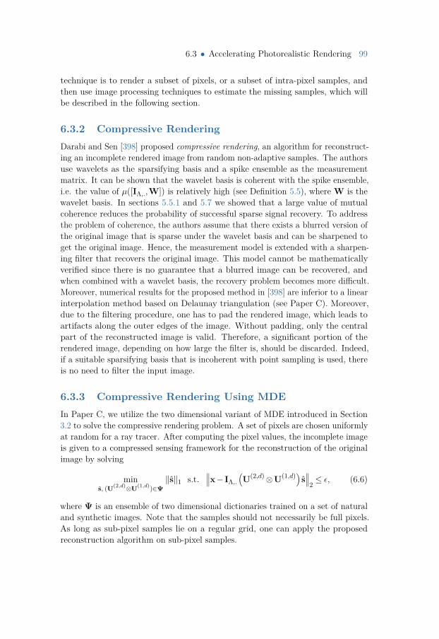
6.3 • Accelerating Photorealistic Rendering 99
technique is to render a subset of pixels, or a subset of intra-pixel samples, andthen use image processing techniques to estimate the missing samples, which willbe described in the following section.
6.3.2 Compressive RenderingDarabi and Sen [398] proposed compressive rendering, an algorithm for reconstruct-ing an incomplete rendered image from random non-adaptive samples. The authorsuse wavelets as the sparsifying basis and a spike ensemble as the measurementmatrix. It can be shown that the wavelet basis is coherent with the spike ensemble,i.e. the value of µ([IΛ,.,W]) is relatively high (see Definition 5.5), where W is thewavelet basis. In sections 5.5.1 and 5.7 we showed that a large value of mutualcoherence reduces the probability of successful sparse signal recovery. To addressthe problem of coherence, the authors assume that there exists a blurred version ofthe original image that is sparse under the wavelet basis and can be sharpened toget the original image. Hence, the measurement model is extended with a sharpen-ing filter that recovers the original image. This model cannot be mathematicallyverified since there is no guarantee that a blurred image can be recovered, andwhen combined with a wavelet basis, the recovery problem becomes more difficult.Moreover, numerical results for the proposed method in [398] are inferior to a linearinterpolation method based on Delaunay triangulation (see Paper C). Moreover,due to the filtering procedure, one has to pad the rendered image, which leads toartifacts along the outer edges of the image. Without padding, only the centralpart of the reconstructed image is valid. Therefore, a significant portion of therendered image, depending on how large the filter is, should be discarded. Indeed,if a suitable sparsifying basis that is incoherent with point sampling is used, thereis no need to filter the input image.
6.3.3 Compressive Rendering Using MDEIn Paper C, we utilize the two dimensional variant of MDE introduced in Section3.2 to solve the compressive rendering problem. A set of pixels are chosen uniformlyat random for a ray tracer. After computing the pixel values, the incomplete imageis given to a compressed sensing framework for the reconstruction of the originalimage by solving
mins, (U(2,d)⊗U(1,d))∈Ψ
‖s‖1 s.t.∥∥∥x− IΛ,.
(U(2,d)⊗U(1,d)) s
∥∥∥2≤ ε, (6.6)
where Ψ is an ensemble of two dimensional dictionaries trained on a set of naturaland synthetic images. Note that the samples should not necessarily be full pixels.As long as sub-pixel samples lie on a regular grid, one can apply the proposedreconstruction algorithm on sub-pixel samples.
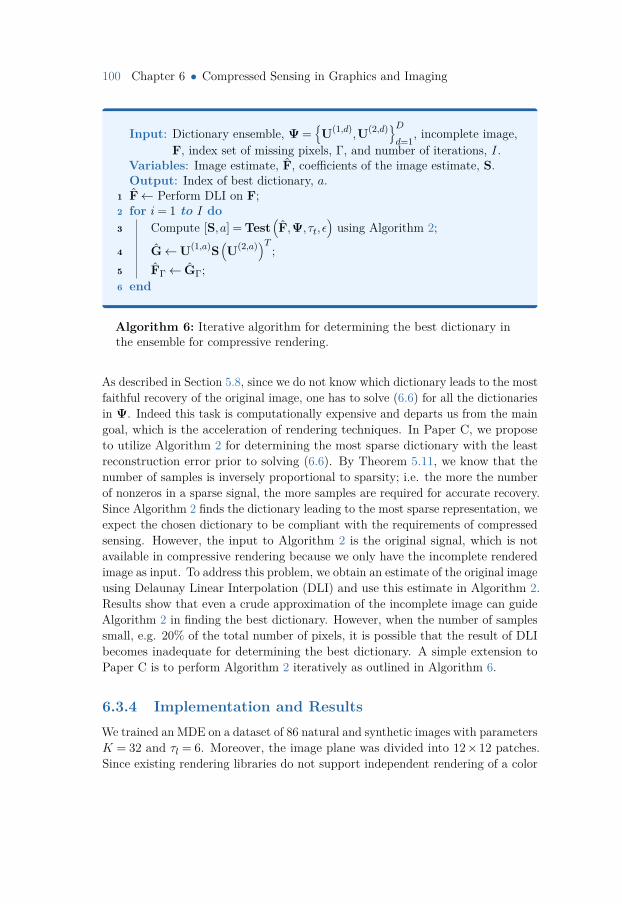
100 Chapter 6 • Compressed Sensing in Graphics and Imaging
Input: Dictionary ensemble, Ψ =U(1,d),U(2,d)D
d=1, incomplete image,
F, index set of missing pixels, Γ, and number of iterations, I.Variables: Image estimate, F, coefficients of the image estimate, S.Output: Index of best dictionary, a.
1 F← Perform DLI on F;2 for i= 1 to I do3 Compute [S,a] = Test
(F,Ψ, τt, ε
)using Algorithm 2;
4 G←U(1,a)S(U(2,a))T ;
5 FΓ← GΓ;6 end
Algorithm 6: Iterative algorithm for determining the best dictionary inthe ensemble for compressive rendering.
As described in Section 5.8, since we do not know which dictionary leads to the mostfaithful recovery of the original image, one has to solve (6.6) for all the dictionariesin Ψ. Indeed this task is computationally expensive and departs us from the maingoal, which is the acceleration of rendering techniques. In Paper C, we proposeto utilize Algorithm 2 for determining the most sparse dictionary with the leastreconstruction error prior to solving (6.6). By Theorem 5.11, we know that thenumber of samples is inversely proportional to sparsity; i.e. the more the numberof nonzeros in a sparse signal, the more samples are required for accurate recovery.Since Algorithm 2 finds the dictionary leading to the most sparse representation, weexpect the chosen dictionary to be compliant with the requirements of compressedsensing. However, the input to Algorithm 2 is the original signal, which is notavailable in compressive rendering because we only have the incomplete renderedimage as input. To address this problem, we obtain an estimate of the original imageusing Delaunay Linear Interpolation (DLI) and use this estimate in Algorithm 2.Results show that even a crude approximation of the incomplete image can guideAlgorithm 2 in finding the best dictionary. However, when the number of samplessmall, e.g. 20% of the total number of pixels, it is possible that the result of DLIbecomes inadequate for determining the best dictionary. A simple extension toPaper C is to perform Algorithm 2 iteratively as outlined in Algorithm 6.
6.3.4 Implementation and ResultsWe trained an MDE on a dataset of 86 natural and synthetic images with parametersK = 32 and τl = 6. Moreover, the image plane was divided into 12×12 patches.Since existing rendering libraries do not support independent rendering of a color
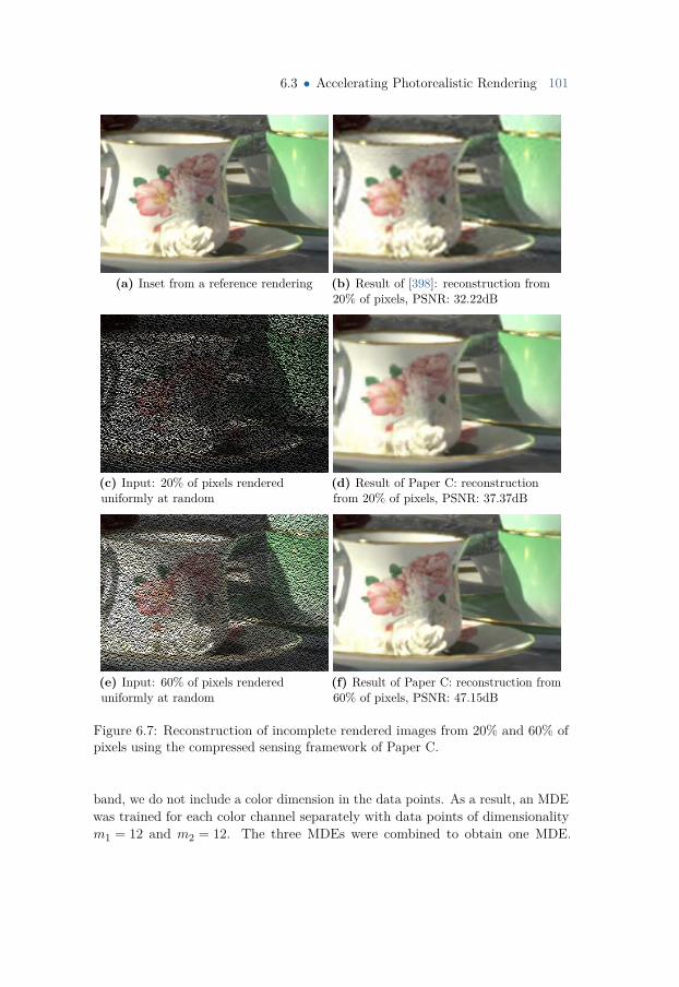
6.3 • Accelerating Photorealistic Rendering 101
(a) Inset from a reference rendering (b) Result of [398]: reconstruction from20% of pixels, PSNR: 32.22dB
(c) Input: 20% of pixels rendereduniformly at random
(d) Result of Paper C: reconstructionfrom 20% of pixels, PSNR: 37.37dB
(e) Input: 60% of pixels rendereduniformly at random
(f) Result of Paper C: reconstruction from60% of pixels, PSNR: 47.15dB
Figure 6.7: Reconstruction of incomplete rendered images from 20% and 60% ofpixels using the compressed sensing framework of Paper C.
band, we do not include a color dimension in the data points. As a result, an MDEwas trained for each color channel separately with data points of dimensionalitym1 = 12 and m2 = 12. The three MDEs were combined to obtain one MDE.
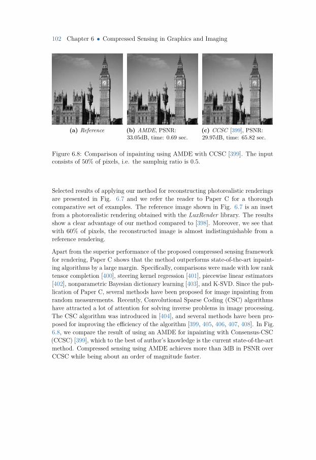
102 Chapter 6 • Compressed Sensing in Graphics and Imaging
(a) Reference (b) AMDE, PSNR:33.05dB, time: 0.69 sec.
(c) CCSC [399], PSNR:29.97dB, time: 65.82 sec.
Figure 6.8: Comparison of inpainting using AMDE with CCSC [399]. The inputconsists of 50% of pixels, i.e. the samplnig ratio is 0.5.
Selected results of applying our method for reconstructing photorealistic renderingsare presented in Fig. 6.7 and we refer the reader to Paper C for a thoroughcomparative set of examples. The reference image shown in Fig. 6.7 is an insetfrom a photorealistic rendering obtained with the LuxRender library. The resultsshow a clear advantage of our method compared to [398]. Moreover, we see thatwith 60% of pixels, the reconstructed image is almost indistinguishable from areference rendering.
Apart from the superior performance of the proposed compressed sensing frameworkfor rendering, Paper C shows that the method outperforms state-of-the-art inpaint-ing algorithms by a large margin. Specifically, comparisons were made with low ranktensor completion [400], steering kernel regression [401], piecewise linear estimators[402], nonparametric Bayesian dictionary learning [403], and K-SVD. Since the pub-lication of Paper C, several methods have been proposed for image inpainting fromrandom measurements. Recently, Convolutional Sparse Coding (CSC) algorithmshave attracted a lot of attention for solving inverse problems in image processing.The CSC algorithm was introduced in [404], and several methods have been pro-posed for improving the efficiency of the algorithm [399, 405, 406, 407, 408]. In Fig.6.8, we compare the result of using an AMDE for inpainting with Consensus-CSC(CCSC) [399], which to the best of author’s knowledge is the current state-of-the-artmethod. Compressed sensing using AMDE achieves more than 3dB in PSNR overCCSC while being about an order of magnitude faster.
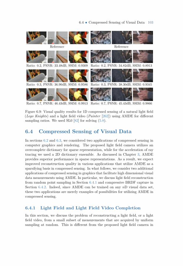
6.4 • Compressed Sensing of Visual Data 103
Reference Reference
Ratio: 0.2, PSNR: 33.48dB, SSIM: 0.9309 Ratio: 0.2, PSNR: 34.82dB, SSIM: 0.8913
Ratio: 0.3, PSNR: 36.90dB, SSIM: 0.9586 Ratio: 0.3, PSNR: 38.30dB, SSIM: 0.9345
Ratio: 0.7, PSNR: 46.43dB, SSIM: 0.9913 Ratio: 0.7, PSNR: 45.43dB, SSIM: 0.9866
Figure 6.9: Visual quality results for 1D compressed sensing of a natural light field(Lego Knights) and a light field video (Painter [262]) using AMDE for differentsampling ratios. We used SL0 [82] for solving (5.8).
6.4 Compressed Sensing of Visual DataIn sections 6.2 and 6.3, we considered two applications of compressed sensing incomputer graphics and rendering. The proposed light field camera utilizes anovercomplete dictionary for sparse representation, while for the acceleration of raytracing we used a 2D dictionary ensemble. As discussed in Chapter 3, AMDEprovides superior performance in sparse representations. As a result, we expectimproved reconstruction quality in various applications that utilize AMDE as asparsifying basis in compressed sensing. In what follows, we consider two additionalapplications of compressed sensing in graphics that facilitate high dimensional visualdata measurements using AMDE. In particular, we discuss light field reconstructionfrom random point sampling in Section 6.4.1 and compressive BRDF capture inSection 6.4.2. Indeed, since AMDE can be trained on any nD visual data set,these two applications are merely examples of possibilities for utilizing AMDE incompressed sensing.
6.4.1 Light Field and Light Field Video CompletionIn this section, we discuss the problem of reconstructing a light field, or a lightfield video, from a small subset of measurements that are acquired by uniformsampling at random. This is different from the proposed light field camera in
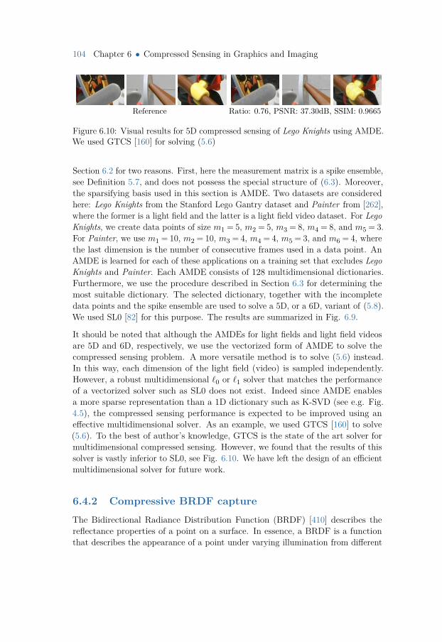
104 Chapter 6 • Compressed Sensing in Graphics and Imaging
Reference Ratio: 0.76, PSNR: 37.30dB, SSIM: 0.9665
Figure 6.10: Visual results for 5D compressed sensing of Lego Knights using AMDE.We used GTCS [160] for solving (5.6)
Section 6.2 for two reasons. First, here the measurement matrix is a spike ensemble,see Definition 5.7, and does not possess the special structure of (6.3). Moreover,the sparsifying basis used in this section is AMDE. Two datasets are consideredhere: Lego Knights from the Stanford Lego Gantry dataset and Painter from [262],where the former is a light field and the latter is a light field video dataset. For LegoKnights, we create data points of size m1 = 5, m2 = 5, m3 = 8, m4 = 8, and m5 = 3.For Painter, we use m1 = 10, m2 = 10, m3 = 4, m4 = 4, m5 = 3, and m6 = 4, wherethe last dimension is the number of consecutive frames used in a data point. AnAMDE is learned for each of these applications on a training set that excludes LegoKnights and Painter. Each AMDE consists of 128 multidimensional dictionaries.Furthermore, we use the procedure described in Section 6.3 for determining themost suitable dictionary. The selected dictionary, together with the incompletedata points and the spike ensemble are used to solve a 5D, or a 6D, variant of (5.8).We used SL0 [82] for this purpose. The results are summarized in Fig. 6.9.
It should be noted that although the AMDEs for light fields and light field videosare 5D and 6D, respectively, we use the vectorized form of AMDE to solve thecompressed sensing problem. A more versatile method is to solve (5.6) instead.In this way, each dimension of the light field (video) is sampled independently.However, a robust multidimensional `0 or `1 solver that matches the performanceof a vectorized solver such as SL0 does not exist. Indeed since AMDE enablesa more sparse representation than a 1D dictionary such as K-SVD (see e.g. Fig.4.5), the compressed sensing performance is expected to be improved using aneffective multidimensional solver. As an example, we used GTCS [160] to solve(5.6). To the best of author’s knowledge, GTCS is the state of the art solver formultidimensional compressed sensing. However, we found that the results of thissolver is vastly inferior to SL0, see Fig. 6.10. We have left the design of an efficientmultidimensional solver for future work.
6.4.2 Compressive BRDF capture
The Bidirectional Radiance Distribution Function (BRDF) [410] describes thereflectance properties of a point on a surface. In essence, a BRDF is a functionthat describes the appearance of a point under varying illumination from different
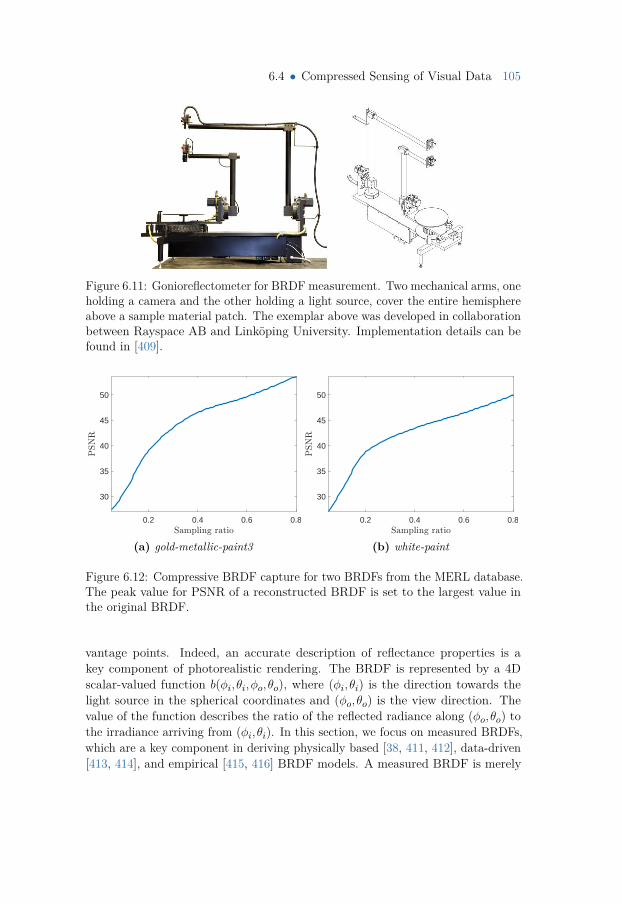
6.4 • Compressed Sensing of Visual Data 105
Figure 6.11: Gonioreflectometer for BRDF measurement. Two mechanical arms, oneholding a camera and the other holding a light source, cover the entire hemisphereabove a sample material patch. The exemplar above was developed in collaborationbetween Rayspace AB and Linköping University. Implementation details can befound in [409].
0.2 0.4 0.6 0.8
30
35
40
45
50
(a) gold-metallic-paint3
0.2 0.4 0.6 0.8
30
35
40
45
50
(b) white-paint
Figure 6.12: Compressive BRDF capture for two BRDFs from the MERL database.The peak value for PSNR of a reconstructed BRDF is set to the largest value inthe original BRDF.
vantage points. Indeed, an accurate description of reflectance properties is akey component of photorealistic rendering. The BRDF is represented by a 4Dscalar-valued function b(φi, θi,φo, θo), where (φi, θi) is the direction towards thelight source in the spherical coordinates and (φo, θo) is the view direction. Thevalue of the function describes the ratio of the reflected radiance along (φo, θo) tothe irradiance arriving from (φi, θi). In this section, we focus on measured BRDFs,which are a key component in deriving physically based [38, 411, 412], data-driven[413, 414], and empirical [415, 416] BRDF models. A measured BRDF is merely
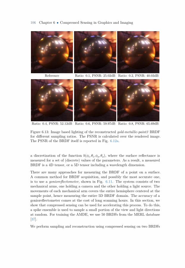
106 Chapter 6 • Compressed Sensing in Graphics and Imaging
Reference Ratio: 0.1, PSNR: 25.02dB Ratio: 0.2, PSNR: 40.03dB
Ratio: 0.4, PSNR: 52.12dB Ratio: 0.6, PSNR: 59.97dB Ratio: 0.8, PSNR: 65.69dB
Figure 6.13: Image based lighting of the reconstructed gold-metallic-paint3 BRDFfor different sampling ratios. The PSNR is calculated over the rendered image.The PSNR of the BRDF itself is reported in Fig. 6.12a.
a discretization of the function b(φi, θi,φo, θo), where the surface reflectance ismeasured for a set of (discrete) values of the parameters. As a result, a measuredBRDF is a 4D tensor, or a 5D tensor including a wavelength dimension.
There are many approaches for measuring the BRDF of a point on a surface.A common method for BRDF acquisition, and possibly the most accurate one,is to use a gonioreflectometer, shown in Fig. 6.11. The system consists of twomechanical arms, one holding a camera and the other holding a light source. Themovements of each mechanical arm covers the entire hemisphere centered at thesample point, hence measuring the entire 5D BRDF domain. The accuracy of agonioreflectometer comes at the cost of long scanning hours. In this section, weshow that compressed sensing can be used for accelerating this process. To do this,a spike ensemble is used to sample a small portion of the view and light directionsat random. For training the AMDE, we use 50 BRDFs from the MERL database[37].
We perform sampling and reconstruction using compressed sensing on two BRDFs
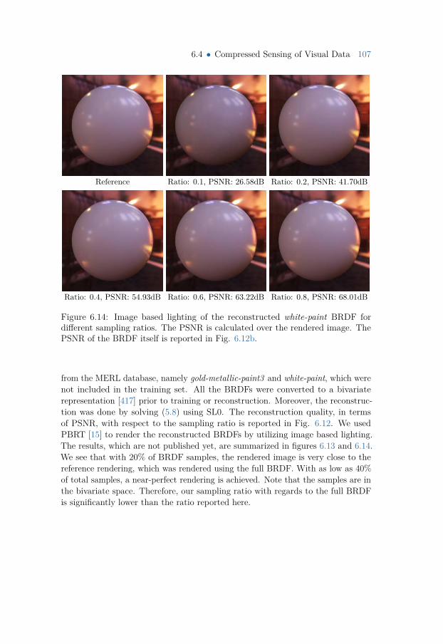
6.4 • Compressed Sensing of Visual Data 107
Reference Ratio: 0.1, PSNR: 26.58dB Ratio: 0.2, PSNR: 41.70dB
Ratio: 0.4, PSNR: 54.93dB Ratio: 0.6, PSNR: 63.22dB Ratio: 0.8, PSNR: 68.01dB
Figure 6.14: Image based lighting of the reconstructed white-paint BRDF fordifferent sampling ratios. The PSNR is calculated over the rendered image. ThePSNR of the BRDF itself is reported in Fig. 6.12b.
from the MERL database, namely gold-metallic-paint3 and white-paint, which werenot included in the training set. All the BRDFs were converted to a bivariaterepresentation [417] prior to training or reconstruction. Moreover, the reconstruc-tion was done by solving (5.8) using SL0. The reconstruction quality, in termsof PSNR, with respect to the sampling ratio is reported in Fig. 6.12. We usedPBRT [15] to render the reconstructed BRDFs by utilizing image based lighting.The results, which are not published yet, are summarized in figures 6.13 and 6.14.We see that with 20% of BRDF samples, the rendered image is very close to thereference rendering, which was rendered using the full BRDF. With as low as 40%of total samples, a near-perfect rendering is achieved. Note that the samples are inthe bivariate space. Therefore, our sampling ratio with regards to the full BRDFis significantly lower than the ratio reported here.
108 Chapter 6 • Compressed Sensing in Graphics and Imaging
6.5 Summary and Future Work
In this chapter, we presented three applications in computer graphics and imageprocessing that utilize the rich theoretical foundation of compressed sensing. First,a light field camera design was proposed that is simple to implement, yet providesgreat flexibility to capture high quality light fields without the requirement ofmultiple sensors. The simulation results of the proposed method show significantimprovements over previous work. Equation (6.3) shows that the measurementmatrix for a single-sensor compressive light field camera possesses certain structuresand is not fully random. An exciting venue for research is to compute metricsfor exact recovery such as mutual coherence, RIC, and ERC for the measurementmatrix in (6.3). The author believes that it is possible to derive analytical formulasfor a collection of recovery metrics given the structure present in the sensing matrix.In this way, one can use a rich collection of existing theoretical results for recoveryconditions based on the aforementioned metrics.
The compressed sensing framework used for the light field camera is based on avariant of K-SVD [164], hence the light field is assumed to be a 1D signal. Giventhe superior results of the AMDE in compression, which is achieved by increasingsparsity, we expect improvements in the results of the light field camera witha multidimensional compressed sensing framework based on the AMDE. Sincemultidimensional sparse recovery algorithms have not matured yet, we have leftthe design of a multidimensional light field camera for future work. Indeed suchan approach can offer important improvements. For instance, it is known that alight field exhibits different patterns of sparsity along its various dimensions. Alight field may be sparse along its angular dimension but dense along the spatialdimension, or vice versa. As a result, it is beneficial to dedicate more samples alongdimensions that are less sparse. This is only possible when a multidimensionalcompressed sensing is used (i.e. equation (5.6)).
The proposed light field camera in Section 6.2 can be extended for capturing HighDynamic Range (HDR) light fields and light field videos. There exists single-shot, single-sensor HDR imaging systems [418, 419, 420], where an HDR imageis reconstructed from two horizontal interlaced ISO settings over the sensor (alsoknown as dual-ISO HDR imaging). Such a reconstruction procedure can indeedbe formulated using compressed sensing. Therefore, it is possible to combinethe reconstruction of a dual-ISO HDR image and the measurement model of theproposed light field camera in (6.3); hence, achieving a single-shot HDR light fieldimaging system.
An interesting direction for future research is the utilization of Theorem 5.11 forguiding the design of compressive light field cameras that utilize an ensemble ofdictionaries. Theorem 5.11 shows that the maximum row-norm of the equivalent

6.5 • Summary and Future Work 109
measurement matrix should be as small as possible. This requirement is equivalentto having an equivalent measurement matrix with relatively uniform values forrow norms (assuming that the columns of the equivalent measurement matrixare normalized). There are two important factors that determine the equivalentmeasurement matrix. First, the design of the light field camera directly affects thestructure of the measurement matrix. For instance, by changing the placementof the mask, one obtains a different measurement matrix. Second, the type ofthe dictionaries in the ensemble also affects the equivalent measurement matrix.Indeed if we know the properties of a “good” measurement matrix, as defined inTheorem 5.11, hardware implementations can be more cost effective and efficient.The theoretical analysis of existing light field capture systems using Theorem 5.11is also left for future work. Of particular interest to the author is the design ofan ensemble of nD overcomplete dictionaries and separable sensing operators thatconform to the requirements of Theorem 5.11.
We discussed a method for accelerating the photorealistic rendering techniques. Theproposed approach is based on rendering a subset of pixels and using a compressedsensing framework to reconstruct the remaining pixels. A sampling ratio of 60%shows production quality results using the proposed framework. Moreover, at aratio of 20%, an acceptable image quality is achieved. An advantage of this methodis that it can be applied to any ray tracing technique since we only consider imageplane samples. Extension of the proposed compressive rendering to the full raytracing pipeline is left for future work. In other words, it is possible to evaluatethe reflection equation at each bounce using compressed sensing. We believe thatthis approach is feasible since several building blocks has already been discussed inthis thesis. For instance, BRDFs are known to be very sparse objects in a suitablebasis. Moreover, the reflectance equation at a point is expressed by the convolutionof incoming radiance with the BRDF [45]. Since a convolution can be written as amatrix/vector multiplication, we can apply compressed sensing to determine theoutgoing radiance.
In Chapter 3, we showed (empirically) that the ensemble of multidimensional dictio-naries promotes sparsity. Hence, the author is interested in exploring and designingnew approaches for efficient utilization of dictionaries ensembles for compressedsensing. Given that multidimensional compressed sensing and multidimensionalovercomplete dictionary learning are unsolved problems, we believe that thereexists several new research directions. Note that AMDE, introduced in Section3.3, is an ensemble of multidimensional orthonormal dictionaries. Therefore, weexpect significant improvements in compressed sensing performance for an ensembleof overcomplete multidimensional dictionaries. This is due to the fact that anovercomplete dictionary, compared to an orthonormal one, can produce sparserepresentations for a larger set of signals.

Ch
ap
te
r
7Concluding Remarks and Outlook
In this thesis, we presented methods for compression and compressed sensing ofvisual data. The foundation of these methods is sparse signal representation. In aninteresting article, M. Elad [421] presents the progression of sparse representationtechniques since the inception of the field, as well as dividing the future work intothree major directions:
1. Theoretical frontiers: Improving existing theoretical guarantees in com-pressed sensing to better match empirical results.
2. Model improvements: Establishing new dictionary learning techniquesthat promote sparsity, while reducing the representation error.
3. Applications: Apply sparse representation and compressed sensing tech-niques to improve the quality, as well as efficiency, of compression andsampling (capturing) of visual data.
This thesis makes a number of contributions in all the three areas mentioned above.In what follows, we will summarize these contributions and state several unansweredresearch questions that can further push the boundaries of sparse representationtechniques for visual data in the near future.
112 Chapter 7 • Concluding Remarks and Outlook
7.1 Theoretical FrontiersThis thesis presented two key contributions on advancing the theoretical frontiersof sparse representations and compressed sensing. First, we presented exactrecovery conditions of the OMP algorithm for sparse signals contaminated withwhite Gaussian noise. The lower bound on the probability of success for OMPincludes important (and easily computable) signal parameters, as well as dictionaryproperties. Additionally, we combined an upper bound on the representation errorwith the lower bound on the probability of success to derive new bounds that showthe effect of signal parameters on the performance of OMP. Second, we deriveduniqueness conditions for exact recovery of multidimensional sparse signals under anensemble of multidimensional dictionaries (e.g. AMDE). This novel analysis showsthe required conditions for a suitable multidimensional ensemble of dictionaries thatenables efficient compressed sensing. Moreover, we derived the required numberof samples and sparsity of signals, which are crucial in designing state of the artmeasurement techniques for visual data including light field cameras, as well asBRDF and BTF measurements devices. The author of this thesis believes that theresults presented here have posed many new questions that can be subjects forfuture research. For instance,
• Theorem 5.8 was shown to significantly improve the previous results usingmutual coherence for the recovery conditions of OMP. However, there is stilla large gap between the theoretical and empirical results. Can the analysis beimproved to have a better match between empirical and theoretical results?
• There exists multidimensional variants of OMP [102]. Can we extend theanalysis in Paper F to accommodate these techniques?
• Theorem 5.11 presented theoretical guarantees for an ensemble of multidi-mensional dictionaries in a vectorized formulation, i.e. (5.46). Can we derivetheoretical guarantees for an ensemble of multidimensional dictionaries in thenative nD formulation (i.e. (5.59))?
• Using the theoretical results presented in this thesis, can we derive newperformance guarantees for existing capturing mechanism of visual data suchas BRDFs and BTFs?
• Can we derive optimal sensing matrices (according to various metrics incompressed sensing) that enable efficient BRDF capturing with the minimalnumber of samples?
• Can we derive closed form formulas for mutual coherence, RIP, or ERC ofthe single sensor light field camera with a color coded mask? And from that,
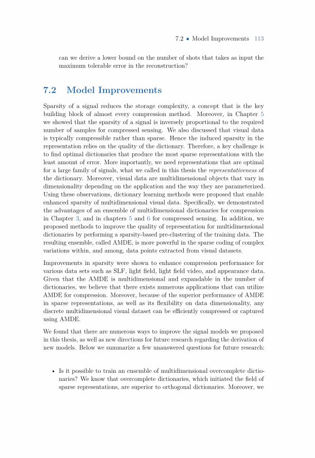
7.2 • Model Improvements 113
can we derive a lower bound on the number of shots that takes as input themaximum tolerable error in the reconstruction?
7.2 Model ImprovementsSparsity of a signal reduces the storage complexity, a concept that is the keybuilding block of almost every compression method. Moreover, in Chapter 5we showed that the sparsity of a signal is inversely proportional to the requirednumber of samples for compressed sensing. We also discussed that visual datais typically compressible rather than sparse. Hence the induced sparsity in therepresentation relies on the quality of the dictionary. Therefore, a key challenge isto find optimal dictionaries that produce the most sparse representations with theleast amount of error. More importantly, we need representations that are optimalfor a large family of signals, what we called in this thesis the representativeness ofthe dictionary. Moreover, visual data are multidimensional objects that vary indimensionality depending on the application and the way they are parameterized.Using these observations, dictionary learning methods were proposed that enableenhanced sparsity of multidimensional visual data. Specifically, we demonstratedthe advantages of an ensemble of multidimensional dictionaries for compressionin Chapter 3, and in chapters 5 and 6 for compressed sensing. In addition, weproposed methods to improve the quality of representation for multidimensionaldictionaries by performing a sparsity-based pre-clustering of the training data. Theresulting ensemble, called AMDE, is more powerful in the sparse coding of complexvariations within, and among, data points extracted from visual datasets.
Improvements in sparsity were shown to enhance compression performance forvarious data sets such as SLF, light field, light field video, and appearance data.Given that the AMDE is multidimensional and expandable in the number ofdictionaries, we believe that there exists numerous applications that can utilizeAMDE for compression. Moreover, because of the superior performance of AMDEin sparse representations, as well as its flexibility on data dimensionality, anydiscrete multidimensional visual dataset can be efficiently compressed or capturedusing AMDE.
We found that there are numerous ways to improve the signal models we proposedin this thesis, as well as new directions for future research regarding the derivation ofnew models. Below we summarize a few unanswered questions for future research:
• Is it possible to train an ensemble of multidimensional overcomplete dictio-naries? We know that overcomplete dictionaries, which initiated the field ofsparse representations, are superior to orthogonal dictionaries. Moreover, we

114 Chapter 7 • Concluding Remarks and Outlook
showed in Chapter 3 that an ensemble of multidimensional orthogonal dictio-naries is superior to a single overcomplete dictionary. Therefore, it is expected(by intuition) that an ensemble of multidimensional overcomplete dictionarieswill significantly improve the signal model for sparse representation.
• The AMDE is trained by applying pre-clustering to the training data points,followed by ensemble training for each pre-cluster. Indeed an iterative ap-proach can improve the quality of AMDE for sparse representation. It is leftto be seen how much this can improve the performance of AMDE.
• Inspired by wavelets, can we derive a training method that iteratively appliespre-clustering and dictionary training in a multi-level fashion?
• Can we find methods for automatic tuning of the number of pre-clustersand dictionaries? This is indeed an open problem in most clustering anddictionary training algorithms.
7.3 ApplicationsWe considered several applications for utilizing sparse representations of visualdata in compression and compressed sensing. For compression, we used a variantof MDE for precomputed photorealistic rendering without any limitations on thecomplexity of materials or light sources. We also showed that AMDE is significantlysuperior to previous methods in compression of light field and light field videodatasets. Moreover, we demonstrated that AMDE enables real time playbackof high-resolution light field videos. To show the flexibility of AMDE, we alsopresented the compression of large-scale appearance data captured using a rotatingcamera rig. For compressed sensing, a design of a light field camera with a singlesensor and a color coded mask was proposed which enables fast, high quality,and cheap light field capture. Moreover, we used ensemble of 2D dictionaries toaccelerate photorealistic rendering techniques. And finally, we demonstrated thatthe ensemble of multidimensional dictionaries can be used for compressed sensingof a variety of datasets including light fields, light field videos, and BRDFs.
The possibilities of utilizing the proposed methods, and in general sparse represen-tations, in computer graphics, imaging, and visualization are, figuratively, endless.There are only a few works on sparse representations and compressed sensing incomputer graphics. Hence there exists numerous directions for future work, both bythe extension of the methods discussed in this thesis, as well as their applicationsin new areas of computer graphics. For instance,
• We only discussed selected applications in computer graphics for compressionand compressed sensing of visual data. Utilizing AMDE for compression of
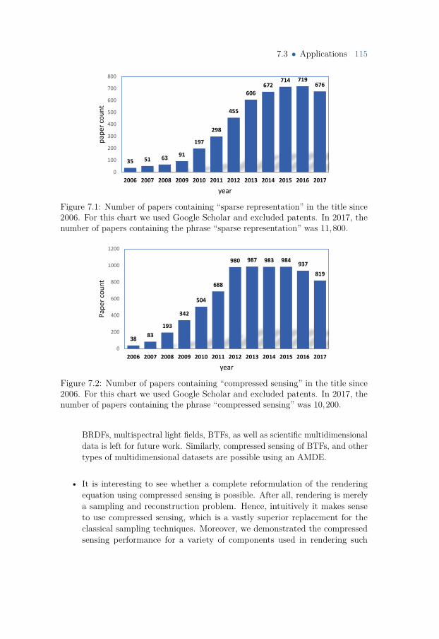
7.3 • Applications 115
35 51 6391
197
298
455
606672
714 719676
0
100
200
300
400
500
600
700
800
2006 2007 2008 2009 2010 2011 2012 2013 2014 2015 2016 2017
pap
er c
ou
nt
year
Figure 7.1: Number of papers containing “sparse representation” in the title since2006. For this chart we used Google Scholar and excluded patents. In 2017, thenumber of papers containing the phrase “sparse representation” was 11,800.
3883
193
342
504
688
980 987 983 984937
819
0
200
400
600
800
1000
1200
2006 2007 2008 2009 2010 2011 2012 2013 2014 2015 2016 2017
Pap
er c
ou
nt
year
Figure 7.2: Number of papers containing “compressed sensing” in the title since2006. For this chart we used Google Scholar and excluded patents. In 2017, thenumber of papers containing the phrase “compressed sensing” was 10,200.
BRDFs, multispectral light fields, BTFs, as well as scientific multidimensionaldata is left for future work. Similarly, compressed sensing of BTFs, and othertypes of multidimensional datasets are possible using an AMDE.
• It is interesting to see whether a complete reformulation of the renderingequation using compressed sensing is possible. After all, rendering is merelya sampling and reconstruction problem. Hence, intuitively it makes senseto use compressed sensing, which is a vastly superior replacement for theclassical sampling techniques. Moreover, we demonstrated the compressedsensing performance for a variety of components used in rendering such
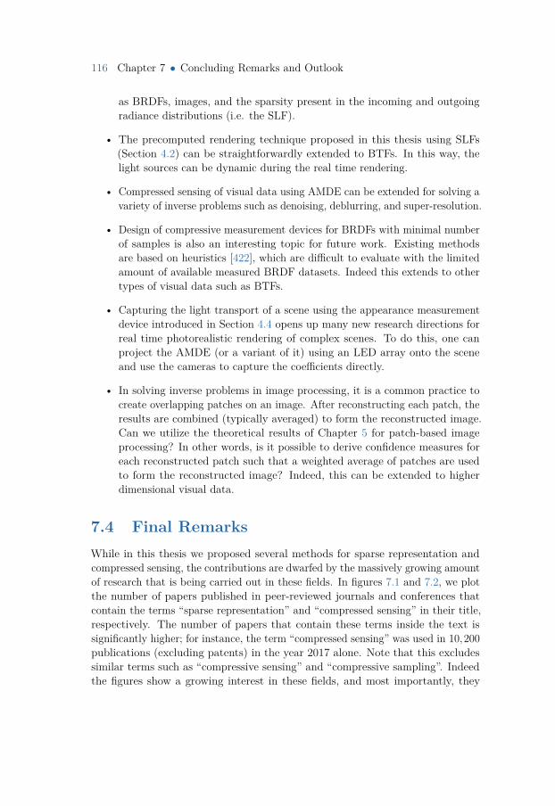
116 Chapter 7 • Concluding Remarks and Outlook
as BRDFs, images, and the sparsity present in the incoming and outgoingradiance distributions (i.e. the SLF).
• The precomputed rendering technique proposed in this thesis using SLFs(Section 4.2) can be straightforwardly extended to BTFs. In this way, thelight sources can be dynamic during the real time rendering.
• Compressed sensing of visual data using AMDE can be extended for solving avariety of inverse problems such as denoising, deblurring, and super-resolution.
• Design of compressive measurement devices for BRDFs with minimal numberof samples is also an interesting topic for future work. Existing methodsare based on heuristics [422], which are difficult to evaluate with the limitedamount of available measured BRDF datasets. Indeed this extends to othertypes of visual data such as BTFs.
• Capturing the light transport of a scene using the appearance measurementdevice introduced in Section 4.4 opens up many new research directions forreal time photorealistic rendering of complex scenes. To do this, one canproject the AMDE (or a variant of it) using an LED array onto the sceneand use the cameras to capture the coefficients directly.
• In solving inverse problems in image processing, it is a common practice tocreate overlapping patches on an image. After reconstructing each patch, theresults are combined (typically averaged) to form the reconstructed image.Can we utilize the theoretical results of Chapter 5 for patch-based imageprocessing? In other words, is it possible to derive confidence measures foreach reconstructed patch such that a weighted average of patches are usedto form the reconstructed image? Indeed, this can be extended to higherdimensional visual data.
7.4 Final RemarksWhile in this thesis we proposed several methods for sparse representation andcompressed sensing, the contributions are dwarfed by the massively growing amountof research that is being carried out in these fields. In figures 7.1 and 7.2, we plotthe number of papers published in peer-reviewed journals and conferences thatcontain the terms “sparse representation” and “compressed sensing” in their title,respectively. The number of papers that contain these terms inside the text issignificantly higher; for instance, the term “compressed sensing” was used in 10,200publications (excluding patents) in the year 2017 alone. Note that this excludessimilar terms such as “compressive sensing” and “compressive sampling”. Indeedthe figures show a growing interest in these fields, and most importantly, they

7.4 • Final Remarks 117
show an increasing number of research questions year by year. This thesis is noexception in this trend and we have presented more questions for future work thanthe questions we hopefully have answered by the contributions of this thesis. Theauthor of this thesis finds the growing amount of opportunities in these fields, andespecially their applications in computer graphics, to be extremely exciting.

Bibliography
[1] E. Miandji, S. Hajisharif, and J. Unger, “A Unified Framework for Compres-sion and Compressed Sensing of Light Fields and Light Field Videos,” ACMTransactions on Graphics, Provisionally accepted.
[2] E. Miandji, J. Unger, and C. Guillemot, “Multi-Shot Single Sensor Light FieldCamera Using a Color Coded Mask,” in 26th European Signal ProcessingConference (EUSIPCO) 2018. IEEE, Sept 2018.
[3] E. Miandji†, M. Emadi†, and J. Unger, “OMP-based DOA Estimation Per-formance Analysis,” Digital Signal Processing, vol. 79, pp. 57–65, Aug 2018,† equal contributor.
[4] E. Miandji†, M. Emadi†, J. Unger, and E. Afshari, “On Probability ofSupport Recovery for Orthogonal Matching Pursuit Using Mutual Coherence,”IEEE Signal Processing Letters, vol. 24, no. 11, pp. 1646–1650, Nov 2017,† equal contributor.
[5] E. Miandji and J. Unger, “On Nonlocal Image Completion Using an Ensembleof Dictionaries,” in 2016 IEEE International Conference on Image Processing(ICIP). IEEE, Sept 2016, pp. 2519–2523.
[6] E. Miandji, J. Kronander, and J. Unger, “Compressive Image Reconstructionin Reduced Union of Subspaces,” Computer Graphics Forum, vol. 34, no. 2,pp. 33–44, May 2015.
[7] E. Miandji, J. Kronander, and J. Unger, “Learning Based Compression ofSurface Light Fields for Real-time Rendering of Global Illumination Scenes,”in SIGGRAPH Asia 2013 Technical Briefs. ACM, 2013, pp. 24:1–24:4.
[8] G. Baravdish, E. Miandji, and J. Unger, “GPU Accelerated Sparse Repre-sentation of Light Fields,” in 14th International Conference on ComputerVision Theory and Applications (VISAPP 2019), submitted. [page 57]
[9] E. Miandji†, M. Emadi†, and J. Unger, “A Performance Guarantee for Or-thogonal Matching Pursuit Using Mutual Coherence,” Circuits, Systems, andSignal Processing, vol. 37, no. 4, pp. 1562–1574, Apr 2018, † equal contributor.
120 Bibliography
[10] J. Kronander, F. Banterle, A. Gardner, E. Miandji, and J. Unger, “Photo-realistic Rendering of Mixed Reality Scenes,” Computer Graphics Forum,vol. 34, no. 2, pp. 643–665, May 2015.
[11] S. Mohseni, N. Zarei, E. Miandji, and G. Ardeshir, “Facial Expression Recog-nition Using Facial Graph,” in Workshop on Face and Facial ExpressionRecognition from Real World Videos (ICPR 2014). Cham: Springer Interna-tional Publishing, 2014, pp. 58–66.
[12] S. Hajisharif, J. Kronander, E. Miandji, and J. Unger, “Real-time ImageBased Lighting with Streaming HDR-light Probe Sequences,” in SIGRAD2012: Interactive Visual Analysis of Data. Linköping University ElectronicPress, Nov 2012.
[13] E. Miandji, J. Kronander, and J. Unger, “Geometry Independent SurfaceLight Fields for Real Time Rendering of Precomputed Global Illumination,”in SIGRAD 2011. Linköping University Electronic Press, 2011.
[14] E. Miandji, M. H. Sargazi Moghadam, F. F. Samavati, and M. Emadi, “Real-time Multi-band Synthesis of Ocean Water With New Iterative Up-samplingTechnique,” The Visual Computer, vol. 25, no. 5, pp. 697–705, May 2009.[page 47]
[15] M. Pharr and G. Humphreys, Physically Based Rendering, Second Edition:From Theory To Implementation, 2nd ed. San Francisco, CA, USA: MorganKaufmann Publishers Inc., 2010. [pages xiii, 51, and 107]
[16] S. Lloyd, “Least squares quantization in PCM,” IEEE Transactions onInformation Theory, vol. 28, no. 2, pp. 129–137, 1982. [pages xiii and 39]
[17] K. Marwah, G. Wetzstein, Y. Bando, and R. Raskar, “Compressive Light FieldPhotography Using Overcomplete Dictionaries and Optimized Projections,”ACM Transactions on Graphics, vol. 32, no. 4, pp. 46:1–46:12, July 2013.[pages xv, 10, 93, 94, and 95]
[18] Z. Ben-Haim, Y. C. Eldar, and M. Elad, “Coherence-Based PerformanceGuarantees for Estimating a Sparse Vector Under Random Noise,” IEEETransactions on Signal Processing, vol. 58, no. 10, pp. 5030–5043, Oct 2010.[pages xv, 74, 75, and 76]
[19] T. Hey, S. Tansley, and K. Tolle, The Fourth Paradigm: Data-IntensiveScientific Discovery. Microsoft Research, Oct 2009. [page 1]
[20] S. J. Gortler, R. Grzeszczuk, R. Szeliski, and M. F. Cohen, “The Lumigraph,”in Proceedings of the 23rd Annual Conference on Computer Graphics and
Bibliography 121
Interactive Techniques, ser. SIGGRAPH ’96. New York, NY, USA: ACM,Aug 1996, pp. 43–54. [pages 1 and 27]
[21] B. S. Wilburn, M. Smulski, H.-H. K. Lee, and M. A. Horowitz, “Light fieldvideo camera,” pp. 4674 – 4674 – 8, 2001. [page 1]
[22] G. D., G. G.C., G. A., D. C., and G. M., “BRDF Representation andAcquisition,” Computer Graphics Forum, vol. 35, no. 2, pp. 625–650, May2016. [page 1]
[23] Z. Zhou, G. Chen, Y. Dong, D. Wipf, Y. Yu, J. Snyder, and X. Tong, “Sparse-as-possible SVBRDF Acquisition,” ACM Transactions on Graphics, vol. 35,no. 6, pp. 189:1–189:12, Nov 2016. [page 1]
[24] G. R. Arce, D. J. Brady, L. Carin, H. Arguello, and D. S. Kittle, “CompressiveCoded Aperture Spectral Imaging: An Introduction,” IEEE Signal ProcessingMagazine, vol. 31, no. 1, pp. 105–115, Jan 2014. [page 1]
[25] K. J. Dana, B. van Ginneken, S. K. Nayar, and J. J. Koenderink, “Reflectanceand Texture of Real-world Surfaces,” ACM Transactions on Graphics, vol. 18,no. 1, pp. 1–34, Jan 1999. [page 1]
[26] M. Lustig, D. Donoho, and J. M. Pauly, “Sparse MRI: The Applicationof Compressed Sensing for Rapid MR Imaging,” Magnetic Resonance inMedicine, vol. 58, no. 6, pp. 1182–1195, Oct 2007. [pages 1, 10, and 90]
[27] G. Wetzstein, D. Lanman, M. Hirsch, W. Heidrich, and R. Raskar, “Com-pressive Light Field Displays,” IEEE Computer Graphics and Applications,vol. 32, no. 5, pp. 6–11, Sept 2012. [page 2]
[28] G. Wetzstein, D. Lanman, M. Hirsch, and R. Raskar, “Tensor Displays:Compressive Light Field Synthesis Using Multilayer Displays with DirectionalBacklighting,” ACM Transactions on Graphics, vol. 31, no. 4, pp. 80:1–80:11,Jul 2012. [pages 2 and 32]
[29] S. Lee, C. Jang, S. Moon, J. Cho, and B. Lee, “Additive Light Field Displays:Realization of Augmented Reality with Holographic Optical Elements,” ACMTransactions on Graphics, vol. 35, no. 4, pp. 60:1–60:13, Jul 2016. [page 2]
[30] B. Koniaris, M. Kosek, D. Sinclair, and K. Mitchell, “Real-time Render-ing with Compressed Animated Light Fields,” in Proceedings of the 43rdGraphics Interface Conference, ser. GI ’17. Canadian Human-ComputerCommunications Society, 2017, pp. 33–40. [page 2]
[31] W.-C. Chen, J.-Y. Bouguet, M. H. Chu, and R. Grzeszczuk, “Light FieldMapping: Efficient Representation and Hardware Rendering of Surface Light
122 Bibliography
Fields,” ACM Transactions on Graphics, vol. 21, no. 3, pp. 447–456, Jul 2002.[pages 2 and 47]
[32] D. Antensteiner and S. Stolc, “Full BRDF Reconstruction Using CNNs fromPartial Photometric Stereo-Light Field Data,” in 2017 IEEE Conference onComputer Vision and Pattern Recognition Workshops, 2017, pp. 1726–1734.[page 2]
[33] R. Ramamoorthi, M. Koudelka, and P. Belhumeur, “A Fourier theory for castshadows,” IEEE Transactions on Pattern Analysis and Machine Intelligence,vol. 27, no. 2, pp. 288–295, Feb 2005. [page 2]
[34] Y.-T. Tsai, “Multiway K-Clustered Tensor Approximation: Toward High-Performance Photorealistic Data-Driven Rendering,” ACM Transactions onGraphics, vol. 34, no. 5, pp. 157:1–157:15, Nov 2015. [pages 2, 32, and 34]
[35] X. Sun, Q. Hou, Z. Ren, K. Zhou, and B. Guo, “Radiance Transfer Biclusteringfor Real-Time All-Frequency Biscale Rendering,” IEEE Transactions onVisualization and Computer Graphics, vol. 17, no. 1, pp. 64–73, Jan 2011.[page 2]
[36] G. Müller, G. H. Bendels, and R. Klein, “Rapid Synchronous Acquisition ofGeometry and Appearance of Cultural Heritage Artefacts,” in Proceedingsof the 6th International Conference on Virtual Reality, Archaeology andIntelligent Cultural Heritage, ser. VAST’05. Eurographics Association, 2005,pp. 13–20. [page 2]
[37] W. Matusik, H. Pfister, M. Brand, and L. McMillan, “A Data-driven Re-flectance Model,” ACM Transactions on Graphics, vol. 22, no. 3, pp. 759–769,Jul 2003. [pages 2 and 106]
[38] J. Löw, J. Kronander, A. Ynnerman, and J. Unger, “BRDF Models forAccurate and Efficient Rendering of Glossy Surfaces,” ACM Transactions onGraphics, vol. 31, no. 1, pp. 9:1–9:14, Feb 2012. [pages 2 and 105]
[39] M. M. Bagher, C. Soler, and N. Holzschuch, “Accurate fitting of measuredreflectances using a Shifted Gamma micro-facet distribution,” ComputerGraphics Forum, vol. 31, no. 4, pp. 1509–1518, Jun 2012. [page 2]
[40] R. Pacanowski, O. S. Celis, C. Schlick, X. Granier, P. Poulin, and A. Cuyt,“Rational BRDF,” IEEE Transactions on Visualization and Computer Graph-ics, vol. 18, no. 11, pp. 1824–1835, Nov 2012. [page 2]
Bibliography 123
[41] A. Ngan, F. Durand, and W. Matusik, “Experimental Analysis of BRDFModels,” in Proceedings of the Sixteenth Eurographics Conference on Render-ing Techniques, ser. EGSR ’05. Eurographics Association, 2005, pp. 117–126.[page 2]
[42] D. L. Donoho, “Compressed sensing,” IEEE Transactions on InformationTheory, vol. 52, no. 4, pp. 1289–1306, Apr 2006. [pages 3 and 60]
[43] B. Cabral, N. Max, and R. Springmeyer, “Bidirectional Reflection Functionsfrom Surface Bump Maps,” SIGGRAPH Computer Graphics, vol. 21, no. 4,pp. 273–281, Aug 1987. [page 3]
[44] P.-P. Sloan, J. Kautz, and J. Snyder, “Precomputed Radiance Transfer forReal-time Rendering in Dynamic, Low-frequency Lighting Environments,”in Proceedings of the 29th Annual Conference on Computer Graphics andInteractive Techniques, ser. SIGGRAPH ’02. ACM, 2002, pp. 527–536.[pages 3 and 45]
[45] F. Durand, N. Holzschuch, C. Soler, E. Chan, and F. X. Sillion, “A FrequencyAnalysis of Light Transport,” ACM Transactions on Graphics, vol. 24, no. 3,pp. 1115–1126, Jul 2005. [pages 3 and 109]
[46] R. Ramamoorthi, D. Mahajan, and P. Belhumeur, “A First-order Analysis ofLighting, Shading, and Shadows,” ACM Transactions on Graphics, vol. 26,no. 1, Jan 2007. [page 3]
[47] T. Malzbender, “Fourier Volume Rendering,” ACM Transactions on Graphics,vol. 12, no. 3, pp. 233–250, Jul 1993. [page 3]
[48] C. Soler, K. Subr, F. Durand, N. Holzschuch, and F. Sillion, “Fourier Depthof Field,” ACM Transactions on Graphics, vol. 28, no. 2, pp. 18:1–18:12, May2009. [page 3]
[49] L. Shi, H. Hassanieh, A. Davis, D. Katabi, and F. Durand, “Light FieldReconstruction Using Sparsity in the Continuous Fourier Domain,” ACMTransactions on Graphics, vol. 34, no. 1, pp. 12:1–12:13, Dec 2014. [page 3]
[50] B. Sun and R. Ramamoorthi, “Affine Double- and Triple-product WaveletIntegrals for Rendering,” ACM Transactions on Graphics, vol. 28, no. 2, pp.14:1–14:17, May 2009. [page 3]
[51] P. H. Christensen, E. J. Stollnitz, D. H. Salesin, and T. D. DeRose, “GlobalIllumination of Glossy Environments Using Wavelets and Importance,” ACMTransactions on Graphics, vol. 15, no. 1, pp. 37–71, Jan 1996. [page 3]
124 Bibliography
[52] R. S. Overbeck, C. Donner, and R. Ramamoorthi, “Adaptive Wavelet Ren-dering,” ACM Transactions on Graphics, vol. 28, no. 5, pp. 140:1–140:12,Dec 2009. [page 3]
[53] M. Lounsbery, T. D. DeRose, and J. Warren, “Multiresolution Analysis forSurfaces of Arbitrary Topological Type,” ACM Transactions on Graphics,vol. 16, no. 1, pp. 34–73, Jan 1997. [page 3]
[54] R. Rubinstein, M. Zibulevsky, and M. Elad, “Double Sparsity: LearningSparse Dictionaries for Sparse Signal Approximation,” IEEE Transactionson Signal Processing, vol. 58, no. 3, pp. 1553–1564, March 2010. [page 3]
[55] J.-L. Starck, E. J. Candes, and D. L. Donoho, “The curvelet transform forimage denoising,” IEEE Transactions on Image Processing, vol. 11, no. 6, pp.670–684, June 2002. [page 3]
[56] G. Easley, D. Labate, and W.-Q. Lim, “Sparse directional image represen-tations using the discrete shearlet transform,” Applied and ComputationalHarmonic Analysis, vol. 25, no. 1, pp. 25–46, 2008. [page 3]
[57] M. Elad, M. A. T. Figueiredo, and Y. Ma, “On the Role of Sparse andRedundant Representations in Image Processing,” Proceedings of the IEEE,vol. 98, no. 6, pp. 972–982, June 2010. [page 4]
[58] I. J. Goodfellow, J. Pouget-Abadie, M. Mirza, B. Xu, D. Warde-Farley,S. Ozair, A. Courville, and Y. Bengio, “Generative Adversarial Nets,” in27th International Conference on Neural Information Processing Systems -Volume 2, ser. NIPS’14. MIT Press, 2014, pp. 2672–2680. [page 4]
[59] T. Karras, T. Aila, S. Laine, and J. Lehtinen, “Progressive Growing ofGANs for Improved Quality, Stability, and Variation,” in Sixth InternationalConference on Learning Representations (ICLR 2018), May 2018. [page 4]
[60] J. Yang, J. Wright, T. S. Huang, and Y. Ma, “Image Super-Resolution ViaSparse Representation,” IEEE Transactions on Image Processing, vol. 19,no. 11, pp. 2861–2873, Nov 2010. [page 4]
[61] M. Elad and M. Aharon, “Image Denoising Via Learned Dictionaries andSparse representation,” in 2006 IEEE Computer Society Conference on Com-puter Vision and Pattern Recognition (CVPR), June 2006, pp. 895–900.[page 4]
[62] M. Fadili, J.-L. Starck, and F. Murtagh, “Inpainting and Zooming UsingSparse Representations,” The Computer Journal, vol. 52, no. 1, pp. 64–79,Jan 2009. [page 4]
Bibliography 125
[63] J. Wright, A. Y. Yang, A. Ganesh, S. S. Sastry, and Y. Ma, “Robust FaceRecognition via Sparse Representation,” IEEE Transactions on PatternAnalysis and Machine Intelligence, vol. 31, no. 2, pp. 210–227, Feb 2009.[pages 4, 20, and 89]
[64] E. Elhamifar and R. Vidal, “Robust classification using structured sparserepresentation,” in 2011 IEEE Computer Society Conference on ComputerVision and Pattern Recognition (CVPR), June 2011, pp. 1873–1879. [page 4]
[65] D. Donoho, M. Elad, and V. Temlyakov, “Stable recovery of sparse overcom-plete representations in the presence of noise,” Information Theory, IEEETransactions on, vol. 52, no. 1, pp. 6–18, Jan 2006. [pages 6 and 78]
[66] M. Elad, Sparse and Redundant Representations: From Theory to Applicationsin Signal and Image Processing, 1st ed. Springer-Verlag New York, 2010.[pages 7, 20, and 72]
[67] D. Taubman and M. Marcellin, JPEG2000 Image Compression Fundamentals,Standards and Practice. Springer Publishing Company, Incorporated, 2013.[page 8]
[68] A. Cohen, I. Daubechies, and J. Feauveau, “Biorthogonal bases of compactlysupported wavelets,” Communications on Pure and Applied Mathematics,vol. 45, no. 5, pp. 485–560, June 1992. [page 8]
[69] C. E. Shannon, “Communication in the Presence of Noise,” Proceedings ofthe IRE, vol. 37, no. 1, pp. 10–21, Jan 1949. [pages 9 and 59]
[70] H. Nyquist, “Certain Topics in Telegraph Transmission Theory,” Transactionsof the American Institute of Electrical Engineers, vol. 47, no. 2, pp. 617–644,April 1928. [pages 9 and 59]
[71] Compressed Sensing: Theory and Applications. Cambridge University Press,2012. [page 9]
[72] J. . Fuchs, “On sparse representations in arbitrary redundant bases,” IEEETransactions on Information Theory, vol. 50, no. 6, pp. 1341–1344, June 2004.[page 10]
[73] D. L. Donoho and M. Elad, “Optimally sparse representation in general(nonorthogonal) dictionaries via `1 minimization,” Proceedings of the NationalAcademy of Sciences, vol. 100, no. 5, pp. 2197–2202, 2003. [pages 10 and 67]
[74] J. Tropp, “Just Relax: Convex Programming Methods for Identifying SparseSignals in Noise,” Information Theory, IEEE Transactions on, vol. 52, no. 3,pp. 1030–1051, March 2006. [pages 10 and 68]
126 Bibliography
[75] E. J. Candes, J. Romberg, and T. Tao, “Robust Uncertainty Principles: ExactSignal Reconstruction From Highly Incomplete Frequency Information,” IEEETransactions on Information Theory, vol. 52, no. 2, pp. 489–509, Feb 2006.[pages 10 and 60]
[76] E. J. Candes and T. Tao, “Decoding by Linear Programming,” IEEE Trans-actions on Information Theory, vol. 51, no. 12, pp. 4203–4215, Dec 2005.[pages 10, 20, 60, and 68]
[77] E. J. Candes and T. Tao, “Near-optimal signal recovery from random projec-tions: Universal encoding strategies?” IEEE Transactions on InformationTheory, vol. 52, no. 12, pp. 5406–5425, Dec 2006. [pages 10 and 60]
[78] E. J. Candes and M. B. Wakin, “An Introduction To Compressive Sampling,”IEEE Signal Processing Magazine, vol. 25, no. 2, pp. 21–30, March 2008.[pages 10 and 69]
[79] J. A. Tropp, “Greed is good: algorithmic results for sparse approximation,”IEEE Transactions on Information Theory, vol. 50, no. 10, pp. 2231–2242,Oct 2004. [pages 10, 67, 68, and 73]
[80] M. A. Davenport and M. B. Wakin, “Analysis of Orthogonal Matching PursuitUsing the Restricted Isometry Property,” IEEE Transactions on InformationTheory, vol. 56, no. 9, pp. 4395–4401, Sept 2010. [pages 10, 71, and 73]
[81] L. Chang and J. Wu, “An Improved RIP-Based Performance Guarantee forSparse Signal Recovery via Orthogonal Matching Pursuit,” IEEE Transactionson Information Theory, vol. 60, no. 9, pp. 5702–5715, Sept 2014. [page 10]
[82] H. Mohimani, M. Babaie-Zadeh, and C. Jutten, “A Fast Approach forOvercomplete Sparse Decomposition Based on Smoothed `0 Norm,” IEEETransactions on Signal Processing, vol. 57, no. 1, pp. 289–301, Jan 2009.[pages 10, 22, 95, 103, and 104]
[83] M. F. Duarte, M. A. Davenport, D. Takhar, J. N. Laska, T. Sun, K. F. Kelly,and R. G. Baraniuk, “Single-pixel Imaging via Compressive Sampling,” IEEESignal Processing Magazine, vol. 25, no. 2, pp. 83–91, March 2008. [pages 10and 89]
[84] A. Ashok and M. A. Neifeld, “Compressive Light Field Imaging,” pp. 1–12,2010. [page 10]
[85] S. D. Babacan, R. Ansorge, M. Luessi, P. R. Mataran, R. Molina, andA. K. Katsaggelos, “Compressive Light Field Sensing,” IEEE Transactionson Image Processing, vol. 21, no. 12, pp. 4746–4757, Dec 2012. [pages 10and 93]
Bibliography 127
[86] P. Peers, D. K. Mahajan, B. Lamond, A. Ghosh, W. Matusik, R. Ramamoor-thi, and P. Debevec, “Compressive Light Transport Sensing,” ACM Trans-actions on Graphics, vol. 28, no. 1, pp. 3:1–3:18, Feb 2009. [pages 10, 55,and 90]
[87] J. P. Haldar, D. Hernando, and Z. Liang, “Compressed-Sensing MRI WithRandom Encoding,” IEEE Transactions on Medical Imaging, vol. 30, no. 4,pp. 893–903, April 2011. [page 10]
[88] A. Majumdar, R. K. Ward, and T. Aboulnasr, “Compressed Sensing BasedReal-Time Dynamic MRI Reconstruction,” IEEE Transactions on MedicalImaging, vol. 31, no. 12, pp. 2253–2266, Dec 2012. [pages 10 and 90]
[89] M. A. Davenport, C. Hegde, M. F. Duarte, and R. G. Baraniuk, “JointManifolds for Data Fusion,” IEEE Transactions on Image Processing, vol. 19,no. 10, pp. 2580–2594, Oct 2010. [page 10]
[90] J. Haupt, W. U. Bajwa, M. Rabbat, and R. Nowak, “Compressed Sensingfor Networked Data,” IEEE Signal Processing Magazine, vol. 25, no. 2, pp.92–101, March 2008. [page 10]
[91] D. Malioutov, M. Cetin, and A. Willsky, “A sparse signal reconstructionperspective for source localization with sensor arrays,” Signal Processing,IEEE Transactions on, vol. 53, no. 8, pp. 3010–3022, Aug 2005. [page 10]
[92] M. Hyder and K. Mahata, “Direction-of-Arrival Estimation Using a Mixedl2,0 Norm Approximation,” Signal Processing, IEEE Transactions on, vol. 58,no. 9, pp. 4646–4655, Sept 2010. [page 10]
[93] K. Sun, Y. Liu, H. Meng, and X. Wang, “Adaptive Sparse Representationfor Source Localization with Gain/Phase Errors,” Sensors, vol. 11, no. 5, pp.4780–4793, 2011. [page 10]
[94] D. A. Huffman, “A Method for the Construction of Minimum-RedundancyCodes,” Proceedings of the IRE, vol. 40, no. 9, pp. 1098–1101, Sept 1952.[page 12]
[95] A. Mishchenko and A. Fomenko, A Course of Differential Geometry andTopology. Mir Publishers, 1988. [page 16]
[96] M. A. O. Vasilescu and D. Terzopoulos, “TensorTextures: Multilinear Image-based Rendering,” ACM Transactions on Graphics, vol. 23, no. 3, pp. 336–342,Aug 2004. [pages 17, 32, and 34]
[97] H. Wang, Q. Wu, L. Shi, Y. Yu, and N. Ahuja, “Out-of-core Tensor Approxi-mation of Multi-dimensional Matrices of Visual Data,” ACM Transactionson Graphics, vol. 24, no. 3, pp. 527–535, Jul 2005. [pages 17, 32, 34, and 45]
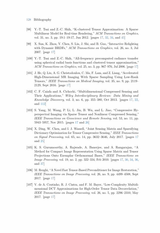
128 Bibliography
[98] Y.-T. Tsai and Z.-C. Shih, “K-clustered Tensor Approximation: A SparseMultilinear Model for Real-time Rendering,” ACM Transactions on Graphics,vol. 31, no. 3, pp. 19:1–19:17, Jun 2012. [pages 17, 32, 34, and 45]
[99] X. Sun, K. Zhou, Y. Chen, S. Lin, J. Shi, and B. Guo, “Interactive Relightingwith Dynamic BRDFs,” ACM Transactions on Graphics, vol. 26, no. 3, Jul2007. [page 17]
[100] Y.-T. Tsai and Z.-C. Shih, “All-frequency precomputed radiance transferusing spherical radial basis functions and clustered tensor approximation,”ACM Transactions on Graphics, vol. 25, no. 3, pp. 967–976, Jul 2006. [page 17]
[101] J. He, Q. Liu, A. G. Christodoulou, C. Ma, F. Lam, and Z. Liang, “AcceleratedHigh-Dimensional MR Imaging With Sparse Sampling Using Low-RankTensors,” IEEE Transactions on Medical Imaging, vol. 35, no. 9, pp. 2119–2129, Sept 2016. [page 17]
[102] C. F. Caiafa and A. Cichocki, “Multidimensional Compressed Sensing andTheir Applications,” Wiley Interdisciplinary Reviews: Data Mining andKnowledge Discovery, vol. 3, no. 6, pp. 355–380, Oct 2013. [pages 17, 22,and 112]
[103] S. Yang, M. Wang, P. Li, L. Jin, B. Wu, and L. Jiao, “Compressive Hy-perspectral Imaging via Sparse Tensor and Nonlinear Compressed Sensing,”IEEE Transactions on Geoscience and Remote Sensing, vol. 53, no. 11, pp.5943–5957, Nov 2015. [pages 17 and 26]
[104] X. Ding, W. Chen, and I. J. Wassell, “Joint Sensing Matrix and SparsifyingDictionary Optimization for Tensor Compressive Sensing,” IEEE Transactionson Signal Processing, vol. 65, no. 14, pp. 3632–3646, July 2017. [pages 17and 25]
[105] K. S. Gurumoorthy, A. Rajwade, A. Banerjee, and A. Rangarajan, “AMethod for Compact Image Representation Using Sparse Matrix and TensorProjections Onto Exemplar Orthonormal Bases,” IEEE Transactions onImage Processing, vol. 19, no. 2, pp. 322–334, Feb 2010. [pages 17, 30, 34, 36,and 37]
[106] M. Rezghi, “A Novel Fast Tensor-Based Preconditioner for Image Restoration,”IEEE Transactions on Image Processing, vol. 26, no. 9, pp. 4499–4508, Sept2017. [page 17]
[107] V. de A. Coutinho, R. J. Cintra, and F. M. Bayer, “Low-Complexity Multidi-mensional DCT Approximations for High-Order Tensor Data Decorrelation,”IEEE Transactions on Image Processing, vol. 26, no. 5, pp. 2296–2310, May2017. [page 17]
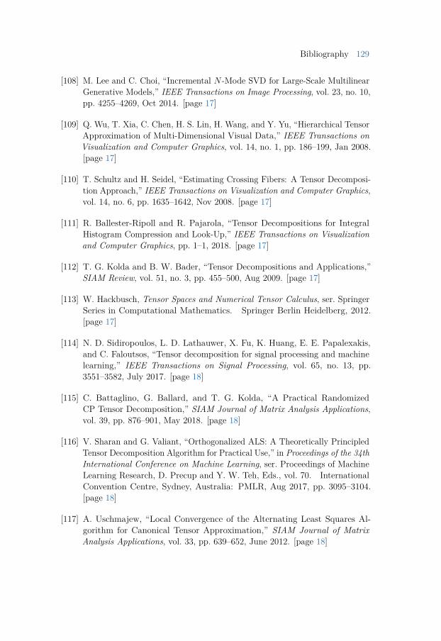
Bibliography 129
[108] M. Lee and C. Choi, “Incremental N -Mode SVD for Large-Scale MultilinearGenerative Models,” IEEE Transactions on Image Processing, vol. 23, no. 10,pp. 4255–4269, Oct 2014. [page 17]
[109] Q. Wu, T. Xia, C. Chen, H. S. Lin, H. Wang, and Y. Yu, “Hierarchical TensorApproximation of Multi-Dimensional Visual Data,” IEEE Transactions onVisualization and Computer Graphics, vol. 14, no. 1, pp. 186–199, Jan 2008.[page 17]
[110] T. Schultz and H. Seidel, “Estimating Crossing Fibers: A Tensor Decomposi-tion Approach,” IEEE Transactions on Visualization and Computer Graphics,vol. 14, no. 6, pp. 1635–1642, Nov 2008. [page 17]
[111] R. Ballester-Ripoll and R. Pajarola, “Tensor Decompositions for IntegralHistogram Compression and Look-Up,” IEEE Transactions on Visualizationand Computer Graphics, pp. 1–1, 2018. [page 17]
[112] T. G. Kolda and B. W. Bader, “Tensor Decompositions and Applications,”SIAM Review, vol. 51, no. 3, pp. 455–500, Aug 2009. [page 17]
[113] W. Hackbusch, Tensor Spaces and Numerical Tensor Calculus, ser. SpringerSeries in Computational Mathematics. Springer Berlin Heidelberg, 2012.[page 17]
[114] N. D. Sidiropoulos, L. D. Lathauwer, X. Fu, K. Huang, E. E. Papalexakis,and C. Faloutsos, “Tensor decomposition for signal processing and machinelearning,” IEEE Transactions on Signal Processing, vol. 65, no. 13, pp.3551–3582, July 2017. [page 18]
[115] C. Battaglino, G. Ballard, and T. G. Kolda, “A Practical RandomizedCP Tensor Decomposition,” SIAM Journal of Matrix Analysis Applications,vol. 39, pp. 876–901, May 2018. [page 18]
[116] V. Sharan and G. Valiant, “Orthogonalized ALS: A Theoretically PrincipledTensor Decomposition Algorithm for Practical Use,” in Proceedings of the 34thInternational Conference on Machine Learning, ser. Proceedings of MachineLearning Research, D. Precup and Y. W. Teh, Eds., vol. 70. InternationalConvention Centre, Sydney, Australia: PMLR, Aug 2017, pp. 3095–3104.[page 18]
[117] A. Uschmajew, “Local Convergence of the Alternating Least Squares Al-gorithm for Canonical Tensor Approximation,” SIAM Journal of MatrixAnalysis Applications, vol. 33, pp. 639–652, June 2012. [page 18]
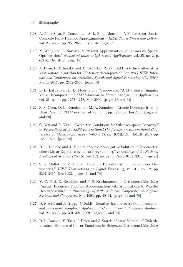
130 Bibliography
[118] A. P. da Silva, P. Comon, and A. L. F. de Almeida, “A Finite Algorithm toCompute Rank-1 Tensor Approximations,” IEEE Signal Processing Letters,vol. 23, no. 7, pp. 959–963, July 2016. [page 18]
[119] X. Wang and C. Navasca, “Low-rank Approximation of Tensors via SparseOptimization,” Numerical Linear Algebra with Applications, vol. 25, no. 2, p.e2136, Dec 2017. [page 18]
[120] A. Phan, P. Tichavský, and A. Cichocki, “Partitioned Hierarchical alternatingleast squares algorithm for CP tensor decomposition,” in 2017 IEEE Inter-national Conference on Acoustics, Speech and Signal Processing (ICASSP),March 2017, pp. 2542–2546. [page 18]
[121] L. D. Lathauwer, B. D. Moor, and J. Vandewalle, “A Multilinear SingularValue Decomposition,” SIAM Journal on Matrix Analysis and Applications,vol. 21, no. 4, pp. 1253–1278, Mar 2000. [pages 18 and 32]
[122] S. S. Chen, D. L. Donoho, and M. A. Saunders, “Atomic Decomposition byBasis Pursuit,” SIAM Review, vol. 43, no. 1, pp. 129–159, Jan 2001. [pages 20and 60]
[123] C. You and R. Vidal, “Geometric Conditions for Subspace-sparse Recovery,”in Proceedings of the 32Nd International Conference on International Con-ference on Machine Learning - Volume 37, ser. ICML’15. JMLR, 2015, pp.1585–1593. [page 20]
[124] D. L. Donoho and J. Tanner, “Sparse Nonnegative Solution of Underdeter-mined Linear Equations by Linear Programming,” Proceedings of the NationalAcademy of Sciences (PNAS), vol. 102, no. 27, pp. 9446–9451, 2005. [page 20]
[125] S. G. Mallat and Z. Zhang, “Matching Pursuits with Time-frequency Dic-tionaries,” IEEE Transactions on Signal Processing, vol. 41, no. 12, pp.3397–3415, Dec 1993. [pages 21 and 70]
[126] Y. C. Pati, R. Rezaiifar, and P. S. Krishnaprasad, “Orthogonal MatchingPursuit: Recursive Function Approximation with Applications to WaveletDecomposition,” in Proceedings of 27th Asilomar Conference on Signals,Systems and Computers, Nov 1993, pp. 40–44. [pages 21 and 70]
[127] D. Needell and J. Tropp, “CoSaMP: Iterative signal recovery from incompleteand inaccurate samples,” Applied and Computational Harmonic Analysis,vol. 26, no. 3, pp. 301–321, 2009. [pages 21 and 70]
[128] D. L. Donoho, Y. Tsaig, I. Drori, and J. Starck, “Sparse Solution of Underde-termined Systems of Linear Equations by Stagewise Orthogonal Matching
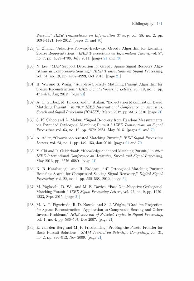
Bibliography 131
Pursuit,” IEEE Transactions on Information Theory, vol. 58, no. 2, pp.1094–1121, Feb 2012. [pages 21 and 70]
[129] T. Zhang, “Adaptive Forward-Backward Greedy Algorithm for LearningSparse Representations,” IEEE Transactions on Information Theory, vol. 57,no. 7, pp. 4689–4708, July 2011. [pages 21 and 70]
[130] N. Lee, “MAP Support Detection for Greedy Sparse Signal Recovery Algo-rithms in Compressive Sensing,” IEEE Transactions on Signal Processing,vol. 64, no. 19, pp. 4987–4999, Oct 2016. [page 21]
[131] H. Wu and S. Wang, “Adaptive Sparsity Matching Pursuit Algorithm forSparse Reconstruction,” IEEE Signal Processing Letters, vol. 19, no. 8, pp.471–474, Aug 2012. [page 21]
[132] A. C. Gurbuz, M. Pilanci, and O. Arikan, “Expectation Maximization BasedMatching Pursuit,” in 2012 IEEE International Conference on Acoustics,Speech and Signal Processing (ICASSP), March 2012, pp. 3313–3316. [page 21]
[133] S. K. Sahoo and A. Makur, “Signal Recovery from Random Measurementsvia Extended Orthogonal Matching Pursuit,” IEEE Transactions on SignalProcessing, vol. 63, no. 10, pp. 2572–2581, May 2015. [pages 21 and 70]
[134] A. Adler, “Covariance-Assisted Matching Pursuit,” IEEE Signal ProcessingLetters, vol. 23, no. 1, pp. 149–153, Jan 2016. [pages 21 and 70]
[135] Y. Chi and R. Calderbank, “Knowledge-enhanced Matching Pursuit,” in 2013IEEE International Conference on Acoustics, Speech and Signal Processing,May 2013, pp. 6576–6580. [page 21]
[136] N. B. Karahanoglu and H. Erdogan, “A∗ Orthogonal Matching Pursuit:Best-first Search for Compressed Sensing Signal Recovery,” Digital SignalProcessing, vol. 22, no. 4, pp. 555–568, 2012. [page 21]
[137] M. Yaghoobi, D. Wu, and M. E. Davies, “Fast Non-Negative OrthogonalMatching Pursuit,” IEEE Signal Processing Letters, vol. 22, no. 9, pp. 1229–1233, Sept 2015. [page 21]
[138] M. A. T. Figueiredo, R. D. Nowak, and S. J. Wright, “Gradient Projectionfor Sparse Reconstruction: Application to Compressed Sensing and OtherInverse Problems,” IEEE Journal of Selected Topics in Signal Processing,vol. 1, no. 4, pp. 586–597, Dec 2007. [page 21]
[139] E. van den Berg and M. P. Friedlander, “Probing the Pareto Frontier forBasis Pursuit Solutions,” SIAM Journal on Scientific Computing, vol. 31,no. 2, pp. 890–912, Nov 2009. [page 21]
132 Bibliography
[140] S. J. Wright, R. D. Nowak, and M. A. T. Figueiredo, “Sparse Reconstructionby Separable Approximation,” IEEE Transactions on Signal Processing,vol. 57, no. 7, pp. 2479–2493, July 2009. [page 21]
[141] B. Efron, T. Hastie, I. Johnstone, and R. Tibshirani, “Least Angle Regression,”Annals of Statistics, vol. 32, no. 2, pp. 407–499, 2004. [page 21]
[142] S. Kim, K. Koh, M. Lustig, S. Boyd, and D. Gorinevsky, “An Interior-PointMethod for Large-Scale `1-Regularized Least Squares,” IEEE Journal ofSelected Topics in Signal Processing, vol. 1, no. 4, pp. 606–617, Dec 2007.[page 21]
[143] Z. Yang, C. Zhang, J. Deng, and W. Lu, “Orthonormal Expansion`1-Minimization Algorithms for Compressed Sensing,” IEEE Transactions onSignal Processing, vol. 59, no. 12, pp. 6285–6290, Dec 2011. [page 21]
[144] M. A. Khajehnejad, W. Xu, A. S. Avestimehr, and B. Hassibi, “Improvingthe Thresholds of Sparse Recovery: An Analysis of a Two-Step ReweightedBasis Pursuit Algorithm,” IEEE Transactions on Information Theory, vol. 61,no. 9, pp. 5116–5128, Sept 2015. [page 21]
[145] J. Yang and Y. Zhang, “Alternating Direction Algorithms for `1-Problems inCompressive Sensing,” SIAM Journal on Scientific Computing, vol. 33, no. 1,pp. 250–278, Feb 2011. [page 21]
[146] H. Liu, B. Song, H. Qin, and Z. Qiu, “An adaptive-admm algorithm withsupport and signal value detection for compressed sensing,” IEEE SignalProcessing Letters, vol. 20, no. 4, pp. 315–318, April 2013. [page 21]
[147] J. F. C. Mota, J. M. F. Xavier, P. M. Q. Aguiar, and M. Puschel, “DistributedBasis Pursuit,” IEEE Transactions on Signal Processing, vol. 60, no. 4, pp.1942–1956, April 2012. [page 21]
[148] Z. Zhang, Y. Xu, J. Yang, X. Li, and D. Zhang, “A survey of sparse repre-sentation: Algorithms and applications,” IEEE Access, vol. 3, pp. 490–530,May 2015. [page 21]
[149] A. Mehranian, H. S. Rad, A. Rahmim, M. R. Ay, and H. Zaidi, “SmoothlyClipped Absolute Deviation (SCAD) Regularization for Compressed SensingMRI Using an Augmented Lagrangian Scheme,” Magnetic Resonance Imaging,vol. 31, no. 8, pp. 1399–1411, 2013. [page 22]
[150] Y.-R. Fan, A. Buccini, M. Donatelli, and T.-Z. Huang, “A Non-convex Regu-larization Approach for Compressive Sensing,” Advances in ComputationalMathematics, Aug 2018. [page 22]
Bibliography 133
[151] C.-H. Zhang, “Nearly Unbiased Variable Selection Under Minimax ConcavePenalty,” The Annals of Statistics, vol. 38, no. 2, pp. 894–942, April 2010.[page 22]
[152] T. Blumensath and M. E. Davies, “Iterative Thresholding for Sparse Approx-imations,” Journal of Fourier Analysis and Applications, vol. 14, no. 5, pp.629–654, Dec 2008. [page 22]
[153] D. Peleg and R. Meir, “A Bilinear Formulation for Vector Sparsity Optimiza-tion,” Signal Processing, vol. 88, no. 2, pp. 375–389, 2008. [page 22]
[154] I. F. Gorodnitsky and B. D. Rao, “Sparse Signal Reconstruction from LimitedData Using FOCUSS: A Re-weighted Minimum Norm Algorithm,” IEEETransactions on Signal Processing, vol. 45, no. 3, pp. 600–616, March 1997.[page 22]
[155] E. J. Candès, M. B. Wakin, and S. P. Boyd, “Enhancing Sparsity byReweighted `1 Minimization,” Journal of Fourier Analysis and Applications,vol. 14, no. 5, pp. 877–905, Dec 2008. [page 22]
[156] C. F. Caiafa and A. Cichocki, “Computing Sparse Representations of Multi-dimensional Signals Using Kronecker Bases,” Neural Compututation, vol. 25,no. 1, pp. 186–220, Jan 2013. [page 22]
[157] Y. C. Eldar, P. Kuppinger, and H. Bolcskei, “Block-Sparse Signals: Un-certainty Relations and Efficient Recovery,” IEEE Transactions on SignalProcessing, vol. 58, no. 6, pp. 3042–3054, June 2010. [pages 22 and 66]
[158] X. Ding, W. Chen, and I. Wassell, “Nonconvex Compressive Sensing Recon-struction for Tensor Using Structures in Modes,” in 2016 IEEE InternationalConference on Acoustics, Speech and Signal Processing (ICASSP), March2016, pp. 4658–4662. [page 22]
[159] N. D. Sidiropoulos and A. Kyrillidis, “Multi-Way Compressed Sensing forSparse Low-Rank Tensors,” IEEE Signal Processing Letters, vol. 19, no. 11,pp. 757–760, Nov 2012. [page 22]
[160] S. Friedland, Q. Li, and D. Schonfeld, “Compressive Sensing of SparseTensors,” IEEE Transactions on Image Processing, vol. 23, no. 10, pp. 4438–4447, Oct 2014. [pages 22 and 104]
[161] W. Dai, Y. Li, J. Zou, H. Xiong, and Y. F. Zheng, “Fully DecomposableCompressive Sampling With Joint Optimization for Multidimensional SparseRepresentation,” IEEE Transactions on Signal Processing, vol. 66, no. 3, pp.603–616, Feb 2018. [page 22]
134 Bibliography
[162] M. Aharon, M. Elad, and A. Bruckstein, “K-SVD: An Algorithm for DesigningOvercomplete Dictionaries for Sparse Representation,” IEEE Transactionson Signal Processing, vol. 54, no. 11, pp. 4311–4322, Nov 2006. [pages 22, 34,and 43]
[163] R. Rubinstein, M. Zibulevsky, and M. Elad, “Efficient Implementation of theK-SVD Algorithm Using Batch Orthogonal Matching Pursuit,” ComputerScience Department, Technion–Israel Institute of Technology, Tech. Rep.,Aug 2008. [page 23]
[164] J. Mairal, F. Bach, J. Ponce, and G. Sapiro, “Online Dictionary Learning forSparse Coding,” in Proceedings of the 26th Annual International Conferenceon Machine Learning, ser. ICML ’09, 2009, pp. 689–696. [pages 24, 95,and 108]
[165] S. Mukherjee, R. Basu, and C. S. Seelamantula, “`1-K-SVD: A robust dictio-nary learning algorithm with simultaneous update,” Signal Processing, vol.123, pp. 42–52, June 2016. [pages 24 and 43]
[166] M. Yaghoobi, T. Blumensath, and M. E. Davies, “Dictionary Learning forSparse Approximations With the Majorization Method,” IEEE Transactionson Signal Processing, vol. 57, no. 6, pp. 2178–2191, June 2009. [page 24]
[167] D. Barchiesi and M. D. Plumbley, “Learning Incoherent Dictionaries forSparse Approximation Using Iterative Projections and Rotations,” IEEETransactions on Signal Processing, vol. 61, no. 8, pp. 2055–2065, April 2013.[page 24]
[168] B. Wen, S. Ravishankar, and Y. Bresler, “Learning Flipping and RotationInvariant Sparsifying Transforms,” in 2016 IEEE International Conferenceon Image Processing (ICIP), Sept 2016, pp. 3857–3861. [page 24]
[169] A. Abdi, A. Payani, and F. Fekri, “Learning Dictionary for Efficient SignalCompression,” in 2017 IEEE International Conference on Acoustics, Speechand Signal Processing (ICASSP), March 2017, pp. 3689–3693. [page 24]
[170] C. Studer and R. G. Baraniuk, “Dictionary Learning From Sparsely Corruptedor Compressed Signals,” in 2012 IEEE International Conference on Acoustics,Speech and Signal Processing (ICASSP), March 2012, pp. 3341–3344. [page 24]
[171] Z. Sadeghipoor, M. Babaie-Zadeh, and C. Jutten, “Dictionary Learning forSparse Decomposition: A New Criterion and Algorithm,” in 2013 IEEEInternational Conference on Acoustics, Speech and Signal Processing, May2013, pp. 5855–5859. [page 24]
Bibliography 135
[172] R. Mazhar and P. D. Gader, “EK-SVD: Optimized Dictionary Design forSparse Representations,” in 2008 19th International Conference on PatternRecognition, Dec 2008, pp. 1–4. [pages 24 and 43]
[173] J. Feng, L. Song, X. Yang, and W. Zhang, “Sub Clustering K-SVD: SizeVariable Dictionary Learning for Sparse Representations,” in 2009 16thIEEE International Conference on Image Processing (ICIP), Nov 2009, pp.2149–2152. [page 24]
[174] C. Rusu and B. Dumitrescu, “Stagewise K-SVD to Design Efficient Dictio-naries for Sparse Representations,” IEEE Signal Processing Letters, vol. 19,no. 10, pp. 631–634, Oct 2012. [page 24]
[175] M. Marsousi, K. Abhari, P. Babyn, and J. Alirezaie, “An Adaptive Approachto Learn Overcomplete Dictionaries With Efficient Numbers of Elements,”IEEE Transactions on Signal Processing, vol. 62, no. 12, pp. 3272–3283, June2014. [pages 24 and 43]
[176] Z. Jiang, Z. Lin, and L. S. Davis, “Label Consistent K-SVD: Learning aDiscriminative Dictionary for Recognition,” IEEE Transactions on PatternAnalysis and Machine Intelligence, vol. 35, no. 11, pp. 2651–2664, Nov 2013.[page 24]
[177] J. Mairal, F. Bach, and J. Ponce, “Task-Driven Dictionary Learning,” IEEETransactions on Pattern Analysis and Machine Intelligence, vol. 34, no. 4,pp. 791–804, April 2012. [page 24]
[178] Z. You, R. Raich, X. Z. Fern, and J. Kim, “Weakly Supervised DictionaryLearning,” IEEE Transactions on Signal Processing, vol. 66, no. 10, pp.2527–2541, May 2018. [page 24]
[179] Y. Sun, Q. Liu, J. Tang, and D. Tao, “Learning Discriminative Dictionaryfor Group Sparse Representation,” IEEE Transactions on Image Processing,vol. 23, no. 9, pp. 3816–3828, Sept 2014. [page 24]
[180] M. J. Gangeh, A. Ghodsi, and M. S. Kamel, “Kernelized Supervised Dictio-nary Learning,” IEEE Transactions on Signal Processing, vol. 61, no. 19, pp.4753–4767, Oct 2013. [page 24]
[181] N. Zhou, Y. Shen, J. Peng, and J. Fan, “Learning Inter-related VisualDictionary for Object Recognition,” in 2012 IEEE Conference on ComputerVision and Pattern Recognition (CVPR), June 2012, pp. 3490–3497. [page 24]
[182] Z. Zhang, F. Li, T. W. S. Chow, L. Zhang, and S. Yan, “Sparse Codes Auto-Extractor for Classification: A Joint Embedding and Dictionary Learning
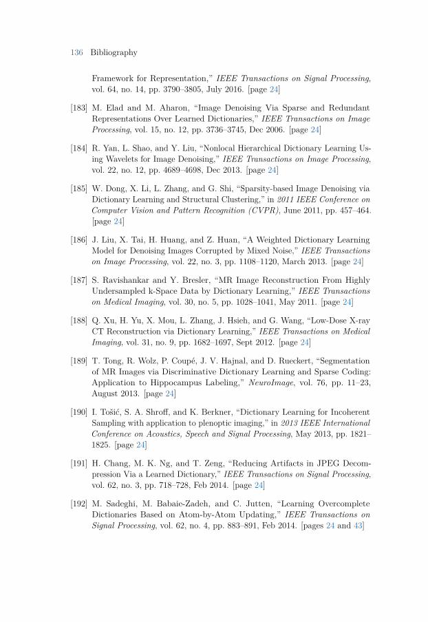
136 Bibliography
Framework for Representation,” IEEE Transactions on Signal Processing,vol. 64, no. 14, pp. 3790–3805, July 2016. [page 24]
[183] M. Elad and M. Aharon, “Image Denoising Via Sparse and RedundantRepresentations Over Learned Dictionaries,” IEEE Transactions on ImageProcessing, vol. 15, no. 12, pp. 3736–3745, Dec 2006. [page 24]
[184] R. Yan, L. Shao, and Y. Liu, “Nonlocal Hierarchical Dictionary Learning Us-ing Wavelets for Image Denoising,” IEEE Transactions on Image Processing,vol. 22, no. 12, pp. 4689–4698, Dec 2013. [page 24]
[185] W. Dong, X. Li, L. Zhang, and G. Shi, “Sparsity-based Image Denoising viaDictionary Learning and Structural Clustering,” in 2011 IEEE Conference onComputer Vision and Pattern Recognition (CVPR), June 2011, pp. 457–464.[page 24]
[186] J. Liu, X. Tai, H. Huang, and Z. Huan, “A Weighted Dictionary LearningModel for Denoising Images Corrupted by Mixed Noise,” IEEE Transactionson Image Processing, vol. 22, no. 3, pp. 1108–1120, March 2013. [page 24]
[187] S. Ravishankar and Y. Bresler, “MR Image Reconstruction From HighlyUndersampled k-Space Data by Dictionary Learning,” IEEE Transactionson Medical Imaging, vol. 30, no. 5, pp. 1028–1041, May 2011. [page 24]
[188] Q. Xu, H. Yu, X. Mou, L. Zhang, J. Hsieh, and G. Wang, “Low-Dose X-rayCT Reconstruction via Dictionary Learning,” IEEE Transactions on MedicalImaging, vol. 31, no. 9, pp. 1682–1697, Sept 2012. [page 24]
[189] T. Tong, R. Wolz, P. Coupé, J. V. Hajnal, and D. Rueckert, “Segmentationof MR Images via Discriminative Dictionary Learning and Sparse Coding:Application to Hippocampus Labeling,” NeuroImage, vol. 76, pp. 11–23,August 2013. [page 24]
[190] I. Tošić, S. A. Shroff, and K. Berkner, “Dictionary Learning for IncoherentSampling with application to plenoptic imaging,” in 2013 IEEE InternationalConference on Acoustics, Speech and Signal Processing, May 2013, pp. 1821–1825. [page 24]
[191] H. Chang, M. K. Ng, and T. Zeng, “Reducing Artifacts in JPEG Decom-pression Via a Learned Dictionary,” IEEE Transactions on Signal Processing,vol. 62, no. 3, pp. 718–728, Feb 2014. [page 24]
[192] M. Sadeghi, M. Babaie-Zadeh, and C. Jutten, “Learning OvercompleteDictionaries Based on Atom-by-Atom Updating,” IEEE Transactions onSignal Processing, vol. 62, no. 4, pp. 883–891, Feb 2014. [pages 24 and 43]
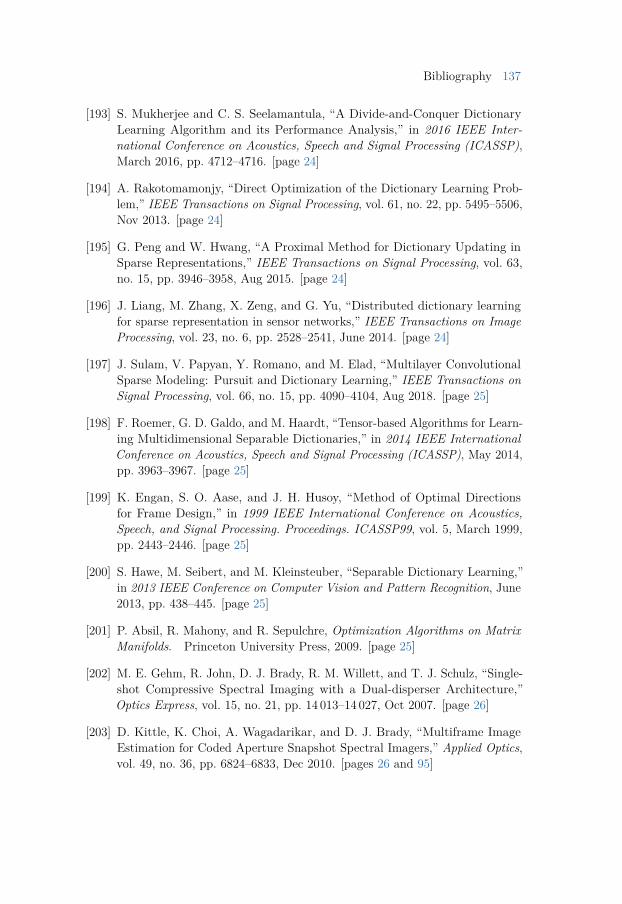
Bibliography 137
[193] S. Mukherjee and C. S. Seelamantula, “A Divide-and-Conquer DictionaryLearning Algorithm and its Performance Analysis,” in 2016 IEEE Inter-national Conference on Acoustics, Speech and Signal Processing (ICASSP),March 2016, pp. 4712–4716. [page 24]
[194] A. Rakotomamonjy, “Direct Optimization of the Dictionary Learning Prob-lem,” IEEE Transactions on Signal Processing, vol. 61, no. 22, pp. 5495–5506,Nov 2013. [page 24]
[195] G. Peng and W. Hwang, “A Proximal Method for Dictionary Updating inSparse Representations,” IEEE Transactions on Signal Processing, vol. 63,no. 15, pp. 3946–3958, Aug 2015. [page 24]
[196] J. Liang, M. Zhang, X. Zeng, and G. Yu, “Distributed dictionary learningfor sparse representation in sensor networks,” IEEE Transactions on ImageProcessing, vol. 23, no. 6, pp. 2528–2541, June 2014. [page 24]
[197] J. Sulam, V. Papyan, Y. Romano, and M. Elad, “Multilayer ConvolutionalSparse Modeling: Pursuit and Dictionary Learning,” IEEE Transactions onSignal Processing, vol. 66, no. 15, pp. 4090–4104, Aug 2018. [page 25]
[198] F. Roemer, G. D. Galdo, and M. Haardt, “Tensor-based Algorithms for Learn-ing Multidimensional Separable Dictionaries,” in 2014 IEEE InternationalConference on Acoustics, Speech and Signal Processing (ICASSP), May 2014,pp. 3963–3967. [page 25]
[199] K. Engan, S. O. Aase, and J. H. Husoy, “Method of Optimal Directionsfor Frame Design,” in 1999 IEEE International Conference on Acoustics,Speech, and Signal Processing. Proceedings. ICASSP99, vol. 5, March 1999,pp. 2443–2446. [page 25]
[200] S. Hawe, M. Seibert, and M. Kleinsteuber, “Separable Dictionary Learning,”in 2013 IEEE Conference on Computer Vision and Pattern Recognition, June2013, pp. 438–445. [page 25]
[201] P. Absil, R. Mahony, and R. Sepulchre, Optimization Algorithms on MatrixManifolds. Princeton University Press, 2009. [page 25]
[202] M. E. Gehm, R. John, D. J. Brady, R. M. Willett, and T. J. Schulz, “Single-shot Compressive Spectral Imaging with a Dual-disperser Architecture,”Optics Express, vol. 15, no. 21, pp. 14 013–14 027, Oct 2007. [page 26]
[203] D. Kittle, K. Choi, A. Wagadarikar, and D. J. Brady, “Multiframe ImageEstimation for Coded Aperture Snapshot Spectral Imagers,” Applied Optics,vol. 49, no. 36, pp. 6824–6833, Dec 2010. [pages 26 and 95]
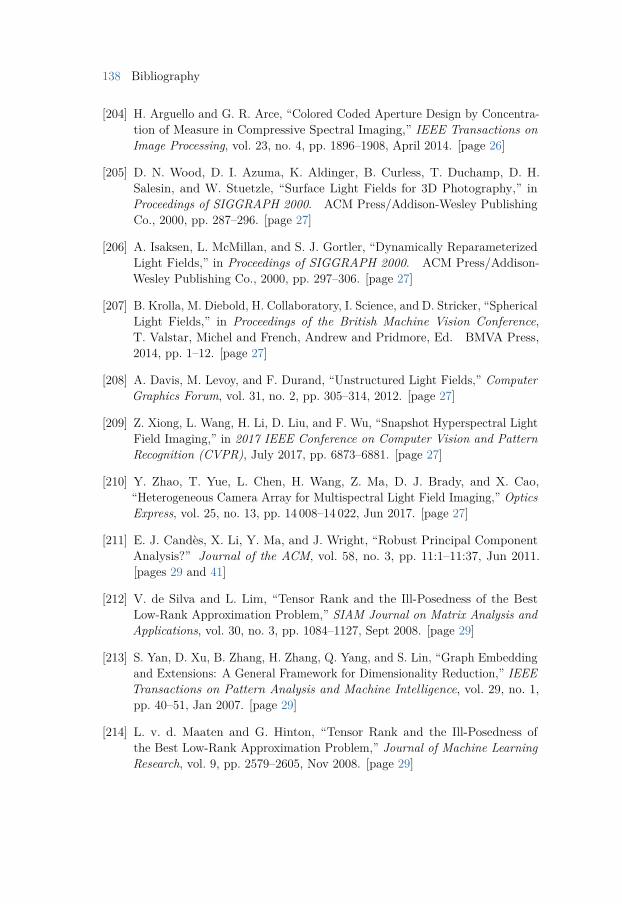
138 Bibliography
[204] H. Arguello and G. R. Arce, “Colored Coded Aperture Design by Concentra-tion of Measure in Compressive Spectral Imaging,” IEEE Transactions onImage Processing, vol. 23, no. 4, pp. 1896–1908, April 2014. [page 26]
[205] D. N. Wood, D. I. Azuma, K. Aldinger, B. Curless, T. Duchamp, D. H.Salesin, and W. Stuetzle, “Surface Light Fields for 3D Photography,” inProceedings of SIGGRAPH 2000. ACM Press/Addison-Wesley PublishingCo., 2000, pp. 287–296. [page 27]
[206] A. Isaksen, L. McMillan, and S. J. Gortler, “Dynamically ReparameterizedLight Fields,” in Proceedings of SIGGRAPH 2000. ACM Press/Addison-Wesley Publishing Co., 2000, pp. 297–306. [page 27]
[207] B. Krolla, M. Diebold, H. Collaboratory, I. Science, and D. Stricker, “SphericalLight Fields,” in Proceedings of the British Machine Vision Conference,T. Valstar, Michel and French, Andrew and Pridmore, Ed. BMVA Press,2014, pp. 1–12. [page 27]
[208] A. Davis, M. Levoy, and F. Durand, “Unstructured Light Fields,” ComputerGraphics Forum, vol. 31, no. 2, pp. 305–314, 2012. [page 27]
[209] Z. Xiong, L. Wang, H. Li, D. Liu, and F. Wu, “Snapshot Hyperspectral LightField Imaging,” in 2017 IEEE Conference on Computer Vision and PatternRecognition (CVPR), July 2017, pp. 6873–6881. [page 27]
[210] Y. Zhao, T. Yue, L. Chen, H. Wang, Z. Ma, D. J. Brady, and X. Cao,“Heterogeneous Camera Array for Multispectral Light Field Imaging,” OpticsExpress, vol. 25, no. 13, pp. 14 008–14 022, Jun 2017. [page 27]
[211] E. J. Candès, X. Li, Y. Ma, and J. Wright, “Robust Principal ComponentAnalysis?” Journal of the ACM, vol. 58, no. 3, pp. 11:1–11:37, Jun 2011.[pages 29 and 41]
[212] V. de Silva and L. Lim, “Tensor Rank and the Ill-Posedness of the BestLow-Rank Approximation Problem,” SIAM Journal on Matrix Analysis andApplications, vol. 30, no. 3, pp. 1084–1127, Sept 2008. [page 29]
[213] S. Yan, D. Xu, B. Zhang, H. Zhang, Q. Yang, and S. Lin, “Graph Embeddingand Extensions: A General Framework for Dimensionality Reduction,” IEEETransactions on Pattern Analysis and Machine Intelligence, vol. 29, no. 1,pp. 40–51, Jan 2007. [page 29]
[214] L. v. d. Maaten and G. Hinton, “Tensor Rank and the Ill-Posedness ofthe Best Low-Rank Approximation Problem,” Journal of Machine LearningResearch, vol. 9, pp. 2579–2605, Nov 2008. [page 29]
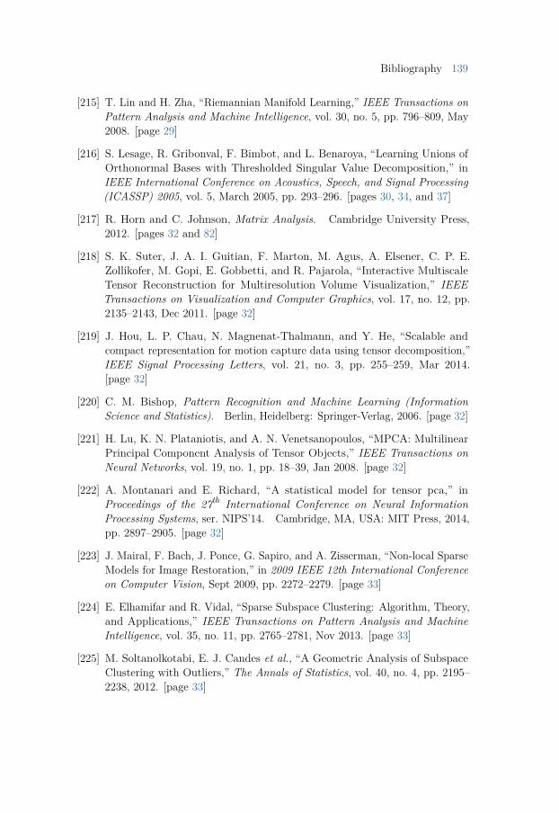
Bibliography 139
[215] T. Lin and H. Zha, “Riemannian Manifold Learning,” IEEE Transactions onPattern Analysis and Machine Intelligence, vol. 30, no. 5, pp. 796–809, May2008. [page 29]
[216] S. Lesage, R. Gribonval, F. Bimbot, and L. Benaroya, “Learning Unions ofOrthonormal Bases with Thresholded Singular Value Decomposition,” inIEEE International Conference on Acoustics, Speech, and Signal Processing(ICASSP) 2005, vol. 5, March 2005, pp. 293–296. [pages 30, 34, and 37]
[217] R. Horn and C. Johnson, Matrix Analysis. Cambridge University Press,2012. [pages 32 and 82]
[218] S. K. Suter, J. A. I. Guitian, F. Marton, M. Agus, A. Elsener, C. P. E.Zollikofer, M. Gopi, E. Gobbetti, and R. Pajarola, “Interactive MultiscaleTensor Reconstruction for Multiresolution Volume Visualization,” IEEETransactions on Visualization and Computer Graphics, vol. 17, no. 12, pp.2135–2143, Dec 2011. [page 32]
[219] J. Hou, L. P. Chau, N. Magnenat-Thalmann, and Y. He, “Scalable andcompact representation for motion capture data using tensor decomposition,”IEEE Signal Processing Letters, vol. 21, no. 3, pp. 255–259, Mar 2014.[page 32]
[220] C. M. Bishop, Pattern Recognition and Machine Learning (InformationScience and Statistics). Berlin, Heidelberg: Springer-Verlag, 2006. [page 32]
[221] H. Lu, K. N. Plataniotis, and A. N. Venetsanopoulos, “MPCA: MultilinearPrincipal Component Analysis of Tensor Objects,” IEEE Transactions onNeural Networks, vol. 19, no. 1, pp. 18–39, Jan 2008. [page 32]
[222] A. Montanari and E. Richard, “A statistical model for tensor pca,” inProceedings of the 27th International Conference on Neural InformationProcessing Systems, ser. NIPS’14. Cambridge, MA, USA: MIT Press, 2014,pp. 2897–2905. [page 32]
[223] J. Mairal, F. Bach, J. Ponce, G. Sapiro, and A. Zisserman, “Non-local SparseModels for Image Restoration,” in 2009 IEEE 12th International Conferenceon Computer Vision, Sept 2009, pp. 2272–2279. [page 33]
[224] E. Elhamifar and R. Vidal, “Sparse Subspace Clustering: Algorithm, Theory,and Applications,” IEEE Transactions on Pattern Analysis and MachineIntelligence, vol. 35, no. 11, pp. 2765–2781, Nov 2013. [page 33]
[225] M. Soltanolkotabi, E. J. Candes et al., “A Geometric Analysis of SubspaceClustering with Outliers,” The Annals of Statistics, vol. 40, no. 4, pp. 2195–2238, 2012. [page 33]
140 Bibliography
[226] D. Mahajan, I. K. Shlizerman, R. Ramamoorthi, and P. Belhumeur, “ATheory of Locally Low Dimensional Light Transport,” ACM Transactions onGraphics, vol. 26, no. 3, Jul 2007. [page 33]
[227] W. Dong, L. Zhang, G. Shi, and X. Li, “Nonlocally Centralized Sparse Rep-resentation for Image Restoration,” IEEE Transactions on Image Processing,vol. 22, no. 4, pp. 1620–1630, April 2013. [page 33]
[228] P.-P. Sloan, J. Hall, J. Hart, and J. Snyder, “Clustered Principal Componentsfor Precomputed Radiance Transfer,” ACM Transactions on Graphics, vol. 22,no. 3, pp. 382–391, Jul 2003. [pages 33, 39, and 45]
[229] K. Schröder, R. Klein, and A. Zinke, “Non-Local Image Reconstructionfor Efficient Computation of Synthetic Bidirectional Texture Functions,”Computer Graphics Forum, vol. 32, no. 8, pp. 61–71, June 2013. [page 33]
[230] M. Guthe, G. Müller, M. Schneider, and R. Klein, “BTF-CIELab: A Percep-tual Difference Measure for Quality Assessment and Compression of BTFs,”Computer Graphics Forum, vol. 28, no. 1, pp. 101–113, 2009. [page 34]
[231] A. Rangarajan, A. Yuille, and E. Mjolsness, “Convergence Properties of theSoftassign Quadratic Assignment Algorithm,” Neural Computation, vol. 11,no. 6, pp. 1455–1474, Aug 1999. [page 36]
[232] J. Kosowsky and A. Yuille, “The Invisible Hand Algorithm: Solving theAssignment Problem with Statistical Physics,” Neural Networks, vol. 7, no. 3,pp. 477–490, 1994. [page 36]
[233] K. B. Petersen and M. S. Pedersen, “The matrix cookbook,” Nov 2012,version 20121115. [page 37]
[234] R. Wang, R. Wang, K. Zhou, M. Pan, and H. Bao, “An Efficient GPU-basedApproach for Interactive Global Illumination,” ACM Transactions Graphics,vol. 28, no. 3, pp. 91:1–91:8, Jul 2009. [page 39]
[235] A. Bock, E. Sundén, B. Liu, B. Wünsche, and T. Ropinski, “Coherency-BasedCurve Compression for High-Order Finite Element Model Visualization,”IEEE Transactions on Visualization and Computer Graphics, vol. 18, no. 12,pp. 2315–2324, Dec 2012. [page 39]
[236] Z. Zheng, N. Ahmed, and K. Mueller, “iView: A Feature Clustering Frame-work for Suggesting Informative Views in Volume Visualization,” IEEETransactions on Visualization and Computer Graphics, vol. 17, no. 12, pp.1959–1968, Dec 2011. [page 39]
Bibliography 141
[237] C. W. Chen, J. Luo, and K. J. Parker, “Image Segmentation via AdaptiveK-mean Clustering and Knowledge-based Morphological Operations withBiomedical Applications,” IEEE Transactions on Image Processing, vol. 7,no. 12, pp. 1673–1683, Dec 1998. [page 39]
[238] A. Y. Ng, M. I. Jordan, and Y. Weiss, “On Spectral Clustering: Analysisand an Algorithm,” in Proceedings of the 14th International Conference onNeural Information Processing Systems, ser. NIPS’01. MIT Press, Dec 2001,pp. 849–856. [page 39]
[239] E. Elhamifar and R. Vidal, “Sparse Subspace Clustering,” in 2009 IEEEConference on Computer Vision and Pattern Recognition, June 2009, pp.2790–2797. [page 39]
[240] H. Xu, C. Caramanis, and S. Mannor, “Outlier-Robust PCA: The High-Dimensional Case,” IEEE Transactions on Information Theory, vol. 59, no. 1,pp. 546–572, Jan 2013. [page 41]
[241] M. Rahmani and G. K. Atia, “Coherence Pursuit: Fast, Simple, and RobustPrincipal Component Analysis,” IEEE Transactions on Signal Processing,vol. 65, no. 23, pp. 6260–6275, Dec 2017. [page 41]
[242] J. Wright, A. Ganesh, S. Rao, Y. Peng, and Y. Ma, “Robust PrincipalComponent Analysis: Exact Recovery of Corrupted Low-Rank Matricesvia Convex Optimization,” in Advances in Neural Information ProcessingSystems (NIPS 2009), Y. Bengio, D. Schuurmans, J. D. Lafferty, C. K. I.Williams, and A. Culotta, Eds. Curran Associates, Inc., 2009, pp. 2080–2088.[page 41]
[243] Y. Fang, L. Chen, J. Wu, and B. Huang, “GPU Implementation of OrthogonalMatching Pursuit for Compressive Sensing,” in 2011 IEEE 17th InternationalConference on Parallel and Distributed Systems, Dec 2011, pp. 1044–1047.[pages 43 and 72]
[244] F. Huang, J. Tao, Y. Xiang, P. Liu, L. Dong, and L. Wang, “ParallelCompressive Sampling Matching Pursuit Algorithm for Compressed SensingSignal Reconstruction with OpenCL,” Journal of Systems Architecture, vol. 72,no. C, pp. 51–60, Jan 2017. [page 43]
[245] J. D. Blanchard and J. Tanner, “GPU Accelerated Greedy Algorithms forCompressed Sensing,” Mathematical Programming Computation, vol. 5, no. 3,pp. 267–304, Sept 2013. [page 43]
[246] C.-L. Chang, X. Zhu, P. Ramanathan, and B. Girod, “Light field com-pression using disparity-compensated lifting and shape adaptation,” IEEE
142 Bibliography
Transactions on Image Processing, vol. 15, no. 4, pp. 793–806, April 2006.[page 45]
[247] N. Fout and K. Ma, “An Adaptive Prediction-Based Approach to LosslessCompression of Floating-Point Volume Data,” IEEE Transactions on Visu-alization and Computer Graphics, vol. 18, no. 12, pp. 2295–2304, Dec 2012.[page 45]
[248] G. Müller, J. Meseth, and R. Klein, “Compression and Real-Time Renderingof Measured BTFs Using Local PCA,” in The 8th International Fall WorkshopVision, Modeling and Visualisation 2003, T. Ertl, B. Girod, G. Greiner, H. Nie-mann, H.-P. Seidel, E. Steinbach, and R. Westermann, Eds. AkademischeVerlagsgesellschaft Aka GmbH, Berlin, Nov 2003, pp. 271–280. [page 45]
[249] A. Appel, “Some Techniques for Shading Machine Renderings of Solids,” inProceedings of the April 30–May 2, 1968, Spring Joint Computer Conference.ACM, 1968, pp. 37–45. [pages 46 and 98]
[250] J. T. Kajiya, “The Rendering Equation,” in Proceedings of SIGGRAPH 1986.ACM, 1986, pp. 143–150. [pages 46 and 98]
[251] S. Lee, E. Eisemann, and H.-P. Seidel, “Real-time Lens Blur Effects andFocus Control,” ACM Transactions Graphics, vol. 29, no. 4, pp. 65:1–65:7,Jul 2010. [page 47]
[252] M. Hullin, E. Eisemann, H.-P. Seidel, and S. Lee, “Physically-based Real-time Lens Flare Rendering,” ACM Transactions Graphics, vol. 30, no. 4, pp.108:1–108:10, Jul 2011. [page 47]
[253] L. Belcour, “Efficient Rendering of Layered Materials Using an AtomicDecomposition with Statistical Operators,” ACM Transactions Graphics,vol. 37, no. 4, pp. 73:1–73:15, Jul 2018. [page 47]
[254] A. Toisoul and A. Ghosh, “Practical Acquisition and Rendering of DiffractionEffects in Surface Reflectance,” ACM Transactions Graphics, vol. 36, no. 4,Jul 2017. [page 47]
[255] I. Sadeghi, A. Munoz, P. Laven, W. Jarosz, F. Seron, D. Gutierrez, andH. W. Jensen, “Physically-based Simulation of Rainbows,” ACM TransactionsGraphics, vol. 31, no. 1, pp. 3:1–3:12, Feb 2012. [page 47]
[256] K. Xu, L.-Q. Ma, B. Ren, R. Wang, and S.-M. Hu, “Interactive Hair Renderingand Appearance Editing Under Environment Lighting,” ACM TransactionsGraphics, vol. 30, no. 6, pp. 173:1–173:10, Dec 2011. [page 47]
Bibliography 143
[257] J. M. Singh and P. J. Narayanan, “Real-Time Ray Tracing of Implicit Surfaceson the GPU,” IEEE Transactions on Visualization and Computer Graphics,vol. 16, no. 2, pp. 261–272, March 2010. [page 47]
[258] I. Wald, H. Friedrich, G. Marmitt, P. Slusallek, and H. P. Seidel, “Fasterisosurface ray tracing using implicit KD-trees,” IEEE Transactions on Vi-sualization and Computer Graphics, vol. 11, no. 5, pp. 562–572, Sept 2005.[page 47]
[259] A. Silvennoinen and J. Lehtinen, “Real-time Global Illumination by Precom-puted Local Reconstruction from Sparse Radiance Probes,” ACM Transac-tions Graphics, vol. 36, no. 6, pp. 230:1–230:13, Nov. 2017. [page 47]
[260] P. Ren, J. Wang, M. Gong, S. Lin, X. Tong, and B. Guo, “Global Illuminationwith Radiance Regression Functions,” ACM Transactions Graphics, vol. 32,no. 4, pp. 130:1–130:12, Jul 2013. [page 47]
[261] P. Shirley and K. Chiu, “A Low Distortion Map Between Disk and Square,”Journal of Graphics Tools, vol. 2, no. 3, pp. 45–52, 1997. [page 48]
[262] N. Sabater, G. Boisson, B. Vandame, P. Kerbiriou, F. Babon, M. Hog,R. Gendrot, T. Langlois, O. Bureller, A. Schubert, and V. Allié, “Datasetand Pipeline for Multi-view Light-Field Video,” in 2017 IEEE Conference onComputer Vision and Pattern Recognition Workshops (CVPRW), July 2017,pp. 1743–1753. [pages 53, 54, 103, and 104]
[263] M. H. Kamal, B. Heshmat, R. Raskar, P. Vandergheynst, and G. Wetzstein,“Tensor low-rank and sparse light field photography,” Computer Vision andImage Understanding, vol. 145, pp. 172–181, 2016, light Field for ComputerVision. [page 52]
[264] J.-D. Durou, M. Falcone, and M. Sagona, “Numerical Methods for Shape-from-shading: A New Survey with Benchmarks,” Computer Vision and ImageUnderstanding, vol. 109, no. 1, pp. 22–43, Jan 2008. [page 55]
[265] Lucas Digital Ltd. LLC., Technical Introduction to OpenEXR, Nov 2006.[page 55]
[266] I. Ihm, S. Park, and R. K. Lee, “Rendering of Spherical Light Fields,”in Proceedings The Fifth Pacific Conference on Computer Graphics andApplications, Oct 1997, pp. 59–68. [page 57]
[267] F. Marvasti, Ed., Nonuniform Sampling: Theory and Practice, ser. Informa-tion Technology: Transmission, Processing and Storage. Springer US, 2001.[page 59]
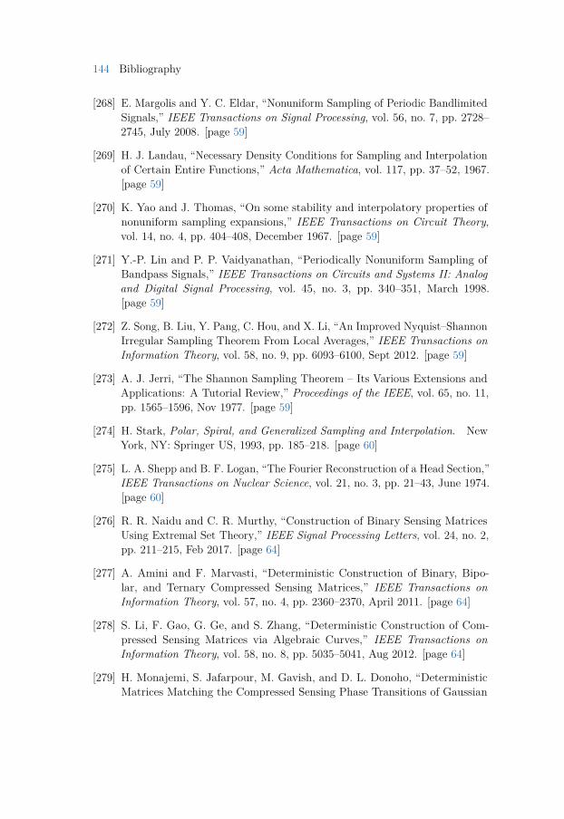
144 Bibliography
[268] E. Margolis and Y. C. Eldar, “Nonuniform Sampling of Periodic BandlimitedSignals,” IEEE Transactions on Signal Processing, vol. 56, no. 7, pp. 2728–2745, July 2008. [page 59]
[269] H. J. Landau, “Necessary Density Conditions for Sampling and Interpolationof Certain Entire Functions,” Acta Mathematica, vol. 117, pp. 37–52, 1967.[page 59]
[270] K. Yao and J. Thomas, “On some stability and interpolatory properties ofnonuniform sampling expansions,” IEEE Transactions on Circuit Theory,vol. 14, no. 4, pp. 404–408, December 1967. [page 59]
[271] Y.-P. Lin and P. P. Vaidyanathan, “Periodically Nonuniform Sampling ofBandpass Signals,” IEEE Transactions on Circuits and Systems II: Analogand Digital Signal Processing, vol. 45, no. 3, pp. 340–351, March 1998.[page 59]
[272] Z. Song, B. Liu, Y. Pang, C. Hou, and X. Li, “An Improved Nyquist–ShannonIrregular Sampling Theorem From Local Averages,” IEEE Transactions onInformation Theory, vol. 58, no. 9, pp. 6093–6100, Sept 2012. [page 59]
[273] A. J. Jerri, “The Shannon Sampling Theorem – Its Various Extensions andApplications: A Tutorial Review,” Proceedings of the IEEE, vol. 65, no. 11,pp. 1565–1596, Nov 1977. [page 59]
[274] H. Stark, Polar, Spiral, and Generalized Sampling and Interpolation. NewYork, NY: Springer US, 1993, pp. 185–218. [page 60]
[275] L. A. Shepp and B. F. Logan, “The Fourier Reconstruction of a Head Section,”IEEE Transactions on Nuclear Science, vol. 21, no. 3, pp. 21–43, June 1974.[page 60]
[276] R. R. Naidu and C. R. Murthy, “Construction of Binary Sensing MatricesUsing Extremal Set Theory,” IEEE Signal Processing Letters, vol. 24, no. 2,pp. 211–215, Feb 2017. [page 64]
[277] A. Amini and F. Marvasti, “Deterministic Construction of Binary, Bipo-lar, and Ternary Compressed Sensing Matrices,” IEEE Transactions onInformation Theory, vol. 57, no. 4, pp. 2360–2370, April 2011. [page 64]
[278] S. Li, F. Gao, G. Ge, and S. Zhang, “Deterministic Construction of Com-pressed Sensing Matrices via Algebraic Curves,” IEEE Transactions onInformation Theory, vol. 58, no. 8, pp. 5035–5041, Aug 2012. [page 64]
[279] H. Monajemi, S. Jafarpour, M. Gavish, and D. L. Donoho, “DeterministicMatrices Matching the Compressed Sensing Phase Transitions of Gaussian
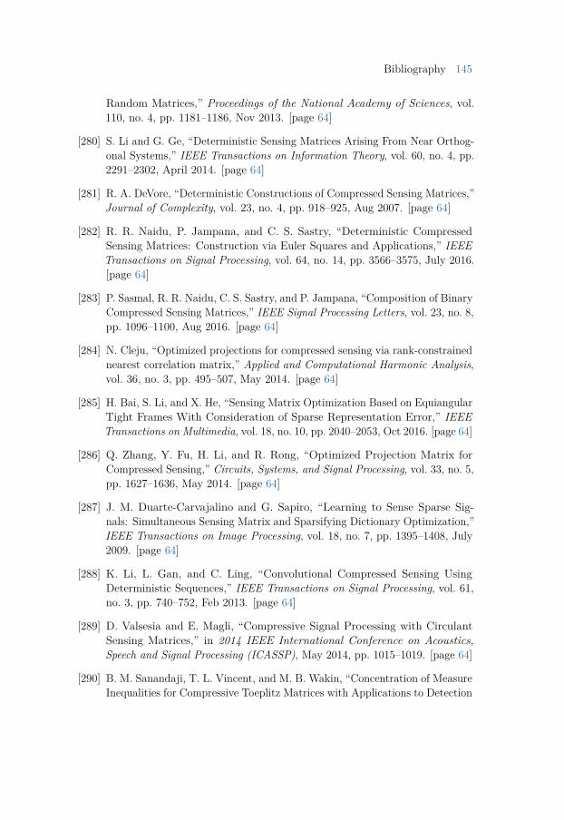
Bibliography 145
Random Matrices,” Proceedings of the National Academy of Sciences, vol.110, no. 4, pp. 1181–1186, Nov 2013. [page 64]
[280] S. Li and G. Ge, “Deterministic Sensing Matrices Arising From Near Orthog-onal Systems,” IEEE Transactions on Information Theory, vol. 60, no. 4, pp.2291–2302, April 2014. [page 64]
[281] R. A. DeVore, “Deterministic Constructions of Compressed Sensing Matrices,”Journal of Complexity, vol. 23, no. 4, pp. 918–925, Aug 2007. [page 64]
[282] R. R. Naidu, P. Jampana, and C. S. Sastry, “Deterministic CompressedSensing Matrices: Construction via Euler Squares and Applications,” IEEETransactions on Signal Processing, vol. 64, no. 14, pp. 3566–3575, July 2016.[page 64]
[283] P. Sasmal, R. R. Naidu, C. S. Sastry, and P. Jampana, “Composition of BinaryCompressed Sensing Matrices,” IEEE Signal Processing Letters, vol. 23, no. 8,pp. 1096–1100, Aug 2016. [page 64]
[284] N. Cleju, “Optimized projections for compressed sensing via rank-constrainednearest correlation matrix,” Applied and Computational Harmonic Analysis,vol. 36, no. 3, pp. 495–507, May 2014. [page 64]
[285] H. Bai, S. Li, and X. He, “Sensing Matrix Optimization Based on EquiangularTight Frames With Consideration of Sparse Representation Error,” IEEETransactions on Multimedia, vol. 18, no. 10, pp. 2040–2053, Oct 2016. [page 64]
[286] Q. Zhang, Y. Fu, H. Li, and R. Rong, “Optimized Projection Matrix forCompressed Sensing,” Circuits, Systems, and Signal Processing, vol. 33, no. 5,pp. 1627–1636, May 2014. [page 64]
[287] J. M. Duarte-Carvajalino and G. Sapiro, “Learning to Sense Sparse Sig-nals: Simultaneous Sensing Matrix and Sparsifying Dictionary Optimization,”IEEE Transactions on Image Processing, vol. 18, no. 7, pp. 1395–1408, July2009. [page 64]
[288] K. Li, L. Gan, and C. Ling, “Convolutional Compressed Sensing UsingDeterministic Sequences,” IEEE Transactions on Signal Processing, vol. 61,no. 3, pp. 740–752, Feb 2013. [page 64]
[289] D. Valsesia and E. Magli, “Compressive Signal Processing with CirculantSensing Matrices,” in 2014 IEEE International Conference on Acoustics,Speech and Signal Processing (ICASSP), May 2014, pp. 1015–1019. [page 64]
[290] B. M. Sanandaji, T. L. Vincent, and M. B. Wakin, “Concentration of MeasureInequalities for Compressive Toeplitz Matrices with Applications to Detection
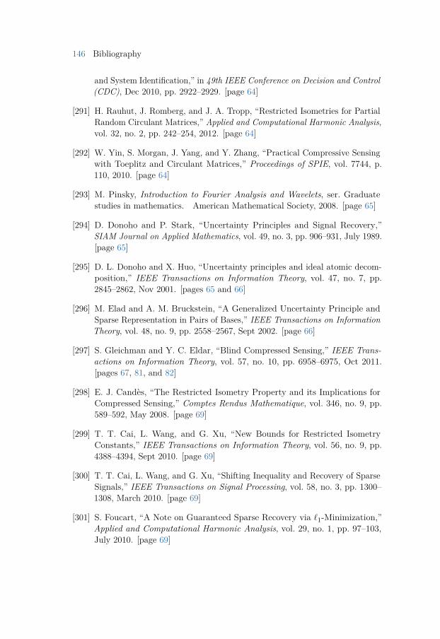
146 Bibliography
and System Identification,” in 49th IEEE Conference on Decision and Control(CDC), Dec 2010, pp. 2922–2929. [page 64]
[291] H. Rauhut, J. Romberg, and J. A. Tropp, “Restricted Isometries for PartialRandom Circulant Matrices,” Applied and Computational Harmonic Analysis,vol. 32, no. 2, pp. 242–254, 2012. [page 64]
[292] W. Yin, S. Morgan, J. Yang, and Y. Zhang, “Practical Compressive Sensingwith Toeplitz and Circulant Matrices,” Proceedings of SPIE, vol. 7744, p.110, 2010. [page 64]
[293] M. Pinsky, Introduction to Fourier Analysis and Wavelets, ser. Graduatestudies in mathematics. American Mathematical Society, 2008. [page 65]
[294] D. Donoho and P. Stark, “Uncertainty Principles and Signal Recovery,”SIAM Journal on Applied Mathematics, vol. 49, no. 3, pp. 906–931, July 1989.[page 65]
[295] D. L. Donoho and X. Huo, “Uncertainty principles and ideal atomic decom-position,” IEEE Transactions on Information Theory, vol. 47, no. 7, pp.2845–2862, Nov 2001. [pages 65 and 66]
[296] M. Elad and A. M. Bruckstein, “A Generalized Uncertainty Principle andSparse Representation in Pairs of Bases,” IEEE Transactions on InformationTheory, vol. 48, no. 9, pp. 2558–2567, Sept 2002. [page 66]
[297] S. Gleichman and Y. C. Eldar, “Blind Compressed Sensing,” IEEE Trans-actions on Information Theory, vol. 57, no. 10, pp. 6958–6975, Oct 2011.[pages 67, 81, and 82]
[298] E. J. Candès, “The Restricted Isometry Property and its Implications forCompressed Sensing,” Comptes Rendus Mathematique, vol. 346, no. 9, pp.589–592, May 2008. [page 69]
[299] T. T. Cai, L. Wang, and G. Xu, “New Bounds for Restricted IsometryConstants,” IEEE Transactions on Information Theory, vol. 56, no. 9, pp.4388–4394, Sept 2010. [page 69]
[300] T. T. Cai, L. Wang, and G. Xu, “Shifting Inequality and Recovery of SparseSignals,” IEEE Transactions on Signal Processing, vol. 58, no. 3, pp. 1300–1308, March 2010. [page 69]
[301] S. Foucart, “A Note on Guaranteed Sparse Recovery via `1-Minimization,”Applied and Computational Harmonic Analysis, vol. 29, no. 1, pp. 97–103,July 2010. [page 69]
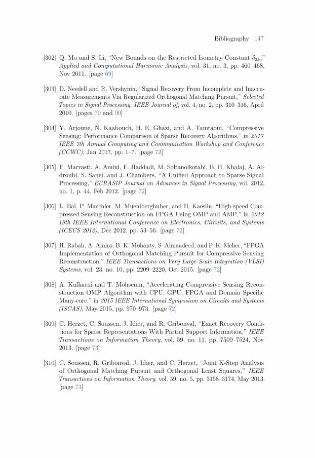
Bibliography 147
[302] Q. Mo and S. Li, “New Bounds on the Restricted Isometry Constant δ2k,”Applied and Computational Harmonic Analysis, vol. 31, no. 3, pp. 460–468,Nov 2011. [page 69]
[303] D. Needell and R. Vershynin, “Signal Recovery From Incomplete and Inaccu-rate Measurements Via Regularized Orthogonal Matching Pursuit,” SelectedTopics in Signal Processing, IEEE Journal of, vol. 4, no. 2, pp. 310–316, April2010. [pages 70 and 90]
[304] Y. Arjoune, N. Kaabouch, H. E. Ghazi, and A. Tamtaoui, “CompressiveSensing: Performance Comparison of Sparse Recovery Algorithms,” in 2017IEEE 7th Annual Computing and Communication Workshop and Conference(CCWC), Jan 2017, pp. 1–7. [page 72]
[305] F. Marvasti, A. Amini, F. Haddadi, M. Soltanolkotabi, B. H. Khalaj, A. Al-droubi, S. Sanei, and J. Chambers, “A Unified Approach to Sparse SignalProcessing,” EURASIP Journal on Advances in Signal Processing, vol. 2012,no. 1, p. 44, Feb 2012. [page 72]
[306] L. Bai, P. Maechler, M. Muehlberghuber, and H. Kaeslin, “High-speed Com-pressed Sensing Reconstruction on FPGA Using OMP and AMP,” in 201219th IEEE International Conference on Electronics, Circuits, and Systems(ICECS 2012), Dec 2012, pp. 53–56. [page 72]
[307] H. Rabah, A. Amira, B. K. Mohanty, S. Almaadeed, and P. K. Meher, “FPGAImplementation of Orthogonal Matching Pursuit for Compressive SensingReconstruction,” IEEE Transactions on Very Large Scale Integration (VLSI)Systems, vol. 23, no. 10, pp. 2209–2220, Oct 2015. [page 72]
[308] A. Kulkarni and T. Mohsenin, “Accelerating Compressive Sensing Recon-struction OMP Algorithm with CPU, GPU, FPGA and Domain SpecificMany-core,” in 2015 IEEE International Symposium on Circuits and Systems(ISCAS), May 2015, pp. 970–973. [page 72]
[309] C. Herzet, C. Soussen, J. Idier, and R. Gribonval, “Exact Recovery Condi-tions for Sparse Representations With Partial Support Information,” IEEETransactions on Information Theory, vol. 59, no. 11, pp. 7509–7524, Nov2013. [page 73]
[310] C. Soussen, R. Gribonval, J. Idier, and C. Herzet, “Joint K-Step Analysisof Orthogonal Matching Pursuit and Orthogonal Least Squares,” IEEETransactions on Information Theory, vol. 59, no. 5, pp. 3158–3174, May 2013.[page 73]
148 Bibliography
[311] Q. Mo and Y. Shen, “A Remark on the Restricted Isometry Property inOrthogonal Matching Pursuit,” IEEE Transactions on Information Theory,vol. 58, no. 6, pp. 3654–3656, June 2012. [page 73]
[312] J. Wang and B. Shim, “On the Recovery Limit of Sparse Signals UsingOrthogonal Matching Pursuit,” IEEE Transactions on Signal Processing,vol. 60, no. 9, pp. 4973–4976, Sept 2012. [page 73]
[313] R. Wu, W. Huang, and D. Chen, “The Exact Support Recovery of Sparse Sig-nals With Noise via Orthogonal Matching Pursuit,” IEEE Signal ProcessingLetters, vol. 20, no. 4, pp. 403–406, April 2013. [page 73]
[314] J. Wen, Z. Zhou, J. Wang, X. Tang, and Q. Mo, “A Sharp Condition for ExactSupport Recovery With Orthogonal Matching Pursuit,” IEEE Transactionson Signal Processing, vol. 65, no. 6, pp. 1370–1382, March 2017. [page 73]
[315] J. Wang and B. Shim, “Exact Recovery of Sparse Signals Using OrthogonalMatching Pursuit: How Many Iterations Do We Need?” IEEE Transactionson Signal Processing, vol. 64, no. 16, pp. 4194–4202, Aug 2016. [page 73]
[316] J. Ding, L. Chen, and Y. Gu, “Perturbation Analysis of Orthogonal MatchingPursuit,” IEEE Transactions on Signal Processing, vol. 61, no. 2, pp. 398–410,Jan 2013. [page 73]
[317] A. M. Tillmann and M. E. Pfetsch, “The computational complexity of therestricted isometry property, the nullspace property, and related conceptsin compressed sensing,” IEEE Transactions on Information Theory, vol. 60,no. 2, pp. 1248–1259, Feb 2014. [page 74]
[318] G. Bennett, “Probability Inequalities for the Sum of Independent RandomVariables,” Journal of the American Statistical Association, vol. 57, no. 297,pp. 33–45, 1962. [page 76]
[319] S. Boucheron, G. Lugosi, and P. Massart, Concentration Inequalities: ANonasymptotic Theory of Independence. OUP Oxford, 2013. [page 76]
[320] J. A. Tropp, “User-Friendly Tail Bounds for Sums of Random Matrices,”Foundations of Computational Mathematics, vol. 12, no. 4, pp. 389–434, Aug2012. [page 83]
[321] C. Luo, F. Wu, J. Sun, and C. W. Chen, “Compressive Data Gathering forLarge-scale Wireless Sensor Networks,” in Proceedings of the 15th Annual In-ternational Conference on Mobile Computing and Networking, ser. MobiCom’09. ACM, 2009, pp. 145–156. [page 89]
Bibliography 149
[322] Z. Tian and G. B. Giannakis, “Compressed Sensing for Wideband Cogni-tive Radios,” in 2007 IEEE International Conference on Acoustics, Speechand Signal Processing, ser. ICASSP ’07, April 2007, pp. IV–1357–IV–1360.[page 89]
[323] P. Nagesh and B. Li, “A Compressive Sensing Approach for Expression-Invariant Face Recognition,” in 2009 IEEE Conference on Computer Visionand Pattern Recognition, June 2009, pp. 1518–1525. [page 89]
[324] J. F. Gemmeke, H. V. Hamme, B. Cranen, and L. Boves, “CompressiveSensing for Missing Data Imputation in Noise Robust Speech Recognition,”IEEE Journal of Selected Topics in Signal Processing, vol. 4, no. 2, pp.272–287, April 2010. [page 89]
[325] A. Akl, C. Feng, and S. Valaee, “A Novel Accelerometer-Based GestureRecognition System,” IEEE Transactions on Signal Processing, vol. 59, no. 12,pp. 6197–6205, Dec 2011. [page 89]
[326] A. Amir and O. Zuk, “Bacterial Community Reconstruction Using Com-pressed Sensing,” Journal of computational biology, vol. 18, no. 11, pp.1723–1741, Nov 2011. [page 89]
[327] W. TANG, H. CAO, J. DUAN, and Y.-P. WANG, “A Compressed SensingBased Approach for subtyping of Leukemia from Gene Expression Data,”Journal of Bioinformatics and Computational Biology, vol. 09, no. 05, pp.631–645, 2011. [page 89]
[328] V. M. Patel, G. R. Easley, J. D. M. Healy, and R. Chellappa, “CompressedSynthetic Aperture Radar,” IEEE Journal of Selected Topics in Signal Pro-cessing, vol. 4, no. 2, pp. 244–254, April 2010. [page 89]
[329] A. C. Gurbuz, J. H. McClellan, and W. R. S. Jr., “Compressive Sensing forSubsurface Imaging Using Ground Penetrating Radar,” Signal Processing,vol. 89, no. 10, pp. 1959–1972, Oct 2009. [page 89]
[330] D. Shamsi, P. Boufounos, and F. Koushanfar, “Noninvasive Leakage PowerTomography of Integrated Circuits by Compressive Sensing,” in Proceedingof the 13th international symposium on Low power electronics and design(ISLPED ’08), Aug 2008, pp. 341–346. [page 89]
[331] D. Gangopadhyay, E. G. Allstot, A. M. R. Dixon, K. Natarajan, S. Gupta,and D. J. Allstot, “Compressed Sensing Analog Front-End for Bio-SensorApplications,” IEEE Journal of Solid-State Circuits, vol. 49, no. 2, pp. 426–438, Feb 2014. [page 89]
150 Bibliography
[332] C. Liao, J. Tao, X. Zeng, Y. Su, D. Zhou, and X. Li, “Efficient SpatialVariation Modeling of Nanoscale Integrated Circuits Via Hidden MarkovTree,” IEEE Transactions on Computer-Aided Design of Integrated Circuitsand Systems, vol. 35, no. 6, pp. 971–984, June 2016. [page 89]
[333] T. Xu and W. Wang, “A Compressed Sensing Approach for Underdeter-mined Blind Audio Source Separation with Sparse Representation,” in 2009IEEE/SP 15th Workshop on Statistical Signal Processing, Aug 2009, pp.493–496. [page 89]
[334] G. Bao, Z. Ye, X. Xu, and Y. Zhou, “A Compressed Sensing Approach toBlind Separation of Speech Mixture Based on a Two-Layer Sparsity Model,”IEEE Transactions on Audio, Speech, and Language Processing, vol. 21, no. 5,pp. 899–906, May 2013. [page 89]
[335] F. M. aes, F. M. Araújo, M. V. Correia, M. Abolbashari, and F. Farahi,“Active Illumination Single-pixel Camera Based on Compressive Sensing,”Applied Optics, vol. 50, no. 4, pp. 405–414, Feb 2011. [page 89]
[336] Z. Li, J. Suo, X. Hu, C. Deng, J. Fan, and Q. Dai, “Efficient Single-pixel Multi-spectral Imaging via Non-mechanical Spatio-spectral Modulation,” ScientificReports, vol. 7, no. 41435, Jan 2017. [page 90]
[337] H. Garcia, C. V. Correa, and H. Arguello, “Multi-Resolution CompressiveSpectral Imaging Reconstruction From Single Pixel Measurements,” IEEETransactions on Image Processing, vol. 27, no. 12, pp. 6174–6184, Dec 2018.[page 90]
[338] M. P. Edgar, G. M. Gibson, R. W. Bowman, B. Sun, N. Radwell, K. J.Mitchell, S. S. Welsh, and M. J. Padgett1, “Simultaneous Real-time Visibleand Infrared Video with Single-pixel Detectors,” Scientific Reports, vol. 5,no. 10669, May 2015. [page 90]
[339] N. Radwell, K. J. Mitchell, G. M. Gibson, M. P. Edgar, R. Bowman, andM. J. Padgett, “Single-pixel Infrared and Visible Microscope,” Optica, vol. 1,no. 5, pp. 285–289, Nov 2014. [page 90]
[340] W. L. Chan, K. Charan, D. Takhar, K. F. Kelly, R. G. Baraniuk, and D. M.Mittleman, “A Single-pixel Terahertz Imaging System Based on CompressedSensing,” Applied Physics Letters, vol. 93, no. 12, p. 121105, Sep 2008.[page 90]
[341] Z. Fang, N. Van Le, M. Choy, and J. H. Lee, “High Spatial ResolutionCompressed Sensing (HSPARSE) Functional MRI,” Magnetic Resonance inMedicine, vol. 76, no. 2, pp. 440–455, Oct 2015. [page 90]
Bibliography 151
[342] W. Lu, T. Li, I. C. Atkinson, and N. Vaswani, “Modified-CS-residual for Re-cursive Reconstruction of Highly Undersampled Functional MRI Sequences,”in 2011 18th IEEE International Conference on Image Processing, Sept 2011,pp. 2689–2692. [page 90]
[343] X. Zong, J. Lee, A. J. Poplawsky, S.-G. Kim, and J. C. Ye, “CompressedSensing fMRI Using Gradient-recalled Echo and EPI Sequences,” NeuroImage,vol. 92, pp. 312–321, May 2014. [page 90]
[344] D. J. Holland, C. Liu, X. Song, E. L. Mazerolle, M. T. Stevens, A. J. Sederman,L. F. Gladden, R. C. N. D’Arcy, C. V. Bowen, and S. D. Beyea, “CompressedSensing Reconstruction Improves Sensitivity of Variable Density Spiral fMRI,”Magnetic Resonance in Medicine, vol. 70, no. 6, pp. 1634–1643, Feb 2013.[page 90]
[345] U. Gamper, P. Boesiger, and S. Kozerke, “Compressed Sensing in DynamicMRI,” Magnetic Resonance in Medicine, vol. 59, no. 2, pp. 365–373, Jan2008. [page 90]
[346] C. Qiu, W. Lu, and N. Vaswani, “Real-time Dynamic MR Image Reconstruc-tion Using Kalman Filtered Compressed Sensing,” in 2009 IEEE InternationalConference on Acoustics, Speech and Signal Processing, April 2009, pp. 393–396. [page 90]
[347] R. Otazo, E. Candès, and D. K. Sodickson, “Low-rank Plus Sparse MatrixDecomposition for Accelerated Dynamic MRI with Separation of Backgroundand Dynamic Components,” Magnetic Resonance in Medicine, vol. 73, no. 3,pp. 1125–1136, April 2014. [page 90]
[348] L. Feng, R. Grimm, K. T. Block, H. Chandarana, S. Kim, J. Xu, L. Axel,D. K. Sodickson, and R. Otazo, “Golden-angle Radial Sparse Parallel MRI:Combination of Compressed Sensing, Parallel Imaging, and Golden-angleRadial Sampling for Fast and Flexible Dynamic Volumetric MRI,” MagneticResonance in Medicine, vol. 72, no. 3, pp. 707–717, Oct 2013. [page 90]
[349] H. Haji-Valizadeh, A. A. Rahsepar, J. D. Collins, E. Bassett, T. Isakova,T. Block, G. Adluru, E. V. R. DiBella, D. C. Lee, J. C. Carr, and D. Kim,“Validation of Highly Accelerated Real-time Cardiac Cine MRI with RadialK-space Sampling and Compressed Sensing in Patients at 1.5T and 3T,”Magnetic Resonance in Medicine, vol. 79, no. 5, pp. 2745–2751, Sep 2017.[page 90]
[350] N. Vaswani and J. Zhan, “Recursive Recovery of Sparse Signal SequencesFrom Compressive Measurements: A Review,” IEEE Transactions on SignalProcessing, vol. 64, no. 13, pp. 3523–3549, July 2016. [page 90]
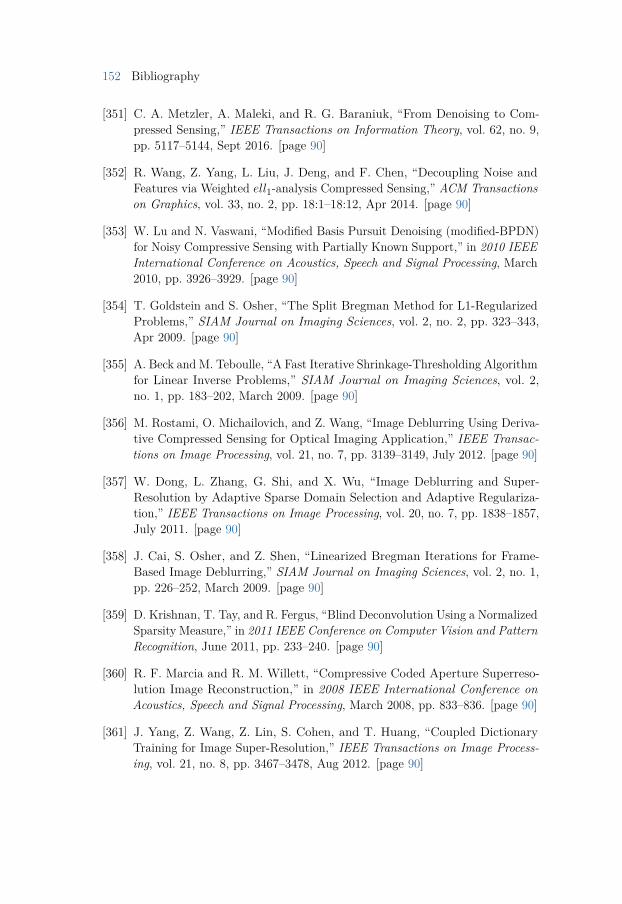
152 Bibliography
[351] C. A. Metzler, A. Maleki, and R. G. Baraniuk, “From Denoising to Com-pressed Sensing,” IEEE Transactions on Information Theory, vol. 62, no. 9,pp. 5117–5144, Sept 2016. [page 90]
[352] R. Wang, Z. Yang, L. Liu, J. Deng, and F. Chen, “Decoupling Noise andFeatures via Weighted ell1-analysis Compressed Sensing,” ACM Transactionson Graphics, vol. 33, no. 2, pp. 18:1–18:12, Apr 2014. [page 90]
[353] W. Lu and N. Vaswani, “Modified Basis Pursuit Denoising (modified-BPDN)for Noisy Compressive Sensing with Partially Known Support,” in 2010 IEEEInternational Conference on Acoustics, Speech and Signal Processing, March2010, pp. 3926–3929. [page 90]
[354] T. Goldstein and S. Osher, “The Split Bregman Method for L1-RegularizedProblems,” SIAM Journal on Imaging Sciences, vol. 2, no. 2, pp. 323–343,Apr 2009. [page 90]
[355] A. Beck and M. Teboulle, “A Fast Iterative Shrinkage-Thresholding Algorithmfor Linear Inverse Problems,” SIAM Journal on Imaging Sciences, vol. 2,no. 1, pp. 183–202, March 2009. [page 90]
[356] M. Rostami, O. Michailovich, and Z. Wang, “Image Deblurring Using Deriva-tive Compressed Sensing for Optical Imaging Application,” IEEE Transac-tions on Image Processing, vol. 21, no. 7, pp. 3139–3149, July 2012. [page 90]
[357] W. Dong, L. Zhang, G. Shi, and X. Wu, “Image Deblurring and Super-Resolution by Adaptive Sparse Domain Selection and Adaptive Regulariza-tion,” IEEE Transactions on Image Processing, vol. 20, no. 7, pp. 1838–1857,July 2011. [page 90]
[358] J. Cai, S. Osher, and Z. Shen, “Linearized Bregman Iterations for Frame-Based Image Deblurring,” SIAM Journal on Imaging Sciences, vol. 2, no. 1,pp. 226–252, March 2009. [page 90]
[359] D. Krishnan, T. Tay, and R. Fergus, “Blind Deconvolution Using a NormalizedSparsity Measure,” in 2011 IEEE Conference on Computer Vision and PatternRecognition, June 2011, pp. 233–240. [page 90]
[360] R. F. Marcia and R. M. Willett, “Compressive Coded Aperture Superreso-lution Image Reconstruction,” in 2008 IEEE International Conference onAcoustics, Speech and Signal Processing, March 2008, pp. 833–836. [page 90]
[361] J. Yang, Z. Wang, Z. Lin, S. Cohen, and T. Huang, “Coupled DictionaryTraining for Image Super-Resolution,” IEEE Transactions on Image Process-ing, vol. 21, no. 8, pp. 3467–3478, Aug 2012. [page 90]

Bibliography 153
[362] Y. Rivenson, A. Stern, and B. Javidi, “Single Exposure Super-resolutionCompressive Imaging by Double Phase Encoding,” Optics Express, vol. 18,no. 14, pp. 15 094–15 103, Jul 2010. [page 90]
[363] X. Gao, K. Zhang, D. Tao, and X. Li, “Image Super-Resolution With SparseNeighbor Embedding,” IEEE Transactions on Image Processing, vol. 21,no. 7, pp. 3194–3205, July 2012. [page 90]
[364] M. Hirsch, G. Wetzstein, and R. Raskar, “A Compressive Light Field Projec-tion System,” ACM Transactions on Graphics, vol. 33, no. 4, pp. 58:1–58:12,Jul 2014. [page 90]
[365] A. Maimone, G. Wetzstein, M. Hirsch, D. Lanman, R. Raskar, and H. Fuchs,“Focus 3D: Compressive Accommodation Display,” ACM Transactions onGraphics, vol. 32, no. 5, pp. 153:1–153:13, Oct 2013. [page 90]
[366] Y. Huo, R. Wang, S. Jin, X. Liu, and H. Bao, “A Matrix Sampling-and-recovery Approach for Many-lights Rendering,” ACM Transactions on Graph-ics, vol. 34, no. 6, pp. 210:1–210:12, Oct 2015. [page 90]
[367] B. Wilburn, N. Joshi, V. Vaish, E.-V. Talvala, E. Antunez, A. Barth,A. Adams, M. Horowitz, and M. Levoy, “High Performance Imaging Us-ing Large Camera Arrays,” ACM Transactions on Graphics, vol. 24, no. 3,pp. 765–776, Jul 2005. [pages 91 and 92]
[368] J. Unger, A. Wenger, T. Hawkins, A. Gardner, and P. Debevec, “Captur-ing and Rendering with Incident Light Fields,” in Proceedings of the 14thEurographics Workshop on Rendering. Eurographics Association, 2003, pp.141–149. [page 92]
[369] M. Hirsch, S. Sivaramakrishnan, S. Jayasuriya, A. Wang, A. Molnar,R. Raskar, and G. Wetzstein, “A switchable Light Field Camera Archi-tecture with Angle Sensitive Pixels and Dictionary-based Sparse Coding,” in2014 IEEE International Conference on Computational Photography (ICCP),May 2014, pp. 1–10. [pages 92 and 93]
[370] M. Levoy and P. Hanrahan, “Light Field Rendering,” in Proceedings ofSIGGRAPH 1996. ACM, 1996, pp. 31–42. [page 92]
[371] J. Unger, S. Gustavson, P. Larsson, and A. Ynnerman, “Free Form IncidentLight Fields,” in Proceedings of the Nineteenth Eurographics Conference onRendering, ser. EGSR ’08. Eurographics Association, 2008, pp. 1293–1301.[page 92]
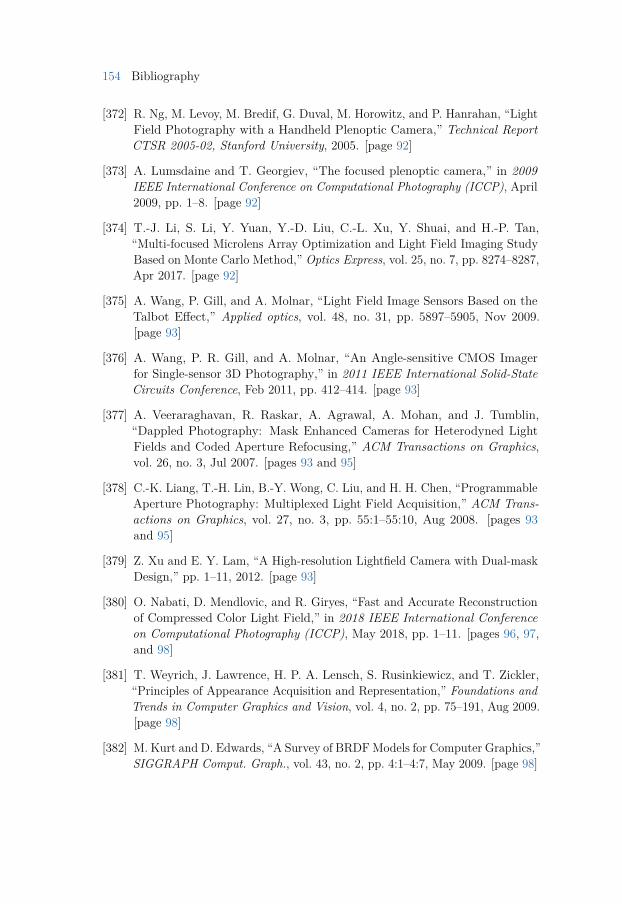
154 Bibliography
[372] R. Ng, M. Levoy, M. Bredif, G. Duval, M. Horowitz, and P. Hanrahan, “LightField Photography with a Handheld Plenoptic Camera,” Technical ReportCTSR 2005-02, Stanford University, 2005. [page 92]
[373] A. Lumsdaine and T. Georgiev, “The focused plenoptic camera,” in 2009IEEE International Conference on Computational Photography (ICCP), April2009, pp. 1–8. [page 92]
[374] T.-J. Li, S. Li, Y. Yuan, Y.-D. Liu, C.-L. Xu, Y. Shuai, and H.-P. Tan,“Multi-focused Microlens Array Optimization and Light Field Imaging StudyBased on Monte Carlo Method,” Optics Express, vol. 25, no. 7, pp. 8274–8287,Apr 2017. [page 92]
[375] A. Wang, P. Gill, and A. Molnar, “Light Field Image Sensors Based on theTalbot Effect,” Applied optics, vol. 48, no. 31, pp. 5897–5905, Nov 2009.[page 93]
[376] A. Wang, P. R. Gill, and A. Molnar, “An Angle-sensitive CMOS Imagerfor Single-sensor 3D Photography,” in 2011 IEEE International Solid-StateCircuits Conference, Feb 2011, pp. 412–414. [page 93]
[377] A. Veeraraghavan, R. Raskar, A. Agrawal, A. Mohan, and J. Tumblin,“Dappled Photography: Mask Enhanced Cameras for Heterodyned LightFields and Coded Aperture Refocusing,” ACM Transactions on Graphics,vol. 26, no. 3, Jul 2007. [pages 93 and 95]
[378] C.-K. Liang, T.-H. Lin, B.-Y. Wong, C. Liu, and H. H. Chen, “ProgrammableAperture Photography: Multiplexed Light Field Acquisition,” ACM Trans-actions on Graphics, vol. 27, no. 3, pp. 55:1–55:10, Aug 2008. [pages 93and 95]
[379] Z. Xu and E. Y. Lam, “A High-resolution Lightfield Camera with Dual-maskDesign,” pp. 1–11, 2012. [page 93]
[380] O. Nabati, D. Mendlovic, and R. Giryes, “Fast and Accurate Reconstructionof Compressed Color Light Field,” in 2018 IEEE International Conferenceon Computational Photography (ICCP), May 2018, pp. 1–11. [pages 96, 97,and 98]
[381] T. Weyrich, J. Lawrence, H. P. A. Lensch, S. Rusinkiewicz, and T. Zickler,“Principles of Appearance Acquisition and Representation,” Foundations andTrends in Computer Graphics and Vision, vol. 4, no. 2, pp. 75–191, Aug 2009.[page 98]
[382] M. Kurt and D. Edwards, “A Survey of BRDFModels for Computer Graphics,”SIGGRAPH Comput. Graph., vol. 43, no. 2, pp. 4:1–4:7, May 2009. [page 98]
Bibliography 155
[383] E. Veach and L. Guibas, “Bidirectional Estimators for Light Transport,” inPhotorealistic Rendering Techniques. Springer Berlin Heidelberg, 1995, pp.145–167. [page 98]
[384] S. Popov, R. Ramamoorthi, F. Durand, and G. Drettakis, “ProbabilisticConnections for Bidirectional Path Tracing,” in Proceedings of the 26th Euro-graphics Symposium on Rendering, ser. EGSR ’15. Eurographics Association,2015, pp. 75–86. [page 98]
[385] H. W. Jensen, “Global Illumination Using Photon Maps,” in Proceedings ofthe Eurographics Workshop on Rendering Techniques ’96. Springer-Verlag,1996, pp. 21–30. [page 98]
[386] A. S. Kaplanyan and C. Dachsbacher, “Adaptive Progressive Photon Map-ping,” ACM Transactions on Graphics, vol. 32, no. 2, pp. 16:1–16:13, Apr2013. [page 98]
[387] H. Qin, X. Sun, Q. Hou, B. Guo, and K. Zhou, “Unbiased Photon Gatheringfor Light Transport Simulation,” ACM Transactions on Graphics, vol. 34,no. 6, pp. 208:1–208:14, Oct 2015. [page 98]
[388] E. Veach and L. J. Guibas, “Metropolis Light Transport,” in Proceedingsof the 24th Annual Conference on Computer Graphics and Interactive Tech-niques (SIGGRAPH ’97). ACM Press/Addison-Wesley Publishing Co., 1997.[page 98]
[389] T.-M. Li, J. Lehtinen, R. Ramamoorthi, W. Jakob, and F. Durand,“Anisotropic Gaussian Mutations for Metropolis Light Transport ThroughHessian-Hamiltonian Dynamics,” ACM Transactions on Graphics, vol. 34,no. 6, pp. 209:1–209:13, Oct 2015. [page 98]
[390] M. Manzi, F. Rousselle, M. Kettunen, J. Lehtinen, and M. Zwicker, “Im-proved Sampling for Gradient-domain Metropolis Light Transport,” ACMTransactions on Graphics, vol. 33, no. 6, pp. 178:1–178:12, Nov 2014. [page 98]
[391] J. Pantaleoni, “Charted Metropolis Light Transport,” ACM Transactions onGraphics, vol. 36, no. 4, pp. 75:1–75:14, Jul 2017. [page 98]
[392] M. Zwicker, W. Jarosz, J. Lehtinen, B. Moon, R. Ramamoorthi, F. Rousselle,P. Sen, C. Soler, and S.-E. Yoon, “Recent Advances in Adaptive Samplingand Reconstruction for Monte Carlo Rendering,” Computer Graphics Forum,vol. 34, no. 2, pp. 667–681, June 2015. [page 98]
[393] P. Bauszat, M. Eisemann, and M. Magnor, “Guided Image Filtering forInteractive High-quality Global Illumination,” Computer Graphics Forum,vol. 30, no. 4, pp. 1361–1368, July 2011. [page 98]
156 Bibliography
[394] B. Moon, J. Y. Jun, J. Lee, K. Kim, T. Hachisuka, and S.-E. Yoon, “RobustImage Denoising Using a Virtual Flash Image for Monte Carlo Ray Tracing,”Computer Graphics Forum, vol. 32, no. 1, pp. 139–151, July 2013. [page 98]
[395] F. Rousselle, C. Knaus, and M. Zwicker, “Adaptive Rendering with Non-local Means Filtering,” ACM Transactions on Graphics, vol. 31, no. 6, pp.195:1–195:11, Nov 2012. [page 98]
[396] M. Delbracio, P. Musé, A. Buades, J. Chauvier, N. Phelps, and J.-M. Morel,“Boosting Monte Carlo Rendering by Ray Histogram Fusion,” ACM Transac-tions on Graphics, vol. 33, no. 1, pp. 8:1–8:15, Feb 2014. [page 98]
[397] S. Bako, T. Vogels, B. Mcwilliams, M. Meyer, J. NováK, A. Harvill, P. Sen,T. Derose, and F. Rousselle, “Kernel-predicting Convolutional Networks forDenoising Monte Carlo Renderings,” ACM Transactions on Graphics, vol. 36,no. 4, pp. 97:1–97:14, Jul 2017. [page 98]
[398] P. Sen and S. Darabi, “Compressive Rendering: A Rendering Application ofCompressed Sensing,” IEEE Transactions on Visualization and ComputerGraphics, vol. 17, no. 4, pp. 487–499, Apr 2011. [pages 99, 101, and 102]
[399] B. Choudhury, R. Swanson, F. Heide, G. Wetzstein, and W. Heidrich, “Con-sensus Convolutional Sparse Coding,” in 2017 IEEE International Conferenceon Computer Vision (ICCV), Oct 2017, pp. 4290–4298. [page 102]
[400] J. Liu, P. Musialski, P. Wonka, and J. Ye, “Tensor Completion for EstimatingMissing Values in Visual Data,” IEEE Transactions on Pattern Analysis andMachine Intelligence, vol. 35, no. 1, pp. 208–220, Jan 2013. [page 102]
[401] H. Takeda, S. Farsiu, and P. Milanfar, “Kernel Regression for Image Process-ing and Reconstruction,” IEEE Transactions on Image Processing, vol. 16,no. 2, pp. 349–366, Feb 2007. [page 102]
[402] G. Yu, G. Sapiro, and S. Mallat, “Solving Inverse Problems With PiecewiseLinear Estimators: From Gaussian Mixture Models to Structured Sparsity,”IEEE Transactions on Image Processing, vol. 21, no. 5, pp. 2481–2499, May2012. [page 102]
[403] M. Zhou, H. Chen, J. Paisley, L. Ren, L. Li, Z. Xing, D. Dunson, G. Sapiro,and L. Carin, “Nonparametric Bayesian Dictionary Learning for Analysisof Noisy and Incomplete Images,” IEEE Transactions on Image Processing,vol. 21, no. 1, pp. 130–144, Jan 2012. [page 102]
[404] M. D. Zeiler, D. Krishnan, G. W. Taylor, and R. Fergus, “DeconvolutionalNetworks,” in 2010 IEEE Computer Society Conference on Computer Visionand Pattern Recognition, June 2010, pp. 2528–2535. [page 102]
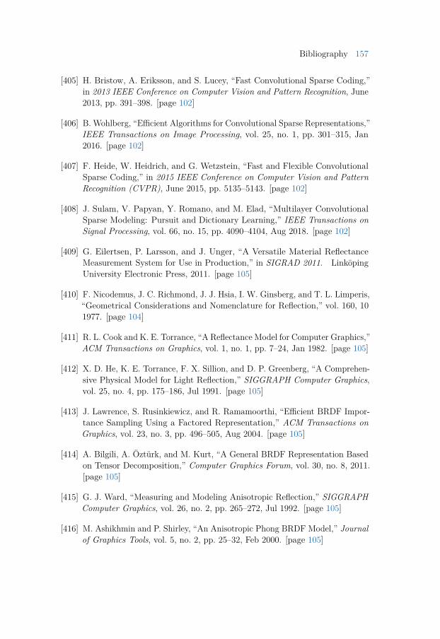
Bibliography 157
[405] H. Bristow, A. Eriksson, and S. Lucey, “Fast Convolutional Sparse Coding,”in 2013 IEEE Conference on Computer Vision and Pattern Recognition, June2013, pp. 391–398. [page 102]
[406] B. Wohlberg, “Efficient Algorithms for Convolutional Sparse Representations,”IEEE Transactions on Image Processing, vol. 25, no. 1, pp. 301–315, Jan2016. [page 102]
[407] F. Heide, W. Heidrich, and G. Wetzstein, “Fast and Flexible ConvolutionalSparse Coding,” in 2015 IEEE Conference on Computer Vision and PatternRecognition (CVPR), June 2015, pp. 5135–5143. [page 102]
[408] J. Sulam, V. Papyan, Y. Romano, and M. Elad, “Multilayer ConvolutionalSparse Modeling: Pursuit and Dictionary Learning,” IEEE Transactions onSignal Processing, vol. 66, no. 15, pp. 4090–4104, Aug 2018. [page 102]
[409] G. Eilertsen, P. Larsson, and J. Unger, “A Versatile Material ReflectanceMeasurement System for Use in Production,” in SIGRAD 2011. LinköpingUniversity Electronic Press, 2011. [page 105]
[410] F. Nicodemus, J. C. Richmond, J. J. Hsia, I. W. Ginsberg, and T. L. Limperis,“Geometrical Considerations and Nomenclature for Reflection,” vol. 160, 101977. [page 104]
[411] R. L. Cook and K. E. Torrance, “A Reflectance Model for Computer Graphics,”ACM Transactions on Graphics, vol. 1, no. 1, pp. 7–24, Jan 1982. [page 105]
[412] X. D. He, K. E. Torrance, F. X. Sillion, and D. P. Greenberg, “A Comprehen-sive Physical Model for Light Reflection,” SIGGRAPH Computer Graphics,vol. 25, no. 4, pp. 175–186, Jul 1991. [page 105]
[413] J. Lawrence, S. Rusinkiewicz, and R. Ramamoorthi, “Efficient BRDF Impor-tance Sampling Using a Factored Representation,” ACM Transactions onGraphics, vol. 23, no. 3, pp. 496–505, Aug 2004. [page 105]
[414] A. Bilgili, A. Öztürk, and M. Kurt, “A General BRDF Representation Basedon Tensor Decomposition,” Computer Graphics Forum, vol. 30, no. 8, 2011.[page 105]
[415] G. J. Ward, “Measuring and Modeling Anisotropic Reflection,” SIGGRAPHComputer Graphics, vol. 26, no. 2, pp. 265–272, Jul 1992. [page 105]
[416] M. Ashikhmin and P. Shirley, “An Anisotropic Phong BRDF Model,” Journalof Graphics Tools, vol. 5, no. 2, pp. 25–32, Feb 2000. [page 105]
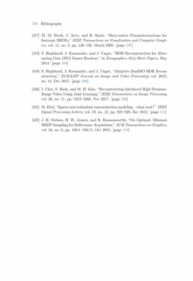
158 Bibliography
[417] M. M. Stark, J. Arvo, and B. Smits, “Barycentric Parameterizations forIsotropic BRDFs,” IEEE Transactions on Visualization and Computer Graph-ics, vol. 11, no. 2, pp. 126–138, March 2005. [page 107]
[418] S. Hajisharif, J. Kronander, and J. Unger, “HDR Reconstruction for Alter-nating Gain (ISO) Sensor Readout,” in Eurographics 2014 Short Papers, May2014. [page 108]
[419] S. Hajisharif, J. Kronander, and J. Unger, “Adaptive DualISO HDR Recon-struction,” EURASIP Journal on Image and Video Processing, vol. 2015,no. 41, Dec 2015. [page 108]
[420] I. Choi, S. Baek, and M. H. Kim, “Reconstructing Interlaced High-Dynamic-Range Video Using Joint Learning,” IEEE Transactions on Image Processing,vol. 26, no. 11, pp. 5353–5366, Nov 2017. [page 108]
[421] M. Elad, “Sparse and redundant representation modeling—what next?” IEEESignal Processing Letters, vol. 19, no. 12, pp. 922–928, Dec 2012. [page 111]
[422] J. B. Nielsen, H. W. Jensen, and R. Ramamoorthi, “On Optimal, MinimalBRDF Sampling for Reflectance Acquisition,” ACM Transactions on Graphics,vol. 34, no. 6, pp. 186:1–186:11, Oct 2015. [page 116]

Publications
The publications associated with this thesis have been removed for copyright reasons. For more details about these see:
http://urn.kb.se/resolve?urn=urn:nbn:se:liu:diva-152863