Sd(

Ja

b

a

A

R

R

1

A

P

K

I

F

P

E

1

SiuaCtr(1ar

O

0d

e c o l o g i c a l m o d e l l i n g 2 1 3 ( 2 0 0 8 ) 33–44

avai lab le at www.sc iencedi rec t .com

journa l homepage: www.e lsev ier .com/ locate /eco lmodel

imulation model of universal law of school sizeistribution applied to southern bluefin tuna

Thunnus maccoyii) in the Great Australian Bight

ay Willisa,b,∗

CSIRO Marine and Atmospheric Research, Castray Esplanade, Hobart, Tasmania 7000, AustraliaSchool of Zoology and Quantitative Marine Science, University of Tasmania, Australia

r t i c l e i n f o

rticle history:

eceived 27 August 2007

eceived in revised form

0 January 2008

ccepted 15 January 2008

ublished on line 5 March 2008

eywords:

ndividual-based model

a b s t r a c t

A universal law of animal group size distribution correlates well to observed fish school size

distribution from fisheries catch data. I applied the law to fisheries independent aerial survey

data of southern bluefin tuna (Thunnus maccoyii) collected over a 10-year period in the Great

Australian Bight. The law does not correlate to the observed school size distribution. A com-

puter model originally demonstrated the formation of the universal law from simple rules.

I redesigned this model as an individual-based simulation model calibrated from acoustic

tag observations and state a mathematical formula for a resultant new family of transient

group size distributions. The new formula correlates accurately to the simulation and to the

aerial survey data. I use the mathematical model to estimate area of aggregation and total

ractal dimension

elagic schooling

mpirical function

abundance. This approach is new as it does not seek stationary states of group size distribu-

tion and because it demonstrates a quantitative relationship between individual behaviour

and group size distribution. This work elevates the pattern of group size distribution from

a curiosity to a useful tool, and introduces a new family of transient distributions that may

have a general application to other grouping phenomena.

throughout their lives (Petitgas et al., 2001). In this study I use

. Introduction

chooling is common behaviour for the majority of fishes dur-ng at least one stage of their life history (Partridge, 1982). Thebiquity of the behaviour suggests that there is an evolution-ry advantage to school membership (Clark and Mangel, 1986;amazine et al., 2003; Ruxton et al., 2005). Structure and func-

ion of fish schools has been understood more deeply afterecent theoretical advances using individual-based modelsAoki, 1982; Warburton and Lazarus, 1991; Huth and Wissel,

992). Despite these studies, still relatively little is knownbout the way schools form, why they disperse, and whatelationship there may be between school size and relative

∗ Correspondingauthorat: Departments of Zoology and Engineering Scxford, OX1 3PS, UK. Tel.: +44 1865 283 154.

E-mail address: jay@robots.ox.ac.uk.304-3800/$ – see front matter © 2008 Elsevier B.V. All rights reserved.oi:10.1016/j.ecolmodel.2008.01.017

© 2008 Elsevier B.V. All rights reserved.

advantage of membership. If there are variable evolutionaryadvantages to be gained from membership of a range of differ-ent sized schools, school size distribution would relate directlyto ecosystem health and function and fish population viability(Petitgas et al., 2001). Indeed the effect of spatial organisationon interaction rates is one of the most important unresolvedchallenges for ecosystem modellers (Fulton et al., 2003).

Tuna provide a good potential example of schoolingbehaviour as they form visible surface schools of various sizes

ience, Oxford University, Tinbergen Building, South Parks Road,

aerial observations of southern bluefin tuna (Thunnus maccoyii)(SBT) schools, which were collected in a scientific survey overthe Great Australian Bight (GAB) during a period of 10 years

l i n g 2 1 3 ( 2 0 0 8 ) 33–44

Fig. 1 – Log–log plot of frequency distribution of aerialsurvey observations of southern bluefin tuna (Thunnusmaccoyii) schools for all years combined (stars). The datahas been binned and normalised, with bins of size 1 tonneunder 10 tonnes, 10 under 100 tonnes and thereafter100 tonnes. Universal law of fish size distribution has beenfitted (blue line). Note the poor fit of the data to theuniversal law in the region of smaller school observation.(For interpretation of the references to colour in this figurelegend, the reader is referred to the web version of the

34 e c o l o g i c a l m o d e l

as part of the southern bluefin tuna recruitment monitoringprogram (Basson et al., 2005).

Bonabeau and Dagorn (1995) suggested a universal law forfish school size distribution that may also describe other nat-ural group distributions. The foundation of their law, a powerlaw, was derived from a computer model (Takayasu, 1989).They refined the power law by including a term for breakup of groups over a certain critical size and re-injection ofmembers into the system as individuals (or minimum sizedgroups—atomic units). Thus, the universal law is a power lawtruncated by an exponential decay. This law shows remarkablecorrelation with tuna school size distribution from fisheriescatch data, across a number of species and fisheries, andshows correlation to other animal grouping (Bonabeau andDagorn, 1995; Bonabeau et al., 1999).

While this potential correlation to a power law is inter-esting, it has been put to little practical use in the 10 yearssince it was identified. In a similar way to many otherpower laws observed in nature (Utsu et al., 1995; Bak, 1997;Manrubia et al., 1999; Sole et al., 1999; Camacho and Sole,2001; Turcotte and Malamud, 2004), this power law may holdlittle or no value other than as a curiosity of nature. Forinstance if the correlation was exact, it would be valuableto infer causal relationships from school size distribution,such as over what time or space scales the groups haveformed.

The simple computer model originally described byTakayasu (1989) offers a potential reason (set of rules) for thepower law. However, there are limitations when it is appliedto observations of fish. What does it mean when observa-tions do not correlate to the power law? When I applied theuniversal law of school size distribution to aerial survey obser-vations the results were inconclusive. The power law appearsto partially fit the data, but there are areas where it system-atically does not fit, in a way that suggests that the basic lawis inadequate rather than that the measurement error is high(Fig. 1).

In this study I replicate the universal law with a simulationmodel that is consistent with individual tuna movement, andwhich can be calibrated against field observations. The aimis to extend the original model, used in the formulation ofthe universal law, as an individual-based simulation and usethis to develop and test a mathematical model for school sizedistribution. The method builds on previous work and demon-strates a direct linkage between individual-based behaviourand a mathematical model of aggregate behaviour. Such amathematical model, derived from first principles, has valueas an empirical function for spatial organisation for ecosys-tem models, and can be used to analyse field observations.The approach enables prediction, highlights causal links andhelps plan fieldwork.

The computer model used by Bonabeau and Dagorn (1995)to explain the power law section of the universal law employsa regular grid. Each grid point is a site which contains a groupof one or more individuals. At each time step the contentsof every site move to a randomly selected new position on

the grid. If two or more groups converge at the same sitethey join together and stay together as a group for all sub-sequent moves. The model, when initiated with a group ofone at each site and without the injection of new individu-

article).

als, progresses from many groups of one to a single groupcontaining all the individuals. This situation without the injec-tion of new individuals was described as the trivial defaultcase (Takayasu, 1989)—many groups of one aggregating to onegroup of many.

If new singletons are injected into the model, for instance,by injecting a new individual to every site at each time step, thefrequency distribution of group sizes forms a stationary powerlaw of exponent approximately −1.5. That is, the relationshipbetween the number of groups of a particular size (n(s)) andthe size of the group (s) is of the form n(s) = ks˛, where ˛ is theexponent and k is a constant. Once the power law is acceptedit can be manipulated and augmented to suggest refinement– for instance splitting and re-injection in which groups breakup into individuals when they reach a certain critical size – aswas suggested by Bonabeau and Dagorn (1995).

Bonabeau and Dagorn (1995) suggested that the grid modelis suitable for simulating tuna movements. Its main limita-tion is that it is dimensionless; one-step random movementfrom any site to any other makes it a ‘mean-field’ abstrac-tion. Physical dimension is required to compare the modelwith observed movements of fish. One refinement is to limitthe random movement to adjacent sites, thus the groups‘walk’ around the grid from local site to site. Such a ran-dom walk can be compared with field observations. Anotherrefinement is to define an interactive distance (d) consistent

with the presumed sensory ability of the tuna. The logi-cal extension of these approaches is the simulation modelpresented here. Simplicity is lost and traded for biological rel-evance.

n g

2

2

Hp(taiciu

2Tbdisl

2TTswe

wostpw(o

vwtvvbarp(smtfoiwemat

e c o l o g i c a l m o d e l l i

. Method

.1. Simulation model

ere the simulation model is described using the standardrotocol suggested for describing individual-based models

Grimm et al., 2006). The protocol is called ODD which refers tohree components of the protocol (overview, design concepts,nd details). The three components of ODD are subdividednto seven elements: purpose, state variables and scales, pro-ess overview and scheduling, design concepts, initialisation,nput, and submodels. The simulation model is describedsing these elements as follows.

.1.1. Purposehe simulation model was constructed to explore the distri-ution of school sizes in the most general conditions. It wasesigned to replicate previous mean-field dimensionless stud-

es in two dimensions and to extend them. The purpose was toimulate a variety of school size frequency distributions andink these to behavioural rules.

.1.2. State variables and scaleshe model encapsulated the two core causal rules of theakayasu (1989) grid model: (1) all individuals or groups moveimilarly across the whole space, and (2) they always join whenithin the interactive distance. The simulation model had two

ntities: (1) an arena and (2) a fish group object.The first entity, the arena, was a two dimensional space in

hich model tuna moved. The position of a tuna (or groupf tuna) was represented by a dimensionless point in thispace. The area was wrapped to create a continuous space;hat is, if tuna moved out of the area to the left (top) they reap-eared again on the right (bottom). The model was designedith no fixed scale. The area was specified in model units

1000 × 1000) to double (16 decimal place) precision and wastherwise unstructured and continuous.

The second model entity was the fish group object (an indi-idual fish was a group of size one). The states of fish groupsere described by size (number of individuals in group), posi-

ion (in two dimensions), direction, speed, and turning angleariation. The random walk of the tuna was defined by twoariables; speed and turning angle variation which has longeen a common way to simulate animal movement (Fraenkelnd Gunn, 1940; Codling, 2007). This movement is called a cor-elated random walk (CRW) (Turchin, 1998) and can cause theath to vary between a straight line and a fully random walk

i.e. one with a randomly chosen direction at each step). Thepeed was the distance moved at each step (default was 20odel units) and the turning angle variation defined the tor-

uosity of the movement (default was a new angle selectedrom a normal random distribution with a standard deviationf 36◦). All fish groups that were used in scenarios explored

n this study had similar values for speed and tortuosity andere thus differentiated only by their position and direction at

ach step. These objects had a single behaviour other than toove in a way described above. The behaviour was to join with

ny other fish group to produce a combined fish group if thewo groups moved to within the interactive distance of each

2 1 3 ( 2 0 0 8 ) 33–44 35

other (default was 10 model units). The new combined fishgroup had similar state and behaviour to one of the groups thatjoined with the exception of a new size equal to the combinedsizes of the component fish group objects.

2.1.3. Process overview and schedulingIf a tuna was within the interactive distance (d) of any other,they joined together and continued in the new group in thesame way as before. Interactive distance was set as half thedistance moved at each time step which is consistent withmoving one grid square at a time in Takayasu (1989) model. Ateach time step every tuna moved, after all moves were com-pleted, each tuna checked for proximity of others, thus thefunctions were scheduled as follows: (1) move (all tuna syn-chronously), (2) join (as determined by positions of all groups),and (3) report statistics. These functions are described in moredetail in the following section.

2.1.4. Design conceptsThis section of ODD (the standard protocol for describingindividual-based models) includes a checklist to be followedwhen designing or describing a model. Three of these checklistitems applicable to the simulation model are as follows:

• Sensing: the model implies that one group object can sensethe presence of another, if there are closer together thanthe interactive distance, and thus form a combined group.The implication is that an individual tuna has the sensorycapacity to remain part of a school and join with a school ifit is within the interactive distance.

• Interaction: interaction is limited to formation of groups asdescribed above.

• Collectives: individuals are grouped as described above.

2.1.5. InitialisationTuna were added to the model by placing them at randomlyselected points and giving them randomly selected initialdirections (default was 10,000 groups of size one to start). Tor-tuosity of southern bluefin tuna (T. maccoyii) SBT was calibratedin an approximately scale-free way by using observations ofSBT in the same area in which the aerial survey had beenmade. Between 1992 and 1994 SBT were studied using ultra-sound telemetry (Davis and Stanley, 2002) for up to 48 h.Tortuosity was calibrated by matching the fractal dimension(D) (Mandelbrot, 1967) of the observed tracks using dividerlengths between 3 and 30 km. In this divider range the log–logplot of divider size against path length (arc/chord ratio) waswell approximated by a straight line leading to a meaningfulvalue for D (R2 = 0.9985, p < 0.0001, D = 1.0858) (Turchin, 1998;Nams, 2006). CRWs have an log–log arc/chord gradient thatvaries between 1 (for scale much less that step length) and 2(for infinitely large scale), but D can have a meaningful valueat medium scales which has been used in track analysis (Fritzet al., 2003). The model was calibrated with a new angle ateach step, chosen from a normal random distribution of angleswith a standard deviation of 36◦ (10% of maximum) (mean

R2 = 0.9989, standard deviation D = 0.0298, mean D = 1.0765, 20replicates). Therefore tortuosity, caused by this parametervalue, matched the observed fractal dimension and was usedthroughout the simulation. The simulation was not sensitive

l i n g

36 e c o l o g i c a l m o d e l

to tortuosity of path, variation of which is mentioned in thediscussion Section 6 of this paper.

2.1.6. InputThe input section of ODD relates to data that is included intothe model from outside sources such as environmental data.This model has no input in this sense.

2.1.7. SubmodelsThere were three submodels: (1) move, (2) join, and (3) mea-sure. (1) The move submodel was a synchronous processwhere each group was moved independently according to therules for the CRW explained above and which were the samefor all groups. (2) The join submodel involved a sequential(asynchronous) process where each group was examined asthe focal group in turn. The focal group was examined in rela-tion to all other existing groups and any that were within theattractive distance were erased and their contents added tothe focal group. (3) The final submodel was the measurementstage when the numbers of groups of particular sizes and otherdata were recorded.

3. Simulation output to model SBT in theGAB

The simulation output that most closely correlated to theaerial survey observation was a transient group size distribu-tion for a system with no injection and no splitting. This isthe trivial default case mentioned by Takayasu (1989) wherethe system decays from many groups of one to one group ofmany. In summary; the case which appeared to best correlateto the field data of school size distribution, there was no crit-ical group sizes or density dependent splitting of any groups,furthermore there was no new injection of individuals afterthe initial set up.

4. Mathematical description of simulationoutput

In order to compare the model with observed data it is con-

venient to express the simulation output as a mathematicalequation. Since the simulation model is based on clearlydefined rules, correlation of field data with the same math-ematical model implies that similar rules may underlie both

Table 1 – Group size distributions for N = 4 using the numericalfour groups of one to one of four

Formation events Groups of 1 Grou

0 41 22 12 03 0

Note the alternative states after two formations.

2 1 3 ( 2 0 0 8 ) 33–44

systems. Empirical comparison of the mathematical modelwith the simulation model is an appropriate measure of itssuitability.

The purpose of the mathematical model is to compare asub-set of the simulation model output with field data. Theaim is an equation that expresses the group size distributionas a function of group size and the variable parameters of thesimulation model. The parameters are: total number of indi-viduals, number of steps (analogous to time), total area, andarea of attraction (derived from interactive distance). The keyto deriving a mathematical description is to separate (1) groupformation from (2) movement and density.

4.1. Group formation—numerical model

A numerical model is introduced here and used to derive thecomponent of the mathematical model which specifies groupformation only. The purpose of the numerical model is todemonstrate how the pattern of group formation is indepen-dent of time and density. Furthermore output of the numericalmodel can be used to test the relevant component of the math-ematical approximation.

If we assume that groups form, and temporarily ignore howquickly they form, we can state a simple, numerical model.The basis of the numerical model is that formations will takeplace sequentially and that all existing groups are equallylikely to participate in the next formation. This is a dimen-sionless mean-field approach. No two events are simultaneousif time can be divided infinitesimally. Eventually, if the timestep is small enough, each joining of two groups is a separateformation event. For instance three groups meeting simulta-neously at one point and forming a single group is exactlyequivalent to two sequential formations of two groups. So ateach step two groups were randomly chosen to join, and thetime taken was temporarily ignored.

For the decay of N groups of 1 to 1 group of N, there mustbe N − 1 formations. The group size distributions for N = 4 areshown in Table 1. This represents the numerical model forN = 4. There is a choice for the position after the second for-mation event. The probability distribution of the position aftertwo formations is the mean of values recorded after a reason-able number of repetitions.

A 1000 × 1000 matrix (M) was set up (Mi,j represents the ele-ment in the ith row and jth column). Each run of the modelstarted with the row at i = 1, with the element M1,1 = 1000 andall the other elements zero. The next row was built by ran-

model as it progresses through group formations from

ps of 2 Groups of 3 Groups of 4

0 0 01 0 00 1 02 0 00 0 1

e c o l o g i c a l m o d e l l i n g 2 1 3 ( 2 0 0 8 ) 33–44 37

Fig. 2 – Numerical model of group formation showing thegroup size distribution for various stages in the model as itprogresses from N groups of 1 to 1 group of N, for N = 1000,on log–log axes. The results of 200 numerical model runshave been averaged. From left to right the curves representts

dnbsfwmipnamoz

g(fagsioi

n

wiir

n

Fig. 3 – Numerical and mathematical model of groupformation. The numerical model has been averaged after200 runs, showing the growth and decay of groups ofvarious sizes as the model proceeds in the decay from N

he frequency distribution after 20, 70, 120, formations, inteps of 50 up to 970 formations.

omly selecting two groups in the first row to form a singleew group in the next row. Thus the second row will alwayse M2,1 = 998 and M2,2 = 1, and all other elements zero. As theequence progressed the number of groups always decayedrom 1000 groups of 1 to 1 of 1000 in 999 rows (element M999,1000

as always equal to 1), but the decay has many different per-utations for the other elements of the matrix. After 200

terations, the rows of the averaged matrices represent therobability distribution across all group sizes after a certainumber of formations (Fig. 2). The columns of the final matrixre distributions of certain group sizes over the range of for-ations. A graph of the columns illustrate how the number

f groups of 2 or more each rise from zero before decaying toero at the end (Fig. 3).

A continuous equation can be derived for the numbers ofroups of a particular size (n(s)) after a number of formationsf) have taken place. The number of groups of size s after formations will be the product of an accretion term (na(s)) forll group sizes greater than 1 and a decay term (nd) for allroups; n(s) = na(s) × nd. The decay term, similar for all groupizes, is derived from the probability of any two groups beingnvolved in a new group formation, and describes the decayver time of the number of groups of size one (for which theres no accretion) (Eq. (1)):

d = N ×(

N − f

N

)×

(N − f

N

)(1)

here N − f is the number of groups remaining in a system, ofnitially N individuals, after f formations. The accretion terms derived considering that any group formed of size s is the

esult of s − 1 previous formations (Eq. (2))

a =(

f

N

)S−1

(2)

groups of 1 to 1 group of N, for N = 1000.

Combination and simplification of Eqs. (1) and (2) leads to anequation for the number of groups of a particular size as afunction of number of formations (Eq. (3))

n(s) =(

f

N

)(S−1)

×(

(f − N)2

N

)(3)

where f is the number of formations of groups, N the initialnumber of individuals, and n(s) is the number of groups of aparticular size (s). A graph shows that this formula matchesthe numerical model in all cases and over the full range ofvalues (Figs. 2 and 3). No formal proof is offered for this rela-tionship but the means of the residuals of the regression ofnumerical model (1000 iterations) versus mathematical modelare less than 1 × 10−13 for group sizes 1–10, N = 1000, across 40values of formations between 1 and 999 (R2 = 1 (to 5 decimalplaces) and p = 0 in all cases). As long as there is a closed sys-tem, with no splitting, and all groups have an equal chance ofmerging with all others regardless of size, the distribution willbe well described by this equation.

4.2. Full mathematical model including movement anddensity

Having temporarily ignored movement and density to con-struct the numerical model to derive a formula for mean-fieldgroup formation (Eq. (3)), we now re-introduce movement anddensity in the simulation model. To use the group formingequation in this particular simulation model, it remains tospecify how long it takes for the distributions described bythat equation to be reached in simulation model steps (time),as a function of the parameters of the model. The model is an

exact simulation of Holling’s famous disk experiment (Holling,1959), where both the ‘predator’ and the ‘prey’ have a similarsized ‘disk’ of interaction. In this simulation prey mortality isthe analogy of a group formation and ‘handling time’ is zero.

38 e c o l o g i c a l m o d e l l i n g 2 1 3 ( 2 0 0 8 ) 33–44

Fig. 4 – Plot of the number of groups of one or more in theindividual-based simulation model (IBM) against number ofsteps taken in the model for an initial number of groups of10,000. Also plotted is the mathematical solution using Eq.

Fig. 5 – Log–log plot of various school size distributionsfrom the simulation model plotted with the full

anomalous area (for both models) was in year 1998 with theobservation of four very large tuna schools. These sightingsmay be evidence of a different mode of aggregation, leading toabnormally high school size, or may relate to an observation

(2).

Interactive area is a = � × d2, where d is interactive distance.N groups moving in total area (A) with similar areas of inter-action (a) lead to a function for formations (f) over time, of theform of a type II numerical response of predators;

f = N ×(

Nkt

1 + Nkt

)(4)

where t is the time in model steps and k = a/2A (a, attractivearea, A; total area) is Holling’s ‘instantaneous area of discov-ery’ modified to reflect equal disks for both predator and prey.A graphical representation demonstrates how using Holling’sequation can be verified empirically using the output from thesimulation model, which recorded number of groups remain-ing (remaining groups = N − f) after each step (Fig. 4).

Substituting the formations (Eq. (4)) into the general sizedistribution function (Eq. (3)) gives the required formula forthe group size distribution in the simulation model which isthe full mathematical model. This mathematical model fitsthe simulated group size distribution for all input parameterstested (Fig. 5). The full mathematical model is a straight linewhen log n(s) is plotted against s. Thus, the group size distribu-tion is predicted to form a straight line in semi-log space andagain the simulation model compares well with the full math-ematical formula (Fig. 6). The goodness to fit is dependenton the number of replications or entities within the modelbecause the simulation model is a stochastic based process.These results, throughout a wide range of input parametersand throughout the dynamic progression of the model, con-firm that the mathematical model is a precise and accuraterepresentation of the simulation.

The mathematical formula is derived for the simulationmodel with no injection of new individuals and with no break

up of groups. This is the trivial default case of Takayasu (1989).That is, it deviates from the universal law in that there are nocritical limits to group size, no break up and no injection of newor previously grouped individuals and no density dependence.

mathematical model. The total number of simulated fish inthe individual-based model (IBM) was 10,000.

5. Results: confrontation of the model withaerial survey data

The simulation model was tested with SBT school size datacollected from an aerial survey over the period 1993–2000, and2005 (Basson et al., 2005). Each year of the aerial survey datahas been plotted on the same axes as the best-fit universallaw model and best-fit model from the mathematical formuladerived in this study (using least log likelihood). It can beseen that the mathematical model fits the observed data in allyears better than the universal law (Fig. 7). In semi-log space,the model consistently fit each year except 1998 (Fig. 8). An

Fig. 6 – Semi-log plot of various school size distributionsfrom the simulation model plotted with the fullmathematical model. The total number of simulated tunain the individual-based model (IBM) was 10,000.

e c o l o g i c a l m o d e l l i n g 2 1 3 ( 2 0 0 8 ) 33–44 39

Fig. 7 – Log–log plots of school size frequency distribution for each year of the aerial survey (red stars) with fitted universallaw (black line) and mathematical formula from simulation model (blue line) for each year. The data have been binned andn he rer

et3I1d

5

Tiu(nfeoaatfa2

ormalised in a similar way to Fig. 1. (For interpretation of teferred to the web version of the article).

rror. These four sightings of school sizes above 250 tonnes,he only ones during the 10-year survey (total observations403), were all made during a 20 min interval in a single flight.f they are removed from the semi-log plot of the data for998 (Fig. 8) the remainder of the observations fit the expectedistribution very well, with an R2 value of 0.92.

.1. Abundance index

he gradients and y-axis intercepts of the fitted straight linesn the semi-logarithmic plots of the aerial survey data can besed to calculate a value for the total number of individuals

N). This value for N is related to the predicted value for theumber of fish in the sea (at least those participating in the

ormation of the groups) by a constant which relates to cov-rage of observations, or effort. If it is assumed that each unitf effort (in km travelled) represents a partial observation ofconstant distribution, the relative index of abundance and

bsolute abundance can be estimated for each year. The rela-

ive abundance indices calculated by this method match thoserom mean tonnage of schools (Basson et al., 2005) reason-bly well (Table 2) (Fig. 9) after anomalous observations over50 tonnes are removed. The mean tonnage abundance index

ferences to colour in this figure legend, the reader is

has the advantage of incorporating observer effects, spatialconsiderations and environmental factors into its calculationand is a more complex treatment using more data (Cowlinget al., 1996; Basson et al., 2005). If the raw observations usedin this study were similarly treated, the two indices would bemore similar, but this is not the primary aim of this study.This process indicates the value of new information that maybe derived from the school size distribution. Following con-vention, the atomic unit is 1 tonne (Bonabeau and Dagorn,1995).

5.2. Area of aggregation

The mathematical model can be used to suggest bounds onphysical or environment quantities relating to the forma-tion of groups. Consider the question of the total area overwhich tuna mix before coming together in groups. Approxi-mate calibration can be derived from telemetry observations.They suggest that an average tuna of 1 m in length moves for

extended periods of time at 1 length per second (Davis andStanley, 2002). For any year, the total population involved ingrouping (N) and the number of formations (f) (Eq. (3)) can beestimated from the mathematical model fit to the aerial sur-

40 e c o l o g i c a l m o d e l l i n g 2 1 3 ( 2 0 0 8 ) 33–44

Fig. 8 – Semi-log school size distribution plots for each year of the aerial survey (red stars) with best-fit line by least squaresregression. Of 3403 observations in total, the anomalous four observations over 250 tonnes in 1998 are clearly visible. Ifthese observations are removed R2 is 0.92. (For interpretation of the references to colour in this figure legend, the reader isreferred to the web version of the article).

Fig. 9 – Index of abundance calculated using linearregression in semi-log space for each year and removing allobservations over 250 tonnes (potentially biased 4 samplesin 1996). The index is compared with the existingabundance index by multiplication of a constant to equatethe two in 1999.

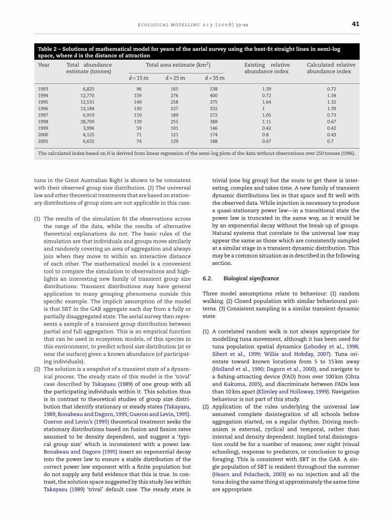
vey data. The three unknown quantities in the model are areaof aggregation (A), time over which aggregation occurs (t) anddistance of interaction (d) (Eq. (4)). Assuming tuna congregateusing sight over 5 h in the mornings, values of A (total area inkm2) were calculated for d (attractive distances) of 15, 25 and35 m (Table 2). This period of aggregation is consistent withanecdotal observations of fishers and by the very few stud-ies that have been made of whole schools of tuna via sidescan sonar at fish aggregating devices (FADs) (Schaefer andFuller, 2005)). The total area of the survey is about 184,000 km2,and the results suggest a total area of aggregation of about60–400 km2. The results would be consistent with the exis-tence of one or more cells of aggregation inside the overallarea of occurrence.

6. Discussion

6.1. Fundamental agreement with rules underlying

universal law

There are two new implications of this study: (1) the simu-lation model of the individual behaviour of southern bluefin

e c o l o g i c a l m o d e l l i n g 2 1 3 ( 2 0 0 8 ) 33–44 41

Table 2 – Solutions of mathematical model for years of the aerial survey using the best-fit straight lines in semi-logspace, where d is the distance of attraction

Year Total abundanceestimate (tonnes)

Total area estimate (km2) Existing relativeabundance index

Calculated relativeabundance index

d = 15 m d = 25 m d = 35 m

1993 6,825 96 165 238 1.39 0.721994 12,770 159 276 400 0.72 1.341995 12,531 149 258 375 1.64 1.321996 13,184 130 227 332 1 1.391997 6,919 110 189 272 1.05 0.731998 28,709 139 255 388 1.11 0.671999 3,996 59 101 146 0.42 0.422000 4,125 71 121 174 0.8 0.432005 6,632 74 129 188 0.67 0.7

he se

twla

(

(

foraging. This is consistent with SBT in the GAB. A sin-

The calculated index based on N is derived from linear regression of t

una in the Great Australian Bight is shown to be consistentith their observed group size distribution. (2) The universal

aw and other theoretical treatments that are based on station-ry distributions of group sizes are not applicable in this case.

1) The results of the simulation fit the observations acrossthe range of the data, while the results of alternativetheoretical explanations do not. The basic rules of thesimulation are that individuals and groups move similarlyand randomly covering an area of aggregation and alwaysjoin when they move to within an interactive distanceof each other. The mathematical model is a convenienttool to compare the simulation to observations and high-lights an interesting new family of transient group sizedistributions. Transient distributions may have generalapplication to many grouping phenomena outside thisspecific example. The implicit assumption of the modelis that SBT in the GAB aggregate each day from a fully orpartially disaggregated state. The aerial survey then repre-sents a sample of a transient group distribution betweenpartial and full aggregation. This is an empirical functionthat can be used in ecosystem models, of this species inthis environment, to predict school size distribution (at ornear the surface) given a known abundance (of participat-ing individuals).

2) The solution is a snapshot of a transient state of a dynam-ical process. The steady state of this model is the ‘trival’case described by Takayasu (1989) of one group with allthe participating individuals within it. This solution thusis in contrast to theoretical studies of group size distri-bution that identify stationary or steady states (Takayasu,1989; Bonabeau and Dagorn, 1995; Gueron and Levin, 1995).Gueron and Levin’s (1995) theoretical treatment seeks thestationary distributions based on fusion and fission ratesassumed to be density dependent, and suggest a ‘typi-cal group size’ which is inconsistent with a power law.Bonabeau and Dagorn (1995) insert an exponential decayinto the power law to ensure a stable distribution of the

correct power law exponent with a finite population butdo not supply any field evidence that this is true. In con-trast, the solution space suggested by this study lies withinTakayasu (1989) ‘trival’ default case. The steady state is

mi-log plots of the data without observations over 250 tonnes (1996).

trivial (one big group) but the route to get there is inter-esting, complex and takes time. A new family of transientdynamic distributions lies in that space and fit well withthe observed data. While injection is necessary to producea quasi-stationary power law—in a transitional state thepower law is truncated in the same way, as it would beby an exponential decay without the break-up of groups.Natural systems that correlate to the universal law mayappear the same as those which are consistently sampledat a similar stage in a transient dynamic distribution. Thismay be a common situation as is described in the followingsection.

6.2. Biological significance

Three model assumptions relate to behaviour: (1) randomwalking. (2) Closed population with similar behavioural pat-terns. (3) Consistent sampling in a similar transient dynamicstate.

(1) A correlated random walk is not always appropriate formodelling tuna movement, although it has been used fortuna population spatial dynamics (Lehodey et al., 1998;Sibert et al., 1999; Willis and Hobday, 2007). Tuna ori-entate toward known locations from 5 to 15 km away(Holland et al., 1990; Dagorn et al., 2000), and navigate toa fishing-attracting device (FAD) from over 100 km (Ohtaand Kakuma, 2005), and discriminate between FADs lessthan 10 km apart (Klimley and Holloway, 1999). Navigationbehaviour is not part of this study.

(2) Application of the rules underlying the universal lawassumed complete disintegration of all schools beforeaggregation started, on a regular rhythm. Driving mech-anism is external, cyclical and temporal, rather thaninternal and density dependent. Implied total disintegra-tion could be for a number of reasons; over night (visualschooling), response to predators, or conclusion to group

gle population of SBT is resident throughout the summer(Hearn and Polacheck, 2003) so no injection and all thetuna doing the same thing at approximately the same timeare appropriate.

l i n g

42 e c o l o g i c a l m o d e l

(3) Other natural group size distributions, without a −1.5exponent (Bonabeau et al., 1998), may now be explained astransient dynamical distributions before reaching steadystate. Aggregation may be halted by behaviour or envi-ronment, followed by repeated sampling. This questionsthe process of grouping as behaviour and whether it is adistinct process to other group activities. That is, do fish(1) form a group, and then (2), act as a group, as two dis-tinct behavioural modes? If true, we may often see the sizedistribution ‘frozen’ in a transient state. Behaviour modeswitch may be triggered externally and related to time,prey, predators or environment. Even when able to ran-domly sample across the range of aggregation states theexponential decay in group numbers means that we wouldmore often sample in similar semi-aggregated states. Forinstance consider the similarity between the group sizedistributions of the simulation after 1000 and 1400 stepsas opposed to after 200 and 600 steps (Fig. 4), the distri-bution approaches a similar state and remains relativelyconstant over time. In the subject case of this study, aerialobservations were always started after 12 noon and conse-quently they may always be a sample of a relatively maturestate of aggregation.

6.3. The use of theoretical models in ecology

Consistent with the use of theoretical models in ecology; thenew model can be extended to explore hypotheses beyondthe facts to help plan field work (Mangel and Clark, 1988;Schmitz, 2001; Odenbaugh, 2005). This relates to solutions tothe equations for areas of attraction (which relates to sen-sory capability) and total area of disaggregating (relates tobehaviour while not grouped). The results predict that theareas over which the schools form are less than the total areaof occurrence. This is true in the natural system in that schoolsform in similar locations each year, at the shelf edge andaround inshore reefs (Schahinger, 1987; Gunn and Young, 1996;Davis and Stanley, 2002). An alternative interpretation, usingdifferent model calibration, is that schools remain grouped,steadily growing for days or weeks, while moving across largerareas. This second explanation is inconsistent with recentfield observation (Willis and Hobday, 2007). Different interpre-tation may be appropriate for schools in the open ocean, wherealso constant injection may have biological significance andmeeting points may be transient, more diffuse, mobile and lessobvious than fixed bathymetric features. Observations fromfisheries data may also require different treatment as tunaare often attracted to boats and fishers exploit this behaviour,augmented with bait.

6.4. Using the models to extend earlier studies

The simulation model could be configured to replicate theresult of the Takayasu grid model. If new individuals were con-stantly injected, the model output of group size distributionapproximated a power law with exponent of −1.5. The grid

model is thus extended from dimensionless to two dimen-sions and this demonstrates the power law is persistent. Thiscontradicts Bonabeau and Dagorn (1995) who suggest that thepower law exponent is dependent on the space in which the

2 1 3 ( 2 0 0 8 ) 33–44

fish move being less than three dimensions (Bonabeau et al.,1998). This applies to spaces which are effectively closer to twodimensions—for instance if the fish aggregate in a particulardepth layer, or against a linear bathymetric feature (Bonabeauet al., 1999). Turbidity, ocean frontal systems, temperature,light and weather may all cause variation in the rate of forma-tion of groups, but the analysis here shows that, as long as theyaffect all group size interactions similarly, they will not alterthe −1.5 gradient of the power law section of the group sizedistribution. This may account for the persistence of this gra-dient in many different natural and simulated systems and itsconsequent lack of utility in deriving other interesting systemparameters.

6.5. Potential enhancements to improve realism

In order to check the sensitivity of the result to potentialincreases in realism, I investigated two enhancements to thebasic simulation: (1) to change the attractive distance depen-dent on size of group and (2) to change the tortuosity ofmovement dependent on size of group.

(1) A large school could be 20–50 m in lateral dimension,so the interactive distance may be twice or three timesthat of a single fish or small group. Furthermore, ‘rip-pling’ behaviour of tuna in large schools might causereflections to flash over wide areas underwater, furtherincreasing attractive area. Rippling is also hypothesised tobe about insolating warmth (Gunn et al., 1995). I testedthe sensitivity of the simulation to attractive distancesincreasing linearly proportional to group size, increasingthe attractive distances up to 10 times for the largestgroups. Extreme cases of changes to attractive distanceresulted in all groups forming more quickly. Increasedinteractive distance for large groups affects the numberof small groups as well as they both combine more often.For more moderate increases in attractive distance, up tothree times the value of the small groups for larger groups,the results were indistinguishable from the base case ofequal attractive distances.

(2) To test the second enhancement, I increased the tortuos-ity linearly in proportion to group size. The logic is that,without any bias in direction, a large school in realitymay not have the same freedom of movement as a sin-gle fish or small school. The situation has been explicitlyexplored using similar simulation models (Codling, 2007).I increased the tortuosity factor (TF) from 10% (whichequates to new angles selected from a random normaldistribution with standard deviation 36◦) to a maximumof 60% linearly proportional to group size. A TF of 60% pro-duces a path very close to an undirected random walk andsignificantly reduces the area of movement, with the pathcrossing back over itself very often. In the extreme case allgroups formed more slowly. In the more moderate cases(a max. TF of 30%) the results were indistinguishable fromthe default case.

Both enhancements had an indiscernible effect at modestlevels. They had similar, but opposite, effects at more extremelevels. No field data are available to parameterise either; there-

n g

ftac

A

ALBCsRaSMa

r

A

B

B

B

B

B

C

C

C

C

C

D

D

F

F

e c o l o g i c a l m o d e l l i

ore neither is included in the simulation. It is possible thathey are realistic effects in the field but that their resultantlteration of the group size distributions, in this case, is indis-ernible due to the quality of the field data we have.

cknowledgements

listair Hobday, Jessica Farley, Hiro-Sato Niwa, Yoshimi Takao,aurent Dagorn, Richard Coleman, Volker Grimm, Marinelleasson, Mark Bravington, Tom Polachek, Paige Eveson, andampbell Davies, all helped with the preparation of thistudy and reviewed and improved the manuscript. The SBTecruitment Monitoring Program made the aerial survey datavailable. The study was prompted by an original idea ofachiko Tsuji at the 17th workshop of the SBT Recruitmentonitoring Program 2005. I appreciate the assistance of two

nonymous reviewers in final preparation of the manuscript.

e f e r e n c e s

oki, I., 1982. A simulation study on the schooling mechanism infish. Bull. Jpn. Soc. Sci. Fish. 48, 1081–1088.

ak, P., 1997. How Nature Works. The Science of Self-organizedCriticality. Oxford University Press, Oxford.

asson, M., Bravington, M., Everson, P., Farley J., 2005. Preliminaryresults of aerial survey and commercial spotting data. In:Southern Bluefin Tuna Recruitment Monitoring WorkshopReport. RMWS/05/01. CSIRO Marine Laboratories, Hobart.

onabeau, E., Dagorn, L., 1995. Possible universality in the sizedistribution of fish schools. Phys. Rev. E 51, R5220–R5223.

onabeau, E., Dagorn, L., Freon, P., 1998. Space dimension andscaling in fish school-size distributions. J. Phys. A-Math. Gen.31, L731–L736.

onabeau, E., Dagorn, L., Freon, P., 1999. Scaling in animalgroup-size distributions. Proc. Natl. Acad. Sci. U.S.A. 96,4472–4477.

amacho, J., Sole, R.V., 2001. Scaling in ecological size spectra.Europhys. Lett. 55, 774–780.

amazine, S., Deneubourg, J.-L., Franks, N.R., Sneyd, J., Theraulaz,G., Bonabeau, E., 2003. Self-organisation in Biological Systems.Princeton University Press.

lark, C.W., Mangel, M., 1986. The evolutionary advantages ofgroup foraging. Theor. Popul. Biol. 30, 45–75.

odling, E.A., 2007. Group navigation and the ‘many wrongsprinciple’ in models of animal movement. Ecology 88,1864–1870.

owling A., Polacheck T., Miller C., 1996. Data analysis of theaerial surveys (1991–1996) for juvenile Southern bluefin tunain the Great Australian Bight. In: Southern bluefin tunarecruitment monitoring workshop report. RMWS/96/4. CSIROMarine Laboratories, Hobart, p 87.

agorn, L., Josse, E., Bach, P., Bertrand, A., 2000. Modeling tunabehaviour near floating objects: from individuals toaggregations. Aquat. Living Resour. 13, 203–211.

avis, T.L.O., Stanley, C.A., 2002. Vertical and horizontalmovements of southern bluefin tuna (Thunnus maccoyii) in theGreat Australian Bight observed with ultrasonic telemetry.Fish. B-NOAA 100, 448–465.

raenkel, G., Gunn, D., 1940. The Orientation of Animals. Dover

Publications Ltd., London.

ritz, H., Said, S., Weimerskirch, H., 2003. Scale-dependenthierarchical adjustments of movement patterns in along-range foraging seabird. Proc. Roy. Soc. Lond. B Bio. 270,1143–1148.

2 1 3 ( 2 0 0 8 ) 33–44 43

Fulton, E.A., Smith, A.D.M., Johnson, C.R., 2003. Effect ofcomplexity on marine ecosystem models. Mar. Ecol. Prog. Ser.253, 1–16.

Grimm, V., Berger, U., Bastiansen, F., Eliassen, S., Ginot, V., Giske,J., Goss-Custard, J., Grand, T., Heinz, S.K., Huse, G., Huth, A.,Jepsen, J.U., Jorgensen, C., Mooij, W.M., Muller, B., Pe’er, G.,Piou, C., Railsback, S.F., Robbins, A.M., Robbins, M.M.,Rossmanith, E., Ruger, N., Strand, E., Souissi, S., Stillman, R.A.,Vabo, R., Visser, U., DeAngelis, D.L., 2006. A standard protocolfor describing individual-based and agent-based models. Ecol.Model. 198, 115–126.

Gueron, S., Levin, S.A., 1995. The dynamics of group formation.Math. Biosci. 128, 243–264.

Gunn, J., Young, J., 1996. Environmental determinants of themovement and migration of juvenile southern bluefin tuna.In: Fish movement and Migration. Workshop proceeding.Australian Society for Fish Biology, Sydney.

Gunn, J., Davis, T., Polachek, T., Betlehem, A., Sherlock, M., 1995.The application of archival tags to study SBT migration,behaviour and physiology. In: Southern bluefin tunarecruitment monitoring workshop report. RMWS/95/8. CSIROMarine Laboratories, Hobart.

Hearn, W.S., Polacheck, T., 2003. Estimating long-termgrowth-rate changes of southern bluefin tuna (Thunnusmaccoyii) from two periods of tag-return data. Fish. B-NOAA101, 58–74.

Holland, K.N., Brill, R.W., Chang, R.K.C., 1990. Horizontal andvertical movements of yellowfin and bigeye tuna associatedwith fish aggregating devices. Fish. B-NOAA 88, 493–507.

Holling, C.S., 1959. Some characteristics of simple types ofpredation and parasitism. Can. Entomol. 91, 385–398.

Huth, A., Wissel, C., 1992. The simulation of the movement of fishschools. J. Theor. Biol. 156, 365–385.

Klimley, A.P., Holloway, C.F., 1999. School fidelity and homingsynchronicity of yellowfin tuna Thunnus albacares. Mar. Biol.133, 307–317.

Lehodey, P., Andre, J.M., Bertignac, M., Hampton, J., Stoens, A.,Menkes, C., Memery, L., Grima, N., 1998. Predicting skipjacktuna forage distributions in the equatorial Pacific using acoupled dynamical bio-geochemical model. Fish Oceanogr. 7,317–325.

Mandelbrot, B.B., 1967. How long is the coast of Britain. Science156, 636–638.

Mangel, M., Clark, C.W., 1988. Dynamic Modeling in BehavioralEcology. Princeton University Press, Princeton, NJ.

Manrubia, S.C., Zanette, D.H., Sole, R.V., 1999. Transientdynamics and scaling phenomena in urban growth.FRACTALS 7, 1–8.

Nams, V., 2006. Detecting orientated movement of animals.Anim. Behav. 72, 1197–1203.

Odenbaugh, J., 2005. Idealized, inaccurate but successful: apragmatic approach to evaluating models in theoreticalecology. Biol. Philos. 20, 231–255.

Ohta, I., Kakuma, S., 2005. Periodic behavior and residencetime of yellowfin and bigeye tuna associated with fishaggregating devices around Okinawa Islands, asidentified with automated listening stations. Mar. Biol. 146,581–594.

Partridge, B.L., 1982. The Structure and Function of Fish Schools.Scientific American, 114-183.

Petitgas, P., Reid, D., Carrera, P., Iglesias, M., Georgakarakos, S.,Liorzou, B., Masse, J., 2001. On the relation between schools,clusters of schools, and abundance in pelagic fish stocks. IcesJ. Mar. Sci. 58, 1150–1160.

Ruxton, G.D., Fraser, C., Broom, M., 2005. An evolutionarilystable joining policy for group foragers. Behav. Ecol. 16,856–864.

Schaefer, K.M., Fuller, D.W., 2005. Behavior of bigeye (Thunnusobesus) and skipjack (Katsuwonus pelamis) tunas within

l i n g

44 e c o l o g i c a l m o d e l

aggregations associated with floating objects in the equatorialeastern Pacific. Mar. Biol. 146, 781–792.

Schahinger, R.B., 1987. Structure of coastal upwelling eventsobserved off the southeast coast of South-Australia duringFebruary 1983–April 1984. Aust. J. Mar. Fresh Res. 38, 439–459.

Schmitz, O.J., 2001. From interesting details to dynamicalrelevance: toward more effective use of empirical insights intheory construction. OIKOS 94, 39–50.

Sibert, J.R., Hampton, J., Fournier, D.A., Bills, P.J., 1999. Anadvection-diffusion-reaction model for the estimation of fishmovement parameters from tagging data, with application to

skipjack tuna (Katsuwonus pelamis). Can. J. Fish Aquat. Sci. 56,925–938.

Sole, R.V., Manrubia, S.C., Benton, M., Kauffman, S., Bak, P., 1999.Criticality and scaling in evolutionary ecology. Trends Ecol.Evol. 14, 156–160.

2 1 3 ( 2 0 0 8 ) 33–44

Takayasu, H., 1989. Steady-state distribution of generalizedaggregation system with injection. Phys. Rev. Lett. 63,2563–2565.

Turchin, P., 1998. Quantitative Analysis of Movement. SinauerAssociates Inc., Sunderland, MA, USA.

Turcotte, D.L., Malamud, B.D., 2004. Landslides, forest fires, andearthquakes: examples of self-organized critical behavior.Physica A 340, 580–589.

Utsu, T., Ogata, Y., Matsuura, R.S., 1995. The centenary of theOmori formula for a decay law of aftershock activity. J. Phys.Earth 43, 1–33.

Warburton, K., Lazarus, J., 1991. Tendency distance models ofsocial cohesion in animal groups. J. Theor. Biol. 150, 473–488.

Willis, J., Hobday, A.J., 2007. Influence of upwelling on movementof southern bluefin tuna (Thunnus maccoyii) in the GreatAustralian Bight. Mar. Freshwater Res. 58, 699–708.