www.elsevier.com/locate/margeo

Marine Geology 215

Seismic inversion for acoustic impedance and porosity of

Cenozoic cool-water carbonates on the upper continental

slope of the Great Australian Bight

M. Huusea,*, D.A. Fearyb,1

a3DLab, School of Earth, Ocean and Planetary Sciences, Cardiff University, Wales, UKbAustralian Geological Survey Organization, Canberra, Australia

Received 30 September 2004; received in revised form 17 December 2004; accepted 21 December 2004

Abstract

Seismic inversion is used to estimate detailed seismic and rock properties, such as acoustic impedance and porosity, from

seismic data. Themethod is widely used and proven successful by the petroleum industry, but has hitherto not beenwidely adopted

for academic studies. This paper outlines a workflow and reports the application of model-based seismic inversion to a Cenozoic

cool-water carbonate succession on the upper continental slope of the Great Australian Bight that was cored during Ocean Drilling

Program Leg 182. Acoustic impedance data and the derived porosity distribution facilitate detailed studies of lithology,

compaction and fluid flow in the shallow subsurface (0–500m). A comparison of reflection and impedance data support the notion

that seismic reflection events arise from bed boundaries rather than from lateral changes in impedance, even where these are

significant. The uppermost continental slope of SWAustralia is swept by a strong (N0.5 m/s) geostrophic current, the Leeuwin

Current, and seismic profiles across the upper slope show geometrical similarities with contourite drifts. Cores taken through a

conspicuous mounded seismic facies at ODP Site 1131 suggest that bryozoan build-ups nucleated on top of contourite mounds on

the uppermost slope. Core recovery at three sites on a transect across the uppermost continental slope systematically decreased

with increasing acoustic impedance and depth of the drilled section regardless of age. Because of the enhanced interpretability

afforded by acoustic impedance and porosity data, and the possibility of predicting core recovery, the workflow outlined here

should be of use in a broad spectrum of continental margin studies.

D 2004 Elsevier B.V. All rights reserved.

Keywords: seismic inversion; acoustic impedance; carbonate; contourite; Great Australian Bight; ODP Leg 182

0025-3227/$ - see front matter D 2004 Elsevier B.V. All rights reserved.

doi:10.1016/j.margeo.2004.12.005

* Corresponding author.

E-mail address: m.huuse@earth.cf.ac.uk (M. Huuse).1 Present address: Board on Earth Sciences and Resources,

National Research Council, Washington, DC, USA.

1. Introduction

Seismic reflection profiles provide images of

relative subsurface variations of acoustic impedance,

(2005) 123–134

M. Huuse, D.A. Feary / Marine Geology 215 (2005) 123–134124

i.e., they show the distribution of interfaces between

layers with different acoustic properties. Acoustic

impedance is the product of rock density and

compressional (P-wave) velocity. It is thus a measure

of physical properties that are commonly measured in

boreholes, such as bulk density and sonic velocity, as

well as being qualitatively observed in core and

outcrop as the dhardnessT of the rock. Seismic

inversion is a method of deriving seismic parameters,

such as acoustic impedance, from reflection seismic

data constrained by borehole data (e.g., Sheriff and

Geldart, 1995; Veeken and Da Silva, 2004). This

information may be used to derive the detailed

porosity and lithology structure of the subsurface,

provided there is a link between porosity (or

lithology) and acoustic impedance (Anselmetti and

Eberli, 1997; Marion and Jizba, 1997).

Seismic inversion for acoustic impedance is widely

used for subsurface interpretation by the petroleum

industry, particularly in settings where a unique

relation between acoustic impedance and porosity

can be established (e.g., Marion and Jizba, 1997). A

suite of inversion methods has been developed in

response to the need for detailed subsurface mapping

of porosity and pore-fluid variations as part of the

petroleum industry’s hunt for increasingly subtle oil

and gas reservoirs (Maver and Rasmussen, 1995;

Buiting and Bacon, 1999; van Riel, 2000; Story et al.,

2000; Veeken and Da Silva, 2004). The increasing

number of oil discoveries that have been made using

inverted seismic data has confirmed that inversion is

indeed a powerful means for enhancing the interpret-

ability of seismic data (e.g., Buiting and Bacon, 1999;

Vejb&k and Kristensen, 2000). Apart from their use

for standard reservoir interpretation, rock property

data and their derivatives (such as porosity) are useful

for a range of other studies that include fluid flow and

continental slope stability (e.g., Dugan and Flemings,

2000; Bunz and Mienert, 2004). Consequently, there

has been a recent shift in emphasis from inversion

focused at petroleum reservoir levels to also include

the overburden to prospective intervals in the inver-

sion. Such studies have proven particularly useful for

inferring drilling hazards caused by shallow gas or

overpressured intervals (e.g., Dutta, 2002; Dai et al.,

2004; Salisbury et al., 2004). However, despite the

advantages of impedance data for shallow hazard

detection and for seismic facies and lithology inter-

pretation, inversion methods have so far not been

widely adopted for non-petroleum research, such as,

e.g., the majority of the ocean drilling (DSDP, ODP,

iODP) activities. This is despite the fact that boreholes

are tied to detailed site surveys and regional seismic

surveys using synthetic seismic and seismic modelling

as an integral part of both academic and industrial

drilling programs (e.g., Lorenzo and Hesselbo, 1996).

When well-to-seismic ties have been made, and a

wavelet has been extracted, the final step of inverting

the data is comparatively straightforward.

This paper presents the workflow and application

of model-driven seismic inversion to estimate the

acoustic impedance and porosity of Cenozoic cool-

water carbonates in the Great Australian Bight, using

seismic data collected during site surveys (Feary,

1997) as well as core and borehole log data acquired

during Ocean Drilling Program (ODP) Leg 182 (Feary

et al., 2000, 2004). After outlining the method for

deriving the acoustic impedance section and estimat-

ing porosity, we discuss the enhanced interpretability

afforded by the impedance data by looking at the

internal structure of carbonate mounds and discussing

the origin and significance of reflections within the

Pleistocene slope succession. The advantages for

interpretation and the relationship between core

recovery and acoustic impedance makes seismic

inversion a powerful tool that could be useful for

most integrated studies of borehole and seismic data.

2. Geological setting: the Great Australian Bight

The Great Australian Bight is a siliciclastic-

starved, passive continental margin bordering the

Southern Ocean. The uppermost continental slope

along SW Australia is swept by a strong geostrophic

current, the Leeuwin Current, and associated coun-

ter-flow and eddies, the intensities of which vary on

multiple time scales (Cresswell and Peterson, 1993;

Creswell and Griffin, 2004). The target of the ODP

Leg 182 drilling campaign was an improved under-

standing of the factors that controlled cool-water

carbonate deposition of Eocene to Quaternary

sequences on the continental shelf, slope and basin

(Feary and James, 1998; Feary et al., 2000, 2004).

The shelf edge to upper slope in the Great

Australian Bight consists of a spectacular succession

M. Huuse, D.A. Feary / Marine Geology 215 (2005) 123–134 125

of progradational clinoforms forming an approxi-

mately 500 m thick wedge of Pleistocene cool-water

carbonates (Fig. 1; Feary and James, 1998; Hine et

al., 1999; Feary et al., 2000, 2004; James et al.,

2000). Leg 182 Sites 1127, 1131 and 1129 form a

closely spaced dip transect across this uppermost

slope wedge (Fig. 1). The sediments forming the

slope wedge are packstones to wackestones contain-

ing a wide variety of skeletal grains produced on

the adjacent shelf (Hine et al., 1999; Feary et al.,

2000, 2004).

Apart from the unusually thick Pleistocene

succession, Leg 182 also cored uppermost Cenozoic

bryozoan mounds located at present-day water

depths of ~200–350 m (Fig. 1; Feary and James,

1995, 1998; Feary et al., 2000; James et al., 2000),

Fig. 1. Seismic line illustrating the progradational clinoforms and moun

beneath the Eucla Shelf and upper slope. Vertical scale is two-way travel ti

m on the slope to about 170 m on the shelf. The extent of the strong, eas

reference (cf. Cresswell and Peterson, 1993). ODP Leg 182 Sites 1129, 11

curve) and reflectivity (denoted R~white curve) logs. Interpreted seismic ho

indicated by arrows in the upper right corner of the inset, which also sho

sequence subdivision are according to Feary and James (1998) and Feary

and intersected abnormally high concentrations of

hydrogen sulfide and methane within the sediment

succession (Swart et al., 2000; Mitterer et al.,

2001).

3. Subsurface database

A grid of high-resolution, multichannel reflection

seismic profiles was used to choose drilling loca-

tions for the ODP Leg 182 drill sites (Feary and

James, 1998; Feary et al., 2000, 2004). The stacked

and time-migrated seismic data are zero phased,

sampled at 2 ms and have a dominant frequency of

about 100 Hz. This corresponds to a dominant

wavelength of 15–25 m at subsurface interval

ds that constitute the upper Cenozoic cool-water carbonate wedge

me (TWT). The water depth along the profile varies from about 750

tward flowing Leeuwin current at the uppermost slope is shown for

27 and 1131 are shown with acoustic impedance (denoted AI~black

rizons are shown as black lines. The location of the seismic profile is

ws the location of all Leg 182 boreholes. Seismic stratigraphy and

et al. (2000).

M. Huuse, D.A. Feary / Marine Geology 215 (2005) 123–134126

velocities between 1.5 and 2.5 km/s and is

equivalent to an approximate vertical seismic

resolution (one quarter of the dominant wavelength)

of about 5 m.

The drilled section mainly consists of Pleistocene

carbonates of varying grain size and lithification

(Feary et al., 2000, 2004). Composite logs of sonic

(P-wave) velocity and formation density were

compiled for each site, primarily using downhole

log data. The uppermost ~100 m of each hole could

not be logged with downhole instruments, so the

downhole data were supplemented with a range of

shipboard core measurements for this interval-along-

core sonic velocity measurements, Vp(z), and

gamma-ray attenuation porosity evaluation

(GRAPE) density. Site 1127 was not logged with

the downhole density tool, and consequently, ship-

board density measurements were used for the

entire density log at this site. Because the sediment

cores expanded as they were brought to the surface,

the laboratory-measured values of velocity and

density are slightly lower than expected from

extrapolation of the downhole measurements. This

is seen as a minor (~10%) shift in the absolute

acoustic impedance at ~100 m subsurface, and

shallower values thus represent minimum values of

acoustic impedance.

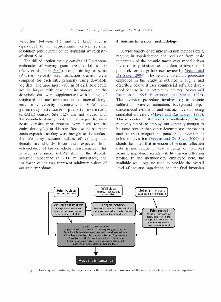
Fig. 2. Flow diagram illustrating the major steps in the model-driv

4. Seismic inversion—methodology

A wide variety of seismic inversion methods exist,

ranging in sophistication and precision from basic

integration of the seismic traces over model-driven

inversion of post-stack seismic data to inversion of

pre-stack seismic gathers (see review by Veeken and

Da Silva, 2004). The seismic inversion procedure

employed in this study is outlined in Fig. 2 and

described below; it uses commercial software devel-

oped for use in the petroleum industry (Maver and

Rasmussen, 1995; Rasmussen and Maver, 1996).

The inversion procedure involves log to seismic

calibration, wavelet estimation, background impe-

dance-model estimation and seismic inversion using

simulated annealing (Maver and Rasmussen, 1995).

This is a deterministic inversion methodology that is

relatively simple to employ, but generally thought to

be more precise than other deterministic approaches

such as trace integration, sparse-spike inversion or

coloured inversion (Veeken and Da Silva, 2004). It

should be noted that inversion of seismic reflection

data is non-unique in that a range of (relative)

acoustic impedance results will fit a given reflection

profile. In the methodology employed here, the

available well logs are used to provide the overall

level of acoustic impedance, and the final inversion

en inversion of the seismic data to yield acoustic impedance.

40000

-6000

Amplitude

0

2

4

6

8

10

12

Tim

e (s

ampl

es)

Fig. 3. The wavelet derived at Site 1129 and used in the inversion.

Very similar wavelets were derived at Sites 1127 and 1131,

indicating that one wavelet can be used to invert the entire seismic

profile.

0.2

0.4

0.6

1

1.2

1.4

TW

T(s

)

1.38e+06 Impedance (kg/m s2) 7.39e+06

0.2

0.4

0.6

1

1.2

1.4

TW

T(s

)

1.38e+06 Impedance (kg/m s2) 7.39e+06

Water column

Core-basedacousticimpedance

Log-basedacousticimpedance

Relative acousticimpedance variationsderived from seismic data

Borehole-derived acousticimpedance at ODP Site 1131

Low-frequency AI model

Inversion-derived AI

Fig. 4. Quality-control plot for the seismic inversion at Site 1131. A

denotes acoustic impedance. Note the good overall fit between the

measured and the inversion-derived acoustic impedance, except fo

the abrupt impedance increase at the seabed (~0.45 s TWT). Also

shown is the low-pass filtered impedance log used in the absolute

(dpriorT) impedance model.

M. Huuse, D.A. Feary / Marine Geology 215 (2005) 123–134 127

result is thus relatively well constrained compared to

inversion results derived without absolute impedance

information.

4.1. Log to seismic calibration

First, seismic and borehole data are imported to

the inversion project, and the borehole data are

converted to two-way travel time using check shot

and/or integrated velocities from the sonic logs. The

logs are re-sampled to the sample interval of the

seismic data (2 ms). The composite sonic and

density logs are multiplied to yield an acoustic

impedance log, which describes downhole variations

in impedance. The impedance log is used to derive

a log of zero-offset reflectivity, R, which is the

parameter that governs the (zero-offset) seismic

reflection response of the subsurface. The reflectiv-

ity between two samples is defined as R=(AI2�AI1)

/(AI2+AI1), where AI2 is the acoustic impedance of

the lower sample and AI1 is the acoustic impedance

of the upper sample. The depth to time conversion

using check shots and/or sonic information yields a

rough calibration of seismic and borehole data.

After wavelet estimation (see below), the calibration

experiment is repeated using synthetic seismic data

to recalibrate the logs to the seismic data. After

readjustments of the depth to time calibration, a

new wavelet is estimated. This iterative loop is

continued until no further improvement is observed.

4.2. Wavelet estimation

Once the initial calibration is performed, a

wavelet is defined by deriving the convolution

operator between the reflectivity log and the

I

r

M. Huuse, D.A. Feary / Marine Geology 215 (2005) 123–134128

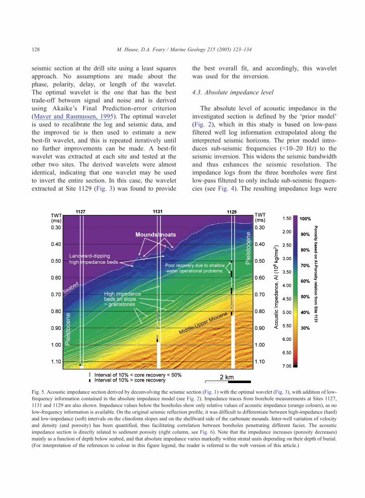
seismic section at the drill site using a least squares

approach. No assumptions are made about the

phase, polarity, delay, or length of the wavelet.

The optimal wavelet is the one that has the best

trade-off between signal and noise and is derived

using Akaike’s Final Prediction-error criterion

(Maver and Rasmussen, 1995). The optimal wavelet

is used to recalibrate the log and seismic data, and

the improved tie is then used to estimate a new

best-fit wavelet, and this is repeated iteratively until

no further improvements can be made. A best-fit

wavelet was extracted at each site and tested at the

other two sites. The derived wavelets were almost

identical, indicating that one wavelet may be used

to invert the entire section. In this case, the wavelet

extracted at Site 1129 (Fig. 3) was found to provide

Fig. 5. Acoustic impedance section derived by deconvolving the seismic se

frequency information contained in the absolute impedance model (see Fi

1131 and 1129 are also shown. Impedance values below the boreholes sho

low-frequency information is available. On the original seismic reflection p

and low-impedance (soft) intervals on the clinoform slopes and on the she

and density (and porosity) has been quantified, thus facilitating correla

impedance section is directly related to sediment porosity (right column,

mainly as a function of depth below seabed, and that absolute impedance v

(For interpretation of the references to colour in this figure legend, the re

the best overall fit, and accordingly, this wavelet

was used for the inversion.

4.3. Absolute impedance level

The absolute level of acoustic impedance in the

investigated section is defined by the dprior modelT(Fig. 2), which in this study is based on low-pass

filtered well log information extrapolated along the

interpreted seismic horizons. The prior model intro-

duces sub-seismic frequencies (b10–20 Hz) to the

seismic inversion. This widens the seismic bandwidth

and thus enhances the seismic resolution. The

impedance logs from the three boreholes were first

low-pass filtered to only include sub-seismic frequen-

cies (see Fig. 4). The resulting impedance logs were

ction (Fig. 1) with the optimal wavelet (Fig. 3), with addition of low-

g. 2). Impedance traces from borehole measurements at Sites 1127,

w only relative values of acoustic impedance (orange colours), as no

rofile, it was difficult to differentiate between high-impedance (hard)

lfward side of the carbonate mounds. Inter-well variation of velocity

tion between boreholes penetrating different facies. The acoustic

see Fig. 6). Note that the impedance increases (porosity decreases)

aries markedly within stratal units depending on their depth of burial.

ader is referred to the web version of this article.)

M. Huuse, D.A. Feary / Marine Geology 215 (2005) 123–134 129

then extrapolated along interpreted seismic horizons

to yield the absolute level of acoustic impedance

along the seismic profile. Constant values of absolute

impedance were assigned to the water column and to

the section below the drilled interval from which only

relative impedance values were derived (Fig. 5).

4.4. Seismic inversion

The seismic inversion uses the original seismic

data, the optimal wavelet and the background

impedance model (Fig. 2). To fully exploit the

information contained in the seismic data, the high-

frequency information from the boreholes is not used

in the inversion. The seismic inversion scheme used is

a globally optimized nonlinear method based on a

revised version of the simulated annealing algorithm

(Maver and Rasmussen, 1995; Rasmussen and Maver,

1996). The inversion is implemented by defining five

Acoustic imped

3*106 3.5*106 4*106 4.5*106

80

70

60

50

40

30

20

10

Por

osity

(%

)

Fig. 6. Relation between porosity and acoustic impedance at Site 1131. T

density and porosity logs) with a total of 2803 data points. The data show

caused by poor borehole conditions and resulting spurious data points. M

lines. The best-fit linear regression has a correlation factor of only 0.71 (R2

which is defined as 100% porosity and acoustic impedance of 1.5�106

relation was defined (green line) to enable impedance to porosity conver

colour in this figure legend, the reader is referred to the web version of th

parameters—signal/noise ratio and lateral continuity

of the seismic data, vertical variation in acoustic

impedance, prior model confidence, and the threshold

for layer interfaces (Fig. 2). The main result generated

by the seismic inversion is an acoustic impedance

section (Fig. 5), together with a variety of quality

control plots and other attributes (see Maver and

Rasmussen, 1995; Rasmussen and Maver, 1996).

4.5. Relation between acoustic impedance and porosity

A relation between subsurface acoustic impedance

and porosity can be established based on the Site 1131

downhole log measurements (Fig. 6). Because of non-

optimal hole conditions and resulting spurious down-

hole log measurements, there is a large scatter

superimposed on the natural variability of the acoustic

impedance–porosity relation. For simplicity, we

assume that the porosity to acoustic impedance

ance (kg*s/m2)

5*106 6*1065.5*106 6.5*106

he plot was constructed using unedited downhole log data (sonic,

a porosity–impedance relationship with a large scatter that is in part

aximum and minimum porosity envelopes are indicated with blue

~0.5). This best-fit linear regression does not pass through the origin,

kg/ms2 (corresponding to seawater). Therefore, a slightly modified

sion from the seabed down. (For interpretation of the references to

is article.)

M. Huuse, D.A. Feary / Marine Geology 215 (2005) 123–134130

relationship for the studied section can be described

by a single linear regression. Simple curve fits using

exponential, logarithmic, or power functions did not

yield improved correlations compared with the linear

fit. The best-fit linear regression does not yield a

realistic value for 100% porosity (seawater), and

hence, a slightly modified relation is used to convert

acoustic impedance to porosity: U=125�17AI, where

U is the porosity (%), and AI is the acoustic

impedance (106 kg/ms2). This relation is linear and

valid for porosity values z30% (the green line in Fig.

6). The acoustic impedance to porosity relation can be

used to convert the acoustic impedance section to a

porosity section (Fig. 5), which may be used to infer

lithology distribution, compaction state and fluid-flow

properties for the shallow subsurface. It is important

to note the large scatter (non-uniqueness) of the

porosity to acoustic impedance relationship (Fig. 6).

This means that for any single acoustic impedance

value, there is a wide range of possible porosity

values, e.g., from about 40% to 70% for an acoustic

impedance of 4.5�106 kg s m�2. Consequently, the

porosity conversion should only be considered a first

approximation, and a more refined relationship could

be established by estimating the relationship for

subsets of the data, e.g., based on mineralogy,

cementation, or texture (cf. Anselmetti and Eberli,

1997; Marion and Jizba, 1997).

5. Results and discussion

The main result of the seismic inversion study is a

profile showing the absolute variations in acoustic

impedance and porosity along a depositional dip

transect through Sites 1127, 1129 and 1131 (Fig. 5).

There is a very good fit between the acoustic

impedance values derived from the boreholes at each

drill site and the seismic inversion result. This was

expected from the wavelet extraction results for each

site, which indicated low variability in the seismic

source signature. Importantly, only the absolute level

of the acoustic impedance was included in the

inversion, i.e., no detailed well-log data were used,

and the fine-scale impedance variation is entirely due

to variations in the seismic reflection intensity.

The porosity distribution derived from the acoustic

impedance section (Fig. 5) and the impedance–

porosity relation (Fig. 6) are useful for a quantitative

determination of the lateral and vertical variations in

lithology and bed thickness between boreholes and

the porosity structure, and thus compaction state, of

the shallow subsurface. The latter may have implica-

tions for understanding the seabed stability and fluid-

flow behaviour of the investigated section, which in

turn contributes to understanding the conditions

leading to the unusual pore-fluid chemistry encoun-

tered in this part of the Great Australian Bight (Swart

et al., 2000; Mitterer et al., 2001). The following

sections describe a number of interesting observations

that were not readily apparent on the seismic

reflection profile (Fig. 1), but which can be made

using the acoustic impedance/porosity section (Fig.

5).

5.1. Acoustic impedance variation and seismic

reflections

The first thing to note about the inversion result is

that the absolute values of acoustic impedance and

porosity vary markedly within the individual seismic

sequences defined by Feary and James (1998) (e.g.,

from N45% to b30% porosity within the lowermost

Pleistocene sequence). This variation exceeds that seen

across stratal boundaries, and yet no seismic reflec-

tions arise from these lateral variations. This supports

the long-standing notion that seismic reflections

mainly follow stratal boundaries rather than lateral

facies variations (Vail et al., 1977). In this case, the

reason for the large lateral variation seems to be that

acoustic impedance and porosity are strongly depend-

ent on depth of burial (Fig. 5). Despite the large

magnitude of the variation within a given depositional

unit, lateral transitions are not observed in the seismic

reflection profile, which seems mainly to represent the

vertical impedance variations (compare Figs. 1 and 5).

It should be noted, however, that subtle variations in

horizon amplitude often seen in 3D seismic amplitude

maps may be able to pick up lateral facies changes not

readily observed with 2D seismic data.

High-amplitude reflection events occur on the

updip side of the seabed mounds and on the steeply,

seaward-dipping parts of the large clinoforms making

up the majority of the Pleistocene slope wedge (Fig.

1). The inversion result reveals that high-amplitude

reflections in the lower part of the succession around

M. Huuse, D.A. Feary / Marine Geology 215 (2005) 123–134 131

Site 1131 are due to high-impedance (hard) layers on

the clinoform foresets. These correspond to increased

abundances of grainstones and, to a lesser extent, to

increased abundance of more lithified intervals (Fig.

5; Feary et al., 2000). The correlation of high

impedance with grainstone intervals can be explained

by the greater velocity of grainstones compared to

more fine-grained carbonate mudstones in slope

environments, which may in turn be due to either a

greater stiffness or a greater diagenetic potential of

more permeable grainstones compared with more

muddy carbonates (Anselmetti and Eberli, 1997).

Whereas dbrightT reflections on seismic reflection

images highlight the presence of anomalous litholog-

ical units, the impedance data can be used to quantify

the lateral variations in thickness and/or facies of such

units, and thus can help to decipher the detailed

sedimentary facies distributions along the transect

away from areas of direct lithological control in wells,

as well as in those parts of the succession with poor

core recovery.

5.2. Geometry and origin of the upper slope succession

Seismic profiles across the Pleistocene upper slope

succession in the Great Australian Bight (Fig. 1) show

a 500-m-thick prograding wedge containing shelfward

accreting mound structures on the uppermost slope

and at the shelf break (Fig. 1; James et al., 2004). This

overall geometry is reminiscent of contourite drifts

seen along many continental margins (Faugeres et al.,

1999; Stow et al., 2002). Contourite drifts often

display upslope migration of more or less mounded

deposits that terminate upslope at erosional moats

(e.g., Faugeres et al., 1999). If the upper slope

succession seen in Figs. 1 and 5 were to be interpreted

geometrically in terms of contourite drift deposits, the

overall progradational slope wedge could be termed a

dslope plastered driftT (sensu Faugeres et al., 1999),

and the seabed and buried mounds could be termed

dmoat-related driftsT (sensu Faugeres et al., 1999) or

dmulti-crested driftT (sensu Howe et al., 2002),

depending on whether the moats are due to erosional

or depositional thinning. Given the relatively shallow

water depth of the upper slope and shelf break in the

Great Australian Bight (Fig. 1: ~750–150 m), the

upper slope succession would qualify as a dshallowwaterT contourite drift (sensu Stow et al., 2002).

Analysis of Leg 182 cores suggest that the

dominant provenance for the Pleistocene slope wedge

is the 200-km-wide Eucla shelf located immediately

to the north of the studied transect (Feary et al., 2000;

James et al., 2000, 2004). Mapping the geometry of

the moat-related mounds and mound complexes

shows that individual mounds may be up to 65 m

high and extend laterally for up to 10 km along strike

and up to 700 m perpendicular to the slope (Feary and

James, 1998; James et al., 2000). Seismic imagery of

the sequence of mounds cored at Site 1131 shows that

the locus of carbonate mound growth migrated

upslope towards the shelf (Fig. 1). The inversion

result shows that shelfward migrating high-amplitude

reflection events are due to high-impedance layers

(Fig. 5). These high-impedance layers could indicate

that fine-grained sediment may have been winnowed

from the upslope margin of the mounds, to leave a

coarser lag deposit. The mound that was cored at Site

1131 contained some 20–25 m of floatstone/rudstone

beds with well-preserved bryozoans, interpreted as a

bryozoan reef mounds preserved in situ (James et al.,

2000, 2004). However, the lower part of the core

taken in the mounded seismic facies consists of

bioclastic packstone, which is largely allochthonous

(Feary et al., 2000: chapter 9, Site 1131, p. 30). This

indicates that only the upper one-third of the mounded

seismic facies cored at Site 1131 represents bryozoan

mounds, and that the lower part achieved its mounded

appearance due to some other cause, prior to the

growth of the bryozoans.

The uppermost continental slope of SWAustralia is

swept by a strong geostrophic current, the Leeuwin

Current, which flows east along the uppermost

continental slope south of SW Australia at speeds in

excess of 0.5 m/s (Cresswell and Peterson, 1993;

James et al., 2000, 2004; Creswell and Griffin, 2004).

The eastward current is associated with a westward-

directed counterflow that may exceed 0.2 m/s located

downdip from the Leeuwin Current (Cresswell and

Peterson, 1993). The east–west flow patterns are

frequently distorted due to large-scale eddies (Cres-

well and Griffin, 2004), and any current influence on

sedimentation is thus expected to be highly complex.

Current velocities measured range up to 1.5 m/s with

0.5 m/s being common (Creswell and Griffin, 2004),

and this is strong enough to winnow relatively coarse

sediments and form scours in muddy sediments, and

M. Huuse, D.A. Feary / Marine Geology 215 (2005) 123–134132

certainly enough to shape the geometry of muddy

sediment drifts (Masson et al., 2004: their table 1 and

references therein).

It is thus conceivable that the overall geometry of

the Pleistocene upper slope succession in the Great

Australian Bight resulted from a combination of

abundant supply of carbonate muds and clasts derived

from the Eucla Shelf, and current-controlled redis-

tribution of these sediments on the uppermost slope

where the Leeuwin Current and related current

systems resulted in drift-like stratal geometries. In

this setting, conditions were intermittently favourable

for bryozoan organisms, which may locally have

formed reef mounds, perhaps preferentially nucleating

on the crests of pre-existing, current-controlled

mounds.

5.3. Hydrogen sulphide hydrates in the upper con-

tinental slope of the Great Australian Bight?

Unusually high concentrations of hydrogen sul-

phide and methane were encountered at Sites 1127,

1131 and 1129 (Feary et al., 2000). Swart et al. (2000)

speculated that the high concentrations of hydrogen

sulphide and methane might be due to the presence of

disseminated hydrogen sulphide and methane

hydrates. Gas hydrate-bearing sediments are usually

characterized by relatively high interval velocities due

to the solidity of the hydrate relative to pore water.

Because hydrates are generally associated with the

presence of free gas in the underlying section, their

presence usually causes a large decrease in acoustic

impedance at the hydrate base and a large impedance

increase at the gas–water interface below. The

hydrate–gas interface thus often gives rise to a bright

reflection event known as a bottom simulating

reflection (BSR), and the underlying gas interval

may be seen as a zone of anomalously low velocity

or low impedance (e.g., Bunz and Mienert, 2004; Dai

et al., 2004). However, no BSR is observed on the

high-quality reflection seismic data available (Fig. 1)

and no velocity inversion has been observed in the

wells or in the inversion data (Fig. 5). This supports the

previous suggestions by Swart et al. (2000) that any

hydrate, if present, would be highly disseminated and

that any free gas phase would be distributed with

sufficiently low gradients to not cause any seismic

anomalies.

5.4. Acoustic impedance and core recovery

Vertical zones of poor core recovery have been

plotted next to the borehole locations in Fig. 5. These

zones have been subdivided into poor (10–50%) and

very poor (b10%) recovery intervals indicated by

grey and black colour, respectively. The general trend

is one of decreased core recovery with increased

depth and increased lithification, especially where

discrete hard beds occur. Poor recovery at intermedi-

ate depths are most likely due to the use of the

extended core barrel (XCB) coring technique that was

generally employed for coring the intermediate parts

of the section (c. 200–500 m subsea) of Leg 182. This

technique, in combination with sea swells, will lead to

a dhammeringT effect on any lithified horizons, which

may lead to the liquefaction and thus poor recovery

potential of intervening softer intervals. In the case of

Sites 1129 and 1131, extreme lithification was

associated with the appearance of abundant thin

(few centimeters thick) chert layers in lower parts of

the section (Miocene), which made recovery of the

intervening, relatively soft carbonates impossible. At

Site 1129, some shallow intervals of poor core

recovery, not anticipated based from the impedance

data, were caused by shallow water operational

difficulties caused by a combination of long wave-

length sea swells and poor weather conditions (Feary

et al., 2000). Apart from the shallow poor recovery

intervals unrelated to the geology at Site 1129, there

is a clear tendency for recovery to be poor when

porosity decreases below about 40% (yellow-orange

colours in Fig. 5). This correlation seems sufficiently

strong that acoustic impedance data may be used to

predict broad trends in core recovery away from

points of borehole control. If this is relation is a

general one, it might be possible to use seismic

inversion as a cost-effective tool to optimize the

drilling strategy and recovery prediction of future

drilling campaigns, especially where borehole data

are available to calibrate the background impedance

model.

6. Conclusions

Seismic inversion for acoustic impedance is a well-

established tool in the petroleum industry where it has

M. Huuse, D.A. Feary / Marine Geology 215 (2005) 123–134 133

become a widely used method for optimizing the

quantitative analysis of seismic data to yield lithology

and porosity and permeability structure of the moder-

ately deep (~1–5 km) subsurface. Recently, the focus

has been widened to also include the shallow subsur-

face as this may be of interest to hazards studies and to

detailed studies of geological processes and products.

This study provides the first dacademicT application of

model-based seismic inversion using simulated anneal-

ing and demonstrates the enhanced interpretability of

acoustic impedance data as applied to the upper

continental slope of the Great Australian Bight.

Acoustic inversion shows that seismic reflections

in the upper slope succession originate from bed

boundaries rather than from lateral variations in

acoustic impedance, even if such impedance varia-

tions are of larger magnitude than those observed

across the individual bed boundaries. High amplitude

reflections visible on the seismic reflection section

mainly originate from high impedance (low porosity)

intervals within a relatively low impedance (high

porosity) slope wedge and in near-seabed mounds.

The overall geometry of the upper slope succession

in the Great Australian Bight, as seen in the studied

transect, displays many similarities with shallow-water

contourite drifts, including plastered slope drifts and

moat-related or multi-crested drifts. The study area is

presently dominated by a strong (N0.5 m/s) eastward

flowing geostrophic current, the Leeuwin Current, with

its associated counterflow and large-scale eddies,

which provide a complex current regime likely to

affect the deposition of both fine and coarse sediments

on the outer shelf and upper slope. Core data show that

only the upper one-third of the conspicuous mounded

seismic facies calibrated at Site 1131 contains in situ

bryozoans, whilst the lower two-thirds are comprised

of allochthonous muds. This could suggest that the

mounded facies represent contourite mounds capped

by bryozoan colonies.

No indications of gas hydrate or free gas were

found in the well logs or seismic data, and in parallel

with previous studies, it is suggested that any hydrate

present is disseminated and that the amount of free gas

in the upper 500 m of the slope wedge is minimal. A

rough correlation between zones of poor core recov-

ery and intervals of high impedance could suggest that

impedance data may be used to predict coring

performance away from already drilled sites.

Since acoustic impedance inversion for porosity

prediction may be undertaken wherever good quality

seismic and borehole data are available, the method

outlined here should be useful for most studies

dealing with sedimentary facies analysis, compaction

and fluid flow in the shallow subsurface.

Acknowledgements

The seismic inversion study was carried out during

a research stay by MH at the Borehole Research

Group of Lamont-Doherty Earth Observatory of

Columbia University, New York. The hospitality and

assistance by the people there is greatly appreciated.

MH acknowledges the support by Inge Lehmann’s

Legat af 1983 and DONGs Jubil&umslegat. adegaardA/S kindly supplied the seismic inversion software

(ISIS2D) used in the study and provided guidance for

its installation and use. Joe Cartwright and Richard

Davies provided helpful reviews of an earlier version

of the manuscript. The journal referees and editor

David Piper provided many valuable insights that

helped shape the final version of this article.

References

Anselmetti, F.S., Eberli, G.P., 1997. Sonic velocity in carbonate

sediments and rocks. In: Palaz, I., Marfurt, K.J. (Eds.),

Carbonate seismology, SEG Geophysical Developments Series,

vol. 6, pp. 53–74.

Buiting, J.J.M., Bacon, M., 1999. Seismic inversion as a vehicle for

integration of geophysical, geological and petrophysical infor-

mation for reservoir characterization: some North Sea examples.

In: Fleet, A.J., Boldy, S.A.R. (Eds.), Petroleum Geology of

Northwest Europe: Proceedings of the 5th Conference. Geo-

logical Society, London, pp. 1271–1280.

Bqnz, S., Mienert, J., 2004. Acoustic imaging of gas hydrate and

free gas at the Storegga Slide. J. Geophys. Res. 109 (B4), 4102.

Creswell, G.R., Griffin, D.A., 2004. The Leeuwin Current, eddies

and sub-Antarctic waters off south-western Australia. Mar.

Freshw. Res. 55 (3), 267–276.

Cresswell, G.R., Peterson, J.L., 1993. The Leeuwin Current south of

Western Australia. Aust. J. Mar. Freshw. Res. 44, 285–303.

Dai, J., Xu, H., Snyder, F., Dutta, N., 2004. Detection and

estimation of gas hydrates using rock physics and seismic

inversion: examples from the northern deepwater Gulf of

Mexico. Lead. Edge 23, 60–66.

Dugan, B., Flemings, P.B., 2000. Overpressure and fluid flow in the

New Jersey continental slope: implications for slope failure and

cold seeps. Science 289, 288–291.

M. Huuse, D.A. Feary / Marine Geology 215 (2005) 123–134134

Dutta, N.C., 2002. Geopressure prediction using seismic data:

current status and the road ahead. Geophysics 67, 2012–2041.

Faugeres, J.-C., Stow, D.A.V., Imbert, P., Viana, A., 1999. Seismic

features diagnostic of contourite drifts. Mar. Geol. 162, 1–38.

Feary, D.A. 1997. Cenozoic cool-water carbonates of the Great

Australian Bight: ODP Pollution Prevention and Safety Panel,

Leg 182 Safety Package. Australian Geological Survey Organ-

isation, Record 1997/28, 208 pp.

Feary, D.A., James, N.P., 1995. Cenozoic biogenic mounds and

buried Miocene (?) barrier reef on a predominately cool-water

carbonate continental margin—Eucla Basin, western Great

Australian Bight. Geology 23, 427–431.

Feary, D.A., James, N.P., 1998. Seismic stratigraphy and geological

evolution of the Cenozoic, cool-water Eucla Platform, Great

Australia Bight. AAPG Bull. 82, 792–816.

Feary, D.A., Hine, A.C., Leg 182 Shipboard Party, 2000. Proc. ODP,

Init. Repts., vol. 182. Texas A&M University, College Station,

TX. (CD-ROM, available from: Ocean Drilling Program).

Feary, D.A., Hine, A.C., James, N.P., Malone, M.J., 2004. Leg

182 Synthesis: exposed secrets of the Great Australian Bight.

In: Hine, A.C., Feary, D.A., Malone, M.J. (Eds.), Proc. ODP,

Sci. Results, vol. 182. Ocean Drilling Program, College Station,

TX, pp. 1–30.

Hine, A.C., Feary, D.A., Malone, M.J., Leg 182 Shipboard Party,

1999. Research in Great Australian Bight yields exciting early

results. EOS Trans. AGU 80, 521–526.

Howe, J.A., Stoker, M.S., Stow, D.A.V., Akhurst, M.C., 2002.

Sediment drifts and contourite sedimentation in the northeast-

ern Rockall Trough and Faroe-Shetland Channel, North

Atlantic Ocean. In: Stow, D.A.V., Pudsey, C.J., Howe, J.A.,

Faugeres, J.-C., Viana, A.R. (Eds.), Deep-water contourite

systems: modern drifts and ancient series, seismic and sedi-

mentary characteristics, Geological Society, London, Memoirs,

vol. 22, pp. 65–72.

James, N.P., Feary, D.A., Surlyk, F., Simo, T.J.A., Betzler, C.,

Holburn, A.E., Li, Q., Matsuda, H., Machiyama, H., Brooks,

G.R., Andres, M.S., Malone M.J., ODP Leg 182 Scientific

Party, 2000. Quaternary bryozoan reef mounds in cool-water,

upper slope environments: great Australian Bight. Geology 28,

647–650.

James, N.P., Feary, D.A., Betzler, C., Bone, Y., Holburn, A.E., Li,

Q., Machiyama, H., Simo, T.J.A., Surlyk, F., 2004. Origin of

late Pleistocene bryozoan reef mounds; Great Australian Bight.

J. Sediment. Res. 74 (1), 20–48.

Lorenzo, J.M., Hesselbo, S.P., 1996. Seismic-to-well correlation

of seismic unconformities at Leg 150 continental slope sites.

In: Mountain, G.S., Miller, K.G., Blum, P., Poag, C.W.,

Twichell, D.C. (Eds.), Proceedings of the Ocean Drilling

Program, Sci. Res., vol. 150. Ocean Drilling Program, College

Station, Texas, pp. 293–307.

Marion, D., Jizba, D., 1997. Acoustic properties in carbonate

rocks: use in quantitative interpretation of sonic and seismic

measurements. In: Palaz, I., Marfurt, K.J. (Eds.), Carbonate

seismology, SEG Geophysical Developments Series, vol. 6,

pp. 75–93.

Masson, D.G., Wynn, R.B., Bett, B.J., 2004. Sedimentary environ-

ment of the Faroe-Shetland Bank Channels, north-east Atlantic,

and the use of bedforms as indicators of bottom current velocity

in the deep ocean. Sedimentology 51, 1207–1241.

Maver, K.G., Rasmussen, K.B., 1995. Seismic inversion for

reservoir delineation and description. Soc. Pet. Eng. Paper

SPE29798, 267–275.

Mitterer, R.M., Malone, M.J., Goodfriend, G.A., Swart, P.K.,

Wortmann, U.G., Logan, G.A., Feary, D.A., Hine, A.C., 2001.

Co-generation of hydrogen sulfide and methane in marine

carbonate sediments. Geophys. Res. Lett. 28, 3931–3934.

Rasmussen, K.B., Maver, K.G., 1996. Direct inversion for

porosity of post stack seismic data. Soc. Pet. Eng.

SPE35509, 235–246.

Salisbury, R. Hamilton, I., Ayers, S. 2004. Dangerous shallow gas

and valuable oil and gas fields—A whole section view of

hydrocarbon reservoirs, paper presented at Seabed and Shallow

Section Marine Geoscience Conference, Geol. Soc., London,

24–26 February.

Sheriff, R.E., Geldart, L.P., 1995. Exploration seismology, 2nd ed.

Cambridge Univ. Press, Cambridge, USA.

Story, C., Peng, P., Lin, J.D., 2000. Liuhiua 11-1 field, South China

Sea: a shallow carbonate reservoir developed using ultrahigh-

resolution 3-D seismic, inversion, and attribute-based reservoir

modelling. Lead. Edge 19, 834–844.

Stow, D.A.V., Faugeres, J.-C., Howe, J.A., Pudsey, C.J., Viana,

A.R., 2002. Bottom currents, contourites and deep-sea sediment

drifts: current state of the art. In: Stow, D.A.V., Pudsey, C.J.,

Howe, J.A., Faugeres, J.-C., Viana, A.R. (Eds.), Deep-water

contourite systems: modern drifts and ancient series, seismic and

sedimentary characteristics, Geological Society, London, Mem-

oir, vol. 22, pp. 7–20.

Swart, P.K., Wortman, U., Mitterer, R., Smart, P.L., Feary, D.A.,

Hine, A.C., 2000. Hydrogen sulfide-rich hydrates and saline

fluids in the continental margin of South Australia. Geology 28,

1039–1042.

Vail, P.R., Todd, R.G., Sangree, J.B., 1977. Seismic stratigraphy and

global changes of sea level: Part 5. Chronostratigraphic

significance of seismic reflections. In: Payton, C.E. (Ed.),

Seismic stratigraphy—applications to hydrocarbon exploration,

AAPG Memoir, vol. 26, pp. 99–116.

van Riel, P., 2000. The past, present, and future of quantitative

reservoir characterization. Lead. Edge 19, 878–881.

Veeken, P.C.H., Da Silva, M., 2004. Seismic inversion methods and

some of their constraints. First Break 22, 47–70.

Vejb&k, O.V., Kristensen, L., 2000. Downflank hydrocarbon

potential identified using seismic inversion and geostatistics:

upper Maastrichtian reservoir unit, Dan Field, Danish Central

Graben. Pet. Geosci. 6, 1–13.