Quaternary Research 81 (2014) 274–283

Contents lists available at ScienceDirect

Quaternary Research

j ourna l homepage: www.e lsev ie r .com/ locate /yqres

A continuous multi-millennial record of surficial bivalve mollusk shellsfrom the São Paulo Bight, Brazilian shelf

Troy A. Dexter a,⁎, Darrell S. Kaufman b, Richard A. Krause Jr. c, Susan L. Barbour Wood d, Marcello G. Simões e,John Warren Huntley f, Yurena Yanes g, Christopher S. Romanek h, Michał Kowalewski a

a Florida Museum of Natural History, University of Florida, Gainesville, FL 32611, USAb School of Earth Sciences & Environmental Sustainability, Northern Arizona University, Flagstaff, AZ 86011, USAc Geosciences Institute, Johannes Gutenberg University, Johann-Joachim-Becher-Weg 21, Mainz 55128, Germanyd Rubicon Geological Consultants, 1690 Sharkey Rd., Morehead, KY 40351, USAe Instituto de Biociências, Universidade Estadual Paulista, Distrito de Rubião Junior, CP. 510, 18618-970 Botucatu, Brazilf Department of Geological Sciences, University of Missouri, Columbia, MO 65211, USAg Department of Geology, University of Cincinnati, Cincinnati, OH 45221, USAh Department of Earth and Environmental Sciences, University of Kentucky, Lexington, KY 40506, USA

⁎ Corresponding author at: Florida Museum of Natura1659 Museum Rd., P.O. Box 117800, Gainesville, FL 32611

E-mail address: tdexter@flmnh.ufl.edu (T.A. Dexter).

0033-5894/$ – see front matter © 2013 University of Wahttp://dx.doi.org/10.1016/j.yqres.2013.12.007

a b s t r a c t

a r t i c l e i n f o

Article history:Received 9 May 2013Available online 20 January 2014

Keywords:Age distributionsAmino acid racemizationHoloceneMarine bivalvesTime-averaging

To evaluate the potential of using surficial shell accumulations for paleoenvironmental studies, an extensive timeseries of individually dated specimens of themarine infaunal bivalve mollusk Semele casaliwas assembled usingamino acid racemization (AAR) ratios (n = 270) calibrated against radiocarbon ages (n = 32). The shells werecollected from surface sediments atmultiple sites across a sediment-starved shelf in the shallow sub-tropical SãoPaulo Bight (São Paulo State, Brazil). The resulting 14C-calibrated AAR time series, one of the largest AAR datasetscompiled to date, ranges frommodern to 10,307 cal yr BP, is right skewed, and represents a remarkably completetime series: the completeness of the Holocene record is 66% at 250-yr binning resolution and 81% at 500-yr bin-ning resolution. Extensive time-averaging is observed for all sites across the sampled bathymetric range indicat-ing long water depth-invariant survival of carbonate shells at the sediment surface with low net sedimentationrates. Benthic organisms collected from active depositional surfaces can provide multi-millennial time series ofbiomineral records and serve as a source of geochemical proxy data for reconstructing environmental and climat-ic trends throughout the Holocene at centennial resolution. Surface sediments can contain time-rich shell accu-mulations that record the entire Holocene, not just the present.

© 2013 University of Washington. Published by Elsevier Inc. All rights reserved.

Introduction

Biomineralized skeletal remains of bivalves, brachiopods, forams,and other shelled organisms collected at, or directly below, the sedi-ment–water interface typically include many long-dead specimens inmany marine settings (e.g., Flessa et al., 1993; L. Martin et al., 1996;R.E. Martin et al., 1996; Anderson et al., 1997; Meldahl et al., 1997;Flessa, 1998).When large collections of specimens are dated individual-ly, they can provide a time series of biominerals that contain a wealth ofinformation on past taphonomic, sedimentary, ecological, and climaticprocesses. With the rapid progress in advanced analytical instrumenta-tion, it is now feasible to acquire large geochronological data sets to an-alyze the age structure of surficial shell accumulations. Analyzing aminoacid racemization (AAR) ratios in biominerals and calibrating the rateof AAR using a subset of specimen independently dated by AMS-14Cis a particularly cost-effective method of determining the ages of

l History, University of Florida,, USA.

shington. Published by Elsevier Inc. A

large numbers of specimens (e.g., Demarchi et al., 2011). This methodhas been used in numerous studies focused on evaluating time-averaging (age mixing) for multiple types of biogenic materials(Wehmiller et al., 1995; Goodfriend and Stanley, 1996; Kowalewskiet al., 1998; Carroll et al., 2003; Kidwell et al., 2005; Barbour Woodet al., 2006; Kosnik et al., 2007; Krause et al., 2010). Miller et al.(2013) provide a recent review of the principles and applications ofAAR geochronology.

This study presents the results of an extensive dating effort, based onradiocarbon-calibrated AAR rates, obtained on shells of the aragoniticbivalve Semele casali Doello-Jurado, 1949, from the southern Brazilianshelf. It builds directly on two previous studies: Carroll et al. (2003) re-ported estimates of time-averaging for 82 shells of the calcitic brachio-pod Bouchardia rosea from our study area calibrated using five AMS-14C ages. Subsequently, Barbour Wood et al. (2006) developed a seriesof AAR calibrations for B. rosea and the bivalve S. casali using sevenand nine AMS-14C ages, respectively, and assessed the importance ofthe variation in reservoir effects and species identity on the precisionand accuracy of AAR estimates (Table 1). Krause et al. (2010), using103 AAR ages for B. rosea, 75 AAR ages for S. casali, and three additional

ll rights reserved.

Table 1Site information for the analyzed specimens, including the bathymetry, collection method, and number of specimens analyzed for AAR values and AMS-14C age in the three geochrono-logical studies conducted in the region.

Site number Water depth (m) Latitude Longitude Collection method Number of AAR analyses Number of AMS-14C analyses Study

Site 1 10 23º26′41″ S 45º02′07″W Dredge 3 3 Barbour Wood et al. (2006)Site 1 10 23º26′41″ S 45º02′07″W Dredge 35 2 Krause et al. (2010)Site 2 10 23º21′83″ S 44º52′20″W Dredge 20 0 Current studySite 3 10 23º23′44″ S 44º49′64″W Dredge 23 6 Current studySite 4 15 23º23′32″ S 44º51′05″W Dredge 35 0 Current studySite 5 15 23º22′88″ S 44º52′95″W Dredge 1 0 Current studySite 6 20 23º28′37″ S 45º00′29″W Dredge 4 0 Current studySite 7 20 23º45′53″ S 45º14′78″W Dredge 1 0 Current studySite 8 25 23º29′39″ S 44º59′16″W Dredge 11 0 Current studySite 9 25 23º24′15″ S 44º50′42″W Dredge 68 17 Current studySite 10 30 23º28′53″ S 44º55′21″W Dredge 6 6 Barbour Wood et al. (2006)Site 10 30 23º28′53″ S 44º55′21″W Dredge 31 1 Krause et al. (2010)Site 11 30 23º59′93″ S 45º23′93″W Dredge 2 0 Current studySite 12 35 23º25′35″ S 44º46′24″W Dredge 19 0 Current studySite 12 35 23º25′35″ S 44º46′24″W Van Veen Grab 5 0 Current studySite 13 45 23º32′52″ S 44º44′20″W Dredge 2 0 Current studySite 14 57 24º03′32″ S 46º07′05″W Box Corer 9 0 Current study

275T.A. Dexter et al. / Quaternary Research 81 (2014) 274–283

AMS-14C ages, evaluated differences in age structure between the twospecies, assessed temporal completeness and shape of AAR-derivedage distributions of shells, and updated the AAR calibration (Table 1).This study focuses on S. casali and is based on the final dataset of 275AAR ages and 23 additional AMS-14C ages (Table 1). This substantiallylarger dataset was used to create a calibration curve (power function)that integrates all of the data on S. casali from the study area. This robustdataset allows for (1) exploring the quality of the paleoenvironmentalrecord afforded by a time series of numerous, individually dated mol-lusk shells; (2) assessing time-averaging across numerous sites withina single locality and evaluating variations in localized patterns of agedistributions; and (3) assessing variation in time-averaging across adepth gradient.

Methods and materials

Study area

Shells of the bivalve species S. casali were collected from surficialsediments in the shallow marine embayments of the São Paulo Bightmarine province (Fig. 1). The São Paulo Bight extends from 23 to 28°Sat the northernmost part of the southern Brazilian margin. This arc-shaped embayment encompasses (fromnorth to south) the Picinguaba,

Figure 1.Map of the São Paulo Bight marine province in São Paulo S

Ubatuba, Caraguatatuba, Sao Sebastiao and Santos Bays. River input toSão Paulo Bight is minimal and reworking of late Quaternary sedimentsprevails (Mahiques et al., 2011). The South Brazilian (west boundary)current is the primary water mass, comprising warm, saline waterswith an average annual surface temperature of 24°C and a salinity of34–35‰ (Campos et al., 1999). The surficial sediments are composedprimarily of terriginous siliciclastics ranging in size from coarse sandsto gravel in shallow water sites and from medium to coarse sands indeeper collection sites (Campos et al., 1999). The Holocene sedimentsare typically barrier sands ~8 to ~21 m thick which overlay thick(~30 m)organic-richmuds that are interpreted to be estuarine in origin(Lessa et al., 2000).

Specimens

S. casali is a small (b20 mm), relatively thin-shelled infaunal depositfeeder. S. casaliwas selected for this investigation because it is abundantthroughout the study area and has a wide bathymetric range of 10 to180 m (Narchi and Domaneschi, 1977). This species has a modern lati-tudinal range from 20° to 35°S. The specimens were collected from 14sites in the study area at multiple water depths (Table 1; Fig. 1). Mostshells were collected by dredging, and one sample each was collectedusing a van Veen grab and a box corer (Table 1). Dredging recovers

tate, southeastern Brazil, showing the 14 collection sites (stars).

276 T.A. Dexter et al. / Quaternary Research 81 (2014) 274–283

specimens from the sediment surface and shallow subsurface (32 cmmaximum) from across a broad area. The van Veen grab and box coreralso collect surficial samples; however, they sample a single point andextend 20–30 cm into the shallow subsurface. The 14 collection siteswere located in eight distinctly different water depths, ranging from10 to 57 m, which we clustered into three depth categories (b20 m,20–30 m, and N30 m). The sediment for each site was wet sieved andall whole valves of the bivalve S. casali were removed for analysis. Thenumber of specimens recovered from the sample at each site rangedfrom a single valve (at two of the sites) to 68 valves (Table 1). Theywere generally well-preserved in the samples as disarticulated,unfragmented valves ranging from 10 to 19 mm in length (anterior toposterior).

Sample preparation and analysis

Specimens were cleaned with a Dremel® Multi-Pro™ Model 395 toremove encrusting epibionts and authigenic minerals. All shells wereacid-leached to remove about one-third of the mass, then rinsed in pu-rified H2O without bleach. Subsamples of shell material were removedfrom the exposed internal shell layer at the same position near thevalve hinge on each specimen. A subset of specimens (n = 26) wereresampled and reanalyzed for AAR. These valves were used to calculatethe intra-valve variation in amino acid D/L values. Subsamples were hy-drolyzed in 6 M HCl under N2 for 6 h at 115°C. This process maximizeshydrolysis while minimizing induced racemization (Kaufman andManley, 1998). During the hydrolysis phase, asparagine (Asn) and glu-tamine (Gln) undergo deamidation to aspartic acid (Asp) and glutamicacid (Glu), respectively (Hill, 1965; Zhao et al., 1989) and may contrib-ute small fractions to the final Asx and Glx values (Asp + Asn = Asx,Glu + Gln = Glx) (Kaufman and Manley, 1998). Samples were evapo-rated in vacuo and rehydrated with weak HCl, sodium azide, and a syn-thetic amino acid used as an internal standard. Samples were thentransferred to auto-injection vials for analysis.

The valves were analyzed for AAR at two laboratories. A total of 75specimenswere analyzed at the University of Delaware (UD) in a previ-ous study (Barbour Wood et al., 2006) using an Agilent 6890 Gas Chro-matograph. The remaining 200 specimens were analyzed at NorthernArizona University (NAU) using reverse phase liquid chromatographywith a Hewlett-Packard HP1100 liquid chromatograph and program-mable fluorescence detector (Kaufman and Manley, 1998). Analyseson 33 specimens were conducted at both facilities to ensure the repeat-ability of the AAR ratios (Krause et al., 2010 explains how the data setsfrom the two laboratories were combined). Both laboratories reportedvalues for D/L of Asx and Glx. In addition, the NAU laboratory reportedvalues for serine (Ser), and alanine (Ala). Asxwas selected as the prima-ry geochronological index because of its abundance in mollusk-shellprotein, its superior chromatographic resolution and because it race-mizes at a high rate providing a better temporal resolution for relativelyyoung materials compared with other amino acids (Goodfriend et al.,1996).

Glx D/L values were used in concert with Asx D/L values as part ofthe data-screening process. Although racemization rates differ betweenthese two amino acids, they are expected to covary within individualspecimens (Kosnik and Kaufman, 2008). Outliers likely represent con-founding factors such as analytical errors, or, possibly, aberrant earlydiagenetic changes perhaps related to microbial activity. Outliers wereidentified as those that exceeded the ±2σ deviation of the residualsof the reducedmajor axis regression of D/L Asx versusD/L Glx. Addition-al criteria used to screen the specimens include a high concentration ofthe labile amino acid, Ser, which is indicative of contamination by mod-ern amino acids, as well as analytical reproducibility (Kosnik andKaufman, 2008). These screening criteria were applied only to thenew valves analyzed in this study (n = 200) and resulted in the remov-al of five specimens; the AAR data from the previous studies had already

been screened and were used as reported (Barbour Wood et al., 2006;Krause et al., 2010).

Radiocarbon analyses

Of the 275 S. casali shells analyzed for AAR, 35were sent for AMS-14Cdating (Table 2). Ten valves were analyzed at the National Ocean Sci-ences Accelerator Mass Spectrometry Facility (NOSAMS) at WoodsHole Oceanographic Institute and the other 25 valves were dated bythe Keck Carbon Cycle Accelerator Mass Spectrometry Facility at theUniversity of California—Irvine (UCI-KCCAMS) (Table 2). Radiocarbonages were calibrated to calendar years with CALIB version 5.0 (Stuiveret al., 2005) using the databases SHCal04 (Southern Hemisphere) andmarine04.14c (Hughen et al., 2004;McCormac et al., 2004). Ameanma-rine reservoir age of 408 ± 18 yr (ΔR 8 ± 17 yr) was assumed, asestablished by Angulo et al. (2005). All ages were calibrated relative toAD 1950, and all valves with ages ranging from AD 1950 and youngerare considered to be modern in this study (AD 1950 = 0 cal yr BP).

Calibration of D/L values and data analysis

Numerous mathematical functions have been applied to calibratethe rate of AAR using paired analysis of 14C age and D/L values (Clarkeand Murray-Wallace, 2006). A power function is an appropriate modelto fit the data because racemization is a reversible reaction,with highestrates during the early stage of the reaction followed by decreasing ratesas the chiral statesmove toward equilibrium.While using independent-ly dated specimens does not directly measure the rate of racemizationas is the case in heating experiments, it has been demonstrated as a vi-able option for numerous studies of fossil materials (Goodfriend, 1992;Goodfriend et al., 1996; Collins et al., 1999). Live-collected specimenscan also be used to determine the initial D/L value (Kosnik et al.,2008). Although no live specimens were available here, the lowest AsxD/L value likely represents the most recently deceased specimen. Thelowest Asx D/L value in the dataset was treated as the initial D/L valueand subtracted from all specimens in the dataset to set the modernspecimens of the power function to zero cal yr BP. The power functionwas determined using R Version 3.01 (R Development Core Team,2008) by iteratively raising the exponent of the D/L values to determinethe best fit of Asx D/L values with AMS-14C ages (Kosnik et al., 2008). Apower function was also calculated for Glx and Ala values as well as asubset of Asx values for the valves that had been analyzed for allamino acids in order to determine the differences between calibratedages using different amino acids.

In order to determinewhether distributions of valve ages differed bywater depth, the samples were compiled into three depth ranges: shal-low (10–15 m), moderate (20–30 m), and deep-water (N35 m) sites.Age distributions from the three categories were compared visuallyand statistically with a non-parametric Kruskal–Wallis one-way analy-sis of variance using SAS® software (Hammer et al., 2001). Further, abootstrap simulation was conducted using SAS® software by iterativelyresampling the three depth classes with replacement using the totalpopulation of ages. The simulation was conducted with 1000 iterations.The three depth classes were compared to one another at each iterationand maximum, minimum, range, and standard deviation of medianages, mean ages, skewness and kurtosis were recorded.

Results

A total of 275 specimens were initially analyzed for AAR values. Ad-ditionally, 35 were analyzed for AMS-14C ages (Table 1). An inspectionof the covariance between Asx and Glx D/L values was conducted aspart of the screening process in accordance with Kosnik and Kaufman(2008) (Fig. 2A). This screening process removed five specimens(shell# 42508, 161515, 161507, 431501, and 451010) from the datasetthat exceeded±2σ deviation in the residuals of the regression (Fig. 2A;

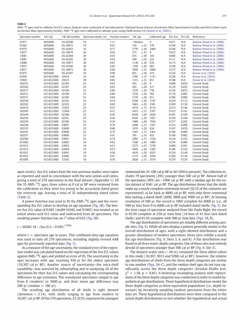
Table 2AMS-14C ages used to calibrate Asx D/L values. Analyses were conducted at two laboratories (National Ocean Sciences Accelerator Mass Spectrometry Facility and Keck Carbon CycleAccelerator Mass Spectrometry Facility). AMS-14C ages were calibrated to calendar years using CALIB version 5.0 (Stuiver et al. (2005)).

Specimen number 14C Lab 14C lab number Specimen depth (m) Fraction modern 14C age Calibrated age D/L Asx D/L Glx References

91071 NOSAMS OS-42389 10 1.11 NModern 0 0.071 N/A Barbour Wood et al. (2006)91062 NOSAMS OS-39672 10 0.91 745 ±35 378 0.160 N/A Barbour Wood et al. (2006)91075 NOSAMS OS-42453 10 0.71 2770 ±30 2484 0.246 N/A Barbour Wood et al. (2006)13077 NOSAMS OS-39670 30 0.95 375 ±35 0 0.072 N/A Barbour Wood et al. (2006)13081 NOSAMS OS-42384 30 0.93 555 ±30 183 0.083 N/A Barbour Wood et al. (2006)13087 NOSAMS OS-42385 30 0.93 590 ±25 222 0.111 N/A Barbour Wood et al. (2006)13088 NOSAMS OS-39671 30 0.87 1130 ±30 676 0.173 N/A Barbour Wood et al. (2006)13075 NOSAMS OS-43396 30 0.85 1350 ±50 883 0.160 N/A Barbour Wood et al. (2006)13071 NOSAMS OS-39673 30 0.68 3050 ±35 2808 0.273 N/A Barbour Wood et al. (2006)91077 NOSAMS OS-43397 10 0.90 855 ±50 474 0.143 N/A Krause et al. (2010)91050 UCI-KCCAMS 29524 10 0.82 1595 ±15 1151 0.228 N/A Krause et al. (2010)13050 UCI-KCCAMS 29522 30 0.85 1315 ±25 851 0.188 N/A Krause et al. (2010)182531 UCI-KCCAMS 62185 25 0.95 435 ±20 0 0.088 0.034 Current Study182542 UCI-KCCAMS 62187 25 0.93 585 ±20 217 0.129 0.052 Current Study182517 UCI-KCCAMS 62184 25 0.86 1210 ±20 738 0.154 0.072 Current Study182551 UCI-KCCAMS 62190 25 0.86 1250 ±20 782 0.178 0.083 Current Study182537 UCI-KCCAMS 62186 25 0.84 1370 ±20 911 0.206 0.089 Current Study182558 UCI-KCCAMS 62192 25 0.76 2160 ±20 1747 0.229 0.112 Current Study182502 UCI-KCCAMS 62183 25 0.65 3465 ±20 3341 0.269 0.136 Current Study182510 UCI-KCCAMS 72303 25 0.57 4510 ±15 4714 0.273 0.140 Current Study182505 UCI-KCCAMS 72304 25 0.51 5415 ±15 5787 0.313 0.161 Current Study182544 UCI-KCCAMS 62188 25 0.45 6450 ±20 6929 0.301 0.160 Current Study182556 UCI-KCCAMS 62191 25 0.44 6545 ±20 7057 0.330 0.168 Current Study182550 UCI-KCCAMS 62189 25 0.39 7480 ±20 7936 0.377 0.202 Current Study182528 UCI-KCCAMS 63897 25 0.78 2040 ±15 1597 0.212 0.098 Current Study182535 UCI-KCCAMS 63898 25 0.88 1070 ±20 634 0.167 0.076 Current Study182541 UCI-KCCAMS 63899 25 0.79 1925 ±15 1461 0.189 0.089 Current Study182557 UCI-KCCAMS 63900 25 0.91 785 ±25 425 0.140 0.062 Current Study182560 UCI-KCCAMS 63901 25 0.78 2005 ±15 1558 0.218 0.102 Current Study451002 UCI-KCCAMS 63902 10 0.83 1540 ±20 1089 0.195 0.080 Current Study451012 UCI-KCCAMS 63903 10 0.51 5375 ±25 5730 0.406 0.201 Current Study451013 UCI-KCCAMS 63904 10 0.53 5045 ±20 5383 0.346 0.165 Current Study451021 UCI-KCCAMS 63905 10 0.58 4410 ±20 4553 0.324 0.149 Current Study451022 UCI-KCCAMS 63906 10 0.67 3175 ±20 2958 0.269 0.120 Current Study451005 UCI-KCCAMS 72302 10 0.70 2820 ±15 2574 0.279 0.129 Current Study

277T.A. Dexter et al. / Quaternary Research 81 (2014) 274–283

open circles). Asx D/L values from the two previous studies were takenas reported and used in concordance with the new amino acid ratios,giving a total of 270 specimens in the final dataset (Appendix 1). Ofthe 35 AMS-14C ages, three valves at 0 cal yr BP were removed fromthe calibration as they were too young to be accurately dated giventhe reservoir age, leaving a total of 32 independently dated valves(Table 2).

A power function was used to fit the AMS-14C ages and the corre-sponding Asx D/L values to develop an age equation (Fig. 2B). The low-est Asx D/L value of 0.045 (shell# 91042 and 91065) was treated as aninitial amino acid D/L value and subtracted from all specimens. Theresulting power function has an r2 value of 0.92 (Fig. 2B):

t ¼ 60282:18 � Asx D=L−0:045ð Þ1:9594

where t = specimen age in years. This combined-data age equationwas used to date all 270 specimens, including slightly revised AARages for previously reported data (Fig. 3).

As ameasure of the age uncertainty, the standard error of the regres-sionmodel was calculated based on the regression of the Asx D/L valuesagainst AMS-14C ages and yielded an error of 9%. The uncertainty in theages increases with age, reaching 936 yr for the oldest specimen(10,307 cal yr BP). Another source of uncertainty—the intra-shellvariability—was assessed by subsampling and re-analyzing 26 of thespecimens for their Asx D/L values and calculating the correspondingdifference in age estimates. The reanalyzed specimens ranged in agefrom 0 (modern) to 5600 yr, and their mean age difference was298 yr (median = 186 yr).

The resulting age distribution of all shells is right skewed(skewness = 2.14), with shells ranging in age from modern to10,307 cal yr BP. Of the 270 specimens, 23 (8.5%) represent the youngest

centennial bin (0–100 cal yr BP or AD1850 to present). The collection in-cludes 79 specimens (29%) younger than 500 cal yr BP. Almost half ofthe specimens (49%) are b1000 cal yr BP, with a median age for the en-tire dataset of 1041 cal yr BP. The age distribution shows that the shellsmake up a nearly complete centennial record (92.5% of the centuries arerepresented) as far back as 4000 cal yr BP, with only three centennialbins lacking a dated shell (2600, 3800 and 3900 cal yr BP). At binningresolution of 500 yr, the record is 100% complete for 6000 yr (i.e., all500-yr bins from 0 to 6000 cal yr BP included dated shells; Fig. 3). Forthe time range of specimens analyzed from São Paulo Bight, the recordis 65.9% complete at 250-yr time bins (14 bins of 41 bins lack datedshells) and 81.0% complete with 500-yr time bins (Figs. 3A, B).

The age distributions of specimens are notably different among sam-ple sites (Fig. 4). While all sites display a pattern generally similar to theoverall distribution of ages, with a right-skewed distribution and agreater abundance of modern specimens, three sites exhibit a nearlyflat age distribution (Fig. 4; Sites 3, 4, and 8). A flat distribution wasfound in all threewater-depth categories. One of these siteswas entirelydevoid of specimens younger than 500 cal yr BP (Fig. 4; Site 3).

The deepest-water sites (N30 m) contained the three oldest valvesin this study (10,307, 9913 and 9288 cal yr BP); however, the relativeage distributions of shells from the three depth categories are similarto one another (Figs. 5A–C), and the median shell ages do not vary sig-nificantly across the three depth categories (Kruskal–Wallis test:χ2 = 1.58, p = 0.45). A bootstrap resampling analysis with replace-ment of the three depth categorieswas conducted in order tomodel hy-pothetical age distributions. These hypothetical distributions model thethree depth categories as three equivalent populations (i.e., depth in-variant) by iteratively sampling random specimens from the entiredata set. These hypothetical distributions were then compared to theactual depth distributions to test whether the hypothetical and actual

Figure 2. (A) Comparison between Asx and Glx D/L values for each shell analyzed in thisstudy. Five specimens (open circles) were considered outliers and rejected because the re-siduals of the major axis regression of D/L values against age exceeded 2σ deviation. (B) Ex-tent of Asx racemization (D/L) comparedwith theAMS-14C age of 32 specimens analyzed forboth Asx D/L and 14C. A power functionwas used to calibrate the rate of racemization to de-rive the age equation. Water depths of the collection site for each specimen are indicated.

Figure 3. Age distribution of the 270 analyzed specimens of S. casali. Ages were deter-mined using a single calibration equation calculated using 32 AMS-14C-dated shells thatwere also analyzed for amino acid racemization (Fig. 2B). Specimens range in age frommodern to N10,000 cal yr BP. Specimens were grouped into two different bin sizes (A)250 yr intervals, and (B) 500-yr intervals. The structure of the age frequency ismaintainedwhen the bin size is varied, showing this nearly continuous distribution through time.

278 T.A. Dexter et al. / Quaternary Research 81 (2014) 274–283

depth categories are equivalent as would be expected for specimenscollected from the same population (i.e., depth invariant) or whetherthe actual data are distinct from the hypothetical models (i.e., depth de-pendent). Median age, skewness, and kurtosis were used to classifyeach hypothetical depth category as these values describe the centraltendency and shape of the distribution. To compare the differences be-tween the three hypothetical depth categories at each iteration, thestandard deviation of mean ages, median ages, skewness, and kurtosiswere calculated. The standard deviation of these values for each itera-tionwas then recorded to create a distribution of hypothetical outcomesfrom random specimen selected from the samepopulation (Figs. 5D–E).The standarddeviation,mean ages,median ages, skewness, and kurtosisof the actual depth categories were then compared to the hypotheticalmodel (arrows in Figs. 5D–E). The three depth categories had a standarddeviation of median ages of 98 yr with a range of 186 yr (870 to1057 yr). The standard deviation of mean ages was 160 yr with arange of 300 yr (1442 to 1743 yr). The standard deviation of skewnessamong the depth categorieswas 0.60with a range of 1.13 (1.38 to 2.50).The standard deviation of kurtosis was 2.03with a range of 3.82 (1.74 to5.56). The actual values observed for the data are well within the rangeof expected standard deviations predicted by the hypothetical modelsof specimens pooled from the same population.

To assess the influence of depth on the rate of AAR, age equationswere calculated for the three depths forwhichAMS-14C ageswere avail-able (10 m, 25 m, and 30 m). Each of these depth-specific equationswas applied to the entire data set of amino acid ratios to derive threeseparate age distributions (Table 3). Multiple statistical metrics wereused to compare the ages attained from the depth-specific equationsto the combined equation to address the possible influence of depthon AAR rates (Table 3). The three depth-specific equations created age

distributions that were similar for the entire dataset and for the com-bined equation regardless of depth (Table 3).

While D/L Asx valueswere analyzed for all AMS-14C dated specimens,D/L values for other amino acids were available for only some of thosespecimens. These data were used to calculate calibrated age equationsfor Glx and Ala. The resulting ages are similar to those using Asx, despitefewer calibration points (Table 4). The distribution of Glx-inferred ageshas a similar structure to Asx (r2 = 0.9174), but the Glx age estimatesare younger than those obtained using the Asx calibration (Table 4).Ala-inferred ages are highly consistent with the Asx ages (r2 = 0.9274).Ser cannot be used for AAR geochronology because it typically reachesamaximumvalue of about 0.4, then decreaseswith age. Ser values are re-ported because they can be indicative of contamination. To further assessthe differences in amino acids, Asxwas reevaluated and a new calibrationcurve recalculated using only the AMS-14C-dated specimens for whichGlx andAlawas also available (n = 22). This newcalibrationwas appliedto date only the specimens for which other amino acid values were ana-lyzed on the valve (n = 195) to make the age distributions comparable(Table 4; Asx subset). The difference in ages for valves calibrated usingAsx (subset) versus Glx has a mean value of 379 yr (median = 217 yr).When comparing Asx (subset) to Ala, the mean difference in ages is429 yr (median = 345 yr).

Discussion

Geochronology and implications for future research

The AAR dated shells, collected from the taphonomically active zone(TAZ, sensu Davies et al., 1979), reveal a right-skewed temporal

Figure 4.Distribution of specimen ages by collection site for all siteswith 10 ormore specimens. Age distributions differ among sites.Whilemost are dominated by young shells frommostrecent centuries, a few of the sites include relatively few young shells (Sites 8 and 4) or completely lack (Site 3) modern specimens.

279T.A. Dexter et al. / Quaternary Research 81 (2014) 274–283

distribution that includes valves with long (multi-millennial) residencetimes (Fig. 3). The dated shells comprise a remarkably complete timeseries, with nearly every century represented by at least one specimen,back to 4000 cal yr BP (missing only the 2600 and 3800 and 3900 cal yrbins). Right-skewed age distributions including old shells near the sed-iment surface have been observed in many recent studies (Kowalewskiet al., 1998; Carroll et al., 2003; Kidwell et al., 2005; Kosnik et al., 2007),though the temporal range for thematerial analyzed here exceedswhathas been observed previously in other depositional settings (seeKowalewski, 2009 for a comparison of age distributions for variousspecies).

The dated shells were collected across a depth gradient from whichwe can assess whether temporal mixing varies significantly with waterdepth. Previous studies suggest that mean specimen age and extent oftime-averaging increase with increasing distance from shore (Flessaand Kowalewski, 1994). For this study, the specimen depth categorieswere coarsely grouped because samples from some depths includedonly a few specimens. Comparison of the age distributions based onthe three depth categories suggests similar scales and structures oftime-averaging. The non-parametric Kruskal–Wallis one-way analysisof variance suggests that the three depth assemblages were not signifi-cantly different (χ2 = 1.58, p = 0.45). Further, the age distributions of

Figure 5. Age distributions grouped by specimen collection depth. Depth categories include (A) shallow (b20 m), (B)moderate (20–30 m), and (C) deep (N30 m). Frequency is given as apercent of the total number (n) of specimens from each depth category. All bathymetric ranges display similar age distributions. A bootstrap analysis with replacement was conducted todetermine the potential age distribution of specimens sampled from the same population. The frequency of the standard deviation of themedian ages (D) and standard deviation of skew-ness (E) between the three depth categories was recorded for 1000 iterations of the bootstrap analysis. The arrows in panels D and E indicate the actual standard deviation of the medianand skewness for the three depth categories (standard deviation of actual median ages = 162 yr, standard deviation of actual skewness = 0.6163). The actual standard deviation ofme-dian and skewnesswas locatedwellwithin the potential values determined by the bootstrap analysis using specimens sampled from the same population. The bootstrap analysis failed todemonstrate that the three depth categories are significantly different from one another.

280 T.A. Dexter et al. / Quaternary Research 81 (2014) 274–283

shells from the three depth categories had similar skewness, median,mean, and kurtosis with low among-group standard deviations(Table 3). By using a bootstrap resampling method (see the Methodsand materials section), it was possible to further assess whether time-averaging varied significantly with depth by comparing the actualdepth distributions to resampled distributions in which any age valuefrom the entire dataset is possible regardless of depth. This bootstrap re-sampling tested the null hypothesis that the actual age distributionscame from the same, depth-invariant age distribution. The actual valuesfor the standard deviation of mean, median, skewness and kurtosis fellwithin the distribution of possible values as determined by the boot-strap resampling analysis, providing no statistical evidence for the sig-nificance of actual differences observed among the three depthcategories (Figs. 5D, E). Thus, time-averaging appears relatively

Table 3Summary of specimen ages calculated using depth-specific equations. Three age equations werAsx D/L values from all the valves of this study to determine the effect of depth on racemizatioculated from the ages of the entire dataset using the three depth-specific equations and were

AMS-14C sample depths Na Ab Xc r2d Mean age (cal y

10 m 10 35343.09 1.49 0.97876 202225 m 16 86071.83 1.81 0.96877 288430 m 6 41379.15 1.59 0.98177 1999All depths 32 60282.18 1.96 0.92398 1584

a Number of AMS 14C specimens at a given depth.b Rate constant of the power function.c Power exponent of D/L in the power function.d r2 fit of the power function to the AMS 14C ages.

comparable across the sampled bathymetric range, suggesting spatiallyuniform rates of accumulation and reworking for the surficial shellmaterial.

Whereas the age distributions are similar along the bathymetric gra-dient, there is notable variation from site to site. A few individual sitesreveal a paucity of modern material and one of the sites (Site 3) iscompletely devoid of modern specimens (Fig. 4). This notable localpatchiness in time-averaging processes is difficult to interpret. Theshape of age distributions and the scale of time-averaging are affectedby multiple factors (sedimentation rates, depth and frequency ofreworking, intensity of destructive taphonomic processes, biologicalproductivity, and intrastratal biological activity),whichmayhave variedlocally contributing to the observed variation in age structures from onesite to another.

e calculated based on the AMS-14C ages on valves of three depths and were applied to then rates at this locality. Mean, median, standard deviation, skewness and kurtosis were cal-then compared to the combined age equation.

r BP) Median age (cal yr BP) Standard deviation Skewness Kurtosis

1604 1678 1.44 2.652011 2880 1.92 4.841526 1762 1.59 3.281033 1711 2.14 6.06

Table 4Summary of specimen ages calculated using different amino acids. A subset of valves with both aspartic acid and glutamic acid valueswas used to determine a new Asx equation that wascomparable to the other amino acids.

Amino acid Na Ab Xc r2d Lowest D/L value Maximum age(cal yr BP)

Mean age(cal yr BP)

Median age(cal yr BP)

Standard deviation Skewness Kurtosis

Asx 32 60282.18 1.96 0.9240 0.045 10,307 1584 1033 1711 2.14 6.06Glx 22 147354.40 1.72 0.9576 0.020 8529 1501 954 1598 1.98 4.48Ala 22 39267.01 1.54 0.9835 0.022 10,630 1522 812 1837 2.25 5.93Asx subset 22 51008.09 1.79 0.9269 0.050 9975 1806 1209 1783 1.99 5.05

a Number of AMS 14C specimens with corresponding AAR values.b Rate constant of the power function.c Power exponent of D/L in the power function.d r2 fit of the power function to the AMS 14C ages.

281T.A. Dexter et al. / Quaternary Research 81 (2014) 274–283

The unusually old age of our specimens from the study area, collect-ed at or near the sediment surface, is unexpected given that the valves ofS. casali are small and thin (see also Valentine et al., 2006). The valvescollected for this study had little taphonomic alteration with limitedabrasion, dissolution, and minor epibiont encrustation. Such minor al-terationwould not be expected for valves that have resided continuous-lywithin the TAZ at or slightly under the sediment surface for thousandsof years. The prevalence of relativelywell preserved valves suggests thatthese specimens were buried for most of their post-mortem history, aseven short exposure above the sediment surfacewould quickly degradesuch thin, fragile valves leaving no material behind to analyze. Age-frequency distributions of the thicker specimens of the calcitic brachio-pod Bouchardia rosea from this same locality reveal a similar right-skewed age structure with a similar age range (from 0 to 8000 cal yrBP), despite the notably smaller sample size (n = 103) (Carroll et al.,2003; Krause et al., 2010).

The similar age distribution for these two taphonomically distinctbiominerals suggests that extrinsic factors rather than intrinsic shellcharacteristics are responsible for controlling the scale and structure oftime-averaging in the study area. As noted by multiple authors (see ref-erences in Mahiques et al., 2011), the southwestern Atlantic upper mar-gin, including the São Paulo Bight, is marked by low sedimentation rates.Hence, the most likely explanation for our results is shell burial belowthe TAZ with minimal intermittent re-exposure into this destructivezone, which conforms to interpretations of extensive time-averagingproposed previously (Flessa et al., 1993; L. Martin et al., 1996; R.E.Martin et al., 1996; Meldahl et al., 1997; Kowalewski et al., 1998;Carroll et al., 2003; Olszewski, 2004). Valves can be buried under the sed-iment rapidly (particularly infaunal bivalves such as S. casali) and ex-humed intermittently back to the surface (Clifton, 1971; Parsons-Hubbard et al., 1999). With the low exhumation and turnover rates,older valves can be preserved for long periods of time. Thus the extensivetime-averaging documented here may typify other marine sediment-starved settings regardless of the type of biomineralized material.

The dating efforts reported here demonstrate that the surficial accu-mulations from the southeast Brazilian Bight provide multi-millennialrecords suitable for reconstructing long-term environmental change.Geochemical analyses of biomineralized shell materials provide multi-ple proxies (e.g., trace elements, stable isotopes) that reflect the condi-tions in which the shell-secreting organisms lived. As geochemicalmethods and resolution continue to improve, and dating techniques be-come more efficient and inexpensive, biomineralized materials fromtime-averaged shell accumulations should provide an increasingwealthof environmental proxy data.

Methodological implications

WhenAMS-14C ages are plotted against AsxD/L values for data pooledacross all sites, the two data series are tightly correlated (Fig. 2B). Theconsistent racemization rates observed here across a depth gradient arenot unexpected given that all sampled sites, regardless of their depth,occur within the same fully mixed water mass and are unlikely to have

experienced a notable temperature gradient (Campos et al., 2000). In ad-dition, the spatial uniformity in racemization rates suggests that theshallower sites could not have been subaerially exposed because suchevents would notably change the thermal history of the affected speci-mens andprevent an effective application of a single calibration equation.This again is not unexpected in our study area. All sites have remainedsubmerged since the Holocene post-glacial transgression, and sea levelhas remained relatively unchanged for the past 5000 yr (L. Martin et al.,1996; R.E. Martin et al., 1996; Angulo and Lessa, 1997; Angulo et al.,1999, 2004; Lessa et al., 2000; Baker et al., 2001) providing potentially fa-vorable conditions for developing a reliable single calibration for sitesvarying in water depth. Indirectly, thus, the results provide an indepen-dent confirmation of oceanographic and sea-level histories of the regionderived previously using other lines of evidence (references cited above).

To further assess the use of a single calibration, three depth-specificcalibration equations were calculated from the three depths for whichAMS-14C ages were available. These three equations were applied tothe entire dataset and the age distributions were compared to the sin-gle, depth invariant equation (Table 3). The three depth-specific calibra-tions produced age distributions that were similar in structure to thepooled calibration as demonstrated by a number of statistical metrics(Table 3).

Considering multiple sites at multiple depths concurrently ratherthan separately reduces the needed number of AMS-14C ages, as site-specific calibrations are no longer necessary. The use of a single calibra-tion equation could average values and obscure real differences be-tween sites and depths. As demonstrated in this study with the threedepth-specific AMS-14C calibrations, the use of the single calibrationdid not change the overall age distributions noticeably from those calcu-lated based on depth (Table 3). This suggests that the lack of differencein time-averagingbetweendepths is real and not an artifact of the singlecalibration equation. Further, the use of a single calibration formula forthe entire region did not prevent us from detecting local, site-to-sitevariability in age distributions of dated shells (Fig. 4). In study areaswith greater spatial variability in thermal history, more intensivedepth-specific AMS-14C dating would be necessary to calibrate AARrates. However, for fully mixed water masses unaffected by substantiallocal sea-level changes, a single calibration for multiple sites appearsto suffice. Because AMS-14C ages are the more cost-prohibitive aspectof large geochronological studies, reducing the number of analyses re-quired to calibrate AAR rates facilitates the development of large geo-chronological datasets.

Summary and conclusions

Using amino acid racemization ratios calibrated against AMS-14Cages (n = 32), 270 S. casali valves were dated individually and age-frequency distributions were assembled for 14 sites within the SãoPaulo Bight, southeastern Brazil (Fig. 1). Specimens range in age frommodern to 10,307 cal yr BP. For most sites, and for pooled data, age dis-tributions are right skewed and provide a nearly continuous geochrono-logical record for the past 4000 yr at the centennial scale of resolution

282 T.A. Dexter et al. / Quaternary Research 81 (2014) 274–283

(92.5%). At the millennial scale of resolution, the dated shells provide anearly complete record for the entire Holocene (90%). Due to limitedtransport, intermittent exposure and burial and a spatially consistentthermal history throughout the study area, a single calibration can beapplied to all specimens measured for AAR.

Periodic burial of modern material throughout the Holocene, withlow exhumation and turnover rates of older valves buried in the shal-low subsurface, allowed for near-surficial survival of many old speci-mens providing a long and remarkably continuous time series ofdated shells. Shelfal settings characterized by low sedimentation ratesand stable relative sea level during the Holocene highstand facilitatepreservation and mixing of shelly specimens from multiple millennia.These conditions should be present in many marine settings increasingthe likelihood of assembling long time-series of dated shells for a varietyof biomineralized materials, which can then be used as a source of geo-chemical proxy data for tracking regional environmental and climatictrends throughout the Holocene. Use of geochemical data frombiomineralized materials as a proxy for environmental conditions isan established and increasingly widespread strategy in late Quaternarystudies. This and previous studies demonstrate that AAR dating of surfi-cial shell accumulations allows for assembling extensive time series ofbiomineral solids suitable for paleoenvironmental and paleoclimaticstudies spanning multi-centennial to multi-millennial time scales.Shells that lay on modern seafloors do not just record the present, butrepresent a wealth of past data that can span many millennia.

Acknowledgments

This study was supported by National Science Foundation grantsOCE-0602375 (Virginia Tech, Savannah River Ecology Laboratory ofthe University of Georgia, and Northern Arizona University), EAR-0125149 (Virginia Tech, GeorgeWashington University, and Universityof Delaware), and EAR-1234413 (Northern Arizona University), the Pe-troleum Research Fund of the American Chemical Society (40735-AC2),and the São Paulo State Science Foundation [FAPESP] (00/12659-7, SãoPaulo State University). Funding was also provided from the Depart-ment of Geosciences at Virginia Tech (for TAD, RAK, SLBW, and JWH)and Jon L. and Beverly A. Thompson Endowment Fund (FloridaMuseumof Natural History, University of Florida).We also thank Silvia Helena deMello e Souza, Oceanographic Institute, University of Sao Paulo, for pro-viding samples. The authors thank Thomas Olszewski, Ashok K. Singhvi,Derek Booth, and an anonymous reviewer for their comments on thismanuscript.

Appendix A. Supplementary data

Supplementary data to this article can be found online at http://dx.doi.org/10.1016/j.yqres.2013.12.007.

References

Anderson, L.C., Sen Gupta, B.K., McBride, R.A., Byrnes, M.R., 1997. Reduced seasonality ofHolocene climate and pervasive mixing of Holocene marine section: NortheasternGulf of Mexico shelf. Geology 25, 127–130.

Angulo, R.J., Lessa, J.C., 1997. The Brazilian sea-level curves: a critical review with empha-sis on the curves from the Paranaguá and Cananéia regions. Marine Geology 140,141–166.

Angulo, R.J., Giannini, P.C.F., Suguio, K., Pessenda, L.C.R., 1999. Relative sea-level changesin the last 5500 years in southern Brazil (Laguna-Imbituba region, Santa CatarinaState) based on vermetid 14C ages. Marine Geology 159, 323–339.

Angulo, R.J., Lessa, J.C., de Souza,M.C., 2004. A critical review ofmid- to late-Holocene sea-level fluctuations on the eastern Brazilian coastline. Quaternary Science Reviews 25,486–506.

Angulo, R.J., de Souza, M.C., Reimer, P.J., Sasaoka, S.K., 2005. Reservoir effect of the South-ern and Southeastern Brazillian Coast. Radiocarbon 47, 67–73.

Baker, R.G.V., Haworth, R.J., Flood, P.G., 2001. Warmer or cooler late Holocene marinepalaeoenvironments? Interpreting southeast Australian and Brazilian sea-level changesusing fixed biological indicators and their δ18O composition. Palaeogeography,Palaeoclimatology, Palaeoecology 168, 249–272.

Barbour Wood, S.L., Krause Jr., R.A., Kowalewski, M., Wehmiller, J., Simões, M.G.,2006. Aspartic acid racemization dating of Holocene brachiopods and bivalvesfrom the southern Brazilian shelf, South Atlantic. Quaternary Research 66,323–331.

Campos, E.J.D., Lentini, C.A.D., Miller, J.L., Piola, A.R., 1999. Interannual variability of the seasurface temperature in the South Brazil Bight. Geophysical Research Letters 26,2061–2064.

Campos, E.J.D., Velhot, D., da Silveira, I.C.A., 2000. Shelf break upwelling driven by BrazilCurrent cyclonic meanders. Geophysical Research Letters 27, 751–754.

Carroll, M., Kowalewski, M., Simões, M.G., Goodfriend, G.A., 2003. Quantitative estimatesof time-averaging in brachiopod shell accumulations from a modern tropical shelf.Paleobiology 29, 381–402.

Clarke, S.J., Murray-Wallace, C.V., 2006. Mathematical expressions used in amino acid ra-cemization geochronology—a review. Quaternary Geochronology 1, 261–278.

Clifton, H.E., 1971. Orientation of empty pelecypod shells and shell fragments in quietwater. Journal of Sedimentary Petrology 41, 671–682.

Collins, M.J.,Waite, E.R., van Duin, A.C.T., 1999. Predicting protein decomposition: the caseof aspartic-acid racemization kinetics. Philosophical Transactions of the Royal Societyof London. Series B: Biological Sciences 354, 51–64.

Davies, D.J., Powell, E.N., Stanton Jr., R.J., 1979. Relative rates of shell dissolution and netsediment accumulation‐a commentary: can shell beds form by the gradual accumu-lation of biogenic debris on the sea floor? Lethaia 22, 207–212.

Demarchi, B., Williams, M.G., Milner, N., Russell, N., Bailey, G., Penkman, K., 2011. Aminoacid racemization dating of marine shells: a mound of possibilities. Quaternary Inter-national 239, 114–124.

Doello-Jurado, M., 1949. Dos nuevas especies de bivalvos marinos. ComunicacionesZoologicas del Museo de Historia Natural de Montevideo 3, 1–8.

Flessa, K.W., 1998. Well-traveled cockles: shell transport during the Holocene transgres-sion of the southern North Sea. Geology 26, 187–190.

Flessa, K.W., Kowalewski, M., 1994. Shell survival and time-averaging in nearshoreand shelf environments: estimates from the radiocarbon literature. Lethaia 27,153–165.

Flessa, K.W., Cutler, A.H., Meldahl, K.H., 1993. Time and taphonomy: quantitative esti-mates of time-averaging and stratigraphic disorder in a shallow marine habitat. Pa-leobiology 19, 266–286.

Goodfriend, G.A., 1992. Rapid racemization of aspartic acid inmollusc shells and potentialfor dating over recent centuries. Nature 357, 399–401.

Goodfriend, G.A., Stanley, D.J., 1996. Reworking and discontinuities in Holocene sedimen-tation in the Nile Delta: documentation from amino acid racemization and stable iso-topes in mollusk shells. Marine Geology 129, 271–283.

Goodfriend, G.A., Brigham-Grette, J., Miller, G.H., 1996. Enhanced age resolution of themarine Quaternary record in the arctic using aspartic acid racemization dating of bi-valve shells. Quaternary Research 45, 176–187.

Hammer, Ø., Harper, D.A.T., Ryan, P.D., 2001. PAST: paleontological statistics softwarepackage for education and data analysis. Palaeontologia Electronica 4, 1–9 (http://palaeo-electronica.org/2001_1/past/issue1_01.htm).

Hill, R.L., 1965. Hydrolysis of proteins. In: Anfinsen, C.B., Anson, M.L., Edsall, J.T., Richards,F.M. (Eds.), Advances in Protein Chemistry, vol. 20. Academic Press, pp. 37–107.

Hughen, K.A., Baillie, M.G.L., Bard, E., Bayliss, A., Bertrand, C.J.H., Blackwell, P.G., Buck, C.E.,Burr, G.S., Cutler, K.B., Damon, P.E., Edwards, R.L., Fairbanks, R.G., Friedrich, M.,Guilderson, T.P., Kromer, B., McCormac, F.G., Manning, S.W., Ramsey, C.B., Reimer,P.J., Reimer, R.W., Remmele, S., Southon, J.R., Stuvier, M., Talamo, S., Taylor, F.W.,van der Plicht, J., Weyhenmeyer, C.E., 2004. Marine04 marine radiocarbon age cali-bration, 0–26 cal kyr BP. Radiocarbon 46, 1059–1086.

Kaufman, D.S., Manley, W.F., 1998. A new procedure for determining DL amino acid ratios infossils using reverse phase liquid chromatography. Quaternary Science Reviews 17,987–1000.

Kidwell, S.M., Best, M.M.R., Kaufman, D.S., 2005. Taphonomic trade-offs in tropical marinedeath assemblages: differential time-averaging, shell loss, and probable bias insiliciclastic vs. carbonate facies. Geology 33, 729–732.

Kosnik, M.A., Kaufman, D.S., 2008. Identifying outliers and assessing the accuracy ofamino acid racemization measurements for geochronology: II. Data screening. Qua-ternary Geochronology 3, 328–341.

Kosnik, M.A., Hua, Q., Jacobsen, G.E., Kaufman, D.S., Wüst, R.A., 2007. Sediment mixing andstratigraphic disorder revealed by the age-structure of Tellina shells in Great BarrierReef sediment. Geology 35, 811–814.

Kosnik, M.A., Kaufman, D.S., Hua, Q., 2008. Identifying outliers and assessing the accuracyof amino acid racemization measurements for geochronology: I. Age calibrationcurves. Quaternary Geochronology 3, 308–327.

Kowalewski, M., 2009. The youngest fossil record and conservation biology: Holoceneshells as eco-environmental recorders. In: Dietl, G.P., Flessa, K.W. (Eds.), ConservationPaleobiology: Using the Past to Manage for the Future. The Paleontological SocietyPapers, 15, pp. 1–23.

Kowalewski, M., Goodfriend, G.A., Flessa, K.W., 1998. High-resolution estimates of temporalmixing within shell beds: the evils and virtues of time-averaging. Paleobiology 24,287–304.

Krause Jr., R.A., Barbour Wood, S.L., Kowalewski, M., Kaufman, D.S., Romanek, C.S.,Simões, M.G., Wehmiller, J.F., 2010. Quantitative comparisons and models oftime-averaging in bivalve and brachiopod shell accumulations. Paleobiology36, 428–452.

Lessa, G.C., Angulo, R.J., Giannini, P.C., Araujo, A.D., 2000. Stratigraphy and Holocene evo-lution of a regressive barrier in South Brazil. Marine Geology 165, 87–108.

Mahiques, M.M., Sousa, S.H.M., Burone, L., Nagai, R.H., Silveira, I.C.A., Figueira, R.C.L.,Soutelino, R.G., Ponsoni, L., Klein, D.A., 2011. Radiocarbon geochronology of the sedi-ments of the São Paulo Bight (southern Brazilian upper margin). Anais da AcademiaBrasileira de Ciências 83, 817–834.

283T.A. Dexter et al. / Quaternary Research 81 (2014) 274–283

Martin, L., Suguio, K., Flexor, J.M., Dominguez, J.M.L., Bittencourt, A.C.S.P., 1996a. Quater-nary sea-level history and variation in dynamics along the central Brazilian coast:consequences on coastal plain construction. Anais de Academia Brasileirade Ciências68, 303–354.

Martin, R.E., Wehmiller, J.F., Harris, M.S., Liddel, W.D., 1996b. Comparative taphonomy ofbivalves and foraminifera from Holocene tidal flat sediments, Bahia la Choya, Sonora,Mexico (northern Gulf of California): taphonomic grades and temporal resolution.Paleobiology 22, 80–90.

McCormac, F.G., Hogg, A.G., Blackwell, P.G., Buck, C.E., Higham, T.F.G., Reimer, P.J., 2004.SHCal04 Southern hemisphere calibration 0–11.0 cal kyr BP. Radiocarbon 46,1087–1092.

Meldahl, K.H., Flessa, K.W., Cutler, A.H., 1997. Time-averaging and postmortem skeletalsurvival in benthis fossil assemblages: quantitative comparisons among Holocene en-vironments. Paleobiology 23, 207–229.

Miller, G.H., Kaufman, D.S., Clarke, S.J., 2013. Amino acid dating, In: Elias, S.A. (Ed.), 2ndedition. Encyclopedia of Quaternary Science, volume 1. Elsevier, Amsterdam,pp. 37–48.

Narchi, W., Domaneschi, O., 1977. Semele casali— Jurado, 1949 (Mollusca, Bivalvia) in theBrazilian littoral. Studies on Neotropical Fauna and Environment 12, 263–272.

Olszewski, T.D., 2004. Modeling the influence of taphonomic destruction, reworking, andburial on time-averaging in fossil accumulations. Palaios 19, 39–50.

Parsons-Hubbard, K.M., Callender, W.R., Powell, E.N., Brett, C.E., Walker, S.E., Raymond,A.L., Staff, G.M., 1999. Rates of burial and disturbance of experimentally-deployedmolluscs: implications for preservation potential. Palaios 14, 337–351.

R Development Core Team, 2008. R: a language and environment for statistical comput-ing. R Foundation for Statistical Computing, Vienna, Austria3-900051-07-0 (URLhttp://www.R-project.org).

Stuiver, M., Reimer, P.J., Reimer, R.W., 2005. CALIB 5.0.2, Radiocarbon calibration program.http://calib.qub.ac.uk/calib/.

Valentine, J.W., Jablonski, D., Kidwell, S., Roy, K., 2006. Assessing the fidelity of the fossilrecord by using marine bivalves. Proceedings of the National Academy of Science103, 6599–6604.

Wehmiller, J.F., York, L.L., Bart, M.L., 1995. Amino-acid racemization geochronology ofreworked Quaternary mollusks on U.S. Atlantic coast beaches: implications forchronostratigraphy, taphonomy, and coastal sediment transport. Marine Geology124, 303–337.

Zhao, M., Bada, J.L., Ahern, T.J., 1989. Racemization rates of asparagine-aspartic acid resi-dues in lysozyme at 100 ºC as a function of pH. Bioorganic Chemistry 17, 36–40.