Hab in the MAB: Characterizing Black Sea Bass Habitat

in the Mid-Atlantic Bight

Final Report to the Atlantic Coastal Fish Habitat Partnership (ACFHP) May 2019

Bradley G. Stevens*, Cara Schweitzer**, and Andre Price***

University of Maryland Eastern Shore, Princess Anne, MD, 21853 * bgstevens@umes.edu

**cara.schweitzer42@gmail.com

***andre.price@noaa.gov

2

Acknowledgements This study was conducted by faculty and students at the University of Maryland Eastern Shore. We would not have been able to conduct this work without the assistance of many people. We would especially like to thank Captain J. Kogon of the OCDiveBoat, and fellow divers B. McMahon, A. Sterling, E. Gecys, and C. Coon for assistance with diving. Scuba diving and dive training was conducted under AAUS guidelines and the supervision of L. Burke and J. Dykman, Dive Safety Officers for the University System of Maryland. Angling support was provided by Capt. C. Mizurak of the Angler, and fellow fisher-students I. Fenwick, N. Coit, I. Oliver, O. Scott Price, J. Rice, and N. Olsen. I. Fenwick assisted greatly with fish capture, dissection, and stomach content analysis during summer of 2017 as an intern with the National Science Foundation Research Experiences for Undergraduates program at UMES. Funding for this project was provided by the Mid-Atlantic Fisheries Management Council, via a competitive award from the Atlantic Coast Fish Habitat Partnership. Funding for graduate student support was provided by the National Oceanic and Atmospheric Administration, Office of Education Educational Partnership Program award numbers NA11SEC4810002 and NA16SEC4810007. Chapters 1 and 2 of this work were submitted in partial completion of the PhD Dissertion for Cara S. Schweitzer at UMES. Chapter 3 of this work was submitted in partial completion of the MS Degree for Andre L. Price at UMES.

The contents of this report are solely the responsibility of the award recipient and do not necessarily represent the official views of the U.S. Department of Commerce, National Oceanic and Atmospheric Administration.

3

Introduction and Summary of Results The mid-Atlantic Bight (MAB) stretches from North Carolina to Massachusetts but is poorly studied, especially the nearshore regions of the Delaware, Maryland, and Virginia (Delmarva) peninsula. The nearshore continental shelf is composed primarily of unconsolidated sediments consisting of sand, silt, shells, and small gravels. Bedforms consist mainly of sand waves, small hills, and gullies created by ancient riverbeds, with rare outcroppings of rock, consolidated mud, and clay. There is very little hard bottom in the area. The distribution of habitats in the Delmarva MAB is poorly known, although some recent surveys have produced information on the bottom characteristics within the Maryland WEA. Seafloor sediments in the Delmarva region are characterized by large expanses of sand and shell, with widely scattered hard-bottom outcrops. These outcrops form small biological oases among a sandy seafloor desert, and are populated by sedentary invertebrate organisms that create structured habitat. Sedentary organisms are also present on anthropogenic debris (mostly shipwrecks). Numerous artificial reefs have been built in the region to enhance fishing and diving opportunities.

The nearshore continental shelf in this area is inhabited by several economically valuable species, including Tautog Tautoga onitis, Croaker Micropogonias undulatus, American Lobster Homarus americanus, summer flounder Paralichthys dentatus, and Black Sea Bass Centropristis striata. The most valuable inshore fishery is for black sea bass (BSB), which are considered a data poor species, due to a paucity of biological information regarding reproduction, age, growth, habitat preference, and mortality. Black sea bass are targeted by both recreational and commercial fisheries in equal measure, and the majority of commercial black sea bass landings are captured via fish traps. Commercial fish traps are often deployed on or near benthic structured habitat where economically valuable species aggregate. Recreational fishing is also mostly targeted on the many wrecks, artificial reefs, and natural bottom areas that are widely scattered throughout the region.

The MAB has become a proposed focal area for wind-power development, and wind energy areas (WEAs) have been designated offshore most of the coastal states including Maryland. Future development of wind power will affect bottom habitat in ways that are unknown, but the WEAs have been designed to avoid the most important habitats and fishing areas in the region. However, there is little information on habitat preferences of black sea bass, and how fishing or wind power development will affect the fish and their habitats. To understand the impacts of fishing or wind power development on black sea bass, we need a better understanding of the distribution and composition of benthic habitats in the MAB, and their importance to fish abundance, which is currently unknown.

Black sea bass Centropristis striata (BSB) are a carnivorous, primarily benthic fish that range from the Gulf of Maine to the Gulf of Mexico. Atlantic populations are separated into northern and southern stocks at Cape Hatteras, NC, and are considered a separate sub-species (Centropristis striata striata) from their Gulf of Mexico counterparts (Centropristis striata melana). Northern stock BSB perform seasonal migrations, residing in coastal waters in spring and summer months, then move to deeper waters near the continental shelf in the late fall through winter. BSB are protogynous hermaphrodites, with some individuals changing sex from female to male between 1 and 8 years of age. Common prey items for BSB include amphipods, decapods, bivalves, and small fish. Black sea bass tend to reside at sites with high rugosity at depths <28 m, that are largely associated with hard structure such as corals, mussel beds, and hard-bottom habitats or “reefs”. During the summer, fish show some site fidelity to these

4

habitats. Currently, there are few studies that describe the habitat characteristics of BSB, or their feeding dynamics, and how these two aspects of their biology are related.

This research project, designated “Hab in the MAB”, was designed to answer some of these questions. The original objectives were to:

1) Determine the preference of BSB for particular habitats by assessing their abundance, size structure, and feeding ecology within natural and artificial reefs;

2) Improve the understanding of benthic habitat structure by quantitatively assessing biodiversity, rugosity, and other habitat characteristics of natural and artificial reefs;

3) Determine if reduced fragmentation and increased connectivity of habitats increases fish recruitment, by experimentally manipulating corridors between isolated habitat patches.

During the course of the research, these goals were restructured into three specific sub-projects, and several minor ones as follows:

1. Determine the composition of biogenic structure on benthic habitat patches and the relationship to fish abundance, by

a. Estimating relative cover of fouling organisms and fish abundance at different types of reefs, and

b. Exploring the relationship between benthic diversity and fish abundance. 2. Investigate how seascape connectivity affects fish abundance, by

a. Establishing a small stepping-stone corridor connecting two existing reefs, and b. Monitoring changes in abundance of fish on the experimental and control reefs

before and after deployment; 3. Determine the dietary habits of black sea bass and their trophic relationships, by

a. Estimating trophic position using stable isotope analysis, and b. Comparing food habits between fish caught at artificial and natural reefs, and

during NOAA surveys.

Summary of Results Chapter 1: Habitat structure and fish preference

From 2016 through 2018, we investigated the interactions between black sea bass and their habitats at over a dozen artificial and natural reefs in the Delmarva MAB using a variety of techniques. At each of these reefs, we estimated fouling community composition using quadrat sampling with a digital camera and ¼ m2 frame along linear transects. We also estimated fish abundance using digital video cameras set on tripods, and by strip-transect censusing. Quadrat and video sampling were conducted both within the structured habitats and on nearby open-sand bottoms for comparison. Surveys of benthic habitats showed that the predominant marine biogenic structures in the Delmarva MAB are comprised of multiple species including northern stone coral Astrangia poculata, sponge Cliona celata, blue mussels Mytilus edulis, various hydroids (i.e. Tubularia sp., Obelia sp., Campanularia sp.), and gorgonian corals, putatively identified as sea whips Leptogorgia virgulata. Sea whips are one of the most prominent structure-forming invertebrates, and are responsible for most of the vertical structure above habitat baselines. Fish abundance at the studied sites was compared to the relative abundance of all other habitat-forming organisms present. Fish abundance was significantly correlated only with the relative abundance of sea whip corals, but not with abundance of any other species, or to total coverage of biogenic structure. Sea whips are ‘autogenic engineers’ (i.e. they create

5

biogenic structure) that add complexity to benthic habitats by altering the environment with their own physical structures. Previous studies (Schweitzer et al, 2018) have shown that 50% of commercial fish traps come into contact with emergent epifauna during deployment or recovery, including sea whip corals, often resulting in damage or breaking of corals. Assessment of sea whip condition (as a damage index) at our study sites showed that sea whip corals on artificial reefs off the Delmarva coast exhibited minor levels of degradation that did not differ significantly among study sites.

Chapter 2. Seascape Connectivity and Fish Abundance

To determine if increasing seascape connectivity increases fish abundance on isolated habitat patches, we used a Before-After-Control-Impact (BACI) experimental design. In 2016, we constructed a stepping-stone corridor (the ‘Impact’) connecting two established sections of an artificial reef (the Impact site). A similar, nearby, two-section reef was designated as the Control site. Both the Control and Impact site consisted of two structured components (parts of shipwrecks) separated by 20 or 120 m, respectively, of unstructured, open sand bottom. Fish abundance was estimated by conducting stationary video surveys during three sampling seasons for one year Before Impact and one year After Impact at both the Control and Impact sites, and on both the structured and unstructured components. Prior to Impact, fish were more abundant at the Impact than at the Control site, both sites showed seasonal variation in abundance, and fish were completely absent from unstructured bottom at both sites. After Impact, fish abundance increased significantly only at the (previously) unstructured portion of the Impact site (where the reef was built), but did not change at any of the structured portions of either site, or at the unstructured portion of the Control site. Furthermore, fish were observed on the corridor structure during all three sampling periods. Results suggest that corridor construction increased habitat availability for fish at the Impact site, without drawing fish away from nearby sites. This small-scale study demonstrated that increasing connectivity via corridor construction may be an effective method to enhance available habitat in marine ecosystems.

Chapter 3. Feeding Ecology of Black Sea Bass at Natural and Artificial Reefs

We sampled BSB at selected natural and artificial reefs near Ocean City, MD in 2016 and 2018, using hook-and-line angling to determine if reef type influenced length frequency, sex ratios, diets, and stable isotope ratios of ∂12C/∂13C and ∂14N/∂15N in liver, muscle, and mucus. BSB caught by angling were compared to a NOAA dataset of trawl-caught BSB spanning 2000-2016. There were no significant differences in size, age, or sex composition between fish at natural and artificial habitats. The primary prey items of BSB by proportion and frequency of occurrence were crustaceans (primarily Cancer crabs) at both artificial and natural sites and among the NOAA samples. Values of ∂15N and ∂13C differed between habitat types in liver and muscle, but not in mucus. This study showed that natural and artificial reefs are ecologically similar for Black Sea Bass caught near Ocean City, MD, but subtle differences in diet between reef types suggest that their physical form may affect access of fish to different prey items. Conclusions and Recommendations Previous studies suggesting that BSB are associated with “course-grained” material are but a crude approximation of habitat. The results of this project confirm that black sea bass are tightly structure-oriented, and primarily occur within <1 m of hard bottom substrata with substantial vertical and biological structure that includes the presence of gorgonian corals, aka sea whips.

6

While BSB did occur near newly placed structures with little overgrowth, abundance at most sites was significantly correlated with density of sea whips, but not of any other species. Increasing the presence of structured habitat, by placement of artificial structures, resulted in an increase in abundance of BSB, without detracting from nearby structures. Diets of BSB appear to derive mostly from areas surrounding reefs, rather than among them, and differ little based on the type of reef or other source. However, the structure and extent of reefs may have a minor impact on diet due to availability of different food sources. Nonetheless, this indicates that habitat selection is probably not associated with proximity to food sources, but is more likely to be associated with actual physical structure that provides other biological benefits, such as protection from predation, optimization of reproductive opportunities, or stress reduction.

With regard to future alteration of marine habitats in the MAB, we suggest that artificial reefs should be constructed out of solid structures with appropriately scaled interstitial space, rather than concrete blocks, pipe, or steel structures that are subject to degradation, subsidence, or disintegration. We also predict that construction or installation of wind power turbines will likely provide abundant hard structure supporting invertebrate fouling communities that black sea bass and other fish prefer as habitat. Increasing the availability of such artificial habitats in the MAB, and including some in protected areas, will likely have positive benefits for the regional population of black sea bass.

7

Chapter 1. The Relationship Between Fish Abundance and Community Structure on Artificial Reefs in the Mid-Atlantic Bight, and the Importance of Gorgonian Sea Whip Corals (Leptogorgia sp.) Adapted from: Schweitzer, C. C., and B. G. Stevens. in review. The importance of soft coral sea

whips (Leptogorgia sp.) to fish abundance on artificial reefs in the Mid-Atlantic Bight. PeerJ.

Abstract Autogenic engineers (i.e. biogenic structure) add to habitat complexity by altering the environment by their own physical structures. The presence of autogenic engineers is correlated with increases in species abundance and biodiversity. Biogenic structural communities off the coast of Delaware, Maryland, and Virginia (Delmarva) are comprised of multiple species including sea whips (putatively identified as Leptogorgia virgulata), northern stone coral Astrangia poculata, sponge Cliona celata, blue mussels Mytilus edulis, and various hydroids (i.e. Tubularia sp., Obelia sp., Campanularia sp.). Sea whips are soft corals that provide the majority of vertical height to benthic structure off the coast of the Delmarva peninsula. The mid-Atlantic bight is inhabited by several economically valuable fishes; however, data regarding habitat composition, habitat quality, and fish abundance are scarce. We collected quadrat and sea whip images from 12 artificial reef sites (i.e. shipwrecks) to determine proportional coverage of biogenic structures and to assess habitat health, respectively. Underwater video surveys were used to estimate fish abundances on the 12 study sites and determine if fish abundance was related to biogenic coverage and habitat health. Our results showed that higher fish abundance was significantly correlated with higher proportional sea whip coral coverage, but was not related to other species or total coverage of biogenic structure. Assessment of sea whip condition (as a damage index) showed that sea whip corals on artificial reefs off the Delmarva coast exhibited minor signs of degradation that did not differ significantly among study sites.

Introduction Structurally complex habitats, such as cobble and rock reefs, and natural or artificial reefs, are profoundly important for fish and crustaceans by providing spatial refuge and feeding sites (Robertson and Sheldon 1979; Hixon and Beets 1993; Forrester and Steele 2004; Scharf et al. 2006; Johnson 2007; Cheminee et al. 2016; Gregor and Anderson 2016). Structural habitat can be essential for the settlement and proliferation of autogenic engineers (e.g. corals, sponges, bivalves, sea grasses). The presence of biogenic structure can increase the quality of habitats and can affect habitat selection, abundance of economically valuable species, and survival and settlement of fishes (Gibson 1994; Garpe and Öhman 2003; Diaz et al. 2004; Miller et al. 2012; Komyakova et al. 2018; Seemann et al. 2018; Soler-Hurtado et al. 2018). This is most evident when biogenic structures are damaged or undergo mortality events, which often results in regional loss of fish biomass, biodiversity, and abundance (Jones et al. 2004; Lotze et al. 2006; Thrush et al. 2008; Dudgeon et al. 2010; McCauley et al. 2015). The extent to which autogenic engineers influence fish abundance has been well studied in tropical marine ecosystems (Richmond 1996; Downs et al. 2005; Hughes et al. 2010; Newman et al. 2015), but is poorly understood within temperate rock reef systems of the mid-Atlantic.

Within the mid-Atlantic Bight, biogenic structure primarily consist of sponge Cliona celata, blue mussels Mytilus edulis, and various hydroids (i.e. Tubularia sp., Obelia sp., Campanularia sp.), northern stone coral Astrangia poculata (Steimle and Zetlin 2000), and sea whips (putatively

8

identified), Leptogorgia virgulata (Gotelli 1991). Among this community, sea whip corals are the primary contributors of additional height to artificial and natural rock reefs. Previous studies conducted within coral reef ecosystems have demonstrated that rugosity and coral height are the strongest predictors of fish biomass (Harborne et al. 2012). The mid-Atlantic Bight is a poorly studied region and the composition of benthic biogenic structures is unknown.

Marine benthic structure within the Delaware, Maryland, Virginia peninsula (Delmarva) portion of the mid-Atlantic Bight consists of both natural rock reefs and artificial reefs. Natural reefs are composed of rock, mud, and clay outcrops, and artificial reefs, both unintentional (e.g. shipwrecks) and intentional (e.g. concrete blocks and pipes, subway cars, ships). Natural reefs are sparse, sporadically distributed and highly fragmented. Artificial reefs provide the dominant source of benthic structure either through accidental shipwrecks or constructed through artificial reef programs. Artificial reef construction has become a popular way to increase regional habitat production, biodiversity, fish abundance, and to restore biogenic structure (Bohnsack 1989; Grossman et al. 1997; Sherman et al. 2002; Granneman and Steele 2015; Scott et al. 2015; Smith et al. 2017). Artificial reef sites are constructed regularly off the coast of the Delmarva peninsula, with the goal of increasing the abundance of structure-oriented fish of economic value. Some of these species, such as black sea bass Centropristis striata, and tautog Tautoga onitis, reside directly within the structures; whereas others, such as Atlantic croaker Micropogonias undulatus, and summer flounder Paralichthys dentatus, are commonly found on sandy bottoms near benthic structures as adults (Feigenbaum et al. 1989; Hostetter and Munroe 1993; Scharf et al. 2006; Fabrizio et al. 2013). Habitat quality and its relationship to species abundance has been largely been neglected in the mid-Atlantic Bight. Previous research investigating habitat association for economically important species (e.g. black sea bass) within the mid-Atlantic Bight focused on benthic hardness and did not consider biogenic composition (Fabrizio et al. 2013). Diaz et al. (2003) performed a small-scale study investigating fish abundance in relation to biogenic structure (infaunal tube densities) at Fenwick Shoals off the coast of Delaware. They found that patch size and presence of biogenic structure was significantly related to juvenile fish abundance for that site. However, there are still insufficient data to suggest that these results are representative of habitat patches throughout the mid-Atlantic Bight. To date, there is a paucity of data regarding the composition and degree of coverage of biogenic structure on reefs, and its relationship to fish abundance within the mid-Atlantic Bight

We undertook a study to determine the structure of marine biogenic communities and their relationship to fish abundance in the Delmarva portion of the mid-Atlantic Bight. Our study had four specific objectives which were: 1) to determine the species composition and coverage of biogenic structure at various artificial reefs; 2) to estimate relative fish abundance at those sites; 3) to estimate habitat quality using a damage index (DI) for sea whips, and 4) to determine the relationships between fish abundance and the quantity and quality of biogenic habitat.

Methods Description of study sites

Twelve artificial reef study sites were selected based on site age and SCUBA accessibility (Table 1.1). Sites were located off the coast of the Delaware, Maryland, and Virginia (Delmarva) Peninsula between the latitudes of 37° N and 38.5° N ranging from 9 to 32 km off the coast (Fig. 1.1) at depths from ~10 to ~24 m. The maximum distance between sites (Site 1 and 6) was ~60.1

9

km and the minimum distance (between Sites 2 and 3) was ~0.52 km. The majority of the sites (n = 8) were intentionally sunk in association with the Maryland Artificial Reef Program, and the remaining four were natural wrecks. Both sites PH and RG became separated into two sections with approximately 122 m and 27 m between each section, respectively.

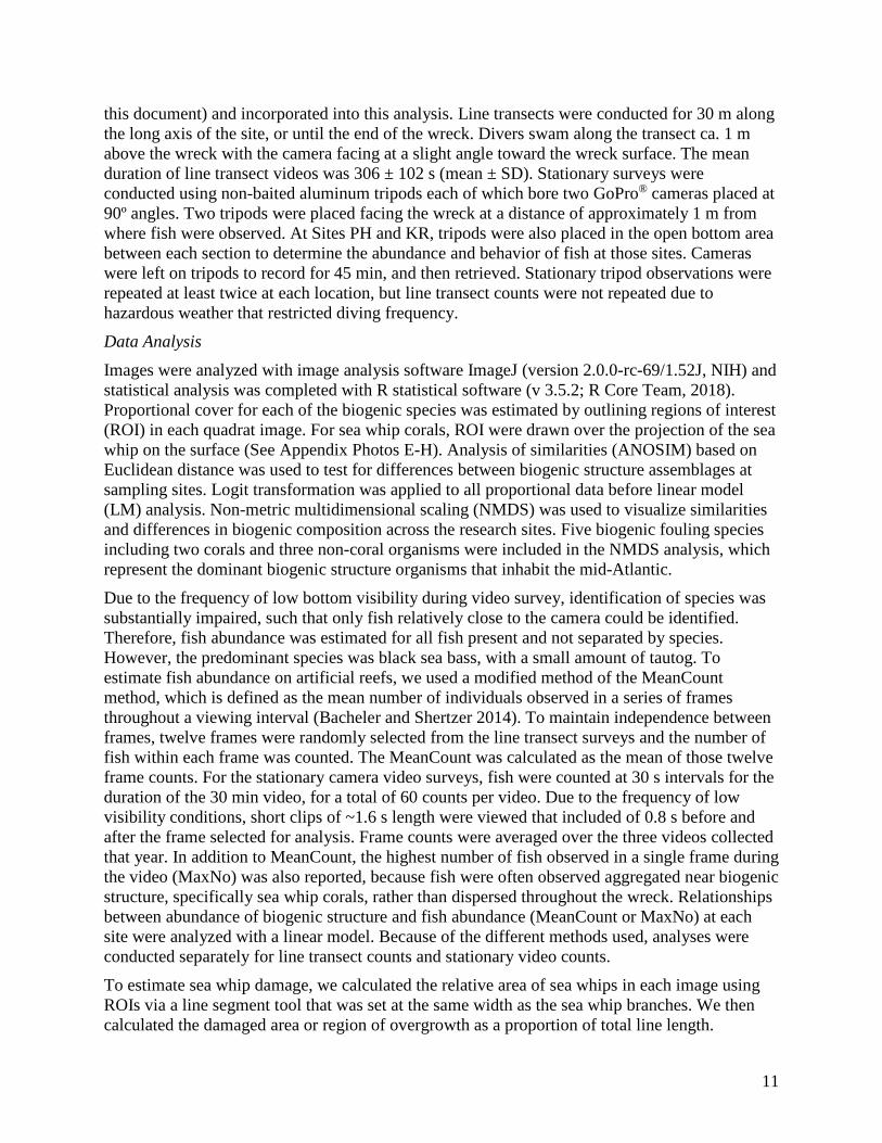
There have been few studies on habitats in the mid-Atlantic Bight by SCUBA or other in-situ methods due to unpredictable weather and turbid conditions. For these reasons, diving and data collection were restricted to the months of June through November during 2017 and 2018 and only conducted on days with a wave height ≤ 1 m. Fish abundance surveys were conducted June through August. If quadrat sampling could not be completed during the same sampling day, the site was resampled at a later time. During these months bottom water temperatures ranged from 9.31°C to 22.57°C and surface temperatures ranged from 13.48 to 27.23° C (CTD data). Bottom visibility in the mid-Atlantic is highly unpredictable and ranged from ~0.5 to ~18 m. Neither quadrat nor video data could be collected on days with bottom visibility < 1.5 m. Table 1.1. Sites surveyed during this study, including name, abbreviation, approximate age, depth, month in which fish abundance surveys were completed, and category, indicating whether sites were constructed deliberately or sank unintentionally. Site names are the common name of wreck for the region, however some site names are not universal.

Site Site Name Abbr. Approx. Age (y)

Approx. Depth (m)

Month Surveyed Category

1 Fenwick Shoals FW 120 10 July Unintentional 2 Elizabeth Palmer EP 104 23.5 July Unintentional 3 EP-2 E2 100 24 July Unintentional 4 Pharoby PH 37 20 June Deliberate 5 Blenny BL 30 23.5 July Deliberate 6 Kathleen Riggins RG 28 16.5 June Unintentional 7 Memorial Barge MM 26 18 — Deliberate 8 Sussex SX 24 24 July Deliberate 9 Navy Barge NV 19 20 July Deliberate 10 Barge BA 2 19 August Deliberate 11 New Hope NH 0.5 18 August Deliberate 12 Boiler Wreck BW NA 24 July Deliberate

Data Collection

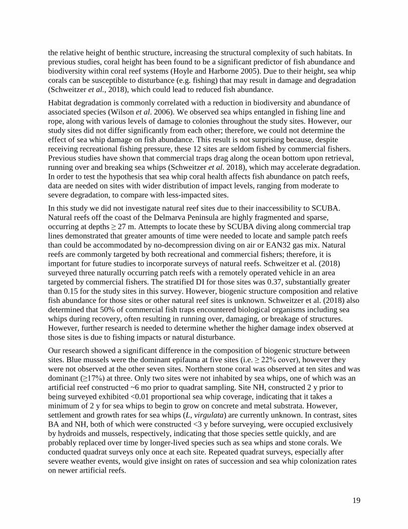
Quadrat sampling was used to estimate the proportional coverage of the dominant biogenic organisms: sea whip corals, putatively identified as Leptogorgia virgulata, northern stone coral, Astrangia poculata, blue mussels, Mytilus edulis, sponge, Cliona celata, and various hydroid species (e.g. Tubularia sp., Obelia sp., Campanularia sp.). Quadrat images (n = 11 to 60) were taken by SCUBA divers with a Canon DSLR camera in a housing attached to a 0.25 m2 PVC frame1. Images were taken at 1 m intervals along the long axis of the artificial reef for 30 m, or to end of the wreck. Quadrat sampling was conducted once at each of the sites. To assess sea whip damage, a haphazardly selected subset of sea whips was photographed with GoPro® Hero 4 action camera1 if abundant (e.g. > 1 m-2), otherwise all sea whips present were photographed.

1 Reference to trade names does not imply endorsement by either the University of Maryland Eastern Shore or funding sources.

10

Figure 1.1. Map of study sites showing the locations of the 12 artificial reefs off the coast of the Delmarva

(Delaware, Maryland, Virginia) peninsula.

Fish abundance on artificial reefs was estimated using two different types of underwater video survey: 1) line transect method, and 2) stationary cameras. Line transects were conducted at eight sites while stationary camera surveys were conducted at four of the sites. The latter method was used primarily to estimate fish abundance for an artificial reef construction project (Chapter 2 of

11

this document) and incorporated into this analysis. Line transects were conducted for 30 m along the long axis of the site, or until the end of the wreck. Divers swam along the transect ca. 1 m above the wreck with the camera facing at a slight angle toward the wreck surface. The mean duration of line transect videos was 306 ± 102 s (mean ± SD). Stationary surveys were conducted using non-baited aluminum tripods each of which bore two GoPro® cameras placed at 90º angles. Two tripods were placed facing the wreck at a distance of approximately 1 m from where fish were observed. At Sites PH and KR, tripods were also placed in the open bottom area between each section to determine the abundance and behavior of fish at those sites. Cameras were left on tripods to record for 45 min, and then retrieved. Stationary tripod observations were repeated at least twice at each location, but line transect counts were not repeated due to hazardous weather that restricted diving frequency.

Data Analysis

Images were analyzed with image analysis software ImageJ (version 2.0.0-rc-69/1.52J, NIH) and statistical analysis was completed with R statistical software (v 3.5.2; R Core Team, 2018). Proportional cover for each of the biogenic species was estimated by outlining regions of interest (ROI) in each quadrat image. For sea whip corals, ROI were drawn over the projection of the sea whip on the surface (See Appendix Photos E-H). Analysis of similarities (ANOSIM) based on Euclidean distance was used to test for differences between biogenic structure assemblages at sampling sites. Logit transformation was applied to all proportional data before linear model (LM) analysis. Non-metric multidimensional scaling (NMDS) was used to visualize similarities and differences in biogenic composition across the research sites. Five biogenic fouling species including two corals and three non-coral organisms were included in the NMDS analysis, which represent the dominant biogenic structure organisms that inhabit the mid-Atlantic.

Due to the frequency of low bottom visibility during video survey, identification of species was substantially impaired, such that only fish relatively close to the camera could be identified. Therefore, fish abundance was estimated for all fish present and not separated by species. However, the predominant species was black sea bass, with a small amount of tautog. To estimate fish abundance on artificial reefs, we used a modified method of the MeanCount method, which is defined as the mean number of individuals observed in a series of frames throughout a viewing interval (Bacheler and Shertzer 2014). To maintain independence between frames, twelve frames were randomly selected from the line transect surveys and the number of fish within each frame was counted. The MeanCount was calculated as the mean of those twelve frame counts. For the stationary camera video surveys, fish were counted at 30 s intervals for the duration of the 30 min video, for a total of 60 counts per video. Due to the frequency of low visibility conditions, short clips of ~1.6 s length were viewed that included of 0.8 s before and after the frame selected for analysis. Frame counts were averaged over the three videos collected that year. In addition to MeanCount, the highest number of fish observed in a single frame during the video (MaxNo) was also reported, because fish were often observed aggregated near biogenic structure, specifically sea whip corals, rather than dispersed throughout the wreck. Relationships between abundance of biogenic structure and fish abundance (MeanCount or MaxNo) at each site were analyzed with a linear model. Because of the different methods used, analyses were conducted separately for line transect counts and stationary video counts.

To estimate sea whip damage, we calculated the relative area of sea whips in each image using ROIs via a line segment tool that was set at the same width as the sea whip branches. We then calculated the damaged area or region of overgrowth as a proportion of total line length.

12

Proportional damage of individual sea whip corals was averaged at each site, and the mean value was used to assign a damage index (DI) from 1 to 5 (Table 2) as described in Schweitzer et al. (2018) (See Appendix Photos O, P). The proportional data was analyzed with a linear model to determine if sea whip DI differed between sites and if DI had an effect on fish abundance. Table 1.2. Criteria used to classify individual sea whip damage index (DI) and overall habitat DI for images captured. For individual sea whips, damage is defined as any visible tissue damage, exposed skeletal structure, or overgrowth by hydroids or bryozoans.

DI Damage Description 1 Minimal < 0.05 damage or overgrowth 2 Minor 0.06-0.25 damage or overgrowth 3 Moderate 0.26-0.50 damage or overgrowth 4 Severe 0.51-0.75 damage or overgrowth 5 Critical > 0.75 damage or overgrowth

Results Composition of artificial reefs

Data derived from quadrat images showed a significant difference between study sites, but with some overlap in biogenic assemblages (ANOSIM R = 0.32; p = 0.001; Fig. 1.2). The mean proportional coverage of biogenic structure on artificial reefs off the Delmarva coast was 0.47 ± 0.14. Proportional coverage was lowest at Site SX (0.27), and greatest at Site NV (0.81; Fig. 1.3). Sea whip corals (Leptogorgia sp.) and northern stone coral (A. poculata) were present on 10 of the 12 sites. One of the two sites void of sea whip corals was constructed 6 mo prior to the quadrat survey and only exhibited colonization by hydroid species (Site NH; Table 1.3). Blue mussels (M. edulis) were found on 5 of the 12 sites. Boring sponge (C. celata) was observed at 8 of the 12 sites. Site BW was the only location that contained all five structure-forming species. Results from the NMDS supported the results from the ANOSIM in that some sites exhibited distinctive biogenic structure communities, while others showed considerable overlap (Fig 2). Table 1.3. Proportional cover of biogenic structures by site. n is the number of quadrat images analyzed at each site; �̅�𝑥 is the mean proportional coverage for each variable: SW = sea whip coral, SC = northern stone coral, SP = boring sponge, MS = blue mussel, HY = hydroids.

Site n �̅�𝑥 SW �̅�𝑥 SC �̅�𝑥 SP �̅�𝑥 MS �̅�𝑥 HY FW 27 0.00 0.10 0.31 0.00 0.11 LP 36 0.06 0.17 0.05 0.00 0.15 E2 11 0.11 0.18 0.04 0.00 0.15 PH 60 0.14 0.11 0.10 0.00 0.07 BL 51 0.01 0.01 <0.01 0.23 0.24 RG 41 0.08 0.26 <0.01 0.00 0.00 MM 33 0.08 0.10 0.00 0.29 0.05 SX 31 0.17 0.07 <0.01 0.00 0.03 NV 37 0.11 <0.01 0.00 0.65 0.07 BA 27 <0.01 0.00 0.00 0.54 0.01 NH 31 0.00 0.00 0.00 0.00 0.35 BW 27 0.11 0.05 0.02 0.24 0.1

13

Northern stone coral and blue mussels were negatively correlated. Sites NV and NH were associated with blue mussel coverage, while sites EP, E2, PH, and RG were associated with northern stone coral (Fig. 1.2). Sea whip corals and hydroids were negatively correlated, suggesting a chronological succession of the fouling community. Sites PH, RG, MM, SX, NV, and BW were associated with sea whips, whereas sites BL and BA were associated with hydroids. Sites FW and PH were associated with boring sponge (Fig. 1.2).

Figure 1.2. Nonmetric multidimensional scaling analysis of biogenic structure assemblages at the 12 artificial reef sites off the Delmarva coast. P value is from the ANOSIM analysis. Variables: SW = sea whip corals; SC = northern stone coral; SP = boring sponge; MS = blue mussel; HY = hydroids. MeanCounts of fish were obtained from 11 of the 12 sites. Visibility was too poor for a video survey to be conducted at Site MM, and hazardous weather prevented additional outings. MeanCounts of fish were highest at Sites E2 and PH, and lowest at Sites FW and NH, whereas MaxNo was highest at Sites E2 and SX (Fig. 1.3, Table 1.4). No fish were observed swimming on open sandy bottom. MeanCounts and MaxNo were highly correlated (r2 = 0.94). A linear model using fish MeanCounts as the response variable and total proportional coverage as the predictor variable was not significant (ANOVA, F = 0.14; p = 0.72; r2 = 0.02), indicating that abundance of fish was not related to total proportional coverage of biogenic structure. MeanCounts were significantly related to proportional coverage of sea whip corals at sites with stationary tripods (p = 0.036; r2 = 0.48; Table 1.5; Fig. 1.5) as well as at sites where line transect video surveys were conducted (p = 0.014; r2 = 0.69).

14

Figure 1.3. Proportional cover of five structure-forming species at 12 study sites. Total = Cumulative total coverage of all five biogenic species groups from quadrat images. Table 1.4. Summary of fish MeanCount and MaxNo for underwater video census surveys.

Site MeanCount SD MaxNO FW 0.50 0.76 2 LP 5.25 2.18 14 E2 14.4 5.67 35 PH 7.49 3.07 24 BL 3.93 5.44 18 RG 5.05 2.66 18 MM –– –– –– SX 6.64 7.56 27 NV 4.36 4.86 15 NH 0.64 2.41 3 BA 1.57 0.84 7 BW 7.07 4.92 19

15

Table 1.5. ANOVA results from the linear model analysis for 11 of the 12 sites. Fish MeanCount is the response variable and biogenic structural species are the predictor variables.

Variable Sum Sq F value df P value Sea whips 73.87 9.31 10 0.028 Stone Coral 20.01 2.52 10 0.173 Sponge 0.13 0.17 10 0.904 Blue mussel 7.87 0.99 10 0.365 Hydroids 11.21 1.41 10 0.288

Evidence of habitat disturbance due to fishing (e.g. lures, fishing line, abandoned traps) was observed at 10 of the 12 sites (all but Sites E2 and BA). Observations of tangled fishing line were common at edges of shipwrecks. Fishing gear was observed in direct contact with sea whip corals at 9 of the 10 sites where sea whips occurred (Fig. 1.6). To determine if cumulative sea whip damage was related to reduced habitat quality and fish abundance we analyzed a total of 193 sea whip images from 10 of the 12 study sites, excluding Sites FW and NH, where sea whip corals were absent. Sea whips at most sites exhibited various levels of degradation (Fig. 1.7). However, despite evidence of fishing disturbance at all sites, with the exception of Site E2, the mean damage index (DI) was 0.15 ± 0.19 SD for all sites, which is indicative of minor levels of degradation (Table 1.6). Site LP showed the highest DI with a mean of 0.26 ± 0.19 indicating a moderate level of degradation, however this was not significantly different from the other sites (p = 0.061). Table 1.6. Summary of the mean proportional damage for sea whips and the habitat DI by site. n is the number of sea whips analyzed at each site. �̅�𝑥 is the mean proportional damage for the measured sea whips. SD is the standard deviation. Max is the highest proportional damage observed. Min is the lowest proportional damage observed. D.I. is the damage index assigned to the site.

Site n 𝒙𝒙� SD Max Min D.I. Degradation Category

1 0 – – – – – – 2 31 0.26 0.19 0.77 0.05 3 Moderate 3 11 0.02 0.02 0.02 0.00 1 Minimal 4 19 0.15 0.24 1.00 0.00 2 Minor 5 17 0.15 0.24 1.00 0.00 2 Minor 6 19 0.07 0.05 0.18 0.02 2 Minor 7 24 0.15 0.15 0.47 0.00 2 Minor 8 21 0.12 0.11 0.40 0.00 2 Minor 9 26 0.11 0.15 0.66 0.00 2 Minor 10 7 0.15 0.30 0.82 0.00 2 Minor 11 0 – – – – – – 12 28 0.15 0.21 0.78 0.00 2 Minor

16

Figure 1.4. Photos illustrating fish and sea whip density at two locations (Sites SX and NV). A) Region of Site SX with minimal biostructure. White arrow highlights the single fish located within this frame. B) Region of Site SX with higher sea whip coverage, on same dive as 4A. White arrows show the location of the 14 fish observed. C) An area of Site NV that is mostly composed of rock, broken shells and concrete blocks with a single sea whip coral and some colonies of northern stone coral on the wall of the wreck. White arrows show the locations of four fish. D) Region of Site NV with increased sea whip coverage during same dive as 4C. White arrows show the location of 12 fish.

Discussion The presence of autogenic engineers often increases habitat quality resulting in increases in species abundance and biodiversity across terrestrial, freshwater, and marine ecosystems (Jones et al. 1994; Hastings et al. 2007). However, not all types of structures are equivalent, or have positive correlations with species biodiversity and abundance (Jones et al. 1997). Therefore, it is important to understand the relationships between composition of biogenic structure and its effect on community structure. The mid-Atlantic Bight is a poorly studied region inhabited by multiple economically important species (Hostetter and Munroe 1993; Shepherd et al. 2002) that are exploited both recreationally and commercially. Many of these species (e.g. black sea bass and tautog) are considered structure oriented, but it remains unclear if biogenic structure affects their habitat selection. Insights into the relationships between biogenic structure and fish abundance will be useful for developing ecosystem-based fisheries management (EBFM).

17

Figure 1.5. Relationship of MeanCount and proportional sea whip coverage for 11 of the 12 study sites. There is a significant positive correlation (p = 0.018; r2 = 0.48).

Figure 1.6. Two photographs showing representative examples of anthropogenic disturbance observed at the research sites. A) Sea whip coral from Site PH entangled in rope. B) Sea whip from Site NV with fish line entangled around a portion of branches.

18

Figure 1.7. Photographs showing sea whip corals with four different degrees of damage. A) Sea whip coral exhibiting a minimal proportional damage index of 0.02. White arrow highlights the region of damage. B) Sea whip coral exhibiting minor proportional damage index of 0.13, localized at the base of the coral. C) Sea whip coral exhibiting a severe proportional damage index of 0.51. The white arrow is showing a region where the tissue has completely decayed, exposing the skeletal structure. This coral also exhibits colonization by hydroids. D) Sea whip coral exhibiting critical proportional damage index of 1.00 with no live tissue remaining. In this study we measured habitat composition and relative abundance of fish on 12 artificial reef sites to determine if relationships existed between biogenic structure and habitat use by fish. We concluded that abundance of fish was significantly correlated with abundance of sea whip coral and that fish were often aggregated near sea whips. In fact, sites without sea whips, or having a proportional abundance <0.01, exhibited low values for both fish MeanCounts and MaxNo. Within the mid-Atlantic Bight, sea whip corals are the primary autogenic engineer that increases

19

the relative height of benthic structure, increasing the structural complexity of such habitats. In previous studies, coral height has been found to be a significant predictor of fish abundance and biodiversity within coral reef systems (Hoyle and Harborne 2005). Due to their height, sea whip corals can be susceptible to disturbance (e.g. fishing) that may result in damage and degradation (Schweitzer et al., 2018), which could lead to reduced fish abundance.

Habitat degradation is commonly correlated with a reduction in biodiversity and abundance of associated species (Wilson et al. 2006). We observed sea whips entangled in fishing line and rope, along with various levels of damage to colonies throughout the study sites. However, our study sites did not differ significantly from each other; therefore, we could not determine the effect of sea whip damage on fish abundance. This result is not surprising because, despite receiving recreational fishing pressure, these 12 sites are seldom fished by commercial fishers. Previous studies have shown that commercial traps drag along the ocean bottom upon retrieval, running over and breaking sea whips (Schweitzer et al. 2018), which may accelerate degradation. In order to test the hypothesis that sea whip coral health affects fish abundance on patch reefs, data are needed on sites with wider distribution of impact levels, ranging from moderate to severe degradation, to compare with less-impacted sites.

In this study we did not investigate natural reef sites due to their inaccessibility to SCUBA. Natural reefs off the coast of the Delmarva Peninsula are highly fragmented and sparse, occurring at depths ≥ 27 m. Attempts to locate these by SCUBA diving along commercial trap lines demonstrated that greater amounts of time were needed to locate and sample patch reefs than could be accommodated by no-decompression diving on air or EAN32 gas mix. Natural reefs are commonly targeted by both recreational and commercial fishers; therefore, it is important for future studies to incorporate surveys of natural reefs. Schweitzer et al. (2018) surveyed three naturally occurring patch reefs with a remotely operated vehicle in an area targeted by commercial fishers. The stratified DI for those sites was 0.37, substantially greater than 0.15 for the study sites in this survey. However, biogenic structure composition and relative fish abundance for those sites or other natural reef sites is unknown. Schweitzer et al. (2018) also determined that 50% of commercial fish traps encountered biological organisms including sea whips during recovery, often resulting in running over, damaging, or breakage of structures. However, further research is needed to determine whether the higher damage index observed at those sites is due to fishing impacts or natural disturbance.

Our research showed a significant difference in the composition of biogenic structure between sites. Blue mussels were the dominant epifauna at five sites (i.e. ≥ 22% cover), however they were not observed at the other seven sites. Northern stone coral was observed at ten sites and was dominant (≥17%) at three. Only two sites were not inhabited by sea whips, one of which was an artificial reef constructed ~6 mo prior to quadrat sampling. Site NH, constructed 2 y prior to being surveyed exhibited <0.01 proportional sea whip coverage, indicating that it takes a minimum of 2 y for sea whips to begin to grow on concrete and metal substrata. However, settlement and growth rates for sea whips (L, virgulata) are currently unknown. In contrast, sites BA and NH, both of which were constructed <3 y before surveying, were occupied exclusively by hydroids and mussels, respectively, indicating that those species settle quickly, and are probably replaced over time by longer-lived species such as sea whips and stone corals. We conducted quadrat surveys only once at each site. Repeated quadrat surveys, especially after severe weather events, would give insight on rates of succession and sea whip colonization rates on newer artificial reefs.

20

Fish abundance was estimated via two underwater video survey methods: line transects and non-baited stationary cameras, conducted over the course of two years, which is a limitation to this study. Ideally, abundance censuses would be conducted in a synoptic fashion; however, weather and water conditions in the mid-Atlantic Bight are unpredictable, and were often deemed too hazardous for SCUBA surveys, making it difficult to collect data within specific time blocks. The video surveys acquired from the stationary cameras at four sites (Sites LP, E2, PH, & RG) could result in an upward bias of the MeanCount; nevertheless, fish MeanCount still showed a significant correlation with sea whip abundance at the remaining seven sites. Additional surveys are needed to understand how fish abundance at sites can vary throughout and over years since many of the prominent fish species (e.g. black sea bass and tautog) are seasonal migrators.

Our study is the first to quantify the composition of biogenic structure on artificial reefs off the coast of Delmarva Peninsula and to show that fish abundance is significantly correlated with the presence and abundance of sea whip corals. Construction of artificial reefs off the coast of Delmarva occurs on an annual basis to increase the local abundance of economically valuable species. Creating artificial reefs near regions with established sea whip coral populations may help facilitate sea whip settlement and colonization of new structures. Future studies to determine variations in fish abundance over time, and to determine the succession of biogenic structure would be useful. In addition, future surveys of naturally occurring patch reefs should be conducted, in order to gain a more detailed assessment of habitat quality in the mesophotic regions of the Mid-Atlantic Bight.

References Bacheler, N.M. and Shertzer, K.W. (2014) Estimating relative abundance and species richness

from video surveys of reef fishes. Fishery Bulletin 113, 15–26.

Bohnsack, J.A. (1989) Are high densities of fishes at artificial reefs the result of habitat limitation or behavioral preference? Bulletin of Marine Science 44, 631–645.

Cheminee, A., Merigot, B., Vanderklift, M. and Francour, P. (2016) Does habitat complexity influence fish recruitment? Mediterranean Marine Science 17, 39–46.

Daleo P, Escapa M, Alberti J, Iribarne O. (2004) Negative effects of an autogenic ecosystem engineer: interactions between coralline turf and an ephemeral green alga. Mar Ecol Prog Ser 315: 67 – 73.

Diaz, R., Solan, M., Valente, R. (2004) A review of approaches for classifying benthic habitats and evaluating habitat quality. Journal of Environmental Management 73, 165–181.

Downs, C. A., Woodley, C. M., Richmond, R. H., Lanning, L. L., Owen, R. (2005). Shifting the paradigm of coral-reef ‘health’assessment. Marine Pollution Bulletin, 51(5-7), 486-494.

Dudgeon, S.R., Aronson, R.B., Bruno, J.F. and Precht, W.F. (2010) Phase shifts and stable states on coral reefs. Marine Ecology Progress Series 413, 201–216.

Fabrizio, M. C., Manderson, J. P., Pessutti, J. P. (2013). Habitat associations and dispersal of black sea bass from a mid-Atlantic Bight reef. Marine Ecology Progress Series, 482, 241-253.

21

Feigenbaum, D., Bushing, M., Woodward, J. and Friedlander, A. (1989) Artificial reefs in Chesapeake Bay and nearby coastal waters. Bulletin of Marine Science 44, 734–742.

Forrester, G.E. and Steele, M.A. (2004) Predators, Prey Refuges, And The Spatial Scaling Of Density-Dependent Prey Mortality. Ecology 85, 1332–1342.

Fox, J., Weisberg, S., Adler, D., Bates, D., Baud-Bovy, G., Ellison, S., ... & Heiberger, R. (2012). Package ‘car’. Vienna: R Foundation for Statistical Computing.

Garpe, K.C. and Öhman, M.C. (2003) Coral and fish distribution patterns in Mafia Island Marine Park, Tanzania: fish–habitat interactions. Hydrobiologia 498, 191–211.

Gibson, R.N. (1994) Impact of habitat quality and quantity on the recruitment of juvenile flatfishes. Netherlands Journal of Sea Research 32, 191–206.

Gotelli, N.J. (1991) Demographic models for Leptogorgia virgulata, a shallow‐water gorgonian. Ecology 72, 457–467.

Granneman, J.E. and Steele, M.A. (2015) Effects of reef attributes on fish assemblage similarity between artificial and natural reefs. ICES Journal of Marine Science 72, 2385–2397.

Gregor, C. and Anderson, T. (2016) Relative importance of habitat attributes to predation risk in a temperate reef fish. Environmental Biology of Fishes.

Grossman, G., Jones, G. and Seaman, W. (1997) Do Artificial Reefs Increase Regional Fish Production? A Review of Existing Data. Fisheries 22, 17–23.

Harborne, A., Mumby, P. and Ferrari, R. (2012) The effectiveness of different meso-scale rugosity metrics for predicting intra-habitat variation in coral-reef fish assemblages. Environmental Biology of Fishes 94, 431–442.

Hastings, A. et al. (2007). Ecosystem engineering in space and time. Ecology letters, 10(2), 153-164.

Hixon, M.A. and Beets, J.P. (1993) Predation, Prey Refuges, and the Structure of Coral‐Reef Fish Assemblages. Ecological Monographs 63, 77–101.

Hostetter, E.B. and Munroe, T.A. (1993) Age, growth, and reproduction of tautog Tautoga onitis (Labridae: Perciformes) from coastal waters of Virginia. Fishery Bulletin 91, 45–64.

Hughes, T. P., Graham, N. A., Jackson, J. B., Mumby, P. J., Steneck, R. S. (2010). Rising to the challenge of sustaining coral reef resilience. Trends in ecology & evolution, 25(11), 633-642.

Johnson, D.W. (2007) Habitat complexity modifies post‐settlement mortality and recruitment dynamics of a marine fish. Ecology 88, 1716–1725.

Jones, C. G., Lawton, J. H., & Shachak, M. (1994). Organisms as ecosystem engineers. In Ecosystem management (pp. 130-147). Springer, New York, NY.

Jones, C. G., Lawton, J. H., & Shachak, M. (1997). Positive and negative effects of organisms as physical ecosystem engineers. Ecology, 78(7), 1946-1957.

Jones, G.P., McCormick, M.I., Srinivasan, M. and Eagle, J.V. (2004) Coral decline threatens fish biodiversity in marine reserves. Proceedings of the National Academy of Sciences of the United States of America 101, 8251–3.

22

Komyakova, V., Jones, G. and Munday, P. (2018) Strong effects of coral species on the diversity and structure of reef fish communities: A multi-scale analysis. PLOS ONE 13, e0202206.

Lê, S., Josse, J., & Husson, F. (2008). FactoMineR: an R package for multivariate analysis. Journal of statistical software, 25(1), 1-18.

Lenth, R. V. (2016). Least-squares means: the R package lsmeans. Journal of statistical software, 69(1), 1-33.

Lotze, H., Lenihan, H., Bourque, B., et al. (2006) Depletion, Degradation, and Recovery Potential of Estuaries and Coastal Seas. Science 312, 1806–1809.

McCauley, D.J., Pinsky, M.L., Palumbi, S.R., Estes, J.A., Joyce, F.H. and Warner, R.R. (2015) Marine defaunation: animal loss in the global ocean. Science 347, 1255641.

Miller, R., Hocevar, J., Stone, R. and Fedorov, D. (2012) Structure-Forming Corals and Sponges and Their Use as Fish Habitat in Bering Sea Submarine Canyons. PLoS ONE 7, e33885.

Newman, M. J., Paredes, G. A., Sala, E., Jackson, J. B. (2006). Structure of Caribbean coral reef communities across a large gradient of fish biomass. Ecology letters, 9(11), 1216-1227.

Oksanen, J., et al. (2010). vegan: Community Ecology Package. R package version 1.17-2. http://cran. r-project. org>. Acesso em, 23, 2010.

Richmond, R.H., (1996). Coral reef health: concerns, approaches and needs. In: Crosby, M.P., Gibson, G.R., Potts, K.W. (Eds.), A

Coral Reef Symposium on Practical, Reliable. Low Cost Monitoring Methods for Assessing the Biota and Habitat Conditions of

Coral Reefs, January 26–27, 1995. Office of Ocean and Coastal

Resource Management, NOAA, Silver Spring, MD, pp. 25–30.

R Core Team (2018). R: A language and environment for statistical computing. R Foundation for Statistical Computing, Vienna, Austria. URL https://www.R-project.org/.

Robertson, D.R. and Sheldon, J. (1979) Competitive interactions and the availability of sleeping sites for a diurnal coral reef fish. Journal of Experimental Marine Biology and Ecology 40, 285–298.

Scharf, F.S., Manderson, J.P. and Fabrizio, M.C. (2006) The effects of seafloor habitat complexity on survival of juvenile fishes: species-specific interactions with structural refuge. Journal of Experimental Marine Biology and Ecology 335, 167–176.

Schweitzer, C. C., and B. G. Stevens. in review. The importance of soft coral sea whips (Leptogorgia sp.) to fish abundance on artificial reefs in the Mid-Atlantic Bight. PeerJ.

Schweitzer, C.C., Lipcius, R.N. and Stevens, B.G. (2018) Impacts of a multi-trap line on benthic habitat containing emergent epifauna within the Mid-Atlantic Bight. ICES Journal of Marine Science.

Scott, M.E., Smith, J.A., Lowry, M.B., Taylor, M.D. and Suthers, L.M. (2015) The influence of an offshore artificial reef on the abundance of fish in the surrounding pelagic environment. Marine and Freshwater Research 66, 429–437.

23

Seemann, J., Yingst, A., Stuart-Smith, R., Edgar, G. and Altieri, A. (2018) The importance of sponges and mangroves in supporting fish communities on degraded coral reefs in Caribbean Panama. PeerJ 6, e4455.

Shepherd, G. R., Moore, C. W., & Seagraves, R. J. (2002). The effect of escape vents on the capture of black sea bass, Centropristis striata, in fish traps. Fisheries research, 54(2), 195-207.

Sherman, R., Gilliam, D. and Spieler, R. (2002) Artificial Reef Design: Void Space, Complexity, and Attractants. ICES Journal of Marine Science 59, S196–S200.

Smith, J.A., Cornwell, W.K., Lowry, M.B. and Suthers, I.M. (2017) Modelling the distribution of fish around an artificial reef. Marine and Freshwater Research.

Soler-Hurtado, M., Megina, C. and López-González, P. (2018) Structure of gorgonian epifaunal communities in Ecuador (eastern Pacific). Coral Reefs 37, 723–736.

Thrush, S.F., Halliday, J., Hewitt, J.E. and Lohrer, A.M. (2008) The effects of habitat loss, fragmentation, and community homogenization on resilience in estuaries. Ecological Society of America 18, 12–21.

Wilson, S. K., Graham, N. A., Pratchett, M. S., Jones, G. P., & Polunin, N. V. (2006). Multiple disturbances and the global degradation of coral reefs: are reef fishes at risk or resilient?. Global Change Biology, 12(11), 2220-2234.

24

25

Chapter 2. Effects of Habitat Enhancement on Local Fish Abundance: A Before-After/Control-Impact (BACI) Design Study on Artificial reefs in the Mid-Atlantic Bight Cara C. Schweitzer and Bradley G. Stevens

Adapted from: Schweitzer, C.C. and B. G. Stevens (MS in preparation). Response of fish abundance to increased seascape connectivity using a mosaic corridor connecting artificial reefs in the Mid-Atlantic Bight.

Abstract Seascape connectivity, the arrangement and proximity of nearby habitats, which can facilitate or impede animal movements, has been a well-studied research topic in terrestrial systems and is becoming a topic of interest in marine systems. Despite this, there are few studies that actively increase seascape connectivity to existing reefs. To determine if increasing seascape connectivity increases fish abundance on habitat patches, we constructed a stepping-stone corridor connecting two established sections of an artificial reef based on a Before-After-Control-Impact (BACI) experimental design. Fish abundance was estimated by conducting stationary video surveys during three sampling seasons for one year before corridor placement (the impact) and one year after impact at the study site and control site. We observed a significant increase in fish abundance at the corridor (impact) site and no significant change at the control site. Furthermore, fish were observed on the corridor during all three sampling series. This study tests the terrestrial concept of corridor functional connectivity of patches to facilitate animal movement and abundance. This small-scale study demonstrates that increasing corridor connectivity may be an effective method for enhancing habitats in marine as well as terrestrial ecosystems.

Introduction Landscape connectivity of terrestrial systems and the effect of increasing and decreasing connectivity have been well studied over the decades (Fahrig and Merriam 1985; Fahrig 2001; Fahrig 2002; Kindlmann and Burel 2008; Ayram et al. 2016). Within terrestrial ecosystems enhancing landscape connectivity has been shown to increase species abundance, biodiversity, and viability (Schooley and Branch 2011; Ayram et al. 2016). A popular mechanism for increasing habitat patch connectivity is the implementation of corridors (Beier and Noss 1998; Bennett 2003; Hilty 2012). Although there has been some debate on the success rate of corridors, some studies show that corridors help facilitate the movement of birds, insects, reptiles, and mammals, and have also been shown to increase plant richness (Beier and Noss 1998; Schooley and Branch 2011). In marine ecosystems, seascape connectivity has only more recently been studied. However, there have been few experimental studies that have investigated the effects of connectivity through manipulation of artificial reefs or corridor construction.

Within marine ecosystems, increasing seascape connectivity results in positive effects on marine reserve performance, accelerated recovery of community composition after disturbance, and increased facilitation of fish movement (Mumby and Hastings 2008; McCook et al. 2009; Olds et al. 2012; Engelhard et al. 2017). These studies, however, did not manipulate connectivity through artificial reef construction. There are few studies of the effects of patch connectivity on fish aggregation and abundance on those sites.

26

Within the mid-Atlantic Bight, benthic structure is predominantly provided by artificial reefs, which are frequently constructed, often in isolation. Isolated reefs exhibit slower settlement rates of spores and larvae (Svane and Petersen 2001; Connell and Slatyer 1977) and reduced fish settlement (Overholtzer-McLeod 2006; Turgeon et al. 2010) compared to artificial reefs constructed in closer proximity to other reef systems. As shown in Chapter 1, abundance of fish on Delmarva reefs was significantly associated with relative abundance of sea whip corals, and recently constructed artificial reefs exhibited lower relative coral and fish abundance compared to established artificial reefs (Chapter 1, Schweitzer and Stevens in review).

In this study we explore the terrestrial corridor model by increasing seascape connectivity between two sections of established artificial reefs. We use a Before-After-Control-Impact (BACI; Smith 2014) experimental design to statistically assess whether a mosaic stepping-stone style corridor connecting two established sections of an artificial reef increases fish abundance at that site compared to a control site.

Methods We used a simple two year before-after-control-impact (BACI) design to measure the change in fish abundance after increasing connectivity between an established artificial reef. Two artificial sites (PH and RG in Table 1.1) located ~ 14.5 km off the coast of Maryland, USA were selected based on SCUBA accessibility and spatial pattern. Both sites had broken into two distinct sections of established structure, separated by open sandy bottom. The control site (RG in Table 1.1) is designated as Site C, or CS for the two structured portions. It is a natural shipwreck that sank accidentally in 1991 and is still largely intact; its two sections are separated by ~24 m and lie at a depth of 16.7 m. The impact site (Site PH in Table 1.1), designated as site I (or IS for the structured portions) was a wooden vessel sunk intentionally in 1980; its two sections are separated by ~120 m at a depth of 19.8 m. The open bottom areas between the structured sections at sites C and I were designated CO and IO, respectively. Sites C and I are separated by a distance of 1.3 km, and both sites are subject to recreational fishing pressure. Site C is primarily colonized with sea whip Leptogorgia virgulata and northern stone corals Astrangia poculata. In addition to sea whip and northern stone corals, Site I is colonized by the boring sponge Cliona celata, and various hydroid species (i.e. Tubularia sp., Obelia sp., Campanularia sp; see Chapter 1 for detailed descriptions of the sites and biogenic structure).

At the impact site, a mosaic stepping-stone style corridor was constructed on the open bottom between the two structured sections. The corridor was constructed with concrete oyster castles stacked to form pyramid-like structures of various heights (See Appendix Photos K, L). Three size categories of pyramids were placed: large = 4 tiers; medium = 3 tiers; small = 2 tiers (Table 2.1). A total of 29 pyramids were deployed via a utility vessel December 21, 2016 (Fig. 2.1), spaced at intervals of ca. 6 m. Construction occurred during winter because most fish had undergone a seasonal migration to deeper offshore waters at that time. Site C did not receive any pyramids or other modifications. Table 2.1. Specifications of the pyramids that comprise the stepping stone corridor. Tier refers to the layers of oyster castle blocks in each pyramid. n Blocks are the number of blocks used to build each pyramid size. n pyramids are the number of pyramids of each tier size.

Tier n Blocks n Pyramids 2 5 15 3 14 14 4 30 4

27

To estimate fish abundance at the research sites, two GoPro® cameras were fastened on non-baited aluminum tripods and set facing outward at 90º angles (See Appendix Photos A, B, I). Cameras were set to record at a rate of 60 frames s-1 and at a resolution of 1080 x 720 pixels, with an approximate field of view of 90º. Tripods were placed by divers approximately 1 m from each structure (CS or IS) in areas where fish were observed. Tripods were also placed in the stretch of open bottom between the separated sections of both the study sites (CO and IO), at a distance of ~10.5 m and ~18 m away from the structure for Sites C and I, respectively. Cameras were left to record for 45 to 50 min in order to obtain at least 30 min of video that was void of diver interruptions. Tripods were then retrieved and placed on the second structured section of

A B C

Figure 2.1. Pyramids made of oyster-castle blocks that were used to create the corridor. A) Image of 3-tier and 4-tier pyramids. B) A 4-tier pyramid with white arrows highlighting fish. C) A 3-tier pyramid that landed upside down.

28

the wreck. Both sections of a site were recorded within a single sampling day. Video surveys were conducted approximately six months before (B) augmentation (2016), and 6–8 months after (A) augmentation (2017). Video surveys were conducted during three time periods in each year: early summer, mid-summer, and fall. Weather in the mid-Atlantic Bight is highly variable, unpredictable, and causes frequent turbid conditions, which can impede scuba accessibility and video surveys due to poor visibility. Bottom visibility < 1.5 m was deemed too poor for video surveys. Due to weather restrictions, our sampling series occurred during 2-week windows with a minimum of 4 weeks between each survey (Table 2.2). Table 2.2. Dates of video surveys at the research sites before and after corridor implementation. Video and data analysis were conducted using Final Cut Pro X© 10.4 (Apple Inc., Cupertino, California USA) and GraphPad Prism Software 7.0c (GraphPad Software Inc., La Jolla California USA). Videos were trimmed to 31 min and edited with color corrections to enhance the clarity of the video. Fish abundance was estimated using a modification of the MeanCount method described in Bacheler and Shertzer (2014). Fish were counted at 30 s intervals for the duration of the 30 min video, for a total of 60 counts per video. Due to the frequency of low visibility conditions, counting fish in still frames was unreliable, therefore short clips of ~1.6 s length were viewed that included of 0.8 s before and after the frame selected for analysis. Fish movement within that interval permitted a more precise count. The total number of fish observed during the clip was recorded for the count. Furthermore, low visibility conditions substantially impaired species identification, such that only fish relatively close to the camera could be identified. Therefore, fish abundance was counted in aggregate, and not separated by species. Values of fish abundance are expressed as mean fish-per-frame (fpf) ± standard error (SE)

We used a BACI design to analyze the video count data, in which surveys were designated as belonging to Before (2016) or After (2017) groups at each of the sections of the control and impact site. Linear mixed effects modeling (LME) was used to determine the effects of various factors. Multiple models were tested that included different factors: Time (i.e. Before vs. After), Site (C vs I), Sub-sites (CS, CO, IS, IO), and the interaction between Time and Site. Since multiple cameras were used to determine fish counts, videos analyzed during a sampling series were treated as pseudo-replicates. In all models, the two cameras on each tripod were treated as random effects. A null model containing only the intercept was also tested. The Akaike Information Criterion (AIC) was used to select the best fit model. The Δi values were used to rank the different models (mi) against the null model. Additionally, a multiple-comparisons 2-way ANOVA was conducted to look at annual changes of fish abundance between sites. We corrected for multiple comparisons with the Bonferroni correction and report the adjusted p values. The BACI interaction effect estimate (differential change) was calculated using the equation: 𝐵𝐵𝐵𝐵𝐵𝐵𝐵𝐵� = μCA − μCB − (μIA −μIB).

Before After Site Series 1 Series 2 Series 3 Series 1 Series 2 Series 3 Control 06/15/16 9/09/16 10/30/16 7/19/17 9/16/17 11/12/17 Impact 06/16/16 9/18/16 10/19/16 7/11/17 9/04/17 11/12/17

29

Results Despite our best efforts, some of the pyramids landed upside down, and others fell apart during winter storms. To estimate fish abundance on the research sites, six recordings were attempted with a goal of 360 frame counts for each site per sampling series: four recordings of the artificial reef sections and two recordings of the open bottom separating the sections. However, due to poor weather conditions, poor visibility, and strong currents knocking over tripods, the goal of 360 frame counts was met only once (Table 2.3). Fish were observed on pyramids at Site I during all three series, and schools of fish were observed swimming between pyramids (Fig. 2.1). Table 2.3. Mean of fish counts during three sampling series in two years for the Control and Impact sites. Control (CS) = established structure at the control site; Control (CO) = open sand between the two structures at the control site; Impact (IS) = established structure at the impact site; Impact (IO) = open sand between the structure (Before) and site of corridor construction (After). All values displayed as mean fish-per-frame (fpf) from all survey videos, plus/minus standard error (�̅�𝑥 ± SE).

Time Site Section Code Series 1 Series 2 Series 3 Annual Before Control Structured CS 7.17 ± 0.24 1.23 ± 0.10 7.06 ± 0.29 5.15 ± 0.19 Open CO 0.00 ± 0.00 0.00 ± 0.00 0.00 ± 0.00 0.00 ± 0.00 Impact Structured IS 8.53 ± 0.27 11.75 ± 0.39 3.55 ± 0.30 8.23 ± 0.24 Open IO 0.00 ± 0.00 0.00 ± 0.00 0.00 ± 0.00 0.00 ± 0.00 After Control Structured CS 7.68 ± 0.29 1.07 ± 0.13 5.82 ± 0.56 5.61 ± 0.27 Open CO 0.02 ± 0.02 0.00 ± 0.00 0.00 ± 0.00 0.01 ± 0.01 Impact Structured IS 6.23 ± 0.28 13.93 ± 0.71 5.24 ± 0.25 8.14 ± 0.30 Open IO 6.55 ± 0.28 4.78 ± 0.16 8.50 ± 0.27 6.35 ± 0.34

Fish abundance at site C was higher on the structured portions (mean >5.0 fpf) than on the open bottom (CO; mean 0.0 fpf), but differed little between years (t test; p = 0.82; Fig. 2.2). Only one fish was observed on the open sand in 2017. Abundance varied seasonally, with abundance during survey series 2 being lower than either series 1 or 3, and this pattern was similar in both years (F = 6.4; p = 0.12).

Fish abundance at site I in 2016 was also higher on the structured portions (mean ~ 8.2 fpf) than on the open bottom (mean 0.0 fpf, Fig. 2.3). However, in 2017, after corridor construction, mean abundance on the structured portions was similar to 2016, but the mean on open bottom increased significantly to ~6.4 fpf (t test, p = 0.001). Abundance at site I also varied seasonally, but in the opposite direction from site C, with abundance during survey series 2 being significantly greater (p < 0.001), than either series 1 or 3, which did not differ (p = 0.29), and this pattern was similar in both years (F = 6.4; p = 0.12).

When averaged across all series, fish abundance increased only at the impacted, open bottom portion of site I, and there were no changes at the structured portions of either site, or at the non-impacted open-bottom portion of site C (Fig. 2.4). The BACI interaction effect estimate was: 𝐵𝐵𝐵𝐵𝐵𝐵𝐵𝐵� = 2.98 ± 0.27 (Fig. 2.4). The best mixed effects model was model m5, which included Time, Series, Subsites, and Time x Site interactions (Table 2.4). Therefore we concluded that the increase in observed fish abundance was due to the corridor implementation.

30

Figure 2.2. Fish abundance at the Control site. C = established structure; CO = open sand between the control sections. Horizontal bars are the annual means of fish counts before and after the corridor construction (Table 2.3).

Figure 2.3. Fish abundance at the Impact site. I = established structure; IO = open sand before impact; corridor after placement. Horizontal bars are the annual means of fish counts before and after the corridor construction (Table 2.3).

31

Figure 2.4. Annual mean fish abundance observed at structured and open portions of each site. C = established structure at the Control site; CO = open sand between the structure sections; I = established structure at the Impact site; IO = the modified section of the Impact site. Table 2.4. Comparisons of mixed effects models m0 – m5, where m0 is the null model; all models included cameras as a random effect. Time = before (2016) vs after (2017) corridor construction; Series = three sampling series of early summer, mid-summer, and fall; Site = control vs impact sites as two categories (including structured/unstructured subsites); TxS = interaction of Site (control/impact) and Time (before/after); Subsites = control and impact site separated into established structure and open space; TxSS = interaction of Time and Subsites; df = degrees of freedom; Loglik = log likelihood; AIC = Akaike information criterion value; ΔI = increase in AIC value from the selected model (bolded); wi = model probability. Model m5 was selected as the best fit model.

Model Variables df Loglik AIC Δi wi m5 Time, TxS, Series, Subsites 12 -6966.43 13957.0 — 0.992 m4 Time, TxS, Subsites 10 -6973.24 13966.6 9.58 0.008 m3 Time, Site, Series, TxS 8 -7156.83 14329.7 372.72 0.000 m2 Time, Site, TxSS 6 -7193.89 14399.8 442.83 0.000 m1 Time 4 -7258.38 14524.8 567.79 0.000 m0 Intercept only 3 -7287.24 14580.5 623.50 0.000

Discussion This study tested a common terrestrial method to increase seascape connectivity in an attempt to increase fish abundance on an artificial reef off the coast of Ocean City, Maryland. Connectivity was increased by constructing a stepping stone style corridor connecting two established patches of an artificial reef. This experimental design was based on the Before-After-Control-Impact (BACI) designs (Smith 2014).

32

Our results showed that fish abundance increased significantly on the corridor within a few months of construction, but did not change at the unmodified portions of either site. After corridor implementation, the impact site showed a significant increase in fish abundance not only from the previous year, but also when compared to the control site. Fish abundance recorded on the established sections did not change significantly between years at either site indicating that the observed increase in fish abundance was a result of the corridor implementation. We also observed a significant change in abundance between sampling series at both sites, which occurred both before and after the corridor. Interestingly, the seasonal variation at each site was identical between years, but exhibited opposite patterns between sites, and persisted after corridor construction. During both 2016 and 2017, the control site showed a reduced abundance during Series 2 before increasing to numbers similar to what was observed during Series 1. At the impact site during both 2016 and 2017, fish abundance increased in Series 2 and then decreased in Series 3. However, after corridor implementation the reduction in fish abundance during Series 3 was not as pronounced.

These results demonstrate that corridor connectivity can be an effective method to increase fish abundance on isolated habitat patches. Our observations support previous research that investigated relationships in seascape connectivity. Turgeon et al. (2010) showed evidence that open sand acted as a barrier for structure-oriented fish, significantly reducing attempts to cross large gaps of open sand. Our observations before the corridor implementation support those findings. No fish were observed swimming on open sand during the video surveys in 2016 (before), and only a single fish was observed on open sand at the control site in 2017 (after). When the distance of open sand was reduced at the impact site, fish were seen not only on the pyramids, but swimming between them.

This study was a simple, small-scale, one-year before/after study with one control and one impact site, and therefore has limitations. Since this study was focused on testing corridors in a marine environment, study site specifications were highly specific: easily accessible to scuba, separated into two sections, and established (i.e. >10% of the structure colonized by biogenic structure). This limited the number of sites available, resulting in a single impact and single control. A second control site would have given more insight into the seasonal fluctuations at the study sites and annual abundance. Another limitation is monitoring for only 1 year after modification, which was not the original plan. In addition to frequent poor visibility in 2018, which severely impeded consistent data collection, hurricanes and bomb cyclones destroyed much of the pyramid corridor. In addition, dive time was limited by the need to complete other study requirements for estimating fish abundance and fouling community structure at other sites.

Our first year observations, however, indicate that increasing connectivity via stepping stone corridor may increase fish abundance more effectively than building artificial reefs in isolation. Fish abundance was 1.57 ± 0.84 fpf at an artificial reef constructed 6 mo prior to the video survey (Table 1.4, site NH), whereas fish were observed on all the surveyed pyramids during all three series despite being void of biogenic structure. Additional surveys at the impact site and the incorporation of additional sites are needed.

Our experience with corridor construction lead us to recommended that corridors be constructed using more durable materials, and a structure designed to withstand severe weather events. Stacked concrete oyster castles did not stay in place during storms, and became scattered and partially buried. We have also observed that concrete pipes (Site MM in Table 1) also became buried over time, leaving little of the structure exposed. Structures should include a wide enough

33

base to prevent rapid burial, and should include a variety of spaces that are scaled appropriately for body sizes of both juvenile and adult fish.

References Ayram, C. A. C., Mendoza, M. E., Etter, A., & Salicrup, D. R. P. (2016). Habitat connectivity in

biodiversity conservation: A review of recent studies and applications. Progress in Physical Geography, 40(1), 7-37.

Beier, P., & Noss, R. F. (1998). Do habitat corridors provide connectivity? Conservation biology, 12(6), 1241-1252.

Bennett, A.F. (2003). Linkages in the Landscape: The Role of Corridors and Connectivity in Wildlife Conservation. IUCN, Gland, Switzerland and Cambridge, U, xiv + 254.

Connell, J. H., & Slatyer, R. O. (1977). Mechanisms of succession in natural communities and their role in community stability and organization. The American Naturalist, 111(982), 1119-1144.

Engelhard, S. L. et al. (2017). Prioritizing seascape connectivity in conservation using network analysis. Journal of Applied Ecology, 54(4), 1130-1141.

Fahrig, L., & Merriam, G. (1985). Habitat patch connectivity and population survival: ecological archives E066-008. Ecology, 66(6), 1762-1768.

Fahrig, L. (2001). How much habitat is enough? Biological conservation, 100(1), 65-74.

Fahrig, L. (2002). Effect of habitat fragmentation on the extinction threshold: a synthesis. Ecological Applications, 2(2), 346-353.

Kindlmann, P., & Burel, F. (2008). Connectivity measures: a review. Landscape ecology, 23(8), 879-890.

Hilty, J. A., Lidicker Jr, W. Z., & Merenlender, A. M. (2012). Corridor ecology: the science and practice of linking landscapes for biodiversity conservation. Island Press.

McCook, L. J., Almany, G. R., Berumen, M. L., Day, J. C., Green, A. L., Jones, G. P., ... & Thorrold, S. R. (2009). Management under uncertainty: guidelines for incorporating connectivity into the protection of coral reefs. Coral Reefs, 28(2), 353-366.

Mumby, P. J., & Hastings, A. (2008). The impact of ecosystem connectivity on coral reef resilience. Journal of Applied Ecology, 45(3), 854-862.

Olds, A. D., Connolly, R. M., Pitt, K. A., & Maxwell, P. S. (2012). Primacy of seascape connectivity effects in structuring coral reef fish assemblages. Mar Ecol Prog Ser, 462, 191-203.

Overholtzer-McLeod, K. L. (2006). Consequences of patch reef spacing for density‐dependent mortality of coral‐reef fishes. Ecology, 87(4), 1017-1026.

Schooley, R. L., & Branch, L. C. (2011). Habitat quality of source patches and connectivity in fragmented landscapes. Biodiversity and Conservation, 20(8), 1611-1623.

Schweitzer, C. C., and B. G. Stevens. in Review. The importance of soft coral sea whips (Leptogorgia sp.) to fish abundance on artificial reefs in the Mid-Atlantic Bight. PeerJ.

34

Smith, E. P. (2014). BACI design. Wiley StatsRef: Statistics Reference Online.

Svane, I. B., & Petersen, J. K. (2001). On the problems of epibioses, fouling and artificial reefs, a review. Marine Ecology, 22(3), 169-188.

Turgeon, K., Robillard, A., Grégoire, J., Duclos, V., & Kramer, D. L. (2010). Functional connectivity from a reef fish perspective: behavioral tactics for moving in a fragmented landscape. Ecology, 91(11), 3332-3342.

35

Chapter 3. Trophic Ecology of Black Sea Bass Elucidated Using Gut Contents and Stable Isotopes: Comparisons between Natural and Artificial Reefs, and Offshore Surveys in the Mid-Atlantic Bight Andre Price and Bradley G. Stevens

Abstract Diets of Black Sea Bass (BSB, Centropristis striata) have been studied in the Mid-Atlantic Bight, but no studies have compared differences in dietary composition of BSB between natural and artificial reefs. We sampled 407 BSB at selected natural and artificial reefs near Ocean City, MD in 2016 and 2018, using hook-and-line angling to determine if reef type influenced length and age relationships, sex ratios, diets, and stable isotope ratios of ∂12C/∂13C and ∂14N/∂15N from three tissue types: liver, muscle, and mucus. BSB caught in 2016 and 2018 were compared to a NOAA dataset (n=1304) of trawl-caught BSB spanning 2000-2016 in proximity to the reef sites where angling occurred. There were no significant differences in age composition between fish at natural and artificial habitats, indicating that the sorting of age by location type did not occur. Stomach content analyses indicate that crustaceans (primarily Cancer crabs) dominated diets of BSB at artificial and natural sites by proportion and by frequency of occurrence; crabs were also the dominant dietary item in the NOAA samples. However, this may be overestimated due to the long gut residence time of crustacean tissues. ANOVA determined that location type had a significant effect on stable isotope values in all tissues except for ∂15N in mucus. This study showed that natural and artificial reefs are ecologically similar for Black Sea Bass caught near Ocean City, MD, however, subtle differences in diet between reef types suggest that their physical form may affect access of fish to different prey items.

Introduction An important requirement of Ecosystem Based Fisheries Management is to determine the trophic relationships between fish, their prey, and their predators. Consequently, studies of fish diets are of primary importance in understanding their ecological relationships. Many such studies catch fish over wide temporal or spatial ranges and attempt to make large-scale conclusions, but diets may vary over temporal and spatial scales that are much smaller than the scales at which most sampling occurs.

NOAA conducts annual spring and fall bottom trawl surveys on the Northeast Atlantic Shelf. A small number of black sea bass (BSB) are caught during these surveys, and gut contents of those BSB have been analyzed over the scale of the surveys (Bowman et al. 2000). Byron and Link (2010) showed that BSB sustained ontogenetic shifts in diet from mostly polychaetes and arthropods to fish, particularly between sizes of 9 and 14 cm total length. Other studies have analyzed differences in diet between fish caught at widely varying locations, from New York to North Carolina (La Rosa, 2018). However, few studies have exclusively focused on determining differences in food choices between specific locations or habitats in the Mid-Atlantic Bight.

Traditional studies of fish diets have used stomach content analysis, which offers only a “snapshot” of what the animal has consumed in the past few hours to days (Hurst and Conover 2001; Araújo et al. 2007), but is insufficient to make long term inferences about dietary activity (Hurst and Conover 2001; Araújo et al. 2007). In contrast, stable isotopes can be used as “time capsules,” to infer what the animal has eaten over time, with the ability to reflect changes in

36

ecological and dietary patterns in different tissues over varying temporal scales (West et al. 2006; Buchheister and Latour 2011). However, stable isotope analyses should be paired with stomach analysis, and multi-tissue sampling for validation purposes and to avoid misrepresent-ation of stable isotope readings (Post 2002). Furthermore, the time required for isotopic turnover in different tissues is associated with growth, tissue type, and other metabolic processes (Herzka 2005; Carleton et al. 2008; Buchheister and Latour 2011).

Stable isotope analyses of ∂13C and ∂15N have been utilized in a variety of organisms with different tissue fractions in order to infer trophic position and how ∂ values are affected by diet (Becker et al. 2007; Bauchinger and McWilliams 2009). Within fish species, stable isotopes have traditionally been examined from muscle and liver tissues, which have turnover rates of months or weeks, respectively. Church et al. (2009) indicated the utility of using external mucus to determine short-term (30-36 days) turnover in ∂ 13C and ∂ 15N in juvenile Steelhead Trout Oncorhynchus mykiss, and Maruyama et al. (2017) indicated a much longer turnover (200 days) in the mucus of 5-year old Amur catfish (Silurus asotus). Winter et al. (2019) suggested that epidermal mucus collected from live Common Carp (Cyprinus carpio) can replace the use of dorsal muscle for isotope readings, but cautioned that differences in tissue turnover rates are dependent on diet. Sampling of epidermal mucus can be used as a non-lethal method to obtain stable isotope samples, but few studies have verified its reliability in wild fish, and none have tested this method in BSB.

Stable Isotopes: 13C, 15N, and delta (∂) notation Isotopes are variants of a particular element that differ by the number of neutrons in that element’s nucleus; stable isotopes are the non-radioactive isotopes of an element (Fry 2006). Isotopes can be defined as “light”, or “heavy”, based on the sum of the protons and neutrons in the isotope’s nucleus. For example, 13C is heavier than 12C. For most elements, the lighter isotope is naturally more abundant than the heavier isotope (Fry 2006; West et al. 2006). The difference in the ratio of heavy to light isotopes is commonly expressed in ∂ notation, which can be expressed in the following equation (cited in Hayes 2004), originally introduced by McKinney et al. (1950), where ∂ is the abundance of isotope A of element X in a sample relative to the abundance of that same isotope in a standard (Hayes 2004):

∂AXSTD=(ARSample/ARSTD)-1

Carbon and nitrogen are among the most abundant elements in living organisms, and are used in many ecological studies to infer environmental and trophic data, respectively (West et al. 2006). Differences in isotopic abundance are important because the accumulation of ∂15N is strongly related to trophic level. Additionally, ∂13C signatures can provide additional information about whether dietary items originate from benthic or pelagic sources (Post 2002; Carabel et al. 2006; Fry 2006; Glibert et al. 2018). Generally, higher ∂ values in 13C/12C and 15N/14N ratios represent higher tropic levels. The accumulation and excretion of these isotopes due to feeding, growth, and metabolic processes can provide us with “ecological timelines” that allow inference of dietary activity that surpasses the capability of inferences solely made by stomach content analysis (MacNeil et al. 2006; Heady and Moore 2013).

The goal of this study was to obtain a greater understanding of the trophic relationships between BSB and their prey items, and differences in feeding behavior between fish occupying natural and artificial reefs in the Mid-Atlantic Bight. This was done by the examination of gut contents, and isotope signatures in BSB tissues. Specific objectives were to:

37

1. Determine the primary prey items for BSB near Ocean City, MD. 2. Determine if differences in length, age distribution, or diet exist between BSB caught at

artificial and natural reef sites; and 3. Estimate ontogenetic shifts in feeding dynamics of BSB near Ocean City, MD using gut

contents and stable isotope analyses of δ 13C and δ 15N in liver and muscle tissue

Methods and Materials Sample Collection of BSB and Prey

Black sea bass were collected using hook and line angling from natural and artificial reef sites from spring through fall of 2016, and from spring through summer of 2018. (We also sampled >400 fish in 2017, but those were all lost when electric power loss at our laboratory caused a freezer to thaw). All angling occurred during daylight hours, and squid was used as bait. Sampling sites consisted of a mix of natural bottoms (mostly cobble and shell with a few gorgonian corals) and artificial reefs (mostly shipwrecks and metal structures, Table 3.1). Some of these sites overlapped with those sampled for fish and invertebrate community structure in Chapters 1 and 2. In 2016 we sampled at sites 1 through 6, but due to low catches, in 2018, we sampled different sites that produced a higher CPUE and were more clearly defined by unique substrates (sites 7-12). All sites were classified as either natural or artificial based on the substrate type. Additional data on stomach analysis of BSB for comparison to fish caught in this study were obtained from the NOAA NEFSC seasonal bottom trawl surveys. Comparisons to the angling dataset were made with a subset of NOAA’s data that only included BSB obtained in the Spring and Summer months, from 2000 through 2016, and were caught between 36 and 40 oN degrees latitude. On 10 August 2018, beam trawl tows were conducted near sites 8 and 10 to obtain samples of prey items for isotopic baselines. The trawl used consisted of a net with 2.0 cm (0.75-inch) mesh hung on a 1.0 m wide frame. The net was towed at an average speed between 2.5 and 3.0 knots.

Fish and Stomach Analysis

Stomach contents and stable isotope analyses were conducted on each fish caught by angling. Upon retrieval, fish were immediately placed in individual plastic freezer bags to prevent mucus contamination, and dispatched by placement in super-cooled ice, which slowed digestive processes. Preservation by freezing was chosen because it has a minimal effect on isotope values in contrast to other methods (Bosley and Wainright 1999; Kaehler and Pakhomov 2001). Carcasses remained in plastic bags and were frozen at -80 oC for mucus removal later. In the laboratory, total length (TL) of fish was measured to the nearest cm, and fish were weighed to the nearest 1.0 g, macroscopically sexed, and dissected to remove stomachs, muscle, and liver samples (See Appendix Photos M, N). Fish that were not clearly identifiable as male (M) or female (F) after dissection were considered to be in transitional, but some were classified as unknown (U). All stomachs were initially placed in 10% formaldehyde for a minimum of 2 weeks and transferred to 70% ethanol for preservation until further sorting of prey items. Liver and muscle samples were prepared for stable isotope analysis of ∂13C and ∂15N. Livers were removed and white muscle tissue was excised from an area directly above the pectoral fin and immediately frozen at -80 °F. In 2018 a subsample of fish were selected to test mucus for stable isotope analysis of ∂ 13C and ∂ 15N.

Table 3.1. Sites where Black Sea Bass were captured for this study, and number captured in 2016 (Fish16) and 2018 (Fish18). ND= no data. Site type is defined as artificial (A) or natural (N).

Site Location Lat Long Type Fish16 Fish18 Description

1 Pharoby North 38.556666 -74.903611 A 25 ND Scalloper boat, sunk 1980, section 1 of 2

2 Pharoby South 38.543888 -74.902222 A 45 ND Scalloper boat, sunk 1980, section 2 of 2

3 Kathleen Riggins Main 38.543888 -74.985833 A 30 ND Clammer boat; sank in 1991 4 Kathleen Riggins Debris 38.383055 -74892777 A 3 ND Rubble field from shipwreck 5 Elizabeth Palmer 38.636944 -74.876388 A 1 ND Wooden schooner wrecked in 1915

6 Unknown Wreck #2 (Palmer East) 38.599722 -75.154444 N 3 ND Highly deteriorated wooden wreck of unknown origin

7 Natural Bottom Site 1 38.410833 -75.080277 N ND 102 Mostly shell & cobble covering mud and sand bottom

8 Natural Bottom Site 2 38.447777 -74.969444 N ND 108 Mostly shell & cobble atop mud and sand bottom

9 Jimmy Jackson 38.331111 -75.033888 A ND 2 Concrete and metal structures; constructed circa 2011

10 Blenny 38.153333 -79.91666 A ND 24 Submarine; scuttled 1989. Mussel and gorgonian coral growth on site

11 Cable cars 38.540555 -74.991944 A ND 51 Staggered subway cars; mussel growth on substrate

12 Navy Barges 38.168333 -75.154444 A ND 13 Sunken cargo barges

Prey items were removed, weighed to the nearest 0.01 g, and identified to the lowest possible taxonomic level. Stomach content data were analyzed using percent number (%N), percent weight (%W), percent frequency of occurrence (%FO), and prey specific index of relative importance (PSIRI), as expressed in Varela et al. (2017) and Brown et al. (2012) as:

%PSIRI= [%FO *(%PN + %PW)] / 2 where

%Ni=number of prey item i*100/ total number of prey items

%Wi = weight of prey item i *100 / total weight of all prey items

%FOi = number of stomachs with prey item i *100/ total number of non-empty stomachs

Preparation for stable isotope analysis

All samples for stable isotope analysis were prepared in accordance to UC Davis’ 13C and 15N Analysis of Solids by EA-IRMS protocol2. Samples of muscle and liver tissue were dried for 48 h in an oven at 65 °C, homogenized with a mortar and pestle, enclosed in tin capsules, and stored in a desiccator until shipment. Mucus samples were treated in accordance to methods adapted from Church et al. (2009). Fish were removed from the freezer in their respective bags and thawed for 5 minutes, or until mucus appeared on the dermis of the fish. Mucus was gently scraped from the dorsal side of the fish and placed into a glass scintillation vial. The mucus received three consecutive 5 ml rinses of reverse osmosis (RO) water, shaken between each addition, after which the mucus-water filtrate was passed through a 5 μm polycarbonate filter. One final 5 ml rinse of RO water was passed through the filter, and the filtrate was decanted into a 50 ml plastic test tube. Subsequently, the filtrate was frozen for at least 24 h in a freezer at 0oC, then cryodesiccated for 48 h in a lyophilizer, mixed by spatula, weighed, and enclosed in tin capsules. All samples were shipped to UC Davis’ Stable Isotope Facility in Davis, CA, where they were analyzed with an elemental analyzer interfaced to a continuous flow isotope ratio mass spectrometer (IRMS).

Data analysis

Diet composition was expressed as a proportion of total contents, by frequency of occurrence (FO), and gravimetric weight. Weight, number and FO were used for the calculation of PSIRI. Chi-square tests of independence were used to determine if significant differences in fish diets existed between site types (artificial vs natural), size groups, or sex. PSIRI was used to compare prey composition between fish collected by this project and those collected by NOAA. The base code for plotting PSIRI was created by Simon Brown.

Diet data were also analyzed using non-metric multidimensional scaling (NMDS). This method uses rank order of prey weights to calculate positions of each prey item and groups of data within a multi-dimensional space. Weights of seven prey groups were included: Annelids, Worms (non-annelids), Arthropods, Molluscs, Fish, Animal Remains (AR), and Miscellaneous. Data were analyzed for differences between sexes (Male, Female, Transitional), and by capture locations. Cluster analysis was also used to analyze the data by location, using Euclidean distances calculated on a matrix that was centered (i.e. as residuals from the mean) and scaled (in standard deviation units).

2 https://stableisotopefacility.ucdavis.edu/13cand15nsamplepreparation.html

40

Stable isotope data were compared using two-way analyses of variance (ANOVA) to determine whether significant differences existed by site type, fish size, or the interaction of site and size. The linear model tested by the ANOVA was:

DT ~ Li*Si+ε

Where D is either ∂15N or ∂13C, T is tissue type, L is location type, S is size, and ε is experimental error. Because multiple similar tests were conducted, a Bonferroni correction was applied to prevent error-rate inflation, and results were compared to a critical value of p=0.01. Scatterplots with ellipses were used to display overlap of ∂15N and ∂13C data, where ellipses represent the 95% confidence interval. Ellipses were created using the R function “stat_ellipse” with ggplot2 (R Core Development Team, 2011). Fish were categorized as “small”, “medium”, or “large”, with ranges of 0-25 cm, 25-50 cm, and >50 cm TL, respectively. Differences in mean size between sexes were tested using a student’s t-test, whereas differences in size distribution between site types were tested with at Komogorov-Smirnov non-parametric ANOVA (K-S test).

Results A total of 407 fish were caught by angling for this study; 197 at artificial sites and 210 at natural sites (Table 3.1). In 2018, sampling locations were changed due to low CPUE with our sampling gear at many of the 2016 locations. There was considerable variation in sample size for most locations sampled, particularly in 2016 (Table 3.1). Sampling did occur in 2017, but the 400 fish sampled from that year were destroyed during an electrical outage and were excluded from this study.

Female BSB were caught more often than males in the samples obtained by angling as well as in the NOAA data (Fig. 3.1). Sex ratios were 235:165:6:1 (F:M:T:U) in our samples and 874:323:2:105 in the NOAA samples. Female fish were the most abundant sex across habitat types by proportion (Fig. 3.2), but males grew to a larger total length (Fig. 3.1). Mean size of male BSB caught in this study (27.2 cm TL) was greater than mean size of females (23.921 cm TL, t=6.83 ,p=4.82e-11). There were no significant differences in mean size of fish between artificial and natural sites (K-S test, p=0.49, D=0.82). Mean size of males in the NOAA data (26.7 cm TL) was also greater than mean size of females (23.7 cm TL) (t=5.8947, p=6.88e-09).

Stomach Content Analysis

Arthropods comprised the highest proportion of organic stomach contents at nearly 60% of total consumed biomass (Figure 3.3). The majority of arthropods in our data and in the NOAA data were composed of decapod crabs and hermit crabs. The majority of identifiable decapod crabs were rock crabs, Cancer irroratus. Over 50% of the 205 fish caught at natural sites had empty stomachs, while only 13% of 193 fish stomachs from artificial sites were empty. The top four prey items at both natural and artificial sites were arthropods, annelids, fish, and worms (Figure 3.4). A chi square test of independence showed no significant differences in prey consumption between artificial and natural sites for prey count by fish size (p=0.29), or sex (p=0.18) between site types. PSIRI values for top prey items consumed by BSB caught with our gear at artificial and natural sites, and between our data and NOAA, are shown in Table 3.2. Graphic analysis of diet PSIRI for Black sea bass collected in this study show that arthropods dominated the diets of BSB at artificial sites in percent number, weight, and FO (Fig. 3.5).

41

Figure 3.1. Length frequencies of Black sea bass. A, Fish sampled by hook and line in 2016 and 2018; B, Data from NOAA seasonal trawl surveys. Females were more abundant in both data sets, while mean size of males was greater than that of females.

Figure 3.2. Proportions of Black sea bass of different sex caught by angling at artificial (left) and natural (right) sites in 2016 and 2018.

42

Figure 3.3. Proportion of major prey taxa consumed by Black sea bass. A) Fish caught by hook and line in 2016 and 2018; B) Fish captured during NOAA trawl surveys from 2000-2016.

Figure 3.4. Proportion of major prey taxa consumed by Black sea bass caught by hook and line at artificial and natural sites in 2016 and 2018. The top four prey items (arthropods, fish, molluscs, annelids) were the same at natural and artificial sites, and empty stomachs occurred more frequently among fish at natural bottom sites.

43

Table 3.2. %PSIRI values for the top four prey items by habitat type (artificial or Natural) and source, i.e. caught with hook and line by UMES researchers (2016 and 2018), or from NOAA trawl surveys (1980-2016).

Habitat type Source Prey Item Artificial Natural UMES NOAA Annelids 0.100 10.61 0.72 1.44

Arthropods 28.87 17.36 32.08 48.5 Fish 1.067 0.53 1.00 10.70

Molluscs 2.317 11.09 6.01 1.705

Figure 3.5. PSIRI for the main food items in diets of Black sea bass caught in 2016 and 2018 by angling at A) artificial sites and B) natural sites.

Figure 3.6: PSIRI for the main food items in diet of Black sea bass caught by: A) angling in 2016 and 2018 (our study), and B) during NOAA trawl surveys from 2000-2016.

At natural sites, arthropods were still the dominant prey item, but annelids had a higher FO and greater PSIRI compared to artificial sites. Graphic analysis of PSIRI for BSB collected in our study and by NOAA (Fig. 3.6) showed similar results. In the NOAA data, annelids composed a higher percent weight, but a lower FO than in BSB caught by angling.

44

Stable Isotope Analysis

There was considerable overlap in values for ∂13C and ∂15N of all tissue types between site types (artificial vs natural) and fish size (large vs small) (liver, muscle, and mucus are shown in Figures 3.7, 3.8, and 3.9, respectively). Although ellipses show a high degree of overlap and very little defined independence, ANOVA tests showed statistical differences (p<0.05) due to both site type and size (Table 3.3).

Table 3.3. Summary of comparisons between stable isotope ratios by tissue, site, and size group. Significant p-values for ANOVA tests are designated as: **=0.05; **=0.01; ***=0.001.

Test ∂15N ∂15N ∂15N ∂13C ∂13C ∂13C Source Liver Muscle Mucus Liver Muscle Mucus

Site 4.38e-07*** 7.249e-09*** 0.0678 ns <2e-16*** <2.2e-16*** 0.6887e-6*** Size 0.0105* 0.9892 ns 0.0316 * 0.7445 ns 0.0004*** 6.209e-05***

Interaction 0.8837 ns 0.7877 ns 0.8059 ns 0.9222 ns 0.0007*** 0.5387ns

Figure 3.7. Stable isotope ratios for ∂13C and ∂15N in liver of Black sea bass, categorized by size (M=medium, S=small) and location (A=Artificial, N=Natural). Significant differences occurred in both isotopes between artificial and natural sites.

45

Figure 3.8. Stable isotope ratios for ∂13C and ∂15N in muscle of Black sea bass, categorized by size (M=medium, S=small) and location (A=Artificial, N=Natural). Significant differences occurred between size, location, and their interaction in ∂13C, but only between location types in ∂15N.

Significant differences in ∂13C and ∂15N were more commonly due to site, and less often to size (Table 3.3). Significant differences were found between location types for all tissues, and both isotopes, with the exception of ∂15N in mucus (p=0.67). Mean values of ∂15N were higher at artificial sites than at natural sites in both liver (12.86 vs 12.43, respectively) and muscle (14.20 vs 13.70), indicating that fish on artificial reefs were feeding at slightly higher trophic levels. Similarly, ∂13C values were higher at artificial sites than at natural sites in liver (-19.24 vs -20.54, respectively) and muscle (-17.71 vs -18.48), indicating that fish on artificial reefs were consuming slightly more prey from littoral sources, vs benthic sources. These results demonstrate that our sample sizes were large enough to detect differences as small as 0.4 units of ∂15N, or about 10% of a trophic level, though such small differences may not have great biological significance. Significant differences were found between size groups for ∂15N in liver and mucus, and for ∂13C in muscle (p=0.0004) and mucus (p=0.03). The interaction between site and size was significant only for ∂13C in muscle (p=0.0007).

46

Figure 3.9. Stable isotope ratios for ∂13C and ∂15N in mucus, by size (M=medium, S=small) and location (A=Artificial, N=Natural). Significant differences occurred by location type and by size in ∂13C only. Multivariate Analysis NMDS analysis by sex shows that males and females are slightly separated along a diagonal axis and that transitional fish have a very restricted diet, but this may be an artifact of small sample size (Fig. 3.10). Analysis of diet by location shows that fish diets at the natural sites (NB_ONE and NB_TWO) were similar, as were sites PS & PN (the South and North sections of the Pharoby shipwreck), but the two sections of site KR (KR and KRM) were widely separated (Fig. 3.10). The dendrogram produced by cluster analysis of the locations showed that site CARS forms a unique group, sites KRM and NB_TWO form a second group, and the remaining sites form a third group (Fig. 3.11). It also shows sites AV and JJ as being closest together, which doesn’t occur in the NMDS plot. Both analyses show that PN and PS are highly similar; that JJ and BLEN are similar but far to the right end of the scale, that KRM is at the opposite end of the scale, and that KR and KRM are much more different than would be expected. However, it is surprising that the cluster analysis showed large distances between sites NB_ONE and NB_TWO. The differences between these two methods are due to the fact that NMDS uses ranks, so is “non-metric” as well as multi-dimensional, whereas cluster analysis uses Euclidean distances along one dimension between each pair of samples. Both are different ways of looking at a complex data set in a reduced set of dimensions, and both provide useful information.

47

Figure 3.10. Non-metric multidimensional scaling plot of fish diets, using weights of seven prey groups: Annelids, Worms (non-annelids), Arthropods, Molluscs, Fish, Animal Remains (AR), and Miscellaneous. Top: Data overlaid by Sex groupings; Bottom: Data overlaid by Location groupings.

48

Figure 3.11. Cluster analysis dendrogram of prey weights by sampling location. Three groups of sites are separated at a distance of 5.5.

Discussion Our results show that the ecological functionality of artificial reefs is similar to that of natural reef habitats for Black sea bass in the Mid-Atlantic Bight, based on several traits examined including size, sex, gut contents, and trophic position. Diet composition did not differ significantly between fish captured at natural or artificial sites, despite the fact that benthic organisms caught by beam trawl sampling differed between the two site types (Fig. 3.12). However, trawls only sampled the sandy seafloor near the reefs and wrecks, and not the actual structured habitat, so only indicate what prey items were present in the nearby area. We used trawl sampling only to collect specimens for comparative isotope ratios, and did not try to assess abundance. However, recent studies using small mesh trawls in the nearby Maryland wind energy area showed that the most common epifaunal organisms were sand dollars Echinarachnius parma, hermit crabs Pagurus sp., auger snails Terebra dislocata, and sand lance Ammodytes americanus (Cruz-Marrero et al. 2019). Of these four species, probably only sand lance were consumed by black sea bass. Astarte clams Astarte castanea and rock crabs Cancer irroratus were #6 and #8 in order of abundance, but were prominent among BSB stomach contents. Compared to BSB muscle, the isotopic signatures of ∂13C and ∂15N in epifaunal

49

organisms were distinct and lower in mussels, scallops, clams, rock crabs, snails, shrimp, and sand dollars, although there was some overlap with flounder (probably gulfstream flounder Citharichtys arctifrons) (Fig. 3.13). These results suggest that BSB probably forage in the sandy seafloor adjacent to structured habitats, rather than among the reefs and wrecks, as crabs, worms, and clams are not common on the wrecks. The higher proportion of empty stomachs at natural sites may indicate less frequent feeding at those sites, or that fish may have regurgitated stomach contents during retrieval, as those sites were relatively deeper than the artificial sites. Alternatively, feeding may have been impacted by recreational fishing effort, since several of the artificial sites that we sampled are popular fishing destinations.

Figure 3.12. Organisms caught in beam trawls near natural (top) and artificial (bottom) sites for this study. Catch at the natural site consisted mostly of large shells and cobble, with some sea robin and squid egg mops. Catches at the artificial sites mostly consisted of Crangonid shrimp and smaller shells.

Analysis of stomach contents did not show evidence of a shift in diet with ontogeny for fish caught in our study. Few black sea bass >50 cm TL were caught at the sites that we sampled; this was likely due to commercial and recreational fishing pressure at those sites, as well as a much smaller sample area and sample size obtained in this study compared to the NOAA data and Byron and Link (2010). Despite the lack of major differences, subtle differences may provide insight about the habitat types.

Stable isotope ratios varied most significantly by location type. Significant differences between locations for a given tissue type or size category cannot be definitively correlated to prey type consumption. Significant differences in both ∂15N and ∂13C occurred between artificial and natural sites, but not between size groups of fish, indicating that fish at the different site types may be feeding at slightly different trophic levels. Even differences that were significant may not have great biological significance. Differences in ∂13C in liver between location types may indicate that fish at particular sites frequently prey on items with a higher ∂13C values. Prey items with higher ∂13C values would be characteristic of items from more littoral sources, yet this was not reflected in diet analyses. Isotopic values in mucus were not drastically different for ∂ 15N or ∂ 13C, so it may be possible to use mucus as a non-lethal sampling method for Black sea bass in future studies.

50

Figure 3.13. Stable isotope ratios for ∂13C and ∂15N in muscle of black sea bass (red dots and ellipse), compared to items caught in trawl on August 10, 2018. If the small differences in either prey or isotope levels between site types were to be considered ecologically significant, it could be argued that they are due to structural differences between reef types. Most of the artificial reefs consisted of relatively intact masses of vertical structure, with heights ranging from 1 to 5 m above bottom. Fish on those sites would have to move meters away from the center of the site to access sandy seafloor on which to feed, but would have easy access to the water column above the wreck. In contrast, natural sites are broken into many irregular small patches and fish would not have to move far to find natural seafloor. Previous studies (Cullen and Stevens, 2017) have shown that fish hide among cracks and crevices, and beneath the canopy of sea whips, where they have close access to sandy seafloor, but would have to move multiple meters up into the water column to feed there. Thus it is possible that artificial reefs restrict access to lower trophic level seafloor resources but improve access to higher trophic level pelagic resources by some small amount.

51

References Araújo, M., D. Bolnick, G. Machado, A. Giaretta, and S. Reis. 2007. Using ∂13C stable isotopes

to quantify individual-level diet variation. Oecologia 152(4):643–654.

Bauchinger, U., and S. McWilliams. 2009. Carbon turnover in tissues of a passerine bird: allometry, isotopic clocks, and phenotypic flexibility in organ size. Physiological and Biochemical Zoology : PBZ 82(6):787–97.

Becker, B. H., M. Z. Peery, and S. R. Bessinger. 2007. Ocean climate and prey availability affect the trophic level and reproductive success of the marbled murrelet, an endangered seabird. Marine Ecology Progress Series 329:267–279.

Bosley, K., and S. Wainright. 1999. Effects of preservatives and acidification on the stable isotope ratios (15N:14N, 13C:12C) of two species of marine animals. Canadian Journal of Fisheries and Aquatic Sciences 56(11):2181–2185.

Bowman, R. E., C. E. Stillwell, W. L. Michaels, and M. D. Grosslein. 2000. Food of Northwest Atlantic Fishes and Two Common Species of Squid. NOAA Technical Memorandum NMFS-NE-155.

Brown, S. C., Bizzarro J. J., Caillet G. M., and Ebert D. A. 2012. Breaking with tradition: redefining measures for diet description with a case study of the Aleutian skate Bathyraja aleutica (Gilbert 1896). Environ. Biol. Fishes 95:3-20.

Buchheister, A., and R. Latour. 2011. Trophic ecology of Summer Flounder in lower Chesapeake Bay inferred from stomach content and stable isotope analyses. Transactions of the American Fisheries Society 140(5):1240–1254.

Byron, C., and J. Link. 2010. Stability in the feeding ecology of four demersal fish predators in the US Northeast Shelf Large Marine Ecosystem. Marine Ecology Progress Series 406:239–250.

Carabel, S., E. Godínez-Domínguez, P. Verísimo, L. Fernández, and J. Freire. 2006. An assessment of sample processing methods for stable isotope analyses of marine food webs. Journal of Experimental Marine Biology and Ecology 336(2):254–261.

Carleton, S., L. Kelly, R. Anderson‐Sprecher, and C. Rio. 2008. Should we use one‐ , or multi‐compartment models to describe 13C incorporation into animal tissues? Rapid Communications in Mass Spectrometry 22(19):3008–3014.

Church, M., J. Ebersole, K. Rensmeyer, R. Couture, F. Barrows, and D. Noakes. 2009. Mucus: a new tissue fraction for rapid determination of fish diet switching using stable isotope analysis. Canadian Journal of Fisheries and Aquatic Sciences 66(1):1–5.

Cruz-Marrero, W., D. W. Cullen, N. R. Gay, and B. G. Stevens. 2019. Characterizing the benthic community in Maryland’s offshore wind energy areas using a towed camera sled: Developing a method to reduce the effort of image analysis and community description. PLoS ONE 14(5):e0215966.

Cullen, D. W., and B. G. Stevens. 2017. Use of an underwater video system to record observations of black sea bass in waters off the coast of Maryland. Fishery Bulletin 115:408-418.

52

Fry, B. 2006. Stable Isotope Ecology. P. 316. Springer.

Hayes, A., 2004. An introduction to isotopic calculations. http://www. nosams.whoi.edu/research/staff_hayes.html.

Heady, W. N., and J. W. Moore. 2013. Tissue turnover and stable isotope clocks to quantify resource shifts in anadromous rainbow trout. Oecologia 172(1):21–34.

Herzka, S. 2005. Assessing connectivity of estuarine fishes based on stable isotope ratio analysis. Estuarine, Coastal and Shelf Science 64(1):58–69.

Hurst, T. P., and D. O. Conover. 2001. Diet and Consumption Rates of Overwintering YOY Striped Bass, Morone saxatilis, in the Hudson River. Fishery Bulletin 99:545–553.

Kaehler, S., and E. Pakhomov. 2001. Effects of storage and preservation on the 13C and 15N signatures of selected marine organisms. Marine Ecology Progress Series 219:299–304.

La Rosa, G. A. 2018. Trophic Ecology and Physiological Condition of Black Sea Bass Centropristis striata in the Middle Atlantic Bight. MS Thesis, University of Maryland, Center for Environmental Science.

Maruyama, A., Tanahashi, E. , Hirayama, T. and Yonekura, R. 2017. A comparison of changes in stable isotope ratios in the epidermal mucus and muscle tissue of slow-growing adult catfish. Ecology of Freshwater Fish, 26: 636-642. doi:10.1111/eff.12307

MacNeil, M., K. Drouillard, and A. Fisk. 2006. Variable uptake and elimination of stable nitrogen isotopes between tissues in fish. Canadian Journal of Fisheries and Aquatic Sciences 63(2):345–353.

Post, D. 2002. Using Stable Isotopes to Estimate Trophic Position: Models, Methods, and Assumptions. Ecology 83(3):703–718.

R Core Development Team 2011. R: A Language and Environment for Statistical Computing. R Foundation for Statistical Computing, Vienna, Austria.

Varela, J., K. Intriago, J. Flores, and C. Lucas-Pilozo. 2017. Feeding habits of juvenile yellowfin tuna (Thunnus albacares) in Ecuadorian waters assessed from stomach content and stable isotope analysis. Fisheries Research 194:89–98.

West, J., G. Bowen, T. Cerling, and J. Ehleringer. 2006. Stable isotopes as one of nature’s ecological recorders. Trends in Ecology & Evolution 21(7):408–414.

Winter, E., E. Nolan, G. Busst, and J. Britton. 2019. Estimating stable isotope turnover rates of epidermal mucus and dorsal muscle for an omnivorous fish using a diet-switch experiment. Hydrobiologia 828(1):245–258.

53

Chapter 4. Conclusions and Recommendations This study has provided a preliminary look at the relationships between black sea bass (BSB) and their habitats. These interactions are mediated both by diet and behavior. Previous studies suggesting that BSB are associated with “course-grained” material (Fabrizio et al, 2013) gave only a crude approximation of their habitat. The results of this project confirm that black sea bass are tightly structure-oriented, and primarily occur within a few meters of hard bottom substrata with substantial vertical and biological structure that includes the presence of gorgonian corals, aka sea whips Leptogorgia virgulata. Sea whips are responsible for most of the vertical structure above habitat baselines, and are the primary biological indicator for abundance of BSB. Visual observations indicate that sea whips provide structure that BSB like to occupy. We have documented a continuum of proportional damage to sea whip colonies across a spectrum of fishing intensity, ranging from very low (0.02) at small, rarely fished sites, to minor (0.15) at sites fished primarily by recreational fishers, to moderate (0.37) at those targeted by commercial fishers. However, this relationship is circumstantial, since we do not have a quantitative measure of fishing intensity. In this study we observed many sea whips that had evidence of damage by recreational fishing line. Previous studies (Schweitzer et al. 2018) have shown that 50% of commercial fish traps come into contact with emergent epifauna during deployment or recovery, including sea whip corals, often resulting in damage or breaking of corals. Additional studies conducted at some of these same sites (as part of a separate study) found that sea whips ranged in size from 15 to <100 cm, and in age from 2 to 15 years, with 50% of corals in the age range of 6-8 years (Wenker 2019). These results indicate that recruitment of sea whips is episodic, possibly occurring only at decadal intervals. Episodic recruitment may be facilitated by the action of major storms or hurricanes that remove other competing epifauna (e.g. mussels) from hard-bottom seafloor habitats, releasing habitat for recruits to settle and attach. Thus sea whips damaged by natural or artificial causes, including fishing activity (whether recreational or commercial), may require decades to recover.

We found only minor differences in diets of black sea bass between natural and artificial reefs. Likewise, stable isotope ratios of ∂12C/∂13C and ∂14N/∂15N from liver, muscle, and mucus showed minor differences between reef types. Crustaceans (primarily Cancer crabs) were the major prey item in both our study and comparative data from NOAA, but may be overestimated due to the low digestibility crustacean shells. Diet studies indicate that black sea bass probably derive the majority of their prey by foraging over the sandy seafloor away from structured reef sites. However, we did not observe such foraging activity during daytime video surveys, suggesting that it is a nighttime or crepuscular activity. This study showed that natural and artificial reefs are ecologically similar for black sea bass caught near Ocean City, MD, although subtle differences in diet between reef types suggest that their physical form may affect access of fish to different prey items. Nonetheless, this indicates that habitat selection is probably not associated with proximity to food sources, but is more likely to be associated with actual physical structure that provides other biological benefits, such as protection from predation, optimization of reproductive opportunities, or stress reduction.

Construction of a stepping-stone corridor connecting established sections of an artificial reef resulted in an increase in fish abundance at the corridor site, compared to nearby sites that showed no change in abundance. This demonstrates that corridor construction increased habitat availability for fish at the Impact site, without drawing fish away from nearby sites. Our results suggest that increasing connectivity between patch reefs may be an effective method to enhance

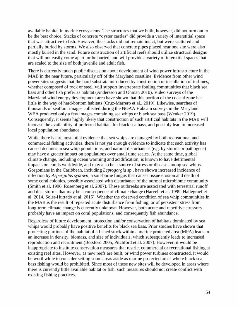
54

available habitat in marine ecosystems. The structures that we built, however, did not turn out to be the best choice. Stacks of concrete “oyster castles” did provide a variety of interstitial space that was attractive to fish. However, the stacks did not remain intact, but were scattered and partially buried by storms. We also observed that concrete pipes placed near one site were also mostly buried in the sand. Future construction of artificial reefs should utilize structural designs that will not easily come apart, or be buried, and will provide a variety of interstitial spaces that are scaled to the size of both juvenile and adult fish.

There is currently much public discussion about development of wind power infrastructure in the MAB in the near future, particularly off of the Maryland coastline. Evidence from other wind power sites suggests that the hard substrata introduced by construction or installation of turbines, whether composed of rock or steel, will support invertebrate fouling communities that black sea bass and other fish prefer as habitat (Andersson and Ohman 2010). Video surveys of the Maryland wind energy development area have shown that this portion of the coastal zone has little in the way of hard-bottom habitats (Cruz-Marrero et al., 2019). Likewise, searches of thousands of seafloor images collected during the NOAA Habcam surveys in the Maryland WEA produced only a few images containing sea whips or black sea bass (Wenker 2019). Consequently, it seems highly likely that construction of such artificial habitats in the MAB will increase the availability of preferred habitats for black sea bass, and possibly lead to increased local population abundance.

While there is circumstantial evidence that sea whips are damaged by both recreational and commercial fishing activities, there is not yet enough evidence to indicate that such activity has caused declines in sea whip populations, and natural disturbances (e.g. by storms or pathogens) may have a greater impact on populations over small time scales. At the same time, global climate change, including ocean warming and acidification, is known to have detrimental impacts on corals worldwide, and may also be a source of stress or disease among sea whips. Gorgonians in the Caribbean, including Leptogorgia sp., have shown increased incidence of infection by Aspergillus sydowii, a soil-borne fungus that causes tissue erosion and death of some coral colonies, possibly associated with disturbance of the normal microbiome community (Smith et al. 1996, Rosenberg et al. 2007). These outbreaks are associated with terrestrial runoff and dust storms that may be a consequence of climate change (Harvell et al. 1999, Hallegraef et al. 2014, Soler-Hurtado et al. 2016). Whether the observed condition of sea whip communities in the MAB is the result of repeated acute disturbance from fishing, or of persistent stress from long-term climate change is currently unknown. However, both acute and repetitive stressors probably have an impact on coral populations, and consequently fish abundance.

Regardless of future development, protection and/or conservation of habitats dominated by sea whips would probably have positive benefits for black sea bass. Prior studies have shown that protecting portions of the habitat of a fished stock within a marine protected area (MPA) leads to an increase in density, biomass, and size of individuals, which subsequently leads to increased reproduction and recruitment (Botsford 2005, Pitchford et al. 2007). However, it would be inappropriate to institute conservation measures that restrict commercial or recreational fishing at existing reef sites. However, as new reefs are built, or wind power turbines constructed, it would be worthwhile to consider setting some areas aside as marine protected areas where black sea bass fishing would be prohibited. Since most of these new sites will be developed in areas where there is currently little available habitat or fish, such measures should not create conflict with existing fishing practices.

55

References Andersson, M. H., and M. C. Ohman. 2010. Fish and sessile assemblages associated with wind-

turbine constructions in the Baltic Sea. Marine and Freshwater Research 61(6):642-650.

Botsford, L. W. 2005. Potential contributions of marine reserves to sustainable fisheries: Recent modeling results. Bulletin of Marine Science 76(2):245-260.

Cruz-Marrero, W., D. W. Cullen, N. R. Gay, and B. G. Stevens. 2019. Characterizing the benthic community in Maryland’s offshore wind energy areas using a towed camera sled: Developing a method to reduce the effort of image analysis and community description. PLoS ONE 14(5):e0215966.

Fabrizio, M. C., J. P. Manderson, and J. P. Pessutti. 2013. Habitat associations and dispersal of black sea bass from a mid-Atlantic Bight reef. Marine Ecology Progress Series 482:241-253.

Hallegraeff, G., and coauthors. 2014. Australian Dust Storm Associated with Extensive Aspergillus sydowii Fungal “Bloom” in Coastal Waters. Applied and Environmental Microbiology 80(11):3315-3320.

Harvell, C. D., K. Kim, J. M. Burkholder, R. R. Colwell, and et al. 1999. Emerging marine diseases--climate links and anthropogenic factors. Science 285(5433):1505-10.

Pitchford, J. W., E. A. Codling, and D. Psarra. 2007. Uncertainty and sustainability in fisheries and the benefit of marine protected areas. Ecological Modelling 207(2-4):286-292.

Rosenberg, E., O. Koren, L. Reshef, R. Efrony, and I. Zilber-Rosenberg. 2007. The role of microorganisms in coral health, disease and evolution. Nature Reviews. Microbiology 5(5):355-62.

Schweitzer, C. C., R. N. Lipcius, and B. G. Stevens. 2018. Impacts of a multi-trap line on benthic habitat containing emergent epifauna within the Mid-Atlantic Bight. ICES Journal of Marine Science:fsy109-fsy109.

Soler-Hurtado, M. M., J. V. Sandoval-Sierra, A. Machordom, and J. Diéguez-Uribeondo. 2016. Aspergillus sydowii and Other Potential Fungal Pathogens in Gorgonian Octocorals of the Ecuadorian Pacific. PLoS ONE 11(11).

Smith, G. W., L. D. Ives, I. A. Nagelkerken, and K. B. Ritchie. 1996. Caribbean sea-fan mortalities. Nature 383(6600):487.

Wenker, R. 2019. Sea Whip Coral (Leptogorgia virgulata) in the Mid-Atlantic Bight: Colony Complexity, Age, and Growth. MS Thesis. University of Maryland Eastern Shore. 51 Pages.

Appendix Photographs. Diving activities during the project: A-C, Cara Schweitzer setting up video tripods (Nick Caloyianis); D, Brad Stevens preparing to dive (Jeremiah Kogon).

A B C D

57

Quadrat photos taken at sites PH-S and PH-N. E) Quadrat with high abundance of boring sponge Cliona celata (yellow dots); F) Photo of wood wreck with black sea bass near center; G) Quadrat with moderate abundance of boring sponge and northern stone coral Astrangia poculata (white patches); H) Quadrat with high abundance of sea whips Leptogorgia virgulata.

E F G H

58

Tools of the Trade. I) Cara Schweitzer with video tripod; J) Digital camera on quadrat frame; K) Brad Stevens with “oyster castle” pyramids of 4-tiers each; L) A 2-tier pyramid with Cobia Rachycentron canadum in foreground.

I J K L

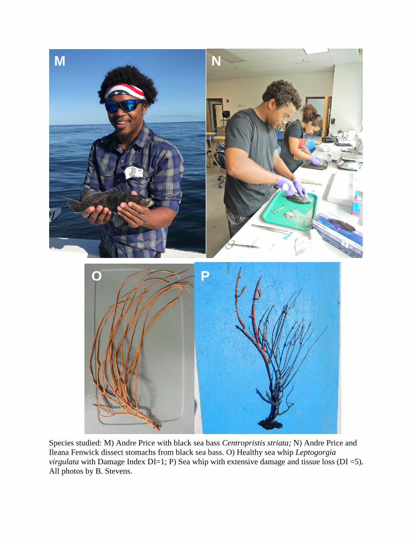
Species studied: M) Andre Price with black sea bass Centropristis striata; N) Andre Price and Ileana Fenwick dissect stomachs from black sea bass. O) Healthy sea whip Leptogorgia virgulata with Damage Index DI=1; P) Sea whip with extensive damage and tissue loss (DI =5). All photos by B. Stevens.

M N O P

60

The Authors Bradley G. Stevens, PhD Dr. Stevens is a tenured Professor of Marine Science in the Department of Natural Sciences at the University of Maryland Eastern Shore, and Distinguished Research Scientist with the NOAA Living Marine Resources Cooperative Science Center. He received his PhD from the University of Washington in 1982. He previously worked for the National Marine Fisheries Service of NOAA for 22 years in Kodiak, Alaska, where he was Task Leader for Bering Sea Crab Stock Assessment, managed the Seawater Laboratory at the Kodiak Fisheries Research Center, and was Acting Director of the NMFS Kodiak Laboratory in 2006. He has authored or co-authored over 65 peer-reviewed publications and conference proceedings, and is the Editor and principal author of “King Crabs of the World”, CRC Press, 2014. Dr. Stevens’ research program focuses on ecology and reproductive biology of invertebrates (primarily crabs), and impacts of fishing on fish and invertebrate populations and their habitats. In 2003, he discovered the wreck of the Russian barque Kad’yak, the oldest known shipwreck site in Alaska, and the first shipwreck from the Russian Colonial Period ever found, and recently published an account of that discovery: “The Ship, the Saint, and the Sailor: The Long Search for the Legendary Kad'yak” (Ingram Press, 2018). In 2015, he initiated the AAUS Diving program at UMES, and currently serves on the University System of Maryland Diving Control Board.

Cara Schweitzer, PhD. Dr. Cara Schweitzer received her PhD in Marine, Estuarine and Environmental Science from the University of Maryland Eastern Shore in May, 2019. The title of her PhD Dissertation was “The Effects of Commercial Trap Fishing on Benthic Structural Habitat and Fish Abundance in the Mid-Atlantic: Case Study of Black Sea Bass Centropristis striata”. She is currently weighing offers for postdoctoral employment.

Andre L. Price Mr. Andre Price received his MS Degree in Marine, Estuarine and Environmental Science from the University of Maryland Eastern Shore in May, 2019. The title of his Thesis was “Comparing Localized Feeding Ecology of Black Sea Bass (Centropristis striata) at Natural and Artificial Reefs Using Gut Content and Stable Isotope Analyses”. He currently works for the National Marine Fisheries Service, Northeast Fishery Science Center, in Woods Hole, MA.