IOTC-WPTT-2006-22

Updated stock assessment of bigeye tuna (Thunnus obesus) resource in the Indian Ocean by the age structured production model(ASPM) analyses

(1960-2004)

Tom Nishida and Hiroshi Shono

National Research Institute of Far Seas Fisheries (NRIFSF)

Fisheries Research Agency 5-7-1, Orido, Shimizu-Ward, Shizuoka-City, Shizuoka, Japan 424-8633

July, 2006

Abstract We updated the stock assessment of the bigeye tuna (BET) resource in the Indian Ocean using the age-structure production model (ASPM) with 45 years data from 1960-2004. It is resulted that MSY=97,415 tons and the stock is continuing at the over-fishing status because (a) the catch levels exceeded the MSY level in past ten years (1993-2004), (b) current to virgin levels of total & spawning stock biomass (SSB) were 0.36 and 0.53 (well below from 1, the critical level to keep MSY) respectively and (c) F & SSB (MSY) ratios (current levels to MSY) have been rapidly reaching to the critical level, i.e., 1 to sustain the MSY level. For this time, we could successfully estimate 90% confidence intervals for the various population parameters evaluated in the ASPM using the bootstrap experiments. Based on the comparative studies of four ASPM results in the past (2002, 2004, 2005 and 2006), it is likely that consistent and robust results have been evaluated in the past by the ASPM while there is a number of uncertainties described in the past IOTC WPTT reports. Contents

1. Introduction---------------------------------------------------------------------------------------------------- 2

2. ASPM

2.1 INPUT-------------------------------------------------------------------------------------------- 2-5

2.2 Sensitivity for selectivity and Rho--------------------------------------------------------- 6

2.3 ASPM runs-------------------------------------------------------------------------------------- 7-10

2.4 Confidence intervals by bootstraps------------------------------------------------------- 11-12

3. Comparisons among ASPM results (2002, 2004, 2005 & 2006) ------------------------------- 13-14

4. Discussion----------------------------------------------------------------^----------------------------------- 15-16

Acknowledgements----------------------------------------------------------------------------------------------- 16

References--------------------------------------------------------------------------------------------------------- 16

_________________________________________________________________________ Submitted to the IOTC Eighth working party on the tropical tuna meeting（WPTT） (July 24-28, 2006), Victoria, Seychelles

1

1. Introduction In this paper, we updated the stock assessment of the bigeye tuna (BET) resource in the Indian Ocean using the age-structure production model (ASPM). The ASPM was used because this approach was recommended for the BET stock assessment in the IOTC ad hoc Working Party meeting on Methods (WPM) held in IRD, Sète, France 23-27, April, 2001 (Anonymous, 2001). The primary reason for the IOTC Ad hoc WPM meeting recommended is that there are not enough season-area specific size data to conduct age based approach such as VPA, while the ASPM can be conducted without such specific size data. Consequently, results by the ASPM have been accepted by the IOTC WPTTs and Scientific Committees in the past four years and used in Executive Summaries. For this time, we conducted the ASPM analyses for 45 years (1960-2004) by assuming again that BET in the Indian Ocean forms a single stock. We did not use the earlier data in 1950s by the following reasons: The Japanese (bigeye) tuna fishing grounds were limited in the eastern Indian Ocean in 1950s and not fully expanded to the entire Indian Ocean. When many un-fished fishing grounds were included in the catch rates analyses, results such as the abundance trends will be seriously biased (Walters, 2003 or IOTC-2006-INF02). Thus we exclude the data in 1950s and used the data from 1960 after the Japanese longline fishing grounds were fully expanded to the entree the Indian Ocean.

2. ASPM 2.1 Input We used the ASPM software developed by Victor Restrepo (1997) called as ASPMS (stochastic version of ASPM). Input data of the ASPM (Catch, Biological, Selectivity and Index) are explained as follows: (1) Catch The bigeye catch by gear type were obtained from the IOTC database (May, 2006). Fig.1 and Table 1 show the trend of the catch (1950-2004).

B ET C atch (Indian O cean) (1950-2004)

0

50

100

150

1950 1960 1970 1980 1990 2000

1000 tons

O T H

P S

LL

Fig. 1 Trend of the bigeye catches in the Indian Ocean (1950-2004) (IOTC database, as of May 2006) Note: LL: tuna longline fisheries, PS: tuna purse seine fisheries, OTH: Other fisheries (Gillnet, troll, pole & line and handline)

2

Table 1 Catch statistics of bigeye tuna in the Indian Ocean (tons)(IOTC database, as of May 2006)

(tons)

Year LL PS O THERS TO TAL

1950 0 0 1 11951 0 0 1 11952 280 0 1 2811953 1,653 0 0 1,6531954 6,850 0 0 6,8501955 9,739 0 0 9,7391956 12,846 0 0 12,8461957 11,991 0 0 11,9911958 11,655 0 0 11,6551959 9,868 0 0 9,868

1960 16,115 0 1 16,1161961 14,951 0 1 14,9521962 18,482 0 1 18,4831963 13,303 0 1 13,3041964 18,025 0 1 18,0261965 19,538 0 1 19,5391966 24,129 0 1 24,1301967 24,762 0 1 24,7631968 39,501 0 1 39,5021969 30,427 0 2 30,429

1970 27,753 0 84 27,8371971 22,959 0 52 23,0111972 19,994 0 62 20,0561973 17,419 0 131 17,5501974 28,351 0 128 28,4791975 37,670 0 104 37,7741976 28,543 0 144 28,6871977 35,908 0 163 36,0711978 50,541 5 122 50,6681979 33,476 1 137 33,614

1980 34,862 21 109 34,9921981 34,834 13 235 35,0821982 43,380 116 112 43,6081983 49,510 587 200 50,2971984 39,684 4,020 375 44,0791985 44,868 7,159 338 52,3651986 46,704 10,626 498 57,8281987 51,224 13,400 445 65,0691988 57,053 15,057 2,257 74,3671989 56,656 11,980 836 69,472

1990 60,474 12,667 546 73,6871991 60,834 15,623 700 77,1571992 60,165 11,259 456 71,8801993 85,447 16,013 556 102,0161994 90,643 18,880 664 110,1871995 89,803 28,382 1,233 119,4181996 101,461 24,529 906 126,8961997 112,429 33,965 928 147,3221998 112,104 28,334 936 141,3741999 108,636 40,658 1,161 150,455

2000 98,372 29,859 641 128,8722001 90,289 23,717 1,005 115,0112002 104,647 29,042 1,235 134,9242003 99,768 22,946 1,272 123,9862004 102,629 22,586 1,300 126,515

Note: LL: tuna longline fisheries, PS: tuna purse seine fisheries, OTH: Other fisheries (Gillnet, troll, pole & line and handline)

3

(2) Biological parameters

ASPM requires 4 types of age-specific biological inputs, i.e., weights at the beginning and the mid

year, natural mortality (M) and the fecundity. We used 9 age classes from age 0-8+. These inputs

are obtained as follows:

Weight-at-age

Weight-at-age in the beginning and the mid year are estimated based on the following growth

equations and the length-weight relationship. The same age-weight key based on this information

and developed by IOTC (2003) was used (Table 2).

● L-W relationship

For fork length < 80 cm: W = (2.74 x 10-5)l2.908 Poreeyanond (1994) (Indian Ocean)

For 80cm <=fork length: W = (3.661x10-5 )l2.90182 Nakamura and Uchiyama (1966) (Pacific Ocean)

● Growth equation by Stequart and Conrad (2003)

[ ]( )0 .3 2 ( 0 .3 3 6 )( ) 1 6 9 1 t

t cmL e − − −= −

Natural mortality (M)

In the past we have applied two different M vectors used by ICCAT and SPC but we have learned

that the ICCAT M vector produced better fits to the model (IOTC, 2004). Hence we used the ICCAT

M vector (Table 2).

Fecundity

We assume that fecundity is proportional the body weight at the middle of each age and also

assume 0 fecundity for age 0-2 and 50% of fecundity for age 3 as in Table 2:

Table 2 Biological input parameters (*) used in the ASPM analyses Age 0 1 2 3 4 5 6 7 8

ICCAT 0.8 0.8 0.4 0.4 0.4 0.4 0.4 0.4 0.4

(beg) 0.00011 0.00386 0.01670 0.03160 0.04658 0.05994 0.07107 0.07993 0.08679 Weight

(ton) (mid) 0.00123 0.00786 0.02398 0.03922 0.05352 0.06580 0.07577 0.08359 0.08958

Maturity(*) 0 0 0 0.5 1 1 1 1 1

Fecundity 0 0 0 0.0196 0.05352 0.06580 0.07577 0.08359 0.08958

(*) Maturity is listed as reference and it is not the input parameter.

4

(3) Selectivity The selectivity-at-age for longline and purse seine fisheries (log and free school combined) were estimated using the growth curve by Stequart (2003) and separable VPA during the WPTT meeting in 2004. For this time we used the same selectivities. As suggested by Miyabe (2001), longline fisheries were divided by three periods (before 1976, 1977-91 and after 1992) due to their heterogeneity characteristics. Table 3 summarizes the selectivity. Table 3 Selectivity used for the ASPM analyses

M Fishery/Age 0 1 2 3 4 5 6 7 8 LL(1960-1976) 0 0.043 0.254 0.565 0.855 1 0.949 0.725 0.725 LL(1977-1991) 0 0.042 0.344 0.799 1 0.921 0.751 0.529 0.529 LL(1992-2002) 0 0.050 0.473 0.930 1 0.877 0.716 0.475 0.475

I C C A T

PS(1960-2002) 0.673 1 0.484 0.387 0.346 0.246 0.122 0.048 0.025

(4) Standardized CPUE We used Japanese and Taiwanese standardized (STD) CPUEs in the whole Indian Ocean estimated by Okamoto and Shono (2006) and Hsu (2006) which details are available in two other documents presented in this meeting (IOTC-WPTT-2006-__ and ___) respectively (Fig. 2). We used the Japanese STD CPUE as a base case, while Taiwanese STD CPUE for sensitivity attempts.

All Indian

0.00.20.40.60.81.01.21.41.61.82.0

1960 1964 1968 1972 1976 1980 1984 1988 1992 1996 2000 2004Years

Rel

ativ

e C

PUE Taiwan

Japan

Fig. 2 Standardize CPUE of Japan (1960－2004) and Tawain (1968-2004) (scaled as the average

values of eaach CPUE=1)

5

2.2 Sensitivity for steepness and Rho

We set the ASPM run for the Japanese STD CPUE (1960-2004) as a base case. As we have been

facing the unrealistic steepness value (0.999) estimated in the past ASPM runs. To solve this

problem, late Dr Geoff Kirkwood (past SC and WPTT Chairs) suggested to fix its values to test

sensitivity. For this time, we followed his suggestion to test sensitivity by varying the selectivity from

0.7, 0.8 to 0.9.

In addition according to our last ASPM paper in 2005 submitted to the SC in 2005 (IOTC-SC-2005-

INF10), we learned that results of ASPM were influenced by Rho values (values used to reduce

biases caused by auto-correlation errors in the spawner-recruit relationship). Rho is one of the

input parameters in the ASPM. In the last analyses we had Rho=0.07 as the best. Thus for this time,

we also test its sensitivities by varying the ranges of Rho from 0.0 to 0.40 by 0.1 step size.

In the sensitivity analyses we use four criteria to evaluate the best parameters, -in (likelihood), R

squared, CV (Virgin Biomass) and CV [SSB(virgin) to SSB(2004) ratio] obtained from the ASPM

outputs. Table 4 shows result of the sensitivity analyses which indicated that Rho=0.1 is the best

value and steepness=0.7 is the best value although there are not so much differences with others.

Table 4 Result of the sensitivity analyses for the steepness and Rho in the ASPM

NC: no convergence ; yellow marked values means the best one in each criterion.

Steepness Rho -ln (likelihood)

R squared

C V (Virgin Biom ass)

C V SSB(virgin) to SSB(2004) ratio

Decision

0 NC

0.1 -129.8 0.900 0.292 4.002 Best & selected

0.2 -129.8 0.899 0.304 9.552

0.3 NC

0.7

0.4 NC

0 NC

0.1 -129.8 0.900 0.292 4.006

0.2 -129.8 0.899 0.312 9.623

0.3 NC

0.8

0.4 NC

0 NC

0.1 -129.8 0.900 0.292 4.006

0.2 -129.8 0.899 0.312 9.623

0.3 NC

0.9

0.4 NC

6

2.3 ASPM runs

Setting the ASPM run with Japanese STD CPUE (1960-2004) as a base we made five other ASPM

runs for sensitivities by combining Japan and Taiwan STD CPUE and two different periods (1960-

2004 and 1968-2004) as shown in Table 5. As results of six ASPM runs, all runs were properly

converged and the base case (Run 1) was resulted to produce the most reasonable and robust

estimates. Figs. 3-11 depict results of Run 1.

Table 5 SIX ASPM runs: INPUTS & RESULTS BASE

CASE SENSITIVITIES

Run 1 2 3 4 5 6 INPUT DATA (whole Indian Ocean)

Catch LL and PS LW Poreeyanond (1994) & Nakamura/Uchiyama (1966)

Growth Stequart (2003) Selectivity LL (3 periods) and PS (log & free school combined)

S-R Beaverton-Holt model M vector ICCAT type

ASPM parameters steepness=0.7 rho=0.1 Period (a) 1960-2004 (b) 1968-2004

Standardized CPUE

Japan Taiwan Japan & Taiwan

Japan Taiwan Japan & Taiwan

RESULTS Results of ASPM

Converged

ln(likelihood)

-130 -113 -172 -106 -106 -150

R-squared

0.91 0.85 0.68 0.91 0.85 0.67

MSY

9. 74 12.1 12.6 9.98 11.8 12.6

7

Catch (2004) 12.6 VirginSSB(million t)

at (a) 1960 (b) 1978 1.06 1.34 1.46 1.05 1.31 1.39

SSB(MSY) 0.32 0.41 0.42 0.33 0.41 0.42 SSB(2004) 0.38

0.73 0.66 0.39 0.72 0.67

SSB(MSY) ratio

=SSB2004/SSB(MSY)

1.19 1.78 (too high/ optimistic)

1.57 (too high/ optimistic)

1.12 1.76 (too high/ optimistic)

1.60 (too high/ optimistic)

SSB(VIRGIN) ratio

=B2004/B(a) or (b)

0.36 0.54 0.45 0.37 0.55 0.48

F(MSY) 0.32 0.29 0.30 0.32 0.29 0.30 F(2004) 0.32 0.18 0.20 0.31 0.19 0.20 F(ratio)

=F2004/F(MSY) 1.00 0.62

(too low/ optimistic)

0.67 (too low/

optimistic)

0.97 0.66 (too low/

optimistic)

0.67 (too low/

optimistic) DECISION Best

run Un realistic

(too optimistic)

Un realistic

(too optimistic)

Secondbest

Un realistic

(too optimistic)

Un realistic

(too optimistic)

(10,000 tons)

O verall F vs F(M SY )

0

0.2

0.4

0.6

1960 1965 1970 1975 1980 1985 1990 1995 2000

F

F(M SY)

Fig. 3 Trends of overall F vs. F(MSY)

C atch vs M SY

0

50000

100000

150000

200000

1960

1962

1964

1966

1968

1970

1972

1974

1976

1978

1980

1982

1984

1986

1988

1990

1992

1994

1996

1998

2000

2002

2004

tons

C atch

M SY

Fig. 4 Trends of catch vs. MSY

S S B vs S S B (M SY )

0.0

0.5

1.0

1.5

1960 1965 1970 1975 1980 1985 1990 1995 2000

million tons

S S B

S S B (M S Y )

8

Fig. 5 Trends of mature biomass vs. mature biomass (MSY) M ature and im m ature biom ass

0.0

0.5

1.0

1.5

1960 1965 1970 1975 1980 1985 1990 1995 2000

million ton

sim m ature

m ature

Fig. 6 Trends pf biomass (mature and immature)

trend of num be of fish by age

0

50

100

150

200

250

1960

1963

1966

1969

1972

1975

1978

1981

1984

1987

1990

1993

1996

1999

2002

million fish

age 4+

age 3

age 2

age 1

age 0

Fig. 7 Trends of number of fish by age

9

T rend of recruit (w eight)

0

50

100

150

1960 1965 1970 1975 1980 1985 1990 1995 2000

1000 tons

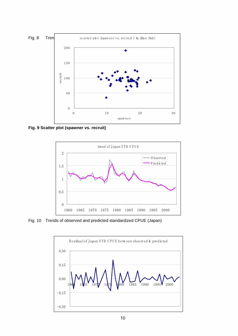
Fig. 8 Trend of recruitment scatter plot (spaw ner vs. recruit ) (m illion fish)

0

50

100

150

200

0 10 20 30

spaw ner

recruit

Fig. 9 Scatter plot (spawner vs. recruit)

trend of Japan ST D C PU E

0

0.5

1

1.5

2

1960 1965 1970 1975 1980 1985 1990 1995 2000

O bserved

Predicted

Fig. 10 Trends of observed and predicted standardized CPUE (Japan)

R esidual of Japan S TD C PU E betw een observed & predicted

-0.30

-0.15

0.00

0.15

0.30

1960 1965 1970 1975 1980 1985 1990 1995 2000

10

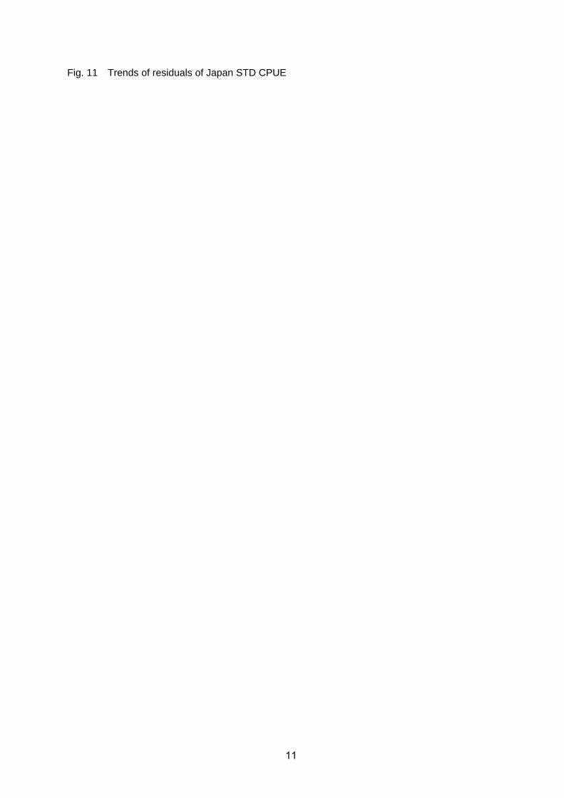
Fig. 11 Trends of residuals of Japan STD CPUE

11

2.4 Confidence intervals (CI) by bootstraps

IMPORTANT NOTE

In the past BET assessments by the ASPM, we could not get the reasonable confidence intervals.

We thought that the cause of this problem was due to the program structure problem in the ASPM.

But for this time, we re-examined our macro programs and procedures to compute the CI. Then we

found a few errors (bugs) in our macro programs to link among ASPM, excel and batch

procedures. After we corrected these bugs, we realized that the revised programs and procedures

could provide the reasonable CI.

Based on the updated ASPM result (Run 1) using the revised macro programs and procedures, we

estimated the confidence interval of the MSY using 330 times of the bootstrap experiments by

adding the random noises into CPUEs and the Spawner-Recruit relations. The methods are

described as below:

Methods

ASPM parameters

(a) Add the normal random numbers into the Japanese standardized CPUEs (1960-2004);

(b) Do 330 times of the ASPM Runs using the 330 sets of the CPUE created in (a);

(c) Get 330 S-R relations (B-H model) from the 330 times of the ASPM runs;

MSY for the additional steps

(d) Using each S-R relation with the age specific selectivity (from the ASPM results), estimate MSY

by optimizing age specific F.

(e) Repeat (d) 330 times and get 330 MSY values;

(f) Estimate SE then compute confidence intervals based on 330 MSY values.

Although we attempted 330 times bootstraps, we could get the convergences only for 124 times.

Using 124 results, we computed SE and 90% CI.

Table 6 shows the summary of points and the confident intervals for MSY and various ASPM parameters based on the bootstraps.

11

Table 6 Summary of estimated CI for MSY and various ASPM parameters based on the bootstraps.

Unit 90% lower CI Point estimates 90% upper CI

[MSY]

MSY tons

79,840 97, 415

(SE=9,250)

114,990

[TB: Total Biomass]

TB(1960) 1.31

TB(2004)

million

tons

0.69

TB(MSY) ratio

(2004 to MSY)

rate

between 0 & 1

0.42 0.53

(SE=0.06)

0.64

[SSB]

SSB(MSY) 0.32

SSB(1960) 1.06

SSB(2004)

million

tons

0.38

SSB(MSY) ratio

(2004 to MSY)

0.85 1.19

(SE=0.18)

1.53

SSB(virgin) ratio

(2004 to 1960)

rate

between 0 & 1 0.27 0.36

(SE=0.05)

0.45

[F]

F(MSY) 0.32

F(1960) 0.02

F(2004)

instantaneous

annual mortality

rate

0.32

F(MSY) ratio

(2004 to MSY)

rate

between 0 & 1

0.20

1.00

(SE=0.20)

1.38

12

3. Comparisons among ASMP results (2002, 2004, 2005 and 2006) Table 7 and Figs. 12-14 show summaries of the comparisons among ASPM results in the past, i.e.,

WPTT4 (2002), WPTT6 (2004), SC8 (2005) and WPTT8 (2006).

Table 7 Summary of comparisons among ASPM results (2002, 2004, 2005 and 2006)

Year assessed 2002

(WPTT4)

2004

(WPTT6)

2005

(SC8)

2006

(WPTT8)

Method (software) ASPMS (software created by Restrepo,1997)

Period analyzed 1960-1999

(40 years)

1960-2002

(42 years)

1960-2003

(44 years)

1960-2004

(45 years)

Area Whole Indian Ocean

Catch LL and PS

LL (3 periods) and PS (2 periods) Selectivity

(estimated by separable VPA) Miyabe et al

(2002)

WPTT6

(2004)

CPUE

(Okamoto et al)

Japan

(1960-1999)

Japan

(1960-2002)

Japan

(1960-2002)

Japan

(1960-2004)

M vector ICCAT type:0.8 (age 0-1) and 0.4 (age 2-8)

S-R Beaverton-Holt model

steepness 0.99

(estimated)

0.99

(estimated)

0.99

(estimated)

0.70

(fixed)

LW Poreeyanond (1994) (less than 80cm) & Nakamura/Uchiyama (1966) (80cm or larher)

Growth Tankevich

(1982)

Stequart and Conrad (2003)

MSY(Point)

[90% CI]

101,522 96,858 99,212 97, 415

[79,840-114,990]

current catch

(tons)

150,455

(1999)

123,942

(2002)

123,986

(2003)

126,515

(2004)

MSY

(tons)

90 % CI NA

TB Total

biomass

TB (virgin) ratio

=TB(current)/TB(virgin)

[90% CI]

0.61 0.50 0.49 0.53

[0.42-0.64]

SSB(virgin) ratio

=SSB(current)/SSB(virgin)

[90% CI]

0.51 0.36 0.28 0.36

[0.27-0.45]

SSB(MSY) ratio

=SSB(current)/SSB(MSY)

[90% CI]

2.34 1.56 1.20 1.19

[0.85-1.53]

SSB

Spawning

stock

biomass

F ratio

=F(current)/F(MSY)

[90% CI]

0.66 0.98 0.89 1.00

[0.62-1.36]

13

M SY and C atch

0

50000

100000

150000

200000

W PTT4(2001) W PTT7(2004) SC (2005) W PTT8(2006)

tons

C atch

upper C I

M S Y

low er C I

Fig. 12 Trend of estimated MSY and catch evaluated in the past four BET stock assessments by ASPM.

Fig. 13 SSB (MSY) ratio (current to MSY) Fig. 14 F (MSY) ratio (current to MSY)

14

F (M SY) ratio

0

0.5

1

1.5

2

W PTT4(2001) W PTT7(2004) SC (2005) W PTT8(2006)

upper C I

F ratio (M SY)

low er C I

Trend of SSB ratio (current to M SY)

0

1

2

3

W PTT4(2001) W PTT7(2004) SC (2005) W PTT8(2006)

upper C I

SSB ratio (M SY)

low er C I

Total biom ass ratio (current vs. virgin)

0.5

1

upper C I

TB ratio (virgin)

low erC I

OVERE

SSB (virgin) ratio(current to virgin)

0.5

1

upper C I

SSB ratio (virgin)

lower C I

Fig. 15 SSB (virgin) ratio (current to virgin) Fig. 16 TB (virgin) ratio (current to virgin)

15

4. Discussion

(1) Taiwan STD CPUE

It is the first time that the trends of the standardized Taiwan CPUE became very similar to the

Japanese one, especially in recent years unlike in the past. This caused that the all the ASPM even

with Taiwan STD CPUE could get conversions and provided reasonable results, unlike in the past,

i.e., the ASPM with Taiwan could not get conversion and even if conversion were made, the

estimated parameters were un-realistic. This implies that Taiwan STD CPUE for this time is

improved than those in the past.

However even with the improved Taiwan STD CPUE, it was resulted that the ASPM results with

Japan STD CPUE showed slightly better fits to the model and provided more realistic results.

(2) Sensitivity analyses for steepness and Rho

We have been facing the unrealistic steepness value (0.999) estimated in the past ASPM runs. To

solve this problem, we fixed its values to test sensitivity. In addition according to our last ASPM

paper in 2005 submitted to the SC in 2005(IOTC-SC-2005-INF10), we learned that results of ASPM

were influenced by Rho values (values used to reduce biases caused by auto-correlation in the

spawner-recruit relationship). Thus we also tested its sensitivities. As a result we get Rho=0.1 and

steepness=0.7 as the best value although there are not so much differences with other testing

values in terms of criteria.

(3) Confidence intervals (CI)

In the past BET assessment by the ASPM, we could not get the reasonable confidence intervals.

We thought that the cause of this problem was due to the program structure problem in the ASPM

(see IOTC-SC-2005-INF10). But for this time, we re-examined our macro programs and procedures

to compute the CI. Then we found a few errors in our macro programs to link among ASPM, excel

and batch procedures. After we corrected these bugs, we realized that the revised programs and

procedures could provide the reasonable CI.

(3) Comparison of the past ASPM results

Based on the comparative studies of four ASPM results in the past (2002, 2004, 2005 and 2006), it is likely that consistent and robust results have been evaluated in the past by the ASAM (see Table 7 & Figs. 12-14), while there is a number of uncertainties described in the past IOTC WPTT reports

16

(4) Suggestion to resources managements

For this time, we could obtain similar ASPM results in the past which indicated again that stock

has been continuing the over-fishing status and furthermore BET stock status has become more

pessimistic because (a) the catch levels exceeded the MSY level (97,415 tons) in past ten years

(1993-2004), (b) current to virgin levels of total & spawning stock biomass (SSB) were 0.36 and

0.53 (well below from 1, critical level to keep MSY) respectively and (c) F & SSB (MSY) ratios

(current levels to MSY) have been rapidly reaching to the critical level. Based on these clear and

consistent facts obtained in the past 4 ASPM assessments we strongly recommend that all catch

and fishing effort for any gears should be reduced to the MSY level immediately.

Acknowledgements and Condolences

We thank late Geoff Kirkwood to suggest us to improve the ASPM runs. Taking this opportunity we

would like to express our sincere condolences on his sudden passing away in last March. Further

we here acknowledge Geoff’s great leaderships and excellent supervisions to our past WPTT and

SC as Chairs. Special thanks are towards Victor Restrepo (ICCAT) to assist to solve the ASPM

structure problems.

References Anonymous (2001) Report of the IOTC ad hoc working party on methods, Sète, France 23-27, April,

2001: 20pp.

Hsu (2006) Standarization of bigeye tuna CPUE of Taiwanese longline fisheris (IOTC-WPTT-2005-

__): __pp.

IOTC (2006): IOTC nominal catch database (excel files provided Miguel Herrera), May, 2006.

IOTC (2003): Report of the WPTT5. __pp.

IOTC, (2004): Report of the WPTT6. __pp.

Miyabe, N. (2001) Estimation of selectivity at age for bigeye tuna in the Indian Ocean,

(IOTC/WPTT/01/20): 13pp.

Nakamura, E.L. and Uchiyama J.H. (1966) Length-weight relations of Pacific tunas. In proc,

Governor’s Conf. Cent. Pacify. Fish. Resources, edited by T.A. Manar, Hawaii: 197-201.

17

Nishida, T. (Editor) for the IOTC Scientific Committee Working Group. Updated BET stock

assessment: Report on the requests to the Scientific Committee raised by the 9th

Commissioner meeting (2005) regarding Resolution 05/01 (Conservation and

management measure for bigeye tuna) (OTC-2005-SC-INF10) 15pp

Okamoto and Shono (2006) Japanese longline CPUE for bigeye tuna in the Indian Ocean up to

2004 standardized by GLM applying gear material information in the model (IOTC-WPTT-

2006-___).

Poreeyanond, D. (1994) Catch and size groups distribution of tunas caught by purse seining survey

in the Arabian Sea, Western Indian Ocean, 1993. In Ardill, J.D. [ed.] Proceedings of the

Expert Consultation on Indian Ocean Tunas, 5th Session, Mahé, Seychelles, 4-8 October

1993, 275 p., IPTP Col. Vol. 8 : 53-54

Restrepo, V. (1997) A Stochastic implementation of an Age-Structured Production Model (ASPMS)

(ICCAT/SCRS/97/59) and Users Guide: 23pp.

Stequart , R. and Conand, F. (2003) Age and growth of Bigeye tuna in the western

Indian Ocean. IOTC/WPTT-03-Info2

Tankevich, P.B. (1982) Age and growth of the bigeye tuna, Thunnus obesus (Scombridae) in the

Indian Ocean. J. Ichthyology. 22(4): 26-31.

Walters, C., 2003. Folly and fantasy on the analysis of spatial catch rate data. Can. J. Fish. Aquat.

Sci. 60, 1433–1436 (or IOTC-2006-WPTT-INF02).

18

IOTC-2006-WPTT8-22 (Addendum 3)

Updated stock assessment of bigeye tuna (Thunnus obesus) resource

in the Indian Ocean by the age structured production model(ASPM) analyses (1960-2004)

Tom Nishida and Hiroshi Shono Addendum D Results of the ASPM run for the final and agreed base case---- Addendum E Results of the future projection for the base case ----------------- Table 10 Results of the ASPM run for the final and agreed base case

Base case M1 [90% CI]

M2

INPUT

STD CPUE Japan (1960-2004) Steepness 0.80 (fixed) Rho 0.10 (fixed)

OUTPUT

Criteria for goodness of fit

ln(likelihood) -129.75 -131.08 -131.21 R-squared 0.900 0.907 0.907 CV (virgin biomass) 0.292 0.287 0.311 CV (B1 ratio) 4.002 3.286 3.683

MSY vs. Catch MSY(tons) 97,415 99,244

[82,718-115,770] 104,063

Catch (2004) 126,518 TB: Total biomass

TB (1960: virgin) (million tons) 1.31 1.38 1.26 TB (2004: current) (million tons) 0.69 0.72 0.70 TB (virgin) ratio (current to virgin) 0.53 0.52

[0.41-0.63] 0.56

SSB: Spawning stock biomass SSB(1960: virgin) (million tons) 1.06 1.15 1.02 SSB (2004: current) (million tons) 0.38 0.43 0.40 SSB(MSY) (million tons) 0.32 0.35 0.32 SSB (MSY) ratio (current to MSY) 1.19 1.23

[0.91-1.55] 1.14

SSB(virgin) ratio (current to virgin) 0.36 0.37 [0.28-0.47]

0.39

F: Instantaneous fishing mortality F(2004: current) 0.32 0.29 0.30 F(MSY) 0.32 0.30 0.33 F ratio (current to MSY) 1.00 0.97

[0.57-1.37] 0.91

Comments The best fit (Based on criteria)

20

Addendum E Results of the future projection for the base case (point estimates)

20

Catch control

F control

Constant catch at the 2004 level (LL= PS= )

Constant F at the 2004 level (LL= PS= )

Constant catch at the 2004 level (LL= PS= )

Constnat Catch

0

0.5

1

1.5

1990 1995 2000 2005 2010 2015

million fish

SSB

TB

SSB (M SY)

Constnat Catch

0

0.5

1

1.5

1990 1995 2000 2005 2010 2015

million fish

SSB

TB

SSB (M SY)

20

IOTC-2006-WPTT8-22 (Addendum 3)

Updated stock assessment of bigeye tuna (Thunnus obesus) resource

in the Indian Ocean by the age structured production model(ASPM) analyses (1960-2004)

Tom Nishida and Hiroshi Shono Addendum D Results of the ASPM run for the final and agreed base case---- 21 Addendum E Results of the future projection for the base case ------------------ 22 Addendum F Comparisons among results by 5 SA methods (for discussion)----- 23-24 Table 10 Results of the ASPM run for the final and agreed base case

21 21

Final base case M1 [80% CI]

to be provided in July 28(Fri) INPUT

STD CPUE Japan (1960-2004)

Steepness

0.80 (fixed)

Rho 0.10 (fixed)

OUTPUT

MSY vs. Catch MSY(tons) 111,195

[xx.xxx – xxx.xxx］ Catch (2004) 126,518

TB: Total biomass TB (1960: virgin) (million tons) 1.38 TB (2004: current) (million tons) 0.72 TB (virgin) ratio (current to virgin) 0.52

[0.xx-0.xx] SSB: Spawning stock biomass

SSB(1960: virgin) (million tons) 1.15 SSB (2004: current) (million tons) 0.43

SSB(MSY) (million tons) 0.32 SSB (MSY) ratio (current to MSY) 1.34

[0.xx-1.xx] SSB(virgin) ratio (current to virgin) 0.39

[0.xx-0.xx] F: Instantaneous fishing mortality

F(2004: current) 0.29 F(MSY) 0.36 F ratio (current to MSY) 0.81

[0.xx-1.xx]

Addendum E Results of the future projection for the base case (point estimates)(2005-2015) Catch control F control

(Y-scale : million tons )

Current catch in 2004 (LL=102,866 tons and PS=23,628 tons)

Current F in 2004(F=0.293)

0

1

2

1990 1995 2000 2005 2010 2015

SSB

TB

SSB(M SY)

0

1

2

1990 1995 2000 2005 2010 2015

SSB

TB

SSB (M SY)

10% reduction of the current 2004 catch (LL=92,597 tons and PS=21,266 tons )

Average F (2000-2002) (F=0.265)

22 21

]

Average F (1998-2001)(F=0.251)

0

1

1990 1995 2000 2005 2010 2015

2 SSB

TB

SSB(M SY)

0

1

2

1990 1995 2000 2005 2010 2015

SSB

TB

SSB(M SY)

0

1

2

1990 1995 2000 2005 2010 2015

SSB

TS

SSB (M SY)

22

23 21

SSB(current to M SY ratio

0

1

2

ASPM SS2 ASPIC C ASAL spB ayes

(1960-2004) (1960-2004) (1960-2004) (1950-2004) (1952-2004)

) SSB atM SY

M SY

0

50

100

150

200

ASPM SS2 ASPIC C ASAL spB ayes

(1960-2004) (1960-2004) (1960-2004) (1950-2004) (1952-2004)

current catch(2004)(127,000 ton)

F (M SY) ratio

0

0.5

1

A SPM SS2 A SPIC C A SA L spBayes

(1960-2004)

(1960-2004)

(1960-2004)

(1950-2004)

(1952-2004)

SSB(1960 to current) ratio

0

0.5

1

ASPM SS2 ASPIC CA SA L spB ayes

(1960-2004)

(1960-2004)

(1960-2004)

(1950-2004)

(1952-2004)

45 years (1960-2004)

55 years 1950s-2004

23

catch vs M SY by m ethods

0

100

200

1950

1953

1956

1959

1962

1965

1968

1971

1974

1977

1980

1983

1986

1989

1992

1995

1998

2001

2004

catch

A SPM

SS2

A SPIC

C A SA L

sp B ayes

COMMENTS

If we accept the results of all 5 methods, we face uncertainty to interpret the results.

The results are different by the period of the analyzed years, i.e., analyses by the shorter period data (1960-2004) [ASPM, SS2 and ASPIC] produced more conservative results than those by the longer period of the data (1950s-2004) [CASAL and spays].

The current catch [127,000 tons] is around MSY [111,000-137,000] for all cases. In most

conservative case [ASPM] the catch is above MSY for 10 years since 1993. While the least conservative case [CASAL] catch were above only for 3 years.

In all the cases, the current SSB is the less than a half of the 1960 level (virgin level for the ASPM,

SS2 and ASPIC). This suggests the concerning situation of the BET stock.

However, F ratio (current to MSY level) is less than 1 (critical point) and SSB ratio (current to MSY level) is above 1 (critical level).

Even for the conservative ASPM, F ratio & SSB ratio show the improving trend from the past

analyses (see below).

SSB ratio (M SY)

0

1

2

3

W PTT4(2001) W PTT7(2004) SC (2005) W PTT8(2006)

F (M SY) ratio

0

0.5

1

1.5

2

W PTT4(2001) W PTT7(2004) SC (2005) W PTT8(2006)

Conclusions The stock is likely recovering in last 1-2 years as the results of all 5 SA show the similar trends. But there are large uncertainties (discrepancies) in results among these 5 approaches. Considering pre-cautionary approach, we need to look at more conservative results to make adequate advices to the managers.

24 21

24

IOTC-2006-WPTT8-22 (Addendum 4)

Updated stock assessment of bigeye tuna (Thunnus obesus) resource

in the Indian Ocean by the age structured production model(ASPM) analyses (1960-2004)

Tom Nishida and Hiroshi Shono Addendum G ASPM run for the final and agreed base case with 90% CI-------- 25 Table 11 Results of the ASPM run for the final and agreed base case with 90%CI (Note: 90% confidence intervals are based on the 332 bootstrap experiments)

25 21

Final base case M1 [90% CI]

INPUT

STD CPUE Japan (1960-2004)

Steepness

0.80 (fixed)

Rho 0.10 (fixed)

OUTPUT

MSY vs. Catch MSY(tons) 111,195

[94,738 –127,652］ Catch (2004) 126,518

TB: Total biomass TB (1960: virgin) (million tons) 1.38 TB (2004: current) (million tons) 0.72 TB (virgin) ratio (current to virgin) 0.52

[0.43-0.61] SSB: Spawning stock biomass

SSB(1960: virgin) (million tons) 1.15 SSB (2004: current) (million tons) 0.43

SSB(MSY) (million tons) 0.32 SSB (MSY) ratio (current to MSY) 1.34

[1.04-1.64] SSB(virgin) ratio (current to virgin) 0.39

[0.31-0.47] F: Instantaneous fishing mortality

F(2004: current) 0.29 F(MSY) 0.36 F ratio (current to MSY) 0.81

[0.54-1.08]

25

17

IOTC-2006-WPTT-22 (Addendum 1)

Updated stock assessment of bigeye tuna (Thunnus obesus) resource in the Indian Ocean by the age structured production model(ASPM) analyses

(1960-2004)

Tom Nishida and Hiroshi Shono

Addendum A Revised Table 3------------------------------------------------------ 17 Addendum B Sensitivity ASPM runs for 2 additional M vectors-------- 18-19

Addendum A : Revised Table 3 Selectivity by gear, period and age

gear period age 0 age 1 age 2 age 3 age 4 age 5 age 6 age 7 age 8+

1960-1976 0.002 0.069 0.414 0.797 1.000 0.875 0.590 0.346 0.121

1977-1991 0.001 0.044 0.408 0.895 1.000 0.813 0.624 0.452 0.191

1992-2004 0.000 0.034 0.333 0.713 0.884 1.000 0.949 0.678 0.386

1960-1990 1.000 0.803 0.236 0.105 0.063 0.028 0.008 0.002 0.000

1991-2004 1.000 0.655 0.198 0.144 0.117 0.093 0.049 0.019 0.004

LL

PS

LL Selectivity by period & age

0.0

0.5

1.0

age 0 age 1 age 2 age 3 age 4 age 5 age 6 age 7 age 8+

1960-1976

1977-1991

1992-2004

PS selectivity by period & age

0.0

0.5

1.0

age 0 age 1 age 2 age 3 age 4 age 5 age 6 age 7 age 8+

1960-1990

1991-2004

18

Addendum B Sensitivity ASPM runs for 2 additional M vectors (M1 & M2)

Table 7 M vectors by age (base case and two additional ones for sensitivity analyses)

Fig. 17 M vectors by age (base case and two additional ones for sensitivity analyses)

M vector by type

0.0

0.5

1.0

age 0 age 1 age 2 age 3 age 4 age 5 age 6 age 7 age 8+

Base case

M1

M2

age 0 age 1 age 2 age 3 age 4 age 5 age 6 age 7 age 8+

Base case 0.8 0.8 0.4 0.4 0.4 0.4 0.4 0.4 0.4

M1 1.0 0.6 0.3 0.4 0.4 0.4 0.4 0.4 0.4

M2 1.0 0.6 0.3 0.4 0.4 0.4 0.6 0.6 0.6

19

Table 8 ASPM Results for base case & sensitivity trials

Base case M1 M2 INPUT

STD CPUE Japan (1960-2004) Steepness 0.70 (fixed) Rho 0.10 (fixed)

OUTPUT

Criteria for goodness of fit

ln(likelihood) -129.75 -131.08 -131.21 R-squared 0.900 0.907 0.907 CV (virgin biomass) 0.292 0.287 0.311 CV (B1 ratio) 4.002 3.286 3.683

MSY vs. Catch MSY(tons) 97,415 99,244 104,063 Catch (2004) 126,518

TB: Total biomass TB (1960: virgin) (million tons) 1.31 1.38 1.26 TB (2004: current) (million tons) 0.69 0.72 0.70 TB (virgin) ratio (current to virgin) 0.53 0.52 0.56

SSB: Spawning stock biomass SSB(1960: virgin) (million tons) 1.06 1.15 1.02 SSB (2004: current) (million tons) 0.38 0.43 0.40 SSB(MSY) (million tons) 0.32 0.35 0.32 SSB (MSY) ratio (current to MSY) 1.19 1.23 1.14 SSB(virgin) ratio (current to virgin) 0.36 0.37 0.39

F: Instantaneous fishing mortality F(2004: current) 0.32 0.29 0.30 F(MSY) 0.32 0.30 0.33 F ratio (current to MSY) 1.00 0.97 0.91 Comments

The best fit (Based on criteria) CI will be available

In 24 hours