SCRS/2010/105 Collect. Vol. Sci. Pap. ICCAT, 66(2): 811-828 (2011)

811

INVESTIGATING THE PERFORMANCES OF A BAYESIAN BIOMASS

DYNAMIC MODEL WITH INFORMATIVE PRIORS ON ATLANTIC BLUEFIN TUNA

M. Simon1 , J.M. Fromentin1, S. Bonhommeau1, D. Gaertner2, M.P. Etienne3

SUMMARY

We examined the possibility of eliciting informative priors for the parameters of a biomass production model with emphasis on the intrinsic population growth rate of Atlantic bluefin tuna (Thunnus thynnus). We reviewed the literature to propose probability distribution functions for the vital rates and used a matrix population model structured by age (Leslie) to compute the population growth rate. A generalized biomass production model is applied on two CPUE and catch datasets (1976-1996 and 1976-2006) using informative priors. The population growth rate prior has a diffuse distribution and is very sensitive to young of the year mortality rate. Thus, we compared the performances of this prior with a commonly used prior for tunas population growth rate. We noticed satisfactory predicted CPUE for both series and priors. Therefore, the choice of relevant prior distributions for the biomass production model seems debatable for tunas.

RÉSUMÉ

Ce document étudie la possibilité d'obtenir des priors informatifs pour les paramètres d’un modèle de production de la biomasse en soulignant le taux de croissance de population intrinsèque du thon rouge de l’Atlantique (Thunnus thynnus). Les publications en la matière ont été examinées afin de proposer des fonctions de distribution de la probabilité en vue d'obtenir des taux démographiques. Un modèle de population de matrice structuré par âge (Leslie) a été utilisé pour calculer le taux de croissance de population. Un modèle de production généralisée de la biomasse est appliqué à deux jeux de données de la CPUE et de capture (1976-1996 et 1976-2006) en utilisant des priors informatifs. Le prior du taux de croissance de population présentait une distribution diffuse et est très sensible au taux de mortalité des plus jeunes âges. Nous avons donc comparé les résultats de ce prior avec un prior utilisé habituellement pour le taux de croissance de la population de thonidés. Nous avons constaté une CPUE prédite satisfaisante pour les deux séries et les priors. Le choix des distributions du prior pertinent pour le modèle de production de la biomasse semble donc discutable pour les thonidés.

RESUMEN

En este documento se examina la posibilidad de obtener distribuciones previas informativas para los parámetros del modelo de producción de biomasa, centrándose en la tasa de crecimiento intrínseco de la población de atún rojo del Atlántico (Thunnus thynnus). Se examinó la bibliografía para proponer funciones de distribución de la probabilidad para las tasas vitales, y se utilizó una matriz de modelo de población estructurado por edad (Leslie) para calcular la tasa de crecimiento de la población. Se aplicó un modelo de producción de biomasa generalizado a dos CPUE y conjuntos de datos de captura (1976-1996 y 1976-2006) utilizando distribuciones informativas previas. La distribución previa de tasa de crecimiento de la población presentaba una distribución difusa y era muy sensible a la tasa de mortalidad de los juveniles del año. Por tanto, comparamos los resultados de esta distribución previa con una distribución previa utilizada comúnmente para la tasa de crecimiento de las poblaciones de túnidos. Observamos que las CPUE predichas eran satisfactorias para ambas series y distribuciones previas. Por tanto, la elección de las distribuciones previas pertinentes para el modelo de producción de biomasa parece discutible para los túnidos.

1 IFREMER UMR 212 EME (Exploited Marine Ecosystems), Centre de Recherche Halieutique Méditerranéen et Tropical, Avenue Jean Monnet, BP 171, 34203 Sète cedex, France. 2 IRD UMR 212 EME (Exploited Marine Ecosystems), Centre de Recherche Halieutique Méditerranéen et Tropical, Avenue Jean Monnet, BP 171, 34203 Sète cedex, France. 3 UMR AgroParistech-INRA 518 16 rue Claude Bernard, 75231 Paris Cedex 05, France.

812

KEYWORDS

Bayesian model, population growth rate, uncertainties, natural mortality, CPUE, tuna fisheries, Thunnus thynnus

Introduction Bayesian state-space modelling framework has been widely applied for ecological studies and is now developing in a functional way for fisheries stock assessment. These models perform powerful inferences in particular because they account for both observation errors and process errors (Punt et Hilborn 1997). Estimations made in this context can be relatively imprecise and the use of informative priors can be a way to improve inference (McAllister et al. 2001). Besides, informative prior specification allows the incorporation of fisheries-independent information or fisheries information that is not used in standard stock assessment. We present here an application of a generalized biomass dynamic model on the East Atlantic and Mediterranean bluefin tuna stock with peculiar attention on the prior specification of the parameter of the intrinsic population growth rate, r. Importantly, in Bayesian biomass dynamic models, informative prior distributions could be a way to circumvent standard problems, such as the correlation between parameters (especially r and K), the “one-way-trip” (i.e. the fact that the CPUE do not display contrast) or the non-stability of catchability coefficients (due to hyper-depletion / hyper-stability). Our objectives are thus: (i) to carry out a deep investigation in the literature to propose an informative prior for the population growth rate of the East Atlantic and Mediterranean bluefin tuna stock, and to explore the possibilities of using this prior in a biomass (ii) to evaluate the performances of a biomass dynamic model, within a Bayesian state-space framework, to assess this stock. Mater ial and methods Data series Because biomass dynamics model cannot reflect of recruitment or juveniles stages, we used two sets of abundance index: − Standardized CPUE index combined for the Spanish and Moroccan traps from 1981 to 2006. − Standardized CPUE index for the Japanese longline fleet from 1976 to 2006 (Oshima et al. 2009).

These CPUE have been calculated from nominal CPUEs expressed in number of fish. As standardized CPUE index in biomass are not available, we chose to use these data, as a first approximation, assuming that trend in number of fish and biomass remain similar. However, this assumption will have to be relaxed in future applications. Initially the model is fitted on inflated total catch for East Atlantic bluefin tuna (1976-2006). Considering the uncertainties in the catches and to verify the consistency of the model, we also applied the model on a shorter time series of catch and CPUE (i.e. 1976-1996) to avoid the last decade during most of the uncertainties took place (ICCAT 2005; 2009). Bayesian state-space model We applied a generalized biomass dynamic model (Pella & Tomlinson) formulated as a state-space model in a Bayesian framework (Meyer et Millar 1999). Process equation

𝐵(𝑡 + 1) = �𝐵(𝑡) + 𝑟.𝐵(𝑡) �1 − 𝐵(𝑡)𝐾�𝑚−1

− 𝐶(𝑡)� 𝑒ɛ(𝑡) ; ɛ(𝑡)~𝑁(0,σ𝜀2) [1]

r is the intrinsic population growth rate, K the carrying capacity and m the shape parameter. ε(t) is the process error at time t, is due to demographic variability. We assumed that errors are multiplicative, independent and identically distributed.

813

Initialization The initial state of the stock is proportional to carrying capacity. Assuming contrasting stock status in 1976, we tested 2 values for α: whether initial biomass is 90% or 50% of carrying capacity. Observation equation The observation process connects the state process [1] to CPUE. We assumed CPUE of fleet i at time t, Iobs

i

(t) , is proportional to the biomass.

𝐼𝑖𝑜𝑏𝑠(𝑡) = 𝑞𝑖 .𝐵(𝑡). 𝑒𝜏𝑖(𝑡); 𝜏𝑖(𝑡)~𝑁�0,𝜎𝜏,𝑖2 � [2]

qi, is the catchability for fleet i. τ i(t) is the observation error at time t (due to measurement errors or change in fish catchability). σ²τ,i

is variance of observation error for fleet i

The Bayesian inference was achieved using JAGS 2.1.0 software; which implement the Gibbs algorithm to obtain samples of the posterior distributions of variables of interest (http://www-fis.iarc.fr/~martyn/software/jags/). Monte-Carlo Markov chains were analysed with R and rjags package and convergence diagnostics were realized using Gelman-Rubin diagram (http://cran.r-project.org/web/packages/rjags/index.html). Prior distributions Non-informative priors Because of lack of information and data, non-informative priors were used for catchability coefficients, observation error variance and process error variance. Following Meyer and Millar (1999), we used inverse gamma prior for σ²τ and σ²ε and a uniform prior on log(qi

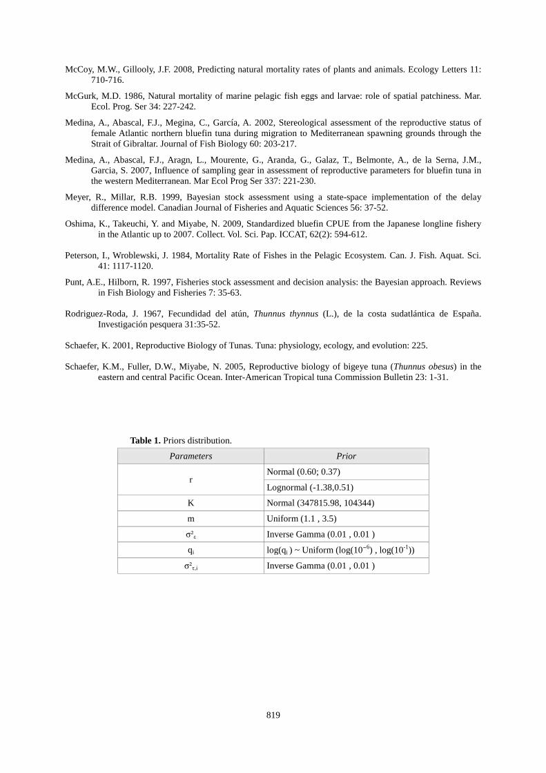
). Priors are reported in Table 1.

Shape parameter We used for m a uniform prior with 1.1 as lower bound and 3.5 upper bound. Because, m>2 makes little (unclear) sense, we also constrained this parameter to be equal to: m=1.1, m=1.5 and m=2 within 3 scenarios. Carrying capacity Prior distribution for carrying capacity was simply assumed to follow a Gaussian distribution with mean equal to the maximum biomass estimated by VPA with 30% of CV. This corresponds to the estimated biomass in 1958 of 347816 tons (with a SSB of 323776 tons). Intrinsic population growth rate To build an informative prior of r, we used a demographic approach proposed by Mc Allister et al (2001). We chose to work with Leslie matrix model. This model is based on two equations: − The survival equation 𝑁𝑖+1,𝑡+1 = 𝑁𝑖,𝑡 . 𝑆𝑖Ni, t is the number of age i individuals at time t, and Si the

survival rate from age i to age i+1. − The reproduction equation 𝑁0,𝑡+1 = � 𝑁𝑖,𝑡

𝐴𝑖=0 .𝑚𝑖 the number of age 0 individuals depends on mi

: average number of age zero individuals produced by an individual of age i.

As matrix form, the model is written[𝑁𝑖]𝑡+1 = 𝐿. [𝑁𝑖]𝑡with [Ni] t

�

𝑚0 𝑚𝑖 𝑚𝐴 0𝑆0 0 . . . 00 𝑆𝑖 . . 00 0 𝑆𝐴 0

�

is the vector of numbers of individuals in age group i at time t and L is the Leslie matrix of the form:

814

This matrix is constant over time, we can write: [𝑁𝑖]𝑡+𝑛 = 𝐿𝑛 . [𝑁𝑖]𝑡. The matrix coefficients are all positive, it can be shown the rate of population growth is 𝑟 = ln(𝜆), with λ the first eigen value of matrix L. From the first eigen value computed for 20000 Leslie population matrices, we obtained an empirical distribution of the intrinsic growth rate of the population and a probability density function is fitted. To do so, available information in the literature on various parameters of reproductive biology and life history traits of bluefin tuna was collected to perform the probability distribution functions (pdf) of each parameter of interest, taking into account knowledge and uncertainties on their distributions (Table 2). 20000 vectors were randomly drawn to calculate the different components of Leslie population matrices, i.e., annual survival rate at age i Si (age 1 to age 35), survival of age 0 S0 (young-of the year), and expected number of female produced per spawner mi

, respectively.

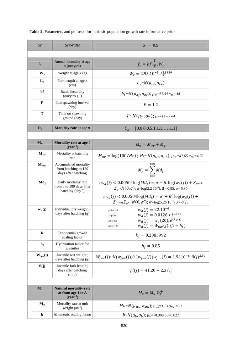
Expected number of female produced per spawner mx is the mean number of age 0 female (eggs) produced per a age-x female. It is the product of the sex-ratio sr, the annual fecundity fx, and the rate of mature female at age x Ox

𝑚𝑥 = 𝑠𝑟. 𝑓𝑥.𝑂𝑥

:

Sex-ratio We considered sr = 0.5 Annual fecundity fx

is the annual fecundity in number of oocytes per year

𝑓𝑥 = 𝑁𝑏 . bf.𝑊𝑥 =𝑇𝐼𝑖

. bf.𝑊𝑥

Nb is the number of batches per year which is deduced from the time spent on a spawning ground T and the time interval between 2 batch Ii. bf is the relative batch fecundity (i.e. the number of oocytes expelled per grammes of body. Wx

is the mean weight of an age-x female during spawning.

Spawning periodicity: Archival tagging reveals various migratory patterns, with matures individuals absent of spawning ground during reproductive events (Galuardi et al. 2010; (Fromentin et Powers 2005). In addition to that, non stimulated spawning cannot be obtained in captivity Lioka et al. (2000) We tested 3 hypothesis for spawning periodicity: every year, every 2 years and every 3 years by dividing the total fecundity by 2 or 3. Relative batch fecundity: We examined previous studies and data on the fecundity of bluefin and other tunas: (Rodriguez-Roda 1967) (Baglin 1976) (Schaefer 2001) (Farley et Davis 1998), (Schaefer et al. 2005) (Medina et al. 2002) (Itano 2000) (Medina et al. 2007). After interactions with fish biologists, we finally retained the most recent works of Medina et al (2002 and 2007). We used values of batch fecundity given in these studies for 2 samples (n=24 and n=48). A Gaussian distribution N(μbf, σbf ) is fitted, we obtained μbf,=61.44 and σbf

=48

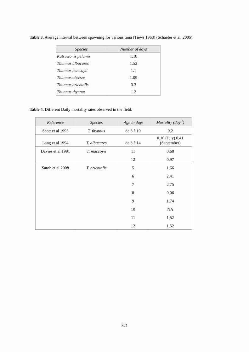
Spawning frequency: Spawning frequency is generally estimated from the observation of post-ovulatory follicles. Despite uncertainties on the length of the regression period, one can deduced the inter-spawning interval from the number of mature females presenting this type of follicles. Table 3 provides estimation of inter-spawning interval for 6 species of tunas. For bluefin this period is probably around 1.2 (Medina et al. 2007). Duration of spawning process: Direct observations throw archival tagging tend to reveal that a spawner may stay for 2 weeks on a spawning ground (Block and Stevens 2001). We then considered a reasonable value of 14 days with 90% of probability that this value stays between 7 and 21. This correspond approximately to a normal probability function N(μT, σT ) with μT = 14 et σT

= 4

Length growth and length-weight conversion factors Because the growth curve proposed by Restrepo et al (2009) is very close to this of Cort (1991) and because we wanted weight-at-age for fish > 20 yrs, we used the mean length at age and standard deviation predicted by Restrepo et al. (2009). Values drawn from those distributions are converted in weight with the conversion factors used for East Atlantic bluefin.

815

𝑊𝑥 = 2.95. 10−5.𝐿𝑥2.8989 ; 𝐿𝑥~𝑁(𝜇𝑥 ,𝜎𝑥)

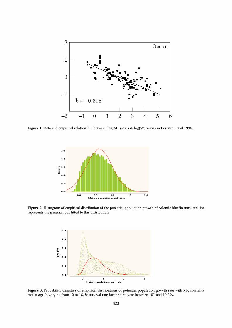
Maturity rate Histological observation of ovaries associated with the count of translucent zones on the ray of the first dorsal fin showed that median sexual maturity is reached at 103.6 cm FL. (see Corriero et al. 2003 based on a sample of 501 BFT females from the western and central Mediterranean). We considered for our study that half of the females are mature at 4 years-old and that there are all spawner after. Survival rates and natural mortalities Natural mortalities after the first year Various works investigated some empirical relationships between natural mortalities of adults/ juveniles and growth in length/weight (see McGurk 1986) (Lorenzen 1996), (Andersen et Beyer 2006) (McCoy et Gillooly 2008) (Gislason et al. 2008). We choose to refer to the simple relationship proposed by Lorenzen et al (1996) (Figure 1).

𝑀𝑊 = 𝑀𝑢𝑊𝑏 MW is the natural mortality rate at weight W, Mu

is the natural mortality per unit of weight and b is the allometric scaling factor. This relationship has been adjusted to data concerning 269 fish populations (adults and juveniles) frequenting temperate ecosystems.

Natural mortality during the first year Mortality process operating from fecundation to the end of the first year is known to be very high and to mostly determine the recruitment success of a given cohort (e.g. Hjort 1926). We worked specifically on a distribution for mortality/survival rate of young-of the year. We considered that the age 0 corresponds to the first six months of live (from birth to end of December). The mortality rate M0 is the sum of two terms: MHr, mortality rate due to hatching rate and My.

𝑀0 = 𝑀𝐻𝑟 + 𝑀𝑦

mortality of the early stages (larvae and then juveniles).

Hatching rate: For Thunnus thynnus, (Lioka et al. 2000) indicate hatching rates of 83.3% and 88.2%, with respectively 57% and 38.3% qualified as “normal hatching”. (Margulies et al. 2007) observed a mean hatching rate of 83% (standard deviation 14.7%) on Thunnus albacares but did not give information about larvae viability. We retained Lioka et al. results and proposed to considerer that Hr have a Gaussian distribution with mean μHr = 47.65 and a coefficient of variation of 10%. MHr

is given by:

𝑀𝐻𝑟 = log �100𝐻𝑟�, with 𝐻𝑟~𝑁(𝜇𝐻𝑟,0.1𝜇𝐻𝑟)

Daily mortality rate of larvae: Total mortality between hatching and the end of age 0 is split into daily mortality rate Mdx. In the same way as the mortality rate of adult, an empirical relationship was established between the daily mortality rate of larvae and their dry weight wd

(Peterson et Wroblewski 1984) (McGurk 1986).

𝑀𝑑 = 2.210−4𝑤𝑑−0.855 10-5 g <wd< 7 10-3

𝑀𝑑 = 5.2610−3𝑤𝑑−0.251.9 g <w g

d <1,4 10'4

g

We used these relationships to predict an "average" daily mortality of the larvae and juveniles from hatching until 180 days after hatching. To estimate the variance around the average mortality rate, we applied (Mangel et al. 2009) relationships on McGurk's data, i.e.:

log(𝑀𝑑𝑥) = 𝛼 + 𝛽. log(𝑤𝑑(𝑥)) + 𝑍𝜎with 𝑍𝜎~𝑁(0,𝜎)for wd

log(𝑀𝑑𝑥) = 𝛼′ + 𝛽′. log(𝑤𝑑(𝑥)) + 𝑍𝜎′with𝑍𝜎′~𝑁(0,𝜎′)for w< 0.00504 g

d

> 0.00504 g

The cumulated mortality upon this period is: 𝑀𝑦 = ∑ 𝑀𝑑𝑥180𝑥=0

816

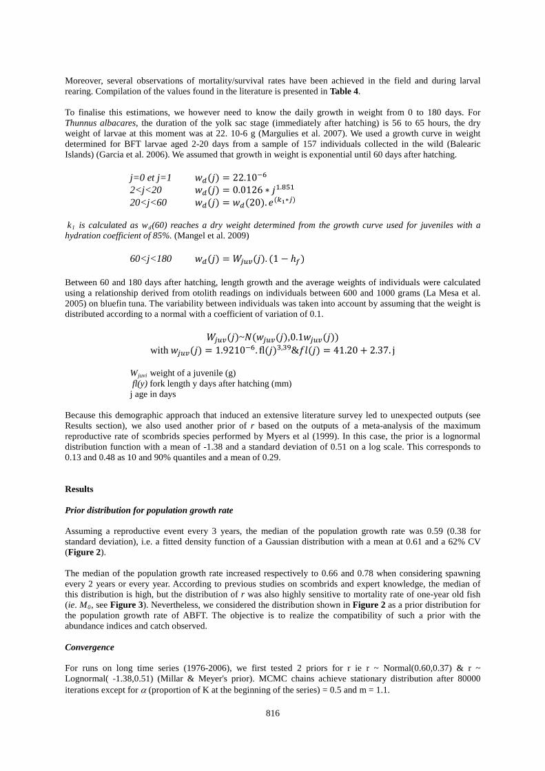
Moreover, several observations of mortality/survival rates have been achieved in the field and during larval rearing. Compilation of the values found in the literature is presented in Table 4. To finalise this estimations, we however need to know the daily growth in weight from 0 to 180 days. For Thunnus albacares, the duration of the yolk sac stage (immediately after hatching) is 56 to 65 hours, the dry weight of larvae at this moment was at 22. 10-6 g (Margulies et al. 2007). We used a growth curve in weight determined for BFT larvae aged 2-20 days from a sample of 157 individuals collected in the wild (Balearic Islands) (Garcia et al. 2006). We assumed that growth in weight is exponential until 60 days after hatching. j=0 et j=1 𝑤𝑑(𝑗) = 22.10−6 2<j<20 𝑤𝑑(𝑗) = 0.0126 ∗ 𝑗1.851 20<j<60 𝑤𝑑(𝑗) = 𝑤𝑑(20). 𝑒(𝑘1∗𝑗) k1 is calculated as wd

(60) reaches a dry weight determined from the growth curve used for juveniles with a hydration coefficient of 85%. (Mangel et al. 2009)

60<j<180 𝑤𝑑(𝑗) = 𝑊𝑗𝑢𝑣(𝑗). (1 − ℎ𝑓) Between 60 and 180 days after hatching, length growth and the average weights of individuals were calculated using a relationship derived from otolith readings on individuals between 600 and 1000 grams (La Mesa et al. 2005) on bluefin tuna. The variability between individuals was taken into account by assuming that the weight is distributed according to a normal with a coefficient of variation of 0.1.

𝑊𝑗𝑢𝑣(𝑗)~𝑁(𝑤𝑗𝑢𝑣(𝑗),0.1𝑤𝑗𝑢𝑣(𝑗)) with 𝑤𝑗𝑢𝑣(𝑗) = 1.9210−6. �l(𝑗)3,39&𝑓𝑙(𝑗) = 41.20 + 2.37. j

Wjuvi fl(y) fork length y days after hatching (mm)

weight of a juvenile (g)

j age in days Because this demographic approach that induced an extensive literature survey led to unexpected outputs (see Results section), we also used another prior of r based on the outputs of a meta-analysis of the maximum reproductive rate of scombrids species performed by Myers et al (1999). In this case, the prior is a lognormal distribution function with a mean of -1.38 and a standard deviation of 0.51 on a log scale. This corresponds to 0.13 and 0.48 as 10 and 90% quantiles and a mean of 0.29. Results Prior distribution for population growth rate Assuming a reproductive event every 3 years, the median of the population growth rate was 0.59 (0.38 for standard deviation), i.e. a fitted density function of a Gaussian distribution with a mean at 0.61 and a 62% CV (Figure 2). The median of the population growth rate increased respectively to 0.66 and 0.78 when considering spawning every 2 years or every year. According to previous studies on scombrids and expert knowledge, the median of this distribution is high, but the distribution of r was also highly sensitive to mortality rate of one-year old fish (ie. M0

, see Figure 3). Nevertheless, we considered the distribution shown in Figure 2 as a prior distribution for the population growth rate of ABFT. The objective is to realize the compatibility of such a prior with the abundance indices and catch observed.

Convergence For runs on long time series (1976-2006), we first tested 2 priors for r ie r ~ Normal(0.60,0.37) & r ~ Lognormal( -1.38,0.51) (Millar & Meyer's prior). MCMC chains achieve stationary distribution after 80000 iterations except for α (proportion of K at the beginning of the series) = 0.5 and m = 1.1.

817

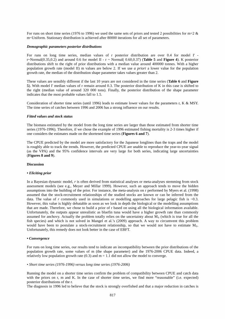
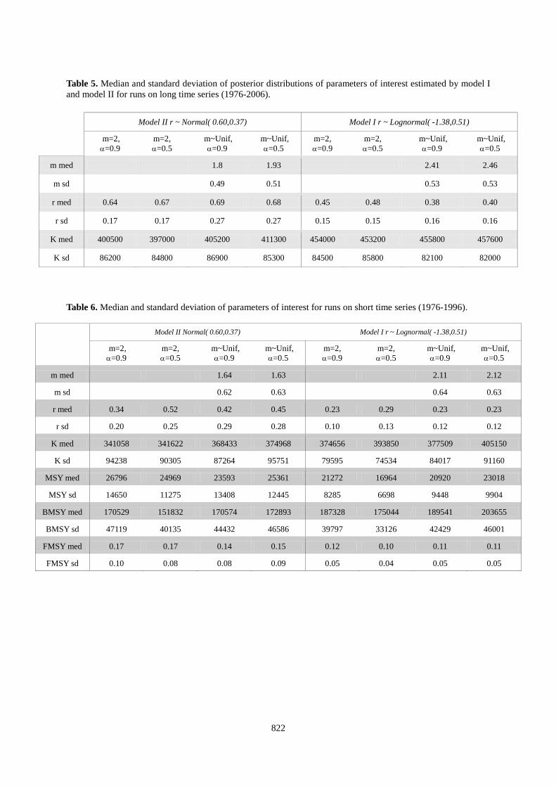
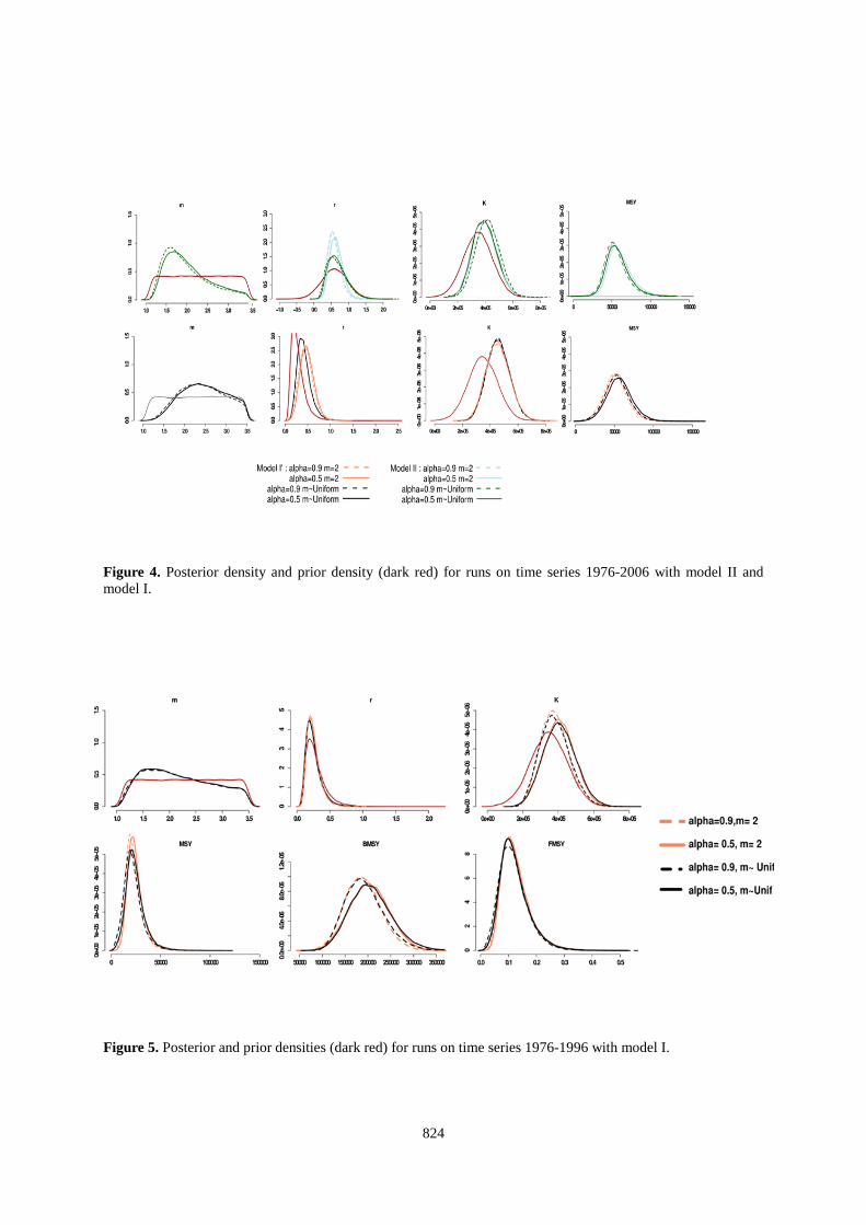
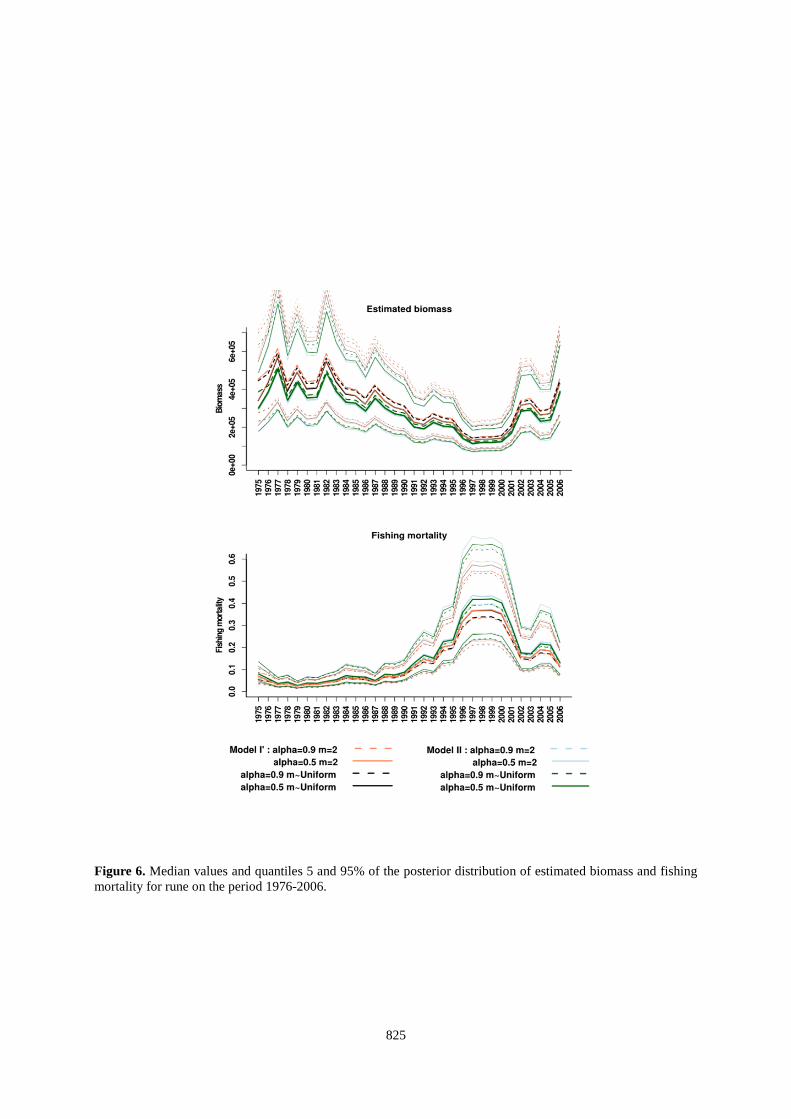
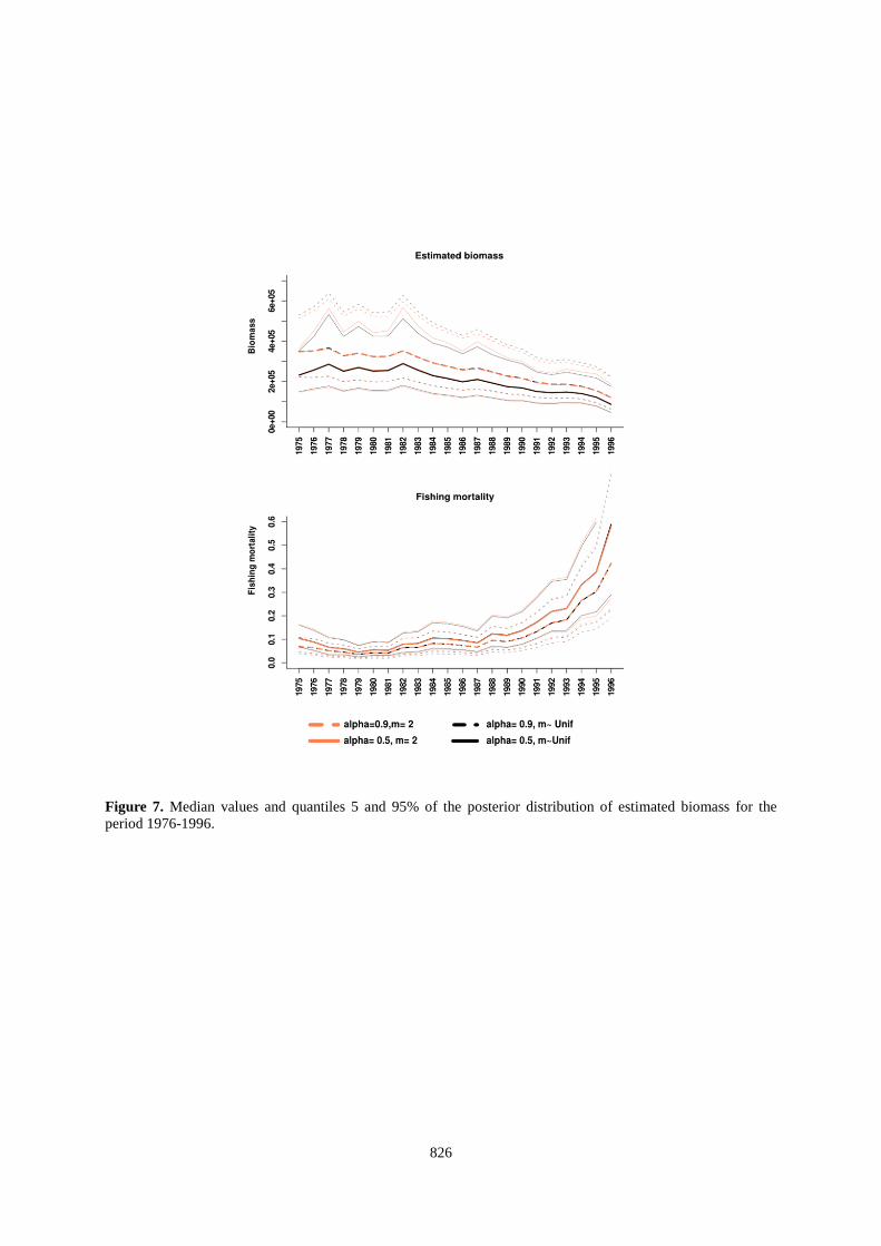
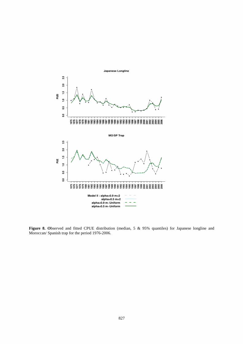
For runs on short time series (1976 to 1996) we used the same sets of priors and tested 2 possibilities for m=2 & m~Uniform. Stationary distribution is achieved after 80000 iterations for all set of parameters. Demographic parameters posterior distributions For runs on long time series, median values of r posterior distribution are over 0.4 for model I' - r~Normal(0.35,0.2) and around 0.6 for model II - r ~ Normal( 0.60,0.37) (Table 5 and Figure 4). K posterior distributions shift to the right of prior distributions with a median value around 400000 tonnes. With a higher population growth rate (model II) m values are below 2. If we use a priori a lower value for the population growth rate, the median of the distribution shape parameter takes values greater than 2. These values are sensibly different if the last 10 years are not considered in the time series (Table 6 and Figure 5). With model I' median values of r remain around 0.3. The posterior distribution of K in this case is shifted to the right (median value of around 320 000 tons). Finally, the posterior distribution of the shape parameter indicates that the most probable values fall to 1.5. Consideration of shorter time series (until 1996) leads to estimate lower values for the parameters r, K & MSY. The time series of catches between 1996 and 2006 has a strong influence on our results. Fitted values and stock status The biomass estimated by the model from the long time series are larger than those estimated from shorter time series (1976-1996). Therefore, if we chose the example of 1996 estimated fishing mortality is 2-3 times higher if one considers the estimates made on the shortened time series (Figures 6 and 7). The CPUE predicted by the model are more satisfactory for the Japanese longlines than the traps and the model is roughly able to track the trends. However, the predicted CPUE are unable to reproduce the year-to-year signal (as the VPA) and the 95% confidence intervals are very large for both series, indicating large uncertainties (Figures 8 and 9). Discussion • Eliciting prior In a Bayesian dynamic model, r is often derived from statistical analyses or meta-analyses stemming from stock assessment models (see e.g., Meyer and Millar 1999). However, such an approach tends to move the hidden assumptions into the building of the prior. For instance, the meta-analysis on r performed by Myers et al. (1998) assumed that the stock-recruitment relationships of the studied stocks are known or can be inferred from the data. The value of r commonly used in simulations or modelling approaches for large pelagic fish is ~0.3. However, this value is highly debatable as soon as we look in depth the biological or the modelling assumptions that are made. Therefore, we chose to build a prior of r based on using all the biological information available. Unfortunately, the outputs appear unrealistic as bluefin tuna would have a higher growth rate than commonly assumed for anchovy. Actually the problem totally relies on the uncertainty about M0 (which is true for all the fish species) and which is not solved in Mangel et al.’s (2009) approach. A way to circumvent this problem would have been to postulate a stock-recruitment relationship, so that we would not have to estimate M0

. Unfortunately, this remedy does not look better in the case of EBFT.

• Convergence For runs on long time series, our results tend to indicate an incompatibility between the prior distributions of the population growth rate, some values of m (the shape parameter) and the 1976-2006 CPUE data. Indeed, a relatively low population growth rate (0.3) and m = 1.1 did not allow the model to converge. • Short time series (1976-1996) versus long time series (1976-2006) Running the model on a shorter time series confirm the problem of compatibility between CPUE and catch data with the priors on r, m and K. In the case of shorter time series, we find more “reasonable” (i.e. expected) posterior distributions of the r. The diagnosis in 1996 led to believe that the stock is strongly overfished and that a major reduction in catches is

818

needed. However, this is in contradiction with the high catch levels between 1996 and 2006 (between 30,000 tonnes to 40,000 for non-inflated catch and between 40,000 and 50,000 tonnes for inflated catch) because, as we said, this parametrisation of the biomass dynamic model cannot handle this high catch volume. The only way of the model to deal with these catches is to estimate large values of r and K (and thus high BMSY

), probably because the CPUE series did not display any strong contrast. Although these gears target approximately the same age classes, their signals are not similar and this probably makes problem for the estimation of the parameters of the biomass dynamics models. The traps catch tuna during their migration while the long-line target a mix of individuals (i.e., potentially migratory and resident individuals in feeding areas). It is also not excluded that the standardization of CPUE traps should involve oceanographic conditions that may affect the migration routes of tuna to reflect the size of the migrant stock.

References Andersen, K.H., Beyer, J.E. 2006, Asymptotic Size Determines Species Abundance in the Marine Size Spectrum.

The American Naturalist 168: 54-61.

Baglin, R.E. 1976, A preliminary study of the gonadal development and fecundity of the western Atlantic bluefin tuna. Collect. Vol. Sci. Pap. ICCAT, 5: 279-289.

Block, B.A., Stevens, E.D. 2001, Tuna: physiology, ecology, and evolution. Academic Pr.

Corriero, A., Desantis, S., Deflorio, M., Acone, F., Bridges, C.R., de la Serna, J.M., Megalofonou, P., Metrio, G.D. 2003, Histological investigation on the ovarian cycle of the bluefin tuna in the western and central Mediterranean. Journal of Fish Biology 63: 108-119.

Farley. J.H., Davis, T.L. 1998, Reproductive dynamics of southern bluefin tuna, Thunnus maccoyii. Fishery Bulletin 96: 223-236.

Fromentin, J., Powers, J.E. 2005, Atlantic bluefin tuna: population dynamics, ecology, fisheries and management. Fish and Fisheries 6: 281-306.

Garcia, A., Cortés, D., Ramırez, T., Fehri-Bedoui, R., Alemany, F., Rodrıguez, J.M., Carpena, Á., Álvarez, J.P. 2006, First data on growth and nucleic acid and protein content of field-captured Mediterranean bluefin (Thunnus thynnus) and albacore (Thunnus alalunga) tuna larvae: a comparative study. Scientia Marina 70.

Gislason, H., Pope, J.G., Rice, J.C., Daan, N. 2008, Coexistence in North Sea fish communities: Implications for growth and natural mortality. ICES J. Mar. Sci. 65: 514-530.

Itano, D.G. 2000, The reproductive biology of yellowfin tuna (Thunnus albacares) in Hawaiian waters and the western tropical Pacific Ocean: Project summary. SOEST 00-01 JIMAR Contribution 00-328. Pelagic Fisheries Research Program, JIMAR, University of Hawaii.

ICCAT. 2005, Report of the 2004 Data Exploratory Meeting for the East Atlantic and Mediterranean Bluefin Tuna. Collect. Vol. Sci. Pap. ICCAT, 58(2): 662-699.

ICCAT. 2009, Report of the 2008 Atlantic Bluefin Tuna Stock Assessment Session. Collect. Vol. Sci. Pap. ICCAT 64(1): 1-352.

La Mesa, M., Sinopoli, M., Andaloro, F. 2005, Age and growth rate of juvenile bluefin tuna Thunnus thynnus from the Mediterranean Sea (Sicily, Italy). Scientia Marina 69.

Lioka, C., Kani, K., Nhhala, H. 2000, Present status and prospects of technical developmment of tuna sea-farming. Cahiers Option Mediterraneennes, 47: 275-285.

Lorenzen, K. 1996, The relationship between body weight and natural mortality in juvenile and adult fish: a comparison of natural ecosystems and aquaculture. Journal of Fish Biology 49: 627-647.

Mangel, M., Brodziak, J., DiNardo, G. 2009, Reproductive ecology and scientific inference of steepness: a fundamental metric of population dynamics and strategic fisheries management. Fish and Fisheries 9999.

Margulies, D., Suter, J.M., Hunt, S.L., Olson, R.J., Scholey, V.P., Wexler, J.B., Nakazawa, A. 2007, Spawning and early development of captive yellowfin tuna (Thunnus albacares). Fishery Bulletin-National Oceanic and Atmospheric Administration 105:249.

McAllister, M.K., Pikitch, E.K., Babcock, E.A. 2001, Using demographic methods to construct Bayesian priors for the intrinsic rate of increase in the Schaefer model and implications for stock rebuilding. Canadian Journal of Fisheries and Aquatic Sciences 58: 1871-1890.

819

McCoy, M.W., Gillooly, J.F. 2008, Predicting natural mortality rates of plants and animals. Ecology Letters 11: 710-716.

McGurk, M.D. 1986, Natural mortality of marine pelagic fish eggs and larvae: role of spatial patchiness. Mar. Ecol. Prog. Ser 34: 227-242.

Medina, A., Abascal, F.J., Megina, C., García, A. 2002, Stereological assessment of the reproductive status of female Atlantic northern bluefin tuna during migration to Mediterranean spawning grounds through the Strait of Gibraltar. Journal of Fish Biology 60: 203-217.

Medina, A., Abascal, F.J., Aragn, L., Mourente, G., Aranda, G., Galaz, T., Belmonte, A., de la Serna, J.M., Garcia, S. 2007, Influence of sampling gear in assessment of reproductive parameters for bluefin tuna in the western Mediterranean. Mar Ecol Prog Ser 337: 221-230.

Meyer, R., Millar, R.B. 1999, Bayesian stock assessment using a state-space implementation of the delay difference model. Canadian Journal of Fisheries and Aquatic Sciences 56: 37-52.

Oshima, K., Takeuchi, Y. and Miyabe, N. 2009, Standardized bluefin CPUE from the Japanese longline fishery in the Atlantic up to 2007. Collect. Vol. Sci. Pap. ICCAT, 62(2): 594-612.

Peterson, I., Wroblewski, J. 1984, Mortality Rate of Fishes in the Pelagic Ecosystem. Can. J. Fish. Aquat. Sci.

41: 1117-1120.

Punt, A.E., Hilborn, R. 1997, Fisheries stock assessment and decision analysis: the Bayesian approach. Reviews in Fish Biology and Fisheries 7: 35-63.

Rodriguez-Roda, J. 1967, Fecundidad del atún, Thunnus thynnus (L.), de la costa sudatlántica de España.

Investigación pesquera 31:35-52. Schaefer, K. 2001, Reproductive Biology of Tunas. Tuna: physiology, ecology, and evolution: 225. Schaefer, K.M., Fuller, D.W., Miyabe, N. 2005, Reproductive biology of bigeye tuna (Thunnus obesus) in the

eastern and central Pacific Ocean. Inter-American Tropical tuna Commission Bulletin 23: 1-31.

Table 1. Priors distribution.

Parameters Prior

r Normal (0.60; 0.37)

Lognormal (-1.38,0.51)

K Normal (347815.98, 104344)

m Uniform (1.1 , 3.5)

σ²ε Inverse Gamma (0.01 , 0.01 )

qi log(qi ) ~ Uniform (log(10⁻6) , log(10-1))

σ²τ,i Inverse Gamma (0.01 , 0.01 )

820

Table 2. Parameters and pdf used for intrinsic population growth rate informative prior.

Sr Sex-ratio 𝑆𝑟 = 0.5

f Annual fecundity at age x (oocytes) x 𝑓𝑥 = 𝑏𝑓.

𝑇𝐹

.𝑊𝑥

W Weight at age x (g) x 𝑊𝑥 = 2.95.10−5.𝐿𝑥2.8989

L Fork length at age x (cm)

x 𝐿𝑥~𝑁(𝜇𝐿𝑥 ,𝜎𝐿𝑥)

bf Batch fecundity (oocytes.g-1 𝑏𝑓~𝑁(𝜇𝑏𝑓,𝜎𝑏𝑓); μ) bf=61.44 σbf,

F

=48

Interspawning interval (day) 𝐹 = 1.2

T Time on spawning ground (day) 𝑇~𝑁(𝜇𝑇 ,𝜎𝑇); μT=14 σT,

=4

O Maturity rate at age x x 𝑂𝑥 = [0,0,0,0.5,1,1,1, . . . .1,1]

M Mortality rate at age 0 (year

0 -1 𝑀0 = 𝑀𝐻𝑟 + 𝑀𝑦 )

M Mortality at hatching rate

Hr 𝑀𝐻𝑟 = log(100 𝐻𝑟⁄ ) ; 𝐻𝑟~𝑁(𝜇𝐻𝑟 ,𝜎𝐻𝑟); μHr=47.65 σHr,

=4.76

M Accumulated mortality from hatching to 180 days after hatching

larv 𝑀𝑦 = �𝑀𝑑𝑗

180

𝑗=0

Md Daily mortality rate from 0 to 180 days after

hatching (day

j

-1

if 𝑤𝑑(𝑗) < 0.00504log(𝑀𝑑𝑗) = 𝛼 + 𝛽. log(𝑤𝑑(𝑗)) + 𝑍𝜎with

𝑍𝜎~𝑁(0,𝜎); α=log(2.2 10) -4

), β=-0.85, σ= 0.80

if 𝑤𝑑(𝑗) < 0.00504log(𝑀𝑑𝑗) = 𝛼′ + 𝛽′. log(𝑤𝑑(𝑗)) +𝑍𝜎′with𝑍𝜎′~𝑁(0,𝜎′); α'=log(5.26 10-3

) β'=-0.25

wd Individual dry weight j days after hatching (g)

(j) j=0 et j=1 𝑤𝑑(𝑗) = 22.10−6

2<j<20 𝑤𝑑(𝑗) = 0.0126 ∗ 𝑗1.851

20<j<60 𝑤𝑑(𝑗) = 𝑤𝑑(20).𝑒(𝑘1∗𝑗)

61<j<180 𝑤𝑑(𝑗) = 𝑊𝑗𝑢𝑣(𝑗). (1− ℎ𝑓)

k Exponential growth scaling factor 𝑘1 = 0.2085992

h Hydratation factor for juveniles

f ℎ𝑓 = 0.85

Wjuv Juvenile wet weight j days after hatching (g)

(j) 𝑊𝑗𝑢𝑣(𝑗)~𝑁(𝑤𝑗𝑢𝑣(𝑗),0.1𝑤𝑗𝑢𝑣(𝑗))𝑤𝑗𝑢𝑣(𝑗) = 1.9210−6. �l(𝑗)3,39

fl(j) Juvenile fork length j days after hatching

(mm) 𝑓𝑙(𝑗) = 41.20 + 2.37. j

M Natural mortality rate

at from age 1 to A (year

x

-1𝑀𝑥 = 𝑀𝑢.𝑊𝑥

𝑏 )

M Mortality rate at unit weight (an

u -1 𝑀𝑢~𝑁(𝜇𝑀𝑢,𝜎𝑀𝑢); μ) mu=3.13 σMu,

b

=0.2

Allometric scaling factor 𝑏~𝑁(𝜇𝑏,𝜎𝑏); μb= -0.309 σb=0.027

821

Table 3. Average interval between spawning for various tuna (Tiews 1963) (Schaefer et al. 2005).

Species Number of days

Katsuwonis pelamis 1.18

Thunnus albacares 1.52

Thunnus maccoyii 1.1

Thunnus obsesus 1.09

Thunnus orientalis 3.3

Thunnus thynnus 1.2 Table 4. Different Daily mortality rates observed in the field.

Reference Species Age in days Mortality (day-1

Scott et al 1993

)

T. thynnus de 3 à 10 0,2

Lang et al 1994 T. albacares de 3 à 14 0,16 (July) 0,41

(September)

Davies et al 1991 T. maccoyii 11 0,68

12 0,97

Satoh et al 2008 T. orientalis 5 1,66

6 2,41

7 2,75

8 0,06

9 1,74

10 NA

11 1,52

12 1,52

822

Table 5. Median and standard deviation of posterior distributions of parameters of interest estimated by model I and model II for runs on long time series (1976-2006).

Model II r ~ Normal( 0.60,0.37) Model I r ~ Lognormal( -1.38,0.51)

m=2, α=0.9

m=2, α=0.5

m~Unif, α=0.9

m~Unif, α=0.5

m=2, α=0.9

m=2, α=0.5

m~Unif, α=0.9

m~Unif, α=0.5

m med 1.8 1.93 2.41 2.46

m sd 0.49 0.51 0.53 0.53

r med 0.64 0.67 0.69 0.68 0.45 0.48 0.38 0.40

r sd 0.17 0.17 0.27 0.27 0.15 0.15 0.16 0.16

K med 400500 397000 405200 411300 454000 453200 455800 457600

K sd 86200 84800 86900 85300 84500 85800 82100 82000

Table 6. Median and standard deviation of parameters of interest for runs on short time series (1976-1996).

Model II Normal( 0.60,0.37) Model I r ~ Lognormal( -1.38,0.51)

m=2, α=0.9

m=2, α=0.5

m~Unif, α=0.9

m~Unif, α=0.5

m=2, α=0.9

m=2, α=0.5

m~Unif, α=0.9

m~Unif, α=0.5

m med 1.64 1.63 2.11 2.12

m sd 0.62 0.63 0.64 0.63

r med 0.34 0.52 0.42 0.45 0.23 0.29 0.23 0.23

r sd 0.20 0.25 0.29 0.28 0.10 0.13 0.12 0.12

K med 341058 341622 368433 374968 374656 393850 377509 405150

K sd 94238 90305 87264 95751 79595 74534 84017 91160

MSY med 26796 24969 23593 25361 21272 16964 20920 23018

MSY sd 14650 11275 13408 12445 8285 6698 9448 9904

BMSY med 170529 151832 170574 172893 187328 175044 189541 203655

BMSY sd 47119 40135 44432 46586 39797 33126 42429 46001

FMSY med 0.17 0.17 0.14 0.15 0.12 0.10 0.11 0.11

FMSY sd 0.10 0.08 0.08 0.09 0.05 0.04 0.05 0.05

823

Figure 1. Data and empirical relationship between log(M) y-axis & log(W) x-axis in Lorenzen et al 1996. Figure 2. Histogram of empirical distribution of the potential population growth of Atlantic bluefin tuna. red line represents the gaussian pdf fitted to this distribution. Figure 3. Probability densities of empirical distributions of potential population growth rate with M0, mortality rate at age 0, varying from 10 to 16, ie survival rate for the first year between 10-3 and 10-5 %.

824

Figure 4. Posterior density and prior density (dark red) for runs on time series 1976-2006 with model II and model I. Figure 5. Posterior and prior densities (dark red) for runs on time series 1976-1996 with model I.

825

Figure 6. Median values and quantiles 5 and 95% of the posterior distribution of estimated biomass and fishing mortality for rune on the period 1976-2006.

826

Figure 7. Median values and quantiles 5 and 95% of the posterior distribution of estimated biomass for the period 1976-1996.

827

Figure 8. Observed and fitted CPUE distribution (median, 5 & 95% quantiles) for Japanese longline and Moroccan/ Spanish trap for the period 1976-2006.

828

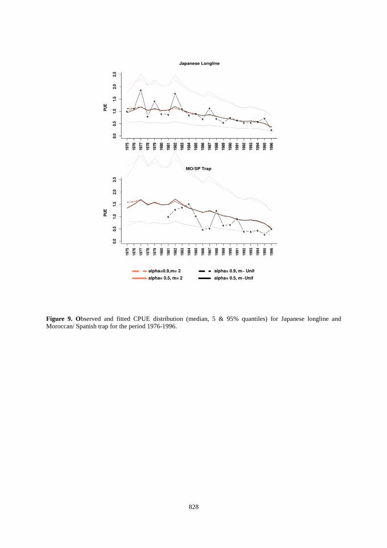
Figure 9. Observed and fitted CPUE distribution (median, 5 & 95% quantiles) for Japanese longline and Moroccan/ Spanish trap for the period 1976-1996.