Learning Priors for Bayesian Computations in theNervous SystemMax Berniker1*, Martin Voss2, Konrad Kording1

1 Department of Physical Medicine and Rehabilitation, Northwestern University and Rehabilitation Institute of Chicago, Chicago, Illinois, United States of America,

2 Department of Psychiatry and Psychotherapy, Charite University Hospital & St. Hedwig Hospital, Berlin, Germany

Abstract

Our nervous system continuously combines new information from our senses with information it has acquired throughoutlife. Numerous studies have found that human subjects manage this by integrating their observations with their previousexperience (priors) in a way that is close to the statistical optimum. However, little is known about the way the nervoussystem acquires or learns priors. Here we present results from experiments where the underlying distribution of targetlocations in an estimation task was switched, manipulating the prior subjects should use. Our experimental design allowedus to measure a subject’s evolving prior while they learned. We confirm that through extensive practice subjects learn thecorrect prior for the task. We found that subjects can rapidly learn the mean of a new prior while the variance is learnedmore slowly and with a variable learning rate. In addition, we found that a Bayesian inference model could predict the timecourse of the observed learning while offering an intuitive explanation for the findings. The evidence suggests the nervoussystem continuously updates its priors to enable efficient behavior.

Citation: Berniker M, Voss M, Kording K (2010) Learning Priors for Bayesian Computations in the Nervous System. PLoS ONE 5(9): e12686. doi:10.1371/journal.pone.0012686

Editor: Vladimir Brezina, Mount Sinai School of Medicine, United States of America

Received May 14, 2010; Accepted July 28, 2010; Published September 10, 2010

Copyright: � 2010 Berniker et al. This is an open-access article distributed under the terms of the Creative Commons Attribution License, which permitsunrestricted use, distribution, and reproduction in any medium, provided the original author and source are credited.

Funding: NIH grant nrs. 1R01NS063399 and 5P01NS0044393. The funders had no role in study design, data collection and analysis, decision to publish, orpreparation of the manuscript.

Competing Interests: The authors have declared that no competing interests exist.

* E-mail: mbernike@northwestern.edu

Introduction

For any sensorimotor behavior, we rely on our sensory inputs as

well as knowledge we have accumulated over the course of our life.

For example, when descending stairs we use our visually perceived

assessment of stair width and depth, but also our experience of

these typical attributes (as is evident when we descend stairs

without looking). Bayesian statistics provides a way of calculating

how prior knowledge can be combined with new information from

our senses in a statistically optimal way. A wide range of studies

has found that human behavior is close to these predictions of

optimal combination. In particular, the Bayesian use of prior

information has been observed in tasks such as the perception of

visual movement [1,2], cue combination [3,4], visuomotor

integration [5,6] movement planning [7] and motor adaptation

[8]. While these studies have shown that human subjects can

efficiently use prior information, little is known about the way such

priors are learned.

Based on experimental evidence (e.g., [9,10]) it is clear priors

can change, however, it is unclear how these priors change over

time, if they converge to the veridical distribution, and over what

time scales they change. We began our study with two hypotheses

concerning learning rates. It could be the case that both the mean

and the variance of a prior are learned at the same rate (see

Fig. 1A), perhaps mediated by the same neural mechanisms.

Consistent with many computational models of learning (e.g.,

[11,12]) neural processes of adaptation could fix this rate.

Alternatively, learning the mean and variance may proceed at

different rates (Fig. 1A) possibly mediated by distinct neural

mechanisms. This would be consistent with statistical consider-

ations if the different variables have differing levels of uncertainty.

Similarly, recent evidence suggesting specific cortical regions

modulate learning rates [13] based on representations of

uncertainty [14,15] implies this type of learning may be the norm.

Our aim was to determine how human subjects learned a prior

and what strategy may have been responsible for it.

We designed three versions of a ‘‘coin catching’’ experiment to

examine if subjects could not only estimate a prior, but also

independently estimate both the mean and the variance of the

prior. In the first experiment we found evidence that subjects

eventually estimated an accurate prior, and the number of trials

necessary for this. In the second experiment we found that subjects

could learn the variance of a prior independent of their estimate of

the mean. In the third experiment we found evidence that subjects

could correctly estimate multiple means for a prior, and when to

switch between them. For comparison we examined multiple

Bayesian inference models and compared their performance on

the same tasks. This analysis offered an intuitive explanation for

the seeming changes in learning rates subjects exhibited as the

experiment progressed. In addition, we found that subjects were

able to infer a new mean in the prior nearly as quickly as a

Bayesian inference model. Taken together, we present strong

evidence that subjects are capable of acquiring an accurate prior,

with multiple and variable learning rates, and using it to make

statistically optimal decisions.

Methods

In a ‘‘coin catching’’ task we investigated how subjects adapted

their expectation of coin locations (a prior) in response to changes

PLoS ONE | www.plosone.org 1 September 2010 | Volume 5 | Issue 9 | e12686

in the underlying distribution. Subjects had to estimate the

location of a virtual target coin, randomly drawn from a normal

distribution. On every trial, subjects were given noisy information

of the coins current location, in the form of a single ‘‘cue coin’’

(similar to the experimental design of [10]) and were then asked to

guess the location of the ‘‘target coin’’. To successfully estimate the

target coin’s location, subjects needed to integrate the coin’s

likelihood (obtained from the cue coin) with its prior (the

distribution of previous target coin locations). By collecting data

on where the subjects estimated the target coin to be, we could

then estimate the prior used by the subject and analyze its

temporal evolution.

Experimental protocolAll experimental protocols were approved by the Northwestern

University Institutional Review Board and were in accordance

with Northwestern University’s policy statement on the use of

humans in experiments. All participants were naıve to the goals of

the experiment, signed consent forms and were paid to participate.

Subjects were seated in front of a computer screen and given an

electronic paddle wheel (Griffin PowerMate). On a computer

monitor a thin vertical bar the height of the screen was

superimposed above a natural lake setting. Subjects were shown

how to use the paddle wheel to control the location of the ‘‘net’’

(the thin bar) on the screen. A program created specifically for

these experiments (in Matlab) obtained the positions of the target

coin from a specified Gaussian distribution. This distribution was

the experiment’s prior. The target coin’s horizontal location was

then used as the mean of a second Gaussian distribution to

randomly draw the location of the cue coin. In each trial, this cue

coin was displayed first and only extinguished at the trials

conclusion. The subjects would then move the net to the location

they believed would most likely ‘‘catch’’ the target coin. Since the

net covered the entire height of the screen only the horizontal

location was relevant, rendering this a one-dimensional task. After

the paddle wheel was depressed the target coin was displayed, with

an indication of whether or not the subject had successfully

‘‘caught’’ it and what their running score was (Fig. 1B). Thus the

cue coin was noisy evidence of the target coin’s location: the

likelihood. The mean of this distribution was defined by the

location of the cue coin. Similarly, the variance of this distribution

was observed from trial to trial through the spread between cue

and target coin locations. To correctly estimate the target coin’s

location, subjects would have to integrate this likelihood with an

estimated prior over target coin locations. By remembering the

target coin’s location from trial to trial, subjects can infer this prior.

With slight variations (see below) subjects were instructed that an

individual standing behind them was tossing coins, two at a time.

These two coins left the individual’s hand at the same time, and flew

towards the lake. The first coin the subjects saw (the cue coin) landed

in the lake first, and they were to place the net where they were most

likely to catch the second (target) coin, currently in mid-flight and

about to land. They could take as much time as they needed. Once

they had appropriately placed the net and depressed the paddle wheel

they would find out if they caught the second coin. Additionally, they

were instructed that the individual was neither trying to help them

nor prevent them from catching the coins, and would not change the

way he tossed the coins in response to their behavior.

The target coin was caught if the net and the target coin

overlapped by at least 50% of the coins width. The screen units

were normalized between 20.5 (the left edge) and 0.5 (the right

edge). In each experiment the standard deviation of the likelihood

distribution’s was fixed at 0.1 (one tenth of the screen’s width). As

we were interested in the learning of priors, only their distributions

were manipulated (Fig. 1C). To ensure each subject inferred a

unique prior, a different random location centered at the middle of

the screen was used to define the prior’s mean for each subject

(drawn from a normal distribution with zero mean and a standard

deviation of 0.1). In the first experiment the prior’s variance was

one of two values, either 0.05 or 0.2. All subjects in experiment

one were given the instructions described above and asked to

perform 400 trials.

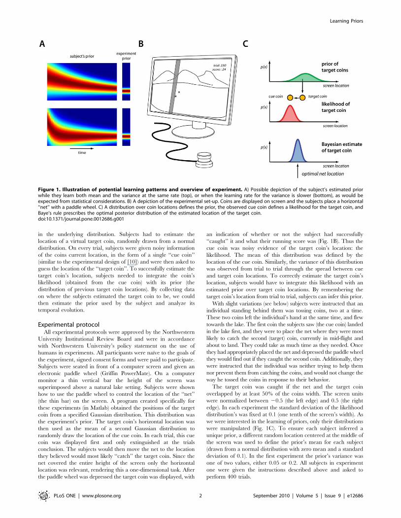
Figure 1. Illustration of potential learning patterns and overview of experiment. A) Possible depiction of the subject’s estimated priorwhile they learn both mean and the variance at the same rate (top), or when the learning rate for the variance is slower (bottom), as would beexpected from statistical considerations. B) A depiction of the experimental set-up. Coins are displayed on screen and the subjects place a horizontal‘‘net’’ with a paddle wheel. C) A distribution over coin locations defines the prior, the observed cue coin defines a likelihood for the target coin, andBaye’s rule prescribes the optimal posterior distribution of the estimated location of the target coin.doi:10.1371/journal.pone.0012686.g001

Learning Priors

PLoS ONE | www.plosone.org 2 September 2010 | Volume 5 | Issue 9 | e12686

In the second experiment subjects were given identical

instruction. Two values were used for the variance, the same

two values as used in experiment one (0.05 and 0.2). One of these

two values was randomly chosen at the start of the experiment and

assigned to the prior. After half of the trials (250) the prior’s

variance would switch to the other value. All subjects performed

500 trials in total after receiving the instructions described above.

In the third experiment two locations were used for the prior’s

mean, 20.05 and 0.05. After the completion of 10 trials, the

prior’s mean would flip to the other location based on a Bernoulli

probability of (p = 0.2). The prior’s variance was 0.1 throughout

the experiment. Subjects were given the instructions described

above, however, they were given the additional information that at

random times, the individual tossing the coins would move. All

subjects were asked to perform 600 Trials.

Data analysisIn order to perform the coin catching task successfully, in each

trial the net should be placed in the most likely location of the

target coin. According to Bayes’ rule, this is given as, mt = (12r)

mp+rml, where mp and ml are the mean of the prior, and the mean of

the likelihood (the cue coin’s location) and mt is the mean of the

target coin’s probability. r is defined through the variances of the

prior and likelihood (r = sp2/(sp

2+sl2)). In effect, r is an alternate

form of the Kalman gain. By recording the cue coin’s location, and

assuming the subjects placed the net where they believed the target

coin to be (mt), we can infer the parameter, r, and their belief of the

prior’s mean.

For all experiments, we wanted to examine both what subjects

learned (estimates of r and mp), as well as how these parameters

progressed across time. Therefore, for all subjects, each consec-

utive ten trials were binned together. This binned data was then

used to fit r and mp (in a linear least squares sense). Through this

procedure we obtained measures of how the subject’s estimates of

the prior developed in time. For experiment 3, we resorted the

data aligned to a switch in the prior’s mean and then binned all the

data in the subsequent 10 trials. Thus we could infer each subject’s

estimate of the prior’s mean, after a change in its value.

Bayesian inference analysisFor all the experiments, subjects would need to estimate the

prior’s mean and variance to successfully complete the trials. In

experiments 1 and 2, we wanted to examine how subjects adapted

their estimate of both the mean and the variance of the

experimental prior. Therefore, we designed a Bayesian inference

model to perform the same experiments (through simulation) and

to estimate both the mean and the variance of the experimental

prior. To simplify the analysis and make the model further

accurate, we assumed it accurately knew the likelihood’s variance.

The model’s performance was then used as a benchmark to

compare with the subjects. In experiment 3 every subject was

exposed to each of the two means for approximately 50 blocks of

trials during the course of the 600 trial experiments. Furthermore,

from the results of experiments 1 and 2 we concluded that subject’s

could estimate the prior’s mean relatively quickly. Based on this we

designed a Bayesian inference model that knew the prior’s correct

variance, but had to infer which of the two means was currently

being used. This model’s results were also compared with subject

behavior.

To analyze experiments 1 and 2 with our Bayesian approach we

need to propose probabilistic description of the prior’s mean and

variance. If the mean and variance were continuous and

unbounded variables then they could be represented with

Gaussian distributions and a Kalman filter could be used to

optimally estimate them. The prior’s mean can easily be modeled

in this manner. The variance, however, is only defined for positive

values and cannot be accurately described this way. Instead we

must limit ourselves to an appropriate non-negative distribution.

To do this we use the Normal-scaled Inverse Gamma (NIG)

distribution (see Appendix S1). There are multiple advantages to

using this representation. The NIG distribution is a conjugate prior

for a Gaussian likelihood, so we can easily update its parameter

values to compute a posterior distribution. Further, it correctly

limits the variance to non-negative values, and assigns vanishingly

small probabilities to a variance of zero.

For experiments 1 and 2 we used the NIG distribution to

examine the performance of a Bayesian inference model. The

model has four free parameters. For a given set of these

parameters, we could simulate many experiments to find the

model’s average estimates for, mp and sp2 and the resulting r. To

obtain a ‘best’ set of the four free parameters and avoid over-

fitting, we found the values that maximized the log likelihood of

observing the across subject average binned data, means, mp and

gains, r, from experiment’s 1A and 1B. With these parameter

values fixed, the Bayesian inference model was then used to

simulate many runs of experiment 2 to find the model’s average

performance. See Appendix S1 for more details. These results

could then be compared with the across subject average

performance. Finally, as a further point for comparison, we also

examined a linear model that only estimated the prior’s variance.

This model used a running window of the last ten trials to compute

a sample observation of the prior’s variance. The model then used

this observation to update its estimate of the variance using a fixed

learning rate; the model is essentially a linear filter (see Appendix

S1). Using these two models as a point of reference, we could

compare subjects’ performance with both a simple model, and a

Bayes’ optimal model of inference.

In experiment 3, during the course of the 600 trials of this

experiment, each subject was exposed to each of the two means for

approximately 50 blocks of trials. Based on this, and similar

considerations noted above, we assumed the inference model had

access to the true variance but had to infer which of the two means

was currently being used. For this analysis, the inference model

used the coins displayed on each trial to compute the probability

that either mean was currently in use, and the most likely target

location. In contrast with the previous Bayesian inference model,

there were no free parameters. As with the analysis of experiments

1 and 2, we simulated many identical versions of experiment 3

(each with 600 trials) to obtain the average model performance.

See Appendix S1 for more details.

Results

We designed an experiment where we monitor a subject’s prior

while they take part in a simple computerized game. In this game,

subjects are asked to try and catch coins with a net. On every trial

the subject is presented with noisy evidence of the coin’s location (a

cue coin). The subject then places a virtual net where they think

they are most likely to catch target coin. Subjects were instructed

to attempt to catch as many coins as possible. The locations of the

cue coin were drawn from a distribution centered on the target

coin. Thus the cue coin by itself provides the subject with evidence

of where the target coin will land, defining a likelihood. The

variance of this likelihood was held constant throughout all

experiments. The mean of this likelihood however, was drawn

from a precursor distribution, the prior. Therefore, to accurately

predict the location of the target coin on each trial, subjects would

need to estimate the prior and integrate this information with the

Learning Priors

PLoS ONE | www.plosone.org 3 September 2010 | Volume 5 | Issue 9 | e12686

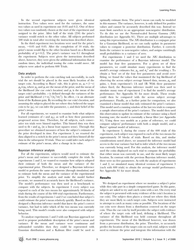
likelihood. In experiment 1 the prior was held constant, in

experiment 2 the variance of the prior changes and in a third

experiment the mean of the prior was changed periodically. As a

result, we could assess if subjects could estimate a prior, and if so,

whether they independently learned both the variance and mean

of this prior.

Experiment 1For each subject, one of two values, a large or small value, was

used to define the variance for that experiment’s prior. The mean

for the prior was chosen from a random location on the screen at

the start of each experiment. We found that given enough trials,

subjects tended to acquire a strategy that reflected an accurate

prior. For subjects exposed to the large variance (group 1A, N = 7),

cue and target coins appeared over relatively broad regions of the

screen. These subjects tended to choose net locations relatively

close to the displayed cue coin, as Bayesian integration would

prescribe (see Fig. 2). Similarly, for subjects exposed to the small

variance (group 1B, N = 7), cue and target coins appeared in a

relatively narrow region of the screen. These subjects tended to

choose net locations relatively close to the mean of the prior, again

consistent with Bayesian integration (see Fig. 2).

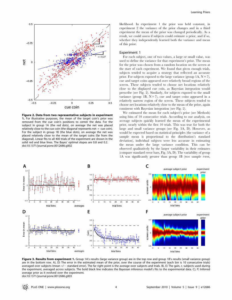
We estimated the mean for each subject’s prior (see Methods)

using bins of 10 consecutive trials. According to our analysis, on

average subjects quickly learned the mean of the experimental

prior, nearly within the first 10 trials. This was true for both the

large and small variance groups (see Fig. 3A, D). However, as

would be expected based on statistical principles (the variance of a

sample mean is proportional to the distribution’s standard

deviation), individual subjects were less accurate in estimating

the mean under the large variance condition. This can be

observed qualitatively by the larger variability in their estimates

(compare standard error bars, Fig. 3A, D). The variability of group

1A was significantly greater than group 1B (two sample t-test,

Figure 2. Data from two representative subjects in experiment1. For illustrative purposes, the mean of the target coin’s prior wasremoved from the cue coin’s positions to center the data. For thesubject in group 1A (the red dots), on average the net was placedrelatively close to the cue coin (the diagonal represents net = cue coin).For the subject in group 1B (the blue dots), on average the net wasplaced relatively close to the mean of the target coins (far from thediagonal). Linear fits to all 400 trials of the experiment are shown in thesolid red and blue lines. The Bayes’ optimal slopes are 0.8 and 0.2.doi:10.1371/journal.pone.0012686.g002

Figure 3. Results from experiment 1. Group 1A’s results (large variance group) are in the top row and group 1B’s results (small variance group)are in the bottom row. A), D) The error in the estimated mean of the prior, over the course of the experiment (each bin is 10 consecutive trials)averaged over subjects (mean +/2 standard error). The far right point is the average over subjects and trials. B), E) The gain, r, subjects used duringthe experiment, averaged across subjects. The bold black line indicates the Bayesian inference model’s fits to the experimental data. C), F) Inferredaverage prior as it evolved over the experiment.doi:10.1371/journal.pone.0012686.g003

Learning Priors

PLoS ONE | www.plosone.org 4 September 2010 | Volume 5 | Issue 9 | e12686

p,0.001). Nonetheless, both groups maintained estimates that

were similar to the correct values.

In contrast with the fast acquisition of the prior’s mean, we

found that subjects could require many trials to converge on an

accurate estimate of the variance. To infer each subject’s estimate

of this variance we measured the relative weighting subject’s

placed on the cue coin relative to the prior’s mean, when

estimating the target coin’s location (the slope in Fig. 2). This gain,

r is a measure of the subject’s estimate of the prior (see Methods). If

subjects believed the prior had a wide distribution, r would be close

to 1.0, indicating the cue coin was the best proxy for the target

coin’s location. Similarly, if the subject’s believed the prior had a

narrow distribution, the gain r, would be close to 0, indicating the

prior’s mean was the best proxy for the target coin. We computed

this gain over bins of 10 consecutive trials. Across all subjects, r

took on relatively large values in the first trials, indicating the

subject’s belief in a ‘‘flat’’ prior; e.g. the subject’s displayed little

preference for initially believing the coins would appear in any

expected location. However, as the experiment progressed r

converged to the correct value. For group 1B, the data averaged

across subjects indicated that approximately 200 trials (20 bins)

were required to correctly estimate the variance of the prior (see

Fig. 3E). Considering only the last 50 trials, we found that the

across-subject average r value was not significantly different from

the true value (two sample t-test, p.0.1). Due to the subjects’

predisposition for a flat prior, subjects in group 1A essentially

began the experiment with the correct gain (see Fig. 3B, the last 50

trials were also not significantly distinct from the true value,

p.0.1). Using the values inferred for the mean and variance, we

were able to reconstruct the subject’s estimated prior during the

course of learning (Fig. 3B, E). This analysis shows that human

subjects converge to the correct variance of the prior with a

timescale on the order of a hundred trials.

Experiment 2From the results of experiment 1 we concluded that subjects

could learn to properly incorporate a prior into their strategy, and

the approximate number of trials that were required. However, it

could be that subjects didn’t learn to correctly represent the prior,

but rather developed a heuristic that performed the same function.

Therefore, we wanted to assess whether the individual parameters

of the prior’s distribution were accurately estimated. The second

experiment was thus designed to examine subjects’ ability to learn

the prior’s variance. One of the two variances used in experiment

1 were randomly chosen to begin the experiment. After half of the

trials (250) the prior’s variance would switch to the other value.

Only a single switch during this experiment was performed since

experiment 1 indicated that learning the variance took many trials

(,200). In all, 14 subjects performed experiment 2, completing

500 trials. Seven subjects were first exposed to the large variance

(group 2A), and seven subjects were first exposed to the small

variance (group 2B, see Fig. 4). In order to successfully complete

the task, each subject would have to infer when the variance

switched, and what this new value was.

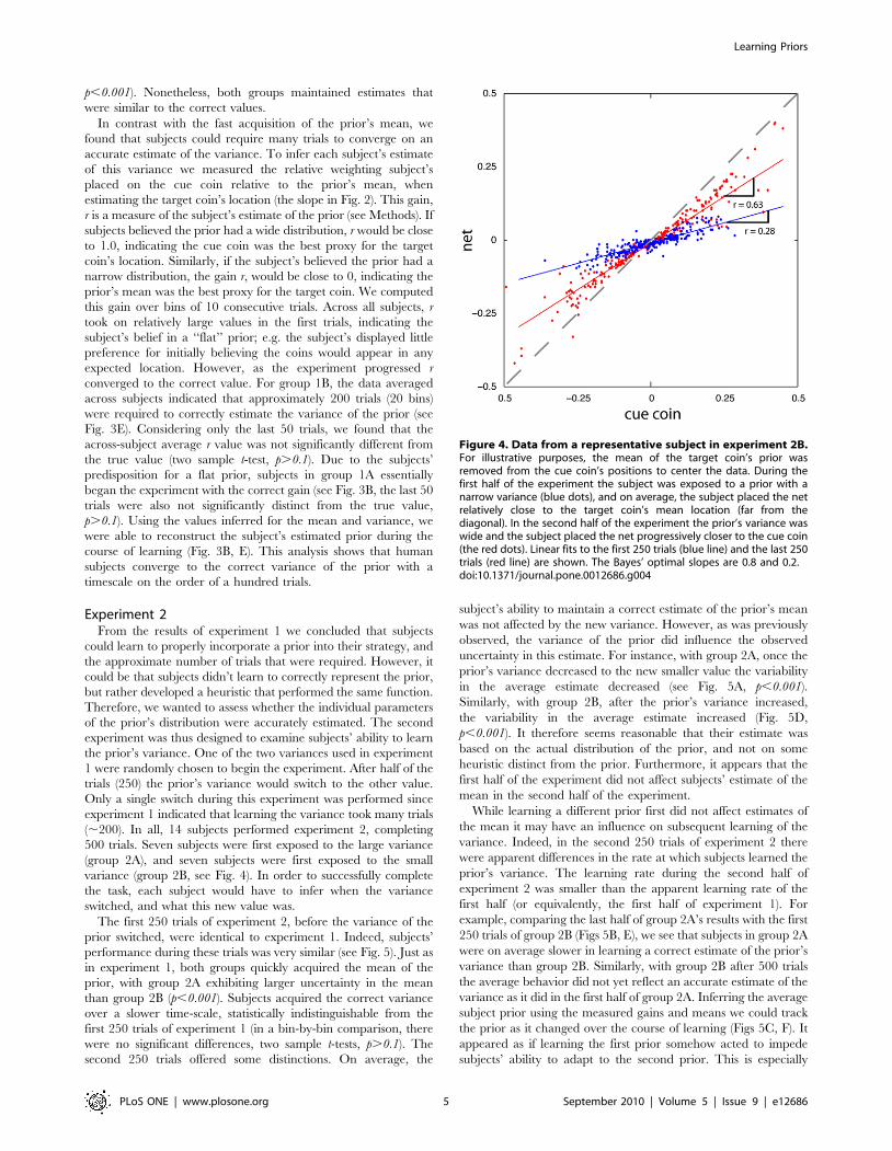
The first 250 trials of experiment 2, before the variance of the

prior switched, were identical to experiment 1. Indeed, subjects’

performance during these trials was very similar (see Fig. 5). Just as

in experiment 1, both groups quickly acquired the mean of the

prior, with group 2A exhibiting larger uncertainty in the mean

than group 2B (p,0.001). Subjects acquired the correct variance

over a slower time-scale, statistically indistinguishable from the

first 250 trials of experiment 1 (in a bin-by-bin comparison, there

were no significant differences, two sample t-tests, p.0.1). The

second 250 trials offered some distinctions. On average, the

subject’s ability to maintain a correct estimate of the prior’s mean

was not affected by the new variance. However, as was previously

observed, the variance of the prior did influence the observed

uncertainty in this estimate. For instance, with group 2A, once the

prior’s variance decreased to the new smaller value the variability

in the average estimate decreased (see Fig. 5A, p,0.001).

Similarly, with group 2B, after the prior’s variance increased,

the variability in the average estimate increased (Fig. 5D,

p,0.001). It therefore seems reasonable that their estimate was

based on the actual distribution of the prior, and not on some

heuristic distinct from the prior. Furthermore, it appears that the

first half of the experiment did not affect subjects’ estimate of the

mean in the second half of the experiment.

While learning a different prior first did not affect estimates of

the mean it may have an influence on subsequent learning of the

variance. Indeed, in the second 250 trials of experiment 2 there

were apparent differences in the rate at which subjects learned the

prior’s variance. The learning rate during the second half of

experiment 2 was smaller than the apparent learning rate of the

first half (or equivalently, the first half of experiment 1). For

example, comparing the last half of group 2A’s results with the first

250 trials of group 2B (Figs 5B, E), we see that subjects in group 2A

were on average slower in learning a correct estimate of the prior’s

variance than group 2B. Similarly, with group 2B after 500 trials

the average behavior did not yet reflect an accurate estimate of the

variance as it did in the first half of group 2A. Inferring the average

subject prior using the measured gains and means we could track

the prior as it changed over the course of learning (Figs 5C, F). It

appeared as if learning the first prior somehow acted to impede

subjects’ ability to adapt to the second prior. This is especially

Figure 4. Data from a representative subject in experiment 2B.For illustrative purposes, the mean of the target coin’s prior wasremoved from the cue coin’s positions to center the data. During thefirst half of the experiment the subject was exposed to a prior with anarrow variance (blue dots), and on average, the subject placed the netrelatively close to the target coin’s mean location (far from thediagonal). In the second half of the experiment the prior’s variance waswide and the subject placed the net progressively closer to the cue coin(the red dots). Linear fits to the first 250 trials (blue line) and the last 250trials (red line) are shown. The Bayes’ optimal slopes are 0.8 and 0.2.doi:10.1371/journal.pone.0012686.g004

Learning Priors

PLoS ONE | www.plosone.org 5 September 2010 | Volume 5 | Issue 9 | e12686

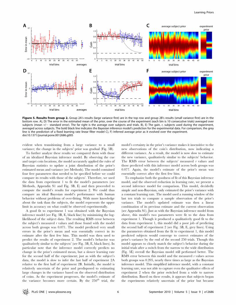
evident when transitioning from a large variance to a small

variance; the change in the subjects’ prior was gradual (Fig. 5B).

To further analyze these results we compared them with those

of an idealized Bayesian inference model. By observing the cue

and target coin locations, the model accurately applied the rules of

Bayesian statistics to update a joint distribution of the prior’s

estimated mean and variance (see Methods). The model contained

four free parameters that needed to be specified before we could

compare its results with those of the subjects’. Therefore, we used

the data from experiment 1 to fit the model’s parameters (see

Methods, Appendix S1 and Fig. 3B, E) and then proceeded to

compute the model’s results for experiment 2. We could thus

compare an ideal Bayesian model’s performance with human

behavior without problems of over-fitting. With more knowledge

about the task than the subjects, the model represents the upper

limit in accuracy on what could be observed experimentally.

A good fit to experiment 1 was obtained with the Bayesian

inference model (see Fig. 3B, E, black line) by minimizing the log-

likelihood of the subject data. The resulting RMS error between

the subject’s measured r values and those found with the model

across both groups was 0.071. The model predicted very small

errors in the prior’s mean and was essentially correct in its

estimate after the first few bins. This model was then used to

predict the results of experiment 2. The model’s behavior was

qualitatively similar to the subjects’ (see Fig. 5B, E, black lines). In

particular note that the inference model correctly predicts no

change in the prior’s estimated mean, but a slower learning rate

for the second half of the experiment; just as with the subject’s

data, the model is slow to infer the last half of experiment 2A

relative to the first half of experiment 2B. Initially, the model is

relatively uncertain of the prior and predisposed to estimating

large changes in the variance based on the observed distribution

of coins. As the experiment progresses, the model’s estimate of

the variance becomes more certain. By the 250th trial, the

model’s certainty in the prior’s variance makes it insensitive to the

new observations of the coin’s distribution, now indicating a

different variance. As a result, the model is now slow to estimate

the new variance, qualitatively similar to the subjects’ behavior.

The RMS error between the subjects’ measured r values and

those predicted with this inference model across both groups was

0.077. Again, the model’s estimate of the prior’s mean was

essentially correct after the first few bins.

To emphasize both the goodness of fit of this Bayesian inference

model, and the observed reduction in learning rate, we present a

second inference model for comparison. This model, decidedly

simple and non-Bayesian, only estimated the prior’s variance with

a constant learning rate. The model used a running window of the

last ten trials to compute a sample observation of the prior’s

variance. The model’s updated estimate was then a linear

combination of its previous estimate and the current observation

(see Appendix S1). Just as with the Bayesian inference model from

above, this model’s two parameters were fit to the data from

experiment 1. Though it produced a qualitatively good fit to the

data from experiment 1, this model did a poor job of predicting

the second half of experiment 2 (see Fig. 5B, E, grey lines). Using

the parameters obtained from the fit to experiment 1, this model

predicted subjects would converge to correct estimates of the

prior’s variance by the end of the second 250 trials. Though this

model appears to closely match the subject’s behavior during the

initial trials after a switch from the narrow to the wide distribution

(Fig. 5E) overall the Bayesian model still performed better. The

RMS error between this model and the measured r values across

both groups was 0.205, nearly three times as large as the Bayesian

inference model. This simplified inference model, with a constant

learning rate, was not able to capture even the qualitative effects of

experiment 2 when the prior switched from a wide to narrow

distribution. Based on these results, it appears that subjects began

the experiments relatively uncertain of the prior but became

Figure 5. Results from group 2. Group 2A’s results (large variance first) are in the top row and group 2B’s results (small variance first) are in thebottom row. A), D) The error in the estimated mean of the prior, over the course of the experiment (each bin is 10 consecutive trials) averaged oversubjects (mean +/2 standard error). The far right is the average over subjects and trials. B), E) The gain, r, subjects used during the experiment,averaged across subjects. The bold black line indicates the Bayesian inference model’s prediction for the experimental data. For comparison, the greyline is the prediction of a fixed learning rate linear filter model C), F) Inferred average prior as it evolved over the experiment.doi:10.1371/journal.pone.0012686.g005

Learning Priors

PLoS ONE | www.plosone.org 6 September 2010 | Volume 5 | Issue 9 | e12686

increasingly certain as the experiment progressed. This accounts

for the apparent slower learning rate later in the experiments.

Experiment 3The third experiment was designed to examine a subject’s

ability to learn the prior’s mean independent of the variance. We

held the variance of the prior constant but changed its mean. At

the start of the experiment, the mean of the prior was randomly

chosen between one of two locations. Each subject was exposed to

a minimum of 10 consecutive trials with the same prior after which

there was a small probability the mean would switch to the other

value on any trial. Over the course of the experiment each subject

would be exposed to approximately 50 of these changes in the

prior’s mean. Ten subjects performed the experiment (600 trials)

after being given the same instructions as in the previous

experiments above (see Methods). As in the previous experiments,

subjects would have to infer when the mean switched, and what

the new value of this mean was in order to successfully complete

the task.

Just as in the previous two experiments, subjects quickly

acquired an accurate estimate of the mean even though it

switched frequently. In contrast to the previous analysis, we

wanted to examine the temporal aspects of this estimate on the

relatively fast time scale of single trials rather than bins of 10 trials.

For each subject we resorted the data, locked on the first trial after

a switch in the prior’s mean. This allowed us to observe the

subjects estimate of the mean on a trial-by-trial basis. We then

averaged theses estimates of the prior’s mean across all ten subjects

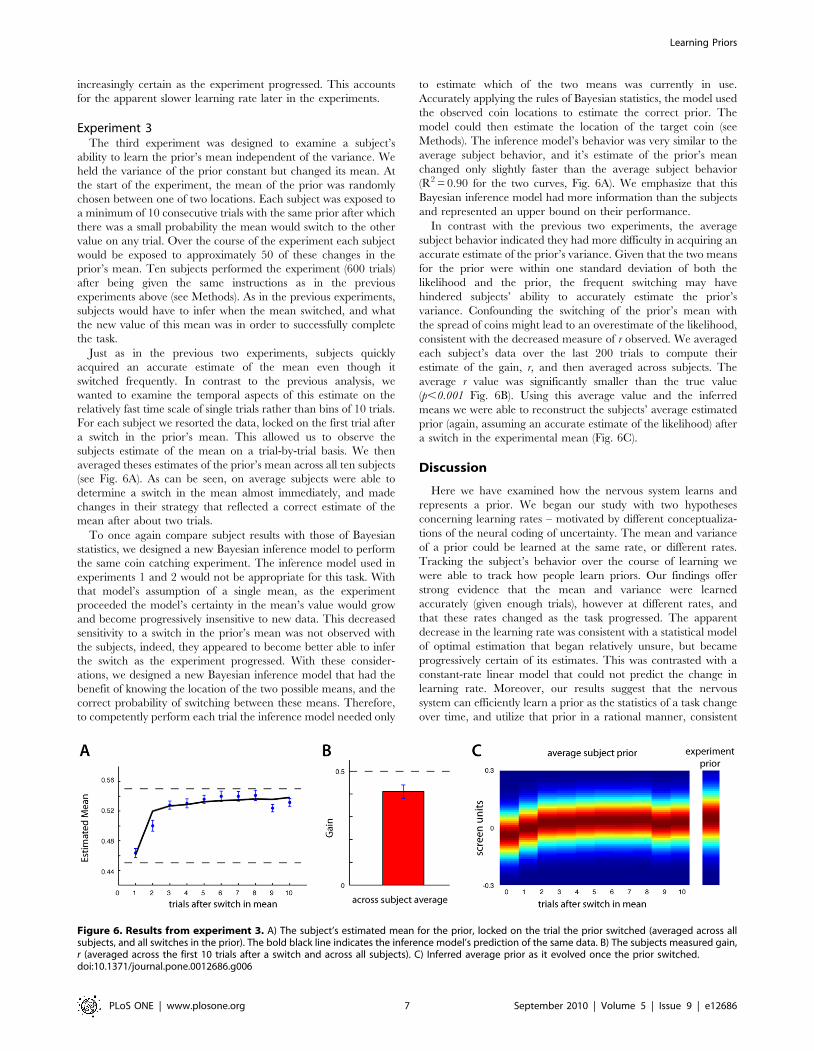
(see Fig. 6A). As can be seen, on average subjects were able to

determine a switch in the mean almost immediately, and made

changes in their strategy that reflected a correct estimate of the

mean after about two trials.

To once again compare subject results with those of Bayesian

statistics, we designed a new Bayesian inference model to perform

the same coin catching experiment. The inference model used in

experiments 1 and 2 would not be appropriate for this task. With

that model’s assumption of a single mean, as the experiment

proceeded the model’s certainty in the mean’s value would grow

and become progressively insensitive to new data. This decreased

sensitivity to a switch in the prior’s mean was not observed with

the subjects, indeed, they appeared to become better able to infer

the switch as the experiment progressed. With these consider-

ations, we designed a new Bayesian inference model that had the

benefit of knowing the location of the two possible means, and the

correct probability of switching between these means. Therefore,

to competently perform each trial the inference model needed only

to estimate which of the two means was currently in use.

Accurately applying the rules of Bayesian statistics, the model used

the observed coin locations to estimate the correct prior. The

model could then estimate the location of the target coin (see

Methods). The inference model’s behavior was very similar to the

average subject behavior, and it’s estimate of the prior’s mean

changed only slightly faster than the average subject behavior

(R2 = 0.90 for the two curves, Fig. 6A). We emphasize that this

Bayesian inference model had more information than the subjects

and represented an upper bound on their performance.

In contrast with the previous two experiments, the average

subject behavior indicated they had more difficulty in acquiring an

accurate estimate of the prior’s variance. Given that the two means

for the prior were within one standard deviation of both the

likelihood and the prior, the frequent switching may have

hindered subjects’ ability to accurately estimate the prior’s

variance. Confounding the switching of the prior’s mean with

the spread of coins might lead to an overestimate of the likelihood,

consistent with the decreased measure of r observed. We averaged

each subject’s data over the last 200 trials to compute their

estimate of the gain, r, and then averaged across subjects. The

average r value was significantly smaller than the true value

(p,0.001 Fig. 6B). Using this average value and the inferred

means we were able to reconstruct the subjects’ average estimated

prior (again, assuming an accurate estimate of the likelihood) after

a switch in the experimental mean (Fig. 6C).

Discussion

Here we have examined how the nervous system learns and

represents a prior. We began our study with two hypotheses

concerning learning rates – motivated by different conceptualiza-

tions of the neural coding of uncertainty. The mean and variance

of a prior could be learned at the same rate, or different rates.

Tracking the subject’s behavior over the course of learning we

were able to track how people learn priors. Our findings offer

strong evidence that the mean and variance were learned

accurately (given enough trials), however at different rates, and

that these rates changed as the task progressed. The apparent

decrease in the learning rate was consistent with a statistical model

of optimal estimation that began relatively unsure, but became

progressively certain of its estimates. This was contrasted with a

constant-rate linear model that could not predict the change in

learning rate. Moreover, our results suggest that the nervous

system can efficiently learn a prior as the statistics of a task change

over time, and utilize that prior in a rational manner, consistent

Figure 6. Results from experiment 3. A) The subject’s estimated mean for the prior, locked on the trial the prior switched (averaged across allsubjects, and all switches in the prior). The bold black line indicates the inference model’s prediction of the same data. B) The subjects measured gain,r (averaged across the first 10 trials after a switch and across all subjects). C) Inferred average prior as it evolved once the prior switched.doi:10.1371/journal.pone.0012686.g006

Learning Priors

PLoS ONE | www.plosone.org 7 September 2010 | Volume 5 | Issue 9 | e12686

with the predictions of a Bayesian inference model. While many

studies have assumed that subjects learn priors, we have measured

in detail how human subjects do so. Our results offer evidence that

people can form an accurate prior, estimating its mean and

variance.

This study was a first attempt to examine the temporal

characteristics of how subjects acquire an estimate of the prior.

To keep the scope of the paper manageable, we used a normal

distribution for the experimental prior and the likelihood. Under

these conditions a Bayes’ optimal inference of the target coin’s

location is a linear function of the cue coin’s location. Indeed, only

two numbers were required to infer the target coin’s location: an

offset term and a slope (the gain r). The simple form of this Bayes’

optimal solution confounds our ability to infer whether or not the

subjects were precisely estimating the experimental prior. For

instance, it could be the case that subjects do not actually learn

accurate priors, but instead attempt to estimate all distributions as

Gaussian, merely estimating the mean and the variance. Or in an

even more uncomplicated fashion, it could be the case that subjects

bypass the process of representing a prior and a likelihood

altogether and merely estimate the resulting two parameters that

were necessary for the optimal inference. However, we have several

reasons to believe this is not the case, and subjects actually attempt

to accurately represent the necessary statistics. Based on prior

research, it is known that subjects react to changes in the statistics of

both the prior and the likelihood. In one study in particular, when

subjects were confronted with non-Gaussian distributions their

behavior became predictably nonlinear [5]. This argues against a

simple linear fit to the cue and target coins. Furthermore, when

subjects in that study were presented with new likelihoods, they

generalized in a Bayes’ appropriate manner; implying subjects had

learned the prior and not simply r. Finally, from a computational

standpoint, the value r (which is defined with ratio of two random

Gaussian variables) has a non-Gaussian distribution with a large

second moment. Inferring this variable directly and accurately is

therefore an unwarranted complication. Future studies could

investigate the degree to which subjects accurately represent a

prior and likelihood, or use approximating heuristics.

In all 3 experiments, subjects see both the cue and target coins

simultaneously, on each trial. Therefore subjects can directly

observe the spread of the likelihood, and receive many such

observations. Samples from the prior, on the other hand, are not

directly observed, but must be gathered from trial to trial. Based

on these considerations, and the findings of similar work discussed

above, we assumed subjects quickly estimated the likelihood of the

variance, and that the dynamics of the learning process were

dominated by the estimation of the prior. Assuming these

considerations are valid, our study addresses the learning of

priors. However, future studies could specifically examine just how

quickly subjects accurately acquire an estimate of the likelihood.

Overall, subjects were able to quickly learn the mean of a prior.

Relative to a Bayesian inference model, the subjects performed

especially well when the mean of the prior switched repeatedly

(experiment 3). The inference model, having perfect knowledge of

the two possible means, merely estimated which one was currently

most likely. Based on the subjects’ performance, it appears they

may have done the same thing; that is, rather than continuously

inferring the mean based on the evidence, subjects remembered

two possible means and estimated which one was being employed.

It is plausible that after the subjects had been exposed to the two

means repeatedly they inferred the causal structure of the task

[4,7,16,17]. Human behavior appears to approximate that of an

optimal observer and the nervous system thus appears to use

powerful learning algorithms.

There may be both statistical and neurobiological reasons for

our finding that subjects took longer to learn the variance than the

mean of the prior. From a statistical point of view, an accurate

estimate of the variance requires more samples than that of the

mean. Therefore, the relatively slow convergence to a correct

variance for the prior is understandable. It could also be that

subjects have real world experience that suggests phenomena

change over relatively slow time scales. In addition, subjects

displayed an inclination for assuming a flat prior at the outset of

the experiment. Again, this could be based on real world

experiences for preferring broad distributions. From a computa-

tional standpoint, it could be seen as a sensible strategy as well,

neglecting a prior (or equivalently, assuming a flat prior) results in

a maximum likelihood strategy (rather than a full Bayesian

estimate). From a neurobiological point of view we may also

expect different learning rates. Various lines of research investi-

gating the rapid learning of a perturbation (mean) have implicated

the cerebellum [18,19,20]. Other studies have found that

uncertainty (variance) may be represented in the Basal ganglia

and area LIP (e.g., [21,22]). These areas may well exhibit slower

learning than the cerebellum. The combination of these different

neural structures may give rise to rapid learning of means and

slower learning of variance.

We also see both statistical and neurobiological reasons for the

finding that subjects were slower to adapt as the experiment

progressed. The inference model, accurately applying the rules of

Bayesian statistics, grew more certain of the prior as the

experiment progressed. As a result, the model was slower to react

to a change in the prior during the second half of the experiment.

The subjects appear to be utilizing a similar strategy, perhaps

growing more confident in their beliefs and less sensitive to their

observations. This finding, of a change in the learning rate as the

uncertainty in parameters changes is also consistent with a

growing body of experimental evidence. Recent findings suggest

specific cortical structures may represent a subject’s level of

uncertainty in task parameters [13,14,22,23]. Further evidence

proposes that neuromodulators may also encode uncertainty

[15,21]. These representations of uncertainty may allow the

nervous system to learn relatively rapidly at the outset of the

experiment, when subjects are generally uncertain of the task [24].

As the experiment progresses and subjects grow more confident in

their beliefs the nervous system may learn more slowly.

In addition to the time-varying adaptation rate, it appeared as if

subjects adapted asymmetrically to increases and decreases in a

prior’s variance, ostensibly reacting more quickly when the

variance abruptly increased (Fig. 5E). Our Bayesian inference

model employed a relatively simple generative model sufficient to

explain the time-varying character of adaptation we focused on.

Interestingly, this same asymmetric phenomena has been

described in computational models of optimal Bayesian estimation

of variance [25]. What’s more, these same asymmetries have been

observed in neural data when adapting to similar changes in the

variance of a stimulus [26]. Together with our data, these

theoretical and phenomenological findings offer evidence that the

nervous system employs near optimal estimation of the statistics of

stimuli.

Both the average subject performance and the Bayesian

modeling indicated subjects quickly acquired the mean of the

prior. However, in contrast with the Bayesian model, subjects

continued to display relatively large amounts of variance in this

estimate throughout the course of the experiments. If subjects

believed the statistics of the experiment to be stationary, their

variance ought to have decreased as the experiment proceeded.

This was not evident. It could be that although subjects believe the

Learning Priors

PLoS ONE | www.plosone.org 8 September 2010 | Volume 5 | Issue 9 | e12686

environment is stationary they exhibit ‘‘non-Bayesian’’ behavior

periodically. A well-known instance of this is the so-called

matching behavior [27]. In our experiment, subjects could be

exhibiting a similar phenomenon, making choices that are

inconsistent with a maximum a posteriori estimate. Further, it could

be that subjects don’t strictly believe in stationary distributions,

and instead entertain the possibility that changes may occur. This

would imply their uncertainty (and resulting variance) should

remain non-zero even at steady-state. This too would be consistent

with their behavior.

The coin catching experiment is a task requiring both an

inference (where is the target coin?), and a subsequent decision

based on this inference (where should the net be placed?). That is,

strictly speaking, subjects might be weighing their decision of

where to place the net against concerns other than where they

believe the target most likely to lie; e.g. how much effort is takes to

move the net where they believe the target will be. Theoretically,

in describing subjects’ behavior we must invoke a loss or value

function. However, our task was designed such that there was

minimal motor effort (turning the paddle wheel). As a result, our

task was effectively an estimation problem and using Bayesian

algorithms we modeled it as such. Moreover, subjects’ behavior

might depend on other factors such as visual acuity. By displaying

relatively large coins with striking colors against a relatively neutral

back-drop, and having subjects seated closely in front of the

computer monitor, the experiment attempted to minimize this

internal measurement noise relative to the experimentally

controlled cue coin variance. In these ways, the task was designed

to be a probe for subjects’ priors and to minimize the influence of

other factors.

Tracking changing priors may open the possibility for new

analyses in neural representations in sensorimotor tasks. Properties

such as external stimuli or motor behaviors may be far ‘‘up’’, or

‘‘downstream’’ from their neural representations, depending on

where in the brain data is recorded from. However, pairing

electrophysiological studies with the analysis performed here

provides a new correlate for neural data. An evolving prior,

inferred from behavioral data, may offer a closer correlate to the

internal representations of a task and the resulting motor

outcomes. Thus this approach may offer a new way of analyzing

neural representations in a wide range of perceptual, motor, and

perhaps cognitive tasks.

Priors characterize the beliefs human subjects maintain and are

integral to how we decide upon actions and form decisions. Some

recent models of neurological diseases such as schizophrenia are

now applying the quantitative strategies of Bayesian statistics

[28,29]. Using the strategies developed in this study may thus offer

novel ways of analyzing the mechanisms that give rise to

neurological deficits.

Supporting Information

Appendix S1

Found at: doi:10.1371/journal.pone.0012686.s001 (0.09 MB

DOC)

Author Contributions

Conceived and designed the experiments: MB MV KPK. Performed the

experiments: MB MV. Analyzed the data: MB. Wrote the paper: MB MV

KPK.

References

1. Weiss Y, Simoncelli EP, Adelson EH (2002) Motion illusions as optimal percepts.

Nat Neurosci 5: 598–604.

2. Stocker AA, Simoncelli EP (2006) Noise characteristics and prior expectations in

human visual speed perception. Nat Neurosci 9: 578–585.

3. Jacobs RA (1999) Optimal integration of texture and motion cues to depth.

Vision Res 39: 3621–3629.

4. Kording KP, Beierholm U, Ma WJ, Quartz S, Tenenbaum JB, et al. (2007)

Causal inference in multisensory perception. PLoS ONE 2: e943.

5. Kording KP, Wolpert DM (2004) Bayesian integration in sensorimotor learning.

Nature 427: 244–247.

6. Miyazaki M, Nozaki D, Nakajima Y (2005) Testing Bayesian models of human

coincidence timing. J Neurophysiol 94: 395–399.

7. Hudson TE, Maloney LT, Landy MS (2007) Movement planning with

probabilistic target information. J Neurophysiol 98: 3034–3046.

8. Berniker M, Kording K (2008) Estimating the sources of motor errors for

adaptation and generalization. Nat Neurosci 11: 1454–1461.

9. Adams WJ, Graf EW, Ernst MO (2004) Experience can change the ‘light-from-

above’ prior. Nat Neurosci 7: 1057–1058.

10. Tassinari H, Hudson TE, Landy MS (2006) Combining priors and noisy visual

cues in a rapid pointing task. J Neurosci 26: 10154–10163.

11. Thoroughman KA, Shadmehr R (2000) Learning of action through adaptive

combination of motor primitives. Nature 407: 742–747.

12. Kawato M, Furukawa K, Suzuki R (1987) A hierarchical neural-network model

for control and learning of voluntary movement. Biol Cybern 57: 169–185.

13. Behrens TE, Woolrich MW, Walton ME, Rushworth MF (2007) Learning the

value of information in an uncertain world. Nat Neurosci 10: 1214–1221.

14. Kiani R, Shadlen MN (2009) Representation of confidence associated with a

decision by neurons in the parietal cortex. Science 324: 759–764.

15. Yu AJ, Dayan P (2005) Uncertainty, neuromodulation, and attention. Neuron

46: 681–692.

16. Wei K, Kording K (2009) Relevance of error: what drives motor adaptation?J Neurophysiol 101: 655–664.

17. Tenenbaum JB, Griffiths TL, Kemp C (2006) Theory-based Bayesian models ofinductive learning and reasoning. Trends Cogn Sci 10: 309–318.

18. Chen H, Hua SE, Smith MA, Lenz FA, Shadmehr R (2006) Effects of humancerebellar thalamus disruption on adaptive control of reaching. Cereb Cortex

16: 1462–1473.

19. Nezafat R, Shadmehr R, Holcomb HH (2001) Long-term adaptation todynamics of reaching movements: a PET study. Exp Brain Res 140: 66–76.

20. Lewis RF, Tamargo RJ (2001) Cerebellar lesions impair context-dependentadaptation of reaching movements in primates. Exp Brain Res 138: 263–267.

21. Schultz W, Preuschoff K, Camerer C, Hsu M, Fiorillo CD, et al. (2008) Explicit

neural signals reflecting reward uncertainty. Philos Trans R Soc Lond B Biol Sci363: 3801–3811.

22. Churchland AK, Kiani R, Shadlen MN (2008) Decision-making with multiplealternatives. Nat Neurosci 11: 693–702.

23. Rushworth MF, Behrens TE (2008) Choice, uncertainty and value in prefrontaland cingulate cortex. Nat Neurosci 11: 389–397.

24. Burge J, Ernst MO, Banks MS (2008) The statistical determinants of adaptation

rate in human reaching. J Vis 8: 20 21–19.25. DeWeese M, Zador A (1998) Asymmetric Dynamics in Optimal Variance

Adaptation. Neural Computation 10: 1179–1202.26. Fairhall AL, Lewen GD, Bialek W, de Ruyter Van Steveninck RR (2001)

Efficiency and ambiguity in an adaptive neural code. Nature 412: 787–792.

27. Sugrue LP, Corrado GS, Newsome WT (2004) Matching behavior and therepresentation of value in the parietal cortex. Science 304: 1782–1787.

28. Fletcher PC, Frith CD (2009) Perceiving is believing: a Bayesian approach toexplaining the positive symptoms of schizophrenia. Nat Rev Neurosci 10: 48–58.

29. Dima D, Roiser JP, Dietrich DE, Bonnemann C, Lanfermann H, et al. (2009)Understanding why patients with schizophrenia do not perceive the hollow-mask

illusion using dynamic causal modelling. Neuroimage.

Learning Priors

PLoS ONE | www.plosone.org 9 September 2010 | Volume 5 | Issue 9 | e12686