Simulation and implementation of grid-connected inverters

International Journal of Computer Applications (0975 – 8887)

Volume 60– No.4, December 2012

41

Simulation and Implementation of

Grid-connected Inverters

Ahmed Abdalrahman Engineer

Dept. of Electronics & Communications Engineering,

Thebes higher institute of Engineering, Cairo, Egypt.

Abdalhalim Zekry Professor


Faculty of Engineering, Ain-shams University,

Cairo, Egypt.

Ahmed Alshazly Lecturer


Thebes higher institute of Engineering, Cairo, Egypt.

ABSTRACT

Solar, wind and hydro are renewable energy sources that are

seen as reliable alternatives to conventional energy sources

such as oil or natural gas. However, the efficiency and the

performance of renewable energy systems are still under

development. Consequently, the control structures of the grid-

connected inverter as an important section for energy

conversion and transmission should be improved to meet the

requirements for grid interconnection. In this paper, a

comprehensive simulation and implementation of a three-

phase grid-connected inverter is presented. The control

structure of the grid-side inverter is firstly discussed.

Secondly, the space vector modulation SVM is presented.

Thirdly, the synchronization for grid-connected inverters is

discussed. Finally, the simulation of the grid-connected

inverter system using PSIM simulation package and the

system implementation are presented to illustrate concepts

and compare their results.

General Terms

Control systems, Embedded systems, Power electronics,

Renewable energy.

Keywords

Grid-connected inverter, synchronous PI controller, SVM,

PLL, PSIM.

1. INTRODUCTION

Fossil fuels and hydropower along with non-commercial fuels

such as firewood are considered the main energy resources in

Egypt. However, Because of the growing demand in fossil

fuel resources and the resulting environmental effects, Egypt’s

energy strategy aims to increase the reliance on renewable

energy sources, particularly wind and concentrated solar

power. Consequently, the national energy plan aims to

achieve 20% of total generated electricity from renewable

energy sources by the year 2020 including 12% from wind

energy. This expected to be achieved through establishing

grid-connected wind farms and solar photovoltaic (PV)

systems [1].

Most of renewable energy technology produces a DC power

output. An inverter is needed to convert the DC electric

energy from the renewable energy source into AC electric

energy. The inverters are either stand-alone [2],[3], or grid-

connected [4], In case of grid-connected inverter, the inverter

output voltage and frequency should be the same as that of the

grid voltage and frequency. Consequently, the control of the

inverter should be improved to meet the requirements for grid

interconnection.

In [5] it is stated that the control tasks of the grid-connected

inverter can be divided into two parts: Input-side controller

and Grid-side controller. The control objective on the Input-

side controller is to capture maximum power from the input

source. However, the control objectives on the Grid-side

controller are to control the power delivered to the grid,

ensure high quality of the injected power and Grid

synchronization.

A number of papers, such as [6], [7], [8], deal with control of

the grid side inverter, which use current control loop to

regulate the grid current. In other works, the control of the

grid-connected inverter is based on two cascaded loops: an

internal current loop, which regulates the grid current, and an

external voltage loop, which is designed for balancing the

power flow in the system [5]. Moreover, control strategies

employing an outer power controller and an inner current

control loop are also reported [9].

In this paper, a comprehensive study of a three-phase grid-

connected inverter with grid side controller is presented. To

carry this out, the whole inverter system is modeled and

simulated using PSIM simulation package, while taking into

consideration the non-ideal behavior of the constituting

elements of the inverter. In addition, the practical

implementation is provided to verify the simulation results.

The paper is organized as follows: the theory of the three-

phase grid-connected inverter is discussed in Section 2. This

consists of the control theory of the grid-side inverter. In

addition, the space vector modulation SVM is presented.

Moreover, it explains the synchronization method for grid-

connected power inverters. Inverter simulation and

implementation are provided in Sections 3 and 4 respectively.

Finally, Summary and conclusions are provided in Section 5.

2. THE THEORY OF THE THREE-

PHASE GRID-CONNECTED INVERTER

In order to control three-phase voltage-source inverters (VSI),

there are two control strategies: current control and voltage

control. The voltage-controlled VSI use the phase angle

between the inverter output voltage and the grid voltage to

control the power flow. In the current controlled VSI, the

active and reactive components of the current injected into the

grid are controlled using pulse width modulation (PWM)

techniques. A current controller is less sensitive to voltage

phase shifts and to distortion in the grid voltage. Moreover, it

is faster in response. On the other hand, the voltage control is



42

sensitive to small phase errors and large harmonic currents

may occur if the grid voltage is distorted. Consequently, the

current control is recommended in the control of grid-

connected inverter [10].

The current controller of three-phase VSI plays an essential

part in controlling grid-connected inverters. Consequently, the

quality of the applied current controller largely influences the

performance of the inverter system. Many control

mechanisms have been proposed to regulate the inverter

output current that is injected into the utility grid. Among

these control mechanisms, three major types of current

controller have evolved: hysteresis controller, predictive

controller and linear proportional-integral (PI) controller.

Predictive controller has a very good steady-state performance

and provides a good dynamic performance. However, its

performance is sensitive to system parameters. The hysteresis

controller has a fast transient response, non-complex

implementation and an inherent current protection. However,

the hysteresis controller has some drawbacks such as variable

switching frequency and high current ripples. These cause a

poor current quality and introduce difficulties in the output

filter design [7], [11].

The PI controller is the most common control algorithm used

for current error compensation. A PI controller calculates an

error value as the difference between a measured inverter

output current and a desired injected current to the grid, then

the controller attempts to minimize the error between them.

The PI controller calculation algorithm involves two separate

constant parameters, the proportional constant Kp and the

integral constant Ki. The proportional term of the controller is

formed by multiplying the error signal by a Kp gain. This

tends to reduce the overall error with time. However, the

effect of the proportional term will not reduce the error to

zero, and there is some steady stat error. The Integral term of

the controller is used to fix small steady state errors. The

Integral term integrates the error then multiplies it by a Ki

constant and becomes the integral output term of the PI

controller. This removes the steady state error and accelerates

the movement of the process into the reference point.

The PI current control offers an excellent steady-state

response, low current ripple, constant switching frequency, in

addition to well-defined harmonic content. Moreover, the

controller is insensitive to system parameters since the

algorithm does not need system models [7]. PI controllers can

be applied either in the stationary (αβ) or in synchronous (dq)

reference frame. When the synchronous PI controller is used,

the control variables become DC and the PI compensators are

able to reduce the stationary error of the fundamental

component to zero. This is not the case with PI controllers

working in the stationary system, where there is an inherent

tracking error of phase and amplitude. Therefore, current

control in a synchronous (rotating) reference frame, using PI

controllers is the typical solution in the three‐phase grid-

connected inverters [11].

According to the mathematical model of the grid-connected

inverter [8], the output voltages of the inverter in the

synchronous (dq) frame are given by

where ed and eq are the components of the park

transformation of the grid voltage. ud and uq are the

components of the park transformation of the inverter output.

ω is the angular frequency of the grid. L is the inductance

between the grid-connected inverter and the grid. R is the

resistance between the grid-connected inverter and the grid.

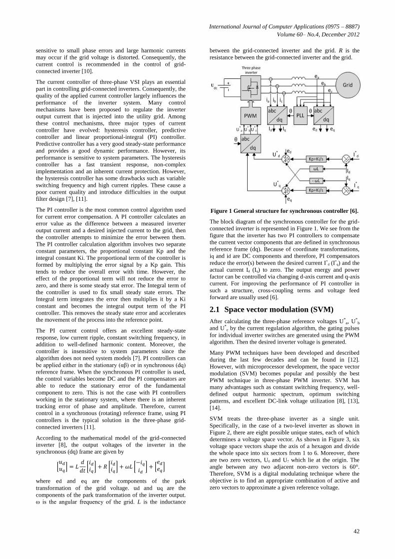
Figure 1 General structure for synchronous controller [6].

The block diagram of the synchronous controller for the grid-

connected inverter is represented in Figure 1. We see from the

figure that the inverter has two PI controllers to compensate

the current vector components that are defined in synchronous

reference frame (dq). Because of coordinate transformations,

iq and id are DC components and therefore, PI compensators

reduce the error(s) between the desired current I*d (I

*q) and the

actual current Id (Iq) to zero. The output energy and power

factor can be controlled via changing d-axis current and q-axis

current. For improving the performance of PI controller in

such a structure, cross-coupling terms and voltage feed

forward are usually used [6].

2.1 Space vector modulation (SVM)

After calculating the three-phase reference voltages U*a, U*

b

and U*c by the current regulation algorithm, the gating pulses

for individual inverter switches are generated using the PWM

algorithm. Then the desired inverter voltage is generated.

Many PWM techniques have been developed and described

during the last few decades and can be found in [12].

However, with microprocessor development, the space vector

modulation (SVM) becomes popular and possibly the best

PWM technique in three-phase PWM inverter. SVM has

many advantages such as constant switching frequency, well-

defined output harmonic spectrum, optimum switching

patterns, and excellent DC-link voltage utilization [8], [13],

[14].

SVM treats the three-phase inverter as a single unit.

Specifically, in the case of a two-level inverter as shown in

Figure 2, there are eight possible unique states, each of which

determines a voltage space vector. As shown in Figure 3, six

voltage space vectors shape the axis of a hexagon and divide

the whole space into six sectors from 1 to 6. Moreover, there

are two zero vectors, U0 and U7 which lie at the origin. The

angle between any two adjacent non-zero vectors is 60°.

Therefore, SVM is a digital modulating technique where the

objective is to find an appropriate combination of active and

zero vectors to approximate a given reference voltage.



43

Figure 2 Two-level three-phase inverter configuration

Figure 3 Six active vectors and two null vectors in SVM.

In SVM, the three-phase reference voltages U*a, U

*b, and U*

c

are mapped to the complex two-phase orthogonal (αβ) plane.

This is known as the Clark’s transformation.

The construction of any space vector Uref which lies in the

hexagon can be done by time averaging the adjacent two

active space vectors and any zero vectors, as follows

where Un and Un+1 are the non-zero adjacent active vectors. U0

and U7 are the zero vectors. T1, T2, T0, T7 are time-shares of

respective voltage vectors and Ts is the sampling period.

SVM can be implemented through the following steps [15]:

1. The Computation of reference voltage and angle

(θ).

θ

2. Identification of sector number that is done by

taking the angle computed from the last step, and

then comparing it with angles range of each sector.

3. Calculate the modulation index ( ) and the time

duration T1, T2, T0, T7.

θ

θ

4. After T1, T2, T7, and T0 are calculated; the SVM

pulses can be generated. The arrangement of

switching sequence must ensure minimum transition

between one vector and the next. This method

reduces the switching frequency and has fewer

harmonics. For sector 1, one can use 01277210 for

symmetry reasons as shown in Figure 4.

Figure 4 SVM switching patterns for sector 1.

2.2 Grid synchronization

The inverter output current that is injected into the utility

network must be synchronized with the grid voltage. The

objective the synchronization algorithm is to extract the phase

angle of the grid voltage. The feedback variables can be

converted into a suitable reference frame using the extracted

grid angle. Hence, the detection of the grid angle plays an

essential role in the control of the grid-connected inverter [5],

[6]. The synchronization algorithms should respond quickly to

changes in the utility grid. Moreover, they should have the

ability to reject noise and the higher order harmonics. Many

synchronization algorithms have been proposed to extract the

phase angle of the grid voltage such as zero crossing

detection, and phase-locked loop (PLL).

The simplest synchronization algorithm is the zero crossing

detection. However, this method has many disadvantages such

as low dynamics. In addition, it is affected by noise and

higher order harmonics in the utility grid. Therefore, this

method is unsuitable for applications that require consistently

accurate phase angle detection.

Nowadays, the most common synchronization algorithm for

extracting the phase angle of the grid voltages is the PLL. The

PLL can successfully detect the phase angle of the grid

voltage even in the presence of noise or higher order

harmonics in the grid.



44

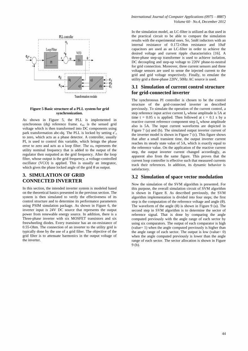
Figure 5 Basic structure of a PLL system for grid

synchronization.

As shown in Figure 5, the PLL is implemented in

synchronous (dq) reference frame. eabc is the sensed grid

voltage which is then transformed into DC components using

park transformation abc-dq. The PLL is locked by setting e*d

to zero, which acts as a phase detector. A controller, usually

PI, is used to control this variable, which brings the phase

error to zero and acts as a loop filter. The ωff represents the

utility nominal frequency that is added to the output of the

regulator then outputted as the grid frequency. After the loop

filter, whose output is the grid frequency, a voltage-controlled

oscillator (VCO) is applied. This is usually an integrator,

which gives the phase locked angle of the grid θ as output.

3. SIMULATION OF GRID

CONNECTED INVERTER

In this section, the intended inverter system is modeled based

on the theoretical basics presented in the previous section. The

system is then simulated to verify the effectiveness of its

control structure and to determine its performance parameters

using PSIM simulation package. As shown in Figure 6, the

inverter input is 24V DC source that represents the output

power from renewable energy source. In addition, there is a

Three-phase inverter with six MOSFET transistors and six

freewheeling diodes. Every transistor has an on-resistance of

0.55-Ohm. The connection of an inverter to the utility grid is

typically done by the use of a grid filter. The objective of the

grid filter is to attenuate harmonics in the output voltage of

the inverter.

In the simulation model, an LC-filter is utilized as that used in

the practical circuit to be able to compare the simulation

results with the experimental ones. So, 5mH inductors with an

internal resistance of 0.172-Ohm resistance and 10uF

capacitors are used as an LC-filter in order to achieve the

desired voltage and current ripple characteristics [16]. A

three-phase step-up transformer is used to achieve isolation,

DC decoupling and step-up voltage to 220V phase-to-neutral

for grid connection. Moreover, three current sensors and three

voltage sensors are used to sense the injected current to the

grid and grid voltage respectively. Finally, to emulate the

utility grid a three-phase 220V, 50Hz AC source is used.

3.1 Simulation of current control structure

for grid-connected inverter

The synchronous PI controller is chosen to be the control

structure of the grid-connected inverter as described

previously. To simulate the operation of the current control, a

step reference input active current Id whose amplitude is 5A at

time t = 0.05 s is applied. Then followed at t = 0.1 s by a

reactive current reference component step Iq whose amplitude

also is 5A. The input current waveforms are depicted in

Figure 7 (a) and (b). The simulated output inverter current of

the inverter model is shown in Figure 7 (c). This figure shows

that after a small transient time, the output inverter current

reaches its steady state value of 5A, which is exactly equal to

the reference value. On the application of the reactive current

step, the output inverter current changed accordingly, as

apparent also from the same figure. This proves that the

current loop controller is effective such that measured currents

track their references. In addition, its dynamic behavior is

satisfactory.

3.2 Simulation of space vector modulation

Now the simulation of the SVM algorithm is presented. For

this purpose, the overall simulation circuit of SVM algorithm

is shown in Figure 8. As described previously, the SVM

algorithm implementation is divided into four steps; the first

step is the computation of the reference voltage and angle (θ).

The waveform of the angle (θ) is shown in Figure 9 (a). The

second step in SVM algorithm is to determine the sector of

reference signal. That is done by comparing the angle

computed previously with the angle range of each sector by

using six comparators. The output of each comparator is high

(value= 1) when the angle computed previously is higher than

the angle range of each sector. The output is low (value= 0)

when the angle computed previously is lower than the angle

range of each sector. The sector allocation is shown in Figure

9 (b).



45

Figure 6 Simulation model of the grid-connected inverter

Figure 7 (a) Id current reference and measured (b) Iq current reference and measured

(c) Simulation result of phase grid current Ia.

Figure 8 The overall simulation circuit of SVM algorithm



46

Figure 9 (a) angle calculation (b) Sector allocation

The third step in SVM algorithm is to calculate the time

durations T1, T2, T0 and T7. The time duration is calculated by

a set of equations that are a function of modulation index ( ),

angle ( ) and sampling frequency (Fs = 1/Ts) which is 3.6

KHz. The final step is to determine the pulse width for each

transistor input. The circuit contains six-monostable

multivibrators with adjustable width that allows the pulse

width to be specified externally. Each pulse with the specified

width that is calculated from the previous step is marked by

unique amplitude. Then, six two-dimensional lookup tables

are used to output the switching pulse for each transistor.

Assuming ideal transistor switches with zero on resistance,

the simulated output phase-to-neutral voltage of the grid-

connected inverter before LC-filter is shown in Figure 10.

This waveform is typical for such an inverter. To demonstrate

the effect of the filter, the output voltage waveform of the

inverter after the LC-filter is shown in Figure 11. This figure

shows that the waveform is a nearly pure sinusoidal waveform

with small ripples.

Then, in order to take into consideration the non-ideal effects

of the model component, especially the on resistances of the

transistors, the simulation is repeated with an on resistance of

0.55 Ohm. The simulated waveform of the output phase

voltage is shown in Figure 12. It is clear from the figure that

the presence of an appreciable on resistance with the power

switches causes noticeable distortion of the output voltage

waveform.

Figure 10 Inverter phase voltage at the input of the filter.

Figure 11 Inverter phase voltage considering ideal

transistors.

Figure 12 Inverter phase voltage considering non-ideal

transistors

3.3 Simulation of PLL synchronization

circuit As described previously, the PLL circuit is the best-known

synchronization algorithm. The simulation results of PLL as

shown in Figure 13 show that the PLL can successfully

extract, without errors, the phase angle of the grid voltages,

which allows for synchronization with the grid. The extracted

phase angle is used to convert the feedback variables into the

(dq) reference. Consequently, synchronization between output

of inverter phase and grid phase angle is achieved by locking

PLL for every instant of time between 0 to 2π.



47

Figure 13 (a) phase voltage of the grid. (b) PLL phase

angle.

4. EXPERIMENTAL

IMPLEMENTATION OF GRID-

CONNECTED INVERTER In this section, a complete experimental version of the

modeled inverter is presented. The major differences between

the simulation model and the experimental version are

intended to clarify. The hardware of the grid-connected

inverter platform will consist of two sections: the power

circuit and the control circuit. The power circuit consists of

the power switches and their drivers. On the other hand, the

control circuit consists of the dsPIC microcontroller with the

software of operation. The following two sections provide a

detailed description of each part:

4.1 Three phase power inverter circuit Figure 14 shows the power section of the inverter. It consists

of six IRF740 MOSFET transistors with 0.55-Ohm drain to

source on resistance and can handle up to 400V and 10A;

along with three IR2110 high and low side drivers that

convert the 5 V logic level signals from the dsPIC

microcontroller to the power MOSFETs level of operation.

Additionally, it contains six freewheeling diodes.

Figure 14 Circuit diagram of power circuit of the inverter

4.2 The control circuit The control circuit consists of the dsPIC30F3010

microcontroller with the software of operation. The software

implementation of grid-connected inverter controller is

explained in the flow chart in Figure 15. The grid voltage and

the current injected to the grid will be sensed firstly through

10-bit analog-to-digital module ADC of dsPIC. Then the grid

angle is extracted by PLL algorithm. After that, the PI

controller is executed for the current control loop. Finally,

SVM is executed then the gating signals to the power circuit

are generated through PWM module of dsPIC. The power

semiconductor switches are operated with a switching

frequency Fs = 3.6 kHz and a dead time of 4 μs. The dead

time is the period of time that must be inserted between the

turn-off event of one transistor in a complementary pair and

the turn-on event of the other transistor. This is a precaution to

avoid short circuits across the input power supply voltage. A

typical oscilloscope snapshot of the control voltage pulses for

the two transistors S1 and S3 is shown in Figure 16.

Figure 17 shows a typical oscilloscope waveform of the

phase-to-neutral voltage of our experimental grid-connected

inverter taken directly before filter. The experimental

waveforms are very similar to the corresponding simulated

waveforms. Moreover, typical output voltage of the grid-

connected inverter taken after the transformer, and the grid

voltage are shown in Figure 18. As is clear from the figure,

the inverter output voltage and the grid voltage are the same

in amplitude, frequency, and phase except that the waveform

shape of inverter is distorted. This waveform is to be

compared with that simulated in Figure 12. It is apparent that

the two waveforms are identical to a large extent.

Consequently, it can be concluded that the major waveform

distortion of the output inverter voltage is caused basically by

the internal resistances of the power supply and the power

transistors. The presence of these parasitic resistances not

only dissipates power but also distort the voltage waveform.

Therefore, one must design the inverter with the smallest

possible parasitic resistances such that the total voltage drop

across them is much smaller than the power supply voltage at

the peak current of the circuit.

Figure 15 dsPIC software flow chart of the main routine



48

Figure 16 The output pulses for two transistors S1 and S3

Figure 17 Experiment waveform of the phase-to-neutral

voltage of grid-connected inverter

Figure 18 Experimental waveform of the output phase

voltage and the grid voltage

5. CONCLUSION The efficiency and the performance of renewable energy

sources can be increased by the development of the control

structures of the grid-connected inverter. In this paper, the

theory of the three-phase grid-connected inverter is outlined.

The synchronous PI controller that used to control the injected

current to the utility grid is discussed. In addition, the SVM

algorithm that considered as the best-known PWM technique

is presented. Moreover, the PLL is used for grid

synchronization algorithm. Then a complete simulation model

for this inverter is presented taking into consideration the

parasitic elements of the constituting power components. An

experimental version is constructed. Additionally, the

differences between the simulation and the experimental

results are analyzed. An agreement between the simulation

and experimental results is founded when the parasitic

resistances of the power components of the inverter circuit are

taken into consideration. An important conclusion is that such

parasitic resistance causes not only power losses but also a

distortion in the output voltage waveform.

6. REFERENCES [1] New and Renewable Energy Authority (NREA),.

Annual report 2010/2011.

[2] A. Zekry. Computer-aided analysis of stepped sine wave

inverters. s.l. : Solar Cells 31, 1991.

[3] A. Zekry, A. A. Slim. Investigations on Stepped sine

wave push-pull inverter. Mansoura, Egypt : 12th

International Mechanical Power Engineering Conference

IMPEC12, 2001.

[4] A. Abobakr , A. Zekry. Three phase grid connected

inverter, PhD thesis. Cairo, Eygpt : Ain-Shams

university, 2008.

[5] Frede Blaabjerg, Remus Teodorescu, Marco Liserre,

Adrian V. Timbus. Overview of Control and Grid

Synchronization for Distributed Power Generation

Systems. s.l. : IEEE Transactions On Industrial

Electronics, October 2006. pp. VOL. 53, NO. 5.

[6] Yilmaz Sozer, David A. Torrey. Modeling and Control

of Utility Interactive Inverters. s.l. : IEEE Trans On

Power Electronics, November 2009. pp. VOL. 24, NO.

11.

[7] Qingrong Zeng, Liuchen Chang. Study of Advanced

Current Control Strategies for Three-Phase Grid-

Connected PWM Inverters for Distributed Generation.

Toronto, Canada : IEEE Conference on Control

Applications, 2005.

[8] YANG Yong , RUAN Yi , SHEN Huan-qing , TANG

Yan-yan ,YANG Ying. Grid-connected inverter for

wind power generation system. Shanghai , P. R. China : J

Shanghai Univ (Engl Ed), 2009.

[9] Milan Prodanovic, Timothy C. Green. Control and

Filter Design of Three-Phase Inverters for High Power

Quality Grid Connection. s.l. : IEEE Transactions On

Power Electronics, January 2003. pp. VOL. 18, NO. 1.

[10] Sung-Hun Ko, Seong R. Lee, Hooman Dehbonei,

Chemmangot V. Nayar. Application of Voltage- and

Current-Controlled Voltage Source Inverters for

Distributed Generation Systems. s.l. : IEEE Transactions

On Energy Conversion, September 2006. pp. VOL. 21,

NO. 3.

[11] Marian P. Kazmierkowski, Luigi Malesani. Current

Control Techniques for Three-Phase Voltage-Source

PWM Converters: A Survey. s.l. : IEEE Transactions On

Industrial Electronics, October 1998. pp. VOL. 45, NO.

5.

[12] Muhammad H. Rashid. Power Electronics: Circuits,

Devices and Applications (3rd Edition). s.l. : Prentice

Hall, 2004.



49

[13] Nisha G. K., IAENG, Ushakumari S., Lakaparampil

Z. V. Harmonic Elimination of Space Vector Modulated

Three Phase Inverter. Hong Kong : international

multiconference of engineers and computer scientists,

2012.

[14] A. Mehrizi-Sani, S. Filizadeh. Digital Implementation

and Transient Simulation of Space-Vector Modulated

Converters. Montreal, QC : Power Engineering Society

General Meeting IEEE (PESGM 06), Jun.2006.

[15] D. Rathnakumar, J. Lakshmana Perumal, T.

Srinivasan. A New software implementation of space

vector PWM. s.l. : Proceedings of IEEE Southeast

conference, 2005. pp. 131-136.

[16] Marco Liserre, Frede Blaabjerg, Steffan Hansen.

Design and Control of an LCL-Filter-Based Three-Phase

Active Rectifier. s.l. : IEEE Transactions On Industry

Applications, September/October 2005. pp. VOL. 41,

NO. 5 .

Simulation and implementation of grid-connected inverters

Documents

Transcript of Simulation and implementation of grid-connected inverters