arX

iv:1

109.

4102

v1 [

mat

h.O

C]

19 S

ep 2

011

1

Storage Size Determination for Grid-ConnectedPhotovoltaic Systems

Yu Ru, Jan Kleissl, and Sonia Martinez

Abstract—In this paper, we study the problem of determiningthe size of battery storage used in grid-connected photovoltaic(PV) systems. In our setting, electricity is generated fromPVand is used to supply the demand from loads. Excess electricitygenerated from the PV can be stored in a battery to be used lateron, and electricity must be purchased from the electric gridif thePV generation and battery discharging cannot meet the demand.The objective is to minimize the electricity purchase from theelectric grid while at the same time choosing an appropriatebattery size. More specifically, we want to find a unique criticalvalue (denoted asEc

max) of the battery size such that the costof electricity purchase remains the same if the battery sizeislarger than or equal to E

cmax, and the cost is strictly larger if the

battery size is smaller thanEcmax. We propose an upper bound

on Ecmax, and show that the upper bound is achievable for certain

scenarios. For the case with ideal PV generation and constantloads, we characterize the exact value ofEc

max, and also showhow the storage size changes as the constant load changes; theseresults are validated via simulations.

Index Terms—PV, Grid, Battery, Optimization

I. I NTRODUCTION

The need to reduce greenhouse gas emissions due to fossilfuels and the liberalization of the electricity market haveledto large scale development of renewable energy generatorsin electric grids [1]. Among renewable energy technologiessuch as hydroelectric, photovoltaic (PV), wind, geothermal,biomass, and tidal systems, grid-connected solar PV continuedto be the fastest growing power generation technology, witha 70% increase in existing capacity to13GW in 2008 [2].However, solar energy generation tends to be variable due tothe diurnal cycle of the solar geometry and clouds. Storagedevices (such as batteries, ultracapacitors, compressed air, andpumped hydro storage [3]) can be used to i) smooth out thefluctuation of the PV output fed into electric grids (“capacityfirming”) [2], [4], ii) discharge and augment the PV outputduring times of peak energy usage (“peak shaving”) [5], oriii) store energy for nighttime use, for example in zero-energybuildings.

Depending on the specific application (whether it is off-grid or grid-connected), battery storage size is determinedbased on the battery specifications for maximum chargingand discharging rate (units of kW) and the battery storagecapacity (units of kWh). For off-grid applications, batterieshave to fulfill the following requirements: (i) the dischargingrate has to be larger or equal than the peak load capacity; (ii)the battery storage capacity has to be large enough to supply

Yu Ru, Jan Kleissl, and Sonia Martinez are with the Mechani-cal and Aerospace Engineering Department, University of California,San Diego (e-mail:yuru2@ucsd.edu, jkleissl@ucsd.edu,soniamd@ucsd.edu).

the largest night time energy use and to be able to supplyenergy during the longest cloudy period (autonomy). The IEEEstandard [6] provides sizing recommendations for lead-acidbatteries in stand-alone PV systems. In [7], the solar panelsize and the battery size have been selected via simulationsto optimize the operation of a stand-alone PV system, whichconsiders reliability measures in terms of loss of load hours,the energy loss and the total cost. In contrast, if the PV systemis grid-connected, autonomy is a secondary goal; instead,batteries can reduce the fluctuation of PV output or provideeconomic benefits such as demand charge reduction, capacityfirming, and arbitrage. The work in [8] analyzes the relationbetween available battery capacity and output smoothing, andestimates the required battery capacity using simulations. Inaddition, the battery sizing problem has been studied forwind power applications [9]–[11] and hybrid wind/solar powerapplications [12]–[14]. In [9], design of a battery energystorage system is examined for the purpose of attenuatingthe effects of unsteady input power from wind farms, andsolution to the problem via a computational procedure resultsin the determination of the battery energy storage system’scpacity. Similarly, in [11], based on the statistics of long-termwind speed data captured at the farm, a dispatch strategy isproposed which allows the battery capacity to be determinedso as to maximize a defined service lifetime/unit cost indexof the energy storage system; then a numerical approach isused due to the lack of an explicit mathematical expressionto describe the lifetime as a function of the battery capacity.In [10], sizing and control methodologies for a zinc-bromineflow battery-based energy storage system are proposed tominimize the cost of the energy storage system. However,the sizing of the battery is significantly impacted by specificcontrol strategies. In [12], a methodology for calculationofthe optimum size of a battery bank and the PV array fora stand-alone hybrid wind/PV system is developed, and asimulation model is used to examine different combinationsof the number of PV modules and the number of batteries.In [13], an approach is proposed to help designers determinethe optimal design of a hybrid wind-solar power system;the proposed analysis employs linear programming techniquesto minimize the average production cost of electricity whilemeeting the load requirements in a reliable manner. In [14],genetic algorithms are used to optimally size the hybrid systemcomponents, i.e., select the optimal wind turbine and PVrated power, battery energy storage system nominal capacityand inverter rating. The primary optimization objective istheminimization of the levelized energy cost of the island systemover the entire lifetime of the project.

In this paper, we study the problem of determining the

2

battery size for grid-connected PV systems. Our setting1 isshown in Fig. 1. Electricity is generated from PV panels, andis used to supply different types of loads. Battery storage isused to store excess electricity generated from PV systems forlater use when PV generation is insufficient to serve the load.Without a battery, if the load was too large to be suppliedby PV generated electricity, electricity would have to bepurchased from the grid to meet the demand. Naturally, giventhe high cost of battery storage, the size of the battery storageshould be chosen such that the cost of electricity purchase fromthe grid is minimized. Note that if the battery is too small, thecost of electricity purchase will be high. On the other hand,ifthe battery is too large, the electricity purchase cost could bethe same as the case with a relatively smaller battery. In thispaper, we show that there is a unique critical value (denotedas Ec

max, refer to Problem 1) of the battery capacity (underfixed maximum charging and discharging rates) such that thecost of electricity purchase remains the same if the batterysizeis larger than or equal toEc

max and the cost is strictly largerif the battery size is smaller thanEc

max. We first propose anupper bound onEc

max given the PV generation, loads, and thetime period for minimizing the costs, and show that the upperbound becomes exact for certain scenarios. For the case ofidealized PV generation (roughly, it refers to PV output onclear days) and constant loads, we analytically characterizethe exact value ofEc

max, which is very consistent with thecritical value obtained via simulations.

The contributions of this work are the following: i) to thebest of our knowledge, this is the first attempt on determiningthe battery size for grid-connected PV systems based on atheoretical analysis; in contrast, most previous work are basedon simulations, e.g., the work in [8]–[12]. We acknowledgethat we use simplified models for tractability (for example,factors such as battery aging and dynamic time-of-use pricingof the electricity purchase are not taken into account); ii)an upper bound on the battery size is proposed, and exactvalues for the special case of ideal PV generation and constantloads are characterized; these results are then validated usingsimulations. These results can be generalized to more practicalPV generation and dynamic loads (as discussed in Remark 10).

The paper is organized as follows. In the next section, we layout our setting, and formulate the storage size determinationproblem. An upper bound onEc

max is proposed in Section III,and the exact value ofEc

max is obtained for ideal PV generationand constant loads in Section IV. In Section V, we validatethe results via simulations. Finally, conclusions and futuredirections are given in Section VI.

II. PROBLEM FORMULATION

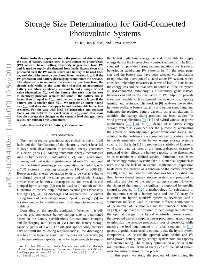
In this section, we formulate the problem of determining thestorage size for grid-connected PV system, as shown in Fig. 1.Solar panels are used to generate electricity, which can be usedto supply loads, e.g., lights, air conditioners, microwaves in a

1Note that solar panels and batteries both operate on DC, while the gridand loads operate on AC. Therefore, DC-to-AC power conversion is necessarywhen connecting solar panels and batteries with the grid andloads. In thispaper, the conversion efficiency is assumed to be1, and conversion devicesare not drawn in Fig. 1.

residential setting. If there is excess electricity, it canbe storedin a battery, or dumped into the grid if the battery is fullycharged. On the other hand, if there is not enough electricity topower the loads, electricity can be drawn from the electric grid.Before formalizing the storage size determination problem, wefirst introduce different components in our setting.

A. Photovoltaic Generation

We use the following equation to calculate the electricitygenerated from solar panels:

Ppv(t) = GHI(t)× S × η , (1)

where GHI (Wm−2) is the global horizontal irradiation at thelocation of solar panels,S (m2) is the total area of solar panels,andη is the solar conversion efficiency of the PV cells. ThePV generation model is a simplified version of the one usedin [15] and does not account for PV panel temperature effects.

B. Electric Grid

Electricity can be drawn from (or dumped into) the grid.We associate costs only with the electricity purchase fromthe grid, and assume that there is no benefit by dumpingelectricity into the grid. The motivation is that, from a gridoperator standpoint, it would be most desirable if PV systemcould just serve the local load and not export to the grid. In agrid with very high renewable penetration, there may be morerenewable production than load. In that case, the energy wouldbe dumped.

We useCgp(t) (¢/kWh) to denote the electricity purchaserate,Pgp(t)(W ) to denote the electricity purchased from thegrid at timet, andPgd(t)(W ) to denote the excess electricitydumped to the grid or curtailed at timet. For simplicity, weassume thatCgp(t) is time independentand has the valueCgp.In other words, there is no difference between the electricitypurchase rates at different time instants.

C. Battery

A battery has the following dynamic:

dEB(t)

dt= PB(t) , (2)

Solar Panel

Electric Grid Battery

Load

Fig. 1. Grid-connected PV system with battery storage and loads.

3

whereEB(t)(Wh) is the amount of electricity stored in thebattery at timet, andPB(t)(W ) is the charging/dischargingrate (more specifically,PB(t) > 0 if the battery is charging,andPB(t) < 0 if the battery is discharging). We impose thefollowing constraints on the battery:

i) At any time, the battery chargeEB(t) should satisfyEBmin ≤ EB(t) ≤ EBmax, whereEBmin is the minimumbattery charge,EBmax is the maximum battery charge,and2 0 < EBmin ≤ EBmax, and

ii) The battery charging/discharging rate should satisfyPBmin ≤ PB(t) ≤ PBmax, wherePBmin < 0, −PBmin isthe maximum battery discharging rate, andPBmax > 0 isthe maximum battery charging rate.

For lead-acid batteries, more complicated models exist (e.g.,a third order model is proposed in [16], [17]).

D. Load

Pload(t)(W ) denotes the load at timet. We do not make ex-plicit assumptions on the load considered in Section III exceptthatPload(t) is a (piecewise) continuous function. Loads couldhave a fixed schedule such as lights and TVs, or a relativelyflexible schedule such as refrigerators and air conditioners.For example, air conditioners can be turned on and off withdifferent schedules as long as the room temperature is within acomfortable range. In Section IV, we consider constant loads,i.e., Pload(t) is independent of timet.

E. Minimization of Electricity Purchase Cost

With all the components introduced earlier, now we canformulate the following problem of minimizing the electricitypurchase cost from the electric grid while guaranteeing thatthe demand from loads are satisfied:

minPB ,Pgp,Pgd

∫ t0+T

t0

CgpPgp(τ)dτ

s.t.Ppv(t) + Pgp(t) = Pgd(t) + PB(t) + Pload(t) , (3)

dEB(t)

dt= PB(t) ,

EBmin ≤ EB(t) ≤ EBmax ,

EB(t0) = EBmin ,

PBmin ≤ PB(t) ≤ PBmax ,

Pgp(t) ≥ 0, Pgd(t) ≥ 0 , (4)

wheret0 is the initial time,T is the time period consideredfor the cost minimization. Eq. (3) is the power balancerequirement for any timet ∈ [t0, t0 + T ]; in other words, thesupply of electricity (either from PV generation, grid purchase,or battery discharging) must meet the demand.

F. Storage Size Determination

Based on Eq. (3), we obtain

Pgp(t) = Pload(t)− Ppv(t) + PB(t) + Pgd(t) .

2Usually,EBmin is chosen to be larger than0 to prevent fast battery aging.For detailed modeling of the aging process, refer to [5].

Then the optimization problem in Eq. (4) can be rewritten as

minPB ,Pgd

∫ t0+T

t0

Cgp(Pload(τ)− Ppv(τ) + PB(τ) + Pgd(τ))dτ

s.t.dEB(t)

dt= PB(t) ,

EBmin ≤ EB(t) ≤ EBmax ,

EB(t0) = EBmin ,

PBmin ≤ PB(t) ≤ PBmax ,

Pgd(t) ≥ 0 .

Now there are two independent variablesPB(t) andPgd(t).To minimize the total electricity purchase cost, we have thefollowing key observations:

(A) If the battery is charging, i.e.,PB(t) > 0 andEB(t) <EBmax, then the charged electricity should only comefrom excess PV generation;

(B) If the battery is discharging, i.e.,PB(t) < 0 andEB(t) > EBmin, then the discharged electricity shouldonly be used to supply loads. In other words, the dumpedelectric powerPgd(t) should only come from excess PVgeneration.

In observation (A), the battery can be charged by grid pur-chased electricity at the current time and be used later onwhen the PV generated electricity is insufficient to meetdemands. However, this incurs a cost at the current time,and the saving of costs by discharging later on is the sameas the cost of charging (or could be less than the cost ofcharging if the discharged electricity gets dumped into thegrid) because the electricity purchase rate is time independent.That is to say, there is no gain in terms of costs by operatingthe battery charging in this way. Therefore, we can restrictthebattery charging to using only PV generated electric power.Inobservation (B), if the battery charge is dumped into the grid,potentially it could increase the total cost since extra electricitymight need to be purchased from the grid to meet the demand.In summary, we have the following rule to operate the batteryand dump electricity to the grid (i.e., restricting the set ofpossible control actions) without increasing the total cost.

Rule 1 Only when there is excess PV generated electricpower and the battery can still be charged, the battery getscharged from the PV generation; only when the load cannotbe met by PV generated electric power and the battery canstill be discharged, the battery gets discharged to supply theload; only when there is excess PV generated electric powerother than supplying both the load and the battery charging,excess PV generated electric power gets dumped into the grid.

With this operating rule, we can further eliminate thevariable Pgd(t) and obtain another equivalent optimizationproblem. On the one hand, ifPload(t)−Ppv(t)+PB(t) < 0, i.e.,the electricity generated from PV is more than the electricityconsumed by the load and charging the battery, we need tochoosePgd(t) > 0 to makePgp(t) = 0 so that the cost isminimized; on the other hand, ifPload(t)−Ppv(t)+PB(t) > 0,i.e., the electricity generated from PV and battery discharging

4

is less than the electricity consumed by the load, we need tochoosePgd(t) = 0 to minimize the electricity purchase costs,and we havePgp(t) = Pload(t) − Ppv(t) + PB(t). Therefore,Pgp(t) can be written as

Pgp(t) = max(0, Pload(t)− Ppv(t) + PB(t)) ,

so that the integrand is minimized at each time.Let

x(t) = EB(t)−EBmax+ EBmin

2,

u(t) = PB(t), and

Emax =EBmax− EBmin

2.

Note that2Emax = EBmax − EBmin is the net (usable) batterycapacity, which is the amount of electricity that can be storedin the battery. Then the optimization problem can be rewrittenas

J = minu

∫ t0+T

t0

Cgpmax(0, Pload(τ) − Ppv(τ) + u(τ))dτ

s.t.dx(t)

dt= u(t) ,

|x(t)| ≤ Emax ,

x(t0) = −Emax ,

PBmin ≤ u(t) ≤ PBmax . (5)

Now it is clear that onlyu(t) (or equivalently,PB(t)) is anindependent variable. As argued previously, we can restrictu(t) to satisfying Rule 1 without increasing the minimum costJ . We define the set of feasible controls (denoted asUfeasible)as controls that satisfy the constraintPBmin ≤ u(t) ≤ PBmax

and do not violate Rule 1.If we fix the parameterst0, T, PBmin, and PBmax, J is a

function ofEmax, which is denoted asJ(Emax). If Emax = 0,thenu(t) = 0, andJ reaches the largest value

Jmax =

∫ t0+T

t0

Cgpmax(0, Pload(τ) − Ppv(τ))dτ . (6)

If we increaseEmax, intuitively J will decrease (though maynot strictly decrease) because the battery can be utilized tostore extra electricity generated from PV to be potentiallyused later on when the load exceeds the PV generation andthe battery discharging. This is justified in the followingproposition.

Proposition 1 Given the optimization problem in Eq. (5), ifE1

max < E2max, thenJ(E1

max) ≥ J(E2max).

Proof: Given E1max, suppose a feasible controlu1(t)

achieves the minimum electricity purchase costJ(E1max) and

the corresponding statex is x1(t). Since |x1(t)| ≤ E1max <

E2max, u1(t) is also a feasible control for problem (5) with

the state constraintE2max and satisfying Rule 1, and results in

the costJ(E1max). SinceJ(E2

max) is the minimal cost over theset of all feasible controls which includeu1(t), we must haveJ(E1

max) ≥ J(E2max).

In other words,J is monotonically decreasing with respectto the parameterEmax, and is lower bounded by0. We are

interested in finding the smallest value ofEmax (denoted asEc

max) such thatJ remains the same for anyEmax ≥ Ecmax,

and call it the storage size determination problem.

Problem 1 (Storage Size Determination) Given the opti-mization problem in Eq. (5) with fixedt0, T, PBmin andPBmax,determine a critical valueEc

max ≥ 0 such that∀Emax < Ecmax,

J(Emax) > J(Ecmax), and∀Emax ≥ Ec

max, J(Emax) = J(Ecmax).

Remark 1 In the storage size determination problem, we fixthe charging and discharging rate of the battery while varyingthe battery capacity. This is reasonable if the battery is chargedwith a fixed charger, which uses a constant charging voltagebut can change the charging current within a certain limit.In practice, the charging and discharging rates could scalewith Emax, which results in challenging problems to solve andrequires further study. �

Note that the critical valueEcmax is unique as shown below.

Proposition 2 Given the optimization problem in Eq. (5) withfixed t0, T, PBmin andPBmax, Ec

max is unique.

Proof: We prove it via contradiction. SupposeEcmax is

not unique. In other words, there are two different criticalvaluesEc1

max and Ec2max. Without loss of generality, suppose

Ec1max < Ec2

max. By definition, J(Ec1max) > J(Ec2

max) becauseEc2

max is a critical value, whileJ(Ec1max) = J(Ec2

max) becauseEc1

max is a critical value. A contradiction. Therefore, we musthaveEc1

max = Ec2max.

Remark 2 One idea to calculate the critical valueEcmax is

that we first obtain an explicit expression for the functionJ(Emax) by solving the optimization problem in Eq. (5) andthen solve forEc

max based on the functionJ . However, theoptimization problem in Eq. (5) is difficult to solve due to thestate constraint|x(t)| ≤ Emax and the fact that it is hard toobtain analytical expressions forPload(t) andPpv(t) in reality.Even though it might be possible to find the optimal controlusing the minimum principle [18], it is still hard to get anexplicit expression for the cost functionJ . Instead, in the nextsection, we first focus on bounding the critical valueEc

max ingeneral, and then study the problem for specific scenarios inSection IV. �

III. U PPERBOUND ON Ecmax

In this section, we first identify necessary assumptions toensure a nonzeroEc

max, then propose an upper bound onEcmax,

and finally show that the upper bound is tight for certainscenarios.

Proposition 3 Given the optimization problem in Eq. (5) withfixed t0, T, PBmin andPBmax, Ec

max = 0 if any of the followingconditions holds:(i) ∀t ∈ [t0, t0 + T ], Ppv(t)− Pload(t) ≤ 0,(ii) ∀t ∈ [t0, t0 + T ], Ppv(t)− Pload(t) ≥ 0,

(iii) ∀t1 ∈ S1, ∀t2 ∈ S2, t2 < t1, where

S1 :={t ∈ [t0, t0 + T ] | Ppv(t)− Pload(t) > 0} , (7)

S2 :={t ∈ [t0, t0 + T ] | Pload(t)− Ppv(t) > 0} . (8)

5

Proof: Condition (i) holds. Since ∀t ∈ [t0, t0 + T ],Ppv(t) − Pload(t) ≤ 0, we havePload(t) − Ppv(t) ≥ 0.Denote the integrand inJ of Eq. (5) asα, i.e., α(t) =Cgpmax(0, Pload(t)−Ppv(t) + u(t)). If Pload(t)−Ppv(t) = 0,then we could chooseu(t) = 0 to makeα to be0. If Pload(t)−Ppv(t) > 0, we could choosePpv(t) − Pload(t) ≤ u(t) < 0 todecreaseα, i.e., by discharging the battery. However, sincex(t0) = −Emax, there is no electricity stored in the batteryat the initial time. To be able to discharge the battery, it musthave been charged previously. Following Rule 1, the electricitystored in the battery should only come from excess PV gener-ation. However, there is no excess PV generation at any timebecause∀t ∈ [t0, t0+T ], Ppv(t)−Pload(t) ≤ 0. Therefore, thecost is not reduced by choosingPpv(t)−Pload(t) ≤ u(t) < 0.In other words,u can be chosen to be0. In both cases,u(t)can be0 for any t ∈ [t0, t0 + T ] without increasing the cost,and thus, no battery is necessary. Therefore,Ec

max = 0.Condition (ii) holds. Since ∀t ∈ [t0, t0 + T ], Ppv(t) −Pload(t) ≥ 0, we havePload(t) − Ppv(t) ≤ 0. Denote theintegrand in J as α, i.e., α(t) = Cgpmax(0, Pload(t) −Ppv(t) + u(t)). If Pload(t) − Ppv(t) ≤ 0, we could chooseu(t) = 0, and thenα = max(0, Pload(t) − Ppv(t) + u(t)) =max(0, Pload(t) − Ppv(t)) = 0. Sinceu(t) can be0 for anyt ∈ [t0, t0 + T ] without increasing the cost, no battery isnecessary. Therefore,Ec

max = 0.Condition (iii) holds. S1 is the set of time instants at whichthere is extra amount of electric power that is generated fromPV after supplying the load, whileS2 is the set of time instantsat which the PV generated power is insufficient to supply theload. According to Rule 1, at timet, the battery could getcharged only ift ∈ S1, and could get discharged only ift ∈S2. If ∀t1 ∈ S1, ∀t2 ∈ S2, t2 < t1 implies that even if theextra amount of electricity generated from PV is stored in abattery, there is no way to use the stored electricity to supplythe load. This is because the electricity is stored after thetimeinstants at which battery discharging can be used to strictlydecrease the cost and initially there is no electricity stored inthe battery. Therefore, the costs are the same for the scenariowith battery and the scenario without battery, andEc

max = 0.

Remark 3 The intuition of condition (i) in Proposition 3 isthat if ∀t ∈ [t0, t0 + T ], Ppv(t) − Pload(t) ≤ 0, no extra elec-tricity is generated from PV and can be stored in the batteryto strictly reduce the cost. The intuition of condition (ii)inProposition 3 is that if∀t ∈ [t0, t0+T ], Ppv(t)−Pload(t) ≥ 0,the electricity generated from PV alone is enough to satisfytheload all the time, and extra electricity can be simply dumpedto the grid. Note thatJmax = 0 for this case. As defined incondition (iii), S1 ∩ S2 = ∅ because it is impossible to haveboth Ppv(t) − Pload(t) > 0 andPload(t) − Ppv(t) > 0 at thesame time for any timet. �

Based on the result in Proposition 3, we impose the follow-ing assumption on Problem 1 to make use of the battery.

Assumption 1 There existst1 andt2 for t1, t2 ∈ [t0, t0+T ],such thatt1 < t2, Ppv(t1) − Pload(t1) > 0 and Ppv(t2) −Pload(t2) < 0.

Remark 4 Ppv(t1) − Pload(t1) > 0 implies that at timet1there is excess electric power available from PV.Ppv(t2) −Pload(t2) < 0 implies that at timet2 the electric power fromPV is not sufficient for the load. Ift1 < t2, the electricitystored in the battery at timet1 can be discharged to power theload at timet2 to strictly reduce the cost. �

Proposition 4 Given the optimization problem in Eq. (5) withfixed t0, T, PBmin andPBmax under Assumption 1,0 < Ec

max ≤min(A,B)

2 , where

A =

∫ t0+T

t0

min(PBmax,max(0, Ppv(t)− Pload(t)))dt , (9)

and

B =

∫ t0+T

t0

min(−PBmin,max(0, Pload(t)−Ppv(t)))dt . (10)

Proof: It can be shown, via contradiction, that underAssumption 1,A > 0 and B > 0, which imply thatmin(A,B)

2 > 0.We showEc

max > 0 via contradiction. SinceEcmax ≥ 0,

we need exclude the caseEcmax = 0. SupposeEc

max = 0. Ifwe chooseEmax > Ec

max = 0, J(Emax) < J(Ecmax) because

under Assumption 1 a battery can store the extra PV generatedelectricity first and then use it later on to strictly reduce thecost compared with the case without a battery (i.e., the casewith Emax = 0). A contradiction to the definition ofEc

max.To showEc

max ≤ min(A,B)2 , it is sufficient to show that if

Emax ≥ min(A,B)2 , then J(Emax) = J(min(A,B)

2 ). There aretwo cases depending onA andB:

• A ≤ B. Then min(A,B) = A. At time t,max(0, Ppv(t) − Pload(t)) is the extra amount of electricpower that is generated from PV after supplying theload, andmin(PBmax,max(0, Ppv(t) − Pload(t))) is theextra amount of electric power that is generated fromPV after supplying the load and can be stored in abattery subject to the maximum charging rate. ThenA =

∫ t0+T

t0min(PBmax,max(0, Ppv(t) − Pload(t)))dt is

the maximum total amount of extra electricity that canbe stored in a battery while taking the battery chargingrate into account. Even if2Emax ≥ A, i.e., Emax ≥ A

2 ,the amount of electricity that can be stored in the batterycannot exceedA. Therefore, any control that is feasiblewith |x(t)| ≤ Emax is also feasible with|x(t)| ≤ A

2 .Therefore,J(Emax) = J(A2 ) = J(min(A,B)

2 );• A > B. Then min(A,B) = B. At time t,

max(0, Pload(t)−Ppv(t)) is the amount of electric powerthat is necessary to satisfy the load (and could besupplied by either battery power or grid purchase), andmin(−PBmin,max(0, Pload(t) − Ppv(t))) is the amountof electric power that can potentially be dischargedfrom a battery to supply the load subject to the max-imum discharging rate (in other words, ifPload(t) −Ppv(t) > −PBmin, electricity must be purchased from thegrid). ThenB =

∫ t0+T

t0min(−PBmin,max(0, Pload(t) −

Ppv(t)))dt is the maximum total amount of electricitythat is necessary to be discharged from the battery to

6

satisfy the load while taking the battery discharging rateinto account. When2Emax ≥ B, i.e., Emax ≥ B

2 , theamount of electricity that can be charged can exceedB becauseA > B; however, the amount of electricitythat is strictly necessary to be and, at the same time,can be discharged does not exceedB. In other words, ifthe stored electricity in the battery exceeds this amountB, the extra electricity cannot help reduce the costbecause it either cannot be discharged or is not necessary.Therefore, any control that minimizes the total cost withthe battery capacity beingB also minimizes the totalcost with the battery capacity being2Emax. Therefore,J(Emax) = J(B2 ) = J(min(A,B)

2 ).

Remark 5 Note that if ∀t ∈ [t0, t0 + T ] we havePpv(t) −Pload(t) ≤ 0, then A = 0 following Eq. (9); therefore, theupper bound forEc

max in Proposition 4 becomes0, whichimplies that Ec

max = 0. If ∀t ∈ [t0, t0 + T ] we havePpv(t) − Pload(t) ≥ 0, then B = 0 following Eq. (10);therefore, the upper bound forEc

max in Proposition 4 becomes0, which implies thatEc

max = 0. Both results are consistentwith the results in Proposition 3. �

Proposition 5 Given the optimization problem in Eq. (5) withfixed t0, T, PBmin andPBmax under Assumption 1, if∀t1 ∈ S1,∀t2 ∈ S2, t1 < t2, thenEc

max =min(A,B)

2 , whereS1 (or S2,A, B, respectively) is defined in Eq. (7) (or (8), (9), (10),respectively). In addition, ifEmax is chosen to bemin(A,B)

2 ,x(t0+T ) = −Emax (i.e., no battery charge left at timet0+T ).

Proof: From Proposition 4, we haveEcmax ≤ min(A,B)

2 .To proveEc

max = min(A,B)2 , we show thatEc

max <min(A,B)

2

is impossible via contradiction. SupposeEcmax <

min(A,B)2 . If

∀t1 ∈ S1, ∀t2 ∈ S2, t1 < t2, then during the time interval[t0, t0 + T ], the battery is first charged, and then dischargedfollowing Rule 1. In other words, there is no charging afterdischarging. There are two cases depending onA andB:

• A ≤ B. In this case,Ecmax <

A2 , i.e., 2Ec

max < A. If thebattery capacity is2Ec

max, then the amount of electricityA− 2Ec

max > 0 (which is generated from PV) cannot bestored in the battery. If we choose the battery capacity tobeA, this extra amount can be stored and used later onto strictly decrease the cost becauseA ≤ B. Therefore,J(A2 ) < J(Ec

max). A contradiction to the definition ofEc

max. In this case, ifEmax is chosen to beA2 , then thebattery is first charged withA amount of electricity, andthen completely discharged before (or at)t0+T becauseA ≤ B. Therefore, we havex(t0 + T ) = −Emax.

• A > B. In this case,Ecmax < B

2 , i.e., 2Ecmax < B. If

the battery capacity is2Ecmax, at most2Ec

max < B < A

amount of PV generated electricity can be stored in thebattery. Therefore, the amount of electricityB−2Ec

max >

0 must be purchased from the grid to supply the load.If we choose the battery capacity to beB, the amountof electricity B − 2Ec

max purchased from the grid canbe provided by the battery because the battery can becharged with the amount of electricityB (sinceA > B),

and thus the cost can be strictly decreased. Therefore,J(B2 ) < J(Ec

max). A contradiction to the definition ofEc

max. In this case, ifEmax is chosen to beB2 , then thebattery is first charged withB amount of electricity (thatis to say, not all extra electricity generated from PV isstored in the battery sinceA > B), and then completelydischarged at timet0+T . Therefore, we also havex(t0+T ) = −Emax.

IV. I DEAL PV GENERATION AND CONSTANT LOAD

In this section, we study how to obtain the critical value forthe scenario in which the PV generation is ideal and the load isconstant. Ideal PV generation occurs on clear days; for a typi-cal south-facing PV array on a clear day, the PV output is zerobefore about sunrise, rises continuously and monotonically toits maximum around solar noon, then decreases continuouslyand monotonically to zero around sunset, as shown in Fig. 2(a).In other words, there is essentially no short time fluctuation(at the scale of seconds to minutes) due to atmospheric effectssuch as clouds or precipitation. By constant load, we meanPload(t) is a constant fort ∈ [t0, t0 + T ]. A typical constantload is plotted in Fig. 2(b). To further simplify the problem,we assume thatt0 is 0000 h Local Standard Time (LST), andT = t0 + k × 24(h) wherek is a nonnegative integer, i.e.,Tis a duration of multiple days. Fig. 2 plots the PV generationand the constant load forT = 24(h). Now we can formalizethese conditions in the following assumption.

Assumption 2 The initial time t0 is 0000 h LST, T = k ×24(h) wherek is a nonnegative integer,Ppv(t) is periodic ona timescale of24 hours, and satisfies the following propertyfor t ∈ [0, 24(h)]: there exist three time instants0 < tsunrise<

tmax < tsunset< 24(h) such that

• Ppv(t) = 0 for t ∈ [0, tsunrise] ∪ [tsunset, 24(h)];• Ppv(t) is continuous and strictly increasing fort ∈

[tsunrise, tmax];• Ppv(t) achieves its maximumPmax

pv at tmax;• Ppv(t) is continuous and strictly decreasing fort ∈

[tmax, tsunset],

and Pload(t) = Pload for t ∈ [t0, t0 + T ], wherePload is aconstant satisfying0 < Pload < Pmax

pv .

It can be verified that Assumption 2 implies Assumption 1.

Proposition 6 Given the optimization problem in Eq. (5) withfixed t0, T, PBmin and PBmax under Assumption 2 andT =24(h), Ec

max =min(A1,B1)

2 , where

A1 =

∫ t2

t1

min(PBmax,max(0, Ppv(t)− Pload))dt ,

and

B1 =

∫ 24

t2

min(−PBmin,max(0, Pload− Ppv(t)))dt ,

in which t1 < t2 andPpv(t1) = Ppv(t2) = Pload.

Proof: Due to Assumption 2,Pload(t) intersects withPpv(t) at two time instants forT = 24(h); the smaller time

7

replacements

0 tsunrise tsunset 24

Ppv(W )

t(h)

(a) Ideal PV generation for a clear day.

0 24

Ppv(W )

t(h)

(b) Constant load.

Fig. 2. Ideal PV generation and constant load.

instant is denoted ast1, and the larger is denoted ast2, asshown in Fig. 3. It can be verified thatPpv(t) > Pload fort ∈ (t1, t2) and Ppv(t) < Pload for t ∈ [0, t1) ∪ (t2, 24]following Assumption 2. Fort ∈ [0, t1), a battery couldonly get discharged following Rule 1; however, it cannot bedischarged becausex(0) = −Emax. Therefore,u(t) can be0 while achieving the lowest cost for the time period[0, t1).Then the objective function of the optimization problem inEq. (5) can be rewritten as

J = min

∫ 24

0

Cgpmax(0, Pload− Ppv(τ) + u(τ))dτ

= J0 + J1 ,

whereJ0 =∫ t1

0 Cgp(Pload− Ppv(τ))dτ is a constant which isindependent of the controlu, and

J1 = min

∫ 24

t1

Cgpmax(0, Pload− Ppv(τ) + u(τ))dτ .

In other words, the optimization problem is essentially thesame as minimizingJ1 for t ∈ [t1, 24]; accordingly, the criticalvalueEc

max will be the same since the battery is not used forthe time interval[0, t1]. For the optimization problem withthe cost functionJ1 under Assumption 2,S1 = (t1, t2) andS2 = (t2, 24) according to Eqs. (7) and (8). Since∀t′1 ∈ S1,∀t′2 ∈ S2, t′1 < t2 < t′2, the conditions in Proposition 5 aresatisfied. Thus, we haveEc

max =min(A,B)

2 , where

A =

∫ 24

t1

min(PBmax,max(0, Ppv(t)− Pload))dt

=

∫ t2

t1

min(PBmax,max(0, Ppv(t)− Pload))dt,

0 t1 t2 24

Ppv(W )

t(h)

PBmax

−PBmin

A1

B1

Fig. 3. PV generation and load, wherePBmax (or −PBmin) is the maximumcharging (or discharging) rate, andA1, B1, t1, t2 are defined in Proposition 6.

which is essentiallyA1, and

B =

∫ 24

t1

min(−PBmin,max(0, Pload− Ppv(t)))dt

=

∫ 24

t2

min(−PBmin,max(0, Pload− Ppv(t)))dt ,

which is essentiallyB1. Thus the result holds.

Remark 6 A1 andB1 in Proposition 6 are shown in Fig. 3. Inwords,A1 is the amount of extra PV generated electricity thatcan be stored in a battery, andB1 is the amount of electricitythat is necessary to supply the loadand can be provided bybattery discharging. Note thatt1 and t2 depend on the valueof Pload. To eliminate this dependency, we can rewriteA1 as

A1 =

∫ 24

0

min(PBmax,max(0, Ppv(t)− Pload))dt , (11)

and rewriteB1 as

B1 =

∫ 24

tmax

min(−PBmin,max(0, Pload− Ppv(t)))dt , (12)

wheretmax is defined in Assumption 2. �

Remark 7 If the PV generation is not ideal, i.e., there arefluctuations due to clouds or precipitation, theEc

max value inProposition 6 based on ideal PV generation naturally servesas an upper bound onEc

max for the case with the non-idealPV generation. Similarly, if the load varies with time but isbounded by a constantPload, theEc

max values in Proposition 6based on the constant loadPload naturally serves as an upperbound onEc

max for the case with the time varying load. �

Now we examine howEcmax changes asPload varies from0

to Pmaxpv .

Proposition 7 Given the optimization problem in Eq. (5) withfixed t0, T, PBmin and PBmax under Assumption 2 andT =24(h), then

a) there exists a unique critical value ofPload ∈ (0, pmaxpv )

(denoted asP cload) such thatEc

max achieves its maximum;b) if Pload increases from0 to P c

load, Ecmax increases contin-

uously and monotonically from0 to its maximum;c) if Pload increases fromP c

load to Pmaxpv , Ec

max decreasescontinuously and monotonically from its maximum to0.

8

Proof: Let f := A1 −B1, whereA1 andB1 are definedin Eqs. (11) and (12). Note thatf is a function ofPload. IfPload = 0, then

A1 =

∫ 24

0

min(PBmax,max(0, Ppv(t)))dt > 0 ,

according to Eq. (11), and

B1 =

∫ 24

tmax

min(−PBmin,max(0,−Ppv(t)))dt = 0 ,

according to Eq. (12). Therefore,f(0) = A1(0)−B1(0) > 0.If Pload = Pmax

pv , then

A1 =

∫ 24

0

min(PBmax,max(0, Ppv(t)− Pmaxpv ))dt = 0,

and

B1 =

∫ 24

tmax

min(−PBmin,max(0, Pmaxpv − Ppv(t)))dt > 0 .

Therefore,f(Pmaxpv ) = A1(P

maxpv )−B1(P

maxpv ) < 0. In addition,

sincef is an integral of a continuous function ofPload, f isdifferentiable with respect toPload, and the derivative is givenas

df

dPload=

dA1

dPload−

dB1

dPload.

Since forPload ∈ (0, Pmaxpv ),

dA1

dPload=

∫ 24

0

(−1)× I{0 < Ppv(t)− Pload ≤ PBmax}dt

< 0 ,

and

dB1

dPload=

∫ 24

tmax

1× I{0 < Pload− Ppv(t) ≤ −PBmin}dt

> 0 ,

we have dfdPload

< 0, whereI{0 < Ppv(t) − Pload ≤ PBmax} isthe indicator function (i.e., if0 < Ppv(t)− Pload ≤ PBmax, thefunction has value1, 0 otherwise). Therefore,f is continuousand strictly decreasing forPload ∈ [0, Pmax

pv ]. Sincef(0) > 0andf(Pmax

pv ) < 0, there is one and only one value ofPload suchthatf is 0. We denote this value asP c

load and haveA1(Pcload) =

B1(Pcload).

If Pload ∈ [0, P cload), f > 0, i.e., A1 > B1. Therefore,

Ecmax = B1

2 . Since dB1

dPload> 0, Ec

max increases continuously(sinceB1 is differentiable with respect toPload) and mono-tonically from 0 to the valueB1(P

c

load)2 . On the other hand,

if Pload ∈ (P cload, P

maxpv ], f < 0, i.e., A1 < B1. Therefore,

Ecmax = A1

2 . Since dA1

dPload< 0, Ec

max decreases continuously(sinceA1 is differentiable with respect toPload) and mono-tonically from the valueA1(P

c

load)2 =

B1(Pc

load)2 to 0. Therefore,

Ecmax achieves its maximum atP c

load. This completes the proof.

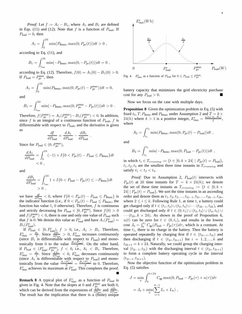
Remark 8 A typical plot of Ecmax as a function ofPload is

given in Fig. 4. Note that the slopes at0 andPmaxpv are both0,

which can be derived from the expressions ofdA1

dPloadand dB1

dPload.

The result has the implication that there is a (finite) unique

0 P cload Pmax

pv Pload(W )

Ecmax(Wh)

B1

2A1

2

Fig. 4. Ecmax as a function ofPload for 0 ≤ Pload ≤ Pmax

pv .

battery capacity that minimizes the grid electricity purchasecost for anyPload > 0. �

Now we focus on the case with multiple days.

Proposition 8 Given the optimization problem in Eq. (5) withfixed t0, T, PBmin andPBmax under Assumption 2 andT = k×24(h) wherek > 1 is a positive integer,Ec

max =min(A2,B2)

2 ,where

A2 =

∫ t2

t1

min(PBmax,max(0, Ppv(t)− Pload))dt ,

and

B2 =

∫ t3

t2

min(−PBmin,max(0, Pload− Ppv(t)))dt ,

in which ti ∈ Tcrossing := {t ∈ [0, k × 24] | Ppv(t) = Pload},t1, t2, t3 are the smallest three time instants inTcrossing andsatisfy t1 < t2 < t3.

Proof: Due to Assumption 2,Pload(t) intersects withPpv(t) at 2k time instants forT = k × 24(h); we denotethe set of these time instants asTcrossing := {t ∈ [0, k ×24] | Ppv(t) = Pload}. We sort the time instants in an ascendingorder and denote them ast1, t2, t3, ..., t2i−1, t2i, ..., t2k−1, t2k,where2 ≤ i ≤ k. Following Rule 1, at timet, a battery couldget charged only ift ∈ (t1, t2)∪ (t3, t4)∪· · · (t2k−1, t2k), andcould get discharged only ift ∈ (0, t1) ∪ (t2, t3) ∪ (t4, t5) ∪· · · (t2k, k × 24). As shown in the proof of Proposition 6,u(t) can be zero fort ∈ (0, t1), and results in the lowestcostJ0 =

∫ t1

0Cgp(Pload− Ppv(τ))dτ , which is a constant. At

time t1, there is no charge in the battery. Then the battery isoperated repeatedly by charging first ift ∈ (t2i−1, t2i) andthen discharging ift ∈ (t2i, t2i+1) for i = 1, 2, ..., k andt2k+1 = k× 24. Naturally, we could group the charging inter-val (t2i−1, t2i) with the discharging intervalt ∈ (t2i, t2i+1)to form a complete battery operating cycle in the interval(t2i−1, t2i+1).

Now the objective function of the optimization problem inEq. (5) satisfies

J = minu

∫ k×24

0

Cgpmax(0, Pload− Ppv(τ) + u(τ))dτ

= J0 +minu

(

k−1∑i=1

Li + Lk) ,

9

where

Li =

∫ t2i+1

t2i−1

Cgpmax(0, Pload− Ppv(τ) + u(τ))dτ ,

for i = 1, 2, ..., k − 1, and

Lk =

∫ t2k+1

t2k−1

Cgpmax(0, Pload− Ppv(τ) + u(τ))dτ .

Note that given a certainEmax, if the battery charge at theend of the first battery operating cycle is larger than0 (i.e.,x(t3) > −Emax), thenEmax > Ec

max. This can be argued asfollows. If the battery charge at the end of the first cycleis larger than0 (this also implies that the battery charge atthe end of the ith cycle is also larger than0 due to periodicPV generations and loads), i.e., there is more PV generationthan demand in the time interval(t1, t3), thenEmax can bestrictly reduced to a smaller capacity so thatx(t3) = −Emax

without increasing the electricity purchase cost in the interval(t1, t3). Due to periodicity of the PV generation and the load,the smallerEmax can be used for the interval(t2i−1, t2i+1)for i = 2, ..., k− 1 without increasing the electricity purchasecost. Therefore, thisEmax must be larger thanEc

max. In otherwords, ifEc

max is used, thenx(t2i+1) for i = 1, 2, ..., k−1 hasto be−Ec

max, i.e., no charge left at the end of each operatingcycle. Now we only considerEmax such that at the end ofeach operating cyclex(t2i+1) = −Emax for i = 1, 2, ..., k− 1(necessarily,Ec

max is smaller than or equal to any suchEmax).For suchEmax, the control actions for each operating cycleare completely decoupled3. Therefore, the total costJ can berewritten as

J = J0 +

k−1∑i=1

Ji + Jk ,

whereJi = minu Li for i = 1, 2, ..., k.Now we focus onJ1. For the optimization problem with

the cost functionJ1 under Assumption 2,S1 = (t1, t2) andS2 = (t2, t3) according to Eqs. (7) and (8). Since∀t′1 ∈ S1,∀t′2 ∈ S2, t′1 < t2 < t′2, the conditions in Proposition 5 aresatisfied. Thus, we haveEc

max(1) =min(A,B)

2 , whereEcmax(1)

is theEcmax when we only consider the cost functionJ1,

A =

∫ t3

t1

min(PBmax,max(0, Ppv(t)− Pload))dt

=

∫ t2

t1

min(PBmax,max(0, Ppv(t)− Pload))dt ,

which is essentiallyA2, and

B =

∫ t3

t1

min(−PBmin,max(0, Pload− Ppv(t)))dt

=

∫ t3

t2

min(−PBmin,max(0, Pload− Ppv(t)))dt ,

3Note that the control action fort ∈ (t2i−1, t2i) and the control actionfor t ∈ (t2i, t2i+1) for i = 1, 2, ..., k are coupled in the sense that batterycan not be discharged if at timet2i there is no charge in the battery. Ingeneral, the control action fort ∈ (t2i, t2i+1) and the control action fort ∈ (t2i+1, t2i+2) for i = 1, k − 1 can also be coupled if at timet2i+1

there is extra charge left in the battery because the extra charge will affectthe charging action in the intervalt ∈ (t2i+1, t2i+2). Here, there is no suchcoupling for the latter case when we restrictEmax so that at the end of eachoperating cycle there is no charge left.

which is essentiallyB2. Thus we haveEcmax(1) =

min(A2,B2)2 .

Based on Proposition 5, we also know thatx(t3) = −Ecmax(1).

Thus, thisEcmax(1) satisfies the requirement that at the end of

the operating cycle there is no charge left.For the cost functionJ2, the optimization problem is

essentially the same as the problem with the cost functionJ1 because

• Ppv(t) = Ppv(t − 24) for t ∈ [t3, t5] becausePpv(t) isperiodic with period24 hours. Note thatt−24 ∈ [t1, t3];

• Pload(t) is a constant; and• there is no charge left att3.

In other words, there is no difference between the optimizationproblem with the cost functionJ2 and the one withJ1 otherthan the shifting of timet by 24 hours. Therefore, theEc

max(2)will be the same asEc

max(1). The same reasoning applies tothe optimization problem with the cost functionJi for i =3, ..., k − 1. Therefore, we haveEc

max(i) = Ecmax(1) for i =

2, ..., k − 1.For the optimization problemJk, there is no charge left

at time 2k − 1. This problem is essentially the same as theproblem studied in the proof of Proposition 6 with the costfunction J1 except the shifting of timet by (k − 1) × 24

hours. The solutionEcmax(k) is given asmin(Ak,Bk)

2 , where

Ak =

∫ t2k

t2k−1

min(PBmax,max(0, Ppv(t)− Pload))dt ,

and

Bk =

∫ t2k+1

t2k

min(−PBmin,max(0, Pload− Ppv(t)))dt .

Note thatAk = A2, andBk < B2. If we chooseEmax =min(A2,B2)

2 which is larger than or equal toEcmax(k), we have

Jk(Emax) = Jk(Ecmax(k)).

Now we claim thatEcmax when considering the cost function

J is exactly min(A2,B2)2 . If we chooseEmax <

min(A2,B2)2 ,

then J(Emax) > J(min(A2,B2)2 ) by an argument similar to

the one in Proposition 5. On the other hand, if we chooseEmax ≥ min(A2,B2)

2 , then J(Emax) = J(min(A2,B2)2 ). There-

fore,Ecmax to the optimization problem with the cost function

J is min(A2,B2)2 .

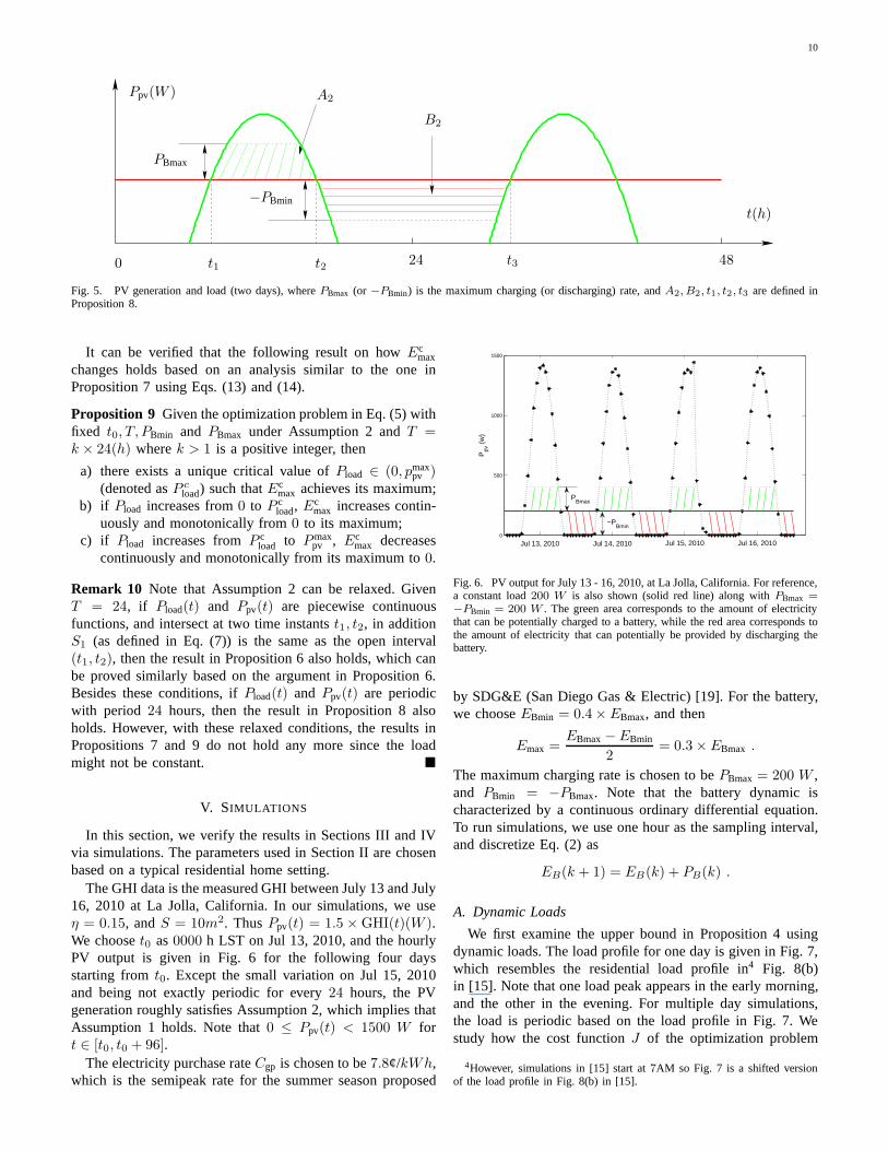
Remark 9 A2 andB2 in Proposition 8 are shown in Fig. 5.In words,A2 is the amount of extra PV generated electricitythat can be stored in a battery in the time interval[t1, t3], andB2 is the amount of electricity that is necessary to supply theload and can be provided by battery discharging in the timeinterval [t1, t3]. Note thatt1 and t3 depend on the value ofPload. To eliminate this dependency, we can rewriteA2 as

A2 =

∫ 24

0

min(PBmax,max(0, Ppv(t)− Pload))dt , (13)

and rewriteB2 as

B2 =

∫ tmax+24

tmax

min(−PBmin,max(0, Pload−Ppv(t)))dt , (14)

wheretmax is defined in Assumption 2. �

10

0 t1 t2 24

Ppv(W )

t(h)

PBmax

−PBmin

A2

B2

t3 48

Fig. 5. PV generation and load (two days), wherePBmax (or −PBmin) is the maximum charging (or discharging) rate, andA2, B2, t1, t2, t3 are defined inProposition 8.

It can be verified that the following result on howEcmax

changes holds based on an analysis similar to the one inProposition 7 using Eqs. (13) and (14).

Proposition 9 Given the optimization problem in Eq. (5) withfixed t0, T, PBmin and PBmax under Assumption 2 andT =k × 24(h) wherek > 1 is a positive integer, then

a) there exists a unique critical value ofPload ∈ (0, pmaxpv )

(denoted asP cload) such thatEc

max achieves its maximum;b) if Pload increases from0 to P c

load, Ecmax increases contin-

uously and monotonically from0 to its maximum;c) if Pload increases fromP c

load to Pmaxpv , Ec

max decreasescontinuously and monotonically from its maximum to0.

Remark 10 Note that Assumption 2 can be relaxed. GivenT = 24, if Pload(t) and Ppv(t) are piecewise continuousfunctions, and intersect at two time instantst1, t2, in additionS1 (as defined in Eq. (7)) is the same as the open interval(t1, t2), then the result in Proposition 6 also holds, which canbe proved similarly based on the argument in Proposition 6.Besides these conditions, ifPload(t) and Ppv(t) are periodicwith period 24 hours, then the result in Proposition 8 alsoholds. However, with these relaxed conditions, the resultsinPropositions 7 and 9 do not hold any more since the loadmight not be constant. �

V. SIMULATIONS

In this section, we verify the results in Sections III and IVvia simulations. The parameters used in Section II are chosenbased on a typical residential home setting.

The GHI data is the measured GHI between July 13 and July16, 2010 at La Jolla, California. In our simulations, we useη = 0.15, andS = 10m2. ThusPpv(t) = 1.5 ×GHI(t)(W ).We chooset0 as0000 h LST on Jul 13, 2010, and the hourlyPV output is given in Fig. 6 for the following four daysstarting fromt0. Except the small variation on Jul 15, 2010and being not exactly periodic for every24 hours, the PVgeneration roughly satisfies Assumption 2, which implies thatAssumption 1 holds. Note that0 ≤ Ppv(t) < 1500 W fort ∈ [t0, t0 + 96].

The electricity purchase rateCgp is chosen to be7.8¢/kWh,which is the semipeak rate for the summer season proposed

0

500

1000

1500

Jul 13, 2010 Jul 14, 2010 Jul 15, 2010 Jul 16, 2010

Ppv

(w

)

PBmax

−PBmin

Fig. 6. PV output for July 13 - 16, 2010, at La Jolla, California. For reference,a constant load200 W is also shown (solid red line) along withPBmax =−PBmin = 200 W . The green area corresponds to the amount of electricitythat can be potentially charged to a battery, while the red area corresponds tothe amount of electricity that can potentially be provided by discharging thebattery.

by SDG&E (San Diego Gas & Electric) [19]. For the battery,we chooseEBmin = 0.4× EBmax, and then

Emax =EBmax− EBmin

2= 0.3× EBmax .

The maximum charging rate is chosen to bePBmax = 200 W ,and PBmin = −PBmax. Note that the battery dynamic ischaracterized by a continuous ordinary differential equation.To run simulations, we use one hour as the sampling interval,and discretize Eq. (2) as

EB(k + 1) = EB(k) + PB(k) .

A. Dynamic Loads

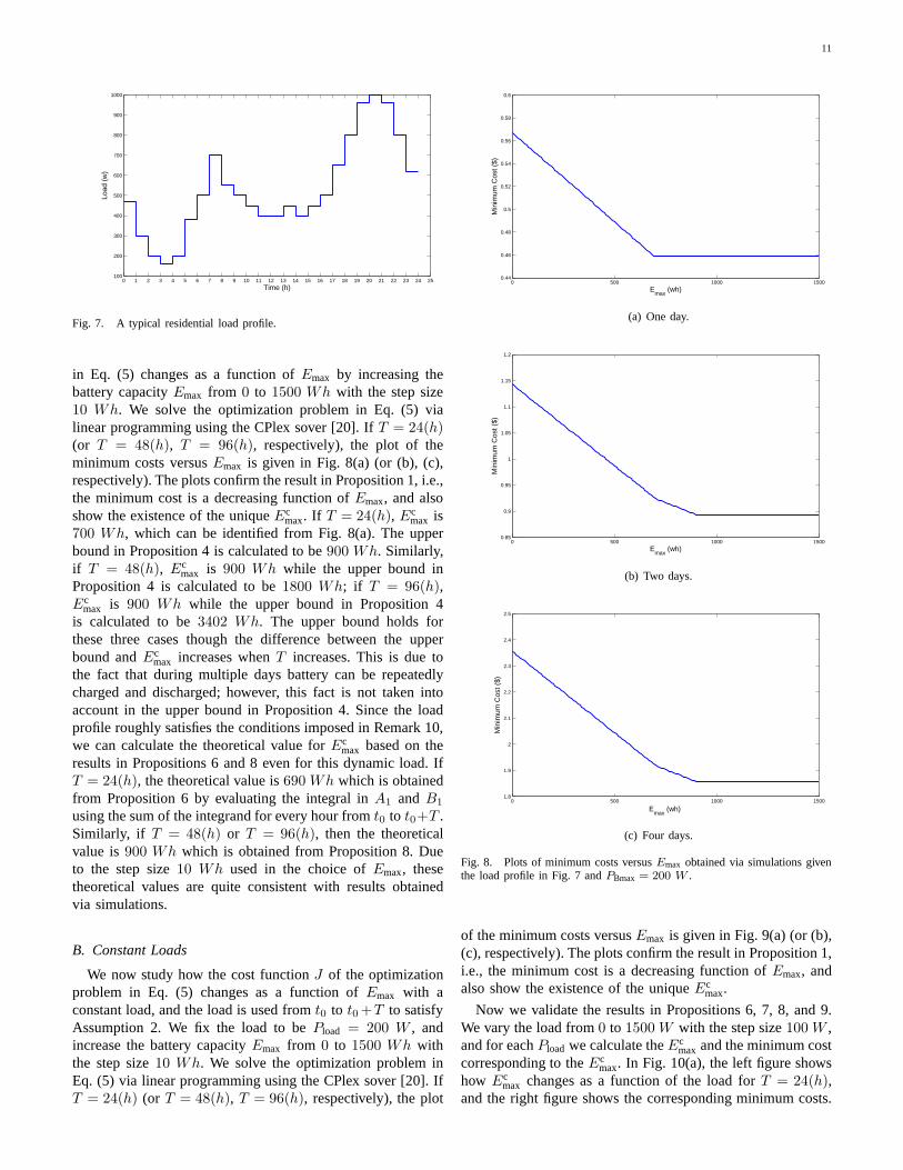
We first examine the upper bound in Proposition 4 usingdynamic loads. The load profile for one day is given in Fig. 7,which resembles the residential load profile in4 Fig. 8(b)in [15]. Note that one load peak appears in the early morning,and the other in the evening. For multiple day simulations,the load is periodic based on the load profile in Fig. 7. Westudy how the cost functionJ of the optimization problem

4However, simulations in [15] start at7AM so Fig. 7 is a shifted versionof the load profile in Fig. 8(b) in [15].

11

0 1 2 3 4 5 6 7 8 9 10 11 12 13 14 15 16 17 18 19 20 21 22 23 24 25100

200

300

400

500

600

700

800

900

1000

Time (h)

Load

(w

)

Fig. 7. A typical residential load profile.

in Eq. (5) changes as a function ofEmax by increasing thebattery capacityEmax from 0 to 1500 Wh with the step size10 Wh. We solve the optimization problem in Eq. (5) vialinear programming using the CPlex sover [20]. IfT = 24(h)(or T = 48(h), T = 96(h), respectively), the plot of theminimum costs versusEmax is given in Fig. 8(a) (or (b), (c),respectively). The plots confirm the result in Proposition 1, i.e.,the minimum cost is a decreasing function ofEmax, and alsoshow the existence of the uniqueEc

max. If T = 24(h), Ecmax is

700 Wh, which can be identified from Fig. 8(a). The upperbound in Proposition 4 is calculated to be900 Wh. Similarly,if T = 48(h), Ec

max is 900 Wh while the upper bound inProposition 4 is calculated to be1800 Wh; if T = 96(h),Ec

max is 900 Wh while the upper bound in Proposition 4is calculated to be3402 Wh. The upper bound holds forthese three cases though the difference between the upperbound andEc

max increases whenT increases. This is due tothe fact that during multiple days battery can be repeatedlycharged and discharged; however, this fact is not taken intoaccount in the upper bound in Proposition 4. Since the loadprofile roughly satisfies the conditions imposed in Remark 10,we can calculate the theoretical value forEc

max based on theresults in Propositions 6 and 8 even for this dynamic load. IfT = 24(h), the theoretical value is690 Wh which is obtainedfrom Proposition 6 by evaluating the integral inA1 andB1

using the sum of the integrand for every hour fromt0 to t0+T .Similarly, if T = 48(h) or T = 96(h), then the theoreticalvalue is900 Wh which is obtained from Proposition 8. Dueto the step size10 Wh used in the choice ofEmax, thesetheoretical values are quite consistent with results obtainedvia simulations.

B. Constant Loads

We now study how the cost functionJ of the optimizationproblem in Eq. (5) changes as a function ofEmax with aconstant load, and the load is used fromt0 to t0+T to satisfyAssumption 2. We fix the load to bePload = 200 W , andincrease the battery capacityEmax from 0 to 1500 Wh withthe step size10 Wh. We solve the optimization problem inEq. (5) via linear programming using the CPlex sover [20]. IfT = 24(h) (or T = 48(h), T = 96(h), respectively), the plot

0 500 1000 15000.44

0.46

0.48

0.5

0.52

0.54

0.56

0.58

0.6

Emax

(wh)

Min

imum

Cos

t ($)

(a) One day.

0 500 1000 15000.85

0.9

0.95

1

1.05

1.1

1.15

1.2

Emax

(wh)

Min

imum

Cos

t ($)

(b) Two days.

0 500 1000 15001.8

1.9

2

2.1

2.2

2.3

2.4

2.5

Emax

(wh)

Min

imum

Cos

t ($)

(c) Four days.

Fig. 8. Plots of minimum costs versusEmax obtained via simulations giventhe load profile in Fig. 7 andPBmax = 200 W .

of the minimum costs versusEmax is given in Fig. 9(a) (or (b),(c), respectively). The plots confirm the result in Proposition 1,i.e., the minimum cost is a decreasing function ofEmax, andalso show the existence of the uniqueEc

max.

Now we validate the results in Propositions 6, 7, 8, and 9.We vary the load from0 to 1500 W with the step size100 W ,and for eachPload we calculate theEc

max and the minimum costcorresponding to theEc

max. In Fig. 10(a), the left figure showshow Ec

max changes as a function of the load forT = 24(h),and the right figure shows the corresponding minimum costs.

12

0 500 1000 15000.09

0.1

0.11

0.12

0.13

0.14

0.15

0.16

0.17

0.18

Emax

(wh)

Min

imum

Cos

t ($)

(a) One day.

0 200 400 600 800 1000 1200 1400 16000.05

0.1

0.15

0.2

0.25

0.3

0.35

0.4

Emax

(wh)

Min

imum

Cos

t ($)

(b) Two days.

0 500 1000 15000.1

0.2

0.3

0.4

0.5

0.6

0.7

0.8

Emax

(wh)

Min

imum

Cos

t ($)

(c) Four days.

Fig. 9. Plots of minimum costs versusEmax obtained via simulations givenPload = 200 W andPBmax = 200 W .

The plot in the left figure is consistent with the result inProposition 7 except that the maximum ofEc

max is not unique.This is due to the fact that the load is chosen to be discretewith step size100 W . The right figure is consistent with theintuition that when the load is increasing, more electricityneeds to be purchased from the grid (resulting in a highercost). Note that the blue solid curve corresponds to the costswith Ec

max, while the red dotted curve corresponds toJmax, i.e.,the costs without battery. The plots forEc

max and the minimumcost forT = 48(h) andT = 96(h) are shown in Fig. 10(b)

0 500 1000 15000

100

200

300

400

500

600

700

Load (w)

Em

axc (

wh)

0 500 1000 15000

0.2

0.4

0.6

0.8

1

1.2

1.4

1.6

1.8

2

Load (w)

Cos

t ($)

Minimum costJ

max

(a) One day.

0 500 1000 15000

200

400

600

800

1000

1200

Load (w)

Em

axc (

wh)

0 500 1000 15000

0.5

1

1.5

2

2.5

3

3.5

4

Load (w)

Cos

t ($)

Minimum costJ

max

(b) Two days.

0 500 1000 15000

200

400

600

800

1000

1200

Load (w)

Em

axc (

wh)

0 500 1000 15000

1

2

3

4

5

6

7

8

Load (w)

Cos

t ($)

Minimum costJ

max

(c) Four days.

Fig. 10. Ecmax (left), and costs (bothJmax and the cost corresponding toEc

max,right) versus the fixed load obtained via simulations forPBmax=200 W .

and (c). The plots in the left figures of Fig. 10(b) and (c)are consistent with the result in Proposition 9. Note that asT

increases, the critical loadP cload decreases as shown in the left

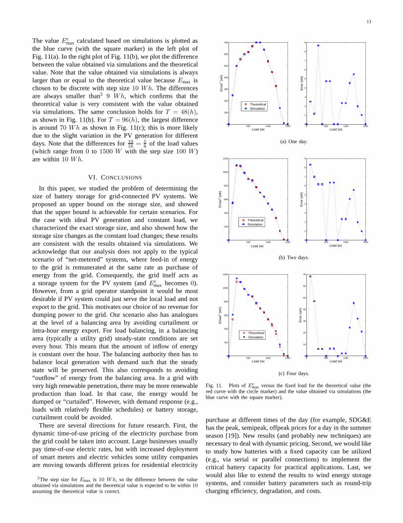
figures of Fig. 10.Now we examine the results in Proposition 6. ForT =

24(h), we evaluate the integral inA1 andB1 using the sumof the integrand for every hour fromt0 to t0 + T given afixed load, and then obtainEc

max; this value is denoted as thetheoretical value. The theoretical value is plotted as the redcurve (with the circle marker) in the left plot of Fig. 11(a).

13

The valueEcmax calculated based on simulations is plotted as

the blue curve (with the square marker) in the left plot ofFig. 11(a). In the right plot of Fig. 11(b), we plot the differencebetween the value obtained via simulations and the theoreticalvalue. Note that the value obtained via simulations is alwayslarger than or equal to the theoretical value becauseEmax ischosen to be discrete with step size10 Wh. The differencesare always smaller than5 9 Wh, which confirms that thetheoretical value is very consistent with the value obtainedvia simulations. The same conclusion holds forT = 48(h),as shown in Fig. 11(b). ForT = 96(h), the largest differenceis around70 Wh as shown in Fig. 11(c); this is more likelydue to the slight variation in the PV generation for differentdays. Note that the differences for1016 = 5

8 of the load values(which range from0 to 1500 W with the step size100 W )are within10 Wh.

VI. CONCLUSIONS

In this paper, we studied the problem of determining thesize of battery storage for grid-connected PV systems. Weproposed an upper bound on the storage size, and showedthat the upper bound is achievable for certain scenarios. Forthe case with ideal PV generation and constant load, wecharacterized the exact storage size, and also showed how thestorage size changes as the constant load changes; these resultsare consistent with the results obtained via simulations. Weacknowledge that our analysis does not apply to the typicalscenario of “net-metered” systems, where feed-in of energyto the grid is remunerated at the same rate as purchase ofenergy from the grid. Consequently, the grid itself acts asa storage system for the PV system (andEc

max becomes0).However, from a grid operator standpoint it would be mostdesirable if PV system could just serve the local load and notexport to the grid. This motivates our choice of no revenue fordumping power to the grid. Our scenario also has analoguesat the level of a balancing area by avoiding curtailment orintra-hour energy export. For load balancing, in a balancingarea (typically a utility grid) steady-state conditions are setevery hour. This means that the amount of inflow of energyis constant over the hour. The balancing authority then has tobalance local generation with demand such that the steadystate will be preserved. This also corresponds to avoiding“outflow” of energy from the balancing area. In a grid withvery high renewable penetration, there may be more renewableproduction than load. In that case, the energy would bedumped or “curtailed”. However, with demand response (e.g.,loads with relatively flexible schedules) or battery storage,curtailment could be avoided.

There are several directions for future research. First, thedynamic time-of-use pricing of the electricity purchase fromthe grid could be taken into account. Large businesses usuallypay time-of-use electric rates, but with increased deploymentof smart meters and electric vehicles some utility companiesare moving towards different prices for residential electricity

5The step size forEmax is 10 Wh, so the difference between the valueobtained via simulations and the theoretical value is expected to be within10assuming the theoretical value is correct.

0 500 1000 15000

100

200

300

400

500

600

700

Load (w)

Em

axc (

wh)

TheoreticalSimulation

0 500 1000 15000

1

2

3

4

5

6

7

8

9

Load (w)

Err

or (

wh)

(a) One day.

0 500 1000 15000

200

400

600

800

1000

1200

Load (w)

Em

axc (

wh)

TheoreticalSimulation

0 500 1000 15000

1

2

3

4

5

6

7

8

9

Load (w)

Err

or (

wh)

(b) Two days.

0 500 1000 15000

200

400

600

800

1000

1200

Load (w)

Em

axc (

wh)

TheoreticalSimulation

0 500 1000 15000

10

20

30

40

50

60

70

Load (w)

Err

or (

wh)

(c) Four days.

Fig. 11. Plots ofEcmax versus the fixed load for the theoretical value (the

red curve with the circle marker) and the value obtained via simulations (theblue curve with the square marker).

purchase at different times of the day (for example, SDG&Ehas the peak, semipeak, offpeak prices for a day in the summerseason [19]). New results (and probably new techniques) arenecessary to deal with dynamic pricing. Second, we would liketo study how batteries with a fixed capacity can be utilized(e.g., via serial or parallel connections) to implement thecritical battery capacity for practical applications. Last, wewould also like to extend the results to wind energy storagesystems, and consider battery parameters such as round-tripcharging efficiency, degradation, and costs.

14

REFERENCES

[1] H. Kanchev, D. Lu, F. COLAS, V. Lazarov, and B. Francois, “Energymanagement and operational planning of a microgrid with a PV-basedactive generator for smart grid applications,”IEEE Transactions onIndustrial Electronics, 2011.

[2] S. Teleke, M. E. Baran, S. Bhattacharya, and A. Q. Huang, “Rule-basedcontrol of battery energy storage for dispatching intermittent renewablesources,”IEEE Transactions on Sustainable Energy, vol. 1, pp. 117–124,2010.

[3] M. Lafoz, L. Garcia-Tabares, and M. Blanco, “Energy managementin solar photovoltaic plants based on ESS,” inPower Electronics andMotion Control Conference, Sep. 2008, pp. 2481–2486.

[4] W. A. Omran, M. Kazerani, and M. M. A. Salama, “Investigationof methods for reduction of power fluctuations generated from largegrid-connected photovoltaic systems,”IEEE Transactions on EnergyConversion, vol. 26, pp. 318–327, Mar. 2011.

[5] Y. Riffonneau, S. Bacha, F. Barruel, and S. Ploix, “Optimal powerflow management for grid connected PV systems with batteries,” IEEETransactions on Sustainable Energy, 2011.

[6] IEEE Recommended Practice for Sizing Lead-Acid Batteries for Stand-Alone Photovoltaic (PV) Systems, IEEE Std 1013-2007, IEEE, 2007.

[7] G. Shrestha and L. Goel, “A study on optimal sizing of stand-alone pho-tovoltaic stations,”IEEE Transactions on Energy Conversion, vol. 13,pp. 373–378, Dec. 1998.

[8] M. Akatsuka, R. Hara, H. Kita, T. Ito, Y. Ueda, and Y. Saito, “Esti-mation of battery capacity for suppression of a PV power plant outputfluctuation,” in IEEE Photovoltaic Specialists Conference (PVSC), Jun.2010, pp. 540–543.

[9] X. Wang, D. M. Vilathgamuwa, and S. Choi, “Determinationof batterystorage capacity in energy buffer for wind farm,”IEEE Transactions onEnergy Conversion, vol. 23, pp. 868–878, Sep. 2008.

[10] T. Brekken, A. Yokochi, A. von Jouanne, Z. Yen, H. Hapke,andD. Halamay, “Optimal energy storage sizing and control for wind powerapplications,”IEEE Transactions on Sustainable Energy, vol. 2, pp. 69–77, Jan. 2011.

[11] Q. Li, S. S. Choi, Y. Yuan, and D. L. Yao, “On the determination ofbattery energy storage capacity and short-term power dispatch of a windfarm,” IEEE Transactions on Sustainable Energy, vol. 2, pp. 148–158,Apr. 2011.

[12] B. Borowy and Z. Salameh, “Methodology for optimally sizing thecombination of a battery bank and pv array in a wind/PV hybridsystem,”IEEE Transactions on Energy Conversion, vol. 11, pp. 367–375, Jun.1996.

[13] R. Chedid and S. Rahman, “Unit sizing and control of hybrid wind-solarpower systems,”IEEE Transactions on Energy Conversion, vol. 12, pp.79–85, Mar. 1997.

[14] E. I. Vrettos and S. A. Papathanassiou, “Operating policy and optimalsizing of a high penetration res-bess system for small isolated grids,”IEEE Transactions on Energy Conversion, 2011.

[15] M. H. Rahman and S. Yamashiro, “Novel distributed powergeneratingsystem of PV-ECaSS using solar energy estimation,”IEEE Transactionson Energy Conversion, vol. 22, pp. 358–367, Jun. 2007.

[16] M. Ceraolo, “New dynamical models of lead-acid batteries,” IeeeTransactions On Power Systems, vol. 15, pp. 1184–1190, 2000.

[17] S. Barsali and M. Ceraolo, “Dynamical models of lead-acid batteries:Implementation issues,”IEEE Transactions On Energy Conversion,vol. 17, pp. 16–23, Mar. 2002.

[18] A. E. Bryson and Y.-C. Ho,Applied Optimal Control: Optimization,Estimation and Control. New York, USA: Taylor & Francis, 1975.

[19] SDG&E proposal to charge electric rates for different timesof the day: The devil lurks in the details. [Online]. Available:http://www.ucan.org/energy/electricity/sdgeproposalchargeelectric rates different times

[20] IBM ILOG CPLEX Optimizer. [Online]. Available:http://www-01.ibm.com/software/integration/optimization/cplex-optimizer