Two-Loop Controller for Maximizing Performance of aGrid-Connected Photovoltaic-Fuel Cell Hybrid Power Plant

Kyoungsoo Ro

Dissertation submitted to the Faculty of the Virginia Polytechnic Institute and State University in partial fulfillment of the requirements for the degree of

Doctor of Philosophy in Electrical Engineering

Saifur Rahman, Chairperson Hugh F. VanLandingham Robert P. Broadwater Yilu Liu John W. Roach

April 14, 1997 Blacksburg, Virginia

Keywords: Photovoltaics, Fuel Cells, Batteries, Neural Networks,Maximum Power Point Tracking Controller, Real andReactive Power Control, Environmental Evaluation.

ii

Two-Loop Controller for Maximizing Performance of aGrid-Connected Photovoltaic-Fuel Cell Hybrid Power Plant

Kyoungsoo Ro

(ABSTRACT)

The study started with the requirement that a photovoltaic (PV) power source should beintegrated with other supplementary power sources whether it operates in a stand-alone or grid-connected mode. First, fuel cells for a backup of varying PV power were compared in detailwith batteries and were found to have more operational benefits. Next, maximizing performanceof a grid-connected PV-fuel cell hybrid system by use of a two-loop controller was discussed.One loop is a neural network controller for maximum power point tracking, which extractsmaximum available solar power from PV arrays under varying conditions of insolation,temperature, and system load. A real/reactive power controller (RRPC) is the other loop. TheRRPC meets the system’s requirement for real and reactive powers by controlling incoming fuelto fuel cell stacks as well as switching control signals to a power conditioning subsystem. TheRRPC is able to achieve more versatile control of real/reactive powers than the conventionalpower sources since the hybrid power plant does not contain any rotating mass. Results of time-domain simulations prove not only effectiveness of the proposed computer models of the two-loop controller, but also their applicability for use in transient stability analysis of the hybridpower plant. Finally, environmental evaluation of the proposed hybrid plant was made in termsof plant’s land requirement and lifetime CO2 emissions, and then compared with that of theconventional fossil-fuel power generating forms.

iii

ACKNOWLEDGEMENTS

First of all, I would like to express my sincere gratitude to my advisor, Dr. SaifurRahman. His kind guidance, thorough comments and constant support have made it possible forme to make my dissertation complete. His teaching of the course “Alternate Energy Systems”had a great influence on my idea for this dissertation. I would also like to thank Dr. Hugh F.VanLandingham, Dr. Robert P. Broadwater, Dr. Yilu Liu and Dr. John W. Roach for their timeand advice as my advisory committee.

During my Ph.D. program, I have been associated with my colleagues at the Center forEnergy and the Global Environment. I would like to list here some of them to memorize andthank them: Yonael Teklu, Jiuping Pan, Majid Roghanizad, Concha Callwood, Irislav Drezga,Arnie de Castro, Joseph Wolete and Murat Dilek. I would like to specially thank Mr. Teklu forhis support to capture solar data from the photovoltaic test facility located on the roof ofWhittemore Hall in the Virginia Tech campus.

I would like to show my great appreciation to my wonderful parents, brothers and sisterfor their encouragement and support until I obtain a doctorate degree. I want to dedicate thisdissertation to my wife, Jeannie, and my daughter, Erin. My daughter was born just early thisyear on February 5, 1997 and she is very special to me because I have waited for her for sevenyears. It is my mother-in-law that I must thank for her hard and lovely labor for feeding mydaughter at night.

iv

TABLE OF CONTENTS

pageLIST OF FIGURES ------------------------------------------------------------------------------ vii

LIST OF TABLES ------------------------------------------------------------------------------- xi

CHAPTER 1. INTRODUCTION ------------------------------------------------------------- 11.1 Purpose ------------------------------------------------------------------------------------- 11.2 Problem Statement ------------------------------------------------------------------------ 3

CHAPTER 2. LITERATURE REVIEW ---------------------------------------------------- 62.1 Photovoltaic (PV) Systems --------------------------------------------------------------- 6 2.1.1 Background Information ---------------------------------------------------------- 6 2.1.2 State of The Art in PV Power Generation -------------------------------------- 92.2 Batteries ------------------------------------------------------------------------------------ 11 2.2.1 Introduction (Lead-Acid Battery) ----------------------------------------------- 11 2.2.2 Nickel-Cadmium Battery --------------------------------------------------------- 12 2.2.3 Sodium-Sulfur Battery ------------------------------------------------------------ 14 2.2.4 Zinc-Bromine Battery ------------------------------------------------------------- 15 2.2.5 Battery Applications to Power Systems ----------------------------------------- 152.3 Fuel Cells ----------------------------------------------------------------------------------- 17 2.3.1 Fuel Cell Background ------------------------------------------------------------- 17 2.3.2 Phosphoric Acid Fuel Cell (PAFC) ---------------------------------------------- 20 2.3.3 Molten Carbonate Fuel Cell (MCFC) ------------------------------------------- 22 2.3.4 Solid Oxide Fuel Cell (SOFC) --------------------------------------------------- 23 2.3.5 Fuel Cell Power Systems --------------------------------------------------------- 242.4 Neural Networks (NNs) ------------------------------------------------------------------ 25 2.4.1 Neural Network Background ---------------------------------------------------- 25 2.4.2 NN Applications to Power Systems --------------------------------------------- 272.5 Power Conditioning Subsystems (PCUs) ----------------------------------------------- 29 2.5.1 Background Information ---------------------------------------------------------- 29 2.5.2 PCU Applications to Renewable Power Sources ------------------------------ 32

CHAPTER 3. BATTERIES OR FUEL CELLS FOR PV POWER BACKUP ------- 343.1 Common Attributes ----------------------------------------------------------------------- 34

v

3.2 Different Attributes ----------------------------------------------------------------------- 36 3.2.1 Efficiency --------------------------------------------------------------------------- 36 3.2.2 Capacity Variation ----------------------------------------------------------------- 36 3.2.3 Flexibility in Operation ----------------------------------------------------------- 38 3.2.4 Cost --------------------------------------------------------------------------------- 42 3.2.5 Environmental Externality ------------------------------------------------------- 423.3 Summary ----------------------------------------------------------------------------------- 43

CHAPTER 4. DESCRIPTION OF PV-FUEL CELL HYBRID SYSTEM ----------- 454.1 Overall View of the PV-Fuel Cell Power Plant --------------------------------------- 454.2 Detailed Description of the Grid-Connected Hybrid System ------------------------ 46

CHAPTER 5. NEURAL NETWORK CONTROLLER FOR MPPT ----------------- 505.1 Neural Network (NN) Controller of the PV Power Plant ---------------------------- 505.2 Computer Model of the MPPT Control System --------------------------------------- 53

CHAPTER 6. REAL/REACTIVE POWER CONTROLLER (RRPC) --------------- 566.1 Real/Reactive Power Controller of the PV-Fuel Cell Hybrid System -------------- 566.2 Computer Model of the RRPC System ------------------------------------------------- 58

CHAPTER 7. CASE STUDIES --------------------------------------------------------------- 617.1 Sudden Decrease of Insolation with Constant Cell Temperature -------------------- 627.2 Slow Decrease of Insolation with Constant Cell Temperature ---------------------- 687.3 Sudden Increase of Insolation with Constant Cell Temperature --------------------- 747.4 Slow Increase of Insolation with Constant Cell Temperature ----------------------- 807.5 Variable Insolation and Cell Temperature --------------------------------------------- 867.6 Change of Power Commands with Variable Insolation and Cell Temperature ---- 91

CHAPTER 8. ENVIRONMENTAL EVALUATION ------------------------------------- 978.1 Introduction -------------------------------------------------------------------------------- 978.2 Land Requirement ------------------------------------------------------------------------ 978.3 CO2 Emissions ----------------------------------------------------------------------------- 998.4 Evaluation of the PV-Fuel Cell Hybrid Plant ------------------------------------------ 100

CHAPTER 9. CONCLUSIONS AND RECOMMENDATIONS ----------------------- 102

NOMENCLATURE ----------------------------------------------------------------------------- 105

REFERENCES ----------------------------------------------------------------------------------- 107

APPENDIX A. CO2 EMISSIONS FROM CONVENTIONAL FOSSIL FUEL POWER PLANTS ------------------------------------------------------------ 116

vi

APPENDIX B. CO2 EMISSIONS FROM PV POWER PLANTS ---------------------- 119

APPENDIX C. CO2 EMISSIONS FROM FUEL CELL POWER PLANTS --------- 121

VITA ------------------------------------------------------------------------------------------------ 122

vii

LIST OF FIGURES

pageFigure 1.1 Samples of PV power output variations ------------------------------------------- 2Figure 2.1 I-V characteristics of solar cells. (a) Influence of solar insolation.

(b) Influence of cell temperature --------------------------------------------------- 7Figure 2.2 Equivalent circuit for a solar cell -------------------------------------------------- 8Figure 2.3 Equivalent circuit for a battery ----------------------------------------------------- 13Figure 2.4 Typical plot of cell voltage vs. current density for a fuel cell ------------------ 18Figure 2.5 Equivalent circuit for a fuel cell ---------------------------------------------------- 19Figure 2.6 A typical neural network ------------------------------------------------------------ 25Figure 2.7 (a) A variable-frequency full bridge inverter. (b) Waveforms of the

ac voltage and current ---------------------------------------------------------------- 31Figure 3.1 Comparison of energy conversion processes ------------------------------------- 37Figure 3.2 Voltage characteristics of a battery at various discharge rates ----------------- 38Figure 3.3 Equally high efficiency of fuel cells at partial and full loads ------------------- 39Figure 3.4 Energy densities for fuel cells and batteries -------------------------------------- 40Figure 3.5 PV power variations requiring different battery capacities --------------------- 41Figure 4.1 Simplified overall diagram of the PV-fuel cell hybrid system ----------------- 46Figure 4.2 Diagram of the grid-connected PV system --------------------------------------- 47Figure 4.3 Diagram of the grid-connected fuel cell system --------------------------------- 48Figure 5.1 Neural network controller for MPPT in the PV array --------------------------- 51Figure 5.2 Computer model of the PV and MPPT control system -------------------------- 53Figure 6.1 Voltage notations for the PV-fuel cell hybrid system --------------------------- 57Figure 6.2 Real/reactive power control system of the fuel cell power plant --------------- 58Figure 6.3 Computer model of the fuel cell plant and RRPC system ----------------------- 59Figure 7.1 Sudden decrease of insolation from 100 mW/cm2 to 30 mW/cm2 -------------- 62Figure 7.2 (a) Transient response of the PV array voltage (Vpv) for sudden insolation

decrease from 100mW/cm2 to 30mW/cm2 --------------------------------------------- 63Figure 7.2 (b) Transient response of the PV array current (Ipv) for sudden insolation

decrease from 100mW/cm2 to 30mW/cm2 --------------------------------------------- 64Figure 7.2 (c) Transient response of the PV array DC power (Ppv) for sudden insolation

decrease from 100mW/cm2 to 30mW/cm2 --------------------------------------------- 64Figure 7.2 (d) Transient response of the PV array power (Pac1, Qac1) supplied to the grid

for sudden insolation decrease from 100mW/cm2 to 30mW/cm2 ------------------- 65Figure 7.2 (e) Transient response of the fuel cell voltage (Vfc) for sudden insolation

viii

decrease from 100mW/cm2 to 30mW/cm2 --------------------------------------------- 65Figure 7.2 (f) Transient response of the fuel cell current (Ifc) for sudden insolation

decrease from 100mW/cm2 to 30mW/cm2 --------------------------------------------- 66Figure 7.2 (g) Transient response of the fuel cell DC power (Pfc) for sudden insolation

decrease from 100mW/cm2 to 30mW/cm2 --------------------------------------------- 66Figure 7.2 (h) Transient response of the fuel cell power (Pac2, Qac2) supplied to the grid

for sudden insolation decrease from 100mW/cm2 to 30mW/cm2 ------------------- 67Figure 7.2 (i) Transient response of the total power (Pac, Qac) supplied to the grid

for sudden insolation decrease from 100mW/cm2 to 30mW/cm2 ------------------- 67Figure 7.3 Slow decrease of insolation from 100 mW/cm2 to 30 mW/cm2 ---------------- 68Figure 7.4 (a) Transient response of the PV array voltage (Vpv) for slow insolation

decrease from 100mW/cm2 to 30mW/cm2 --------------------------------------------- 69Figure 7.4 (b) Transient response of the PV array current (Ipv) for slow insolation

decrease from 100mW/cm2 to 30mW/cm2 --------------------------------------------- 70Figure 7.4 (c) Transient response of the PV array DC power (Ppv) for slow insolation

decrease from 100mW/cm2 to 30mW/cm2 --------------------------------------------- 70Figure 7.4 (d) Transient response of the PV array power (Pac1, Qac1) supplied to the grid

for slow insolation decrease from 100mW/cm2 to 30mW/cm2 ---------------------- 71Figure 7.4 (e) Transient response of the fuel cell voltage (Vfc) for slow insolation

decrease from 100mW/cm2 to 30mW/cm2 --------------------------------------------- 71Figure 7.4 (f) Transient response of the fuel cell current (Ifc) for slow insolation

decrease from 100mW/cm2 to 30mW/cm2 --------------------------------------------- 72Figure 7.4 (g) Transient response of the fuel cell DC power (Pfc) for slow insolation

decrease from 100mW/cm2 to 30mW/cm2 --------------------------------------------- 72Figure 7.4 (h) Transient response of the fuel cell power (Pac2, Qac2) supplied to the grid

for slow insolation decrease from 100mW/cm2 to 30mW/cm2 ---------------------- 73Figure 7.4 (i) Transient response of the total power (Pac, Qac) supplied to the grid

for slow insolation decrease from 100mW/cm2 to 30mW/cm2 ---------------------- 73Figure 7.5 Sudden increase of insolation from 30 mW/cm2 to 100 mW/cm2 -------------- 74Figure 7.6 (a) Transient response of the PV array voltage (Vpv) for sudden insolation

increase from 30mW/cm2 to 100mW/cm2 --------------------------------------------- 75Figure 7.6 (b) Transient response of the PV array current (Ipv) for sudden insolation

increase from 30mW/cm2 to 100mW/cm2 --------------------------------------------- 76Figure 7.6 (c) Transient response of the PV array DC power (Ppv) for sudden insolation

increase from 30mW/cm2 to 100mW/cm2 --------------------------------------------- 76Figure 7.6 (d) Transient response of the PV array power (Pac1, Qac1) supplied to the grid

for sudden insolation increase from 30mW/cm2 to 100mW/cm2 -------------------- 77Figure 7.6 (e) Transient response of the fuel cell voltage (Vfc) for sudden insolation

increase from 30mW/cm2 to 100mW/cm2 --------------------------------------------- 77Figure 7.6 (f) Transient response of the fuel cell current (Ifc) for sudden insolation

increase from 30mW/cm2 to 100mW/cm2 --------------------------------------------- 78Figure 7.6 (g) Transient response of the fuel cell DC power (Pfc) for sudden insolation

increase from 30mW/cm2 to 100mW/cm2 --------------------------------------------- 78

ix

Figure 7.6 (h) Transient response of the fuel cell power (Pac2, Qac2) supplied to the grid for sudden insolation increase from 30mW/cm2 to 100mW/cm2 -------------------- 79

Figure 7.6 (i) Transient response of the total power (Pac, Qac) supplied to the grid for sudden insolation increase from 30mW/cm2 to 100mW/cm2 ------------------------ 79

Figure 7.7 Slow increase of insolation from 30 mW/cm2 to 100 mW/cm2 ----------------- 80Figure 7.8 (a) Transient response of the PV array voltage (Vpv) for slow insolation

increase from 30mW/cm2 to 100mW/cm2 --------------------------------------------- 81Figure 7.8 (b) Transient response of the PV array current (Ipv) for slow insolation

increase from 30mW/cm2 to 100mW/cm2 --------------------------------------------- 82Figure 7.8 (c) Transient response of the PV array DC power (Ppv) for slow insolation

increase from 30mW/cm2 to 100mW/cm2 --------------------------------------------- 82Figure 7.8 (d) Transient response of the PV array power (Pac1, Qac1) supplied to the grid

for slow insolation increase from 30mW/cm2 to 100mW/cm2 ---------------------- 83Figure 7.8 (e) Transient response of the fuel cell voltage (Vfc) for slow insolation

increase from 30mW/cm2 to 100mW/cm2 --------------------------------------------- 83Figure 7.8 (f) Transient response of the fuel cell current (Ifc) for slow insolation

increase from 30mW/cm2 to 100mW/cm2 --------------------------------------------- 84Figure 7.8 (g) Transient response of the fuel cell DC power (Pfc) for slow insolation

increase from 30mW/cm2 to 100mW/cm2 --------------------------------------------- 84Figure 7.8 (h) Transient response of the fuel cell power (Pac2, Qac2) supplied to the grid

for slow insolation increase from 30mW/cm2 to 100mW/cm2 ---------------------- 85Figure 7.8 (i) Transient response of the total power (Pac, Qac) supplied to the grid

for slow insolation increase from 30mW/cm2 to 100mW/cm2 ---------------------- 85Figure 7.9 Variations of insolation and cell temperature ------------------------------------- 86Figure 7.10 (a) Transient response of the PV array voltage (Vpv) for real-time

variations of insolation and cell temperature ------------------------------------------ 87Figure 7.10 (b) Transient response of the PV array current (Ipv) for real-time

variations of insolation and cell temperature ------------------------------------------ 87Figure 7.10 (c) Transient response of the PV array DC power (Ppv) for real-time

variations of insolation and cell temperature ------------------------------------------ 88Figure 7.10 (d) Transient response of the PV array power (Pac1,Qac1) supplied to the grid

for real-time variations of insolation and cell temperature -------------------------- 88Figure 7.10 (e) Transient response of the fuel cell voltage (Vfc) for real-time

variations of insolation and cell temperature ------------------------------------------ 89Figure 7.10 (f) Transient response of the fuel cell current (Ifc) for real-time

variations of insolation and cell temperature ------------------------------------------ 89Figure 7.10 (g) Transient response of the fuel cell DC power (Pfc) for real-time

variations of insolation and cell temperature ------------------------------------------ 90Figure 7.10 (h) Transient response of the fuel cell power (Pac2, Qac2) supplied to the grid

for real-time variations of insolation and cell temperature -------------------------- 90Figure 7.10 (i) Transient response of the total power (Pac, Qac) supplied to the grid

for real-time variations of insolation and cell temperature -------------------------- 91Figure 7.11 (a) Transient response of the PV array voltage (Vpv) for change of power

x

commands with variable insolation and cell temperature ---------------------------- 92Figure 7.11 (b) Transient response of the PV array current (Ipv) for change of power

commands with variable insolation and cell temperature ---------------------------- 92Figure 7.11 (c) Transient response of the PV array power (Ppv) for change of power

commands with variable insolation and cell temperature ---------------------------- 93Figure 7.11 (d) Transient response of the PV array power (Pac1, Qac1) supplied to the grid

for change of power commands with variable insolation and cell temperature --- 93Figure 7.11 (e) Transient response of the fuel cell voltage (Vfc) for change of power

commands with variable insolation and cell temperature ---------------------------- 94Figure 7.11 (f) Transient response of the fuel cell current (Ifc) for change of power

commands with variable insolation and cell temperature ---------------------------- 94Figure 7.11 (g) Transient response of the fuel cell DC power (Pfc) for change of

power commands with variable insolation and cell temperature -------------------- 95Figure 7.11 (h) Transient response of the fuel cell power (Pac2, Qac2) supplied to the grid

for change of power commands with variable insolation and cell temperature --- 95Figure 7.11 (i) Transient response of the total power (Pac, Qac) supplied to the grid for

change of power commands with variable insolation and cell temperature ------- 96Figure 8.1 Land requirement and lifetime CO2 emissions for electric power plants -------101

xi

LIST OF TABLES

pageTable 2.1 Comparison of three types of fuel cells --------------------------------------------- 21Table 2.2 Key attributes of the principal learning procedures ------------------------------- 27Table 3.1 Capacity variations of a battery at various discharge rates ----------------------- 39Table 4.1 Power specifications of the single M55 PV module ------------------------------ 48Table 4.2 Specifications of the single 260-kW PAFC stack --------------------------------- 49Table 8.1 Land requirement for electric power plants ---------------------------------------- 98Table 8.2 CO2 emissions for electric power plants with a 30-year lifetime ---------------- 99Table A.1 CO2 productions from fossil fuel power plants with fuel treatment ------------ 118Table B.1 Accumulated energy requirements for PV power plants ------------------------- 119Table B.2 CO2 emissions of PV power plants ------------------------------------------------- 120

1

CHAPTER 1

INTRODUCTION

1.1 Purpose

As conventional fossil-fuel energy sources diminish and the world’s environmentalconcern about acid deposition and global warming increases, renewable energy sources (solar,wind, tidal, and geothermal, etc.) are attracting more attention as alternative energy sources.Among the renewable energy sources solar photovoltaic (PV) energy has been widely utilized insmall-size applications. It is also the most promising candidate for research and development forlarge-scale uses as the fabrication of less-costly photovoltaic devices becomes a reality.

PV power generation, which directly converts solar radiation into electricity, contains alot of significant advantages such as inexhaustible and pollution-free, silent and with no rotatingparts, and size-independent electricity conversion efficiency. Positive environmental effect ofphotovoltaics is replacing electricity generated in more polluting way or providing electricitywhere none was available before. With increasing penetration of solar photovoltaic devices,various anti-pollution apparatuses can be operated by solar PV power; for example, waterpurification by electrochemical processing or stopping desert expansion by photovoltaic waterpumping with tree implantation [17].

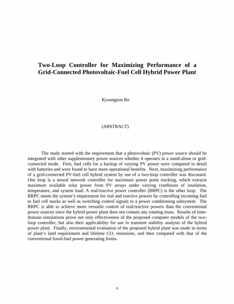
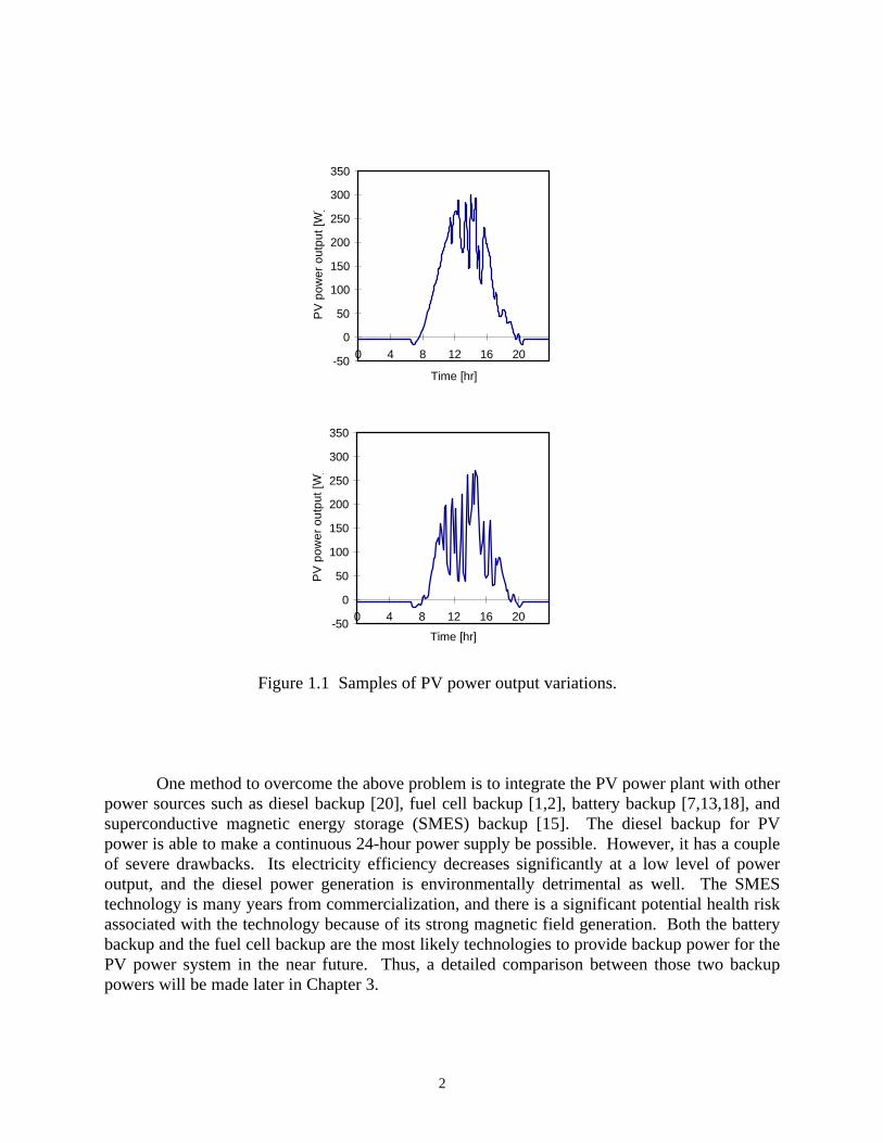
From an operational point of view, a photovoltaic array experiences large variations ofits output power under intermittent weather conditions. Those phenomena may causeoperational problems at a central control center in a power utility, such as excessive frequencydeviations, spinning reserve increase, etc. Figure 1.1 illustrates two samples of PV powervariations for one day. The data was measured at a time interval of 10 minutes from the PV testfacility in the Virginia Tech campus on July 10 and July 18, 1993. When photovoltaic powerpenetration approaches about 10% of the system load, it is difficult for the conventional powergeneration system to keep track of the rapid PV power output changes [10].

2

-50

0

50

100

150

200

250

300

350

0 4 8 12 16 20

Time [hr]

PV

pow

er o

utpu

t [W

]

-50

0

50

100

150

200

250

300

350

0 4 8 12 16 20

Time [hr]

PV

pow

er o

utpu

t [W

]

Figure 1.1 Samples of PV power output variations.

One method to overcome the above problem is to integrate the PV power plant with otherpower sources such as diesel backup [20], fuel cell backup [1,2], battery backup [7,13,18], andsuperconductive magnetic energy storage (SMES) backup [15]. The diesel backup for PVpower is able to make a continuous 24-hour power supply be possible. However, it has a coupleof severe drawbacks. Its electricity efficiency decreases significantly at a low level of poweroutput, and the diesel power generation is environmentally detrimental as well. The SMEStechnology is many years from commercialization, and there is a significant potential health riskassociated with the technology because of its strong magnetic field generation. Both the batterybackup and the fuel cell backup are the most likely technologies to provide backup power for thePV power system in the near future. Thus, a detailed comparison between those two backuppowers will be made later in Chapter 3.

3

A fuel cell power is a very attractive option being used with an intermittent powergeneration source like the PV power because the fuel cell power system contains lots of greatfeatures such as high efficiency, fast load-response, modular production and fuel flexibility. Itsfeasibility in coordination with a photovoltaic power system has been successfully demonstratedfor both grid-connected and stand-alone applications [1]. Due to the fast ramping capability ofthe fuel cell power system, a PV-fuel cell hybrid system may be able to solve the PV’s inherentproblem of intermittent power generation. Unlike a storage battery, which also containsattractive attributes such as fast response rate, modular construction and flexibility for siteselection, the fuel cell power can produce electricity continuously to support the PV power.Therefore, the quality of overall power generated from the PV-fuel cell hybrid power plant maybe improved. The combination of the photovoltaic and fuel cell power plants is now a viabletechnology to commercial applications.

Environmental impacts of the fuel cell power generation are relatively small in contrastto other fossil-fuel power sources. Since chemical reactions inside the fuel cell stack areaccomplished by catalysts, it must require a low sulfur-content fuel. Since the fuel cell stackoperates electrochemically at lower temperature than other thermomechanical power plants, itgenerates very little amount of NOx. NOx forms mainly from nitrogen contained in thecombustion air if fuels used have low nitrogen content. Low-emission characteristics of the fuelcell power plant may allow some utilities to offset the costs of installing additional emissioncontrol equipment. Moreover, their high efficiency is able to result in lower fossil-fuel CO2

emissions, which will help reduce the rate of global warming. Therefore, the fuel cell powersystem has a great potential for being coordinated with the PV array to smooth out the PVpower’s fluctuations.

One purpose of this study is to prove that the fuel cell power has the best potential for thePV power backup. Designing an efficient controller for a PV-fuel cell hybrid power plant isanother purpose. The controller consists of two loops; one loop is a neural network controllerfor MPPT (Maximum Power Point Tracking) and the other is a real/reactive power controller.The two-loop controller is able not only to achieve maximum utilization of the available solarpower but also to satisfy the hybrid power plant’s operational requirement for real and reactivepower control. Thus, such a hybrid power plant can be used as a reliable power generationsource either on a stand-alone or a grid-interactive mode. The other purpose is to establishsimplified computer models of the two-loop controller. Those computer models might be usefulfor use in transient stability analysis of a power system that includes the PV-fuel cell hybridsystem.

1.2 Problem Statement

4

It has been well-proven that a photovoltaic power source should be integrated with otherpower sources, whether used in either a stand-alone or grid-connected mode. This study startswith a comparison between batteries and fuel cells for PV power backup since these two powersources are the most likely technologies for PV power supplement. Then it will be proven thatfuel cells have more benefits when they are applied to support a PV power varying severely oninclement weather days.

A technique for maximizing performance of a grid-connected PV-fuel cell hybrid powerplant by using a two-loop controller is discussed. One loop is the neural network controller formaximum power point tracking (MPPT) in the PV array, which extracts maximum availablesolar power at varying weather conditions. A centralized PV power plant requires much largerinitial capital investment compared to other power generation sources. Thus, it is imperative toextract as much available solar energy as possible from the PV array; if not, the photovoltaicpower system might lose some of the valuable solar energy. Nonlinear current-voltage (I-V)characteristics of a PV module match well to a neural network application. In order that the PVarray keep track of its maximum power points, the outputs of the neural network controllershould generate optimal switching signals to the power conditioning subsystem (PCS) of the PVarray. The PCS usually consists of a full-bridge dc to ac inverter.

A real/reactive power controller (RRPC) installed at the fuel cell power plant is the otherloop. The RRPC is going to achieve the utility grid’s requirement for real and reactive powersby controlling the fuel cell stacks and the PCS. Real power control is made by regulating boththe incoming fuel (mostly natural gas) to the fuel cell stacks and the switching control signals tothe PCS of the fuel cell power plant. Reactive power is controlled only by generatingappropriate switching scheme to the PCS. Simplified computer models of the two-loopcontroller are developed. Time-domain simulations prove an applicability of the two-loopcontroller for use in a transient stability analysis of the hybrid power plant.

I continue to discuss an environmental evaluation of the proposed PV-fuel cell hybridpower plant compared with the conventional power generation forms. Two categories throughwhich the evaluation is accomplished are land area requirement for the hybrid power plantconstruction and its lifetime CO2 emissions. The CO2 emissions of the hybrid power plant arecaused by fuel consumption during its life-long period, and construction, operation andmaintenance (O&M) of the hybrid power plant.

The major contributions that are made in this dissertation are summarized below:

(i) Compare batteries with fuel cells for a backup of a PV power that fluctuates oninclement weather days, and verify that the fuel cells have more benefits for thatpurpose. It will be discussed in Chapter 3.

(ii) Apply a neural network controller to always extract maximum available solarpower from the PV array under changing conditions of solar insolation, cell

5

temperature and utility system load. Chapter 5 will describe the neural networkcontroller for the PV array.

(iii) Design a real/reactive power controller for the fuel cell power plant so that thePV-fuel cell hybrid system satisfies the utility system’s requirement for real andreactive powers. Real power control is achieved by effectively controlling boththe fuel injected to the fuel cell stacks and the switching scheme of the full-bridge dc-ac inverter. Reactive power is controlled by generating appropriateswitching signals to the inverter. Chapter 6 will give the method to design theRRPC.

(iv) Present simplified computer models of the neural network controller for MPPTand the RRPC system in the grid-connected PV-fuel cell hybrid power plant.Chapter 5 and 6 explain these computer models. Then Chapter 7 verifies theperformance of the computer models by time-domain computer simulations.

(v) Evaluate environmental impacts of the proposed PV-fuel cell hybrid system interms of land requirement for the plant construction and its lifetime CO2

emissions. They will be discussed in Chapter 8.

The other chapters will support to better-understand this dissertation. Chapter 2 covers a broadrange of background information on photovoltaics, batteries, fuel cells, neural networks andpower conditioning subsystems. Chapter 4 describes the PV-fuel cell hybrid power plant in theoverall view and detailed view. Conclusions and Recommendations will be given in Chapter 9,which is followed by Nomenclature and References. Appendix A gives calculations of CO2

emissions from conventional fossil fuel power plants. CO2 emissions from PV power plants andfuel cell power plants are computed in Appendix B and Appendix C, respectively.

6

CHAPTER 2

LITERATURE REVIEW

A comprehensive literature search has been made in the areas that would get together toconstitute the proposed PV-fuel cell hybrid power plant and control systems. This chapterconsists of five sections and discusses photovoltaic systems, batteries, fuel cells, neural networksand power conditioning subsystems in that order. The objective of this discussion is to make iteasy to understand this dissertation.

2.1 Photovoltaic (PV) Systems

2.1.1 Background Information

Figure 2.1 illustrates typical current-voltage (I-V) curves of an ARCO M55 solar cellmodule according to the variations of insolation level and cell temperature. The figure alsoincludes the loci of maximum power points and equivalent resistive load lines. Open-circuitvoltage of the solar cell module, a crosspoint of the curve to the vertical axis, varies little withinsolation changes. It is inversely proportional to temperature, or a rise in temperature producesa decrease in voltage. Short-circuit current, a crosspoint of the curve to the horizontal axis, isdirectly proportional to insolation and is relatively steady in changing temperature.

The solar cell module acts like a constant current source for most part of its I-V curve. Itcan provide a constant current from zero to around 15V despite a changing resistive load. As theresistance continues to increase, the curve reaches a breakdown point and starts to drop to zero.

As demonstrated in Figure 2.1, an increase in solar insolation causes the output current toincrease and the vertical part of the curve to move rightward. An increase in cell temperature

7

0

5

10

15

20

25

30

0.01 0.51 1.01 1.51 2.01 2.51 3.01 3.51 4.01

Current (A)

Vol

tage

(V

)

20 40

60 80 100 120

Resistive loadMaximum power points

(a) Influence of solar insolation [mW/cm2] (Temperature = 25o

C).

10

12

14

16

18

20

22

24

26

0.01 0.51 1.01 1.51 2.01 2.51 3.01 3.51

Current (A)

Vol

tage

(V

)

6545

255

-15

Maximum power points

Resistive load

(b) Influence of cell temperature [oC] (Insolation = 100 mW/cm2).

Figure 2.1 I-V characteristics of solar cells.

8

causes the voltage to drop, while decreasing temperature produces the opposite effect. Thus theI-V curves display how a solar cell responds to all possible loads under a certain set of insolationand cell temperature conditions.

An operating point of a solar cell will move by varying insolation, cell temperature, andload values. For a given insolation and operating temperature, the output power depends on thevalue of a load resistance. As the load increases (or the resistance decreases), the operating pointmoves along the curve forward the right. So only one load value makes the PV generatorproduce maximum power. A maximum power point trajectory, which is positioned at the kneeof the I-V curve, represents the nearly constant output voltage of the PV generator at varyingsolar insolation condition. When the temperature varies, the maximum power points aregenerated in such a manner that the output current stays approximately constant.

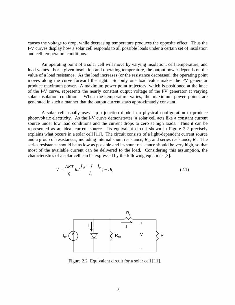
A solar cell usually uses a p-n junction diode in a physical configuration to producephotovoltaic electricity. As the I-V curve demonstrates, a solar cell acts like a constant currentsource under low load conditions and the current drops to zero at high loads. Thus it can berepresented as an ideal current source. Its equivalent circuit shown in Figure 2.2 preciselyexplains what occurs in a solar cell [11]. The circuit consists of a light-dependent current sourceand a group of resistances, including internal shunt resistance, Rsh, and series resistance, Rs. Theseries resistance should be as low as possible and its shunt resistance should be very high, so thatmost of the available current can be delivered to the load. Considering this assumption, thecharacteristics of a solar cell can be expressed by the following equations [3].

V AKTq

I I II

IRph o

os=

− +−ln( ) (2.1)

Iph

Ij

Rsh

Rs

RV

+

-

I

Figure 2.2 Equivalent circuit for a solar cell [11].

9

or

I I Iq V IR

AKTph os= −

+−[exp{

( )} ]1 (2.2)

where

I I K Tph scr i= + −[ ( )]298 100λ (2.3)

I ITT

qEBK T To or

r

G

r

= −( ) exp[ ( )]3 0 1 1 (2.4)

From the above equations, we can conclude that the output current and voltage of a PV moduleare affected by solar insolation and operating cell temperature.

The fill factor of a silicon solar cell is defined as the ratio of peak power to the powercomputed by multiplying the open-circuit voltage by the short-circuit current. That reflects howmuch series resistance and how little shunt resistance there is in the solar cell. A good fill factorranges from 0.6 to 0.8. As the solar cell degrades with age, its series resistance tends to increaseresulting in a lower fill factor.

2.1.2 State of The Art in PV Power Generation

As solar cell manufacturing technologies improve steadily, commercial applications ofPV power generation have increased from stand-alone to utility-connected generating systems.Interconnection and operation of a PV power unit are not same as electric utilities have beendoing for the conventional power plants. It requires specific PV interface, protection schemes,storage devices, and control mechanisms. Especially because the PV power output is directlyaffected by the changes of weather (solar intensity, temperature, etc.), it becomes considerablycomplicated to efficiently control the PV power plant.

Kalaitzakis and Vachtsevanos [7] proposed a methodology for the effective integration ofphotovoltaic devices into the electric utility distribution network operations. They focused onthe storage requirements for control and stability purposes, power flow control, and powermodulating device contributing to the improvement of system stability. System stability can beimproved by monitoring the variations in system frequency, utility grid bus voltage, and the realpower at the inverter output bus. Finally, their simulation studies indicate that an application ofthe proposed control approach may result in reduced load following requirements forconventional power generating units, and better power quality and stability of the interconnectedsystem.

10

Khallat and Rahman [49] presented the concept of adding fuel cells to provideoperational support to a PV system. They determined the capacity credit of the PV system whenthese are included in the utility generation mix. The study indicated that the capacity credit ofthe PV system continues to rise with increasing penetration up to 16.8% and then it decreases.By the comparison of the capacity credit available and the fuel cell requirements, their netdifference increases from 4.2% to 16.8% penetration. It was concluded that there is an upperlimit for PV penetration with fuel cell support for a power system.

Rahman and Kroposki [52] discussed a performance evaluation of crystalline andamorphous silicon PV modules in the light of their capability to operate as a demand sidemanagement (DSM) tool. The analysis of collected data showed a significant difference in thecell efficiency, which is 10% for the single crystalline cells and around 3% for the amorphouscells. The authors compared the plane-of-array insolations under different tilt conditions; thelargest gain in insolation due to 2-axis tracking over a semi-annual tilt change is 12.2% while thesmallest gain is 4.9%.

Hiyama et al. [21, 22] presented a neural network application to the identification of theoptimal operating point of PV modules and designed a PI-type controller for real-time maximumpower tracking. Optimal operating voltages are identified through the proposed neural networkby using the open-circuit voltages measured from monitoring cells and optimal operatingcurrents are calculated from the measured short-circuit currents. The output of the neuralnetwork goes through the PI controller to the voltage control loop of the inverter to change theterminal voltage of the PV system to the identified optimal one.

Ohnishi et al. [17] described applications of solar cells especially to residential areas suchas solar-powered air conditioners and grid-connected PV power generating systems. Concernedabout the disadvantages of solar cells, namely that they cannot generate power at night and theiroutput fluctuates dramatically depending on solar intensities, they proposed a Global EnergyNetwork Equipped with Solar cells and International Superconductor grids (GENESIS) forresolving these problems. They forecasted that in the year 2000 the world energy demand willbe the equivalent of 14 billion kilo-liter of crude oil per year. To meet that requirements,800km2 of solar cells would be needed, assuming a conversion efficiency of 10%. The studyconcluded that that plan is quite feasible because about 4% of the world’s desert area wouldsuffice for that purpose.

Schaefer and Hagedorn [16] compared PV power generation with the conventionalpower generation forms in terms of some environmental characteristics. Solar power is the mostsurface intensive power generation form due to its low efficiency and low energy density ofsolar radiation. They calculated the accumulated energy consumption in the fabrication of solarcells and the construction of PV power plants, and, for single-crystalline solar cells, those valuesare 11,000kWh/kWp and 12,200kWh/kWp, respectively. The accumulated energy consumptionin the solar cell fabrication and PV power plant construction involves CO2 emissions, which can

11

be estimated using emission factors within a given energy supply structure. In the case ofGermany, equivalent CO2 emissions of PV power plants for a lifetime of 20 years are 70gCO2/kWh for single-crystalline solar cells.

2.2 Batteries

2.2.1 Introduction (Lead-Acid Battery)

A storage battery is a chemical device reversible in its action, which stores chemicalenergy for use later as electrical energy. The chemical energy stored in electrodes of a batterycell is converted to electrical energy when the cell is discharging. Electrical energy is applied tothe battery during the operation of charging, so the electric current produces chemical changes inthe battery.

The most commonly used storage battery for utility applications is the lead-acid type.The fundamental parts of a lead-acid battery cell are two dissimilar electrodes immersed in anelectrolyte, namely

Anode(-) : Spongy lead (Pb)Cathode(+) : Lead dioxide (PbO2)Electrolyte : Dilute solution of sulfuric acid (H2SO4)

When a battery cell is connected to a circuit, it allows charge to flow around the circuit.In its external part, the charge flow is electrons resulting in electrical current. Within the cell,the charge flows in the form of ions that are transported from one electrode to the other. Thecathode, highly oxidized lead dioxide, receives electrons from the external circuit on discharge.These electrons react with the cathode material, which leaves some lead free to combine withsulphate ions to form lead sulphate. Hydrogen ions move in to the cathode and combine withoxygen to form water. At the anode, reactions between the anode material and the sulphate ionsresult in excessive electrons that can be donated to the external circuit. In this way the chemicalenergy stored in the battery is converted to electrical energy.

The chemical reaction occurred at the anode is

Pb + SO42- PbSO4 + 2e-

Discharge

Charge (2.5)

and that at the cathode is

12

PbO2 + SO42- + 4H+ + 2e- PbSO4 + 2H2O

Discharge

Charge (2.6)

Therefore, the net reaction can be expressed as follows

PbO2 + Pb + 2H2SO4 2PbSO4 + 2H2O

Discharge

Charge (2.7)

A battery system is a group of battery cells that supply dc power at a nominal voltage toan electrical load. The number of cells connected in series determines the nominal voltage of thebattery system, and the capacity of the battery system is the basic factor in determining thedischarge rate. The voltage is the force enforcing each of the electrons coming out of the batteryand the capacity is the number of electrons that can be obtained from the battery. While thevoltage is fixed by cell chemistry, the capacity is variable depending on the quantity of activematerials. The discharge rate of a battery is given in terms of ampere-hours (Ah) to a particulardischarge voltage level. For the lead-acid battery, its nominal cell voltage is 2V and the nominaldischarge voltage level is 1.75V/cell, or approximately 87.5% of the nominal cell voltage rating.

The equivalent circuit for a battery is shown in Figure 2.3. The internal resistance is dueto the resistance of electrolyte and electrode. Self-discharge resistance is a result of electrolysisof water at high voltages and slow leakage across the battery terminals at low voltages. Theovervoltage is modeled as an RC circuit with a time constant in the order of minutes [36, 37].

Lead-acid battery systems are a near-term solution to power regulation needs for electricutilities. However, the technology has suffered from a slow acceptance into power markets dueto such factors as uncertain return on investment and difficulty in quantifying benefits.Recently, there is worldwide interest to develop alternatives to lead-acid batteries that are able toproduce high performance at low cost. Advanced batteries such as nickel-cadmium, sodium-sulfur and zinc-bromine are likely to emerge in the next decade.

2.2.2 Nickel-Cadmium Battery

As the nickel-cadmium battery promoters claim its superiority over the lead-acidbatteries in spite of the high capital cost, there are several tries to adopt the nickel-cadmiumbatteries for use in PV applications. One major reason for that is its longer life and operationalreliability. It is undamaged by complete discharge and overcharge.

The active material of the cathode is nickel hydrate with graphite and that of the anode iscadmium sponge, with additives to aid conductivity. The electrolyte is a solution of potassium

13

Rov

Cov

Rbat

Cb RbVoc

+

-

V

+

-

Rov - overvoltage resistanceCov - overvoltage capacitanceRbat - internal resistanceRb - self-discharge resistanceCb - battery capacitanceVoc - open circuit voltageV - battery voltage

Figure 2.3 Equivalent circuit for a battery [36].

hydroxide (KOH), including a small amount of lithium hydroxide (LiOH) to improve capacity.The charge-discharge reaction may be written as

2Ni(OH)3 + Cd 2Ni(OH)2 + Cd(OH)2Discharge

Charge (2.8)

The nominal voltage of a nickel-cadmium battery on discharge is 1.2V. When thebattery is connected to an external load, its voltage falls to a value depending on discharge rateand state of charge. The normal final discharge voltage is 1.05V/cell. The battery ischaracterized by a low self-discharge rate; its capacity drops to about 80% in a year under opencircuit conditions. Its operating temperature range is between -50 to 60oC and the batterycapacity drops to half of the nominal capacity at -50oC.

Nickel-cadmium battery system contains its significant features for PV applications.With respect to charging conditions, the nickel-cadmium battery offers more than 80% chargingefficiency, as high as a lead-acid battery does. It does not suffer from complete discharge orovercharge in contrast to the lead-acid battery and its annual maintenance is less costly that thatof the lead-acid battery. At low temperatures there is a need for the lead-acid battery to be keptin a high state of charge to avoid freezing, which would make it less cost effective over thenickel-cadmium battery.

14

A disadvantage associated with the nickel-cadmium battery is its memory effect and highcapital cost. Repeated use in the same way causes the battery to adjust itself to a certain capacityin relation to its load. Its cost per ampere-hour of capacity is considered as another disadvantagefor wide use although the battery is promoted as an alternative to the lead-acid battery in PVapplications.

2.2.3 Sodium-Sulfur Battery

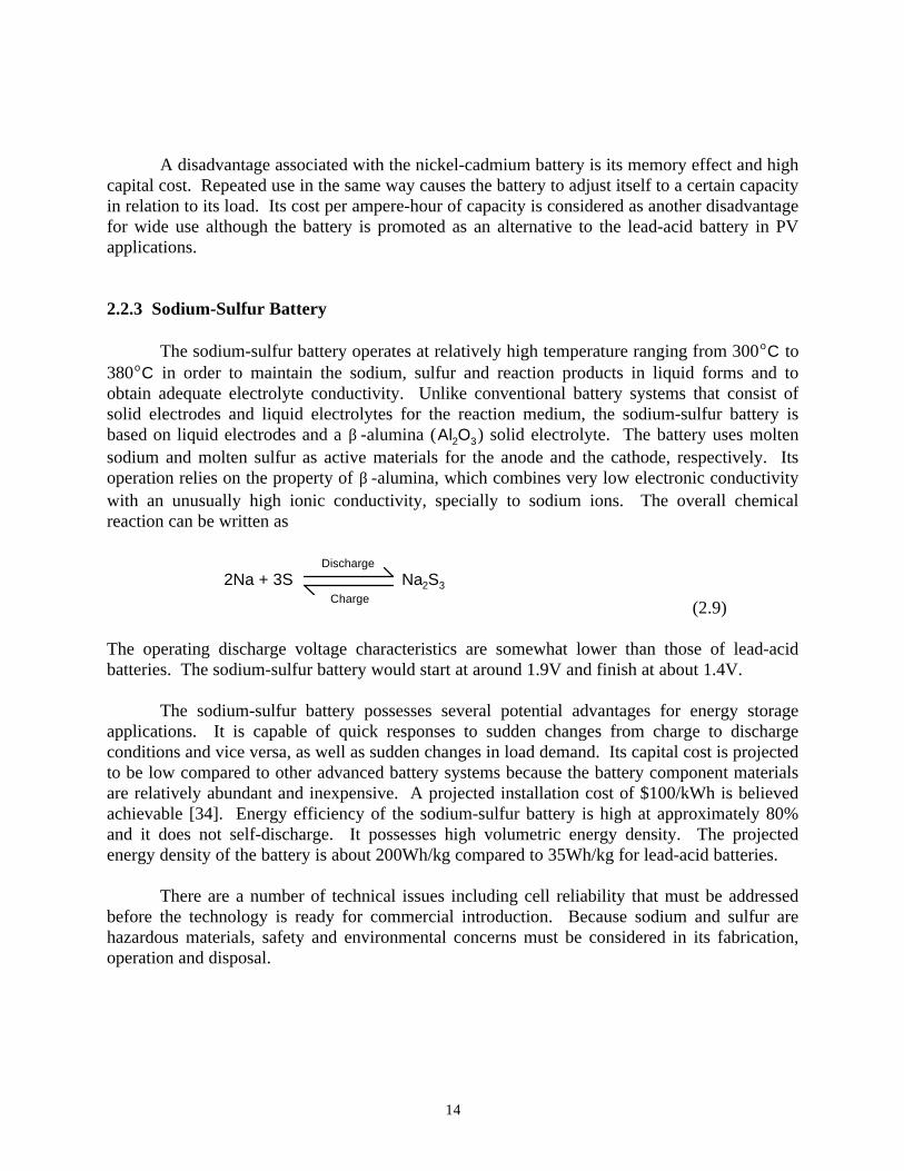
The sodium-sulfur battery operates at relatively high temperature ranging from 300oC to380oC in order to maintain the sodium, sulfur and reaction products in liquid forms and toobtain adequate electrolyte conductivity. Unlike conventional battery systems that consist ofsolid electrodes and liquid electrolytes for the reaction medium, the sodium-sulfur battery isbased on liquid electrodes and a β -alumina (Al O2 3) solid electrolyte. The battery uses moltensodium and molten sulfur as active materials for the anode and the cathode, respectively. Itsoperation relies on the property of β -alumina, which combines very low electronic conductivitywith an unusually high ionic conductivity, specially to sodium ions. The overall chemicalreaction can be written as

2Na + 3S Na2S3

Discharge

Charge (2.9)

The operating discharge voltage characteristics are somewhat lower than those of lead-acidbatteries. The sodium-sulfur battery would start at around 1.9V and finish at about 1.4V.

The sodium-sulfur battery possesses several potential advantages for energy storageapplications. It is capable of quick responses to sudden changes from charge to dischargeconditions and vice versa, as well as sudden changes in load demand. Its capital cost is projectedto be low compared to other advanced battery systems because the battery component materialsare relatively abundant and inexpensive. A projected installation cost of $100/kWh is believedachievable [34]. Energy efficiency of the sodium-sulfur battery is high at approximately 80%and it does not self-discharge. It possesses high volumetric energy density. The projectedenergy density of the battery is about 200Wh/kg compared to 35Wh/kg for lead-acid batteries.

There are a number of technical issues including cell reliability that must be addressedbefore the technology is ready for commercial introduction. Because sodium and sulfur arehazardous materials, safety and environmental concerns must be considered in its fabrication,operation and disposal.

15

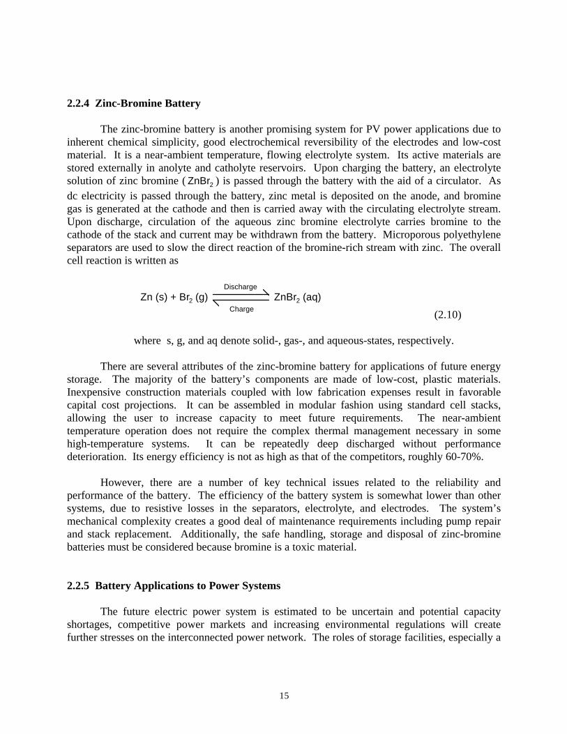
2.2.4 Zinc-Bromine Battery

The zinc-bromine battery is another promising system for PV power applications due toinherent chemical simplicity, good electrochemical reversibility of the electrodes and low-costmaterial. It is a near-ambient temperature, flowing electrolyte system. Its active materials arestored externally in anolyte and catholyte reservoirs. Upon charging the battery, an electrolytesolution of zinc bromine ( ZnBr2 ) is passed through the battery with the aid of a circulator. Asdc electricity is passed through the battery, zinc metal is deposited on the anode, and brominegas is generated at the cathode and then is carried away with the circulating electrolyte stream.Upon discharge, circulation of the aqueous zinc bromine electrolyte carries bromine to thecathode of the stack and current may be withdrawn from the battery. Microporous polyethyleneseparators are used to slow the direct reaction of the bromine-rich stream with zinc. The overallcell reaction is written as

Zn (s) + Br2 (g) ZnBr2 (aq)Discharge

Charge (2.10)

where s, g, and aq denote solid-, gas-, and aqueous-states, respectively.

There are several attributes of the zinc-bromine battery for applications of future energystorage. The majority of the battery’s components are made of low-cost, plastic materials.Inexpensive construction materials coupled with low fabrication expenses result in favorablecapital cost projections. It can be assembled in modular fashion using standard cell stacks,allowing the user to increase capacity to meet future requirements. The near-ambienttemperature operation does not require the complex thermal management necessary in somehigh-temperature systems. It can be repeatedly deep discharged without performancedeterioration. Its energy efficiency is not as high as that of the competitors, roughly 60-70%.

However, there are a number of key technical issues related to the reliability andperformance of the battery. The efficiency of the battery system is somewhat lower than othersystems, due to resistive losses in the separators, electrolyte, and electrodes. The system’smechanical complexity creates a good deal of maintenance requirements including pump repairand stack replacement. Additionally, the safe handling, storage and disposal of zinc-brominebatteries must be considered because bromine is a toxic material.

2.2.5 Battery Applications to Power Systems

The future electric power system is estimated to be uncertain and potential capacityshortages, competitive power markets and increasing environmental regulations will createfurther stresses on the interconnected power network. The roles of storage facilities, especially a

16

battery energy storage (BES) system as power regulation and energy management are beingrecognized as a practical solution to future operating uncertainty.

BES systems have been interesting power utilities as an option to supply power at peak-time to achieve load leveling. For example, Southern California Edison’s Chino battery planthas demonstrated the capability of lead-acid batteries to satisfy the utility’s operational andperformance requirements for load leveling. Recently, other dynamic benefits of BES have beenidentified, such as load following, spinning reserve, power factor correction, long linestabilization, and voltage and frequency regulation, etc. [34, 38]. The BES system is predictedto become an economically attractive option for utilities in the future due to those benefitscoupled with the ability to provide peak power.

Abraham et al. [32] presented the major types of batteries being developed for loadleveling and a generic description of the balance of plant (BOP). It is used to define thecomponents needed to integrate the battery facility with an electric system. Four differentbattery types considered are lead-acid, zinc-bromine, zinc-chloride and sodium-sulfur. Themajor BOP subsystems for load-leveling batteries include dc-ac interface equipment, converter,battery enclosures, control and safety systems. The technical considerations are protectionagainst faults on the ac and dc side of converter, selection of the proper size and type ofconverter, and master site controller to safely monitor and control the battery facility, etc.

Ball et al. [39] developed and tested a prototype 250kVA modular BES system for utilitypeak shaving applications. The modules contain forty-eight 12V Delco-Remy 2000 batteries,which are lead-calcium batteries constructed for deep cycling. The battery system wasdemonstrated for four quadrant, full real and reactive power control in either charge or dischargemode, and energy capacity grew when discharging at lower power levels. Batteries andelectronic power converters inherently respond quickly to changes in power command, so fullpower is reached from standby power within four 60Hz cycles. Thus the transition time lag(from pressing a key on the PC keyboard to the transition ended) was typically about 2 seconds.

Jung et al. [86] proposed a method of determining the installation site and optimalcapacity of the BES system for load leveling by comparing the load pattern of the maintransformer in a distribution subsystem with the load pattern of the power system. If the loadfactor improves, the location is considered to be a BES installation site. Then its optimalcapacity is determined by the given operation pattern, the charging and dischargingcharacteristics, and efficiency. They estimate that the load shifting amount be 300-400MW andthe improvement of daily load factor be 5%.

Kottick et al. [38] demonstrated the impact of a 30MW BES facility on the frequencyregulation in the Israeli isolated power system by utilizing its quick response time. Theoperation of the BES unit is modeled as a first order transfer function. The BES facility isdesigned to operate at an average energy level of 70% of its energy capacity. It should not bedischarged to a level below 40% of its capacity and should be able to supply 30MW for a period

17

of 15 minutes. This requires the BES with an energy capacity of 25MWh. The simulationconditions are that the maximum load disturbance is 30MW, its power gradient is 10MW/sec,and the time constant of the BES facility is 0.5 seconds. The computer simulation indicated thatthe BES facility reduces drastically the frequency deviations resulting from sudden demandvariations.

Lu et al. [40] proposed an incremental model of BES system for investigation of itsapplication to load-frequency control. A computer model of a two-area interconnected powersystem including governor deadband and generation rate restraint is employed for a realisticresponse. Taking as the feedback signals the frequency deviations and area control errors, theBES system is effective in damping the oscillations caused by load disturbances. The analysisillustrated that, for an area of 2000MW capacity, a 5MW/20MWh BES is sufficient if themaximum load disturbance is 0.005 p.u.

Salameh et al. [36, 37] presented a mathematical model of a lead-acid battery, which takeinto account self-discharge, battery storage capacity, internal resistance, overvoltage and ambienttemperature, and evaluated the ampere-hour capacity of a lead-acid battery using thatmathematical model. Change in end voltages, rates of charge and discharge, and temperature alldo not affect the battery model to represent the behavior of a lead-acid battery. They also foundthat the capacity decreases with a decrease in temperature, and an increase in rate of charge anddischarge.

Kunisch et al. [31] presented an interesting paper, saying that load leveling operation ofBES plants is not economical in Europe but it can show operational and economical advantagesfor load-frequency control and instantaneous reserve operation. The economy of a load levelingBES is largely depending on the prevailing load curve characteristics. Relying on the shape ofthe load peaks reasonable load reductions range from 5% to 15% of the peak load for peakingperiods shorter than 3 hours. For most European utilities, the system load exceeds 90% of thedaily peak load for at least 8 hours. Under these conditions, it was said that gas-turbines with orwithout compressed air storage and pumped hydro plants are more economical for peaking loadthan BES units.

2.3 Fuel Cells

2.3.1 Background Information

It looks exceptional that fuel cells have not been widely commercialized for power utilityapplications since sulfuric acid fuel cells were invented 150 years ago by an Englishman,William Grove. The great promise of fuel cells as a means for efficient production of electricityfrom the oxidation of a fuel has been recognized again due to the growing interest in

18

environmental concern about global warming and decreasing conventional power generatingsources.

The fuel cell is an electrochemical device that converts the free-energy change of anelectrochemical reaction into electrical energy. The simplest overall fuel cell reaction is

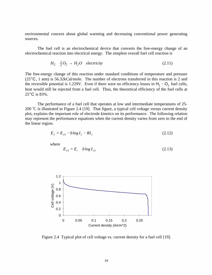
H O H O electricity212 2 2+ → + (2.11)

The free-energy change of this reaction under standard conditions of temperature and pressure(25oC, 1 atm) is 56.32kCal/mole. The number of electrons transferred in this reaction is 2 andthe reversible potential is 1.229V. Even if there were no efficiency losses in H O2 2− fuel cells,heat would still be rejected from a fuel cell. Thus, the theoretical efficiency of the fuel cells at25oC is 83%.

The performance of a fuel cell that operates at low and intermediate temperatures of 25-200 oC is illustrated in Figure 2.4 [19]. That figure, a typical cell voltage versus current densityplot, explains the important role of electrode kinetics on its performance. The following relationmay represent the performance equations when the current density varies from zero to the end ofthe linear region.

E E b I RIf f f f= − −0 log (2.12)

whereE E b If r f0 0= + log (2.13)

0

0.2

0.4

0.6

0.8

1

1.2

0 0.05 0.1 0.15 0.2 0.25Current density (A/cm^2)

Cel

l vol

tage

(V

)

Figure 2.4 Typical plot of cell voltage vs. current density for a fuel cell [19].

19

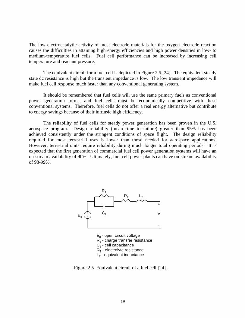
The low electrocatalytic activity of most electrode materials for the oxygen electrode reactioncauses the difficulties in attaining high energy efficiencies and high power densities in low- tomedium-temperature fuel cells. Fuel cell performance can be increased by increasing celltemperature and reactant pressure.

The equivalent circuit for a fuel cell is depicted in Figure 2.5 [24]. The equivalent steadystate dc resistance is high but the transient impedance is low. The low transient impedance willmake fuel cell response much faster than any conventional generating system.

It should be remembered that fuel cells will use the same primary fuels as conventionalpower generation forms, and fuel cells must be economically competitive with theseconventional systems. Therefore, fuel cells do not offer a real energy alternative but contributeto energy savings because of their intrinsic high efficiency.

The reliability of fuel cells for steady power generation has been proven in the U.S.aerospace program. Design reliability (mean time to failure) greater than 95% has beenachieved consistently under the stringent conditions of space flight. The design reliabilityrequired for most terrestrial uses is lower than those needed for aerospace applications.However, terrestrial units require reliability during much longer total operating periods. It isexpected that the first generation of commercial fuel cell power generation systems will have anon-stream availability of 90%. Ultimately, fuel cell power plants can have on-stream availabilityof 98-99%.

+-Eo

R1

C1

RT LT

V

+

-

E0 - open circuit voltageR1 - charge transfer resistanceC1 - cell capacitanceRT - electrolyte resistanceLT - equivalent inductance

Figure 2.5 Equivalent circuit of a fuel cell [24].

20

The high reliability of a fuel cell system will largely result not only from the modularityof the stacks and stack components, but from their lack of highly stressed moving parts operatingunder extreme conditions. It operates under relatively benign conditions, so it can be designedsuch that maintenance is required only at infrequent intervals. A plant could be operated at fullpower during periods of routine maintenance by replacing spare modules. Without spare parts,plants could be designed so that only partial shutdown will be necessary in the event of failure.

Any low-temperature fuel cell system must take several fuel-processing steps to producehydrogen that will be consumed inside the fuel cell stacks. The most effective way to producethe hydrogen is by steam-reforming of hydrocarbon fuels. First, fuel purification to avoidpoisoning of the steam-reforming catalyst is required, which is done by hydrodesulfurization.This is followed by reforming and carbon monoxide (CO) shift reaction to reduce any residualCO values to acceptable levels. The above reactions are endothermic, so they need a net heatinput from the fuel used or from any available heat. High-temperature heat is required for thereforming, typically 750 - 800oC. Unless this heat can be given directly by the waste heat from ahigh-temperature fuel cell, it must be provided by burning excess fuel.

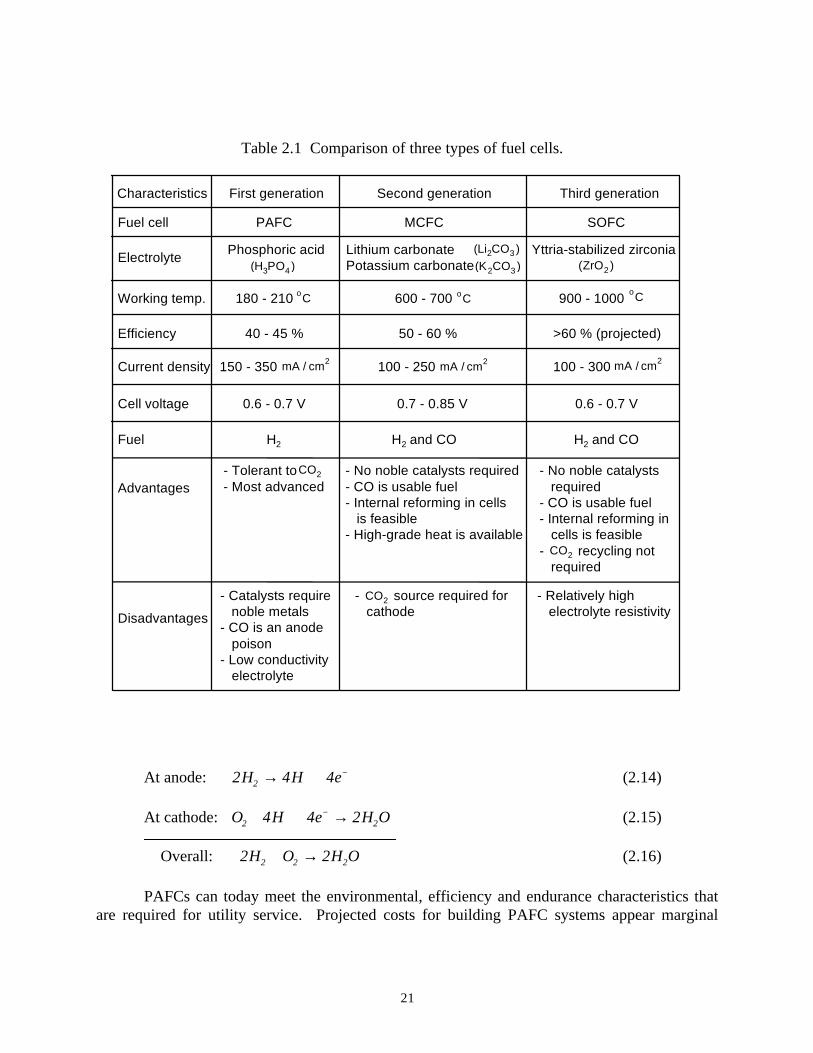
Since the energy crisis of 1973, which was instrumental in the renaissance of fuel cells, ithas been customary to classify fuel cells by the types of electrolyte: alkaline, phosphoric acid,molten carbonate, solid oxide, and solid polymer. The alkaline fuel cell system being used inspace shuttle flights is a strong contender for NASA’s lunar and Mars missions, and the solidpolymer fuel cells are being developed for applications to transportation. Table 2.1 summarizesthe characteristics of three major fuel cell systems that contain great potentials for power utilityapplications.

2.3.2 Phosphoric Acid Fuel Cell (PAFC)

Phosphoric acid technology has moved from the laboratory research and development tocommercial application. The principal obstacle against widespread commercial acceptance iscost. Capital costs of about $2500 - $4000/kW must be reduced to $1000 - $1500/kW if thetechnology is to be accepted in the electric power markets.

The basic cell structure is similar to that of a battery. It consists of an anode, a cathodeand an electrolyte. The anode and cathode are made of a porous graphite substrate treated with aplatinum catalyst, having the surface adjacent to the electrolyte. The electrolyte matrix retainsthe concentrated phosphoric acid and its thickness is in the range between 0.01 and 0.03 cm.The electrolyte matrix has minimum ionic resistance while separating the fuel and oxidant gasstreams.

The PAFC system operates at 180 to 210oC. At lower temperatures, phosphoric acid is apoor ionic conductor. At higher temperatures, material (carbon and platinum) stability becomeslimiting. The chemical reactions occurred at two electrodes are written as follows:

21

Table 2.1 Comparison of three types of fuel cells.

Electrolyte Phosphoric acid ( )H PO3 4

Lithium carbonate Potassium carbonate

( )Li CO2 3

( )K CO2 3

Yttria-stabilized zirconia( )ZrO2

Working temp.

Efficiency

Current density

Cell voltage

Advantages

Disadvantages

180 - 210 600 - 700 900 - 1000

PAFC MCFC SOFC

40 - 45 % 50 - 60 % >60 % (projected)

150 - 350 100 - 250

0.6 - 0.7 V 0.7 - 0.85 V

- Tolerant to- Most advanced

CO2 - No noble catalysts required- CO is usable fuel- Internal reforming in cells is feasible- High-grade heat is available

- No noble catalysts required- CO is usable fuel- Internal reforming in cells is feasible- recycling not required

CO2

- Catalysts require noble metals- CO is an anode poison- Low conductivity electrolyte

- source required for cathode

- Relatively high electrolyte resistivity

CO2

mA cm/ 2 mA cm/ 2

oC oCoC

100 - 300 mA cm/ 2

0.6 - 0.7 V

Fuel H2 H2 and CO H2 and CO

Fuel cell

Characteristics First generation Second generation Third generation

At anode: 2 4 42H H e→ ++ − (2.14)

At cathode: O H e H O2 24 4 2+ + →+ − (2.15)

Overall: 2 22 2 2H O H O+ → (2.16)

PAFCs can today meet the environmental, efficiency and endurance characteristics thatare required for utility service. Projected costs for building PAFC systems appear marginal

22

when compared with costs for alternative power plants. The first utility application would be asa dispersed power generator fueled by a natural gas. However, PAFCs may find applications incoal-fired central-station power plants with coal gasifiers. With the current emphasis oncogeneration, it is also possible that the PAFC’s unique environmental character will lead to itsearly use in applications where its electric and thermal energy can be employed.

2.3.3 Molten Carbonate Fuel Cell (MCFC)

Molten carbonate technology is attractive because it offers several potential advantagesover PAFCs. Carbon monoxide, which poisons the PAFCs, is indirectly used as a fuel inMCFCs. The higher operating temperature of approximately 650oC makes the MCFCs a bettercandidate for combined cycle applications. This technology is on the stage of prototypecommercial demonstrations and main development efforts are focused on large multi-MWcentral-station power plants with a coal gasifier. This is partially due to their high operatingtemperature and the problems inherent in starting (heating) and stopping (cooling) MCFC powerplants. Their capital costs are expected to be lower than those of PAFCs.

The MCFC structure is geometrically very similar to that of the PAFC, but the materialsused are very different from those used in the PAFC. The anode consists of a porous nickeltreated with an insoluble oxide to reduce sintering. The cathode is similar to the anode exceptthat it uses nickel oxide doped with lithium to give electronic conductivity. MCFCs use analkali metal (lithium or potassium) carbonate as the electrolyte. Since these carbonates canfunction as electrolytes only when in the liquid form, the operating temperature should bemaintained above the melting points of the carbonates. The following equations illustrate thechemical reactions that take place inside the cell.

At anode: 2 2 2 2 42 32

2 2H CO H O CO e+ → + +− − (2.17)

and 2 2 4 432

2CO CO CO e+ → +− − (2.18)

At cathode: O CO e CO2 2 322 4 2+ + →− − (2.19)

Overall: 2 22 2 2H O H O+ → (2.20)

2 22 2CO O CO+ → (2.21)

A consequence of these reactions is that CO2 must be recycled from the anode to cathode. Wasteheat from the fuel cell can be available at a relatively high temperature (greater than 500oC),which enables its use in bottoming or industrial heating cycles.

23

A fuel cell system must include fuel conversion process by external or internal reformingfrom sulfur-free hydrocarbon gas to hydrogen-rich gas. For large central MCFC power plants,efficient external reforming may be recommended because of the effects of scale and high-energy efficiency. However, for smaller dispersed units, internal reforming has the advantagesof simplicity and direct use of part of heat generated in the cells.

2.3.4 Solid Oxide Fuel Cell (SOFC)

Solid oxide technology requires very significant changes in the structure of the cell.SOFCs employ a tubular stack configuration. As the name implies, SOFCs use a solid,nonporous metal oxide electrolyte such as stabilized zirconia, so the electrolyte does not need tobe replenished during the operational life of the cells. This simplifies design, operation andmaintenance as well as having the potential to reduce costs. This offers the stability andreliability of all solid-state construction and allows higher temperature operation. The ceramicmake-up of the cell lends itself to cost-effective fabrication techniques.

The anode is typically a porous nickel-zirconia cermet that serves as the electrocatalyst,which can be electronically conductive, allow fuel gas to reach the electrolyte interface, andcatalyze the fuel oxidation reaction. The cathode consists of a discontinuous catalyst layercoated with a porous, doped indium oxide. The cathode must conduct electrons, allow oxygento reach the electrolyte interface, and catalyze the reduction of oxygen to oxide ions. Thechemical reactions inside the cell may be written as follows:

At anode: 2 2 2 422

2H O H O e+ → +− − (2.22)

and 2 2 2 422CO O CO e+ → +− − (2.23)

At cathode: O e O224 2+ →− − (2.24)

Overall: 2 22 2 2H O H O+ → (2.25)

2 22 2CO O CO+ → (2.26)

SOFCs offer advantages similar to those of MCFCs, such as good performance on fuelscontaining hydrogen and carbon monoxide, no need of noble-metal catalysts, and the availabilityof high-grade waste heat. The tolerance to impure fuel streams makes SOFC systems especiallyattractive for utilizing H2 and CO from natural gas steam-reforming and coal gasfication plants.Additionally, they do not suffer the constraint of MCFCs that require a carbon dioxide recycle tothe cathode.

24

2.3.5 Fuel Cell Power Systems

Fuel cells are known to possess a great number of attributes that make them attractive forthe purpose of power generation. The inherent modularity in their production contains thefeature less sensitive to size. It enables them to be added successively. Fuel cells have highefficiency and relatively flat efficiency characteristics that make them useful for part-loadoperation. Fuel cells can utilize a variety of fuels such as natural gas, coal-derived gas, biogasand methanol, and they are able to respond very fast to load changes. Their low noise andemissions and negligible water requirements allow them much more flexibility in siting.Because of those benefits, fuel cells have continuously been under research and developmentdespite their high initial cost right now.

Bell and Hayman [26] reviewed the electric utilities’ efforts to develop fuel celltechnology including the siting and construction of the 4.5MW phosphoric-acid fuel cell (PAFC)demonstrator in New York City. The study suggested that if PAFCs were available with a costof about $400/kW and a heat rate of 9300Btu/kWh, they would be attractive for intermediateduty generation. These fuel cell units would capture about 27% of capacity additions competingagainst nuclear, oil-fired intermediate, and gas turbine units.

Rahman and Tam [1] presented to use fuel cells in coordination with PV systems.Through simulation using actual data from a PV test facility, it was shown that it is feasible touse the PV-fuel cell hybrid system to meet variable loads for either utility or stand-aloneapplications. Operation of the hybrid system overcomes the intermittence problem inherent inPV and makes photovoltaic electric power generation more attractive.

Tam and Rahman [2] proposed an augmented power conditioning subsystem (APCS)applied at central station photovoltaic-fuel cell power plant in order to improve the powersystem performance. By using phase shift control, real and reactive power can be controlledindependently and a variety of operation and control modes are developed for different systemsituations.

Matsumoto et al. [28] discussed a performance model of a molten carbonate fuel cell(MCFC) for any cathode gas composition by single-cell experimental data. The studyinvestigated three different systems (that is, external reforming (ER), direct internal reforming(DIR), and indirect internal reforming (IIR) system) and compared their performances. A DIRsystem can achieve about 6% higher electric power generation efficiency than an ER system, andabout 5% higher than a IIR system.

Hsu et al. [79] is proceeding on development of a hybrid system of a SOFC with a gasturbine, which utilizes the high temperature exhaust gas from the fuel cell system. The hybridsystem is potentially capable of reaching electrical efficiencies around 70% assuming the fuelcell efficiencies from 50 to 55%. They plan to provide the products to customers at a systemprice below $1000/kW.

25

Ruhl et al. [80] have completed preliminary designs and tests for 20 kW SOFC modulesfor stationary distributed generation applications using pipeline natural gas. The system’s NOx

emission level is less than 3 lb/GWh while its efficiencies range from 45 to 50%. Its dynamicresponse capability is less than 4 sec at a load increase from 1 to 100% output, and less than 2msec at a load decrease from 100 to 1%.

2.4 Neural Networks (NNs)

2.4.1 Neural Network Background

Artificial neural networks (ANNs) are information processing systems. Neural networkscan generally be thought of as “ black box” devices that accept inputs and produce outputs.Some of the characteristics that NNs perform include

(i) Classification(ii) Pattern matching(iii) Pattern completion(iv) Noise removal(v) Optimization(vi) Control

Figure 2.6 shows a typical neural network that consists of processing elements (PEs orneurons) and weighted connections. The connection weights which store the information are

x1

x2

xn

y1

y2

yp

z1

z2

zqV W

.

.....

.

..

Input layer

Hiddenlayer

Outputlayer

Figure 2.6 A typical neural network.

26

often determined by a NN learning procedure. The neural network illustrates several importantfeatures such as (i) each PE acts independently of all others, (ii) each PE relies only on localinformation, and (iii) the large number of connections provides a large amount of redundancyand facilitates a distributed representation of information. The first two features allow NNs tooperate efficiently in parallel. The last feature provides NNs with inherent fault-tolerance andgeneralization qualities that are very difficult to obtain from typical computing systems. Inaddition to these features, NNs are able to learn arbitrary nonlinear mappings throughintroduction of nonlinearity in PEs.

PE activation functions map a processing element’s infinite domain to a prespecifiedrange. Although abundant activation functions are possible, the following five functions areusually employed by the majority of NNs:

(i) Linear function (ii) Step function (iii) Ramp function (iv) Sigmoid function (v) Gaussian function

Except for the linear function, all of the functions introduce a nonlinearity in the networkdynamics by limiting the output values within a fixed range.

NNs consist of layer(s) of processing elements interconnected by weighted connections.The arrangement of the PEs, connections, and patterns into a NN is referred to as a topology.Four common NN topologies may be written as

(i) Instars, outstars, and the ADALINE (ii) Single-layer networks (iii) Two-layer networks (iv) Multilayer networks

The instar is the minimal pattern encoding network. The outstar is the dual of the instar and isthe minimal pattern recall NN. The ADALINE (ADAptive LInear NEuron) has the sametopology as the instar, but the weights are adjusted by using the least-mean-square algorithm.One-layer NNs are used to perform pattern processing tasks such as pattern completion, noiseremoval, and optimization and two-layer NNs are used for pattern matching and patternclassification. Application fields of multilayer NNs are pattern classification, pattern matching,and function approximation. For the question of how many layers are enough for a givenproblem, it was proven that three layers (one hidden layer) are sufficient to perform anynonlinear mapping to any desired degree of accuracy. Although this is a very important result, itstill does not indicate the proper number of PEs in hidden layers.

27

The most appealing quality of NNs is their ability to learn. Learning is defined as achange in connection weight values that results in capture of information. All learning methodscan be classified into two categories: supervised and unsupervised learning. Supervised learningis a process that requires an external teacher whereas unsupervised learning is a process thatincorporates no external teacher and relies upon only local information during the entire learningprocess. The six most famous learning methods are listed as

(i) Hebbian learning (ii) Differential Hebbian learning (iii) Competitive learning (iv) Two-layer error correction learning (v) Multilayer error backpropagation learning (vi) Stochastic learningTable 2.2 describes five key attributes of the neural network learning algorithms mentionedabove.

2.4.2 NN Applications to Power Systems

Applications of artificial neural networks to power systems have advanced rapidly inrecent years. NNs have been widely applied for solving various power system problemsincluding security assessment [60, 63, 68], stability analysis [61, 64, 67], tuning of power systemstabilizers [62, 72], generator shedding problem [65], fault identification [66, 71], unitcommitment [69], subsynchronous resonance oscillation [70], VAR control [73], loadforecasting [74], economic/

Table 2.2 Key attributes of the principal learning procedures [59].

Hebbian learning

Differential Hebbian learning

Competitive learning

Two-layer error correction

Error backpropagation

Stochastic learning

Fast On-line Unsupervised Linear Structural

Fast On-line Unsupervised Linear Structural

Slow On-line Unsupervised Linear Structural

Slow Off-line Supervised Linear Both

Very slow Off-line Supervised Nonlinear Both

Extremely slow Off-line Supervised Nonlinear Structural

Learning algorithm

Learning On-line/ Supervised/ Linear/ Structural/

Time Off-line Unsupervised Nonlinear Temporal

28

environmental dispatch [75], and voltage stability assessment [76]. The success of these worksresults from the fact that NNs are capable of solving a complicated problem in an efficient wayby performing parallel processing on the information distributed over a number of neurons(processing elements).

Chen and Hsu [61] developed a new learning method of multilayer NNs (one hiddenlayer) for the steady-state stability analysis of a synchronous generator. The inputs of the NNare the real power output and power factor of the generator and power system stabilizer (PSS)parameters. The output of the network provides the information on steady-state stability. Theirlearning algorithm is that the outputs of hidden layer neurons are binary-valued (0 or 1)depending upon the inputs, and then the value of the output neuron is decided as the “ BooleanAND” operation of the binary hidden-layer outputs. By the computer simulation, it is found thatthe proposed learning method converges faster and its misclassification rate is lower than theerror backpropagation method. The misclassification rate of the proposed method is 3.5% on 10minutes of learning time.

Ikenono and Iwamoto [64] presented a generalized online technique for transient stabilityanalysis using the backpropagation algorithm. The NN consists of one input layer, one hiddenlayer and one output layer. The numbers of neurons in the input, hidden and output layers are32, 15, and 1 respectively. The output neuron denotes the critical breaker clearing time and theinput neurons include magnitude of bus voltage, angle of bus voltage, generator output power,load power, inertia constant of generator and existence of alteration in system configuration.Simulation results indicate that the proposed technique gives desirable solution if criticalclearing time is short, but when critical clearing time is rather long, the proposed method givessome results requiring a longer time.

Hsu and Chen [62] proposed a new approach using an ANN for adapting PSSparameters. It is desirable to adapt the PSS parameters in real time based on generator loadingconditions in order to have good damping characteristics over a wide range of operatingconditions. They used a multilayer feedforward NN (two hidden layers) with the errorbackpropagation learning rule. The inputs to the NN contain generator real power output andpower factor, which characterize generator operating conditions. The outputs of the network arethe desired PSS parameters. It is concluded from the simulation results that the generator canmaintain good damping features over a wide range of operating conditions when the PSSparameters are adapted by the ANN. The generator with fixed PSS parameters does not yieldsatisfactory dynamic responses when the operating condition is severely perturbed.

El-Keib and Ma [76] investigated voltage stability problem resulting from system heavyloading and proposed a multilayer feedforward ANN with error backpropagation learning forcalculation of voltage stability margins. The proposed method uses an energy function, derivedfrom a vector integration of the real and reactive power mismatch equations between a stableequilibrium point and an unstable equilibrium point, to provide a quantitative measure of system

29

vulnerability to voltage instability. Sensitivity of the energy margin with respect to systemvariables provides information regarding the most effective direction to steer the system tomaximize voltage stability. As input candidates to the NN, real and reactive powers at all busesas well as real and reactive power outputs of all generators are applied. Then a reasonablenumber of inputs are selected by the sensitivity method. The analysis reveals that the systemexhibits quite different response scenarios as system loading conditions vary. Moreover, thesensitivity method causes the NN to produce less accurate estimation of voltage stability marginwhen operating states are near the collapse point.

Sidhu and Ao [77] proposed an adaptive loss evaluation algorithm based on NN usingbackpropagation for power transmission systems. A three-layer feedforward network isemployed because it can model complex mapping functions reasonably well. Real and reactivepowers of generators and loads, as well as voltage magnitudes at voltage-controlled buses arechosen as inputs to the NN, and total system losses are the output. The computed capacity lossesfrom the NN are as close as those obtained by load flow studies; the maximum error is 1.8%.The proposed network can be used to predict capacity and energy losses as a part of off-line loadforecasting. For on-line applications, it can be used to monitor the actual capacity losses in thesystem.

King et al. [75] applied the Hopfield neural network to optimal economic/environmentaldispatch of thermal generating units in an electric power system. A multi-objective function isadopted to minimize both the total fuel cost and NOx/SO2 emissions of thermal units. Theyintroduced an energy function of state variables that maps the economic/environmental dispatchproblem to the Hopfield domain. The Hopfield model, a single layer recursive NN, is createdwith N neurons, one for each generating unit. The output value of each neuron represents thegeneration value of each unit. Computation results indicated that the cost of generation increasesas emission levels decrease and including transmission losses in the dispatch problemcomplicates obtaining the optimal solution.

2.5 Power Conditioning Subsystems (PCSs)

2.5.1 Background Information

Photovoltaic or fuel cell power systems, which generate power as dc electricity, requirepower conversion devices from dc to ac in order to provide power to the transmission anddistribution network of a utility grid. There are other applications, where it is necessary to beable to control power flow in both directions between the ac and dc sides. Examples of suchapplications are converters in battery and supermagnetic energy storage or high-voltage dcpower transmission.

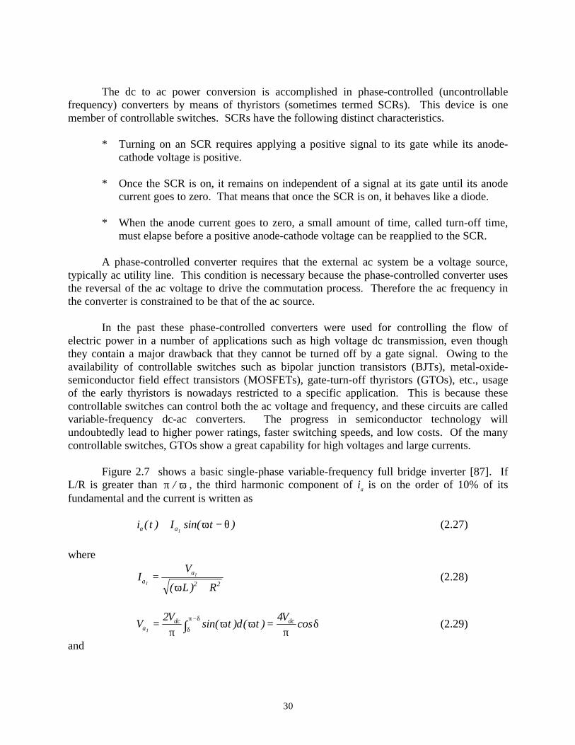
30

The dc to ac power conversion is accomplished in phase-controlled (uncontrollablefrequency) converters by means of thyristors (sometimes termed SCRs). This device is onemember of controllable switches. SCRs have the following distinct characteristics.

* Turning on an SCR requires applying a positive signal to its gate while its anode-cathode voltage is positive.

* Once the SCR is on, it remains on independent of a signal at its gate until its anodecurrent goes to zero. That means that once the SCR is on, it behaves like a diode.

* When the anode current goes to zero, a small amount of time, called turn-off time,must elapse before a positive anode-cathode voltage can be reapplied to the SCR.

A phase-controlled converter requires that the external ac system be a voltage source,typically ac utility line. This condition is necessary because the phase-controlled converter usesthe reversal of the ac voltage to drive the commutation process. Therefore the ac frequency inthe converter is constrained to be that of the ac source.

In the past these phase-controlled converters were used for controlling the flow ofelectric power in a number of applications such as high voltage dc transmission, even thoughthey contain a major drawback that they cannot be turned off by a gate signal. Owing to theavailability of controllable switches such as bipolar junction transistors (BJTs), metal-oxide-semiconductor field effect transistors (MOSFETs), gate-turn-off thyristors (GTOs), etc., usageof the early thyristors is nowadays restricted to a specific application. This is because thesecontrollable switches can control both the ac voltage and frequency, and these circuits are calledvariable-frequency dc-ac converters. The progress in semiconductor technology willundoubtedly lead to higher power ratings, faster switching speeds, and low costs. Of the manycontrollable switches, GTOs show a great capability for high voltages and large currents.

Figure 2.7 shows a basic single-phase variable-frequency full bridge inverter [87]. IfL/R is greater than π ω/ , the third harmonic component of ia is on the order of 10% of itsfundamental and the current is written as

i t I ta a( ) sin( )≅ −1

ω θ (2.27)

where

IV

L Ra

a1

1

2 2=

+( )ω (2.28)

V V t d t Va

dc dc1

2 4= =−∫π

ω ωπ

δδ

π δ sin( ) ( ) cos (2.29)

and

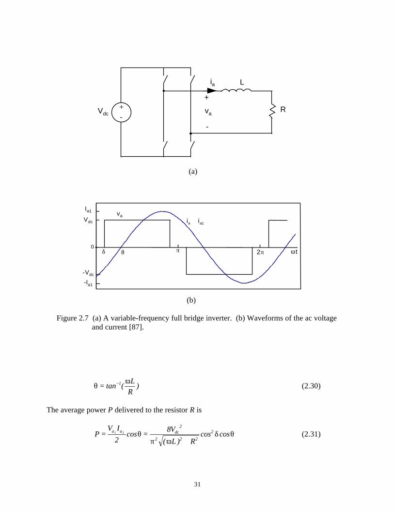
31

+-

L

Rva

ia

Vdc

+

-

(a)

0

Ia1

Vdc

-Vdc

-Ia1

va

δ θ π 2π ωt

i ia a≅ 1

(b)

Figure 2.7 (a) A variable-frequency full bridge inverter. (b) Waveforms of the ac voltage and current [87].

θ ω= −tan ( )1 LR

(2.30)

The average power P delivered to the resistor R is

PV I V

L Ra a dc= =

+1 1

28 2

2 2 2

2cos( )

cos cosθπ ω

δ θ (2.31)

32

From this analysis the power depends on δ , and therefore the power can be controlledonly by varying δ or Vdc. This is because the power factor is fixed in the passive load of Figure2.7 (a). If the resistive load in Figure 2.7 is replaced with an ac voltage source, θ in addition toδ can be used as a control variable.

2.5.2 PCU Applications to Renewable Power Sources

Large scale grid-connected photovoltaic or fuel cell power plants require powerconversion from the dc generated from the power plants to the ac of a three-phase power utilitynetwork. Efficient control of dc to ac power conversion devices, design of a new inverter circuitfor photovoltaic energy feedback into a utility grid, and modeling of an inverter with differenttypes of commutation are discussed. Michaels et al. [55] presented simulation techniques forline-commutated and self-commutated three-phase bridge inverters. They represented thesystem by different sets of differential equations depending upon the states of the switches in thecircuit. As a result, they have found that the self-commutated inverter is more suitable for theapplication to a fuel cell system than the line-commutated inverter. They, finally, proposed thatthis kind of inversion device should have features such as high conversion efficiency, low capitaland operating costs, compatibility with utility system interface, and operating flexibility forcontrol of voltage and real/reactive power.

Dugan et al. [44] studied harmonic distortions in voltage and reactive power correctionfrom 6.6kW line-commutated inverters in 100 photovoltaic house subdivision, which isequivalent to approximately 7% penetration on the 10MVA distribution feeder. Under commonconditions the total harmonic distortion (THD) caused by the inverters is around 2-3%, andunder the worst conditions it reaches 6.2% on one feeder and 4.8% on the other. The studyindicated that the THD levels are strongly influenced by the power factor correction capacitorson the distribution feeder, and each line-commutated inverter consumes up to 4kVar of reactivepower at peak output.

Boegli and Ulmi [8] realized a new regulated utility interactive inverter for directresidential photovoltaic energy feedback to a public utility grid. A modulated buck converterconverts the photovoltaic dc current to a rectified 50-Hz sine wave current and the followingself-commutated half-bridge inverter generates a 50-Hz sine wave current. It is, then, fed intoone phase of the public utility grid. The new inverter needs only three power transistor switchesand a transformer for isolation between the PV array and the grid. The yearly overall efficiencyof the 1-kW prototype is 88% and the total harmonic distortion is 1% at 1kW.

Wasynczuk [5, 6] described simplified computer models of three-phase line-commutatedand self-commutated utility interactive photovoltaic inverter systems for applications to transientstability analysis. The computer simulation indicated that the simplified models are reasonably

33

accurate when used to predict the PV system response following step changes in the inverterdelay angle, rapid decreases or increases in solar insolation and step changes in ac voltagemagnitude or phase.

R. Naik [89] presented a new topology for interfacing of PV, wind-electric and fuel-cellsystems with a utility grid. The interface consists of a 3-phase dc-ac line-commutated inverterand dc-dc converter. The firing angle of the 3-phase inverter is kept at a constant value and thepower flow from the dc source to the utility is controlled by the dc-dc converter. A constant-extinction angle control scheme is used, which is common in converters for the HVDCtransmission systems. The total harmonic distortion (THD) in line currents is 3.9% at simulationand that is 5.9% at experiment results.

W. Shireen and M.S. Arefeen [90] proposed a modified inverter switching technique forthe interface with a utility grid such that the ac output of the 3-phase pulse-width modulation(PWM) inverter becomes immune to fluctuations in the unregulated dc input, such as battery,fuel cells, PV cells, etc. The proposed method is a feedforward approach to suitably alter themodulating function for inverter switching control to counter the fluctuation in the input dcvoltage. If the input voltage increases, the width of the PWM pulses decrease and if the inputvoltage decreases, the width of the PWM pulses increase. The response time for accommodatinginput voltage variation is limited by the delay of the control circuit. The experiment resultsreveal that the lower order harmonics of the output voltage are effectively canceled.

34

CHAPTER 3

BATTERIES OR FUEL CELLS FOR PV POWER BACKUP

As energy storage devices, batteries continue to be applied to electric power utilities fordrawing benefits of peak shaving and load leveling. Battery energy storage facilities provide theutilities additional dynamic benefits such as voltage and frequency regulation, load following,spinning reserve, and power factor correction [34, 38]. Applications of the storage batteries topower systems are predicted to grow in the future due to those benefits coupled with the abilityto provide peak power.

Fuel cell power generation is another attractive option for providing power for electricutilities and commercial buildings because of its high efficiency and environmentally benignfeature. This type of power production is especially economical (i) where potential users arefaced with high cost in electric power generation from coal or oil, (ii) where environmentalconstraints are stringent, or (iii) where load constraints of transmission and distribution systemsare so tight that their new installations are not possible.

Both batteries and fuel cells have their own unique contributions to electric powersystems as discussed above. Those two power sources also contain a great potential to back upsevere PV power fluctuations under inclement weather conditions. In this chapter comparisonbetween batteries and fuel cells is carried out in detail only for their PV power backup options,so their common attributes and different attributes will be discussed.

3.1 Common Attributes

Photovoltaic power outputs vary depending mainly upon solar insolation and celltemperature. Since control of the ambient weather conditions is beyond human beings’capability, it is almost impossible for human operators to control the PV power itself. Thus, a

35

PV power generator may sometimes experience sharp output power fluctuations owing tointermittent weather conditions, which causes control problems such as load frequency control,generator voltage control and even system stability analysis.

There is, therefore, a need for backup power facilities in the PV power generation. Asmentioned in Chapter 1, batteries and fuel cells are the most likely technologies to provide thePV system with backup power because these two backup power sources contain some distinctfeatures in common. Those characteristics are listed below.

- Fast load-response capability: Fuel cells and batteries are able to respond very fast to loadchanges because their electricity is generated by chemical reactions. A 14.4kW lead-acid battery running at 600A has maximum load gradient of 300 A/sec [31]. Aphosphoric-acid fuel cell system can match a demand that varies by more than half itsrated output within 0.1 second [78]. The dynamic response time of a 20kW solid-oxidefuel cell power plant is less than 4 second when a load increases from 1 to 100%, and itis less than 2 msec when a load decreases from 100 to 1% [80].

- Modularity in production: Factory assembly of standard cell units provides fuel cell andbattery power plants with short lead-time from planning to installation. This modularproduction enables them to be added in discrete increments of capacity, which allowsbetter matching of the power plant capacity to expected load growth. In contrast, theinstallation of a single large conventional power plant may produce excess capacity forseveral years, especially if the load growth rate is low.

- Highly reliable sources: Due to their multiple parallel modular units and absence ofelectromechanical rotating masses, fuel cell and battery power plants are more reliablethan any other forms of power generation. Fuel cells are expected to attain aperformance reliability near 85% [91]. Consequently, a utility that installs a number offuel cell or battery power plants is able to reduce its reserve margin capacity whilemaintaining a constant level of the system reliability.

- Flexibility in site selection (Environmental acceptability): The electrochemical conversionprocesses of fuel cells and batteries are very quiet because they do not have any majorrotating masses. External water requirement for their operation is, if any, very littlewhile conventional power plants require massive amount of water for system cooling.Therefore, they can reduce or eliminate water quality problems created by theconventional plants’ thermal discharges. Air pollutant emission levels of fuel cells andbatteries are none or very little. Emissions of SO2 and NOx in the fuel cell power plantare 0.003 lb/MWh and 0.0004 lb/MWh respectively. Those values are projected to beabout 1,000 times smaller than those of fossil-fuel power plants since fuel cells do notrely on a fuel-burning process [91]. These environmentally benign characteristicsmake it possible for those power plants to be located close to load centers in urban andsuburban area. It can also reduce energy losses and costs associated with transmission

36

and distribution equipment. These siting near load centers may also reduce thelikelihood of system blackouts.

3.2 Different Attributes

Electric current is produced in a storage battery by chemical reactions. The samechemical reactions take place in a fuel cell, but there is a difference between them with respect tofuel storage. In storage batteries chemical energy is stored in the positive/negative electrodes ofthe batteries. In fuel cells, however, the fuels are stored outside the cells and need to be fed intothe electrodes continuously when the fuel cells are required to generate electricity. Otherdetailed comparison between battery backup and fuel cell backup for PV power supplement ismade in the following sections.

3.2.1 Efficiency

Power generation in fuel cells is not limited by the Carnot Cycle in the view that theydirectly convert available chemical free energy to electrical energy rather than going throughheat exchange processes. Thus, it can be said that fuel cells are a more efficient powerconversion technology than the conventional steam-applying power generations. Figure 3.1illustrates energy conversion processes for a conventional power generator and a fuel cell.Whereas the fuel cell is a one-step process to generate electricity, the conventional powergenerator has several steps for electricity generation and each step requires a certain amount ofenergy loss.

Fuel cell power systems have around 40-60% efficiencies depending on the type ofelectrolytes. For example, the efficiencies of phosphoric-acid fuel cells and molten-carbonatefuel cells are 40-45% and 50-60%, respectively. Furthermore, the fuel cell efficiency is usuallyindependent of size; small power plants operate as efficiently as large ones.

Battery power systems themselves have high energy efficiencies of nearly 80%, but theiroverall system efficiencies from raw fuel (mostly coal or nuclear) through the batteries toconverted ac power are reduced to below 30%. This is because energy losses take placewhenever one energy form is converted to another. For this calculation, a 35% of efficiency wasassumed for electricity generation from coal or nuclear power stations.

3.2.2 Capacity Variation

The capacity of a fuel cell is expressed in watts (W), whilst that of a storage battery isrepresented in ampere-hours (Ah) or watt-hours (Wh). A battery with a rated capacity of 100Ah

37

ChemicalEnergy

Heat

Mechanical Motion

Electricity

ChemicalEnergy

Electricity

Electricity

ChemicalEnergy

Fuel cellsConventional power generators

Batteries

Figure 3.1 Comparison of energy conversion processes [78].

at a 10-hr discharge rate can supply 10A for 10 hours. At discharge rates in excess of 10A, thebattery will provide less than 100 Ah. At less than 10A of discharge rates, the battery willprovide more that 100 Ah. Thus, in specifying the capacity of a battery, it is necessary to notethe time rate of discharge.

As the battery discharges, its terminal voltage, the product of the load current and thebattery internal resistance (Rbat), gradually decreases. The fall of the terminal voltage ondischarge is due to its internal resistance. When Rbat is constant at given cell temperature andstate of discharge, the terminal voltage drop is directly proportional to the load current.However, the internal resistance of a battery varies with its cell temperature and state ofdischarge. The resistance increases with both fall in cell temperature and depth of discharge.

38

The decrease in battery voltages with increasing discharge currents is clearly seen inFigure 3.2 [14]. There is also a reduction in battery capacity with increasing rate of discharge.At 1-hr discharge rate, the available capacity is only 55% of that obtained at 20-hr rate. This isbecause there is insufficient time for the stronger acid to replace the weak acid inside the batteryas the discharge proceeds. Capacity variations at different rates of discharge can be calculatedfrom the curves in Figure 3.2, and is shown in Table 3.1 [14].

For fuel cell power systems, they have equally high efficiency at both partial and fullloads as can be seen in Figure 3.3 [78]. The customer’s demand for electrical energy is notalways constant. So for a power utility to keep adjustment to this changing demand, either largebase-load power plants must sometimes operate at part load, or smaller peaking units must beused during periods of high demand. Either way, efficiency suffers and pollution increases.Fuel cell systems have a greater efficiency at full load and this high efficiency is retained as loaddiminishes, so inefficient peaking generators may not be needed.

3.2.3 Flexibility in Operation

Fuel cells have an advantage over storage batteries in the respect of operationalflexibility. Batteries need several hours to be taken for recharging after they are fully

10

11

12

13

4 8 12 16 200

Bat

tery

Vol

tage

[V]

Time [hrs]

2A3.7A6.5A22A

Figure 3.2 Voltage characteristics of a battery at various discharge rates [14].

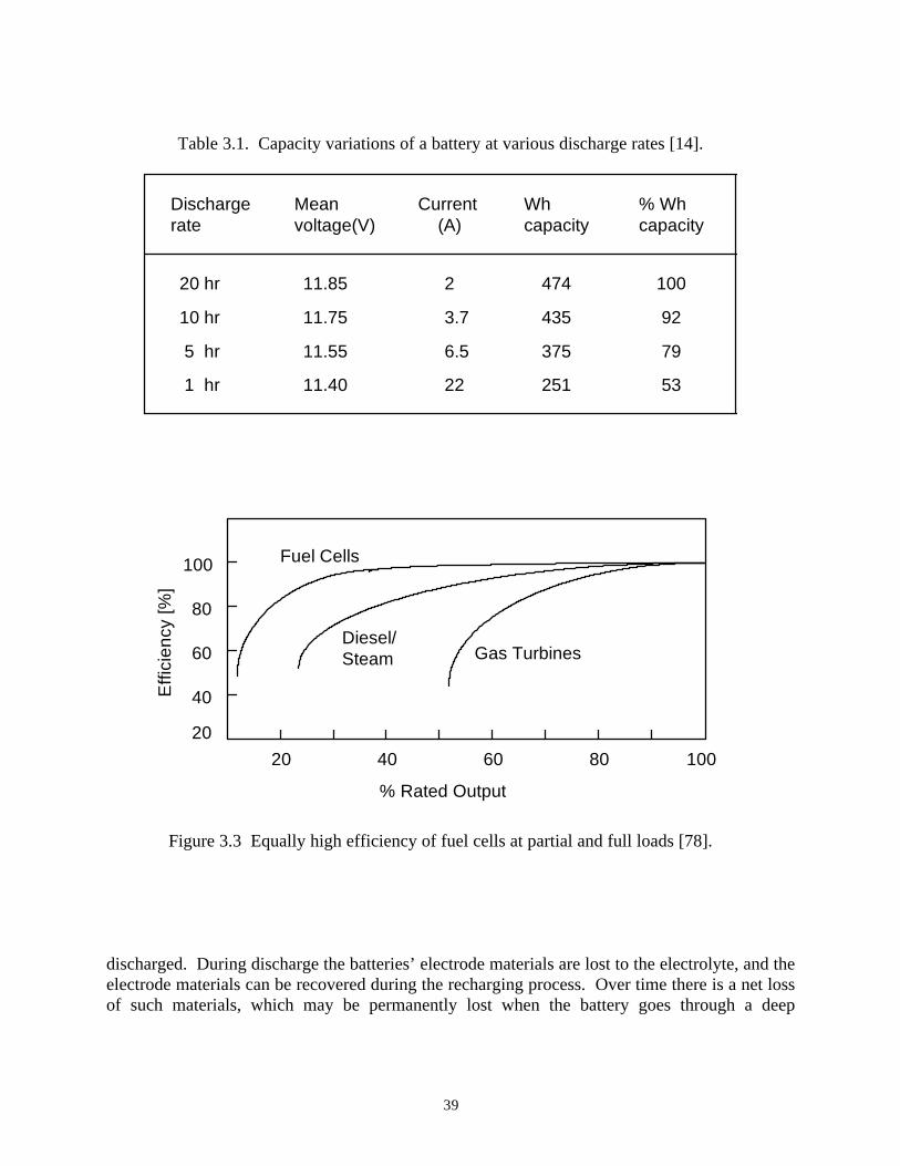
39

Table 3.1. Capacity variations of a battery at various discharge rates [14].

Dischargerate

Meanvoltage(V)

Whcapacity

% Whcapacity

20 hr

10 hr

5 hr

1 hr

11.85

11.75

11.55

11.40

474

435

375

251

100

92

79

53

Current (A)

2

3.7

6.5

22

20

40

60

80

100

20 40 60 80 100

% Rated Output

Effi

cien

cy [%

]

Fuel Cells

Gas TurbinesDiesel/Steam

Figure 3.3 Equally high efficiency of fuel cells at partial and full loads [78].

discharged. During discharge the batteries’ electrode materials are lost to the electrolyte, and theelectrode materials can be recovered during the recharging process. Over time there is a net lossof such materials, which may be permanently lost when the battery goes through a deep

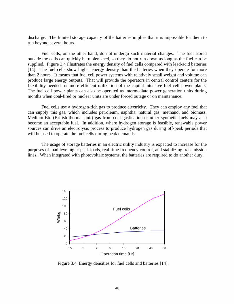
40

discharge. The limited storage capacity of the batteries implies that it is impossible for them torun beyond several hours.

Fuel cells, on the other hand, do not undergo such material changes. The fuel storedoutside the cells can quickly be replenished, so they do not run down as long as the fuel can besupplied. Figure 3.4 illustrates the energy density of fuel cells compared with lead-acid batteries[14]. The fuel cells show higher energy density than the batteries when they operate for morethan 2 hours. It means that fuel cell power systems with relatively small weight and volume canproduce large energy outputs. That will provide the operators in central control centers for theflexibility needed for more efficient utilization of the capital-intensive fuel cell power plants.The fuel cell power plants can also be operated as intermediate power generation units duringmonths when coal-fired or nuclear units are under forced outage or on maintenance.

Fuel cells use a hydrogen-rich gas to produce electricity. They can employ any fuel thatcan supply this gas, which includes petroleum, naphtha, natural gas, methanol and biomass.Medium-Btu (British thermal unit) gas from coal gasfication or other synthetic fuels may alsobecome an acceptable fuel. In addition, where hydrogen storage is feasible, renewable powersources can drive an electrolysis process to produce hydrogen gas during off-peak periods thatwill be used to operate the fuel cells during peak demands.

The usage of storage batteries in an electric utility industry is expected to increase for thepurposes of load leveling at peak loads, real-time frequency control, and stabilizing transmissionlines. When integrated with photovoltaic systems, the batteries are required to do another duty.

0

20

40

60

80

100

120

140

0.5 1 2 5 10 20 40 60

Operation time [Hr]

Wh/

kg

Batteries

Fuel cells

Figure 3.4 Energy densities for fuel cells and batteries [14].

41

It is to suppress the PV power fluctuations due to the changes of solar intensity and celltemperature. The fact that the PV power outputs change sharply under inclement weatherconditions makes it hard to decide the capacity of the battery power plants since theirdischarging rates are not constant. For a lead-acid battery, the most applicable batterytechnology for photovoltaic applications to date, the depth of discharge should not exceed 80%because the deep discharge cycle reduces its effective lifetime. In order to prevent the deepdischarge and to supplement varying the PV powers generated on inclement weather days, thebattery capacity must be large. From Figure 3.5, that shows two different PV power variations,the dotted curve requires a larger battery capacity than the other curve. Moreover, the largebattery capacity is usually not fully utilized, but for only several days.

Fuel cells integrated with photovoltaic systems can provide smoother operation. The fuelcell system is capable of responding quickly enough to level the combined power output of thehybrid PV-fuel cell system in case of severe changes in PV power output. Such a fast time-response capability allows a utility to lower its need for on-line spinning reserve. The flexibilityof longer daily operation also makes it possible for the fuel cells to perform more than the rolesof gas-fired power plants. Gas turbines are not economical for a purpose of load followingbecause their efficiencies become lower and operating costs get higher at less than full loadconditions.

-50

0

50

100

150

200

250

300

350

0 4 8 12 16 20

Time [hr]

PV

pow

er o

utpu

t [W

]

Figure 3.5 PV power variations requiring different battery capacities.

42

3.2.4 Cost

The history of fuel cell equipment costs has shown that the price of fuel cells has droppedsignificantly as the commercial market grows and the manufacturing technology becomesmature. Initial cost of phosphoric acid fuel cell power plants was $5,500/kW and the currentsystem cost is about $3,000/kW [84]. This cost is expected to decrease further to around$1,500/kW by the turn of the century.

The cost of electricity to a utility customer who purchases a fuel cell power system at$1,500/kW is 9-10cents/kWh until the short-term loan is retired, and then it falls to about5cents/kWh. Under longer-term financing that is typical of utility industries, the $1,500/kWelectricity production cost of fuel cell power plants is approximately 7cents/kWh [85].

Batteries have a different cost notation since their capacity is represented in watt-hours.A lead-acid battery power plant has currently the lowest battery cost at around $150/kWhbecause it has been the longest and most fully developed battery technology. The battery cost isprojected to reduce to $100/kWh in the future. Nickel-cadmium (NiCd) batteries are 4 to 5times more expensive than the lead-acid types. Once the NiCd batteries are fully mature, theirprice will drop but they will not be as low as the lead-acid ones because of the raw material cost.

3.2.5 Environmental Externality

During their life cycle operation, fuel cell power plants produce environmentalexternalities in the process of fuel reforming. However, storage batteries themselves do notcontain any environmental impacts even though the battery charging sources produce variousemissions and solid wastes. A fuel cell power system emits by far less SO2, NOx and otherparticulates in the fuel reforming process compared to conventional fossil fuel power plants.The amount of CO2 emissions from the fuel cell system is similar to that from conventionalfossil-fuel power plants, but the fuel cell system’s high efficiency ranging from 40% to 60%results in lower CO2 emissions.

Batteries themselves do not produce any emissions during their operation period even ifthe power sources providing the batteries with charging power usually at off-peak time generateseveral chemical emissions and solid wastes. The batteries displace power generation rather thanreplace it. Therefore, the batteries’ environmental impacts should be computed based on thebaseload fuel mix used to charge the batteries.

For instance, the CO2 emissions from fuel cell power plants were calculated as 376.43kgCO2/MWh in Appendix C, where the efficiencies of the fuel reformer and the power plant areassumed to be 95% and 45% respectively. For batteries, the CO2 emissions of the power sourcesthat charge the batteries at off-peak should be computed. When the fuel mix during a charging

43

period of the batteries is supposed to be 40% of nuclear power and 60% of coal power, then thebatteries’ CO2 emission rate would be 714.3 kgCO2/MWh. The results in Appendix A are usedin this calculation.

When fuel cell power plants are to be dismantled at the end of their commission, they donot exhibit any detrimental impacts on environment and no specific hazards are encountered.Component recovery rather than waste disposal is likely to be the issue. In phosphoric-acid fuelcells, nickel from the fuel reformer catalyst and platinum from the anode and cathode willrequire recovery. For molten-carbonate fuel cells, nickel from both the electrodes and thereforming catalysts can be recovered. In solid-oxide fuel cells, nickel and zirconium-containingceramic components are likely to be recovered.

However, for battery power plants a significant amount of care is required to be taken oftheir disposal to prevent toxic materials from spreading around. All batteries that arecommercially viable or under development for power system applications contain hazardous andtoxic materials such as lead, cadmium, sodium, sulfur, bromine, etc. Since the batteries have noapparent salvage value and must be treated as hazardous wastes, disposal of spent batteries is anissue. Recycling batteries is encouraged rather than placing them in a landfill. One methodfavoring recycling of spent batteries is regulation. Thermal treatment for the lead-acid andcadmium-containing batteries is needed to recover lead and cadmium. Sodium-sulfur and zinc-bromine batteries are also required to be treated before disposal.

3.3 Summary

Both batteries and fuel cells are able to respond very fast to system load changes becausethey produce electricity by chemical reactions inside them. Their fast load-response capabilitycan nicely support the sharp PV power variations resulted from ambient weather changes. Thesetwo PV power backup technologies also contain some excellent attributes in common, such asmodular production, high reliability and flexibility in site selection.

However, there are subtle different attributes between batteries and fuel cells when theyare applied to a PV power backup option. Power generation in fuel cell power plants is notlimited by the Carnot Cycle, so they can achieve high power conversion efficiency. (Theirtheoretical maximum efficiency is 83%.) Even taking into account the losses due to activationoverpotential and ohmic losses, the fuel cells still have high efficiencies from 40% to 60%. Forexample, efficiencies of PAFCs and MCFCs are 40-45% and 50-60% respectively. Batterypower plants, on the other hand, themselves have high energy efficiency of nearly 80%, but theoverall system efficiency from raw fuel through the batteries to the converted ac power isreduced to about 30%.

44

A battery’s terminal voltage gradually decreases as the battery discharges due to aproportional decrease of its current. A battery capacity reduces with increasing rate ofdischarge, so its full capacity cannot be utilized when it discharges at high rates. On the otherhand, fuel cell power plants have equally high efficiency at both partial and full loads. Thisfeature allows the fuel cells to be able to follow a changing demand without losing efficiency.

The limited storage capacity of batteries indicates that it is impossible for them to runbeyond several hours. The batteries when fully discharged need several hours to be recharged.For its use in PV power connections, it is as hard as forecasting the weather to compute the exactcapacity of the batteries. In order to prevent the batteries’ deep discharge and to supplement thevarying PV powers on some inclement weather days, the battery capacity should be large, butthat large capacity is not fully utilized on shiny days. For fuel cells, they do not contain such anoperational time restriction as long as the fuel can be supplied. Thus, the fuel cell power plantscan provide operational flexibility with the operators in central control centers by utilizing themefficiently. As intermediate power generation sources, fuel cell power plants may replace coal-fired or nuclear units under forced outage or on maintenance.

Storage batteries possess several benefits in peak shaving and load leveling for a powersystem operation. For those objectives, the batteries’ discharge rate is nearly constant at ratedvalue and their capacity can be fully utilized when designed optimally. The battery operationseems to be periodical every day; that is, it charges at system’s off-peak and discharges at peaktime. Therefore, the batteries can do a great job for those purposes. For the PV power backupthe batteries’ discharge rate is irregular and their full capacity may usually not be consumed. So,it is difficult to design an optimal capacity of the battery systems for support of the PV powervariations and to economically operate them. Instead of batteries fuel cell power plants exhibitdiverse operational flexibility for either a PV power backup or a support of power systemoperation.

45

CHAPTER 4

DESCRIPTION OF PV-FUEL CELL HYBRID SYSTEM

4.1 Overall View of the PV-Fuel Cell Power Plant

Figure 4.1 illustrates a simplified diagram of a grid-connected PV-fuel cell hybrid powerplant including two loops of controllers; that is, a neural network controller for MPPT and areal/reactive power controller. The hybrid system consists of a photovoltaic array, a fuel cellplant and fuel reformer, and power conditioning subsystems (PCSs). The photovoltaic generatoroperates independently and is controlled to produce maximum available solar power. Powerinverters in the PCS fulfill dc-ac power conversion by turning on and off switches according to acertain switching scheme. The neural network controller generates optimal switching signals tothe power inverters for the PV array to always track the maximum power points.

The PV array, composed of a set of series-parallel connected solar cells, generates a dcpower that is then converted to a useful ac power by the PCS. It acts as the interface betweenthe photovoltaic power system and the ac utility grid. The output ac power of the PCS isprovided to the utility grid through the transformer and interconnecting reactance. The neuralnetwork controller for MPPT receives as inputs the available insolation level and celltemperature. Then it sends out output switching signals to the inverters connected to the PVs,and therefore the photovoltaic generator always generates the maximum available solar power.

The fuel cell power generator is used as a supplement to the PV power plant. The fastramping capability of the fuel cell power generation makes it be able to smooth out the PVpower fluctuations owing to intermittent insolation changes. The other duty of the fuel cellpower generator is to meet required real and reactive power demands of a power utility. Thatduty is performed in this study by the real/reactive power controller (RRPC), which consists ofPI-type controllers. The fuel cell’s capability for fast dynamic response is able to control realand reactive powers efficiently so that it would enhance power system stability.

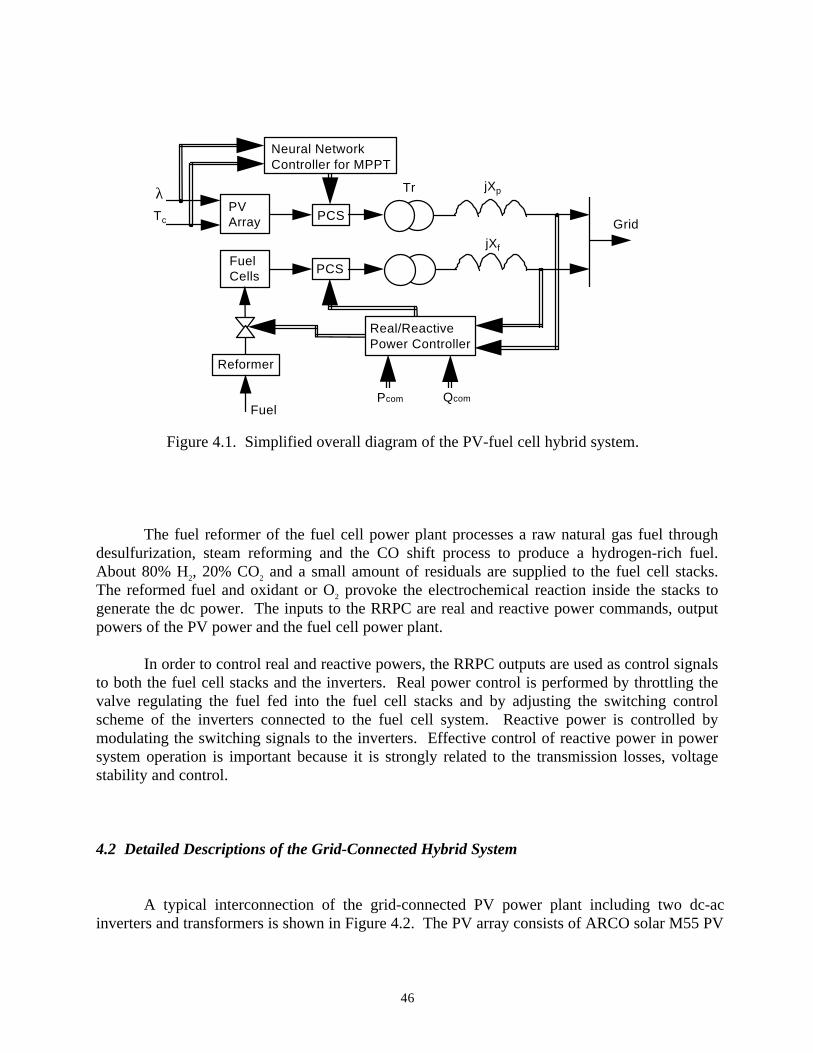
46

PVArray

FuelCells

PCS

Neural Network Controller for MPPT

Real/ReactivePower Controller

jXp

jXf

Tr

Reformer

Pcom Qcom

Grid

Fuel

PCS

λTc

Figure 4.1. Simplified overall diagram of the PV-fuel cell hybrid system.

The fuel reformer of the fuel cell power plant processes a raw natural gas fuel throughdesulfurization, steam reforming and the CO shift process to produce a hydrogen-rich fuel.About 80% H2, 20% CO2 and a small amount of residuals are supplied to the fuel cell stacks.The reformed fuel and oxidant or O2 provoke the electrochemical reaction inside the stacks togenerate the dc power. The inputs to the RRPC are real and reactive power commands, outputpowers of the PV power and the fuel cell power plant.

In order to control real and reactive powers, the RRPC outputs are used as control signalsto both the fuel cell stacks and the inverters. Real power control is performed by throttling thevalve regulating the fuel fed into the fuel cell stacks and by adjusting the switching controlscheme of the inverters connected to the fuel cell system. Reactive power is controlled bymodulating the switching signals to the inverters. Effective control of reactive power in powersystem operation is important because it is strongly related to the transmission losses, voltagestability and control.

4.2 Detailed Descriptions of the Grid-Connected Hybrid System

A typical interconnection of the grid-connected PV power plant including two dc-acinverters and transformers is shown in Figure 4.2. The PV array consists of ARCO solar M55 PV

47

PVArray Vpv

D/AInv

D/AInv

Ipv Id

Grid

Y

Y

∆

Vpn Vs

IpsjXCd

+

-Tc

λ

Figure 4.2. Diagram of the grid-connected PV system.

modules with 80 in series-connected and 480 in parallel-connected. It can produce 1.4MW at700V when solar insolation is 100 mW/cm2 and cell temperature is 25oC. One M55 modulecomposed of single-crystalline solar cells is capable of producing a maximum power of 53W atover 3A. Table 4.1 shows the power specifications of the PV module. The capacitor in parallelwith the PV array operates to limit the change of the PV voltage, Vpv, supplied to the dc-acinverters. The inverters comprise of two 6-switch 3-phase bridge converters. Switching signalsfor the inverters are generated by the neural network controller for MPPT in the PV array. Thetransformer setup shown in Figure 4.2 incurs the voltages behind the primary transformersphase-shifted each other by 30o. The objective of that transformer setup is to reduce harmonicsinvolved in the inverter output ac voltage.

A 2-MW grid-connected fuel cell power plant should accompany the PV power plantdiscussed above in order to satisfy the utility system’s demands for real and reactive powers.Detailed diagram of the fuel cell power plant is illustrated in Figure 4.3. The fuel cell powerplant consists of 8 sets (2 in series, 4 in parallel) of a 260-kW phosphoric acid fuel cell (PAFC)stack, which was developed by the Fuji and Mitsubishi companies in Japan. Each fuel cell stackis composed of 516 single cells connected in series. Key specifications of the single PAFC stackare listed in Table 4.2. The inverters, converting the fuel cell dc power to a useful ac power,have the same configuration as those in the PV system. Switching control scheme to theinverters is produced by the RRPC in the fuel cell power plant. Same as in the PV system, thephases of the voltage behind one primary transformer are shifted by 30o from those behind theother primary transformer.

By adjusting the phases of the inverter ac voltage relative to the grid voltage, the fuel cellreal power supplied to the utility grid can be controlled. In order to control the fuel cell reactivepower, the magnitude of the inverter ac voltage should be manipulated.

48

Table 4.1 Power specifications of the single M55 PV module.*

Rated (Maximum) power 53.0 W

Optimal current 3.05 A

Optimal voltage 17.4 V

Short circuit current 3.27 A

Open circuit voltage 21.8 V

Normal operating cell 47 oC

temperature (NOCT)

* Whole values are at standard test conditions of:

100 mW/cm2 insolation and 25oC cell temperature.

FuelCells Vfc

D/AInv

D/AInv

Ifc

Grid

Y

Y

∆

Vfn Vs

IfsjX+

-

Fuel

Reformer

Figure 4.3 Diagram of the grid-connected fuel cell system.

When Figure 4.3 is connected with Figure 4.2 in the way shown in Figure 4.1, it will bethe complete PV-fuel cell hybrid power plant. The neural network controller for MPPT will be

49

Table 4.2 Specifications of the single 260-kW PAFC stack.

DC output 260 kW

Rated current 200 mA/cm2

Rated voltage 0.7 V

Operating temperature 190 oC

Operating pressure 4 kg/cm2g

Cell size 3600 cm2

applied to the PV power plant to produce its maximum available solar power and will beexplained in detail in Chapter 5. To satisfy the utility system’s demands for real and reactivepowers, the real/reactive power controller is applied to the fuel cell power plant and will beexplained in Chapter 6.

50

CHAPTER 5

NEURAL NETWORK CONTROLLER FOR MPPT

5.1 Neural Network (NN) Controller of the PV Power Plant

Photovoltaic power generation requires so much larger initial cost compared to otherpower generation sources that it is imperative to extract as much available solar energy aspossible from the PV array. Otherwise, the system would lose valuable solar energy. Maximumpower output of the PV array changes when solar insolation, temperature, and (or) load levelsvary. Control is, therefore, needed for the PV generator to always keep track of the maximumpower points. Trajectory of those maximum power points has been drawn in Figure 2.2 inChapter 2. By controlling the switching scheme of the inverters connected to the PVs themaximum power points of the PV array can always be tracked.

Such a controller is implemented by a neural network approach in this study. NonlinearI-V characteristics of a PV module match very well to a neural network application. In Figure5.1, a multilayer feedforward perceptron-type NN is proposed for the MPPT control. Thenetwork consists of an input layer, one hidden layer and an output layer. The numbers ofneurons in the input, hidden and output layers are two, four and two, respectively. The numberof neurons in the hidden layer would be determined by trial and error. The neurons in the inputlayer of the neural network get the input signals from the measurement of insolation and celltemperature. The neurons in the hidden layer receive data from the input layer, calculate theiroutputs using the sigmoid activation function, and then pass them to the neurons in the outputlayer. The sigmoid function is written as

f xe x( ) =

+ −1

1 (5.1)

The neural network outputs are the data values of the neurons in the output layer.

51

P VArray

Filter D / AInverterTc

Ppv

N N Controller

V 1

Pac,1

λ Qac,1

V 1

Figure 5.1. Neural network controller for MPPT in the PV array.

The neural network, using solar insolation and cell temperature as the inputs, generatesswitching control signals to the dc-ac inverters. The network outputs are used to adjust theinverters’ switching scheme. Thus, the PV system not only provides its maximum availablepower to the utility grid but also maintains its reactive power transferred to the utility to beconstant. In this study that reactive power reference value is set to be zero.

In the training process of the neural network, a set of input-output training data isneeded. These training data can be obtained from the characteristics of the solar cells and theinterconnected system values. The set of input-output training data consists of 595 patterns.Insolation values range from 10 mW/cm2 to 112 mW/cm2 by an increase of 3 mW/cm2 and celltemperatures range from -20 oC to 60 oC by 5 oC.

Following are the derivations for the equations of the output training values (Vδ1 and

Vφ1 ), which are the switching control signals to the inverters. From the condition that the PV

reactive power supplied to the utility grid is zero and from Equation (5.22),

V Vs pn pn= cosφ (5.2)

And from Equation (5.19), the magnitude of the line current injected into the grid is written as

IX

V V V Vps pn s pn s pn= + −13

22 2 cosφ (5.3)

52

Substituting Equation (5.2) into Equation (5.3),

IX

V Vps pn s= −13

2 2 (5.4)

From the condition that the power generated in the PV array, Ppv, is the same as the powerbehind the secondary transformer, and substituting Equation (5.4) into the following powerequation,

P V Ipv pn ps= 3

= −1 2 2

XV V Vpn pn s (5.5)

When the equation for Vpn is derived from the above equation,

VV V X P

pns s pv=

+ +{ }

2 4 2 2 12

4

2 (5.6)

From Equation (5.15), one control variable, Vδ1 , to the inverters is calculated as

VV

NVpn

pvoδ δ

π1 1 4 2 15

= =coscos

(5.7)

and from Equation (5.2), the other control variable, Vφ1 , to the inverters can be written as

V VVpn

s

pnφ φ1 = =cos (5.8)

Updating the weights of the neural network is performed using the error backpropagationalgorithm with the steepest descent method. That algorithm tries to minimize the sum of themean squared errors represented in the following equation.

e v i o ii

T= −

=∑1

22

1( ( ) ( )) (5.9)

where v(i) : the i-th target output for the network.o(i) : the computed output in the output layer.T : the total number of training patterns.

53

5.2 Computer Model of the MPPT Control System

Overall dynamics of the grid-connected PV power plant are investigated via anappropriate computer model of the PV array and the MPPT control system, which is illustratedin Figure 5.2. The characteristic equations of a solar cell were expressed in Equation (2.1) -(2.4) in Chapter 2. The equations said that the voltage and current of the PV module areinfluenced by the changes of insolation, λ , and cell temperature, Tc. According to Figure 4.2,the variations of the PV voltage, Vpv, across the capacitor, Cd, depend mainly on the differencebetween the PV current, Ipv, and the dc inverter current, Id. That relationship can be denoted asthe following differential equation,

ddt

VC

I Ipvd

pv d= −1

( ) (5.10)

The NN, which stores two sets of weighting values and thresholds, creates appropriate switchingsignals to the inverters so that the PV array can always generate the maximum available solarpower.

The dc-ac inverters receive those NN outputs, and provide the utility grid with a certainamount of real and reactive powers. The following derivations will explain the calculations ofthose powers. The ac line-to-line voltage ahead the primary Y-connected transformer, Vpo,A, andthat ahead the primary ∆ -connected transformer, Vpo,B, in Figure 4.2 can be calculatedrespectively as

λ

Tc

Vδ1

11 1+ sTM

11 2+sTM

PV Array

Eqn(2.2)-(2.4)

D/A Inv

Eqn(5.21)-(5.24)

Qac,1

Pac,1

1sCd

Ipv

+

- Id

Vpv

N N Vφ1

Figure 5.2 Computer model of the PV and MPPT control system.

54

V Vpo A pv p, cos= ∠φ42 1 1π

δ (5.11)

V Vpo B pv p, cos= ∠φ42 1 1π

δ (5.12)

where the angle δ 1 is able to control the magnitude of the above voltage and the angle φ p1

determines the phase between the above voltage and the grid reference voltage. Then, the acline-to-line voltage behind the secondary transformer, Vpn, is derived as

V Vpn pn pn= ∠φ (5.13)

where

V NVpn pvo=

4 2151π

δcos cos (5.14)

φ φpn po= +1 15 (5.15)

N : turn ratio of the transformers

The angles of δ1 and φ pn are the control variables to the inverters behind the PV array and they

are generated from the neural network controller for MPPT. The outputs of the NN are definedas

Vδ δ1 1= cos (5.16)

V pnφ φ1 = cos (5.17)

Next, the line current, Ips, injected into the utility grid is calculated as

IV V

jXpspn s=

− (5.18)

=− +

−− −V V

XjV V

Xpn pn

os

opn pn

os

osin( ) sin cos( ) cosφ φ30 303

30 303

(5.19)

From the following complex power equation, the real and reactive powers supplied to the utilitygrid from the PV power plant can be derived as

P jQ V Iac ac s ps, ,*

1 1 3+ = (5.20)

PX

V V Vac s pn, [ sin{cos ( )}]11

11

= −φ (5.21)

55

QX

V V V Vac s pn s, [ ( ) ]1 121

= −φ (5.22)

Since no real power loss is assumed, the real power supplied to the grid is same as that ahead theinterconnecting reactance. Taking into account the reactive power loss in the reactance, thereactive power behind the secondary transformer is calculated as

QX

V V V Vpn pn pn s= −1 2

1[( ) ]φ (5.23)

Then the inverter dc current, Id, can be found by equating the dc PV power and ac power behindthe secondary transformer same, from which

IV

P Qdpv

ac pn= +1

12 2 1

2[( ) ( ) ], (5.24)

The computer model of the MPPT control system developed in this section will beevaluated in Chapter 7 through a variety of simulations, which will cover every possible weathercondition.

56

CHAPTER 6

REAL/REACTIVE POWER CONTROLLER (RRPC)

6.1 Real/Reactive Power Controller of the PV-Fuel Cell Hybrid System

Figure 6.1 shows voltage descriptions for the PV-fuel cell hybrid power plant connectedto the power utility grid through interconnecting reactors. The currents injected into the utilitygrid from the PV power and the fuel cell power plants are Ips and Ifs respectively.

Ips = −−V

XjV V

Xpn pn

p

pn pn s

p

sin cosφ φ (6.1)

Ifs = −−V

XjV V

Xfn fn

f

fn fn s

f

sin cosφ φ (6.2)

The total real power supplied to the grid is the summation of the power from the PV array andthat from the fuel cells.

PV V

XV V

Xacpn s pn

p

fn s fn

f

= +sin sinφ φ

(6.3)

Similarly the total reactive power supplied to the grid is given as

QV V V

XV V V

Xacpn s pn s

p

fn s fn s

f

=−

+−cos cosφ φ2 2

(6.4)

If the interconnecting reactors, X p and X f , are assumed to be equal, the equations of (6.3) and

(6.4) will be written as

57

jXp

jX f

V Vpn pn pn= ∠φ

V Vfn fn fn= ∠φ

Ips

Ifs

V Vs so= ∠0

Is

PVarray

Fuelcells

Figure 6.1. Voltage notations for the PV-fuel cell hybrid system.

PVX

V Vacs

pn pn fn fn= +( sin sin )φ φ (6.5)

QVX

V VVXac

spn pn fn fn

s= + −( cos cos )φ φ2 2

(6.6)

Since the phase angle difference between the utility grid voltage and the inverter output voltageis small,

sin φ φpn pn≈ (6.7)

sinφ φfn fn≈ (6.8)

Therefore, the real power is generally controlled by variations of the phase angles. The reactivepower control can be made by changes of the voltage magnitudes because the variation ofcosφ fn is small.

Vpn and φ pn were control variables in the PV power plant. The neural network controller

for MPPT could change those control variables for maximum power point tracking of the PVarray. So, those variables are regarded as non-controllable in this chapter for real and reactivepower control. It is Vfn and φ fn that remain the control variables in this situation.

A diagram of the real/reactive power controller in the fuel cell power plant is shown inFigure 6.2. If the RRPC operates in the reactive power control mode, the reactive power outputof the PV generator, Qac,1, is added to Qac,2. The summation of those reactive power outputs is

58

Fuel Cells

Filter D / AInverter

PhaseController

AngleController

ReformerValveController

Qac,1

Pac,1

Qac,2

++

Qcom

+ -

Vδ2

Pac,2+

+-

+

Pcom

Vφ2

Pfc

Fuel

Figure 6.2 Real/reactive power control system of the fuel cell power plant.

compared to the reactive power command and the error is sent to the angle controller to generateappropriate control signals to the inverters.

If the RRPC operates in the real power control mode, the summation of Pac,1 and Pac,2 iscompared to the real power command. Then, the error goes to the phase controller forgenerating the switching control signals to the inverters. The real power error is also supplied tothe valve controller to control the fuel flow into the fuel cell stacks.

6.2 Computer Model of the RRPC System

Figure 6.3 illustrates a computer model of the fuel cell power and the RRPC system. Thecharacteristic equations of a fuel cell were represented in Equation (2.12)-(2.13) in Chapter 2,which explains the important role of its electrode kinetics. Appropriate control signals for theinverters of the fuel cell power plant are generated through PI control loops to meet the system’sdemands for real and reactive powers. The real and reactive powers supplied to the utility gridcan be calculated in the inverters using the control signals and the fuel cell voltage.

59

KsTF

F1+

11+ sTU

Kp2

K

si2

Kp3

K

si3

Pac,2

Pac,1

Pcom

Qcom

Qac,1

Qac,2

+

+

-

+

+

+-

+

+

+

+

+Vδ2

Vφ2

Ifc VfcFuel Cells

Eqn(2.12)-(2.13)

D/A Inv

Eqn(6.19)-(6.20)

KsT

Q

Q

δ

δ1+

K

sTP

P

φ

φ1+

errQ

errP

Figure 6.3 Computer model of the fuel cell plant and RRPC system.

The derivation of the power equations is mostly similar to that performed for the PVpower plant in the previous chapter. The dc-ac inverters receive switching control signals fromthe angle controller and the phase controller, and provides the utility grid with a certain amountof real and reactive powers. The ac line-to-line voltage ahead the primary Y-connectedtransformer, Vfo,A, and that ahead the primary ∆ -connected transformer, Vfo,B, in Figure 4.3 can becalculated as

V Vfo A fc f, cos= ∠φ42 2 1π

δ (6.9)

V Vfo B fc f, cos= ∠φ42 2 1π

δ (6.10)

where the angle δ 2 is able to control the magnitude of the above voltage and the angle φ f 1

determines the phase between the above voltage and the grid reference voltage. Then, the acline-to-line voltage behind the secondary transformer, Vfn, can be derived as

V Vfn fn fn= ∠φ (6.11)

60

where

V NVfn fco=

4 2152π

δcos cos (6.12)

φ φfn fo= +1 15 (6.13)

The angles of δ2 and φ fn are the control variables to the inverters behind the fuel cell stacks,

and the control variables are generated from the angle controller and the phase controller. Theoutputs of the angle controller and the phase controller are defined, respectively, as

Vδ δ2 2= cos (6.14)

V fnφ φ2 = cos (6.15)

Next, the line current, Ifs, injected into the utility grid is calculated as

IV V

jXfsfn s=

− (6.16)

=− +

−− −V V

XjV V

Xfn fn

os

ofn fn

os

osin( ) sin cos( ) cosφ φ30 303

30 303

(6.17)

From the following complex power equation, the real and reactive powers supplied to the gridfrom the fuel cell power plant can be derived as

P jQ V Iac ac s fs, ,*

2 2 3+ = (6.18)

PX

V V Vac s fn, [ sin{cos ( )}]21

21

= −φ (6.19)

QX

V V V Vac s fn s, [ ( ) ]2 221

= −φ (6.20)

The computer model of the RRPC system developed in this section will be tested inChapter 7 through a variety of simulation cases to evaluate the model’s effectiveness.

61

CHAPTER 7

CASE STUDIES

In this chapter, the computer models of the MPPT and RRPC systems for the PV-fuelcell hybrid power plant are tested under various conditions of insolation, cell temperature, andreal and reactive power commands in order to evaluate the accuracy of the models. Thecomputer models of the MPPT control and RRPC system have been developed in Chapter 5 andChapter 6, respectively. Computer simulations are performed on a variety of possibleconditions, such as sudden decrease/increase of insolation with constant cell temperature, slowdecrease/increase of insolation with constant cell temperature, variable insolation and celltemperature, and change of power commands with variable insolation and cell temperature. Thefirst five conditions assume that real and reactive power commands are set to be constant as Pcom

= 2.3MW, Qcom = 0.5MVar. Simulation results show transient response of the followingvariables:

Ipv - PV array current,Vpv - PV array voltage,Ppv - DC power of the PV array,Pac,1 - PV real power supplied to the grid,Qac,1 - PV reactive power supplied to the grid,Vfc - fuel cell plant voltage,Ifc - fuel cell plant current,Pfc - DC power of the fuel cell plant,Pac,2 - fuel cell real power supplied to the grid,Qac,2 - fuel cell reactive power supplied to the grid,Pac - total real power from the PV and fuel cell plants,

and Qac - total reactive power from the PV and fuel cell plants.

62

7.1 Sudden Decrease of Insolation with Constant Cell Temperature

This section shows simulation results for the computer models of the MPPT control andRRPC system under a disturbance that insolation drops suddenly with cell temperaturemaintained constant. Figure 7.1 illustrates that the insolation decreases from 100 mW/cm2 to 30mW/cm2 in a short time. Figure 7.2 (a) - (i) show the hybrid system response subject to such asudden change of insolation.

As the insolation decreases, the PV array current, Ipv, decreases correspondingly as shownin Figure 7.2 (b). Since the inverter current, Id, in Equation (5.3) and Figure 5.2 cannot decreaseinstantaneously, the capacitor, Cd, in Figure 4.2 discharges to compensate for the two currentdifference (Ipv - Id). It results in a decrease of the PV array voltage, Vpv. The neural networkcontroller for MPPT responds to produce the maximum available solar power under the changedcondition by generating appropriate switching signals to the inverter. Figure 7.2 (c) illustrateshow well the NN controller controls the inverter for the PV array to track the peak power points.The switching signals make the ac real power, Pac,1, of the PV plant decrease, which, then,produces a corresponding decrease of the inverter current, Id. An equilibrium state is reachedwhen the inverter current, Id, is equal to the PV array current, Ipv.

When the insolation decreases, the PV array voltage, Vpv, also decreases as discussedabove. Since the switching signals from the NN controller cannot be generated immediately, themagnitude of the inverter ac voltage decreases. This causes a decrease in the reactive power

0

20

40

60

80

100

120

1 1.5 2 2.5 3 3.5 4 4.5 5 5.5 6 6.5 7Time [sec]

Inso

l [m

W/c

m^2

]

Figure 7.1 Sudden decrease of insolation from 100 mW/cm2 to 30 mW/cm2.

63

supplied to the grid from the PV power plant as shown in Figure 7.2 (d). The NN controller,then, operates to bring the reactive power back to zero, which is assumed to be the reactivepower reference to the PV power station. This causes the PV array voltage, Vpv, to settle downto a new state. At equilibrium, the reactive power from the PV power plant is nearly equal tozero.

The changes of real and reactive powers of the PV power plant are inputs to the RRPCsystem of the fuel cell power plant. When the ac real power, Pac,1, of the PV plant decreases as aresult of the sharp insolation decrease, the real power error, errP, increases. That error signalgoes through the PI compensator to cause not only the fuel cell current, Ifc, to increase but alsothe output voltage of the phase controller to increase. Then the ac real power, Pac,2, of the fuelcell plant increases to compensate for the down of the PV power. Since the response time of thefuel cell stacks is not able to follow such a sharp change of the PV power, the total ac realpower, Pac, from the PV and fuel cell plants experiences a great deal of changes for a shorttransient time as shown in Figure 7.2 (i). On the other hand, as the ac reactive power, Qac,1, ofthe PV plant decreases, the reactive power error, errQ, increases. That error signal causes theoutput voltage of the angle controller to decrease so that an increase of the reactive power of thefuel cell plant can be achieved. Therefore, variations of the total ac reactive power, Qac, from thePV and fuel cell plants are small and Qac is well maintained at the reactive power command, Qcom.

600

620

640

660

680

700

720

740

1 1.5 1.53 1.57 1.67 1.89 2.09 2.49 3.15 3.73 4.29 4.86 5.42 6.01 6.57

Time [sec]

Vpv

[V]

Figure 7.2 (a) Transient response of the PV array voltage (Vpv) for sudden insolation decreasefrom 100mW/cm2 to 30mW/cm2.

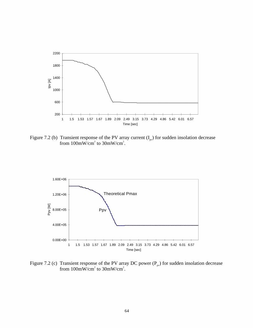
64

200

600

1000

1400

1800

2200

1 1.5 1.53 1.57 1.67 1.89 2.09 2.49 3.15 3.73 4.29 4.86 5.42 6.01 6.57Time [sec]

Ipv

[A]

Figure 7.2 (b) Transient response of the PV array current (Ipv) for sudden insolation decreasefrom 100mW/cm2 to 30mW/cm2.

0.00E+00

4.00E+05

8.00E+05

1.20E+06

1.60E+06

1 1.5 1.53 1.57 1.67 1.89 2.09 2.49 3.15 3.73 4.29 4.86 5.42 6.01 6.57Time [sec]

Ppv

[W]

Theoretical Pmax

Ppv

Figure 7.2 (c) Transient response of the PV array DC power (Ppv) for sudden insolation decreasefrom 100mW/cm2 to 30mW/cm2.

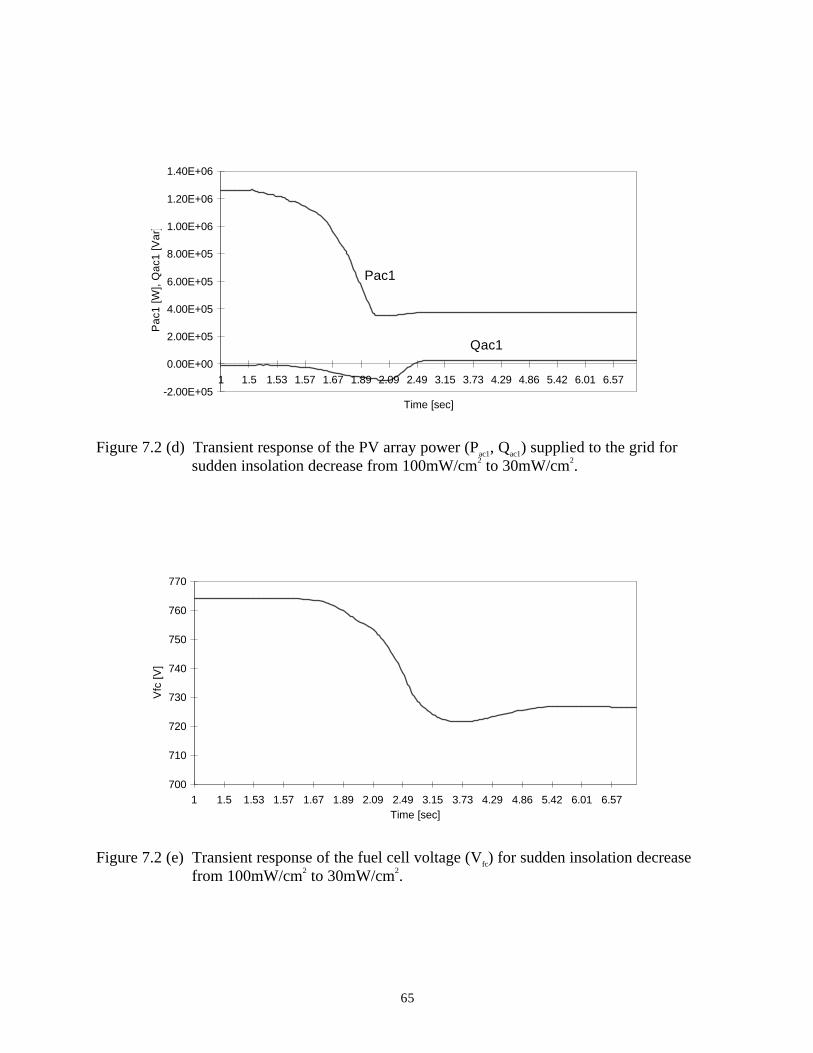
65

-2.00E+05

0.00E+00

2.00E+05

4.00E+05

6.00E+05

8.00E+05

1.00E+06

1.20E+06

1.40E+06

1 1.5 1.53 1.57 1.67 1.89 2.09 2.49 3.15 3.73 4.29 4.86 5.42 6.01 6.57

Time [sec]

Pac

1 [W

], Q

ac1

[Var

]

Pac1

Qac1

Figure 7.2 (d) Transient response of the PV array power (Pac1, Qac1) supplied to the grid forsudden insolation decrease from 100mW/cm2 to 30mW/cm2.

700

710

720

730

740

750

760

770

1 1.5 1.53 1.57 1.67 1.89 2.09 2.49 3.15 3.73 4.29 4.86 5.42 6.01 6.57Time [sec]

Vfc

[V]

Figure 7.2 (e) Transient response of the fuel cell voltage (Vfc) for sudden insolation decreasefrom 100mW/cm2 to 30mW/cm2.

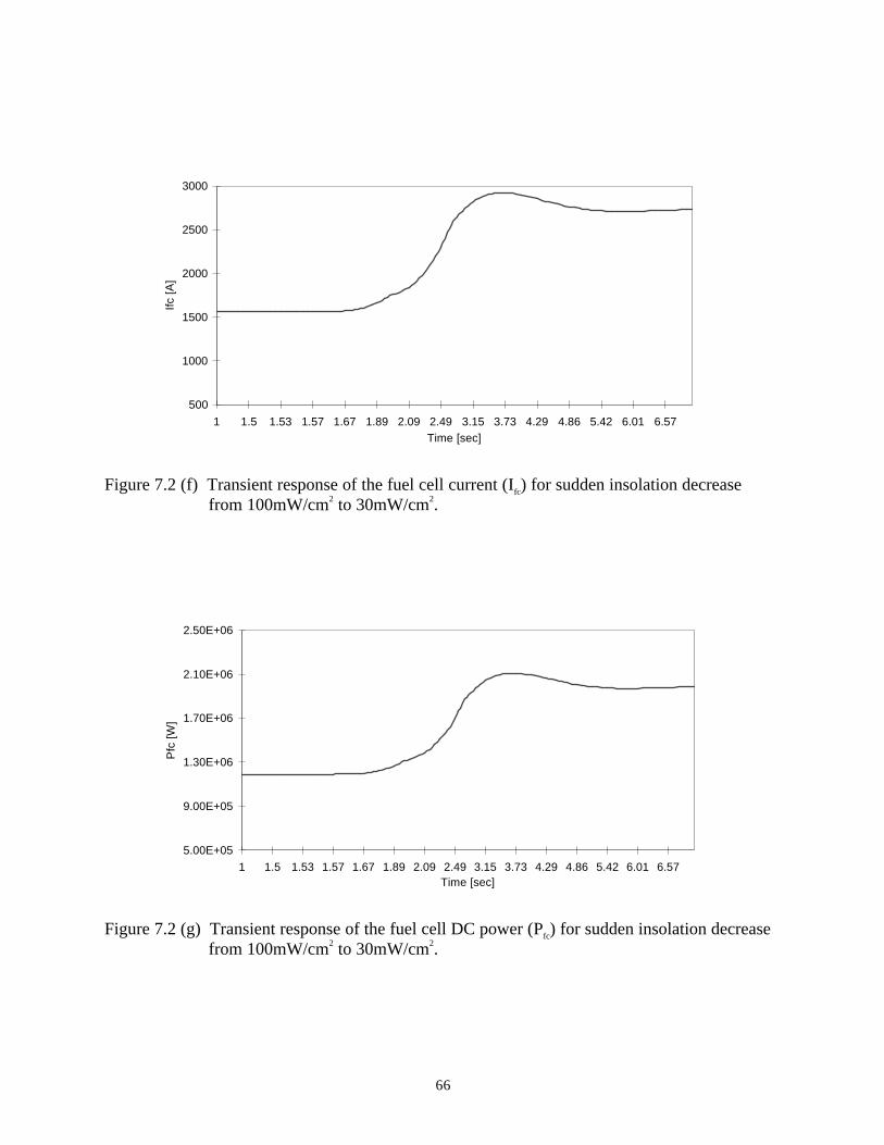
66

500

1000

1500

2000

2500

3000

1 1.5 1.53 1.57 1.67 1.89 2.09 2.49 3.15 3.73 4.29 4.86 5.42 6.01 6.57Time [sec]

Ifc [A

]

Figure 7.2 (f) Transient response of the fuel cell current (Ifc) for sudden insolation decreasefrom 100mW/cm2 to 30mW/cm2.

5.00E+05

9.00E+05

1.30E+06

1.70E+06

2.10E+06

2.50E+06

1 1.5 1.53 1.57 1.67 1.89 2.09 2.49 3.15 3.73 4.29 4.86 5.42 6.01 6.57Time [sec]

Pfc

[W]

Figure 7.2 (g) Transient response of the fuel cell DC power (Pfc) for sudden insolation decreasefrom 100mW/cm2 to 30mW/cm2.

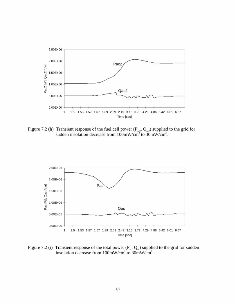
67

0.00E+00

5.00E+05

1.00E+06

1.50E+06

2.00E+06

2.50E+06

1 1.5 1.53 1.57 1.67 1.89 2.09 2.49 3.15 3.73 4.29 4.86 5.42 6.01 6.57Time [sec]

Pac

2 [W

], Q

ac2

[Var

] Pac2

Qac2

Figure 7.2 (h) Transient response of the fuel cell power (Pac2, Qac2) supplied to the grid forsudden insolation decrease from 100mW/cm2 to 30mW/cm2.

0.00E+00

5.00E+05

1.00E+06

1.50E+06

2.00E+06

2.50E+06

1 1.5 1.53 1.57 1.67 1.89 2.09 2.49 3.15 3.73 4.29 4.86 5.42 6.01 6.57Time [sec]

Pac

[W],

Qac

[Var

] Pac

Qac

Figure 7.2 (i) Transient response of the total power (Pac, Qac) supplied to the grid for suddeninsolation decrease from 100mW/cm2 to 30mW/cm2.

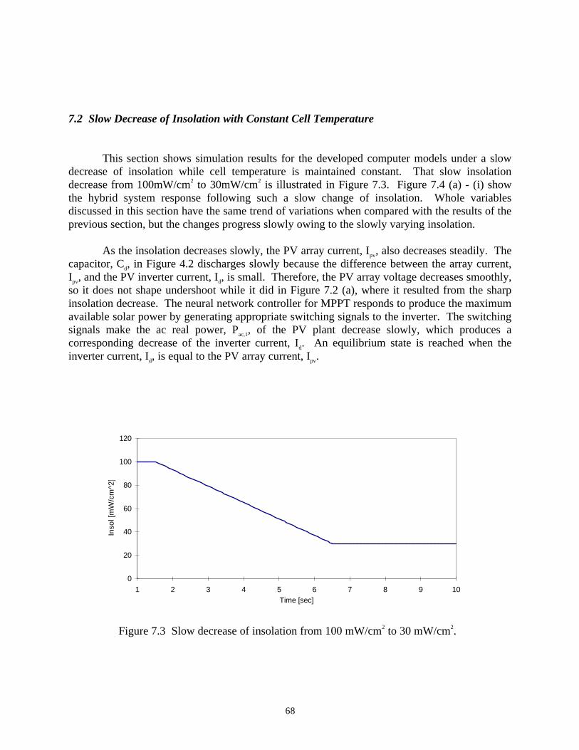
68

7.2 Slow Decrease of Insolation with Constant Cell Temperature

This section shows simulation results for the developed computer models under a slowdecrease of insolation while cell temperature is maintained constant. That slow insolationdecrease from 100mW/cm2 to 30mW/cm2 is illustrated in Figure 7.3. Figure 7.4 (a) - (i) showthe hybrid system response following such a slow change of insolation. Whole variablesdiscussed in this section have the same trend of variations when compared with the results of theprevious section, but the changes progress slowly owing to the slowly varying insolation.

As the insolation decreases slowly, the PV array current, Ipv, also decreases steadily. Thecapacitor, Cd, in Figure 4.2 discharges slowly because the difference between the array current,Ipv, and the PV inverter current, Id, is small. Therefore, the PV array voltage decreases smoothly,so it does not shape undershoot while it did in Figure 7.2 (a), where it resulted from the sharpinsolation decrease. The neural network controller for MPPT responds to produce the maximumavailable solar power by generating appropriate switching signals to the inverter. The switchingsignals make the ac real power, Pac,1, of the PV plant decrease slowly, which produces acorresponding decrease of the inverter current, Id. An equilibrium state is reached when theinverter current, Id, is equal to the PV array current, Ipv.

0

20

40

60

80

100

120

1 2 3 4 5 6 7 8 9 10Time [sec]

Inso

l [m

W/c

m^2

]

Figure 7.3 Slow decrease of insolation from 100 mW/cm2 to 30 mW/cm2.

69

When the insolation decreases slowly, the PV array voltage, Vpv, also decreases asdiscussed above. Since the switching signals from the NN controller can nearly catch up withthe slowly varying insolation, the decrease of the inverter ac voltage is very small. This causesthe PV reactive power supplied to the grid from the PV power plant to decrease a little as shownin Figure 7.4 (d) compared with Figure 7.2 (d). The NN controller operates to bring the reactivepower back to zero, so equilibrium can be achieved.

When the ac real power, Pac,1, of the PV plant decreases as a result of the slow insolationdecrease, the real power error, errP, increases. That error signal goes through the PI compensatorto cause not only the fuel cell current, Ifc, to increase but also the output voltage of the phasecontroller to increase. Then the ac real power, Pac,2, of the fuel cell plant increases slowly tocompensate for the down of the PV power. Since the response time of the fuel cell stacks isshort enough to follow such a slow change of the PV power, the fuel cell voltage does not shapeundershoot and the fuel cell current does not shape overshoot. When the response of Figure 7.4(i) is compared with that of Figure 7.2 (i), the former does not show a sharp variation of the totalreal power because the insolation changes slowly. Therefore, the fuel cell power plant canaccurately compensate for the PV power variations. On the other hand, as the ac reactive power,Qac,1, of the PV plant decreases slowly, the reactive power error, errQ, increases. That error signalcauses the output voltage of the angle controller to decrease so that an increase of the reactivepower of the fuel cell plant can be achieved. Therefore, variations of the total ac reactive power,Qac, from the PV and fuel cell plants are very small and Qac is well-maintained at the reactivepower command, Qcom.

620

640

660

680

700

720

740

1 1.35 1.43 1.51 1.65 1.98 2.7 4.1 4.85 5.6 6.37 7.12 7.89 8.62 9.39Time [sec]

Vpv

[V]

Figure 7.4 (a) Transient response of the PV array voltage (Vpv) for slow insolation decreasefrom 100mW/cm2 to 30mW/cm2.

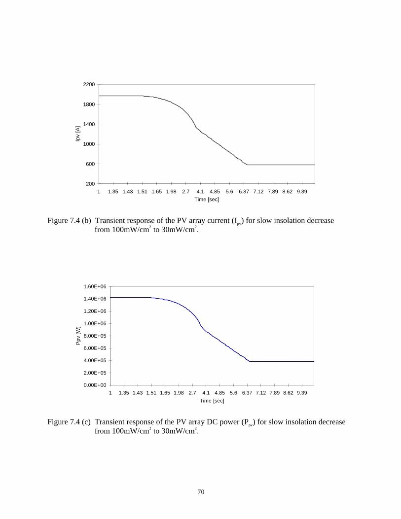
70

200

600

1000

1400

1800

2200

1 1.35 1.43 1.51 1.65 1.98 2.7 4.1 4.85 5.6 6.37 7.12 7.89 8.62 9.39Time [sec]

Ipv

[A]

Figure 7.4 (b) Transient response of the PV array current (Ipv) for slow insolation decreasefrom 100mW/cm2 to 30mW/cm2.

0.00E+00

2.00E+05

4.00E+05

6.00E+05

8.00E+05

1.00E+06

1.20E+06

1.40E+06

1.60E+06

1 1.35 1.43 1.51 1.65 1.98 2.7 4.1 4.85 5.6 6.37 7.12 7.89 8.62 9.39Time [sec]

Ppv

[W]

Figure 7.4 (c) Transient response of the PV array DC power (Ppv) for slow insolation decreasefrom 100mW/cm2 to 30mW/cm2.

71

0.00E+00

2.00E+05

4.00E+05

6.00E+05

8.00E+05

1.00E+06

1.20E+06

1.40E+06

1 1.35 1.43 1.51 1.65 1.98 2.7 4.1 4.85 5.6 6.37 7.12 7.89 8.62 9.39Time [sec]

Pac

1 [W

], Q

ac1

[Var

] Pac1

Qac1

Figure 7.4 (d) Transient response of the PV array power (Pac1, Qac1) supplied to the grid forslow insolation decrease from 100mW/cm2 to 30mW/cm2.

700

710

720

730

740

750

760

770

1 1.35 1.43 1.51 1.65 1.98 2.7 4.1 4.85 5.6 6.37 7.12 7.89 8.62 9.39Time [sec]

Vfc

[V]

Figure 7.4 (e) Transient response of the fuel cell voltage (Vfc) for slow insolation decreasefrom 100mW/cm2 to 30mW/cm2.

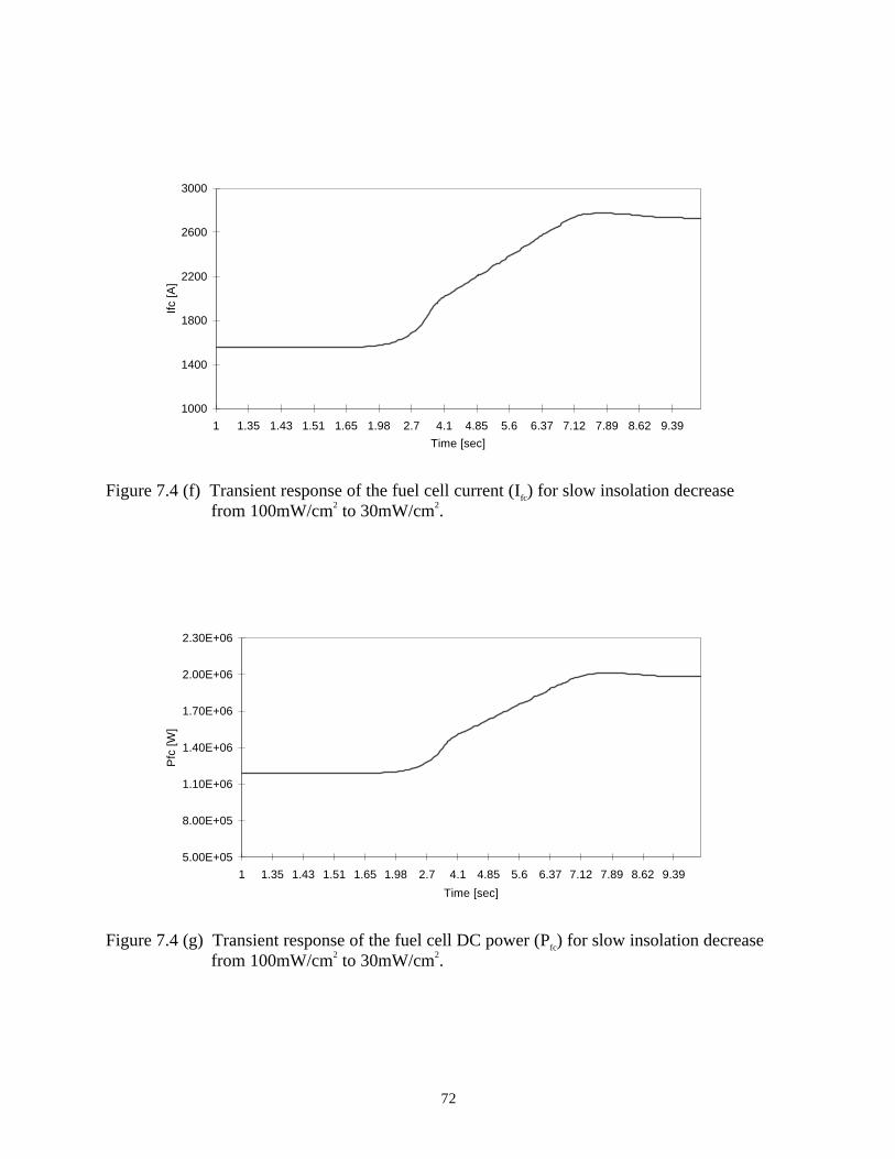
72

1000

1400

1800

2200

2600

3000

1 1.35 1.43 1.51 1.65 1.98 2.7 4.1 4.85 5.6 6.37 7.12 7.89 8.62 9.39Time [sec]

Ifc [A

]

Figure 7.4 (f) Transient response of the fuel cell current (Ifc) for slow insolation decreasefrom 100mW/cm2 to 30mW/cm2.

5.00E+05

8.00E+05

1.10E+06

1.40E+06

1.70E+06

2.00E+06

2.30E+06

1 1.35 1.43 1.51 1.65 1.98 2.7 4.1 4.85 5.6 6.37 7.12 7.89 8.62 9.39

Time [sec]

Pfc

[W]

Figure 7.4 (g) Transient response of the fuel cell DC power (Pfc) for slow insolation decreasefrom 100mW/cm2 to 30mW/cm2.

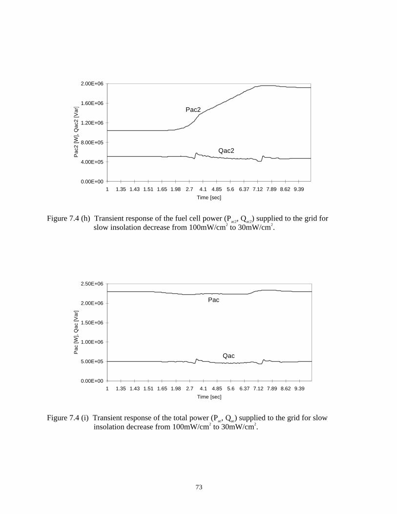
73

0.00E+00

4.00E+05

8.00E+05

1.20E+06

1.60E+06

2.00E+06

1 1.35 1.43 1.51 1.65 1.98 2.7 4.1 4.85 5.6 6.37 7.12 7.89 8.62 9.39Time [sec]

Pac

2 [W

], Q

ac2

[Var

] Pac2

Qac2

Figure 7.4 (h) Transient response of the fuel cell power (Pac2, Qac2) supplied to the grid forslow insolation decrease from 100mW/cm2 to 30mW/cm2.

0.00E+00

5.00E+05

1.00E+06

1.50E+06

2.00E+06

2.50E+06

1 1.35 1.43 1.51 1.65 1.98 2.7 4.1 4.85 5.6 6.37 7.12 7.89 8.62 9.39

Time [sec]

Pac

[W],

Qac

[Var

]

Pac

Qac

Figure 7.4 (i) Transient response of the total power (Pac, Qac) supplied to the grid for slowinsolation decrease from 100mW/cm2 to 30mW/cm2.

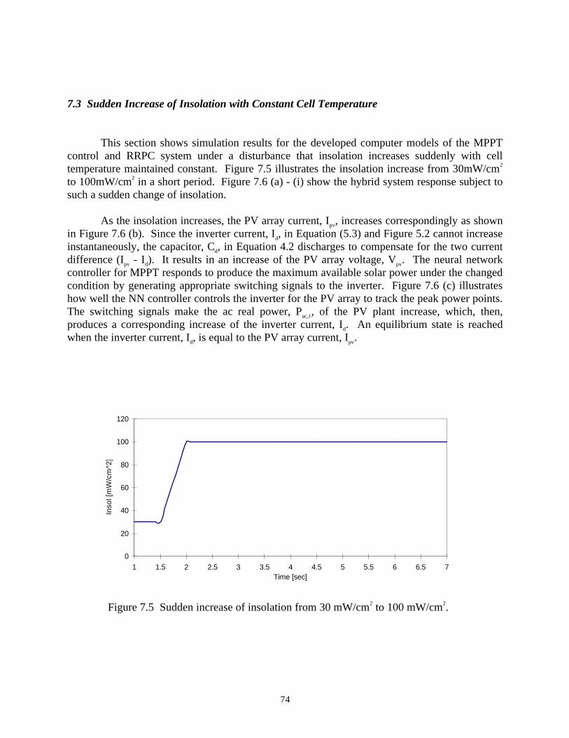
74

7.3 Sudden Increase of Insolation with Constant Cell Temperature

This section shows simulation results for the developed computer models of the MPPTcontrol and RRPC system under a disturbance that insolation increases suddenly with celltemperature maintained constant. Figure 7.5 illustrates the insolation increase from 30mW/cm2

to 100mW/cm2 in a short period. Figure 7.6 (a) - (i) show the hybrid system response subject tosuch a sudden change of insolation.

As the insolation increases, the PV array current, Ipv, increases correspondingly as shownin Figure 7.6 (b). Since the inverter current, Id, in Equation (5.3) and Figure 5.2 cannot increaseinstantaneously, the capacitor, Cd, in Equation 4.2 discharges to compensate for the two currentdifference (Ipv - Id). It results in an increase of the PV array voltage, Vpv. The neural networkcontroller for MPPT responds to produce the maximum available solar power under the changedcondition by generating appropriate switching signals to the inverter. Figure 7.6 (c) illustrateshow well the NN controller controls the inverter for the PV array to track the peak power points.The switching signals make the ac real power, Pac,1, of the PV plant increase, which, then,produces a corresponding increase of the inverter current, Id. An equilibrium state is reachedwhen the inverter current, Id, is equal to the PV array current, Ipv.

0

20

40

60

80

100

120

1 1.5 2 2.5 3 3.5 4 4.5 5 5.5 6 6.5 7Time [sec]

Inso

l [m

W/c

m^2

]

Figure 7.5 Sudden increase of insolation from 30 mW/cm2 to 100 mW/cm2.

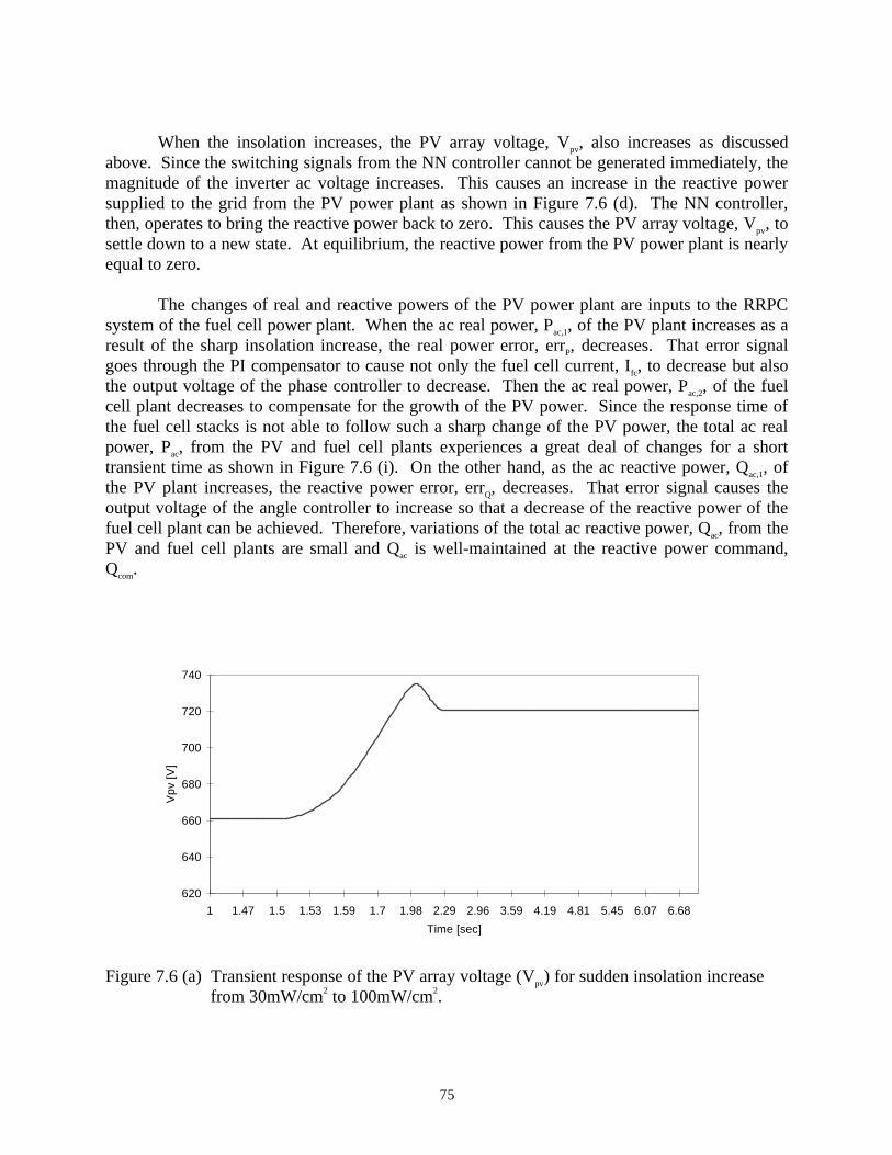
75

When the insolation increases, the PV array voltage, Vpv, also increases as discussedabove. Since the switching signals from the NN controller cannot be generated immediately, themagnitude of the inverter ac voltage increases. This causes an increase in the reactive powersupplied to the grid from the PV power plant as shown in Figure 7.6 (d). The NN controller,then, operates to bring the reactive power back to zero. This causes the PV array voltage, Vpv, tosettle down to a new state. At equilibrium, the reactive power from the PV power plant is nearlyequal to zero.

The changes of real and reactive powers of the PV power plant are inputs to the RRPCsystem of the fuel cell power plant. When the ac real power, Pac,1, of the PV plant increases as aresult of the sharp insolation increase, the real power error, errP, decreases. That error signalgoes through the PI compensator to cause not only the fuel cell current, Ifc, to decrease but alsothe output voltage of the phase controller to decrease. Then the ac real power, Pac,2, of the fuelcell plant decreases to compensate for the growth of the PV power. Since the response time ofthe fuel cell stacks is not able to follow such a sharp change of the PV power, the total ac realpower, Pac, from the PV and fuel cell plants experiences a great deal of changes for a shorttransient time as shown in Figure 7.6 (i). On the other hand, as the ac reactive power, Qac,1, ofthe PV plant increases, the reactive power error, errQ, decreases. That error signal causes theoutput voltage of the angle controller to increase so that a decrease of the reactive power of thefuel cell plant can be achieved. Therefore, variations of the total ac reactive power, Qac, from thePV and fuel cell plants are small and Qac is well-maintained at the reactive power command,Qcom.

620

640

660

680

700

720

740

1 1.47 1.5 1.53 1.59 1.7 1.98 2.29 2.96 3.59 4.19 4.81 5.45 6.07 6.68

Time [sec]

Vpv

[V]

Figure 7.6 (a) Transient response of the PV array voltage (Vpv) for sudden insolation increasefrom 30mW/cm2 to 100mW/cm2.

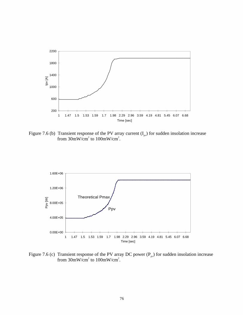
76

200

600

1000

1400

1800

2200

1 1.47 1.5 1.53 1.59 1.7 1.98 2.29 2.96 3.59 4.19 4.81 5.45 6.07 6.68

Time [sec]

Ipv

[A]

Figure 7.6 (b) Transient response of the PV array current (Ipv) for sudden insolation increasefrom 30mW/cm2 to 100mW/cm2.

0.00E+00

4.00E+05

8.00E+05

1.20E+06

1.60E+06

1 1.47 1.5 1.53 1.59 1.7 1.98 2.29 2.96 3.59 4.19 4.81 5.45 6.07 6.68Time [sec]

Ppv

[W] Theoretical Pmax

Ppv

Figure 7.6 (c) Transient response of the PV array DC power (Ppv) for sudden insolation increasefrom 30mW/cm2 to 100mW/cm2.

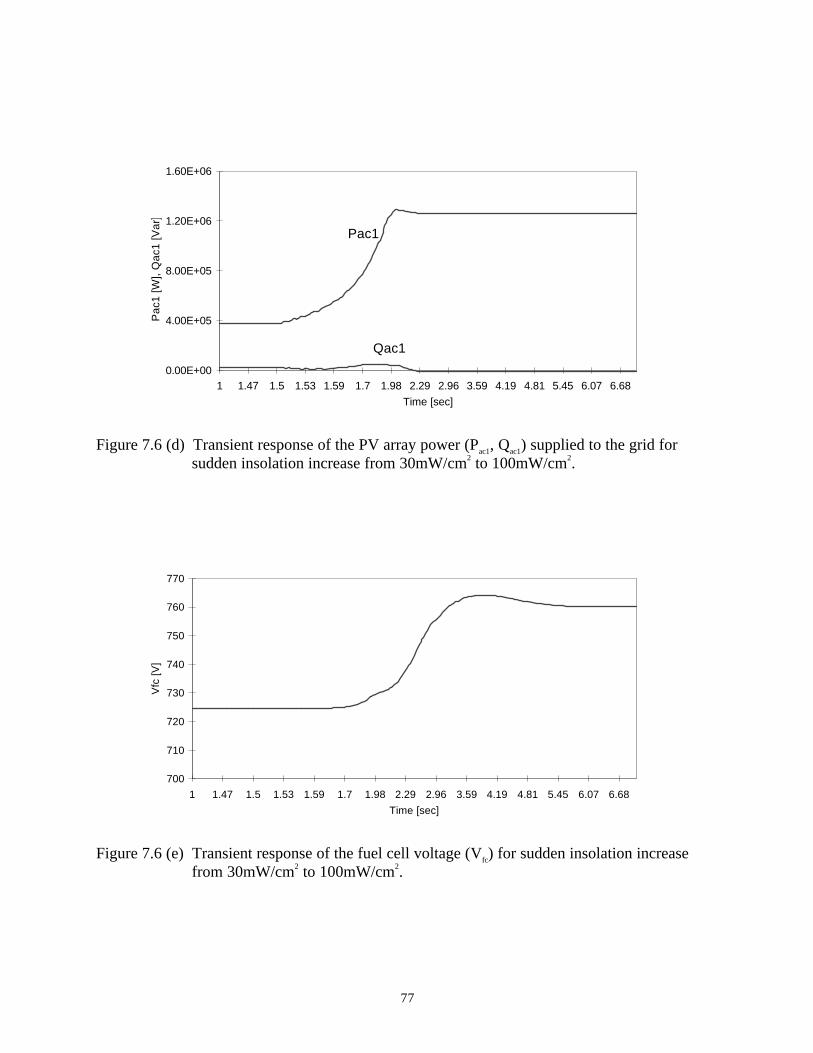
77

0.00E+00

4.00E+05

8.00E+05

1.20E+06

1.60E+06

1 1.47 1.5 1.53 1.59 1.7 1.98 2.29 2.96 3.59 4.19 4.81 5.45 6.07 6.68Time [sec]

Pac

1 [W

], Q

ac1

[Var

]

Pac1

Qac1

Figure 7.6 (d) Transient response of the PV array power (Pac1, Qac1) supplied to the grid forsudden insolation increase from 30mW/cm2 to 100mW/cm2.

700

710

720

730

740

750

760

770

1 1.47 1.5 1.53 1.59 1.7 1.98 2.29 2.96 3.59 4.19 4.81 5.45 6.07 6.68Time [sec]

Vfc

[V]

Figure 7.6 (e) Transient response of the fuel cell voltage (Vfc) for sudden insolation increasefrom 30mW/cm2 to 100mW/cm2.

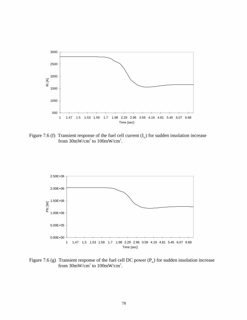
78

500

1000

1500

2000

2500

3000

1 1.47 1.5 1.53 1.59 1.7 1.98 2.29 2.96 3.59 4.19 4.81 5.45 6.07 6.68Time [sec]

Ifc [A

]

Figure 7.6 (f) Transient response of the fuel cell current (Ifc) for sudden insolation increasefrom 30mW/cm2 to 100mW/cm2.

0.00E+00

5.00E+05

1.00E+06

1.50E+06

2.00E+06

2.50E+06

1 1.47 1.5 1.53 1.59 1.7 1.98 2.29 2.96 3.59 4.19 4.81 5.45 6.07 6.68Time [sec]

Pfc

[W]

Figure 7.6 (g) Transient response of the fuel cell DC power (Pfc) for sudden insolation increasefrom 30mW/cm2 to 100mW/cm2.

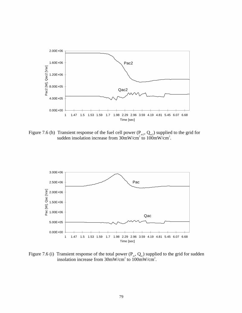
79

0.00E+00

4.00E+05

8.00E+05

1.20E+06

1.60E+06

2.00E+06

1 1.47 1.5 1.53 1.59 1.7 1.98 2.29 2.96 3.59 4.19 4.81 5.45 6.07 6.68Time [sec]

Pac

2 [W

], Q

ac2

[Var

] Pac2

Qac2

Figure 7.6 (h) Transient response of the fuel cell power (Pac2, Qac2) supplied to the grid forsudden insolation increase from 30mW/cm2 to 100mW/cm2.

0.00E+00

5.00E+05

1.00E+06

1.50E+06

2.00E+06

2.50E+06

3.00E+06

1 1.47 1.5 1.53 1.59 1.7 1.98 2.29 2.96 3.59 4.19 4.81 5.45 6.07 6.68Time [sec]

Pac

[W],

Qac

[Var

]

Pac

Qac

Figure 7.6 (i) Transient response of the total power (Pac, Qac) supplied to the grid for suddeninsolation increase from 30mW/cm2 to 100mW/cm2.

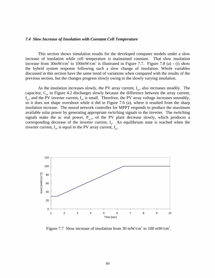
80

7.4 Slow Increase of Insolation with Constant Cell Temperature

This section shows simulation results for the developed computer models under a slowincrease of insolation while cell temperature is maintained constant. That slow insolationincrease from 30mW/cm2 to 100mW/cm2 is illustrated in Figure 7.7. Figure 7.8 (a) - (i) showthe hybrid system response following such a slow change of insolation. Whole variablesdiscussed in this section have the same trend of variations when compared with the results of theprevious section, but the changes progress slowly owing to the slowly varying insolation.

As the insolation increases slowly, the PV array current, Ipv, also increases steadily. Thecapacitor, Cd, in Figure 4.2 discharges slowly because the difference between the array current,Ipv, and the PV inverter current, Id, is small. Therefore, the PV array voltage increases smoothly,so it does not shape overshoot while it did in Figure 7.6 (a), where it resulted from the sharpinsolation increase. The neural network controller for MPPT responds to produce the maximumavailable solar power by generating appropriate switching signals to the inverter. The switchingsignals make the ac real power, Pac,1, of the PV plant decrease slowly, which produces acorresponding decrease of the inverter current, Id. An equilibrium state is reached when theinverter current, Id, is equal to the PV array current, Ipv.

0

20

40

60

80

100

120

1 2 3 4 5 6 7 8 9 10Time [sec]

Inso

l [m

W/c

m^2

]

Figure 7.7 Slow increase of insolation from 30 mW/cm2 to 100 mW/cm2.

81

When the insolation increases slowly, the PV array voltage, Vpv, also increases asdiscussed above. Since the switching signals from the NN controller can nearly catch up withthe slowly varying insolation, the increase of the inverter ac voltage is very small. This causesthe PV reactive power supplied to the grid from the PV power plant to increase a little as shownin Figure 7.8 (d) compared with Figure 7.6 (d). The NN controller operates to bring the reactivepower back to zero, so equilibrium can be achieved.

When the ac real power, Pac,1, of the PV plant increases as a result of the slow insolationincrease, the real power error, errP, decreases. That error signal goes through the PI compensatorto cause not only the fuel cell current, Ifc, to decrease but also the output voltage of the phasecontroller to decrease. Then the ac real power, Pac,2, of the fuel cell plant decreases slowly tocompensate for the growth of the PV power. Since the response time of the fuel cell stacks isshort enough to follow such a slow change of the PV power, the fuel cell voltage does not shapeovershoot and the fuel cell current does not shape undershoot. When the response of Figure 7.8(i) is compared with that of Figure 7.6 (i), the former does not show a sharp variation of the totalreal power because the insolation changes slowly. Therefore, the fuel cell power plant canaccurately compensate for the PV power variations. On the other hand, as the ac reactive power,Qac,1, of the PV plant increases slowly, the reactive power error, errQ, decreases. That error signalcauses the output voltage of the angle controller to increase so that a decrease of the reactivepower of the fuel cell plant can be achieved. Therefore, variations of the total ac reactive power,Qac, from the PV and fuel cell plants are very small and Qac is well-maintained at the reactivepower command, Qcom.

620

640

660

680

700

720

740

1 1.52 1.65 1.98 2.72 3.84 4.57 5.29 6.01 6.64 7.43 8.13 8.83 9.53Time [sec]

Vpv

[V]

Figure 7.8 (a) Transient response of the PV array voltage (Vpv) for slow insolation increasefrom 30mW/cm2 to 100mW/cm2.

82

300

500

700

900

1100

1300

1500

1700

1900

2100

1 1.52 1.65 1.98 2.72 3.84 4.57 5.29 6.01 6.64 7.43 8.13 8.83 9.53Time [sec]

Ipv

[A]

Figure 7.8 (b) Transient response of the PV array current (Ipv) for slow insolation increasefrom 30mW/cm2 to 100mW/cm2.

0.00E+00

4.00E+05

8.00E+05

1.20E+06

1.60E+06

1 1.52 1.65 1.98 2.72 3.84 4.57 5.29 6.01 6.64 7.43 8.13 8.83 9.53Time [sec]

Ppv

[W]

Figure 7.8 (c) Transient response of the PV array DC power (Ppv) for slow insolation increasefrom 30mW/cm2 to 100mW/cm2.

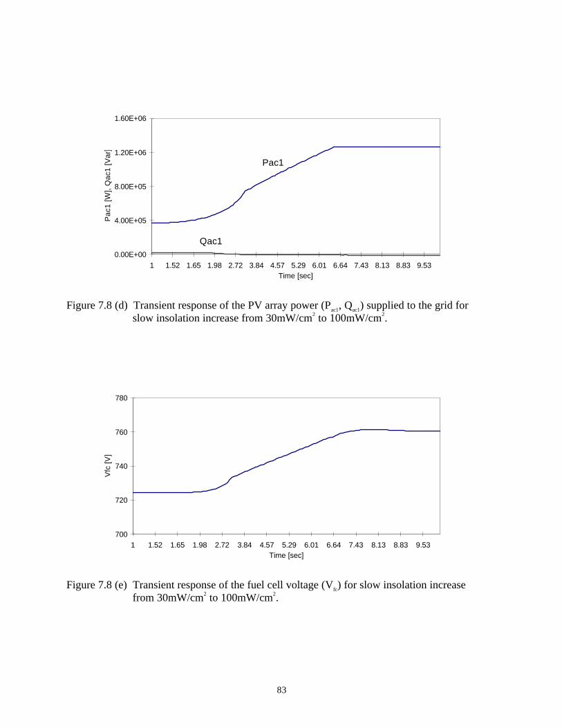
83

0.00E+00

4.00E+05

8.00E+05

1.20E+06

1.60E+06

1 1.52 1.65 1.98 2.72 3.84 4.57 5.29 6.01 6.64 7.43 8.13 8.83 9.53Time [sec]

Pac

1 [W

], Q

ac1

[Var

]

Pac1

Qac1

Figure 7.8 (d) Transient response of the PV array power (Pac1, Qac1) supplied to the grid forslow insolation increase from 30mW/cm2 to 100mW/cm2.

700

720

740

760

780

1 1.52 1.65 1.98 2.72 3.84 4.57 5.29 6.01 6.64 7.43 8.13 8.83 9.53Time [sec]

Vfc

[V]

Figure 7.8 (e) Transient response of the fuel cell voltage (Vfc) for slow insolation increasefrom 30mW/cm2 to 100mW/cm2.

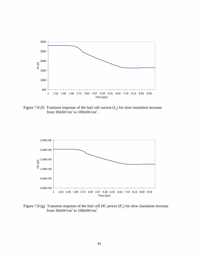
84

500

1000

1500

2000

2500

3000

1 1.52 1.65 1.98 2.72 3.84 4.57 5.29 6.01 6.64 7.43 8.13 8.83 9.53Time [sec]

Ifc [A

]

Figure 7.8 (f) Transient response of the fuel cell current (Ifc) for slow insolation increasefrom 30mW/cm2 to 100mW/cm2.

0.00E+00

5.00E+05

1.00E+06

1.50E+06

2.00E+06

2.50E+06

1 1.52 1.65 1.98 2.72 3.84 4.57 5.29 6.01 6.64 7.43 8.13 8.83 9.53Time [sec]

Pfc

[W]

Figure 7.8 (g) Transient response of the fuel cell DC power (Pfc) for slow insolation increasefrom 30mW/cm2 to 100mW/cm2.

85

0.00E+00

4.00E+05

8.00E+05

1.20E+06

1.60E+06

2.00E+06

1 1.52 1.65 1.98 2.72 3.84 4.57 5.29 6.01 6.64 7.43 8.13 8.83 9.53Time [sec]

Pac

2 [W

], Q

ac2

[Var

] Pac2

Qac2

Figure 7.8 (h) Transient response of the fuel cell power (Pac2, Qac2) supplied to the grid forslow insolation increase from 30mW/cm2 to 100mW/cm2.

0.00E+00

5.00E+05

1.00E+06

1.50E+06

2.00E+06

2.50E+06

1 1.52 1.65 1.98 2.72 3.84 4.57 5.29 6.01 6.64 7.43 8.13 8.83 9.53Time [sec]

Pac

[W],

Qac

[Var

]

Pac

Qac

Figure 7.8 (i) Transient response of the total power (Pac, Qac) supplied to the grid for slowinsolation increase from 30mW/cm2 to 100mW/cm2.

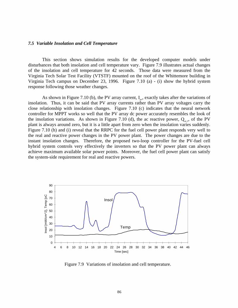
86

7.5 Variable Insolation and Cell Temperature

This section shows simulation results for the developed computer models underdisturbances that both insolation and cell temperature vary. Figure 7.9 illustrates actual changesof the insolation and cell temperature for 42 seconds. Those data were measured from theVirginia Tech Solar Test Facility (VTSTF) mounted on the roof of the Whittemore building inVirginia Tech campus on December 23, 1996. Figure 7.10 (a) - (i) show the hybrid systemresponse following those weather changes.

As shown in Figure 7.10 (b), the PV array current, Ipv, exactly takes after the variations ofinsolation. Thus, it can be said that PV array currents rather than PV array voltages carry theclose relationship with insolation changes. Figure 7.10 (c) indicates that the neural networkcontroller for MPPT works so well that the PV array dc power accurately resembles the look ofthe insolation variations. As shown in Figure 7.10 (d), the ac reactive power, Qac,1, of the PVplant is always around zero, but it is a little apart from zero when the insolation varies suddenly.Figure 7.10 (h) and (i) reveal that the RRPC for the fuel cell power plant responds very well tothe real and reactive power changes in the PV power plant. The power changes are due to theinstant insolation changes. Therefore, the proposed two-loop controller for the PV-fuel cellhybrid system controls very effectively the inverters so that the PV power plant can alwaysachieve maximum available solar power points. Moreover, the fuel cell power plant can satisfythe system-side requirement for real and reactive powers.

0

10

20

30

40

50

60

70

80

90

4 6 8 10 12 14 16 18 20 22 24 26 28 30 32 34 36 38 40 42 44 46Time [sec]

Inso

l [m

W/c

m^2

], T

emp

[oC

]

Insol

Temp

Figure 7.9 Variations of insolation and cell temperature.

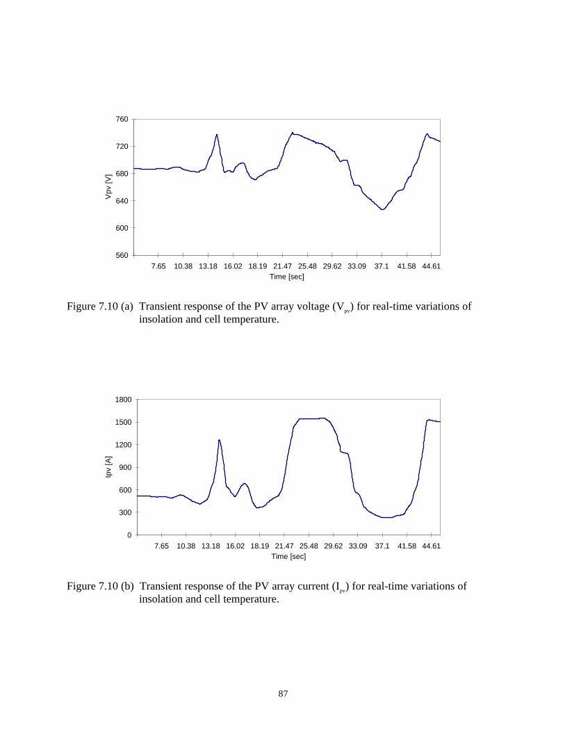
87

560

600

640

680

720

760

7.65 10.38 13.18 16.02 18.19 21.47 25.48 29.62 33.09 37.1 41.58 44.61Time [sec]

Vpv

[V]

Figure 7.10 (a) Transient response of the PV array voltage (Vpv) for real-time variations of insolation and cell temperature.

0

300

600

900

1200

1500

1800

7.65 10.38 13.18 16.02 18.19 21.47 25.48 29.62 33.09 37.1 41.58 44.61Time [sec]

Ipv

[A]

Figure 7.10 (b) Transient response of the PV array current (Ipv) for real-time variations of insolation and cell temperature.

88

0.00E+00

3.00E+05

6.00E+05

9.00E+05

1.20E+06

1.50E+06

7.65 10.38 13.18 16.02 18.19 21.47 25.48 29.62 33.09 37.1 41.58 44.61Time [sec]

Ppv

[W]

Figure 7.10 (c) Transient response of the PV array DC power (Ppv) for real-time variations of insolation and cell temperature.

-2.00E+05

0.00E+00

2.00E+05

4.00E+05

6.00E+05

8.00E+05

1.00E+06

1.20E+06

7.65 10.38 13.18 16.02 18.19 21.47 25.48 29.62 33.09 37.1 41.58 44.61

Time [sec]

Pac

1 [W

], Q

ac1

[Var

] Pac1

Qac1

Figure 7.10 (d) Transient response of the PV array power (Pac1,Qac1) supplied to the grid for real- time variations of insolation and cell temperature.

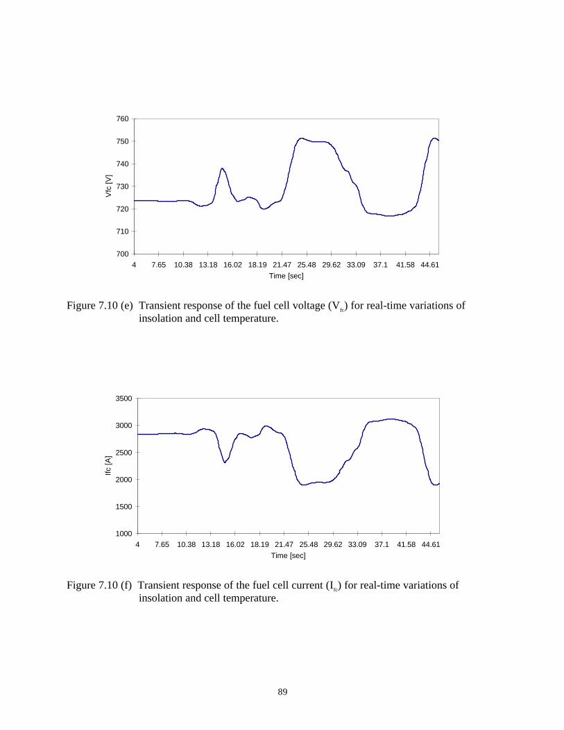
89

700

710

720

730

740

750

760

4 7.65 10.38 13.18 16.02 18.19 21.47 25.48 29.62 33.09 37.1 41.58 44.61Time [sec]

Vfc

[V]

Figure 7.10 (e) Transient response of the fuel cell voltage (Vfc) for real-time variations of insolation and cell temperature.

1000

1500

2000

2500

3000

3500

4 7.65 10.38 13.18 16.02 18.19 21.47 25.48 29.62 33.09 37.1 41.58 44.61Time [sec]

Ifc [A

]

Figure 7.10 (f) Transient response of the fuel cell current (Ifc) for real-time variations of insolation and cell temperature.

90

5.00E+05

1.00E+06

1.50E+06

2.00E+06

2.50E+06

4 7.65 10.38 13.18 16.02 18.19 21.47 25.48 29.62 33.09 37.1 41.58 44.61Time [sec]

Pfc

[W]

Figure 7.10 (g) Transient response of the fuel cell DC power (Pfc) for real-time variations of insolation and cell temperature.

0.00E+00

5.00E+05

1.00E+06

1.50E+06

2.00E+06

2.50E+06

4 7.65 10.38 13.18 16.02 18.19 21.47 25.48 29.62 33.09 37.1 41.58 44.61Time [sec]

Pac

2 [W

], Q

ac2

[Var

] Pac2

Qac2

Figure 7.10 (h) Transient response of the fuel cell power (Pac2, Qac2) supplied to the grid for real- time variations of insolation and cell temperature.

91

0.00E+00

5.00E+05

1.00E+06

1.50E+06

2.00E+06

2.50E+06

3.00E+06

4 7.65 10.38 13.18 16.02 18.19 21.47 25.48 29.62 33.09 37.1 41.58 44.61Time [sec]

Pac

[W],

Qac

[Var

]

Pac

Qac

Figure 7.10 (i) Transient response of the total power (Pac, Qac) supplied to the grid for real-time variations of insolation and cell temperature.

7.6 Change of Power Commands with Variable Insolation and Cell Temperature

This section shows simulation results for the developed computer models of the MPPTcontrol and RRPC system under the same weather condition as in the previous section but with achange of power commands in the middle of time period. The real and reactive powercommands are changed from 2.3MW, 0.5MVar to 1.5MW, 1.0MVar respectively at the instantof 20 second in time period. Figure 7.11 (a) - (i) show the hybrid system response following thechanges of power commands.

As shown in Figure 7.11 (a), (b), (c) and (d), the variables belonging to the PV powerplant such as Vpv, Ipv, Ppv, Pac,1 and Qac,1 show exactly the same shapes as those in the previoussection. It implies that a change of power commands in the middle of operation does notinfluence the operation of the PV power plant. Instead, the change of power commands is takencharge on by the fuel cell plant. The RRPC for the fuel cell power plant responds so well to thepower command changes that the total real and reactive powers, Pac and Qac, supplied to theutility grid show nice transitions to the new power commands, as shown in Figure 7.11 (i).

92

580

620

660

700

740

780

4 7.16 10 12.37 14.65 17.05 19.63 21.18 24.56 27.89 31.23 34.55 37.96 41.41 44.73Time [sec]

Vpv

[V]

Figure 7.11 (a) Transient response of the PV array voltage (Vpv) for change of power commands with variable insolation and cell temperature.

0

400

800

1200

1600

4 7.16 10 12.37 14.65 17.05 19.63 21.18 24.56 27.89 31.23 34.55 37.96 41.41 44.73Time [sec]

Ipv

[A]

Figure 7.11 (b) Transient response of the PV array current (Ipv) for change of power commands with variable insolation and cell temperature.

93

0.00E+00

3.00E+05

6.00E+05

9.00E+05

1.20E+06

4 7.16 10 12.4 14.7 17.1 19.6 21.2 24.6 27.9 31.2 34.6 38 41.4 44.7Time [sec]

Ppv

[W]

Figure 7.11 (c) Transient response of the PV array power (Ppv) for change of power commands with variable insolation and cell temperature.

-2.00E+05

2.00E+05

6.00E+05

1.00E+06

1.40E+06

4 7.16 10 12.4 14.7 17.1 19.6 21.2 24.6 27.9 31.2 34.6 38 41.4 44.7

Time [sec]

Pac

1 [W

], Q

ac1

[Var

] Pac1

Qac1

Figure 7.11 (d) Transient response of the PV array power (Pac1, Qac1) supplied to the grid for change of power commands with variable insolation and cell temperature.

94

680

720

760

800

840

4 7.16 10 12.37 14.65 17.05 19.63 21.18 24.56 27.89 31.23 34.55 37.96 41.41 44.73Time [sec]

Vfc

[V]

Figure 7.11 (e) Transient response of the fuel cell voltage (Vfc) for change of power commands with variable insolation and cell temperature.

0

500

1000

1500

2000

2500

3000

4 7.16 10 12.37 14.65 17.05 19.63 21.18 24.56 27.89 31.23 34.55 37.96 41.41 44.73Time [sec]

Ifc [A

]

Figure 7.11 (f) Transient response of the fuel cell current (Ifc) for change of power commands with variable insolation and cell temperature.

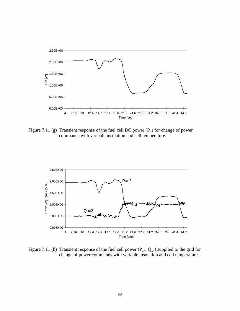
95

0.00E+00

5.00E+05

1.00E+06

1.50E+06

2.00E+06

2.50E+06

4 7.16 10 12.4 14.7 17.1 19.6 21.2 24.6 27.9 31.2 34.6 38 41.4 44.7Time [sec]

Pfc

[W]

Figure 7.11 (g) Transient response of the fuel cell DC power (Pfc) for change of power commands with variable insolation and cell temperature.

0.00E+00

5.00E+05

1.00E+06

1.50E+06

2.00E+06

2.50E+06

4 7.16 10 12.4 14.7 17.1 19.6 21.2 24.6 27.9 31.2 34.6 38 41.4 44.7Time [sec]

Pac

2 [W

], Q

ac2

[Var

] Pac2

Qac2

Figure 7.11 (h) Transient response of the fuel cell power (Pac2, Qac2) supplied to the grid for change of power commands with variable insolation and cell temperature.

96

0.00E+00

5.00E+05

1.00E+06

1.50E+06

2.00E+06

2.50E+06

3.00E+06

4 7.16 10 12.4 14.7 17.1 19.6 21.2 24.6 27.9 31.2 34.6 38 41.4 44.7Time [sec]

Pac

[W],

Qac

[Var

] Pac

Qac

Figure 7.11 (i) Transient response of the total power (Pac, Qac) supplied to the grid for change of power commands with variable insolation and cell temperature.

97

CHAPTER 8

ENVIRONMENTAL EVALUATION

8.1 Introduction

Solar photovoltaic and fuel cell power generations are not free from environmentalimpacts. One major disadvantage of PV power plants is that they require an extensive land forlarge-scale centralized power plant construction. Their indirect impacts on environment duringproduction and disposal of the PV systems cannot be ignored since these materials contain sometoxic elements. Fuel cell systems produce very little amounts of SO2, NOx and other particulatesin the fuel reforming process and their low CO2 emissions result from high energy conversionefficiency.

As two major criteria for calculating environmental impacts of the proposed PV-fuel cellhybrid system, land requirement for the power plant and its lifetime CO2 emissions areconsidered. A requirement of land area would nearly soon be a crucial factor for power stationconstruction in densely populated regions, particularly such as eastern U.S.A, Europe and EastAsia. The world’s rising concern about the increasing CO2 concentration in the atmosphere andits potential impact on global warming gives a suggestion that CO2 emission rates be consideredin selecting electricity generating technologies.

Land area requirement and lifetime CO2 emissions for PV, fuel cell, and conventionalfossil fuel power plants are studied in the first and second part of this chapter, respectively. Thenext part deals with environmental evaluation of the proposed hybrid system. It is carried out interms of land requirement for the plant construction and their lifetime CO2 emissions.

8.2 Land Requirement

98

The land area required for each electric power plant varies over a significant range,depending upon factors such as individual utility design specifications, land costs, and theinstalled capacity. Photovoltaic modules that provide power for remote systems are useful withsmall land disturbance, but, when used for a grid-connected central power station, landrequirement is a major consideration. A PV power plant requires the most extensive land due tothe low energy density of solar radiation and low efficiencies of solar cells. It ranges from20,000 to 35,000 m2 /MW [16].

The amount of land needed for the installation of a fuel cell power plant may berelatively small like 500 - 1,000 m2 /MW owing to the capability of its modular construction[19]. This feature, together with very low environmental impact, may allow fuel cell powerplants to be located close to the point of use, where its waste heat can be used in cogenerationapplications. This siting flexibility of the fuel cell power plants may not only permit a reductionin transmission and distribution loss but also provide for power control close to the load center.Therefore, it is able to make a utility defer transmission and distribution investments.

Table 8.1 summarizes the standard figures of land use for electricity generating powerplants, including conventional fossil-fuel power sources [82]. For coal plants, land area required

Table 8.1 Land requirement for electric power plants.

Power sourcesLand use

[ m2/MW ]

Photovoltaics

Fuel cells

Coal

Oil

Natural gas

20,000

700

3,700*

900

800

* Includes land needed for solid waste disposal.

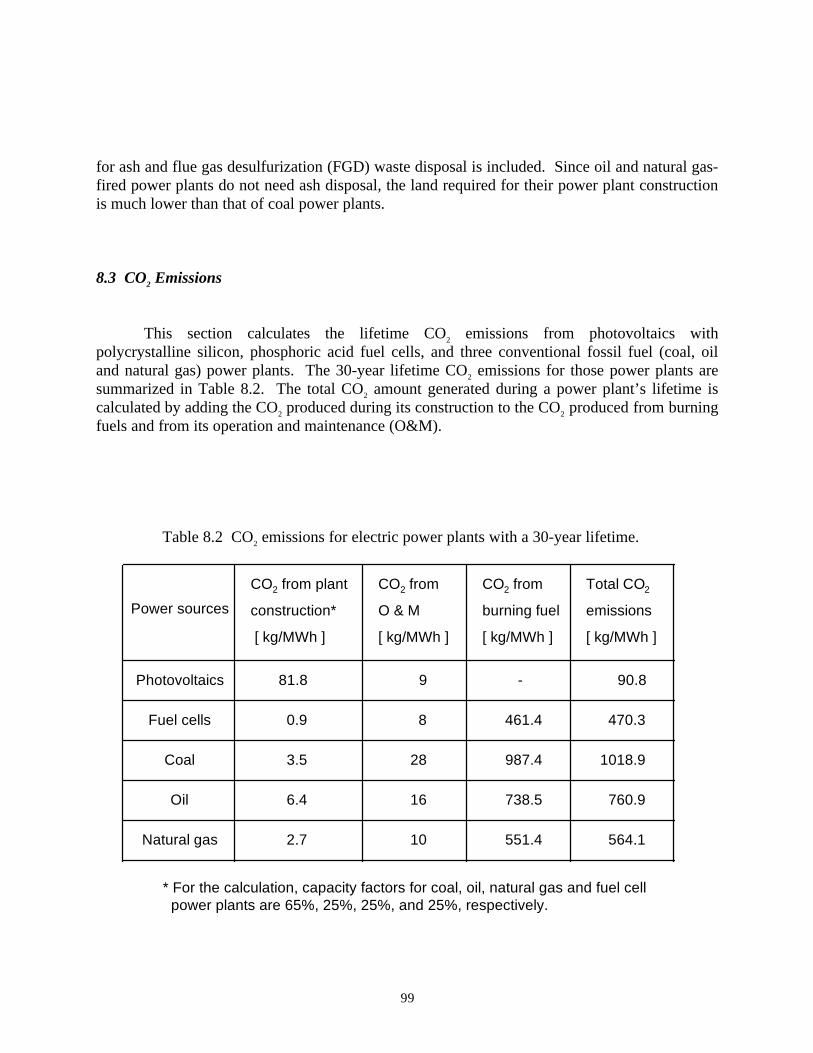
99

for ash and flue gas desulfurization (FGD) waste disposal is included. Since oil and natural gas-fired power plants do not need ash disposal, the land required for their power plant constructionis much lower than that of coal power plants.

8.3 CO2 Emissions

This section calculates the lifetime CO2 emissions from photovoltaics withpolycrystalline silicon, phosphoric acid fuel cells, and three conventional fossil fuel (coal, oiland natural gas) power plants. The 30-year lifetime CO2 emissions for those power plants aresummarized in Table 8.2. The total CO2 amount generated during a power plant’s lifetime iscalculated by adding the CO2 produced during its construction to the CO2 produced from burningfuels and from its operation and maintenance (O&M).

Table 8.2 CO2 emissions for electric power plants with a 30-year lifetime.

Power sources

CO2 from plant

construction*

[ kg/MWh ]

CO2 from

O & M

[ kg/MWh ]

CO2 from

burning fuel

[ kg/MWh ]

Total CO2

emissions

[ kg/MWh ]

Photovoltaics

Fuel cells

Coal

Oil

Natural gas

81.8 9 - 90.8

0.9 8 461.4 470.3

3.5 28 987.4 1018.9

6.4 16 738.5 760.9

2.7 10 551.4 564.1

* For the calculation, capacity factors for coal, oil, natural gas and fuel cell power plants are 65%, 25%, 25%, and 25%, respectively.

100

More than 95% of CO2 produced from fossil fuel-burning power plants is generatedduring their operation as a consequence of fuel combustion. The CO2 productions from coal, oil,and natural gas power plants by burning the fuels are calculated in Appendix A in detail. Thosecalculations are made by using carbon content and heating values for each of the fossil fuels, andelectricity conversion efficiency of the power plant.

For a photovoltaic power plant, nearly 90% of CO2 emissions from the PV power plantresult from the CO2 generated during the plant’s construction stage. The CO2 generated duringthe construction of a PV power plant is calculated by multiplying the primary energy consumedby the CO2 emission factor of the primary energy. The detailed calculations are illustrated inAppendix B.

Almost all of CO2 production from a fuel cell power plant occurs during a fuel reformingprocess that reforms natural gas into hydrogen-rich gas. Same as in the calculations of CO2

emissions from the fossil-fuel power plants, the CO2 amount emitted from the fuel cell plant iscalculated using heating value of natural gas and the plant’s electricity conversion efficiency.The whole calculations are shown in Appendix C.

Significant reduction of CO2 emissions from energy generation could be achieved byimproving the plant’s efficiency or shifting fossil fuel to renewable energy sources. The PVsystem produces considerably less CO2 over a 30-year lifetime than the fossil-fuel power plants.When natural gas power systems are substituted for coal power plants as a method of CO2

reduction, it could reduce the CO2 production by 45%. However, this reduction could notachieve a long-time solution to global warming. Substituting PV technologies for coal-firedpower plants could reduce CO2 production over time.

8.4 Evaluation of the PV-Fuel Cell Hybrid Power Plant

Environmental impacts of the proposed PV-fuel cell hybrid power plant are going to beevaluated in terms of land area requirement and life cycle CO2 emissions. According to theTable 8.1, the land requirement for photovoltaic power stations is 6-25 times higher compared tothe other forms of power generation. Fuel cell power plants need the least land area for plantconstruction. When these two power plants are integrated, land requirement for the hybrid plantwould decrease so that the PV power could get an applicable position to be located near highlypopulated area.

From the Table 8.2, photovoltaic power plants produce 6-11 times less lifetime CO2 gasthan other power generating sources and the CO2 emissions from fuel cell power plants also verylittle. So, the hybrid power plant has an excellent potential to reduce lifetime CO2 emissions.

101

Figure 8.1 shows the comparison result of the proposed hybrid power plant with other powergeneration forms in terms of land surface requirement and lifetime CO2 production.

Thus, fuel cell power generation, having the least land use, is able to alleviate the heavyburden for large surface requirement of the PV power plants. It also has a fast-rampingcapability to smoothen the fluctuating PV power outputs as discussed in Chapter 3. Moreover,the hybrid power plant has a very little potential for lifetime CO2 emissions because the PVs andfuel cells are the power sources that produce the least lifetime CO2 emissions.

0

200

400

600

800

1000

1200

0 5000 10000 15000 20000

Land [m^2/MW]

CO

2 em

issi

ons

[kg/

MW

h]

PV

coal

oil

gas

fuel cellPV+fuel cell

Figure 8.1 Land requirement and lifetime CO2 emissions for electric power plants.

102

CHAPTER 9

CONCLUSIONS AND RECOMMENDATIONS

This dissertation is contributive to solving control problems of interconnecting a PV-fuelcell hybrid power plant to a utility grid by using a two-loop controller. Power generation from aPV power plant contains a positive aspect that it mostly takes after the utility system’s peakdemand. However, the PV power generation is less appealing due to the significant feature of itsintermittent power output on a fluctuating weather condition. Thus, a PV power generationshould be integrated with other power sources. Combining either a fuel cell or a battery powerwith a PV power plant had been proven to be a feasible technology for alleviating such a PVpower’s inherent problem [1, 2, 7, 13, 18].

This study compared in detail the above two technologies for the PV power backup. Itwas found that the fuel cell power has more beneficial effects over the battery power whenoperates with a utility-connected PV power station. Both the fuel cell and the battery powerhave nice characteristics in common such as fast load-response capability, modularity inproduction, highly reliable power sources and environmental acceptability. However, the twoPV backup powers exhibit several different attributes with respect to efficiency, capacityvariation, flexibility in operation, cost, and environmental externality.

The next thing to be encountered is to design an efficient controller for maximizingperformance of the PV-fuel cell hybrid power plant and to present simplified computer modelsof the controller. A two-loop controller was proposed for this purpose. One loop is a neuralnetwork controller for MPPT, which tries to always extract maximum available solar powerfrom the PV array under varying conditions of insolation, cell temperature and utility systemload. Since the PV module’s nonlinear I-V characteristics match well to a neural networkapplication, the neural network approach was adopted in this study to keep track of maximumpower points of the PV array.

A PID type real/reactive power controller (RRPC) in the fuel cell power plant is the otherloop. The RRPC is going to achieve the utility system’s requirement for real and reactive

103

powers by controlling the fuel cell stacks and the PCS. Real power is controlled by regulatingboth the incoming fuel to the fuel cell stacks and the switching signals to the PCS of the fuel cellpower plant. Reactive power control is made by producing appropriate switching scheme to thePCS.

Time-domain simulation results showed effectiveness of the developed two-loopcontroller and its simplified computer models. The proposed neural network controller forMPPT produces accurately the switching signals to the dc-ac inverter for the PV array to keeptrack of the peak power points even when the insolation changes rapidly. The RRPC systemresponds well to the PV power changes so that the PV-fuel cell hybrid power plant can maintainthe utility system’s real and reactive power commands. The satisfactory dynamic responses mayopen the door for the two-loop controller to be applicable in transient stability analysis of thehybrid power plant. Conversion of dc power to ac in the hybrid power plant is made bycontrolling switching scheme of the inverters. Thus, the hybrid power system can achieve moreversatile real and reactive power control than the conventional power sources because the formerdoes not contain any rotating masses.

Environmental evaluation of the proposed PV-fuel cell hybrid power plant is made interms of land requirement for the plant construction and lifetime CO2 emissions. The CO2

emissions of the hybrid power plant are caused by fuel consumption during its life-long period,and its construction and O&M work. Then, the environmental evaluation of the hybrid powerplant is compared with those of the conventional fossil-fuel power generation forms. Fuel cellpower and PV power have uniquely excellent characteristics in land requirement and CO2

emissions, respectively. The PV power, however, requires extensive land for the plantconstruction. The fuel cell power plant emits moderate amount of CO2 gas to the atmosphereduring its operation. Therefore, the combination of the PV and the fuel cell power utilizes themerits of the two power sources and alleviates their disadvantages.

This dissertation tried to develop the two-loop controller for the PV-fuel cell hybridpower plant as a part of assisting renewable energy sources to be utilized more in the future.The photovoltaic and fuel cell powers are socially acceptable technologies by the people, whoconcern about a degradation of environment. The major impediment to expand photovoltaicpower generation for a stand-alone or a utility-connected application is the high production costof the PV modules. The price of PV modules dropped to less than $6/W in 1983 and isprojected to continue to decrease in the future.

The technology for manufacturing a phosphoric-acid fuel cell is mature today forcommercial applications, but it is not much applied to electric power utilities because of cost. Itsinitial capital cost is a factor of 3 or higher than conventional alternative power sources. Theresearch and development of advanced fuel cell technologies are under laboratory conditions.When the coal gasification technology is feasible economically, the fuel cell usage is projectedto increase a lot. As the PV power penetration to the electric power utility increases, the demandfor the fuel cell power application will grow as well to be integrated with the PV power. The

104

fuel cell power has a great capability to compensate for the PV power’s inherent problem ofintermittent power generation under inclement weather conditions, as proven in this dissertation.Then, the proposed two-loop controller would be adopted to maximize the performance of thePV-fuel cell hybrid power plant.

105

NOMENCLATURE

A =B Ideality factor (1.60)b Tafel slope (0.11)C1 Internal capacitance of a fuel cellCd Capacitance in parallel with the PV arrayCov Overvoltage capacitance of a battery cellCb Battery capacitanceE0 Open circuit voltage of a fuel cellEf Terminal voltage of a fuel cell (V)EG0 Band gap for silicon (1.10eV)Er Reversible potential of the cell (1.0 V)I PV cell output current (A)I0 PV cell saturation current (A)Id Current flowing into the inverter from the PV array (A)If Cell current density (A/cm2)Ifc Current from the fuel cell stacks (A)Ifo Exchange current density for oxygen reduction reaction (0.003)Ior Saturation current at Tr in a PV cell (15793 10 6. X − )I ph light-generated current in a PV cell (A)

Iscr PV cell short-circuit current at 25 o C and 100 mW cm/ 2 (3.27)

K Boltzmann’s constant (13805 10 23. X − Nm Ko/ )Ki Short-circuit current temperature coefficient at Iscr (0.0017 A Co/ )LT Internal equivalent inductance of a fuel cellN Turn ratio of the transformers in the PV and fuel cell power plantPac Total real power supplied to the grid (W)Pac,1 Output real power supplied to the grid from the PV power plant (W)Pac,2 Output real power supplied to the grid from the fuel cell power plant (W)Ppv Output power of the PV array (W)q Electron charge (16 10 19. X − C)Qac Total reactive power supplied to the grid (Var)Qac,1 Output reactive power supplied to the grid from the PV power plant (Var)Qac,2 Output reactive power supplied to the grid from the fuel cell power plant (Var)

106

Qpn Reactive power behind the transformer in the PV power plant (Var)R External load resistanceR1 Charge transfer resistance of a fuel cellRb Self-discharge resistance of a battery cellRbat Internal resistance of a battery cellRf Internal resistance of a fuel cell (0.5)Rov Overvoltage resistance of a battery cellRs Series resistance of a PV cell (0.006)Rsh Internal shunt resistance of a PV cellRT Electrolyte resistance of a fuel cellT PV cell temperature ( oK )Tc PV cell temperature ( oK )Tr Reference temperature (301.18 oK )V Terminal voltage for a PV cell, a battery cell, or a fuel cell (V)Vfc Terminal voltage of the fuel cell stacks (V)Vfn Voltage hehind the transfomer in the fuel cell power plant (V)Voc Open circuit voltage of a battery cellVpn Voltage hehind the transfomer in the PV power plant (V)Vpv Terminal voltage of the PV array (V)Vs Reference utility grid voltage (V)Vδ1 One control variable to the inverter in the PV power plant (V)

Vδ 2 One control variable to the inverter in the fuel cell power plant (V)

Vφ1 One control variable to the inverter in the PV power plant (V)

Vφ2 One control variable to the inverter in the fuel cell power plant (V)

λ PV cell illumination ( mW cm/ 2 )φ pn Phase angle of the inverter voltage in the PV power plant

φ fn Phase angle of the inverter voltage in the fuel cell power plant

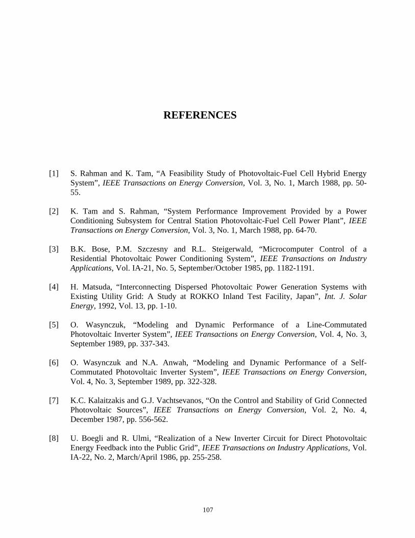
107

REFERENCES

[1] S. Rahman and K. Tam, “A Feasibility Study of Photovoltaic-Fuel Cell Hybrid EnergySystem”, IEEE Transactions on Energy Conversion, Vol. 3, No. 1, March 1988, pp. 50-55.

[2] K. Tam and S. Rahman, “System Performance Improvement Provided by a PowerConditioning Subsystem for Central Station Photovoltaic-Fuel Cell Power Plant”, IEEETransactions on Energy Conversion, Vol. 3, No. 1, March 1988, pp. 64-70.

[3] B.K. Bose, P.M. Szczesny and R.L. Steigerwald, “Microcomputer Control of aResidential Photovoltaic Power Conditioning System”, IEEE Transactions on IndustryApplications, Vol. IA-21, No. 5, September/October 1985, pp. 1182-1191.

[4] H. Matsuda, “Interconnecting Dispersed Photovoltaic Power Generation Systems withExisting Utility Grid: A Study at ROKKO Inland Test Facility, Japan”, Int. J. SolarEnergy, 1992, Vol. 13, pp. 1-10.

[5] O. Wasynczuk, “Modeling and Dynamic Performance of a Line-CommutatedPhotovoltaic Inverter System”, IEEE Transactions on Energy Conversion, Vol. 4, No. 3,September 1989, pp. 337-343.

[6] O. Wasynczuk and N.A. Anwah, “Modeling and Dynamic Performance of a Self-Commutated Photovoltaic Inverter System”, IEEE Transactions on Energy Conversion,Vol. 4, No. 3, September 1989, pp. 322-328.

[7] K.C. Kalaitzakis and G.J. Vachtsevanos, “On the Control and Stability of Grid ConnectedPhotovoltaic Sources”, IEEE Transactions on Energy Conversion, Vol. 2, No. 4,December 1987, pp. 556-562.

[8] U. Boegli and R. Ulmi, “Realization of a New Inverter Circuit for Direct PhotovoltaicEnergy Feedback into the Public Grid”, IEEE Transactions on Industry Applications, Vol.IA-22, No. 2, March/April 1986, pp. 255-258.

108

[9] E.J. Simburger and R.B. Fling, “Engineering Design for a Central Station PhotovoltaicPower Plant”, IEEE Transactions on Power Apparatus and Systems, Vol. PAS-102, No.6, June 1983, pp. 1668-1677.

[10] S.M. Chalmers, P.M. Anderson and P.L. Vogt, “The Effect of Photovoltaic PowerGeneration on Utility Operation”, IEEE Transactions on Power Apparatus and Systems,Vol. PAS-104, No. 3, March 1985, pp. 524-530.

[11] F. Lasnier and T.G. Ang, Photovoltaic Engineering Handbook, The Adam Hilger, 1990.

[12] Y. Hamakawa, “Recent Advances in Solar Photovoltaic Technology and Its New Role forEnvironmental Issue”, Renewable Energy, Vol. 5, Part I, pp. 34-43, 1994.

[13] B.H. Chowdhury and S. Rahman, “Analysis of Interrelationships Between PhotovoltaicPower and Battery Storage for Electric Utility Load Management”, IEEE Transactions onPower Systems, Vol. 3, No. 3, August 1988, pp. 900-907.

[14] G. Smith, Storage Batteries - Including Operation, Charging, Maintenance and Repair,Pitman Advanced Publishing Program, 1980.

[15] K. Tam, P. Kumar and M. Foreman, “Enhancing the Utilization of Photovoltaic PowerGeneration by Superconductive Magnetic Energy Storage”, IEEE Transactions on EnergyConversion, Vol. 4, No. 3, September 1989, pp. 314-321.

[16] H. Schaefer and G. Hagedorn, “Hidden Energy and Correlated EnvironmentalCharacteristics of PV Power Generation”, Renewable Energy, Vol. 2, No. 2, pp. 159-166,1992.

[17] M. Ohnishi and A. Takeoka, “Advanced Photovoltaic Technologies and ResidentialApplications”, Renewable Energy, Vol. 6, No. 3, pp. 275-282, 1995.

[18] A. Chaurey and S. Deambi, “Battery Storage for PV Power Systems: An Overview”,Renewable Energy, Vol. 2, No. 3, pp. 227-235, 1992.

[19] L.J. Blomen and M.N. Mugerwa, Fuel Cell Systems, Plenum Press, New York, 1993

[20] T.M. Calloway, “Autonomous Photovoltaic-Diesel Power System Design”, Proc. IEEEPV Specialists Conference, Las Vegas, Nevada, October 1985, pp. 280-284.

[21] T. Hiyama, S. Kouzuma and T. Imakubo, “Identification of Optimal Operating Point ofPV Modules using Neural Network for Real Time Maximum Power Tracking Control”,IEEE Transactions on Energy Conversion, Vol. 10, No. 2, June 1995, pp. 360-367.

109

[22] T. Hiyama, S. Kouzuma and T. Imakubo, “Evaluation of Neural Network Based RealTime Maximum Power Tracking Controller for PV System”, IEEE Transactions onEnergy Conversion, Vol. 10, No. 3, September 1995, pp. 543-548.

[23] W.J. Lueckel, L.G. Eklund and S.H. Law, “Fuel Cells for Dispersed Power Generation”,IEEE Transactions on Power Apparatus and Systems, Vol. PAS-92, No. 1, January 1973,pp. 230-236.

[24] R.A. Fernandes and H.D. Philipp, “Hydrogen Cycle Peak-Shaving on the New York StateGrid Using Fuel Cells”, IEEE Transactions on Power Apparatus and Systems, Vol. PAS-96, No. 2, March 1977, pp. 467-477.

[25] R.M. Reinstrom, “Carbonate Fuel Cell Power Plant Systems”, IEEE Transactions onPower Apparatus and Systems, Vol. PAS-100, No. 12, December 1981, pp. 4752-4758.

[26] R.A. Bell and R.B. Hayman, “The Electric Utility 4.5 MW Fuel Cell Power Plant - AnUrban Demonstration”, IEEE Transactions on Power Apparatus and Systems, Vol. PAS-100, No. 12, December 1981, pp. 4760-4764.

[27] D.M. Rigney et al., “Expansion Planning with Dispersed Fuel Cell Power Plants onActual Utility Systems”, IEEE Transactions on Power Apparatus and Systems, Vol. PAS-103, No. 9, September 1984, pp. 2388-2393.

[28] S. Matsumoto et al., “Performance Model of Molten Carbonate Fuel Cell”, IEEETransactions on Energy Conversion, Vol. EC-5, No. 2, June 1990, pp. 252-257.

[29] T. Shinoki, M. Matsumoto and A. Sasaki, “Development of an Internal Reforming MoltenCarbonate Fuel Cell Stack”, IEEE Transactions on Energy Conversion, Vol. EC-10, No.4, December 1995, pp. 722-728.

[30] J.W. Beck et al., “A Computer Study of Battery Energy Storage and Power ConversionEquipment Operation”, IEEE Transactions on Power Apparatus and Systems, Vol. PAS-95, No. 4, July 1976, pp. 1064-1072.

[31] H.J. Kunisch, K.G. Kramer and H. Dominik, “Battery Energy Storage: Another Optionfor Load-Frequency-Control and Instantaneous Reserve”, IEEE Transactions on EnergyConversion, Vol. EC-1, No. 3, September 1986, pp. 41-46.

[32] J. Abraham et al., “Balance of Plant Considerations for Load-Leveling Batteries”, IEEETransactions on Energy Conversion, Vol. EC-1, No. 2, June 1986, pp. 131-136.

110

[33] M.W. Migliaro, “Installation Design for Valve-Regulated Sealed Lead-Acid Batteries inGenerating Stations”, IEEE Transactions on Energy Conversion, Vol. 4, No. 1, March1989, pp. 20-24.

[34] J.W. Hurwitch and C.A. Carpenter, “Technology and Application Options for FutureBattery Power Regulation”, IEEE Transactions on Energy Conversion, Vol. 6, No. 1,March 1991, pp. 216-223.

[35] G.M. Cook, W.C. Spindler and G.Grefe, “Overview of Battery Power Regulation andStorage”, IEEE Transactions on Energy Conversion, Vol. 6, No. 1, March 1991, pp. 204-211.

[36] M.A. Casacca and Z.M. Salameh, “Determination of Lead-Acid Battery Capacity viaMathematical Modeling Techniques”, IEEE Transactions on Energy Conversion, Vol. 7,No. 3, September 1992, pp. 442-446.

[37] Z.M. Salameh, M.A. Casacca and W.A. Lynch, “A Mathematical Model for Lead-AcidBatteries”, IEEE Transactions on Energy Conversion, Vol. 7, No. 1, March 1992, pp. 93-97.

[38] D. Kottick, M. Blau and D. Edelstein, “Battery Energy Storage for Frequency Regulationin an Island Power System”, IEEE Transactions on Energy Conversion, Vol. 8, No. 3,September 1993, pp. 455-458.

[39] G.J. Ball, G. Corey and B.L. Norris, “Government, Industry, and Utility Development andEvaluation of a Modular Utility Battery Energy Storage System”, IEEE Transactions onEnergy Conversion, Vol. 10, No. 3, September 1995, pp. 549-554.

[40] C. Lu, C. Liu and C. Wu, “Effect of Battery Energy Storage System on Load FrequencyControl Considering Governor Deadband and Generation Rate Constraint”, IEEETransactions on Energy Conversion, Vol. 10, No. 3, September 1995, pp. 555-561.

[41] R. Ramakumar, H.J. Allison and W.L. Hughes, “Solar Energy Conversion and StorageSystems for the Future”, IEEE Transactions on Power Apparatus and Systems, Vol. PAS-94, No. 6, November 1975. pp 1926-1934.

[42] G.L. Campen, “An Analysis of the Harmonics and Power Factor Effects at a UtilityIntertied Photovoltaic System”, IEEE Transactions on Power Apparatus and Systems,Vol. PAS-101, No. 12, December 1982, pp. 4632-4639.

[43] O. Wasynczuk, “Dynamic Behavior of a Class of Photovoltaic Power Systems”, IEEETransactions on Power Apparatus and Systems, Vol. PAS-102, No. 9, September 1983,pp. 3031-3037.

111

[44] R.C. Dugan, W.T. Jewell and D.J. Roesler, “Harmonics and Reactive Power from Line-Commutated Inverters in Proposed Photovoltaic Subdivision”, IEEE Transactions onPower Apparatus and Systems, Vol. PAS-102, No. 9, September 1983, pp. 3205-3210.

[45] B.W. McNeill and M.A. Mirza, “Estimated Power Quality for Line CommutatedPhotovoltaic Residential System”, IEEE Transactions on Power Apparatus and Systems,Vol. PAS-102, No. 10, October 1983, pp. 3288-3295.

[46] C.M. Ong, “Operational Behavior of Line-Commutated Photovoltaic Systems on aDistribution Feeder”, IEEE Transactions on Power Apparatus and Systems, Vol. PAS-103, No. 8, August 1984, pp. 2262-2268.

[47] P.P. Groumpos, R.C. Cull and A.F. Ratajczak, “An Overview of Control Aspects of aVillage Stand-Alone Photovoltaic Power System”, IEEE Transactions on PowerApparatus and Systems, Vol. PAS-103, No. 10, October 1984, pp. 2845-2853.

[48] M.A. Khallat and S. Rahman, “A Probabilistic Approach to Photovoltaic GeneratorPerformance Prediction”, IEEE Transactions on Energy Conversion, Vol. EC-1, No. 3,September 1986, pp. 34-40.

[49] M.A. Khallat and S. Rahman, “A Model for Capacity Credit Evaluation of Grid-Connected Photovoltaic Systems with Fuel Cell Support”, IEEE Transactions on PowerSystems, Vol. 3, No. 3, August 1988, pp. 1270-1276.

[50] S. Rahman, “Economic Impact of Integrating Photovoltaics with Conventional ElectricUtility Operation”, IEEE Transactions on Energy Conversion, Vol. 5, No. 3, September1990, pp. 422-428.

[51] M.G. Jaboori, M.M. Saied and A.A. Hanafy, “A Contribution to the Simulation andDesign Optimization of Photovoltaic Systems”, IEEE Transactions on EnergyConversion, Vol. 6, No. 3, September 1991, pp. 401-406.

[52] S. Rahman and B.D. Kroposki, “Photovoltaics and Demand Side ManagementPerformance Analysis at a University Building”, IEEE Transactions on EnergyConversion, Vol. 8, No. 3, September 1993, pp. 491-498.

[53] S. Rahman and M. Bouzguenda, “A Model to Determine the Degree of Penetration andEnergy Cost of Large Scale Utility Interactive Photovoltaic Systems”, IEEE Transactionson Energy Conversion, Vol. 9, No. 2, June 1994, pp. 224-230.

[54] N. Mohan, T.M. Undeland and W.P. Robbins, Power Electronics: Converters,Applications, and Design, John Willey & Sons, 1989.

112

[55] L.H. Michaels, B.T. Fairchild and S.T. Kohn, “Hybrid Simulation of Fuel Cell PowerConversion Systems”, IEEE Transactions on Power Apparatus and Systems, Vol. PAS-96, No. 4, July 1977, pp. 1329-1336.

[56] G.E. Gareis et al., “The Interactionof Batteries and Fuel Cells with Electrical DistributionSystems: Force Commutated Converter Interface”, IEEE Transactions on PowerApparatus and Systems, Vol. PAS-96, No. 4, July 1977, pp. 1242-1250.

[57] D.P. Carroll et al., “The Interactionof Batteries and Fuel Cells with Electrical DistributionSystems: Line Commutated Converter Interface”, IEEE Transactions on Power Apparatusand Systems, Vol. PAS-96, No. 4, July 1977, pp.1202-1210.

[58] G.A. Phillips, J.W. Walton and F.J. Kornbrust, “Progress in Self-Commutated Invertersfor Fuel Cells and Batteries”, IEEE Transactions on Power Apparatus and Systems, Vol.PAS-98, No. 4, July 1979, pp. 1466-1475.

[59] P.K. Simpson, “Foundations of Neural Networks”, Proceedings of the Adaptive ControlSystems Technology Symposium, October 24-25, 1994, pp. 16-37.

[60] D.J. Sobajic and Y.H. Pao, “Artificial Neural-Net Based Dynamic Security Assessmentfor Electric Power Systems”, IEEE Transactions on Power Systems, Vol. 4, No. 1,February 1989, pp. 220-226.

[61] C.R. Chen and Y.Y. Hsu, “Synchronous Machine Steady-State Stability Analysis using anArtificial Neural Network”, IEEE Transactions on Energy Conversion, Vol. 6, No. 1,March 1991, pp. 12-20.

[62] Y.Y. Hsu and C.R. Chen, “Tuning of Power System Stabilizers using an Artificial NeuralNetwork”, IEEE Transactions on Energy Conversion, Vol. 6, No. 4, December 1991, pp.612-619.

[63] M. Aggoune et al., “Preliminary Results on Using Artificial Neural Networks for SecurityAssessment”, IEEE Transactions on Power Systems, Vol. 6, No. 2, May 1991, pp. 890-896.

[64] K. Ikenono and S. Iwamoto, “Generalization of Transient Stability Solution Using NeuralNetwork Theory”, Electrical Engineering in Japan, Vol. 112, No. 3, 1992, pp. 72-79.

[65] M. Djukanovic, D.J. Sobajic and Y.H. Pao, “Neural Net Based Determination ofGenerator-Shedding Requirements in Electric Power Systems”, IEE Proceedings -C, Vol.139, No. 5, September 1992, pp. 427-436.

113

[66] N. Kandil et al., “Fault Identification in an AC-DC Transmission System Using NeuralNetworks”, IEEE Transactions on Power Systems, Vol. 7, No. 2, May 1992, pp. 812-818.

[67] H. Mori, Y. Tamaru and S. Tsuzuki, “An Artificial Neural-Net Based Technique forPower System Dynamic Stability with the Kohonen Model”, IEEE Transactions on PowerSystems, Vol. 7, No. 2, May 1992, pp. 856-864.

[68] D. Niebur and A.J. Germond, “Power System Static Security Assessment Using theKohonen Neural Network Classifier”, IEEE Transactions on Power Systems, Vol. 7, No.2, May 1992, pp. 865-872.

[69] H. Sasaki, M. Watanabe and R. Yokoyama, “A Solution Method of Unit Commitment byArtificial Neural Networks”, IEEE Transactions on Power Systems, Vol. 7, No. 3, August1992, pp. 974-980.

[70] Y.Y. Hsu and L.H. Jeng, “Analysis of Torsional Oscillations Using an Artificial NeuralNetwork”, IEEE Transactions on Energy Conversion, Vol. 7, No. 4, December 1992, pp.684-690.

[71] T. Sorsa and H.N. Koivo, “Application of Artificial Neural Networks in Process FaultDiagnosis”, Automatica, Vol. 29, No. 4, 1993, pp. 843-849.

[72] Y. Zhang, O.P. Malik and G.P. Chen, “Artificial Neural Network Power SystemStabilizers in Multi-Machine Power System Environment”, IEEE Transactions on EnergyConversion, Vol. 10, No. 1, March 1995, pp. 147-153.

[73] K.H. Abdul-Rahman, S.M. Shahidhpour and M. Daneshdoost, “AI Approach to OptimalVAR Control with Fuzzy Reactive Loads”, IEEE Transactions on Power Systems, Vol.10, No. 1, February 1995, pp. 88-97.

[74] A.G. Bakirtzis et al., “Short Term Load Forecasting Using Fuzzy Neural Networks”,IEEE Transactions on Power Systems, Vol. 10, No. 3, August 1995, pp. 1518-1524.

[75] T. Denise King, M.E. El-Hawary and F. El-Hawary, “Optimal Environmental Dispatchingof Electric Power Systems via an Improved Hopfield Neural Network Model”, IEEETransactions on Power Systems, Vol. 10, No. 3, August 1995, pp. 1559-1564.

[76] A.A. El-Keib and X. Ma, “Application of Artificial Neural Networks in Voltage StabilityAssessment”, IEEE Transactions on Power Systems, Vol. 10, No. 4, November 1995, pp.1890-1896.

114

[77] T.S. Sidhu and Z. Ao, “On-Line Evaluation of Capacity and Energy Losses in PowerTransmission Systems by Using Artificial Neural Networks”, IEEE Transactions onPower Delivery, Vol.107, No. 4, October 1995, pp. 1913-1919.

[78] R. Noyes (ed.), Fuel Cells for Public Utility and Industrial Power, Noyes DataCorporation, 1977.

[79] M. Hsu, “Ztek’s Ultra-High Efficiency Fuel Cell/Gas Turbine System for DistributedGeneration”, 1996 Fuel Cell Seminar, Nov. 17-20, 1996, Orlando, Florida, pp. 183-186.

[80] R.C. Ruhl, M.A. Petrik and T.L. Cable, “Status of the TMI Systems”, 1996 Fuel CellSeminar, Nov. 17-20, 1996, Orlando, Florida, pp. 187-189.

[81] G. Marland, “Carbon Dioxide Emission Rates for Conventional and Synthetic Fuels”,Energy, Vol. 8, No. 12, 1983, pp. 981-992.

[82] OECD, Environmental Effects of Electricity Generation, OECD Publications Office,1985.

[83] F. Kreith, P. Norton and D. Brown, “A Comparison of CO2 Emissions from Fossil andSolar Power Plants in the United States”, Energy, Vol. 15, No. 12, 1990, pp. 1181-1198.

[84] “Fedral Technology Alert - Natural Gas Fuel Cells”, 1996, http://w3.pnl.gov:2080/fta/5_nat.htm.

[85] Technology Transition Corporation, “The Entry Market for Fuel Cells”, 1996,http://www. ttcorp.com/fccg/fcmabstr.htm.

[86] K. Jung, H. Kim and D. Rho, “Determination of the Installation Site and OptimalCapacity of the Battery Energy Storage System for Load Leveling”, IEEE Transactionson Energy Conversion, Vol. 11, No. 1, March 1996, pp. 162-167.

[87] J.G. Kassakian, M.F. Schlecht and G.C. Verghese, Principles of Power Electronics,Addison-Wesley Publishing Company, 1991.

[88] N. Argaw, “Optimization of Photovoltaic Water Pumps Coupled with an Interfacing PulseWidth Modulated DC/AC Inverter Power Conditioning Device”, 1994 IEEE First WorldConference on Photovoltaic Energy Conversion, Dec. 5-9, 1994, Hawii, pp. 1165-1168.

[89] R. Naik et al., “A Novel Grid Interface, Optimized for Utility-Scale Applications ofPhotovoltaic, Wind-Electric, and Fuel-Cell Systems”, ”, IEEE Transactions on PowerDelivery, Vol. 10, No. 4, October 1995, pp. 1920-1926.

115

[90] W. Shireen and M.S. Arefeen, “An Utility Interactive Power Electronics Interface forAlternate/Renewable Energy Systems”, ”, IEEE Transactions on Energy Conversion, Vol.11, No. 3, September 1996, pp. 643-648.

[91] A.J. Appleby, Fuel Cells: Trends in Research and Applications, Hemisphere PublishingCorporation, 1987.

116

APPENDIX. A

CO2 EMISSIONS FROM CONVENTIONAL FOSSIL FUEL

POWER PLANTS

CO2 emission rates in terms of kgCO2/MWh for three conventional fossil fuel (coal, oil,and natural gas) power plants during their operations are computed. The following reactionsmay represent the complete combustion of fossil fuel at power plants.

C O CO+ → +2 2 ∆ (A.1)

or CH O CO H O4 2 2 22 2+ → + + ∆ (A.2)

where ∆ represents heat evolved. The CO2 emissions shown in Equation (A.1) - (A.2) areconsidered as an undesirable side effect of burning fossil fuel to get useful energy.

For the CO2 emission rate of coal combustion, Appalachian bituminous coal with 72%carbon content and 12,600 Btu/lb (29.347x 109 J/ton) of heating value is taken as arepresentative. The CO2 emission rate for complete combustion of the coal is computed as

072 1029 347 10

24 534 10 323 8233

99

2..

. / . /×

×= =

kgCJ

kgC J kgCO MWh

When the power plant has a 34% of electricity conversion efficiency, the CO2 release rate wouldbe 952.42 kgCO2/MWh.

An emission rate for crude oil can be calculated from its composition, heating value, andefficiency of a power plant. The United Nations uses 1.4543 ton of coal equivalent to define aton of oil equivalent and average crude oil is characterized as having 85.0 ± 1.0% carbon content.The CO2 emission rate for complete combustion of crude oil is computed as follows

117

0 85 1014543 29 347 10

19 916 10 262 873

99

2.

. .. / . /

×× ×

= =kgC

JkgC J kgCO MWh

Then assuming 37% of electricity conversion efficiency, the CO2 release rate would be 710.46kgCO2/MWh.

When natural gas is roughly assumed to contain 100% methane (CH4), whose heatingvalue is 23,861 Btu/lb (55.5756x109 J/ton), the CO2 emission rate for methane is calculated as

075 1055 5756 10

13 50 103

99.

.. /

××

=kgC

JkgC J

However, the average natural gas used in power plants contains 92.88% methane, 3.91% ethane(C2H6), a small amount of propane (C3H8) and other non-hydrocarbon gases, for a heating valueof 9103 kcal/m3. Considering the kinds of variability, the relation between carbon content andheating value of natural gas is approximated by the following equation

kgC/109J = 13.71 + [(kcal/m3) x 0.1124 - 1000] x 3.083x10-3

For the average natural gas, this value is 13.78 kgC/109J (181.88 kg CO2/MWh). Taking 39% asthe efficiency of the natural gas power plant, the CO2 emission rate would be 466.36kgCO2/MWh.

On the other hand, before each fuel is combusted at power plants, it is required to beprocessed at a fuel treatment stage. The fuel treatment processes usually consist of mining,transportation and refining of fossil fuel. Taking the CO2 generation from the fuel treatment intoaccount, Table A.1 summarizes the overall CO2 emissions of the three fossil fuel power plants.

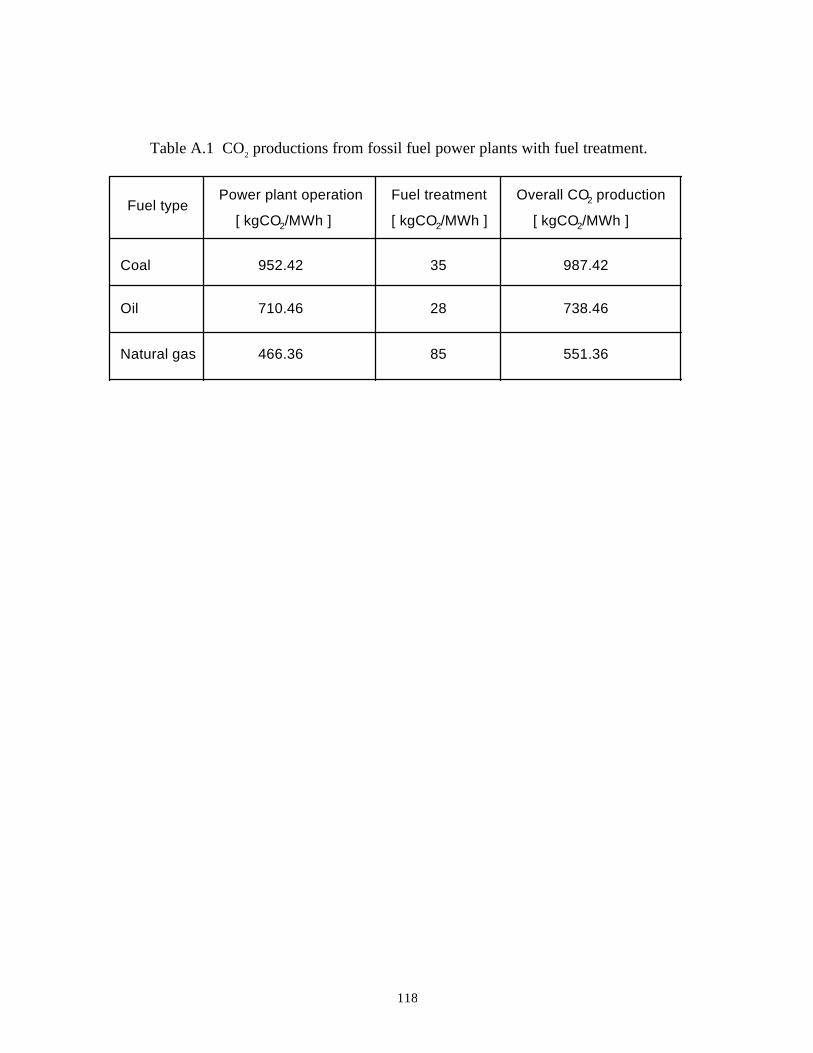
118

Table A.1 CO2 productions from fossil fuel power plants with fuel treatment.

Fuel typePower plant operation

[ kgCO2/MWh ]

Fuel treatment

[ kgCO2/MWh ]

Overall CO2 production

[ kgCO2/MWh ]

Coal

Oil

Natural gas

952.42

710.46

466.36

35

28

85

987.42

738.46

551.36

119

APPENDIX. B

CO2 EMISSIONS FROM PV POWER PLANTS

This section calculates estimates of the CO2 emissions from both PV module fabricationand construction of the PV power plant, based on consumed energy analysis.

Accumulated energy requirements for construction of PV power plants are shown inTable B.1 [16]. The energy consumed for the photovoltaic modules and that for the remainingcomponents such as supporting structures, cabling, power conditioning system, etc. constitutethe accumulated energy for a PV power plant. The percentages by which electrical energy andraw fuel take charge out of the total energy consumption are 68.2% and 28.8%, respectively.

Table B.1 Accumulated energy requirements for PV power plants [16].

Cell structure

- Size of power station = 1,500 kWp- Annual production capacity = 25 MWp/yr

η Remainingcomponents[kWh/kWp]

Power stationtotal[kWh/kWp]

PV Modules

[kWh/kWp][%]

Single-crystalline

Poly-crystalline

Amorphous

15.5

13.5

8.0

11,000 1,200 12,200

7,500 1,500 9,000

5,500 2,000 7,500

120

CO2 emissions, involved in the construction process of the PV power plant by theconsumption of electricity and fuels, can be estimated using the specific emission factors withinan energy supply network. For the United States, 0.5984 kg/kWh for electrical energy and 0.48kg/kWh for fossil fuels are calculated for their CO2 emission factors. These calculations arebased on the data that the percentage of electricity generated by coal is 54.6%, by oil 3.9%, andby natural gas 11.9%. The emission factors for coal, oil and natural gas power plants are 952.42kg/MWh, 710.46 kg/MWh, and 466.36 kg/MWh, respectively, as calculated in Appendix A.Table B.2 shows the amount of CO2 emitted during the construction of the PV power plant andequivalent CO2 emissions during the system’s working life cycle.

Table B.2. CO2 emissions of PV power plants.

Cell structureCO2 emissions

[ kg CO2/kWp ]

Equivalent CO2 emissions[ kg CO2/MWh ]

Single- crystalline

Poly-crystalline

Amorphous

6,654.5

4,909.1

4090.9

110.9

81.8

68.2

- Working life cycle = 30 yrs- Annual load duration = 2,000 hrs

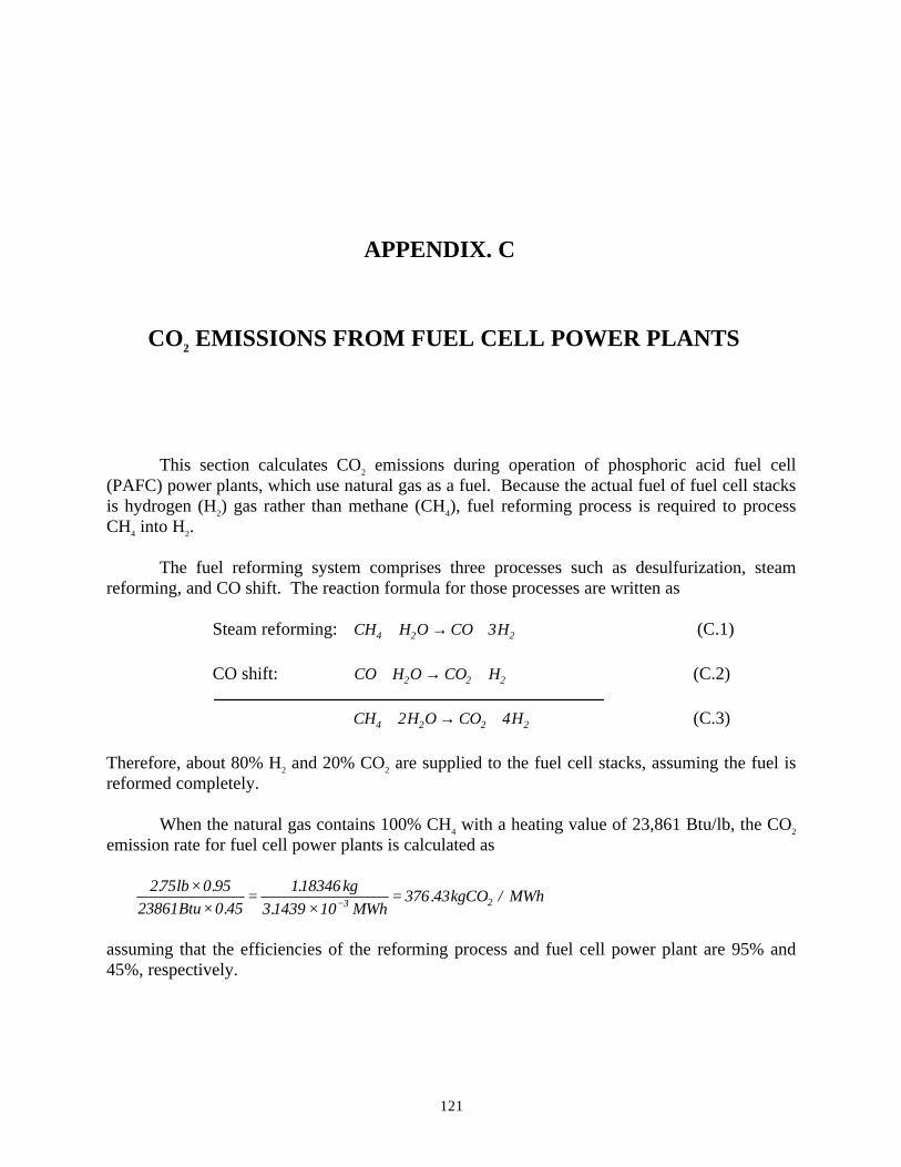
121

APPENDIX. C

CO2 EMISSIONS FROM FUEL CELL POWER PLANTS

This section calculates CO2 emissions during operation of phosphoric acid fuel cell(PAFC) power plants, which use natural gas as a fuel. Because the actual fuel of fuel cell stacksis hydrogen (H2) gas rather than methane (CH4), fuel reforming process is required to processCH4 into H2.

The fuel reforming system comprises three processes such as desulfurization, steamreforming, and CO shift. The reaction formula for those processes are written as

Steam reforming: CH H O CO H4 2 23+ → + (C.1)

CO shift: CO H O CO H+ → +2 2 2 (C.2)

CH H O CO H4 2 2 22 4+ → + (C.3)

Therefore, about 80% H2 and 20% CO2 are supplied to the fuel cell stacks, assuming the fuel isreformed completely.

When the natural gas contains 100% CH4 with a heating value of 23,861 Btu/lb, the CO2

emission rate for fuel cell power plants is calculated as

275 0 95

23861 0 45118346

3 1439 10376 433 2

. ..

..

. /lbBtu

kgMWh

kgCO MWh×

×=

×=−

assuming that the efficiencies of the reforming process and fuel cell power plant are 95% and45%, respectively.

122

VITA

Kyoungsoo Ro

He was born on March 27, 1963, in Changnyung, Korea. He obtained his B.S. and M.S.degrees in Electrical Engineering from the Seoul National University, Korea in 1985 and 1987,respectively. He had finished course-works for his Ph.D. study at the Seoul National Universityin 1990. In the Fall of 1993, he joined the Virginia Polytechnic Institute and State University(Virginia Tech) to pursue his Ph.D. He has worked as a teaching assistant since 1994 and hastaught the Power Engineering Laboratory since the Fall of 1995. He is supposed to obtain hisdoctorate degree on May 9, 1997. His interest areas are power system operation, control andstability, renewable energy systems (photovoltaics, fuel cells and batteries) and applications ofartificial intelligence to power systems. He has been a member of Institute of Electrical andElectronics Engineers (IEEE) since 1995.

April 14, 1997