Maximizing Resource Utilization In Video Streaming Systems

Wayne State University

Wayne State University Dissertations

1-1-2013

Maximizing Resource Utilization In VideoStreaming SystemsMohammad A. AlsmiratWayne State University,

Follow this and additional works at: http://digitalcommons.wayne.edu/oa_dissertations

Part of the Communication Commons, and the Computer Engineering Commons

This Open Access Dissertation is brought to you for free and open access by DigitalCommons@WayneState. It has been accepted for inclusion inWayne State University Dissertations by an authorized administrator of DigitalCommons@WayneState.

Recommended CitationAlsmirat, Mohammad A., "Maximizing Resource Utilization In Video Streaming Systems" (2013). Wayne State University Dissertations.Paper 630.

http://digitalcommons.wayne.edu/?utm_source=digitalcommons.wayne.edu%2Foa_dissertations%2F630&utm_medium=PDF&utm_campaign=PDFCoverPages

http://digitalcommons.wayne.edu/?utm_source=digitalcommons.wayne.edu%2Foa_dissertations%2F630&utm_medium=PDF&utm_campaign=PDFCoverPages

http://digitalcommons.wayne.edu/oa_dissertations?utm_source=digitalcommons.wayne.edu%2Foa_dissertations%2F630&utm_medium=PDF&utm_campaign=PDFCoverPages

http://digitalcommons.wayne.edu/oa_dissertations?utm_source=digitalcommons.wayne.edu%2Foa_dissertations%2F630&utm_medium=PDF&utm_campaign=PDFCoverPages

http://network.bepress.com/hgg/discipline/325?utm_source=digitalcommons.wayne.edu%2Foa_dissertations%2F630&utm_medium=PDF&utm_campaign=PDFCoverPages

http://network.bepress.com/hgg/discipline/258?utm_source=digitalcommons.wayne.edu%2Foa_dissertations%2F630&utm_medium=PDF&utm_campaign=PDFCoverPages

http://digitalcommons.wayne.edu/oa_dissertations/630?utm_source=digitalcommons.wayne.edu%2Foa_dissertations%2F630&utm_medium=PDF&utm_campaign=PDFCoverPages

MAXIMIZING RESOURCE UTILIZATION IN VIDEO STREAMING SYSTEMS

by

MOHAMMAD ABDULLAH ALSMIRAT

DISSERTATION

Submitted to the Graduate School

of Wayne State University,

Detroit, Michigan

in partial fulfillment of the requirements

for the degree of

DOCTOR OF PHILOSOPHY

2013

MAJOR: COMPUTER ENGINEERING

Approved by:

Advisor Date

ACKNOWLEDGMENTS

I have taken great efforts in this research. However, it would not have been possible without the kind

support and help of many people.

I would like to thank my advisor Dr. Nabil Sarhan for his continuous guidance and support. I also

would like to thank my PhD committee Dr. Cheng-Zhong Xu, Dr. Syed Mahmud, and Dr. Nathan Fisher

for their valuable input.

I wish to dedicate this work to my beloved parents who always supported me and without their

blessings I would not have achieved this work. I also wish to express my love and unlimited gratitude to

my beloved family; my wife Hend, my daughter Zainah, and my two sons Hamzah and Amjad, for their

understanding, support, motivation, and endless love through the duration of my study. Finally, I would

like to thank my brothers, my sisters, and my friends for their continuous support.

ii

TABLE OF CONTENTS

Acknowledgments . . . . . . . . . . . . . . . . . . . . . . . . . . . . . . . . . . . . . . . . . . ii

List of Tables . . . . . . . . . . . . . . . . . . . . . . . . . . . . . . . . . . . . . . . . . . . . .viii

List of Figures . . . . . . . . . . . . . . . . . . . . . . . . . . . . . . . . . . . . . . . . . . . .ix

CHAPTER 1 INTRODUCTION . . . . . . . . . . . . . . . . . . . . . . . . . . . . . . . . . 1

1.1 Motivation . . . . . . . . . . . . . . . . . . . . . . . . . . . . . . . . . . . . . . . . . .1

1.2 Overview . . . . . . . . . . . . . . . . . . . . . . . . . . . . . . . . . . . . . . . . . .1

1.3 Proposed Work on VOD Systems . . . . . . . . . . . . . . . . . . . . . . . . . . .. . . 3

1.4 Proposed Work on AVS Systems . . . . . . . . . . . . . . . . . . . . . . . . . . .. . . 6

CHAPTER 2 BACKGROUND INFORMATION AND RELATED WORK . . . . . . . . . 9

2.1 Main Performance Metrics of Video Streaming Systems . . . . . . . . . . . . . .. . . . 9

2.2 Scalable Delivery of Video Streams with Stream Merging . . . . . . . . . . . .. . . . . 9

2.3 Request Scheduling of Waiting Video Requests . . . . . . . . . . . . . . . . .. . . . . 11

2.4 IEEE 802.11e Standard . . . . . . . . . . . . . . . . . . . . . . . . . . . . . . . .. . . 13

2.5 Cross-Layer Optimization in Video Streaming Systems . . . . . . . . . . . . . . . .. . 14

2.5.1 Automated Video Surveillance . . . . . . . . . . . . . . . . . . . . . . . . . . . 15

2.6 Effective Airtime Estimation . . . . . . . . . . . . . . . . . . . . . . . . . . . . . . . . 16

CHAPTER 3 INCREASING SYSTEM BANDWIDTH UTILIZATION BY USING WAITING-

TIME PREDICTION IN VIDEO-ON-DEMAND SYSTEMS . . . . . . . . . 17

3.1 Introduction . . . . . . . . . . . . . . . . . . . . . . . . . . . . . . . . . . . . . . . .. 17

3.2 Providing Time-of-Service Guarantees . . . . . . . . . . . . . . . . . . . . .. . . . . . 19

3.3 Proposed Waiting-Time Prediction Approach . . . . . . . . . . . . . . . . . . .. . . . 22

iii

3.3.1 Proposed AEC Scheme . . . . . . . . . . . . . . . . . . . . . . . . . . . . . . . 23

3.3.2 Proposed Enhancements of AEC . . . . . . . . . . . . . . . . . . . . . . . . .. 27

3.3.3 Feedback Control of the Prediction Window . . . . . . . . . . . . . . . . . .. . 28

3.3.4 Proposed Hybrid Prediction Scheme . . . . . . . . . . . . . . . . . . . . . . .. 30

3.4 Evaluation Methodology . . . . . . . . . . . . . . . . . . . . . . . . . . . . . . . . .. 31

3.4.1 Workload Characteristics . . . . . . . . . . . . . . . . . . . . . . . . . . . . . .31

3.4.2 Performance Metrics . . . . . . . . . . . . . . . . . . . . . . . . . . . . . . . . 32

3.5 Result Presentation and Analysis . . . . . . . . . . . . . . . . . . . . . . . . . .. . . . 33

3.5.1 Waiting-Time Distribution under Various Scheduling Policies . . . . . . . . . .33

3.5.2 Waiting-Time Predictability and Effectiveness of Various Prediction Schemes . . 34

3.5.3 Effectiveness of Further Enhancements . . . . . . . . . . . . . . . . . .. . . . 35

3.5.4 Impact of Prediction Window . . . . . . . . . . . . . . . . . . . . . . . . . . . 36

3.5.5 Analysis of Deviation Distributions under Various Prediction Schemes . .. . . . 38

3.5.6 Impact of Workload Parameters on AEC Performance . . . . . . . . . . .. . . 38

3.5.7 Feedback Control of the Prediction Window in AEC . . . . . . . . . . . . . .. 41

3.5.8 Effectiveness of the Waiting-Time Prediction Approach Compared with GNSTF 42

3.6 Conclusions . . . . . . . . . . . . . . . . . . . . . . . . . . . . . . . . . . . . . . . .. 44

CHAPTER 4 INCREASING SYSTEM BANDWIDTH UTILIZATION BY ENHANCING

SCHEDULING DECISIONS IN VIDEO-ON-DEMAND SYSTEMS . . . . . 47

4.1 Introduction . . . . . . . . . . . . . . . . . . . . . . . . . . . . . . . . . . . . . . . .. 47

4.2 Analysis of Cost-Based Scheduling . . . . . . . . . . . . . . . . . . . . . . . .. . . . . 48

4.2.1 Lookahead Scheduling . . . . . . . . . . . . . . . . . . . . . . . . . . . . . . .49

4.2.2 Combinational Scheduling . . . . . . . . . . . . . . . . . . . . . . . . . . . . . 49

4.3 Proposed Predictive Cost-Based Scheduling . . . . . . . . . . . . . . . .. . . . . . . . 51

iv

4.4 Proposed Adaptive Regular Stream Triggering (ART) . . . . . . . . . .. . . . . . . . . 53

4.5 Evaluation Methodology . . . . . . . . . . . . . . . . . . . . . . . . . . . . . . . . .. 55

4.5.1 Workload Characteristics . . . . . . . . . . . . . . . . . . . . . . . . . . . . . .56

4.5.2 Considered Performance Metrics . . . . . . . . . . . . . . . . . . . . . . . .. . 57


4.6.1 Comparing the Effectiveness of Different Cost-Computation Alternatives . . . . 57

4.6.2 Effectiveness of the Proposed PCS Policy . . . . . . . . . . . . . . . . .. . . . 58

4.6.3 Effectiveness of the Proposed ART Enhancement . . . . . . . . . . .. . . . . . 59

4.6.4 Comparing the Effectiveness of PCS and ART . . . . . . . . . . . . . . . .. . 62

4.6.5 Impact of Workload Parameters on the Effectiveness of PCS and ART . . . . . . 64

4.6.6 Comparing Waiting-Time Predictability with PCS and ART . . . . . . . . . . . 67

4.6.7 Impact of Flash Crowds on the Effectiveness of PCS and ART . . . .. . . . . . 68

4.6.8 Effectiveness of Combining ART with PCS . . . . . . . . . . . . . . . . . . . .69

4.7 Conclusions . . . . . . . . . . . . . . . . . . . . . . . . . . . . . . . . . . . . . . . .. 70

CHAPTER 5 DISTORTION-BASED CROSS-LAYER OPTIMIZATION FOR WIRELESS

VIDEO STREAMING . . . . . . . . . . . . . . . . . . . . . . . . . . . . . . .72

5.1 Introduction . . . . . . . . . . . . . . . . . . . . . . . . . . . . . . . . . . . . . . . .. 72

5.2 Proposed Cross-Layer Optimization Framework . . . . . . . . . . . . . . . .. . . . . . 75

5.2.1 Cross-Layer Optimization Problem Formulation . . . . . . . . . . . . . . . . . 75

5.2.2 Distortion Function Characterization . . . . . . . . . . . . . . . . . . . . . . . .76

5.2.3 Effective Airtime Estimation . . . . . . . . . . . . . . . . . . . . . . . . . . . . 77

5.2.4 Enhanced Effective Airtime Estimation . . . . . . . . . . . . . . . . . . . . . . 79

5.2.5 Cross-Layer Optimization Solution . . . . . . . . . . . . . . . . . . . . . . . . 80

5.2.6 Enforcing the Optimization Results . . . . . . . . . . . . . . . . . . . . . . . . 81

v

5.3 Performance Evaluation Methodology . . . . . . . . . . . . . . . . . . . . . . .. . . . 83

5.4 Results Presentation and Analysis . . . . . . . . . . . . . . . . . . . . . . . . . .. . . 85

5.4.1 Effectiveness of Using the Cross-Layer Approach in Bandwidth Allocation . . . 85

5.4.2 Analysis of the Enhanced Effective Airtime Estimation Algorithm . . . . . . . . 85

5.4.3 Analysis of Link-Layer Adaptation . . . . . . . . . . . . . . . . . . . . . . . .87

5.4.4 Comparing Various Bandwidth Allocation Solutions . . . . . . . . . . . . . . . 88

5.4.5 Impact of Interfering Traffic on the Performance of the ProposedBandwidth

Allocation Solution . . . . . . . . . . . . . . . . . . . . . . . . . . . . . . . . . 89

5.5 Conclusions . . . . . . . . . . . . . . . . . . . . . . . . . . . . . . . . . . . . . . . .. 91

CHAPTER 6 ACCURACY-BASED CROSS-LAYER OPTIMIZATION FOR AUTOMATED

VIDEO SURVEILLANCE . . . . . . . . . . . . . . . . . . . . . . . . . . . .95

6.1 Introduction . . . . . . . . . . . . . . . . . . . . . . . . . . . . . . . . . . . . . . . .. 95

6.2 Proposed Accuracy-Based Cross-Layer Optimization Framework . .. . . . . . . . . . . 96

6.2.1 Optimization Problem Formulation . . . . . . . . . . . . . . . . . . . . . . . . 97

6.2.2 Rate-Accuracy Characterization . . . . . . . . . . . . . . . . . . . . . . . .. . 98

6.2.3 Effective Airtime Estimation . . . . . . . . . . . . . . . . . . . . . . . . . . . . 101

6.2.4 Optimization Solution . . . . . . . . . . . . . . . . . . . . . . . . . . . . . . . 102

6.2.5 The Allocation Algorithm . . . . . . . . . . . . . . . . . . . . . . . . . . . . . 103

6.2.6 Proposed Bandwidth Pruning Mechanism . . . . . . . . . . . . . . . . . . .. . 104

6.3 Performance Evaluation Methodology . . . . . . . . . . . . . . . . . . . . . . .. . . . 104


6.4.1 Effectiveness of the Proposed Effective Airtime Estimation . . . . . . . .. . . . 106

6.4.2 Effectiveness of the Proposed Bandwidth Allocation Solution . . . . . .. . . . 107

6.4.3 Effectiveness of the Proposed Bandwidth Pruning Mechanism . . .. . . . . . . 108

vi

6.5 Conclusions . . . . . . . . . . . . . . . . . . . . . . . . . . . . . . . . . . . . . . . .. 108

CHAPTER 7 SUMMARY AND FUTURE WORK . . . . . . . . . . . . . . . . . . . . . . .117

7.1 Summary . . . . . . . . . . . . . . . . . . . . . . . . . . . . . . . . . . . . . . . . . . 117

7.1.1 Waiting-time Predictability . . . . . . . . . . . . . . . . . . . . . . . . . . . . . 117

7.1.2 Scheduling . . . . . . . . . . . . . . . . . . . . . . . . . . . . . . . . . . . . . 118

7.1.3 Distortion-based Dynamic Bandwidth Allocation . . . . . . . . . . . . . . . . . 118

7.1.4 Accuracy-based Dynamic Bandwidth Allocation . . . . . . . . . . . . . . . .. 119

7.2 Future Work . . . . . . . . . . . . . . . . . . . . . . . . . . . . . . . . . . . . . . . .. 120

Bibliography . . . . . . . . . . . . . . . . . . . . . . . . . . . . . . . . . . . . . . . . . . . . .121

Abstract . . . . . . . . . . . . . . . . . . . . . . . . . . . . . . . . . . . . . . . . . . . . . . .131

Autobiographical Statement . . . . . . . . . . . . . . . . . . . . . . . . . . . . . . . . . . . .133

vii

L IST OF TABLES

Table 3.1 Summary of Workload Characteristics . . . . . . . . . . . . . . . . . . . .. . . . 32

Table 3.2 Summary of Deviation Distributions [ERMT, MCF-P, 300 Channels, Model A] . . 40

Table 4.1 Summary of Workload Characteristics . . . . . . . . . . . . . . . . . . . .. . . . 56

Table 5.1 Notations Summary . . . . . . . . . . . . . . . . . . . . . . . . . . . . . . . . . 74

Table 5.2 Summary of Simulation Parameters . . . . . . . . . . . . . . . . . . . . . . . . .85

Table 5.3 Impact of the Time Interval Selected to Determine TXOP Limit . . . . . . . .. . 87

Table 6.1 Summary of Simulation Parameters . . . . . . . . . . . . . . . . . . . . . . . . .105

Table 6.2 Summary of PID Parameter Tuning . . . . . . . . . . . . . . . . . . . . . . .. . 106

viii

L IST OF FIGURES

Figure 1.1 Simplified VOD Streaming Environment . . . . . . . . . . . . . . . . . . . . .. 2

Figure 1.2 AVS System Overview . . . . . . . . . . . . . . . . . . . . . . . . . . . . .. . 3

Figure 2.1 Patching . . . . . . . . . . . . . . . . . . . . . . . . . . . . . . . . . . . . . .. 10

Figure 2.2 Transition Patching . . . . . . . . . . . . . . . . . . . . . . . . . . . . . . .. . 10

Figure 2.3 ERMT . . . . . . . . . . . . . . . . . . . . . . . . . . . . . . . . . . . . . . . .10

Figure 3.1 Clarification of GNSTF . . . . . . . . . . . . . . . . . . . . . . . . . . . . .. . 22

Figure 3.2 Simplified Algorithm for the AEC Scheme . . . . . . . . . . . . . . . . . . . .26

Figure 3.3 Clarification of the AEC Scheme . . . . . . . . . . . . . . . . . . . . . . . .. . 27

Figure 3.4 Controllers of Prediction Accuracy . . . . . . . . . . . . . . . . . . .. . . . . . 30

Figure 3.5 Waiting Time Distribution [Patching, 600 Channels, Model A] . . . . . . . . . . 33

Figure 3.6 Comparing the Accuracy of Prediction Schemes [MQL, Wp = 0.5µtol , Model A] . 34

Figure 3.7 Comparing the Accuracy of Prediction Schemes [Wp = 0.5µtol , Model A] . . . . 35

Figure 3.8 Comparing the Accuracy of Prediction Schemes . . . . . . . . . . . .. . . . . . 35

Figure 3.9 Effectiveness of the Preferential Treatment of Real Requests Enhancement . . . . 36

Figure 3.10 Impact of the Periodic Refinement . . . . . . . . . . . . . . . . . . . .. . . . . 36

Figure 3.11 Impact of Prediction Window . . . . . . . . . . . . . . . . . . . . . . . .. . . . 37

Figure 3.12 Impact of Prediction Window on Algorithm Computation Time . . . . . . .. . . 37

Figure 3.13 Comparing the Deviation Distributions under Various Prediction Algorithms . . . 39

Figure 3.14 Comparing the Distributions of the Deviation Percentage . . . . . . .. . . . . . 40

Figure 3.15 Impact of Workload on Average Deviation . . . . . . . . . . . . . .. . . . . . . 41

Figure 3.16 Impact of Workload on PCRE [AEC, 550 Channels, Wp = µtol , Model A] . . . . 42

Figure 3.17 Impact of Variable-Length Video Workloads . . . . . . . . . . . .. . . . . . . . 43

Figure 3.18 Impact of the Shape Parameter of Weibull Arrival Distribution . .. . . . . . . . 43

ix

Figure 3.19 Effectiveness of PID Controller . . . . . . . . . . . . . . . . . . .. . . . . . . . 44

Figure 3.20 Effectiveness of Exponential Controller . . . . . . . . . . . . .. . . . . . . . . 44

Figure 3.21 Comparing GNSTF with Predictive MCF-P [Model B] . . . . . . . .. . . . . . 45

Figure 3.22 Comparing GNSTF with Predictive MCF-P [Model C] . . . . . . . .. . . . . . 45

Figure 3.23 Comparing GNSTF with Predictive MCF-P (Two Variants) . . . . .. . . . . . . 46

Figure 4.1 An Illustration of Lookahead Scheduling . . . . . . . . . . . . . . . .. . . . . . 50

Figure 4.2 Illustration of Combinational Scheduling . . . . . . . . . . . . . . . . . .. . . . 51

Figure 4.3 Simplified Algorithm for Dynamically ComputingfreeChannelThresh. . . . . . 52

Figure 4.4 Simplified Algorithm for PCS-V . . . . . . . . . . . . . . . . . . . . . . . . .. 53

Figure 4.5 Simplified Algorithm for PCS-L . . . . . . . . . . . . . . . . . . . . . . . . .. 54

Figure 4.6 Simplified Implementation of ART . . . . . . . . . . . . . . . . . . . . . . . . . 54

Figure 4.7 Impact of ART on ERMT Stream Merge Tree . . . . . . . . . . . . . .. . . . . 55

Figure 4.8 Effectiveness of Lookahead and Combinational Scheduling [ERMT] . . . . . . . 58

Figure 4.9 Effectiveness of PCS [ERMT] . . . . . . . . . . . . . . . . . . . . . . . . . . . . 59

Figure 4.10 Effectiveness of PCS [Transition Patching] . . . . . . . . . . . . . . . . . . . . . 59

Figure 4.11 Effectiveness of PCS [Patching] . . . . . . . . . . . . . . . . . . . . . . . . . . 60

Figure 4.12 Effectiveness of ART [ERMT] . . . . . . . . . . . . . . . . . . . . . . . . . . . 60

Figure 4.13 Impact of ART on Regular Streams [ERMT, MCF-P, Server Capacity = 450] . . . 61

Figure 4.14 Effectiveness of ART [Transition Patching] . . . . . . . . . . . . . . . . . . . . 61

Figure 4.15 Effectiveness of ART [Patching] . . . . . . . . . . . . . . . . . . . . . . . . . . 62

Figure 4.16 Comparing ActualWr . . . . . . . . . . . . . . . . . . . . . . . . . . . . . . . . 62

Figure 4.17 Comparing the Effectiveness of PCS and ART [ERMT] . . . . . . . . . . . . . . 63

Figure 4.18 Comparing the Effectiveness of PCS and ART [Transition Patching] . . . . . . . 63

Figure 4.19 Comparing the Effectiveness of PCS and ART [Patching] . . . . . . . . . . . . . 64

Figure 4.20 Comparing the Impacts of PCS and ART on Cost per Request [ERMT, MCF-P] . 64

x

Figure 4.21 Impact of Request Arrival Rate [Server Capacity = 500] . . . . . . . . . . . . . . 65

Figure 4.22 Impact of Customer Waiting Tolerance [Server Capacity = 500] . . . . . . . . . 65

Figure 4.23 Impact of Number of Videos [Server Capacity = 500] . . . . . . . . . . . . . . . 66

Figure 4.24 Impact of Video Length [Server Capacity = 500] . . . . . . . . . . . . . . . . . 66

Figure 4.25 Impact of Skew in Video Access [ERMT, Server Capacity = 450] . . . . . . . . . 67

Figure 4.26 Comparing the Effectiveness of MCF-P, PCS, and ART . . . .. . . . . . . . . . 67

Figure 4.27 Impact of the Shape Parameter of Weibull Arrival Distribution [ERMT, PCS-V] . 68

Figure 4.28 Comparing MCF-P, PCS-V, and MCF-P with ART . . . . . . . . . . .. . . . . . 68

Figure 4.29 Waiting-Time Predictability of MCF-P, MCF-P with ART, and PCS-V .. . . . . 69

Figure 4.30 Impact of Flash Crowds . . . . . . . . . . . . . . . . . . . . . . . . . .. . . . . 69

Figure 4.31 Comparing MCF-P, PCS-V, and MCF-P with ART with Flash Crowds . . . . . . 70

Figure 4.32 Effectiveness of Combining Art with PCS [ERMT] . . . . . . . . . . . . . . . . . 70

Figure 4.33 Effectiveness of Combining PCS-V and ART [Patching] . . . . . . . . . . . . . . 71

Figure 5.1 Cross Layer Framework Clarification . . . . . . . . . . . . . . . . . .. . . . . . 73

Figure 5.2 Size-Distortion Models . . . . . . . . . . . . . . . . . . . . . . . . . . . . .. . 78

Figure 5.3 The Algorithm for Dynamically Estimating the Effective Airtime . . . . . . .. . 79

Figure 5.4 Enhanced Effective Airtime Estimation Algorithm . . . . . . . . . . . . . .. . . 80

Figure 5.5 Comparing EDCA with Adaptive EDCA [CMU/MIT Image set] . . . . . .. . . 86

Figure 5.6 Enhanced Effective Airtime Estimation Progress [FERET Image Set] . . . . . . . 86

Figure 5.7 Calculation Period Impact . . . . . . . . . . . . . . . . . . . . . . . . . . .. . . 86

Figure 5.8 Effect ofAthresh on PSNR [EDO, CMU/MIT Image set] . . . . . . . . . . . . . . 86

Figure 5.9 Comparing Various Bandwidth Allocation Solutions [CMU/MIT Image Set] . . . 88

Figure 5.10 Comparing Various Bandwidth Allocation Solutions [Georgia TechImage Set] . . 90

Figure 5.11 Comparing Various Bandwidth Allocation Solutions [FERET Image Set] . . . . . 91

Figure 5.12 Impact of Cross traffic on EDO [Georgia Tech Image Set At 50% Resolution] . . 92

xi

Figure 5.13 Impact of Cross traffic on EDO [FERET Image Set] . . . . . . . .. . . . . . . . 92

Figure 5.14 Comparing EDCA, DO, and EDO all with cross traffic 2 [GeorgiaTech] . . . . . 93

Figure 5.15 Comparing EDCA, DO, and EDO all with cross traffic 2 [FERET Image Set] . . 93

Figure 5.16 Comparing EDCA, DO, and EDO all with cross traffic 3 [GeorgiaTech] . . . . . 93

Figure 5.17 Comparing EDCA, DO, and EDO all with cross traffic 3 [FERET Image Set] . . 93

Figure 5.18 Comparing EDCA, DO, and EDO with cross traffic 3 [Georgia Tech] . . . . . . . 94

Figure 5.19 Comparing EDCA, DO, and EDO with cross traffic 3 [FERET Image Set] . . . . 94

Figure 6.1 MJPEG Rate-Accuracy Characterization . . . . . . . . . . . . . . .. . . . . . . 110

Figure 6.2 MPEG-4 Rate-Accuracy and Rate-Distortion Characterization .. . . . . . . . . 111

Figure 6.3 Simplified PID Controller for Effective Airtime Estimation . . . . . . . . . .. . 111

Figure 6.4 Simplified PID Algorithm for Dynamically Estimating the Effective Airtime . .. 111

Figure 6.5 Effectiveness of Proposed PID-Based Estimation . . . . . . . .. . . . . . . . . 112

Figure 6.6 Comparing Various Bandwidth Allocation Solutions in Effective Airtime. . . . . 112

Figure 6.7 Impact ofAthresh with Proposed Weighted Accuracy Optimization . . . . . . . . 112

Figure 6.8 Comparing the Effectiveness of Various Bandwidth Allocation Solutions [WL1] . 112






Figure 6.14 Effectiveness of Bandwidth Pruning Mechanism [WL1] . . .. . . . . . . . . . . 114




Figure 6.18 Effectiveness of the Proposed WAO Solution with the Pruning Mechanism [WL1] 116

Figure 6.19 Effectiveness of the Proposed WAO Solution with the Pruning Mechanism [WL2] 116

xii

1

CHAPTER 1

INTRODUCTION

1.1 Motivation

Video streaming has recently grown dramatically in popularity over the Internet, Cable TV, and wire-

less networks. Currently, the main applications include Live Webcasting, Web Conferencing, Video-on-

Demand (VOD), Distance Learning, Employee Training, Collaborations, Product Announcements, and

Automated Video Surveillance (AVS). YouTube, a social video streaming website, is currently ranked as

the third most popular Internet website according to Alexa daily traffic ranking [1]. Video surveillance

systems have also witnessed a huge growth, with governments spending millionsof dollars on installing

these systems. For example, the number of installed surveillance cameras in England and Wales in-

creased from 100 in 1990 to 40,000 in 2002 [2], and now the number is estimated to be about 2 million,

leading to one camera per 32 persons in UK [3]. Similarly, Chicago city authorities spent at least $60

millions on video surveillance systems [4]. Furthermore, the revenue of video surveillance in China is

expected to reach $9.5 billion by 2014 [5].

1.2 Overview

Because of the highly demanding nature of video streaming applications, maximizing resource uti-

lization in any video streaming system is essential for enhancing the scalability and lowering the cost.

These resources may include server bandwidth, network bandwidth, energy, and processing resources.

In video streaming systems, the consumption of various resources is interdependent. For example,

increasing the transmission data rate of a station increases both its power andnetwork bandwidth con-

sumption. As a result, any proposed solution to maximize the utilization of a single resource should take

into consideration all other resources in the system.

In this research, we concentrate our work on two video streaming systems:VOD and AVS. In the

2

VOD system, shown in Figure 1.1, a central video server system streams prerecorded videos to clients

upon their requests. The server maintains a waiting queue for every videoand routes incoming requests

to their corresponding queues. In such a system,resource sharingandrequest schedulingare key players

in the utilization of the server bandwidth. Besides, enhancing the client perceived quality-of-service

(QoS) in these systems is an other important objective.

Figure 1.1: Simplified VOD Streaming Environment

In the AVS system under study, depicted in Figure 1.2, a set of wireless video sources stream live

videos to a central video processing proxy over a shared wireless medium. The wireless medium can be

WLAN, cellular, or WiMAX network. The wireless stations can be battery-powered or outlet-powered.

The central processing proxy is connected with a high bandwidth link to the access point (AP), which

means that this connection is not generally the bottleneck in the system. In this system, maximizing the

network bandwidth utilization poses a serious challenge that needs to be addressed.

The main objectives of this research can be summarized as follows:

• To increase the utilization of resources in VOD systems by encouraging customers to wait for

service by providing them with accurate expected waiting time for service.

• To propose a new class of scheduling policies that consider not only the current state but also

the future state of the VOD system. Current scheduling decisions have a strong effect on future

3

Wireless Medium

Access

Point

High Speed

LinkProxy Station

Backbone Network

Wireless

Surveillance

Cell

Wireless

Surveillance

Cell

Figure 1.2: AVS System Overview

scheduling and stream delivery decisions in the system. What we seek is a scheduling policy that

predicts the future state of the system and takes the prediction results into consideration in the

current scheduling decision to achieve maximum system bandwidth utilization.

• To solve the problem of dynamic bandwidth allocation in AVS systems in order to maximize the

utilization of network bandwidth. The dynamic bandwidth allocation solution should consider all

the characteristics of a typical AVS system.

1.3 Proposed Work on VOD Systems

Unfortunately, the distribution of streaming media by a video streaming system faces a significant

scalability challenge due to the high server and network requirements. Hence, numerous techniques

have been proposed to deal with this challenge, especially in the areas ofmedia delivery(also called

resource sharing) andrequest scheduling. Scalable video delivery can be achieved usingstream merging

[6, 7, 8, 9, 10, 11, 12] andperiodic broadcasting[13, 14, 15, 16, 17]. These techniques offer scalable

4

performance when compared with unicast delivery.

Stream merging techniques reduce the cost by aggregating clients into larger groups that share the

same multicast streams. These techniques includeStream-Tapping/Patching [6, 18, 19], Transition

Patching[7, 20], andEarliest Reachable Merge Target(ERMT) [8, 21]. The client makes up to one

merge with Patching, up to two merges with Transition Patching, and multiple merges with ERMT.

Thus, these techniques offer three levels of performance (in terms of theachieved resource sharing and

thus the number of customers that can be serviced concurrently) which come at three levels of imple-

mentation complexity, with higher performance achievable at higher implementationcomplexity. For

these techniques, request scheduling is an important aspect. A scheduling policy is used to select the

requests for service. A cost-based scheduling policy, calledMinimum Cost First[22], has recently been

proposed to capture the significant variation in stream lengths caused by stream merging techniques

through selecting the requests requiring the least cost.

While stream merging delivers data in a client-pull fashion, periodic broadcasting techniques deliver

data in a server-push fashion by dividing each video into multiple segments and broadcasting each

segment periodically on dedicated server channels. Thus, they can be used only for the most popular

videos and require the clients to wait until the next broadcast time of the firstsegment. This part of the

proposed research considers the stream merging approach.

Most prior studies focused on only three main performance metrics: server throughput, average

waiting time, and unfairness against unpopular videos. Motivated by the rapidly growing interest in

human-centered multimedia, we consider other user-oriented metrics, such as the ability to inform users

about how long they need to wait for service. Today, even for short videos with medium quality, users of

online video websites may experience significant delays. The transition, in the near future, to streaming

long videos (such as full-length movies) at high quality (such as HD) may leadto even larger delays.

We plan to analyze two approaches for giving waiting-time feedback to users of scalable video stream-

ing. The first approach provides users with hard time-of-service guarantees. By contrast, the second

5

approach provides expected times of service, or alternatively expectedwaiting times. Thus, this ap-

proach is referred to as thepredictive approach. Providing users with waiting-time feedback enhances

their perceived QoS and encourages them to wait, thereby increasing server utilization by increasing

server throughput. In the absence of any waiting-time feedback, usersare more likely to defect because

of the uncertainty as to when they will start to receive services. The issueof providing time-of-service

guarantees has not been analyzed in the context of scalable video delivery techniques.

The achieved resource sharing by stream merging depends greatly on how the waiting requests

are scheduled for service. Despite the many proposed stream merging techniques and the numerous

possible variations, there has been only a little work on the issue of scheduling in the context of these

scalable techniques. The choice of a scheduling policy can be as importantas or even more important

than the choice of a stream merging technique, especially when the server isloaded. Motivated by the

development of cost-based scheduling, we plan to investigate its effectiveness in great detail and discuss

opportunities for further tunings and enhancements. In particular, we plan to answer the following two

important questions. First, is it better to consider the stream cost only at the current scheduling time or

consider the expected overall cost over a future period of time? Second, should the cost computation

consider future stream extensions done by advanced stream merging techniques (such as ERMT) to

satisfy the needs of new requests? These questions are important because the current scheduling decision

can affect future scheduling decisions, especially when stream mergingand cost-based scheduling are

used. Additionally, we will analyze the effectiveness of incorporating video prediction results into the

scheduling decisions. We also plan to study the interaction between scheduling policies and the stream

merging techniques and explore new ways for enhancements.

The specific research objectives for this part can be summarized as follows.

• To study how to provide hard time-of-service guarantees in scalable videodelivery techniques.

• To propose a waiting-time prediction approach, which provides users with expected waiting times

6

rather than hard time-of-service guarantees.

• To analyze the effectiveness of incorporating video prediction results into the scheduling deci-

sions.

• To study the interaction between scheduling policies and the stream merging techniques.

1.4 Proposed Work on AVS Systems

Most research on AVS focused on developing robust computer vision algorithms for the detection,

tracking, and classification of objects [23, 24, 25, 26, 27, 28, 29] andthe detection and classification

of unusual events [30, 31, 32, 33, 34, 35]. Much less work, however, considered resource utilization in

video surveillance systems. Enhanced resource utilization necessity arises because increasing the cover-

age through employing additional video sources leads to increasing the required bandwidth and thus the

computational capability to process all these video streams. (The fact that increasing the bandwidth also

increases the computational cost applies to most practical circumstances.) Even when a distributed pro-

cessing architecture is used to increase scalability, the cost of such a system can still be a big concern as

computer vision algorithms are computationally intense. Power consumption is another major problem,

especially in battery-powered (wireless) video sources. Considering that video sensors consume orders

of magnitude more resources than scalar sensors, reducing power consumption is essential even when

the power is available [36].

Enhanced resource utilization in AVS systems can be achieved by controllingthe sending rate of a

video source according to the state of that video source. The state of the video source may include the

network channel conditions, the video source power constrains, the potential threat level at the video

source location, the placement of the video source, the source location importance, and the lighting

conditions in the source environment. This controlling process can be achieved by dynamic network

bandwidth management and allocation. With the introduction of 802.11e standard, the provision of

7

deferential bandwidth allocation is now possible among different traffic categories in the same station.

Unfortunately, bandwidth management and providing differential bandwidth allocation among different

stations within the same access category is not yet provided by the standardand needs further investiga-

tion.

As depicted in Figure 1.2, AVS systems usually haveS ≥ 1 video sources. Each video sources

streams a different encoded video stream of rate (Rs). These video streams are being sent to a central

processing proxy that is linked to the AP. Each video sources has a physical rate (ys) and a weight factor

(ws). The weights can be assigned based on many factors, including the potential threat level, placement

of video sources, and location importance. The wireless network in the system has limited available

bandwidth that have to be estimated accurately and distributed efficiently amongthe video sources to

achieve the best results in terms of some objective function.

In prior bandwidth management studies [37, 38, 39, 40, 41, 42, 43, 44], maximizing the overall

perceived video quality or minimizing overall video distortion is the main objective. In some of these

studies, the problem was formulated as an optimization problem using a rate-distortion function. This

function characterizes the relationship between video bit rate and video distortion. In AVS systems,

however, computer vision algorithms are utilized to produce automatic alerts when any event of interest,

such as object detection, happens in the surveillance area. Consequently, it is more intuitive to consider

maximizing the accuracy of the computer vision algorithm as the objective of the network bandwidth

management. This can be done by formulating the bandwidth management problem as an optimization

problem using a rate-accuracy function. This function characterizes the relationship between the video

bit rate and the accuracy of the used computer vision algorithm.

Another motivation behind using a rate-accuracy function instead of a rate-distortion function is that

computer vision algorithm accuracy is less sensitive to the reduction of the video bit rate when compared

to video quality [45, 46, 47].

In this research, the main idea is to formulate the bandwidth allocation problem asa cross-layer

8

optimization problem of the sum of the weighted event detection accuracy (oralternatively the sum of

the weighted detection error), subject to the constraint in the total available bandwidth.

The specific research objectives for this part can be summarized as follow.

• To build a cross-layer framework for managing the network bandwidth in AVS systems.

• To develop an online and dynamic approach for estimating the effective airtimeof the network.

• To develop accurate models that characterize the relationship between video bit rate and the accu-

racy of a computer vision algorithm.

9

CHAPTER 2

BACKGROUND INFORMATION AND RELATED WORK

2.1 Main Performance Metrics of Video Streaming Systems

The main performance metrics of video streaming servers areuser defection probability, average

waiting time, andunfairness. The defection probability is the probability that a new user leaves the

server without being serviced because of a waiting time exceeding the user’s tolerance. It is the most

important metric, followed by the average waiting time, because it translates directly to the number

of users that can be serviced concurrently and to server throughput.Unfairness measures the bias of

a scheduling policy against unpopular videos and can be computed as the standard deviation of the

defection probability among the videos:

Un f airness=

√

√

√

√

n∑

i=1

(di − d)2/(n − 1), (2.1)

wheredi is the defection probability for videoi , d is the mean defection probability across all videos,

andn is the number of videos.

2.2 Scalable Delivery of Video Streams with Stream Merging

Stream merging techniques aggregate users into larger groups that share the same multicast streams.

In this subsection, we discuss three main stream merging techniques: Patching [18, 6, 19], Transition

Patching [7, 20], and ERMT [8, 21]. Each of these techniques requires two download channels at the

client.

In Patching, a new request joins immediately the latest full-length multicast streamfor the video and

receives the missing portion as apatchusing a unicast stream. A full-length multicast stream is called

regular stream. Both the regular and patch streams are delivered at the video playback rate. The length

10

of a patch stream and thus its delivery cost are proportional to the temporal skew from the latest regular

stream. The playback starts using the data received from the patch stream,whereas the data received

from the regular stream is buffered locally for use upon the completion of the patch stream. Because

patch streams are not sharable with later requests and their cost increases with the temporal skew from

the latest regular stream, it is cost-effective to start a new regular streamwhen the patch stream length

exceeds a certain value, calledregular window(Wr). Figure 2.1 further explains the concept. Initially,

one regular stream (first solid line) is delivered, followed by two patch streams (next two dashed lines)

to service new requests. Note that the length of the patch stream is the temporal skew to the regular

stream. Subsequently, another regular stream (second solid line) is initiatedfollowed by two other patch

streams.

0 23 34 46 68 108 136 164 185 2620

50

100

150

200

250

300

Vid

eo P

layb

ack

Poi

nt (

seco

nds)

Time (seconds)

Regular Stream Patch Stream

Video Length = 600 secondsWr = 97 seconds

Figure 2.1: Patching

0 32 64 108 178 219 260 304 353 384 415 4440

50

100

150

200

250

300

350

400

450

500

Vid

eo P

layb

ack

Poi

nt (

seco

nds)

Time (seconds)

Regular Stream Patch Stream Transition Patch Stream

Video length = 600 secondsWr = 212 secondsWt = 44 seconds

Figure 2.2: Transition Patching

0 51 102 151 202 253 302 339 404 439 539 6000

100

200

300

400

500

600

Vid

eo P

layb

ack

Poi

nt (

seco

nds)

Time (seconds)

Regular Stream

Patch Stream Stream Extension

Figure 2.3: ERMT

Transition Patching allows some patch streams to be sharable by extending theirlengths. Specifi-

cally, it introduces another multicast stream, calledtransition stream. The threshold to start a regular

stream isWr as in Patching, and the threshold to start a transition stream is calledtransition window

(Wt). Figure 2.2 further illustrates the concept. For example, the client at time 219seconds starts lis-

tening to its own patch stream (second dotted line) and the closest precedingtransition patch stream

(second dashed line), and when its patch is completed, it starts listening to the closest preceding regular

stream (first solid line).

ERMT is a near optimal hierarchical stream merging technique. Whereas a stream can merge at

most once in Patching and at most twice in Transition Patching, ERMT allows streams to merge multiple

11

times, thereby leading to a dynamic merge tree. In particular, a new user or a newly merged group of

users snoops on the closest stream that it can merge with if no later arrivals preemptively catch them

[8]. To satisfy the needs of the new user, the target stream may be extended, and thus its own merging

target may change. Figure 2.3 illustrates the operation through a simple example. We can see that the

third stream length got extended after the fourth stream had merged with it. Extensions are shows as

dotted lines. ERMT performs better than other hierarchical stream merging alternatives and close to the

optimal solution, which assumes that all request arrival times are known in advance [8, 48, 49].

Patching, Transition Patching, and ERMT differ in complexity and performance. Both the imple-

mentation complexity and performance increase from Patching to Transition Patching to ERMT. Patch-

ing is the simplest to implement since it allows only one merge during the client’s service period and

allows only regular streams to be shared. Hence, it enables the client to know the streams it will listen

to in advance. Transition Patching also informs the client about all the streamsto listen to in advance,

but it allows up to two merges per client. ERMT is the most complex because it allows any number

of merges that can help in maximizing resource sharing. The client needs to be continuously informed

about all previous streams for the same video, and the client (or the server) needs to perform frequent

calculations to decide on the next merge target when a merge occurs. Selecting the most appropriate

stream merging technique depends on a tradeoff between the required implementation complexity and

the achieved performance.

2.3 Request Scheduling of Waiting Video Requests

A scheduling policy selects an appropriate video for service whenever ithas an availablechannel.

A channel is a set of resources (network bandwidth, disk I/O bandwidth, etc.) needed to deliver a

multimedia stream. All waiting requests for the selected video can be serviced using only one channel.

The number of channels is referred to asserver capacity.

All scheduling policies are guided by one or more of the following primary objectives: (i ) minimize

12

the overall customer defection (turn-away) probability, (i i ) minimize the average request waiting time,

and (i i i ) minimize unfairness. Let us now discuss the main scheduling policies.

• First Come First Serve(FCFS) [50] selects the video with the oldest waiting request.

• Maximum Queue Length(MQL) [50] maximizes the number of request that can be serviced at any

time by selects the video with the largest number of waiting requests.

• Maximum Factored Queue Length(MFQL) [51] - This policy attempts to minimize the mean request

waiting time by selecting the queue with thelargest factored length. The factored length of a queue is

defined as its length divided by the square root of the relative access frequency of its corresponding

video. MFQL reduces the average waiting time optimally only if the server is fully loaded and

customers always wait until they receive service (i.e., no defections).

• Next Schedule Time First(NSTF) [52] – This policy assigns schedule times to incoming requests,

and it guarantees that they will be serviced no later than scheduled. In addition, it ensures that

these schedule times are very close to the actual times of service. NSTF, therefore, improves both

QoS and server throughput. Improving throughput is attained by enhancing the waiting tolerance

of customers. In the absence of any time of service guarantees, customers are more likely to defect

because of the uncertainty of when they will start to receive services. Another desirable feature of

NSTF is the ability to prevent starvation (as FCFS).

• Minimum Cost First(MCF) [22] policy has been recently proposed to exploit the variations in stream

lengths caused by stream merging techniques. It gives preference to the videos whose requests

require the least cost in terms of the amount of video data (measured in bytes) to be delivered. The

length of the stream (in time) is directly proportional to the cost of servicing that stream since the

server allocates a channel for the entire time the stream is active. Please note the distinction between

video lengths and required stream lengths. Due to stream merging, even therequests for the same

video may require different stream lengths.MCF-P (P for “Per”), the preferred implementation of

13

MCF, selects the video with the least cost per request. The objective function here is

F(i ) =L i × Ri

Ni, (2.2)

whereL i is the required stream length for the requests in queuei , Ri is the (average) data rate for

the requested video, andNi is the number of waiting requests for videoi . To reduce the bias against

videos with higher data rates,Ri can be removed from the objective function (as done in this study).

MCF-P has two variants:Regular as Full(RAF) andRegular as Patch(RAP). RAP treats regular and

transition streams as if they were patches, whereas RAF uses their normal costs. MCF-P performs

significantly better than all other scheduling policies when stream merging techniques are used. In

this study, we simply refer to MCF-P (RAP) as MCF-P unless the situation calls for specificity.

2.4 IEEE 802.11e Standard

The 802.11e standard enables the provision of different quality-of-service (QoS) levels among dif-

ferent access categories (AC) in the same station, thereby enhancing thesupport of multimedia applica-

tions. These access categories include Voice, Video, Best Effort, andBackground. The IEEE 802.11e

MAC layer provides two methods for managing the access to the wireless channel: Hybrid Coordina-

tion Function Controlled Channel Access(HCCA) andEnhanced Distributed Channel Access(EDCA).

In contrast with HCCA, EDCA provides reduced complexity and better flexibility by providing a dis-

tributed coordination function [44, 53].

With EDCA, priorities are implemented using four EDCA parameters:Arbitration Inter Frame

Space (AIFS), Minimum Contention Window (CWmin), Maximum Contention Window (CWmax), and

Transmission Opportunity Time (TXOP). AIFS controls the waiting time before an AC starts the trans-

mission when the medium is not busy. In case of a collision, the AC will back offfor a random time

between 0 andCW, whereCW is a variable that is initialized toCWmin, is incremented after every

14

transmission failure until it reachesCWmax, and is reset toCWmin after a successful transmission. The

backoff timer is decremented every time the medium is sensed to be idle for at least AI FS seconds.

Finally, the TXOP limit controls the time period during which the AC keeps transmitting when it gains

access to the medium.

2.5 Cross-Layer Optimization in Video Streaming Systems

Numerous studies have discussed cross-layer optimization in video streamingover wireless net-

works. Studies [37, 38, 39] (and references within) consider a system in which only one station streams

a video at a time, whereas studies [40, 41, 42] (and references within) consider a system in which mul-

tiple stations receive video streams form a central video server, and studies [43, 44] consider systems in

which multiple stations deliver video streams to a central station. The latter studiesare more related to

this work.

Study [43] optimizes video streaming over a 2G wireless network. The solutionproposed in this

study adapts the video streams by using video summarization techniques, suchas frame skipping, which

are not applicable to video surveillance because of the system’s sensitivityfor losing video frames.

Study [44] formulates and solves an optimization problem that minimizes the sum ofdistortion

in all video streams. That paper used the formulation in [54] to develop an analytical model for the

effective airtime. The model, however, is incorrect as will be discussed inSubsection 2.6. In addition,

that paper assumesp-persistent EDCA, which differs from the standard EDCA in the backofftimer

selection process. Moreover, it ignored the packetization overhead ofthe transport and application layers

when determining the optimal application rate and link layer parameters. In this study, we address the

problems of that study, and we also improve its link-layer adaptation model, which was based on the

formulation in [55, 53].

15

2.5.1 Automated Video Surveillance

Major prior work on surveillance systems can be summarized as follows.

• In [56], a prototype for an urban surveillance system is proposed. This prototype, calledDetection of

Events for Threat Evaluation and Recognition(DETER), targets the high-end of the security market

and uses a dedicated network for high-quality streaming.

• Studies [30, 25] reduce the bandwidth requirements by proposing systemsthat send still images

periodically from the video source to the user.

• Knight [57] is a wide-area surveillance system that detects, tracks, andclassifies moving objects

across multiple cameras. It transmits videos with fixed encoding parameters to acentralized server.

• SfniX [58] is a surveillance system that supports realtime monitoring and storage of all the video

streams, performs video analysis, and answers semantic database queries. Like Knight [57], it trans-

mits videos with fixed encoding parameters to a central server for processing.

• VSAM [23] uses multiple video sensors to provide continuous coverage ofpeople and vehicles in

a cluttered area. Basically, it facilitates the tracking of people and vehicles insuch areas. VSAM

sends one low quality video at a time and relies on dedicated workstations for the detection, tracking,

and classification of events. Some of the technologies developed by the VSAM project have been

commercialized by companies, such as ObjectVideo.

• Studies [45, 46, 47] generated rate-accuracy curves for face detection and face tracking algorithms.

They simply limited the video rates of all video sources to one value, referredto as the “sweet point”.

In this study, we develop a comprehensive cross-layer optimization solution. We also develop an

accurate rate-accuracy model using multiple datasets.

16

2.6 Effective Airtime Estimation

The effective airtime is the fraction of the network time that is used for delivering useful data. As

will be discussed later, solving the optimization problem requires an accurateestimation of the effective

airtime. In [53], the effective airtime for ad-hoc networks was simply determined as the total throughput

divided by the physical rate, assuming that all stations in the network have the same physical rate. Study

[44] developed an analytical model for the effective airtime for video streaming from multiple stations

to a proxy, based on the formulation in [54]. These two studies involve significant simplifications,

approximations, and assumptions. The developed airtime model was simply given in terms of only

CWmin and the number of stations in the network. Furthermore, according to the model, the effective

airtime increases with the number of nodes and yields a value close to 1(i .e., 100%) in networks with

30 stations or more. Such behavior is logically and empirically incorrect. As willbe shown in Section

5.4, this model leads to significant dropping after the optimization and gives relatively high distortion.

Other studies [59, 60, 61, 62, 63, 64] sought to determine other related parameters, such as the satu-

ration bandwidth and network capacity for ad-hoc networks. None of these studies is directly applicable

to finding the effective airtime in our considered system.

17

CHAPTER 3

INCREASING SYSTEM BANDWIDTH UTILIZATION BY USINGWAITING-TIME PREDICTION IN VIDEO-ON-DEMAND SYSTEMS

3.1 Introduction

In this part of the dissertation, we analyze waiting-time predictability in scalable video streaming

services. In particular, we seek to assess through an extensive analysis whether the waiting times can

be accurately predicted when stream merging techniques are employed. Moreover, we investigate the

impacts of stream merging techniques, scheduling policies, and numerous workload and design param-

eters. Providing users with waiting-time feedback enhances their perceived quality-of-service (QoS)

and encourages them to wait (given that the waiting times are not too long), thereby increasing server

throughput. In the absence of any waiting-time feedback, users are morelikely to defect because of the

uncertainty as to when they will start to receive services. The proposedwaiting-time prediction approach

provides users with expected times of service, or alternatively expected waiting times.

To assess the effectiveness of the waiting-time prediction approach, we present and analyze two

alternative prediction schemes. The first, calledAssign Expected Stream Completion Time(AEC), is

highly intelligent and adaptive to server workload by utilizing detailed information about the current

state of the server and considering the specific dynamic nature of the applied scheduling policy. This

information includes the current queue lengths, the completion times of runningstreams, and regularly-

updated statistics, such as the average request arrival rate for eachvideo. AEC uses the completion times

of running streams to know when server channels will become available, and thus when waiting requests

can be serviced. The main idea of AEC is to predict the future scheduling decisions over a certain

period, calledprediction window. As the prediction window increases, the percentage of users receiving

expected times increases, but at the expense of increasing the implementationcomplexity and more

importantly reducing the prediction accuracy. The prediction accuracy is an essential QoS metric that

18

also contributes to establishing the users’ trust and confidence in the provided expected times, and thus

should not be significantly reduced to provide an expected time to each user. We utilize feedback control

theory to tune the value of the prediction window to allow a pre-specified tolerance in the accuracy. The

inability of AEC to provide an expected time to each user is addressed by the second scheme, called

Hybrid Prediction. This scheme employs two predictors.

We also compare the effectiveness of the waiting-time prediction approach with another approach

that provides users with time-of-service guarantees. The issue of providing time-of-service guarantees

has not been analyzed in the context of scalable video delivery techniques. A policy, calledNext Schedule

Time First(NSTF) [65], was proposed for Batching. This policy provides userswith schedule times and

guarantees that they will be serviced no later than scheduled. We show that NSTF can be extended to

stream merging but has two inherent shortcomings. First, it performs significantly worse in throughput

and average waiting time than the recently proposed MCF policy, which utilizes aggressive cost-based

scheduling but cannot provide time-of-service guarantees. Second,NSTF cannot work with hierarchical

stream merging techniques (such asEarliest Reachable Merge Target(ERMT) [8, 21]), which achieve

the most scalable performance, because they may extend streams to satisfy the needs of new requests.

We refer to the extended version of NSTF asGeneralized NSTF(GNSTF) throughout this chapter.

The proposed waiting-time prediction approach eliminates the shortcomings of NSTF by providing

expected waiting times of service (or approximate times of service) rather thanhard time-of-service

guarantees. This approach can be applied with MCF and hierarchical stream merging to ensure the

highest performance.

The results show that the waiting-time prediction approach is highly accurate and leads to outstand-

ing performance benefits.

The rest of the chapter is organized as follows. Section 3.2 discusses how to provide time-of-service

guarantees in scalable video streaming, and Section 3.3 presents the proposed prediction schemes. Sub-

sequently, Section 3.4 discusses the performance evaluation methodology and Section 3.5 presents and

19

analyzes the main results.

3.2 Providing Time-of-Service Guarantees

For Batching, a scheduling policy, calledNext Schedule Time First(NSTF), was proposed in [65]

to provide time-of-service guarantees. In this study, we extend NSTF to work with stream merging

techniques and analyze its effectiveness in this environment.

Let us start by discussing how (NSTF) works. NSTF assigns scheduletimes to incoming requests

and guarantees that they will be serviced no later than scheduled. In addition, it ensures that these

schedule times are very close to the actual times of service. Note that the completion times of running

streams (i.e., currently being serviced streams) represent when channels will become available and thus

when new requests can be serviced. When a new request calls for the playback of a video with no

waiting requests, NSTF assigns the request a new schedule time that is equal to the closest unassigned

completion time of a running stream. If the new request, however, is for a video that has already at

least one waiting request, then NSTF assigns it the same schedule time assigned to the other waiting

request(s) because all these requests can be serviced together usingonly one stream. NSTF eliminates

some potential problems when the basic FCFS is used to provide time-of-service guarantees as done in

[66].

When all waiting requests for a video are canceled, their schedule time becomes available and can be

used by other requests. This leads to two variants of NSTF:NSTFnandNSTFo. NSTFn assigns the freed

schedule times to incoming requests, whereas NSTFo assigns them to existing requests that will wait

beyond a certain threshold, and thus are likely to defect without being assigned better schedule times.

Hence, requests that are assigned schedule times that require them to waitbeyond a certain threshold

should be notified that they may be serviced earlier.

NSTFo assigns each freed schedule time to an appropriate waiting queue that meets the following

three conditions:(i ) it is nonempty,(i i ) its assigned schedule time is worse than the freed schedule time,

20

and(i i i ) the expected waiting time for each request in it is beyond a certain threshold.If no candidate

is found, NSTFo grants the freed schedule time to a new request. In contrast, if more than one queue

meet these conditions, it selects the most appropriate one. TheNSTFo-MQLimplementation (which

was shown to provide the best overall performance) selects the longestqueue among the candidates.

NSTFo-MQL combines the benefits of FCFS and MQL by assigning scheduletimes on a FCFS basis

and reassigning freed schedule times on a MQL basis.

We present next an efficient generalized implementation of NSTF, calledGeneralized NSTF(GN-

STF), which can be applied for Batching as well as some stream merging techniques, including Patching

and Transition Patching. The server maintains a running queue (RQ), which keeps track of all currently

running streams. These streams are stored in an decreasing order of their completion times. To provide

time-of-service guarantees, the server needs to maintain an index,RQIndex, which points to the next

stream inRQ whose completion time has not been assigned yet.RQ[0] is the first element ofRQ, and

it corresponds to the stream with the furthest completion time.RQIndexis incremented when a video

is selected for service and the location of its stream completion time inRQ precedesRQIndex. In

contrast,RQIndexis decremented every time a schedule time is assigned fromRQ. In addition, the

server needs to maintain a free pool of freed schedule times. Any assigned schedule time that is freed

(due to request defection for instance) and thus can be used by later requests will be inserted in this pool.

This pool can be implemented using a priority queue, where schedule times areplaced in an ascending

order. When a request for a video with no waiting requests arrives, theserver first tries to assign it a

schedule time from the top of the free pool. If the pool does not contain anylive schedule times (i.e.,

schedule times that are further than the current time), then the server assigns it a new schedule time that

corresponds to the next unassigned completion time.

For an efficient operation of GNSTF when used with stream merging, we propose and utilize two

enhancements. First, GNSTF triggers a schedule-time reassignment not only when a schedule time is

freed but also when a new running stream has a closer completion time than anearlier stream whose

21

completion time has already been assigned. The latter situation does not happen when Batching is

applied because all streams are of the same length. In stream merging techniques, however, streams vary

significantly in length, and thus the completion time of a new stream may be closer than that of an old

stream. Assigning the new completion time to existing requests with significantly long expected waiting

times enhances performance and increases fairness. Second, we improve the performance of NSTFo by

utilizing the old schedule times that have been reassigned with better schedule times. When the requests

for a certain video receive a new schedule time, their old schedule time can beassigned to the requests

for the video with a worse schedule time. This enhancement, calledschedule-times cascading, is valid

because the reassignment of schedule times in NSTFo is highly constrained and the freed schedule times

may not be assigned to the requests with the worst schedule time. This enhancement can also be used

with Batching but is likely to be more effective with stream merging techniques.

Figure 3.1 clarifies the general operation of GNSTF. The figure shows three request waiting queues

(W Qs) (one for each video) and the stream running queue (RQ). The stream running queue holds in-

formation for each stream that is currently being delivered. This information contains the video number,

the stream completion time, and the waiting request to which this completion time is assigned as the

schedule time. Note thatRQ[0] corresponds to the bottom ofRQ. At time T6, requestR6 for videoV2

is made. Since the free pool is empty, this request will be assigned the completion time of the stream

pointed to byRQIndex, and subsequentlyRQIndexwill be decremented by 1. At timeT7, requestR5

is canceled (request defection) and because it is the only request in thewaiting queue, its schedule time

(T9) will become available and can be used by other requests. RequestR6 has a further schedule time

and thus will be assigned this schedule time, releasing its own schedule time (T15) to the free pool. At

time T8, requestR7 for video V1 is made. Since a schedule time (T15) is available in the free pool, this

request will receiveT15 as the assigned schedule time. Finally, at timeT9, R6 is serviced, and thus a new

completion time (T24) becomes available and thusRQIndexwill be incremented by 1.

22

T5 T6 T9T8T7

Arrival of

Req. R 6 for V2

V1

VideoCompletion

Time

T15

V3 T16

V2 T17

V2 T24

V1

VideoCompletion

Time

T9

V1 T15

V3 T16

V2 T17

V1

VideoCompletion

Time

T9

V1 T15

V3 T16

V2 T17

V1

VideoCompletion

Time

T9

V1 T15

V3 T16

V2 T17

V1

VideoCompletion

Time

Assign

To

T9

V1 T15

V3 T16

V2 T17

R5 R5

R6

R6RQ

Index

RQRQ RQ RQ RQ

Free PoolFree PoolFree PoolFree PoolFree Pool

T15

R5 R5

R6 R6

R7

R6

R7WQ1

WQ2

WQ3

WQ1

WQ2

WQ3

WQ1

WQ2

WQ3

WQ1

WQ2

WQ3

WQ1

WQ2

WQ3

Time

Waiting

Queues

Reneging of

Req. R 5

Service of

Req. R 6

Run

Queue

Assign

ToAssign

To

Assign

ToAssign

To

Arrival of

Req. R 7 for V1

R6

R7

R7

Figure 3.1: Clarification of GNSTF

3.3 Proposed Waiting-Time Prediction Approach

Unfortunately, the NSTF/GNSTF approach has two main inherent shortcomings. First, it may not

perform well in terms of server throughput (or defection probability) and waiting times compared with

other aggressive scheduling approaches, such as MCF-P. The cost-based approach is indeed hard to

be outperformed in terms of defection probability, especially by a policy whose main objective is to

provide hard time-of-service guarantees and in which the initial assignmentof schedule times is done on

a FCFS basis. Second, NSTF/GNSTF cannot work with hierarchical stream merging techniques (such as

ERMT) which achieve the highest performance. NSTF/GNSTF is incompatiblewith these techniques

because in hierarchical stream merging, streams may be extended to satisfythe needs of new users,

thereby violating some time-of-service guarantees.

To overcome both these shortcomings, we propose thewaiting-time predictionapproach. This ap-

proach provides users with expected waiting times for service (or alternatively, approximate times of

service) rather than hard time-of-service guarantees. The main advantage of this approach is that the

server can use hierarchical stream merging techniques and aggressive scheduling policies (such ERMT

and MCF-P, respectively) while improving user-perceived QoS by informing users with their expected

waiting times. The success of the waiting-time prediction approach depends onwhether the waiting

times can be accurately predicted when such scheduling policies are used.If the predictions are accu-

23

rate, users will appreciate the service, trust the service provider, andfeel motivated to wait. Encouraging

users to wait further improves the server throughput.

We present two schemes for predicting the waiting times:Assign Expected Stream Completion Time

(AEC) andHybrid Prediction. These two schemes are compared with a straightforward approach that

dynamically computes the average waiting time for each video and provides the average value as the

predicted waiting time for the new requests for the corresponding video. This scheme is referred to

asAssign Per-Video Average Waiting Time(APW). In contrast with APW, the proposed AEC scheme

exhibits high intelligence. It predicts the future scheduling decisions over acertain period of time and

uses the completion times of running streams to know when channels will become available, and thus

when waiting requests can be serviced. The hybrid scheme combines AEC with APW to provide an

expected time to each user.

3.3.1 Proposed AEC Scheme

Let us now discuss the proposed AEC scheme in more detail. Basically, this scheme predicts the

waiting times (or times of service) by “simulating” the future behavior of the server. It utilizes detailed

information about the current state of the server to predict the waiting time andconsiders the applied

scheduling policy. This information includes the current queue lengths, thecompletion times of running

streams, and statistics, such as the average request arrival rate for each video (which is to be updated

periodically).

As discussed earlier, a stream’s completion time indicates when a server channel will be free and

can be used by new requests. Thus, the server knows when each channel will be available. The server

can use these times as expected times of service for new requests. The assignment of a completion time

to a new request is done by predicting the future scheduling decisions.

The basic idea of AEC can be explained as follows. When a new request arrives, the server deter-

mines the closest stream completion time that can be assigned to that request asthe expected time of

24

service. The server examines the completion times in the order of their closeness from the current time

and finds the expected video to be serviced at that completion time. The process continues until the

expected video to be serviced is the same as the currently requested video.To predict the scheduling

outcome at a certain completion time, the server needs to estimate the video queue lengths at that com-

pletion time if the scheduling policy requires so (such as MQL, MFQL, and MCF) based on the video

arrival rates, which are to be computed periodically, but not frequently. The expected queue length for

videov at completion timeT is given by

expectedqlen[v] = (qlen[v] + λ[v] × (T − TNow)) × def rate[v], (3.1)

whereqlen[v] is the queue length of videov at the current time (TNow), λ[v] is the arrival rate for video

v, anddef rate[v] is the defection rate of videov. The video waiting queues are likely to experience

some defections, and these defections will become more significant during longer periods. Accounting

for these defections is effective, especially for large prediction windows. Thus, the expected queue

length is adjusted by the current video defection rate. Note that the waiting tolerance distribution is

generally a memoryless process. Therefore, it is not advantageous to use the current waiting times in

determining when users will actually defect.

Note that the same video may be serviced again at later completion times. Equation (3.1) assumes

that videov has not been identified before (while running the AEC algorithm to find the expected time

of service for the new request) as the expected video to be serviced at an earlier stream completion

time. Otherwise, the expected arrivals will have to be found during the time interval between the latest

completion time (Tl ) at which videov is expected to be serviced andT . In that case, the expected queue

length for videov at completion timeT is given by

expectedqlen[v] = λ[v] × (T − Tl ) × def rate[v]. (3.2)

25

Note thatqlen is not part of the equation because all existing requests (as of timeTNow) for videov are

expected to be serviced at timeTl . To predict the scheduling decisions of MCF-P, AEC considers the

expected stream lengths required by various videos in addition to the expected queue lengths.

To reduce the implementation complexity in terms of algorithm computation time, AEC predicts the

future scheduling decisions only during certain duration of time, calledprediction window(Wp). Thus,

it needs to examine only the next stream completion times withinWp seconds from the arrival of the

new request. Therefore, AEC may not give an expected time of service for each request. The prediction

window introduces a tradeoff between the percentage of requests receiving expected times of service

and prediction accuracy. Subsection 3.3.3 provides additional details on the implications of the value of

the prediction window.

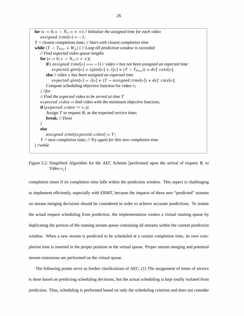
Figure 3.2 shows a simplified algorithm of AEC. This algorithm is performed uponthe arrival of

requestRi to videov j when the server is fully loaded. If the server is not fully loaded, the request can

be serviced immediately. The assigned time for videov (assignedtime[v]) corresponds to the latest

completion time (Tl ) at which videov is expected to be serviced in Equation (3.2).

Figure 3.3 demonstrates the general idea of AEC. A new request for video 2 (v2) arrives at time

TNow. The server finds that video 1 (v1) is the expected video to be serviced at stream completion time

T1. Then, the server examines the next completion timeT2 (which is still within the prediction window)

and determines thatv2 is the most likely to be serviced at that time. Becausev2 is the requested video

for which we need to find the expected time of service, the prediction algorithmterminates by assigning

T2 as the expected time of service to the new request.

The proposed AEC algorithm involves another important aspect:prediction of stream completion

times. The server here uses aggressive prediction. It not only predicts how the completion times will

be assigned to incoming requests but also predicts new stream completion times and assigns them if

possible to new requests. When AEC assigns a stream completion time to a request as the expected

time of service, it adds the expected completion time of the new stream to the set ofthe to-be examined

26

for (v = 0; v < Nv ; v + +) // Initialize the assigned time for each videoassignedtime[v] = −1;

T = closest completion time;// Start with closest completion timewhile (T < TNow + Wp) { // Loop till prediction window is exceeded

// Find expected video queue lengthsfor (v = 0; v < Nv ; v + +){

if ( assignedtime[v] == −1) // video v has not been assigned an expected timeexpectedqlen[v] = (qlen[v] + λ[v] × (T − TNow)) × def rate[v];

else// videov has been assigned an expected timeexpectedqlen[v] = λ[v] × (T − assignedtime[v]) × def rate[v];

Compute scheduling objective function for videov;} //for// Find the expected video to be served at time Texpectedv ideo= find video with the minimum objective function;if (expectedv ideo== v j ){

AssignT to requestRi as the expected service time;break; // Done

}

elseassignedtime[expectedv ideo] = T ;

T = next completion time;// Try again for this new completion time} //while

Figure 3.2: Simplified Algorithm for the AEC Scheme [performed upon the arrival of requestRi toVideo v j ]

completion times if its completion time falls within the prediction window. This aspect is challenging

to implement efficiently, especially with ERMT, because the impacts of these new “predicted” streams

on stream merging decisions should be considered in order to achieve accurate predictions. To isolate

the actual request scheduling from prediction, the implementation creates a virtual running queue by

duplicating the portion of the running stream queue containing all streams withinthe current prediction

window. When a new stream is predicted to be scheduled at a certain completion time, its own com-

pletion time is inserted in the proper position in the virtual queue. Proper streammerging and potential

stream extensions are performed on the virtual queue.

The following points serve as further clarifications of AEC. (1) The assignment of times of service

is done based on predicting scheduling decisions, but the actual scheduling is kept totally isolated from

prediction. Thus, scheduling is performed based on only the scheduling criterion and does not consider

27

(a) Assignment of Completion Time T1

(b) Assignment of Completion Time T2

Figure 3.3: Clarification of the AEC Scheme

the assigned expected times of service in any way. (2) AEC may assign the same expected time to

requests for different videos because the assignments are based on the current server state and workload,

which vary with time. Similarly, the requests for the same video that are currentlytogether in the waiting

queue may have received different expected waiting times although they willbe serviced together. Later

requests in the queue are more likely to receive more accurate predictions.(3) Because of the prediction

window constraint, AEC may not give an expected time for each user. As willbe discussed in Subsection

3.3.4, the proposed hybrid scheme addresses this limitation.

3.3.2 Proposed Enhancements of AEC

We propose the following two enhancements of AEC:Preferential Treatment of Real Requestsand

Refine Assigned Expected Times.

28

Preferential Treatment of Real Requests

With AEC, the expected queue lengths are computed and used to predict future scheduling decisions.

An expected queue length includes a number of real requests and a number of expected requests. This

enhancement values real requests more than expected requests. One interesting way to implement this

enhancement is to truncate the expected queue lengths in Equations (3.1) and (3.2). Thus, if a video has

an expected queue length less than one, it will not be selected as an expected video to be serviced at any

stream completion time.

Periodic Refinement of Assigned Expected Times

With this enhancement, the server periodically attempts to provide users with updated expected times

of service. For a waiting request already assigned an expected time of service, a new time of service

becomes available whenever a new request for the same video arrives and receives an expected time

because all requests for the same video will be serviced concurrently using only one stream. The new

expected time will most likely be more accurate than the old one because it is estimated based on the

latest system state. To avoid unnecessary updates, this enhancement provides updated expected times

only when a considerable difference exists between the new and old expected times. With the periodic

refinement, some requests that never received expected times before maybe able to get expected times

later on as updates. Therefore, this enhancement is expected to improve both the prediction accuracy

and the percentage of users receiving expected times. Unless otherwiseindicated, the reported accuracy

is determined based on the deviation of the initial expected service time and the actual time of service.

3.3.3 Feedback Control of the Prediction Window

In addition to limiting the implementation complexity, the prediction window introduces a tradeoff

between the percentage of requests receiving expected times of serviceand the prediction accuracy. In

particular, as the prediction window increases, the number of requests receiving expected times increases

29

at the expense of reducing the prediction accuracy as well as increasing the implementation complexity.

The AEC algorithm computation time is proportional to the prediction window and can be shown to be

O(Nv × Wp), whereNv is the number of videos. Subsection 3.5.4 analyzes the impact of the prediction

window based on actual runs of the algorithm. Large prediction windows have negative impacts on

the algorithm computation time and more importantly the prediction accuracy. The reduced prediction

accuracy may have a serious impact on the user-perceived quality of service and the confidence of users

in the provided expected waiting times. The prediction window in AEC is constrained because the

proposed AEC algorithm does not predict the waiting times accurately beyond a certain value of the

prediction window, and it is better to provide no prediction than to provide misleading or inaccurate

waiting times.

We utilize feedback control theory to tuneWp to allow a pre-specified tolerance in the accuracy.

Here, the administrator sets the minimum value of accuracy that can be tolerated. This value, called

setpoint, can be specified in the form of the tolerable average deviation between theactual and expected

times of service. Ideally,Wp should be set to the largest possible value that satisfies the setpoint in

order to maximize the number of users receiving expected times. The loop control is driven by theerror

(e(t)), which is the difference between the setpoint and the actual average deviation (called theprocess

variable).

For stable and accurate control, we use aProportional Integral Differential(PID), as depicted in

Figure 3.4(a), to adjustWp based on the history and rate of change of the error. It has three components:

proportional, integral, and differential. Each component is weighted by a constant. The proportional

component changesWp based on the immediate value of the error. The integral component considers

the past values of the error, whereas the differential component anticipates the future, and thus they help

reduce the steady state error and the overshoot, respectively.

To eliminate the problem of optimizing three constants in the PID Controller, we propose another

controller, calledExponential Controller, which uses the power of the error, as shown in Figure 3.4(b).

30

The power of the error is used because when the error is small,Wp should be changed slightly to

minimize overshooting and undershooting. When the error however, is large, Wp should be changed by

large values to expedite the convergence to the desired setpoint. By extensive analysis, we found that

the best function issign(e(t)) × 2|e(t)|.

(a) PID Controller

(b) Proposed Exponential Controller

Figure 3.4: Controllers of Prediction Accuracy

3.3.4 Proposed Hybrid Prediction Scheme

The main problem with the AEC scheme is that not all users may receive an expected time of service.

To address this problem, we propose and analyze an alternative scheme,calledHybrid Prediction, which

can give an expected time to each user. The hybrid scheme first uses AECto predict the waiting time,

and if no prediction is made, it provides the user with the average per-videowaiting time. Thus, it can

be thought of as a hybrid of AEC and APW. The use of APW enables the hybrid scheme to provide

a predicted waiting times for each request at the expense of lower prediction accuracy. The prediction

windows has an important impact on the accuracy of this hybrid predictor. As the prediction window

increases, a larger fraction of users will receive expected times using AEC, which is more accurate than

APW for small values of the prediction window.

31

3.4 Evaluation Methodology

We analyze the effectiveness of the proposed schemes through extensive simulation.

3.4.1 Workload Characteristics

Table 5.2 summarizes the workload characteristics used. Like most prior studies, we generally

assume that the arrival of the requests to the server follows a Poisson Process with an average arrival

rateλ. We also experiment with the Weibull distribution with two parameters: shape andscale [67] . We

analyze the impact of the shape (k), while adjusting the scale so that the desired average request arrival

rate is reached. Additionally, we assume that the access to videos is highly localized and follows a Zipf-

like distribution. With this distribution, the probability of choosing thenth most popular video isC/n1−θ

with a parameterθ and a normalized constantC. The parameterθ controls the skew of video access.

Note that the skew reaches its peak whenθ = 0, and that the access becomes uniformly distributed when

θ = 1. We analyze the impact of this parameter, but we generally assume a value of 0.271 [66, 65].

We characterize the waiting tolerance of users by three models. InModel A, the waiting tolerance

follows an exponential distribution with meanµtol [66, 65]. In Model B, users with expected waiting

times less thanµtol will wait, and the others exhibit the same waiting tolerance as Model A [66, 65].

We introduceModel Cto capture situations in which users either wait or defect immediately depending

on the expected waiting times. The user waits if the expected waiting time is less thanµtol and defects

immediately if the waiting time is greater than 2µtol . Otherwise, the defection probability increases

linearly from 0 to 1 for the expected waiting times betweenµtol and 2µtol . In all these models, defections

happen only while users are waiting for service.

We generally study a server with 120 videos, each of which is 120 minutes long. We examine the

server at different loads by fixing the request arrival rate at 40 requests per minute and varying the

number of channels (server capacity) generally from 300 to 750. In addition to the fixed-length video

workload (in which all videos have the same length), we experiment with two variable-length video

32

workloads. Moreover, we study the impacts of arrival rate, user’s waiting tolerance, number of videos,

and video length (in the fixed-length workload).

Table 3.1: Summary of Workload CharacteristicsParameter Model/Value(s)Request Arrival Poisson Process (Default)

Weibull Distribution with shapek = 0.6 to 0.9Request Arrival Rate (λ) 10 to 70 Requests/min, Default = 40 Requests/minServer Capacity 300 to 750 channelsVideo Access Zipf-LikeVideo Skew (θ) 0.1 to 0.6, Default = 0.271Number of Videos 60 to 240, Default = 120Video Length Fixed-Length Video Workload (Default)

with length of 30 to 120 min (same for all videos),Default = 120 min

Variable-Length Video Workload 1:with lengths randomly in the range: 30 to 120 min

Variable-Length Video Workload 2:with lengths randomly in the range: 100 to 200 min

Waiting Tolerance Model A, B, and CWaiting Tolerance Mean (µtol) 15 to 90 sec, Default = 30 sec

3.4.2 Performance Metrics

We use two performance metrics to compare the effectiveness of various prediction schemes:waiting-

time prediction accuracyandpercentage of clients receiving expected times of service(PCRE). Theav-

erage deviationbetween the expected and actual times of service is used as a measure of accuracy. The

accuracy decreases with the deviation.

We compare the effectiveness of the predictive and GNSTF approaches in terms of the user defection

probability, average waiting time, and unfairness against unpopular videos.

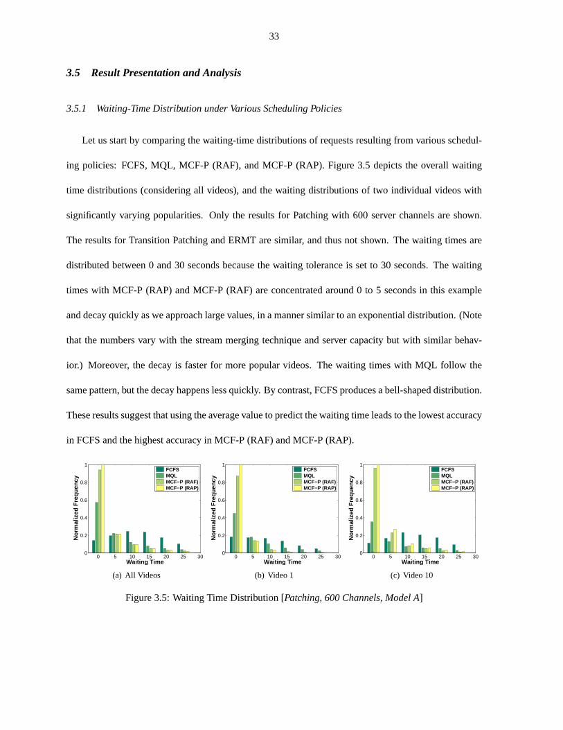
33

3.5 Result Presentation and Analysis

3.5.1 Waiting-Time Distribution under Various Scheduling Policies

Let us start by comparing the waiting-time distributions of requests resulting from various schedul-

ing policies: FCFS, MQL, MCF-P (RAF), and MCF-P (RAP). Figure 3.5 depicts the overall waiting

time distributions (considering all videos), and the waiting distributions of two individual videos with

significantly varying popularities. Only the results for Patching with 600 server channels are shown.

The results for Transition Patching and ERMT are similar, and thus not shown. The waiting times are

distributed between 0 and 30 seconds because the waiting tolerance is set to30 seconds. The waiting

times with MCF-P (RAP) and MCF-P (RAF) are concentrated around 0 to 5 seconds in this example

and decay quickly as we approach large values, in a manner similar to an exponential distribution. (Note

that the numbers vary with the stream merging technique and server capacitybut with similar behav-

ior.) Moreover, the decay is faster for more popular videos. The waiting times with MQL follow the

same pattern, but the decay happens less quickly. By contrast, FCFS produces a bell-shaped distribution.

These results suggest that using the average value to predict the waiting timeleads to the lowest accuracy

in FCFS and the highest accuracy in MCF-P (RAF) and MCF-P (RAP).

0 5 10 15 20 25 300

0.2

0.4

0.6

0.8

1

Nor

mal

ized

Fre

quen

cy

Waiting Time

FCFS MQL MCF−P (RAF) MCF−P (RAP)

(a) All Videos

0 5 10 15 20 25 300

0.2

0.4

0.6

0.8

1

Nor

mal

ized

Fre

quen

cy

Waiting Time


(b) Video 1

0 5 10 15 20 25 300

0.2

0.4

0.6

0.8

1

Nor

mal

ized

Fre

quen

cy

Waiting Time


(c) Video 10

Figure 3.5: Waiting Time Distribution [Patching, 600 Channels, Model A]

34

3.5.2 Waiting-Time Predictability and Effectiveness of Various Prediction Schemes

Let us now compare the effectiveness of the proposed prediction schemes in terms of accuracy,

which is the most important metric in this case. Figures 3.6, 3.7, and 3.8 depict theaverage deviation

results for ERMT, Transition Patching, and Patching under three different scheduling policies: MQL,

MCF-P (RAF), and MCF-P (RAP). (FCFS, in the form of NSTF/GNSTF, ismore suited for providing

hard time-of-service guarantees than prediction. Subsection 3.5.8 analyzes the performance of GNSTF.)

These figures demonstrate that AEC performs significantly better than APW and the results are better

with more scalable stream merging. The deviation with AEC is within only two seconds. APW has the

advantage of giving an expected time of service to each user, but the accuracy of these expectations is a

more important factor. The hybrid scheme serves as a compromise between AEC and APW.

The two variants of MCF-P (RAF and RAP) perform very close to each other in accuracy. MCF-

P, however, is more predictable than MQL because the scheduling decisions of MCF-P are based on

both the queue lengths and the required stream costs, whereas MQL usesonly the queue lengths. The

required stream cost for a video can be determined precisely, but the queue lengths in the future require

prediction, as done in Equations (3.1) and (3.2). Fortunately, MCF-P is not only more predictable than

MQL but also achieves better performance (as shown in [22]) in terms of defection probability, average

waiting time, and unfairness. From this point on, we consider only MCF-P (RAP) and refer to it simply

as MCF-P.

300 400 500 600 7000

2

4

6

8

10

12

14

Ave

rage

Dev

iatio

n (s

econ

ds)

Server Capacity

APW AEC Hybrid

(a) ERMT

300 400 500 600 7000

5

10

15

Ave

rage

Dev

iatio

n (s

econ

ds)

Server Capacity

APW AEC Hybrid

(b) Transition Patching

300 400 500 600 7004

6

8

10

12

14

16

Ave

rage

Dev

iatio

n (s

econ

ds)

Server Capacity

APW AEC Hybrid

(c) Patching

Figure 3.6: Comparing the Accuracy of Prediction Schemes [MQL, Wp = 0.5µtol , Model A]

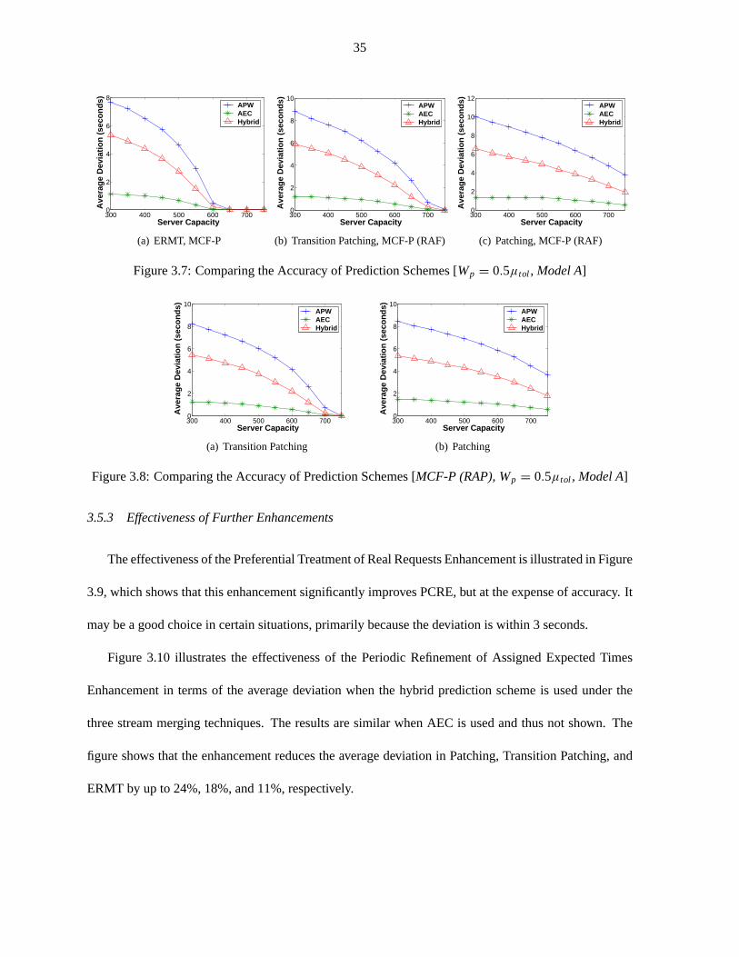
35

300 400 500 600 7000

2

4

6

8 A

vera

ge D

evia

tion

(sec

onds

)

Server Capacity

APW AEC Hybrid

(a) ERMT, MCF-P

300 400 500 600 7000

2

4

6

8

10

Ave

rage

Dev

iatio

n (s

econ

ds)

Server Capacity

APW AEC Hybrid

(b) Transition Patching, MCF-P (RAF)

300 400 500 600 7000

2

4

6

8

10

12

Ave

rage

Dev

iatio

n (s

econ

ds)

Server Capacity

APW AEC Hybrid

(c) Patching, MCF-P (RAF)

Figure 3.7: Comparing the Accuracy of Prediction Schemes [Wp = 0.5µtol , Model A]

300 400 500 600 7000

2

4

6

8

10

Ave

rage

Dev

iatio

n (s

econ

ds)

Server Capacity

APW AEC Hybrid

(a) Transition Patching

300 400 500 600 7000

2

4

6

8

10

Ave

rage

Dev

iatio

n (s

econ

ds)

Server Capacity

APW AEC Hybrid

(b) Patching

Figure 3.8: Comparing the Accuracy of Prediction Schemes [MCF-P (RAP), Wp = 0.5µtol , Model A]

3.5.3 Effectiveness of Further Enhancements

The effectiveness of the Preferential Treatment of Real Requests Enhancement is illustrated in Figure

3.9, which shows that this enhancement significantly improves PCRE, but atthe expense of accuracy. It

may be a good choice in certain situations, primarily because the deviation is within3 seconds.

Figure 3.10 illustrates the effectiveness of the Periodic Refinement of Assigned Expected Times

Enhancement in terms of the average deviation when the hybrid prediction scheme is used under the

three stream merging techniques. The results are similar when AEC is used and thus not shown. The

figure shows that the enhancement reduces the average deviation in Patching, Transition Patching, and

ERMT by up to 24%, 18%, and 11%, respectively.

36

300 350 400 450 500 550 6000

0.5

1

1.5

2

2.5

3

3.5

Ave

rage

Dev

iatio

n (s

econ

ds)

Server Capacity

without Enhanement with Enhancement

(a) Deviation

300 350 400 450 500 550 6000

20

40

60

80

100

% C

lient

s W

ith E

xpec

ted

Tim

es

Server Capacity

without Enhanement with Enhancement

(b) PCRE

Figure 3.9: Effectiveness of the Preferential Treatment of Real Requests Enhancement [ERMT, MCF-P,AEC, Wp = µtol , Model A]

300 400 500 600 7000

1

2

3

4

5

6

Ave

rage

Dev

iatio

n (s

econ

ds)

Server Capacity

without Enhamcement with Enhamcement

(a) ERMT, MCF-P

300 400 500 600 7000

1

2

3

4

5

6

Ave

rage

Dev

iatio

n (s

econ

ds)

Server Capacity


(b) Transition Patching, MCF-P (RAP)

300 400 500 600 7001

2

3

4

5

6

Ave

rage

Dev

iatio

n (s

econ

ds)

Server Capacity


(c) Patching, MCF-P (RAP)

Figure 3.10: Impact of the Periodic Refinement of Assigned Expected TimesEnhancement on the Hy-brid Prediction Scheme [Wp = µtol , Model A]

3.5.4 Impact of Prediction Window

Figure 3.11(a) plots the impact of prediction window (Wp) in AEC on the prediction accuracy and

PCRE for the three stream merging techniques. As expected, both the deviation and PCRE increase with

Wp. PCRE significantly increases withWp up to a certain point, after which it starts to increase slightly.

Both these metrics generally improve with more scalable stream merging, exceptfor large values of

Wp. When the Preferential Treatment of Real Requests Enhancement is used, a significantly different

behavior is observed, especially in the deviation, as shown in Figure 3.11(b). The deviation increases

with Wp up to a certain point, after which it reaches a steady value. The impact ofWp in the case of the

hybrid prediction scheme is shown in Figure 3.11(c). The accuracy increases withWp up to a certain

value and then starts to decrease. (Recall that the accuracy decreases with the deviation.) The increase

37

is due to increasing the fraction of clients receiving expected times by AEC (which is more accurate)

rather than APW. After a certain value, the reduced accuracy of AEC withWp becomes more dominant.

0 20 40 60 80 100 1200

1

2

3

4

5

6

7

8

Ave

rage

Dev

iatio

n (s

econ

ds)

Prediction Window (seconds)

MCF−P (RAP) with Patching MCF−P (RAP) with Transition Patching MCF−P with ERMT

0 20 40 60 80 100 1200

10

20

30

40

50

60

70

80

% o

f Clie

nts

with

Exp

ecte

d T

imes



(a) AEC without Enhancement

0 20 40 60 80 100 1200

0.5

1

1.5

2

2.5

3

3.5

Ave

rage

Dev

iatio

n (s

econ

ds)



(b) AEC with Enhancement

0 20 40 60 80 100 120

3

4

5

6

7

8

Ave

rage

Dev

iatio

n (s

econ

ds)


MCF−P (RAP) + Hybrid with Patching MCF−P (RAP) + Hybrid with Transition Patching MCF−P + Hybrid with ERMT

(c) Hybrid without Enhancement

Figure 3.11: Impact of Prediction Window without and with the Preferential Treatment of Real RequestsEnhancement [MCF-P, 500 Channels, Model A]

Figure 3.12 demonstrates the impact of the prediction window on the average computation time

of the AEC algorithm. The results are obtained by averaging the computation time values during the

entire lifetime of the simulation. The figure illustrates the increased implementation complexity with

the prediction window and indicates a linear relationship.

0 20 40 600

0.2

0.4

0.6

0.8

1

Nor

mal

ized

Ave

rage

Tim

e


MCF−P (RAP) with Patching MCF−P with ERMT

Figure 3.12: Impact of Prediction Window on Algorithm Computation Time [AEC, 500 Channels,Model A]

38

3.5.5 Analysis of Deviation Distributions under Various Prediction Schemes

So far, we compared various prediction schemes in only the average deviation. In this subsection, we

discuss the distributions of the deviation results, so that we can compare various schemes in the range,

standard deviation (σ ), and confidence interval (C I ). Figure 3.13 shows the distributions of the deviation

for the three prediction schemes. The results for AEC and Hybrid are shown for two and three values

of the prediction window, respectively. Table 3.2 shows the means, standard deviations, and the 90%

confidence intervals for various schemes. As expected, AEC providesthe smallest standard deviation,

and the shortest confidence interval, and these values increase with the prediction window. Although

the hybrid scheme performs better than APW in the average accuracy (as shown in Subsection 3.5.2),

it provides comparable results to APW in terms of the standard deviation and theconfidence interval.

Note that the means of the distribution can be positive or negative. A negative value indicates a stronger

negative deviation component, whereas a positive value indicates a stronger positive deviation compo-

nent. A negative deviation means that a user waits shorter than expected, while a positive deviation

means waiting longer than expected. It is possible to assign different weights for negative and positive

deviations, but in this study we treat them equally. Accurate waiting times help users wait accordingly,

so it may not be beneficial if the user waits less than expected because the user may be doing something

else meanwhile. Finally, it is useful to study the relative deviation compared to the actual waiting time.

Figure 3.14 compares the distributions of the deviation percentage of the three prediction algorithms.

These results illustrate that the benefits of AEC, especially compared to APW,are more outstanding in

terms the percentage deviation.

3.5.6 Impact of Workload Parameters on AEC Performance

Figures 3.15 and 3.16 show the impacts of request arrival rate, user’swaiting tolerance, skew in

video access (θ), number of videos, and video length on the effectiveness of AEC in termsof accuracy

and PCRE, respectively. The deviation increases with the arrival rate but remains with 2 seconds even

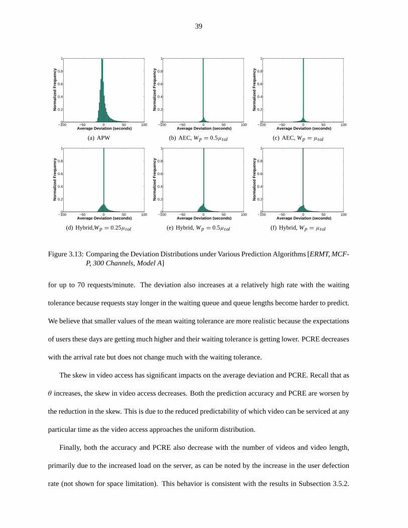
39

−100 −50 0 50 1000

0.2

0.4

0.6

0.8

1

Average Deviation (seconds)

Nor

mal

ized

Fre

quen

cy

(a) APW

−100 −50 0 50 1000

0.2

0.4

0.6

0.8

1


Nor

mal

ized

Fre

quen

cy

(b) AEC,Wp = 0.5µtol

−100 −50 0 50 1000

0.2

0.4

0.6

0.8

1


Nor

mal

ized

Fre

quen

cy

(c) AEC,Wp = µtol

−100 −50 0 50 1000

0.2

0.4

0.6

0.8

1


Nor

mal

ized

Fre

quen

cy

(d) Hybrid,Wp = 0.25µtol

−100 −50 0 50 1000

0.2

0.4

0.6

0.8

1


Nor

mal

ized

Fre

quen

cy

(e) Hybrid,Wp = 0.5µtol

−100 −50 0 50 1000

0.2

0.4

0.6

0.8

1


Nor

mal

ized

Fre

quen

cy

(f) Hybrid, Wp = µtol

Figure 3.13: Comparing the Deviation Distributions under Various Prediction Algorithms [ERMT, MCF-P, 300 Channels, Model A]

for up to 70 requests/minute. The deviation also increases at a relatively high rate with the waiting

tolerance because requests stay longer in the waiting queue and queue lengths become harder to predict.

We believe that smaller values of the mean waiting tolerance are more realistic because the expectations

of users these days are getting much higher and their waiting tolerance is getting lower. PCRE decreases

with the arrival rate but does not change much with the waiting tolerance.

The skew in video access has significant impacts on the average deviation and PCRE. Recall that as

θ increases, the skew in video access decreases. Both the prediction accuracy and PCRE are worsen by

the reduction in the skew. This is due to the reduced predictability of which video can be serviced at any

particular time as the video access approaches the uniform distribution.

Finally, both the accuracy and PCRE also decrease with the number of videos and video length,

primarily due to the increased load on the server, as can be noted by the increase in the user defection

rate (not shown for space limitation). This behavior is consistent with the results in Subsection 3.5.2.

40

Table 3.2: Summary of Deviation Distributions [ERMT, MCF-P, 300 Channels, Model A]Scheme Mean (sec) Standard Deviation (sec) 90%Confidence Interval (sec)APW -0.027 12.5604 [-14.0396,14.0104]AEC, Wp = 0.25µtol 0.4537 2.6762 [-1.5707,2.4793]AEC, Wp = 0.5µtol 0.2367 3.3914 [-3.8063,4.2437]AEC, Wp = µtol -0.6131 5.2066 [-7.8732,6.6768]Hybrid, Wp = 0.25µtol 2.4055 11.7448 [-11.7366,16.5134]Hybrid, Wp = 0.5µtol 2.0781 11.6507 [-11.8441,16.0059]Hybrid, Wp = µtol 1.3027 11.8306 [-13.5439,16.1061]

−5 0 5 10 15 20 250

0.2

0.4

0.6

0.8

1

Deviation Percentage

Nor

mal

ized

Fre

quen

cy

(a) APW

−5 0 5 10 15 20 250

0.2

0.4

0.6

0.8

1


Nor

mal

ized

Fre

quen

cy

(b) AEC

−5 0 5 10 15 20 250

0.2

0.4

0.6

0.8

1


Nor

mal

ized

Fre

quen

cy

(c) Hybrid

Figure 3.14: Comparing the Distributions of the Deviation Percentage [ERMT, MCF-P, Wp = 0.5µtol ,300 Channels, Model A]

The increase in the server load as the number of videos increases happens as a result of the reduction

in data sharing. Although the deviation increases with the number of videos, itremains with 2 seconds

even for up to 240 supported videos.

The results so far are for a video workload of a fixed video length. Figure 3.17 shows the average

deviation and PCRE results for two different variable-length workloads.The first is comprised of videos

with lengths in the range of 30 to 120 minutes, whereas the lengths in the secondrange from 100 to

200 minutes. The length of each video is generated randomly within the specified range. The results for

each workload are obtained by averaging the values of three runs. TheAEC algorithm also works well in

these workloads, with an average deviation within only 2.5 seconds. For workloads with longer videos,

the server load becomes larger (as indicated in Figure 3.17(c)), and thusboth the average deviation and

PCRE become worse.

41

10 20 30 40 60 700

0.5

1

1.5

2

2.5 A

vera

ge D

evia

tion

(sec

onds

)

Arrival Rate (client/min)


(a) Impact of Arrival Rate

15 30 45 60 75 900

1

2

3

4

5

6

Ave

rage

Dev

iatio

n (s

econ

ds)

Waiting Tolerance Mean (seconds)


(b) Impact of Waiting Tolerance

0.1 0.2 0.3 0.4 0.5 0.60.5

1

1.5

2

2.5

Ave

rage

Dev

iatio

n (s

econ

ds)

Skew Parameter ( θ)


(c) Impact of Skew in Video Access

60 90 120 150 180 210 2400

0.5

1

1.5

2

2.5

Ave

rage

Dev

iatio

n (s

econ

ds)

Number of Videos


(d) Impact of Number of Videos

30 45 60 75 90 105 1200

0.5

1

1.5

2

Ave

rage

Dev

iatio

n (s

econ

ds)

Video Length (min)


(e) Impact of Video Length

Figure 3.15: Impact of Workload on Average Deviation [AEC, 550 Channels, Wp = µtol , Model A]

The results so far assume a Poisson request arrival process. Let us now examine the behavior under

Weibull distribution with different shape (k) values. Figure 3.18 demonstrates that the waiting times can

still be predicted accurately with the AEC algorithm. The shape has a little impact, especially when the

prediction window is smaller than 35 seconds.

3.5.7 Feedback Control of the Prediction Window in AEC

Let us now discuss the effectiveness of using the proposed controllerof the prediction window, when

the AEC scheme is used. Figure 3.19 demonstrates how the PID Controller caneffectively achieve five

desired accuracy values (setpoints): 0.5, 1.5, 2.5, 3.5, and 4.5 seconds with different stream merging

techniques. By dynamically tuningWp to the largest possible value that satisfies the setpoint, the PID

Controller ensures the largest possible value of PCRE. As the tolerable accuracy increases from 0.5 to

4.5, PCRE increases by more than 39%, 46%, and 93% with ERMT, Transition Patching, and Patching

respectively. The system administrator should consider this significant implication of the setpoint on

PCRE. Figure 3.20 shows how that the Exponential Controller behaves close to the PID Controller. The

42

10 20 30 40 60 70

40

50

60

70

80

90

100 %

of C

lient

s W

ith E

xpec

ted

Tim

e

Arrival Rate (client/min)


(a) Impact of Arrival Rate

15 30 45 60 75 9055

60

65

70

75

80

85

90

% o

f Clie

nts

With

Exp

ecte

d T

ime

Waiting Tolerance Mean (seconds)


(b) Impact of Waiting Tolerance

0.1 0.2 0.3 0.4 0.5 0.60.5

0.55

0.6

0.65

0.7

0.75

0.8

0.85

% o

f Use

rs W

ith E

xpec

ted

Tim

es



(c) Impact of Skew in Video Access

60 90 120 150 180 210 240

30

40

50

60

70

80

90

100

% o

f Clie

nts

With

Exp

ecte

d T

ime

Number of Videos


(d) Impact of Number of Videos

30 45 60 75 90 105 12050

60

70

80

90

100

% o

f Clie

nts

With

Exp

ecte

d T

ime

Video Length (min)


(e) Impact of Video Length

Figure 3.16: Impact of Workload on PCRE [AEC, 550 Channels, Wp = µtol , Model A]

PID Controller has a little advantage over the Exponential for small setpoints,where it achieves larger

PCRE because it has a slightly larger overshoot and is a little faster in reaching the desired setpoint.

3.5.8 Effectiveness of the Waiting-Time Prediction Approach Compared with GNSTF

As discussed earlier, GNSTF is a scheduling policy that performs request scheduling based on the

schedule times, which are initially assigned on a FCFS basis. The proposed waiting-time prediction

approach allows the application of aggressive cost-based scheduling policies and hierarchical stream

merging techniques (such as MCF-P and ERMT, respectively). In this subsection, we demonstrate

the implications of the predictive approach on improving system performance interms of the overall

user defection rate and average waiting time. The prediction approach here is applied with MCF-P

and this combination is referred to as “Predictive MCF-P”. Figures 3.21 and 3.22 compare the two

approaches in user defection probability, average waiting time, and unfairness for Model B and C of the

waiting tolerance, respectively. Three variants of Predictive MCF-P are analyzed. The first two apply

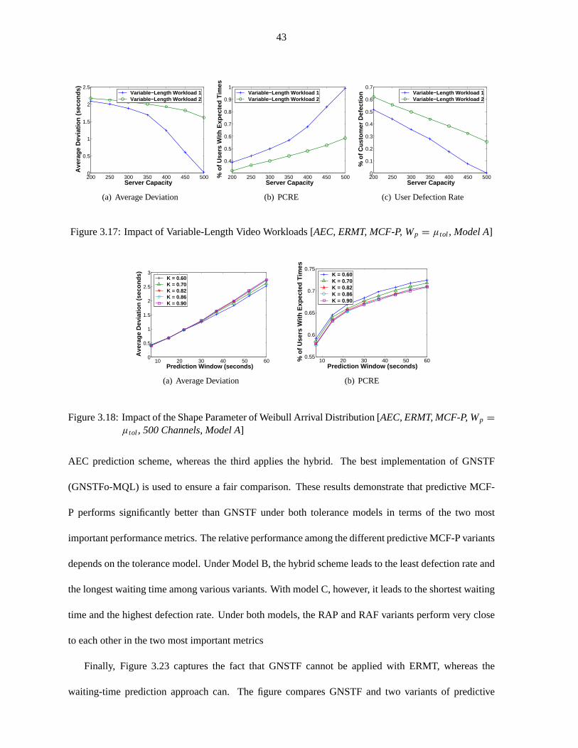
43

200 250 300 350 400 450 5000

0.5

1

1.5

2

2.5

Ave

rage

Dev

iatio

n (s

econ

ds)

Server Capacity

Variable−Length Workload 1 Variable−Length Workload 2

(a) Average Deviation

200 250 300 350 400 450 500

0.4

0.5

0.6

0.7

0.8

0.9

1

% o

f Use

rs W

ith E

xpec

ted

Tim

es

Server Capacity


(b) PCRE

200 250 300 350 400 450 5000

0.1

0.2

0.3

0.4

0.5

0.6

0.7

% o

f Cus

tom

er D

efec

tion

Server Capacity


(c) User Defection Rate

Figure 3.17: Impact of Variable-Length Video Workloads [AEC, ERMT, MCF-P, Wp = µtol , Model A]

10 20 30 40 50 600

0.5

1

1.5

2

2.5

3

Ave

rage

Dev

iatio

n (s

econ

ds)


K = 0.60 K = 0.70 K = 0.82 K = 0.86 K = 0.90


10 20 30 40 50 600.55

0.6

0.65

0.7

0.75

% o

f Use

rs W

ith E

xpec

ted

Tim

es


K = 0.60 K = 0.70 K = 0.82 K = 0.86 K = 0.90

(b) PCRE

Figure 3.18: Impact of the Shape Parameter of Weibull Arrival Distribution[AEC, ERMT, MCF-P, Wp =

µtol , 500 Channels, Model A]

AEC prediction scheme, whereas the third applies the hybrid. The best implementation of GNSTF

(GNSTFo-MQL) is used to ensure a fair comparison. These results demonstrate that predictive MCF-

P performs significantly better than GNSTF under both tolerance models in termsof the two most

important performance metrics. The relative performance among the different predictive MCF-P variants

depends on the tolerance model. Under Model B, the hybrid scheme leads tothe least defection rate and

the longest waiting time among various variants. With model C, however, it leadsto the shortest waiting

time and the highest defection rate. Under both models, the RAP and RAF variants perform very close

to each other in the two most important metrics

Finally, Figure 3.23 captures the fact that GNSTF cannot be applied with ERMT, whereas the

waiting-time prediction approach can. The figure compares GNSTF and two variants of predictive

44

0 2 4 6 8

x 106

00.5

2.5

4.5

6.5

8.5

10.5 A

vera

ge D

evia

tion

(sec

onds

)

Time (seconds)

Setpoint = 0.5, PCRE = 46%





(a) ERMT, MCF-P, 450 Channels

0 2 4 6 8

x 106

00.5

2.5

4.5

6.5

8.5

10.5

Ave

rage

Dev

iatio

n (s

econ

ds)

Time (seconds)






(b) Transition Patching, MCF-P (RAP),500 Channels

0 2 4 6 8

x 106

00.5

2.5

4.5

6.5

8.5

10.5

Ave

rage

Dev

iatio

n (s

econ

ds)

Time (seconds)






(c) Patching, MCF-P (RAP), 550 Chan-nels

Figure 3.19: Effectiveness of PID Controller using different Average Deviation Setpoints [AEC, ModelA, Kp = 7, K i = 1, Kd = 0.1]

0 2 4 6 8

x 106

00.5

2.5

4.5

6.5

8.5

10.5

Ave

rage

Dev

iatio

n (s

econ

ds)

Time (seconds)






(a) ERMT, MCF-P, 450 Channels

0 2 4 6 8

x 106

00.5

2.5

4.5

6.5

8.5

10.5

Ave

rage

Dev

iatio

n (s

econ

ds)

Time (seconds)






(b) Transition Patching, MCF-P (RAP),500 Channels

0 2 4 6 8

x 106

00.5

2.5

4.5

6.5

8.5

10.5

Ave

rage

Dev

iatio

n (s

econ

ds)

Time (seconds)

Setpoint = 0.5 PCRE = 26%





(c) Patching, MCF-P (RAP), 550 Chan-nels

Figure 3.20: Effectiveness of Exponential Controller using differentAverage Deviation Setpoints [AEC,Model A]

MCF-P (AEC and Hybrid), when each is applied with the most scalable streammerging technique that

is applicable to it. Here, only the results under Model C (which is more realistic)are shown. Model

B exhibits a similar behavior. The results demonstrate the outstanding performance gains achieved by

applying the prediction approach in terms of the two most important performance metrics. The two

variants perform generally close to each other.

3.6 Conclusions

We have analyzed the waiting-time predictability in scalable video streaming and have presented

two prediction schemes:Assign Expected Stream Completion Time(AEC) andHybrid Prediction. AEC

utilizes detailed information about the server state and considers the applied scheduling policy to predict

45

300 400 500 600 7000

20

40

60

80 %

of C

usto

mer

Def

ectio

n

Server Capacity

GNSTF MCF−P (RAF) + AEC MCF−P (RAP) + AEC MCF−P (RAP) + Hybrid

(a) Defection Rate

300 400 500 600 7000

5

10

15

20

25

30

35

Ave

rage

Wai

ting

Tim

e (s

econ

ds)

Server Capacity


(b) Waiting Time

300 400 500 600 7000

0.01

0.02

0.03

0.04

Unf

airn

ess

Server Capacity


(c) Unfairness

Figure 3.21: Comparing GNSTF with Predictive MCF-P (Three Variants) [Transition Patching, Wp =

0.5µtol , Model B]

300 400 500 600 7000

20

40

60

80

% o

f Cus

tom

er D

efec

tion

Server Capacity


(a) Defection Rate

300 400 500 600 7000

5

10

15

20

25

Ave

rage

Wai

ting

Tim

e (s

econ

ds)

Server Capacity


(b) Waiting Time

300 400 500 600 7000

0.005

0.01

0.015

0.02

0.025

Unf

airn

ess

Server Capacity


(c) Unfairness

Figure 3.22: Comparing GNSTF with Predictive MCF-P (Three Variants) [Transition Patching, Wp =

0.5µtol , Model C]

the future scheduling decisions over a certain period, calledprediction window. This window introduces

a tradeoff between the prediction accuracy and the number of users receiving expected waiting times.

The hybrid scheme uses AEC and then assigns the average video waiting time for those requests that did

not obtain a predicted time by AEC.

We have analyzed the effectiveness of the two prediction schemes when applied with various stream

merging techniques and scheduling policies. We have also compared the effectiveness of the waiting-

time prediction approach with the approach that provides time-of-service guarantees. The latter is rep-

resented by an extended policy, calledGeneralized Next Schedule Time First(GNSTF). In addition, we

have studied the impacts of prediction window, server capacity, user’s waiting tolerance, arrival rate,

skew in video access, video length, and number of videos.

The main results can be summarized as follows.

46

300 400 500 600 7000

20

40

60

80 %

of C

usto

mer

Def

ectio

n

Server Capacity

GNSTF with Transition Patching MCF−P + AEC with ERMT MCF−P + Hybrid with ERMT

(a) Defection Rate

300 400 500 600 7000

5

10

15

20

25

30

Ave

rage

Wai

ting

Tim

e (s

econ

ds)

Server Capacity


(b) Waiting Time

300 400 500 600 7000

0.005

0.01

0.015

0.02

0.025

Unf

airn

ess

Server Capacity


(c) Unfairness

Figure 3.23: Comparing GNSTF and Predictive MCF-P (Two Variants), Each with Its Most ScalableStream Merging Technique [Wp = µtol , Model C]

• The waiting time can be predicted accurately, especially with AEC and when MCF-P is used. MCF-

P is not only highly predictable (in terms of user waiting time) but also achieves the best performance

in server throughput and average waiting time.

• In contrast with AEC, the hybrid prediction scheme provides expected times toeach user but achieves

lower accuracy and a longer confidence interval.

• Combining AEC or the hybrid scheme with MCF-P leads to outstanding performance benefits, com-

pared with GNSTF.

• This combination, calledPredictive MCF-P, can be applied with hierarchical stream merging tech-

niques (such as ERMT) to improve performance further, whereas GNSTF cannot.

47

CHAPTER 4

INCREASING SYSTEM BANDWIDTH UTILIZATION BYENHANCING SCHEDULING DECISIONS IN VIDEO-ON-DEMAND

SYSTEMS

4.1 Introduction

Motivated by the development of cost-based scheduling, we investigate its effectiveness in detail and

discuss opportunities for further tunings and enhancements. In particular, we initially seek to answer the

following two important questions. First, is it better to consider the stream costonly at the current

scheduling time or consider the expected overall cost over a future period of time? Second, should the

cost computation consider future stream extensions done by advanced stream merging techniques (such

as ERMT) to satisfy the needs of new requests? These questions are important because the current

scheduling decision can affect future scheduling decisions, especiallywhen stream merging and cost-

based scheduling are used.

Additionally, we analyze the effectiveness of incorporating video prediction results into the schedul-

ing decisions. The prediction of videos to be serviced and the prediction ofwaiting times for service

have recently been proposed in chapter 3. These prediction results, however, were not used to alter the

scheduling decisions. We propose a scheduling policy, calledPredictive Cost-Based Scheduling(PCS).

Like MCF, PCS is cost-based, but it predicts future system state and usesthe prediction results to po-

tentially alter the scheduling decisions. It delays servicing requests at the current scheduling time (even

when resource are available) if it is expected that shorter streams will be required at the next scheduling

time. We present two alternative implementations of PCS.

We also propose an enhancement technique, calledAdaptive Regular Stream Triggering(ART),

which can be applied with any scheduling policy to enhance stream merging. The basic idea of ART is

to selectively delay the initiation of full-length video streams.

48

We study the effectiveness of various strategies and design options through extensive simulation in

terms of performance effectiveness as well as waiting-time predictability. The analyzed metrics include

customer defection (i.e. turn-away) probability, average waiting time, unfairness against unpopular

videos, average cost per request, waiting-time prediction accuracy, and percentage of clients receiving

expected waiting times. The waiting-time prediction accuracy is determined by the average deviation

between the expected and actual waiting times. We consider the impacts of customer waiting tolerance,

server capacity, request arrival rate, number of videos, video length, and skew in video access. We also

study the impacts of different request arrival processes and video workloads. Furthermore, in contrast

with prior studies, we analyze the impact of flash crowds, whereby the arrival rate experiences sudden

spikes.

The results demonstrate that the proposed PCS and ART strategies significantly enhance system

throughput and reduces the average waiting time for service, while providing accurate predicted waiting

times.

The rest of the chapter is organized as follows. Section 4.2 analyzes cost-based scheduling and

explores alternative ways to compute the cost. Sections 4.3 and 4.4 presentthe proposed PCS and ART

strategies, respectively. Section 4.5 discusses the performance evaluation methodology and Section 4.6

presents and analyzes the main results.

4.2 Analysis of Cost-Based Scheduling

We seek to understand the behavior of cost-based scheduling and its interaction with stream merging.

Understanding this behavior helps in developing solutions that optimize the overall performance. One

of the issues that we explore in this study is determining the duration over whichthe cost should be

computed. In particular, we seek to determine whether the cost should be computed only at the current

scheduling time (TNow) or over a future duration of time, calledprediction window(Wp). In other words,

should the system select the video with the least cost per request at timeTNow or the least cost per request

49

during Wp. The latter requires prediction of the future system state. We devise and explore two ways

to analyze the effectiveness of computing the cost over a period of time:LookaheadandCombinational

scheduling.

4.2.1 Lookahead Scheduling

In Lookahead Scheduling, the service rate (which is the rate at which a video gets serviced) is

computed dynamically for each video that has waiting requests. The total cost for servicing each one of

these videos is computed during the time intervalWp. Lookahead Scheduling selects the videoj that

minimizes the expected cost per request. Thus, the objective function to minimizeis

F( j ) =

∑ni=1 Ci

∑ni=1 Ni

, (4.1)

wheren is the number of expected service times for videoj during Wp, Ci is the cost required to

service the requests for videoj at service timei , and Ni is the number of requests expected to be

serviced at service timei . The number of requests at future service times is predicted by dynamically

computing the arrival rate for each video. Figure 4.1 further illustrates theidea. As discussed earlier,

ERMT may extend streams to satisfy the needs of new requests. MCF-P, however, does not consider

later extensions in computing the cost. In analyzing cost-based scheduling,we also need to consider

whether it is worthwhile to predict and consider these later extensions. Hence, we consider a variant of

Lookahead Scheduling that considers these extensions. (In Figure 4.1, the term “virtual time” means the

the future time imagined or simulated by Lookahead Scheduling, as opposed to the actual system time.)

4.2.2 Combinational Scheduling

In contrast with Lookahead Scheduling, Combinational Scheduling predicts the best sequence in

which various videos should be serviced and performs scheduling based on this sequence. Thus, it

50

At time Ti for i > 1 and Ti < T1 + Wp:Estimate number of arrivals in [Ti-1,Ti];Add the estimated number of arrivals to N;Determine the required stream length and add it to C;Estimate next service time : Ti+1 = Ti + inter-service-time [vj];

At time T1:Initialize total request count (N) and total cost (C) to zero;Add the number of waiting requests for vj to N;

Determine the required stream length and add it to C;

Estimate next service time : T2 = T1 + inter-service-time [vj];

Video Waiting Queues

For each video vj

estimate F(vj)

Waiting Request

Scheduler

v2

v1

v3

v4

vL

v5

Pre

dic

ted

Stream

n

Pre

dic

ted

Stream

3

Pre

dic

ted

Stream

2

Pre

dic

ted

Stream

1

T3

Determining objective function for video vj

T2T1 Tn

Virtual Time

Current

Scheduling

Time

After Wp is exceeded:Determine the objective function F(vj) = C / N;

Wp

Service the video

vj with the

smallest F(vj)

Figure 4.1: An Illustration of Lookahead Scheduling

considers any correlations on the cost among successive video selections. Figure 4.2 illustrates the

operation of Combinational Scheduling. The best sequence is found by generating all possible sequences

for the nextn stream completion times duringWp, for only then-best videos according to the MCF-P

objective function. Note that stream completion times indicate when server channels become available

for servicing new requests. The objective function of each sequenceis then calculated. Consider the

sequenceSj = {X1, X2, X3, ..., Xn}, whereXi is the video selected to be serviced at the nexti th stream

completion time. The objective function for this sequence is

F(Sj ) =

∑ni=1 CXi

∑ni=1 NXi

, (4.2)

whereCXi is the cost required to service videoXi , andNXi is the number of waiting requests for that

video. CXi is determined based on the used MCF-P variant. Combinational Scheduling chooses the

sequence that is expected to lead to the least overall cost. Although many optimizations are possible

to reduce the implementation complexity, we focus primarily on whether exploiting thecorrelations

between successive video selections is indeed important in practical situations.

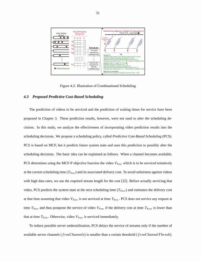
51

v2

Vn P

redic

ted

Stream

V3

Pre

dic

ted

Stream

V2

Pre

dic

ted

Stream

V1

Pre

dic

ted

Stream

S4

Sm

T3

Determining objective function for sequence SjFind all Possible

Sequences

X1 X2 X3 XnCurrent

Scheduling

Time

T2T1 Tn

Virtual Time

v1

v3

v4

vL

v5

Video Waiting

Queues

For each

sequence Sj

estimate F(Sj)

Waiting Request

Scheduler

S1

S2

S3

At time T1:Initialize total request count (N) and total cost (C) to zero;Add the number of waiting requests for V1 to N;Determine the required stream length and add it to C;Estimate next service time : T2 = next stream completion time;

At time Ti for i > 1 and Ti < T1 + Wp:Estimate number of arrivals in [Ti-1,Ti];Add the estimated number of arrivals to N;Determine the required stream length and add it to C;Estimate next service time : Ti+1 = next stream completion time;

Wp

After Wp is exceeded:Determine the sequence objective function F(Sj) = C/N;

Service the

sequence Sj

with the

smallest F(Sj)

Figure 4.2: Illustration of Combinational Scheduling

4.3 Proposed Predictive Cost-Based Scheduling

The prediction of videos to be serviced and the prediction of waiting times for service have been

proposed in Chapter 3. These prediction results, however, were not used to alter the scheduling de-

cisions. In this study, we analyze the effectiveness of incorporating video prediction results into the

scheduling decisions. We propose a scheduling policy, calledPredictive Cost-Based Scheduling(PCS).

PCS is based on MCF, but it predicts future system state and uses this prediction to possibly alter the

scheduling decisions. The basic idea can be explained as follows. When achannel becomes available,

PCS determines using the MCF-P objective function the videoVNow which is to be serviced tentatively

at the current scheduling time (TNow) and its associated delivery cost. To avoid unfairness against videos

with high data rates, we use the required stream length for the cost [22]. Before actually servicing that

video, PCS predicts the system state at the next scheduling time (TNext) and estimates the delivery cost

at that time assuming that videoVNow is not serviced at timeTNow. PCS does not service any request at

time TNow and thus postpone the service of videoVNow if the delivery cost at timeTNext is lower than

that at timeTNow. Otherwise, videoVNow is serviced immediately.

To reduce possible server underutilization, PCS delays the service of streams only if the number of

available server channels (f reeChannels) is smaller than a certain threshold (f reeChannelT hresh).

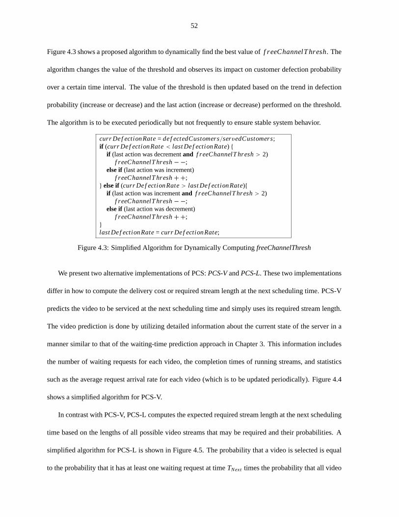
52

Figure 4.3 shows a proposed algorithm to dynamically find the best value off reeChannelT hresh. The

algorithm changes the value of the threshold and observes its impact on customer defection probability

over a certain time interval. The value of the threshold is then updated based on the trend in defection

probability (increase or decrease) and the last action (increase or decrease) performed on the threshold.

The algorithm is to be executed periodically but not frequently to ensure stable system behavior.

curr Def ectionRate= def ectedCustomers/servedCustomers;if (curr Def ectionRate< last Def ectionRate) {

if (last action was decrementand f reeChannelT hresh> 2)f reeChannelT hresh− −;

else if(last action was increment)f reeChannelT hresh+ +;

} else if(curr Def ectionRate> last Def ectionRate){if (last action was incrementand f reeChannelT hresh> 2)

f reeChannelT hresh− −;else if(last action was decrement)

f reeChannelT hresh+ +;}

last Def ectionRate= curr Def ectionRate;

Figure 4.3: Simplified Algorithm for Dynamically ComputingfreeChannelThresh

We present two alternative implementations of PCS:PCS-VandPCS-L. These two implementations

differ in how to compute the delivery cost or required stream length at the next scheduling time. PCS-V

predicts the video to be serviced at the next scheduling time and simply uses its required stream length.

The video prediction is done by utilizing detailed information about the currentstate of the server in a

manner similar to that of the waiting-time prediction approach in Chapter 3. This information includes

the number of waiting requests for each video, the completion times of running streams, and statistics

such as the average request arrival rate for each video (which is to be updated periodically). Figure 4.4

shows a simplified algorithm for PCS-V.

In contrast with PCS-V, PCS-L computes the expected required stream length at the next scheduling

time based on the lengths of all possible video streams that may be required andtheir probabilities. A

simplified algorithm for PCS-L is shown in Figure 4.5. The probability that a video is selected is equal

to the probability that it has at least one waiting request at timeTNext times the probability that all video

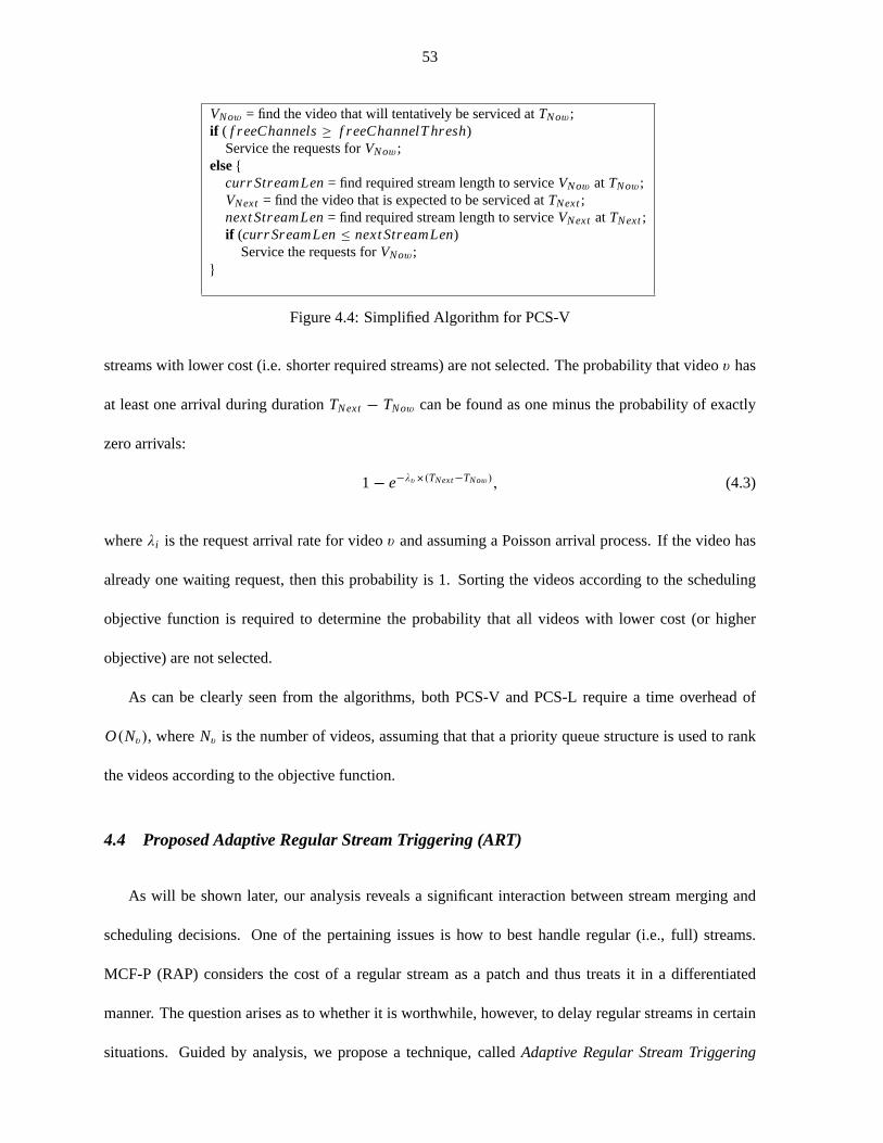
53

VNow = find the video that will tentatively be serviced atTNow;if ( f reeChannels≥ f reeChannelT hresh)

Service the requests forVNow;else{

curr StreamLen= find required stream length to serviceVNow at TNow;VNext = find the video that is expected to be serviced atTNext;next StreamLen= find required stream length to serviceVNext at TNext;if (curr SreamLen≤ next StreamLen)

Service the requests forVNow;}

Figure 4.4: Simplified Algorithm for PCS-V

streams with lower cost (i.e. shorter required streams) are not selected. The probability that videov has

at least one arrival during durationTNext − TNow can be found as one minus the probability of exactly

zero arrivals:

1 − e−λv×(TNext−TNow), (4.3)

whereλi is the request arrival rate for videov and assuming a Poisson arrival process. If the video has

already one waiting request, then this probability is 1. Sorting the videos according to the scheduling

objective function is required to determine the probability that all videos with lower cost (or higher

objective) are not selected.

As can be clearly seen from the algorithms, both PCS-V and PCS-L requirea time overhead of

O(Nv), whereNv is the number of videos, assuming that that a priority queue structure is usedto rank

the videos according to the objective function.

4.4 Proposed Adaptive Regular Stream Triggering (ART)

As will be shown later, our analysis reveals a significant interaction between stream merging and

scheduling decisions. One of the pertaining issues is how to best handle regular (i.e., full) streams.

MCF-P (RAP) considers the cost of a regular stream as a patch and thustreats it in a differentiated

manner. The question arises as to whether it is worthwhile, however, to delay regular streams in certain

situations. Guided by analysis, we propose a technique, calledAdaptive Regular Stream Triggering

54

VNow = find the video that will tentatively be serviced atTNow;if ( f reeChannels≥ f reeChannelT hresh)


curr StreamLen= find required stream length to serviceVNow at TNow;Calculate objective function for each video atTNext;Sort videos from best to worst according to objective function;expectedStreamLen= 0; // initialization// loop to find expected stream length at TNext

for (v = 0; v < Nv ; v + +){ // for each videonext StreamLen= find required stream length to servicev at TNext;Prob(videov is selected) = Prob(no other video with better objective is selected)

* Prob(videov has at least one arrival);expectedStreamLen+=Prob(videov is selected ) *next StreamLen;

}

if (curr SreamLen≤ expectedStreamLen)Service the requests forVNow;

}

Figure 4.5: Simplified Algorithm for PCS-L

(ART). A possible implementation is shown in Figure 4.6. The basic idea here is todelay regular

streams as long as the number of free channels is below a certain threshold,which is to be computed

dynamically based on the current workload and system state. ART uses thesame algorithm (shown in

Figure 4.3) to dynamically find the best value off reeChannelT hreshas that of PCS.

VNow = find the video that will be serviced atTNow;if ( f reeChannels≥ f reeChannelT hresh)


curr StreamLen= find the required stream length to serveVNow at TNow;if (curr StreamLen< mov ieLen) // not a full stream

Service the requests forVNow;else//full stream

Postpone the requests forVNow;}

Figure 4.6: Simplified Implementation of ART

To further demonstrate the main idea of ART, Figure 4.7 plots the ERMT merge tree without and

with ART, respectively. The solid lines show the initial stream lengths and the dotted lines show later

extensions. The circles identify successive extensions. With ART, thereis a gap before a regular stream

55

is initiated because of the postponement. We also observe that ART enhances the stream merging deci-

sions of ERMT. The number of initial regular streams (calledI Streamsin this study) in the merge tree is

relatively much smaller with ART. For example, there is only oneI Streamin the merge tree with ART

while there are many moreI Streamsin the merge tree without ART.

7.25 7.3 7.35 7.4

x 106

0

20

40

60

80

100

120

Vid

eo P

layb

ack

Poi

nt (m

inut

es)

Time

(a) MCF-P without ART

7.25 7.3 7.35 7.4

x 106

0

20

40

60

80

100

120

Vid

eo P

layb

ack

Poi

nt (m

inut

es)

Time

(b) MCF-P with ART

Figure 4.7: Impact of ART on ERMT Stream Merge Tree [Video 11, MCF-P, Server Capacity = 450]

As can be seen form the ART algorithm in Figure 4.6, ART requires a time overhead ofO(1) in

addition to the time overhead of the base scheduling policy used.

In principle, ART can be used with any scheduling policy, including PCS, although some negative

interference happens when it is combined with PCS, as will be shown in Section 4.6.

4.5 Evaluation Methodology

We study the effectiveness of the proposed policies through simulation. The simulation, written in

C, stops after a steady state analysis with 95% confidence interval is reached.

56

4.5.1 Workload Characteristics

Table 4.1 summarizes the workload characteristics used. Like most prior studies, we generally

Table 4.1: Summary of Workload CharacteristicsParameter Model/Value(s)Request Arrival Poisson Process (default)

Weibull Distribution with shapek = 0.6 to 0.9Request Arrival Rate Variable, Default is 40 Req./minServer Capacity 200 to 750 channelsVideo Access Zipf-LikeVideo Skew (θ ) 0.1 to 0.6, Default = 0.271Number of Videos Variable, Default is 120Video Length Fixed-Length Video Workload (Default)

with length of 60 to 180 min (same for all videos),Default = 120 min

Variable-Length Video Workload:with lengths randomly in the range: 60 to 180 min

Waiting Tolerance Model A, B, C, Default is AWaiting Tolerance Mean (µtol ) Variable, Default is 30 secFlash Crowds The peak arrival rate is 40 times the normal rate for a period of

two movie lengths and flash crowds arrival rate is variable.Default: no flash crowds

assume that the arrival of the requests to the server follows a Poisson Process with an average arrival

rateλ. We also experiment with the Weibull distribution with two parameters: shape andscale [68].

We analyze the impact of the shape (k), while adjusting the scale so that the desired average request

arrival rate is reached. Additionally, we assume that the access to videosis highly localized and follows

a Zipf-like distribution. With this distribution, the probability of choosing the nth most popular video

is C/n1−θ with a parameterθ and a normalized constant C. The parameterθ controls the skew of

video access. Note that the skew reaches its peak whenθ = 0, and that the access becomes uniformly

distributed whenθ = 1. We analyze the impact of this parameter, but we generally assume a value of

0.271 [66, 65].

We characterize the waiting tolerance of customers by three models. InModel A, the waiting tol-

erance follows an exponential distribution with meanµtol [66, 65]. In Model B, users with expected

waiting times less thanµtol will wait and the others will have the same waiting tolerance as Model A

[66, 65]. We useModel C from Chapter 3 to capture situations in which users either wait or defect

57

immediately depending on the expected waiting times. The user waits if the expectedwaiting time is

less thanµtol and defects immediately if the waiting time is greater than 2µtol . Otherwise, the defection

probability increases linearly from 0 to 1 for the expected waiting times betweenµtol and 2µtol .

As in most previous studies, we generally study a server with 120 videos, each of which is 120

minutes long. We examine the server at different loads by fixing the request arrival rate at 40 requests

per minute and varying the number of channels (server capacity) generally from 200 to 750. In addition

to the fixed-length video workload (in which all videos have the same length),we experiment with a

variable-length video workload. Moreover, we study the impacts of arrival rate, user’s waiting tolerance,

number of videos, and video length (in the fixed-length workload).

Flash crowds workload characteristics were adopted from [69].

4.5.2 Considered Performance Metrics

To evaluate the effectiveness of the proposed schemes, we consider the main performance metrics

discussed in Section 2.1. In addition, we analyze waiting-time predictability by twometrics: waiting-

time prediction accuracy and the percentage of clients receiving expectedwaiting times. The waiting-

time prediction accuracy is determined by the average deviation between the expected and actual waiting

times. For waiting-time prediction, we use the algorithm in Chapter 3. Note that this algorithm may not

provide an expected waiting time to each client because the prediction may not always be performed

accurately.


4.6.1 Comparing the Effectiveness of Different Cost-Computation Alternatives

Let us start by studying the effectiveness of Lookahead and Combinational Scheduling. Interestingly,

there is no clear benefit for computing the cost over a future period of time.In some cases, as shown in

Figure 4.8, the performance in term of customer defection and average waiting time may be worse than

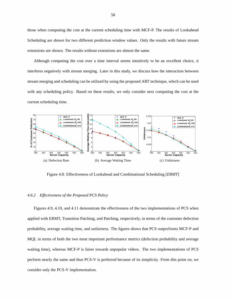
58

those when computing the cost at the current scheduling time with MCF-P. Theresults of Lookahead

Scheduling are shown for two different prediction window values. Only the results with future stream

extensions are shown. The results without extensions are almost the same.

Although computing the cost over a time interval seems intuitively to be an excellent choice, it

interferes negatively with stream merging. Later in this study, we discuss how the interaction between

stream merging and scheduling can be utilized by using the proposed ART technique, which can be used

with any scheduling policy. Based on these results, we only consider nextcomputing the cost at the

current scheduling time.

300 350 400 450 500 550 6000

10

20

30

40

50

60

70

80

% o

f Cus

tom

er D

efec

tion

Server Capacity

MCF−P Lookahead, W

p=50

Lookahead, Wp=150

Combinational, n=4

(a) Defection Rate

300 350 400 450 500 550 6000

2

4

6

8

10

12

14

16

Ave

rage

Wai

ting

Tim

e (s

econ

ds)

Server Capacity


p=50

Lookahead, Wp=150

Combinational, n=4

(b) Average Waiting Time

300 350 400 450 500 550 6000

0.005

0.01

0.015

0.02

0.025

Unf

airn

ess

Server Capacity


p=50

Lookahead, Wp=150

Combinational, n=4

(c) Unfairness

Figure 4.8: Effectiveness of Lookahead and Combinational Scheduling[ERMT]

4.6.2 Effectiveness of the Proposed PCS Policy

Figures 4.9, 4.10, and 4.11 demonstrate the effectiveness of the two implementations of PCS when

applied with ERMT, Transition Patching, and Patching, respectively, in termsof the customer defection

probability, average waiting time, and unfairness. The figures shows thatPCS outperforms MCF-P and

MQL in terms of both the two most important performance metrics (defection probability and average

waiting time), whereas MCF-P is fairer towards unpopular videos. The two implementations of PCS

perform nearly the same and thus PCS-V is preferred because of its simplicity. From this point on, we

consider only the PCS-V implementation.

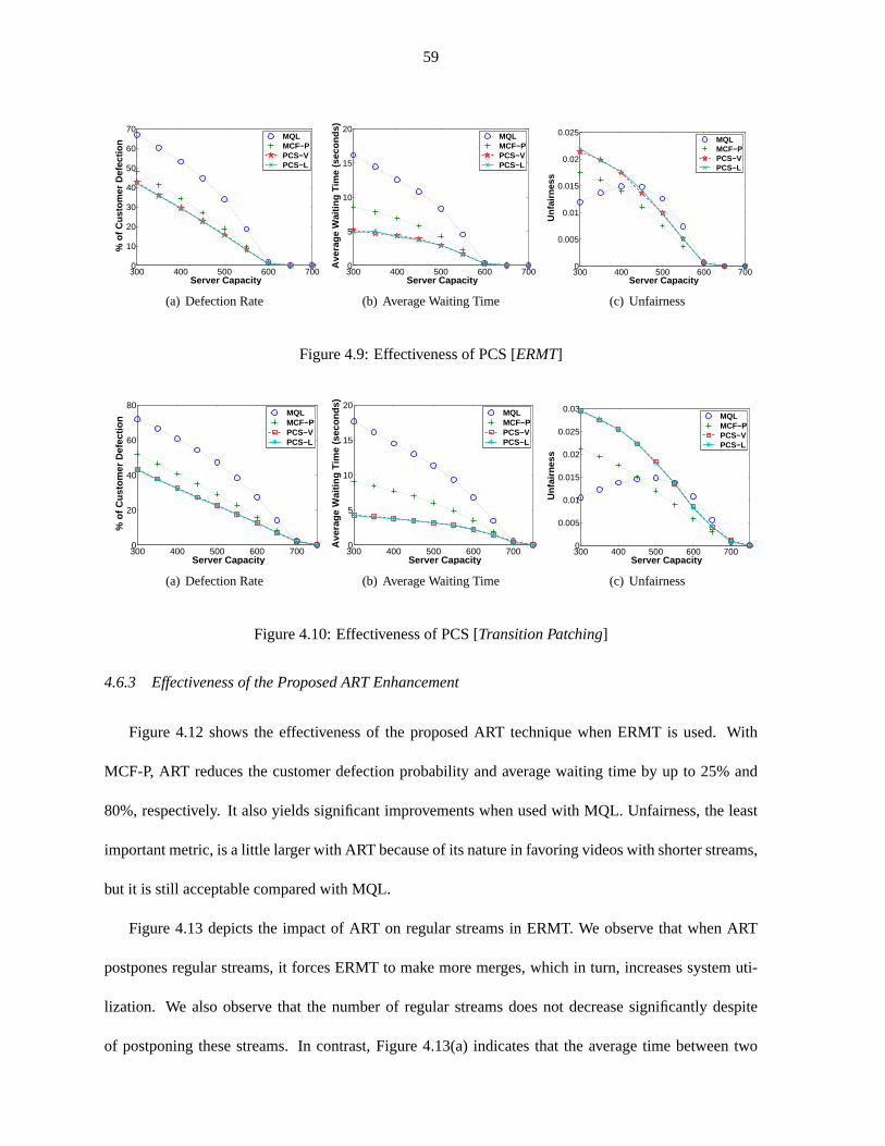
59

300 400 500 600 7000

10

20

30

40

50

60

70 %

of C

usto

mer

Def

ectio

n

Server Capacity

MQL MCF−P PCS−V PCS−L

(a) Defection Rate

300 400 500 600 7000

5

10

15

20

Ave

rage

Wai

ting

Tim

e (s

econ

ds)

Server Capacity



300 400 500 600 7000

0.005

0.01

0.015

0.02

0.025

Unf

airn

ess

Server Capacity


(c) Unfairness

Figure 4.9: Effectiveness of PCS [ERMT]

300 400 500 600 7000

20

40

60

80

% o

f Cus

tom

er D

efec

tion

Server Capacity


(a) Defection Rate

300 400 500 600 7000

5

10

15

20

Ave

rage

Wai

ting

Tim

e (s

econ

ds)

Server Capacity



300 400 500 600 7000

0.005

0.01

0.015

0.02

0.025

0.03

Unf

airn

ess

Server Capacity


(c) Unfairness

Figure 4.10: Effectiveness of PCS [Transition Patching]

4.6.3 Effectiveness of the Proposed ART Enhancement

Figure 4.12 shows the effectiveness of the proposed ART technique when ERMT is used. With

MCF-P, ART reduces the customer defection probability and average waitingtime by up to 25% and

80%, respectively. It also yields significant improvements when used with MQL. Unfairness, the least

important metric, is a little larger with ART because of its nature in favoring videoswith shorter streams,

but it is still acceptable compared with MQL.

Figure 4.13 depicts the impact of ART on regular streams in ERMT. We observe that when ART

postpones regular streams, it forces ERMT to make more merges, which in turn, increases system uti-

lization. We also observe that the number of regular streams does not decrease significantly despite

of postponing these streams. In contrast, Figure 4.13(a) indicates that theaverage time between two

60

300 400 500 600 70010

20

30

40

50

60

70

80 %

of C

usto

mer

Def

ectio

n

Server Capacity


(a) Defection Rate

300 400 500 600 7000

5

10

15

20

Ave

rage

Wai

ting

Tim

e (s

econ

ds)

Server Capacity



300 400 500 600 7000.005

0.01

0.015

0.02

0.025

0.03

Unf

airn

ess

Server Capacity


(c) Unfairness

Figure 4.11: Effectiveness of PCS [Patching]

successive regular streams for popular videos is even smaller with ART than that without it. This is

because ERMT keeps extending streams, which eventually become regularstreams. Figures 4.13(b) and

4.13(c) compare the percentage of initial regular streams (I Streams) and extended regular streams (E

Streams) without and with ART, respectively. We can see that the percentage of extended regular streams

with ART is much higher. This supports the fact that the number of regular streams is not reduced by

postponing. In summary, we can say that ART improves ERMT by replacing many I Streamswith E

Streams.

300 350 400 450 500 550 6000

10

20

30

40

50

60

70

% o

f Cus

tom

er D

efec

tion

Server Capacity

MQL MCF−P MQL with ART MCF−P with ART

(a) Defection Rate

300 350 400 450 500 550 6000

5

10

15

20

Ave

rage

Wai

ting

Tim

e (s

econ

ds)

Server Capacity



300 400 500 6000

0.005

0.01

0.015

0.02

0.025

0.03

Unf

airn

ess

Server Capacity


(c) Unfairness

Figure 4.12: Effectiveness of ART [ERMT]

Let us now discuss the impact of ART when Transition Patching and Patchingare used. Transition

Patching results are presented in Figure 4.14 and Patching results are presented in Figure 4.15. As

with ERMT, ART reduces significantly the customer defection probability and the average waiting time

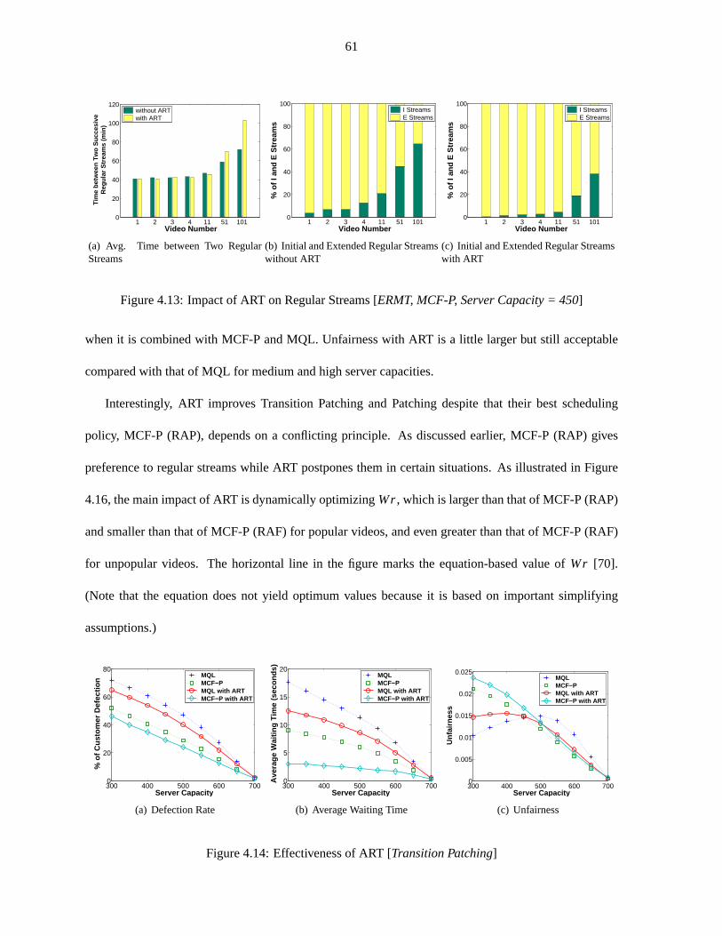
61

1 2 3 4 11 51 1010

20

40

60

80

100

120 T

ime

betw

een

Tw

o S

ucce

sive

Reg

ular

Str

eam

s (m

in)

Video Number

without ART with ART

(a) Avg. Time between Two RegularStreams

1 2 3 4 11 51 1010

20

40

60

80

100

% o

f I a

nd E

Str

eam

s

Video Number

I Streams E Streams

(b) Initial and Extended Regular Streamswithout ART

1 2 3 4 11 51 1010

20

40

60

80

100

% o

f I a

nd E

Str

eam

s

Video Number

I Streams E Streams

(c) Initial and Extended Regular Streamswith ART

Figure 4.13: Impact of ART on Regular Streams [ERMT, MCF-P, Server Capacity = 450]

when it is combined with MCF-P and MQL. Unfairness with ART is a little larger butstill acceptable

compared with that of MQL for medium and high server capacities.

Interestingly, ART improves Transition Patching and Patching despite that their best scheduling

policy, MCF-P (RAP), depends on a conflicting principle. As discussed earlier, MCF-P (RAP) gives

preference to regular streams while ART postpones them in certain situations. As illustrated in Figure

4.16, the main impact of ART is dynamically optimizingWr, which is larger than that of MCF-P (RAP)

and smaller than that of MCF-P (RAF) for popular videos, and even greater than that of MCF-P (RAF)

for unpopular videos. The horizontal line in the figure marks the equation-based value ofWr [70].

(Note that the equation does not yield optimum values because it is based on important simplifying

assumptions.)

300 400 500 600 7000

20

40

60

80

% o

f Cus

tom

er D

efec

tion

Server Capacity


(a) Defection Rate

300 400 500 600 7000

5

10

15

20

Ave

rage

Wai

ting

Tim

e (s

econ

ds)

Server Capacity



300 400 500 600 7000

0.005

0.01

0.015

0.02

0.025

Unf

airn

ess

Server Capacity


(c) Unfairness

Figure 4.14: Effectiveness of ART [Transition Patching]

62

300 400 500 600 70010

20

30

40

50

60

70

80 %

of C

usto

mer

Def

ectio

n

Server Capacity


(a) Defection Rate

300 400 500 600 7000

5

10

15

20

Ave

rage

Wai

ting

Tim

e (s

econ

ds)

Server Capacity



300 400 500 600 7000.005

0.01

0.015

0.02

0.025

Unf

airn

ess

Server Capacity


(c) Unfairness

Figure 4.15: Effectiveness of ART [Patching]

550 600 650 700 750 800 8500

2

4

6

8

10

12

Act

ual W

r (m

inut

es)

Server Capacity

MCF−P(RAF) MCF−P(RAP) MCF−P(RAP) with ART

(a) Video 1

550 600 650 700 750 800 8500

5

10

15

20

25

30

35

Act

ual W

r (m

inut

es)

Server Capacity


(b) Video 10

550 600 650 700 750 800 8500

10

20

30

40

Act

ual W

r (m

inut

es)

Server Capacity


(c) Video 20

Figure 4.16: Comparing ActualWr in MCF-P (RAF), MCF-P (RAP), and MCFP(RAP) with ART[Patching]

4.6.4 Comparing the Effectiveness of PCS and ART

Although ART can be applied with any scheduling policy, including PCS, for the time being, we

consider it as an alternative to PCS because of negative interference between the two, as will be shown

in Subsection 4.6.8. In this subsection, we compare the effectiveness of PCS-V and ART in terms of

customer defection probability, average waiting time, unfairness against unpopular videos, and cost per

request. Figures 4.17, 4.18, and 4.19 shows the results of ERMT, Transition Patching, and Patching

respectively.

With ERMT, MCF-P when combined with ART performs better than PCS-V in terms of the customer

defection probability and average waiting time. The results when Transition Patching and Patching are

used exhibit different behavior than those with ERMT. MCF-P combined withART gives almost the

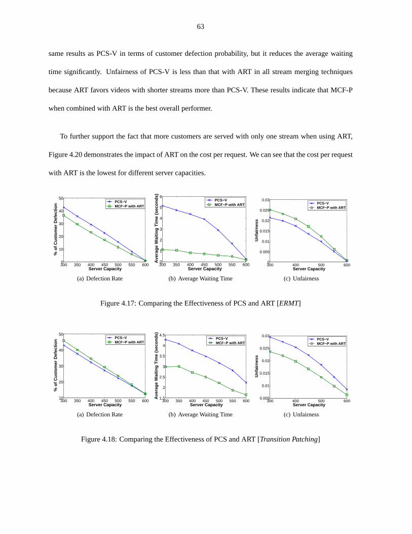
63

same results as PCS-V in terms of customer defection probability, but it reduces the average waiting

time significantly. Unfairness of PCS-V is less than that with ART in all stream merging techniques

because ART favors videos with shorter streams more than PCS-V. Theseresults indicate that MCF-P

when combined with ART is the best overall performer.

To further support the fact that more customers are served with only onestream when using ART,

Figure 4.20 demonstrates the impact of ART on the cost per request. We cansee that the cost per request

with ART is the lowest for different server capacities.

300 350 400 450 500 550 6000

10

20

30

40

50

% o

f Cus

tom

er D

efec

tion

Server Capacity

PCS−V MCF−P with ART

(a) Defection Rate

300 350 400 450 500 550 6000

1

2

3

4

5

6

Ave

rage

Wai

ting

Tim

e (s

econ

ds)

Server Capacity



300 400 500 6000

0.005

0.01

0.015

0.02

0.025

0.03

Unf

airn

ess

Server Capacity


(c) Unfairness

Figure 4.17: Comparing the Effectiveness of PCS and ART [ERMT]

300 350 400 450 500 550 60010

20

30

40

50

% o

f Cus

tom

er D

efec

tion

Server Capacity


(a) Defection Rate

300 350 400 450 500 550 6001.5

2

2.5

3

3.5

4

4.5

Ave

rage

Wai

ting

Tim

e (s

econ

ds)

Server Capacity



300 400 500 6000.005

0.01

0.015

0.02

0.025

0.03

Unf

airn

ess

Server Capacity


(c) Unfairness

Figure 4.18: Comparing the Effectiveness of PCS and ART [Transition Patching]

64

300 350 400 450 500 550 60025

30

35

40

45

50

55

60

% o

f Cus

tom

er D

efec

tion

Server Capacity


(a) Defection Rate

300 350 400 450 500 550 6003

4

5

6

7

Ave

rage

Wai

ting

Tim

e (s

econ

ds)

Server Capacity



300 400 500 6000.015

0.02

0.025

0.03

Unf

airn

ess

Server Capacity


(c) Unfairness

Figure 4.19: Comparing the Effectiveness of PCS and ART [Patching]

20 40 60 80 100 1200

500

1000

1500

2000

2500

Ave

rage

Cos

t Per

Req

uest

(sec

onds

)

Video Number


(a) 300 channel

20 40 60 80 100 1200

500

1000

1500

2000

2500

Ave

rage

Cos

t Per

Req

uest

(sec

onds

)

Video Number


(b) 400 channel

20 40 60 80 100 1200

500

1000

1500

2000

2500

Ave

rage

Cos

t Per

Req

uest

(sec

onds

) Video Number


(c) 500 channel

Figure 4.20: Comparing the Impacts of PCS and ART on Cost per Request [ERMT, MCF-P]

4.6.5 Impact of Workload Parameters on the Effectiveness of PCS and ART

Figures 4.21, 4.22, 4.23, and 4.24 illustrate the impact of the request arrival rate, customer waiting

tolerance, number of videos and video length on the effectiveness of PCS-V and ART. The results

for both Patching and ERMT are shown. The results demonstrate that ART always achieves smaller

customer defection probability and average waiting time than PCS-V in the case of ERMT. In Patching,

the same trend is observed for the average waiting time, but PCS-V and “MCF-P combined with ART”

perform nearly the same in terms of customer defection probability, especiallywhen the server is highly

loaded.

Figure 4.25 shows that the skew in video access has significant impacts on the customer defection

probability, average waiting time and unfairness. Recall that asθ increases, the skew in video access

65

20 40 60 80 100 1200

10

20

30

40

50

60

70 %

of C

usto

mer

Def

ectio

n

Request Rate (Requests/Minute)

Patching, PCS−V ERMT, PCS−V Patching, MCF−P with ART ERMT, MCF−P with ART

(a) Defection Rate

20 40 60 80 100 1200

2

4

6

8

10

Ave

rage

Wai

ting

Tim

e (s

econ

ds)




20 40 60 80 100 1200

0.01

0.02

0.03

0.04

0.05

Unf

airn

ess



(c) Unfairness

Figure 4.21: Impact of Request Arrival Rate [Server Capacity = 500]

20 30 40 50 60 700

10

20

30

40

50

60

% o

f Cus

tom

er D

efec

tion

Average Waiting Tolerance (seconds)


(a) Defection Rate

20 30 40 50 60 700

5

10

15

Ave

rage

Wai

ting

Tim

e (s

econ

ds)




20 30 40 50 60 700

0.005

0.01

0.015

0.02

0.025

0.03

0.035

0.04

Unf

airn

ess



(c) Unfairness

Figure 4.22: Impact of Customer Waiting Tolerance [Server Capacity = 500]

decreases. Both the defection probability and average waiting time are worsen by the reduction in the

skew. This is because cost-based scheduling policies favor popular videos by nature. Whenθ increases,

the deference in video popularity decreases which in turn make the scheduling decision harder to make.

Unfairness decreases by increasingθ which is as expected. Again, “MCF-P combined with ART” is the

best policy in term of all performance metrics, except unfairness.

The results so far are for a video workload of a fixed video length. Figure 4.26 shows the customer

defection probability, average waiting time and unfairness results for a variable-length video workload.

The workload is comprised of videos with lengths in the range of 60 to 180 minutes. The length of each

video is generated randomly within the specified range. The results for the workload are obtained by

averaging the values of four runs. The PCS-V and ART algorithms also work well in this workload.

66

100 150 2000

10

20

30

40

50

60 %

of C

usto

mer

Def

ectio

n

Number of Videos


(a) Defection Rate

100 150 2000

2

4

6

8

10

Ave

rage

Wai

ting

Tim

e (s

econ

ds)

Number of Videos



100 150 2000

0.005

0.01

0.015

0.02

0.025

0.03

0.035

Unf

airn

ess

Number of Videos


(c) Unfairness

Figure 4.23: Impact of Number of Videos [Server Capacity = 500]

60 80 100 120 140 160 1800

10

20

30

40

50

60

% o

f Cus

tom

er D

efec

tion

Video Length (Minutes)


(a) Defection Rate

60 80 100 120 140 160 1800

1

2

3

4

5

6

7

8

9

Ave

rage

Wai

ting

Tim

e (s

econ

ds)




60 80 100 120 140 160 1800

0.005

0.01

0.015

0.02

0.025

0.03

0.035

0.04

Unf

airn

ess



(c) Unfairness

Figure 4.24: Impact of Video Length [Server Capacity = 500]

“MCF-P combined with ART” as in most cases performs better than all other policies. Moreover, we

can see that the fairness of ART and PCS-V is better than that of MCF-P withvariable-length video

workload.

The results so far assume a Poisson request arrival process. Let us now examine the behavior under

Weibull distribution with different shape (k) values. Figure 4.27 demonstrates that the shape has a little

impact, especially when the server capacity is larger than 500 channels. Figure 4.28 compares MCF-P,

PCS-V, and MCF-P with ART under Weibull Arrival Distribution with the same shape. The results with

other shape parameters have the same trend and thus are not shown. We can see clearly that PCS-V and

“MCF-P combined with ART” sill perform better than MCF-P. We can see alsothat MCF-P with ART

is the best policy.

67

0.1 0.2 0.3 0.4 0.5 0.60.1

0.15

0.2

0.25

0.3

0.35

% o

f Cus

tom

er D

efec

tion



(a) Defection Rate

0.1 0.2 0.3 0.4 0.5 0.60

2

4

6

8

10

Ave

rage

Wai

ting

Tim

e (s

econ

ds)




0.1 0.2 0.3 0.4 0.5 0.60.005

0.01

0.015

0.02

0.025

Unf

airn

ess



(c) Unfairness

Figure 4.25: Impact of Skew in Video Access [ERMT, Server Capacity = 450]

200 250 300 350 400 450 5000

0.5

1

1.5

2

2.5

% o

f Cus

tom

er D

efec

tion

Server Capacity

MCF−P PCS−V MCF−P with ART

(a) Defection Rate

200 250 300 350 400 450 5000

5

10

15

20

25

30

35

40

Ave

rage

Wai

ting

Tim

e (s

econ

ds)

Server Capacity



200 250 300 350 400 450 5000

0.02

0.04

0.06

0.08

0.1

Unf

airn

ess

Server Capacity


(c) Unfairness

Figure 4.26: Comparing the Effectiveness of MCF-P, PCS, and ART under a Variable-Length VideoWorkload [ERMT, 60 to 180 minutes Video Length Range]

4.6.6 Comparing Waiting-Time Predictability with PCS and ART

Figure 4.29 compares the predictability of MCF-P, PCS-V, and “MCF-P combined with ART” in

terms of the average deviation and percentage of clients receiving expected time of service (PCRE)

under waiting tolerance Model B. The results with Model C are similar and thusare not shown. The

results demonstrate that ART significantly improves the predictability of MCF-P.PCS-V is also more

predictable than MCF-P. In particular, ART reduces the average deviation by up to 30% and 75% for

models B and C, respectively. It also increases the number of clients receiving expected times by up to

35%. Moreover, “MCF-P combined with ART” gives more customers expected times than PCS-V with

a relatively less significant increase in the average deviation.

68

300 350 400 450 500 550 6000

0.1

0.2

0.3

0.4

0.5

% o

f Cus

tom

er D

efec

tion

Server Capacity

K = 0.60 K = 0.70 K = 0.82 K = 0.86 K = 0.90

(a) Defection Rate

300 350 400 450 500 550 6000

1

2

3

4

5

6

7

Ave

rage

Wai

ting

Tim

e (s

econ

ds)

Server Capacity

K = 0.60 K = 0.70 K = 0.82 K = 0.86 K = 0.90


300 350 400 450 500 550 6000

0.005

0.01

0.015

0.02

0.025

Unf

airn

ess

Server Capacity

K = 0.60 K = 0.70 K = 0.82 K = 0.86 K = 0.90

(c) Unfairness

Figure 4.27: Impact of the Shape Parameter of Weibull Arrival Distribution[ERMT, PCS-V]

300 350 400 450 500 550 6000

0.1

0.2

0.3

0.4

0.5

0.6

0.7

% o

f Cus

tom

er D

efec

tion

Server Capacity


(a) Defection Rate

300 350 400 450 500 550 6000

2

4

6

8

10

12

Ave

rage

Wai

ting

Tim

e (s

econ

ds)

Server Capacity



300 350 400 450 500 550 6000

0.005

0.01

0.015

0.02

0.025

0.03

Unf

airn

ess

Server Capacity


(c) Unfairness

Figure 4.28: Comparing MCF-P, PCS-V, and MCF-P with ART under WeibullArrival Distribution[ERMT, K = 0.6]

4.6.7 Impact of Flash Crowds on the Effectiveness of PCS and ART

Let us now discuss the impact of flash crowds on the effectiveness of PCS-V and ART. Figure 4.30

demonstrates the impact of flash crowds inter-arrival time on MCF-P, PCS-V, and “MCF-P combined

with ART”. The results show that MCF-P when combined with ART handles the flash crowds more

efficiently than the other policies. In particular, it achieves the best customer defection probability and

average waiting time under all flash crowds inter-arrival times. PCS-V achieves better results than MCF-

P, but it is improvement is less than that of ART. Figure 4.31 confirms that ARTenhances the efficiency

of stream handling even with flash crowds. It is clearly evident that “MCF-P combined with ART”

achieves the lowest cost per request for all videos.

69

300 400 500 600 7000

0.5

1

1.5

2

Ave

rage

Dev

iatio

n (s

econ

ds)

Server Capacity



300 400 500 600 700

0.4

0.5

0.6

0.7

0.8

0.9

1

% o

f Use

rs W

ith E

xpec

ted

Tim

es

Server Capacity


(b) Customer With Expected Time

Figure 4.29: Waiting-Time Predictability of MCF-P, MCF-P with ART, and PCS-V[ERMT, Wp =

0.5µtol , Model B]

0.5 1 2 3 4 5 6 7 42

44

46

48

50

52

54

56

% o

f Cus

tom

er D

efec

tion

Flash Crowds Interarrival Time (days)


(a) Customer Defection

0.5 1 2 3 4 5 6 7 0

2

4

6

8

10

Ave

rage

Wai

ting

time

(sec

onds

)



(b) Waiting Time

0.5 1 2 3 4 5 6 7 0.02

0.022

0.024

0.026

0.028

0.03

0.032

Unf

airn

ess



(c) Unfairness

Figure 4.30: Impact of Flash Crowds on MCF-P, PCS-V, and ART as a Function of Flash Crowds Iner-arrival Time [ERMT, Server capacity = 300]

4.6.8 Effectiveness of Combining ART with PCS

Let us now look at the results of combining PCS-V with ART. We show the results under ERMT and

Patching in Figures 4.32 and 4.33, respectively. Transition Patching has the same trend as Patching and

therefore its results are not shown. These results indicate that “MCF-P combined with ART” performs

the best among all variations, and that PCS-V performs better than “PCS-Vwith ART”. From these

figures, we conclude that negative interference occurs when ART is combined with PCS-V. Removing

this interference by modifying these two strategies is a challenging task and left for a future study.

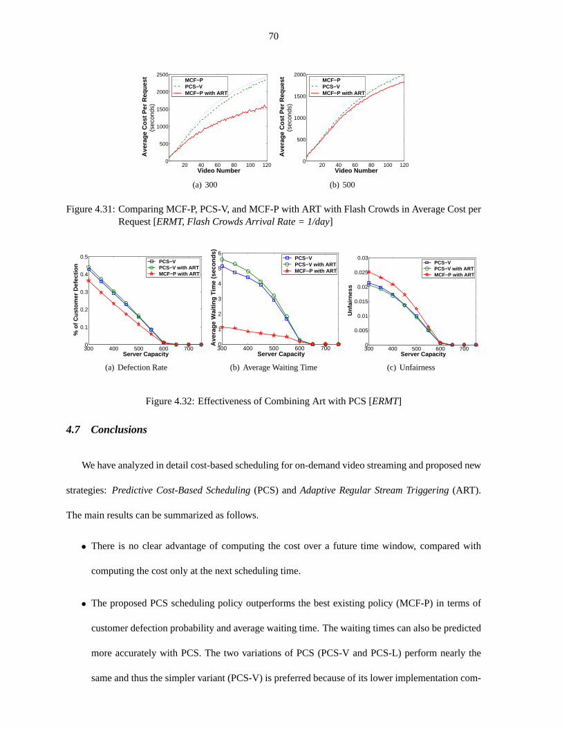
70

20 40 60 80 100 1200

500

1000

1500

2000

2500

Ave

rage

Cos

t Per

Req

uest

(sec

onds

)

Video Number


(a) 300

20 40 60 80 100 1200

500

1000

1500

2000

Ave

rage

Cos

t Per

Req

uest

(sec

onds

)

Video Number


(b) 500

Figure 4.31: Comparing MCF-P, PCS-V, and MCF-P with ART with Flash Crowds in Average Cost perRequest [ERMT, Flash Crowds Arrival Rate = 1/day]

300 400 500 600 7000

0.1

0.2

0.3

0.4

0.5

% o

f Cus

tom

er D

efec

tion

Server Capacity

PCS−V PCS−V with ART MCF−P with ART

(a) Defection Rate

300 400 500 600 7000

1

2

3

4

5

6

Ave

rage

Wai

ting

Tim

e (s

econ

ds)

Server Capacity



300 400 500 600 7000

0.005

0.01

0.015

0.02

0.025

0.03

Unf

airn

ess

Server Capacity


(c) Unfairness

Figure 4.32: Effectiveness of Combining Art with PCS [ERMT]

4.7 Conclusions

We have analyzed in detail cost-based scheduling for on-demand video streaming and proposed new

strategies:Predictive Cost-Based Scheduling(PCS) andAdaptive Regular Stream Triggering(ART).


• There is no clear advantage of computing the cost over a future time window,compared with

computing the cost only at the next scheduling time.

• The proposed PCS scheduling policy outperforms the best existing policy (MCF-P) in terms of

customer defection probability and average waiting time. The waiting times can alsobe predicted

more accurately with PCS. The two variations of PCS (PCS-V and PCS-L) perform nearly the

same and thus the simpler variant (PCS-V) is preferred because of its lower implementation com-

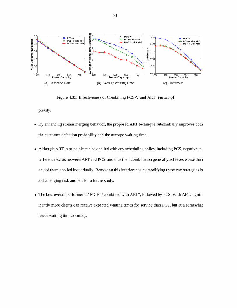
71

300 400 500 600 7000.1

0.2

0.3

0.4

0.5

0.6

% o

f Cus

tom

er D

efec

tion

Server Capacity


(a) Defection Rate

300 400 500 600 7001

2

3

4

5

6

7

Ave

rage

Wai

ting

Tim

e (s

econ

ds)

Server Capacity



300 400 500 600 7000.005

0.01

0.015

0.02

0.025

0.03

Unf

airn

ess

Server Capacity


(c) Unfairness

Figure 4.33: Effectiveness of Combining PCS-V and ART [Patching]

plexity.

• By enhancing stream merging behavior, the proposed ART technique substantially improves both

the customer defection probability and the average waiting time.

• Although ART in principle can be applied with any scheduling policy, including PCS, negative in-

terference exists between ART and PCS, and thus their combination generally achieves worse than

any of them applied individually. Removing this interference by modifying thesetwo strategies is

a challenging task and left for a future study.

• The best overall performer is “MCF-P combined with ART”, followed by PCS. With ART, signif-

icantly more clients can receive expected waiting times for service than PCS, but at a somewhat

lower waiting time accuracy.

72

CHAPTER 5

DISTORTION-BASED CROSS-LAYER OPTIMIZATION FORWIRELESS VIDEO STREAMING

5.1 Introduction

In this study, we consider video streaming from multiple video sources (or stations) to a central

station over a single-hop IEEE 802.11 wireless LAN (WLAN) network. Thisapplication is typical

in Automated Video Surveillance (AVS) systems. As shown in Figure 1.2, the wireless video sources

(video cameras or sensors) share the same medium and can be either battery-powered or outlet-powered.

The central proxy station is connected with a high-bandwidth link to the access point, and thus this link

is not deemed as a bottleneck in the system. Large systems may be composed of multiple such systems

or cells.

The main challenge in the considered system is that the wireless network has limited available band-

width, which should be estimated accurately and distributed efficiently among various video sources.

Our ultimate goal in this study is to build a cross-layer framework for maximizing thenetwork band-

width utilization. This cross-layer approach, clarified in Figure 5.1, utilizes and may adapt parameters

from the application, link, and physical layers of the network layer stack.The problem is to be for-

mulated using the AVS intuitive rate-accuracy function. The objective of theoptimization will be to

maximize the sum of the weighted accuracy of vision algorithms running in the system, where the

weights are the importance factors of the video sources in the system.

Distortion-based bandwidth optimization in such systems has been addressedin only few studies [43,

44] by using cross-layer optimization and as discussed in Section 2.5, thesesolutions are highly limited.

For this reason and for comparative purposes, we propose a distortion-based cross-layer framework

that dynamically manages the available network bandwidth in such a way that minimizes the overall

distortion. The proposed cross-layer framework utilizes an online approach for estimating the effective

73

Video SourceVideo SourceVideo SourceVideo Source

Application

Layer

Application Layer

Characteristics

MAC

Physical Layer

Mac

Characteristics

Physical

Characteristics

Optimal Video

Streaming Rate

Optimal Parameter

Set

Cross Layer

Optimization

Algorithm At the

Access Point

A message from

the AP

A message to

the AP

Wireless Video Sources

eq

eq

Figure 5.1: Cross Layer Framework Clarification

airtime of the network. To yield an accurate estimation, the proposed approach computes the effective

airtime when the packet loss is below a specified threshold.

We evaluate the proposed solution by streaming real video frames (and notjust an abstract bit stream)

over a simulated network. The simulations are conducted using OPNET. Sincethe sent video packets

may be lost, we implement an error concealment algorithm [71] at the proxy station to mitigate the

impact of packet loss on perceptual video quality. We also study the performance of the proposed

framework with the existence of other interfering/cross traffic in the network.

The main contributions of this part of the dissertation can be summarized as follows. (1) We propose

a complete cross-layer optimization framework, including a new online and dynamic approach for esti-

mating the effective airtime of the network. (2) We develop a new and accurate model that characterizes

the relationship between the video data rate and the distortion. (3) We propose an enhanced online and

dynamic approach for estimating the effective airtime of the network. (4) We develop a new model for

adapting the link layer parameters in the video sources. (5) We test our framework by streaming real

video frames over a simulated network and incorporating an error concealment algorithm to mitigate the

impact of video packet loss. (6) We study the impact of interfering/cross traffic on the performance of

the proposes framework.

The results show that the proposed framework enhances substantially theperceptual quality of re-

74

ceived video streams and that the proposed effective airtime estimation algorithm is accurate and con-

verges quickly. The proposed framework also results in much less powerconsumption, compared with

existing solutions. This behavior is due to sending and dropping much less data. Power consumption is

a primary concern, especially when the video sources are battery-powered. Moreover, results shows that

the proposed framework is highly adaptable for any interfering traffic in the network.

The rest of this chapter is organized as follows. Table 5.1 summarizes the notations that are used

in this study and their definitions. Section 5.2 presents the proposed cross-layer optimization frame-

work. Subsequently, Section 5.3 discusses the performance evaluation methodology. Finally, Section

5.4 presents and analyzes the main results.

Table 5.1: Notations SummaryNotation DefinitionCWmin Minimum Contention WindowCWmax Maximum Contention WindowAP Access PointAC Access CategoryAIFS Arbitration Inter Frame SpaceTXOP Transmission Opportunity TimeS Number of video sourcesrs Rate of the encoded video sent by source sys Source s physical rateAef f the effective airtime of the mediumfs Airtime fraction of source sτ Frame rateZ Video frame sizets Throughput of source s video stream as received by the application layer of the proxy stationds source s data dropping rateA1 The overall average dropping ratio,A1 =

∑Ss=1 ds/ys.

Athresh A threshold that controls the allowable dropping in the networkλ Lagrangian constantas, bs, cs Distortion curve constantsxs Optimized TXOP limitRs Maximum load rate measured by the MAC layer at source sLs Maximum video frame size at source sNs Number of MAC layer data frames per maximum video frame at source sls Average data load per MAC layer data frame at source sOs Average MAC and physical layers overhead at source sts Short Interframe Space (SIFS) timeta Time required to send an acknowledgment

75

5.2 Proposed Cross-Layer Optimization Framework

This study considers a system of video streaming from multiple video sources(or stations) to a

central station over a single-hop IEEE 802.11 WLAN network in EDCA mode.As shown in Figure 1.2,

the system hasS ≥ 1 video sources and each sources streams a different encoded video at rateRs. Each

video sources may have a different physical rate (ys).

The ultimate goal of this study is to provide an optimal solution that dynamically distributes and

allocates the available network bandwidth among various video sources. This solution should consider

all system, video, network, and environmental aspects, which may changedynamically. Therefore, the

proposed cross-layer optimization solution utilizes and dynamically controls parameters in three layers

in the network stack: Application, Link, and Physical.

5.2.1 Cross-Layer Optimization Problem Formulation

As in [44], we formulate the problem as a cross-layer optimization problem ofthe sum of the dis-

tortion of all video streams received by the central proxy station. We followthe formulation in [44], but

adapt it to include the packetization overhead of the transport and application layers. Since all video

sources share the same medium, the bandwidth allocation solution should determine the fraction of

airtime that each video source receives in the system. Obviously, the total airtime cannot exceed the

effective airtime of the medium. Specifically, the problem is formulated as: find the optimal fraction of

the airtime allocationF∗ = { f ∗s |s = 1, 2, 3, ..., S} for various video sources that minimizes the total

distortion (∑S

s=1 Distortions(rs)), wherers is the application layer transfer rate for video sources, and

S is the number of video sources. This optimization is subject to the following constraints. (1) The total

airtime of all video sources is less than the effective airtime of the medium (Aef f ). (2) The application

layer transfer rate of sources is the product of the its airtime (fs) and the physical layer transfer rate (ys)

for video sources. (3) The airtime of each source is between 0 and 1 (inclusive).

76

Mathematically, the problem can be stated as follows:

Find F∗ = arg minF

S∑

s=1

Distortion(rs) (5.1a)

s.t.S

∑

s=1

fs = Aef f (5.1b)

rs = fs × ys (5.1c)

0 ≤ fs ≤ 1 (5.1d)

s = 1, 2, 3, ..., S, (5.1e)

whereF∗ is the set of optimal fractions (f ∗s ) of the airtime of all sources,r ∗

s is the optimal application-

layer rate of video sources, ys is the physical-layer rate of video sources, andAef f is the total effective

airtime.

To solve the problem formulated in Equation (5.1), we need to characterize the distortion function

and assess the effective airtime of the network.

5.2.2 Distortion Function Characterization

We seek to find a model of the relationship between the size of a JPEG snapshot (or alternatively the

rate of an MJPEG video) and the distortion of the snapshot. We determine the size-distortion relationship

based on the following image data sets: CMU/MIT [72], Georgia Tech [73],FERET [74], and SCFace

[75]. We also use these image sets in our experiments to assemble the MJPEG video streams using

the streamer discussed in Section 5.3 to load the network with video traffic. Forfair evaluations of

bandwidth allocation solutions, each video source should be able to stream the video at a bitrate that

matches that of the optimization solution. The Georgia Tech image set producesa highly limited range

of bitrates for the studied network. To produce a better variety, we generate another image set from

the original Georgia Tech image set by changing the resolution of each image inthe set to 50% of the

77

original resolution. The new image set have a resolution of 320× 240. For each image set, we use the

IJG JPEG library to compress each picture in the set with quality factors from1 to 100, with 1 being

the lowest, and then assess the distortion of each image against the original image using the Root Mean

Square Error (RMSE) metric. Finally, we find the average size and the average distortion of all images

with the same quality factor. The results are shown in Figure 5.2. These results indicate that the model

formulated in [76] (identified as “Existing Model”) is not accurate. We determine that the distortion can

be better characterized as follows:

Distortion(RMSE) = a × Zb + c, (5.2)

whereZ is the image size anda, b, c are constants. This model is referred to as “New Model” in Figure

6.1. For MJPEG videos, image sizeZ can be calculated asZ = R/τ , whereR is the video playback

rate andτ is the video frame rate.

5.2.3 Effective Airtime Estimation

As finding an accurate value for the effective airtime of the medium is necessary for solving the

formulated optimization problem, we propose a novel online and dynamic effective airtime estima-

tion algorithm for wireless networks in infrastructure configuration. In contrast with existing analytical

models, the algorithm uses complete information about the network and involvesthe cooperation of the

access point and all video sources as well as various layers in each source. The algorithm does not incur

additional network traffic and can be executed only when significant changes in the network (such as

variations in the physical rates) happen.

As shown in Figure 5.3, the algorithm proceeds as follows. First, for eachvideo sources, it finds

the throughput (ts) of its video stream as received by the application layer of the proxy station, when

all sources stream videos, each at a rate that is equal to the maximum physical rate of the network

78

0.02 0.04 0.06 0.08 0.1 0.120

5

10

15

20

Dis

tort

ion

(RM

SE

)

Size (MB)

Real Data Existing Model New Model

(a) CMU/MIT

0.01 0.02 0.03 0.040

5

10

15

20

Dis

tort

ion

(RM

SE

)

Size (MB)


(b) Georgia Tech

0.01 0.02 0.03 0.04 0.050

5

10

15

Dis

tort

ion

(RM

SE

)

Size (MB)


(c) FERET

2 4 6 8 10 12

x 10−3

0

5

10

15

20

Dis

tort

ion

(RM

SE

)

Size (MB)


(d) SCFace

Figure 5.2: Size-Distortion Models

divided by the number of sources [77]. The algorithm then uses this throughput to determine the initial

value of the effective airtime (Aef f ) as follows: Aef f =∑S

s=1 ts/ys. Our experiments indicate that this

initial value significantly overestimates the effective airtime, causing the actualreceived video rates to

not conform to the cross-layer optimization solution because of the high level of packet packet dropping

in the network. Thus, this value has to be adjusted based on the experienced level of packet dropping.

Subsequently, during a period of time, called estimation period, each video sources assesses its own

data dropping rate (ds) while sending its video stream, and then sends this information to the access point

(AP). Meanwhile, the AP determines the overall average dropping ratio asfollows: A1 =∑S

s=1 ds/ys.

A1 is used to adjust the current value ofAef f at the end of the current estimation period. IfA1 is

greater than some thresholdAthresh, the AP reducesAef f by A1 − Athresh. Athreshcontrols the allowable

dropping in the network. IfA1, however, is less thanAthresh, the AP increasesAef f by a valueI , which

79

set as half the last increment or decrement value, depending on whetherthe last operation is increment or

decrement, respectively. Guided by extensive experiments, we setI to half the last decrement/increment

to ensure better convergence and stability. The algorithm terminates when theincrements become less

than a thresholdI thresh. The estimation period andI thresh should be chosen based on the best tradeoff

between convergence and stability.

if this is the first time to run the algorithmAef f =

∑Ss=1 ts/ys;

At the end of each estimation period{

A1 =∑S

s=1 ds/ys;if (A1 < Athresh){

if (last operation was decrement){

I = 0.5 ∗ last Decrement;Aef f = Aef f + I ;}

else if(last operation was increment){

I = 0.5 ∗ I ;Aef f = Aef f + I ;}

else//no decrements happened before//keep increasingAef f to cause the first decrementAef f = Aef f+ 0.05 ;

if (last Increment< I thresh)Stop the estimation algorithm;

}

else if(A1 ≥ Athresh){Aef f = Aef f − (A1 − Athresh);last Decrement= A1 − Athresh;}

}

Figure 5.3: The Algorithm for Dynamically Estimating the Effective Airtime

5.2.4 Enhanced Effective Airtime Estimation

By studying the online estimation algorithm proposed in the previous section in details, we have

found some options for further enhancements. One of these enhancements is to eliminate the initial

period that the algorithm spend to find an initial value forAef f to start with. We find that starting with

a moderate initial value such as 0.5 is sufficient. The other enhancement thatcan be done is to make

the incrementing step of the algorithm directly dependent on the desiredAthresh. By doing this, the

algorithm become more stable and converges to a more accurate effective airtime value. By employing

80

these enhancements, the resulting algorithm came out to be much simpler, easierto calibrate, and uses

less design parameters. Figure 5.4 shows the enhanced algorithm.

The algorithm starts with initializingAef f with 0.5. This statement is only executed once when the

system start running. Next, as in the algorithm in the previous section, during a period of time called

estimation period, each video sources assesses its own data dropping rate (ds) while sending its video

stream, and then sends this information to the access point (AP). Meanwhile,the AP determines the

overall average dropping ratio as follows:A1 =∑S

s=1 ds/ys. A1 is then used to adjust the current value

of Aef f at the end of the current estimation period. IfA1 came out to be zero,Aef f is incremented by

Athresh. If A1 is greater than the thresholdAthresh, the AP reducesAef f by C∗(A1− Athresh) where C is

a positive constant. IfA1, however, is less thanAthresh, the AP increasesAef f by C∗(Athresh− A1). The

estimation period and the constantC should be chosen based on the best tradeoff between convergence

and stability.

Initialize Aef f with 0.5At the end of each estimation period{

A1 =∑S

s=1 ds/ys;if (A1 == 0)

Aef f = Aef f + Athresh;else if(A1 < Athresh)

Aef f = Aef f + C ∗ (Athresh− A1);else if(A1 > Athresh)

Aef f = Aef f − C ∗ (A1 − Athresh);}

Figure 5.4: Enhanced Effective Airtime Estimation Algorithm

5.2.5 Cross-Layer Optimization Solution

Now that we have a distortion function and a value for the effective airtime, we can solve the prob-

lem formulated in Equation (5.1). The problem solution can be summarized as follows:

Step 1: We first prove that the formulated problem is a convex programming problemby determining

that all constraints ((6.1b)-(6.1e)) in the problem are linear and thus convex and that the optimization

81

function (∑S

s=1(as( fsys/τs)bs + cs)) is also convex. The latter is valid since the derivative of the sum

term is monotonically non-decreasing and convex.

Step 2:Since the problem is a budget constrained convex programming problem, it can be solved using

the Lagrangian relaxation technique [78]. Thus, we can write the followingLagrangian-relaxed formula:

L(F∗, λ) =

S∑

s=1

(as( fsys/τs)bs + cs) + λ(

S∑

s=1

fs − Aef f ), (5.3)

where 0≤ fs ≤ 1, ands = 1, 2, 3, ..., S. Next, the Lagrangian conditions are formulated as follows:

∂L

∂ fs= 0 and

∂L

∂λ= 0. (5.4)

Assuming that all video sources have the samebs, which is empirically valid, solving these two equations

yields the following solution:

f ∗s = (

−λ∗τs

asbsys(ys/τs)(bs−1))(1/(bs−1)), (5.5)

where

λ∗ = (Aef f

∑Ss=1(

−τsasbsys(ys/τs)(bs−1) )

(1/(bs−1)))(bs−1). (5.6)

5.2.6 Enforcing the Optimization Results

With the aforementioned solution, the AP determinesλ∗ and then each video sources determines

its fraction of the airtimef ∗s after receivingλ∗ from the AP. Subsequently, each video sources should

change the application data rate, which is the video encoding rate in this case,as follows: r ∗s = f ∗

s ×

ys. Finally, the link-layer parameters are determined based on the allocated airtimefor each source.

The link-layer parameters can either be the transmission opportunity durationlimit (TXOP limit) or

alternatively the frequency of the transmission opportunity. The control of the TXOP limit is more

82

preferred since it is only one parameter, whereas the transmission frequency involves three parameters

(AIFS, CWmin, andCWmax), which complicates the control process design.

In [44], the TXOP limit (x∗s ) for sources is determined as the time required to transmit the number of

MAC data frames that sources can transmit during one beacon interval time (tb). As discussed in Section

5.4.3, our results show that choosing intervals other the beacon interval can achieve better performance.

In particular, the received video quality improves with the chosen time intervalup to a certain point,

and then it starts to worsen. In addition, the time interval that achieves the best results varies with the

network size. Furthermore, the model in [44] does not incorporate the packetization overhead of the

transport and application layers.

In our framework, we address these problems as follows. Each video source determines its TXOP

limit as the time required to transmit the packets that belong to a single video frame along with all

associated overhead. Because of the cross-layer approach, the MAC layer in sources can know the

frame rateτs of the video sent by the application layer in that source. The MAC layer canalso determine

the maximum load rateRs coming from the source’s upper layers. Using this information, we can

determine the maximum video frame sizeLs (with overhead) asRs/τs and the number of MAC layer

data frames per maximum video frameNs as Ls/ ls, wherels is the average data load per MAC layer

data frame. Given thatOs is the average MAC and physical layers overhead,ts is Short Interframe

Space (SIFS)time, andta is the time required to send an acknowledgment, TXOP limit can be found as

follows:

x∗s = [

Ls

ys] + [

OsNs

ys] + [(2Ns − 1)ts] + [Nsta], (5.7)

where Lsys

is the time required for transmitting the data of a single video frame and the overhead of the

upper layers associated with that video frame,OsNsys

is the time required for transmitting the associated

MAC and physical layers overhead,(2Ns− 1)ts is the sum of theSIFSperiods needed for transmitting

all the packets of the video frame, andNsta is the time required for receiving all the acknowledgment

83

packets of the video frame packets.

5.3 Performance Evaluation Methodology

We use the OPNET simulator to conduct various experiments. In contrast withprior studies, which

deal with video streams as abstract data streams with certain bitrates, we implement a traffic source

in OPNET that streams MJPEG videos as Real-time Transport Protocol (RTP) packets. Moreover, we

implement a realistic video streaming client at the application layer of the proxy station. This client

receives and reassembles the RTP packets from various video streams,and then carries out error con-

cealment to mitigate the impact of packet loss. The use of MJPEG enables the use of standard image

data sets that are suitable for surveillance applications because the MJPEGvideo stream is a set of JPEG

images. We use the the following image sets to assemble the video streams: CMU/MIT[72], Georgia

Tech [73], and FERET [74]. The streamer at each source takes a bitrate, a frame rate, and an image set

as inputs and produces a corresponding MJPEG video stream.

As shown in Figure 5.1, the implementation of the proposed framework is distributed between the

video sources and the AP. Each video source send its state information (physical rate, data dropping rate,

and Rate-Distortion curve characteristics) to the AP periodically using a newmanagement packet. This

packet can be calledstate report[44]. The AP can than calculateλ∗ using Equation 5.6 and distribute it

using the beacon packet. Each video sources than usesλ∗ from the received beacon packet to calculate

f ∗s according to Equation 5.5 that is used eventually by sources to calculate its optimal application rate

according to Equation 5.1c and its optimal TXOP limit time using Equation 5.7.

For comparative purposes, we implement the cross-layer algorithm proposed in [44], referred to

here asDistortion Optimization (DO). Our proposed solution is referred to asEnhanced Distortion

Optimization (EDO). We also compare the results with standard EDCA. In addition, we implement a

variation of the standard EDCA, calledAdaptive EDCA, in which the application layer in each video

source adapts its video rate according to the physical rate of that source, and thus the rate is set asys/S.

84

We analyze the followingperformance metrics.

• Perceptual Video Quality- It is the main metric and is measured in the overall Peak Signal to Noise

Ratio (PSNR). We set the PSNR of missed frames to 0.

• Average video packet delay- The average time needed for the access point to receive a video data

packet sent by a video source. The average video packet delay is anessential metric due to the

real-time playback requirement.

• Average percentage of received complete video frames.

• Average percentage of received incomplete video frames.

• Average percentage of missed video frames.

• Overall network load- It is defined as the total load sent from the application layers of all sources.

• Overall dropping rate due to buffer overflow.

• Overall dropping rate due to reaching the retransmission limit.

• Power Consumption- It is the average power consumption of the wireless interfaces of the video

sources and is determined by using the power consumption model proposedin [79] for MJPEG

video streaming.

Since the proposed cross-layer framework utilizes a dynamic and online effective airtime estimator

that estimates the useful fraction of the airtime that can be used for surveillance traffic, the framework

adapts the sending rates of the video sources to achieve the best performance with the existence of any

other interfering/cross data traffic in the network. To show the impact of thisinterfering/cross traffic on

the performance of the proposed framework, we conduct various experiments with 8 none-video sources

that are sharing the same wireless medium of the surveillance system. These none-video sources send

best effort traffic to the access point all with the same pr-specified rate.We perform experiments with

three packet rates of cross traffic. Cross traffic 1 sources send packets with 0.005 seconds inter-arrival

time. In cross traffic 2 sources, we set the inter-arrival time to 0.003 second while we set the inter-arrival

85

time to 0.001 seconds in cross traffic 3 sources.

Table 5.2 summarizes the main simulation parameters.

Table 5.2: Summary of Simulation ParametersParameter Model/Value(s)Number of video sources 10-44Simulation Time 10 minPacket Size 1024 bytesApplication Rate Optimized, Default = Max Physical Rate / No. of SourcesVideo Frame Rate 20 frames/secPhysical characteristics Extended Rate (802.11g)Physical Data Rate Random from{12Mb/s, 18Mb/s, 24Mb/s, 36Mb/s, 48Mb/s, 54Mb/s}

Weight One of five levels between [0 1] chosen randomlyBuffer size 256 KbVideo TXOP limit Optimized, Default = 3008µsVideoCWmin 15VideoCWmax 31Video AIFS 2Short Retry Limit 7Long Retry Limit 4Beacon Interval 0.02 secondState Report Interval 1 second

5.4 Results Presentation and Analysis

5.4.1 Effectiveness of Using the Cross-Layer Approach in Bandwidth Allocation

Let us start by demonstrating the benefits of utilizing information from different network layers in

bandwidth allocation. Figure 5.5 compares standard EDCA and adaptive EDCA in terms of PSNR.These

results indicate that adapting the application rate according to the physical rate in each video source (as

done in Adaptive EDCA) improves the PSNR by at least 50%!

5.4.2 Analysis of the Enhanced Effective Airtime Estimation Algorithm

Extensive analysis of the design parameters of the enhanced effectiveairtime estimation algorithm

indicates that their values are best set as follows to enhance the performance in terms of stability and

convergence:Athresh = 0.0075,C = 0.2, andEstimation Period= 5 seconds. Figure 5.6 shows the

effective airtime over the whole time of running the EDO solution using FERET image sets. Results

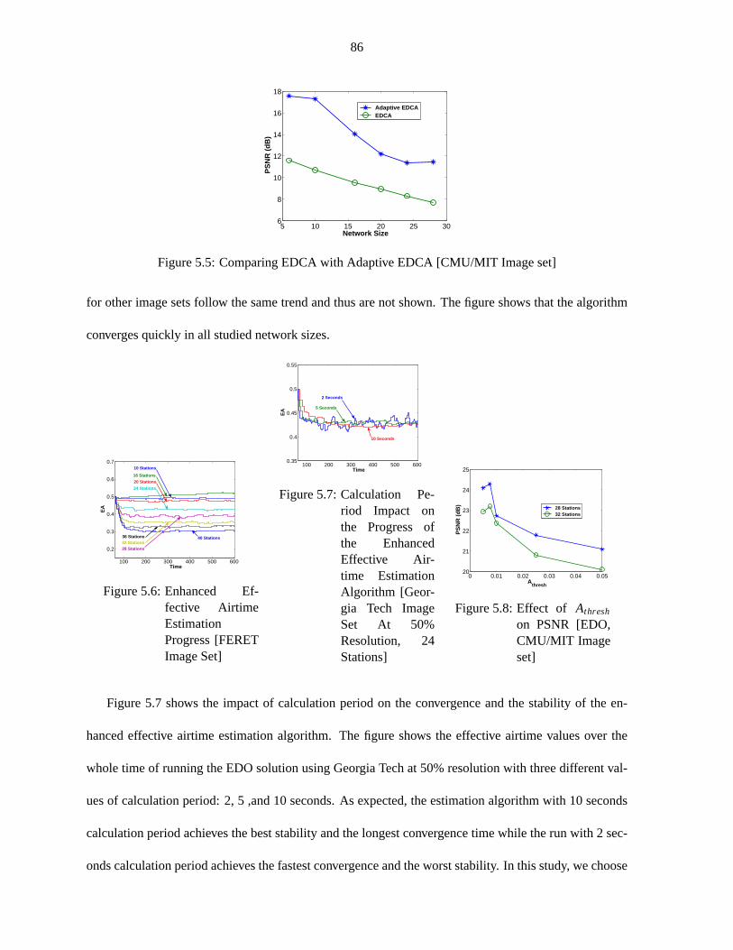
86

5 10 15 20 25 306

8

10

12

14

16

18

PS

NR

(dB

)

Network Size

Adaptive EDCA EDCA

Figure 5.5: Comparing EDCA with Adaptive EDCA [CMU/MIT Image set]

for other image sets follow the same trend and thus are not shown. The figure shows that the algorithm

converges quickly in all studied network sizes.

100 200 300 400 500 600

0.2

0.3

0.4

0.5

0.6

0.7

EA

Time

16 Stations

10 Stations

24 Stations

20 Stations

32 Stations36 Stations

28 Stations

40 Stations

Figure 5.6: Enhanced Ef-fective AirtimeEstimationProgress [FERETImage Set]

100 200 300 400 500 6000.35

0.4

0.45

0.5

0.55

EA

Time

10 Seconds

2 Seconds

5 Seconds

Figure 5.7: Calculation Pe-riod Impact onthe Progress ofthe EnhancedEffective Air-time EstimationAlgorithm [Geor-gia Tech ImageSet At 50%Resolution, 24Stations]

0 0.01 0.02 0.03 0.04 0.0520

21

22

23

24

25

PS

NR

(dB

)

Athresh

28 Stations 32 Stations

Figure 5.8: Effect of Athresh

on PSNR [EDO,CMU/MIT Imageset]

Figure 5.7 shows the impact of calculation period on the convergence and the stability of the en-

hanced effective airtime estimation algorithm. The figure shows the effectiveairtime values over the

whole time of running the EDO solution using Georgia Tech at 50% resolution withthree different val-

ues of calculation period: 2, 5 ,and 10 seconds. As expected, the estimationalgorithm with 10 seconds

calculation period achieves the best stability and the longest convergencetime while the run with 2 sec-

onds calculation period achieves the fastest convergence and the worst stability. In this study, we choose

87

5 seconds as our calculation period because it achieves very good trade-off between the convergence and

the stability of the estimation algorithm.

Impact of Athresh, which determines the allowable dropping in the network, on perceptual video

quality is shown in Figure 5.8. This figure depicts the results of running the proposed EDO solution for

two different network sizes: 28 and 32 stations. The results show that thequality of the received video

streams improves withAthreshup to a point and then the quality starts to worsen. The peak happens when

Athresh is smaller than 0.01, suggesting that that optimal perceptual video quality is achieved when the

dropping is very small.

5.4.3 Analysis of Link-Layer Adaptation

As discussed in Subsection 6.2.5, study [44] determines the TXOP limit (x∗s ) for sources as the

time required to transmit the number of MAC data frames that sources can transmit during one beacon

interval time (tb). Let us know discuss the impact of choosing time intervals other than the beacon

interval. Table 5.3 shows the PSNR when running the solution proposed in [44] (DO) for different

time intervals and network sizes. These results indicate that perceptual video quality improves with

increasing the chosen time interval until a peak is reached, and then it startsto worsen. Furthermore, the

best value of the time interval varies with the network size.

Table 5.3: Impact of the Time Interval Selected to Determine TXOP Limit on Perceptual Video Quality[PSNR (dB)]

TimeInterval

Network Size10 16 20 24

0.02 19.15 12.30 10.25 8.810.5 24.46 18.77 16.17 15.691 24.46 19.00 16.40 15.662 24.46 19.00 16.46 15.663 24.46 19.00 16.46 15.65

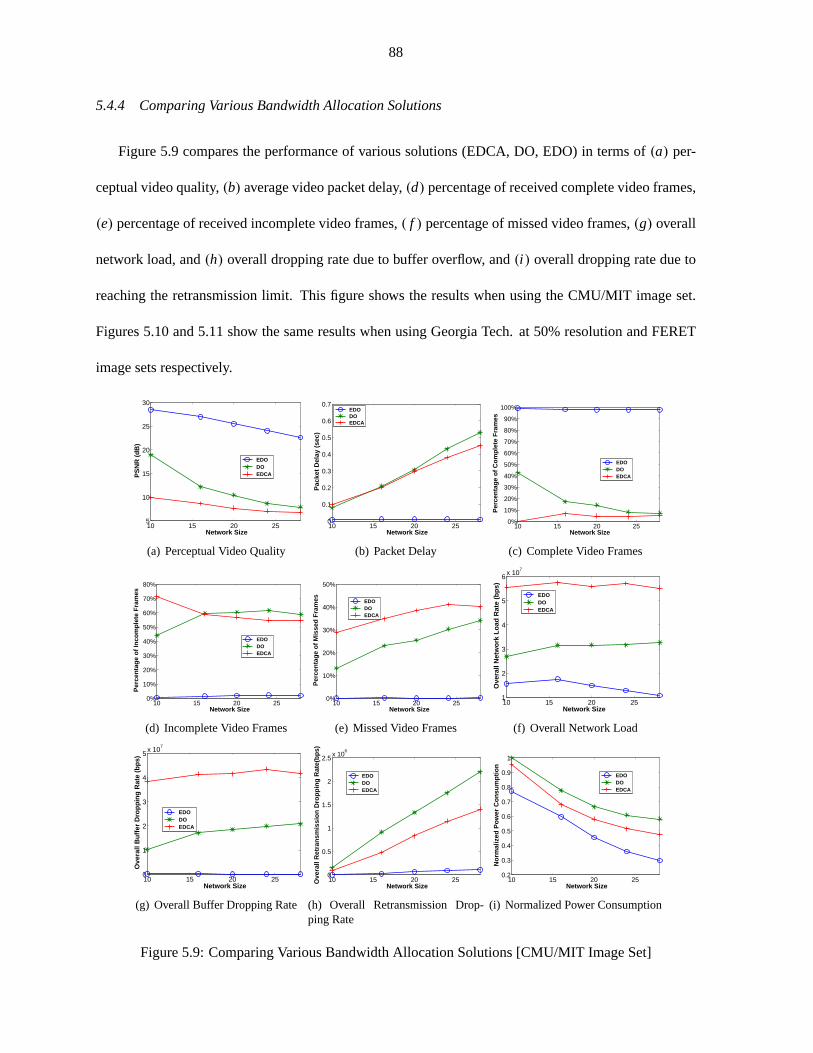
88

5.4.4 Comparing Various Bandwidth Allocation Solutions

Figure 5.9 compares the performance of various solutions (EDCA, DO, EDO) in terms of(a) per-

ceptual video quality,(b) average video packet delay,(d) percentage of received complete video frames,

(e) percentage of received incomplete video frames,( f ) percentage of missed video frames,(g) overall

network load, and(h) overall dropping rate due to buffer overflow, and(i ) overall dropping rate due to

reaching the retransmission limit. This figure shows the results when using the CMU/MIT image set.

Figures 5.10 and 5.11 show the same results when using Georgia Tech. at 50% resolution and FERET

image sets respectively.

10 15 20 255

10

15

20

25

30

PS

NR

(dB

)

Network Size

EDO DO EDCA

(a) Perceptual Video Quality

10 15 20 250

0.1

0.2

0.3

0.4

0.5

0.6

0.7

Pac

ket D

elay

(se

c)

Network Size

EDO DO EDCA

(b) Packet Delay

10 15 20 25 0%

10%

20%

30%

40%

50%

60%

70%

80%

90%

100%

Per

cent

age

of C

ompl

ete

Fra

mes

Network Size

EDO DO EDCA

(c) Complete Video Frames

10 15 20 25 0%

10%

20%

30%

40%

50%

60%

70%

80%

Per

cent

age

of In

com

plet

e F

ram

es

Network Size

EDO DO EDCA

(d) Incomplete Video Frames

10 15 20 25 0%

10%

20%

30%

40%

50%

Per

cent

age

of M

isse

d F

ram

es

Network Size

EDO DO EDCA

(e) Missed Video Frames

10 15 20 251

2

3

4

5

6x 10

7

Ove

rall

Net

wor

k Lo

ad R

ate

(bps

)

Network Size

EDO DO EDCA

(f) Overall Network Load

10 15 20 250

1

2

3

4

5x 10

7

Ove

rall

Buf

fer

Dro

ppin

g R

ate

(bps

)

Network Size

EDO DO EDCA

(g) Overall Buffer Dropping Rate

10 15 20 250

0.5

1

1.5

2

2.5x 10

6

Ove

rall

Ret

rans

mis

sion

Dro

ppin

g R

ate(

bps)

Network Size

EDO DO EDCA

(h) Overall Retransmission Drop-ping Rate

10 15 20 250.2

0.3

0.4

0.5

0.6

0.7

0.8

0.9

1

Nor

mal

ized

Pow

er C

onsu

mpt

ion

Network Size

EDO DO EDCA

(i) Normalized Power Consumption

Figure 5.9: Comparing Various Bandwidth Allocation Solutions [CMU/MIT ImageSet]

89

The results show that EDO significantly outperforms other studied solutions.In particular, it im-

proves PSNR by more than 100% compared with standard EDCA and by 20% to100% compared with

DO. In addition to that, we can see clearly that EDO almost eliminates video packet delay. Moreover,

EDO yields the highest percentage of completely received video frames and the lowest percentage of

incomplete and missed frames. This behavior is due to the effective airtime estimation algorithm, which

minimizes packet dropping and to the effective link-layer adaptation model used. Accordingly, EDO

reduces significantly the following three metrics: overall network load, buffer dropping rate , and re-

transmission dropping rate. These results indicate that EDO consumes much less processing power by

sending and dropping much less data. Finally, the results show that EDO significantly enhances the wire-

less interface power consumption at the video sources. It reduces the power consumption on average by

20%.

5.4.5 Impact of Interfering Traffic on the Performance of the ProposedBandwidth Allocation Solution

In this subsection, we analyze the impact of cross traffic with different data rates on the performance

of the studied bandwidth allocation solutions. Figures 5.12 and 5.13 show the results in terms of PSNR,

Packet Delay, and Normalized Power Consumption with Georgia Tech at 50%resolution and FERET

image sets respectively when using EDO solution. We show only the results in terms of these three

metrics because they summarize all other performance metrics. The results show that the proposed

framework is highly adaptable to cross traffic in the network. In particular,the degradation of PSNR and

average packet delay is almost negligible even with the highest data rate cross traffic (cross traffic 3).

Power consumption is less with cross traffic because the proposed framework adapts the video sources

and make them send video streams with lower rates.

Figures 5.14 and 5.15 compare EDO, DO, and EDCA all with cross traffic 2 interms of PSNR,

Packet Delay, and Normalized Power Consumption when using Georgia Tech at 50% resolution and

FERET image sets respectively. Figures 5.16 and 5.17 show the same resultswith cross traffic 3. Re-

90

10 15 20 25 30 35 405

10

15

20

25

30

35

PS

NR

(dB

)

Network Size

EDO DO EDCA


10 15 20 25 30 35 400

0.1

0.2

0.3

0.4

0.5

0.6

0.7

0.8

Pac

ket D

elay

(se

c)

Network Size

EDO DO EDCA

(b) Packet Delay

10 15 20 25 30 35 40 0%

10%

20%

30%

40%

50%

60%

70%

80%

90%

100%

Per

cent

age

of C

ompl

ete

Fra

mes

Network Size

EDO DO EDCA


10 15 20 25 30 35 40 0%

10%

20%

30%

40%

50%

60%

70%

Per

cent

age

of In

com

plet

e F

ram

es

Network Size

EDO DO EDCA


10 15 20 25 30 35 40 0%

10%

20%

30%

40%

50%

60%

Per

cent

age

of M

isse

d F

ram

es

Network Size

EDO DO EDCA


10 15 20 25 30 35 401

2

3

4

5

6x 10

7

Ove

rall

Net

wor

k Lo

ad R

ate

(bps

)

Network Size

EDO DO EDCA


10 15 20 25 30 35 400

1

2

3

4

5x 10

7

Ove

rall

Buf

fer

Dro

ppin

g R

ate

(bps

)

Network Size

EDO DO EDCA


10 15 20 25 30 35 400

0.5

1

1.5

2

2.5

3

3.5x 10

6

Ove

rall

Ret

rans

mis

sion

Dro

ppin

g R

ate(

bps)

Network Size

EDO DO EDCA


10 15 20 25 30 35 400.2

0.3

0.4

0.5

0.6

0.7

0.8

0.9

1

Nor

mal

ized

Pow

er C

onsu

mpt

ion

Network Size

EDO DO EDCA


Figure 5.10: Comparing Various Bandwidth Allocation Solutions [Georgia Tech Image Set At 50% Res-olution]

sults show that even with cross traffic, EDO outperform DO and EDCA significantly in terms of all

performance metrics.

Figures 5.18 and 5.19 compare EDO with cross traffic 3, DO and EDCA without any cross traffic

in terms of PSNR, Packet Delay, and Normalized Power Consumption when Georgia Tech at 50%

resolution and FERET image sets are used respectively. Despite the fact that EDO was running with the

highest data rate cross traffic and other solutions are running without any cross traffic, results show that

EDO still outperforms DO and EDCA significantly in terms of all studied performance metrics.

91

10 15 20 25 30 35 405

10

15

20

25

30

35

40

PS

NR

(dB

)

Network Size

EDO DO EDCA


10 15 20 25 30 35 400

0.1

0.2

0.3

0.4

0.5

0.6

0.7

0.8

Pac

ket D

elay

(se

c)

Network Size

EDO DO EDCA

(b) Packet Delay

10 15 20 25 30 35 40 0%

10%

20%

30%

40%

50%

60%

70%

80%

90%

100%

Per

cent

age

of C

ompl

ete

Fra

mes

Network Size

EDO DO EDCA


10 15 20 25 30 35 40 0%

10%

20%

30%

40%

50%

60%

70%

Per

cent

age

of In

com

plet

e F

ram

es

Network Size

EDO DO EDCA


10 15 20 25 30 35 40 0%

10%

20%

30%

40%

50%

60%

Per

cent

age

of M

isse

d F

ram

es

Network Size

EDO DO EDCA


10 15 20 25 30 35 401

2

3

4

5

6x 10

7

Ove

rall

Net

wor

k Lo

ad R

ate

(bps

)

Network Size

EDO DO EDCA


10 15 20 25 30 35 400

1

2

3

4

5x 10

7

Ove

rall

Buf

fer

Dro

ppin

g R

ate

(bps

)

Network Size

EDO DO EDCA


10 15 20 25 30 35 400

0.5

1

1.5

2

2.5

3

3.5x 10

6

Ove

rall

Ret

rans

mis

sion

Dro

ppin

g R

ate(

bps)

Network Size

EDO DO EDCA


10 15 20 25 30 35 400.2

0.3

0.4

0.5

0.6

0.7

0.8

0.9

1

Nor

mal

ized

Pow

er C

onsu

mpt

ion

Network Size

EDO DO EDCA


Figure 5.11: Comparing Various Bandwidth Allocation Solutions [FERET ImageSet]

5.5 Conclusions

We have proposed a cross-layer video optimization framework that manages the network bandwidth

to minimize the total distortion in video streams. The proposed framework utilizes a new online network

effective airtime estimation algorithm. Moreover, we have developed a new and accurate model for

characterizing the video data rate and distortion relationship as well as a newmodel for adapting the link-

layer parameters. We have evaluated our framework by streaming real video frames over an OPNET-

simulated wireless network.

The main results can be summarized as follows. (1) The proposed framework enhances substan-

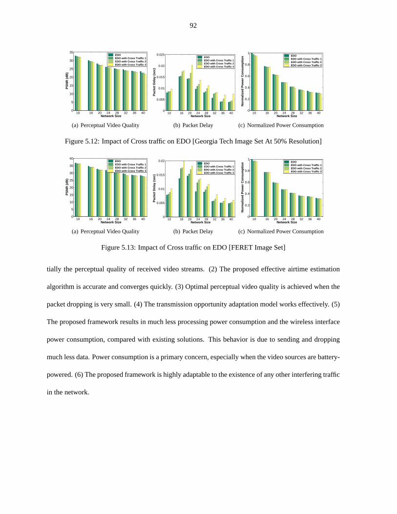
92

10 16 20 24 28 32 36 400

5

10

15

20

25

30

35

PS

NR

(dB

)

Network Size

EDO EDO with Cross Traffic 1 EDO with Cross Traffic 2 EDO with Cross Traffic 3


10 16 20 24 28 32 36 400

0.005

0.01

0.015

0.02

0.025

Pac

ket D

elay

(se

c)

Network Size


(b) Packet Delay

10 16 20 24 28 32 36 400

0.2

0.4

0.6

0.8

1

Nor

mal

ized

Pow

er C

onsu

mpt

ion

Network Size


(c) Normalized Power Consumption

Figure 5.12: Impact of Cross traffic on EDO [Georgia Tech Image Set At50% Resolution]

10 16 20 24 28 32 36 400

5

10

15

20

25

30

35

40

PS

NR

(dB

)

Network Size



10 16 20 24 28 32 36 400

0.005

0.01

0.015

0.02

Pac

ket D

elay

(se

c)

Network Size


(b) Packet Delay

10 16 20 24 28 32 36 400

0.2

0.4

0.6

0.8

1

Nor

mal

ized

Pow

er C

onsu

mpt

ion

Network Size



Figure 5.13: Impact of Cross traffic on EDO [FERET Image Set]

tially the perceptual quality of received video streams. (2) The proposedeffective airtime estimation

algorithm is accurate and converges quickly. (3) Optimal perceptual video quality is achieved when the

packet dropping is very small. (4) The transmission opportunity adaptation model works effectively. (5)

The proposed framework results in much less processing power consumption and the wireless interface

power consumption, compared with existing solutions. This behavior is due to sending and dropping

much less data. Power consumption is a primary concern, especially when thevideo sources are battery-

powered. (6) The proposed framework is highly adaptable to the existence of any other interfering traffic

in the network.

93

10 16 20 24 28 32 36 400

5

10

15

20

25

30

35

PS

NR

(dB

)

Network Size

EDCA with Cross Traffic 2 DO with Cross Traffic 2 EDO with Cross Traffic 2


10 16 20 24 28 32 36 400

0.1

0.2

0.3

0.4

0.5

0.6

0.7

0.8

Pac

ket D

elay

(se

c)

Network Size


(b) Packet Delay

10 16 20 24 28 32 36 400

0.2

0.4

0.6

0.8

1

Nor

mal

ized

Pow

er C

onsu

mpt

ion

Network Size



Figure 5.14: Comparing EDCA, DO, and EDO all with cross traffic 2 [Georgia Tech Image Set At 50%Resolution]

10 16 20 24 28 32 36 400

5

10

15

20

25

30

35

40

PS

NR

(dB

)

Network Size



10 16 20 24 28 32 36 400

0.1

0.2

0.3

0.4

0.5

0.6

0.7

0.8

Pac

ket D

elay

(se

c)

Network Size


(b) Packet Delay

10 16 20 24 28 32 36 400

0.2

0.4

0.6

0.8

1

Nor

mal

ized

Pow

er C

onsu

mpt

ion

Network Size



Figure 5.15: Comparing EDCA, DO, and EDO all with cross traffic 2 [FERETImage Set]

10 16 20 24 28 32 36 400

5

10

15

20

25

30

35

PS

NR

(dB

)

Network Size



10 16 20 24 28 32 36 400

0.1

0.2

0.3

0.4

0.5

0.6

0.7

0.8

Pac

ket D

elay

(se

c)

Network Size


(b) Packet Delay

10 16 20 24 28 32 36 400

0.2

0.4

0.6

0.8

1

Nor

mal

ized

Pow

er C

onsu

mpt

ion

Network Size



Figure 5.16: Comparing EDCA, DO, and EDO all with cross traffic 3 [Georgia Tech Image Set At 50%Resolution]

10 16 20 24 28 32 36 400

5

10

15

20

25

30

35

40

PS

NR

(dB

)

Network Size



10 16 20 24 28 32 36 400

0.1

0.2

0.3

0.4

0.5

0.6

0.7

0.8

Pac

ket D

elay

(se

c)

Network Size


(b) Packet Delay

10 16 20 24 28 32 36 400

0.2

0.4

0.6

0.8

1

Nor

mal

ized

Pow

er C

onsu

mpt

ion

Network Size



Figure 5.17: Comparing EDCA, DO, and EDO all with cross traffic 3 [FERETImage Set]

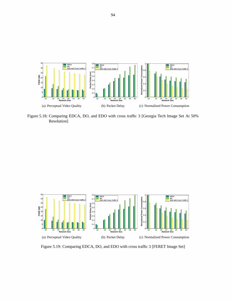
94

10 16 20 24 28 32 36 400

5

10

15

20

25

30

35

PS

NR

(dB

)

Network Size

EDCA DO EDO with Cross Traffic 3


10 16 20 24 28 32 36 400

0.1

0.2

0.3

0.4

0.5

0.6

0.7

0.8

Pac

ket D

elay

(se

c)

Network Size


(b) Packet Delay

10 16 20 24 28 32 36 400

0.2

0.4

0.6

0.8

1

Nor

mal

ized

Pow

er C

onsu

mpt

ion

Network Size



Figure 5.18: Comparing EDCA, DO, and EDO with cross traffic 3 [Georgia Tech Image Set At 50%Resolution]

10 16 20 24 28 32 36 400

5

10

15

20

25

30

35

40

PS

NR

(dB

)

Network Size



10 16 20 24 28 32 36 400

0.1

0.2

0.3

0.4

0.5

0.6

0.7

0.8

Pac

ket D

elay

(se

c)

Network Size


(b) Packet Delay

10 16 20 24 28 32 36 400

0.2

0.4

0.6

0.8

1

Nor

mal

ized

Pow

er C

onsu

mpt

ion

Network Size



Figure 5.19: Comparing EDCA, DO, and EDO with cross traffic 3 [FERET Image Set]

95

CHAPTER 6

ACCURACY-BASED CROSS-LAYER OPTIMIZATION FORAUTOMATED VIDEO SURVEILLANCE

6.1 Introduction

In this chapter, the main idea is to formulate the bandwidth allocation problem as a cross-layer

optimization problem of the sum of the weighted event detection accuracy (oralternatively the sum of

the weighted detection error), subject to the constraint in the total available bandwidth. The weights can

be assigned based on many factors, including the potential threat level, placement of video sources, and

location importance. Therefore, the weights represent the importance levels of various video sources

at the current time. With this formulation, we show that the problem can be solved using Lagrangian

relaxation techniques. The solution employs rate-accuracy curves (i.e. accuracy functions of the rate

or bandwidth), which are best to be generated for each video source inits designated location. The

proposed solution considers three layers: Application, Link, and Physical.

The main contributions of this part of the dissertation can be summarized as follows. (1) We propose

a complete accuracy-based cross-layer optimization solution. Up to our knowledge, this is the first cross-

layer solution that optimizes the detection accuracy in AVS systems. (2) The proposed solution utilizes a

novelProportional Integral Differential(PID) controller algorithm for estimating the effective airtime of

the wireless medium. (3) We develop an accurate model that characterizes the relationship between the

video data rate and the face detection accuracy error. (4) We proposea bandwidth pruning mechanism

that can be used to achieve the desired power consumption and detection accuracy tradeoff.

We evaluate the proposed solution by streaming real MJPEG video frames (and not just an abstract

bit stream) and MPEG-4 video streams over a simulated network. The simulationsare conducted using

OPNET. Since the sent video packets may be lost, we implement an error concealment algorithm [71]

at the proxy station to mitigate the impact of packet loss on video quality. The results show that the

96

proposed framework enhances the accuracy of face detection appliedon the received video streams and

yields a significant power reduction and that the new proposed effective airtime estimation algorithm is

accurate and converges quickly.

The rest of this chapter is organized as follows. Section 6.2 presents the proposed accuracy-based

cross-layer optimization framework. Section 6.3 discusses the performance evaluation methodology.

Finally, Section 6.4 presents and analyzes the main results.

6.2 Proposed Accuracy-Based Cross-Layer Optimization Framework

In this study, we consider an automated video surveillance (AVS) system, in which multiple video

sources/stations (cameras and/or sensors) stream videos to a central station over a single-hop IEEE

802.11 WLAN network in the EDCA mode. The main two challenges in the considered system can

be summarized as follows.(1) The wireless network has limited available bandwidth, which should be

estimated accurately and distributed efficiently among various video sourcesto maximize the detection

accuracy of the computer vision algorithm(s) running on the proxy station.(2) Providing differen-

tial bandwidth assignment to different sources is required because various sources in the network have

different characteristics, including channel conditions, power constraints, and lighting conditions. In

addition, different sources may have different importance levels. As shown in Figure 1.2, the system has

S ≥ 1 video sources and each sources streams a different encoded video at rateRs. Each video source

s may have a different physical rate (ys) and importance level or weight (ws). The weight represents

the importance level of a video source at the current time and depends on many factors, including the

potential threat level, placement of video sources, and location importance. In this study, we assume

that the weights are already predetermined.

The ultimate objective of this study is to provide an optimal solution that dynamically distributes and

allocates the available network bandwidth among various video sources. This solution should consider

all system, video, network, and environmental aspects, which may changedynamically. Therefore, the

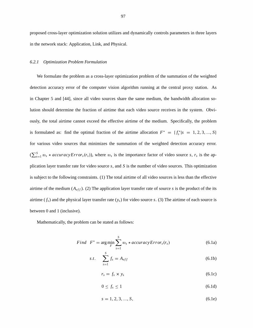
97

proposed cross-layer optimization solution utilizes and dynamically controls parameters in three layers

in the network stack: Application, Link, and Physical.

6.2.1 Optimization Problem Formulation

We formulate the problem as a cross-layer optimization problem of the summation of the weighted

detection accuracy error of the computer vision algorithm running at the central proxy station. As

in Chapter 5 and [44], since all video sources share the same medium, the bandwidth allocation so-

lution should determine the fraction of airtime that each video source receives in the system. Obvi-

ously, the total airtime cannot exceed the effective airtime of the medium. Specifically, the problem

is formulated as: find the optimal fraction of the airtime allocationF∗ = { f ∗s |s = 1, 2, 3, ..., S}

for various video sources that minimizes the summation of the weighted detection accuracy error.

(∑S

s=1 ws ∗ accuracyErrors(rs)), wherews is the importance factor of video sources, rs is the ap-

plication layer transfer rate for video sources, andS is the number of video sources. This optimization

is subject to the following constraints. (1) The total airtime of all video sources is less than the effective

airtime of the medium (Aef f ). (2) The application layer transfer rate of sources is the product of the its

airtime (fs) and the physical layer transfer rate (ys) for video sources. (3) The airtime of each source is

between 0 and 1 (inclusive).

Mathematically, the problem can be stated as follows:

Find F∗ = arg minF

S∑

s=1

ws ∗ accuracyErrors(rs) (6.1a)

s.t.S

∑

s=1

fs = Aef f (6.1b)

rs = fs × ys (6.1c)

0 ≤ fs ≤ 1 (6.1d)

s = 1, 2, 3, ..., S, (6.1e)

98

whereF∗ is the set of optimal fractions (f ∗s ) of the airtime of all sources,r ∗

s is the optimal application-

layer rate of video sources, ys is the physical-layer rate of video sources, andAef f is the total effective

airtime.

To solve the problem formulated in Equation (6.1), we need to characterize the accuracy error func-

tion and assess the effective airtime of the network.

6.2.2 Rate-Accuracy Characterization

We seek to find a model of the relationship between the playback rate of a video and the accuracy

error of a computer vision algorithm applied to the video. To keep the study focused, we analyze only

the face detection algorithm. Experimenting with other computer vision algorithms is left for another

study. We use the Viola-Jones algorithm for face detection as implemented in OpenCV. In this study, we

characterize the rate-accuracy relationship of two video compression standards: MJPEG and MPEG-4.

MJPEG Rate-Accuracy Characterization

We determine the MJPEG size-accuracy error relationship based on the following image datasets:

CMU/MIT [72], Georgia Tech [73], and SCFace [75]. We use these image sets in our experiments to

assemble the MJPEG video streams using the streamer discussed in Section 6.3 toload the network with

video traffic. For fair evaluations of bandwidth allocation solutions, each video source should be able

to stream the video at a bitrate that matches that of the optimization solution. The Georgia Tech image

set produces a highly limited range of bitrates for the studied network. To produce a better variety, we

generate two image sets from the original Georgia Tech image set by changing the resolution of each

image in the set to 30% and 50% of the original resolution, respectively. Thenew image sets have

resolutions of 192×144 and 320×240, respectively. Using these sets, the video sources can achieve the

rates produced by the optimization more accurately. In SCFace, the images are taken by three cameras

at three different distances from the subjects. Effectively, the cameras capture different resolutions of

99

the subjects. We refer to these image sets in decreasing order of the distance asSCFace at Distance 1,

SCFace at Distance 2, andSCFace at Distance 3.

For each image set, we use the IJG JPEG library to compress each picture in theset with quality

factors from 1 to 100, with 1 being the lowest, and then apply the computer vision algorithm on each

image to calculate the accuracy using a predefined ground truth about the location of the faces in the

image. We use two metrics for the detection accuracy:positive indexandnegative index. The positive

index is determined asx/y, assuming the image containsy faces and the algorithm detectsx faces

correctly. In contrast, the negative index is determined asz/y, wherez faces are detected but do not exist

in the image. We can then find the average size, the average positive index,and the average negative

index of all images with the same quality factor and then the accuracy error can be calculated as the sum

of the total error:accuracyError= (1 − posit iveIndex) + negativeIndex. The results are shown

in Figure 6.1. By curve fitting the results, we determine that the accuracy error can be characterized as

follows:

accuracyError= a × Zb + c, (6.2)

whereZ is the image size anda,b, andc are constants. This model is referred to as “Model” in Figure

6.1. For MJPEG videos, image sizeZ can be calculated asZ = R/τ , whereR is the video playback

rate andτ is the video frame rate.

MPEG-4 Rate-Accuracy Characterization

We use theYUV Video Sequencesfrom [80] to characterize the MPEG-4 Rate-Accuracy relation-

ship. In particular, we use the video sequences Akiyo, Carphone, Claire, Foreman, Grandma, Miss

America, Mother and Daughter, News, Salesman, Silent, and Suzie for QCIF resolution characteriza-

tion and we use Foreman, Mother and Daughter, News, and Silent video sequences for CIF resolution

characterization. We started by generating a ground truth for the position of the faces in each frame

100

of each video sequence. After that, we useFFmpeglibrary and the option-qscaleto compress each

video with quality scales from 2 to 31, with 2 being the highest quality, and then apply the computer

vision algorithm on each video frame to calculate the accuracy using the ground truth that we generated

initially. We use two metrics for the detection accuracy:positive indexandnegative index. The posi-

tive index is determined asx/y, assuming the video containsy faces and the algorithm detectsx faces

correctly. In contrast, the negative index is determined asz/y, wherez faces are detected but do not

exist in the video. We can then find the average frame size per video sequence and then we can find

the average frame size, the average positive index, and the average negative index of all videos with the

same quality factor and resolution and then the accuracy error can be calculated as the sum of the total

error:accuracyError= (1 − posit iveIndex) + negativeIndex.

For comparative purposes, we also perform rate-distortion characterization on the MPEG-4 se-

quences. We followed the same approach as with rate-accuracy characterization. We assess the dis-

tortion of each video frame against the uncompressed video frame using theRoot Mean Square Error

(RMSE) metric. The video distortion can then be calculated as the average frame distortion of all the

frames in the video.

The results are shown in Figure 6.2. By curve fitting the results, we determinethat the MPEG-4

accuracy error and distortion can be characterized using the following model:

Model = a × Zb + c, (6.3)

whereZ is the average video frame size anda,b, andc are constants. For any MPEG-4 videos, average

frame sizeZ can be calculated asZ = R/τ , whereR is the video playback rate andτ is the video frame

rate. This model is referred to as “Model” in Figure 6.2.

101

6.2.3 Effective Airtime Estimation

As finding an accurate value for the effective airtime of the medium is necessary for solving the

formulated optimization problem, we propose a new online and dynamic effective airtime estimation

algorithm for wireless networks in infrastructure configuration. In contrast with existing analytical mod-

els, the online approach uses complete information about the network and involves the cooperation of

the access point and all video sources as well as various layers in eachsource. To yield an accurate

estimation, the proposed approach computes the effective airtime when the packet loss in the network is

below a specified threshold.

The proposed algorithm is based on the approach that we proposed in Chapter 5 but uses aPropor-

tional Integral Differential(PID) controller for adjusting the currently estimated value of the effective

airtime in order to achieve a faster, more stable, and more accurate estimation. As depicted in Figure

6.3, the PID controller adjusts the current effective airtime value based onthe history and the rate of

change of the error. The error depends on the dropping rate in the network. The PID controller has

three components:proportional, integral, anddifferential. These components are weighted by constants

K P, K I andKD, respectively. The proportional component changes the effective airtime based on the

immediate value of the error. The integral component considers the past values of the error, whereas the

differential component anticipates the future, and thus they help reduce the steady state error and the

overshoot, respectively.

As shown in Figure 6.4, the new estimation algorithm proceeds as follows. First, for each video

sources, it finds the throughput (ts) of its video stream as received by the application layer of the

proxy station, when all sources stream videos, each at a rate that is equal to the maximum physical

rate of the network divided by the number of sources [77]. The algorithmthen uses these throughput

values to determine the initial value of the effective airtime (Aef f ) as follows: Aef f =∑S

s=1 ts/ys. Our

experiments indicate that this initial value significantly overestimates the effective airtime, causing the

102

actual received video rates to not conform to the cross-layer optimizationsolution because of the high

level of packet dropping in the network. Thus, this value has to be adjusted based on the experienced

level of packet dropping. Subsequently, during a period of time, called estimation period, each video

sources assesses its own data dropping rate (ds) while sending its video stream, and then sends this

information to the access point (AP). Meanwhile, the AP determines the overall average dropping ratio

as follows:A1 =∑S

s=1 ds/ys. The PID error is than calculated asAthresh− A1 andAef f is adjusted by

the PID controller to eliminate the error as illustrated in Figure 6.3.

We use the following well-established procedure in control theory to tune thethree PID parameters.

(1) SetK I andKD to zeros and increaseK P until the output oscillates, and then setK P to half of that

value. (2) IncreaseK I until any offset is corrected in adequate time. (3) IncreaseKD until the reference

can be reached quickly after load disturbance.

6.2.4 Optimization Solution

Now that we have an accuracy error function (which is the same for both MJPEG and MPEG-4) and

a value for the effective airtime, we can solve the problem formulated in Equation (6.1). The problem

solution can be summarized as follows:

Step 1: We first prove that the formulated problem is a convex programming problemby determining

that all constraints ((6.1b)-(6.1e)) in the problem are linear and thus convex and that the optimization

function∑S

s=1(ws(as( fsys/τ)bs + cs)) is also convex. The latter is valid since the derivative of the sum

term is monotonically non-decreasing and convex.

Step 2:Since the problem is a budget constrained convex programming problem, it can be solved using

the Lagrangian relaxation technique [78]. Thus, we can write the followingLagrangian-relaxed formula:

L(F∗, λ) =

S∑

s=1

(ws(as( fsys/τs)bs + cs)) + λ(

S∑

s=1

fs − Aef f ), (6.4)

103

where 0≤ fs ≤ 1, ands = 1, 2, 3, ..., S. Next, the Lagrangian conditions are formulated as follows:

∂L

∂ fs= 0 and

∂L

∂λ= 0. (6.5)

Assuming that all video sources have the samebs, which is empirically valid, solving these two equations

yields the following solution:

f ∗s = (

−λ∗τs

wsasbsys(ys/τs)(bs−1))(1/(bs−1)), (6.6)

where

λ∗ = (Aef f

∑Ss=1(

−τswSasbsys(ys/τs)(bs−1) )

(1/(bs−1)))(bs−1). (6.7)

6.2.5 The Allocation Algorithm

With the aforementioned solution, the access point (AP) determinesλ∗ and sends it to all video

sources in the network using the beacon packet. When a video sources receivesλ∗, it determines its

fraction of the airtimef ∗s and it changes the application data rate, which is the video encoding rate in

this case, according to the equation:r ∗s = f ∗

s × ys. Finally, the link-layer parameters are determined

based on the allocated airtime for each source. The link-layer parameters can either be the transmission

opportunity duration limit (TXOP limit) or alternatively the frequency of the transmission opportunity.

The control of the TXOP limit is more preferred since it is only one parameter,whereas the transmission

frequency involves three parameters (AIFS,CWmin, andCWmax), which complicates the control process

design. We used the model proposed in Chapter 5 to determine the TXOP limit.

104

6.2.6 Proposed Bandwidth Pruning Mechanism

As discussed earlier, with the optimization solution, each video source can determine its sending

application rate. The results in Figure 6.1 suggest that the detection accuracy increases only slightly with

the video rate (application rate) after a certain point. (That point varies based on the system, network,

and environmental conditions.) Therefore, we propose abandwidth pruningmechanism to achieve any

desired tradeoff between the detection accuracy and power consumption. With this mechanism, each

video source adjusts (reduces) its application rate if the anticipated loss in thedetection accuracy is below

a certain threshold. The threshold can be simply a fixed percentage or a function of the remaining battery

energy in the video source and its importance. The pruning mechanism is of significant importance,

especially when the sources are battery operated.

In this study, we experiment with 4 levels of bandwidth pruning: 95%, 90%, 80%, and 70%. Each

level specifies the percentage of the original accuracy that will be achieved after the pruning mechanism

is applied. Level 95%, for example, means that the achieved detection accuracy for each video source

after pruning will be 95% of that produced by the optimization solution. In other words, a 5% reduction

in the accuracy will be experienced by each source. Obviously, with higher reductions in the bandwidth,

greater savings in power consumption will be achieved.

6.3 Performance Evaluation Methodology

We use OPNET to evaluate the effectiveness of the proposed optimization solution, including the

effective airtime estimation algorithm and the bandwidth pruning mechanism.

We use two types of video traffic in our evaluation: MJPEG and MPEG-4. For MJPEG, we use the

video streamer described in Section 5.3. In the case of MPEG-4, we implemented a video streamer that

takes a video playback rate and a frame rate and produces raw video packets to simulate a video stream.

We experimented with QCIF as well as CIF video resolutions.

105

We also used similar experiment setups as in Section 5.3 and Table 6.1 summarizesthe main simu-

lation parameters.

Table 6.1: Summary of Simulation ParametersParameter Model/Value(s)Number of video sources 4-68Simulation Time 10 minPacket Size 1024 bytesApplication Rate Optimized, Default = Max Physical Rate / No. of SourcesVideo Frame Rate 20 frames/secPhysical characteristics Extended Rate (802.11g)Physical Data Rate Random from{12Mb/s, 18Mb/s, 24Mb/s, 36Mb/s, 48Mb/s, 54Mb/s}

Weight One of five levels between [0 1] chosen randomlyBuffer size 256 KbVideo TXOP limit Optimized, Default = 3008µsVideoCWmin 15VideoCWmax 31Video AIFS 2Short Retry Limit 7Long Retry Limit 4Beacon Interval 0.02 secondState Report Interval 1 second

We compare the proposed accuracy-based optimization solution, referred to in the results asWeighted

Accuracy Optimization(WAO), with the following two solutions.

• The cross-layer solution in Chapter 5, calledEnhanced Distortion Optimization(EDO).

• A new version of EDO that uses weights for various video sources, which is referred to here as

Weighted Distortion Optimization(WDO).

We analyze the followingperformance metrics.

• Weighted Accuracy- It is the sum of the weighted detection accuracy of each video source. The

accuracy for each source is found as the average accuracy of the received frames sent by that source.

The accuracy of a dropped video frame is assumed to be 0.

• Overall Network Load- It is defined as the total load sent by the application layers of all video

sources.

• Power Consumption- It is the average power consumption of the wireless interfaces of the video

106

sources and is determined by using the power consumption model in [79].


Using the aforementioned manual tuning method and extensive experimentation, we observe that

the best values for the PID parameters depend on the workload and the desired value ofAthresh. Table

6.2 summarizes these results.

Table 6.2: Summary of PID Parameter TuningWorkload Athresh K P K I KD

Georgia Tech at 30% Resolution0.001 1 0.25 0.25Georgia Tech at 30% Resolution0.005 1.5 0.25 0.25Georgia Tech at 50% Resolution0.001 0.5 0.25 0.25Georgia Tech at 50% Resolution0.005 1.5 0.25 0.25CMU/MIT 0.005 0.5 0.25 0.25MPEG-4 QCIF Resolution 0.005 1.5 0.25 0.25MPEG-4 CIF Resolution 0.005 1.5 0.25 0.25

6.4.1 Effectiveness of the Proposed Effective Airtime Estimation

Let us start by showing the effectiveness of the proposed effectiveairtime estimation algorithm

utilizing the PID controller in terms of convergence time and stability. Figure 6.5 shows the output

effective airtime values over time for Georgia Tech at 30% and 50% of the original resolution. The results

demonstrate that the PID estimator is fast to converge to a stable state and has very small overshooting

and undershooting.

Figure 6.6 shows the average effective airtime versus the number of videosources for the three

bandwidth allocation solutions. These results show that the effective airtime increases with the network

size up to a point and then starts to decrease. The peak happens when theproper balance between node

contention and network utilization is reached. The peak point in the figure is when the network size is

16, but this value varies with the total sending rate of the sources. In particular, the peak should happen

at a smaller network size if the sources are more demanding for bandwidth and at a larger network size

if the sources are less demanding. Note that the three solution yield close airtimes, especially for larger

107

networks.

Let us now discuss the impact ofAthresh, which determines the allowable packet dropping in the

network, on the weighted accuracy metric and power consumption. Figure 6.7 shows the results of

running the proposed WAO solution for two different network sizes. Theresults demonstrate that the

weighted accuracy metric improves withAthresh up to a point and then starts to worsen. The peak

happens whenAthresh is smaller than 0.01, suggesting that that optimal accuracy is achieved when the

dropping is very small. As expected, the power consumption increases withAthresh because the sending

rate increases withAthresh. Therefore,Athresh should be selected based on the proper tradeoff between

accuracy and power consumption. According to the figure, the value thatcauses the peak in accuracy

could be chosen.

6.4.2 Effectiveness of the Proposed Bandwidth Allocation Solution

Figures 6.8 and 6.9 compare the performance of various solutions (EDO, WAO, WDO) for Athresh

values of 0.001 and 0.005, respectively, when using Georgia Tech dataset at 30% resolution. Figure

6.10 shows the same results whenAthresh is equal to 0.005 and for Georgia Tech at 50% resolution.

Furthermore, Figure 6.11 shows the results for CMU/MIT dataset andAthresh = 0.005. Moreover,

Figures 6.12 and 6.13 show the same results for MPEG-4 QCIF and CIF resolutions respectively when

Athresh = 0.005.

These results show that the proposed accuracy-based optimization solution (WAO) outperforms other

solutions in all metrics. In particular, it improves both the weighted accuracy and power consumption

by up to 10%. The improvement in power consumption is due to reducing the application rates (network

loads) of various video sources. In addition, the results indicate that incorporating weights for various

video sources with the distortion-based optimization has no noticeable improvement. On the contrary, it

may worsen the weighted accuracy in some cases. By carefully analyzing these results, we noticed that

applying these weights in WDO forces the video sources with low importance factors to send the video

108

streams at extremely low bitrates, and in some cases, it prevents these sources from sending any video,

leading to an unacceptable levels of accuracy for these sources.

6.4.3 Effectiveness of the Proposed Bandwidth Pruning Mechanism

Figures 6.14-6.16 show the effectiveness of the bandwidth pruning mechanism in terms of weighted

accuracy, overall network load, and power consumption for various image datasets and values ofAthresh.

Furthermore, Figure 6.17 shows the same results for MPEG-4 CIF resolution when Athresh = 0.005.

Not all combinations are shown since the shown results are representative of the overall behavior. The

results demonstrate that the effectiveness of pruning when the WAO solution is used. Four levels of

pruning are analyzed: 95%, 90%, 80%, and 70%, with each level specifying the percentage of the

original accuracy that will be achieved after the pruning mechanism is applied. The result shows that the

pruning mechanism significantly reduces the overall network load and power consumption with much

less reduction in the weighted detection accuracy. For example, with 95% pruning, we can save up to

45% in power consumption by scarifying only 5% in the accuracy.

Finally, let us discuss the effectiveness of the proposed WAO solution withthe pruning mechanism,

compared with the other two solutions (EDO and WDO). Figures 6.18 and 6.19 compare EDO, WDO,

and WAO to WAO with 95% pruning in terms of weighted accuracy, overall network load, and power

consumption forAthresh of 0.005 and two different datasets. (The results for other datasets and values

of Athresh exhibit similar behavior.) The results demonstrate that while the WAO solution with 95%

pruning achieves almost the same values of weighted accuracy as EDO andWDO, it yields up to 45%

saving in power consumption and network load.

6.5 Conclusions

We have proposed an accuracy-based cross-layer video optimization framework for automated video

surveillance systems that manages the network bandwidth to minimize the sum of theweighted detec-

109

tion accuracy in video streams. The proposed framework utilizes an enhanced effective airtime esti-

mation algorithm utilizing aProportional Integral Differential(PID) controller. Moreover, we have

proposed a bandwidth pruning mechanism to achieve any desired tradeoff between detection accuracy

and power consumption. Furthermore, we have developed an accurate model for characterizing the

rate-accuracy relationship. We have evaluated our framework by streaming real video frames over an

OPNET-simulated wireless network.

The main results can be summarized as follows. (1) The proposed framework significantly enhances

both the detection accuracy and power consumption, compared to the distortion-based optimization. The

reduction in power consumption is due to sending and dropping much less data. (2) The proposed PID-

based effective airtime estimation algorithm is accurate, converges quickly,and more stable than the

one proposed in Chapter 5. (3) With a 95% pruning level, the proposed bandwidth allocation solution

achieves almost the same accuracy as the distortion-based optimization but reduces power consumption

by up to 45%.

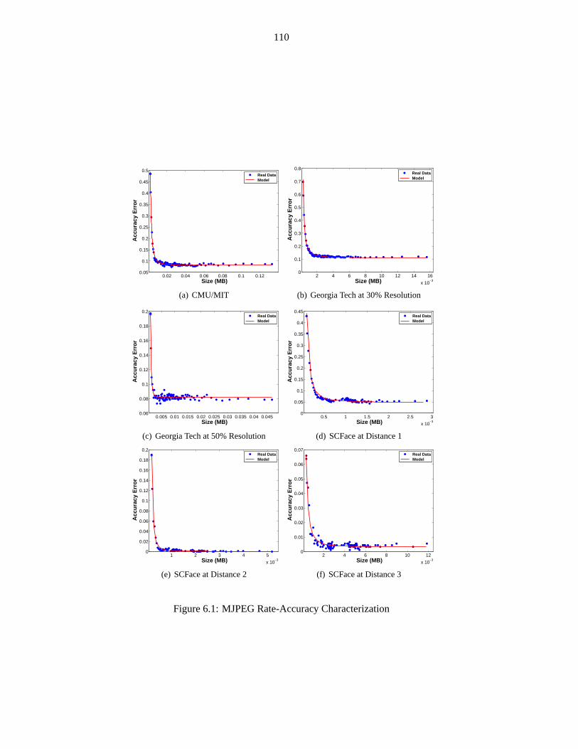
110

0.02 0.04 0.06 0.08 0.1 0.120.05

0.1

0.15

0.2

0.25

0.3

0.35

0.4

0.45

0.5

Acc

urac

y E

rror

Size (MB)

Real Data Model

(a) CMU/MIT

2 4 6 8 10 12 14 16

x 10−3

0

0.1

0.2

0.3

0.4

0.5

0.6

0.7

0.8

Acc

urac

y E

rror

Size (MB)

Real Data Model

(b) Georgia Tech at 30% Resolution

0.005 0.01 0.015 0.02 0.025 0.03 0.035 0.04 0.0450.06

0.08

0.1

0.12

0.14

0.16

0.18

0.2

Acc

urac

y E

rror

Size (MB)

Real Data Model

(c) Georgia Tech at 50% Resolution

0.5 1 1.5 2 2.5 3

x 10−3

0

0.05

0.1

0.15

0.2

0.25

0.3

0.35

0.4

0.45

Acc

urac

y E

rror

Size (MB)

Real Data Model

(d) SCFace at Distance 1

1 2 3 4 5

x 10−3

0

0.02

0.04

0.06

0.08

0.1

0.12

0.14

0.16

0.18

0.2

Acc

urac

y E

rror

Size (MB)

Real Data Model

(e) SCFace at Distance 2

2 4 6 8 10 12

x 10−3

0

0.01

0.02

0.03

0.04

0.05

0.06

0.07

Acc

urac

y E

rror

Size (MB)

Real Data Model

(f) SCFace at Distance 3

Figure 6.1: MJPEG Rate-Accuracy Characterization

111

0.5 1 1.5 2 2.5

x 10−3

0.24

0.26

0.28

0.3

0.32

0.34

0.36

0.38

0.4

0.42

0.44

Acc

urac

y E

rror

Size (MB)

Real Data Model

(a) Size-Accuracy, QCIF

2 4 6 8 10

x 10−3

0.18

0.19

0.2

0.21

0.22

0.23

0.24

0.25

0.26

0.27

0.28

Acc

urac

y E

rror

Size (MB)

Real Data Model

(b) Size-Accuracy, CIF

0.5 1 1.5 2 2.5

x 10−3

2

4

6

8

10

12

14

16

Dis

tort

ion

(RM

SE

)

Size (MB)

Real Data Model

(c) Size-Distortion, QCIF

2 4 6 8 10

x 10−3

3

4

5

6

7

8

9

10

11

12

13

Dis

tort

ion

(RM

SE

)

Size (MB)

Real Data Model

(d) Size-Distortion, CIF

Figure 6.2: MPEG-4 Rate-Accuracy and Rate-Distortion Characterization

Figure 6.3: Simplified PID Controller for Effective Airtime Estimation

while initialization period is not expiredForce each source to send in a rate equals to themaximum physical rate divided by the number of sources;Updatets value for each source.

Aef f =∑S

s=1 ts/ys;At the end of each estimation period{

A1 =∑S

s=1 ds/ys;BeforeLastError=LastError;LastError=error;error = Athresh− A1;Aef f = Aef f + K P × error − K I × Last Error + KD ×

Bef oreLast Error;}

Figure 6.4: Simplified PID Algorithm for Dynamically Estimating the Effective Airtime

112

0 100 200 300 400 5000.15

0.2

0.25

0.3

0.35

0.4

0.45

0.5

0.55

Effe

ctiv

e A

irtim

e

Time (s)

32 Stations


48 Stations


36 Stations

(a) Georgia Tech at 30% Resolution,Athresh= 0.005

0 100 200 300 400 5000.1

0.2

0.3

0.4

0.5

0.6

Effe

ctiv

e A

irtim

e

Time (s)

16 Stations

24 Stations

28 Stations

32 Stations

36 Stations

40 Stations

(b) Georgia Tech at 50% Resolution,Athresh = 0.005

Figure 6.5: Effectiveness of Proposed PID-Based Estimation

0 10 20 30 40 50 600.2

0.25

0.3

0.35

0.4

0.45

0.5

0.55

Effe

ctiv

e A

irtim

e

Network Size

EDO WDO WAO

Figure 6.6: ComparingVarious Band-width AllocationSolutions inEffective Airtime[Georgia Tech at30% Resolution,Athresh = 0.005]

0 0.005 0.01 0.0150.74

0.75

0.76

0.77

0.78

0.79

0.8

Wei

ghte

d A

ccur

acy

Athresh

52 Sources 56 Sources

(a) Weighted Accuracy

0 0.005 0.01 0.0150.75

0.8

0.85

0.9

0.95

1

Nor

mal

ized

Pow

er C

onsu

mpt

ion

Athresh

52 Sources 56 Sources

(b) Power Consumption

Figure 6.7: Impact ofAthresh with Proposed Weighted Accuracy Optimization [Georgia Tech at 30%Resolution]

35 40 45 50 55 60 65

0.65

0.7

0.75

0.8

Wei

ghte

d A

ccur

acy

Network Size

EDO WDO WAO


35 40 45 50 55 60 656

7

8

9

10

11

12x 10

6

Ove

rall

Net

wor

k Lo

ad R

ate

(bps

)

Network Size

EDO WDO WAO

(b) Overall Network Load

35 40 45 50 55 60 650.55

0.6

0.65

0.7

0.75

0.8

0.85

0.9

0.95

Nor

mal

ized

Pow

er C

onsu

mpt

ion

Network Size

EDO WDO WAO

(c) Power Consumption

Figure 6.8: Comparing the Effectiveness of Various Bandwidth Allocation Solutions [Georgia Tech at30% Resolution,Athresh = 0.001]

113

35 40 45 50 55 60 650.66

0.68

0.7

0.72

0.74

0.76

0.78

0.8

Wei

ghte

d A

ccur

acy

Network Size

EDO WDO WAO


35 40 45 50 55 60 650.7

0.8

0.9

1

1.1

1.2

1.3x 10

7

Ove

rall

Net

wor

k Lo

ad R

ate

(bps

)

Network Size

EDO WDO WAO


35 40 45 50 55 60 650.5

0.6

0.7

0.8

0.9

1

Nor

mal

ized

Pow

er C

onsu

mpt

ion

Network Size

EDO WDO WAO


Figure 6.9: Comparing the Effectiveness of Various Bandwidth Allocation Solutions [Georgia Tech at30% Resolution,Athresh = 0.005]

25 30 35 400.81

0.82

0.83

0.84

0.85

0.86

Wei

ghte

d A

ccur

acy

Network Size

EDO WDO WAO


25 30 35 400.7

0.8

0.9

1

1.1

1.2

1.3x 10

7

Ove

rall

Net

wor

k Lo

ad R

ate

(bps

)

Network Size

EDO WDO WAO


25 30 35 400.55

0.6

0.65

0.7

0.75

0.8

0.85

0.9

0.95

Nor

mal

ized

Pow

er C

onsu

mpt

ion

Network Size

EDO WDO WAO


Figure 6.10: Comparing the Effectiveness of Various Bandwidth AllocationSolutions [Georgia Tech at50% ResolutionAthresh = 0.001]

16 18 20 22 24 26 280.5

0.55

0.6

0.65

0.7

0.75

Wei

ghte

d A

ccur

acy

Network Size

EDO WDO WAO


16 18 20 22 24 26 281.1

1.2

1.3

1.4

1.5

1.6

1.7

1.8

1.9x 10

7

Ove

rall

Net

wor

k Lo

ad R

ate

(bps

)

Network Size

EDO WDO WAO


16 18 20 22 24 26 280.5

0.6

0.7

0.8

0.9

1

Nor

mal

ized

Pow

er C

onsu

mpt

ion

Network Size

EDO WDO WAO


Figure 6.11: Comparing the Effectiveness of Various Bandwidth AllocationSolutions [CMU/MIT,Athresh = 0.005]

114

20 22 24 26 28 30 320.68

0.69

0.7

0.71

0.72

0.73

0.74

0.75

Wei

ghte

d A

ccur

acy

Network Size

EDO WDO WAO


20 22 24 26 28 30 321.25

1.3

1.35

1.4

1.45

1.5

1.55x 10

7

Ove

rall

Net

wor

k Lo

ad R

ate

(bps

)

Network Size

EDO WDO WAO


20 22 24 26 28 30 320.55

0.6

0.65

0.7

0.75

0.8

0.85

0.9

0.95

Nor

mal

ized

Pow

er C

onsu

mpt

ion

Network Size

EDO WDO WAO


Figure 6.12: Comparing the Effectiveness of Various Bandwidth AllocationSolutions [MPEG-4 QCIFResolution,Athresh = 0.005]

20 22 24 26 28 30 320.74

0.75

0.76

0.77

0.78

0.79

0.8

0.81

0.82

Wei

ghte

d A

ccur

acy

Network Size

EDO WDO WAO


20 22 24 26 28 30 321.25

1.3

1.35

1.4

1.45

1.5

1.55x 10

7

Ove

rall

Net

wor

k Lo

ad R

ate

(bps

)

Network Size

EDO WDO WAO


20 22 24 26 28 30 320.55

0.6

0.65

0.7

0.75

0.8

0.85

0.9

0.95

Nor

mal

ized

Pow

er C

onsu

mpt

ion

Network Size

EDO WDO WAO


Figure 6.13: Comparing the Effectiveness of Various Bandwidth AllocationSolutions [MPEG-4 CIFResolution,Athresh = 0.005]

35 40 45 50 55 60 65

0.5

0.6

0.7

0.8

0.9

Wei

ghte

d A

ccur

acy

Network Size

WAO without Pruning WAO with 95% Pruning WAO with 90% Pruning WAO with 80% Pruning WAO with 70% Pruning


35 40 45 50 55 60 652

4

6

8

10

12x 10

6

Ove

rall

Net

wor

k Lo

ad R

ate

(bps

)

Network Size



35 40 45 50 55 60 650.4

0.5

0.6

0.7

0.8

0.9

1

Nor

mal

ized

Pow

er C

onsu

mpt

ion

Network Size



Figure 6.14: Effectiveness of Bandwidth Pruning Mechanism [WAO Solution, Georgia Tech at 30%Resolution,Athresh = 0.005]

115

28 30 32 34 36 38 400.76

0.78

0.8

0.82

0.84

0.86

Wei

ghte

d A

ccur

acy

Network Size



28 30 32 34 36 38 404

5

6

7

8

9

10

11

12

x 106

Ove

rall

Net

wor

k Lo

ad R

ate

(bps

)

Network Size



28 30 32 34 36 38 400.5

0.6

0.7

0.8

0.9

1

Nor

mal

ized

Pow

er C

onsu

mpt

ion

Network Size



Figure 6.15: Effectiveness of Bandwidth Pruning Mechanism [WAO Solution, Georgia Tech at 50%Resolution,Athresh = 0.005]

16 18 20 22 24 26 280.5

0.55

0.6

0.65

0.7

0.75

Wei

ghte

d A

ccur

acy

Network Size



16 18 20 22 24 26 280.6

0.8

1

1.2

1.4

1.6

1.8x 10

7

Ove

rall

Net

wor

k Lo

ad R

ate

(bps

)

Network Size



16 18 20 22 24 26 280.5

0.6

0.7

0.8

0.9

1

Nor

mal

ized

Pow

er C

onsu

mpt

ion

Network Size



Figure 6.16: Effectiveness of Bandwidth Pruning Mechanism [WAO Solution, CMU/MIT, Athresh =

0.005]

20 22 24 26 28 30 320.55

0.6

0.65

0.7

0.75

0.8

0.85

0.9

Wei

ghte

d A

ccur

acy

Network Size



20 22 24 26 28 30 320

5

10

15x 10

6

Ove

rall

Net

wor

k Lo

ad R

ate

(bps

)

Network Size



20 22 24 26 28 30 320.5

0.6

0.7

0.8

0.9

1

Nor

mal

ized

Pow

er C

onsu

mpt

ion

Network Size



Figure 6.17: Effectiveness of Bandwidth Pruning Mechanism [WAO Solution, MPEG-4 CIF Resolution,Athresh = 0.005]

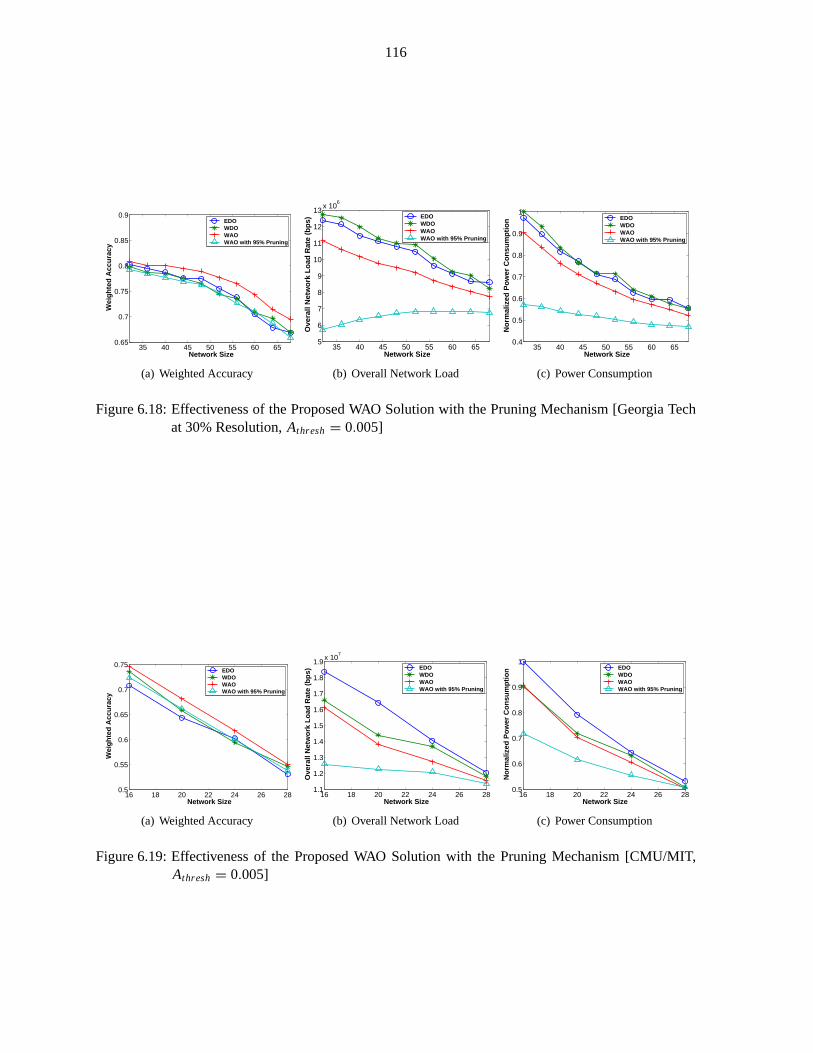
116

35 40 45 50 55 60 650.65

0.7

0.75

0.8

0.85

0.9

Wei

ghte

d A

ccur

acy

Network Size

EDO WDO WAO WAO with 95% Pruning


35 40 45 50 55 60 655

6

7

8

9

10

11

12

13x 10

6

Ove

rall

Net

wor

k Lo

ad R

ate

(bps

)

Network Size



35 40 45 50 55 60 650.4

0.5

0.6

0.7

0.8

0.9

1

Nor

mal

ized

Pow

er C

onsu

mpt

ion

Network Size



Figure 6.18: Effectiveness of the Proposed WAO Solution with the PruningMechanism [Georgia Techat 30% Resolution,Athresh = 0.005]

16 18 20 22 24 26 280.5

0.55

0.6

0.65

0.7

0.75

Wei

ghte

d A

ccur

acy

Network Size



16 18 20 22 24 26 281.1

1.2

1.3

1.4

1.5

1.6

1.7

1.8

1.9x 10

7

Ove

rall

Net

wor

k Lo

ad R

ate

(bps

)

Network Size



16 18 20 22 24 26 280.5

0.6

0.7

0.8

0.9

1

Nor

mal

ized

Pow

er C

onsu

mpt

ion

Network Size



Figure 6.19: Effectiveness of the Proposed WAO Solution with the PruningMechanism [CMU/MIT,Athresh = 0.005]

117

CHAPTER 7

SUMMARY AND FUTURE WORK

7.1 Summary

7.1.1 Waiting-time Predictability

We have analyzed the waiting-time predictability in scalable video streaming and have presented

two prediction schemes:Assign Expected Stream Completion Time(AEC) andHybrid Prediction. AEC

utilizes detailed information about the server state and considers the applied scheduling policy to predict

the future scheduling decisions over a certain period, calledprediction window. This window introduces

a tradeoff between the prediction accuracy and the number of users receiving expected waiting times.

The hybrid scheme uses AEC and then assigns the average video waiting time for those requests that did

not obtain a predicted time by AEC.

We have analyzed the effectiveness of the two prediction schemes when applied with various stream

merging techniques and scheduling policies. We have also compared the effectiveness of the waiting-

time prediction approach with the approach that provides time-of-service guarantees. The latter is rep-

resented by an extended policy, calledGeneralized Next Schedule Time First(GNSTF). In addition, we

have studied the impacts of prediction window, server capacity, user’s waiting tolerance, arrival rate,

skew in video access, video length, and number of videos.


• The waiting time can be predicted accurately, especially with AEC and when MCF-P is used. MCF-

P is not only highly predictable (in terms of user waiting time) but also achieves the best performance

in server throughput and average waiting time.

• In contrast with AEC, the hybrid prediction scheme provides expected times toeach user but achieves

lower accuracy and a longer confidence interval.

118

• Combining AEC or the hybrid scheme with MCF-P leads to outstanding performance benefits, com-

pared with GNSTF.

• This combination, calledPredictive MCF-P, can be applied with hierarchical stream merging tech-

niques (such as ERMT) to improve performance further, whereas GNSTF cannot.

7.1.2 Scheduling

We have analyzed in detail cost-based scheduling for on-demand video streaming and proposed new

strategies:Predictive Cost-Based Scheduling(PCS) andAdaptive Regular Stream Triggering(ART).


• There is no clear advantage of computing the cost over a future time window, compared with com-

puting the cost only at the next scheduling time.

• The proposed PCS scheduling policy outperforms the best existing policy (MCF-P) in terms of

customer defection probability and average waiting time. The waiting times can alsobe predicted

more accurately with PCS. The two variations of PCS (PCS-V and PCS-L) perform nearly the same

and thus the simpler variant (PCS-V) is preferred because of its lower implementation complexity.

• By enhancing stream merging behavior, the proposed ART technique substantially improves both

the customer defection probability and the average waiting time.

• The best overall performer is “MCF-P combined with ART”, followed by PCS. With ART, signifi-

cantly more clients can receive expected waiting times for service than PCS, but at a somewhat lower

waiting time accuracy.

7.1.3 Distortion-based Dynamic Bandwidth Allocation

We have proposed a cross-layer video optimization framework that manages the network bandwidth

to minimize the total distortion in video streams. The proposed framework utilizes a new online network

effective airtime estimation algorithm. Moreover, we have developed a new and accurate model for

119

characterizing the video data rate and distortion relationship as well as a newmodel for adapting the link-

layer parameters. We have evaluated our framework by streaming real video frames over an OPNET-

simulated wireless network.


• The proposed framework enhances substantially the perceptual quality of received video streams.

• The proposed effective airtime estimation algorithm is accurate and converges quickly.

• Optimal perceptual video quality is achieved when the packet dropping is very small.

• The transmission opportunity adaptation model works effectively.

• The proposed framework results in much less power consumption, compared with existing solutions.

This behavior is due to sending and dropping much less data. Power consumption is a primary

concern, especially when the video sources are battery-powered.

• The proposed framework is highly adaptable to any interfering traffic in thenetwork.

7.1.4 Accuracy-based Dynamic Bandwidth Allocation

We have proposed an accuracy-based cross-layer video optimization framework for automated video

surveillance systems that manages the network bandwidth to minimize the sum of theweighted detec-

tion accuracy in video streams. The proposed framework utilizes an enhanced effective airtime esti-

mation algorithm utilizing aProportional Integral Differential(PID) controller. Moreover, we have

proposed a bandwidth pruning mechanism to achieve any desired tradeoff between detection accuracy

and power consumption. Furthermore, we have developed an accurate model for characterizing the

rate-accuracy relationship. We have evaluated our framework by streaming real video frames over an

OPNET-simulated wireless network.


• The proposed framework significantly enhances both the detection accuracy and power consump-

120

tion, compared to the distortion-based optimization. The reduction in power consumption is due to

sending and dropping much less data.

• The PID-based effective airtime estimation algorithm is accurate and more stable than the one pro-

posed in Chapter 5.

• With pruning, the proposed bandwidth allocation solution achieves almost the same accuracy as the

distortion-based optimization but reduces power consumption significantly.

7.2 Future Work

In future work, we plan to study the cross-layer framework with more computer vision algorithms,

such as face recognition and object tracking. We also plan to study the framework with different video

adaptation techniques, including resolution-based adaptation. Furthermore, we plan to perform study

with different networks, such as WiMAX.

BIBLIOGRAPHY

[1] “Alexa The Web Information Company,” http://www.alexa.com/topsites.

[2] Brandon C Welsh and David P Farrington, “Evidence-based crime prevention: The effectiveness of

cctv,” Crime Prevention and Community Safety An International Journal, vol. 6, no. 2, pp. 21–33,

2004.

[3] “CCTV Image 42: How many cameras are there in the UK?,”

http://www.securitynewsdesk.com/wp-content/uploads/2011/03/CCTV-Image-42-How-many-

cameras-are-there-in-the-UK.pdf.

[4] “Chicago’s video surveillance cameras: A pervasive and unregulated threat to our privacy,”

2011, http://heartland.org/policy-documents/chicagos-video-surveillance-cameras-pervasive-and-

unregulated-threat-our-privacy.

[5] Isaac Wang, “China video surveillance revenue to reach $9.5 billion by 2014,” 2011,

http://www.isuppli.com/China-Electronics-Supply-Chain/MarketWatch/Pages/China-Video-

Surveillance-Revenue-to-Reach-$95-Billion-by-2014.aspx.

[6] Kien A. Hua, Ying Cai, and Simon Sheu, “Patching: A multicast technique for true Video-on-

Demand services,” inProc. of ACM Multimedia, 1998, pp. 191–200.

[7] Ying Cai and Kien A. Hua, “An efficient bandwidth-sharing technique for true video on demand

systems,” inProc. of ACM Multimedia, Oct. 1999, pp. 211–214.

[8] D. L. Eager, M. K. Vernon, and J. Zahorjan, “Optimal and efficient merging schedules for Video-

on-Demand servers,” inProc. of ACM Multimedia, Oct. 1999, pp. 199–202.

[9] Marcus Rocha, Marcelo Maia, Italo Cunha, Jussara Almeida, and Sergio Campos, “Scalable media

streaming to interactive users,” inProc. of ACM Multimedia, Nov. 2005, pp. 966–975.

121

122

[10] Huadong Ma, G. Kang Shin, and Weibiao Wu, “Best-effort patching for multicast true VoD ser-

vice,” Multimedia Tools Appl., vol. 26, no. 1, pp. 101–122, 2005.

[11] Bashar Qudah and Nabil J. Sarhan, “Towards scalable delivery of video streams to heterogeneous

receivers,” inProc. of ACM Multimedia, Oct. 2006, pp. 347–356.

[12] Musab Al-Hadrusi and Nabil J. Sarhan, “A scalable delivery framework and a pricing model

for streaming media with advertisements,” inProc. of SPIE/ACM Multimedia Computing and

Networking Conference (MMCN), Januray 2008.

[13] K. A. Hua and S. Sheu, “Skyscraper broadcasting: A new broadcasting scheme for metropolitan

Video-on-Demand system,” inProc. of ACM SIGCOMM, Sept. 1997, pp. 89–100.

[14] L. Juhn and L. Tseng, “Harmonic broadcasting for Video-on-Demand service,”IEEE Trans. on

Broadcasting, vol. 43, no. 3, pp. 268–271, Sept. 1997.

[15] J.-F. Paris, S. W. Carter, and D. D. E. Long, “Efficient broadcasting protocols for video on demand,”

in Proc. of the Int’l Symp. on Modeling, Analysis and Simulation of Computerand Telecommuni-

cation Systems (MASCOTS), July 1998, pp. 127–132.

[16] Cheng Huang, Ramaprabhu Janakiraman, and Lihao Xu, “Loss-resilient on-demand media stream-

ing using priority encoding,” inProc. of ACM Multimedia, Oct. 2004, pp. 152–159.

[17] Liqi Shi, Phillipa Sessini, Anirban Mahanti, Zongpeng Li, and Derek L. Eager, “Scalable streaming

for heterogeneous clients,” inProc. of ACM Multimedia, Oct. 2006, pp. 337–346.

[18] S. W. Carter and D. D. E. Long, “Improving Video-on-Demand server efficiency through stream

tapping,” in the International Conference on Computer Communication and Networks (ICCCN),

Sept. 1997, pp. 200–207.

123

[19] Y. Cai and Kien A. Hua, “Sharing multicast videos using patching streams,”Multimedia Tools and

Applications journal, vol. 21, no. 2, pp. 125–146, Nov. 2003.

[20] Y. Cai, W. Tavanapong, and Kien A. Hua, “Enhancing patching performance through double

patching,” inProc. of 9th Intl Conf. on Distributed Multimedia Systems, Sept. 2003, pp. 72–77.

[21] D. L. Eager, M. K. Vernon, and J. Zahorjan, “Bandwidth skimming:A technique for cost-effective

Video-on-Demand,” inProc. of Multimedia Computing and Networking Conf. (MMCN), Jan. 2000,

pp. 206–215.

[22] Nabil J. Sarhan and Bashar Qudah, “Efficient cost-based scheduling for scalable media streaming,”

in Proc. of Multimedia Computing and Networking Conf. (MMCN), January 2007.

[23] Robert Collins, Alan Lipton, Takeo Kanade, Hironobu Fujiyoshi, David Duggins, Yanghai Tsin,

David Tolliver, Nobuyoshi Enomoto, and Osamu Hasegawa, “A system for video surveillance

and monitoring,” Tech. Rep. CMU-RI-TR-00-12, Robotics Institute, Carnegie Mellon University,

Pittsburgh, PA, May 2000.

[24] Omar Javed and Mubarak Shah, “Tracking and object classification for automated surveillance,”

in Proceedings of the 7th European Conference on Computer Vision-PartIV, 2002, pp. 343–357.

[25] Xiaojing Yuan, Zehang Sun, Yaakov Varol, and George Bebis, “Adistributed visual surveillance

system,” inProceedings of the IEEE Conference on Advanced Video and Signal Based Surveillance

(AVSS), 2003, p. 199.

[26] Lun Zhang, Stan Z. Li, Xiaotong Yuan, and Shiming Xiang, “Real-time object classification in

video surveillance based on appearance learning,” inCVPR, 2007.

[27] Artur oza, Lyudmila Mihaylova, David Bull, and Nishan Canagarajah,“Structural similarity-based

object tracking in multimodality surveillance videos,”Mach. Vision Appl., vol. 20, no. 2, pp. 71–83,

Jan. 2009.

124

[28] Yangqing Jia and Changshui Zhang, “Front-view vehicle detectionby markov chain monte carlo

method,”Pattern Recognition, vol. 42, no. 3, pp. 313–321, 2009.

[29] Lubomir Bourdev, Subhransu Maji, and Jitendra Malik, “Describingpeople: Poselet-based at-

tribute classification,” inInternational Conference on Computer Vision (ICCV), 2011.

[30] V. Nair and J. Clark, “Automated visual surveillance using hidden markov models,” inProceedings

of the 15th International Conference on Vision Interface (VI), May 2002, pp. 88–92.

[31] W. Niu and J. Long, “Human activity detection and recognition for video surveillance,” inPro-

ceedings of the IEEE Multimedia and Expo Conference (ICME), June 2004, pp. 719–722.

[32] Yi githan Dedeoglu, B. Ugur Toreyin, Ugur Gudukbay, and A. Enis Cetin, “Silhouette-based

method for object classification and human action recognition in video,” inProceedings of the

2006 international conference on Computer Vision in Human-Computer Interaction, Berlin, Hei-

delberg, 2006, ECCV’06, pp. 64–77, Springer-Verlag.

[33] Rajat Singh, Sarvesh Vishwakarma, Anupam Agrawal, and M. D. Tiwari, “Unusual activity de-

tection for video surveillance,” inProceedings of the First International Conference on Intelligent

Interactive Technologies and Multimedia, New York, NY, USA, 2010, IITM ’10, pp. 297–305,

ACM.

[34] Juan Carlos Niebles, Chih-Wei Chen, , and Li Fei-Fei, “Modeling temporal structure of decompos-

able motion segments for activity classification,” inProceedings of the 12th European Conference

of Computer Vision (ECCV), Crete, Greece, September 2010.

[35] L. Fei-Fei and L.-J. Li, “What, Where and Who? Telling the Story of an Image by Activity Clas-

sification, Scene Recognition and Object Categorization,”Studies in Computational Intelligence-

Computer Vision, pp. 157–171, 2010.

125

[36] Wu-Chi Feng, Ed Kaiser, Wu Chang Feng, and Mikael Le Baillif, “Panoptes: scalable low-power

video sensor networking technologies,”ACM Trans. Multimedia Comput. Commun. Appl., vol. 1,

no. 2, pp. 151–167, 2005.

[37] Xiaoan Lu, Elza Erkip, Yao Wang, and David Goodman, “Power efficient multimedia communi-

cation over wireless channels,”IEEE Journal on Selected Areas in Communications, vol. 21, pp.

1738–1751, 2003.

[38] Zhihai He and Dapeng Wu, “Resource allocation and performanceanalysis of wireless video

sensors,”IEEE Transactions on Circuits and Systems for Video Technology, vol. 16, pp. 590–599,

2006.

[39] Y. Andreopoulos, N. Mastronarde, and M. van der Schaar, “Cross-Layer Optimized Video Stream-

ing Over Wireless Multihop Mesh Networks,”Selected Areas in Communications, IEEE Journal

on, vol. 24, no. 11, pp. 2104–2115, 2006.

[40] S. Khan, J. Brehmer, W. Kellerer, W. Utschick, and E. Steinbach,“Application-driven cross-layer

optimization for video streaming over wireless networks,”IEEE Communications Magazine, vol.

44, pp. 122–130, 2006.

[41] Honghai Zhang, Yanyan Zheng, Mohammad Ali Khojastepour, andSampath Rangarajan, “Cross-

layer optimization for streaming scalable video over fading wireless networks,” IEEE Journal on

Selected Areas in Communications, vol. 28, no. 3, pp. 344–353, 2010.

[42] Mihaela van der Schaar, Yiannis Andreopoulos, and Zhiping Hu, “Optimized scalable video

streaming over ieee 802.11a/e hcca wireless networks under delay constraints,” IEEE Transac-

tions on Mobile Computing, vol. 5, pp. 755–768, June 2006.

126

[43] Jian wei Huang, Zhu Li, Mung Chiang, and Aggelos K. Katsaggelos, “Pricing-based rate con-

trol and joint packet scheduling for multi-user wireless uplink video streaming,” in Proc. 15th

International Packet Video Workshop (PV2006), 2006.

[44] Cheng-Hsin Hsu and Mohamed Hefeeda, “A framework for cross-layer optimization of video

streaming in wireless networks,” 2011.

[45] Pavel Korshunov and Wei Tsang Ooi, “Critical video quality for distributed automated video

surveillance,” inProceedings of the 13th annual ACM international conference on Multimedia,

2005, pp. 151–160.

[46] Pavel Korshunov, “Rate-accuracy tradeoff in automated, distributed video surveillance systems,” in

Proceedings of the 14th annual ACM international conference on Multimedia, 2006, pp. 887–889.

[47] Pavel Korshunov and Wei Tsang Ooi, “Video quality for face detection, recognition, and tracking,”

ACM Trans. Multimedia Comput. Commun. Appl., vol. 7, no. 3, pp. 14:1–14:21, Sept. 2011.

[48] D. L. Eager, M. K. Vernon, and J. Zahorjan, “Minimizing bandwidthrequirements for on-demand

data delivery,” IEEE Trans. on Knowledge and Data Engineering, vol. 13, no. 5, pp. 742–757,

Sept. 2001.

[49] A. Bar-Noy, G. Goshi, R.E. Ladner, and K. Tam, “Comparison of stream merging algorithms for

Media-on-Demand,”Multimedia Systems Journal, vol. 9, pp. 211–223, 2004.

[50] A. Dan, D. Sitaram, and P. Shahabuddin, “Scheduling policies for an on-demand video server with

batching,” inProc. of ACM Multimedia, Oct. 1994, pp. 391–398.

[51] C. C. Aggarwal, J. L. Wolf, and P. S. Yu, “The maximum factor queue length batching scheme for

Video-on-Demand systems,”IEEE Trans. on Computers, vol. 50, no. 2, pp. 97–110, Feb. 2001.

127

[52] Nabil J. Sarhan and Chita R. Das, “A new class of scheduling policies for providing time of

service guarantees in Video-On-Demand servers,” inProc. of the 7th IFIP/IEEE Int’l Conf. on

Management of Multimedia Networks and Services, Oct. 2004, pp. 127–139.

[53] N.S. Shankar and M. van der Schaar, “Performance analysis ofvideo transmission over ieee

802.11a/e wlans,”IEEE Transactions on Vehicular Technology, vol. 56, no. 4, pp. 2346 –2362,

july 2007.

[54] Ye Ge, Jennifer C. Hou, and Sunghyun Choi, “An analytic study oftuning systems parameters

in ieee 802.11e enhanced distributed channel access,”Computer Networks, vol. 51, no. 8, pp.

1955–1980, 2007.

[55] Chun-Ting Chou, S. N. Shankar, and Kang G. Shin, “Achieving per-stream qos with distributed

airtime allocation and admission control in ieee 802.11e wireless lans,” inINFOCOM, 2005, pp.

1584–1595.

[56] I. Pavlidis, V. Morellas, P. Tsiamyrtzis, and S. Harp, “Urban surveillance systems: From the

laboratory to the commercial world,”IEEE Proceedings, vol. 89, no. 10, pp. 1478–1497, October

2001.

[57] O. Javed, Z. Rasheed, O. Alatas, and M. Shah, “KNIGHT: A real-time surveillance system for mul-

tiple overlapping and non-overlapping cameras,” inProceedings of IEEE International Conference

on Multimedia and Expo (ICME), July 2003, pp. 649–652.

[58] R. Rangaswami, Z. Dimitrijevi, K. Kakligian, E. Chang, and Y. Wang, “The SfinX video surveil-

lance system,” inProceedings of the IEEE International Conference on Multimedia and Expo

(ICME), June 2004.

[59] Jie Hui and M. Devetsikiotis, “A unified model for the performance analysis of IEEE 802.11e

EDCA,” Communications, IEEE Transactions on, vol. 53, no. 9, pp. 1498–1510, 2005.

128

[60] Lixiang Xiong and Guoqiang Mao, “Saturated throughput analysis of ieee 802.11e edca,”Com-

puter Networks, vol. 51, no. 11, pp. 3047–3068, 2007.

[61] Zhenyu Yang and Klara Nahrstedt, “A bandwidth management framework for wireless camera

array,” inNOSSDAV, 2005, pp. 147–152.

[62] Samarth H. Shah, Kai Chen, and Klara Nahrstedt, “Dynamic bandwidth management in single-hop

ad hoc wireless networks,”MONET, vol. 10, no. 1-2, pp. 199–217, 2005.

[63] Samarth H. Shah, Kai Chen, Klara Nahrstedt, and I. Introduction,“Available bandwidth estimation

in ieee 802.11-based wireless networks,” 2003.

[64] Cheikh Sarr, Claude Chaudet, Guillaume Chelius, and Isabelle GuerinLassous, “Bandwidth es-

timation for ieee 802.11-based ad hoc networks,”IEEE Trans. Mob. Comput., vol. 7, no. 10, pp.

1228–1241, 2008.

[65] Nabil J. Sarhan and Chita R. Das, “A new class of scheduling policies for providing time of

service guarantees in Video-On-Demand servers,” inProc. of the 7th IFIP/IEEE Int’l Conf. on

Management of Multimedia Networks and Services, Oct. 2004, pp. 127–139.

[66] A. K. Tsiolis and M. K. Vernon., “Group-guaranteed channel capacity in multimedia storage

servers.,” inProc. of ACM SIGMETRICS, June 1997, pp. 285–297.

[67] C. Costa, I. Cunha, A. Borges, C. Ramos, M. Rocha, J. Almeida, and B. Ribeiro-Neto, “Analyzing

client interactivity in streaming media,” inProc. of The World Wide Web Conf., May 2004, pp.

534–543.

[68] Cristiano Costa, Italo Cunha, Alex Borges, Claudiney Ramos, Marcus Rocha, Jussara Almeida,

and Berthier Ribeiro-neto, “Analyzing client interactivity in streaming media,”2004.

129

[69] I. Ari, B. Hong, E. Miller, S. Brandt, and D. Long, “Managing flash crowds on the internet,” in

Proc. of the 11th IEEE/ACM International Symposium on Modeling, Analysis, and Simulation of

Computer and Telecommunication Systems (MASCOTS), Oct. 2003, pp. 246–249.

[70] Bashar Qudah and Nabil J. Sarhan, “Analysis of resource sharing and cache management tech-

niques in scalable video-on-demand,” inProc. of the 14th IEEE International Symposium on

Modeling, Analysis, and Simulation of Computer and Telecommunication Systems (MASCOTS),

Sept. 2006, pp. 327–334.

[71] Shahram Shirani, Faouzi Kossentini, Samir Kallel, and Rabab Ward,“Reconstruction of jpeg

coded images in lossy packet networks,” .

[72] “CMU/MIT image set,” http://vasc.ri.cmu.edu/idb/html/face/frontalimages.

[73] “Georgia tech face database,” http://www.anefian.com/research/face reco.htm.

[74] P. Jonathon Phillips, Harry Wechsler, Jeffrey Huang, and Patrick J. Rauss, “The FERET database

and evaluation procedure for face-recognition algorithms,”Image Vision Comput., vol. 16, no. 5,

pp. 295–306, 1998.

[75] Mislav Grgic, Kresimir Delac, and Sonja Grgic, “Scface - surveillance cameras face database,”

Multimedia Tools Appl., vol. 51, no. 3, pp. 863–879, 2011.

[76] Wenye Cheng, Xi Chen, and Zhihai He, “Doubling of the operational lifetime of portable video

communication devices using power-rate-distortion analysis and control,” inICIP, 2006, pp. 2473–

2476.

[77] Andrew Symington and Pieter S. Kritzinger, “A hardware test bed for measuring ieee 802.11g

distribution coordination function performance,” inMASCOTS, 2009, pp. 1–7.

130

[78] A Ortega and K Ramchandran, “Rate-distortion methods for image and video compression,”IEEE

Signal Processing Magazine, vol. 15, no. 6, pp. 23–50, 1998.

[79] Yousef Sharrab and Nabil J. Sarhan, “Aggregate power consumption modeling of live video stream-

ing systems,” inACM Multimedia Systems (MMSys 2013), Oslo, Norway, February 2013.

[80] “Yuv video sequences,” http://trace.eas.asu.edu/yuv/index.html.

131

ABSTRACT

MAXIMIZING RESOURCE UTILIZATION IN VIDEO STREAMING SYSTEMS

by

MOHAMMAD ABDULLAH ALSMIRAT

May 2013

Advisor: Dr. Nabil Sarhan

Major : Computer Engineering

Degree: Doctor of Philosophy

Video streaming has recently grown dramatically in popularity over the Internet, Cable TV, and wireless

networks. Because of the resource demanding nature of video streamingapplications, maximizing re-

source utilization in any video streaming system is a key factor to increase the scalability and decrease

the cost of the system. Resources to utilize include server bandwidth, network bandwidth, battery life

in battery operated devices, and processing time in limited processing power devices. In this work, we

propose new techniques to maximize the utilization of video-on-demand (VOD) server resources. In

addition to that, we propose new framework to maximize the utilization of the networkbandwidth in

wireless video streaming systems.

Providing video streaming users in a VOD system with expected waiting times enhances their per-

ceived quality-of-service (QoS) and encourages them to wait therebyincreasing server utilization by

increasing server throughput. In this work, we analyze waiting-time predictability in scalable video

streaming. We also propose two prediction schemes and study their effectiveness when applied with

various stream merging techniques and scheduling policies. The results demonstrate that the waiting

time can be predicted accurately, especially when enhanced cost-based scheduling is applied. The com-

bination of waiting-time prediction and cost-based scheduling leads to outstanding performance bene-

fits. The achieved resource sharing by stream merging depends greatlyon how the waiting requests are

scheduled for service. Motivated by the development of cost-based scheduling, we investigate its effec-

132

tiveness in great detail and discuss opportunities for further tunings and enhancements. Additionally,

we analyze the effectiveness of incorporating video prediction results into the scheduling decisions. We

also study the interaction between scheduling policies and the stream merging techniques and explore

new ways for enhancements.

The interest in video surveillance systems has grown dramatically during the last decade. Auto-

mated video surveillance (AVS) serves as an efficient approach for therealtime detection of threats and

for monitoring their progress. Wireless networks in AVS systems have limited available bandwidth that

have to be estimated accurately and distributed efficiently. In this research,we develop two cross-layer

optimization frameworks that maximize the bandwidth optimization of 802.11 wireless network. We

develop a distortion-based cross-layer optimization framework that manages bandwidth in the wire-

less network in such a way that minimizes the overall distortion. We also developan accuracy-based

cross-layer optimization framework in which the overall detection accuracyof the computer vision al-

gorithm(s) running in the system is maximized. Both proposed frameworks manage the application

rates and transmission opportunities of various video sources based on the dynamic network conditions

to achieve their goals. Each framework utilizes a novel online approach for estimating the effective

airtime of the network. Moreover, we propose a bandwidth pruning mechanism that can be used with

the accuracy-based framework to achieve any desired tradeoff between detection accuracy and power

consumption. We demonstrate the effectiveness of the proposed frameworks, including the effective air-

time estimation algorithms and the bandwidth pruning mechanism, through extensiveexperiments using

OPNET.

133

AUTOBIOGRAPHICAL STATEMENT

Mohammad Alsmirat received his Bachelor’s degree in Computer Science in 2002 from Jordan

University of Science and Technology and received his Master’s degree in Computer Science from New

York Institute of Technology in 2003. Mohammad joined the department of Electrical and Computer

Engineering (ECE) at Wayne State University to pursue his PhD degree inComputer Engineering in

January, 2007 and he is currently a PhD. candidate. He has previouslyworked as full time lecturer in

the Computer Science department at Jordan University of Science and Technology from October, 2003

until December, 2006. In January, 2007, he started working as Graduate Research Assistant in the ECE

department at Wayne State University and then he started to work as Graduate Teaching Assistant in the

ECE department in August, 2007 until December 2012. Mohammad started to work at General Motors

Research and Development center in January 2013 to do research in Vehicle to Vehicle Communication

area.

Maximizing Resource Utilization In Video Streaming Systems

Documents

Transcript of Maximizing Resource Utilization In Video Streaming Systems