Modeling Viewer and Influencer Behavior on Streaming Platforms

by

Prashant Rajaram

A dissertation submitted in partial fulfillment

of the requirements for the degree of

Doctor of Philosophy

(Business Administration)

in The University of Michigan

2021

Doctoral Committee:

Professor Puneet Manchanda, Chair

Assistant Professor David Jurgens

Associate Professor Jun Li

Associate Professor Eric M. Schwartz

Prashant Rajaram

prajaram@umich.edu

ORCID iD: 0000-0002-8638-3772

© Prashant Rajaram 2021

ii

DEDICATION

This dissertation is dedicated to my wife, Ankita Deepkumar,

for her continuous support, encouragement and love.

iii

ACKNOWLEDGMENTS

I am very grateful to the wonderful people at the University of Michigan who I have had the fortune of

meeting during the PhD Program which has truly been a transformative experience. I am grateful to the

selection committee responsible for making me an offer to join the program and giving me the

opportunity to learn and grow in a wonderful academic environment. I would like to extend my sincere

gratitude to Puneet Manchanda, for taking me on as his PhD student, and mentoring me over the course of

six years. His mentorship approach of “tough love” has served me well, pushed me to achieve more and

helped me experience joy in research. He has always encouraged constructive debates and has always

been willing to explore new ideas. Meetings spent discussing and debating about research aspects with

him for three hours straight have been some of the highlights of my PhD experience! They have taught

me how to think logically and analytically, and have shaped me as a researcher. His genuine care and

concern about my well-being in the program have always been an added source of comfort. Puneet’s

mentorship approach has been complemented well by that of Eric Schwartz, to whom I am also very

grateful. His hands-on and patient approach to mentorship, and his help in breaking down complex ideas

into simple parts helped me learn so much. Moreover, his frequent words of encouragement have always

instilled confidence in me. One of the main reasons I joined the program was for the opportunity to work

with Eric on the topic of binge-watching, and I am grateful to him for helping make that dream come true.

I am very grateful to David Jurgens for offering valuable insights and suggestions on my research

and for his support during the job market. I would also like to thank Jun Li for being generous with her

time and for her helpful feedback on my research. I am very grateful to S. Sriram for being a reassuring

voice in the Marketing PhD committee, for always providing constructive feedback on my progress, for

providing valuable feedback on my research, and for his support during the job market. I am also grateful

to Anocha Aribarg, Rajeev Batra, Fred Feinberg, Aradhna Krishna, Yesim Orhun, Scott Rick, David

Wooten, Katherine Burson, Carolyn Yoon, Justin Huang, and Jessica Fong for offering valuable feedback

on my research at various stages of the program. I would also like to thank Fred Feinberg for teaching a

fantastic PhD course by leading all paper discussions, and I would also like to thank Carolyn Yoon and

Scott Rick for being very kind and supportive PhD Coordinators. My time in the program has been

enriched by several interactions I have had with faculty from departments outside Marketing, and I would

iv

like to thank them all. I would like to especially thank Brisa Sanchez for being a fantastic teacher and

engaging in several discussions after class.

I am very grateful to the wonderful students I met from 2015 to 2021 across various schools and

departments including the Marketing PhD program at Ross. I would like to especially thank Mike

Palazollo and Linda Hagen for making me feel very welcomed when I joined the program, Kanzheng Zhu

and Huanyu Zheng for their generous help and support with coursework, Longxiu Tian for his very kind

and generous mentorship, Dan Zhao and Aseem Sinha for their kindness and support, Xu Zhang for

always helping me with my questions, Tong Guo for providing valuable feedback on my research,

Rebecca Chae for her generous help with teaching, and Gwen Ahn for engaging in helpful conversations

about research. In addition, I would also like to thank Tim Doering, Dana Turjeman, Tiffany Vu, Steve

Shaw, Yiqi Li, Yu Song, Hayoung Cheon, Adithya Pattabhiramaiah, Harsh Ketkar, Jihoon Cho, Giacomo

Meille, Mengzhenyu Zhang, Jiawei Li, Jangwon Choi, Varad Deolankar, Frank Li and Zoey Jiang for

providing helpful advice and feedback at various stages during the program. I would also like to sincerely

thank the administrative team at Ross – Brian Jones, Kelsey Belzak, Ashley Stauffer, Clea Davis and

Lindsay Apperson – for being very supportive and helpful.

Finally, I would like to express my gratitude to the amazing people who inspired me and

supported me in my decision to pursue a PhD – Bori Csillag for her engaging conversations that provided

the spark that research could be the way forward, Markus Giesler for his generous and kind mentorship,

for helping me realize my potential and for showing me the path ahead, and Russ Belk for being a role

model for how warm, generous, and efficient a researcher can be. While the PhD journey has generally

been filled with moments of joy and happiness, there have also been moments of challenge and doubt,

wherein I have realized that having self-belief and keeping a positive attitude always helps. I am also very

grateful to my friends Rishabh Srivastava and Neil Sheth for their consistent support, my parents, N.

Rajaram and Shyama Rajaram, for always standing with me, to my wife, Ankita Deepkumar, for her

continuous support, encouragement and love, and to my unborn child for being patient! To anyone I may

have inadvertently missed thanking, please accept my apologies, and know that you have my gratitude for

your support.

v

TABLE OF CONTENTS

DEDICATION .............................................................................................................................................. ii

ACKNOWLEDGMENTS ........................................................................................................................... iii

LIST OF TABLES ...................................................................................................................................... vii

LIST OF FIGURES ..................................................................................................................................... ix

LIST OF APPENDICES .............................................................................................................................. xi

ABSTRACT ................................................................................................................................................ xii

CHAPTER I - Introduction ........................................................................................................................... 1

CHAPTER II - Finding the Sweet Spot: Ad Scheduling on Streaming Media ............................................. 4

2.1 Introduction ......................................................................................................................................... 4

2.2 Data ..................................................................................................................................................... 7

2.2.1 Sessions ........................................................................................................................................ 8

2.2.2 Ad Delivery .................................................................................................................................. 9

2.3 Stage I ............................................................................................................................................... 10

2.3.1 Metric Development .................................................................................................................. 10

2.3.2 Data Summary via Metrics ........................................................................................................ 16

2.3.4 Metric Validity ........................................................................................................................... 16

2.4 Stage II .............................................................................................................................................. 17

2.4.1 Feature Generation ..................................................................................................................... 17

2.4.2 Model ......................................................................................................................................... 20

2.5 Results ............................................................................................................................................... 22

2.5.1 Model Estimation ....................................................................................................................... 22

2.5.2 Feature Importance .................................................................................................................... 23

2.5.3 Partial Dependence .................................................................................................................... 24

2.6 Stage III ............................................................................................................................................. 26

2.6.1 Ad Decision Tree ....................................................................................................................... 26

2.6.2 Optimization .............................................................................................................................. 27

2.6.3 Recommended Schedule: Comparison with Data ...................................................................... 30

vi

2.6.4 Decision Support System ........................................................................................................... 31

2.7 Conclusion ........................................................................................................................................ 33

2.8 Tables ................................................................................................................................................ 35

2.9 Figures .............................................................................................................................................. 42

CHAPTER III - Video Influencers: Unboxing the Mystique ..................................................................... 49

3.1 Introduction ....................................................................................................................................... 49

3.2. Related Literature ............................................................................................................................. 52

3.2.1 Influencer Marketing.................................................................................................................. 52

3.2.2 Unstructured Data Analysis in Marketing via Deep Learning ................................................... 52

3.3 Data ................................................................................................................................................... 53

3.3.1 Institutional Setting .................................................................................................................... 53

3.3.2 Video Sample ............................................................................................................................. 54

3.3.3 Outcome Variables ..................................................................................................................... 54

3.3.4 Features ...................................................................................................................................... 57

3.4. Model ............................................................................................................................................... 59

3.4.1 Text Model ................................................................................................................................. 60

3.4.2 Audio Model .............................................................................................................................. 61

3.4.3 Image Model .............................................................................................................................. 62

3.4.4 Combined Model........................................................................................................................ 63

3.5 Results ............................................................................................................................................... 63

3.5.1 Prediction Results ...................................................................................................................... 64

3.5.2 Interpretation Results ................................................................................................................. 66

3.5.3 Learning Patterns ....................................................................................................................... 74

3.5.4 Analysis Using Other Slices of Influencer Videos .................................................................... 75

3.6 Implications for Influencers and Marketers ...................................................................................... 75

3.7 Conclusion ........................................................................................................................................ 77

3.8 Tables ................................................................................................................................................ 79

3.9 Figures .............................................................................................................................................. 86

CHAPTER IV – Summary & Outlook ....................................................................................................... 94

APPENDICES ............................................................................................................................................ 96

BIBILIOGRAPHY ................................................................................................................................... 132

vii

LIST OF TABLES

Table 2.1: Summary of Sessions ......................................................................................................... 35

Table 2.2: Example timeline (in minutes) of viewing behavior in a session ...................................... 35

Table 2.3: Computation of the Bingeability Metric ............................................................................ 35

Table 2.4: Computation of the Ad Tolerance Metric .......................................................................... 35

Table 2.5: Metric Summary Statistics ................................................................................................. 36

Table 2.6a: Current Predictors ............................................................................................................ 36

Table 2.6b: Functions for watching only TV shows ........................................................................... 37

Table 2.6c: Eight features of Bingeability Sum (BS) ......................................................................... 37

Table 2.6d: Functions for watching TV shows or Movies .................................................................. 38

Table 2.7: Summary statistics for dataset used in the model .............................................................. 39

Table 2.8a: Top 10 sets of predictors of Bingeability ......................................................................... 39

Table 2.8b: Top 10 sets of predictors for Ad Tolerance ..................................................................... 39

Table 2.8c: Gain % of the Ad Targeting Rules ................................................................................... 40

Table 2.9: Recommendation Summary for Threshold, T=0 ............................................................... 40

Table 2.10a: Percent change in optimized ad exposure compared to observed ad exposure .............. 40

Table 2.10b: Percent change in optimized Bingeability compared to observed Bingeability ............ 41

Table 2.10c: Percent change in optimized Bingeability compared to initial predicted Bingeability .. 41

Table 3.1: Scraped data for videos ...................................................................................................... 79

Table 3.2: Correlation between outcomes ........................................................................................... 79

Table 3.3: Video features - structured and unstructured ..................................................................... 80

Table 3.4: Best performing model for each component of unstructured data in holdout sample ....... 80

Table 3.5: Importance of features based on the Ridge Regression Model .......................................... 81

Table 3.6: Results of the Text Regression Models ............................................................................. 81

Table 3.7: Results of the Audio Regression Models ........................................................................... 82

Table 3.8: Results of the Image Regression Models ........................................................................... 82

Table 3.9: Results from interpreting Regression Models .................................................................... 83

Table 3.10: Predictive accuracy in holdout sample using unstructured data from beginning, middle

and end of videos ................................................................................................................................ 84

Table 3.11: Score for a video outside the training sample .................................................................. 84

viii

Table 3.12: Variance explained by brand mentions ............................................................................ 85

Table A1: Different weight combinations of the components of the Ad Tolerance Metric ............. 101

Table A2: Evidence of Skipping and Excessive Fast-Forwarding .................................................... 102

Table A3: Examples of viewing behavior in a session ..................................................................... 103

Table A4: Factor Loadings from a Principal Component Analysis .................................................. 105

Table A5: Comparison of Model Performance (RMSE) on holdout sample .................................... 112

Table B1: MobileNet-v1 architecture ............................................................................................... 121

Table B2: EfficientNet-B7 architecture ............................................................................................ 123

Table B3.1: Comparison of Text Model performance in holdout sample ........................................ 126

Table B3.2: Comparison of Audio Model performance in holdout sample ...................................... 126

Table B3.3: Comparison of Thumbnail Model performance in holdout sample .............................. 127

Table B3.4: Comparison of Video Frame Model (0s,30s) performance in holdout sample ............. 127

Table B3.5: Bi-LSTM Video Frame Model (with different time intervals) ..................................... 127

Table B3.6: Performance of different Combined Models on holdout sample .................................. 128

Table B4: Results of the Text Regression Models with interactions ................................................ 130

Table B5: Results from interpreting Regression Models on middle and end of video ..................... 131

ix

LIST OF FIGURES

Figure 2.1: Three-Stage Architecture .................................................................................................. 42

Figure 2.2a: Histogram of Pod Length ................................................................................................ 42

Figure 2.2b: Histogram of Pod Spacing (min) .................................................................................... 42

Figure 2.2c: Histogram of Ad Diversity (%) ...................................................................................... 42

Figure 2.2d: Histogram of Pod Clumpiness ........................................................................................ 42

Figure 2.3a: Histogram of Bingeability .............................................................................................. 43

Figure 2.3b: Histogram of Ad Tolerance ............................................................................................ 43

Figure 2.3c: Ad Tolerance vs Bingeability ......................................................................................... 43

Figure 2.4a: Partial Dependence of Bingeability on Bingeability Sum (same Show, any Day, any

TOD) ................................................................................................................................................... 44

Figure 2.4b: Partial Dependence of Ad Tolerance on Ad Tolerance Sum (same Title, any Day, any

TOD) ................................................................................................................................................... 44

Figure 2.4c: Partial Dependence of 𝑪𝑹 on Bingeability ..................................................................... 44

Figure 2.4d: Partial Dependence of 𝑺𝑹 on Ad Tolerance ................................................................... 44

Figure 2.4e: Partial Dependence of Bingeability on its two most important Ad Targeting Rules ...... 45

Figure 2.4f: Partial Dependence of Ad Tolerance on its two most important Ad Targeting Rules .... 45

Figure 2.5: Ad Decision Tree .............................................................................................................. 46

Figure 2.6a: Density of Recommended Spacing in Holdout 1 ............................................................ 46

Figure 2.6b: Density of Recommended Spacing in Holdout 2 ........................................................... 46

Figure 2.7a: Density of Average Observed Spacing in Holdout 1 ...................................................... 47

Figure 2.7b: Density of Average Observed Spacing in Holdout 2...................................................... 47

Figure 2.8a: Density of the Ratio of Recommended Spacing and Average Observed Spacing in

Holdout 1 ............................................................................................................................................ 47

Figure 2.8b: Density of the Ratio of Recommended Spacing and Average Observed Spacing in

Holdout 2 ............................................................................................................................................ 47

Figure 2.9a: Percentage change in optimized ad exposure (𝒏) as compared to observed ad exposure

(𝒏) ....................................................................................................................................................... 48

Figure 2.9b: Percentage change in optimized Bingeability (𝒃) for Holdout 1 ................................... 48

Figure 2.9c: Percentage change in optimized Bingeability (𝒃) for Holdout 2 ................................... 48

x

Figure 3.1: Distribution of log view count .......................................................................................... 86

Figure 3.2a: Distribution of Log Engagement .................................................................................... 86

Figure 3.2b: Distribution of Log Popularity ....................................................................................... 86

Figures 3.2c: Distribution of Log Likeability ..................................................................................... 87

Figure 3.3: Distribution of average sentiment score across Top 25 comments .................................. 87

Figure 3.4a: Distribution of number of brand mentions in text .......................................................... 87

Figure 3.4b: Distribution of number of brand logos in images ........................................................... 88

Figure 3.5a Traditional Deep Learning Approach .............................................................................. 88

Figure 3.5b: Interpretable Deep Learning Approach .......................................................................... 88

Figure 3.6: BERT Model Framework ................................................................................................. 89

Figure 3.7: Audio Model ..................................................................................................................... 89

Figure 3.8: Image Model (Video Frames)........................................................................................... 90

Figure 3.9: Combined Model .............................................................................................................. 90

Figure 3.10: Interpretation strategy on holdout sample ...................................................................... 91

Figure 3.11: Attention Weights in captions/transcript (first 30s) of a video ....................................... 91

Figure 3.12: Attention weights in an audio clip (first 30s) of a video ................................................ 92

Figure 3.13: Gradient heat map (associated with engagement) in frames of a video ......................... 92

Figure 3.14: Brand Heterogeneity (brand mention in captions/transcript in first 30s vs sentiment) .. 93

Figure A1: Bingeability versus Episode Count ................................................................................. 102

Figure A2.1: Percentage change in optimized ad exposure (𝒏) as compared to observed ad exposure

(𝒏) ..................................................................................................................................................... 107

Figure A2.2: Percentage change in optimized Bingeability (𝒃) for Holdout 1 ................................ 107

Figure A2.3: Percentage change in optimized Bingeability (𝒃) for Holdout 2 ................................ 107

Figure A3.1a: Density of Naïve Spacing in Holdout 1 ..................................................................... 117

Figure A3.1b: Density of Naïve Spacing in Holdout 2 ..................................................................... 117

Figure A3.2a: Density of the Ratio of Recommended Spacing and Naïve Spacing in Holdout 1 .... 117

Figure A3.2b: Density of the Ratio of Recommended Spacing and Naïve Spacing in Holdout 2 .... 117

Figure B1: Encoders ......................................................................................................................... 119

Figure B2: Self-Attention Heads ....................................................................................................... 120

Figure B3: Bi-LSTM with Attention ................................................................................................ 122

Figure B4.1: Bi-LSTM ...................................................................................................................... 124

Figure B4.2: Max-GAP ..................................................................................................................... 124

Figure B4.3: GAP-Max ..................................................................................................................... 125

Figure B4.4: C-GAP ......................................................................................................................... 125

xi

LIST OF APPENDICES

APPENDIX A – Appendix to Chapter II .................................................................................................... 96

Appendix A.1: Details on Bingeability and Ad Tolerance ..................................................................... 96

Appendix A.2: Hulu Data Collection Methodology ............................................................................. 100

Appendix A.3: Using Different Weights in the Ad Tolerance Metric .................................................. 101

Appendix A.4: Metric Validity ............................................................................................................. 102

Appendix A.5: Modelling Correlation Between Outcomes .................................................................. 106

Appendix A.6: Tree Based Methods And Simulated Data ................................................................... 108

Appendix A.7: Cross-Validation for XGBoost ..................................................................................... 113

Appendix A.8: Optimization Procedure ................................................................................................ 114

APPENDIX B – Appendix to Chapter III ................................................................................................. 118

Appendix B.1: BERT Encoders (in Text Model).................................................................................. 118

Appendix B.2: MobileNet V1 followed by Bi-LSTM with Attention (in Audio Model) ..................... 121

Appendix B.3: EfficientNet-B7 Architecture and Combination Architectures (in Image Model) ....... 123

Appendix B.4: Comparison of Model Performance with Benchmarks ................................................ 126

Appendix B.5: Interpreting Interaction Effects in Text Model ............................................................. 129

Appendix B.6: Interpreting Results for Middle and End of Videos...................................................... 131

Appendix A.9: Recommended Schedule Versus A Naïve Heuristic .................................................... 116

xii

ABSTRACT

The video streaming industry is growing rapidly, and consumers are increasingly using ad-supported

streaming services (Graham, 2020). There are important questions related to the effect of ad schedules

and video elements on viewer behavior that have not been adequately studied in the marketing literature.

In my dissertation, I study these topics by applying causal and/or interpretable machine learning methods

on behavioral data.

In the first essay, “Finding the Sweet Spot: Ad Scheduling on Streaming Media”, I design an

“optimal” ad schedule that balances the interest of the viewer (watching content) with that of the

streaming platform (ad exposure). This is accomplished using a three-stage approach applied on a dataset

of Hulu customers. In the first stage, I develop two metrics – Bingeability and Ad Tolerance – to capture

the interplay between content consumption and ad exposure in a viewing session. Bingeability represents

the number of completely viewed unique episodes of a show, while Ad Tolerance represents the

willingness of a viewer to watch ads and subsequent content. In the second stage, I predict the value of

the metrics for the next viewing session using the tree-based machine learning method – Extreme

Gradient Boosting – while controlling for the non-randomness in ad delivery to a focal viewer using

“instrumental variables” based on ad delivery patterns to other viewers. Using “feature importance

analyses” and “partial dependence plots” I shed light on the importance and nature of the non-linear

relationship with various feature sets, going beyond a purely black-box approach. Finally, in the third

stage, I implement a novel constrained optimization procedure built around the causal predictions to

provide an “optimal” ad-schedule for a viewer, while ensuring the level of ad exposure does not exceed

her predicted Ad Tolerance. Under the optimized schedule, I find that “win-win” schedules are possible

that allow for both an increase in content consumption and ad exposure.

In the second essay, “Video Influencers: Unboxing the Mystique”, I study the relationship

between advertising content in YouTube influencer videos (across text, audio and images) and marketing

outcomes (views, interaction rates and sentiment). This is accomplished with the help of novel

interpretable deep-learning architectures that avoid making a trade-off between predictive ability and

interpretability. Specifically, I achieve high predictive performance by avoiding ex-ante feature

engineering and achieve better interpretability by eliminating spurious relationships confounded by

factors unassociated with “attention” paid to video elements. The attention mechanism in the Text and

xiii

Audio models along with gradient maps in the Image model allow identification of video elements on

which attention is paid while forming an association with an outcome. Such an ex-post analysis allows me

to find statistically significant relationships between video elements and marketing outcomes that are

supplemented by a significant increase in attention to video elements. By eliminating spurious

relationships, I generate hypotheses that are more likely to have causal effects when tested in a field

setting. For example, I find that mentioning a brand in the first 30 seconds of a video is on average

associated with a significant increase in attention to the brand but a significant decrease in sentiment

expressed towards the video.

Overall, my dissertation provides solutions and identifies strategies that can improve the welfare

of viewers, platform owners, influencers and brand partners. Policy makers also stand to gain from

understanding the power exerted by different stakeholders over viewer behavior.

1

CHAPTER I - Introduction

The video streaming industry is growing rapidly, and consumers are increasingly using ad-supported

streaming services (Graham, 2020). The on-demand aspect of streaming media allows viewers to have

increased control over the consumption experience which is different from traditional consumption

experiences on linear TV. There are important questions related to the effect of ad schedules and video

elements on viewer behavior on streaming media that have not been adequately studied in the marketing

literature. In my dissertation, I study these topics by applying causal and/or interpretable machine learning

methods on behavioral data. Specifically, in my first essay, “Finding the Sweet Spot: Ad Scheduling on

Streaming Media”, I design an “optimal” ad schedule that balances the interest of the viewer (watching

content) with that of the streaming platform (ad exposure). This is accomplished with the help of causal

and interpretable tree-based learning methods applied on a dataset of Hulu customers. In my second

essay, “Video Influencers: Unboxing the Mystique”, I study the relationship between advertising content

in YouTube influencer videos (across text, audio and images) and marketing outcomes. This is

accomplished with the help of novel interpretable deep-learning architectures that avoid making a trade-

off between predictive ability and interpretability. My approach not only predicts well out-of-sample but

also allows for interpretation of the attention paid on video elements. Next, I summarize my two essays.

Ad-scheduling on Streaming Media. Viewers consume content on streaming platforms in a self-directed

manner since these platforms, in contrast to live TV, are primarily on-demand services. On the platform

side, the tracking of individual-level viewer “eyeballs” on streaming services represents an attractive

opportunity for advertisers, especially as these services allow for ad personalization due to the availability

of rich data. However, interruptions to the viewing experience via advertising can detract from the

viewers’ feeling of being in control, potentially leading to decreased content consumption. The challenge

therefore is to balance the interests of the viewer and that of the platform while delivering advertising in

these settings. I use four months of actual viewership data from the streaming platform Hulu to propose

ad-schedules that maximize advertising exposure without compromising the content consumption

experience for individual viewers. This is accomplished using a three-stage approach.

In the first stage, I develop two metrics – Bingeability and Ad Tolerance – to capture the interplay

between content consumption and ad exposure in a viewing session. Bingeability represents the number

2

of completely viewed unique episodes of a show, while Ad Tolerance represents the willingness of a

viewer to watch ads and subsequent content. Then, I predict the value of the metrics for the next viewing

session using the tree-based machine learning method – Extreme Gradient Boosting – while controlling

for the non-randomness in ad delivery to a focal viewer using “instrumental variables” based on ad

delivery patterns to other viewers. Using “feature importance analyses” and “partial dependence plots” I

am able to shed light on the importance and nature of the non-linear relationship with various feature sets,

going beyond a purely black-box approach. Finally, I implement a novel constrained optimization

procedure built around the causal predictions to provide an “optimal” ad-schedule for a viewer, while

ensuring the level of ad exposure does not exceed her predicted Ad Tolerance. Under the optimized

schedule, I find that “win-win” schedules are possible that allow for both an increase in content

consumption and ad exposure.

Substantively, the contribution lies in using a combination of metrics, relevant data, and

optimization, to develop an advertising schedule that benefits both the viewer and the platform.

Methodologically, I demonstrate a novel implementation of tree-based machine learning in conjunction

with instrumental variables to make causal predictions. In addition, I also present an interpretable

machine learning approach that makes complex relationships between consumer behavior and managerial

actions more transparent and easier to understand.

Influencer Advertising Videos. The increasing popularity of social media influencers has resulted in an

exponential growth of the influencer marketing industry which allows brands to partner with influencers

to promote their products. The videos made by influencers differ from conventional advertising videos in

at least three ways. First, they can contain information that is unrelated to the sponsoring brand(s).

Second, they are longer in duration on average, especially on platforms such as YouTube and Instagram.

Finally, the platform often inserts conventional advertising videos into the influencer video. While there

has been ample research to study the characteristics of conventional advertising videos and their impact

on marketing outcomes, there has been little research on the design and effectiveness of influencer videos.

Using publicly available data on YouTube, I study the relationship between advertising content in

influencer videos (across text, audio, and images) and video views, interaction rates and sentiment. This is

accomplished with the help of novel interpretable deep-learning architectures that not only offer high

predictive performance by avoiding ex-ante feature engineering, but also allow interpretation of the

attention paid on unstructured influencer video elements. By supplementing the deep-learning analysis

with the benefits of transfer learning, I achieve high performance at a low computational cost.

The deep learning architectures used for analyzing each component of unstructured data in videos

are state-of the-art transfer learning methods customized for this setting. They comprise Bidirectional

3

Encoder Representation from Transformers (BERT) for textual data (title, description, and captions),

YAMNet (MobileNet) with Bidirectional Long Short-Term Memory Cells (LSTMs) appended with an

attention mechanism for audio data, and EfficientNet-B7 with Bidirectional LSTMs for image data. The

attention mechanism in the Text and Audio models along with gradient maps in the Image model allow

interpretation of the elements of videos on which attention is paid while forming an association with an

outcome. Such an ex-post analysis allows me to find statistically significant relationships between

advertising content and marketing outcomes that are supplemented by a significant increase in attention to

advertising content. I filter out relationships that are affected by confounding factors unassociated with an

increase in attention, thus generating hypotheses that are more likely to have causal effects when tested in

a field setting. For example, interpreting the results from the Text model reveals that brand mentions in

the first 30 seconds of a video are associated with a significant increase in attention to the brand but a

significant decrease in sentiment expressed towards the video. In addition, I uncover significant

relationships between sounds (e.g., speech, music, animal sounds, etc.) in audio as well as objects (e.g.,

persons, clothes, brand logos, etc.) in images with marketing outcomes that are also supplemented by an

increase in attention.

This essay uncovers novel relationships between unstructured video elements and marketing

outcomes. Influencers and brands can test these relationships for causal effects via field experiments and

build better integrated content that engenders higher viewer satisfaction with the consumption experience.

Methodologically, I introduce novel interpretable deep learning approaches to the marketing literature

that allow interpretation of the captured relationships without trading off predictive ability.

Overall, my dissertation provides solutions and identifies strategies that can improve the welfare

of viewers, platform owners, influencers and brand partners. Policy makers also stand to gain from

understanding the power exerted by different stakeholders over viewer behavior. The areas I study in my

dissertation (streaming media and influencer marketing) are growing, and the methods I use are state-of-

the-art and novel in their application to studying agent behavior in these areas.

4

CHAPTER II - Finding the Sweet Spot: Ad Scheduling on Streaming Media

2.1 Introduction

Streaming video content is becoming increasingly popular. 55% of US households subscribed to at least

one video streaming service in 2018, up from 10% in 2009 (Deloitte, 2018). In contrast to linear TV, on-

demand streaming services give viewers agency, allowing them to consume content in a self-directed

manner. As a result, viewers consume media content in a “non-linear” manner by not adhering to any set

temporal schedules. For example, a common behavior viewers exhibit in such settings is that of rapid

consumption of multiple episodes of a TV show, usually referred to as “binge-watching” (Cakebread,

2017; Oxford Dictionary 2018). The presence of consumer “eyeballs” on streaming media represents an

attractive opportunity for advertisers, especially as these services allow for ad personalization due to the

availability of rich data. As a result, advertising spending on streaming media services is expected to grow

to $20 billion in 2020 from $4.7 billion in 2017 (eMarketer, 2018).1 However, streaming media represents

new challenges, especially as interruptions to the viewing experience via advertising detract from the

viewers’ feeling of being in control and can lead to decreased content consumption (Schweidel & Moe,

2016). In addition, platforms that provide these services need to balance the viewers’ control of the

consumption experience while delivering advertising commensurate with advertiser objectives. Advertiser

objectives entail delivering a fixed number of ad exposures over a set of TV shows or movies within a

given time frame (Johnson, 2019).2 In general, there is little work that focuses on the interplay of

(consumer directed) content consumption and ad exposures. While extant research in marketing has

developed recommendations for ad scheduling, e.g., Dubé et al. (2005), the viewer does not have

significant control in the settings considered. In addition, the focus of past ad scheduling work has been

on several ad-related outcomes but not on studying content consumption.3 There is limited research that

1 Streaming media providers monetize their services through three distinct mechanisms (including offering combinations of these): subscriptions, advertising and product sales (e.g., sale of a movie). It is hard to assess which is the dominant mechanism. However, the number of ad-supported

platforms (with or without a free service) is growing rapidly with providers such as Hulu, CBS, Dailymotion, Ora TV, YouTube, Sony (Crackle),

The Roku Channel, TubiTV, Popcornflix, Amazon (IMDb TV) and NBC (Armental, 2019; Patel, 2018; Sherman, 2019). There is also industry research suggesting that consumers prefer a platform’s lower cost ad-supported streaming service to its premium no-ad version, when both options

are offered (Liyakasa, 2018; Sommerlad, 2018). In this essay, I focus on free streaming services with an ad supported mechanism. 2 My focus is on the platform’s ad scheduling problem. I do not know how the advertiser arrives at exposure targets (quantity, ad location within show, customer segment etc.) specified to the platform. I also do not have access to all the downstream data e.g., browsing, purchasing etc. 3 Recent work on ad scheduling has focused on maximizing ad-related outcomes such as profits from sales (Dubé et al., 2005), campaign reach (Danaher et al., 2010), purchase (Sahni, 2015), site visits (Chae et al., 2019) or ad viewing completion rates (Krishnan & Sitaraman, 2013).

5

has focused on content consumption patterns in settings where viewers have control, e.g., Schweidel and

Moe (2016), which does not address the ad scheduling issue.

In this essay, I propose a comprehensive approach that best combines the interests of the viewer and

that of the free ad-supported platform. Specifically, I use actual viewership data from a streaming media

platform to propose ad schedules that maximize advertising exposure without compromising the content

consumption experience for individual viewers. In order to do this, I need to surmount a few challenges.

First, the control that viewers have can manifest itself in multiple and diverse behaviors, both in

relationship to content consumption and the reaction to advertising. However, there is little

standardization on how consumer behavior on streaming media can be captured and described. Second,

there is plethora of content on streaming media platforms, varying in terms of genre, show type and show

duration (episode length, number of episodes per season and number of seasons). It becomes very

important therefore to capture the impact of these variables and their interactions in a tractable manner.

Third, in real settings, platforms do not deliver advertising randomly. Thus, any approach that is proposed

needs to address the non-random delivery of such advertising. Finally, in order for ad scheduling

recommendations to have practical value, simplicity and speed are very important.

I address these challenges using a three-stage approach (Figure 2.1). Given the lack of

standardization around the measurement of content consumption and ad exposure in streaming media

settings, I begin by using theory from consumer psychology to develop summary measures or metrics that

capture viewer’s control over the consumption experience in streaming media settings. These metrics are

deterministic transforms of the data primitives (minutes watched, ads see, etc.) that are available to

streaming media platforms. The two aspects of viewer behavior that I am interested in are non-linear

content consumption and the response to advertising exposure. In order to do this, I first need to specify a

temporal unit of consumption for a given viewer. I denote this unit as a viewer-session (in future, I use the

term “session” to denote this unit) which is defined as a period of time spent by a viewer watching one

TV show separated by 60 minutes or more of inactivity as in Schweidel and Moe (2016).

The first metric, which I label “Bingeability,” is based on the theory of “flow” (Ghani &

Deshpande, 1994; Schweidel & Moe, 2016) as well as industry norms and captures the extent of viewer

immersion in the content. In essence, this metric is based on a stylized count of complete and unique

episodes of a TV show watched in a session. The second metric, which I label “Ad Tolerance,” is based

on the theory of hedonic adaptation (Frederick & Loewenstein, 1999; Nelson et al., 2009) and captures

the viewer’s reaction to advertising. Specifically, the metric captures the willingness of a viewer to watch

ads and to watch content after being exposed to ads in a session. I explain the theoretical motivation,

construction and validation for both metrics in more detail in the section “Stage I”.

6

In the second stage, I construct a model to predict the value of the above metrics for a session using

an extensive set of current and historic descriptors, both specific to the content and to the viewer. I use the

process of “feature generation” to generate the entire set of descriptors (cf. Yoganarasimhan (2019)). In

order to deal with the large number of descriptors (in the thousands), I use a tree-based machine learning

method (Extreme Gradient Boosting or XGBoost) that is known to capture non-linear relationships well

(Chen & Guestrin, 2016; Rafieian & Yoganarasimhan, 2019). As noted above, the viewer behavior

captured in my data is a function of the delivered advertising schedule. I therefore control for the non-

randomness in ad delivery to a focal viewer using “instrumental variables” based on ad delivery patterns

to other viewers. After predicting these metrics for each session in holdout samples, I use feature

importance analyses and partial dependence plots to shed light on the importance and nature of the non-

linear relationship with various feature sets (J. Friedman, 2002) – this allows me to go beyond a purely

black-box approach.

In the third stage, I develop my ad scheduling recommendation. I begin by passing the predictions

obtained from the previous stage through an “Ad Decision Tree” that helps identify sessions where ad

exposure enhances, or at least does not detract from, content consumption. For these sessions, I apply a

novel constrained optimization procedure built around my predictions to provide an “optimal” advertising

schedule for the platform that maximizes ad exposure, subject to (predicted) Ad Tolerance.

I calibrate my approach on a novel data set that captures the viewing behavior of individuals on

Hulu (when it had only a free ad-supported streaming service). I find that my proposed metrics,

Bingeability and Ad Tolerance, perform well in terms of capturing viewer behavior with respect to

content consumption and ad exposure. I also find strong evidence of state-dependence for these two

metrics. In other words, TV shows that have a high Bingeability for a viewer in the past (week) result in a

high Bingeability for the current session. Similarly, past Ad Tolerance is predictive of current Ad

Tolerance. I also find that variations in ad spacing and ad exposure have a non-linear effect on content

consumption. Based on these findings, my optimization module provides individual session level

recommendations vis-à-vis pod (a block of ads) frequency and spacing. For example, I suggest that, on

average, Hulu should decrease pod frequency (increase pod spacing) when a viewer is expected to have

lower Ad Tolerance or higher Bingeability, holding the other constant. The optimization module can in

general be used as a decision support system by the platform. Specifically, the platform can define critical

thresholds of predicted Bingeability to decide to show ads and obtain the recommended ad delivery

schedules to explore the inherent tradeoffs between content consumption and ad exposure for its viewers.

I find that under the optimized ad schedule, the decision to show ads in all future sessions for existing

viewers, i.e., when predicted Bingeability is greater than 0, benefits the platform and the viewer the most

with content consumption increasing by 5% and ad exposure increasing by 71% (on average).

7

In sum, my essay makes four main contributions. First, it is one of the early works that examines

viewer behavior spanning content consumption and ad exposure in streaming media environments.

Second, using a combination of metrics, data and optimization, the essay makes explicit the tradeoffs

between ad delivery and content consumption, thus balancing the interests of both parties. Third, it

illustrates how the use of instrumental variables and partial dependence analyses help to address concerns

around the purely predictive and black-box nature of machine learning methods. Finally, it provides a

scalable and interpretable approach to ad scheduling at the individual session level.

2.2 Data

My data come from the streaming platform Hulu, spanning the period Feb 28, 2009 to June 29, 2009. At

this time, the platform only offered a free ad-supported streaming service.4 I have data on the viewing

behavior of a random sample of over 10,000 accounts for this period. Each account could potentially be

shared by household members or friends, but as all accounts were free, I do not expect account sharing to

be prevalent. Hence, I assume that each account represents a unique viewer. In addition, during this

period, viewers could only access Hulu via a browser as the mobile and tablet app was not launched until

2011 (Ogasawara, 2011). Thus, I am able to capture all Hulu viewing behavior for an account.

I restrict my data to TV show viewing behavior and not movie watching behavior for two reasons.

First, TV show viewing behavior has more potential to build engagement with the platform because

content length of a TV show (for all episodes) is typically longer than that of a movie. Second, given

multiple episodes, TV shows lend themselves more to non-linear consumption (Deloitte, 2018). TV

shows make up 55.5% of total titles5 in the dataset, with the remaining being movies. Among the viewers

who watch TV shows, I further select only those viewers who visit the platform at least twice to watch

TV shows during my sample period to ensure that I can include viewer fixed effects in my model.

Screening on this leaves me with a sample of 6,228 viewers who watch 568 TV shows spanning 18

genres.

4 Hulu offered an additional subscription plan with limited ads in 2010, and an additional premium plan with no ads in 2015 and phased out its free plan in 2016 (Ramachandran & Seetharaman 2016). However, as noted earlier, multiple streaming services such as YouTube, Dailymotion, Ora TV, The Roku Channel, TubiTV, Crackle, Popcornflix and IMDb TV continue to offer free ad-supported streaming plans. 5 A title is classified as a movie if there is only one video (episode) for that title and the duration of this video is greater than 60 minutes. For the few cases where a TV show and a movie share a name (this typically occurs when one is a spin-off of the other), I classify the movie as a TV show. Note that my results are invariant to the inclusion or exclusion of these movies.

8

2.2.1 Sessions

A ‘session’ (or sitting) is defined as time spent by a viewer watching show content or ads from exactly

one TV show separated by 60 minutes or more of inactivity (Schweidel & Moe, 2016).6 A session can be

split into the following parts:

𝑆𝑒𝑠𝑠𝑖𝑜𝑛 𝑇𝑖𝑚𝑒⏞ Measured

=

𝐶𝑜𝑛𝑡𝑒𝑛𝑡 𝑇𝑖𝑚𝑒 + 𝐴𝑑 𝑇𝑖𝑚𝑒 + 𝐹𝑖𝑙𝑙𝑒𝑟 𝐶𝑜𝑛𝑡𝑒𝑛𝑡 𝑇𝑖𝑚𝑒⏞ +

Measured

𝑃𝑎𝑢𝑠𝑒𝑠 − 𝐹𝑎𝑠𝑡 𝐹𝑜𝑟𝑤𝑎𝑟𝑑 + 𝑅𝑒𝑤𝑖𝑛𝑑⏞ Unmeasured

(2.1)

where Session Time represents the calendar time spent in the session, Content Time is time spent viewing

show content (including minutes of content skipped in fast-forwards but excluding minutes of content

seen again in rewinds), Ad Time is time of ad exposure, and Filler Content Time is time spent viewing

filler content which are interjected between the main episodes. I classify all episodes less than 15 minutes

e.g., short videos such as interviews, recaps, previews, trailers etc., as filler content. It is important to note

that ads cannot be fast-forwarded, rewound or skipped unlike show content or filler content. All the

previously mentioned variables are measured in my panel data. In addition, there are unmeasured

variables that complete the above equation—Pauses is the time spent in a break, Fast Forward is the

duration of content fast-forwarded, and Rewind is the duration of content rewound. A statistical summary

of the sessions is shown in Table 2.1. The 2.5th to 97.5th percentile of the time spent in a session ranges

from 1.82 minutes to 236.51 minutes (about 4 hours) with a median time spent of 42.70 minutes.

In Table 2.2, I show a representative example of typical viewing behavior in a session. More

examples are detailed in Appendix A.1. In the first row of the example, ‘light gray shaded boxes’ denote

Ad Time, ‘white shaded boxes’ denote Content Time and the ‘dark gray shaded box’ denotes Filler

Content Time. In the second row of each example, the ‘white shaded dashed line boxes’ denote Session

Time, and the ‘black shaded boxes’ indicate the beginning of the next episode. All values are in minutes.

A block is a period of time from the beginning of a pod (or beginning of session) till the beginning of the

next pod (or end of episode/session).

The example shows the behavior of a viewer watching two 24-minute episodes of ‘Aquarion’. The

viewer’s viewing experience was interrupted by 5 ads (light gray shaded box) and 2 minutes of filler

content (dark gray shaded box). The black shaded box denotes the beginning of the next episode. I can see

evidence of fast-forwarding behavior in block 5 because the session time of 17.66 minutes is less than the

6 As noted earlier, I need to define a viewing session in order to summarize/predict viewer behavior and decide on ad delivery. Note that my approach is general as it can be applied to any time separation used in the definition of a session. If no time unit is defined, then a continuous time model of content consumption and ad delivery needs to be specified along with continuous time ad scheduling recommendations. I believe that such a model is likely to be intractable, if not infeasible.

9

sum of ad time (0.66 min) and content time (21 mins). There is evidence of pauses in block 6 because the

session time of 1 min is greater than the ad time of 0.5 min. There is no evidence of rewinds in block 6

because no content was viewed and ads cannot be rewound. By substituting the values of the example in

equation (2.1), I get,

𝑆𝑒𝑠𝑠𝑖𝑜𝑛 𝑇𝑖𝑚𝑒⏞ =

44.82 minutes

𝐶𝑜𝑛𝑡𝑒𝑛𝑡 𝑇𝑖𝑚𝑒⏞ 43 minutes

+ 𝐴𝑑 𝑇𝑖𝑚𝑒⏞ 2.83 minutes

+ 𝐹𝑖𝑙𝑙𝑒𝑟 𝐶𝑜𝑛𝑡𝑒𝑛𝑡 𝑇𝑖𝑚𝑒⏞ 2 minutes

+ 𝑃𝑎𝑢𝑠𝑒𝑠 − 𝐹𝑎𝑠𝑡 𝐹𝑜𝑟𝑤𝑎𝑟𝑑 + 𝑅𝑒𝑤𝑖𝑛𝑑⏞ Unmeasured

On solving the above equation, I find that the sum of the unmeasured variables is −3.01 minutes. This

indicates that more time was spent in fast-forwards than in pauses or rewinds in this session.

2.2.2 Ad Delivery

It is important to understand what the platform was doing in terms of ad delivery at the time of my data.

As I do not have access to institutional practices at Hulu, I examine the realized data patterns to infer the

rules governing ad delivery (technical details on how Hulu collected the viewing data are described in

Appendix A.2). I focus on four aspects of ad delivery – the duration of pod (block of ads) exposure,

frequency of ad delivery (by examining mean spacing between pods), diversity of ad exposure (based on

the industry of the advertiser) and degree of non-conformity to equal spacing (by examining “clumpiness”

of pod exposure).

I first plot the distribution of the length of commercial pods, conditional on non-zero seconds of ad

exposure, viewed across all sessions in Figure 2.2a. The median length of time viewed is 30 seconds with

range of 6.6 to 55.2 seconds (2.5th to 97.5th percentile). Note that more than 99% of the pods have only

one ad. A viewer may not watch a pod completely if she ends the session before the pod ends or refreshes

the browser or skips the episode. Hence, the amount of pod duration viewed is less than or equal to the

pod length. As the figure shows, the most common pod durations (lengths) are 15 seconds and 30

seconds. In other words, pod durations follow a non-uniform distribution which indicates that Hulu uses a

set of rules to set duration – I label this as Hulu’s “Length Rule.” Next, I plot the density of the spacing

(content time viewed including filler content) between pods in an episode across all sessions (Figure

2.2b). I find that this spacing is also not uniformly distributed. The peak at 0 minutes corresponds to pre-

roll ads (ads at the beginning of an episode), and there is also a peak at 6.3 minutes. This bi-modal

distribution indicates non-random spacing and I label it as Hulu’s “Spacing Rule.”

I then examine whether there is any systematic pattern in ad delivery across the type of advertiser

and length of ad. Using the empirical distribution of ad lengths, I classify all ads into three types: 0-26

10

seconds, 26-52 seconds, and > 52 seconds. Each ad in my dataset belongs to one of 16 product categories

such as CPG, Telecom, etc., resulting in 48 (= 3 X 16) unique combinations.7 Figure 2.2c shows the

distribution of the percentage of diverse ads viewed in an episode across all sessions. It is not perfectly

uniform, suggesting that certain advertisers have preferences over TV shows that they want to show ads

on – I label this as Hulu’s “Diversity Rule.” Finally, I examine the degree to which pods are not equally

spaced in an episode using the measure of clumpiness proposed by Y. Zhang et al. (2015) as below:

1 +∑(𝑥𝑖 + 0.01𝑁 + 0.01) log (

𝑥𝑖 + 0.01𝑁 + 0.01)

log(𝑛 + 1)

𝑛

𝑖=1

(2.2)

where 𝑛 is number of pods in an episode, 𝑥𝑖 is content time viewed till pod 𝑖, 𝑁 is total content time

viewed in the episode till the last pod. I add 0.01 to avoid errors because of log (0) and division by 0.

Figure 2.2d shows the distribution of clumpiness of pods in an episode across all sessions. It is not

perfectly uniform – I label this Hulu’s “Clumpiness Rule.”

The above suggests that Hulu’s ad delivery exhibited specific patterns i.e., ads were not delivered

randomly. In subsequent analysis, I summarize this non-randomness using the four dimensions above via

the Length Rule (LR), Spacing Rule (SR), Diversity Rule (DR) and Clumpiness Rule (CR). I then account

for it using instrumental variables (see section “Stage II”).8

2.3 Stage I

My research comprises of three stages as illustrated in Figure 2.1. In the first stage, I construct

parsimonious metrics to capture and summarize viewer’s control of the consumption experience, thus

allowing me to systematically track viewer behavior over time.

2.3.1 Metric Development

(1) Bingeability. As noted earlier, the first metric I develop captures the extent of viewer immersion in the

content, potentially leading to non-linear consumption. Immersion in the viewing experience can be

likened to experiencing a “flow” state characterized by a combination of focused concentration, intrinsic

enjoyment and time distortion (Ghani & Deshpande, 1994; Schweidel & Moe, 2016). Thus, the stronger

the flow state that the viewer is in, the more episodes she is likely to consume within a session. My metric

therefore takes the common industry metric of the raw number of episodes watched in a session (West,

2013) and adjusts it for all activities that indicate that the viewer has fallen out of the flow state e.g.,

7 Less than 0.15% of total ads are “ad selectors” where a viewer can choose an ad to view from a few options. Hence, I do not use an additional rule to differentiate between “ad selectors” and “non ad-selectors”. 8 While it is possible that there are other forms of non-randomness in ad delivery, my analysis suggested that these four aspects accounted for most of the variation in ad delivery. Any aspect of advertising that is systematic, including relating ad delivery to the story arc (e.g., delivering more ads before a cliffhanger ending), is captured in the large number of fixed effects (viewer, show, genre etc.) I use as features in Stage II.

11

skipping and/or fast-forwarding.9 In other words, this metric represents the count of episodes in which

viewers are immersed in the viewing experience by using the count of “complete unique episodes”

watched in a session. Specifically, “complete” refers to episodes that are watched in full i.e., no content is

missed, while “unique” refers to the number of distinct episodes watched in the session.10

In effect, my metric represents the count of episodes (which are positive integer values) that

characterize binge-watching behavior, and hence I name it “Bingeability.” It is important to note that I do

not define binge-watching, but instead qualify the kind of episodes which should be counted in the

industry definition of binge-watching. For example, Netflix conducted a poll and found that its viewers

perceive watching 2 to 6 episodes of a TV show in one sitting as binge-watching (West, 2013). I argue

that such a count should not be a raw episode count of 2 to 6 episodes but a count that includes only the

number of complete and unique episodes watched. Thus, Bingeability is more conservative than a raw

episode count, and the product of Bingeability and average episode length is more conservative than a

measure of content minutes watched. In order to show that the proposed metric is not identical to a

simple count of episodes, I discuss its information content and validity in the subsection on “Metric

Validity.”

The Bingeability metric is defined as

𝐵𝑖𝑛𝑔𝑒𝑎𝑏𝑖𝑙𝑖𝑡𝑦 = ∑ 𝟙 {𝐶𝑜𝑛𝑡𝑒𝑛𝑡 𝐿𝑒𝑛𝑔𝑡ℎ𝑖 − 5 𝑚𝑖𝑛𝑠 ≤ 𝐶𝑜𝑛𝑡𝑒𝑛𝑡 𝑇𝑖𝑚𝑒𝑖 ≤

𝑆𝑒𝑠𝑠𝑖𝑜𝑛 𝑇𝑖𝑚𝑒𝑖 − 𝐴𝑑 𝑇𝑖𝑚𝑒𝑖}

𝑛𝑒𝑖=1 (2.3)

where, 𝟙 is an indicator function, 𝑖 denotes a unique episode, 𝑛𝑒 is the number of unique episodes

watched, 𝐶𝑜𝑛𝑡𝑒𝑛𝑡 𝑇𝑖𝑚𝑒𝑖 is the time spent watching content for episode 𝑖, 𝐶𝑜𝑛𝑡𝑒𝑛𝑡 𝐿𝑒𝑛𝑔𝑡ℎ𝑖 is the length

of episode 𝑖 including opening and end credits, 5 mins is an upper bound on the combined duration of

opening and end credits in an episode, 𝑆𝑒𝑠𝑠𝑖𝑜𝑛 𝑇𝑖𝑚𝑒𝑖 is the calendar time spent and 𝐴𝑑 𝑇𝑖𝑚𝑒𝑖 is the time

of ad exposure. The presence of the indicator function ensures that the metric is integer valued. I explain

the two conditions in the indicator function below.

i. No skipping:

𝐶𝑜𝑛𝑡𝑒𝑛𝑡 𝐿𝑒𝑛𝑔𝑡ℎ𝑖 − 5min ≤ 𝐶𝑜𝑛𝑡𝑒𝑛𝑡 𝑇𝑖𝑚𝑒𝑖 (2.3a)

Skipping means moving ahead to the next episode or ending the session without completely

watching the present episode. Skipping content (excluding credits) is indicative of a break in the

9 Recent academic work e.g., Ameri et al. (2019) and T. Lu et al. (2017) also study binge-watching of content without looking at the ad scheduling

issue. Both studies customize their binge-watching definitions to their idiosyncratic settings – an anime website for the former and Coursera for the

latter. In contrast, my objective is to develop a measure of non-linear consumption that can be used by the platform for its decision making, not to

define binge-watching.

10 I ignore repeat viewing behavior (same episode, same Viewer ID, same session) as it is present in only 0.6% of observations.

12

immersive experience or the ‘flow’ state of a viewer. Hence, I exclude episodes displaying skipping

behavior from the count of Bingeability.

The sum of opening and end credits for TV shows are typically less than 5 minutes which can be

considered a lenient upper bound (ABC, 2014; Ingram, 2016). This is subtracted from 𝐶𝑜𝑛𝑡𝑒𝑛𝑡 𝐿𝑒𝑛𝑔𝑡ℎ𝑖

as viewers are less likely to watch credits when they are binge-watching the show (Miller, 2017;

Nededog, 2017). After subtracting the maximum possible time involved in opening and end credits, 5

mins, from 𝐶𝑜𝑛𝑡𝑒𝑛𝑡 𝐿𝑒𝑛𝑔𝑡ℎ𝑖, if the difference remains less than or equal to 𝐶𝑜𝑛𝑡𝑒𝑛𝑡 𝑇𝑖𝑚𝑒𝑖, then I can

conclude that the viewer has not skipped watching content.

ii. No excessive fast-forwarding:

𝐶𝑜𝑛𝑡𝑒𝑛𝑡 𝑇𝑖𝑚𝑒𝑖 ≤ 𝑆𝑒𝑠𝑠𝑖𝑜𝑛 𝑇𝑖𝑚𝑒𝑖 − 𝐴𝑑 𝑇𝑖𝑚𝑒𝑖 (2.3b)

Fast-forwarding means moving ahead faster than normal pace to view future content from the same

episode. There may be occasions when the viewer chooses to excessively fast-forward certain portions of

an episode. This would result in a greater increase in 𝐶𝑜𝑛𝑡𝑒𝑛𝑡 𝑇𝑖𝑚𝑒𝑖 than a difference of 𝑆𝑒𝑠𝑠𝑖𝑜𝑛 𝑇𝑖𝑚𝑒𝑖

and 𝐴𝑑 𝑇𝑖𝑚𝑒𝑖. Excessive fast-forwarding is indicative of a break in the ‘flow’ state of a viewer. Hence, I

avoid counting episodes in which a viewer carries out excessive fast-forwards. Substituting equation (2.1)

in equation (2.3b), I can rewrite equation (2.3b) as follows:

𝐹𝑎𝑠𝑡 𝐹𝑜𝑟𝑤𝑎𝑟𝑑𝑖 ≤ 𝐹𝑖𝑙𝑙𝑒𝑟 𝐶𝑜𝑛𝑡𝑒𝑛𝑡 𝑇𝑖𝑚𝑒𝑖 + 𝑅𝑒𝑤𝑖𝑛𝑑𝑖 + 𝑃𝑎𝑢𝑠𝑒𝑠𝑖 (2.3c)

The above equation ensures that the amount of time spent in fast-forwards is less than the sum of the time

spent watching filler content, in rewinding content and in pauses.11

Next, I apply the Bingeability metric to the illustrative example discussed earlier in Table 2.2, and

this computation is shown in Table 2.3. In this example, the value of content length for each episode is 24

minutes. Time spent watching content in Episode 1 is [ 𝟏𝟎 + 𝟏𝟎 + 𝟐 = 𝟐𝟐 ] minutes and in Episode 2 is

2𝟏 minutes. There is no evidence of skipping behavior in either Episode 1 or Episode 2 because the first

condition is satisfied. The total time spent in the session for Episode 1 is [ 𝟏𝟎. 𝟔𝟔 + 𝟏𝟏 + 𝟐. 𝟓 = 𝟐𝟒. 𝟏𝟔 ]

minutes and for Episode 2 is [ 𝟐 + 𝟏𝟕. 𝟔𝟔 + 𝟏 = 𝟐𝟎. 𝟔𝟔 ] minutes. The total ad time for Episode 1 is 1.66

min and for Episode 2 is 1.16 min. I find evidence of excessive fast-forwarding in Episode 2 because the

11 I allow viewers to fast-forward filler content because viewers are less likely to be interested in viewing content that has been inserted into their viewing experience by the streaming platform. I also allow viewers to fast-forward content that has been rewound e.g., when a viewer wishes to rewind and go back to a certain section of the episode to get more clarity, and having re-watched that section, now fast-forwards ahead to the point from where the rewind had begun. Such an action need not imply a break in the flow state of a viewer, and hence I do not penalize such behavior. I am also forced to allow the minutes of content fast-forwarded to be less than the time spent in pauses. As the time spent in pauses is an unmeasured variable, I am unable to eliminate all occasions of fast-forwarding behavior. Theoretically, I end up allowing those occasions when a viewer takes frequent breaks but also keeps fast-forwarding content. Such behavioral patterns are unlikely but I cannot rule them out. Hence, I only eliminate occasions of “excessive” fast-forwarding as originally stated in the condition.

13

second condition is not satisfied. Thus, the value of Bingeability is 1 as my metric only counts Episode 1

which was viewed completely. The fast-forwarding behavior within Episode 2 (in block 5 – see earlier

subsection “Sessions”) represents incomplete viewing and hence disqualifies the episode from being used

in the Bingeability count.

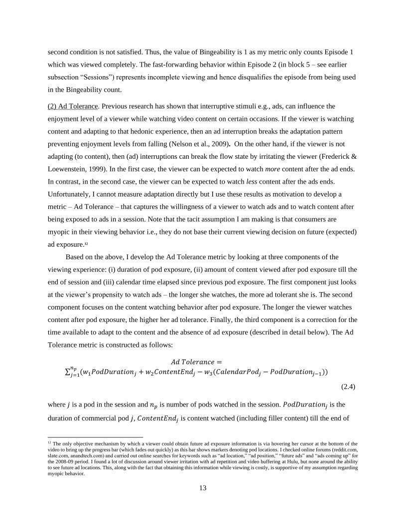
(2) Ad Tolerance. Previous research has shown that interruptive stimuli e.g., ads, can influence the

enjoyment level of a viewer while watching video content on certain occasions. If the viewer is watching

content and adapting to that hedonic experience, then an ad interruption breaks the adaptation pattern

preventing enjoyment levels from falling (Nelson et al., 2009). On the other hand, if the viewer is not

adapting (to content), then (ad) interruptions can break the flow state by irritating the viewer (Frederick &

Loewenstein, 1999). In the first case, the viewer can be expected to watch more content after the ad ends.

In contrast, in the second case, the viewer can be expected to watch less content after the ads ends.

Unfortunately, I cannot measure adaptation directly but I use these results as motivation to develop a

metric – Ad Tolerance – that captures the willingness of a viewer to watch ads and to watch content after

being exposed to ads in a session. Note that the tacit assumption I am making is that consumers are

myopic in their viewing behavior i.e., they do not base their current viewing decision on future (expected)

ad exposure.12

Based on the above, I develop the Ad Tolerance metric by looking at three components of the

viewing experience: (i) duration of pod exposure, (ii) amount of content viewed after pod exposure till the

end of session and (iii) calendar time elapsed since previous pod exposure. The first component just looks

at the viewer’s propensity to watch ads – the longer she watches, the more ad tolerant she is. The second

component focuses on the content watching behavior after pod exposure. The longer the viewer watches

content after pod exposure, the higher her ad tolerance. Finally, the third component is a correction for the

time available to adapt to the content and the absence of ad exposure (described in detail below). The Ad

Tolerance metric is constructed as follows:

𝐴𝑑 𝑇𝑜𝑙𝑒𝑟𝑎𝑛𝑐𝑒 =

∑ (𝑤1𝑃𝑜𝑑𝐷𝑢𝑟𝑎𝑡𝑖𝑜𝑛𝑗 +𝑤2𝐶𝑜𝑛𝑡𝑒𝑛𝑡𝐸𝑛𝑑𝑗 −𝑤3(𝐶𝑎𝑙𝑒𝑛𝑑𝑎𝑟𝑃𝑜𝑑𝑗 − 𝑃𝑜𝑑𝐷𝑢𝑟𝑎𝑡𝑖𝑜𝑛𝑗−1))𝑛𝑝𝑗=1

(2.4)

where 𝑗 is a pod in the session and 𝑛𝑝 is number of pods watched in the session. 𝑃𝑜𝑑𝐷𝑢𝑟𝑎𝑡𝑖𝑜𝑛𝑗 is the

duration of commercial pod 𝑗, 𝐶𝑜𝑛𝑡𝑒𝑛𝑡𝐸𝑛𝑑𝑗 is content watched (including filler content) till the end of

12 The only objective mechanism by which a viewer could obtain future ad exposure information is via hovering her cursor at the bottom of the video to bring up the progress bar (which fades out quickly) as this bar shows markers denoting pod locations. I checked online forums (reddit.com, slate.com, anandtech.com) and carried out online searches for keywords such as “ad location,” “ad position,” “future ads” and “ads coming up” for the 2008-09 period. I found a lot of discussion around viewer irritation with ad repetition and video buffering at Hulu, but none around the ability to see future ad locations. This, along with the fact that obtaining this information while viewing is costly, is supportive of my assumption regarding myopic behavior.

14

the session after watching commercial pod 𝑗, 𝐶𝑎𝑙𝑒𝑛𝑑𝑎𝑟𝑃𝑜𝑑𝑗 is calendar time elapsed from the beginning

of the previous pod in the same session till the beginning of pod 𝑗, 𝑃𝑜𝑑𝐷𝑢𝑟𝑎𝑡𝑖𝑜𝑛𝑗−1 is the duration of

commercial pod 𝑗-1 and 𝑤1, 𝑤2, 𝑤3 are the weights associated with the three components in the equation.

Initially, I set the value of each of the weights to one (and in Appendix A.3, I show that the optimization

outcomes are not sensitive to these weights). Note that though the unit of Ad Tolerance is minutes and its

range is the real number line, it cannot be directly interpreted as a temporal measure. Its magnitude

represents the willingness of the viewer in a session to watch ads and to watch content after being

exposed to ads. A negative value of Ad Tolerance suggests that the viewer stopped watching content

immediately after being exposed to a pod which was preceded (at some point) by a long period of no ad

exposure. I now explain the importance of each component of the Ad Tolerance metric in equation (2.4).

i. 𝑃𝑜𝑑𝐷𝑢𝑟𝑎𝑡𝑖𝑜𝑛𝑗: Duration of a pod

When a viewer is exposed to a commercial pod, each passing second of the pod contributes to the

viewer’s willingness to be exposed to the pod. This is captured by 𝑃𝑜𝑑𝐷𝑢𝑟𝑎𝑡𝑖𝑜𝑛𝑗, the duration of the 𝑗𝑡ℎ

pod that is watched in the session. While a viewer does not have the option to fast-forward, rewind or skip

ads, a viewer can partially watch a pod by exiting the session in the middle of the pod, refreshing the

browser or skipping to the next episode in sequence. Hence, 𝑃𝑜𝑑𝐷𝑢𝑟𝑎𝑡𝑖𝑜𝑛𝑗 captures the willingness of

the viewer to be exposed to the pod.

ii. 𝐶𝑜𝑛𝑡𝑒𝑛𝑡𝐸𝑛𝑑𝑗: Content time watched till end of the session

𝐶𝑜𝑛𝑡𝑒𝑛𝑡𝐸𝑛𝑑𝑗 measures the time spent watching content till the end of the session after being exposed to

pod 𝑗. Longer durations suggest higher tolerance for the previous interruption (with Schweidel and Moe

(2016) finding empirical evidence that content viewership decreases on average as ad exposure increases).

To reduce potential bias in my estimates of 𝐶𝑜𝑛𝑡𝑒𝑛𝑡𝐸𝑛𝑑𝑗, I operationalize the measure of

𝐶𝑜𝑛𝑡𝑒𝑛𝑡𝐸𝑛𝑑𝑗 as the minimum of (a) Content Time in a block and (b) the difference between Session

Time and Ad Time in a block. As mentioned earlier, a block is a period of time from the beginning of a

pod (or beginning of session) till the beginning of the next pod (or end of episode/session). If a viewer

keeps excessively fast-forwarding content, Content Time would increase without a corresponding increase

in Session Time (calendar time). As a result, using Content Time will positively bias the measure of

𝐶𝑜𝑛𝑡𝑒𝑛𝑡𝐸𝑛𝑑𝑗 as the viewer is not actually watching content but is only fast-forwarding content. In such

situations, the metric adds option (b) which is smaller than option (a), thereby eliminating the above bias.

This correction is termed as ‘Caveat 1’ in the rest of the essay.

15

iii. 𝐶𝑎𝑙𝑒𝑛𝑑𝑎𝑟𝑃𝑜𝑑𝑗 − 𝑃𝑜𝑑𝐷𝑢𝑟𝑎𝑡𝑖𝑜𝑛𝑗−1: Inter-pod calendar time

In my setting, when a viewer is not watching ads, she is either watching content, fast-

forwarding/rewinding content or engaged in a break/pause. During this period, the viewer can be expected

to simultaneously adapt to both the content and the absence of ad exposure. The third term captures this

period because it is a measure of the calendar time elapsed since the previous pod exposure. This is the

time during which the level of potentially unfavorable affective intensity resulting from ad exposure can

go down.

𝐶𝑎𝑙𝑒𝑛𝑑𝑎𝑟𝑃𝑜𝑑𝑗 measures the calendar time from the beginning of the previous pod, 𝑗-1, in the same

session till the beginning of pod 𝑗. For the first pod in the session, 𝐶𝑎𝑙𝑒𝑛𝑑𝑎𝑟𝑃𝑜𝑑𝑗 measures the time from

the beginning of the session as there is no previous pod watched in the session. 𝑃𝑜𝑑𝐷𝑢𝑟𝑎𝑡𝑖𝑜𝑛𝑗−1 is the

duration of the 𝑗-1 pod that is watched in the session. The difference between 𝐶𝑎𝑙𝑒𝑛𝑑𝑎𝑟𝑃𝑜𝑑𝑗 and

𝑃𝑜𝑑𝐷𝑢𝑟𝑎𝑡𝑖𝑜𝑛𝑗−1 is the measure of the ad-free time before the beginning of 𝑃𝑜𝑑𝐷𝑢𝑟𝑎𝑡𝑖𝑜𝑛𝑗. This

measure of ad-free time is subtracted from 𝐶𝑜𝑛𝑡𝑒𝑛𝑡𝐸𝑛𝑑𝑗 in equation (2.4) to get the net effect of the

affective influence of an interruption on the viewer.

Next, I apply the Ad Tolerance metric to the illustrative example discussed earlier in Table 2.2, and

this computation is shown in Table 2.4. More illustrative examples are shown in Appendix A.1. In this

example, I begin by adding the duration of the first pod which is 0.66 minutes to the amount of content

viewed in the remainder of the session (after the end of the pod), which is [ 10 + 10 + 2 + 2 + 17 + 0 =

41 ] minutes. It is important to note the use of ‘Caveat 1’ in block 5 (see Table 2.2) where there is

evidence of fast-forwarding behavior. 𝐶𝑜𝑛𝑡𝑒𝑛𝑡𝐸𝑛𝑑𝑗 is chosen as 𝑆𝑒𝑠𝑠𝑖𝑜𝑛 𝑇𝑖𝑚𝑒 – 𝐴𝑑 𝑇𝑖𝑚𝑒, [

17.66 – 0.66 = 17 ] minutes, because it is less than 𝐶𝑜𝑛𝑡𝑒𝑛𝑡 𝑇𝑖𝑚𝑒 of 21 minutes. Then I subtract the

difference between the time elapsed since the beginning of the session and duration of the previous pod,

which are both 0 minutes in this case. Thus, the total value of the metric for the first pod is 41.66

minutes. Then, I repeat this process for the second pod. The second pod is 0.50 minutes long, to which I

add the amount of content viewed in the remainder of the session which is [10 + 2 + 2 + 17 + 0 = 31]

minutes. Then I subtract the difference between the time elapsed since the beginning of the previous pod

and duration of the previous pod, which is [10.66 – 0.66 = 10] minutes. Thus, the total value of the

metric for the second pod is 21.5 minutes. The same process is repeated for each of the remaining pods.

On summing up the values corresponding to each pod, I get a total Ad Tolerance value of 67.98 minutes.

16

2.3.2 Data Summary via Metrics

For my sample comprising 110,500 sessions,13 Bingeability ranges from 0 to 57 (median is 1 episode)

while Ad Tolerance ranges from −412.17 to 63,449.10 minutes (median is 23.62 minutes) (see Table

2.5). The frequency distribution of Bingeability and Ad Tolerance in shown in Figure 2.3a and 2.3b. The

most common value of Bingeability is one (complete episode) in a session. Thus, most of the sessions are

not spent watching multiple episodes of the same TV show in my data. The distribution of Ad Tolerance

is very right skewed. There is large peak between 0 and 3 minutes for more than 10,500 sessions. More

than 16% of these sessions are those in which viewers end the session in less than a minute of calendar

time. This suggests that there are many occasions when viewers are averse to seeing ads at the beginning

of a session (pre-roll ads).

The relationship between the two metrics is shown in the jitter plots (around the values of

Bingeability) in Figure 2.3c, where the darker areas indicate regions of high overlap. The correlation

between Ad Tolerance and Bingeability is 0.68 over the full range of the two metrics and is 0.60 over the

2.5th to 97.5th percentile range of the two metrics. This provides some model free evidence that both

metrics are complementary in terms of describing viewer behavior.

2.3.4 Metric Validity

Given that the two proposed metrics are deterministic transforms of the raw data, it is important for me to

establish that they are valid and informative in terms of capturing viewer behavior. In the interest of

brevity, I provide a summary of this analysis – full details are reported in Appendix A.4. I first compare

the Bingeability metric to the commonly used industry metric for binge-watching – the raw count of

episodes, typically unique, watched of the same TV show in one session (West, 2013). Unlike the raw

count of episodes, the Bingeability metric considers whether viewers watch each episode completely by

explicitly accounting for skipping or excessive fast-forwarding behavior. This allows for a much more

precise measure of content consumption. The correlation between Bingeability and raw episode count is

0.85 over the full range and 0.70 over the 2.5th to 97.5th percentile range of Bingeability. The lack of

perfect (or close to perfect) correlation suggests that the Bingeability metric captures information distinct

from that in episode count. There are no comparable metrics to Ad Tolerance in practice or academic

research to the best of my knowledge. In order to test the validity of my metric, I check for evidence of

correlation between the metric and other “intuitive” measures of ad tolerance: number of pods shown,

minutes of ad exposure and minutes of content viewed. The correlations are 0.78, 0.77 and 0.78

respectively, pointing to the fact that the metric captures distinctive information. Moreover, as shown in

13 The Ad Tolerance metric is undefined for the 12,117 sessions where there is no ad exposure and so I exclude them.

17

Appendix A.4, I find that this metric captures differences in behavioral consumption patterns better than

intuitive measures. Overall, for both metrics, the distinctive information captured suggests face validity

(cf. Ailawadi et al. (2003)).

2.4 Stage II

In this stage, I use the available information to predict the viewing behavior (summarized by the two

metrics) of a new session, for either a current or a new viewer watching an existing or new TV show. In

the first step, I lay out the information that is used (Feature Generation) and in the second, I lay out the

predictive methods (Model).

2.4.1 Feature Generation

The high granularity of my data allows me to include a rich set of features to help predict viewer behavior

during a session. I use current and past viewing activity on Hulu to choose these features. In order to

include both weekdays and weekends, I use a seven-day moving window to capture past viewing activity.

The features I use fall into four types.

(1). Current Behavior

These features (listed in Table 2.6a) characterize the current behavior of viewers in the session. They

include fixed effects for viewer (6157), show (558), genre14 (18), month (5), week (5), day (2) and time of

day (5) as well as continuous variables for episode length of the first episode viewed (1), number of

episodes of the TV show ahead in sequence (1) and number of unwatched episodes of the TV show

during my sample period (1). These features do not depend on a viewer’s historical activity. As my model

(in subsection “Model”) can handle multicollinearity among the features to make predictions, I include

fixed effects for both show and genre, and then later determine the relative importance of the predictors in

the section “Results”. Since an individual viewer’s content consumption and ad response may vary as a

function of where a current episode of a TV show is in the show’s entire chronology, I include two related

measures to capture this. First, I measure the number of episodes of the TV show ahead in sequence

(𝑁1) after the first episode viewed in the current session. Second, I measure the number of potentially

unwatched episodes of the TV show (𝑁2) by subtracting the number of episodes viewed till date (during

my sample period) from the total episodes available in my dataset.15 In total, I have 6,753 features in this

type.

14 If a TV show is labelled with multiple genres (0.08% of the sessions), I use the first genre label assigned to it in the data. 15 Though 𝑁1 and 𝑁2 are correlated (rho=0.73), I use both to capture behavior in the most comprehensive manner, given that I am inferring the inventory at Hulu at any given time (as I do not have access to the actual episode supply). In spite of these measures, I could still miss episodes if they are not viewed by anyone in my dataset at the time of the session and/or if they were available only for a limited time.

18

(2) Ad Targeting Rules

The four ad targeting rules (discussed in the earlier subsection “Ad Delivery”) can be summarized using

features as follows:

• Spacing Rule (SR) is the “mean time between pods in an episode” averaged across all

episodes viewed in a session.16

• Length Rule (LR) is the “mean pod length in an episode” averaged across all episodes viewed in

a session.

• Diversity Rule (DR) is the mean of ad diversity per episode across all episodes viewed in a

session.

• Clumpiness Rule (CR) is the mean of clumpiness in pod locations per episode across all episodes

viewed in a session.17

The absolute value of the correlation between every pair of the rules ranges from 0.16 to 0.51 which

shows that the rules are not too strongly correlated, thus providing evidence that each one is capturing a

distinct underlying decision rule.

(3) Past Behavior: Watching TV Shows Only

I construct 9 functions to systematically generate 68 features (listed in Table 2.6b) that characterize many

aspects of viewers’ TV-viewing behavior at the level of show, day of week, and time of day (cf.

Yoganarasimhan (2019)). The features are computed using all TV-show-viewing activity for a user during

the one-week window before their current session. For instance, if a viewer decides to watch some TV

show on Sunday at 5 pm, I consider all of her sessions watching TV shows that began in the 168 (7*24)

hours before Sunday at 5 pm. This moving window of one week is chosen so that I have adequate

information of a viewer’s recent historical viewing activity that includes both weekdays and weekends. I

generate functions that vary with day and time of day to explore whether experiences that occur at

specific times in the past are significant predictors of Bingeability and Ad Tolerance.

I explain one function in detail and show how its features are generated. The features for the other

functions are generated similarly.

a) Bingeability Sum (Show, Day, Time of Day): This function calculates the past one-week sum of

Bingeability of the viewer for the Show she is about to watch over that Day at that Time of Day.

I consider Day as a Weekend or a Weekday and Time of Day as one of the five: Early Morning:

16 I do not consider time from the last pod shown in an episode till the end of an episode because a viewer could have stopped watching an episode at any time and not have waited till the end of the episode.

17 For 2.5% of sessions where a viewer switches between the same episodes, (e.g., watches episode 1 - episode 2 - episode 1 - episode 2), an episode's ad targeting rule is found by averaging the rule value over each individual occurrence of the episode.

19

7–10am, Day Time: 10am–5pm, Early Fringe: 5pm – 8pm; Prime Time: 8pm – 11pm, Late

Fringe: 11pm – 7am (Schweidel & Moe, 2016). For example, if a viewer decides to start

watching the TV show House on a Weekend during Day Time, then the function will calculate the

sum of Bingeability over all the sessions in the past week when the viewer viewed House on the

Weekend during Day Time. More features can be generated by the function when the three

variables – Show, Day or Time of Day, are dropped in turn from the function using a 23 design.

Thus, a total of 8 features corresponding to Bingeability Sum (BS) can be generated for each

session in my sample, and these are shown in Table 2.6c.

I note that for the first session of each viewer in the panel data, the value of features based on past

behavior is 0 because past observations are censored. This is true for 5.6% of the sessions in my sample

corresponding to 6,157 viewers. I do not drop these as they help me replicate situations when a new

viewer joins the platform.

(4) Past Behavior: Watching TV Shows or Movies

Even though the target behavior that I study is viewing of TV show content and ads, I still consider past

movie-viewing behavior. This allows me to measure how ad exposure in the past week while watching a

movie or a TV show influences the decision to see a TV show in the current session. I construct 11

distinct functions that generate 136 features (listed in Table 2.6d) which consider historical one-week

sessions in which either TV shows or movies were seen. I replace ‘Show’ with ‘Title’ in the name of

these functions to indicate that when ‘Title’ is absent, the viewer could have watched either a TV show or

a movie in the past week.

I explain two functions in detail and show how their features are generated. The features for the

other functions are generated similarly.

a) Pod Count (Pod Length, Title, Day, Time of Day): This function calculates the past one-week

sum of the number of pods of length equal to some Pod Length, shown to the viewer for that

Title over that Day at that Time of day. Based on the histogram of Pod Length shown earlier in

Figure 2.3a, I divide Pod Length into 3 categories: 1 (1 – 26 sec), 2 (26 – 52 sec) and 3 (>52 sec).

I use the same breakdown for the categories as that used for Ad Length in the subsection “Ad

Delivery” because more than 99% of the pods in my data have only 1 ad. This function generates

a total of 32 features from this 4x2x2x2 design: Pod Length (4: 1, 2, 3, __ ) x Title (2: Title, __ ) x

Day (2: Day, __ ) x Time of Day (2: Time of day, __ ), where ‘__’ corresponds to ‘any value’ as

shown in Table 2.6c.

b) Ad Diversity (Title, Day, Time of Day): This function finds the past one-week average of the

percentage of diverse ads shown in each session (in which there was ad exposure) for the viewer

20

watching that Title over that Day at that Time of day. As I do not have a unique Ad ID for each

ad in my dataset, I use a combination of Ad Industry (16 categories such as CPG, Telecom, etc.)

and Ad Length (3 categories) to generate 48 unique ad combinations.

2.4.2 Model

Model Setup. Given the set of chosen features (above), I need to develop a methodology to predict my key

summaries of viewing behavior – Bingeability and Ad Tolerance – for a future session. The total number

of features generated in the previous subsection “Feature Generation” is large (6,961). In order to capture

the effects of this large set of features in the most flexible way, including non-linearities and interactions,

I use machine learning methods (Lemmens & Croux, 2006; Neslin et al., 2006; Rafieian &

Yoganarasimhan, 2019; Yoganarasimhan, 2019). These predictive methods also have the additional

advantage of being scalable, handling many features for many users, and computationally efficient. Since

I want to understand importance of different features and interpret those features’ relationships with the

outcomes, I use tree-based machine learning models. I express my model as follows:

𝑌𝑡 = 𝑓1(𝑋1𝑡, 𝑋2𝑡, 𝑋3𝑡 , 𝑋4𝑡 ,𝑊1𝑡,𝑊2𝑡) + 𝑢𝑡 (2.5)

where 𝑌 is the metric of interest (Ad Tolerance or Bingeability),18 the subscript 𝑡 denotes a session and 𝑓1

is a non-linear function of all the features. 𝑋1, 𝑋2, 𝑋3 and 𝑋4, are the Spacing Rule (SR), Length Rule

(LR), Diversity Rule (DR) and Clumpiness Rule (CR), respectively (as detailed earlier); 𝑊1 is the matrix

of features describing current behavior listed in Table 2.6a; 𝑊2 is the matrix of features describing past

behavior listed in Table 2.6c and 2.6d; and 𝑢 is the error, which is assumed to be additively separable.

I assume 𝑊1 and 𝑊2 to be exogenous as they are determined before the session begins, and I

assume there is no autocorrelation between the errors 𝑢𝑡. However, as noted earlier, the data patterns

suggest that the 𝑋 variables, which represent the ad targeting rules, are not set exogenously to the

behavior of interest. In other words, they could be endogenous due (primarily) to simultaneity, i.e., 𝑋′s

could be set depending on the value of 𝑌. For example, as Bingeability or Ad Tolerance (𝑌) increases, the

mean spacing between pods (𝑋1) could increase because the streaming provider may only have a limited

inventory of ads to deliver for that show at that time, leading to an average decrease in the frequency of

pod spacing (if no other ads are available to compensate). The trade press has noted that low ad inventory

was a frequent occurrence at Hulu around the time of my data (Sloane, 2019).

If this potential endogeneity is not corrected for, then my predicted outcomes will be biased,

leading to non-optimal ad scheduling recommendations. I correct for this using instrumental variables.

18 In Appendix A.5, I show how my approach can be modified to model the two Y’s jointly. Given that there isn’t a meaningful difference in the final recommendations, the additional benefit of doing so seems to be less than the additional methodological complexity required.

21

These instruments should affect 𝑌 only through their effect on 𝑋𝑖 , 𝑖 = {1,2,3,4}, i.e., be uncorrelated with

unobservables 𝑢. I leverage the institutional detail that Hulu has been known to match sponsors with

specific TV shows (Dubner, 2009). Therefore, ad schedules in an episode of a TV show for a focal viewer

are likely to be correlated with ad schedules in the same episode for another viewer (while not depending

on the focal viewer’s viewing behavior). I construct episode-level instruments 𝑍𝑖, for each 𝑋𝑖, 𝑖 =

{1,2,3,4}, in the same spirit as the instruments in Nevo (2000). I define 𝑍𝑖𝑡 to be the mean of 𝑣𝑖 for all

other viewer-episode pairs (involving any of the episodes viewed in session 𝑡) that began before the start

of session 𝑡, where 𝑣1 = time between pods, 𝑣2 = pod length, 𝑣3 = ad diversity and 𝑣4 = clumpiness.

Note that 𝑍𝑖𝑡 can affect 𝑌𝑡 only through its effect on 𝑋𝑖𝑡, because the focal viewer is unaware about the

value of 𝑍𝑖𝑡 that was experienced by other viewers. This is a reasonable assumption for two reasons.

First, my sample is a random draw from all Hulu viewers, lowering the chance that any two viewers

would know each other at all. Second, at the time of my data, there is no discussion around ad delivery on

Hulu’s Facebook page, which was the brand’s major online social media site at the time. In terms of the

empirical relationship between 𝑋𝑖 and 𝑍𝑖 , I find that the raw correlation between them for 𝑖 = {1,2,3,4} is

reasonable at 0.35, 0.25, 0.27 and 0.33.19

Estimation Approach. The first stage of the estimation process can be expressed using a model of 𝑋𝑖 as a

function of 𝑍𝑖 (𝑖 = {1,2,3,4}), 𝑊1 and 𝑊2 as shown below:

𝑋𝑖𝑡 = 𝑔𝑖(𝑍1𝑡 , 𝑍2𝑡 , 𝑍3𝑡 , 𝑍4𝑡 ,𝑊1𝑡,𝑊2𝑡) + 𝑒𝑖𝑡 (2.6)

where, 𝑔𝑖 is a non-linear function and 𝑒𝑖 is the error term assumed to be additively separable with an

expected value of 0. The estimates of the outcome variables from the above first-stage model can then be

plugged as inputs to the second-stage model. The second stage of the estimation process can be expressed

using a model of 𝑌 on �̂�𝑖𝑡 (estimates of 𝑋𝑖 from the first-stage) as well as on 𝑊1 and 𝑊2:

𝑌𝑡 = 𝑓2(�̂�1𝑡, �̂�2𝑡, �̂�3𝑡 , �̂�4𝑡,𝑊1𝑡 ,𝑊2𝑡) + 𝑢𝑡 (2.7)

19 The correlation between the instrument and the endogenous variables does not increase if the instruments are calculated over respective geographical states or regions of the focal viewer’s permanent address, which indicates that the ad targeting rules are unlikely to vary by geographical location of the viewer (assuming the viewer primarily watches content in the state/region of her permanent address which is the only address that is recorded in the data). I also find that show-level instruments (in comparison to episode-level instruments) have a lower correlation with the endogenous variables which suggests that ad characteristics are determined by the platform at the granular episode level and not the show level. Hence, I use episode-level instruments and not show-level instruments.

22

where 𝑓2 is a non-linear function, 𝑢 is the error term of the second-stage ,which is assumed to be

additively separable with an expected value of 0, and 𝑌𝑡 represents the values of Bingeability and Ad

Tolerance.20

The use of instrumental variables along with machine learning methods is nascent, with no prior

research in marketing using it, to the best of my knowledge. The machine learning literature has just

begun to explore the use of instrumental variable approaches to infer causality. Two notable examples are

Hartford et al. (2017) , which uses a deep learning framework with instrumental variables to make

counterfactual predictions of the outcome, and Athey et al. (2019), which uses random forests with

instrumental variables to find asymptotic marginal effects.

To decide which tree-based method to use,21 I compare the performance of different methods

using simulated data, so that I know the ground truth which is unlike the case with my observed dataset

where I do not know the true explanatory power of the features (cf. Hartford et al. (2017)). I consider two

popular tree-based machine learning methods known for their ability to get close to the ground truth –

Extreme Gradient Boosting (XGBoost) and Random Forests (Breiman, 2001; Chen & Guestrin, 2016).

Their performance is also compared with the traditional linear two-stage least squares (2SLS) approach.

My goal is to choose the better performing method for both the first and second stage of the model.

Appendix A.6 describes the two methods, the simulation, and the results, which show XGBoost gets

closest to the ground truth. My findings are consistent with past literature and the results of prediction

competitions that have found gradient boosting methods, and especially XGBoost, to predict better on

average than Random Forests (Olson et al., 2017; Oughali et al., 2019; Synced, 2017). Thus, my results

are all based on the XGBoost method (implemented on a 4 core CPU with two threads per core at 3.6

GHz) that takes about 2 minutes to run.

2.5 Results

2.5.1 Model Estimation

To estimate the model on the dataset, containing a total of 5,760 viewers, 508 unique shows, and 105,610

sessions (see Table 2.7), I construct a training dataset for calibration and two separate holdout datasets for

estimation. I estimate my model on both future observations of the same set of viewers (Holdout 1) and

observations of a completely new group of viewers (Holdout 2). First, I randomly hold out 500 viewers

and select the remaining 5,260 viewers for training. Then, among these selected viewers, I select

approximately 80% of their initial sessions to form the training sample (74,996 sessions), and 20% of

20 In order to implement the instrumental variables approach, I can only use observations (sessions) for which I have complete information about

𝑍𝑖 , 𝑖 = {1,2,3,4}. I remove 4,536 sessions where no other viewer had viewed those episodes before. Next, I drop 354 viewers who visited the

platform exactly once (as their single sessions cannot be randomly assigned to both the training and holdout data).

21 I also explored other linear models such as LASSO, Ridge Regression and Elastic Net but found that non-linear models fit the data better.

23

their future sessions (21,497 sessions) to form the first holdout sample (Holdout 1). The remaining 500

viewers, with their 9,117 sessions form the second holdout sample (Holdout 2). As one of my objectives

is to allow the streaming platform to build ad schedules for new TV shows that have not yet been viewed

but could be viewed by current viewers or new viewers, I estimate the model on this task too. I allow both

holdout samples to include sessions with 13 (Holdout 1) and 16 (Holdout 2) new TV shows not in the

training data.

Next, I estimate the first-stage model (6) using the training sample and get the estimates �̂�𝑖, 𝑖 =

{1,2,3,4} for both the training and holdout samples. The estimates �̂�𝑖 are then plugged into the second

stage of the model (2.7). I estimate the second-stage model using the training sample and obtain

predictions for the outcomes in the holdout samples. The parameters of the XGBoost model are selected

using 5-fold cross-validation repeated 10 times (Appendix A.7 provides details on the cross-validation

process and parameter tuning). The estimates of the outcome variables will be used as inputs to the ad

scheduling process (detailed in section “Stage III”).

A frequent critique of machine learning methods is that they operate as a “black-box” and yield

results that are not interpretable. I try to address this via the use of two descriptive methods – “feature

importance” and “partial dependence” below. The former can be seen as analogous to the “average

effect” of a covariate (coefficient times mean covariate) in a traditional regression setting while the latter

can be seen as analogous to the “marginal effect” of a covariate (coefficient).

2.5.2 Feature Importance

As the name denotes, this method allows me to identify the features in equation (2.7) that are most

predictive of the outcomes. A commonly used metric to do this is “Variance Reduction” (Hastie et al.,

2009). This is the “gain” achieved when the tree is split on a feature, defined as the maximum reduction

in RMSE (for continuous outcomes, like Ad Tolerance) or Negative Log Likelihood (for discrete

outcomes, like Bingeability). I identify the features that are most frequently split during model training.

Then I compute the gain of a set of multiple related features by summing up the gain for each individual

feature in that set. The percentage gain for each set of features used to split the tree is reported in Tables

2.8a and 2.8b for the top 10 sets of predictive features for Bingeability and Ad Tolerance respectively.

The most important predictors of Bingeability are past predictors of ‘Bingeability Sum’, and

‘Number of episodes ahead in sequence, 𝑁1’ and viewer fixed effects. The most important predictors of

Ad Tolerance are viewer fixed effects, past predictors of ‘Ad Tolerance Sum’ and the past predictors of

‘Pod End’. The fact that individual fixed effects and the sums of past outcomes are important in

predicting the outcomes for a new session is not itself surprising, but this process quantifies their relative

importance and identifies the other important features. The total gain contribution of the four estimated ad

24

targeting rules, 𝑆�̂�, 𝐿�̂�, 𝐷�̂� & 𝐶�̂�, is 9.0% for Bingeability and 8.2% for Ad Tolerance. This indicates that

the four ad targeting rules have an important role to play in predicting the value of the metrics. The

clumpiness of ads (𝐶�̂�) is the most important advertising pattern for predicting Bingeability (with a 4.8%

gain) while the frequency of pod delivery (𝑆�̂�) is the most important advertising pattern for predicting Ad

Tolerance (with a 4.3% gain) (Table 2.8c).

2.5.3 Partial Dependence

I use partial dependence plots (J. Friedman, 2001) to examine the (partial) relationship between the

features and the outcomes, and to the best of my knowledge I am introducing this practice to marketing.

Let 𝑋 = {𝑋1, … , 𝑋𝑑} be the set of all features in the training sample, and 𝑓(𝑋) be the corresponding

prediction function. If 𝑋 can be partitioned into a set of features of interest 𝑋𝑠 and its complement set 𝑋𝑐,

then the partial dependence of the outcome on 𝑋𝑆 is defined as follows:

𝑓𝑠(𝑋𝑆) = 𝐸𝑋𝑐[𝑓(𝑋𝑠, 𝑋𝑐)] = ∫𝑓(𝑋𝑠, 𝑋𝑐)𝑝𝑐(𝑋𝑐)𝑑𝑋𝑐

where, 𝑝𝑐(𝑋𝑐) is the marginal probability density function of 𝑋𝑐. The above equation can be estimated

from a set of training data by averaging out the effects of all the other features 𝑋𝑐 in the model, while

taking into account any correlations among features in 𝑋𝑠 (J. Friedman, 2001; Greenwell, 2017).

Empirically, for a single feature of interest, consider an observation’s value of that feature, and create an

otherwise identical copy of the dataset except substitute that value in for all other observations’ values of

that feature. For the newly edited data, obtain the model’s predictions for each observation and average

the predictions across all observations. Then repeat this for each observation of that feature, plotting

feature values versus average prediction values. This can be better understood as a two-step process:

i. For 𝑖 = {1,… , 𝑛}, where 𝑛 is the number of observations in the training data,

a) Replace each value in 𝑋𝑆 (n-dimensional vector) with 𝑋𝑆𝑖 (constant)

b) Compute predicted values of the 𝑛 outcome variables

c) Find average of the 𝑛 predicted values = 𝑓�̅�(𝑋𝑆𝑖)

ii. Plot {𝑋𝑆𝑖 , 𝑓�̅�(𝑋𝑆𝑖)} for 𝑖 = {1,… , 𝑛} to get the partial dependence plot.

To ease the computational burden, I compute the partial dependence over the deciles of the feature

in addition to its 2.5th and 97.5th percentile. Figure 2.4a shows the relationship between Bingeability and

its most important feature, Bingeability Sum (same Show, any Day, any Time of day). This feature

represents the sum of Bingeability across all sessions shown to the viewer in the past week for the same

25

Show (as the current session) viewed on any Day at any Time of day. The figure shows that an increase in

Bingeability for a show from 0 episodes to 15 episodes over the past week predicts an average increase in

Bingeability for the same show in the current session by 0.6 episodes. The relationship between Ad

Tolerance and its most important feature (other than viewer fixed effects), Ad Tolerance Sum (same Title,

any Day, any Time of day), is shown in Figure 2.4b. This feature calculates the sum of Ad Tolerance

across all sessions shown to the viewer in the past week for the same Title (as the current session) viewed

on any Day at any Time of day. The figure shows that an increase in Ad Tolerance for a title from −16

minutes to 3,513 minutes over the past week predicts an average increase in Ad Tolerance for the same

title in the current session by 710 minutes. Both relationships (in Figures 2.4a and 2.4b) provide evidence

of state dependence between the past and current sessions of a viewer for the same TV show.

As my goal is to make ad scheduling recommendations, I need to understand the relationships

between the ad targeting rules and my two outcome variables. The partial relationships between the ad

targeting rules that are most predictive, clumpiness ( 𝐶�̂� ) and spacing ( 𝑆�̂� ), and the predicted values of

Bingeability and Ad Tolerance respectively, are shown in Figures 2.4c and 2.4d. Lower clumpiness

values, i.e., more equally spaced pods, predict higher Bingeability (Figure 2.4c). Moreover, the extent of

the influence of 𝐶�̂� (over its 2.5th to 97.5th percentile range) on Bingeability is ± 0.44 episodes. The

extent of the influence of 𝑆�̂� (over its 2.5th to 97.5th percentile range) on Ad Tolerance is ± 18.95 minutes

(Figure 2.4d), with most of the change occurring from the 90th percentile (7.7 minutes) to 97.5th percentile

(8.6 minutes) of spacing. This suggests that, on average, spacings longer than 7.7 minutes can overly

adapt viewers to the content and/or absence of ads and increase their aversion to ads.

It is also possible that the ad targeting rules may interact, so I examine the partial dependence of

two predictors jointly. I consider my first pair of predictors of interest to be 𝑋𝑠1 = {�̂�1, �̂�4} = {𝑆�̂�, 𝐶�̂�},

the predicted ad targeting rules that are most important in predicting Bingeability and then the second pair

of predictors 𝑋𝑠2 = {�̂�1, �̂�2, } = {𝑆�̂�, 𝐿�̂�}, since these two rules are most important in predicting Ad

Tolerance. The partial dependences of the estimated values of Bingeability and Ad Tolerance on each pair

of their important predictors are shown in Figure 2.4e and 2.4f. Figure 2.4e shows that the magnitude of

the influence of the top two ad targeting rules (over their 2.5th to 97.5th percentile range) on Bingeability is

± 0.24 episodes. Furthermore, Figure 2.4e shows that higher values of 𝑆�̂� and lower values of 𝐶�̂� predict

higher Bingeability. Similarly, Figure 2.4f shows that the magnitude of the influence of the top two ad

targeting rules (over their 2.5th to 97.5th percentile range) on Ad Tolerance is ± 15.94 minutes, which is

less than the size of the partial dependence on 𝑆�̂� alone, ± 18.95 minutes, found in Figure 2.4d.

Furthermore, Figure 2.4d also shows that lower values of 𝑆�̂� and higher values of 𝐿�̂� predict higher Ad

Tolerance.

26

Finally, I look at the effect of the pairwise interactions (six) across all the four estimated ad

targeting rules 𝑋𝑠3 = {�̂�1, �̂�2, �̂�3, �̂�4} = {𝑆�̂�, 𝐿�̂�, 𝐷�̂�, 𝐶�̂�}. The partial dependences of the estimated

values of Bingeability and Ad Tolerance on 𝑋𝑠3 are calculated over the quintiles of each variable in

addition to their 2.5th and 97.5th percentile to ease computational burden. The extent of the influence of

the four ad targeting rules (over their 2.5th to 97.5th percentile range) on Bingeability is ± 0.25 episodes,

which is about the same as ± 0.24 episodes found in Figure 2.4e. Thus, there is almost no additional

impact on Bingeability. Similarly, the extent of the influence of the four ad targeting rules (over their 2.5th

to 97.5th percentile range) on Ad Tolerance is ± 33.08 minutes, which is more than the extent of ± 15.94

minutes found in Figure 2.4f.

From Table 2.7, the median value of Bingeability in the data is 1 episode and that of Ad Tolerance

is 23.69 minutes. The partial dependence analysis is useful in that it tells me the impact of different

variables (or sets of variables) on the outcome variables. For example, based on the above, I know that the

Ad Targeting rules, in combination can effect a maximum change of 25% (0.25/1.00) on median

Bingeability and a maximum change of 140% (33.08/23.69) on median Ad Tolerance. Overall, these

analyses show that the ad targeting rules, individually and together, have a material impact on viewer

behavior as captured via the two outcomes.

2.6 Stage III

With summaries of behavior predicted and the importance of the features that predict those summaries

understood, in the third stage I use the predicted values of the behavioral summary metrics to make ad

scheduling recommendations. I do this in two steps. First, I provide a guide to the streaming provider on

how to use these predictions with a decision tree, and then I use an optimization procedure to recommend

a better ad schedule in any given session. In order to illustrate the properties of my generated ad schedule

for each session in the holdout samples, I contrast it with the current ad schedule (observed in the data)

and an alternative ad schedule based on a naïve heuristic.

2.6.1 Ad Decision Tree

I propose an “Ad Decision Tree” (Figure 2.5) to identify the types of sessions where ads may enhance –

or at least not detract from – content consumption. The Ad Decision Tree takes in the predictions of

Bingeability and Ad Tolerance obtained from the model and recommends action. The first decision split

in the Ad Decision Tree is to check whether the predicted value of Bingeability is greater than a

threshold, 𝑇. If the predicted value of Bingeability for the session is less than the threshold, then the

streaming platform is advised to not show any ads in the session. This is because there is not much

incentive for a free ad-supported only streaming platform to show ads in a session if the ads are predicted

to prevent the viewer from completing a desired number of episodes (represented by the chosen threshold

27

value for Bingeability). By ensuring that a viewer is predicted to watch at least beyond that threshold, the

streaming platform will be able to provide a minimum level of engagement with the content on its

platform. I examine the impact of increasing the threshold in the subsection “Decision Support System,”

but for now, I start by choosing the lowest Bingeability threshold of 0 episodes i.e., show ads for all

sessions.

If the predicted value of Bingeability is greater than or equal to the threshold, I move to another part

of the tree and check the sign of the predicted value of Ad Tolerance. Negative values of Ad Tolerance

capture occasions where viewers stopped watching content after being exposed to a pod, which itself was

preceded (at some point) by a longer period of no ad exposure. On the other hand, a positive value of Ad

Tolerance indicates occasions where ads were shown more frequently to a viewer and the viewer

continued to watch content.

If the predicted value of Ad Tolerance is > 0, then I solve a novel optimization procedure discussed

in subsection “Optimization”. If the predicted value of Ad Tolerance is ≤ 0, then it is unclear how

tolerant a viewer is towards seeing a pod of ads, so my proposed decision tree recommends testing and

then adapting to what is learned. To test whether the viewer can have both Ad Tolerance > 0 and

Bingeability ≥ 1, the streaming platform is advised to show pods within the first half of each episode to

resemble occasions of frequent ad exposure. To ensure an overall minimum ad exposure within the first

half of an episode, it would be best to show pods at an interval of a quarter of the episode length with

“regular interruptions” (discussed further in subsection “Optimization”). Based on the viewer’s response

to the ad exposure in the first half of the episode, if the viewer continues to have Bingeability ≥ 1, then

the viewer’s Ad Tolerance is updated to > 0 and the rest of the optimization procedure can be

implemented.

The recommendations made by the Ad Decision Tree for the observations in the two holdout

samples are summarized in Table 2.9. I find that for most of the sessions in both holdout samples (94% of

observations in Holdout 1 and 97% of observations in Holdout 2 – see Set C, Table 2.9), the

recommendation to the streaming provider is to use the proposed optimization procedure.

2.6.2 Optimization

In this research, I have set the objective of a streaming provider to maximize ad exposure (to earn more ad

revenue) subject to the constraint of not detracting from the consumption experience. I can express the

maximization of the objective function for a given session as follows:

max𝑓(𝑛, 𝑑) = ∑ 𝑑𝑗𝑛𝑗=1 where ∑ 𝑠𝑗

𝑛𝑗=1 + 𝑠′ = �̂�𝑒⏞

expected content watched

(2.8)

28

where, 𝑛 is the number of pods shown in a session, 𝑑𝑗 is the duration (length) of pod 𝑗, 𝑠𝑗 is the spacing

(content time shown) between pod 𝑗-1 (or beginning of session if 𝑗=1) and pod 𝑗, 𝑠′ is the duration of

content time shown after the end of pod 𝑛, �̂� is the estimated Bingeability from the model, and 𝑒 is the

average episode length of all episodes of the TV show watched in that session in my dataset.

My findings in subsection “Partial Dependence” showed that lower values of clumpiness (i.e., more

equal spacings between pods) result in higher values of Bingeability. In addition, past literature has

shown that viewers are less likely to adapt to irregular sources of interruptions, such as dormitory noise or

aircraft noise (Frederick & Loewenstein, 1999). Hence, it is likely that having regularity in interruptions

would assist the adaptation process and increase Bingeability. Unequal spacing 𝑠𝑗 between pods and

unequal duration 𝑑𝑗 for each pod are sources of irregularity. To remove irregularities within a session, I

let the duration of each pod 𝑑𝑗 be equal to 𝑑 and let the duration of each spacing 𝑠𝑗 and 𝑠′ be equal to 𝑠.

Consequently, I rewrite the optimization as follows:

max𝑓(𝑛, 𝑑) = 𝑛𝑑 where 𝑠(𝑛 + 1) = �̂�𝑒 (2.9)

where the product of spacing between pods, 𝑠, and number of pods plus one, 𝑛 + 1, should equal the

product of predicted Bingeability, �̂� , and average episode length, 𝑒. The constraint 𝑠(𝑛 + 1) = �̂�𝑒 allows

only mid-roll ads (i.e., no pre-roll ads or post-roll ads). This is because prior work has found that viewers

are more likely to completely view mid-roll ads, followed by pre-roll ads and finally post-roll ads

(Krishnan & Sitaraman, 2013). Note that the subsection on “Decision Support System” relaxes this

constraint to allow for pre-roll ads.

My objective function is subject to the constraint of not detracting from the content consumption

experience i.e., not exceeding the predicted Ad Tolerance for a session. Using equation (2.4) and a series

of stepwise substitutions shown in Appendix A.8 (Part 1), this constraint can be expressed as follows:

�̂� = 𝑤1𝑛𝑑 + 𝑤2 (𝑛�̂�𝑒 −𝑛(𝑛+1)

2𝑠) − 𝑤3𝑛𝑠 (2.10)

where 𝑤1, 𝑤2, 𝑤3 are the three weights, originally present in equation (2.4), and �̂� is the predicted value of

Ad Tolerance. I also have additional constraints that there must be at least one pod, and the duration of a

pod must be non-zero. Therefore, the constrained optimization problem in equation (2.9) can be expressed

as follows along with all its constraints:

max𝑓(𝑛, 𝑑) = 𝑛𝑑 where 𝑠(𝑛 + 1) = �̂�𝑒

such that �̂� = 𝑤1𝑛𝑑 + 𝑤2 (𝑛�̂�𝑒 −𝑛(𝑛+1)

2𝑠) − 𝑤3𝑛𝑠, 𝑛 ≥ 1, and 𝑑 > 0

29

Since I am setting spacing to be a constant function of expected total episode content viewed, I replace 𝑠

with �̂�𝑒

𝑛+1 in the constraints, and then I can re-express my constrained optimization problem as

max𝑓(𝑠, 𝑑) = 𝑛𝑑 (2.11)

such that �̂� = 𝑤1𝑛𝑑 + 𝑤2 (𝑛�̂�𝑒

2) − 𝑤3 (

𝑛�̂�𝑒

𝑛+1) , 𝑛 ≥ 1, and 𝑑 > 0

By applying the Lagrange function to the optimization problem, I get the following expression:

𝐿(𝑛, 𝑑, 𝜆1, 𝜆2, 𝜆3) = 𝑛𝑑 − 𝜆1(�̂� − 𝑤1𝑛𝑑 − 𝑤2 (𝑛�̂�𝑒

2) + 𝑤3 (

𝑛�̂�𝑒

𝑛 + 1)) + 𝜆2(𝑛 − 1) + 𝜆3𝑑

with the following six constraints: (1) 𝜕𝐿

𝜕𝑛= 0 (2)

𝜕𝐿

𝜕𝑑= 0, (3) 𝜆2(𝑛 − 1) = 0, 𝜆3𝑑 = 0 (4) 𝑛 ≥ 1, 𝑑 > 0

(5) �̂� = 𝑤1𝑛𝑑 + 𝑤2 (𝑛�̂�𝑒

2) − 𝑤3 (

𝑛�̂�𝑒

𝑛+1) (6) 𝜆1, 𝜆2, 𝜆3 ≥ 0

I use the fifth constraint to solve for 𝑛, so I get a quadratic equation in 𝑛:

𝑛2(𝑤12𝑑 + 𝑤2�̂�𝑒) + 𝑛(𝑤12𝑑 − (2𝑤3 −𝑤2)�̂�𝑒 − 2�̂�) − 2�̂� = 0 (2.12)

As 𝑑 > 0, and �̂� > 0 , �̂� ≥ 1 (from the Ad Decision Tree), the above equation has one positive root and

one negative root of 𝑛. Solving the other constraints of the Lagrange Function does not give solutions

within the acceptable parameter space. Next, I set the weights, 𝑤1, 𝑤2, 𝑤3, to 1, as originally done in

subsection “Metric Development,” although these can be set differently, which I consider in Appendix

A.3. The two unknown parameters in equation (2.12) are 𝑑 and 𝑛. I fix 𝑑 at 30 seconds,22 the median pod

duration in my dataset, and then solve equation (2.12) for the optimal �̃�, and use its positive root which

can be expressed as follows:

�̃� =−(1−�̂�𝑒−2�̂�)+√Δ

2(1+�̂�𝑒) , where Δ = (�̂�2𝑒2 + 12�̂��̂�𝑒 − 2�̂�𝑒 + 4�̂�2 + 4�̂� + 1) and √Δ > 0 (2.13)

22 I also run the optimization using a fixed pod duration of 15 seconds instead of 30 seconds as the distribution of pod length (Figure 2a) shows a

second peak at 15 seconds. The recommended spacing using 15 seconds and that using 30 seconds is almost identical (and the difference on average

is less than 6 seconds).

30

Therefore, I have found the recommended number of pods �̃� from the optimization routine, and this

implies that the recommended spacing �̃� = �̂�𝑒

�̃�+1. Hence, my optimization procedure recommends the pod

frequency �̃� for a viewer’s session holding pod duration 𝑑 constant.23,24

In order to understand the effect of the estimates of Bingeability, �̂�, and Ad Tolerance, �̂�, on the

recommended number of pods �̃� and pod spacing, �̃� (which is proportional to 1

�̃� ), I take the partial

derivatives of �̃� in (12) with respect to �̂� and then with respect to �̂�. The expressions of the partial

derivatives are shown in Appendix A.8 (Part 2). The partial derivatives suggest that the streaming

provider should on average increase pod spacing (decrease pod frequency) when a viewer is expected to

have lower Ad Tolerance or higher Bingeability, holding the other constant. Similarly, the streaming

provider should on average decrease pod spacing (increase pod frequency) when a viewer is expected to

have higher Ad Tolerance or lower Bingeability, holding the other constant.

To summarize all of these session-by-session ad spacing recommendations, I consider their full

distribution. The density of the recommended spacing for the two holdout samples helps illustrate the

range of recommendations made by the optimization routine (Figures 2.6a and 2.6b). The median value of

the recommended spacing for Holdout 1 (future sessions of the viewers in the training sample) is 4.33

minutes, and its 2.5th to 97.5th percentile range is from 0.61 to 9.80 minutes. The median value of the

recommended spacing for Holdout 2 (new viewers) is 4.43 minutes, and its 2.5th to 97.5th percentile range

is from 0.71 to 9.43 minutes.25 While this may seem like very frequent ad exposure, it is not very different

from that in the data (below). In addition, Nelson et al. (2009) show ads every 2 minutes in their

experiments and current industry practice is experimenting with comparable or even shorter ad spacing

(Gessenhues, 2018). Note that the optimization procedure takes about 10 seconds.

2.6.3 Recommended Schedule: Comparison with Data

In this section, I compare the recommended spacing �̃� for a session with the average observed spacing �̅�

in the session. The average observed spacing for a session is calculated across each of its observed

spacings, 𝑠𝑗 , which is the content time shown between pod 𝑗-1 (or beginning of session if 𝑗=1) and pod 𝑗.

I do not consider the content viewed from the end of the last pod till the end of the session, 𝑠′, as a viewer

could have ended the session before the end of an episode thus biasing the value of 𝑠′.

23 I express the constraint as a quadratic equation in �̃�, and not �̃�, because the product of the roots in the quadratic equation of �̃� is always negative, giving us one positive and one negative root, and helping us choose the positive root. The product of the roots in the quadratic equation of �̃� is always positive, making it harder to choose the appropriate positive root. 24 I do not directly recommend number of pods, �̃�, because the number of pods to be shown is not under direct control of the streaming provider. The streaming provider can only set the spacing (content time) after which a pod must be shown. The total number of pods that the viewer will end up viewing depends on the endogenous decision of the viewer to stop viewing content. 25 I also examined recommendations by show length and genre. For show episodes < 30 mins, the spacing was 4.44 mins (4.26 mins) for Holdout 1 (Holdout 2), while for show episodes > 30 mins, it was 4.22 mins (4.57 mins). For Comedy shows, it was 4.60 mins (4.49 mins), for Drama 4.40 mins (4.76 mins) and for Science Fiction 4.95 mins (5.11 mins).

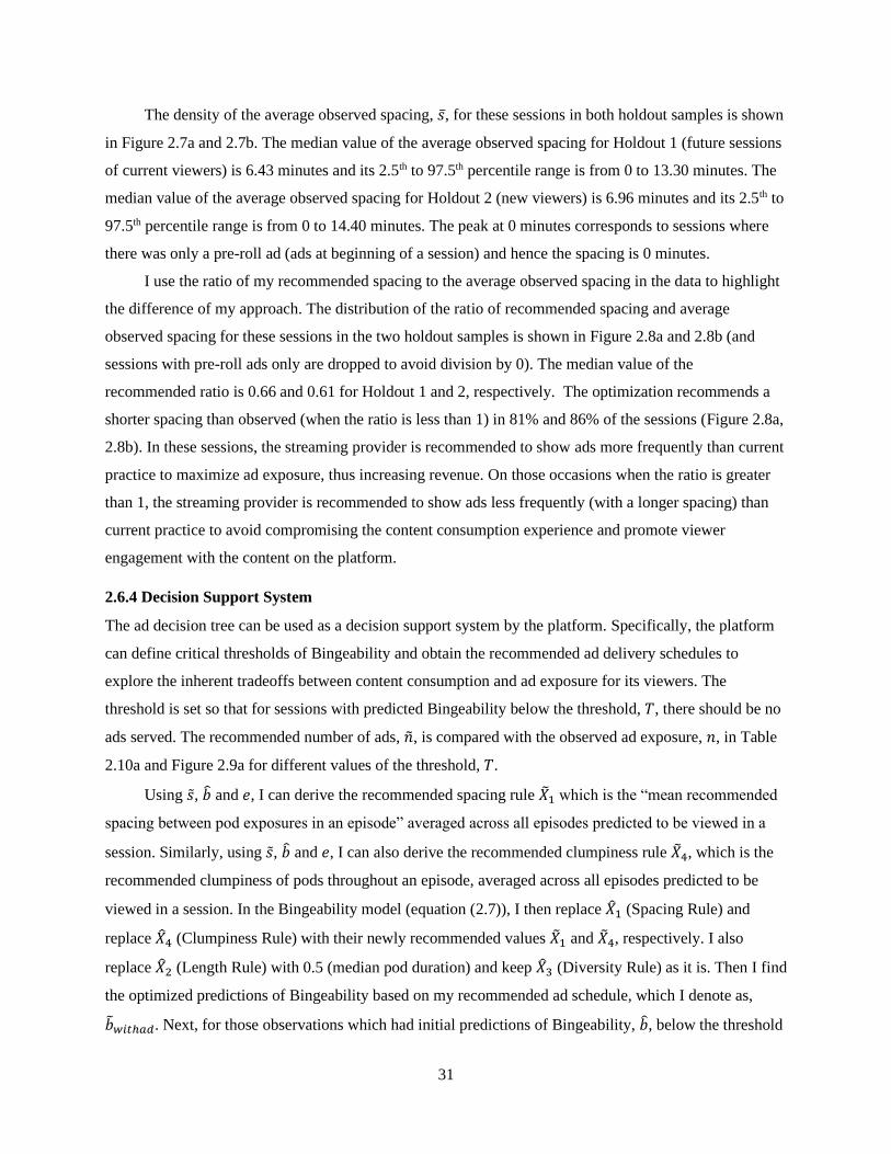
31

The density of the average observed spacing, �̅�, for these sessions in both holdout samples is shown

in Figure 2.7a and 2.7b. The median value of the average observed spacing for Holdout 1 (future sessions

of current viewers) is 6.43 minutes and its 2.5th to 97.5th percentile range is from 0 to 13.30 minutes. The

median value of the average observed spacing for Holdout 2 (new viewers) is 6.96 minutes and its 2.5th to

97.5th percentile range is from 0 to 14.40 minutes. The peak at 0 minutes corresponds to sessions where

there was only a pre-roll ad (ads at beginning of a session) and hence the spacing is 0 minutes.

I use the ratio of my recommended spacing to the average observed spacing in the data to highlight

the difference of my approach. The distribution of the ratio of recommended spacing and average

observed spacing for these sessions in the two holdout samples is shown in Figure 2.8a and 2.8b (and

sessions with pre-roll ads only are dropped to avoid division by 0). The median value of the

recommended ratio is 0.66 and 0.61 for Holdout 1 and 2, respectively. The optimization recommends a

shorter spacing than observed (when the ratio is less than 1) in 81% and 86% of the sessions (Figure 2.8a,

2.8b). In these sessions, the streaming provider is recommended to show ads more frequently than current

practice to maximize ad exposure, thus increasing revenue. On those occasions when the ratio is greater

than 1, the streaming provider is recommended to show ads less frequently (with a longer spacing) than

current practice to avoid compromising the content consumption experience and promote viewer

engagement with the content on the platform.

2.6.4 Decision Support System

The ad decision tree can be used as a decision support system by the platform. Specifically, the platform

can define critical thresholds of Bingeability and obtain the recommended ad delivery schedules to

explore the inherent tradeoffs between content consumption and ad exposure for its viewers. The

threshold is set so that for sessions with predicted Bingeability below the threshold, 𝑇, there should be no

ads served. The recommended number of ads, �̃�, is compared with the observed ad exposure, 𝑛, in Table

2.10a and Figure 2.9a for different values of the threshold, 𝑇.

Using �̃�, �̂� and 𝑒, I can derive the recommended spacing rule �̃�1 which is the “mean recommended

spacing between pod exposures in an episode” averaged across all episodes predicted to be viewed in a

session. Similarly, using �̃�, �̂� and 𝑒, I can also derive the recommended clumpiness rule �̃�4, which is the

recommended clumpiness of pods throughout an episode, averaged across all episodes predicted to be

viewed in a session. In the Bingeability model (equation (2.7)), I then replace �̂�1 (Spacing Rule) and

replace �̂�4 (Clumpiness Rule) with their newly recommended values �̃�1 and �̃�4, respectively. I also

replace �̂�2 (Length Rule) with 0.5 (median pod duration) and keep �̂�3 (Diversity Rule) as it is. Then I find

the optimized predictions of Bingeability based on my recommended ad schedule, which I denote as,

�̃�𝑤𝑖𝑡ℎ𝑎𝑑. Next, for those observations which had initial predictions of Bingeability, �̂�, below the threshold

32

𝑇 (where the platform is advised to not show ads26) I train the Bingeability model without the four ad

targeting rules (�̂�1, �̂�2, �̂�3, �̂�4), and then make revised predictions, �̃�𝑤𝑜𝑎𝑑. I report the net incremental

change in �̃�𝑤𝑖𝑡ℎ𝑎𝑑 + �̃�𝑤𝑜𝑎𝑑 ( = �̃� ) as compared to observed Bingeability 𝑏, and initial predicted

Bingeability �̂�, in Table 2.10b and 2.10c respectively, for different values of the threshold. These

comparisons are also shown in Figure 2.9b and 2.9c for Holdout 1 and Holdout 2 respectively.

The results for Holdout 1 (future sessions of current viewers) and Holdout 2 (new viewers) show

the tradeoff between content consumption (measured through Bingeability) and ad exposure. From Table

2.10a and Figure 2.9a, I see that there is a net increase in ad exposure for thresholds (of predicted

Bingeability) ≤ 0.8 for observations in Holdout 1 and for thresholds ≤ 0.9 for observations in Holdout 2.

A threshold of 0 results in the maximum increase in ad exposure for both Holdout 1 and Holdout 2. From

Table 2.10b & 2.10c and Figure 2.9b & 2.9c, I see that the maximum increase in content consumption for

Holdout 1 is for a threshold of 0, and the maximum increase (or lowest decrease) in content consumption

for Holdout 2 is for a threshold of 1.6.

Overall, for future sessions of current viewers, if the platform uses a threshold of 0 to show ads, the

platform gets more ad exposures and viewers see more content. This results in a 71.2% increase in ad

exposure, as compared to what was observed, and a 5.17% increase in Bingeability as compared to the

initially predicted Bingeability before optimization (or a 5.33% increase in Bingeability as compared to

observed Bingeability).27 On the other hand, for new viewers, there is a tension: the platform is better off

in terms of ads shown if it uses a threshold of 0 to show ads which results in a 79.1% increase in ad

exposure; whereas viewers are better off in terms of content viewed if the platform uses a threshold of 1.6

to show ads which results in a 1.03% increase in Bingeability as compared to the initially predicted

Bingeability (or a decrease of 0.80% in Bingeability as compared to observed Bingeability). This

indicates that for new viewers for whom preferences are unknown, there is no single threshold 𝑇 that can

lead to the best outcome for both the platform and the viewer. The best that can be done in this case is to

compare the optimized Bingeability with initial predicted Bingeability using the same set of features,

giving a 1% increase in content consumption.

It is important to note that for Holdout 1, the best threshold of 0 corresponds to showing ads for

most sessions which results in a net increase in content consumption by 5.2%. This is higher than the net

increase in content consumption of 2.1% for a threshold of 9 that corresponds to not showing ads for most

sessions. This indicates that the decision to show ads for future sessions of current viewers (Holdout 1)

under the optimized ad schedule can make viewers better off as compared to a decision to not show ads.

26 It is important to note that I also do not show ads for those sessions for which �̂� > 𝑇 and �̂̂� < �̃�, i.e., if predicted value of Bingeability is greater than the threshold but less than the recommended spacing, I am unable to show ads. 27 While a 71% increase seems large, it is within the range of the observed data - for Holdout 1, the recommended range of ad exposure is once every 0.01-61.01 minutes (data is 0.00-108.43 minutes) and for Holdout 2 is 0.01-28.94 minutes (data is 0.00-103.38 minutes).

33

I also consider the impact specifically of allowing pre-roll ads. Casual observation suggests that that

it may increase ad exposure but lower content consumption. To test this, I allow for pre-roll ads by

modifying the constraint in equation (2.9) to 𝑠𝑛 = �̂�𝑒, and then I run the optimization routine followed by

the steps outlined in the Decision Support System for a threshold of 0. I find that ad exposure increases

substantially (23%) as compared to ad exposure under my recommendation. However, content

consumption decreases as compared to my recommendation by about 0.7% across both holdout samples.

The decrease in content consumption is driven by the average decrease in mean spacing between pods

that results from allowing pre-rolls ads (in addition to mid-roll ads) for the same level of predicted Ad

Tolerance. Thus, allowing pre-roll ads results in much higher ad exposure but comes at a cost of a very

small reduction in content consumption, a trade-off that a platform may be willing to make.

I also test the performance of a naive heuristic that computes pod spacing as a ratio of the total

content time to the total number of pods for a viewer in a given week (see Appendix A.9 for details). The

best this heuristic can do is to increase content consumption at the expense of decreasing ad exposure

(compared to observed practice) i.e., not delivering a win-win recommendation for the platform and its

viewers.

2.7 Conclusion

This essay adds to the small but growing body of work that investigates the implications of increase in

consumer control vis-à-vis content consumption on streaming media. To the best of my knowledge, this

essay is the first attempt at providing a solution for advertising scheduling in such settings. Specifically, it

provides an approach for streaming providers to explore the tradeoff between content consumption and ad

exposure in order to provide a balanced viewing experience. The recommendations from this approach

are available at the granular level of an individual viewer-session. The approach also uses state-of-the-art

methods such as machine learning, but more importantly allows for causal inference via the use of

instrumental variables and provides increased interpretability of the estimates.

In the first stage of the three-stage approach, I develop two new metrics – Bingeability and Ad

Tolerance – to capture the interplay between content consumption and ad exposure for each session. I

need to do this as there is little standardization around the measurement of content consumption and ad

exposure in streaming media settings. My metrics are motivated by the consumer psychology literature on

flow states and hedonic adaptation as well as observed consumer behavior (in these settings). In the

second stage, I first use feature generation to summarize the current and past viewing environment of

each consumer over a moving one-week window. I then use a novel tree-based instrumental variable

approach to predict the value of the metrics. Using feature importance and partial dependence analyses, I

provide insights into the relative importance of various features in predicting viewer consumption

34

patterns. In the third stage, I pass the predictions from the previous stage through a decision tree and an

optimization routine. This is followed by the construction of a decision support system which allows the

platform to explore the tradeoff between content consumption and ad delivery for both current and new

viewers. The platform can then make choices around its ad schedule for each session given its objective

function. It is important to note that “win-win” ad schedules are possible e.g., for current viewers, I am

able to find schedules that simultaneously allow for higher content consumption (a 5.2% increase in

Bingeability) at higher levels of ad exposure (a 71.2% increase).

My approach could potentially be applied to other ad supported environments, especially where

consumers have control over content consumption e.g., news media consumption. My decision support

system can also be integrated into an online experimentation platform, where recommendations can be

tested in live settings and where the results from experiments can be used to improve the performance of

predictive models.

My work does suffer from some limitations. First, while I believe that my approach is general, it is

calibrated on data from just one streaming provider. Second, my optimization algorithm simplifies ad

scheduling. While it provides conservative results, it can be improved (at the cost of complexity). Third,

even though free ad-supported streaming platforms continue to grow, there are now combinations of

free/paid ad-supported and paid ad-free models available within the same platform. Figuring out ad

scheduling in these settings would necessitate modifications to my approach. Fourth, I cannot link my

optimal ad exposure to final purchase due to lack of data. Finally, given the increasing availability of

different online streaming options on multiple devices, newer patterns of non-linear consumption could

emerge, perhaps requiring the development of other metrics. I hope that future work can address these

limitations.

35

2.8 Tables

Table 2.1: Summary of Sessions

Session (minutes)

N Min 2.5% Median Mean 97.5% Max

122,617 0.02 1.82 42.70 56.06 236.51 1573.03

Table 2.2: Example timeline (in minutes) of viewing behavior in a session

24 min

episode of

Aquarion

0.66 10 0.50 10 0.50 2 2 0.66 21 0.50 0

10.66 11 2.5 2 17.66 1

Table 2.3: Computation of the Bingeability Metric

Table 2.4: Computation of the Ad Tolerance Metric

Example

Expression: ∑ 𝟙 {𝐶𝑜𝑛𝑡𝑒𝑛𝑡 𝐿𝑒𝑛𝑔𝑡ℎ𝑖 − 5 𝑚𝑖𝑛𝑠 ≤ 𝐶𝑜𝑛𝑡𝑒𝑛𝑡 𝑇𝑖𝑚𝑒𝑖 ≤

𝑆𝑒𝑠𝑠𝑖𝑜𝑛 𝑇𝑖𝑚𝑒𝑖 − 𝐴𝑑 𝑇𝑖𝑚𝑒𝑖}

𝑛𝑒𝑖=1

Bingeability

No Skipping:

𝐶𝑜𝑛𝑡𝑒𝑛𝑡 𝐿𝑒𝑛𝑔𝑡ℎ𝑖 − 5 𝑚𝑖𝑛 ≤ 𝐶𝑜𝑛𝑡𝑒𝑛𝑡 𝑇𝑖𝑚𝑒𝑖

No Excessive Fast-forwarding:

𝐶𝑜𝑛𝑡𝑒𝑛𝑡 𝑇𝑖𝑚𝑒𝑖 ≤ 𝑆𝑒𝑠𝑠𝑖𝑜𝑛 𝑇𝑖𝑚𝑒𝑖 −𝐴𝑑 𝑇𝑖𝑚𝑒𝑖

24 min episode of Aquarion Episode 1: 24 − 5 ≤ 22

Episode 2: 24 − 5 ≤ 21

Episode 1: 22 ≤ 24.16 − 1.66

Episode 2: 21 ≰ 20.66 − 1.16

1

Example Expression: ∑ (𝑃𝑜𝑑𝐷𝑢𝑟𝑎𝑡𝑖𝑜𝑛𝑗 + 𝐶𝑜𝑛𝐸𝑛𝑑𝑗 − (𝐶𝑎𝑙𝑃𝑜𝑑𝑗 − 𝑃𝑜𝑑𝐷𝑢𝑟𝑎𝑡𝑖𝑜𝑛𝑗−1))𝑛𝑝𝑗=1

Ad Tolerance

(minutes)

24 min episode of

Aquarion

• Pod 1: 0.66 + (10 + 10 + 2 + 2 + 17 + 0) − (0 − 0) = 41.66

• Pod 2: 0.50 + (10 + 2 + 2 + 17 + 0) − (10.66 − 0.66) = 21.5

• Pod 3: 0.50 + (2 + 2 + 17 + 0) − (11 − 0.50) = 11

• Pod 4: 0.66 + (17 + 0) − (4.50 − 0.50) = 13.66

• Pod 5: 0.50 + 0 − (21 − 0.66) = −19.84

67.98

|------Block 1 ---------|--------Block 2--------|--Block 3----| |-B4-|--------------------------Block 5----------------------|---Block 6--|

In the first row, ‘light gray shaded boxes’ denote Ad Time, ‘white shaded boxes’ denote Content Time, and the ‘dark gray shaded box’ denotes

Filler Content Time. In the second row, ‘white shaded dashed line boxes’ denote Session Time, and the ‘black shaded boxes’ indicate the

beginning of the next episode. All values are in minutes.

36

Table 2.5: Metric Summary Statistics

Table 2.6a: Current Predictors

Current Variables No. of

features Description

Viewer ID 6157 Viewer Fixed Effects

Show name 558 Show Fixed Effects

Genre 18 Genre Fixed Effects

Month 5 Month Fixed Effects (Feb, Mar, Apr, May, Jun)

Week 5 Week Fixed Effects {1 (Day 1 to 7), 2 (Day 8 to 14), 3

(Day 15 to 21), 4 (Day 22 to 28), 5 (Day 29 to 31)}

Day 2 Day Fixed Effects (Weekend and Weekday)

Time of Day

(cf. Schweidel & Moe, 2016) 5

Time of Day Fixed Effects (Early morning: 7–10am, Day

Time: 10am–5pm, Early Fringe: 5pm – 8pm; Prime Time:

8pm – 11pm, Late Fringe: 11pm – 7am)

First Episode Length 1 Episode length of the first episode seen in the session

Number of episodes of the TV show

ahead (remaining) in sequence (𝑁1) 1

Season Number and Episode Number of all the episodes of

a TV show establish a chronological order

Number of potentially unwatched

episodes of the TV show during my

sample period (𝑁2)

1

Subtracting the number of episodes viewed till date

(during the sample period) from the total episodes

available in the dataset

Viewers 6,157

TV shows 558

Sessions 110,500

Bingeability

(count)

Ad Tolerance

(minutes)

Min 0 -412.17

2.5% 0 -24.27

Median 1 23.62

97.5% 5 1178.22

Max 57 63,449.10

37

Table 2.6b: Functions for watching only TV shows

Functions No. of

features Description

Bingeability Sum

(Show, Day, Time of Day) 8

Sum of (historical) Bingeability of the viewer for that Show

over that Day at that Time of day

Bingeability Indicator

(Show, Day, Time of Day) 8

Indicator of whether the viewer has Bingeability Sum > 0 for

that Show over that Day at that Time of day

Bingeability Session Count

(Show, Day, Time of Day) 8

Sum of the number of sessions of the viewer over which

Bingeability > 0 for that Show over that Day at that Time of

day

Episode Count Sum

(Show, Day, Time of Day) 8

Sum of the number of episodes viewed (even partially) by the

viewer for that Show over that Day at that Time of day

Episode Session Count

(Show, Day, Time of Day) 8

Sum of the number of sessions of the viewer over which

Episode Count > 0 for that Show over that Day at that Time

of day

Genre Session Count

(Day, Time of Day) 4

Sum of the number of sessions over which the viewer has

seen that genre over that Day at that Time of day

Episode Revert28 Count

(Show, Day, Time of Day) 8

Sum of the number of times the viewer reverts to an episode

that has been watched in the same session for that Show over

that Day at that Time of day

Filler Content Count

(Show, Day, Time of Day) 8

Sum of the number of filler content episodes (<15 mins in

length) viewed (even partially) by the viewer while watching

that Show over that Day at that Time of day

Episode Length

(Show, Day, Time of Day) 8

Average episode length of the Show viewed by a viewer over

that Day at that Time of day

Table 2.6c: Eight features of Bingeability Sum (BS)

Function Description

Bingeability Sum (Show, Day, Time of Day) BS for ‘House’ over ‘Weekend’ at ‘Day Time’

Bingeability Sum (__ , Day, Time of Day) BS for any Show over ‘Weekend’ at ‘Day Time’

Bingeability Sum (Show, __ , Time of Day) BS for ‘House’ over any Day at ‘Day Time’

Bingeability Sum (Show, Day, __ ) BS for ‘House’ over ‘Weekend’ at any Time of Day

Bingeability Sum (__ , __ , Time of Day) BS for any Show over any Day at ‘Day Time’

Bingeability Sum (Show, __ , __ ) BS for ‘House’ over any Day at any Time of Day

Bingeability Sum (__ , Day, __ ) BS for any Show over ‘Weekend’ at any Time of Day

Bingeability Sum (__ , __ , __ ) BS for any Show over any Day at any Time of Day

28 Episode Reversion is when, after finishing a few episodes, a viewer starts watching the next episode, but decides to go back and see an episode already seen while staying in the same session. This is different from the more common behavior of rewinding content while watching an episode.

38

Table 2.6d: Functions for watching TV shows or Movies

Functions No. of

features Description

Clicks (Title, Day, Time of Day) 8 Sum of ad clicks by the viewer for that Title over that

Day at that Time of day

Ad Proportion29

(Title, Day, Time of Day) 8

Average ad proportion (over all sessions) for the

viewer for that Title over that Day at that Time of day

Pod Count (Pod Length, Title, Day,

Time of Day) 32

Sum of number of pods of length Pod Length shown

to the viewer for that Title over that Day at that Time

of day

Pod Session Count (Pod Length, Title,

Day, Time of Day) 32

Sum of number of sessions where the viewer was

exposed to a given Pod Length for that Title over that

Day at that Time of day

Ad Diversity

(Title, Day, Time of Day) 8

Average % of unique ads per session (in which ads are

shown) for the viewer for that Title over that Day at

that Time of day

Pod End30 (Title, Day, Time of Day) 8

Sum of the number of times a viewer ends a pod

before it is finished for that Title over that Day at that

Time of Day

Calendar Time Spent

(Title, Day, Time of Day) 8

Sum of calendar time (session time) spent watching

that Title over that Day at that Time of day

Time Between Sessions (Title, Day,

Time of Day) 8

Average time between sessions for the viewer for that

Title over that Day at that Time of day

Ad Tolerance Sum

(Show, Day, Time of Day) 8

Sum of (historical) Ad Tolerance of the viewer for that

Show over that Day at that Time of day

Positive Ad Tolerance Indicator

(Show, Day, Time of Day) 8

Indicator of whether the viewer has Ad Tolerance Sum

> 0 for that Show over that Day at that Time of day

Positive Ad Tolerance Session Count

(Show, Day, Time of Day) 8

Sum of the number of sessions of the viewer over

which Ad Tolerance > 0 for that Show over that Day

at that Time of day

29 Ad Proportion = Ad Time / (Ad Time + Content Time)

30 A viewer can end a pod (not completely watch it) under a few situations by either ending the session or refreshing the browser or skipping the episode. For a pod to be classified as “ended,” I consider all cases where the viewer watches less than 5 seconds of the Pod Length as a case of Pod End.

39

Table 2.7: Summary statistics for dataset used in the model

Table 2.8a: Top 10 sets of predictors of Bingeability

Table 2.8b: Top 10 sets of predictors for Ad Tolerance

Rank Predictor / Function Type No. of

Features

Gain%

1 Viewer ID Current Predictor 107 31.03

2 Ad Tolerance Sum Past Predictor 8 10.26

3 Pod End Past Predictor 8 9.24

4 𝑆�̂�, 𝐷�̂�, 𝐿�̂�, 𝐶�̂� Ad Targeting Rules 4 8.18

5 Bingeability Sum Past Predictor 8 6.93

6 Number of episodes ahead in

sequence (𝑁1) Current Predictor 1 6.91

7 Ad Diversity Past Predictor 8 4.48

8 Episode Count Past Predictor 8 3.64

9 Ad Proportion Past Predictor 8 2.87

10 Pod Count Past Predictor 25 2.59

Viewers 5,760

TV shows 508

Sessions 105,610

Bingeability

(count)

Ad Tolerance

(minutes)

Min 0 -412.17

2.5% 0 -24.39

Median 1 23.69

97.5% 5 1182.34

Max 57 63,449.10

Rank Predictor / Function Type No. of

Features

Gain%

1 Bingeability Sum Past Predictor 8 18.01

2 Number of episodes ahead

in sequence (𝑁1) Current Predictor 1 17.64

3 Viewer ID Current Predictor 300 13.09

4 𝑆�̂�, 𝐷�̂�, 𝐿�̂�, 𝐶�̂� Ad Targeting Rules 4 9.04

5 Show name Current Predictor 102 7.13

6 First Episode Length Current Predictor 1 6.16

7 Ad Tolerance Sum Past Predictor 8 5.44

8 Episode Session Count Past Predictor 6 3.29

9 Genre Current Predictor 8 3.22

10 Ad Diversity Past Predictor 7 2.99

40

Table 2.8c: Gain % of the Ad Targeting Rules

Bingeability Ad Tolerance

Spacing Rule 𝑆�̂� 2.04 4.26

Length Rule 𝐿�̂� 1.43 1.47

Diversity Rule 𝐷�̂� 0.77 1.38

Clumpiness Rule 𝐶�̂� 4.79 1.06

Table 2.9: Recommendation Summary for Threshold, T=0

Set Prediction Holdout 1

% of

predictions

Holdout 2

% of predictions

Recommendation

A Bingeability < 𝑻 0% 0% Do not show ads

B Bingeability ≥ 𝑻

&

Ad Tolerance ≤ 0

6.3% 3.3% Show pods at an

interval of a quarter of

the episode length

C Bingeability ≥ 𝑻

&

Ad Tolerance > 0

93.7% 96.7% Solve Optimization

Table 2.10a: Percent change in optimized ad exposure compared to observed ad exposure

Bingeability

Threshold (T)

Holdout 1

Future sessions

Holdout 2

New Viewers

9 -99.7% -99.9%

5 -98.9% -99.6%

2 -82.3% -82.8%

1.6 -71.2% -67.2%

1 -27.4% -11.7%

0.9 -13.8% 3.6%

0.8 1.3% 19.3%

0 71.2% 79.1%

41

Table 2.10b: Percent change in optimized Bingeability compared to observed Bingeability

Bingeability

Threshold (T)

Holdout 1

Future sessions

Holdout 2

New Viewers

Sessions

with ads

(�̂� ≥ 𝑇 & �̂� ≥ �̃�)

Sessions

without ads

(�̂� < 𝑇 | �̂� < �̃�)

Net

effect

Sessions

with ads

(�̂� ≥ 𝑇 & �̂� ≥ �̃�)

Sessions

without ads

(�̂� < 𝑇 | �̂� < �̃�)

Net

effect

9 -11.75% 2.31% 2.23% 42.92% -1.65% -1.58%

5 3.18% 2.50% 2.51% -7.93% -1.35% -1.41%

2 5.76% 3.26% 3.64% -5.66% 0.07% -0.87%

1.6 6.85% 3.07% 3.97% -5.93% 1.16% -0.80%

1 2.07% 3.54% 2.72% -7.71% 5.11% -3.19%

0.9 2.42% 4.29% 3.05% -5.82% 3.97% -3.33%

0.8 2.93% 5.60% 3.55% -5.37% 6.93% -3.43%

0 5.31% 222.85% 5.33% -2.86% -59.91% -2.88%

Table 2.10c: Percent change in optimized Bingeability compared to initial predicted Bingeability

Bingeability

Threshold (T)

Holdout 1

Future sessions

Holdout 2

New Viewers

Sessions

with ads

(�̂� ≥ 𝑇 & �̂� ≥ �̃�)

Sessions

without ads

(�̂� < 𝑇 | �̂� < �̃�)

Net

effect

Sessions

with ads

(�̂� ≥ 𝑇 & �̂� ≥ �̃�)

Sessions

without ads

(�̂� < 𝑇 | �̂� < �̃�)

Net

effect

9 -17.35% 2.19% 2.07% -14.24 0.26% 0.23%

5 -6.21% 2.54% 2.35% -12.08% 0.52% 0.40%

2 1.06% 3.94% 3.48% -3.13% 1.74% 0.95%

1.6 2.29% 4.30% 3.80% -2.32% 2.27% 1.03%

1 0.02% 5.92% 2.56% -4.89% 4.76% -1.41%

0.9 0.62% 7.57% 2.89% -4.24% 6.37% -1.55%

0.8 1.25% 11.03% 3.38% -3.68% 9.22% -1.66%

0 5.16% 61.19% 5.17% -1.10% 32.76% -1.09%

42

2.9 Figures

Figure 2.1: Three-Stage Architecture

.

Metrics

• Bingeability

• Ad Tolerance

Prediction

• Feature Generation

• Model

Ad Scheduling

• Ad Decision Tree

• Optimization

Figure 2.2a: Histogram of Pod Length

(0th to 97.5th percentile)

Figure 2.2b: Histogram of Pod Spacing (min)

(0th to 97.5th percentile)

Figure 2.2c: Histogram of Ad Diversity (%)

(0th to 100th percentile)

Figure 2.2d: Histogram of Pod Clumpiness

(0th to 100th percentile)

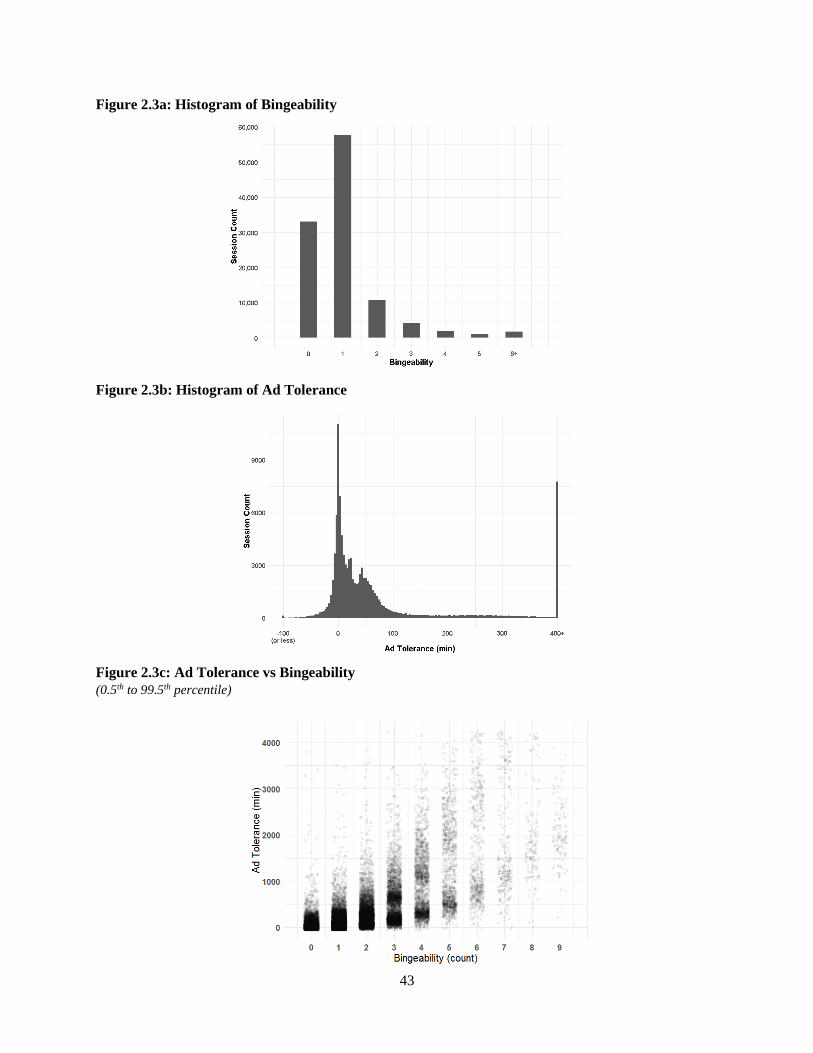
43

Figure 2.3a: Histogram of Bingeability

Figure 2.3b: Histogram of Ad Tolerance

Figure 2.3c: Ad Tolerance vs Bingeability

(0.5th to 99.5th percentile)

44

Figure 2.4c: Partial Dependence of 𝑪�̂� on

Bingeability

(2.5th to 97.5th percentile)

CR hat (X4 hat) (%)

Bin

ge

ab

ility h

at (c

ou

nt)

0.8

0.9

1.0

1.1

1.2

0.2 0.3 0.4 0.5 0.6 0.7

Figure 2.4d: Partial Dependence of 𝑺�̂� on Ad

Tolerance

(2.5th to 97.5th percentile)

SR hat (X1 hat) (min)

Ad

To

lera

nce

ha

t (m

in)

140

145

150

155

4 5 6 7 8

Bingeability Sum (same Show) (count)

Bin

ge

ab

ility h

at (c

ou

nt)

1.0

1.1

1.2

1.3

1.4

1.5

0 5 10 15

Ad Tolerance Sum (same Title) (min)

Ad

To

lera

nce

ha

t (m

in)

200

400

600

800

0 1000 2000 3000

Figure 2.4a: Partial Dependence of Bingeability

on Bingeability Sum (same Show, any Day, any

TOD)

(2.5th to 97.5th percentile)

Figure 2.4b: Partial Dependence of Ad Tolerance

on Ad Tolerance Sum (same Title, any Day, any

TOD)

(2.5th to 97.5th percentile)

45

Figure 2.4e: Partial Dependence of Bingeability on its two most important Ad Targeting Rules

(2.5th to 97.5th percentile)

Figure 2.4f: Partial Dependence of Ad Tolerance on its two most important Ad Targeting Rules

(2.5th to 97.5th percentile)

46

Figure 2.5: Ad Decision Tree

Figure 2.6a: Density of Recommended

Spacing in Holdout 1

(2.5th to 97.5th percentile)

Figure 2.6b: Density of Recommended Spacing in

Holdout 2

(2.5th to 97.5th percentile)

47

81st percentile 86th percentile

Figure 2.7a: Density of Average Observed

Spacing in Holdout 1

(2.5th to 97.5th percentile)

Figure 2.7b: Density of Average Observed

Spacing in Holdout 2

(2.5th to 97.5th percentile)

Figure 2.8a: Density of the Ratio of

Recommended Spacing and Average Observed

Spacing in Holdout 1

(2.5th to 97.5th percentile)

Figure 2.8b: Density of the Ratio of

Recommended Spacing and Average Observed

Spacing in Holdout 2

(2.5th to 97.5th percentile)

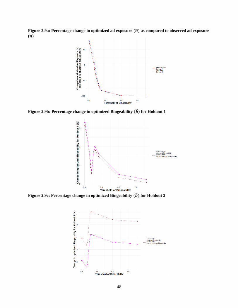
48

Figure 2.9a: Percentage change in optimized ad exposure (�̃�) as compared to observed ad exposure

(𝒏)

Figure 2.9b: Percentage change in optimized Bingeability (�̃�) for Holdout 1

Figure 2.9c: Percentage change in optimized Bingeability (�̃�) for Holdout 2

49

CHAPTER III - Video Influencers: Unboxing the Mystique

3.1 Introduction

Influencers have the capacity to shape the opinion of others in their network (Oxford Reference, 2020).

They were traditionally celebrities (e.g., movie stars and athletes) who leveraged their expertise, fame and

following in their activity domain to other domains. However, 95% of the influencers today, or “social

media stars,” are individuals who have cultivated an audience over time by making professional content

that demonstrates authority and credibility (Creusy, 2016; O'Connor, 2017b). The growth in their

audience(s) has been in part attributed to the fact that influencer videos are seen as “authentic” based on a

perception of high source credibility. The increasing popularity of social media stars has resulted in an

exponential growth of the influencer marketing industry which is expected to reach a global valuation of

$10B in 2020 from $2B in 2017 (Contestabile, 2018). There are now more than 1100 influencer

marketing agencies in the world that allow brands to partner with influencers to promote their products

(Influencer Marketing Hub and CreatorIQ, 2020). These influencers primarily reach their audience(s) via

custom videos that are available on a variety of social media platforms (e.g., YouTube, Instagram, Twitter

and TikTok) (Brooks, 2020). In contrast to conventional advertising videos, influencer videos have

emerged as a distinct medium (see Section 3.3.1 for details explaining why). Despite the rapid emergence

and growth of influencer videos, there is limited research on their design and effectiveness (or indeed

influencer marketing in general). Specifically, little is known about the relationship between video

content and viewer reactions as well as the evolution of these videos over time.31

In this essay, I investigate whether the presence and nature of advertising content in videos is

associated with relevant outcomes (views, interaction rates, and sentiment). There are three main

challenges in carrying out these tasks. First, most data in influencer videos are unstructured. In addition,

these data span different modalities – text, audio and images. This necessitates the use of state-of-the-art

machine learning methods commonly referred to as deep learning. The second challenge arises from the

fact that past approaches in marketing using such methods have typically made a tradeoff between

predictive ability and interpretability. Specifically, such deep learning models predict marketing outcomes

well out-of-sample but traditionally suffer from poor interpretability. On the other hand, deep learning

31 The literature on influencer marketing has primarily looked at the effect of textual content in sponsored blog posts on engagement with the post (Hughes et al., 2019) and the effect of outbound activities to other users on increasing follower base (Lanz et al., 2019).

50

models that use ex-ante handcrafted features obtain high interpretability of the captured relationships but

suffer from poor predictive ability. My “interpretable deep learning” approach handles unstructured data

across multiple modalities (text, audio and images) while avoiding the need to make this trade-off.

Finally, the analysis of unstructured data is computationally very demanding, leading me to use “transfer

learning.” I apply my approach to publicly available influencer videos on YouTube (the platform where

influencers charge the most per post32 (Klear, 2019)).

My approach helps me identify statistically significant relationships between marketing (brand)

relevant outcomes and video elements. The significance of these relationships is supported by a

significant change in attention (importance) paid by the model to these video elements. For the outcomes,

I use publicly available data to develop metrics based on industry practice (Influencer Marketing Hub and

CreatorIQ, 2020) and past research on visual and verbal components of conventional advertising

(Mitchell, 1986). These metrics are # views, engagement (#comments / # views), popularity (# likes / #

views), likeability (# likes / # dislikes) and sentiment (details are in Section 3.3.3). The influencer video

elements I consider are text (e.g., brand names in title, captions/transcript and description), audio (e.g.,

speech, music, etc.), and images (e.g., brand logos, persons, clothes, etc. in thumbnails and video frames).

As noted earlier, the analysis of videos is computationally demanding, so I use a random sample

of 1650 videos in order to interpret the relationship between the video elements and marketing outcomes.

These videos are scraped from 33 YouTube influencers who span 11 product categories and obtain

revenue from brand endorsements.33 A concern with the use of my sample size is the possibility of

“overfitting.” In order to prevent that, I implement transfer learning approaches (which also have the

added benefit of aiding interpretation). Transfer learning approaches, which are applied across all

modalities of text, audio and image data, involve using models pre-trained (at a high monetary and

computational cost) on a separate task with large amounts of data which are then fine-tuned for my

different but related task. This is followed up with an ex-post interpretation step that allows identification

of salient word pieces in text, moments in audio and pixels in images.

The focus on interpretation allows me to document some interesting relationships (based on a

holdout sample) across all three modalities (while controlling for other variables including influencer

fixed effects). First, I find that brand name inclusion, especially in the consumer electronics and video

game categories, in the first 30 seconds of captions/transcript is associated with a significant increase in

attention paid to the brand but a significant decrease in predicted sentiment. Second, human sounds,

mainly speech (without simultaneous music), within the first 30 seconds are associated with a significant

32 An influencer with 1M–3M followers on YouTube can on average earn $125,000 per post - this is more than twice the earnings from a post on

Facebook, Instagram or Twitter (O'Connor, 2017a). 33 My usage of this data falls within the ambit of YouTube’s fair use policy (YouTube, 2020).

51

increase in attention, and their longer duration is associated with a significant increase in predicted views

and likeability. Similarly, music (without simultaneous human sound) within the first 30 seconds is

associated with a significant increase in attention. However, longer music duration is associated with a

significant decrease in predicted engagement, popularity and likeability but a significant increase in

predicted sentiment. Third, larger pictures (of persons as well as clothes & accessories) in five equally

spaced video frames (within the first 30 seconds) are associated with a significant increase in attention

and predicted engagement. Fourth, more animal sounds in the first 30 sec of a video is associated with a

significant increase in attention and a significant increase in predicted likeability. Finally, I also

demonstrate that the focus on interpretability does not compromise the predictive ability of my model.

These results are relevant for multiple audiences. For academics, who may be interested in testing

causal effects, my approach is able to identify a smaller subset of relationships for formal causal testing.

This is done by filtering out more than 50% of relationships that are affected by confounding factors

unassociated with attention (importance) paid to video elements. For practitioners, I provide a general

approach to the analysis of videos used in marketing that does not rely on primary data collection. For

brands, influencers and influencer agencies, my results provide an understanding of the association

between video features and relevant outcomes. Influencers can iteratively refine their videos using my

model and results to improve performance on an outcome of interest. Brands, on the other hand, can

evaluate influencer videos to determine their impact and effectiveness at various levels of granularity

(individual video elements, interactions of elements or holistic influence).

Overall, this essay makes four main contributions. First, to the best of my knowledge, it is the

first essay that rigorously documents the association between advertising content in influencer videos and

marketing outcomes. Second, it presents an interpretable deep learning approach that avoids making a

tradeoff between interpretability and predictive ability. It not only predicts well out-of-sample but also

allows interpretation and visualization of salient regions in videos across multiple data modalities – text,

audio, and images. Third, it generates novel hypotheses between advertising content and a change in the

outcome of interest for formal causal testing as noted above. Finally, it provides a comprehensive, data-

based approach for marketers (and influencers) to assess and evaluate the quality of videos.

The remainder of the chapter is organized as follows. Section 3.2 discusses the related literature

while Section 3.3 describes the institutional setting and data used for analysis. Section 3.4 details the

models for analyzing structured and unstructured data. The results are described in Section 3.5 while the

implications of my approach and findings for practitioners (influencers and marketers) are described in

Section 3.6. Section 3.7 concludes with a discussion of the limitations and directions for future research.

52

3.2. Related Literature

3.2.1 Influencer Marketing

The nascent literature on influencer marketing has so far focused only on textual data (written text,

transcripts, etc.). Hughes et al. (2019) find that high influencer expertise on sponsored blog posts is more

effective in increasing comments below the blog if the advertising intent is to raise awareness versus

increasing trial. However, influencer expertise does not drive an increase in likes of the sponsored post on

Facebook, showing that the type of platform has a role to play in driving engagement. Zhao et al. (2019)

study the audio transcript of live streamers on the gaming platform Twitch, and find that lower values of

conscientiousness, openness and extraversion but higher values of neuroticism are associated with higher

views. Other research, such as Lanz et al. (2019), studies network effects on a leading music platform,

and finds that unknown music creators can increase their follower base by seeding other creators with less

followers than creators who are influencers (with more followers). My focus is to add to this literature by

helping marketers better understand the role of text, audio and image elements in influencer videos.

3.2.2 Unstructured Data Analysis in Marketing via Deep Learning

The use of deep learning methods to analyze unstructured data in the marketing literature has gained

increasing prominence in recent years due to its ability to capture complex non-linear relationships that

help make better predictions on outcomes of interest to marketers. Marketing research on textual data has

used combinations of Convolutional Neural Nets (CNNs) and Long Short-Term Memory Cells (LSTMs)

to predict various outcomes including sales conversion at an online retailer (X. Liu et al., 2019), whether

Amazon reviews are informative (Timoshenko & Hauser, 2019) and sentiment in restaurant reviews

(Chakraborty et al., 2019). Research on image data has also used CNNs but within more complex

architectures such as VGG-16 to predict image quality (S. Zhang et al., 2017) or classify brand images

(Hartmann et al., 2020), Caffe framework to predict brand personality (Liu et al., 2018) and ResNet152 to

predict product return rates (Dzyabura et al., 2018). Past research on both text and image data has found

that deep-learning models that self-generate features have better predictive ability than those that use ex-

ante hand-crafted features (Dzyabura et al., 2018; Liu et al., 2018; X. Liu et al., 2019). While hand-

crafted features suffer from poor predictive ability, they allow interpretability of their effect on the

outcome variable. I avoid ex-ante feature engineering of unstructured data, and instead use ex-post

interpretation, so that I do not need to make a trade-off between predictive ability and interpretability.

Marketing literature has also worked with video data. Pre-trained facial expression classifiers

have been used on images from video frames to infer product preference while shopping (S. Lu et al.,

2016). Similarly, hand-crafted video features have been automatically extracted from images, audio and

text of projects on the crowd funding platform Kickstarter to study their relationship with project success

53

(Li et al., 2019). More recently, there has been research that embeds information from different data

modalities using deep learning methods to create unified multi-view representations. Combinations of

structured data and text have been used to predict business outcomes (Lee et al., 2018); brand logo images

and textual descriptions have been combined to suggest logo features for a new brand (Dew et al., 2019);

and car designs have been combined with ratings data to suggest new designs (Burnap et al., 2019). In my

essay, I do not generate a modality given the other modalities, but instead focus on providing tools to

improve each modality and interpreting the association between multiple modalities (text, images and

audio) and my outcomes of interest.

3.3 Data

3.3.1 Institutional Setting

As noted earlier, influencer videos have emerged as a distinct marketing medium. They are quite different

from conventional advertising videos34 in at least three ways. First, these videos can (and almost always

do) contain information that is unrelated to the sponsoring brand(s). This amount of information varies by

type of video. On the one extreme are “integrated-advertising” videos (e.g., unboxing videos, hauls,

product reviews, etc.) that feature the brand prominently throughout the video; at the other extreme are

the “non-integrated-advertising” videos that feature the name of the sponsored brand only in a part of the

video in the form of mini-reviews, audio shout outs, product placements or brand image displays

(Mediakix, 2020). The latter type of videos includes vlogs, educational videos, gaming videos, etc. that

are not directly related to the sponsoring brand(s).

Second, influencer videos are typically much longer than a standard TV commercial especially on

platforms such as Instagram and YouTube.35 By making longer videos, influencers stand to gain higher

revenue from more mid-roll ad exposures. Furthermore, videos with higher expected watch time are more

likely to be recommended to viewers by the YouTube recommendation algorithm (Covington et al.,

2016). Hence, influencer video content needs to hold viewer attention for a longer duration so that the

video can reach a larger audience, potentially leading to higher word of mouth and content sharing.

Third, influencer videos can be interrupted by traditional ads on YouTube. While YouTube only

allows videos that are eight minutes or longer to have mid-roll ads, pre-roll ads can be a part of all

influencer videos (Google, 2020c). As advertising is the primary source of revenue for influencers

(Zimmerman, 2016), it is common for influencers to enable advertising on their videos, making it likely

34 Past work on characteristics of conventional advertising videos has studied their effect on ad viewing time (McGranaghan et al., 2019; Olney et al., 1991), ad attention (McGranaghan et al., 2019; Teixeira et al., 2010, 2012), ad liking / irritation (Aaker & Stayman, 1990; Pelsmacker & Van

den Bergh, 1999) and purchase intent (Teixeira et al., 2014). 35 The median duration of videos across my sample of 1650 videos is 5.3 min which is 10 times longer than the commonly used commercial duration of 30 seconds (W. Friedman, 2017).

54

for viewers to see traditional-ad-interrupted influencer videos. Given that viewers are exposed to both

influencer conveyed advertising and brand conveyed (traditional) advertising during the same viewing

experience, the cognitive processing of information conveyed from each source can be quite different.

In addition to the above differences, influencer videos are also perceived to have higher source

credibility (Tabor, 2020). Information about the brand is conveyed by an individual with high credibility

and expertise in a related subject area, e.g., review of a beauty product coming from an influencer who

has demonstrated expertise in the beauty industry.

3.3.2 Video Sample

I focus on 120 influencers identified by Forbes in February 201736 (O'Connor, 2017b). These influencers

obtain revenue from brand endorsements and post mostly in English across Facebook, YouTube,

Instagram and Twitter. They span 12 product categories37 (10 influencers in each). I exclude the

influencers in the Kids category as YouTube has disabled comments on most videos featuring children.

Out of the remaining 110 influencers, I exclude influencers who do not have a YouTube channel. I also

use the industry threshold of 1000 followers for a person to be classified an influencer (Maheshwari,

2018) and also exclude one atypical influencer with more than 100M followers. Furthermore, I short-list

those influencers who have at least 50 videos so that I can capture sufficient variation in their activity,

which leaves me with a pool of 73 influencers. From this pool, I randomly choose 3 influencers per

category, which gives a total of 33 influencers38 and a master list of 32,246 videos, whose title and posting

time were scraped using the YouTube Data API v3 in October 2019. In addition, I also record the

subscriber count for each channel at the time of scraping. From this pool of 33 influencers, I randomly

choose 50 public videos for each influencer so that I have a balanced sample of 1650 videos that is

feasible to analyze. Excluding videos in which either likes, dislikes or comments were disabled by the

influencer(s) leaves me with 1620 videos (all scraped in November 2019). Table 3.1 shows the specific

data scraped.

3.3.3 Outcome Variables

The top three ways of measuring influencer marketing success in the industry are conversions, interaction

rates and impressions (Influencer Marketing Hub and CreatorIQ, 2020). Unfortunately, conversion data

are not publicly available. I capture the remaining two (sets of) variables and in addition also capture

sentiment.

36 The criteria used by Forbes to identify these influencers include total reach, propensity for virality, level of engagement, endorsements, and related offline business. 37 The 12 product categories are Beauty, Entertainment, Fashion, Fitness, Food, Gaming, Home, Kids, Parenting, Pets, Tech & Business, and Travel. 38 Three of the randomly chosen influencers had comments disabled on more than 95% of their videos, and hence three other random influencers were chosen in their place from the respective category.

55

(1) Impressions (Views)

Views are important not only to brands, but also to influencers. Higher views help brands increase

exposure levels of their influencer marketing campaign, and help influencers earn more revenue equal to a

55% share of ad CPM39 on YouTube (Rosenberg, 2018). Furthermore, an increase in views is correlated

with an increase in channel subscribers,40 and higher subscriber count allows the influencer to earn higher

CPM rates (Influencer Marketing Hub, 2018) as well as to ex-ante charge higher for a brand collaboration

(Klear, 2019; O'Connor, 2017a).

There are a few different ways in which public view counts are incremented on YouTube. First,

watching a complete pre-roll ad that is 11 to 30 seconds long OR watching at least 30 seconds of a pre-

roll ad that is longer than 30 seconds OR interacting with a pre-roll ad (Google, 2020b). Second, if a pre-

roll ad is skipped OR there is no pre-roll ad OR the complete pre-roll ad is smaller than 11 seconds, then

watching at least 30 seconds of the video (or the full video if it has a shorter duration) has been

historically documented to be the minimum requirement for public view counts to increase (Parsons,

2017).

On average, only 15% of viewers have been typically found to watch 30 seconds of a YouTube

pre-roll ad (Influencer Marketing Hub, 2018). Hence, it is likely that most view counts are incremented

because of viewing the first 30 seconds of video content. As views are exponentially distributed, I show

the distribution of the log of views across my sample of 1620 videos in Figure 3.1. The distribution is

approximately normal and ranges from 3.71 to 17.57 with a median of 11.85 (or 140,000 views).

(2) Interaction Rates

Brands care more about interaction rates than views to not only ex-ante decide on a collaboration but also

to ex-post measure campaign success (Influencer Marketing Hub and CreatorIQ, 2020). Hence, in

addition to using impressions (views) as an outcome of interest, I develop three measures of interaction

rates that are captured in publicly available data: (a) engagement = (# comments / # views), (b) popularity

= (# likes / # views), and (c) likeability = (# likes / # dislikes). While measuring number of comments and

likes is common practice in industry and academia (Dawley, 2017; Hughes et al., 2019), I scale each

measure by (number of) views to develop unique measures that are not highly correlated with views,41 and

hence can be used to compare interaction rates for videos with different levels of views. The third metric,

(# likes / # dislikes), is unique to YouTube because YouTube is the only major influencer platform in the

39 Median ad CPM rates on YouTube are $9.88, and form the primary source of revenue for YouTube influencers (Lambert, 2018; Zimmerman, 2016)

40 Total views for all videos of an influencer channel are highly correlated with subscriber count for the channel across the 33 influencers in my

sample, 𝜌 = 0.91. 41 Across 1620 videos spanning 33 influencers, there is a high correlation between log views and log (comments+1) at 0.91, between log views and log (likes+1) at 0.95 and between log views and log (dislikes+1) at 0.92 (I add 1 to avoid computation of log(0)).

56

US which publicly displays number of dislikes to the content.42 As the three interaction rates are also

exponentially distributed, I take their natural log, and add 1 to avoid computation of log(0) or log(∞): (a)

log engagement = log (comments+1

views), (b) log popularity = log (

likes+1

views), and (c) log likeability = log

(likes+1

dislikes+1). The distribution of the log of the interaction rates for the 1620 videos is shown in Figure

3.2a, 3.2b and 3.2c. The distribution of all three interaction rates is approximately normal. Log

engagement has a median of – 6.21 (or 19 comments per 10K views), log popularity has a median of –

3.81 (or 220 likes per 10K views) while log likeability has a median of 3.99 (or approximately 107 likes

per dislike).

(3) Sentiment

Past work has found that the visual and verbal components of advertising can have an effect on attitude

towards the ad which in turn can have a direct effect on overall brand attitude, including attitude towards

purchasing and using the product (Mitchell, 1986). Hence, it is likely that brands would benefit from

understanding viewer attitude towards the video as it acts as a proxy for sales. I capture attitude towards a

video by measuring the average sentiment expressed in the Top 25 comments below a video using

Google’s Natural Language API. Comments below a YouTube video are by default sorted as ‘Top

comments’ and not ‘Newest first,’ using YouTube’s proprietary ranking algorithm.43 Note that I do not

measure the sentiment in the replies to each of the Top 25 comments because sentiment expressed in the

reply is likely to be sentiment towards the comment and not sentiment towards the video.

The Natural Language API by Google is pre-trained on a large document corpus, supports 10

languages, and is known to perform well in sentiment analysis on textual data (including emojis) in

general use cases (Hopf, 2020). For comments made in a language not supported by the API, I use the

Google Translation API to first translate the comment to English, and then find its sentiment. The

sentiment provided is a score from −1 to +1 (with increments of 0.1), where −1 is very negative, 0 is

neutral and +1 is very positive. I calculate the sentiment of each comment below a video for a maximum

of Top 25 comments, and then find the average sentiment score.44

The distribution of sentiment scores for the 1620 videos is shown in Figure 3.3. It ranges from

−0.9 to 0.9 with a median of 0.34, which I use as a cut-off to divide sentiment in the videos into two

buckets – “positive” and “not positive (neutral or negative).” The large peak at 0 is because of 71 videos

42 Other influencer platforms either do not allow dislikes to content or only allow content to be marked as ‘not interesting’ which is not publicly displayed. 43 Higher ranked comments (lower magnitude) have been empirically observed to be positively correlated with like/dislike ratio of comment,

like/dislike ratio of commenter, number of replies to the comment and time since comment was posted (Dixon & Baig, 2019). Moreover, a

tabulation shows that 99% of comments are made by viewers and not the influencer (who owns the channel) and hence I do not separate the two. 44 As a robustness check, I use Top 50 and Top 100 comments for a random sample of 66 videos (2 videos per influencer) and also explore use of

progressively decreasing weights instead of a simple average. I find that the sentiment calculated using any of these measures is highly correlated

with a simple average of Top 25 comments (𝜌 ≥ 0.88).

57

where viewers do not post any comments (even though comment posting has not been disabled by the

influencer). I assume that if viewers choose to not post comments below a video, then the sentiment

towards the video is neutral (0).

Hence, I have a total of four continuous outcomes and one binary outcome. I find that the Pearson

correlation coefficient between all outcomes ranges from 0.02 to 0.66 with a median of 0.20 (absolute

value) as shown in Table 3.2, indicating that each measure potentially captures different underlying

constructs.

3.3.4 Features

Next, I generate features from the data scraped in Table 3.1 and list them in Table 3.3. As can be seen

from the table, I have 33 fixed effects for channel, 11 fixed effects for category, features for video length,

tags and playlist information, six time-based-covariates and an indicator variable for whether captions are

available for the video. For the video description, a maximum of 160 characters are visible in Google

Search and even fewer characters are visible below a YouTube video before the ‘Show More’ link

(Cournoyer, 2014). Hence, I truncate each description to the first 160 characters as it is more likely to

contribute to any potential association with my outcome variables. Captions are only present in 74% of

videos, and for those videos without a caption, I use Google’s Cloud Speech-to-Text Video Transcribing

API to transcribe the first 30 seconds of the audio file to English.45

I begin by focusing on the first 30 seconds for two reasons.46 First, the minimum duration of video

content that needs to be viewed for an impression to be registered is 30 seconds, and second, higher

computational costs associated with more data in my deep learning models require me to restrict data size

to a feasible amount. Similarly, I restrict the duration of the audio file to the first 30 seconds. I use audio

data in addition to captions/transcript to analyze the presence of other sound elements such as music and

animal sounds. Image data comprise high-resolution images that are 270 pixels high and 480 pixels wide.

These images comprise the thumbnail and video frames at 0 sec (first frame), 7.5 sec, 15 sec, 22.5 sec and

30 sec.47 I restrict my analysis to the first 30 seconds of the video to be consistent with my analysis of text

and audio data, and I consider a maximum of five frames in the first 30 seconds because of computational

constraints of GPU memory that can be achieved at a low cost.

I create two additional structured features from the complete description to use for analysis as the

complete description is not supplied to the Text model. These features are included as they can lead the

45 While most videos have English speech, if the first 30 seconds of audio have only non-English speech or there is only background

music/sound, the transcription process results in an empty file. 65% of the 26% of videos that are transcribed result in an empty file. 46 Note that as part of my robustness checks, I contrast my approach with the use of data from the middle 30 sec and last 30 sec of the video (see

Section 2.5.4). 47 As each video can be recorded at a different frame rate or with variable framing rates, I capture the frame equal to or exactly after the specified time point. For example, a video recorded at a fixed rate of 15 frames/sec will have a frame at 7.46 sec and 7.53 sec but not 7.50 sec - so I record the frame at 7.53 sec in place of 7.50 sec.

58

viewer away from the video. They comprise total number of URLs in description and an indicator for

hashtag in description. The first three hashtags used in the description appear above the title of the video

(if there are no hashtags in the title), and clicking on it can lead the viewer away from the video to another

page that shows similar videos (Google, 2020e).48

3.3.5 Brand Usage

I compile a list of popular global brands and a comprehensive list of brands with offices in USA. Three

lists of Top 100 Global brands in 2019 are obtained from BrandZ, Fortune100 and Interbrand. To this, I

add a list of more than 32,000 brands (with US offices) from the Winmo database. This is further

combined with brand names identified by applying Google’s Vision API - Brand Logo Detection on

thumbnails and video frames (0s, 7.5s, 15s, 22.5s & 30s) in my sample of 1620 videos. From this

combined list, I remove more than 800 generic brand names such as ‘slices,’ ‘basic,’ ‘promise,’ etc. that

are likely to be used in non-brand related contexts. Using regular expressions, I identify a list of 250

unique brands that are used in different text elements of a video: video title, video description (first 160

characters) and video captions/transcript (first 30 sec). The Logo detection API provides a list of 51

unique brands that are used in image elements of the video – thumbnails and video frames. The

percentage of videos that have a brand used in each video element is as follows: title – 11.2%, description

(first 160 characters) – 36.8%, captions/transcript (first 30 sec) – 17.2%, thumbnails – 1.1% and video

frames (across five frames in first 30sec) – 2.6%.49 The distribution of the number of brand mentions in

each text element is shown in Figure 3.4a, and the number of brand logos in each image element is shown

in Figure 3.4b.

I find that brand mentions are most common in the description (first 160 characters), followed by

captions/transcript (first 30 sec), and then video title. Moreover, all text elements typically have only one

brand mentioned once; the observations where two or more brands are mentioned include cases of the

same or a different brand being mentioned again. Similarly, thumbnails and video frames (five equally

spaced frames in the first 30 sec) typically have only one brand logo, but they comprise a very small

percentage of the total videos in my sample. Overall, I find that my sample of influencers allows me to

capture sufficient advertising information in textual data.

Furthermore, the US Federal Trade Commission (FTC) has three main guidelines for influencers.

First, influencers need to disclose information about brand sponsorship in the video itself and not just in

the description of the video. Second, they are advised to use words such as “ad,” “advertisement,”

48 I do not have information on how often a video was recommended to viewers by the YouTube recommendation algorithm. I discuss the potential impact of not observing this feature in Section 2.5.2.4. 49 I do not study brand usage in the Top 25 comments below a video as an outcome variable because only about 5% of the comments across all 1620 videos have a brand mentioned.

59

“sponsored” or “thanks to ‘Acme’ brand for the free product” to indicate a brand partnership. Third, it is

recommended that they disclose brand partnerships at the beginning than at the end of a video (FTC,

2020). Hence, I check for presence of the words “ad/s,” “advertisement/s,” “sponsor/s” or “sponsored” in

the captions/transcript (first 30 sec). 50 I find that less than 1% of videos make such a disclosure in the first

30 seconds.51 While it is known that these influencers obtain revenue from brand endorsements (based on

Forbes’ selection criteria), the lack of disclosure in every sponsored video prevents me from verifying

sponsorship in each video52.

3.4. Model

Deep learning models are especially suited to analyze unstructured data (text, audio and images) as they

can efficiently capture complex non-linear relationships and perform well in prediction tasks (Dzyabura

& Yoganarasimhan, 2018). Figure 3.5a shows the traditional deep learning approach that uses

unstructured data (e.g., images from videos) to predict an outcome variable. Features self-generated by

deep learning models are known to have better predictive ability than ex-ante hand-crafted features passed

to deep learning models (Dzyabura et al., 2018; Liu et al., 2018; X. Liu et al., 2019). This is because ex-

ante feature engineering is unable to neither identify a comprehensive set of important features nor

capture all the underlying latent constructs. However, hand-crafted features allow interpretability of the

captured relationships which is not possible with self-generated features created by traditional deep

learning models.

In Figure 3.5b, I show my “interpretable deep learning” approach that avoids ex-ante feature

engineering and instead uses ex-post interpretation to allow for both good predictive ability of outcomes

and interpretation of the captured relationships. To prevent the model from overfitting when analyzing a

moderate sized dataset, I use transfer learning approaches where a model that is pre-trained on a separate

task with large amounts of data (at a high cost) can be fine-tuned for my different but related task. This

not only helps prevent overfitting but also aids in interpretation of the captured relationships. I use state-

of-the-art model architectures with novel customizations that allow visualization of the captured

relationships. Next, I describe each of the deep (transfer) learning models in more detail.

50 I do not check for the presence of words such as “free” because they are often used in other contexts such as “feel free,” “gluten free,” etc. 51 YouTube also has guidelines for influencers. It requires all channel owners to check a box in video settings that says ‘video contains paid promotion’ if their video is sponsored (Google, 2020d). If this box is checked, a tag – “Includes Paid Promotion” is overlaid on a corner of the video for the first few seconds when the video is played on YouTube. While information about the presence of this “tag” cannot be scraped or downloaded with the video to the best of my knowledge, manually checking different videos on YouTube in my sample reveals that there is little compliance to this requirement. 52 While I do not expect my inability to verify sponsorship in each video to affect my analysis (because the influencers in my sample are known to receive brand sponsorship), this is still a limitation of using publicly available data on YouTube.

60

3.4.1 Text Model

Text data are analyzed using Bidirectional Encoder Representation from Transformers (BERT) (Devlin et

al., 2018), a state-of-the-art NLP model that borrows the Encoder representation from the Transformer

framework (Vaswani et al., 2017). The model is pre-trained using Book Corpus data (800M words) and

English Wikipedia (2,500M words) to predict masked words in text and the next sentence following a

sentence. Devlin et al. (2018) complete the pre-training procedure in four days using four cloud Tensor

Processing Units (TPUs). The BERT model is fine-tuned to capture the association with my five

outcomes using the framework shown in Figure 3.6.

The model converts a sentence into word-piece tokens53 as done by state-of-the-art machine

translation models (Wu et al., 2016). Furthermore, the beginning of each sentence is appended by the

‘CLS’ (classification) token and the end of each sentence is appended by the ‘SEP’ (separation token).

For example, the sentence ‘Good Morning! I am a YouTuber.’ will be converted into the tokens [‘[CLS]’,

‘good’, ‘morning’, ‘!’, ‘i’, ‘am’, ’a’, ‘youtube’, ‘##r’, ‘.’, ‘[SEP]’]. A 768-dimensional initial embedding

learnt for each token during the pre-training phase is passed as input to the model, and is represented by

the vector 𝑥𝑚 in Figure 3.6, where m is the number of tokens in the longest sentence54. The token

embedding is combined with a positional encoder 𝑡𝑚 that codes the position of the token in the sentence

using sine and cosine functions (see Devlin et al. (2018) for details). This is passed through a set of 12

encoders arranged sequentially. The output of the ‘CLS’ token is passed through a feed forward layer that

is initialized with pre-trained weights from the next sentence prediction task, and has a tanh activation

function, i.e. tanh(𝑥) =𝑒𝑥−𝑒−𝑥

𝑒𝑥+𝑒−𝑥. This is followed by the output layer, which has a linear activation

function, i.e. 𝑙𝑖𝑛𝑒𝑎𝑟(𝑥) = 𝑥, for the four continuous outcomes and a sigmoid activation function, i.e.

𝑠𝑖𝑔𝑚𝑜𝑖𝑑(𝑥) = 𝑒𝑥

1+𝑒𝑥 , for the binary outcome sentiment.

In Appendix B.1, I explain the architecture of the Encoders which also contain the self-attention

heads. The self-attention heads help the model capture the relative importance between word-pieces while

forming an association with the outcome of interest. The three main advantages of BERT over

conventional deep learning frameworks such as (Bidirectional) LSTM, CNN and CNN-LSTM that use

word embeddings such as Glove and word2vec are as follows: (1) BERT learns contextual token

embeddings (e.g., the embedding for the word ‘bark’ will change based on the context in which it used,

such that the model can understand whether the word is referring to a dog’s bark or a tree’s outer layer)

(2) The entire BERT model with hierarchical representations is pre-trained on masked words and a next

53 I use the BERT-base-uncased model (that converts all words to lower case and removes accent markers) as compared to the cased model, because the uncased model is known to typically perform better unless the goal is to study case specific contexts such as ‘named entity recognition’ and ‘part-of-speech tagging’. 54 Rare characters including emojis are assigned an ‘UNK’ (unknown) token and sentences shorter than the longest sentence are padded to the maximum length by a common vector.

61

sentence prediction task, thus making it suitable for transfer learning; whereas the conventional models

only initialize the first layer with a word embedding (3) BERT uses a self-attention mechanism that

allows the model to simultaneously (non-directionally) focus on all words in a text instead of using a

sequential process that can lead to loss of information. These advantages are reflected in model

performance when I compare it with conventional models (combinations of CNN and LSTM) in Section

3.5.1.

3.4.2 Audio Model

Audio data are analyzed using the state-of-the-art YAMNet model followed by a Bidirectional LSTM (Bi-

LSTM) model with an attention mechanism, as shown in Figure 3.7. YAMNet takes the Mel-frequency

spectrogram of the audio signal as input and passes it through a MobileNet v1 (version 1) model that is

pre-trained on the AudioSet data released by Google (Gemmeke et al., 2017; Pilakal & Ellis, 2020).

YAMNet predicts sound labels from 521 audio classes55 such as speech, music, animal, etc. corresponding

to each 960ms segment of the audio file. The features from the last layer of the model, corresponding to

the predicted audio classes, are passed through a Bi-LSTM layer with an attention mechanism to capture

the sequential structure of sound. The model is then fine-tuned to capture associations with my five

outcomes.

Next, I explain the model framework in more detail. As mentioned earlier in Section 3.2, I

analyze the first 30 seconds of audio in each video file. Each 30 second audio clip is resampled at 16,000

Hz and mono sound, which results in 480,000 data points for each clip. To summarize the large number

of data points, I generate a spectrogram that spans the frequency range of 125 to 7500Hz (note that the

2000-5000 Hz range is most sensitive to human hearing (Widex, 2016)) over which the YAMNet model

has been pre-trained. This frequency range is then divided into 64 equally spaced Mel bins on the log

scale, such that the sounds of equal distance on the scale also sound equally spaced to the human ear.56

Each segment of 960ms from the spectrogram output, i.e., 96 frames of 10ms each with overlapping

patches (that have a hop size of 490ms) to avoid losing information at the edges of each patch is passed as

input to the MobileNet v1 architecture. The MobileNet v1 (explained in more detail in Appendix B.2)

processes the spectrogram through multiple mobile convolutions which results in 521 audio class

predictions across 60 moments (time steps) in the clip. The <521x60 > dimensional vector is then passed

as input to the Bi-Directional LSTM layer with an attention mechanism (explained in more detail in

Appendix B.2). This layer is made Bidirectional to allow it to capture the interdependence between

55 The AudioSet data has more than 2 million human-labelled 10 sec YouTube video soundtracks (Gemmeke et al., 2017). Pilakal and Ellis (2020) remove 6 audio classes (viz. gendered versions of speech and singing; battle cry; and funny music) from the original set of 527 audio classes to avoid potentially offensive mislabeling. YAMNet has a mean average precision of 0.306. 56 The spectrogram uses the pre-trained Short-Term Fourier Transform window length of 25ms with a hop size of 10ms that results in a 2998 x 64 (time steps x frequency) vector corresponding to 30 seconds of each audio clip.

62

sequential audio segments from both directions. For example, the interdependence between the sound of a

musical instrument at 5 seconds and the beginning of human speech at 15 seconds can be captured by the

model bidirectionally. I adopt the attention mechanism used for neural machine translation by Bahdanau

et al. (2014) to help the Bi-LSTM model capture the relative importance between sound moments in order

to form an association with an outcome of interest. The output of the Bi-LSTM with attention mechanism

is passed through an output layer which has linear activations for the continuous outcome and sigmoid

activation for the binary outcome. I compare the performance of this model framework (Model 3) with a

model devoid of the attention mechanism (Model 2) and a model devoid of both the attention mechanism

and MobileNet v1 (Model 1), in Section 3.5.157.

3.4.3 Image Model

Individual images are analyzed using the state-of-the-art image model – EfficientNet-B7 (Tan & Le,

2019) that has been pre-trained with “noisy student weights”58 (Xie et al., 2019). This model not only has

a high Top-5 accuracy on ImageNet (98.1%) but is also known to better capture salient regions of images

as it uses compound scaling. It is also a relatively efficient model that uses only 66M parameters (and

hence the name EfficientNet) as compared to other high performing models that use 8x times the number

of parameters (Atlas ML, 2020). All my images (frames) are at a high resolution of 270 by 480 pixels

which is the largest common resolution size available across all thumbnails and video frames in the

dataset. Thumbnail images are passed as input to one EfficientNet-B7, and its final layers are fine-tuned

to capture relationships with an outcome. The architecture of the EfficientNet-B7, whose main building

block is the Mobile Inverted Bottleneck Convolution, is explained in detail in Appendix B.3. I compare

the performance of the (pre-trained) EfficientNet-B7 with a 4-layer CNN model in Section 3.5.1.

As mentioned in Section 3.3, I analyze a maximum of five video frames in the first 30 seconds of

each video, i.e., frames at 0s (first frame), 7.5s, 15s, 22.5s and 30s. Each image frame 𝑖 = 1 to 𝑚, where

𝑚 has a maximum value of 5, is passed through an EfficientNet-B7 model, and then the outputs from all

the models are combined before passing it through an output layer. This is illustrated using the diagram in

Figure 3.8.

57 New methods to recognize speech from unlabeled audio data (using unsupervised learning) such as wav2vec have also been recently developed which can be used in applications where labelled data is not available (Schneider et al., 2019). 58 Xie et al. (2019) learn these weights by first pre-training the model on more than 1.2M labelled images from the ImageNet dataset (Russakovsky et al., 2015), and then use this trained model as a teacher to predict labels for a student model with 300M unlabeled images from the JFT Dataset (Xie et al., 2019). The two models are then combined to train a larger student model which is injected with noise (e.g., dropout, stochastic depth and data augmentation), and is then used as a teacher to predict labels for the original student model. This process is then iterated a few times to produce the EfficientNet-B7 model with pre-trained weights.

63

I compare the performance of four different ‘combination architectures’ that combine the outputs

from each EfficientNet-B7. Two of the architectures are the best performing ones in Yue-Hei Ng et al.

(2015), namely Bi-LSTM59 and Max Pooling followed by Global Average Pooling (Max-GAP). The

remaining two architectures are variants not tested by Yue-Hei Ng et al. (2015), namely Global Average

Pooling followed by Max Pooling (GAP-Max) and Concatenation of Global Average Pooling (C-GAP).

The Bi-LSTM architecture captures sequential information across the video frames, while the remaining

three architectures preserve the spatial information across the video frames. The output of the

combination architecture is passed through an output layer which has linear activations for the continuous

outcome and softmax activation for the binary outcome. I explain the combination architectures in more

detail in Appendix B.3.

3.4.4 Combined Model

I use the framework shown in Figure 3.9 to combine information from each of the unstructured models

with the structured features, 𝑋𝑖𝑡, listed earlier in Table 3.3. The predicted outcome values, �̂�𝑖𝑡 for video 𝑡

by influencer 𝑖, from the best performing model for each unstructured feature, are fed into the combined

model in addition to the structured features, 𝑋𝑖𝑡. This can also be represented by the following equation:

𝑌𝑖𝑡 = 𝑔 (𝑋𝑖𝑡 , �̂�𝑖𝑡𝑇𝑖𝑡𝑙𝑒 , �̂�𝑖𝑡𝐷𝑒𝑠𝑐𝑟𝑖𝑝𝑡𝑖𝑜𝑛 , �̂�𝑖𝑡𝐶𝑎𝑝𝑡𝑖𝑜𝑛/𝑇𝑟𝑎𝑛𝑠𝑐𝑟𝑖𝑝𝑡 , �̂�𝑖𝑡𝐴𝑢𝑑𝑖𝑜, �̂�𝑖𝑡𝑇ℎ𝑢𝑚𝑏𝑛𝑎𝑖𝑙 , �̂�𝑖𝑡𝑉𝑖𝑑𝑒𝑜 𝐹𝑟𝑎𝑚𝑒𝑠) + 𝜖𝑖𝑡

(3.1)

where 𝑌𝑖𝑡 is the observed outcome for video 𝑡 by influencer 𝑖, 𝑔 is the combined model used and 𝜖𝑖𝑡 is the

error term. I test the performance of seven different combined models in Section 3.5.1. The combined

models comprise four commonly used linear models – OLS60, Ridge Regression, LASSO and Elastic Net,

and three non-linear models – Deep Neural Net, Random Forests and Extreme Gradient Boosting

(XGBoost) – that are known to capture non-linear relationships well.

3.5 Results

In this section, I first detail the results on prediction and then on interpretation. I then dig deeper

to see if I find patterns consistent with influencers “learning” about what makes their videos more

engaging. I also carry out a robustness check where I estimate my model on video slices from the middle

and end of videos as opposed to the beginning.

59 While Yue-Hei Ng et al. (2015) use the LSTM approach, I use the Bidirectional LSTM (Bi-LSTM) as it can only perform better than LSTM. 60 I drop the multicollinear category fixed effects in OLS. I retain these fixed effects in the other models so that I can capture their relative

importance with influencer fixed effects.

64

3.5.1 Prediction Results

I divide my random sample of 1620 videos into a 60% training sample (972 videos), 20% validation

sample (324 videos) and 20% holdout sample (324 videos). I train the model on the training sample, tune

the number of steps of Adam gradient descent on the validation sample, and then compute model

performance on the holdout sample.61 First, I compare the predictive performance of each model with

benchmarks models for the continuous outcome (views) and binary outcome (sentiment), and then apply

the best performing model on the other three continuous outcomes (interaction rates).62 In Appendix B.4, I

compare my models with various benchmarks used in marketing literature. The Text model (BERT)

performs better than benchmarks such as LSTM, CNN (X. Liu et al., 2019), CNN-LSTM (Chakraborty et

al., 2019) and CNN-Bi-LSTM. The Audio model (YAMNet+Bi-LSTM+Attention) performs better than

benchmark models devoid of the attention mechanism, thus demonstrating the benefit of capturing

relative attention weights. The Image model (EfficientNet-B7) performs better than a conventional 4-

layer CNN. Furthermore, the Bi-LSTM architecture which captures the sequential information from video

frames performs better than other models that capture only spatial information.63 Overall, I demonstrate

that my models perform better than benchmark predictive models in the marketing literature and thus I do

not compromise on predictive ability.

I also compared the performance of BERT with RoBERTa (Robustly Optimized BERT

Pretraining Approach) (Y. Liu et al., 2019). RoBERTa is pre-trained for a longer duration, on bigger

batches, with more data, on longer sequences, and with dynamic masking. I find that the change in out-of-

sample predictive performance between RoBERTa and BERT ranges from -5% to +8% for all five

outcomes using Title or Transcript. Overall, as performance change can be either negative or positive,

RoBERTa does not always perform better than BERT in this setting. Furthermore, as the percentage

differences are small, this suggests that the performance of both models is comparable in my setting and

are not significantly different from each other. I was unable to analyze description (first 160c) with the

RoBERTa model using a 16GB GPU because of increase in computational complexity. The number of

tokens required to represent the longest first 160 characters of description increased to 314 in RoBERTa

from 124 in BERT. This is primarily due to increase in tokens used to represent emojis – while BERT

assigned an “unknown token” to each emoji, RoBERTa assigns two or more tokens for each emoji.

61 I carry out my analysis using one NVIDIA Tesla P100 GPU (with 16GB RAM) from Google. The predictions results are found by averaging the results over three run times of the model. It is important to note that the results are very close to each other during each run time which demonstrates robustness of the results to the random starting weights chosen by the model during each run time. Other parameters – learning rate and batch size – are chosen such that the model results are obtained in a reasonable run time of less than 30 minutes. 62 I do not use a Multi-Task Learning (MTL) approach to simultaneously predict all five outcomes for two reasons. First, my final goal is to interpret the relationship between each individual outcome and video data (detailed in Section 5.2), which will not be possible with a MTL approach. Second, there is low to moderate correlation between all five outcomes as shown earlier in Table 2.2, which suggests that each outcome is capturing different underlying constructs. 63 I also find that using five frames results in slightly improved performance than a model that uses only three or two frames.

65

However, given the results obtained with Title (which has emojis) does not substantially change between

RoBERTa and BERT, I do not expect the results with Description (160c) to substantially change between

the two models as well. As the predictive results of RoBERTa are not always better than BERT, I do not

analyze the results from RoBERTa for interpretation in Section 3.5.2.

Table 3.4 summarizes the results from the best performing models for each component of

unstructured data, which are now applied to all five outcomes. The Text model (BERT) predicts all the

continuous outcomes with a low RMSE, (e.g., Title can be used to predict views within an average RMSE

range of ±𝑒1.66 = ± 5.26 views) and the binary outcome with moderately high accuracy (e.g., Title can

predict sentiment with an accuracy of 72%). The Audio model can make predictions at a slightly poorer

level of performance than the Text model. The Thumbnail model is unable to predict the continuous

outcomes as well as the Text and Audio Model but performs better than the Audio model in predicting

sentiment. The Video Frames model performs better than the Thumbnail model but poorer than Audio

and Text models in predicting the continuous outcomes but performs comparably with the Thumbnail

model in predicting sentiment. Overall, the prediction results show low RMSE that ranges from 0.71 to

3.09 when predicting the (log transformed) continuous outcomes (views, engagement, popularity and

likeability) and moderately high accuracies ranging from 65% to 72% when predicting sentiment.

The results of the Combined Model used in Section 3.4.4 demonstrate that Ridge Regression has

the best performance on the holdout sample for all the continuous outcomes (lowest RMSE) and also the

binary outcome (highest accuracy) (see Appendix B.4 for details). This suggests that structured features

do not have substantial non-linear interactions with each other or with the predictions from the Text,

Audio and Image models64.

Moreover, I find that the combined model of Ridge Regression has lower RMSE or higher

accuracy than the results of the individual models in Table 3.4, suggesting that the holistic influence of all

features is better than the individual influence of each unstructured feature. Next, I take the magnitude of

each estimated coefficient from the Ridge Regression model applied on the training sample and scale it by

the sum of the magnitude of all coefficient values which gives me the percentage contribution of each

feature. I thus capture the relative importance or predictive power of a feature for each of the outcomes of

interest while controlling for the presence of other features. The importance of each feature set is shown

in Table 3.5.65

64 Note that the features used in Ridge Regression do not include interactions. An alternative reason for Ridge Regression performing better than non-linear models could be the limited number of structured features used in the model (as shown in Tab 3.3). Addition of more structure features (if available) may result in non-linear models performing better at prediction.

65 Note that I scale all the features by their 𝐿2 norm before running the model so that I can make relative comparisons. Also, I sum up the

coefficient values that lie within a class (e.g. sum up the coefficient values of influencer fixed effects, sum up the coefficient values of features of

playlist information, etc.) to get an overall picture of the contribution of a class of features in predicting an outcome of interest.

66

I highlight the unstructured features in gray. Title, description (first 160 characters) and

captions/transcript (first 30 sec) contribute relatively more than the other unstructured features in

predicting all five outcomes. The ordering of relative influence, where I control for the presence of other

structured and unstructured features, is the same as my finding in Table 3.4 where I do not control for the

presence of other features. However, the results of the combined model especially allow me to make

relative comparisons between outcomes. I find that title and description (first 160 characters) contribute

most towards predicting engagement; captions/transcript (first 30s) contribute most towards predicting

popularity, whereas thumbnail, audio (first 30s) and video frames (0s,7.5s,15s,22.5s,30s) contribute most

towards predicting sentiment.

3.5.2 Interpretation Results

In this section, I interpret the best performing transfer learned deep learning models in order to identify

important video elements that can potentially have a causal impact on marketing outcomes. I interpret

results using predictions on the holdout sample, and not the training sample, so that the identified

relationships are more likely to generalize out-of-sample. On the holdout sample, I focus on the following

video elements in unstructured data. First, I focus on brand presence in text as it is of interest to brand

sponsors and because past literature on influencer videos has not studied this (as mentioned earlier in

Section 3.2.1). Second, I study audio elements such as duration of speech, music, and animal sounds. As

past advertising literature has found that ads featuring animals and those using voice-over and music

reduce irritation towards the ad (Pelsmacker & Van den Bergh, 1999), I study the role of these audio

elements in influencer videos. Similarly, I study image elements such as size of brand logos, clothes and

accessories and persons as it is of interest to brand sponsors and has not been studied in past influencer

marketing literature.

I divide my interpretation strategy into two steps to eliminate spurious relationships and visually

illustrate this in Figure 3.10. In Step 1 (Attention or Importance), I first capture the attention weights

(gradients) attributed to the video elements in each deep learning model while making predictions on a

holdout sample. For example, the predicted attention weight for token 𝑗 in the captions in video 𝑡 capture

the relative weight attributed to that token in video 𝑡 while predicting an outcome. These weights for

video 𝑡 sum up to one, and hence capture the relative importance for each token. A higher attention

weight can be thought of in econometrics terms as capturing the strength of the marginal effect. Hence, a

token with higher attention weight would capture more of the variance in the outcome. I regress these

attention weights on the video elements to determine whether the presence of a video element has a

significant positive relationship (significant relationship for gradients) with the predicted attention weight.

This allows me to identify important elements. However, finding important elements here need not

67

indicate that they have a causal impact on the outcome because of potential spurious relationships

captured by the model (Vashishth et al., 2019). Hence, the captured associations need not always be

intrinsically valid.

In Step 2 (Correlation), I regress the predicted outcome from each deep learning model on the

video elements. I use predicted outcomes and not observed outcomes in the holdout sample because the

predicted outcomes have been influenced by the attention weights (gradients) and hence are comparable

with the analysis in Step 166. However, finding significant relationships here need not mean that the

elements are important in order to predict the outcome because of confounds unassociated with attention

paid to video elements. Hence, I find relationships that fall at the intersection of Step 1 and Step 2. Doing

so allows me to identify relationships between video elements and outcomes that are also supported by a

significant change in attention to video elements. Thus, I am able to generate a smaller set of hypotheses

for formal causal testing67. Next, I detail my interpretation strategy using the results from the Text, Audio

and Image models.

3.5.2.1 Interpretation: Text Model

I average the output across all the attention heads in the last encoder of the BERT model, which results in

an attention vector of dimension <324, 𝑘, 𝑘> where 324 is the number of observations in the holdout

sample, and <𝑘,𝑘> corresponds to 𝑘 weights for 𝑘 tokens, where 𝑘 equals the maximum number of

tokens for a covariate type – title, description (first 160 characters) or captions/transcript (first 30s). As

mentioned in Section 3.4.1, the first token for each example is the ‘CLS’ or classification token. I am

interested in the attention weights corresponding to this token because the output from this token goes to

the output layer (as shown earlier in Figure 3.6). Thus, I get at an attention weight vector of dimension

<324, 𝑘>, where each observation has 𝑘 weights corresponding to the ‘CLS’ token. Note that the sum of

the relative attention weights for each observation is one.

After finding the predicted attention weights in the holdout sample, I implement Step 1 where I

run a regression of the predicted attention weights on brand presence to answer the following question:

1) Brand Attention: Do brand names receive more attention?

log(𝐴𝑡𝑡𝑒𝑛𝑡𝑖𝑜𝑛𝑊𝑒𝑖𝑔ℎ𝑡𝑖𝑡𝑗) = 𝛼𝑖 + 𝛾𝑋𝑖𝑡 + 𝛽1(𝐵𝐼𝑇𝑖𝑡𝑗) + 𝛽2(𝐿𝑂𝑇𝑋𝑖𝑡 ) + 𝛽3(𝑇𝑃𝑖𝑡𝑗) + 𝜖𝑖𝑡𝑗 (3.2)

where, 𝐴𝑡𝑡𝑒𝑛𝑡𝑖𝑜𝑛𝑊𝑒𝑖𝑔ℎ𝑡𝑖𝑡𝑗 is the weight for token 𝑗 (excluding ‘CLS’,’SEP’ and padding tokens) in

video 𝑡 made by influencer 𝑖, 𝛼𝑖 is influencer fixed effect, 𝑋𝑖𝑡 is the same vector of structured features

66. Furthermore, the low RMSE values and moderately high accuracies (found in Section 2.5.1) do not preclude the use of predicted outcomes for analysis. 67 Alternative approaches for interpretation such as LIME (Local Interpretable Model Agnostic Explanations) can be used when engineered features are supplied ex-ante to a deep learning model. However, as I am carrying out ex-post interpretation, LIME cannot be applied in this case.

68

used earlier in equation (3.1) 68, and 𝜖𝑖𝑡𝑗 is the error term. 𝐵𝐼𝑇𝑖𝑡𝑗 is a ‘Brand Indicator in Token’ variable

denoting whether token 𝑗 used by influencer 𝑖 in video 𝑡 is a part of a brand name, 𝐿𝑂𝑇𝑋𝑖𝑡 is the Length

Of Text in video 𝑡 made by influencer 𝑖, and 𝑇𝑃𝑖𝑡𝑗 is the Token Position of token 𝑗 used by influencer 𝑖 in

video 𝑡. In addition to studying main effects in equation (3.2), I also study interaction effects in Appendix

B.5.

While equation (3.2) helps study the effect of brand presence on attention to the token, I also

want to study the association between brand presence and the five outcomes of interest. Now, the

predicted outcomes from the BERT model would have been influenced by the relative attention weights

between words. Hence, in Step 2, I run a regression to answer the following question:

2) Brand Presence: Is brand presence associated with the predicted outcome?

𝑃𝑟𝑒𝑑𝑖𝑐𝑡𝑒𝑑𝑂𝑢𝑡𝑐𝑜𝑚𝑒𝑖𝑡 = 𝛼𝑖 + 𝛾𝑋𝑖𝑡 + 𝛽1(𝐵𝐼𝑇𝑋𝑖𝑡) + 𝛽2(𝐿𝑂𝑇𝑋𝑖𝑡) + 𝜖𝑖𝑡 (3.3)

where, 𝐵𝐼𝑇𝑋𝑖𝑡 is a ‘Brand Indicator in Text’ variable denoting whether the text in video 𝑡 by influencer 𝑖

has a brand, and 𝜖𝑖𝑡 is the error term. I study interaction effects in Step 2 in Appendix B.5. The values of

the coefficients of interest in each of the above equations are shown in Table 3.6.

The table reflects results corresponding to each type of unstructured text data – Title, Desc (first

160 characters of description) and Tran (first 30 sec of captions/transcript), and the model for each of the

five outcomes – views, sentiment, engagement, popularity and likeability. The values in the table reflect a

percent change in the non-log-transformed outcome (e.g., views and not log(views)) when a covariate is

present.69 Significant results are suffixed by * (𝑝 < 0.05) and weakly significant results (0.05 ≤ 𝑝 < 0.1)

are suffixed by W.

I highlight the cells in gray that correspond to both (a) a positive and significant effect on

attention weights and (b) a significant effect associated with the predicted outcome. Such a two-step

comparison allows me to filter out significant relationships confounded by factors unrelated to brand

attention. Doing so allows me to identify relationships that are more likely to have causal effects when

tested in the field. I find two main effects that are significant in both steps. First, brand mention in

description (first 160 characters) is associated with an increase in attention and an increase in predicted

views. Second, brand mention in captions/transcript (first 30s) is associated with an increase in attention

but negatively associated with predicted sentiment. However, I do not find any significant evidence to

show that the effect of brand mentions can vary based on length of text or its position in the text (see

Appendix B.5).

68 Note that I do not include category fixed effects in the linear regression to avoid multicollinearity with influencer fixed effects. 69 Note that I run a logistic regression for sentiment instead of a linear regression (in Section 2.5.2.1, 2.5.2.2 and 2.5.2.3).

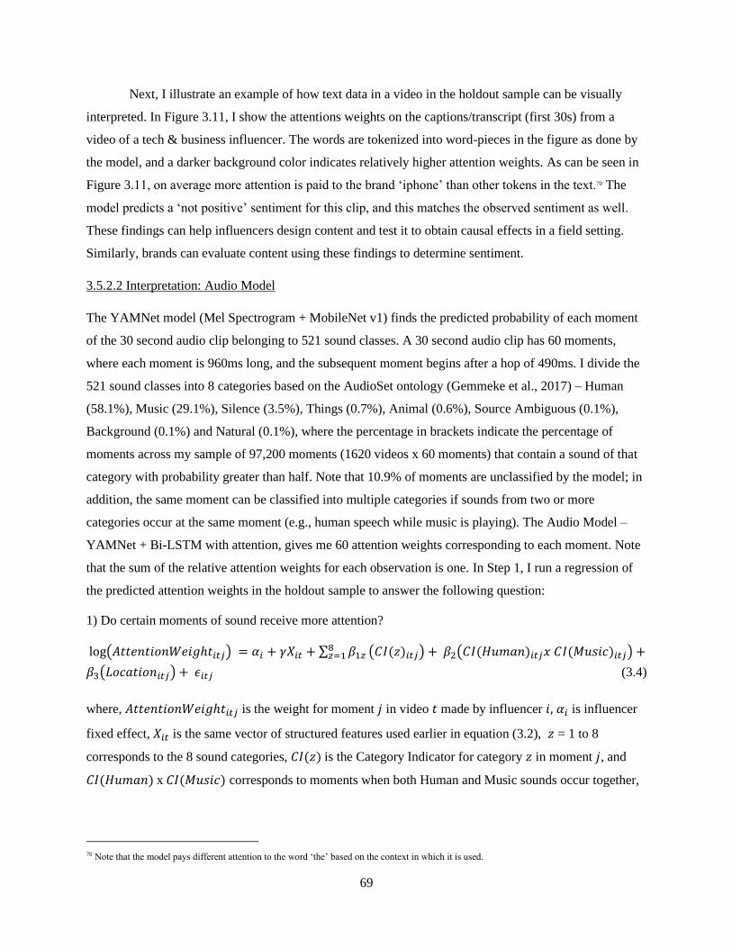
69

Next, I illustrate an example of how text data in a video in the holdout sample can be visually

interpreted. In Figure 3.11, I show the attentions weights on the captions/transcript (first 30s) from a

video of a tech & business influencer. The words are tokenized into word-pieces in the figure as done by

the model, and a darker background color indicates relatively higher attention weights. As can be seen in

Figure 3.11, on average more attention is paid to the brand ‘iphone’ than other tokens in the text.70 The

model predicts a ‘not positive’ sentiment for this clip, and this matches the observed sentiment as well.

These findings can help influencers design content and test it to obtain causal effects in a field setting.

Similarly, brands can evaluate content using these findings to determine sentiment.

3.5.2.2 Interpretation: Audio Model

The YAMNet model (Mel Spectrogram + MobileNet v1) finds the predicted probability of each moment

of the 30 second audio clip belonging to 521 sound classes. A 30 second audio clip has 60 moments,

where each moment is 960ms long, and the subsequent moment begins after a hop of 490ms. I divide the

521 sound classes into 8 categories based on the AudioSet ontology (Gemmeke et al., 2017) – Human

(58.1%), Music (29.1%), Silence (3.5%), Things (0.7%), Animal (0.6%), Source Ambiguous (0.1%),

Background (0.1%) and Natural (0.1%), where the percentage in brackets indicate the percentage of

moments across my sample of 97,200 moments (1620 videos x 60 moments) that contain a sound of that

category with probability greater than half. Note that 10.9% of moments are unclassified by the model; in

addition, the same moment can be classified into multiple categories if sounds from two or more

categories occur at the same moment (e.g., human speech while music is playing). The Audio Model –

YAMNet + Bi-LSTM with attention, gives me 60 attention weights corresponding to each moment. Note

that the sum of the relative attention weights for each observation is one. In Step 1, I run a regression of

the predicted attention weights in the holdout sample to answer the following question:

1) Do certain moments of sound receive more attention?

log(𝐴𝑡𝑡𝑒𝑛𝑡𝑖𝑜𝑛𝑊𝑒𝑖𝑔ℎ𝑡𝑖𝑡𝑗) = 𝛼𝑖 + 𝛾𝑋𝑖𝑡 + ∑ 𝛽1𝑧8𝑧=1 (𝐶𝐼(𝑧)𝑖𝑡𝑗) + 𝛽2(𝐶𝐼(𝐻𝑢𝑚𝑎𝑛)𝑖𝑡𝑗𝑥 𝐶𝐼(𝑀𝑢𝑠𝑖𝑐)𝑖𝑡𝑗) +

𝛽3(𝐿𝑜𝑐𝑎𝑡𝑖𝑜𝑛𝑖𝑡𝑗) + 𝜖𝑖𝑡𝑗 (3.4)

where, 𝐴𝑡𝑡𝑒𝑛𝑡𝑖𝑜𝑛𝑊𝑒𝑖𝑔ℎ𝑡𝑖𝑡𝑗 is the weight for moment 𝑗 in video 𝑡 made by influencer 𝑖, 𝛼𝑖 is influencer

fixed effect, 𝑋𝑖𝑡 is the same vector of structured features used earlier in equation (3.2), 𝑧 = 1 to 8

corresponds to the 8 sound categories, 𝐶𝐼(𝑧) is the Category Indicator for category 𝑧 in moment 𝑗, and

𝐶𝐼(𝐻𝑢𝑚𝑎𝑛) x 𝐶𝐼(𝑀𝑢𝑠𝑖𝑐) corresponds to moments when both Human and Music sounds occur together,

70 Note that the model pays different attention to the word ‘the’ based on the context in which it is used.

70

and 𝐿𝑜𝑐𝑎𝑡𝑖𝑜𝑛 corresponds to location of the moment within the 60 moments of the audio clip, and 𝜖𝑖𝑡𝑗 is

the error term.

Next in Step 2, I examine whether these moments of sound have a significant effect on each outcome.

I use the predicted outcomes from the Audio model as they would have been influenced by the relative

attention weights between moments. I run a regression to answer the following question:

2) Are sound durations of certain sound categories associated with the predicted outcome?

𝑃𝑟𝑒𝑑𝑖𝑐𝑡𝑒𝑑𝑂𝑢𝑡𝑐𝑜𝑚𝑒𝑖𝑡 = 𝛼𝑖 + 𝛾𝑋𝑖𝑡 +∑ 𝛽1𝑧8𝑧=1 (𝑆𝑢𝑚 𝑜𝑓 𝐶𝐼(𝑧)𝑖𝑡) +

𝛽2(𝑆𝑢𝑚 𝑜𝑓 𝐶𝐼(𝐻𝑢𝑚𝑎𝑛) 𝑥 𝐶𝐼(𝑀𝑢𝑠𝑖𝑐)𝑖𝑡) + 𝛽3(𝐵𝑟𝑎𝑛𝑑 𝐼𝑛𝑑𝑖𝑐𝑎𝑡𝑜𝑟 𝑖𝑛 𝐴𝑢𝑑𝑖𝑜𝑖𝑡) + 𝜖𝑖𝑡 (3.5)

where, 𝑆𝑢𝑚 𝑜𝑓 𝐶𝐼(𝑧)𝑖𝑡 corresponds to the sum of the Category Indicator for 𝑧 across the first 60

moments in video 𝑡 made by influencer 𝑖, and 𝑆𝑢𝑚 𝑜𝑓 𝐶𝐼(𝐻𝑢𝑚𝑎𝑛) 𝑥 𝐶𝐼(𝑀𝑢𝑠𝑖𝑐)𝑖𝑡 finds the total

duration when human and music sounds occur together, 𝐵𝑟𝑎𝑛𝑑 𝐼𝑛𝑑𝑖𝑐𝑎𝑡𝑜𝑟 𝑖𝑛 𝐴𝑢𝑑𝑖𝑜𝑖𝑡 borrows the

textual information in captions/transcript (first 30 sec) and acts as an indicator for whether a brand was

mentioned in the audio clip, and 𝜖𝑖𝑡 is the error term. The results for the coefficients in each of the above

equations are shown in Table 3.7. As three sound classes – Source Ambiguous, Background and Natural

are present in only 0.1% of moments, I only use them as controls and hence their coefficients are not

reported in the table. The values in the table reflect a percent change in the non-log-transformed outcome

when a covariate is present (equation (3.4)) or increases by one unit (equation (3.5)).

As done in Section 3.5.2.1, I highlight the cells in gray that correspond to both (a) a positive and

significant effect on attention weights and (b) a significant effect on predicted outcome. This allows me to

filter out significant relationships affected by confounds unassociated with an increase in attention to

audio moments. I find nine significant results. First, human sounds (without simultaneous music) are

associated with an increase in attention, and their longer durations are associated with higher predicted

views and likeability. Second, music (without simultaneous human sounds) is associated with an increase

in attention, and its longer duration is associated with lower predicted engagement, popularity and

likeability but higher predicted sentiment. Last, animal sounds are associated with an increase in

attention, and their longer durations are associated with higher predicted sentiment and likeability. In

addition, I also find that brand presence (in first 30 seconds of audio) is associated with lower predicted

sentiment (while controlling for duration of each class of sound), thus complementing my similar finding

with the Text Model. Thus, I identify significant relationships between sounds and outcomes that are

supported by significant increase in attention paid to audio moments.

71

Next, I illustrate an example of how attention paid to audio moments in a video in the holdout

sample can be visually interpreted. I focus on the relationship between speech and music. In Figure 3.12, I

show the first 30 seconds of the audio clip of a travel influencer using four sub plots. The first plot shows

the variations in the amplitude of the 30 second audio wave (sampled at 16 KHz) followed by the

spectrogram of the wave where brighter regions correspond to stronger (or louder) amplitudes. Next, I

show the interim output of the Audio model with the top 10 sound classes at each moment in the audio,

where the darker squares indicate higher probability of observing a sound of that class at that moment

(Pilakal & Ellis, 2020). The last plot displays the attention weights corresponding to each moment in the

audio clip, where the darker squares indicate higher relative attention placed on that moment while

forming an association with the outcome sentiment. As can be seen in the figure, relatively more attention

is directed to moments where there is music but no simultaneous speech. The model predicts a positive

sentiment for this clip, and this matches the observed sentiment as well.

3.5.2.3 Interpretation: Image Model

The salient parts of the images that are associated with an outcome of interest are visualized through

gradient based activation maps (cf. Selvaraju et al., 2017). Gradients are found by taking the derivative

between the continuous outcome (or class of predicted outcome for sentiment) and the output of the

activation layer after the last convolution layer in the EfficientNet-B7 model. However, unlike Selvaraju

et al. (2017), I do not apply the ReLU (Rectified Linear Unit) activation on the gradient values as I would

like to retain negative gradient values for interpretation. In the Video Frame model, this process is carried

out in each EfficientNet-B7 model corresponding to each video frame. Areas of the image with positive

gradients correspond to regions that are positively associated with continuous outcomes and the predicted

class of sentiment. To systematically identify and summarize the salient regions in thumbnails and video

frames, I use Google’s Cloud Vision API to detect objects and brand logos71 in the images in the holdout

sample. The API returns the vertices of the identified item which allows me to create a rectangular

bounding box to define its area. Next, I divide the identified objects into six categories – Persons (44.2%),

Clothes & Accessories (30.9%), Home & Kitchen (11.0%), Animal (6.0%), Other Objects (3.7%) and

Packaged Goods (1.9%); I let Brand Logos (2.3%) be the seventh category. The percentage in brackets

indicates the percentage of items in that category out of a total of 4066 items (3973 objects + 93 brand

logos) identified across 1944 frames in the holdout sample (324 videos x (1 thumbnail frame + 5 video

frames)). In Step 1, I run a regression of the predicted gradient values in the holdout sample to answer the

following question:

71 I use a 70% confidence level of the Vision API to detect objects and a 90% confidence level to detect brand logos to be conservative in my estimates.

72

1) Is size of objects/brand logos associated with mean gradient over its area?

𝑀𝑒𝑎𝑛𝐺𝑟𝑎𝑑𝑖𝑒𝑛𝑡𝑉𝑎𝑙𝑢𝑒𝑠𝑖𝑡𝑧 = 𝛼𝑖 + 𝛾𝑋𝑖𝑡 + 𝛽𝐼𝑡𝑒𝑚𝑆𝑖𝑧𝑒𝑖𝑡𝑧 + 𝜖𝑖𝑡𝑧 (3.6)

where, 𝑀𝑒𝑎𝑛𝐺𝑟𝑎𝑑𝑖𝑒𝑛𝑡𝑉𝑎𝑙𝑢𝑒𝑠𝑖𝑡𝑧 is the mean gradient values across the area (pixels) occupied by all

items of category z in video 𝑡 made by influencer 𝑖, 𝛼𝑖 is influencer fixed effect, 𝑋𝑖𝑡 is the same vector of

structured features used earlier in equation (3.2), 𝑧 = 1 to 7 corresponds to each item

category, 𝐼𝑡𝑒𝑚𝑆𝑖𝑧𝑒𝑖𝑡𝑧 is the percentage of full image size occupied by all items of category 𝑧 in video 𝑡

made by influencer 𝑖, and 𝜖𝑖𝑡𝑧 is the error term.

Now, an increase in gradients is directly correlated with an increase in predicted values of

continuous outcomes or the predicted class of binary outcome by design. However, I would like to

eliminate spurious relationships due to model artifacts or confounds associated with the presence of other

items in the image. Hence in Step 2, I run a regression to answer the question:

2) Is size of an object/brand logo associated with the predicted outcome?

𝑃𝑟𝑒𝑑𝑖𝑐𝑡𝑒𝑑𝑂𝑢𝑡𝑐𝑜𝑚𝑒𝑖𝑡 = 𝛼𝑖 + 𝛾𝑋𝑖𝑡 + ∑ 𝛽1𝑧 𝐼𝑡𝑒𝑚𝑆𝑖𝑧𝑒(𝑧)𝑖𝑡7𝑧=1 + 𝜖𝑖𝑡 (3.7)

where, 𝐼𝑡𝑒𝑚𝑆𝑖𝑧𝑒(𝑧)𝑖𝑡 is the percentage of the full image size occupied by all items of category 𝑧 in video

𝑡 made by influencer 𝑖, and 𝜖𝑖𝑡 is the error term. I run this regression for thumbnails and for the average

of five video frames (in the first 30 sec) for each of the five outcomes. The results for the coefficients in

the above equations are shown in Table 3.8. The values in the table reflect a percent change in the non-

log-transformed outcome when size of an item increases by one percent.

I highlight the cells in gray that correspond to a significant effect for both equations in the same

direction. These cells show evidence of not only a significant effect on mean attention weights but also a

significant effect in the same direction on predicted outcome while controlling for the presence of other

items. I find that larger pictures of persons or clothes & accessories in video frames (first 30 sec) are

associated with an increase in mean attention and an increase in predicted engagement. Influencers and

brands promoting clothes & accessories are likely to benefit from testing this relationship for causal

effects in a field setting.

Next, I illustrate how attention paid to image pixels on the video frames of a video in the holdout

sample can be visually interpreted. I focus on the first three frames at 0 sec, 7.5 sec and 15 sec for a video

of a gaming influencer in Figure 3.13. The first row shows the original frames which are overlaid with

bounding boxes for items identified by the Vision API. The second row shows the heat map (positive

gradient values) while forming an association with engagement. Brighter heat maps correspond to values

that are more positively correlated with engagement. I find that pixels associated with images of persons

have brighter heat maps (as compared to other parts of the image), and as the area occupied by the person

73

decreases, the percentage of the area of the person that is salient also decreases. This conforms with the

significant findings from Table 3.8. Furthermore, the predicted engagement for this example is 15

comments per 10,000 views which is less than the median engagement of 19 comments per 10,000 views,

which can be expected given that the size of the person is progressively decreasing in subsequent frames.

3.5.2.4 Summarizing Insights

I filter out 16 significant relationships affected by confounds unassociated with an increase in attention

(change in gradients) to video elements (i.e., significant in Step 2 but not in Step 1). Next, I carry out a

check to ensure that the results in Step 2 remain significant while controlling for the presence of other

unstructured elements, using the following equation:

𝑃𝑟𝑒𝑑𝑖𝑐𝑡𝑒𝑑𝑂𝑢𝑡𝑐𝑜𝑚𝑒𝑖𝑡 = 𝛼𝑖 + 𝛾𝑋𝑖𝑡 + 𝛽1(𝐵𝐼𝑇𝑋𝑖𝑡) + 𝛽2(𝐿𝑂𝑇𝑋𝑖𝑡) + ∑ 𝛽3𝑧8𝑧=1 (𝑆𝑢𝑚 𝑜𝑓 𝐶𝐼(𝑧)𝑖𝑡) +

𝛽4(𝑆𝑢𝑚 𝑜𝑓 𝐶𝐼(𝐻𝑢𝑚𝑎𝑛) 𝑥 𝐶𝐼(𝑀𝑢𝑠𝑖𝑐)𝑖𝑡)) + ∑ 𝛽5𝑧 𝐼𝑡𝑒𝑚𝑆𝑖𝑧𝑒(𝑧)𝑖𝑡7𝑧=1 + 𝜖𝑖𝑡 (3.8)

Using the above equation, I eliminate one relationship that is no longer significant. Overall, I eliminate

more than 50% of the relationships (out of 29 significant relationships in Step 2) and identify a smaller

subset of 12 relationships (or hypotheses) that can be plausibly causal and tested in the field. I find the

greatest number of significant results from the Audio model (8), followed by the Text model (2), and then

the Image model (2) which are all summarized in Table 3.9. Across these 12 results, the decision to

choose video elements can be based on either conscious or sub-conscious decisions. The decision that is

likely made consciously by influencers is whether to mention a brand in the video description or during

speech (captions/transcript). Hence, knowing the implications of brand mentions at various locations in

the video will allow influencers to make conscious changes to video design.

These significant associations between elements of one of the three modalities (text, audio or

images) and marketing outcomes (views, interaction rates or sentiment) are likely not confounded by the

presence of other modalities as I control for them. The effect sizes in Table 3.9 reflect a percent change in

the non-log-transformed outcome when a covariate is present (brand mentions in Step 1 & 2, audio

moments in Step 1), increases by one unit (audio moments in Step 2) or increases by one percent (image

sizes in Step 1 & 2). The effect sizes corresponding to the outcome in Table 3.9 reflect the coefficient

sizes from equation (3.8).

Finally, I highlight how the unobserved YouTube recommendation algorithm could potentially

impact my findings. The algorithm analyzes watch history and video content to recommend videos with

higher expected watch time for a viewer (Covington et al., 2016). In my analysis, if the ex-post elements

that I study are correlated with unobserved features that cause higher expected watch time then my results

corresponding to the outcome views need not be causal (because views can be expected to be highly

74

correlated with watch time). However, the remaining four outcomes (sentiment, engagement, popularity

and likeability) are unlikely to be highly correlated with watch time because of their low correlation with

views (shown earlier in Table 3.2). Hence, the algorithm is unlikely to be a confounder for the significant

relationships that I find for these four outcomes.

3.5.3 Learning Patterns

In this section I take a deeper dive to examine if influencer videos exhibit informal patterns suggesting

that influencers are learning and acting on these relationships over time. To do this, I select three product

categories that include influencers at both ends of the follower range (“micro” with < 100K subscribers

and “mega” with ≥ 1M subscribers as per industry classification (Ismail, 2018)) and that have at least

100 videos in each group. These are Travel (2 micro and 1 mega), Parenting (1 micro and 1 mega) and

Home (2 micro and 1 mega). I then choose a smaller sample of videos from each mega influencer

corresponding to the total number of videos of the micro influencers in each category so that I have a

balanced sample within each category. As before, I exclude those videos in which either likes, dislikes or

comments were disabled by the influencer(s), leaving me with a total of 947 videos for Travel, 900 videos

for Parenting and 322 videos for Home (all scraped in January 2020).

My goal is to study whether influencers are changing their videos over time on the video elements

that were found to have significant relationships with the outcomes in Table 3.9. My identification

strategy is a test of the change in the coefficient of “Video Number x Indicator of Influencer group”

estimated separately for the first half and the second half of all videos uploaded by each influencer. These

coefficients are obtained (for each of the three product categories) via the regression below.

𝑉𝑡𝑖ℎ = 𝛾ℎ𝑍𝑡𝑖ℎ + 𝛽(ℎ)1(𝐼𝑛𝑑𝑖𝑐𝑎𝑡𝑜𝑟 𝑓𝑜𝑟 𝑀𝑖𝑐𝑟𝑜𝑖𝑛𝑓𝑙𝑢𝑒𝑛𝑐𝑒𝑟𝑖𝑡𝑝) +

𝛽(ℎ)2(𝐼𝑛𝑑𝑖𝑐𝑎𝑡𝑜𝑟 𝑓𝑜𝑟 𝑀𝑒𝑔𝑎𝑖𝑛𝑓𝑙𝑢𝑒𝑛𝑐𝑒𝑟𝑖𝑡𝑝) +

𝛽(ℎ)3(𝑉𝑖𝑑𝑒𝑜 𝑁𝑢𝑚𝑏𝑒𝑟𝑡𝑖𝑝 𝑥 𝐼𝑛𝑑𝑖𝑐𝑎𝑡𝑜𝑟 𝑓𝑜𝑟 𝑀𝑖𝑐𝑟𝑜𝑖𝑛𝑓𝑙𝑢𝑒𝑛𝑐𝑒𝑟𝑡𝑖𝑝) +

𝛽(ℎ)4(𝑉𝑖𝑑𝑒𝑜 𝑁𝑢𝑚𝑏𝑒𝑟𝑡𝑖𝑝 𝑥 𝐼𝑛𝑑𝑖𝑐𝑎𝑡𝑜𝑟 𝑓𝑜𝑟 𝑀𝑒𝑔𝑎𝑖𝑛𝑓𝑙𝑢𝑒𝑛𝑐𝑒𝑟𝑡𝑖𝑝) + 𝜖𝑡𝑖𝑝 (3.9)

where 𝑉 is the video element for video 𝑡 by influencer 𝑖 in half ℎ, ℎ = {1,2}. The video elements 𝑉 were

identified and listed in Table 3.9. Z includes controls for video length, number of tags, features from

playlist, time between uploads, day and time of day fixed effects, captions indicator, number of URLs in

description, and indicator of hashtag in description. 𝑉𝑖𝑑𝑒𝑜 𝑁𝑢𝑚𝑏𝑒𝑟 is the serial number of the video

uploaded by the influencer, where a 𝑉𝑖𝑑𝑒𝑜 𝑁𝑢𝑚𝑏𝑒𝑟 of 0 corresponds to the first video uploaded by the

influencer. To document whether there are patterns consistent with learning, I compare and contrast the

coefficients 𝛽(1)3 and 𝛽(2)3 as well as 𝛽(1)4 and 𝛽(2)4 for micro and mega-influencers respectively. I find

75

that only 3% of the relationships exhibit significant coefficient values for both 𝛽(1)𝑘 and 𝛽(2)𝑘, 𝑘 = {3, 4},

suggesting that majority of micro and mega influencers across Travel, Parenting and Home categories do

not exhibit patterns consistent with learning these relationships over time. While this analysis is fairly

simple, I do not find any evidence of systematic changes. I leave a more detailed analysis of this topic for

future research.

3.5.4 Analysis Using Other Slices of Influencer Videos

In this section, I analyze content in the middle 30 sec and last 30 sec of each video across

transcript/captions, audio and images as a robustness check. Specifically, I compare my findings with the

results for the first 30 sec of the video presented in Section 3.5.1. As shown in Table 3.10, using

information from the middle or end of the video does not perform better than using information from the

beginning for predicting all five outcomes on the holdout sample (using any of the three modalities -

transcript/captions, audio or image frames). This suggests that the information in the beginning of the

video is most important for predicting all outcomes. Furthermore, I also combine information from the

beginning, middle and end of video for each modality of unstructured data using a Ridge Regression

model (found as best performing in Section 3.5.1) to predict each of the five outcomes. I find that

prediction results improve in only 5 out of the 15 cases (3 modalities x 5 outcomes) which demonstrates

that information in the beginning of the video often captures variation in data explained by the middle and

end of videos. Given that the predictions using these two sets of information do not dominate, and in the

interest of parsimony and computational efficiency, I keep the focus of my analysis on the initial 30 sec of

the videos.72

3.6 Implications for Influencers and Marketers

In this section, I illustrate how my approach and findings can be useful for practitioners (influencers and

marketers) in three possible ways. First, brands that sponsor influencers can benefit from a clear

understanding of how mentions across different types of brands affect outcomes. In order to do this, I

focus on one of the significant relationships identified from the Text model. Using a Ridge Regression

model where each brand has a unique coefficient, I run the regressions in Step 1 and 2 again and display

the results of the coefficients in Figure 3.14. As can be seen from the figure, the x-axis captures the

attention weight directed to brand mentions and the y-axis reflects the sentiment. The brands driving the

main effect are in the bottom right quadrant (positive attention weight and negative sentiment). Based on

the brands in the quadrant, it appears that this relationship mainly exists for consumer electronics and

video-gaming categories (about 70% of the brands in that quadrant). Thus, brands in these categories may

72 I refer the interested reader to Appendix B.6 for details on the interpretable results from the middle and end slices of videos.

76

find it useful to suggest influencers to drop brand mentions in the first 30 seconds and then test this more

rigorously. They may be better off focusing on brand mentions in other parts of the video.

Another possibility in terms of evaluating the effectiveness of influencer videos is to focus on the

interaction between video elements (text, audio and images). However, this is non-trivial as the potential

number of combinations is very large. One possible way to reduce this number and focus on relevant

interactions is to draw on the findings from the literature, especially that on conventional advertising. For

example, this literature has found that use of voice-over, animal images and music can reduce irritation

towards the ad (Pelsmacker & Van den Bergh, 1999). Hence, I study whether interactions such as brand

mention with background music, brand mention with size of person image, and brand mention with size

of animal images (within first 30 seconds of video) are significantly associated with sentiment towards

the video. I run corresponding regressions as done in Section 3.5.2 and find null effects for each of these

interactions.

Second, besides evaluating specific elements or specific interactions between elements (as

above), marketers may also be interested in evaluating influencer videos in a holistic manner. I develop a

scoring mechanism to help them determine the impact and effectiveness of influencer videos. A video can

be scored out of 100% on each of its unstructured elements when predicting any of the five outcomes. I

do this with the help of the equation of the combined Ridge Regression model detailed in Section 3.4.4

which is reproduced below:

𝑌𝑖𝑡 = 𝑔 (𝑋𝑖𝑡 , �̂�𝑖𝑡𝑇𝑖𝑡𝑙𝑒 , �̂�𝑖𝑡𝐷𝑒𝑠𝑐𝑟𝑖𝑝𝑡𝑖𝑜𝑛 , �̂�𝑖𝑡𝐶𝑎𝑝𝑡𝑖𝑜𝑛/𝑇𝑟𝑎𝑛𝑠𝑐𝑟𝑖𝑝𝑡 , �̂�𝑖𝑡𝐴𝑢𝑑𝑖𝑜, �̂�𝑖𝑡𝑇ℎ𝑢𝑚𝑏𝑛𝑎𝑖𝑙 , �̂�𝑖𝑡𝑉𝑖𝑑𝑒𝑜 𝐹𝑟𝑎𝑚𝑒𝑠) + 𝜖𝑖𝑡

I begin by creating a linear Partial Dependence Plot (PDP) (J. Friedman, 2001) between

�̂�𝑖𝑡<𝑢𝑛𝑠𝑡𝑟𝑢𝑐𝑡𝑢𝑟𝑒𝑑 𝑒𝑙𝑒𝑚𝑒𝑛𝑡> and 𝑌𝑖𝑡 in the training sample. I note the minimum and maximum values of

�̂�𝑖𝑡<𝑢𝑛𝑠𝑡𝑟𝑢𝑐𝑡𝑢𝑟𝑒𝑑 𝑒𝑙𝑒𝑚𝑒𝑛𝑡> while predicting each of the five outcomes. I then note the values of

�̂�𝑖𝑡<𝑢𝑛𝑠𝑡𝑟𝑢𝑐𝑡𝑢𝑟𝑒𝑑 𝑒𝑙𝑒𝑚𝑒𝑛𝑡> for a random video in the holdout sample. I scale it using min-max scaling to

get a score out of 100% for each unstructured element while predicting each outcome. Finally, I get an

overall score by weighing the score for each unstructured element with its relative importance score

(based on Table 3.5).

As an illustration, let me take the point of view of a brand that is evaluating a particular

influencer as a potential partner. As a sample, they pick this video (https://www.youtube.com/watch?v=3-

oWqeA_hc4) and score it as above. From Table 3.11, I can see that the video’s weakest performance area

based on its overall score is on the engagement and popularity outcomes, with the weakest elements being

captions and video frames respectively. The brands can use these scores to (a) suggest areas of

improvement to the influencers, (b) compare this video to other videos from the same influencer and (c)

compare this video to videos from other influencers. Similarly, the influencer can use these scores to

77

progressively refine their videos for the relevant outcome. Note that these summary scores are based on

correlations between video elements and outcomes, so their value lies in providing directions along which

improvements are most likely. In contrast, without these scores, the number of directions on which

influencers and brands can work is very large.

Third, a bigger question for marketers is to understand the overall importance of branded content

in these influencer videos. One way to quantify this is to look at the important elements that go into

outcome predictions (as in Table 3.9) and decompose the variance explained by brand related content e.g.,

brand mentions versus other content in captions/transcript. This is illustrated in Table 3.12, where I show

the variance explained by the presence of brand mentions in the video description to predict views, and

the presence of brand mentions in captions/transcript to predict sentiment. I use the Ridge Regression

model (found as best performing in Section 3.5.1) to measure the ability of brand mentions to predict the

outcome variable and compare its performance with the Text model (BERT) that was originally used (in

Section 3.4.1) to measure the ability of the whole text to predict the outcome variable. I find that brand

mentions in description explain 7.8% of the variation in views, whereas brand mentions in

captions/transcript explain 39.7% of the variation in sentiment, thus demonstrating the relatively more

important role played by brand mentions in predicting sentiment towards the video.

3.7 Conclusion

This essay adds to the small body of work on an important and growing marketing mechanism, influencer

marketing. The main vehicle used in influencer marketing is influencer videos, with brands sponsoring

and/or inserting advertising during these videos. There is virtually no research on how the elements of

these videos (across text, audio and images) are related to outcomes that both influencers and marketers

care about. This essay takes the first step at documenting and interpreting these relationships.

Methodologically, the essay uses novel transfer learning/deep learning approaches that avoid making a

tradeoff between interpretability and predictive ability. After carrying out predictions using unstructured

data, interpretation is carried out ex-post by quantifying the attention paid on word-pieces in text,

moments in audio and items in images while forming an association with an outcome. This information is

used to find significant positive (significant) relationships between video elements and attention

(gradients), followed by the determination of significant relationships between video elements and the

predicted outcome of interest. An added benefit of this approach is that it allows filtering out relationships

that are affected by confounding factors unassociated with an increase in attention. This significantly

reduces the effort required for further causal work.

The proposed approach not only allows quantifying the relative importance of data modalities

(text, audio, and images), but also allows visualization of salient regions across these modalities. This

78

allows to provide a holistic perspective about the role of each component in predicting outcomes of

interest to both influencers and brand partners. In terms of practical applications, key findings such as a

brand mention (especially from consumer electronics and video game categories) in the first 30 seconds

results in a significant increase in attention to the brand but a significant decrease in sentiment towards

the video, can help influencers refine their videos. Brands can also use these findings to evaluate the

attractiveness of a given influencer’s video by either focusing on specific elements and their interactions

or analyzing them in a holistic manner for their marketing campaigns. A broader view suggests that my

approach can be adapted to the analysis of (non-traditional) videos in multiple domains e.g., education

and politics.

Given that the essay represents early work on this topic, it suffers from some limitations. First, as

I have no access to sales data from influencer campaigns, I use proxy metrics that, while relevant to

marketers, may not be perfectly correlated to business metrics. Interestingly, however, brands find it very

difficult to assess the ROI of influencer marketing campaigns, suggesting that measurement of sales data

is non-trivial (Bailis, 2020; Kramer, 2018). Second, as my sample includes only influencers who use

brand endorsements, I cannot offer any insights about the quality of videos from those influencers who

never receive such endorsements. Third, the uncovered relationships between advertising content and

outcomes, while based on an increase in attention to advertising content, do not guarantee causality, and

need to be validated e.g., via field experiments. Fourth, while YouTube is one of the most important

influencer marketing platforms, there may be systematic differences in how influencer videos work on

other channels such as Instagram or TikTok. Finally, given that different devices (e.g., mobile, desktop

and tablet) can be used to access content from the same platform, identified relationships could vary by

device, but my findings only capture the average effect. I hope that future work can address these

limitations.

79

3.8 Tables

Table 3.1: Scraped data for videos

Structured

Data

Metrics

Number of views (from time of posting to time of scraping)

Number of comments (from time of posting to time of scraping)

Number of likes (from time of posting to time of scraping)

Number of dislikes (from time of posting to time of scraping)

Length Video Length (min)

Tags Tags associated with each video (see Google (2020a) for details)

Playlist

Number of playlists the video is a part of

Position of video in each playlist

Number of videos on all the playlists the video is a part of

Time Time of posting video

Unstructured

Data

Text

Title

Description

Captions (if present)

Comments (Top 25 as per YouTube’s proprietary algorithm) with replies

Audio Audio file

Images Thumbnail

Video file

Table 3.2: Correlation between outcomes

Log

views

Log

engagement

Log popularity Log likeability Binary

Sentiment

Log views 1

Log engagement 0.04 1

Log popularity 0.20 0.66 1

Log likeability 0.43 0.14 0.57 1

Sentiment (binary) −0.21 −0.15 0.02 0.15 1

80

Table 3.3: Video features - structured and unstructured

Type Class Features

Structured

Features

Fixed Effects Influencer Fixed Effects (33)

Fixed Effects Category Fixed Effects (11)

Length Video Length (min)

Tags Number of video tags

Playlist

Information

Number of playlists the video is a part of

Average position in playlist

Average number of videos on all the playlists the video is a part of

Time based

covariates

Time between upload: Upload time and scrape time

Year of upload (2006 to 2019)

Time between upload: Given video and preceding video in master list

Time between upload: Given video and succeeding video in master list

Rank of video in master list

Day fixed effects in EST (7) and

Time of day fixed effects in intervals of 4 hours from 00:00 hours EST (6)

Captions

Indicator Indicator of whether video has closed captions

Unstructured

features

Text Title

Description (first 160 characters)

Captions or Transcript (first 30 sec)

Audio Audio file (first 30 sec)

Images Thumbnail

Image frame at 0 sec (first frame), 7.5 sec, 15 sec, 22.5 sec, 30 sec

Structured

features

Complete

Description

Total number of URLs in description

Indicator of Hashtag in description

Table 3.4: Best performing model for each component of unstructured data in holdout sample

(RMSE for Views, Engagement, Popularity and Likeability; Accuracy for Sentiment)

Model Data Views Sentiment Engagement Popularity Likeability

BERT Title 1.66 0.72 0.82 0.71 0.85

Description

(first 160c)

1.57 0.69 0.88 0.72 0.93

Captions/transcript

(first 30s)

1.75 0.70 0.92 0.76 0.99

YAMNet + Bi-

LSTM + Attention

Audio (first 30s) 1.97 0.65 0.93 0.80 1.02

EfficientNet-B7 Thumbnail 3.09 0.68 1.75 1.34 1.43

EfficientNet-B7 +

Bi-LSTM

Video Frames

(0s,7.5s,15s,22.5s,30s)

2.23 0.68 0.97 0.80 1.03

81

Table 3.5: Importance of features based on the Ridge Regression Model

Sr No. Name Views Sentiment Engagement Popularity Likeability

1 Influencer Fixed Effects 21.33% 18.74% 2.65% 12.71% 49.06%

2 Title 15.85% 15.07% 43.25% 22.97% 11.21%

3 Description (first 160c) 13.82% 14.39% 34.53% 17.88% 11.14%

4 Time based covariates 12.33% 7.98% 1.18% 11.20% 5.70%

5 Playlist Information 9.87% 0.32% 2.53% 5.72% 3.60%

6 Captions/transcript

(first 30s) 9.77% 12.67% 7.49% 17.34% 2.91%

7 Total URLs in

description 5.32% 0.06% 0.22% 3.84% 2.10%

8 Category Fixed Effects 4.92% 12.21% 0.48% 3.29% 10.42%

9 Thumbnail 2.53% 4.98% 2.04% 0.54% 1.53%

10 Video Length 2.15% 0.09% 0.38% 0.72% 0.61%

11 Audio (first 30s) 1.23% 5.21% 4.76% 2.76% 0.06%

12 Tags Count 0.68% 0.07% 0.18% 0.59% 0.21%

13 Captions Indicator 0.11% 2.34% 0.02% 0.04% 0.51%

14 Hashtag Indicator in

Description 0.08% 0.14% 0.04% 0.29% 0.92%

15 Video Frames

(0s,7.5s,15s,22.5s,30s) 0.001% 5.73% 0.27% 0.09% 0.02%

Table 3.6: Results of the Text Regression Models

(* – Significant (p < 0.05); W – Weakly Significant (0.05 ≤ 𝑝 < 0.1))

Model for Data Type Step 1 - Eq(2) Step 2 - Eq(3)

BIT BITX

Views

Title 27.60* -5.26

Desc 24.14* 61.21*

Tran 7.25 7.72

Sentiment

Title -25.35* -6.27

Desc -16.75W -46.04

Tran 36.70* -80.81*

Engagement

Title 32.10* -6.36

Desc 6.29 4.57

Tran 626.23* 5.01

Popularity

Title 15.32* -9.96

Desc 18.88* 5.47

Tran 156.72* 9.94

Likeability

Title 39.83* -11.69

Desc 82.65* 16.36W

Tran 127.48* 5.78

82

Table 3.7: Results of the Audio Regression Models

(* – Significant (p < 0.05); W – Weakly Significant (0.05 ≤ 𝑝 < 0.1))

Table 3.8: Results of the Image Regression Models

(* – Significant (p < 0.05); W – Weakly Significant (0.05 ≤ 𝑝 < 0.1))

73 p values (confidence intervals) are calculated using penalized log likelihood instead of maximum log likelihood due to 'complete separation' in logistic regression.

Model for Category Indicator

Human x

Music

Loc-

ation

Brand

Indic-

ator Human Music Silence Things Animal

Step

1

Views 23.22* 18.48* -17.61* -31.36* 10.15W -7.22* -2.34* NA

Sentiment -17.82* 36.47* 35.36* 0.97 21.82* -19.07* 0.04* NA

Engagement -0.54N 5.20* -9.79* 6.58 -6.38 -15.29* -1.65* NA

Popularity -6.29* 36.66* -22.03* -2.74 1.89 - 4.98* -1.35* NA

Likeability 6.62* 5.10* -6.63* -2.58 11.81* 0.33 0.26* NA

Step

2

Views 2.82* -0.4 -1.66* 8.45* 0.30 -1.13* NA 5.74

Sentiment73 -1.43* 0.13* 0.08* 1.07* 0.14* 1.03 NA -9.82*

Engagement -0.43W -2.28* -2.11* -6.27* -0.16 -0.13 NA 3.29

Popularity -0.62* -1.66* -1.24* -6.33* 0.58 0.16 NA 2.84

Likeability 0.17* -0.26* -0.02W 0.13W 0.25* 0.12* NA -0.19

Model for Data Type

Sub Covariate

Person Clothes

& Acc

Home &

Kitchen Animal

Other

Objects

Packaged

Goods

Brand

Logos

Step

1

Views Thumbnail 0.03 0.06 0.18* -0.00 0.05 0.02 1.01

Avg frames 0.57* 1.04* 0.85* 0.86* 0.60* -0.93* -2.56

Sentiment Thumbnail -0.05* -0.09* -0.24* -0.04 -0.07 0.01 -0.72

Avg frames -0.03W -0.07 -0.17* 0.09 -0.19W -0.31 -4.6

Engagement Thumbnail -0.08* -0.06 -0.18W -0.05 -0.02 -0.08 0.77

Avg frames 0.36* 0.75* 0.41* 0.89* 0.12 0.20 -1.45

Popularity Thumbnail -0.11* -0.19* -0.14 -0.05 -0.11 -0.15 1.53*

Avg frames 0.51* 0.92* 0.71* 0.50* 0.41W 0.35 3.05

Likeability Thumbnail -0.01 -0.02 0.06 -0.03 -0.02 0.05 1.19*

Avg frames 0.49* 0.80* 0.56* 0.61* 0.48* -0.08* 1.60

Step

2

Views Thumbnail 1.06W -0.74 2.56 1.55 0.97 -0.37 6.44

Avg frames -0.00 0.01 -0.11* 0.00 -0.04 0.03 4.86W

Sentiment Thumbnail -0.25 0.50 5.94 2.02 -7.00* 3.19 -100

Avg frames -0.46 -4.66* -2.72 23.97* -6.73 5.95 40.27

Engagement Thumbnail 0.20 1.03* -1.22 0.57 0.77 -1.34 -7.46

Avg frames 0.40* 0.66* 0.26 0.20 0.33 0.45 -1.54

Popularity Thumbnail 0.18 -0.21 1.02 0.32 0.84W 0.04 6.96

Avg frames 0.02 0.00 0.03 0.01 0.09W 0.07 0.64

Likeability Thumbnail -0.01 -0.53 0.82 -0.65 -0.12 0.56 8.12

Avg frames 0.01 -0.03 0.02 -0.02 -0.03 0.15W 0.21

83

Table 3.9: Results from interpreting Regression Models

Significant increase in attention (A) and

significant increase in outcome (O)

Significant increase in attention (A) but

significant decrease in outcome (O)

Outcome Text Model Audio Model Image Model Text Model Audio Model

Views brand

mentions in

description

(first 160 char)

A: 25.14%

O: 64.63%

more speech

(without

simultaneous

music) in first 30

sec of audio

A: 23.22%

O: 2.75%

Sentiment more music

(without

simultaneous

speech)

A: 36.47%

O: 0.09%

or more silence

A: 35.36%

O: 0.08%

in first 30 sec of

audio

brand mentions in

first 30 sec of

captions/transcript

A: 36.70%

O: - 89.10%

Engagement Larger

pictures of

persons

A: 0.36%

O: 0.38%

or clothes &

accessories

A: 0.75%

O: 0.62%

in first 30 sec

of video

frames

more music

(without

simultaneous

speech) in first 30

sec of audio

A: 5.20%

O: - 2.28%

Popularity more music

(without

simultaneous

speech) in first 30

sec of audio

A: 36.66%

O: - 1.67%

Likeability more speech

(without

simultaneous

music)

A: 6.62%

O: 0.17%

or more animal

sounds

A: 11.82%

O: 0.24%

in first 30 sec of

audio

more music

(without

simultaneous

speech)

A:5.10%

O: - 0.26%

in first 30 sec of

audio

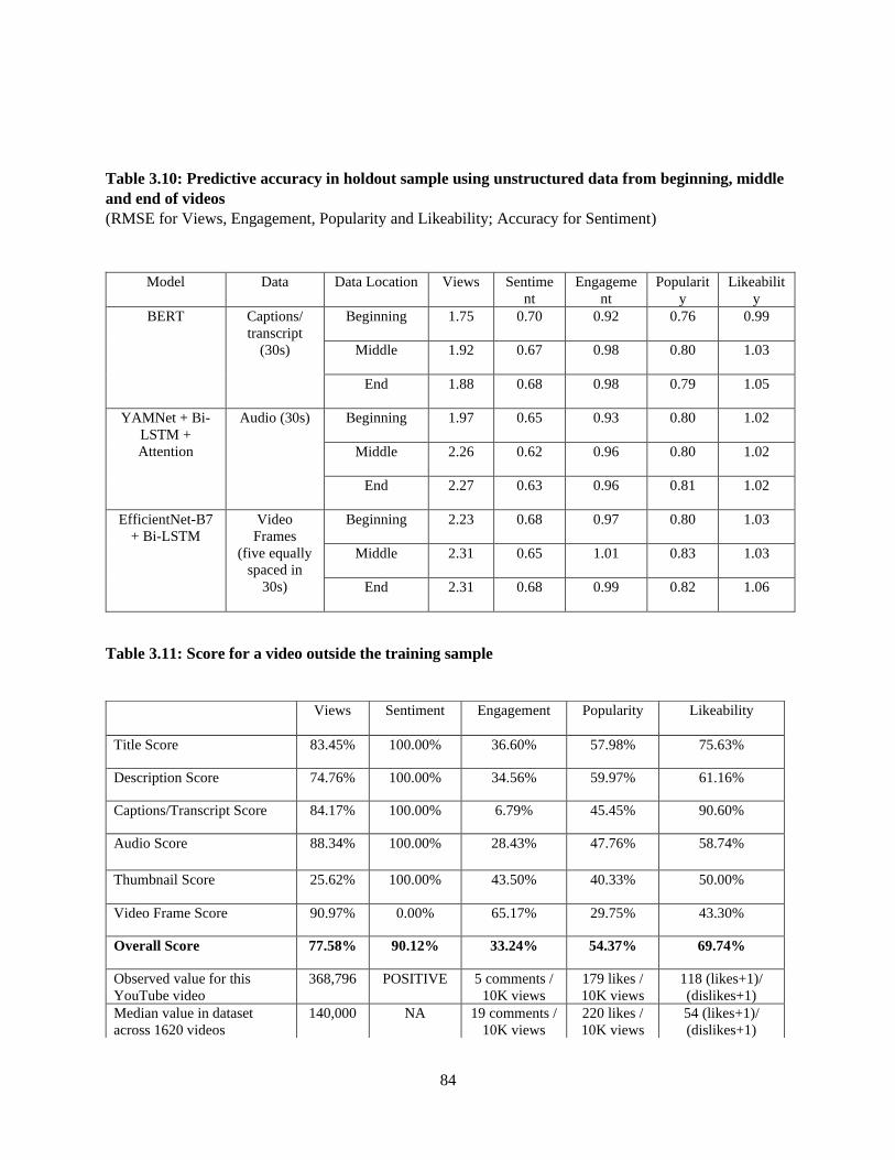
84

Table 3.10: Predictive accuracy in holdout sample using unstructured data from beginning, middle

and end of videos

(RMSE for Views, Engagement, Popularity and Likeability; Accuracy for Sentiment)

Model Data Data Location Views Sentime

nt

Engageme

nt

Popularit

y

Likeabilit

y

BERT Captions/

transcript

(30s)

Beginning 1.75 0.70 0.92 0.76 0.99

Middle 1.92 0.67 0.98 0.80 1.03

End 1.88 0.68 0.98 0.79 1.05

YAMNet + Bi-

LSTM +

Attention

Audio (30s) Beginning 1.97 0.65 0.93 0.80 1.02

Middle 2.26 0.62 0.96 0.80 1.02

End 2.27 0.63 0.96 0.81 1.02

EfficientNet-B7

+ Bi-LSTM

Video

Frames

(five equally

spaced in

30s)

Beginning 2.23 0.68 0.97 0.80 1.03

Middle 2.31 0.65 1.01 0.83 1.03

End 2.31 0.68 0.99 0.82 1.06

Table 3.11: Score for a video outside the training sample

Views Sentiment Engagement Popularity Likeability

Title Score 83.45% 100.00% 36.60% 57.98% 75.63%

Description Score 74.76% 100.00% 34.56% 59.97% 61.16%

Captions/Transcript Score 84.17% 100.00% 6.79% 45.45% 90.60%

Audio Score 88.34% 100.00% 28.43% 47.76% 58.74%

Thumbnail Score 25.62% 100.00% 43.50% 40.33% 50.00%

Video Frame Score 90.97% 0.00% 65.17% 29.75% 43.30%

Overall Score 77.58% 90.12% 33.24% 54.37% 69.74%

Observed value for this

YouTube video

368,796 POSITIVE 5 comments /

10K views

179 likes /

10K views

118 (likes+1)/

(dislikes+1)

Median value in dataset

across 1620 videos

140,000 NA 19 comments /

10K views

220 likes /

10K views

54 (likes+1)/

(dislikes+1)

85

Table 3.12: Variance explained by brand mentions

Model Outcome Covariate

Holdout

√𝑆𝑆𝐸 =

√(𝑦 − �̂�)2

or accuracy

Baseline

√𝑆𝑆𝑇 =

√(𝑦 − �̅�)2

or accuracy

Improve-

ment over

baseline

Variance

explained

by branded

content

Ridge

Regression Views

Two indicators for

brand mention in first

and second half of

description (first 160c)

2.2 2.3 2.4% 7.8%

BERT Views Description (first 160c) 1.6 2.3 30.5%

Ridge

Regression Sentiment

Two indicators for

brand mention in first

and second half of

captions/transcript

(first 30s)

58.0% 50.0% 16.0%

39.7%

BERT Sentiment Captions/Transcript

(first 30s) 70.2% 50.0% 40.4%

86

3.9 Figures

Figure 3.1: Distribution of log view count

Figure 3.2a: Distribution of Log Engagement

Figure 3.2b: Distribution of Log Popularity

87

Figures 3.2c: Distribution of Log Likeability

Figure 3.3: Distribution of average sentiment score across Top 25 comments

Figure 3.4a: Distribution of number of brand mentions in text

88

Figure 3.4b: Distribution of number of brand logos in images

Figure 3.5a Traditional Deep Learning Approach

Figure 3.5b: Interpretable Deep Learning Approach

89

Figure 3.6: BERT Model Framework

Figure 3.7: Audio Model

90

Figure 3.8: Image Model (Video Frames)

Figure 3.9: Combined Model

91

Figure 3.10: Interpretation strategy on holdout sample

Figure 3.11: Attention Weights in captions/transcript (first 30s) of a video

Predicted sentiment: Not Positive

Observed sentiment: Not Positive

92

Figure 3.12: Attention weights in an audio clip (first 30s) of a video

Figure 3.13: Gradient heat map (associated with engagement) in frames of a video

Predicted sentiment: Positive

Observed sentiment: Positive

Predicted Engagement: 15 comments per 10K views

Median Engagement: 19 comments per 10K views

0 sec 7.5 15 sec

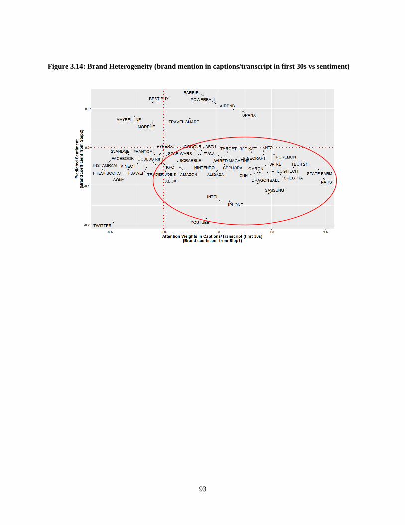
93

Figure 3.14: Brand Heterogeneity (brand mention in captions/transcript in first 30s vs sentiment)

94

CHAPTER IV – Summary & Outlook

Overall, my dissertation adds to the small but growing body of work on modeling viewer behavior on

streaming platforms. It provides solutions and identifies strategies that can improve the welfare of

viewers, platform owners, influencers and brand partners. Specifically, the first essay investigates the

implications of increase in consumer control vis-à-vis content consumption on streaming media. To the

best of my knowledge, this essay is the first attempt at providing a solution for advertising scheduling in

such settings. Specifically, it provides an approach for streaming providers to explore the tradeoff

between content consumption and ad exposure in order to provide a balanced viewing experience. The

recommendations from this approach are available at the granular level of an individual viewer-session.

The approach also uses state-of-the-art methods such as machine learning, but more importantly allows

for causal inference via the use of instrumental variables and provides increased interpretability of the

estimates.

The second essay focuses on an important and growing marketing mechanism, influencer

marketing. This essay investigates how the elements of influencer videos (across text, audio and images)

are related to outcomes that both influencers and marketers care about. Methodologically, the essay

develops a novel deep learning strategy that avoids making a tradeoff between interpretability and

predictive ability. After carrying out predictions using unstructured data, interpretation is carried out ex-

post by quantifying the attention paid on word-pieces in text, moments in audio and items in images while

forming an association with an outcome. This information is used to find significant positive (significant)

relationships between video elements and attention (gradients), followed by the determination of

significant relationships between video elements and the predicted outcome of interest. An added benefit

of this approach is that it allows filtering out relationships that are affected by confounding factors

unassociated with an increase in attention. This significantly reduces the effort required for further causal

work.

Overall, both essays use state-of-the-art machine learning techniques – causal tree-based learning

and interpretable deep learning to answer substantive questions in the domain of ad-supported streaming

media. While the first essay investigates the implications of ad scheduling in streaming environments, the

second essay focuses on the implications of the choice of video features. Together, they provide a

comprehensive perspective on the role of advertising and video design in streaming media. The approach

95

used in both essays can be also applied to other video streaming platforms or platforms where consumers

have control over content consumption, e.g., news media consumption.

Going forward there are some important research questions in this domain that can be

investigated further. First, a comprehensive ad scheduling framework that allows the simultaneous

optimization of different parameters of ad targeting can be developed. Second, it would be important to

examine the evolution of brand usage in influencer videos over time and how this systematically differs

between micro and mega-influencers. Third, understanding how “model” attention correlates with

“visual” or eye-tracking attention in the context of streaming videos can help marketers develop more

cost-effective solutions for their clients. Fourth, understanding the differences between video/ad

characteristics in live-streamed videos and recorded videos can help quantify the advantage or

disadvantage of going live. Last, research that examines the evolving relationship between AI influencers

and viewers could shed light on how consumer needs and desires are going to evolve with the increasing

omnipresence of AI.

96

APPENDICES

APPENDIX A – Appendix to Chapter II

Appendix A.1: Details on Bingeability and Ad Tolerance

I present three more illustrative examples of session viewing behavior and application of the Bingeability

and Ad Tolerance metric. In the first row of each illustration, ‘light gray shaded boxes’ denote Ad Time,

and ‘white shaded boxes’ denote Content Time. In the second row of each illustration, ‘white shaded

dashed line boxes’ denote Session Time, and the ‘black shaded boxes’ (in Example C) indicate the

beginning of the next episode. All values are in minutes.

Example A

Example A shows the behavior of a viewer watching one 23-minute episode of ‘Family Guy’. The

first row shows blocks of time spent watching content (in white) and ads (in light gray). The viewer’s

A

23 min

episode of

Family Guy

13 0.50 6 0.50 2

13 6.5 2.50

Bingeability:

1

No Skipping:

𝐶𝑜𝑛𝑡𝑒𝑛𝑡 𝐿𝑒𝑛𝑔𝑡ℎ𝑖 − 5min ≤ 𝐶𝑜𝑛𝑡𝑒𝑛𝑡 𝑇𝑖𝑚𝑒𝑖

No Excessive Fast-forwarding:

𝐶𝑜𝑛𝑡𝑒𝑛𝑡 𝑇𝑖𝑚𝑒𝑖 ≤ 𝑆𝑒𝑠𝑠𝑖𝑜𝑛 𝑇𝑖𝑚𝑒𝑖−𝐴𝑑 𝑇𝑖𝑚𝑒𝑖

Episode 1: 23 − 5 ≤ 21 Episode 1: 21 ≤ 22 − 1

Ad Tolerance:

− 8 min

∑(𝑃𝑜𝑑𝐷𝑢𝑟𝑎𝑡𝑖𝑜𝑛𝑗 + 𝐶𝑜𝑛𝐸𝑛𝑑𝑗 − (𝐶𝑎𝑙𝑃𝑜𝑑𝑗

𝑛𝑝

𝑗=1

− 𝑃𝑜𝑑𝐷𝑢𝑟𝑎𝑡𝑖𝑜𝑛𝑗−1))

Pod 1: 0.5 + (6 + 2) − (13 − 0) = −4.5

Pod 2: 0.5 + 2 − (6.5 − 0.5) = −3.5

|-----------Block 1-----------|------Block 2 -------|----Block 3-----|

97

viewing experience was interrupted by two ads that were 0.50 minutes long. The first ad was shown after

the viewer viewed 13 minutes of content, and the second ad was shown after the viewer viewed 6

additional minutes of content. After the last ad, the viewer viewed 2 more minutes of content and the

session ended. The second row denotes the calendar time spent corresponding to the blocks of time in the

first row. In Example A, the calendar time spent in each block is equal to the sum of content time and ad

time in the corresponding block. By substituting the values of Example A in equation (2.1), I get,

𝑆𝑒𝑠𝑠𝑖𝑜𝑛 𝑇𝑖𝑚𝑒⏞ 22 minutes

=

𝐶𝑜𝑛𝑡𝑒𝑛𝑡 𝑇𝑖𝑚𝑒⏞ 21 minutes

+ 𝐴𝑑 𝑇𝑖𝑚𝑒⏞ 1 minute

+ 𝐹𝑖𝑙𝑙𝑒𝑟 𝐶𝑜𝑛𝑡𝑒𝑛𝑡 𝑇𝑖𝑚𝑒⏞ 0 minutes

+ 𝑃𝑎𝑢𝑠𝑒𝑠 − 𝐹𝑎𝑠𝑡 𝐹𝑜𝑟𝑤𝑎𝑟𝑑 + 𝑅𝑒𝑤𝑖𝑛𝑑⏞ Unmeasured

As the value of the measured variable on the Left-Hand-Side of the above equation is the same as sum of

the measured variables on the Right-Hand-Side of the equation, the sum of the unmeasured variables is 0

minutes.

Second, both the conditions of the Bingeability metric are satisfied. As I see no evidence of

skipping or excessive fast-forwarding behavior, the value of Bingeability is 1. Third, I discuss the

construction of the Ad Tolerance metric in detail for Example A. I begin by adding the duration of the

first pod which is 0.5 minutes to the amount of content viewed in the remainder of the session (after the

end of the pod), which is 6 + 2 = 8 minutes. I then subtract the calendar time that has elapsed since the

beginning of the session, 𝐶𝑎𝑙𝑃𝑜𝑑𝑗, which is 13 minutes. As there was no pod before this, I have a null

value for 𝑃𝑜𝑑𝐷𝑢𝑟𝑎𝑡𝑖𝑜𝑛𝑗−1. Thus, the total value of the metric for the first pod is −4.5 minutes. Now, I

repeat the same process for the second pod which is also 0.5 minutes in duration. To this I add the content

time viewed in the remainder of the session which is 2 minutes. I then subtract the difference between the

calendar time elapsed since the beginning of the previous pod and the duration of the previous pod, which

is 6.5 − 0.5 = 6. Thus, the total value of the metric for the second pod is −3.5 minutes. On summing up

the values corresponding to each pod, I get a total Ad Tolerance value of −4.5 − 3.5 = −8 minutes. A

negative value of Ad Tolerance suggests that the viewer ended a session after exposure to a commercial

pod which was preceded (at some point) by a long period of no ad exposure. This is true in Example A

where content time between pods (or the period of no ad exposure) was initially large at 13 minutes, and

then reduced to 6 minutes, followed by 2 minutes.

98

Example B

Example B shows the behavior of a viewer watching one 43-minute episode of ‘Chuck’. The

viewer’s viewing experience was interrupted by 6 ads shown in the light gray shaded boxes. The content

time spent in the first block is 3 minutes, but the calendar time is 7 minutes. A higher value of calendar

time suggests that time was spent in pauses or rewinds in this block. This is similarly observed in block 4

and block 7. In block 5, the calendar time spent is 5 minutes, which is less than the sum of ad time and

content time (totaling 6.25 minutes) in the corresponding block. A lower value of calendar time suggests

that time was spent in fast-forwards in this block. By substituting the values of Example B in equation

(2.1), I get,

𝑆𝑒𝑠𝑠𝑖𝑜𝑛 𝑇𝑖𝑚𝑒⏞ 54 minutes

=

𝐶𝑜𝑛𝑡𝑒𝑛𝑡 𝑇𝑖𝑚𝑒⏞ 41 minutes

+ 𝐴𝑑 𝑇𝑖𝑚𝑒⏞ 1.75 minutes

+ 𝐹𝑖𝑙𝑙𝑒𝑟 𝐶𝑜𝑛𝑡𝑒𝑛𝑡 𝑇𝑖𝑚𝑒⏞ 0 minutes

+ 𝑃𝑎𝑢𝑠𝑒𝑠 − 𝐹𝑎𝑠𝑡 𝐹𝑜𝑟𝑤𝑎𝑟𝑑 + 𝑅𝑒𝑤𝑖𝑛𝑑⏞ Unmeasured

On solving the above equation, I find that the sum of the unmeasured variables is 11.25 minutes. This

indicates that more time was spent in pauses or rewinds than in fast-forwards in this session. Second, both

the conditions of the Bingeability metric are satisfied. As I see no evidence of skipping or excessive fast-

forwarding behavior, the value of Bingeability is 1. Third, I adopt a similar process to calculate Ad

Tolerance as done in Example A. It is important to note the use of ‘Caveat 1’ in block 5 of Example B

where there is evidence of fast-forwarding behavior: 𝐶𝑜𝑛𝐸𝑛𝑑𝑗 is chosen as Session Time – Ad Time, 5 −

0.25 = 4.75 minutes, because it is less than Content Time of 6 minutes. I get a total Ad Tolerance value

of 74.25 minutes.

B

43 min

episode of

Chuck

3 0.5 6 0.25 8 0.25 9 0.25 6 0.25 7 0.25 2

7 6.5 8.25 10 5 7.25 10

Bingeability:

1

No Skipping:

𝐶𝑜𝑛𝑡𝑒𝑛𝑡 𝐿𝑒𝑛𝑔𝑡ℎ𝑖 − 5min ≤ 𝐶𝑜𝑛𝑡𝑒𝑛𝑡 𝑇𝑖𝑚𝑒𝑖

No Excessive Fast-forwarding:

𝐶𝑜𝑛𝑡𝑒𝑛𝑡 𝑇𝑖𝑚𝑒𝑖 ≤ 𝑆𝑒𝑠𝑠𝑖𝑜𝑛 𝑇𝑖𝑚𝑒𝑖−𝐴𝑑 𝑇𝑖𝑚𝑒𝑖

Episode 1: 43 − 5 ≤ 41 Episode 1: 41 ≤ 54 − 1.75

Ad Tolerance:

74.25 min

∑(𝑃𝑜𝑑𝐷𝑢𝑟𝑎𝑡𝑖𝑜𝑛𝑗 + 𝐶𝑜𝑛𝐸𝑛𝑑𝑗 − (𝐶𝑎𝑙𝑃𝑜𝑑𝑗

𝑛𝑝

𝑗=1

− 𝑃𝑜𝑑𝐷𝑢𝑟𝑎𝑡𝑖𝑜𝑛𝑗−1))

Pod 1: 0.5 + (6 + 8 + 9 + 4.75 + 7 + 2) − (7 − 0) = 30.25

Pod 2: 0.25 + (8 + 9 + 4.75 + 7 + 2) − (6.5 − 0.5) = 25

Pod 3: 0.25 + (9 + 4.75 + 7 + 2) − (8.25 − 0.25) = 15

Pod 4: 0.25 + (4.75 + 7 + 2) − (10 − 0.25) = 4.25

Pod 5: 0.25 + (7 + 2) − (5 − 0.25) = 4.5

Pod 6: 0.25 + 2 − (7.25 − .25) = −4.75

|-B1-|------Block 2 ----|--------Block 3--------|--------Block 4-----------|--------Block 5-----|---------Block 6-----|----Block 7----|

99

Example C

Example C shows the behavior of a viewer watching two 45-minute episodes of ‘Rescue Me’.

However, the viewer watches only 11.5 minutes of the first episode and 29.5 minutes of the second

episode. There is also evidence of pauses or rewind in block 3 and fast-forwarding in block 4 because

there is mismatch between the calendar time spent and the sum of content time and ad time in those

blocks. It is important to note that evidence of fast-forwarding behavior in block 4 could be for the

content that was rewound in block 3. This is because each block in the illustration does not denote unique

content being viewed due to possible rewinds and fast-forwards by the viewer. By substituting the values

of Example C in equation (2.1), I get,

𝑆𝑒𝑠𝑠𝑖𝑜𝑛 𝑇𝑖𝑚𝑒⏞ 42.3 minutes

=

𝐶𝑜𝑛𝑡𝑒𝑛𝑡 𝑇𝑖𝑚𝑒⏞ 41 minutes

+ 𝐴𝑑 𝑇𝑖𝑚𝑒⏞ 1.30 minutes

+ 𝐹𝑖𝑙𝑙𝑒𝑟 𝐶𝑜𝑛𝑡𝑒𝑛𝑡 𝑇𝑖𝑚𝑒⏞ 0 minutes

+ 𝑃𝑎𝑢𝑠𝑒𝑠 − 𝐹𝑎𝑠𝑡 𝐹𝑜𝑟𝑤𝑎𝑟𝑑 + 𝑅𝑒𝑤𝑖𝑛𝑑⏞ Unmeasured

On solving the above equation, I find that the sum of the unmeasured variables is 0 minutes, but as

mentioned earlier I find definite evidence of fast-forwards, and pauses or rewinds. Second, the first

condition (no skipping) of the Bingeablity metric is not satisfied in both Episode 1 and 2. As none of the

episodes in the session were viewed completely, the value of Bingeability is 0. Third, I adopt a similar

process to calculate Ad Tolerance as done in Example A. I also use ‘Caveat 1’ in block 4 where there is

evidence of fast-forwarding behavior. I get a total Ad Tolerance value of 20.80 minutes.

C

45 min

episode of

Rescue Me

0.30 11.5 7 0.50 20 0.50 2.5

11.80 7 22.5 1

Bingeability:

1

No Skipping:

𝐶𝑜𝑛𝑡𝑒𝑛𝑡 𝐿𝑒𝑛𝑔𝑡ℎ𝑖 − 5min ≤ 𝐶𝑜𝑛𝑡𝑒𝑛𝑡 𝑇𝑖𝑚𝑒𝑖

No Excessive Fast-forwarding:

𝐶𝑜𝑛𝑡𝑒𝑛𝑡 𝑇𝑖𝑚𝑒𝑖 ≤ 𝑆𝑒𝑠𝑠𝑖𝑜𝑛 𝑇𝑖𝑚𝑒𝑖−𝐴𝑑 𝑇𝑖𝑚𝑒𝑖

Episode 1: 45 − 5 ≰ 11.5

Episode 2: 45 − 5 ≰ 29.5

Episode 1: 11.5 ≤ 11.80 − 0.30

Episode 2: 29.5 ≤ 30.5 − 1

Ad Tolerance:

20.80 min

∑(𝑃𝑜𝑑𝐷𝑢𝑟𝑎𝑡𝑖𝑜𝑛𝑗 + 𝐶𝑜𝑛𝐸𝑛𝑑𝑗 − (𝐶𝑎𝑙𝑃𝑜𝑑𝑗

𝑛𝑝

𝑗=1

− 𝑃𝑜𝑑𝐷𝑢𝑟𝑎𝑡𝑖𝑜𝑛𝑗−1))

Pod 1: 0.30 + (11.5 + 7 + 20 + 0.5) − (0 − 0) =

39.30

Pod 2: 0.50 + (20 + 0.50) − (18.80 − 0.30) = 2.5

Pod 3: 0.50 + 0.50 − (22.50 − 0.50) = −21

|-----------Block 1-------------| |--Block 2--|--------------------Block 3-------------------|-----Block 4-----|

100

Appendix A.2: Hulu Data Collection Methodology

In the raw data, a ‘playback ping’ from the Hulu server records the amount of content viewed since the

previous ‘playback ping.’ Similarly, the ‘revenue ping’ records the amount of ad viewed since the

previous ‘revenue ping.’ ‘Playback ping’ and ‘revenue ping’ occur at periodic brief intervals and need not

be in chronological order with respect to the other. For example, a ‘playback ping’ could fall in between

successive ‘revenue pings.’ As content cannot be viewed in between an ad, I record the content viewed

till this ‘playback ping’ as occurring before the commencement of that respective block of ‘revenue

pings.’ In situations when the ‘playback ping’ occurs after the last ‘revenue ping’ (in a block of

consecutive revenue pings), I carry out the following data manipulation: “Calculate the calendar time and

content time captured between these two pings, and then take the difference between the two. If the

difference is negative, I add the absolute value of the difference to the amount of content viewed before

the commencement of the ad.” Thus, for these brief instances (where the difference is negative) right after

the end of an ad, I assume no presence of fast-forwarding behavior because it is less likely. In addition, on

6.7% of the occasions, the amount of ad (pod) watched is registered as greater than the ad (pod) length

due to potential errors in the recording of data by the streaming provider. In these cases, I increase the ad

(pod) length to match the ad (pod) watched.

101

Appendix A.3: Using Different Weights in the Ad Tolerance Metric

As mentioned in subsection “Metric Development”, I had set each of the weights of the three components

of the Ad Tolerance metric to 1. I test a few different scenarios using other combinations of weights and

analyze their effect on the optimized frequency of ad exposure. This is shown in Table A3. The first

scenario assumes that viewers weigh the time spent watching a pod twice as much as the other two

components of the metric. The second scenario assumes that viewers weigh the time spent watching

content after the end of a pod, half as much as the other two components. The third scenario assumes that

viewers weigh the difference between the calendar time elapsed since the beginning of the previous pod

and the duration of the previous pod, twice as much as the other two components of the metric. For each

scenario, I calculate new values of the Ad Tolerance metric, and update the past predictors in Table 2.6d

that correspond to functions for Ad Tolerance Sum, Positive Ad Tolerance Indicator and Ad Tolerance

Session Count. Next, I run the first-stage and second-stage of the model, follow the steps of the Ad

Decision Tree and then run the optimization procedure. The recommended spacing for the set of

observations in each scenario is compared with the recommend spacing for the corresponding set of

observations in the original scenario that had all weights set to 1. The mean absolute difference (MAD)

for these comparisons are also shown in Table A1. The low value of MAD (≤ 1 minute) indicates that my

optimization process is robust to the choice of values of the weights (in the range considered).

Table A1: Different weight combinations of the components of the Ad Tolerance Metric

(MAD (min) on comparing recommended spacing in each scenario with the original recommended spacing)

Scenario Description 𝒘𝟏 𝒘𝟐 𝒘𝟑 MAD

(minutes)

Holdout 1

MAD

(minutes)

Holdout 2

1 𝑷𝒐𝒅𝑫𝒖𝒓𝒂𝒕𝒊𝒐𝒏𝒋 is weighed 2 times the

other components

2 1 1 0.88 0.73

2 𝑪𝒐𝒏𝑬𝒏𝒅𝒋 is weighed 0.5 times the other

components

2 1 2 0.96 0.89

3 𝑪𝒂𝒍𝑷𝒐𝒅𝒋 − 𝑷𝒐𝒅𝑫𝒖𝒓𝒂𝒕𝒊𝒐𝒏𝒋−𝟏 is

weighed 2 times the other components

1 1 2 1.00 0.91

102

Appendix A.4: Metric Validity

A.4.1 Bingeability

I apply both the Episode Count metric and the Bingeability metric to my sample and examine the cases of

mismatch between them in Table A2. Bingeability is different from Episode Count for 45.4% of the

sessions, 89.8% of viewers, 96.2% of TV shows and 94.4% of genres. While the mismatch seems to be

frequent, it is mainly a consequence of skipping behavior and not excessive fast-forwarding behavior.

Skipping behavior is 26 times more likely than excessive fast-forwarding behavior across all sessions.

Table A2: Evidence of Skipping and Excessive Fast-Forwarding

N

(Total count)

Skipping (𝑆) Excessive

Fast-Forwarding

(𝐹𝐹)

Both

(𝑆 ∩ 𝐹𝐹)

Total

(𝑆 ∪ 𝐹𝐹)

Sessions 110,500 45.0% 1.7% 1.3% 45.4%

Viewers 6,157 89.7% 13.6% 13.4% 89.8%

TV shows 558 96.2% 46.0% 46.0% 96.2%

Genre 18 94.4% 88.8% 88.8% 94.4%

I show the relationship between the 0.05th and 99.5th percentile range of Bingeability and Episode Count

in Figure A1. The darker the color of the square, more are the number of points located there. For

example, when Episode Count is 7, there are more instances when Bingeability is 7 than 1.

Figure A1: Bingeability versus Episode Count

(0.5th to 99.5th percentile of Bingeability)

103

|--B1-|-----------------------Block 2 -----------------------------------------|

|-------------------Block 1---------------------------------|-----Block 2-----|

|-B 1--|----Block 2----|----Block 3-----|--------------Block 4-------------|

Now, I compare the trend in viewership of episodes across all 558 TV shows on a weekly (and

monthly) basis using both Episode Count and Bingeability. Trends for both the metrics are compared to

check whether they are both increasing, decreasing or constant. I find that the weekly (and monthly)

trends in viewership popularity are mismatched 21.1% (and 14.7%) of the time across 72.8% (and 26.3%)

of TV shows viewed in my sample. This tells me that inferences about the trend in viewership can change

based on the metric one decides to use. By counting episodes which are not completely watched, Episode

Count typically overstates the popularity of a TV show. Bingeability quantifies the immersive experience

and presents a more conservative estimate of the popularity level. The Bingeability metric by itself can be

useful to various streaming platforms, production studios, advertisers and data measurement companies

who would like to measure the trend in popularity of TV shows streamed on platforms.

A.4.2 Ad Tolerance

I check whether the Ad Tolerance metric can capture differences in behavioral consumption

patterns. For illustration, consider six sessions of six different viewers in Table A3 where each session is

spent viewing 15 minutes of content in addition to ad exposure that is assumed to be randomly delivered.

For ease of exposition, I assume there are no instances of fast-forwards, rewinds or pauses in each

session.

Table A3: Examples of viewing behavior in a session

Session Illustration

Ad

Tolerance

(min)

Ad

Exposure

(min)

Number

of Pods

Viewer 1

2.5 0.50 12.5 10.5 0.50 1

Viewer 2

7.5 0.50 7.5 0.5 0.50 1

Viewer 3

12.5 0.50 2.5 -9.5 0.50 1

Viewer 4

2.5 0.50 2.5 0.50 2.5 0.50 7.5 26.5 1.50 3

|-----------Block 1------------|--------------Block 2 ----------------------|

104

Viewer 5

3.75 0.50 3.75 0.50 3.75 0.50 3.75

12.75 1.50 3

Viewer 6

7.5 0.50 2.5 0.50 2.5 0.50 2.5

4 1.50 3

Viewer 1 is exposed to an ad of length 0.5 minutes after viewing 2.5 minutes of content. After the end of

the ad, the viewer views 12.5 more minutes of content and the session ends. Viewer 2 is exposed to an ad

in the middle of her session while Viewer 3 is exposed to an ad after viewing 12.5 minutes of content.

Across the first three sessions, I observe that Viewer 3 had the most time (12.5 min) to adapt to the

absence of ads and viewed the least amount of content (2.5 min) after the final ad. Hence, Viewer 3 can

be expected to have the lowest Ad Tolerance. Similarly, across the first three sessions, Viewer 1 had the

least time (2.5 min) to adapt to the absence of ads and viewed the most content (12.5 min) after it, and

hence can be expected to have the highest Ad Tolerance.

In the last three sessions, Viewer 4 is exposed to 3 ads in small intervals in the first half of her

session, Viewer 5 is exposed to 3 ads at equally spaced intervals and Viewer 6 is exposed to 3 ads in

small intervals in the second half of the session. Across all the six sessions, I observe that Viewer 3 had

the most time (12.5 min) to adapt to the absence of ads and was exposed to only one ad in total. Hence,

Viewer 3 can be expected to have the lowest Ad Tolerance overall. While both Viewer 1 and Viewer 4

had the least amount of time (2.5 min) to adapt until the first ad, Viewer 4 was exposed to two additional

ads and still ended up watching 15 minutes of content in total. Hence Viewer 4 can be expected to be

have the highest Ad Tolerance. Overall, I can observe that if ads are bunched together in the beginning of

a session, Ad Tolerance is the highest, whereas if the session ends shortly after viewing an ad which was

preceded by a long period of no ad exposure, then the Ad Tolerance is the lowest.

I can compare the Ad Tolerance metric for the six sessions with the simple measures of ‘minutes of

ad exposure’ and ‘number of pods’ in Table A4. I observe that the simple measures are unable to

distinguish between the first three cases or between the last three cases, whereas the Ad Tolerance metric

gives me a unique value for each of the six cases. Thus, I showed that Ad Tolerance is able to capture

differences in behavioral consumption patterns (assuming randomness in ad delivery) in an intuitive

manner, thereby lending further validity to the construction of the metric. Non-randomness in ad delivery

|---B 1---|-------Block 2------|-------Block 3-------|-------Block 4------|

|-------Block 1--------|----Block 2-----|----Block 3-----|-----Block 4----|

105

is controlled with the help of instrumental variables in my model, which is detailed in the subsection

“Model”.

Lastly, using my dataset, I conduct a principal component analysis (with varimax rotation) on the

two metrics and the ‘number of pods’, ‘minutes of ad exposure’ and ‘minutes of content viewed’. I

choose three factors and present their loadings for each variable in Table A4. I find that the factor

loadings for ‘number of pods’, ‘minutes of ad exposure’ and ‘minutes of content viewed’ are very similar

and are dominated by the first factor. On the other hand, Bingeability and Ad Tolerance are dominated by

the third and second factor respectively. This analysis further demonstrates that the two metrics are

capturing different latent constructs.

Table A4: Factor Loadings from a Principal Component Analysis

Factor 1 Factor 2 Factor 3

Bingeability 0.44 0.30 0.85

Ad Tolerance 0.41 0.87 0.29

Number of pods shown 0.82 0.37 0.38

Minutes of ad exposure 0.81 0.40 0.38

Minutes of content viewed 0.76 0.40 0.43

106

Appendix A.5: Modelling Correlation Between Outcomes

I model correlation between the two outcomes—Bingeability and Ad Tolerance—using the regressor

chain approach (Melki et al., 2017). It involves incorporating the predicted value of an outcome as a

covariate to predict another outcome which results in the formation of a chain. This can be formalized by

modifying equation (2.7) in subsection “Model” as follows:

𝑌1𝑡 = 𝑓2(�̂�2𝑡, �̂�1𝑡, �̂�2𝑡 , �̂�3𝑡, �̂�4𝑡,𝑊1𝑡 ,𝑊2𝑡) + 𝑢𝑡

𝑌2𝑡 = 𝑓2(�̂�1𝑡, �̂�1𝑡, �̂�2𝑡 , �̂�3𝑡, �̂�4𝑡,𝑊1𝑡 ,𝑊2𝑡) + 𝑢𝑡

where �̂�1𝑡 and �̂�2𝑡 are the predictions from the original model that are added as covariates to predict 𝑌2𝑡

and 𝑌1𝑡 respectively. Such an approach allows me to capture the correlational influence of one outcome

on the other. The final predictions of the outcomes from the regressor chain approach are then used as

inputs to the Ad Decision Tree, which is followed by running the optimization procedure. Subsequently I

construct a corresponding Decision Support System whose results are shown in Figures A2.1, A2.2 and

A2.3 which are analogous to Figures 2.9a, 2.9b and 2.9c.

The graphs show that for future sessions of current viewers (Holdout 1), the platform and its

viewers are better-off if the platform uses a threshold of 0 to show ads. This results in a 47.5% increase in

ad exposure as compared to observed ad exposure and a 7.19% increase in Bingeability as compared to

initial predicted Bingeability (or a 9.77% increase in Bingeability as compared to observed Bingeability).

Similarly, for new viewers (Holdout 2), the platform and its viewers are better-off if the platform uses a

threshold of 0 to show ads. This results in a 51.0% increase in ad exposure as compared to observed ad

exposure and a 0.93% increase in Bingeability as compared to initial predicted Bingeability (or a 1.14%

decrease in Bingeability as compared to observed Bingeability). This indicates that by capturing

correlation between outcomes for new viewers for whom viewer fixed effects are not known, a best

threshold of 0 to show ads can be achieved. In addition, the presence of an increase of 0.93% in

comparison with initial predicted Bingeability but a decrease of 1.14% in comparison with observed

Bingeability suggests that there are unobserved covariates that influence observed Bingeability, whose

effect cannot be completely captured by modelling correlation between outcomes.

107

Figure A2.1: Percentage change in

optimized ad exposure (�̃�) as compared to

observed ad exposure (𝒏)

Figure A2.2: Percentage change in

optimized Bingeability (�̃�) for Holdout 1

Figure A2.3: Percentage change in

optimized Bingeability (�̃�) for Holdout 2

108

Appendix A.6: Tree Based Methods And Simulated Data

A6.1 Boosting and Random Forests

Boosting or Boosted Regression Trees refer to a weighted linear combination of regression trees, with

each tree trained greedily in sequence to improve the final output (J. Friedman, 2002). This output can be

presented as follows:

𝐹𝑁(𝑥) = ∑𝛼𝑘𝑓𝑘(𝑥)

𝑁

𝑘=1

where, 𝑓𝑘(𝑥) is the function modelled by the 𝑘𝑡ℎ regression tree, and 𝛼𝑘 is the weight associated with it.

The value of 𝑓𝑘 and 𝛼𝑘 are learnt during model training. I adopt a recent extension of gradient boosting

called Extreme Gradient Boosting (XGBoost) because it is a powerful method for making predictions

with structured data (Chen & Guestrin, 2016). For the set of points (𝑥𝑖, 𝑦𝑖), and a loss function

𝑙(𝑦𝑖 , 𝑦�̂�), the XGBoost model minimizes an objective function ℒ to find the step-wise value of 𝑓𝑘(𝑥). For

my application, the loss function 𝑙(𝑦𝑖 , 𝑦�̂�) is the least squares error when the outcome is Ad Tolerance

which is continuous, and negative log likelihood when the outcome is Bingeability which is a count. The

objective function ℒ can be represented as follows:

ℒ = Σ𝑖𝑙(𝑦𝑖 , 𝑦�̂�) + Σ𝑘Ω(𝑓𝑘)

where Ω is the regularization parameter that penalizes the complexity of the model (see Chen and

Guestrin (2016) for details on the objective function). If I set the regularization parameter to 0, I would

get the traditional gradient boosting model. At each step, Newton’s method computes the new value of 𝑓𝑘

that minimizes the average value of the objective function. The step-wise iterations can be shown as

follows:

𝐹𝑘(𝑥) = 𝐹𝑘−1(𝑥) − 𝜂(𝐻𝑘)−1 . 𝑔𝑘

where 𝜂 is the learning rate, 𝑔𝑘 with components 𝑔𝑖𝑘 = [𝑑ℒ(𝑦𝑖,𝐹(𝑥𝑖))

𝑑𝐹(𝑥𝑖) ]𝐹(𝑥𝑖)=𝐹𝑘−1(𝑥𝑖)

is the gradient of the

objective function and 𝐻𝑘 is the second order gradient of the objective function. XGBoost has a faster

computation time than conventional gradient boosting because it employs parallel processing using all the

cores of the computer.

Random Forests refer to the average of thousands of distinct regression trees (Breiman, 2001).

Unlike gradient boosting which uses weak learners or shallow trees at each step, Random Forests average

109

multiple deep trees. Each regression tree is different because it is constructed on a different training

sample by sub-sampling on both observations and covariates. The output of Random Forests can be

represented as follows:

𝐹𝑎𝑣𝑔(𝑥) =1

𝑁∑𝑓𝑘(𝑥)

𝑁

𝑘=1

where, 𝑓𝑘(𝑥) is the function modelled by the 𝑘𝑡ℎ regression tree, which is learnt during model training.

A6.2 Simulation

I simulate data to match the distribution of my real data. Using simulated data, I can create the ground

truth, i.e. I know the extent to which the outcome variable is influenced by the observed covariates in the

model. Hence, I can compare performance of different models in terms of their ability to make predictions

that are closest to the ground truth. I adopt an approach similar to Hartford et al. (2017) to create my

simulated data. I let the source of endogeneity be represented by 𝑣~𝑁(1,0.1) and the four instruments be

represented by 𝑧1 ~ 𝑁(1, 0.1), 𝑧2 ~ 𝑁(1, 0.1), 𝑧3 ~ 𝑁(1, 0.1) and 𝑧4 ~ 𝑁(1, 0.1). The spacing rule (𝑠𝑟)

is represented as follows:

𝑠𝑟 ~ max (𝑊1 + 2𝑣 + 13𝑧1 − 17 , 0)

𝑊1 ~ 𝛼1𝑁(9.1 , 1.5) + (1 − 𝛼1)𝑈(0,0)

𝛼1 ~ 𝐵𝑒𝑟𝑛(0.85)

The correlation between 𝑠𝑟 and 𝑧1 is 0.34 which is close to the correlation of 0.35 in the real data. The

median value of the simulated and real distribution of 𝑠𝑟 is the same at 6.6 min. The length rule (𝑙𝑟) is

represented as follows:

𝑙𝑟 ~ 𝑊2 −𝑣

4+𝑧24

𝑊2 ~ 𝛾2𝑁(0.38, 0.01) + (1 − 𝛾2)(𝛼2𝑁(0.25, 0.002) + (1 − 𝛼2)𝑁(0.5, 0.002))

𝛼2 ~ 𝐵𝑒𝑟𝑛(0.4)

𝛾2 ~ 𝐵𝑒𝑟𝑛(0.2)

110

The correlation between 𝑙𝑟 and 𝑧2 is 0.22 which is close to the correlation of 0.25 in the real data. The

median value of the simulated and real distribution of 𝑙𝑟 is the same at 0.42 min. The diversity rule (𝑑𝑟) is

represented as follows:

𝑑𝑟 ~ 𝑊3 − 𝑣 + 𝑧3

𝑊3~ 𝛼3𝑈(0.15, 1) + (1 − 𝛼3)𝑈(1,1)

𝛼3 ~ 𝐵𝑒𝑟𝑛(0.5)

𝑑𝑟 = {0.05, 𝑑𝑟 ≤ 0.051, 𝑑𝑟 ≥ 1

The correlation between 𝑠𝑟 and 𝑧3 is 0.25 which is close to the correlation of 0.27 in the real data. The

median value of the simulated and real distribution of 𝑑𝑟 is 0.86 and 0.87 respectively. The clumpiness

rule (𝑐𝑟) is represented as follows:

𝑐𝑟 ~ 𝑊4 − 1.1𝑣 + 1.3𝑧4

𝑊4~ 𝛾4(𝛼4𝑁(0.05, 0.02) + (1 − 𝛼4)𝑈(0.3,0.99)) + (1 − 𝛾4)𝑈(1,1)

𝛼4 ~ 𝐵𝑒𝑟𝑛(0.9)

𝛾4 ~ 𝐵𝑒𝑟𝑛(0.8)

𝑐𝑟 = {0, 𝑑𝑟 ≤ 01, 𝑑𝑟 ≥ 1

The correlation between 𝑐𝑟 and 𝑧4 is 0.29 which is close to the correlation of 0.33 in the real data. The

median value of the simulated and real distribution of 𝑐𝑟 is 0.33 and 0.30 respectively.

The outcome variable Bingeability (𝑦1) is simulated to have a complex non-linear relationship with the

covariates. It is represented as follows:

𝑦1~𝑃𝑜𝑖𝑠𝑠𝑜𝑛(𝜆)

𝜆 = max (𝛼𝑖𝑡50+ 0.2𝑠𝑟𝑡 − 0.8𝑙𝑟𝑡 − 1.5𝑑𝑟𝑡 + 0.5𝑊1𝑡

𝑊2𝑡 − 2𝑊2𝑡2 + 𝑒𝑥𝑝(𝑊3𝑡) −𝑊4𝑡 − 0.2 + 𝑢𝑡 , 0)

𝑢 ~ 𝑁(𝜌𝑣, 1 − 𝜌2)

111

𝑢 is the error term that is correlated with 𝑠𝑟, 𝑙𝑟, 𝑑𝑟 and 𝑐𝑟; and 𝜌 is the level of endogeneity which I set at

0.9. 𝑊1,𝑊2, 𝑊3 and 𝑊4 are exogenous covariates which were defined earlier in the equation of each ad

targeting rule. 𝛼𝑖 corresponds to viewer fixed effects and I simulate 500 viewer fixed effects as follows:

𝛼𝑖 = 𝑁(𝑖

10, 0.01) , 𝑖 = {1,… , 500}

I ensure that the sign of the correlation between the outcome variable and the four endogenous variables

in the simulated data is the same as that in the observed data.

The outcome variable Ad Tolerance (𝑦2) is also simulated to have a complex non-linear relationship with

the covariates. It is represented as follows:

𝑦2 =𝛼𝑖𝑡10− 0.05(𝑠𝑟 − 0.9)2 + 4000(𝑙𝑟 − 0.4)2 + 300𝑒−4(𝑑𝑟+0.5)

2− 25 +

10𝑊1𝑊2 − 20𝑊2

2 + 10exp(𝑊3) − 50𝑊4𝑡 + 𝑢

𝑢 ~ 𝑁(𝜌𝑣, 1 − 𝜌2)

The level of endogeneity 𝜌 is set at 0.9 as before. I again ensure that the sign of the correlation between

the outcome variable and the four endogenous variables in the simulated data is the same as that in the

observed data.

The first stage of the model can be represented as follows:

𝑋1𝑡 = 𝑠𝑟𝑡 = 𝑔1(𝑧1𝑡 , 𝑧2𝑡 , 𝑧3𝑡 , 𝑧4𝑡 ,𝑊1𝑡 ,𝑊2𝑡 ,𝑊3𝑡 ,𝑊4𝑡, 𝛼𝑖𝑡) + 𝑒1𝑡

𝑋2𝑡 = 𝑙𝑟𝑡 = 𝑔2(𝑧1𝑡 , 𝑧2𝑡 , 𝑧3𝑡 , 𝑧4𝑡,𝑊1𝑡 ,𝑊2𝑡 ,𝑊3𝑡 ,𝑊4𝑡 , 𝛼𝑖𝑡) + 𝑒2𝑡

𝑋3𝑡 = 𝑑𝑟𝑡 = 𝑔3(𝑧1𝑡 , 𝑧2𝑡 , 𝑧3𝑡 , 𝑧4𝑡,𝑊1𝑡 ,𝑊2𝑡 ,𝑊3𝑡 ,𝑊4𝑡, 𝛼𝑖𝑡) + 𝑒3𝑡

𝑋4𝑡 = 𝑐𝑟𝑡 = 𝑔4(𝑧1𝑡 , 𝑧2𝑡 , 𝑧3𝑡 , 𝑧4𝑡,𝑊1𝑡 ,𝑊2𝑡 ,𝑊3𝑡 ,𝑊4𝑡, 𝛼𝑖𝑡) + 𝑒4𝑡

where, the subscript 𝑡 denotes a session; 𝑒1𝑡, 𝑒2𝑡, 𝑒3𝑡 , and 𝑒4𝑡 are the error terms which are all equal to 𝑣𝑡

in my simulation. The second stage of the model can be represented as follows:

112

𝑦𝑗𝑡 = 𝑓2(�̂�1𝑡, �̂�2𝑡, �̂�3𝑡 , �̂�4𝑡,𝑊1𝑡,𝑊2𝑡,𝑊3𝑡 ,𝑊4𝑡, 𝛼𝑖𝑡) + 𝑢𝑡

where 𝑦𝑗 is either Bingeability (𝑦1) or Ad Tolerance(𝑦2), and �̂�1𝑡 , �̂�2𝑡, �̂�3𝑡, �̂�4𝑡 are the fitted values from

the first stage. Next, I need to determine the counterfactual function or ground truth against which the

performance of different models can be compared. Let me represent this counterfactual function as ℎ, and

for each outcome variable the counterfactual function can be represented as follows:

ℎ1~𝑃𝑜𝑖𝑠𝑠𝑜𝑛(𝜆ℎ)

𝜆ℎ = max (𝛼𝑖50+ 0.2𝑠𝑟 − 0.8𝑙𝑟 − 1.5𝑑𝑟 + 0.5𝑊1

𝑊2 − 2𝑊22 + exp(𝑊3) −𝑊4, 0)

ℎ2 = 𝛼𝑖10− 0.05(𝑠𝑟 − 0.9)2 + 4000(𝑙𝑟 − 0.4)2 + 300𝑒−4(𝑑𝑟+0.5)

2+

10𝑊1𝑊2 − 20𝑊2

2 + 10exp(𝑊3) − 50𝑊4

Note, I removed the intercept terms and the endogenous error to get the equations of the ground truth ℎ1

and ℎ2. Next, I simulate different sizes of the data, as represented in Table A5.1, and split it into an 80%

training sample and 20% holdout sample. I test the performance of three different models: XGBoost,

Random Forests and Linear Regression (2SLS), in terms of their ability to get close to the ground truth, ℎ.

Note that the same model is applied on both the first and second stage. Model performance on the holdout

sample is compared in terms of the RMSE between �̂�1and ℎ1, and �̂�2 and ℎ2 which is shown in Table A5.

I find that XGBoost performs better than Random Forests and Linear Regression (2SLS) in getting close

to the ground truth for both small and large data sizes. Hence, I use the XGBoost model to analyze my

observed data.

Table A5: Comparison of Model Performance (RMSE) on holdout sample

Bingeability Ad Tolerance

Data Size Linear

Regression

Random

Forests

XGBoost Linear

Regression

Random

Forests

XGBoost

5,000 2.12 1.93 1.90 50.48 34.75 25.97

25,000 1.90 1.88 1.84 48.81 31.74 24.72

50,000 1.89 1.88 1.82 48.04 29.55 24.82

75,000 1.88 1.88 1.82 48.43 28.97 24.61

100,000 1.87 1.87 1.81 48.64 29.50 24.66

113

Appendix A.7: Cross-Validation for XGBoost

The parameters of the XGBoost model for the observed data are set by cross-validation. I carry out 5-fold

cross validation on the training sample by dividing viewers into five different folds. This process is

repeated 10 different times with random splits made on the training data to determine the 5 folds. The

parameters that are tuned are as follows:

• Maximum depth of a tree: {4,6}

• Minimum threshold for loss reduction, 𝛾: {0,5}

• Regularization parameter on weights of a leaf: {0,1}

• Row subsampling fraction: {0.8,1}

• Column subsampling fraction at the node level: {0.8,1}

The minimum number of observations on each node of a leaf is set to 1, and the value of the learning rate

𝜂 is set by judgement to ensure that the cross-validation process does not take unduly long to finish. I

have 25 = 32 distinct parameter combinations and 10 iterations for each parameter combination. As an

exhaustive grid search for a total of 320 iterations over 74,996 observations (in the training sample) will

take unduly long to finish, I use an efficient three step process to decide the final parameter combination

to be used to tune the training sample.

• Step 1: I use a “fractional factorial design” to design 25−2 = 8 combinations of the parameters

that are balanced and orthogonal. Then I run the cross-validation routine 10 times for these 8

combinations for a total of 80 iterations. Then I average the performance measure (e.g. RMSE or

Negative Log Likelihood) across the 10 iterations for each of the 8 combinations and rank the

combinations in order of best to worst performance.

• Step 2: Next, I analyze the performance across the 8 orthogonal combinations and identify other

potential parameter combinations that could result in an improved cross-validation performance. I

run the cross-validation routine 10 times for each of these newly identified parameter

combinations. Then I average the performance measure across the 10 iterations for each of the

newly identified combinations.

• Step 3: The parameter combination that leads to the lowest average value of the performance

measure across the 10 repetitions for the parameter combinations in Step 1 and Step 2 is chosen

to train the model.

114

Appendix A.8: Optimization Procedure

Part 1

My objective function is subject to the constraint of not detracting from the content consumption

experience. This constraint corresponds to the equation of the Ad Tolerance metric, originally shown in

equation (2.4), which is reproduced below.

𝐴𝑑 𝑇𝑜𝑙𝑒𝑟𝑎𝑛𝑐𝑒 =∑(𝑤1𝑃𝑜𝑑𝐷𝑢𝑟𝑎𝑡𝑖𝑜𝑛𝑗 +𝑤2𝐶𝑜𝑛𝑡𝑒𝑛𝑡𝐸𝑛𝑑𝑗 −𝑤3(𝐶𝑎𝑙𝑒𝑛𝑑𝑎𝑟𝑃𝑜𝑑𝑗

𝑛𝑝

𝑗=1

− 𝑃𝑜𝑑𝐷𝑢𝑟𝑎𝑡𝑖𝑜𝑛𝑗−1))

This constraint ensures that the optimization routine (of ad maximization) takes cognizance of the

predicted values of Ad Tolerance and Bingeability, thus preventing the routine from making scheduling

recommendations that can cause a reduction in the amount of content viewed. Now, I substitute the

variables from equation (2.9) in the above equation, i.e. 𝑛𝑝 = 𝑛; 𝑃𝑜𝑑𝐷𝑢𝑟𝑎𝑡𝑖𝑜𝑛𝑗 = 𝑑; 𝐶𝑜𝑛𝑡𝑒𝑛𝑡𝐸𝑛𝑑𝑗 =

�̂�𝑒 − 𝑗𝑠 where 𝑗 is pod number; and 𝑃𝑜𝑑𝐷𝑢𝑟𝑎𝑡𝑖𝑜𝑛𝑗−1 = 𝑑. Hence, I can rewrite the constraint

corresponding to the Ad Tolerance metric as follows:

𝐴𝑑 𝑇𝑜𝑙𝑒𝑟𝑎𝑛𝑐𝑒 =∑(𝑤1𝑑 + 𝑤2(�̂�𝑒 − 𝑗𝑠) − 𝑤3(𝐶𝑎𝑙𝑒𝑛𝑑𝑎𝑟𝑃𝑜𝑑𝑗 − 𝑑))

𝑛

𝑗=1

To substitute values into 𝐶𝑎𝑙𝑒𝑛𝑑𝑎𝑟𝑃𝑜𝑑𝑗, I use equation (2.1) which is reproduced below:

𝑆𝑒𝑠𝑠𝑖𝑜𝑛 𝑇𝑖𝑚𝑒⏞ Measured

= 𝐶𝑜𝑛𝑡𝑒𝑛𝑡 𝑇𝑖𝑚𝑒 + 𝐴𝑑 𝑇𝑖𝑚𝑒 + 𝐹𝑖𝑙𝑙𝑒𝑟 𝐶𝑜𝑛𝑡𝑒𝑛𝑡 𝑇𝑖𝑚𝑒⏞ +

Measured

𝑃𝑎𝑢𝑠𝑒𝑠 − 𝐹𝑎𝑠𝑡 𝐹𝑜𝑟𝑤𝑎𝑟𝑑 + 𝑅𝑒𝑤𝑖𝑛𝑑⏞ Unmeasured

Using the variables in equation (2.9), the above equation can be rewritten as follows:

𝐶𝑎𝑙𝑒𝑛𝑑𝑎𝑟𝑃𝑜𝑑𝑗⏞ Measured

= 𝑠 + 𝑑 + 𝑓𝑗⏞ Measured

+ 𝑢𝑗⏞Unmeasured

where, 𝑓𝑗 is duration of filler content viewed from the beginning of the pod 𝑗-1 till the beginning of pod 𝑗

and 𝑢𝑗 = (𝑝𝑎𝑢𝑠𝑒𝑠 − 𝑓𝑎𝑠𝑡 𝑓𝑜𝑟𝑤𝑎𝑟𝑑 + 𝑟𝑒𝑤𝑖𝑛𝑑)𝑗 is the sum of the unmeasured variables from the

beginning of pod 𝑗-1 till the beginning of pod 𝑗. A viewer is not expected to be immersed in the viewing

experience while watching filler content; hence I allow the viewer to skip it or fast forward it by setting 𝑓𝑗

to 0. As the unmeasured variables—Pauses, Fast Forward and Rewind—are directly under viewer control

115

and cannot be controlled by the streaming provider, I set 𝑢𝑗 to 0. Hence, I can rewrite the constraint

(equation (2.10)) as follows:

�̂� =∑(𝑤1𝑑 + 𝑤2(�̂�𝑒 − 𝑗𝑠) − 𝑤3(𝑠 + 𝑑 − 𝑑))

𝑛

𝑗=1

where the predicted value of Ad Tolerance is shown as �̂�. After summing over the variables, I get

�̂� = 𝑤1𝑛𝑑 + 𝑤2 (𝑛�̂�𝑒 −𝑛(𝑛+1)

2𝑠) − 𝑤3𝑛𝑠

Part 2

The partial derivative of �̃� with respect to �̂� is shown below:

𝜕�̃�

𝜕�̂�=1 + 2�̂� + 3�̂�𝑒 + √Δ

(1 + �̂�𝑒)√Δ > 0

The above equation is always > 0 because �̂� ≥ 1, �̂� > 0, √Δ > 0 and 𝑒 > 0. Thus, controlling for �̂� and

e, an increase in Ad Tolerance results in an increase (decrease) in the number of ads �̃� (spacing

�̃�) (∵ �̃� ∝1

�̃� ). The partial derivative of �̃� with respect to �̂� is shown below:

𝜕�̃�

𝜕�̂�=𝑒(�̂�𝑒 − 3�̂��̂�𝑒 + √Δ(1 − �̂�) + �̂� − 2�̂�2 − 1)

(1 + �̂�𝑒)2√Δ

On substituting the values of �̂�, �̂� and 𝑒 from the observations in Set C (from Table 2.9) into the above

equation, I find that the partial derivative is almost always negative. For the few instances when �̂� ∈

(0, 0.5 min), the value of the partial derivative is positive. Thus, controlling for �̂� and e, an increase in

Bingeability almost always results in a decrease (increase) in the number of ads �̃� (spacing �̃�). The

interpretation of the partial derivative for the few instances when �̂� ∈ (0, 0.5 min) can be understood as

the effect of the algorithm to ensure a minimum level of Ad Tolerance before recommending a decrease

(increase) in the number of ads �̃� (spacing �̃�) for an increase in Bingeability, �̂�.

Overall, the partial derivatives help illustrate the direction of the influence of the metrics on the

recommended spacing �̃�.

116

Appendix A.9: Recommended Schedule Versus A Naïve Heuristic

I develop a naïve heuristic based on viewer response to ad delivery that could be used to recommend ad

spacing. As mentioned in the “Introduction” section, viewer response to ad delivery has been studied in

past work by Schweidel and Moe (2016) who find that ad exposure is negatively correlated with content

consumption. Hence, one naïve heuristic for a session (𝑖) is the ratio of total time spent watching TV

shows in the past week by the viewer (before the commencement of the session) to the total number of

pods shown to that viewer while watching TV shows in the past week. It can be represented as follows:

𝑁𝑎𝑖𝑣𝑒 𝑆𝑝𝑎𝑐𝑖𝑛𝑔𝑖 =𝑇𝑜𝑡𝑎𝑙 𝐶𝑜𝑛𝑡𝑒𝑛𝑡 𝑇𝑖𝑚𝑒𝑖𝑇𝑜𝑡𝑎𝑙 𝑁𝑢𝑚𝑏𝑒𝑟 𝑜𝑓 𝑃𝑜𝑑𝑠𝑖

The heuristic is naive for mainly the following reasons (1) it does not incorporate the frequency (or

spacing) of pod exposure in the viewing experience, as done by the Ad Tolerance metric (2) it does not

account for fast-forwarding or skipping behavior, as done by the Bingeability metric, and (3) it does not

control for the non-randomness in ad delivery, as done in my model using instrumental variables.

A density distribution of the naive spacing for those sessions in Set C (from Table 2.9) is shown in

Figures A3.1a and A3.1b for Holdout 1 and Holdout 2 respectively. I ignore those sessions which are the

first sessions of the viewers, because the value of the naïve spacing metric will result in a ‘divide by 0’

error. The median value of the naive spacing for Holdout 1 (future sessions of the viewers in the training

sample) is 8.30 minutes and its 2.5th to 97.5th percentile range is from 4.19 to 17.96 minutes. The median

value of the naive spacing for Holdout 2 (new viewers) is 9.16 minutes and its 2.5th to 97.5th percentile

range is from 5.01 to 18.11 minutes.

The distribution of the ratio of (optimized) recommended spacing and naïve spacing is shown in

Figures A3.2a and A3.2b. I ignore those sessions where the naïve spacing is 0 minutes to avoid a ‘divide

by 0’ error and also because they suggest showings ads continuously without any show content in

between which is not meaningful. The median value of the ratio is 0.50 in Figure A3.2a and 0.47 in

Figure A3.2b. As the median is a lot less than 1 (which is the 90th percentile in Figure A3.2a and 95th

percentile in Figure A3.2b), I can conclude that the naïve heuristic suggests a lower frequency (longer

spacing) a lot more often than the (optimized) recommendation, thus losing out on opportunities to

maximize ad exposure.

Finding the ratio of the naïve spacing with the average observed spacing reveals that the median of

the distribution is 1.25 for each holdout sample. This demonstrates that on average the naïve schedule

recommends showing ads less frequently (with a longer spacing) as compared to observed practice. I

quantify the decrease in ad exposure by using the naïve heuristic as done in the subsection “Decision

117

Support System” for a Bingeability threshold of 0. Ad exposure increases by −35% for Holdout 1 and by

−40% for Holdout 2 as compared to observed practice. On the other hand, content consumption increases

by 11.56% as compared to initial predicted Bingeability (and by 12.47% compared to observed

Bingeability) for Holdout 1 and by 4.62% compared to initial predicted Bingeability (and 1.44%

compared to observed Bingeability) for Holdout 2. As the naïve heuristic is unable to make both the

platform and the viewers better off, it is inferior to the optimized ad schedule.

Figure A3.2a: Density of the Ratio of Recommended

Spacing and Naïve Spacing in Holdout 1

(2.5th to 97.5th percentile)

Figure A3.1a: Density of Naïve Spacing in

Holdout 1

(2.5th to 97.5th percentile)

Figure A3.1b: Density of Naïve Spacing in

Holdout 2

(2.5th to 97.5th percentile)

95th percentile 90th percentile

Figure A3.2b: Density of the Ratio of

Recommended Spacing and Naïve

Spacing in Holdout 2

(2.5th to 97.5th percentile)

118

APPENDIX B – Appendix to Chapter III

Appendix B.1: BERT Encoders (in Text Model)

BERT Encoders comprise a set of 12 sequentially arranged identical encoders, and I illustrate the

architecture of one encoder in Figure B1. 74 I explain an example with a sentence that has only two tokens,

and this can be extended to any example that has a maximum of 512 tokens, which is the maximum limit

of the pre-trained BERT model. The combined vector of the initial token embedding (𝑥1, 𝑥2) and

positional encoding (𝑡1, 𝑡2) results in the vectors (𝑥1′ , 𝑥2′) that are passed through self-attention heads

which incorporate information of other relevant tokens into the focal tokens. The architecture of the self-

attention head is explained further ahead. The outputs of the self-attention head (𝑧1, 𝑧2) are then added

with the original input (𝑥1′ , 𝑥2′) using a residual connection (shown with a curved arrow) and normalized

(using mean and variance). The outputs (𝑧′1, 𝑧′2) are passed through identical feed forward networks that

have a GELU (Gaussian Error Linear Unit) activation function, i.e. 𝑔𝑒𝑙𝑢(𝑥) = 0.5𝑥 (1 + 𝑒𝑟𝑓 (𝑥

√2 )).

The gelu activation combines the advantages of the ReLU (Rectified Linear Unit) non-linearity (i.e.,

𝑒𝑙𝑢(𝑥) = 𝑚𝑎𝑥(0, 𝑥)) with dropout regularization. The outputs of the feed forward network are added

with the inputs (𝑧′1, 𝑧′2) using a residual connection and normalized again before being fed to the next

encoder in sequence. In addition, each sub-layer is first followed by a dropout probability of 0.1 before

being added and normalized.

74 My figures are inspired from the work of Jay Alammar.(see Alammar (2018) for more details)

119

Figure B1: Encoders

Next, I explain the self-attention heads using the framework shown in Figure B2. There are 12

self-attention heads that capture the contextual information of each token in relation to all other tokens

used in the text. In other words, this allows the model to identify and weigh all other tokens in the text

that are important when learning the vector representation of the focal token. I use this to visualize the

strength of association between the tokens in the text and the outcome of interest in Section 3.5.2.

The inputs (𝑥1′ , 𝑥2′) are concatenated and multiplied with three weight matrices, 𝑊𝑞 ,𝑊𝑘and

𝑊𝑣 (that are fine-tuned during model training) to get three vectors – 𝑄 (Query), 𝐾(Key) and 𝑉(Value).

These three vectors are combined using an attention function (A):

𝐴(𝑄,𝐾, 𝑉) = 𝑧0′′ = 𝑠𝑜𝑓𝑡𝑚𝑎𝑥 (

𝑄.𝐾𝑇

√𝑑𝑘) . 𝑉

where, 𝑑𝑘, the dimension of the Key vector, is chosen to be 64 and is equal to the dimensions of the other

two vectors 𝑑𝑞 and 𝑑𝑣; and 𝑠𝑜𝑓𝑡𝑚𝑎𝑥(𝑥) =𝑒𝑥𝑖

∑ 𝑒𝑥𝑖𝑚𝑖=1

. The division by √𝑑𝑘 is performed to ensure stable

gradients. The computation of 𝑧0′′ is for one attention head, and this is carried out in parallel for 11

additional attention heads to give me 12 vectors, 𝑧0′′…𝑧12

′′ , which are concatenated to produce 𝑧′′. This is

multiplied with a weight vector 𝑊𝑂 (which is fine-tuned during model training) to produce output

(𝑧1, 𝑧2). The use of 11 additional attention heads allows the model to capture more complex contextual

information.

120

Figure B2: Self-Attention Heads

121

Appendix B.2: MobileNet V1 followed by Bi-LSTM with Attention (in Audio Model)

The MobileNet v1 architecture is illustrated in detail in Table B1. Each row describes Stage 𝑖 with input

dimension [�̂�𝑖, �̂�𝑖] (resolution), output channels �̂�𝑖 (width) and �̂�𝑖 layers (depth).

Table B1: MobileNet-v1 architecture

Stage

𝑖

Operator

�̂�𝑖

Resolution

(�̂�𝑖 x �̂�𝑖) (Height x Width)

Width

�̂�𝑖 (Channels)

Depth

�̂�𝑖 (Layers)

Pre-trained

Weights

1 Conv, k3x3, s2 96 x 64 32 1

Yes

2 MConv, k3x3, s1 48 x 32 64 1

3 MConv, k3x3, s2 48 x 32 64 1

4 MConv, k3x3, s1 24 x 16 128 1

5 MConv, k3x3, s2 24 x 16 128 1

6 MConv, k3x3, s1 12 x 8 256 1

7 MConv, k3x3, s2 12 x 8 256 1

8 MConv, k3x3, s1 6 x 4 512 5

9 MConv, k3x3, s2 6 x 4 512 1

10 MConv, k3x3, s2 3 x 2 1024 1

11 Global Average Pooling 3 x 2 1024 1

12 Dense 1 x 1 521 1

Stage 1 has a regular convolution operation, whereas Stage 2 to 10 have the Mobile Convolution which is

the main building block of the architecture. It is represented as “MConv, 𝑘 x 𝑘, s” where 𝑘 x 𝑘 = 3 x 3 is

the size of the kernel and 𝑠 = {1,2} is the stride. MConv divides the regular convolution operation into

two steps – depth wise separable convolutions and point wise convolution, thus increasing the speed of

computation (see Howard et al. (2017) for details). Stage 11 has a Global Average Pooling Layer that

averages the inputs along its height and width and passes its output to Stage 10 which is a Dense output

layer with 521 logistic functions that gives the per class probability score corresponding to the 960 ms

input segment. I use a hop size of 490 ms so that I get an even number of 60 time step predictions

corresponding to the 30 seconds of input. The resulting output vector has a dimension of 521x60 (audio

classes x time steps) for each 30 second clip.

The output from MobileNet v1 is passed as input to the Bi-LSTM with attention mechanism,

shown in Figure B3. I use two layers of LSTM cells – the first layer is a 32 unit Bidirectional LSTM layer

and the second layer is a 64 unit (unidirectional) LSTM layer. They are separated by an attention

mechanism as shown in Figure B3. Each audio segment 𝑥𝑚 <521,1>, where 𝑚 is the total number of

moments (time steps), is passed as input to each cell of the Bidirectional LSTM layer. This layer is made

bidirectional to allow it to capture the interdependence between sequential audio segments from both

directions. The sequential nature of LSTM cells in a layer allow the model to capture dependencies

122

between audio segments that are separated from each other (see the LSTM paper by Gers et al. (1999) for

more details). I adopt the attention mechanism used for neural machine translation by Bahdanau et al.

(2014) to help the Bi-LSTM model focus on more important parts of the input. The mechanism weighs

the output activations (𝑎<𝑡> = [�⃗�<𝑡>, �⃖�<𝑡>], 𝑡 = 1 to 𝑚) from each cell of the pre-attention Bi-LSTM

layer before passing the contextual output, 𝑐<𝑡> , to the post-attention LSTM layer above it. In addition,

each cell of the attention mechanism takes as input the output activation 𝑠(𝑡 − 1) from each preceding

cell of the post-attention LSTM layer which allows it to factor in the cumulative information learnt by the

model till that time step (see Bahdanau et al. (2014) for more details on the attention mechanism). The

output of the last cell in the post-attention LSTM layer is passed to an output layer which has a linear

activation function for the four continuous outcomes and a sigmoid activation function for sentiment. The

context vector 𝑐<𝑚> from the last cell of the attention mechanism allows visualization of the relative

weights placed by the model along the time dimension of the input in order to form an association with

the outcome of interest. Audio moments that have higher weight are more important while forming an

association between the audio clip and the outcome of interest.

Figure B3: Bi-LSTM with Attention

�⃗�<0> = 0ሬ⃗ �⃖�<𝑚+1> = 0ሬ⃗

�⃗�<1> �⃗�<𝑚>

𝑠<0> = 0ሬ⃗ 𝑠<1> 𝑠<𝑚−1>

𝑐<1> 𝑐<𝑚> 𝑐<2>

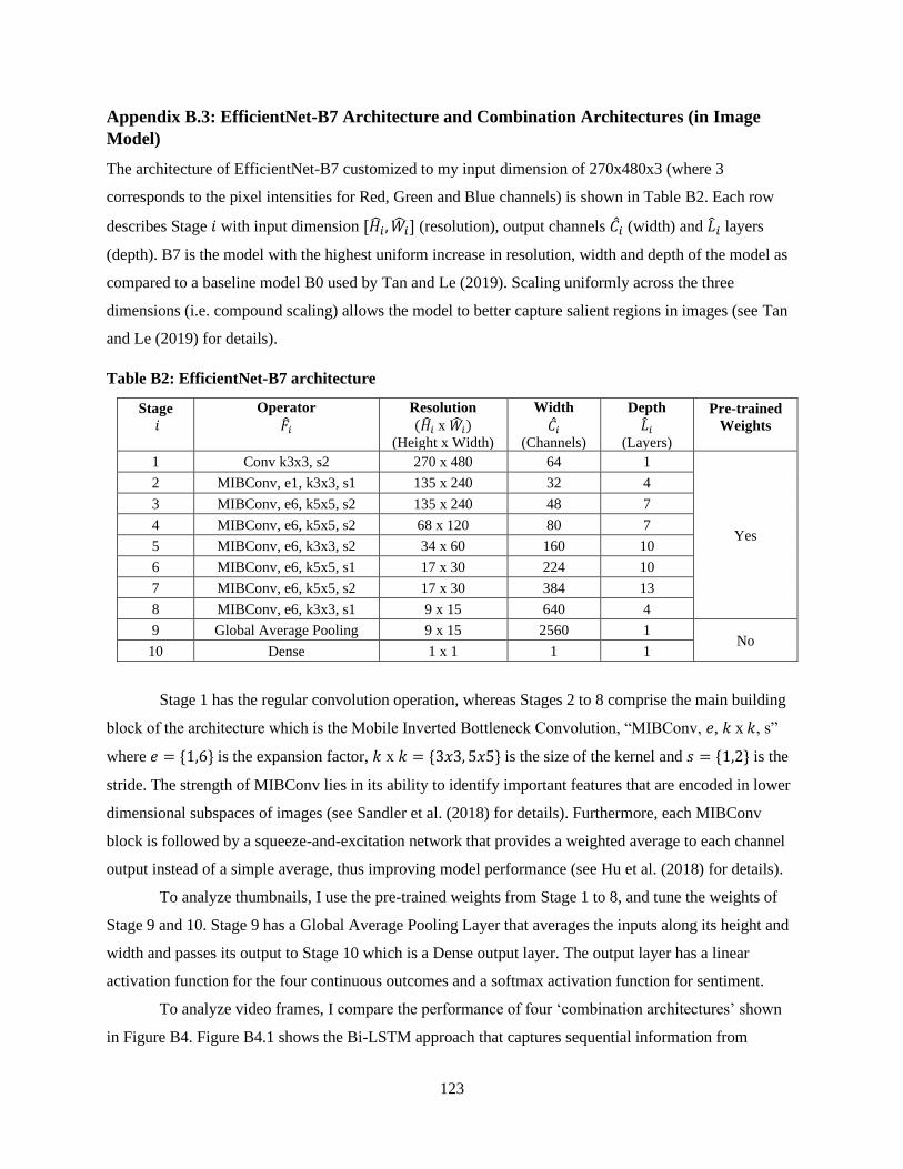
123

Appendix B.3: EfficientNet-B7 Architecture and Combination Architectures (in Image

Model)

The architecture of EfficientNet-B7 customized to my input dimension of 270x480x3 (where 3

corresponds to the pixel intensities for Red, Green and Blue channels) is shown in Table B2. Each row

describes Stage 𝑖 with input dimension [�̂�𝑖, �̂�𝑖] (resolution), output channels �̂�𝑖 (width) and �̂�𝑖 layers

(depth). B7 is the model with the highest uniform increase in resolution, width and depth of the model as

compared to a baseline model B0 used by Tan and Le (2019). Scaling uniformly across the three

dimensions (i.e. compound scaling) allows the model to better capture salient regions in images (see Tan

and Le (2019) for details).

Table B2: EfficientNet-B7 architecture

Stage

𝑖

Operator

�̂�𝑖

Resolution

(�̂�𝑖 x �̂�𝑖) (Height x Width)

Width

�̂�𝑖 (Channels)

Depth

�̂�𝑖 (Layers)

Pre-trained

Weights

1 Conv k3x3, s2 270 x 480 64 1

Yes

2 MIBConv, e1, k3x3, s1 135 x 240 32 4

3 MIBConv, e6, k5x5, s2 135 x 240 48 7

4 MIBConv, e6, k5x5, s2 68 x 120 80 7

5 MIBConv, e6, k3x3, s2 34 x 60 160 10

6 MIBConv, e6, k5x5, s1 17 x 30 224 10

7 MIBConv, e6, k5x5, s2 17 x 30 384 13

8 MIBConv, e6, k3x3, s1 9 x 15 640 4

9 Global Average Pooling 9 x 15 2560 1 No

10 Dense 1 x 1 1 1

Stage 1 has the regular convolution operation, whereas Stages 2 to 8 comprise the main building

block of the architecture which is the Mobile Inverted Bottleneck Convolution, “MIBConv, 𝑒, 𝑘 x 𝑘, s”

where 𝑒 = {1,6} is the expansion factor, 𝑘 x 𝑘 = {3𝑥3, 5𝑥5} is the size of the kernel and 𝑠 = {1,2} is the

stride. The strength of MIBConv lies in its ability to identify important features that are encoded in lower

dimensional subspaces of images (see Sandler et al. (2018) for details). Furthermore, each MIBConv

block is followed by a squeeze-and-excitation network that provides a weighted average to each channel

output instead of a simple average, thus improving model performance (see Hu et al. (2018) for details).

To analyze thumbnails, I use the pre-trained weights from Stage 1 to 8, and tune the weights of

Stage 9 and 10. Stage 9 has a Global Average Pooling Layer that averages the inputs along its height and

width and passes its output to Stage 10 which is a Dense output layer. The output layer has a linear

activation function for the four continuous outcomes and a softmax activation function for sentiment.

To analyze video frames, I compare the performance of four ‘combination architectures’ shown

in Figure B4. Figure B4.1 shows the Bi-LSTM approach that captures sequential information from

124

different video frames. Each EfficientNet-B7 model takes a different video frame as input and provides

the output from Stage 8 to the Global Average Pooling (GAP) Layer. This is followed by Dense Middle

Layers (that use ReLU activation for continuous outcomes and sigmoid activation for the binary

outcome), which is followed by a single Bi-LSTM layer with 256 memory cells, and finally a Dense

output layer (that uses linear activation for continuous outcomes and softmax activation for the binary

outcome). Figures B4.2, B4.3 and B4.4 show three approaches that preserve the spatial information across

different video frames. The Max-GAP approach finds the maximum value across the [9x15x2560] Stage

8 output from each EfficientNet-B7 model, which is followed by a GAP layer that reduces the dimensions

to [1x1x2560]. The GAP-Max approach first finds the global average across each Stage 8 output, which is

then followed by the Max operation, while the C-GAP approach concatenates the GAP outputs. Across all

four approaches, I use the pre-trained weights from Stage 1 to 8 for each EfficientNet-B7 model and tune

the weights of the final layers.

Figure B4.1: Bi-LSTM Figure B4.2: Max-GAP

125

Figure B4.3: GAP-Max Figure B4.4: C-GAP

126

Appendix B.4: Comparison of Model Performance with Benchmarks

I first compare the predictive performance from the BERT Text Model with four benchmarks in Table

B3.1. The benchmark models include an LSTM (with a 300 dimensional Glove word vector embedding),

CNN model (X. Liu et al., 2019), CNN-LSTM (Chakraborty et al., 2019) and CNN-Bi-LSTM.

Table B3.1: Comparison of Text Model performance in holdout sample

(RMSE for Views; Accuracy for Sentiment)

Outcome Covariate LSTM CNN CNN-

LSTM

CNN-Bi-

LSTM

BERT

Views Title 2.11 1.73 1.75 1.68 1.66

Description (first 160c) 2.27 1.69 1.68 1.67 1.57

Captions/transcript (first 30s) 2.28 1.82 1.80 1.76 1.75

Sentiment Title 0.67 0.70 0.70 0.70 0.72

Description (first 160c) 0.50 0.69 0.69 0.69 0.69

Captions/transcript (first 30s) 0.67 0.70 0.70 0.70 0.70

As can be seen in Table B3.1, BERT has the best performance for both views (lowest RMSE) and

sentiment (highest accuracy), with a maximum performance improvement of 6% for ‘views-description’

as compared to CNN Bi-LSTM.

I then compare the model performance of the Audio model as per the benchmarks discussed in

Section 3.4.2 and present the results in Table B3.2. I find that the addition of MobileNet v1 (Model 2)

helps improve accuracy when predicting sentiment, but there is no performance improvement when

predicting views. Addition of the attention mechanism (Model 3) results in an improvement in both

RMSE (by 10%) when predicting views and accuracy (by 1.5%) when predicting sentiment, thus

demonstrating the benefit of capturing relative attention weights in the model.

Table B3.2: Comparison of Audio Model performance in holdout sample

(RMSE for Views; Accuracy for Sentiment)

Outcome Model 1:

Mel Spectrogram +

Bi-LSTM

Model 2:

Mel Spectrogram +

MobileNet v1 +

Bi-LSTM

Model 3:

Mel Spectrogram +

MobileNet v1 +

Bi-LSTM +

Attention

Views 2.19 2.19 1.97

Sentiment 0.59 0.64 0.65

127

Next, I compare the performance of the (pre-trained) EfficientNet-B7 with a 4-layer CNN model

using thumbnails in Table B3.3. I see a substantial improvement in both RMSE (by 41%) and accuracy

(by 26%) when using EfficientNet-B7, thus demonstrating the benefits of both deeper

architecture and transfer learning with image data.75

Table B3.3: Comparison of Thumbnail Model performance in holdout sample

(RMSE for Views; Accuracy for Sentiment)

Next, I compare the performance of the four Video Frame Models in Table B3.4 using two

frames in each video clip – 0 sec and 30 sec.

Table B3.4: Comparison of Video Frame Model (0s,30s) performance in holdout sample

(RMSE for Views; Accuracy for Sentiment)

Outcome Bi-LSTM Max-GAP GAP-Max C-GAP

Views 2.28 3.16 2.88 5.53

Sentiment 0.66 0.66 0.66 0.66

I find that the Bi-directional LSTM architecture which captures the sequential information from

two video frames performs better than the other three models that capture only spatial information while

predicting views. However, all four models perform equally well in predicting sentiment. This

demonstrates that capturing sequential information is more important for predicting views but not as

important for predicting sentiment. As the Bi-LSTM model is the best overall, I use it to predict all the

outcomes. Furthermore, I demonstrate sequential improvement in predictive performance when I add

additional video frames to the model by reducing the time interval by half at each step, in Table B3.5.

Table B3.5: Bi-LSTM Video Frame Model (with different time intervals)

(RMSE for Views; Accuracy for Sentiment)

75 Note that I am unable to tune an entire EfficientNet-B7 (without transfer learning) to demonstrate only the incremental benefit of transfer learning because of computational constraints that can be achieved at a low cost.

Outcome CNN EfficientNet-B7

Views 5.20 3.09

Sentiment 0.54 0.68

Time Interval Covariate Views Sentiment

30 s Video Frames (0s, 30s) 2.28 0.66

15 s Video Frames (0s, 15s, 30s) 2.23 0.67

7.5 s Video Frames (0s, 7.5s, 15s, 22.5s, 30s) 2.23 0.68

128

I find that using an additional frame at 15 sec helps improve prediction of views and sentiment.

Adding two more frames at 7.5 sec and 22.5 sec improves prediction of sentiment but does not result in

improved prediction of views.76 The use of five frames results in overall best performance for both

outcomes.

Last, I show the performance of the Combined Model from Section 3.4.4 on the holdout sample

in Table B3.6. I use four linear models – OLS, Ridge Regression (L2 penalization), LASSO (L1

penalization), Elastic Net (0.5L1 and 0.5L2 penalization), and three non-linear models – Deep Neural Net

(with three hidden layers), Random Forests and Extreme Gradient Boosting (XGBoost). I find that Ridge

Regression has the best performance on the holdout sample for all the continuous outcomes (lowest

RMSE) and also the binary outcome (highest accuracy).

Table B3.6: Performance of different Combined Models on holdout sample

(RMSE for Views, Engagement, Popularity and Likeability; Accuracy for Sentiment)

Views Sentiment Engagement Popularity Likeability

OLS 1.46 0.74 0.80 0.64 0.78

Ridge Regression 1.11 0.75 0.73 0.56 0.72

LASSO 2.26 0.73 0.97 0.80 1.02

Elastic Net 2.26 0.74 0.97 0.80 1.02

Deep Neural Net 1.13 0.75 0.76 0.59 0.73

Random Forests 1.23 0.74 0.74 0.58 0.75

XGBoost 1.44 0.72 0.81 0.64 0.78

76 I am unable to test performance with smaller time intervals due to limitations on computational performance that can be achieved at a low cost.

129

Appendix B.5: Interpreting Interaction Effects in Text Model

I study interaction effects in Step 1 to answer the following question:

1) Brand Attention – Brand Proportion and Brand Position: Does attention change based on whether the

brand is part of a longer text (proportion) and the brand position in text?

log(𝐴𝑡𝑡𝑒𝑛𝑡𝑖𝑜𝑛𝑊𝑒𝑖𝑔ℎ𝑡𝑖𝑡𝑗) = 𝛼𝑖 + 𝛾𝑋𝑖𝑡 + 𝛽1(𝐵𝐼𝑇𝑖𝑡𝑗) + 𝛽2(𝑇𝑃𝑖𝑡𝑗) + 𝛽3(𝐿𝑂𝑇𝑋𝑖𝑡𝑗) +

𝛽4(𝐵𝐼𝑇𝑖𝑡𝑗 ∗ 𝐿𝑂𝑇𝑋𝑖𝑡) + 𝛽5(𝐵𝐼𝑇𝑖𝑡𝑗 ∗ 𝑇𝑃𝑖𝑡𝑗) + 𝜖𝑖𝑡𝑗 B5.1

In Step 2, I answer the following questions related to interaction:

2a) Brand Presence - Brand Proportion: Is there an interaction effect between brand presence in text and

overall length of text?

𝑃𝑟𝑒𝑑𝑖𝑐𝑡𝑒𝑑𝑂𝑢𝑡𝑐𝑜𝑚𝑒𝑖𝑡 = 𝛼𝑖 + 𝛾𝑋𝑖𝑡 +𝛽1(𝐵𝐼𝑇𝑋𝑖𝑡) + 𝛽2(𝐿𝑂𝑇𝑋𝑖𝑡) + 𝛽3𝑖𝑡(𝐵𝐼𝑇𝑋𝑖𝑡 ∗ 𝐿𝑂𝑇𝑋𝑖𝑡) + 𝜖𝑖𝑡 B5.2

2b) Brand Presence - Lead or End with Brand: Is brand presence in first or second half of each text

associated with predicted outcome?

𝑃𝑟𝑒𝑑𝑖𝑐𝑡𝑒𝑑𝑂𝑢𝑡𝑐𝑜𝑚𝑒𝑖𝑡 = 𝛼𝑖 + 𝛾𝑋𝑖𝑡 + 𝛽1(𝐵𝐼𝐹𝑇𝑋𝑖𝑡) + 𝛽2(𝐵𝐼𝑆𝑇𝑋𝑖𝑡) + 𝛽3(𝐿𝑂𝑇𝑋𝑖𝑡) + 𝜖𝑖𝑡 B5.3

where, 𝐵𝐼𝐹𝑇𝑋 & 𝐵𝐼𝑆𝑇𝑋 are Brand Indicators in First half of each Text and Second half of each Text,

respectively.

The values of the coefficients of interest in each of the above equations are shown in Table B4. The

values in the table reflect a percent change in the non-log-transformed outcome (e.g., views and not

log(views)) when a covariate is present or increases by one unit.77 I do not find significant evidence at the

intersection of Step 1 and Step 2 to show that the effect of brand mentions can vary based on length of

text or its position in the text.

77 LOTX (Length of Text) has been mean centered to allow for interpretability of the coefficient.

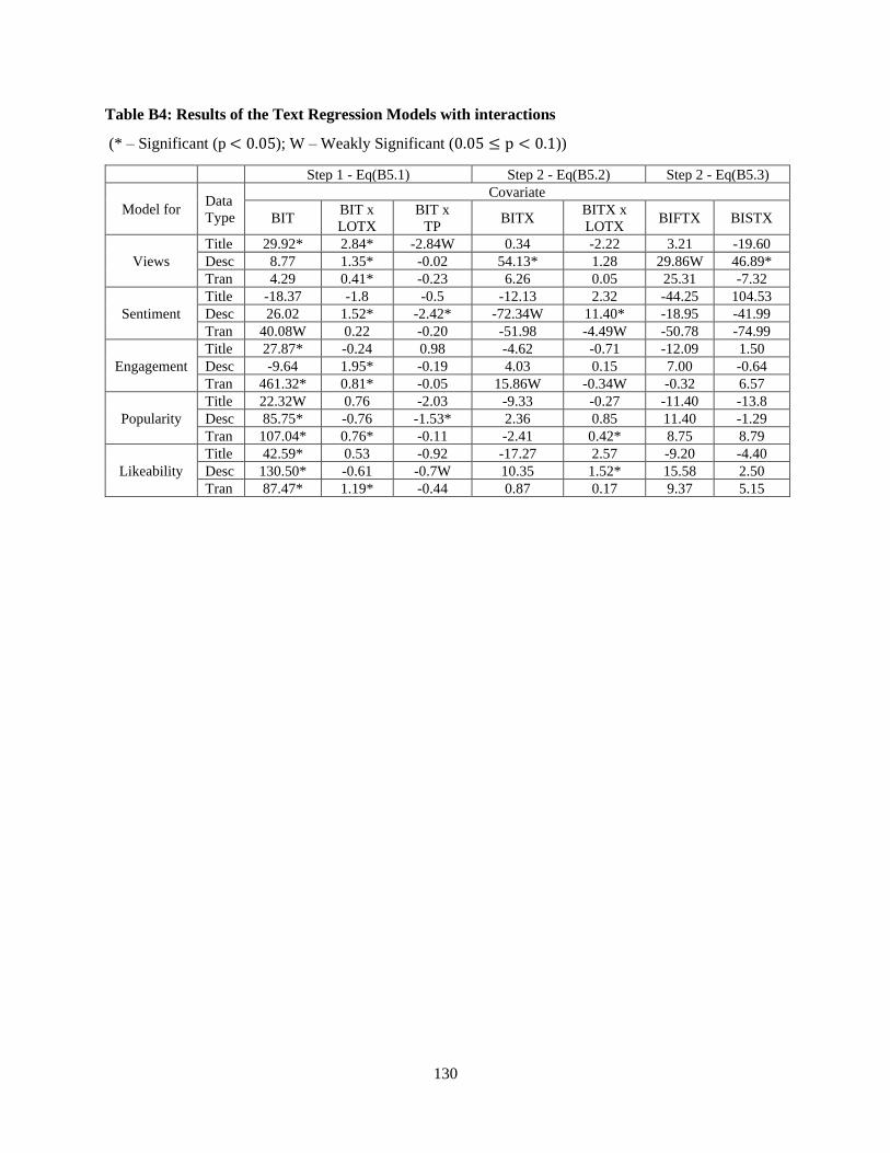
130

Table B4: Results of the Text Regression Models with interactions

(* – Significant (p < 0.05); W – Weakly Significant (0.05 ≤ p < 0.1))

Step 1 - Eq(B5.1) Step 2 - Eq(B5.2) Step 2 - Eq(B5.3)

Model for Data

Type

Covariate

BIT BIT x

LOTX

BIT x

TP BITX

BITX x

LOTX BIFTX BISTX

Views

Title 29.92* 2.84* -2.84W 0.34 -2.22 3.21 -19.60

Desc 8.77 1.35* -0.02 54.13* 1.28 29.86W 46.89*

Tran 4.29 0.41* -0.23 6.26 0.05 25.31 -7.32

Sentiment

Title -18.37 -1.8 -0.5 -12.13 2.32 -44.25 104.53

Desc 26.02 1.52* -2.42* -72.34W 11.40* -18.95 -41.99

Tran 40.08W 0.22 -0.20 -51.98 -4.49W -50.78 -74.99

Engagement

Title 27.87* -0.24 0.98 -4.62 -0.71 -12.09 1.50

Desc -9.64 1.95* -0.19 4.03 0.15 7.00 -0.64

Tran 461.32* 0.81* -0.05 15.86W -0.34W -0.32 6.57

Popularity

Title 22.32W 0.76 -2.03 -9.33 -0.27 -11.40 -13.8

Desc 85.75* -0.76 -1.53* 2.36 0.85 11.40 -1.29

Tran 107.04* 0.76* -0.11 -2.41 0.42* 8.75 8.79

Likeability

Title 42.59* 0.53 -0.92 -17.27 2.57 -9.20 -4.40

Desc 130.50* -0.61 -0.7W 10.35 1.52* 15.58 2.50

Tran 87.47* 1.19* -0.44 0.87 0.17 9.37 5.15

131

Appendix B.6: Interpreting Results for Middle and End of Videos

I interpret the results of the deep learning models on the middle 30 sec and last 30 sec of videos as done in

Section 3.5.2. I focus on all the outcomes except views because, as mentioned in Section 3.3.3, view

count is determined by viewing 30 seconds of a video. This is more likely to be the first 30 seconds unless

viewers immediately skip to other locations in the video for which I have no demonstrated evidence of it

happening on YouTube. I find eight significant results for the Audio model, but no significant results for

the Image and Text model. The results are shown in Table B5.

Table B5: Results from interpreting Regression Models on middle and end of video

Significant increase in attention (A) and

significant increase in outcome (O)

Significant increase in attention (A) but

significant decrease in outcome (O)

Outcome Audio Model Audio Model

Sentiment more speech (without simultaneous music)

in middle 30 sec of audio

A: 2.88%

O: 10.80%

or more music (without simultaneous

speech) in middle 30 sec of audio

A: 3.10%

O: 24.65%

Engagement more music (without simultaneous speech)

in last 30 sec of audio

A: 2.95%

O: - 1.05%

Popularity more speech (without simultaneous music)

in last 30 sec of audio

A: 5.60%

O: 0.07%

more speech (without simultaneous music)

in middle 30 sec of audio

A: 0.98%

O: - 0.21%

or more music (without simultaneous

speech) in middle 30 sec of audio

A: 1.05%

O: - 0.77%

Likeability more speech (without simultaneous music)

in last 30 sec of audio

A: 3.63%

O: 0.26%

or more animal sounds in last 30 sec of

audio

A: 6.60%

O: 1.02%

Overall, the results for the middle and end of audio are qualitatively similar with the results for

the beginning of audio with some differences (e.g., more speech without simultaneous music in the last 30

sec of audio is associated with an increase in popularity which was not found to be true for the first 30 sec

of audio).

132

BIBILIOGRAPHY

Aaker, D. A., & Stayman, D. M. (1990). Measuring audience perceptions of commercials and relating them to ad

impact. Journal of Advertising Research.

ABC. (2014). End Credit Guidelines. Retrieved from

http://www.abc.net.au/tv/independent/doc/ABC_Commissioned_Productions_Credit_Guidelines_2014.pdf

Ailawadi, K. L., Lehmann, D. R., & Neslin, S. A. (2003). Revenue premium as an outcome measure of brand equity.

Journal of Marketing, 67(4), 1-17.

Alammar, J. (2018, June 27). The Illustrated Transformer. Retrieved from http://jalammar.github.io/illustrated-

transformer/

Ameri, M., Honka, E., & Xie, Y. (2019). The Effects of Binge-Watching on Media Franchise Engagement.

Available at SSRN: https://ssrn.com/abstract=2986395 or http://dx.doi.org/10.2139/ssrn.2986395.

Armental, M. (2019, January 10). Amazon’s IMDb Launches Ad-Supported Streaming-Video Service. Retrieved

from https://www.wsj.com/articles/amazons-imdb-launches-ad-supported-streaming-video-service-

11547161586

Athey, S., Tibshirani, J., & Wager, S. (2019). Generalized random forests. The Annals of Statistics, 47(2), 1148-

1178.

Atlas ML. (2020). Image Classification on ImageNet. Retrieved from https://paperswithcode.com/sota/image-

classification-on-imagenet

Bahdanau, D., Cho, K., & Bengio, Y. (2014). Neural machine translation by jointly learning to align and translate.

arXiv preprint arXiv:1409.0473.

Bailis, R. (2020). The State of Influencer Marketing: 10 Influencer Marketing Statistics to Inform Where You

Invest. Retrieved from https://www.bigcommerce.com/blog/influencer-marketing-statistics/#what-is-

influencer-marketing.

Breiman, L. (2001). Random forests. Machine learning, 45(1), 5-32.

Brooks, A. (2020, January 24). As influencers increasingly create video content, what does this mean for brands?

Retrieved from https://marketingtechnews.net/news/2020/jan/24/influencers-increasingly-create-video-

content-what-does-mean-brands/

Burnap, A., Hauser, J. R., & Timoshenko, A. (2019). Design and Evaluation of Product Aesthetics: A Human-

Machine Hybrid Approach. Available at SSRN 3421771.

Cakebread, C. (2017, September 15). Here are all the reasons why Americans say they binge-watch TV shows.

Retrieved from https://www.businessinsider.com/reasons-why-americans-binge-watch-tv-shows-chart-

2017-9

Chae, I., Bruno, H. A., & Feinberg, F. M. (2019). Wearout or weariness? Measuring potential negative

consequences of online ad volume and placement on website visits. Journal of Marketing Research, 56(1),

57-75.

Chakraborty, I., Kim, M., & Sudhir, K. (2019). Attribute Sentiment Scoring with Online Text Reviews: Accounting

for Language Structure and Attribute Self-Selection. Cowles Foundation Discussion Paper No. 2176,

Available at SSRN: https://ssrn.com/abstract=3395012 or http://dx.doi.org/10.2139/ssrn.3395012.

Chen, T., & Guestrin, C. (2016). Xgboost: A scalable tree boosting system. Paper presented at the Proceedings of the

22nd acm sigkdd international conference on knowledge discovery and data mining.

Contestabile, G. (2018). Influencer Marketing in 2018: Becoming an Efficient Marketplace. Retrieved from

https://www.adweek.com/digital/giordano-contestabile-activate-by-bloglovin-guest-post-influencer-

marketing-in-2018/

Cournoyer, B. (2014, March 19). YouTube SEO Best Practices: Titles and Descriptions. Retrieved from

https://www.brainshark.com/ideas-blog/2014/March/youtube-seo-best-practices-titles-descriptions

133

Covington, P., Adams, J., & Sargin, E. (2016). Deep neural networks for youtube recommendations. Paper presented

at the Proceedings of the 10th ACM conference on recommender systems.

Creusy, K. (2016, July 12). What is influencer marketing? Retrieved from https://www.upfluence.com/influencer-

marketing/what-is-influencer-marketing

Danaher, P. J., Lee, J., & Kerbache, L. (2010). Optimal internet media selection. Marketing Science, 29(2), 336-347.

Dawley, S. (2017, May 30). Do Vanity Metrics Matter on Social Media? Yes (And No). Retrieved from

https://blog.hootsuite.com/vanity-metrics/

Deloitte. (2018, March 20). Meet the MilleXZials: Generational Lines Blur as Media Consumption for Gen X,

Millennials and Gen Z Converge. Retrieved from https://www2.deloitte.com/us/en/pages/about-

deloitte/articles/press-releases/digital-media-trends-twelfth-edition.html

Devlin, J., Chang, M.-W., Lee, K., & Toutanova, K. (2018). Bert: Pre-training of deep bidirectional transformers for

language understanding. arXiv preprint arXiv:1810.04805.

Dew, R., Ansari, A., & Toubia, O. (2019). Letting Logos Speak: Leveraging Multiview Representation Learning for

Data-Driven Logo Design. Available at SSRN 3406857.

Dixon, C., & Baig, H. (2019, March 7). What is Youtube comment system sorting / ranking algorithm? . Retrieved

from https://stackoverflow.com/questions/27781751/what-is-youtube-comment-system-sorting-ranking-

algorithm

Dubé, J.-P., Hitsch, G. J., & Manchanda, P. (2005). An empirical model of advertising dynamics. Quantitative

marketing and economics, 3(2), 107-144.

Dubner, S. (2009, May 13). Your Hulu Questions, Answered. Retrieved from

http://freakonomics.com/2009/05/13/your-hulu-questions-answered/

Dzyabura, D., El Kihal, S., & Ibragimov, M. (2018). Leveraging the power of images in predicting product return

rates. Available at SSRN: https://ssrn.com/abstract=3209307 or http://dx.doi.org/10.2139/ssrn.3209307.

Dzyabura, D., & Yoganarasimhan, H. (2018). Machine learning and marketing. In Handbook of Marketing

Analytics: Edward Elgar Publishing.

eMarketer. (2018, August 16). Audience for Connected TV Grows, but Ad Spending Has Lagged. Retrieved from

https://www.emarketer.com/content/audience-for-connected-tv-grows-but-ad-spending-has-lagged

Frederick, S., & Loewenstein, G. (1999). 16 Hedonic Adaptation. Well-Being. The foundations of Hedonic

Psychology/Eds. D. Kahneman, E. Diener, N. Schwarz. NY: Russell Sage, 302-329.

Friedman, J. (2001). Greedy function approximation: a gradient boosting machine. Annals of statistics, 1189-1232.

Friedman, J. (2002). Stochastic gradient boosting. Computational Statistics & Data Analysis, 38(4), 367-378.

Friedman, W. (2017). Shorter-Duration TV Commercials On The Rise. Retrieved from

https://www.mediapost.com/publications/article/308248/shorter-duration-tv-commercials-on-the-rise.html

FTC. (2020). Disclosures 101 for Social Media Influencers. Retrieved from

https://www.ftc.gov/system/files/documents/plain-language/1001a-influencer-guide-508_1.pdf

Gemmeke, J. F., Ellis, D. P., Freedman, D., Jansen, A., Lawrence, W., Moore, R. C., . . . Ritter, M. (2017). Audio

set: An ontology and human-labeled dataset for audio events. Paper presented at the 2017 IEEE

International Conference on Acoustics, Speech and Signal Processing (ICASSP).

Gers, F. A., Schmidhuber, J., & Cummins, F. (1999). Learning to forget: Continual prediction with LSTM.

Gessenhues, A. (2018, June 29). Is YouTube serving up more pre-roll & mid-roll video ads? Retrieved from

https://marketingland.com/is-youtube-serving-up-more-pre-roll-mid-roll-video-ads-243505.

Ghani, J. A., & Deshpande, S. P. (1994). Task characteristics and the experience of optimal flow in human—

computer interaction. The Journal of Psychology, 128(4), 381-391.

Google. (2020a). Add tags to videos. Retrieved from https://support.google.com/youtube/answer/146402?hl=en

Google. (2020b). How video views are counted. Retrieved from

https://support.google.com/youtube/answer/2991785?hl=en

Google. (2020c). Manage ad breaks in long videos. Retrieved from

https://support.google.com/youtube/answer/6175006?hl=en

Google. (2020d). Paid product placements and endorsements. Retrieved from

https://support.google.com/youtube/answer/154235?hl=en

Google. (2020e). Use hashtags for video search. Retrieved from

https://support.google.com/youtube/answer/6390658?hl=en

Graham, M. (2020). Streaming wars will force media companies to choose between pricey subscriptions and ads.

Retrieved from https://www.cnbc.com/2020/01/07/streaming-wars-set-up-fight-between-subscriptions-and-

ad-based-models.html

134

Greenwell, B. M. (2017). pdp: an R Package for constructing partial dependence plots. The R Journal, 9(1), 421-

436.

Hartford, J., Lewis, G., Leyton-Brown, K., & Taddy, M. (2017). Deep IV: A flexible approach for counterfactual

prediction. Paper presented at the Proceedings of the 34th International Conference on Machine Learning-

Volume 70.

Hartmann, J., Heitmann, M., Schamp, C., & Netzer, O. (2020). The Power of Brand Selfies in Consumer-Generated

Brand Imagery. Columbia Business School Research Paper Forthcoming, Available at SSRN:

https://ssrn.com/abstract=3354415 or http://dx.doi.org/10.2139/ssrn.3354415.

Hastie, T., Tibshirani, R., & Friedman, J. (2009). The elements of statistical learning: data mining, inference, and

prediction (2nd ed.): New York: Springer.

Hopf, M. (2020). NLP With Google Cloud Natural Language API. Retrieved from https://www.toptal.com/machine-

learning/google-nlp-tutorial

Howard, A. G., Zhu, M., Chen, B., Kalenichenko, D., Wang, W., Weyand, T., . . . Adam, H. (2017). Mobilenets:

Efficient convolutional neural networks for mobile vision applications. arXiv preprint arXiv:1704.04861.

Hu, J., Shen, L., & Sun, G. (2018). Squeeze-and-excitation networks. Paper presented at the Proceedings of the IEEE

conference on computer vision and pattern recognition.

Hughes, C., Swaminathan, V., & Brooks, G. (2019). Driving Brand Engagement Through Online Social Influencers:

An Empirical Investigation of Sponsored Blogging Campaigns. Journal of Marketing.

Influencer Marketing Hub. (2018, October 24). 4 Factors That Affect Your YouTube Earnings Potential. Retrieved

from https://influencermarketinghub.com/4-factors-affect-youtube-earnings-potential/

Influencer Marketing Hub and CreatorIQ. (2020). The State of Influencer Marketing 2020 : Benchmark Report

Retrieved from https://influencermarketinghub.com/influencer-marketing-benchmark-report-2020/

Ingram, K. (2016, July 7). A brief history of TV shows' opening credit sequences. Retrieved from

http://theweek.com/articles/632836/brief-history-tv-shows-opening-credit-sequences

Ismail, K. (2018, December 10). Social Media Influencers: Mega, Macro, Micro or Nano. cmswire.com. Retrieved

from https://www.cmswire.com/digital-marketing/social-media-influencers-mega-macro-micro-or-nano/

Johnson, L. d. (2019, August 14). Customer Experience Key to Streaming Advertising Success. Retrieved from

https://www.admonsters.com/customer-experience-key-streaming-advertising-success/

Klear (Producer). (2019, April 8, 2020). Inlfuencer Marketing Rate Card. Retrieved from

https://klear.com/KlearRateCard.pdf

Kramer, S. (2018, September 4). The Impact of Influencer Marketing on Consumers. Retrieved from

https://www.themarketingscope.com/influencer-marketing-on-consumers/

Krishnan, S. S., & Sitaraman, R. K. (2013). Understanding the effectiveness of video ads: a measurement study.

Paper presented at the Proceedings of the 2013 conference on Internet measurement conference.

Lambert, B. (2018). YouTube Ads Benchmarks for CPC, CPM, and CTR in Q4 2018. Retrieved from

https://blog.adstage.io/q4-2018-youtube-benchmarks

Lanz, A., Goldenberg, J., Shapira, D., & Stahl, F. (2019). Climb or Jump: Status-Based Seeding in User-Generated

Content Networks. Journal of Marketing Research, 56(3), 361-378.

Lee, D., Manzoor, E., & Cheng, Z. (2018). Focused Concept Miner (FCM): An Interpretable Deep Learning for

Text Exploration. Available at SSRN 3304756.

Lemmens, A., & Croux, C. (2006). Bagging and boosting classification trees to predict churn. Journal of Marketing

Research, 43(2), 276-286.

Li, X., Shi, M., & Wang, X. S. (2019). Video mining: Measuring visual information using automatic methods.

International Journal of Research in Marketing, 36(2), 216-231.

Liu, L., Dzyabura, D., & Mizik, N. (2018). Visual listening in: Extracting brand image portrayed on social media.

Paper presented at the Workshops at the Thirty-Second AAAI Conference on Artificial Intelligence.

Liu, X., Lee, D., & Srinivasan, K. (2019). Large scale cross category analysis of consumer review content on sales

conversion leveraging deep learning. NET Institute Working Paper No. 16-09, Available at SSRN:

https://ssrn.com/abstract=2848528 or http://dx.doi.org/10.2139/ssrn.2848528.

Liu, Y., Ott, M., Goyal, N., Du, J., Joshi, M., Chen, D., . . . Stoyanov, V. (2019). Roberta: A robustly optimized bert

pretraining approach. arXiv preprint arXiv:1907.11692.

Liyakasa, K. (2018). Netflix Will Have Ads, And Other Predictions From Top TV Ad Chiefs. Retrieved from

https://adexchanger.com/digital-tv/netflix-will-ads-predictions-top-tv-ad-chiefs/

Lu, S., Xiao, L., & Ding, M. (2016). A video-based automated recommender (VAR) system for garments.

Marketing Science, 35(3), 484-510.

135

Lu, T., Bradlow, E., & Hutchinson, J. W. (2017). Binge Consumption of Online Content. Carnegie Mellon

University, Working Paper.

Maheshwari, S. (2018, November 11). Are You Ready for the Nanoinfluencers? Retrieved from

https://www.nytimes.com/2018/11/11/business/media/nanoinfluencers-instagram-influencers.html

McGranaghan, M., Liaukonyte, J., & Wilbur, K. C. (2019). Watching people watch TV. Working Paper.

Mediakix. (2020). YouTube Sponsored Videos: Advertising & Influencer Marketing Guide. Retrieved from

https://mediakix.com/influencer-marketing-resources/youtube-sponsored-videos/

Melki, G., Cano, A., Kecman, V., & Ventura, S. (2017). Multi-target support vector regression via correlation

regressor chains. Information Sciences, 415, 53-69.

Miller, L. S. (2017, March 16). Netflix Shouldn’t Let Fans Skip Movie Credits, But We’ll Allow It For TV Shows.

Retrieved from http://www.indiewire.com/2017/05/netflix-skip-intro-bad-for-film-good-for-tv-

1201817946/

Mitchell, A. A. (1986). The effect of verbal and visual components of advertisements on brand attitudes and attitude

toward the advertisement. Journal of consumer research, 13(1), 12-24.

Nededog, J. (2017, March 17). Some lucky Netflix members have a cool new 'skip intro' button to make binge-

watching better. Retrieved from http://www.businessinsider.com/netflix-tests-skip-intro-button-to-improve-

binge-watching-2017-3

Nelson, L. D., Meyvis, T., & Galak, J. (2009). Enhancing the television-viewing experience through commercial

interruptions. Journal of consumer research, 36(2), 160-172.

Neslin, S. A., Gupta, S., Kamakura, W., Lu, J., & Mason, C. H. (2006). Defection detection: Measuring and

understanding the predictive accuracy of customer churn models. Journal of Marketing Research, 43(2),

204-211.

Nevo, A. (2000). A practitioner's guide to estimation of random‐coefficients logit models of demand. Journal of

economics & management strategy, 9(4), 513-548.

O'Connor, C. (2017a, April 10). Earning Power: Here's How Much Top Influencers Can Make On Instagram And

YouTube. Retrieved from https://www.forbes.com/sites/clareoconnor/2017/04/10/earning-power-heres-

how-much-top-influencers-can-make-on-instagram-and-youtube/#a1d07bd24db4

O'Connor, C. (2017b, September 26). Forbes Top Influencers: Meet The 30 Social Media Stars Of Fashion,

Parenting And Pets (Yes, Pets). Retrieved from

https://www.forbes.com/sites/clareoconnor/2017/09/26/forbes-top-influencers-fashion-pets-

parenting/#1a67cea27683

Ogasawara, T. (2011, June 23). Hulu Plus Sort of Available for Android Phones: Hello Android Fragmentation.

Retrieved from https://www.adweek.com/digital/hulu-plus-sort-of-available-for-android-phones-hello-

android-fragmentation/

Olney, T. J., Holbrook, M. B., & Batra, R. (1991). Consumer responses to advertising: The effects of ad content,

emotions, and attitude toward the ad on viewing time. Journal of consumer research, 17(4), 440-453.

Olson, R. S., La Cava, W., Mustahsan, Z., Varik, A., & Moore, J. H. (2017). Data-driven advice for applying

machine learning to bioinformatics problems. arXiv preprint arXiv:1708.05070.

Oughali, M. S., Bahloul, M., & El Rahman, S. A. (2019). Analysis of NBA Players and Shot Prediction Using

Random Forest and XGBoost Models. Paper presented at the 2019 International Conference on Computer

and Information Sciences (ICCIS).

Oxford Dictionary (2018). Definition of binge-watch in US English. Retrieved from

https://en.oxforddictionaries.com/definition/us/binge-watch

Oxford Reference. (2020). influencer. Retrieved from

https://www.oxfordreference.com/view/10.1093/acref/9780191803093.001.0001/acref-9780191803093-e-

630

Parsons, J. (2017, August 24). How Long Until Watching a YouTube Video Counts as a View? Retrieved from

https://growtraffic.com/blog/2017/08/youtube-video-counts-view

Patel, S. (2018, October 1). The anti-Netflix: Free, ad-supported video streaming services are growing. Retrieved

from https://digiday.com/media/free-video-streaming-services-publishers-tv-ambitions/

Pelsmacker, P. D., & Van den Bergh, J. (1999). Advertising content and irritation: a study of 226 TV commercials.

Journal of international consumer marketing, 10(4), 5-27.

Pilakal, M., & Ellis, D. (2020). YAMNet. Retrieved from

https://github.com/tensorflow/models/tree/master/research/audioset/yamnet

Rafieian, O., & Yoganarasimhan, H. (2019). Targeting and Privacy in Mobile Advertising. Available at SSRN:

https://ssrn.com/abstract=3163806 or http://dx.doi.org/10.2139/ssrn.3163806.

136

Rosenberg, E. (2018, October 7). How Youtube Ad Revenue Works. Retrieved from

https://www.investopedia.com/articles/personal-finance/032615/how-youtube-ad-revenue-works.asp

Russakovsky, O., Deng, J., Su, H., Krause, J., Satheesh, S., Ma, S., . . . Bernstein, M. (2015). Imagenet large scale

visual recognition challenge. International journal of computer vision, 115(3), 211-252.

Sahni, N. S. (2015). Effect of temporal spacing between advertising exposures: Evidence from online field

experiments. Quantitative Marketing and Economics, 13(3), 203-247.

Sandler, M., Howard, A., Zhu, M., Zhmoginov, A., & Chen, L.-C. (2018). Mobilenetv2: Inverted residuals and

linear bottlenecks. Paper presented at the Proceedings of the IEEE conference on computer vision and

pattern recognition.

Schneider, S., Baevski, A., Collobert, R., & Auli, M. (2019). wav2vec: Unsupervised pre-training for speech

recognition. arXiv preprint arXiv:1904.05862.

Schweidel, D. A., & Moe, W. W. (2016). Binge watching and advertising. Journal of Marketing, 80(5), 1-19.

Selvaraju, R. R., Cogswell, M., Das, A., Vedantam, R., Parikh, D., & Batra, D. (2017). Grad-cam: Visual

explanations from deep networks via gradient-based localization. Paper presented at the Proceedings of the

IEEE international conference on computer vision.

Sherman, A. (2019). NBC is removing ‘The Office’ from Netflix in 2021 and putting it on its new streaming service.

Retrieved from https://www.cnbc.com/2019/06/25/nbc-to-remove-the-office-from-netflix.html

Sloane, G. (2019). Hulu puts a cap on ad loads. Retrieved from https://adage.com/article/media/hulu-cuts-ad-breaks-

half/317174/

Sommerlad, J. (2018). Netflix will never host advertising or enter battle for live news and sport, ceo says. Retrieved

from https://www.independent.co.uk/life-style/gadgets-and-tech/news/netflix-advertising-live-

broadcasting-mobile-streaming-30-second-trailers-reed-hastings-a8245701.html

Synced. (2017, October 22). Tree Boosting With XGBoost — Why Does XGBoost Win “Every” Machine Learning

Competition? Retrieved from https://medium.com/syncedreview/tree-boosting-with-xgboost-why-does-

xgboost-win-every-machine-learning-competition-ca8034c0b283

Tabor, E. (2020, April 8). Credibility And Trust Are Key To Authentic Influencer Marketing. Retrieved from

https://www.forbes.com/sites/forbesagencycouncil/2020/04/08/credibility-and-trust-are-key-to-authentic-

influencer-marketing/

Tan, M., & Le, Q. V. (2019). Efficientnet: Rethinking model scaling for convolutional neural networks. arXiv

preprint arXiv:1905.11946.

Teixeira, T., Picard, R., & El Kaliouby, R. (2014). Why, when, and how much to entertain consumers in

advertisements? A web-based facial tracking field study. Marketing Science, 33(6), 809-827.

Teixeira, T., Wedel, M., & Pieters, R. (2010). Moment-to-moment optimal branding in TV commercials: Preventing

avoidance by pulsing. Marketing Science, 29(5), 783-804.

Teixeira, T., Wedel, M., & Pieters, R. (2012). Emotion-induced engagement in internet video advertisements.

Journal of Marketing Research, 49(2), 144-159.

Timoshenko, A., & Hauser, J. R. (2019). Identifying customer needs from user-generated content. Marketing

Science, 38(1), 1-20.

Vashishth, S., Upadhyay, S., Tomar, G. S., & Faruqui, M. (2019). Attention interpretability across nlp tasks. arXiv

preprint arXiv:1909.11218.

Vaswani, A., Shazeer, N., Parmar, N., Uszkoreit, J., Jones, L., Gomez, A. N., . . . Polosukhin, I. (2017). Attention is

all you need. Paper presented at the Advances in Neural Information Processing Systems.

West, K. (2013). Unsurprising: Netflix Survey Indicates People Like To Binge-Watch TV. Retrieved from

http://www.cinemablend.com/television/Unsurprising-Netflix-Survey-Indicates-People-Like-Binge-Watch-

TV-61045.html

Widex. (2016, August 9). The human hearing range - what can you hear? Retrieved from

https://www.widex.com/en-us/blog/human-hearing-range-what-can-you-hear

Wu, Y., Schuster, M., Chen, Z., Le, Q. V., Norouzi, M., Macherey, W., . . . Macherey, K. (2016). Google's neural

machine translation system: Bridging the gap between human and machine translation. arXiv preprint

arXiv:1609.08144.

Xie, Q., Hovy, E., Luong, M.-T., & Le, Q. V. (2019). Self-training with Noisy Student improves ImageNet

classification. arXiv preprint arXiv:1911.04252.

Yoganarasimhan, H. (2019). Search personalization using machine learning. Management Science.

YouTube. (2020). What is fair use? Retrieved from https://www.youtube.com/intl/en-GB/yt/about/copyright/fair-

use/#yt-copyright-four-factors

137

Yue-Hei Ng, J., Hausknecht, M., Vijayanarasimhan, S., Vinyals, O., Monga, R., & Toderici, G. (2015). Beyond

short snippets: Deep networks for video classification. Paper presented at the Proceedings of the IEEE

conference on computer vision and pattern recognition.

Zhang, S., Lee, D., Singh, P. V., & Srinivasan, K. (2017). How much is an image worth? Airbnb property demand

estimation leveraging large scale image analytics. Airbnb Property Demand Estimation Leveraging Large

Scale Image Analytics (May 25, 2017).

Zhang, Y., Bradlow, E. T., & Small, D. S. (2015). Predicting customer value using clumpiness: From RFM to

RFMC. Marketing Science, 34(2), 195-208.

Zhao, K., Hu, Y., Hong, Y., & Westland, J. C. (2019). Understanding Factors that Influence User Popularity in Live

Streaming Platforms. Available at SSRN 3388949.

Zimmerman, E. (2016, February 24). Getting YouTube Stars to Sell Your Product. Retrieved from

https://www.nytimes.com/2016/02/25/business/smallbusiness/getting-youtube-stars-to-sell-your-

product.html