Accepted Manuscript

Signal Adaptive Spectral Envelope Estimation for Robust Speech Recognition

Matthias Wölfel

PII: S0167-6393(09)00025-9

DOI: 10.1016/j.specom.2009.02.006

Reference: SPECOM 1787

To appear in: Speech Communication

Received Date: 29 May 2008

Revised Date: 26 January 2009

Accepted Date: 24 February 2009

Please cite this article as: Wölfel, M., Signal Adaptive Spectral Envelope Estimation for Robust Speech Recognition,

Speech Communication (2009), doi: 10.1016/j.specom.2009.02.006

This is a PDF file of an unedited manuscript that has been accepted for publication. As a service to our customers

we are providing this early version of the manuscript. The manuscript will undergo copyediting, typesetting, and

review of the resulting proof before it is published in its final form. Please note that during the production process

errors may be discovered which could affect the content, and all legal disclaimers that apply to the journal pertain.

peer

-005

2412

2, v

ersi

on 1

- 7

Oct

201

0Author manuscript, published in "Speech Communication 51, 6 (2009) 551"

DOI : 10.1016/j.specom.2009.02.006

ACCEPTED MANUSCRIPT

Signal Adaptive Spectral Envelope Estimationfor Robust Speech Recognition

Matthias WolfelInstitut fur Theoretische Informatik, Universitat Karslruhe (TH), Am Fasanengarten 5, 76131 Karlsruhe, Germany

Abstract

This paper describes a novel spectral envelope estimation technique which adapts to the characteristics of the observed signal.This is possible via the introduction of a second bilinear transformation into warped minimum variance distortionless response(MVDR) spectral envelope estimation. As opposed to the first bilinear transformation, however, which is applied in the timedomain, the second bilinear transformation must be applied in the frequency domain. This extension enables the resolution of thespectral envelope estimate to be steered to lower or higher frequencies, while keeping the overall resolution of the estimate and thefrequency axis fixed. When embedded in the feature extraction process of an automatic speech recognition system, it provides forthe emphasis of the characteristics of speech features that are relevant for robust classification, while simultaneously suppressingcharacteristics that are irrelevant for classification. The change in resolution may be steered, for each observation window, by thenormalized first autocorrelation coefficient.

To evaluate the proposed adaptive spectral envelope technique, dubbed warped-twice MVDR, we use two objective functions:class separability and word error rate. Our test set consists of development and evaluation data as provided by NIST for the RichTranscription 2005 Spring Meeting Recognition Evaluation. For both measures, we observed consistent improvements for severalspeaker-to-microphone distances. In average, over all distances, the proposed front–end reduces the word error rate by 4% relativecompared to the widely used mel-frequency cepstral coefficients as well as perceptual linear prediction.

Key words: Adaptive Feature Extraction, Spectral Estimation, Minimum Variance Distortionless Response, Automatic Speech Recognition,

Bilinear Transformation, Time vs. Frequency Domain

1. Introduction

Acoustic modeling in automatic speech recognition(ASR) requires that a windowed speech waveform is re-duced to a set of representative features which preservesthe information needed to determine the phonetic classwhile being invariant to other factors. Those factors mightinclude speaker differences such as fundamental frequency,accent, emotional state or speaking rate, as well as distor-tions due to ambient noise, the channel or reverberation. Inthe traditional feature extraction process of ASR systems,this is achieved through successive feature transformations(e.g. a spectral envelope and/or filterbank followed bycepstral transformation, cepstral normalization and lin-ear discriminant analysis) whereby all phoneme types aretreated equivalently.

Different phonemes, however, have different propertiessuch as voicing where the excitation is due to quasi-periodic opening of the vocal cord or classification relevantfrequency regions [1–3]. While low frequencies are more

relevant for vowels, high frequencies are more relevant forfricatives. It is thus a natural extension to the traditionalfeature extraction approach to vary the spectral resolutionfor each observation window according to some character-istics of the observed signal. To improve phoneme classifi-cation, the spectral resolution may be adapted such thatcharacteristics relevant for classification are emphasizedwhile classification irrelevant characteristics are attenu-ated.

To achieve these objectives, we have proposed to ex-tend the warped minimum variance distortionless response(MVDR) through a second bilinear transformation [4]. Thisspectral envelope estimate has two free parameters to con-trol spectral resolution: the model order, which changes thenumber of linear prediction coefficients, and the warp fac-tor. While the model order allows the overall spectral reso-lution to be changed, the warp factor enables the spectralresolution to be steered to lower or higher frequency regionswithout changing the frequency axis. Note that this is incontrast to the previously proposed warped MVDR [5,6],

Preprint submitted to Elsevier 12 March 2009

peer

-005

2412

2, v

ersi

on 1

- 7

Oct

201

0

ACCEPTED MANUSCRIPT

wherein the warp factor has an influence on both the spec-tral resolution and the frequency axis.

A note about the differences between the present publi-cation and [4] is perhaps now in order. The present pub-lication presents important background information whichhad been discarded in the conference publication [4] be-cause of space limitations including: A comparison of wellknown and not so well known ASR front-ends on close anddistant recordings in terms of word error rate and class sep-arability. The present publication also includes a detailedanalysis and discussion of phoneme confusability. In addi-tion it fosters understanding by highlighting the differencesbetween warping in the time and frequency domain and in-vestigating of the values of the steering function in relationto single phonemes and phoneme classes.

The balance of this paper is organized as follows. Abrief review of spectral envelope estimation techniqueswith a focus on MVDR is given in Section 2. The bilineartransformation is reviewed in Section 3 where its prop-erties in the time and frequency domains are discussed.Section 4 introduces a novel adaptive spectral estima-tion technique, dubbed warped-twice MVDR, and a fastimplementation thereof. A possible steering function, toemphasize phoneme relevant spectral regions, is discussedin Section 5. The proposed signal-adaptive feature extrac-tion scheme is evaluated in Section 6. Our conclusions arepresented in the final section of this paper.

2. MVDR Spectral Envelope

In the feature extraction stage of speech recognition sys-tems, particular characteristics of the spectral estimate arerequired. To name a few: provide a particular spectral reso-lution, be robust to noise, and model the frequency responsefunction of the vocal tract during voiced speech. To satisfythese requirements, both non-parametric and parametricmethods have been proposed. Non-parametric methods arebased on periodograms, such as power spectra, while para-metric methods such as linear prediction estimate a smallnumber of parameters from the data. Table 1 summarizesthe characteristics of different spectral estimation meth-ods. Two widely used methods in ASR are mel-scale powerspectrum [7] and warped or perceptual linear prediction [8].

In order to overcome the problems associated with(warped or perceptual) linear prediction, namely over-estimation of spectral power at the harmonics of voicedspeech, Murti and Rao [9,10] proposed the use of min-imum variance distortionless response (MVDR), whichis also known as Capon’s method [11] or the maximum-likelihood method [12], for all-pole modeling of speech in1997. They demonstrated that MVDR spectral envelopescope well with the aforementioned problem. Some yearslater, in 2001, MVDR was applied to speech recognitionby Dharanipragada and Rao [13]. To account for the fre-quency resolution of the human auditory system, we haveintroduced warped MVDR [5,6]. It extends the MVDR

Table 1

Properties of spectral estimation methods.PS = power spectrum; LP = linear prediction;

MVDR = minimum variance distortionless response∗ no particular name is given in the work by Nakatoh et al.

Spectral Estimate Properties

detail resolution sensitive to pitch

PS exact linear, static very high

mel-scale PS [15] smooth mel, static high

LP [16,17] approx. linear, static medium

perceptual LP [8] approx. mel, static medium

warped LP [18,19] approx. mel, static medium

warped-twice LP∗ [20] approx. mel, adaptive medium

MVDR [9,10,13] approx. linear, static low

warped MVDR [6] approx. mel, static low

perceptual MVDR [14] approx. mel, static low

warped-twice MVDR approx. mel, adaptive low

approach by warping the frequency axis with a bilineartransformation in the time domain.

In this section, we briefly review MVDR spectral estima-tion. A detailed discussion of speech spectral estimation byMVDR can be found in [10], with focus on speech recog-nition and warped MVDR in [6], and with focus on robustfeature extraction for recognition in [14].

MVDR methodology

MVDR spectral estimation can be posed as a problem infilterbank design, wherein the final filterbank is subject tothe distortionless constraint [21]:

The signal at the frequency of interest ωfoi must pass undis-torted with unity gain.

Hfoi(ejωfoi) =M∑

k=0

hfoi(k)e−jkωfoi = 1, (1)

where the impulse response hfoi(k) of the distortionless fi-nite impulse responce filter of order M is specifically de-signed to minimize the output power. Defining the fixedfrequency vector

v(ejω) = [1, e+jω, . . . , e+jMω]T (2)

allows the constraint to be rewritten in vector form as

vH(ejωfoi) · hfoi = 1, (3)

where (•)H represents the Hermitian transpose operatorand

hfoi = [hfoi(0), hfoi(1), . . . , hfoi(M)]T (4)

is the distortionless filter.Upon defining the autocorrelation sequence

R[n] =L−n∑m=0

x[m]x[m− n] (5)

2

peer

-005

2412

2, v

ersi

on 1

- 7

Oct

201

0

ACCEPTED MANUSCRIPT

of the input signal x of length L as well as the (M + 1) ×(M + 1) Toeplitz autocorrelation matrix R whose (l, k)th

element is given by

Rl,k = R[l − k], (6)

it is readily shown that hfoi can be obtained by solving theconstrained minimization problem:

minhfoi

hTfoi Rhfoi subject to vH(ejωfoi)hfoi = 1. (7)

The solution to this problem is given by [21]:

hfoi =R−1 v(ejωfoi)

vH(ejωfoi)R−1 v(ejωfoi). (8)

This implies that hfoi is the impulse response of the distor-tionless filter for the frequency ωfoi. The MVDR envelope ofthe power spectrum of the signal P (ejω) at frequency ωfoi

is then obtained as the output of the optimized constrainedfilter:

SMVDR(ejωfoi) =12π

∫ π

−π

∣∣Hfoi(ejω)∣∣2 P (ejω)dω. (9)

Although MVDR spectral estimation was posed as a distor-tionless filter design for a given frequency ωfoi, the MVDRspectrum can be represented in parametric form for all fre-quencies [21]

SMVDR(ejω) =1

vH(ejω)R−1v(ejω). (10)

Fast computation of the MVDR envelope

Assuming that the (M +1)×(M +1) Hermitian Toeplitzcorrelation matrix R is positive definite and thus invert-ible, Musicus [12] derived a fast algorithm to calculate theMVDR spectrum from a set of linear prediction coefficients(LPCs). The steps (i until iii) of Musicus’ algorithm [12]are:

(i) Computation of the LPCs a(M)0···M of order M includ-

ing the prediction error variance εM

(ii) Correlation of the LPCs

µk =

1

εM

M−k∑m=0

(M + 1− k − 2m)a(M)m a

∗(M)m+k , k ≥ 0

µ∗−k , k < 0(11)

(iii) Computation of the MVDR envelope

SMVDR(ejω) =1∑M

m=−M µme−jωm. (12)

(iv) Scaling of the MVDR envelopeIn order to improve robustness to additive noise ithas been argued in [6] to adjust the highest spectralpeak of the MVDR envelope to match to the highestspectral peak of the power spectrum to get the socalled scaled envelope.

0.4447

0.3624

Nor

mal

ized

Fre

quen

cy S

cale 1.0

0.0

0.2

0.4

0.6

0.8

20 1 3 4Frequency (kHz)

0.6254

0.4595

40 2 6 8Frequency (kHz)

0.44470.3624

Nor

mal

ized

Fre

quen

cy S

cale

1.0

0.0

0.2

0.4

0.6

0.8

20 1 3 4Frequency (kHz)

0.6254

0.4595

40 2 6 8Frequency (kHz)

40 2 6 8Frequency (kHz)

Mel

Fre

quen

cy

Bili

near

App

roxi

mat

ion

0

2

4

86

0

2

4

86

Mel

Fre

quen

cy

Bili

near

App

roxi

mat

ion

0

2

4

86

0

2

4

86

Frequency (kHz)40 2 6 8

Fig. 1. Mel-frequency (scale shown along left edge) can be approx-imated by a bilinear transformation (scale shown along right edge)

demonstrated for a sampling rate of 16 kHz, αmel = 0.4595.

3. Warping — Time vs. Frequency Domain

In the speech recognition community it is well knownthat features based on a non-linear frequency mapping im-prove the recognition accuracy over features on a linear fre-quency scale [7]. Transforming the linear frequency axis ωto a non-linear frequency axis ω is called frequency warping.One way to achieve frequency warping is to apply a non-linear scaled filterbank, such as a mel-filterbank, to the lin-ear frequency representation. An alternative possibility isto use a conformal mapping such as a first order all-pass fil-ter, also known as a bilinear transformation [22,23], whichpreserves the unit circle. The bilinear transformation is de-fined in the z-domain as

z−1 =z−1 − α

1− α · z−1∀ − 1 < α < +1, (13)

where α is the warp factor. The relationship between ω andω is non-linear as indicated by the phase function of theall-pass filter [19]

arg(e−jω

)= ω = ω + 2 arctan

(α sinω

1− α cos ω

). (14)

The mel-scale, which along with the Bark scale is one ofthe most popular non-linear frequency mappings, was pro-posed by Stevens et al. in 1937 [15]. It models the non-linearpitch perception characteristics of the human ear and iswidely applied in audio feature extraction. A good approx-imation of the mel-scale by the bilinear transformation ispossible, if the warp factor is set accordingly. The optimalwarp factor depends on the sampling frequency and can befound by different optimization methods [24]. Fig. 1 com-pares the mel-scale with the bilinear transformation for asampling frequency of 16 kHz.

Frequency warping by bilinear transformation can eitherbe applied in the time domain or in the frequency domain.In both cases, the frequency axis is non-linearly scaled;however, the effect on the spectral resolution differs for thetwo domains. This effect can be explained as follows:– Warping in the time domain modifies the values in the

autocorrelation matrix and therefore, in the case of linear

3

peer

-005

2412

2, v

ersi

on 1

- 7

Oct

201

0

ACCEPTED MANUSCRIPT

0 842 6Frequency (kHz)

751 3

Fig. 3. The plot of two warped-twice MVDR spectral envelopes

demonstrates the effect of spectral tilt. While the spectral tilt isnot compensated for the dashed line, it is compensated for the solid

line. It is clear to see that high frequencies are emphasized if no

compensation is applied.

prediction, more linear prediction coefficients are used,for α > 0, to describe lower frequencies and less coeffi-cients to describe higher frequencies.

– Warping in the frequency domain does not change thespectral resolution as the transformation is applied afterspectral analysis. As indicated by Nocerino et al. [25],a general warping transformation in the same domain,such as the bilinear transformation, is equivalent to amatrix multiplication

fwarp[n] = L(α)f [n],

where the matrix L(α) depends on the warp factor. Itfollows that the values fwarp[n] on the warped scale are alinear interpolation of the values f [n] on the linear scale.In the case of linear prediction or MVDR, the predictioncoefficients are not altered as they are calculated beforethe bilinear transformation is applied.

Fig. 2 demonstrates the effect of warping applied eitherin the time or in the frequency domain on the spectralenvelope and compares the warped spectral envelopes withthe unwarped spectral envelope.

For clarity we briefly investigate the change of spectralresolution, for the most interesting case, where the bilineartransformation is applied in the time domain with warp fac-tor α > 0. In this case we observe that spectral resolutiondecreases as frequency increases. In comparison to the res-olution provided by the linear frequency scale, α = 0, thewarped frequency resolution increases for low frequenciesup to the turning point frequency [26]

ftp(α) = ± fs

2πarccos(α), (15)

where fs represents the sampling frequency. At the turn-ing point frequency, the spectral resolution is not affected.Above the turning point frequency, the frequency resolu-tion decreases in comparison to the resolution provided bythe linear frequency scale. For α < 0, spectral resolutionincreases as frequency increases.

As observed by Strube [18], prediction error minimiza-tion of the predictors am in the warped domain is equiva-lent to the minimization of the output power of the warpedinverse filter

A(z) = 1 +M∑

m=1

amz−m(z) (16)

in the linear domain, where each unit delay element z−1 isreplaced by a bilinear transformation z−1. The predictionerror is therefore given by

E(ejω) = |A(ejω)|2P (ejω), (17)

where P (ejω) is the power spectrum of the signal. The totalprediction error power can be expressed as

σ2 =∫ π

−π

E(ejω)dω =∫ π

−π

E(ejω) W 2(ejω)dω (18)

with

W (z) =√

1− α2

1− αz−1. (19)

The minimization of the prediction error σ2, however, doesnot lead to minimization of the power, but minimizationof the power of the error signal filtered by the weightingfilter W (z), which is apparent from the presence of thisfactor in (18). Thus, the bilinear transformation introducesan unwanted spectral tilt. To compensate for this negativeeffect, we apply the inverted weighting function∣∣∣W (z) · W (z−1)

∣∣∣−1

=

∣∣1 + α · z−1∣∣2

1− α2. (20)

The effect of the spectral tilt of the bilinear transformationand the remedy by (20) are depicted in Fig. 3.

4. Warped-Twice MVDR Spectral Envelope

The use of two bilinear transformations, one in time do-main and the other in frequency domain, introduces twoadditional free parameters into the MVDR approach [4].The first free parameter, the model order, is already deter-mined by the underlying linear prediction model. Due tothe application of two bilinear transformations which ap-ply two warping stages into MVDR spectral estimation, theproposed approach is dubbed warped-twice MVDR. Whilethe model order varies the overall spectral resolution of theestimate, which becomes apparent by comparing the dif-ferent envelopes for model order 30, 60 and 90 in Fig. 4a,the warp factors bend the frequency axis as already seen inSection 3. Bending the frequency axis can be used to applythe mel-scale or, when done on a speaker-dependent basis,to implement vocal tract length normalization (VTLN), al-though the latter is not used in the experiments describedin Section 6, as piece-wise linear warping leads to betterresults [27].

As already mentioned in Section 1, our aim is to changethe spectral resolution while keeping the frequency axisfixed. This becomes possible by compensating for the un-wanted bending of the frequency axis, introduced by thefirst warping stage in the time domain, by a second warp-ing stage in the frequency domain. An example is given inFig. 4b.

4

peer

-005

2412

2, v

ersi

on 1

- 7

Oct

201

0

ACCEPTED MANUSCRIPT

Frequency (kHz)0 842 6 751 3

Frequency (kHz)0 842 6751 3

Changed Resolution

Frequency (kHz)0 842 6751 3

No WarpingWarping in Time Domain Warping in Frequency Domain

0 842 6Frequency (kHz)

751 3 0 842 6Frequency (kHz)

751 3 0 842 6Frequency (kHz)

751 3

(a) (b) (c)

Changed Resolution

Same Resolution

Same Resolution

Fig. 2. Warping in (a) time domain, (b) no warping and (c) warping in frequency domain. While warping in the time domain is changing thespectral resolution and frequency axis, warping in frequency domain does not alter the spectral resolution but still changes the frequency axis.

0 842 6Frequency (kHz)

751 3

Warp

(b)

0.3

0.6

0 842 6Frequency (kHz)

751 3

Model Order

(a)

30

90

Fig. 4. The solid lines show warped-twice MVDR spectral envelopes with model order 60, α = 0.4595 and αmel = 0.4595 which, except forthe spectral tilt, are identical to a warped MVDR spectral envelope. Its counterparts with lower and higher (a) model order and (b) warpfactor α are given by dashed lines. The arrows point in the direction of higher resolution. While the model order changes the overall spectralresolution at all frequencies, the warp factor moves spectral resolution to lower or higher frequencies. At the turning point frequency, the

resolution is not affected and the direction of the arrows changes.

Fast computation of the warped-twice MVDR envelope

A fast computation of the warped-twice MVDR enve-lope of model order M is possible by extending Musicus’algorithm. A flowchart diagram of the individual process-ing steps is given in Fig. 5.

(i) Computation of the warped autocorrelationcoefficients R[0] · · · R[M + 1]

To compute warped autocorrelation coefficients, thelinear frequency axis ω has to be transformed toa warped frequency axis ω by replacing the unitdelay element z−1 with a bilinear transformation(13). This leads to the warped autocorrelation coef-ficients [28,19]

5

peer

-005

2412

2, v

ersi

on 1

- 7

Oct

201

0

ACCEPTED MANUSCRIPT

BilinearTransformation

Autocorrelation

Compensationfor Spectral Tilt

Levinson-DurbinRecursion

Correlation ofwarped LPC

Warped-MVDR

CompensationWarp Factor

Windowed Time Signal

Warped-Twice MVDR

Warp Factor

BilinearTransformation

ConcatenatedWarp Factor

Fig. 5. Overview of warped-twice minimum variance distortionlessresponse. Symbols are defined as in the text.

R[n] =L−n−1∑

m=0

x[m]yn[m] (21)

where yn[m] is the sequence of length L given by

yn[m] = α ·(yn[m−1]−yn−1[m])−yn−1[m−1] (22)

and initialized with y0[m] = x[m].Note that we need to calculate M + 1 warped au-

tocorrelation coefficients (the additional coefficient isused in the compensation step).

(ii) Calculation of the compensation warp factorTo fit the final frequency axis to the mel-scale, we needto compensate for the first warping stage with valueα in a second warping stage with the warp factor

β =α− αmel

1− α · αmel. (23)

(iii) Compensation for the spectral tiltTo compensate for the distortion introduced by theconcatenated bilinear transformations with warp fac-tors α and β, we first concatenate the cascade of warp-ing stages into a single warping stage with the warpfactor

χ =α + β

1 + α · β. (24)

A derivation of (24) is provided in [29]. To get a flattransfer function, we now apply the inverted weight-ing function

∣∣∣W (z) · W (z−1)∣∣∣−1

(25)

to the warped autocorrelation coefficients, which canbe realized as a second order finite impulse responsefilter:

R[m] =1 + χ2 + χ · R[m− 1] + χ · R[m + 1]

1− χ2. (26)

(iv) Computation of the warped LPCs a(M)0···M including the

warped prediction error variance εM

The warped LPCs can now be estimated using theLevinson-Durbin recursion [30], by replacing the lin-ear autocorrelation coefficients R with their warpedand spectral tilt compensated counterparts R.

(v) Correlation of the warped LPCsThe MVDR parameters µ−k can be related to theLPC by

µk =

1

εM

M−k∑m=0

(M + 1− k − 2m)a(M)m a

∗(M)m+k , k ≥ 0

µ∗−k , k < 0(27)

(vi) Computation of the warped-twice MVDR envelopeThe spectral estimate can now be obtained by

SW2MVDR(ejω) =1∑M

m=−M µmejω−β

1−β·ejω

. (28)

Note that the spectrum (28), if β is set appropri-ately, is already resembling the non-linear frequencyaxis as discussed in Section 3. In those cases it isnecessary to either:(a) eliminate the non-linear spaced triangular filter-

bank as for example used in the extraction ofmel-frequency cepstral coefficients or perceptuallinear prediction coefficients, or

(b) replace the non-linear spaced triangular filter-bank by a filterbank of uniform half-overlappingtriangular filters in order to provide feature re-duction and additional spectral smoothing.

(vii) Scaling of the warped-twice MVDR envelopeTo provide more robustness we match the warped-twice MVDR envelope to the highest spectral peakof the power spectrum.

Implementation Issues

Frequency warping including linear or non-linear VTLNcan be realized using filterbanks. Carefully adjusted, thosefilterbanks can simulate the bilinear transformation in thefrequency domain. In the case of warped-twice MVDR spec-tral estimation those filterbanks can be adjusted for eachindividual frame according to the compensation warp fac-tor β and the VTLN parameter. In practice it is sufficient to

6

peer

-005

2412

2, v

ersi

on 1

- 7

Oct

201

0

ACCEPTED MANUSCRIPT

use a limited number of pre-calculated filterbanks; in thisway, warped-twice MVDR spectral estimation can be im-plemented with only a very small overhead when comparedto warped MVDR spectral estimation.

5. Steering Function

To support automatic speech recognition, the free pa-rameters of the warped-twice MVDR envelope have to beadapted in such a way that classification relevant charac-teristics are emphasized while less relevant information issuppressed. Nakatoh et al. [20] proposed a method for steer-ing the spectral resolution to lower or higher frequencieswhereby for every frame i, the first two autocorrelation co-efficients were used to define the steering function

ϕi =Ri[1]Ri[0]

. (29)

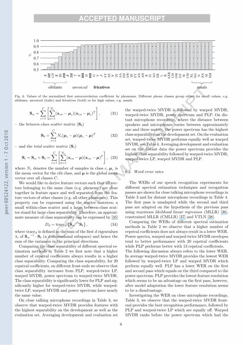
The zero autocorrelation coefficient R[0] represents the av-erage power while the first autocorrelation coefficient R[1]represents the correlation of a signal. Thus ϕ has a highvalue for voiced signals and a low value for unvoiced signals.Fig. 6 gives the different values of the normalized first auto-correlation coefficient ϕ averaged over all samples for eachindividual phoneme. A clear separation between the frica-tives and non-fricatives can be observed. Fricatives are con-sonants produced by forcing air through a narrow channelmade by placing two articulators close together. The sibi-lants are a particular subset of fricatives made by directinga jet of air through a narrow channel in the vocal tract to-wards the sharp edge of the teeth. Sibilants are louder thantheir non-sibilant counterparts, and most of their acousticenergy occurs at higher frequencies than by non-sibilantfricatives. A detailed discussion about the properties of dif-ferent phoneme classes can be found in [1].

To adjust for the sensitivity to the steering function thefactor γ is introduced, and the subtraction of the bias ϕ =1I

∑i ϕi (i.e., the mean over all values I in the training set)

keeps the average of α close to αmel. This leads to

αi = γ · (ϕi − ϕ) + αmel. (30)

The last equation is a slight modification of the originalformulation proposed by Nakatoh et al. As preliminary ex-periments have revealed that the word accuracy is not verysensitive to γ, we kept γ fixed at 0.1; values around 0.1might lead to slightly, however, not significantly differentresults. The influence of γ has been, in more detail, inves-tigated in [20].

6. Evaluation

To evaluate the proposed warped-twice MVDR spectralestimation and steering function against traditional front-ends such as perceptual linear prediction (PLP) [8], melfrequency cepstral coefficients (MFCC) [7] and more re-cently proposed front-ends based on warped-twice LP or

warped MVDR spectral envelopes, we used NIST’s devel-opment and evaluation data of the Rich Transcription 2005Spring Meeting Recognition Evaluation [31]. The data hasbeen chosen as a test environment as it contains challeng-ing acoustic environments on both close and distant speechrecordings. The development data, sampled at 16 kHz,consists of 5 seminars with approximately 130 minutes ofspeech. The evaluation data, also sampled at 16 kHz, con-sists of 16 seminars with approximately 180 minutes ofspeech. The data was collected under the Computers in theHuman Interaction Loop (CHIL) project [32] and containsspontaneous, native and non-native speech.

We have used the Janus Recognition Toolkit (JRTk).To train acoustic models only relatively little supervisedin-domain speech data is available. Therefore, we decidedto train the acoustic models on close talking channels ofmeeting corpora and the Translanguage English Database(TED) corpus [33], summing up to a total of approximately100 hours of acoustic training material. After split andmerge training the acoustic model consisted of approxi-mately 3,500 context-dependent codebooks with up to 64diagonal covariance Gaussians each, summing up to a totalof 180,000 Gaussians.

Each front-end provided features every 10 ms (first andsecond pass) or 8 ms (third pass). Spectral estimates havebeen obtained by the Fourier transformation (MFCC),PLP, warped MVDR, warped-twice LP and warped-twiceMVDR spectral estimation. While the Fourier transfor-mation is followed by a mel-filterbank, warped MVDR,warped-twice LP and warped-twice MVDR are followedby a linear filterbank. The 30 (13 or 20 in the case of PLP)spectral features have been truncated to 13 or 20 cepstralcoefficients after cosine transformation. After mean andvariance normalization, the cepstral features were stacked(seven adjacent left and right frames providing either 195or 300 dimensions) and truncated to the final featurevector dimension of 42 by a multiplication with the opti-mal feature space matrix (the linear discriminant analysismatrix multiplied with the global semi-tied covariancetransformation matrix [34]).

To train a four-gram language model, we used cor-pora consisting of broadcast news, proceedings of con-ferences such as ICSLP, Eurospeech, ICASSP, ACL andASRU and talks in TED. The vocabulary contains ap-proximately 23,000 words, the perplexity is 120 with anout-of-vocabulary rate of 0.25%.

We compare the different front-ends on class separabilityand word error rate (WER).

6.1. Class Separability

Class separability is a classical concept in pattern recog-nition, usually expressed using a scatter matrix. We candefine– the within-class scatter matrix (Sw)

7

peer

-005

2412

2, v

ersi

on 1

- 7

Oct

201

0

ACCEPTED MANUSCRIPT

S

SH

CH FJH T

HH

DH Y AY

V AA

AW

ZHZ

TH K D G P AE

IX EH

AX

IH R AO L

AX

R

OW W XL NEY

AH

IY ER B UH

OY

UW

NG

XN

XMM

0.5

0.6

0.8

0.9

1.0

0.7

sibilants nasalsfricativesunvoiced

Fig. 6. Values of the normalized first autocorrelation coefficient by phonemes. Different phone classes group either for small values, e.g.

sibilants, unvoiced (italic) and fricatives (bold) or for high values, e.g. nasals.

Sw =C∑

c=1

[Nc∑

n=1

(xcn − µc)(xcn − µc)T

], (31)

– the between-class scatter matrix (Sb)

Sb =C∑

c=1

Nc(µc − µ)(µc − µ)T (32)

– and the total scatter matrix (St)

St = Sw + Sb =C∑

c=1

[Nc∑

n=1

(xcn − µ)(xcn − µ)T

], (33)

where Nc denotes the number of samples in class c, µc isthe mean vector for the cth class, and µ is the global meanvector over all classes C.

We would like to derive feature vectors such that all vec-tors belonging to the same class (e.g. phoneme) are closetogether in feature space and well separated from the fea-ture vectors of other classes (e.g. all other phonemes). Thisproperty can be expressed using the scatter matrices; asmall within-class scatter and a large between-class scat-ter stand for large class separability. Therefore, an approxi-mate measure of class separability can be expressed by [35]

Dd = traced

Sw

−1Sb

, (34)

where traced is defined as the sum of the first d eigenvaluesλi of Sw

−1 · Sb (a d-dimensional subspace) and hence thesum of the variances in the principal directions.

Comparing the class separability of different spectral es-timation methods in Table 2 we first note that a highernumber of cepstral coefficients always results in a higherclass separability. Comparing the class separability, for 20cepstral coefficients, on different front-ends we observe thatclass separability increases from PLP, warped-twice LP,warped MVDR, power spectrum to warped-twice MVDR.The class separability is significantly lower for PLP and sig-nificantly higher for warped-twice MVDR, while warped-twice LP, warped MVDR and power spectrum have nearlythe same value.

On close talking microphone recordings in Table 3, weobserve that warped-twice MVDR provides features withthe highest separability on the development as well as theevaluation set. Averaging development and evaluation set

the warped-twice MVDR is followed by warped MVDR,warped-twice MVDR, power spectrum and PLP. On dis-tant microphone recordings, where the distance betweenspeakers and microphones varies between approximatelyone and three meters, the power spectrum has the highestclass separability on the development set. On the evaluationset, warped-twice MVDR performs equally well as warpedMVDR, see Table 4. Averaging development and evaluationset on the distant data the power spectrum provides thehighest class separability followed by warped-twice MVDR,warped-twice LP, warped MVDR and PLP.

6.2. Word error rates

The WERs of our speech recognition experiments fordifferent spectral estimation techniques and recognitionpasses are shown for close talking microphone recordings inTable 3 and for distant microphone recordings in Table 4.The first pass is unadapted while the second and thirdpass are adapted on the hypothesis of the previous passusing maximum likelihood linear regression (MLLR) [36],constrained MLLR (CMLLR) [37] and VTLN [38].

Comparing the WERs of different spectral estimationmethods in Table 2 we observe that a higher number ofcepstral coefficients does not always result in a lower WER.Power spectra, warped and warped-twice MVDR envelopestend to better performance with 20 cepstral coefficientswhile PLP performs better with 13 cepstral coefficients.The following discussion always refers to the lower WER.In average warped-twice MVDR provides the lowest WERfollowed by warped-twice LP and warped MVDR whichperform equally well. PLP has a lower WER on the firstand second pass which equals on the third compared to thepower spectrum. PLP provides the lowest feature resolutionwhich seems to be an advantage on the first pass, however,after model adaptation the lower feature resolution seemsto be a disadvantage.

Investigating the WER on close microphone recordings,Table 3, we observe that the warped-twice MVDR front-end provides the best recognition performance, followed byPLP and warped-twice LP which are equally off. WarpedMVDR ranks before the power spectrum which had the

8

peer

-005

2412

2, v

ersi

on 1

- 7

Oct

201

0

ACCEPTED MANUSCRIPT

Table 3Class separability and word error rates for different front-end types and settings on close microphone recordings

Spectrum Model Cepstra Class Separability Word Error Rate %

Test Set Train Develop Eval Develop Eval

Pass 1 2 3 1 2 3

power spectrum – 13 11.007 16.470 16.088 36.1 30.3 28.0 35.3 29.7 27.7

power spectrum – 20 11.620 17.929 16.299 36.0 29.7 27.7 37.2 31.3 28.4

PLP 13 13 10.699 17.110 15.152 34.7 29.3 27.2 34.2 29.6 27.1

PLP 20 20 11.029 18.059 16.068 34.7 29.5 27.7 34.9 30.3 27.9

warped MVDR 60 13 10.768 16.813 16.261 35.0 30.0 28.2 35.5 29.9 27.6

warped MVDR 60 20 11.337 18.022 16.614 34.5 29.1 27.3 35.3 29.6 27.3

warped-twice LP 20 13 10.772 17.038 16.254 35.3 30.5 28.5 36.2 29.8 27.1

warped-twice LP 20 20 11.333 17.864 16.436 34.4 29.5 27.4 37.1 29.4 26.8

warped-twice MVDR 60 13 10.893 17.673 16.456 34.5 29.5 27.5 34.1 29.2 27.0

warped-twice MVDR 60 20 11.473 18.510 16.818 34.1 28.8 26.8 35.4 29.0 26.3

Table 4Class separability and word error rates for different front-end types and settings on distant microphone recordings

Spectrum Model Cepstra Class Separability Word Error Rate %

Test Set Train Develop Eval Develop Eval

Pass 1 2 3 1 2 3

power spectrum – 13 11.007 14.786 13.470 61.9 52.0 51.1 60.8 54.2 51.1

power spectrum – 20 11.620 15.806 13.944 59.8 50.4 48.9 61.0 55.0 51.7

PLP 13 13 10.699 15.121 12.917 60.7 51.8 50.5 59.9 53.4 51.8

PLP 20 20 11.029 15.399 12.975 59.8 52.1 50.2 59.6 54.4 52.7

warped MVDR 60 13 10.768 13.836 13.885 62.9 53.7 52.0 60.7 52.8 50.7

warped MVDR 60 20 11.337 14.487 14.161 60.9 51.2 49.7 59.6 51.7 49.5

warped-twice LP 20 13 10.772 14.524 13.393 62.8 53.8 52.1 61.1 54.5 50.9

warped-twice LP 20 20 11.333 15.119 13.803 58.9 50.8 49.3 59.9 53.0 50.2

warped-twice MVDR 60 13 10.893 14.895 13.901 63.1 53.6 51.6 60.7 52.7 49.3

warped-twice MVDR 60 20 11.473 15.380 14.116 60.3 51.1 49.8 59.9 50.4 47.9

lowest recognition performance.On distant microphone recordings, Table 3, the warped-

twice MVDR front-end shows robust performance and has,in average, the lowest WER. On the development set, how-ever, the power spectrum has the lowest WER. In averagethe warped-twice MVDR is followed by warped MVDR,then warped-twice LP, thereafter the power spectrum dueto a weak performance on the evaluation set and PLP onthe last place.

The reduced improvements of the warped-twice MVDRin comparison to the warped MVDR on distant recordingscan be explained by the fact that, in comparison to closetalking microphone recordings, the range of the values ϕi

over all i is reduced. Therefore, the effect of spectral resolu-tion steering is attenuated and consequently warped-twiceMVDR envelopes behave more similarly to warped MVDRenvelopes.

6.3. Phoneme Confusability

We investigate the confusability between phonemes bycalculating the minimum distances, on the final features,between different phoneme pairs. In order to account for therange of variability of the sample points in both phonemeclasses Ωp and Ωq, expressed by the covariance matrices Σp

and Σq, we extend the well known Mahalanobis distanceby a second covariance matrix

Dp,q =√

(µp − µq)T (Σp + Σq)−1 (µp − µq).

Here µp denotes the sample mean of phoneme class Ωp andµq denotes the sample mean of phoneme class Ωq respec-tively.

As the comparison of the confusion matrix itself wouldbe impractical, we limit our investigations on the compar-ison of the distance between the nearest phoneme to agiven phoneme for different spectral estimation techniques

9

peer

-005

2412

2, v

ersi

on 1

- 7

Oct

201

0

ACCEPTED MANUSCRIPT

Table 5Nearest phoneme distance for different phonemes (ordered by ϕ) and spectral estimation methods.

phoneme S SH CH Z JH ZH F TH T K · · · OW OY W UW XL NG N XN M XM

ϕ 0.51 0.55 0.60 0.62 0.73 0.78 0.80 0.81 0.85 0.89 · · · 0.97 0.97 0.97 0.98 0.98 0.98 0.98 0.98 0.98 0.98

spectrum power spectrum

nearest Z CH JH S CH JH T T TH P · · · XL OW B UH L N M N N L

distance 2.41 1.56 0.81 2.27 1.36 1.55 2.36 2.04 1.75 2.33 · · · 3.19 3.55 3.04 2.97 2.94 3.32 2.83 3.59 3.04 4.88

spectrum warped MVDR

nearest Z CH JH S CH JH T T TH P · · · XL AY B UH L N M N N XL

distance 2.32 1.56 0.86 2.21 1.65 1.49 2.26 2.03 1.74 2.36 · · · 3.49 3.8 3.29 3.19 3.18 3.52 3.01 3.65 3.3 5.07

spectrum warped-twice LP

nearest Z CH JH S CH JH K T TH P · · · XL OW B UH L N M N N XL

distance 2.46 1.58 0.87 2.26 1.78 1.5 2.38 2.09 1.72 2.37 · · · 3.22 3.47 3.06 2.93 2.96 3.36 2.77 3.57 3.03 4.97

spectrum warped-twice MVDR

nearest Z CH JH S CH JH T T TH P · · · XL OW B UH L N M N N XL

distance 2.43 1.6 0.85 2.24 1.75 1.58 2.35 2.08 1.74 2.35 · · · 3.26 3.59 3.1 2.99 3 3.36 2.83 3.56 3.12 5.02

Table 2

Average class separability and average word error rates for differentfront-end types and sanity checksMO: model order, CC: number of cepstral coefficients, CS: class

separability

Spectrum MO CC CS Word Error Rate %

Pass 1 2 3

power spectrum – 13 15.204 48.5 41.6 39.5

power spectrum – 20 15.995 48.5 41.6 39.2

PLP 13 13 15.075 47.4 41.0 39.2

PLP 20 20 15.625 47.3 41.6 39.6

warped MVDR 60 13 15.199 48.5 41.6 39.6

warped MVDR 60 20 15.821 47.6 40.4 38.5

warped-twice LP 20 13 15.302 48.9 42.1 39.6

warped-twice LP 20 20 15.806 47.6 40.7 38.4

warped-twice MVDR 60 13 15.731 48.1 41.3 38.9

warped-twice MVDR 60 20 16.206 47.4 39.8 37.7

as plotted in Tabel 5. Note that the PLP front-end is ex-cluded from this analysis as it, due to a different scale,can not be directly compared. By comparing the nearestphoneme pairs over different phonemes and spectral esti-mation methods we observe that different spectral repre-sentations result in slightly different phoneme pairs. In ad-dition we observe that, in average, phonemes with a smallvalue of ϕ are easier confused (smaller distance) with otherphonemes than phonemes with a high ϕ value. This can beexplained by the energy of the different phoneme classeswhere the phoneme classes belonging to small ϕ values con-tain less energy and are thus stronger distorted by back-ground noise.

Comparing the power spectrum with the warped MVDRenvelope we observe that the power spectrum tends toprovide lower confusability for lower ϕ values and higher

confusability for higher ϕ values. The warped-twice LPand warped-twice MVDR envelopes have a similar distancestructure over ϕ, with in average larger distances for thewarped-twice MVDR envelopes. While the warped-twiceMVDR envelope, compared to the warped MVDR enve-lope, provides a lower confusability for small values of ϕ,the confusability is higher for larger values of ϕ. While thewarped MVDR envelope is not capable to provide a lowerconfusability over the whole range of ϕ in comparison to thepower spectrum, the warped-twice MVDR envelope pro-vides, in average, a lower confusability over the whole rangeof ϕ in comparison to the power spectrum.

7. Conclusion

We have introduced warped-twice MVDR spectral es-timation by extending warped MVDR estimation with asecond bilinear transformation. With these extensions, itis possible to steer spectral resolution to lower or higherfrequencies while keeping the overall resolution of the esti-mate and the frequency axis fixed. We have demonstratedone possible application in the front-end of a speech-to-text system by steering the resolution of the spectral en-velope to classification relevant spectral regions. The pro-posed framework showed consisted improvements in termsof class separability and WER on a large vocabulary speechrecognition task on close talk as well as on distant speechrecordings. Further improvements might be expected by amore suitable steering function.

References

[1] J. Olive, Acoustics of American English speech : A dynamic

approach, Springer, 1993.

10

peer

-005

2412

2, v

ersi

on 1

- 7

Oct

201

0

ACCEPTED MANUSCRIPT

[2] N. Mesgarani, S. David, S. Shamma, Representation of phonemes

in primary auditory cortex: Howthe brain analyzes speech, Proc.

of ICASSP (2007) 765–768.

[3] V. Driaunys, K. Rudzionis, P. Zvinys, Analysis of vocal

phonemes and fricative consonant discrimination based onphonetic acoustics features, Information Technology and Control

34 (3) (2005) 257–262.

[4] M. Wolfel, Warped-twice minimum variance distortionless

response spectral estimation, Proc. of EUSIPCO (2006) .

[5] M. Wolfel, J. McDonough, A. Waibel, Minimum variancedistortionless response on a warped frequency scale, Proc. of

Eurospeech (2003) 1021–1024.

[6] M. Wolfel, J. McDonough, Minimum variance distortionless

response spectral estimation, review and refinements, IEEE

Signal Processing Magazine 22 (5) (2005) 117–126.

[7] S. Davis, P. Mermelstein, Comparison of parametric represen-

tations for monosyllable word recognition in continuouslyspoken sentences, IEEE Trans. on Acoustics, Speech and Signal

Processing 28 (4) (1980) 357–366.

[8] H. Hermansky, Perceptual linear predictive (PLP) analysis of

speech, J. Acoustic. Soc. Am. 87 (4) (1990) 1738–1752.

[9] M. Murthi, B. Rao, Minimum variance distortionless response

(MVDR) modeling of voiced speech, Proc. of ICASSP (1997)

1687–1690.

[10] M. Murthi, B. Rao, All-pole modeling of speech based on

the minimum variance distortionless response spectrum, IEEETrans. on Speech and Audio Processing 8 (3) (2000) 221–239.

[11] J. Capon, High-resolution frequency-wavenumber spectrumanalysis, Proc. of the IEEE 57 (1969) 1408–1418.

[12] B. Musicus, Fast MLM power spectrum estimation from

uniformly spaced correlations, IEEE Trans. on Acoustics,Speech, and Signal Processing 33 (1985) 1333–1335.

[13] S. Dharanipragada, B. Rao, MVDR based feature extraction forrobust speech recognition, Proc. of ICASSP (2001) 309–312.

[14] S. Dharanipragada, U. Yapanel, B. Rao, Robust featureextraction for continuous speech recognition using the MVDR

spectrum estimation method, IEEE Trans. Speech and Audio

Processing 15 (1) (2007) 224–234.

[15] S. Stevens, J. Volkman, E. Newman, The mel scale equates

the magnitude of perceived differences in pitch at differentfrequencies, J. Acoust. Soc. Am. 8 (3) (1937) 185–190.

[16] G. U. Yule, On a method of investigating periodicities indisturbed series, with special reference to wolfers sunspot

numbers, Phil. Trans. Roy. Soc. 226–A (1927) 267–298.

[17] J. Makhoul, Linear prediction: A tutorial review, Proc. of the

IEEE 63 (4) (1975) 561–580.

[18] H. Strube, Linear prediction on a warped frequency scale, J.Acoustic. Soc. Am. 68 (8) (1980) 1071–1076.

[19] H. Matsumoto, M. Moroto, Evaluation of mel-LPC cepstrumin a large vocabulary continuous speech recognition, Proc. of

ICASSP (2001) 117–120.

[20] Y. Nakatoh, M. Nishizaki, S. Yoshizawa, M. Yamada, An

adaptive mel-LP analysis for speech recognition, Proc. of ICSLP(2004) .

[21] S. Haykin, Adaptive filter theory—3th ed., Prentice Hall, 1991.

[22] A. Oppenheim, D. Johnson, K. Steiglitz, Computation of spectra

with unequal resolution using the fast fourier transform, IEEE

Proc. Letters 59 (2) (1971) 229–301.

[23] C. Braccini, A. V. Oppenheim, Unequal bandwidth spectral

analysis using digital frequency warping, IEEE Trans. Acoust.,Speech, Signal Processing 22 (1974) 236–244.

[24] J. O. Smith III, J. S. Abel, Bark and ERB bilinear transforms,

IEEE Trans. on speech and audio processing 7 (6) (1999) 697–708.

[25] N. Nocerino, F. Soong, L. Rabiner, D. Klatt, Comparative studyof several distortion measures for speech recognition, Proc. of

ICASSP (1985) 25–28.

[26] A. Harma, U. Laine, A comparison of warped and conventional

linear predictive coding, IEEE Trans. on Speech and Audio

Processing 9 (5) (2001) 579–588.[27] M. Wolfel, Mel-Frequenzanpassung der Minimum Varianz

Distortionless Response Einhullenden, Proc. of ESSV (2003) 22–

29.[28] M. Matsumoto, Y. Nakatoh, Y. Furuhata, An efficient mel-LPC

analysis method for speech recognition, Proc. of ICSLP (1998)

1051–1054.[29] A. Acero, Acoustical and environmental robustness in automatic

speech recognition, Ph.D. thesis, Carnegie Mellon University

(September 1990).[30] A. Oppenheim, R. Schafer, Discrete-time signal processing,

Prentice-Hall Inc., 1989.

[31] NIST, Rich transcription 2005 spring meeting recognitionevaluation, www.nist.gov/speech/tests/rt/rt2005/spring.

[32] Computers in the human interaction loop, http://chil.server.de.[33] Linguistic Data Consortium (LDC), Translanguage english

database, www.ldc.upenn.edu/Catalog/LDC2002S04.html.

[34] M. Gales, Semi-tied covariance matrices for hidden Markovmodels, IEEE Trans. Speech and Audio Processing 7 (1999)

272–281.

[35] R. Haeb-Umbach, Investigations on inter-speaker variability inthe feature space, Proc. of ICASSP (1999) 397 – 400.

[36] C. Leggetter, P. Woodland, Maximum likelihood linear

regression for speaker adaptation of continuous density hiddenMarkov models, Computer Speech and Language 9 (2) (1995)

171–185.

[37] M. J. F. Gales, Maximum likelihood linear transformationsfor HMM-based speech recognition, Computer Speech and

Language 12 (1998) 75–98.[38] L. Welling, H. Ney, S. Kanthak, Speaker adaptive modeling

by vocal tract normalization, IEEE Trans. Speech and Audio

Processing 10 (6) (2002) 415–426.

11

peer

-005

2412

2, v

ersi

on 1

- 7

Oct

201

0