Analog Integrated Circuits and Signal Processing manuscript No.(will be inserted by the editor)

J.-F. Bercher · C. Berland

Envelope and Phase delays correction in an EER radio architecture

Received: March 30, 2007 / Revised: date

Abstract This article deals with synchronization in the En-velope Elimination and Restoration (EER) type of transmit-ter architecture. To illustrate the performances of such so-lution, we choose to apply this architecture to a 64 carriers16QAM modulated OFDM. We first introduce the problem-atic of the realisation of a highly linear transmitter. We thenpresent the Envelope Elimination and Restoration solutionand draw attention to its major weakness: a high sensitivityto desynchronization between the phase and envelope signalpaths. To address this issue, we propose an adaptive synchro-nization algorithm relying on a feedback loop, a Least MeanSquare formulation and involving an interpolation step. Itenables the correction of delay mismatches and tracking ofpossible variations. We demonstrate that the quality of theinterpolator has a direct impact on Error Vector Magnitude(EVM) value and output spectrum. Implementation detailsare provided along with an analysis of the behaviour andperformances of the method. We present HPADS and Mat-lab simulation results and then focus on the enhancement ofthe transmitter performances using the proposed algorithm.

1 Introduction

Recent radiocommunication systems aiming at high data rateare based on efficient modulation schemes in which Quadra-ture Amplitude Modulations (QAM) are obviously preferredto frequency or phase modulation. While the 3GPP standardemploys QPSK and 16QAM, higher data rate are achieved(in WLAN system for example) using Orthogonal FrequencyData Multiplexing (OFDM) modulation. Although these mod-ulations are suitable for signal processing, the realization ofthe RF front end, particularly the transmitter, becomes moreand more complex.In the conception of a transmitter, it is essential to achieve

J.-F. Bercher and C. BerlandESYCOM-ESIEE, Université Paris-EstCité Descartes, BP99, 93162 Noisy-le-Grand Cedex, FranceTel.: +33-1-45926642Fax: +33-1-45926699E-mail: {jf.bercher,c.berland}@esiee.fr

both efficiency and linearity. In radiocommunication stan-dards, the quality of the transmitted signal is well defined,usually in terms of output spectrum, Adjacent Channel PowerRatio (ACPR) and Error Vector Magnitude (EVM). Whenthe modulated signal presents an envelope variation, similarto an amplitude modulated signal, the compression effect ofthe Power Amplifier (PA) generates intermodulation prod-ucts which directly impact the three mentioned figures ofmerit. This implies that with a classic class A PA, the in-put signal would have to present a mean power (dependingon the type of modulation) lower than the input compres-sion point: the difference is quantified in terms of back off.In order to gain in efficiency, a linearization system is oftenpreferred to a linear amplification.In this paper, we deal with theEnvelope Elimination andRestoration(EER) principle, and illustrate it in the case of a16QAM 64 carriers OFDM modulation. The EER principlewas proposed by Kahn in 1952 [14] and is based on the split-ting of a modulated signal into two signals. The first one isa constant envelope phase modulated signal, while the sec-ond one is the envelope of the original signal. In the originalEER transmitter, the splitting is realized in an analog way us-ing a limiter and an envelope detector. The phase modulatedsignal is the input of an efficient PA whereas the envelopesignal is sent to a switching power supply which feeds thelast stage of the PA. The transmitter now evoluates toward afully digital transmitter [23] as shown in Fig.1.

OFDM

Modulator

I

Q

CORDIC

Processor

Envelope

Frequency

RF out

-1.0 -0.5 0.0 0.5 1.0-1.5 1.5

-1.0

-0.5

0.0

0.5

1.0

-1.5

1.5

Power

Supply

Modulated phase

locked Loop

Fig. 1 Polar transmitter using a CORDIC processor

2 J.-F. Bercher, C. Berland

The digital creation of the two signals is achieved using aCORDIC processor [22]. The principle of this processor re-lies on the rotation of a vector(Xi ,Yi) to a new vector. Inour case, the final vector is(Zi ,θ), whereZi is the magni-tude of the vector and the rotation angle is our phase. VLSIimplementation can profit from of a suitable iterative formu-lation. The phase signal is sent to the PA amplifier using amodulated PLL. This solution is preferred to a I/Q RF mod-ulator in order to reduce transmitted spurious emissions. Tolimit distortion, the envelope signal is usually amplified witha class S modulator using aΣ∆ modulator rather than a clas-sic PWM. The final amplification is realized by a high effi-ciency amplifier. As the input signal is a constant envelopesignal, switched class of power amplifiers are preferred dueto their high efficiency. As demonstrated in [20], the class Epower amplifier is very suitable for this application since theexpression of the output voltage is directly proportionnaltoits power supply. This property is mandatory as we intend toreinject the envelope variation through the modulation of itspower supply.However the main drawback of this architecture is its sensi-tivity to delay mismatch between the two signals.The delays introduced by the two paths can be mismatcheddue to pipeline differences in the paths and the delay inthe anti-alias filter (amplitude path), as well as small con-tributions from other analog delays [21]. Furthermore, in aproduction environment, delays should be matched to varia-tions in process including supply voltage, frequency, outputpower and temperature [18]. This usually requires carefulfactory calibration procedures. The mismatch deterioratesboth the EVM and the output spectrum of the transmittedsignal [4; 24] and has to be corrected. A linear interpola-tion was suggested in [11] to compensate for the mismatch,while a group delay equalizer was proposed in [17]. In thesetwo cases, it still remains to identify the delay mismatch andtrack its possible variations. In this article, we propose ascheme and an associated algorithm that covers the wholecalibration problem: identification, correction and tracking.In the first part, we demonstrate the sensitivity of EER ap-plied to a 16QAM 64 carriers OFDM modulation and bringforward the maximum tolerable delay mismatch for this mod-ulation. The second part presents an efficient algorithm whichcorrects this default. We then focus on the implementationof the algorithm and on the importance of the interpolationfilter used to resynchronize the signals. In the final part, ananalysis of the behaviour and performances of the algorithmis provided. Simulation results performed on HPADS arepresented and show the performances achieved with this so-lution in terms of output spectrum, EVM and ACPR.

2 Impact of delay mismatches on an OFDM modulation

Using a 16QAM 64 carriers OFDM modulation is an in-teresting case study for the validation of this kind of ar-chitecture because of its high Peak to Average Power Ra-tio (PAPR). In fact, for an OFDM modulation, the PAPR

Table 1 ACPR obtained for different delay mismatches. It is evalu-ated for the full 64 carriers 20MHz OFDM modulation, with a channelspacing of 25MHz.

Delay T/27 T/13 T/5 T/3ACPR (dB) -37 -29.7 -20.7 -15.7

is equal to the number of carriers, which corresponds to10log(64) = 18dB in our simulation case. A few results havealready been presented on the study of the whole transmit-ter with this modulation [2] and this paper indicates that thecritical specification is the synchronization of signals. Fig. 2and Fig.3 present the impact of delay mismatch in the rangeof ±T

3 , with T the time symbol, on the output spectrum andon the EVM. Table 1 gives the values of ACPR for thesedelays. The symbol rate is 20MHz.

2320 2340 2360 2380 2400 2420 2440 2460 24802300 2500

-60

-40

-20

0

-80

20

Frequency

Outp

ut

spectr

um

T/13

T/27

T/3

T/5

Fig. 2 Impact of the delay mismatch on output spectrum (taken in200kHz bandwidth)

-0.3 -0.2 -0.1 0.0 0.1 0.2 0.3-0.4 0.4

0.05

0.10

0.00

0.15

Delay

EV

m r

ms

Fig. 3 Impact of the delay mismatch on the EVM

It is important to notice that the EVM calculation for OFDMmodulations must be realized on each carrier separately andthen averaged. Fig.4 shows that the effect of the desynchro-nization on the first subcarrier for delaysT/27 andT/5 actsas additional noise.

Envelope and Phase delays correction in an EER radio architecture 3

-1.3

-1.1

-0.9

-0.7

-0.5

-0.3

-0.1

0.1

0.3

0.5

0.7

0.9

1.1

1.3

-1.5

1.5

-1.0

-0.5

0.0

0.5

1.0

-1.5

1.5

Constellation

-1.3

-1.1

-0.9

-0.7

-0.5

-0.3

-0.1

0.1

0.3

0.5

0.7

0.9

1.1

1.3

-1.5

1.5

-1.0

-0.5

0.0

0.5

1.0

-1.5

1.5

Constellation

Fig. 4 Impact of the delay mismatch on the constellation for T/27 andT/5

As a guideline, we take specifications from 802.11.a stan-dard: the rms EVM is specified at a maximum of 11.22%and the output spectrum has to remain under -40dBc abovea 30MHz frequency offset from the carrier measured in a1MHz resolution bandwidth. When analysing the EVM re-sults, we can observe that a desynchronization ofT/3 pro-duces an EVM value of 14% and when considering the out-put spectrum, in 1MHz bandwidth, the value at 30MHz fromthe carrier is about -7.5dBc. In fact, the value of -40dBc isonly obtained for a delay ofT/27 which gives an EVM valueof about 0.6% This demonstrates that the synchronization ofsignals impacts so strongly on the output spectrum that it ismandatory to implement a correction algorithm.

3 The correction algorithm

This paper is an extended version of [3] where we presenteda preliminary version of the algorithm. In this version, thealgorithm is presented in more details and implementationissues are discussed. More specifically, we discuss the role,performances and implementation of the interpolation stepand provide a detailed analysis of the algorithm performances.

3.1 Envelope and phase alignment

According to the central limit theorem, for complex modu-lation schemes such as the OFDM, when the number of sub-carriers is large, the emitted signal can be approximated asa gaussian distributed complex random variable. For a nar-rowband stationary signal written as

ξ (t) = x(t)cos(ω0t)+y(t)sin(ω0t) (1)

it is well known thatRxx(τ) = Rxy(τ) and thatRxy(τ) =−Ryx(τ), whereRxx and Rxy are respectively the autocor-relation and intercorrelation functions. The processesx(t)andy(t) are always uncorrelated at the same instant, that isRxy(0) = 0. If ξ (t) is normal, thenx(t) andy(t) are indepen-dent at the same instant. The complex gaussian processξ (t)is completely characterized by its mean and autocorrelationfunction

Rξ ξ (τ) = Rxx(τ)cos(ω0τ)+Rxy(τ)sin(ω0τ). (2)

Let us denoteSξ ξ ( f ) andSxx( f ) the spectra ofξ (t) andx(t),that is the Fourier transforms of the autocorrelation functionsRξ ξ (τ) andRxx(τ). WhenSξ ξ ( f ) is symmetric with centralfrequencyf0, the in-phase and quadrature componentsx(t)andy(t) are uncorrelated, that isRxy(τ) = 0. The basebandspectrumSxx( f ) is generally proportional to the square ofthe transfer function of the emission filter, which shall beshaped as a square-root Nyquist filter. Consequently, the au-tocorrelation functionRxx(τ) = Ryy(τ), which is the inverseFourier transform of the baseband spectrum, is the impulseresponseh of a (full) Nyquist filter. The processξ (t) canalso be written as

ξ (t) = ρ(t)cos(ω0t −φ(t)) (3)

whereρ(t) is the envelope andφ(t) is the phase process,with

{

x(t) = ρ(t)cos(φ(t)),y(t) = ρ(t)sin(φ(t)).

In the case of a complex gaussian process, it is well knownthat the envelope and phase are independentat the sameinstant and respectively distributed according to the Ray-leigh and uniform distributions. The case of delayed enve-lope and phase is less known. In fact, it appears that forgaussian processes, the envelopeρ(t) and phaseφ(t − ∆ )are also Rayleigh and uniform distributed, and arealwaysindependent (see [4]) with no reference to the correlationcoefficient, whatever the delay between envelope and phasecomponents. In consequence, the output do not convey anyinformation on the time alignment or mismatch between theenvelope and phase components. As a result, it isnot pos-sible to correct the relative delay between the envelope andphase components from the sole observation of the systemoutput. Calibration then needs to rely on a feedback loop andinvolve a direct comparison between the initial “aligned”signal and the observed signal.In a calibration step without data transmission, we can alsomodify the modulation scheme and design non-gaussian se-quences with some dependence between envelope and phase.In such a situation, a ‘contrast’ based on the output proper-ties may be devised in order to align the components. How-ever, we will focus here on the feedback solution that pre-serves the data and modulation technique.

3.2 The compensation algorithm

Let us denotez(t) the output of the system. Due to the delays∆1 and∆2 that affect the envelope and phase components,we have

z(t) = ρ(t −∆1)cos(ω0t −φ(t −∆2))

= ρ(t −∆1)cos(φ(t −∆2))cos(ω0t)

+ρ(t −∆1)sin(φ(t −∆2))sin(ω0t) .

We propose here to correct the delays using an adaptive pre-compensation. The synchronization algorithm relies on the

4 J.-F. Bercher, C. Berland

idea of introducing two advancesµ1 andµ2 in order to prec-ompensate the delays, as illustrated in Fig.5. In such a case,the output becomes

z(t) = ρ(t + µ1−∆1)cos(ω0t −φ(t + µ2−∆2)) (4)

and we will adjust the advancesµ1 andµ2 in order to min-imize a statistical distance betweenz(t) andξ (t). A naturalcriterion is the minimization of the quadratic distance

J(µ1,µ2; t) = E[

|ξ (t)−z(t)|2]

, (5)

where E[•] is the statistical expectation operator. This ex-pression can also be rewritten as

J(µ1,µ2; t) = E[

ex(t)2]cos(ω0t)2+E

[

ey(t)2]sin(ω0t)

2

+E[ex(t)ey(t)]sin(2ω0t)

where ex(t) and ey(t) are the errors for the in-phase andquadrature components respectively,

ex(t) = (ρ(t)cosφ(t)−ρ(t1)cosφ(t2)) (6a)

ey(t) = (ρ(t)sinφ(t)−ρ(t1)sinφ(t2)) (6b)

and where, in order to simplify the expressions, we noted

t1 = t + µ1−∆1 andt2 = t + µ2−∆2. (7)

After time averaging, this simply reduces to

J(µ1,µ2) =12

{

Jx(µ1,µ2)+Jy(µ1,µ2)}

(8)

with

Jx(µ1,µ2) = E[

ex(t)2] andJy(µ1,µ2) = E

[

ey(t)2]. (9)

The global criterion equals the sum of two elementary cri-teria on the in-phase and quadrature components. We canreadily obtain the same criterion (up to a factor) using thedemodulated, baseband, version of the signal.In practice, we indeed work in baseband with digital signals.After sampling, we compare the digital input signal to thesampled baseband output. In the following, we will keepTfor the symbol period and noteTs the sampling period. Con-sequently, we will note the different discrete time indexesasfollow

t(n) = nTst1(n) = nTs+ µ1−∆1t2(n) = nTs+ µ2−∆2.

(10)

The output sampling clock does not need to be synchronousto the input: it may be a divided version of the input clock,and any propagation delay will be absorbed in the correctionprocedure.Since it is simpler to generate delayed signals than advancedsignals, we introduce a small processing delayD in Fig. 5.

ρ(t+µ1-∆1)

φ(t+µ2-∆2)

RF Transmitterρ(t+µ1)

φ(t+µ2)

ρ(t)cos(φ(t)) ρ(t+µ1-∆1)cos(φ(t+µ2-∆2))

+ −

ρ(n)

φ(n)µ1,µ2z-D

ρ(t)sin(φ(t)) ρ(t+µ1-∆1)sin(φ(t+µ2-∆2))

Fig. 5 Principle of delays correction.

Let us consider the criterionJx(µ1,µ2) in (9) on the in-phasecomponent. Developing and taking into account the inde-pendence betweenρ(t1) andφ(t2) lead to

Jx(µ1,µ2) = 2Cx(0,0)−2Cx(µ1−∆1,µ2−∆2) (11)

where

Cx(τ1,τ2) = E[ρ(t)cos(φ(t))ρ(t − τ1)cos(φ(t − τ2))](12)

with τ = 1= µ1−∆1 andτ2 = µ2−∆2, is a kind of ‘correla-tion function’. The termCx(0,0) simply reduces toCx(0,0)=E[

ρ(t)2]

E[

cos(φ(t))2]

= Rxx(0), the variance of the in-phasex(t) component. It is important to note thatCx(τ,τ), ob-tained withτ1 = τ2 = τ is nothing else but the correlationfunctionRxx(τ). Since we know that the correlation functionis proportional to the shaping filterh, it appears that the be-haviour of the criterionJx(µ1,µ2) is closely related to theshaping filter. Regarding the quadrature component and cri-terionJy(µ1,µ2), the same conclusions and formulas foundin (11,12) are easily obtained by substitutingx by y and cosby sin.In the case of an OFDM modulation, the criterionJ(τ1,τ2)was evaluated numerically by Monte-Carlo simulations witha square root Nyquist filter (square root raised cosine with0.5 roll-off). This is illustrated in Fig.6 for delays (advances)between−4T and 4T. We can recognize here the generalshape of the (inverted) impulse response of a raised cosine,somewhat distorded and modulated. The criterion does notonly present a global minimum atτ1 = 0, τ2 = 0, but alsoseveral other minima. Derivation of a closed-form formulafor criteria (9) involving (12) is a challenging if not impos-sible task. However, in Fig.7, where the criterion for delaysless than 1.5T is shown, we clearly observe that any descentalgorithm will avoid local minima for delays∆1,∆2 ≤ T,with initial conditions set to zero.

3.3 Gradient algorithm

Since we do not have a closed-form for the criterion nor adirect explicit solution for its global minimizer, we need toexhibit the solution using a descent algorithm. We simply

Envelope and Phase delays correction in an EER radio architecture 5

−4−2

02

4

−4

−2

0

2

40

0.1

0.2

0.3

0.4

0.5

Envelope delayPhase delay

Fig. 6 Shape of the criterion for the envelope and phase delays∈[−4T,4T], with T the symbol period. The shape of the criterion is re-lated to the impulse response of the shaping filter and presents localminima.

−10

1

−1

0

1

0

0.1

0.2

0.3

0.4

Envelope delayPhase delay

Fig. 7 Shape of the criterion for the envelope and phase delays∈[−3T/2,3T/2], with T the symbol period.

use a gradient algorithm that consists in iterating the follow-ing formulas:

µ1(n+1) = µ1(n)− γ1(n) ∂J(µ1,µ2)∂ µ1

∣

∣

∣

µ1=µ1(n)

µ2(n+1) = µ2(n)− γ2(n) ∂J(µ1,µ2)∂ µ2

∣

∣

∣

µ2=µ2(n)

(13)

whereγ1(n) andγ2(n) are two adaptation steps that possiblydepend on the iteration indexn. The gradients are given by

∂J(µ1,µ2)

∂• =12

[

∂Jx(µ1,µ2)

∂• +∂Jy(µ1,µ2)

∂•

]

(14)

and we readily obtain

∂Jx(µ1,µ2)

∂ µ1= −E

[

dρ(u)

du

∣

∣

∣

∣

u=t1(n)

cosφ(t2(n))ex(t(n))

]

(15a)

∂Jy(µ1,µ2)

∂ µ1= −E

[

dρ(u)

du

∣

∣

∣

∣

u=t1(n)

sinφ(t2(n))ey(t(n))

]

(15b)

and

∂Jx(µ1,µ2)

∂ µ2= −E

[

dcosφ(u)

du

∣

∣

∣

∣

u=t2(n)

ρ(t1(n))ex(t(n))

]

(16a)

∂Jy(µ1,µ2)

∂ µ2= −E

[

dsinφ(u)

du

∣

∣

∣

∣

u=t2(n)

ρ(t1(n))ey(t(n))

]

(16b)

with ex andey defined by (6a,6b).The update equations are obtained using these gradients in(13). However, we do not have the analytical expressionsof the statistical expectations involved in these formulas.Therefore, we have to resort to using a stochastic approx-imation of these theoretical recursions. A popular solutionin adaptive filtering is theLeast Mean Squares(LMS) algo-rithm that simply consists in omitting the statistical expec-tation. The LMS then involves theinstantaneous gradientrather than the (correct) statistical average. Furthermore, theequations are updated at each new sample. This gives

µ1(n+1) = µ1(n)+ γ1(n)dρ(u)

du

∣

∣

∣

∣

t1(n)

×(

cos(φ(t2(n)))ex(t)+sinφ(t2(n))ey(t(n)))

(17)

µ2(n+1) = µ2(n)+ γ2(n)ρ(t1(n))×(

dcosφ(u)

du

∣

∣

∣

∣

t2(n)

ex(t)+dsinφ(u)

du

∣

∣

∣

∣

t2(n)

ey(t(n))

)

. (18)

Practical implementation of formulas (17) and (18) requires

– computation of the errorsex(t(n)) andey(t(n)) definedin (6a) and (6b) which results from the comparison ofthe system input and output,

– computation of the derivatives that can be simply ap-proximated by finite differences ofρ(t1(n)) and cos(φ(t2(n))).

Of course, the algorithm can be simplified by consideringa sole error component rather than two. For instance, onecan simply putey = 0 in the previous equations. In practice,simulations show that the gain associated with the secondcomponent is extremely small.

6 J.-F. Bercher, C. Berland

For formulas (17) and (18), the computational load is about 8real multiplications per iteration. However, since the deriva-tives must be computed at timet1(n) and t2(n), that is atthe output of the corrected system,ρ(t) and cos(φ(t)) mustbe separately accessible. This implies a quadrature demod-ulation before the feedback loop. Furthermore, with this ap-proach, we need to adjust two advancesµ1,µ2 and applythem to the input signal. Adopting very high sampling fre-quencies in order to get the required precision may not bean efficient solution. Digital interpolation is a more effec-tive solution as it keeps reasonable sampling frequencies andsave consumption.

4 Impact of the interpolator

Contrary to what we indicated in [3], the interpolation pro-cedure has a significant impact on the performances of thealgorithm in terms of the EVM and output spectrum.According to the Shannon-Nyquist sampling theorem, weknow [29] that any band-limited signalx(t) can be recov-ered exactly from its samplesx(m) = x(mTs) taken at thesampling frequency 1/Ts by the formula

x(t) = ∑m

x(m)sinc(π(t −mTs)/Ts), (19)

where sinc is the cardinal sine. This indicates that, in prin-ciple, the samples convey enough information to reconstructthe original signal at any desired time. In particular, it ispos-sible to reconstructx(t − τ), for any τ, and therefore newshifted samplesx(kTs−τ) from the original samplesx(kTs),according to

x(kTs− τ) = ∑m

x(mTs)sinc(π(kTs− τ −mTs)/Ts). (20)

The above expression is in the form of a digital convolu-tion and can be implemented as a filtering operation. How-ever, because the underlying filter has an infinite (sinc) im-pulse response, and is non causal, practical implementationintroduces truncation and delay. Another possibility is tousea convenient approximation of the ideal interpolator men-tioned above. The MMSE FIR interpolator [19] is the min-imum mean square error approximation of the ideal filterwith finite impulse response. Although optimum implemen-tations of these interpolators exist [6], the coefficients shallbe pre-computed and tabulated for each possible fractionaldelay and these types of structures should be reserved for theinterpolation with fixed delays.

Another class of interpolators relying on polynomial approx-imation can be used instead. Indeed, the Weierstrass approx-imation theorem states that every continuous function de-fined on an interval can be uniformly approximated as closelyas desired by a polynomial function. We can then use a poly-nomial to approximate the value of the function, given a se-ries of samples, at the desired delay. Such interpolators areespecially interesting for our application since they can be

described by FIR filters. They can be implemented very ef-ficiently in hardware, and their coefficients can be computedin real time rather than taken from a table. An efficient struc-ture was devised by Farrow [8; 15] and improvements to thestructure can be found in [25; 7; 5]. In this structure, the de-lay is directly adjustable without modification so that it issuitable for our adaptive synchronization problem.A related problem is Sample Rate Conversion (SRC) whichis often considered in digital front ends [10; 9]. In SRC, adigital signal has to be converted into another digital sig-nal but with a different sampling frequency. Caution mustbe exercised to avoid aliasing in the operation. In this situ-ation, polynomial interpolators are usually disqualified be-cause they do not provide enough anti-aliasing. In the lastdecade, following [27], many solutions have been developedfor the synthesis of adjustable fractional delay filters withlarger bands and better anti-aliasing capabilities [26; 13; 12;30; 32].It is worth mentioning that adjustable fractional delay fil-ters can also be obtained using programmable allpass Infi-nite Impulse Response (IIR) filters [16; 31]. However, suchfilters are more sensitive to quantization, transients may oc-cur when changing coefficients, and synthesis is complicatedby the stability issues.In our application, interpolation operates directly on thedig-ital input signal, without any rate change. Aliasing can stilloccur due to the sampling operation of the output, which isneeded for our feedback loop. However, the system specifi-cations, in particular the power limitation in adjacent chan-nels, severely constrain the design and limit the images ofthe original band-limited spectrum. Furthermore, since theover-sampling ratioT/Ts is typically greater than 5, an anti-aliasing filter can be easily designed.The over-sampling ratio being high is an important factorsince it allows the use of very low-order interpolators. In-deed, the frequency response of the corresponding filters isalmost flat in magnitude and linear in phase in the band of in-terest. This is illustrated in section4.1. Then, in section4.2,we examine and compare the performances of the differentinterpolators in terms of interpolation error and EVM at theoutput of the transmitter.

4.1 The interpolators and their frequency responses

In this section, we choose to compare four interpolators [1,Chapter 25]: Linear, Bessel, third and fifth order Lagrangeinterpolators. We first give the expressions of these interpo-lators and then compare their frequency responses.The first interpolator, the forward linear interpolator, isthesimplest, and is given by:

x(m,τ) = x(m)+ τ (x(m+1)−x(m)) (21)

wherex(m,τ) represents the interpolated value of the inputvalue at the time(m+ τ)Ts.The second interpolator studied is the third order Lagrange

Envelope and Phase delays correction in an EER radio architecture 7

interpolator:

x(m,τ) = x(m)+ τ (x(m)−x(m−1))

+ τ(τ+1)2 (x(m+1)−2x(m)+x(m−1)).

(22)

This interpolation uses three successive points. The first partof the expression is similar to the linear interpolator and thesecond part is a correction term calculated using the pointbefore and after the central one.The third interpolator we looked at is the Bessel central dif-ference interpolator, fourth order, described as follow:

x(m,τ) = x(m)+ τ (x(m+1)−x(m))

+ τ(τ−1)4 (x(m+2)−x(m+1)−x(m)+x(m−1)).

This interpolation uses four successive points and is alsosimilar to the linear interpolation with an additional correc-tion term. Compared to the third order Lagrange formula-tion, the correction term is not symmetrical.The last interpolator is the fifth order Lagrange interpolator:

x(m,τ) = (τ2−1)(τ−2)τ24 x(m−2)

− (τ2−4)(τ−1)τ6 x(m−1)+ (τ2−1)(τ2−4)

4 x(m)

− (τ2−4)(τ+1)τ6 x(m+1)+ (τ2−1)(τ+2)τ

24 x(m+2).

(23)These different interpolators can be clearly viewed as FIRfilters, where impulse responses can be deduced from theabove equations. Therefore, it is certainly interesting tocom-pare their frequency responses to the frequency response ofapure delay. This comparison is shown in Fig.8 for the mag-nitude and in Fig.9 for the phase. With the exception ofthe linear interpolator, it appears that the interpolatorshaveinteresting performances for normalized frequencies below0.2 (over-sampling ratio greater than 5). While the two La-grange interpolators show the flattest magnitude, the Besselinterpolator exhibits a better phase linearity. This informa-tion will be completed by other measures of performances,namely interpolation error and EVM at the output of thetransmitter.

4.2 Comparison of performances

In order to evaluate interpolation errors, we compare an orig-inal signal to a reconstructed one. This comparison is real-ized on the envelope of the OFDM modulated signal previ-ously introduced. Starting with an original signal with 300samples per time symbol, we subsample it by a factor of 100.This gives an over-sampling ratio of 3. The signal is then re-constructed by interpolating the missing 200 values betweenx(m−1) andx(m+1), and the interpolated values at a delay∆ from the sample, are compared to the value of the original

0 0.05 0.1 0.15 0.2 0.25 0.3 0.35 0.4 0.45 0.5−12

−10

−8

−6

−4

−2

0

Normalized frequency

mag

nitu

de (

dB)

Bessel

Linear

3rd Lagrange

5th Lagrange

Fig. 8 Magnitudes of the frequency responses of the four interpolators.

0 0.05 0.1 0.15 0.2 0.25 0.3 0.35 0.4 0.45 0.5−30

−25

−20

−15

−10

−5

0

Normalized frequency

Pha

se (

degr

ees)

Bessel

Linear

3rd Lagrange

5th Lagrange

Ideal

Fig. 9 Phases of the frequency responses of the four interpolators.

signal. Performances of the different interpolators are pre-sented in Fig.10 in terms of the rms quadratic error, givenin percent. These experimental results are confirmed by thetheoretical analysis in section4.4.

Let us noteTs the sampling period and callEo the originalsignal,Ei the interpolated signal. The quadratic error (rms)is expressed as:

Err(∆ ) = 100

√

∑k (Eo(kTs−∆ )−Ei(kTs−∆ ))2

∑k(E2o(kTs−∆ )

(24)

−1 −0.8 −0.6 −0.4 −0.2 0 0.2 0.4 0.6 0.8 10

0.5

1

1.5

2

2.5

3

3.5

4

Normalized delay ∆/Ts

Qua

drat

ic e

rror

(rm

s) in

%

Linear

3rd Lagrange

Bessel

5th Lagrange

Fig. 10 Comparison of the normalized quadratic error (rms) betweenthe four interpolators.

8 J.-F. Bercher, C. Berland

When the interpolators are used betweenx(m) andx(m+1),their rms quadratic errors are similar with a maximum errorin the middle of the two samples. The Bessel and 5th orderLagrange interpolators achieve similar results with a maxi-mum error of about 0.4%, while the two other interpolatorspresent less than 0.6%. However, a problem arises when theinterpolator is used in the range ofx(m−1) andx(m). Thelinear interpolator is obviously not up to par with a 3.5% oferror followed by the Bessel with 2.5%. The asymmetry candegrade the quadratic error performances. During iterations,positive as well as negative values ofτ may indeed appear.The best solution remains certainly the two Lagrange for-mulas which are quasi symmetrical and more appropriate toour problem. The order of the interpolator can also make adifference in terms of the complexity of the implementation.Using HPADS, the interpolators can be validated with thestudy of the EVM (computed for the OFDM after FFT de-modulation) and the output spectrum. The simulation is real-ized differently than with the previous quadratic error evalu-ation. Here the signal sampled atT/3 is delayed or advancedby τ taken between±1 and resynchronized using the inter-polator. This is a complementary analysis to the previousanalysis and is better suited to standard transmitter analysis.Fig. 11 shows the EVM at the output of the transmitter andpresents the same profile as the error quadratic curves inFig. 10.

Linear

Bessel

3rd Lagrange

5th Lagrange

-0.8 -0.6 -0.4 -0.2 0.0 0.2 0.4 0.6 0.8-1.0 1.0

5

10

15

0

20

tau

EV

M r

ms

in %

Fig. 11 Comparison of EVM values for the different interpolators.

The main problem is the relatively high values of the EVM.Values reach a maximum of 2% for the 5th order Lagrangeinterpolator and 3.5% for the 3rd order Lagrange interpola-tor. The latter is not acceptable for our application. We thenneed to sample the signal to a higher rate.Fig. 12 presents the EVM values when changing the sam-pling period of the signal fromT/3 to T/9 (odd values arehere preferred to facilitate the demodulation of the OFDMsignal in simulation). Thex axis of the curve is normalized tosymbol duration. The difference between samplings atT/3andT/9 is dramatic, going from 2% to 0.1%.The sampling rate not only has an impact on the EVM value,it also affects the output spectrum.

-0.08 -0.06 -0.04 -0.02 0.00 0.02 0.04 0.06 0.08-0.10 0.10

0.5

1.0

1.5

2.0

2.5

0.0

3.0

Advance or delay in term of time symbol

EV

M r

ms in %

Ts=T/3

Ts=T/5

Ts=T/9

Ts=T/7

Fig. 12 EVM values for the 5th order Lagrange interpolator with dif-ferent sampling periods.

4.3 Implementation using the Farrow structure

A polynomial interpolator can efficiently be implementedusing a Farrow structure [8] or its extensions [27; 13; 5]. Weonly describe here the original Farrow structure but otherpossibilities will deserve further investigation. The Farrowstructure relies on the parallelization ofN FIR filters whichcan be expressed as

yi (m) =M−1

∑k=−M

hi(k)x(m−k). (25)

The output of these filters are combined so that the outputsignal can be expressed as

y(m,τ) =N−1

∑i=0

τ iyi (m) =N−1

∑i=0

τ iM−1

∑k=−M

hi (k)x(m−k) (26)

For instance, rewriting the equations of the 5th order La-grange interpolator (23) gives

y0 (m) = 54x(m) ,

y1 (m) = − 224 (m+2)+ 4

6x(m+1)−4

6x(m−1)− 224 (m−2)

y2 (m) = − 124 (m+2)+ 4

6x(m+1)− 54x(m)

+46x(m−1)− 1

24 (m−2)

y3 (m) = 224 (m+2)− 1

6x(m+1)+ 16x(m−1)− 2

24 (m−2)y4 (m) = 1

24 (m+2)− 16x(m+1)+ 1

4x(m)− 16x(m−1)

+ 124 (m−2)

and can be implemented on HPADS as presented in Fig.13.

For the 5th order Lagrange filter, this implementation uses 5multiplications, 20 additions and 15 arithmetic divisions. Asfor the 3rd order Lagrange interpolator, the implementationleads to only 2 multiplications, 5 additions and simpler di-visions that only requires to divide by 2. This can certainlybe an argument for the choice of the interpolator, not onlyin terms of performances but also in terms of simplicity ofimplementation.

Envelope and Phase delays correction in an EER radio architecture 9

GainCx

G22

Gain=-4/6

GainCx

G10

Gain=-1/6

GainCx

G21

Gain=-2/24

GainCx

G16

Gain=-1/24

GainCx

G20

Gain=4/6

GainCx

G8

Gain=-2/24GainCx

G13

Gain=-1/24

GainCx

G18

Gain=2/24

GainCx

G7

Gain=1/24

Delay

D24

N=1

Delay

D23

N=1

GainCx

G15

Gain=4/6

GainCx

G14

Gain=-5/4

GainCx

G17

Gain=4/6

GainCx

G11

Gain=2/24

GainCx

G12

Gain=1/6

GainCx

G1

Gain=1/24

GainCx

G2

Gain=-1/6

GainCx

G3

Gain=1/4

GainCx

G4

Gain=-1/6

Port

Sortie

Num=3

MpyCx2

M5

AddCx2

A34

AddCx2

A35

MpyCx2

M4

AddCx2

A15

Delay

D22

N=1

Delay

D21

N=1

Delay

D20

N=1

AddCx2

A33

AddCx2

A31

Delay

D19

N=1

AddCx2

A30

Delay

D18

N=1

Delay

D17

N=1

Delay

D16

N=1

AddCx2

A29

AddCx2

A28

AddCx2

A27

Delay

D15

N=1

AddCx2

A26

Delay

D14

N=1

Delay

D13

N=1

Delay

D12

N=1

AddCx2

A25

AddCx2

A23

Delay

D11

N=1

AddCx2

A22AddCx2

A21

Delay

D10

N=1

MpyCx2

M1

Port

re tard

Num=2

AddCx2

A20

MpyCx 2

M3

AddCx2

A17

AddCx2

A16

AddCx2

A1

Delay

D6

N=1

Delay

D5

N=1

Delay

D1

N=1

Port

entree

Num=1

Fig. 13 Farrow structure for the 5th order Lagrange interpolator.

4.4 On the interpolation noise

If the interpolator were perfect, the algorithm, in the absenceof observation noise, would find theexactsolution. How-ever, as illustrated in Figs.10, 11and12, the system is char-acterized by an internal “self-noise” associated with the in-terpolator. Indeed, for equally spaced pointst0, t1, . . .tn, theremainder of the Lagrange interpolation polynomial of de-green for estimatingx(t0 + τT) is [28]

ni(t0 + τT) = Tn+1ω(τ)x(n+1)(ξ )

(n+1)!(27)

with ω(τ) = τ(τ−1) . . .(τ−n), and whereξ is an unknownpoint in the interval[t0, tn]. Thus, we can evaluate the vari-anceσ2

i (τ)= E[

ni(t0 + τT)2]

of this interpolation noiseni(t)and obtain

E[

ni(t0+ τT)2]= (−1)n+1 T2(n+1)

(n+1)!|ω(τ)|2R(2(n+1))

xx (0)

(28)

using the relation E[

|x(n+1)(t)|2]

= (−1)n+1R(2(n+1))xx (0).

As a result, the variance of the interpolation noise is non-stationary since it depends on the interpolation pointt0+τT.With this formula, it also appears that the higher the sam-pling rate and the higher the interpolation order, the lowerthe variance. To illustrate this, Fig.14compares the theoret-ical formula (28) to simulation results (see also the results inFig. 10).

0.5 1 1.5 2 2.5 3 3.50

0.2

0.4

0.6

0.8

1x 10

−3

Delay τ

Fig. 14 Standard deviation of the interpolation noise for a Lagrange5th order interpolator. Theoretical formula (28) (plain line) is comparedto simulation results (dashed line).

5 Analysis of the algorithm and results

Typical results for delays 0.18T and 0.47T for envelope andphase respectively, are shown in Fig.15. The measured EVMafter convergence is only 0.7% compared to 14% withoutcorrection. The resulting spectrum is reported in Fig.16.It shows very interesting performances: the spectrum is im-proved by 30dB compared to the uncorrected case. The re-maining noise floor at -50dBc in 200kHz bandwidth corre-sponds to the interpolation errors. Surprisingly, it appearsthat the spectrum obtained with the values at the output ofthe correction algorithm is slightly better than the spectumobtained with the true values of delays. This is commentedin §5.2.

0.0

0.2

0.4

-0.2

0.6

Ph

ase

de

lay

50

100

150

200

250

300

350

400

450

500

550

600

650

700

750

800

850

900

950

0 1000

0.0

0.1

-0.1

0.2

Number of symbol

En

ve

lop

e D

ela

y

Fig. 15 Convergence ofµ1 andµ2 to the true delays∆1 = 0.47T and∆2 = 0.18T.

With correction

Without correction

2320 2340 2360 2380 2400 2420 2440 2460 24802300 2500

-60

-40

-20

0

-80

20

Mega_Hertz

ou

tpu

t sp

ectr

um

With exact values

Fig. 16 Comparison of ideal, uncorrected and corrected spectra, inthecase of delays∆1 = 0.47T and∆2 = 0.18T.

However interesting these results are, it is important to ex-

10 J.-F. Bercher, C. Berland

of the adaptation step and to study figures of merit such asthe settling time (convergence speed), the bias and varianceof results as well as the overall EVM. We evaluated thesedifferent points by Monte-Carlo experiments for a varyingadaptation stepγ and for all delays less thanT. In the study,we took the same adaptationγ = γ1 = γ2 step for both adap-tations. Furthermore, the signal power was normalized toone in order to be independent of signal scales.To analyse these different characteristics, we use a simpli-fied ‘toy’ model that is simpler to analyse than our originalproblem. Letz(t)= x(t−∆ ) be an observed, delayed versionof an original signalx(t). In order to identify and correct thedelay, we adopt the following recursion

µ(n+1) = µ(n)+ γdx(u)

du

∣

∣

∣

∣

u=t−∆+µ(n)

[x(t)− x(t −∆ + µ(n))]

(29)with x(t −∆ + µ(n)) the interpolated value at time(t −∆ +µ(n)).

5.1 Settling time

The convergence speed is an important issue for the practicaluse of such algorithm. With∆ µ(n) = (µ(n)−∆ ) small, wehave

x(t)− x(t +∆ µ(n)) ≃−∆ µ(n)x(t)+ni(t), (30)

wherex(t) is the derivative of processx(t) and whereni(t)represents the interpolation noise. Then,

∆ µ(n+1) = ∆ µ(n)− γ∆ µ(n)x(t +∆ µ(n))x(t)

+ γ x(t +∆ µ(n))ni(t) (31)

Therefore, the mean trajectory is

E[∆ µ(n+1)] = E[∆ µ(n)](

1− γRxx(∆ µ(n)))

, (32)

with E[xni ] = 0. Considering thatRxx = −Rxx, and since wesupposed∆ µ(n) small, so thatRxx(∆ µ(n)) ≃ Rxx(0), theprevious equation can be solved recursively and we get

E[∆ µ(n+1)]≃(

1+ γRxx(0))n

E[∆ µ(0)] , (33)

with Rxx(0) < 0. This means thatµ(n) converges exponen-tially to ∆ , with a time constanttc =−1/ log

(

1+ γRxx(0))

≃1/(

γRxx(0))

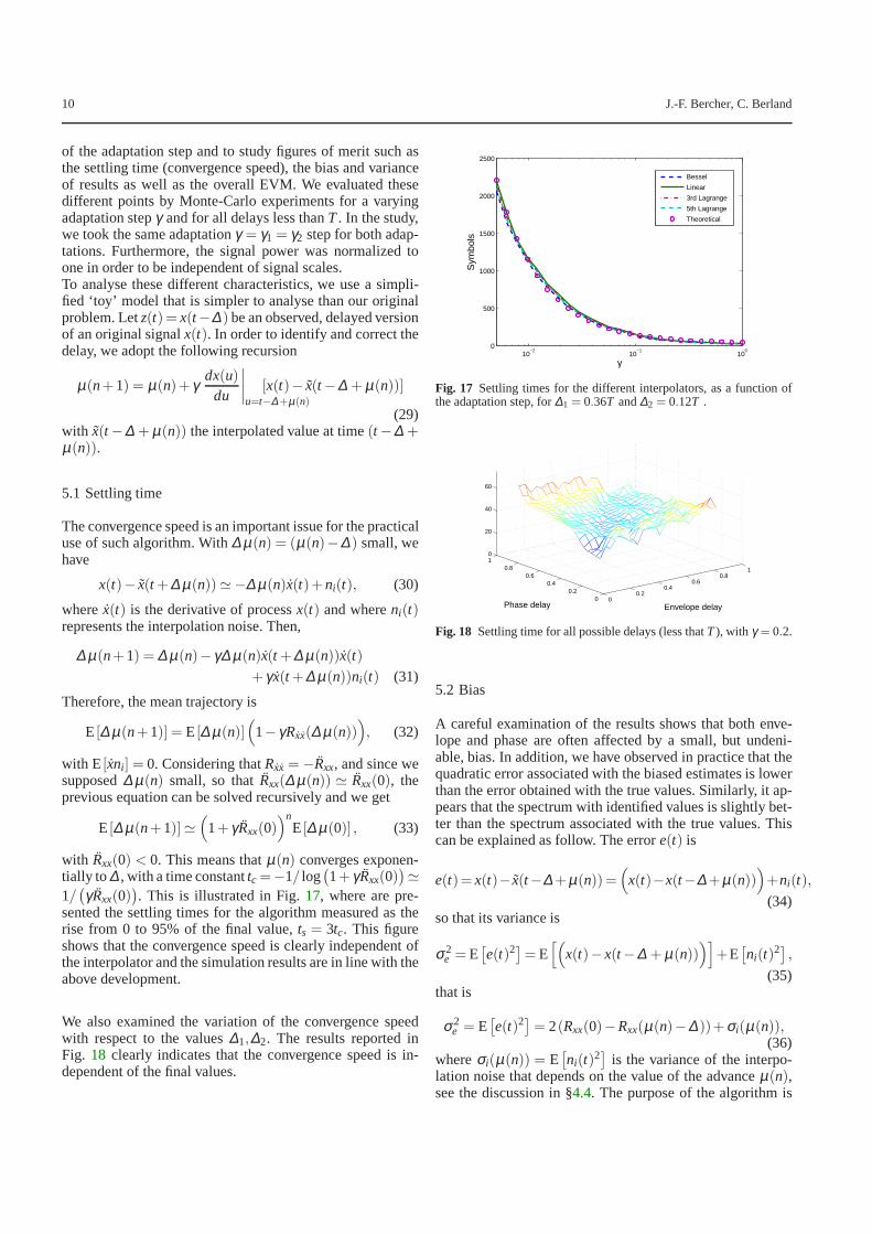
. This is illustrated in Fig.17, where are pre-sented the settling times for the algorithm measured as therise from 0 to 95% of the final value,ts = 3tc. This figureshows that the convergence speed is clearly independent ofthe interpolator and the simulation results are in line withtheabove development.

We also examined the variation of the convergence speedwith respect to the values∆1,∆2. The results reported inFig. 18 clearly indicates that the convergence speed is in-dependent of the final values.

10−2

10−1

100

0

500

1000

1500

2000

2500

γ

Sym

bols

Bessel

Linear

3rd Lagrange

5th Lagrange

Theoretical

Fig. 17 Settling times for the different interpolators, as a function ofthe adaptation step, for∆1 = 0.36T and∆2 = 0.12T .

00.2

0.40.6

0.81

00.2

0.40.6

0.810

20

40

60

Envelope delayPhase delay

Fig. 18 Settling time for all possible delays (less thatT), with γ = 0.2.

5.2 Bias

A careful examination of the results shows that both enve-lope and phase are often affected by a small, but undeni-able, bias. In addition, we have observed in practice that thequadratic error associated with the biased estimates is lowerthan the error obtained with the true values. Similarly, it ap-pears that the spectrum with identified values is slightly bet-ter than the spectrum associated with the true values. Thiscan be explained as follow. The errore(t) is

e(t)= x(t)− x(t−∆ +µ(n))=(

x(t)−x(t−∆ +µ(n)))

+ni(t),

(34)so that its variance is

σ2e = E

[

e(t)2]= E[(

x(t)−x(t−∆ + µ(n)))]

+E[

ni(t)2] ,

(35)that is

σ2e = E

[

e(t)2]= 2(Rxx(0)−Rxx(µ(n)−∆ ))+σi(µ(n)),(36)

whereσi(µ(n)) = E[

ni(t)2]

is the variance of the interpo-lation noise that depends on the value of the advanceµ(n),see the discussion in §4.4. The purpose of the algorithm is

Envelope and Phase delays correction in an EER radio architecture 11

to find a valueµ minimizing σ2e . The first term clearly de-

creases whenµ(n)→∆ while the second term may increase.Therefore, the procedure will find the best values that mini-mize the sum of the two terms, realizing a trade-off betweenbias and variance of the interpolation noise. The solution istheoretically given by

Rxx(µ(n)−∆ ) = −dσ2i (µ(n))

dµ(n). (37)

Fig.19presents the bias measured for the envelope and phasecomponent with respect to the adaptation parameter. We findthat the bias still exist and do not depend on the adaptationparameterγ as it was indicated by the analysis. The bias is afunction of the interpolator type and order.

0.1 0.2 0.3 0.4 0.5 0.6 0.7 0.8 0.9 1−0.03

−0.025

−0.02

−0.015

−0.01

−0.005

0

0.005

0.01

0.015

γ

Bessel

Linear

3rd Lagrange

5th Lagrange

Fig. 19 Biasµ −∆ for the different interpolators, as a function of theadaptation parameterγ . Phase (indicated by−◦−) and envelope biasare almost constant with respect toγ .

5.3 Variance

Variations after convergence are also an important issue. Thesevariations can be modeled as an additive noise on the esti-mates. With our toy model, we obtained expression (31) forthe trajectory of the algorithm. This expression is only valid,on average, if∆ µ(n+1) has a zero mean. Thus, taking now∆ µ(n+ 1) = µ(n+ 1)− µ , whereµ is the value at conver-gence and rearranging the terms, we get

∆ µ(n+1) = ∆ µ(n)(

1− γ x(t +∆ µ(n))x(t))

+ γ x(t +∆ µ(n))ni(t). = An∆ µ(n)+Bnni(t) (38)

Taking the square and the expectation and making the, clearlyfalse, hypothesis thatAn and∆ µ(n), Bn andni(t) are uncor-related, we obtain

σ2µ(n+1) = E

[

A2n

]

σ2µ(n)+E

[

B2n

]

σ2i (39)

with σ2µ(n) the variance ofµ at stepn. We also find E

[

A2n

]

≃1+ 2γRxx(0)+ γ2E

[

x(t)4]

(with µ −∆ ≃ 0), and E[

B2n

]

=

−γ2Rxx(0). At convergence, we finally obtain

σ2µ =

E[

B2n

]

σ2i

1−E[A2n]

=γσ2

i

2+ γE[x(t)4]/Rxx(0). (40)

This expression shows that the variance of the estimates in-creases linearly withγ and that it is only associated to the‘self-noise’ in the system. Despite using approximations inthe derivation, the simulation results are once more in linewith this formula. Fig.20gives the variance of the estimatesof the envelope and phase delays as a function ofγ . The lin-ear dependence can be clearly seen.

0 0.1 0.2 0.3 0.4 0.5 0.6 0.7 0.8 0.9 10

0.5

1

1.5

2

2.5x 10

−3

γ

Bessel

Linear

3rd Lagrange

5 th Lagrange

Fig. 20 Varianceσ 2µ of delays estimates,∆1 = 0.36T,∆2 = 0.12T, for

the different interpolators, as a function of the adaptation parameterγ .Phase (indicated by−◦−) and envelope variances increase linearlywith γ .

5.4 EVM - Quadratic error

The EVM is a crucial parameter in digital communications.As we will observe, it sums up some of the other proper-ties. In the case of a single carrier modulation, the EVM isdefined by E

[

|Ze−Zo|2]

/E[

|Zo|2]

whereZe = ρeejφe andZo = ρoejφo stand for the complex envelope of the emit-ted signal and the original signal respectively. Let us insiston the fact that the situation is more complicated for multi-carrier modulations. In our setting, the expression becomes

EVM =E[

ρ2o +ρ2

e −2ρoρecos(φo−φe)]

E[ρ2o ]

. (41)

Therefore, if∆φ = φo − φe is small, cos∆φ ≃ 1−∆φ2/2,the expression becomes

EVM =E[

(ρo−ρe)2 +ρoρe∆φ2

]

E[ρ2o ]

≃ E[

∆ρ2 +ρ2o∆φ2

]

E[ρ2o ]

(42)or

EVM ≃ E[

∆ρ2]

E[ρ2o ]

+E[

∆φ2] (43)

assuming thatρo and∆φ are independent. As a result, theEVM is a function of the quantities we previously studied.

12 J.-F. Bercher, C. Berland

We already established that the estimates are biased and thattheir variances, which are proportional to interpolation noise,increase linearly withγ . Therefore, the EVM behaves as

EVM ≃ γ2

[

σ2ρ

E[ρ2o ]

+σ2φ

]

+

[

B2ρ

E[ρ2o ]

+B2φ

]

, (44)

whereσ2ρ andσ2

φ are the variances of interpolation noise forthe envelope and phase, andBρ andBφ the bias terms. Since√

1+αx≃ 1+αx/2, the EVM rms may also show the samebehaviour. This is the case in Fig.21 where we clearly seea linear slope and an offset value. It also shows that the La-grange and Bessel interpolators have the best performances.

0 0.1 0.2 0.3 0.4 0.5 0.6 0.7 0.8 0.9 10.5

1

1.5

2

2.5

γ

Bessel

Linear

3rd Lagrange

5th Lagrange

Fig. 21 EVM rms (in %) at the output of the algorithm, for delays∆1 = 0.36T,∆2 = 0.12T as a function of the adaptation parameterγ .

It is also interesting to look at the EVM with respect to allpossible delays and with a fixedγ . Fig. 22 presents theseresults forγ = 0.05. We can observe a ‘modulation’ whichis related to the variable variance of the interpolation noisewith respect to the delay (see Fig.14). Here, as in previousexamples, we tookT/Ts= 5 and indeed notice error minimaat interpolation nodes.

0

0.2

0.4

0.6

0.8

1

0

0.2

0.4

0.6

0.8

10

0.5

1

1.5

Envelope delayPhase delay

Fig. 22 EVM at output of the algorithm withγ = 0.05, for all possibledelays. The ‘modulation’ is related to the non-stationary interpolationnoise that vanishes at interpolation nodes.

Table 3 Settling times of the algorithm and EVM rms (in %) for theoutput, for different interpolators and several values of the adaptationstepγ .

Settling time EVM rms %γ 3rd Lag Bessel 5th Lag

0.05 228 1.045 0.89 0.8150.1 127 1.07 0.9 0.840.5 45 1.24 1.05 1.009

5.5 Summary of the results

In the previous developments we have examined the behaviourof our algorithm according to the choice of interpolators andadaptation steps. Using specific examples, we have demon-strated a vast improvement can be achieved in terms of EVMand output spectrum, as shown in figures15and16. Further-more, using an approximate ‘toy’ model of the algorithm, wehave shown theoretically and checked numerically, that

– the settling time decreases exponentially with the adap-tation step (Fig.17),

– a small estimation bias exists that does not depend onthe adaptation parameter but rather of interpolation order(Fig. 19). The presence of this bias is explained as a wayto reduce the whole quadratic error,

– the variance (40) behaves approximately as a linear func-tion of the adaptation parameter (Fig.20),

– the EVM (44) increases linearly with the adaptation stepγ (Fig. 21).

As a consequence, a trade-off has to be made between thetwo important parameters that are the settling time and theEVM. The choice of the order of the interpolation is alsoimportant with respect to performances and implementationcosts. The main values for the bias and variance can be foundin Table 2 for different interpolators and several values ofthe adaptation stepγ . The results for the settling time andthe EVM are reported in Table 3 for the same conditions.In order to ensure independence in signal scales, the signalpower was normalized to one.

6 Conclusion

In this paper, we proposed and analysed a new synchro-nization algorithm tailored for an EER architecture. Perfor-mances are indeed severely degraded in case of delay mis-match between envelope and phase paths. The proposed al-gorithm is based on an adaptive LMS structure. We studiedthe influence of the adaptation on the quadratic error, EVMand output spectrum. The algorithm uses an interpolationprocedure that is characterized in terms of performances andin terms of implementation. We also examined the influenceof the sampling rate. These studies demonstrated the stronginterest of such a mandatory correction algorithm and theenhancement of transmitter performances.

Envelope and Phase delays correction in an EER radio architecture 13

Table 2 Bias(µ −∆) and varianceσ 2µ of the estimates of delays, for different interpolators andseveral values of the adaptation stepγ .

Bias×103 Variance×105

γ 3rd Lag Bessel 5th Lag 3rd Lag Bessel 5th Lag0.05 ρ -15.5 8 -9 6.2 10 5.80.05 φ -19 2 -9 5.8 6.59 5.750.1 ρ -15 8 -8 11.5 21 11.50.1 φ -28 4 -8 4.5 4.6 4.50.5 ρ -14 8 -7 56.5 89 560.5 φ -17 4 -9 13 11.5 11.5

Regarding the algorithm, a few points can be further investi-gated: adopting different adaptation steps for the two recur-sions, decrasing the number of adaptation steps and alternat-ing the two recursions. Higher system view point has to betaken into account in order to define the best use of the pro-cedure: full tracking of delays or training periods. A for theimplementation, modified and optimized Farrow structuresshould be considered.

This solution has drawbacks. For instance, it requires I/Q de-modulation and uses a Cordic processor to split the envelopeand phase of the PA output signal (derivative computation).We are currently working on these issues to improve our sys-tem.

Other concerns are the behaviour of the system with furthermismatches such as a complex gain in the feedback loop,non-linear distortions and quantization noise. Preliminaryresults show that the algorithm is robust against the gainand noise mismatch, in the sense that the optimum solutionremains unchanged. Evidently further mismatches imply adegradation of performances so future work will include at-tempts to also correct these mismatches with the same feed-back loop.

Acknowledgements The authors are indebted to the anonymous ref-erees for their careful reading of the manuscript as well as their valu-able comments and suggestions that helped improve the presentation ofthis paper. Thanks are extended to S. Trudel, P. J. Duriez andL. Garbellfor their invaluable and friendly proofreading of the manuscript.

References

1. Abramowitz M, Stegun IA (1965) Handbook of MathematicalFunctions: with Formulas, Graphs, and Mathematical Tables.Dover Publications

2. Baudoin G, Berland C, Villegas M, Diet A (2003) Influence oftime and processing mismatches between phase and envelopesignals in linearization systems using envelope elimination andrestoration, application to hiperlan2. In: Microwave SymposiumDigest, 2003 IEEE MTT-S International, vol 3, pp 2149–2152

3. Bercher JF, Berland C (2006) Envelope/phase delays correctionin an EER radio architecture. In: Proceedings of the 13th IEEEInternational Conference on Electronics, Circuits, and Systems,ICECS2006, pp 443–446

4. Bercher JF, Diet A, Berland C, Baudoin G, Villegas M (2004)Monte-carlo estimation of time mismatch effect in an OFDM EER

architecture. In: Proceedings of the 2004 IEEE Radio and WirelessConference, pp 283–286

5. Candan C (2007) An efficient filtering structure for Lagrange in-terpolation. IEEE Signal Processing Letters 14:17–19

6. Crochiere R, Rabiner L (1975) Optimum fir digital filter imple-mentations for decimation, interpolation, and narrow-band filter-ing. IEEE Transactions on Acoustics, Speech, and Signal Process-ing 23(5):444–456

7. Dempster A, Murphy N (2000) Efficient interpolators and filterbanks using multiplier blocks. IEEE Transactions on SignalPro-cessing 48:257–261

8. Farrow CW (1988) A continuous variable digital delay element.In: Proc. IEEE Int. Symp. Circuits Systems, pp 2641–2645

9. Hentschel T (2002) Sample Rate Conversion in Software Config-urable Radios. Artech House Publishers

10. Hentschel T, Fettweis G (2002) The Digital Front-End – BridgeBetween RF-and Baseband-Processing. In: Software Defined Ra-dio Enabling Technologies, John Wiley & Sons Ltd, pp 151–198

11. Jau JK, Horng TS (2001) Linear interpolation scheme for com-pensation of path delay difference in an envelope elimination andrestoration transmitter. In: Proceedings of Asia-Pacific MicrowaveConference, 2001. APMC 2001, vol 3, pp 1072–1075 vol.3

12. Johansson H, Gustafsson O (2005) Linear-phase FIR interpola-tion, decimation, andmth-band filters utilizing the Farrow struc-ture. IEEE Transactions on Circuits and Systems I 52:2197–2207

13. Johansson H, Lowenborg P (2003) On the design of adjustablefractional delay FIR filters. IEEE Transactions on CircuitsandSystems II 50:164–169

14. Kahn L (1952) Single-sideband transmission by envelopeelimi-nation and restoration. Proceedings of the IRE 40(7):803–806

15. Laakso TI, Valimaki V, Karjalainen M, Laine UK (1996) Splittingthe unit delay. IEEE Signal Processing Magazine 13:30–60

16. Makundi M, Laakso T, Valimaki V (2001) Efficient tunable IIRand allpass filter structures. Electronics Letters 37:344–345

17. Mártires J, Borg C, Larsen T (2006) Differential delay equaliza-tion in a Kahn EER transmitter. In: ST Mobile & Wireless Com-munications Summit, nr. 15th, Myconos, Grækenland

18. Morgan P (2006) Highly integrated transceiver enables high-volume production of GSM/EDGE handsets. RFdesign pp 36–42

19. Oetken G (1979) A new approach for the design of digital interpo-lating filters. IEEE Transactions on Acoustics, Speech, andSignalProcessing 27(6):637–643

20. Raab F (1977) Idealized operation of the class e tuned power am-plifier. Circuits and Systems, IEEE Transactions on 24:725–735

21. Sander WB, Schell SV, Sander BL (2003) Polar modulator formulti-mode cell phones. Proceedings of the IEEE 2003 CustomIntegrated Circuits Conference pp 439–445

22. Sarigeorgidis K, Rabaey J (2004) Ultra low power cordic proces-sor for wireless communication algorithms. Journal of VLSISig-nal processing 38:115–130

23. Staszewski R, Wallberg J, Rezeq S, Hung CM, Eliezer O, Vem-ulapalli S, Fernando C, Maggio K, Staszewski R, Barton N, LeeMC, Cruise P, Entezari M, Muhammad K, Leipold D (2005) All-digital PLL and transmitter for mobile phones. IEEE JournalofSolid-State Circuits 40(12):2469–2482

24. Strasser G, Lindner B, Maurer L, Hueber G, Springer A (2006) Onthe spectral regrowth in polar transmitters. In: MicrowaveSympo-

14 J.-F. Bercher, C. Berland

sium Digest, 2006. IEEE MTT-S International, pp 781–78425. Valimaki V (1995) A new filter implementation strategy for La-

grange interpolation. In: Proceedings of the 1995 IEEE Interna-tional Symposium on Circuits and Systems, ISCAS ’95, vol 1, pp361–364 vol.1

26. Valimaki V, Laakso TI (2000) Principles of fractional delay fil-ters. Proceedings of IEEE International Conference on Acoustics,Speech, and Signal Processing, ICASSP’00 6

27. Vesma J, Saramaki T (1997) Optimization and efficient implemen-tation of FIR filters with adjustable fractional delay. In: Proceed-ings of 1997 IEEE International Symposium on Circuits and Sys-tems, ISCAS ’97, vol 4, pp 2256–2259 vol.4

28. Volkov EA (1986) Numerical Methods. Mir Publisher Moscow29. Whittaker JM (1935) Interpolatory Function Theory. Cambridge

Univ. Press, Cambridge, England30. Yli-Kaakinen, Saramaki (2006) Multiplication-free polynomial-

based FIR filters with an adjustable fractional delay. Circuits, Sys-tems, and Signal Processing 25:265–294

31. Yli-Kaakinen J, Saramaki T (2004) An algorithm for the optimiza-tion of adjustable fractional-delay all-pass filters. In: Proceedingsof the 2004 International Symposium on Circuits and SystemsIS-CAS’04, vol 3, pp III–153–6 Vol.3

32. Yli-Kaakinen J, Saramaki T (2007) A simplified structurefor FIRfilters with an adjustable fractional delay. IEEE International Sym-posium on Circuits and Systems, 2007 ISCAS 2007 pp 3439–3442