Soliton staircases and standing strain waves in confined colloidal crystals

arX
iv:p
hysi
cs/0
2040
50v2
[ph
ysic
s.pl
asm
-ph]
29
May
200
2
Soliton self-modulation of the turbulence
amplitude and plasma rotation
Florin Spineanu and Madalina Vlad
Association Euratom-C.E.A. sur la Fusion, C.E.A.-Cadarache,
F-13108 Saint-Paul-lez-Durance, France
and
Association Euratom-NASTI Romania,
National Institute for Laser, Plasma and Radiation Physics,
P.O.Box MG-36, Magurele, Bucharest, Romania
E-mails: [email protected], [email protected]
February 2, 2008
Abstract
The space-uniform amplitude envelope of the Ion Temperature Gra-
dient driven turbulence is unstable to small perturbations and evolves to
nonuniform, soliton-like modulated profiles. The induced poloidal asym-
metry of the transport fluxes can generate spontaneous poloidal spin-up
of the tokamak plasma.
Contents
1 Introduction 2
2 The slab model of the ion mode instability 32.1 The mode evolution in a fixed plasma rotation profile . . . . . . 8
2.2 Nondimensional form of the equation . . . . . . . . . . . . . . . . 10
3 Multiple time and space scale analysis of the ion mode equationreduced to the barotropic form 123.1 The enveloppe equation . . . . . . . . . . . . . . . . . . . . . . . 143.2 Numerical search for classes of admissible envelope solutions . . . 27
4 Exact solutions of the Nonlinear Schrodinger Equation and thenonlinear stability problem 274.1 Introduction . . . . . . . . . . . . . . . . . . . . . . . . . . . . . . 274.2 The Lax operators and the main spectrum . . . . . . . . . . . . . 30
1

4.3 Solving the eigenvalue equation for the operator L . . . . . . . . 314.4 The “squared” eigenfunctions . . . . . . . . . . . . . . . . . . . . 34
4.4.1 The two Bloch functions for the operator L . . . . . . . . 344.4.2 Product expansion of g and its zeros µj (x, t). Introduc-
tion of the hyperelliptic functions µj . . . . . . . . . . . . 364.5 Solution: the two-sheeted Riemann surface (hyperelliptic genus-
N Riemann surface) . . . . . . . . . . . . . . . . . . . . . . . . . 384.5.1 Holomorphic differential forms and cycles on the Riemann
surface . . . . . . . . . . . . . . . . . . . . . . . . . . . . . 384.5.2 Periods and matrices of periods . . . . . . . . . . . . . . . 394.5.3 The Abel map . . . . . . . . . . . . . . . . . . . . . . . . 404.5.4 The Jacobi inversion problem . . . . . . . . . . . . . . . . 42
5 Stability of the envelope solutions 455.1 Modulation instability of the envelope of a plane wave . . . . . . 46
5.1.1 General method . . . . . . . . . . . . . . . . . . . . . . . 465.1.2 Calculation of the main spectrum associated to the uni-
form amplitude solution . . . . . . . . . . . . . . . . . . . 475.2 The spectrum of the plane wave solution . . . . . . . . . . . . . . 48
5.2.1 The spectrum of the unperturbed initial condition (caseof plane wave) . . . . . . . . . . . . . . . . . . . . . . . . 48
5.2.2 The spectrum of the perturbed initial condition (case ofplane wave) . . . . . . . . . . . . . . . . . . . . . . . . . . 51
6 The growth of the perturbed solution as a source of poloidalasymmetry and spontaneous plasma spin-up 556.1 The minimal condition for instability of the poloidal rotation . . 556.2 The soliton developing from the initial perturbation . . . . . . . 566.3 The poloidal asymmetry of the diffusion fluxes . . . . . . . . . . 576.4 The poloidal torque applied on plasma . . . . . . . . . . . . . . . 61
7 Discussion 64
1 Introduction
The ion temperature gradient turbulence, considered a major source of anoma-lous transport in the tokamak plasma, is characterized by the coexistence ofirregular patterns (randomly fluctuating field) and intermittent robust cuasi-coherent structures. In closely related fluid models (for exemple, in the physicsof atmosphere) modulational instabilities are known to produce solitary struc-tures on the envelope of the fluctuating field. In the case of the tokamak, thiscan be particularly important since a poloidally nonuniform amplitude of theturbulence generates nonuniform transport rates. For a sufficiently high nonuni-formity the torque arising via the mechanism initially mentioned by Stringer [1]may overcame the rotation damping due to the poloidal magnetic pumping. In
2

this work we show that this can indeed be the case by proving that the uni-form poloidal envelope of the ITG turbulence is an unstable state. It appearsthat the ITG turbulence has intrinsic resources to generate poloidal rotationvia a combination of mechanisms which is not directly related to the Reynoldsstress, inverse cascade, direct-ion loss, or other classical sources of rotation. Weprovide an essentially mathematical explanation of the instability of the solu-tion consisting of poloidally uniform envelope of the turbulence. Based on thegeometrico-algebraic method of solving integrable nonlinear differential equa-tions on periodic domains we invoke an existing result, that any perturbationremoves the degeneracies due to coincident eigenvalues in the main spectrum ofthe Lax operator, thus changing the topology of the hyperelliptic Riemann sur-face that provides the solution. The perturbed solution separates exponentially(in function space) from the initial one (uniform envelope) and this yields anexponential growth of the poloidal nonuniformity. The magnitude of the torquemay be comparable to the poloidal magnetic damping.
There are many works in plasma physics related to the soliton dynamics [2],[3], [4], [5], [7], etc. In a recent paper the focusing solution has been used to studythe formation of coherent motion or intermittent patterns (streamers) [2]. Ourwork is basically a mathematical approach, using well developed technics relatedto the Inverse Scattering Transform method for periodic domains. However,more physical analysis may become possible combining the knowledge of thespectral properties of the ion turbulence with the nonlinear stability properties.
This work consists of several parts that may appear as developing separately:the derivation of the ion equation (barotropic equation), the multiple space-time scales analysis, the solution of the Nonlinear Schrodinger Equation andthe stability of the solution, the torque arising from the Stringer mechanismand the possibility of the rotation. For being self-contained the paper alsoincludes a review of the multiple space-time analysis (from the atmosphericphysics applications) and of the geometric-algebraic method of integration ofthe Nonlinear Schrodinger Equation. Even if these parts could be found in basicworks (see the references) they are included both for clarity and for their extremeimportance for further applications related to our problem or independent ofthis.
2 The slab model of the ion mode instability
We consider cylindrical geometry with circular magnetic surfaces. Locally themodel can be reduced to a slab geometry with (x, y) cartezian coordinates re-placing respectively the radius and poloidal angle coordinates (r, θ). At equilib-rium the plasma parameters are constant on the magnetic surfaces. The effectsof the toroidicity and of the particle drifts are not included instead the nonlin-earity related to the ion polarization drift is fully retained. The plasma modelconsists of the continuity equations and the equations of motion for electrons
3

and ions:
∂nα
∂t+ ∇· (nαvα) = 0 (1)
mαnα
(∂vα
∂t+ (vα · ∇)vα
)= −∇pα − ∇ · πα + eαnα (E + vα×B) + Rα
(2)
where α = e, i. The friction forces Re = −Ri = −n |e|J‖/σ‖ , which are im-portant for the parallel electron momentum balance, vanish for infinite plasmaconductivity, which we will assume. The collisional viscosity πe,i will be ne-glected as well. However we will need to include it later when we will considerthe balance of the forces contributing to the poloidal rotation. The electron andion temperatures are considered constant along the magnetic lines ∇‖Te,i = 0.The equilibrium quantities are perturbed by the wave potential φ: n = n0 + n.A sheared poloidal plasma rotation is included, and we later will make explicitthe corresponding part in the potential, φ0.
The momentum conservation equations are used to determine the perpendic-ular velocities of the electrons and ions. The parallel momentum conservationequation for electrons, in the absence of dissipation or drifts gives the adiabaticdistribution of the density fluctuation. The velocities are introduced in the con-tinuity equations to find the dynamical equations for the density and electricpotential.
From the equations of motion for the ions the velocities are obtained in theform:
vi = v⊥i = vdia,i + vE + vpol,i
where the ion diamagnetic velocity is
vdia,i =1
ni
1
miΩin × ∇pi
The versor of the magnetic field is n; the versors along the transversal coordinateaxis (x, y) will be noted (ex, ey). The ion-polarization velocity is:
vpol,i = − 1
|e|niBnimi
(∂vE
∂t+ (vE · ∇)vE
)× n (3)
= − 1
BΩi
(∂
∂t+ (vE · ∇⊥)
)∇⊥φ
Using the notation ddt ≡ ∂
∂t + (vE · ∇⊥) the perpendicular ion velocity can bewritten
v⊥,i = vdia,i + vpol,i +−∇φ× n
B(4)
=Ti
|e|B1
ni
dni
drey − 1
BΩi
d
dt(∇⊥φ) +
−∇φ× n
B
4

The equation for the velocity of the electrons is
ve = v⊥,e + v‖,e
v⊥e = vE + vdia,e (5)
=−∇φ× n
B+
1
n
1
meΩe(n× ∇p)
=−∇φ× n
B+
Te
− |e|B1
n0
dn0
drey (6)
We assume neutrality ne = ni = n and introduce the expressions of thevelocities in the continuity equations for ions and for electrons.
The ion continuity equation is
∂n
∂t+ ∇· (nv⊥,i) = 0
The electron continuity equation is
∂n
∂t+ ∇⊥· (nv⊥,e) + ∇‖
(nv‖e
)= 0
The equations are substracted , to obtain
−∇‖
(nv‖e
)
− 1
BΩi∇⊥ ·
(nd
dt∇⊥φ
)
+∇⊥ · (nvdia,i) − ∇⊥ · (nvdia,e)
= 0
From the last term in the left we get:
dn0
dxex · vdia,i + (∇⊥n) · vdia,i =
= −Ti
Te
(Te
|e|B1
n0
dn0
dx
)∂n
∂y
Including the similar term for the electrons, we obtain
−∇‖
(nv‖e
)
− 1
BΩi∇⊥ ·
(nd
dt∇⊥φ
)
−Ti
Te
(Te
|e|B1
n0
dn0
dx
)∂n
∂y−(
Te
|e|B1
n0
dn0
dx
)∂n
∂y
= 0
5
or:
−(
1 +Ti
Te
)(Te
|e|B1
n0
dn0
dx
)∂n
∂y+
1
BΩi∇⊥ ·
(nd
dt∇⊥φ
)+ ∇‖
(nv‖e
)= 0
(7)
From the continuity equation for electrons
∂n
∂t+ ∇⊥ · (nv⊥) + ∇‖ ·
(nv‖
)= 0 (8)
we obtain
∂n
∂t+
1
B
∂φ
∂y
dn0
dx+ +vdia,e · ∇⊥n+ V0
∂n
∂y+ (9)
+n0
(∇‖ · v‖
)+ v‖∇‖n
= 0
where the seed poloidal velocity is V0 (x) = − dφ0(x)Bdx ey. The parallel moment-
tum balance gives the parallel electron velocity
v‖e = −σ‖
e2∇‖ (|e|φ+ Te ln (n/n0)) (10)
In the absence of friction (σ → ∞) and of particle drifts the electron responseis adiabatic
n
n0= −|e|φ
Te
and the potential is determined from Eq.(7). To develop separately the ion-polarization drift term, we introduce the notation:
W ≡ 1
BΩi∇⊥·
[(n0 + n)
(∂
∂t+ vE · ∇⊥
)∇⊥φ
]
=1
BΩi∇⊥· [(n0 + n) I]
where we make explicit the electric potential φ0 associated to the initial plasmapoloidal rotation, V0ey.
I ≡(∂
∂t+ (V0ey + v) · ∇⊥
)∇⊥
(φ0 + φ
)
We have
I =∂
∂t(∇⊥φ0) +
+∂
∂t
(∇⊥φ
)+
+
[V0
∂
∂y+ (v · ∇⊥)
] (∇⊥φ0 + ∇⊥φ
)
6

or
I =∂
∂t(exBV0) +
+∂
∂t
(∇⊥φ
)+
+
[V0
∂
∂y+ (v · ∇⊥)
] (∇⊥φ0 + ∇⊥φ
)
=∂
∂t(exBV0) + V0B
∂V0
∂yex +
+∂
∂t
(∇⊥φ
)+ (v · ∇⊥)BV0ex +
+V0∂
∂y
(∇⊥φ
)+ (v · ∇⊥)
(∇⊥φ
)
with the relations
∇⊥φ = B (v × n)
= (Bvy) ex + (−Bvx) ey
vy =1
B
∂φ
∂xand vx = − 1
B
∂φ
∂y
After very simple calculations we obtain:
1
BIx =
∂V0
∂t+ vy
∂V0
∂y+ V0
∂V0
∂y(11)
+∂vy
∂t+ vx
∂V0
∂x+ V0
∂vy
∂y
+vx∂vy
∂x+ vy
∂vy
∂y
and
1
BIy = −∂vx
∂t− V0
∂vx
∂y(12)
−vx∂vx
∂x− vy
∂vx
∂y
7

It will be useful to calculate the derivaties of these quantities
1
B
∂Ix∂x
=∂
∂x
∂V0
∂t+∂vy
∂x
∂V0
∂y+ vy
∂2V0
∂y∂x+∂V0
∂x
∂V0
∂y+ V0
∂2V0
∂x∂y(13)
+∂vy
∂t
∂V0
∂x+ vx
∂2V0
∂x2+∂
∂t
∂vy
∂x+
+∂V0
∂x
∂vy
∂y+ V0
∂2vy
∂x∂y+
+∂vx
∂x
∂vx
∂y+ vx
∂2vy
∂x2+
+∂vy
∂x
∂vy
∂y+ vy
∂2vy
∂x∂y
and
1
B
∂Iy∂y
= −∂V0
∂y
∂vx
∂y(14)
− ∂
∂t
∂vx
∂y− V0
∂2vy
∂y2−
−∂vx
∂y
∂vx
∂x− vx
∂2vx
∂x∂y−
−∂vy
∂y
∂vx
∂y− vy
∂2vx
∂y2
The quantity denoted by W takes the form
W =1
BΩi
(dn0
dx
)Ix +
1
BΩin0
(∂Ix∂x
)+
+1
BΩi
(∂n
∂x
)Ix +
1
BΩin
(∂Ix∂x
)+
+1
BΩin0
(∂Iy∂y
)+
1
BΩi
(∂n
∂y
)Iy +
1
BΩin
(∂Iy∂y
)
2.1 The mode evolution in a fixed plasma rotation profile
We will assume that the mode evolves initially without perturbing the equilib-rium profiles, in particular the seed poloidal rotation. This allows us to simplifythe expressions above, taking:
∂V0
∂y= 0
∂V0
∂t= 0
8

Then the first lines in the formulas Eqs.(11), (13), (14) are zero. Let us considerin the expression of W the part W0 which does not contain the fluctuatingdensity n. Writting
W = W0 + W
we have
W0 ≡ 1
Ωi
(dn0
dx
)[vx∂V0
∂x+ V0
∂vy
∂y+ vx
∂vy
∂x+ vy
∂vy
∂y+∂vy
∂t
]+
+1
Ωin0∇⊥ · (Ixex + Iy ey)
and
W =1
BΩi
(∂n
∂x
)Ix +
1
BΩin
(∂Ix∂x
)+
1
BΩi
(∂n
∂y
)Iy +
1
BΩin
(∂Iy∂y
)
Replacing the perturbed velocity by the perturbed potential, writting all termsand summing, we get:
W0 =
(∂
∂t+ V0
∂
∂y
)1
B
∂φ
∂x+
(− 1
B
∂φ
∂y
)dV0
dx+
(−∇⊥φ× n
B· ∇⊥
)∂φ
∂x+
+1
Ωin0
1
BV0
∂
∂y∇2
⊥φ+
+1
B
(−∇⊥φ× n
B· ∇⊥
)∇2
⊥φ−
− 1
B
∂φ
∂y
d2V0
dx2+
+1
B
∂
∂t
(∇2
⊥φ)
Collecting all what we have at this moment the ion continuity equation (7)becomes:
∇‖
(nv‖e
)+
−(
1 +Ti
Te
)(Te
|e|B1
n0
dn0
dx
)∂n
∂y+
+1
BΩin0
(∂
∂t+ V0
∂
∂y
)∇2
⊥φ− V′′
0
∂φ
∂y+
(−∇⊥φ× n
B· ∇⊥
)∇2
⊥φ
+1
BΩi
(dn0
dx
)[(∂
∂t+ V0
∂
∂y
)vy + vx
∂vy
∂x+ vy
∂vy
∂y+ vx
∂V0
∂x
]
+W + terms of the first line in the expressions of Ix and derivatives= 0
In the above equation (which is exact) we shall make the following approxi-mations:
9

• neglect the term containing the parallel electron velocity, assuming infiniteelectric conductivity;
• neglect the term which contains dn0/dx since it is in the ratio k : 1/Ln
with the other terms, and we consider
kLn ≪ 1
• neglect W ; these terms are in the ratio n/n0 with the terms which areretained;
• neglect of the terms in the first lines of the expressions for Ix and dIx/dx,dIy/dy. (These are the terms in the curly brakets, the last line). Asexplained above, we assume that the mode evolves in a background offixed rotation profile, V0 (x).
The resulting equation is
−BΩi
(1 +
Ti
Te
)(Te
|e|B1
n0
dn0
dx
)∂
∂y
(n
n0
)
+
(∂
∂t+ V0
∂
∂y
)∇2
⊥φ− V′′
0
∂φ
∂y+
(−∇⊥φ× n
B· ∇⊥
)∇2
⊥φ
= 0
and, replace the adiabatic form of the density perturbation
n
n0= −|e| φ
Te
We define
β ≡ BΩi
(1 +
Ti
Te
)(Te
|e|B1
n0
dn0
dx
) |e|Te
= Ωi
(1 +
Ti
Te
)1
Ln
and obtain
β∂φ
∂y+
(∂
∂t+ V0
∂
∂y
)∇2
⊥φ− V′′
0
∂φ
∂y+
(−∇⊥φ× n
B· ∇⊥
)∇2
⊥φ = 0
which is the barotropic equation.
2.2 Nondimensional form of the equation
We consider that the ion mode extends in the spatial (x) direction over a lengthL. A typical value for the sheared poloidal rotation is noted U0. We make thereplacements
y → Ly
10

t→ tL
U0
φ→ φTe
|e|
V0 → UU0
such that from now on y, t, φ and U are nondimensional quantities. We alsochange the radial coordinate into a dimensionless variable
x→ Lx
and rewrite the equation(
Ωi
(1 +
Ti
Te
)1
Ln
L2
U0
)∂φ
∂y+
+
(∂
∂t+ U
∂
∂y
)∇2
⊥φ
−d2U
dx2
∂φ
∂y+
+
(1
U0
Te
|e|1
B
1
L
)[(−∇⊥φ× n) · ∇⊥]∇2
⊥φ
= 0
The coefficients are
β′ ≡ Ωi
(1 +
Ti
Te
)1
Ln
L2
U0non-dimensional
ε ≡ 1
U0
Te
|e|1
B
1
Lnon-dimensional
For an order of magnitude, ε is the ratio of the diamagnetic electron velocityto the rotation velocity U0 multiplied by the ratio of the density gradient lengthto the length of the spatial domain. This quantity, ε is in general smaller thanunity.
The quantity β′ is the ratio of the ion cyclotron frequency to the inverseof the time required to cross the spatial domain with the typical flow velocity.Since the later (U0/L) involves macroscopic quantities this ratio can be large.It is multiplied by the ratio of the spatial length to the density gradient length(these quantities can be comparable and the ratio not too different of unity).
We change the notations eliminating the primes. The equation becomes
β∂φ
∂y+
(∂
∂t+ U
∂
∂y
)∇2
⊥φ− d2U
dx2
∂φ
∂y+ ε [(−∇⊥φ× n) · ∇⊥]∇2
⊥φ = 0
This is the barotropic equation, known in the physics of the atmosphere.
11

3 Multiple time and space scale analysis of theion mode equation reduced to the barotropic
form
The quasigeostrophic barotropic atmospheric model leads to the barotropicequation (see Horton [7] where the quasigeostrophic approximation is explainedin relation with the Ertel’s theorem). This equation has been studied in theatmosphere science by means of the multiple space and time scales method. Ouraim is similar, i.e. to obtain an equation for the envelope of the fluctuating fieldφ in order to study the possible poloidally nonuniform profiles of the turbulenceaveraged amplitude. The connection between the original equation and the finalslow-time and large-spatial scales equations is not simple : much numerical workis required in order to connect the input physical parameters of the plasmawith the formal coefficients in the final equations. The detailed analytical workis presented in Ref([8]) and the necessary formulas are reproduced here forconvenience. To simplify the expressions the following notation is introduced[φ,∇2φ
]≡ [(−∇⊥φ× n) · ∇⊥]∇2
⊥φ and the equation can be written
(∂
∂t+ U (x)
∂
∂y
)∇2φ+
(β − d2U (x)
dx2
)∂φ
∂y= −ε
[φ,∇2φ
]
The analysis on multiple scales starts by introducing the variables on scalesseparated by the parameter ε:
T1 = εt, T2 = ε2t
Y1 = εy, Y2 = ε2y
This gives for the derivatives
∂
∂t→ ∂
∂t+ ε
∂
∂T1+ ε2
∂
∂T2(15)
∂
∂y→ ∂
∂y+ ε
∂
∂Y1+ ε2
∂
∂Y2(16)
The solution is adopted to be of the form
φ = φ(1) + εφ(2) + ε2φ(3) + · · · (17)
We denote the linear part of the operator in the equation by
L ≡(∂
∂t+ U (x)
∂
∂y
)∇2 +
(β − d2U (x)
dx2
)∂
∂y
12

Substituting the Eq.(17) and the forms of the derivation operators Eqs.(15, 16)in the equation of motion we obtain from the equality between the coefficientsof the powers of the variable ε:
Lφ(1) = 0 (18)
Lφ(2) = (19)
=
(∂
∂T1+ U
∂
∂Y1
)∇2φ(1) + (β − U ′′)
∂φ(1)
∂Y1
−2
(∂
∂t+ U
∂
∂y
)∂2φ(1)
∂y∂Y1
−[φ(1),∇2φ(1)
]
Lφ(3) = (20)
=
(∂
∂T2+ U
∂
∂Y2
)∇2φ(1) − (β − U ′′)
∂φ(1)
∂Y2
−2
(∂
∂t+ U
∂
∂y
)∂2φ(1)
∂y∂Y2
−(∂
∂t+ U
∂
∂y
)∂2φ(1)
∂Y 21
−2
(∂
∂T1+ U
∂
∂Y1
)∂2φ(1)
∂y∂Y1
−(
∂
∂T1+ U
∂
∂Y1
)∇2φ(2)
−2
(∂
∂t+ U
∂
∂y
)∂2φ(2)
∂y∂Y1− (β − U ′′)
∂φ(2)
∂Y1
−∂φ(2)
∂Y1
∂
∂x∇2φ(1) +
∂φ(1)
∂x
∂
∂Y1∇2φ(1)
−2
(∂φ(1)
∂y
∂3φ(1)
∂y∂x∂Y1− ∂φ(1)
∂x
∂3φ(1)
∂y2∂Y1
)
−[φ(1),∇2φ(2)
]−[φ(2),∇2φ(1)
]
The solution is represented on the space and time scales.
13

3.1 The enveloppe equation
The solution of the linear part of the operator, Eq.(18) is adopted as the super-position of two propagating waves
φ(1) = A1 (T1, T2, Y1, Y2)ϕ1 (x) exp (ik1y − iω1t) (21)
+A2 (T1, T2, Y1, Y2)ϕ2 (x) exp (ik2y − iω2t)
+c.c.
The two functions ϕn, n = 1, 2, are solutions of the equation
d2ϕn
dx2−(k2
n − β − U ′′
U − cn
)ϕn = 0 (22)
with
ϕn (0) = ϕn (L) = 0
In this formula, (0, L) are the limits of the spatial domain in the minor radiusdirection where the flow U (x) 6= 0 ; cn = ωn/kn are the phase velocities. Tofind the solutions of this equation we have to use numerical methods. This isa Schrodinger-type equation where the potential depends on the energy, (sincethe phase velocity cn depends on the wavenumber kn). We must use numericalmethods suitable for Sturm-Liouville equations and in general the solution existsfor only particular values of the parameters. We choose to fix the frequencies ωn
and consider kn as the parameter to be determined. The problem is complicatedby the possible occurence of singularities in the potential due to resonancesbetween the phase velocity and the fixed zonal flow. We will avoid any resonancesince the physical content of the processes consisting of the direct energy transferbetween the fluctuations and the flow represents a different physical problemand requires separate consideration. In the present work we examine the effect ofthe turbulence on the poloidal rotation as being due to the nonuniform diffusionrates and Stringer mechanism.
The parameters in the Eqs.(22) are β, ε and the sheared flow velocity U(x).We take for U (x) a symmetric Gaussian-like profile shifted in amplitude andretain its maximum, half-width and asymptotic value (i.e. at x = 0 or L) asparameters. The two frequencies have fixed values during the eigenvalue searchbut they must be considered free parameters as well. This builds up a largespace of parameters which should be sampled. For some point in this space theeigenvalue problems Eqs.(22) are solved and the phase velocities compared withthe profile of U (x). The presence of resonances renders the set of parametersuseless. Since (as will result from the formuals below) there are also otherpossible resonances, the determination of a useful solution (k1, k2) is difficultand requires many trials.
The numerical methods that have been used in solving Eqs.(22) belong to twoclasses: boundary value integration methods and respectively shooting meth-ods. When the sign of the “potential” in the equation is negative everywhere on
14

(0, L) , which occurs for short wavelengths and smooth fluid velocity profile theboundary conditions cannot be fulfilled except for asymtotically, i.e. assumingarbitrary small nonzero values at these limits, since the solution decays expo-nentially. However most of the boundary value integrators we have tried gaveamplitudes of magnitudes comparable to the boundary value, which essentiallyare homotopic to the trivial vanishing solution (the equation is homogeneous)and render useless this approach. We have to use a shooting method acceptingthe difficulty that the initial value of the parameter to be determined (eigen-value) must be placed not far from the final value. We have used the specializedpackage SLEIGN2 interactively. For the investigation of ranges of parametersmost of the calculations have been performed using the routine D02KEF ofNAG. For identical conditions the two numerical codes gave the same resultswithin the accepted tolerance.
Using the routine D02KEF we divide the integration range (0, L) into fourintervals corresponding roughly to a different behaviour of the potential. Thisshould simplify the task of integrator. A single matching point is assumed,usually at the centre. The tolerence is 10−8 which however does not excludefake convergence in case of an initialisation of the eigenvalue very far from thetrue solution..
We notice from Eqs.(22) that the potential can easily be dominated by highshear U ′′ especially for smaller wavenumbers kn. Actually we are more interestedto investigate regimes where only mild effects of the seed sheared rotation ariseduring the process of self-modulation since, as explained before, the possibleevolution to the nonuniformity in the poloidal direction will be the source of thetorque on the plasma. Avoiding regimes of U ′′-dominated potentials we assumelow shear and take the Gaussian profile with Umax − Umin = 2 × 10⁴ (m/s)represented in Figure (1). The following set of physical parameters has beenused: minor radius a = 1 m, magnetic field BT = 3.5 T , electron temperatureTe = 1 KeV , ion temperature Ti = 1 KeV , density n = 1020 m−3, Ln = 10 m.The parameters in the barotropic equation are then: β = 33.526 and ε =0.28571. The two frequencies are ω1 = 85 × 102 s−1 and ω2 = 85 × 104 s−1. Itis assumed that the space region of significant magnitude of U (x) is L = 0.1 m.The following two eigenvalues are obtained, normalised to L−1: k1 = 0.5525and k2 = 3.2029. The potentials in the Schrodinger-like equations and theeigenfunctions are shown in Figure (2).
The two eigenfunctions ϕ1,2 have an important role in the following stepsof the calculation. Substituting the Eq.(21) in the barotropic equation and
15

0 0.2 0.4 0.6 0.8 14
4.5
5
5.5
6Poloidal velocity U(y)
0 0.2 0.4 0.6 0.8 1−15
−10
−5
0
5
10
15First derivative dU(y)/dy
0 0.2 0.4 0.6 0.8 1−200
−150
−100
−50
0
50
100Second derivative d2U(y)/dy2
Figure 1: Profile of the seed sheared poloidal velocity. Also are plotted the firstand the second derivatives.
0 0.5 1−40
−30
−20
−10
0
10
20
−Potential in the Eq. for φ1
0 0.5 1−0.5
0
0.5
1
1.5
The function φ1
0 0.5 1−4
−2
0
2
4
dφ1/dy
0 0.5 1−60
−40
−20
0
20
40
60
−Potential in the Eq. for φ2
0 0.5 1−0.1
0
0.1
0.2
0.3
0.4
0.5
0.6
The function φ2
0 0.5 1−2
−1
0
1
2
dφ2/dy
Figure 2: The potentials in the Schrodinger-type equations and the eigenfunc-tions ϕ1,2. The derivatives of the eigenfunctions are aslo plotted.
16

expanding the operators, we obtain:
Lφ(2) = −2∑
n=1
G1n exp (ikny − iωnt) (23)
−2∑
n=1
ig2nA2n exp [i2 (kny − ωnt)]
−g3A1A2 exp [i (k12y − ω12t)]
−ig4A1A∗2 exp [i (α12y − σ12t)]
+c.c.
where
k12 = k1 + k2
ω12 = ω1 + ω2
We have k12 = 3.755, ω = 8.585.
α12 = k1 − k2
σ12 = ω1 − ω2
or: α12 = −2.650, σ12 = −8.415.
G1n =
(d2ϕn
dx2− k2
nϕn
)∂An
∂T1+
+
[U
(d2ϕn
dx2− k2
nϕn
)+ (β − U ′′)ϕn − 2kn (U − cn)
]∂An
∂Y1
g2n = kn
(ϕn
d
dx− dϕn
dx
)d2ϕn
dx2
g3 =
(k1ϕ1
d
dx− k2
dϕ1
dx
)(d2ϕ2
dx2− k2
2ϕ2
)
+
(k2ϕ2
d
dx− k1
dϕ2
dx
)(d2ϕ1
dx2− k2
1ϕ1
)
g4 =
(k1ϕ1
d
dx+ k2
dϕ1
dx
)(d2ϕ2
dx2− k2
2ϕ2
)
+
(k2ϕ2
d
dx+ k1
dϕ2
dx
)(d2ϕ1
dx2− k2
1ϕ1
)
These functions can be obtained after calculating the eigenfunctions ϕ1,2 andare represented in Figure (3).
17

0 0.2 0.4 0.6 0.8 1−400
−200
0
200
400
The function g21
0 0.2 0.4 0.6 0.8 1−600
−400
−200
0
200
400
600
The function g22
0 0.2 0.4 0.6 0.8 1−1500
−1000
−500
0
500
1000
The function g3
0 0.2 0.4 0.6 0.8 1−1000
−800
−600
−400
−200
0
200
400
The function g4
Figure 3: Graphs of the functions g’s.
Various solutions to the equation (23) are possible, taking the space-timedependence similar to one of the terms which compose the right hand side.
The second term suggests solutions of the type
φ(2)2n = W2nA
2n exp [i2 (kny − ωnt)] + c.c.
The third term suggets solutions of the type
φ(2)3 = W3A1A2 exp [i (k12y − ω12t)] + c.c.
The fourth term gives
φ(2)4 = W4A1A
∗2 exp [i (α12y − σ12t)] + c.c.
In the formulas above the functions W2n (x) are solutions of the equations:
d2W2n
dx2−(
4k2n − β − U ′′
U − cn
)W2n =
g2n
2 (Ukn − ωn)
with W2n (0) = W2n (L) = 0
d2W3
dx2−(k212 −
k12 (β − U ′′)
Uk12 − ω12
)W3 =
g3Uk12 − ω12
with W3 (0) = W3 (L) = 0
d2W4
dx2−(α2
12 −α12 (β − U ′′)
Uα12 − σ12
)W4 =
g4Uα12 − σ12
with W4 (0) = W4 (L) = 0
18

0 0.5 1−20
−10
0
10
20
30
40
Potential for y21
0 0.5 1−80
−60
−40
−20
0
20
40
Potential for y22
0 0.5 1−50
0
50
Potential for y3
0 0.5 1−60
−40
−20
0
20
40
60
80
Potential for y4
0 0.5 1−20
−10
0
10
20
30
40
Potential for y11
0 0.5 1−60
−40
−20
0
20
40
60
Potential for y12
Figure 4: Graphs of the potentials occuring in the equations for the functionsw’s.
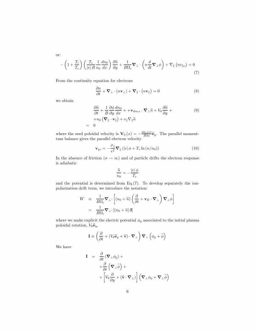
These equations are integrated numerically with a boundary value integrator, afinite difference method. The results are shown in Figures (4), (5) and (6). In thefollowing figures are explained also the functions W1n which will be introducedin Eq.(24).
The first term gives a solution of the following form
φ(2)1n = ϕ
(2)1n exp (ikny − iωnt) + c.c.
where the function ϕ(2)1n satisfies the equation
d2ϕ(2)1n
dx2−(k2
n − β − U ′′
U − cn
)ϕ
(2)1n =
=i
kn (U − cn)
(d2ϕn
dx2− k2
nϕn
)∂An
∂T1
+
[U
(d2ϕn
dx2− k2
nϕn
)+ (β − U ′′)ϕn
−2k2n (U − cn)
] ∂An
∂Y1
This equation serves to generate a condition on the two amplitudes A1,2.When the left hand side of the equation is multiplied by the function ϕn
and integrated between the limits on the x domain, it gives zero, due to theboundary conditions. The same must then be true for the right hand side. This
19
0 0.5 1−100
−50
0
50
100
Source for y21
0 0.5 1−30
−20
−10
0
10
20
30
Source for y22
0 0.5 1−150
−100
−50
0
50
100
Source for y3
0 0.5 1−100
−50
0
50
100
150
Source for y4
0 0.5 1−2
−1.5
−1
−0.5
0
0.5
1
Source for y11
0 0.5 1−4
−3
−2
−1
0
1
2
Source for y12
Figure 5: Graphs of the source terms in the equations for the functions w’s.
0 0.5 1−0.4
−0.2
0
0.2
0.4
Function y21
0 0.5 1−0.2
−0.15
−0.1
−0.05
0
0.05
0.1
0.15
Function y22
0 0.5 10
1
2
3
4
Function y3
0 0.5 10
1
2
3
4
5
6
7
Function y4
0 0.5 1−0.2
0
0.2
0.4
0.6
0.8
1
1.2
Function y11
0 0.5 1−0.01
0
0.01
0.02
0.03
0.04
0.05
0.06
Function y12
Figure 6: Graphs of the functions w’s.
20

gives a “solubility condition”, on the space time scales slower at order 1:
∂An
∂T1+ cgn
∂An
∂Y1= 0
where
cgn = cn + 2
∫ L
0
k2nϕ
2ndx
∫ L
0
β − U ′′
(U − cn)2ϕ2
ndx
Expressed in units of length L and units of time t0 = 10−4, the group velocities
are : cg1 = 0.30328 and cg2 = 3.9908.Then it is clear that the amplitude An propagates at the speed cgn :
An = An (Y1 − cgnT1, Y2, T2)
Now we introduce a new function
ϕ(2)1n = iW1n
∂An
∂Y1
The equation satisfied by W1n is
d2W1n
dx2−(k2
n − β − U ′′
u− cn
)W1n (24)
=1
kn (U − cn)
[(cn − cgn)
(d2ϕn
dx2− k2
nϕn
)− 2k2
n (U − cn)ϕn
]
with the bounday conditions
W1n (0) = W1n (L) = 0
At this order (2) there are the following solutions
φ(2) = φ(2)11 + φ
(2)12 + φ
(2)21 + φ
(2)22 (25)
+φ(2)3 + φ
(2)4 +
+Φ (x, T1, Y1)
The last function will be determined by the condition of solubility at the nextorder on the space-time scales (O
(ε2)). To obtain the evolution equations for
Φ and An, we use the expressions for φ(1) Eq.(21) and φ(2), Eq.(25) in the righthand side of the equation (20), and all inhomogeneous terms are obtained. Inadditions there are terms which are not dependent on y and t, and these termsshould be zero. This leads to the solubility condition relating the function Φ(correction to the mean flow due to the presence of the wave packets) to the
21

amplitude An.(
∂
∂T1+ U
∂
∂Y1
)∂2Φ
∂x2+ (β − U ′′)
∂Φ
∂Y1(26)
=
2∑
n=1
d2
dx2
[kn
(W1n
dϕn
dx− ϕn
dW1n
dx
)]− 4k2
nϕn
dϕn
dx
+
(ϕn
d
dx− dϕn
dx
)(d2ϕn
dx2− k2
nϕn
)∂
∂Y1|An|2
This relation will be used later.Returning to the equation (20), we examine the content of the inhomoge-
neous part (the right hand side). There are terms which have a space-timedependence
exp [ikny − iωnt] (27)
and in order to have solutions of this type, we need to impose solubility condi-tions, otherwise there will arise secular terms at the order φ(3). To find theserestrictions (solubility conditions) we multiply the equation with the functionconjugated to (27)
exp [−ikny + iωnt]
and integrate time on the interval (0, 2π/ωn) and space: y on the interval(0, 2π/kn) and x on the interval (0, L). On the left hand side we obtain zero,so this is what we must obtain also from the right hand side. The conditionswhich results are:(
∂
∂T2+ cg1
∂
∂Y2
)A1 − iα1
∂2A1
∂Y 21
− i(ρ1 |A1|2 + γ12 |A2|2 + λ1
)A1 = 0
(∂
∂T2+ cg2
∂
∂Y2
)A2 − iα2
∂2A2
∂Y 21
− i(ρ2 |A2|2 + γ21 |A1|2 + λ2
)A2 = 0
The notations which have been introduced are: αn = In0
Πn, ρn = Inn
Πn, γ12 = I12
Π1,
γ21 = I21Π2
, λn = In3
Πnand
Πn = −∫ L
0
ϕn
U − cnfndx , In0 =
∫ L
0
ϕn
U − cnfn0dx
Inn =
∫ L
0
ϕn
U − cnfnndx , I12 =
∫ L
0
ϕ1
U − c1f12dx
I21 =
∫ L
0
ϕ2
U − c2f21dx , In3 =
∫ L
0
ϕn
U − cnfn3dx
22
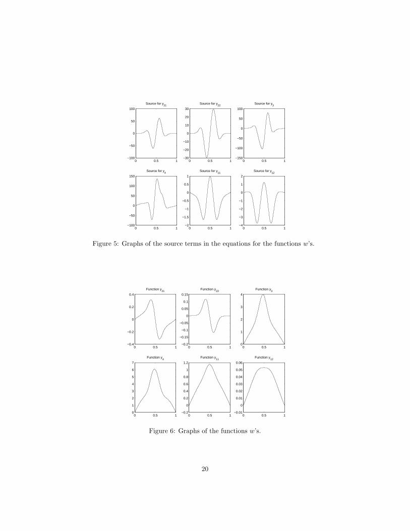
The equations satisfied by all these functions are given given in Ref.([8]).
fn = −(d2ϕn
dx2− k2
nϕn
)
hn = −U(d2ϕn
dx2− k2
nϕn
)− (β − U ′′)ϕn + 2k2
n (U − cn)
fn0 = −2kn (U − cgn)ϕn − kn (U − cn)
− (U − cgn)
(d2W1n
dy2− k2
nW1n
)
+2k2n (U − cn)W1n − (β − U ′′)W1n
fnn = −(
2knW2nd
dx+ kn
dW2n
dx
)(d2ϕn
dx2− k2
nϕn
)
+
(knϕn
d
dx+ 2kn
dϕn
dx
)(d2W2n
dx2− 4k2
nW2n
)
f12 = −(k12W3
d
dx+ k2
dW3
dx
)(d2ϕ2
dx2− k2
2ϕ2
)
+
(k2ϕ2
d
dx+ k12
dϕ2
dx
)(d2W3
dx2− k2
12W3
)
+
(k2ϕ2
d
dx− α12
dϕ2
dx
)(d2W4
dx2− α2
12W4
)
−(α12W4
d
dx− k2
dW4
dx
)(d2ϕ2
dx2− k2
2ϕ2
)
f21 = −(k12W3
d
dx+ k1
dW3
dx
)(d2ϕ1
dx2− k2
1ϕ1
)
−(k1ϕ1
d
dx+ α12
dϕ1
dx
)(d2W4
dx2− α2
12W4
)
+
(k1ϕ1
d
dx+ k12
dϕ2
dx
)(d2W3
dx2− k2
12W3
)
+
(α12W4
d
dx+ k1
dW4
dx
)(d2ϕ1
dx2− k2
1ϕ1
)
fn3 = −kn
(ϕn
∂3Φ
∂x3−(d2ϕn
dx2− k2
nϕn
)∂Φ
∂x
)
23

0 0.5 1−20
0
20
40
60
Function f1
0 0.5 1−10
0
10
20
30
40
Function f2
0 0.5 10
2
4
6
8
10
12
Function h1
0 0.5 10
50
100
150
200
Function h2
0 0.5 1−25
−20
−15
−10
−5
0
5
Function f10
0 0.5 1−20
−15
−10
−5
0
5
Function f20
Figure 7: Graphs of the first group of functions f .
0 0.2 0.4 0.6 0.8 1−1000
−500
0
500
1000
Function f11
0 0.2 0.4 0.6 0.8 1−1000
−500
0
500
1000
Function f22
0 0.2 0.4 0.6 0.8 1−4000
−3000
−2000
−1000
0
1000
2000
3000
Function f12
0 0.2 0.4 0.6 0.8 1−1.5
−1
−0.5
0
0.5
1
1.5x 10
4 Function f21
Figure 8: Graphs of the second group of functions f .
24

We use a boundary value integrator for the inhomogeneous equations and (theNAG routine D02JAF). The results are given in the Figures (7) and (8).
After numerical integrations the follwing values are obtained for the con-stants: α1 = 0.39976, α2 = 0.45246, ρ1 = −0.10182, ρ2 = 1.8115, γ12 =0.091474, γ21 = −5.3768.
The following transformation (Jeffrey and Kawahara) is performed in Ref.([8]) :
T = T2
X =1
ε(Y2 − cg1T2) = Y1 − cg1T1
Then the equation of connection between Φ and An becomes
∂
∂Y
[(U − cg1)
∂2Φ
∂x2+ (β − U ′′)Φ
](28)
=2∑
n=1
[kn
d2
dx2
(W1n
dϕn
dx− ϕn
dW1n
dx
)− 4knϕn
dϕn
dx
−(ϕn
d
dx− dϕn
dx
)(d2ϕn
dx2− k2
nϕn
)]∂
∂Y|An|2
The solution of the equation (28) is considered to be of the form
Φ =2∑
n=1
Hn (x) |An|2 (29)
and the equation for Hn (x) results:
(U − cg1)∂2Hn
∂x2+ (β − U ′′)Hn
= knd2
dx2
(W1n
dϕn
dx− ϕn
dW1n
dx
)− 4knϕn
dϕn
dx
−(ϕn
d
dx− dϕn
dx
)(d2ϕn
dx2− k2
nϕn
)
The change of variables is performed in the equations for the amplitudes An
and, again, the Eq.(29) is used:
i∂A1
∂T+ α1
∂2A1
∂Y 2+(σ1 |A1|2 + ν12 |A2|2
)A1 = 0
i
(∂
∂T− δ
∂
∂Y
)A2 + α2
∂2A2
∂Y 2+(σ2 |A2|2 + ν21 |A1|2
)A2 = 0
where
δ =1
ε(cg1 − cg2)
25

0 0.5 1−20
−10
0
10
20
30
40
50
Potential for H1
0 0.5 1−150
−100
−50
0
50
100
150
Source for H1
0 0.5 1−1
−0.5
0
0.5
1
The function H1
0 0.5 1−1000
0
1000
2000
3000
4000
Potential for H2
0 0.5 1−500
0
500
Source for H2
0 0.5 1−0.4
−0.2
0
0.2
0.4
The function H2
Figure 9: Graphs of the functions H .
σn = ρn − 1
Πn
∫ L
0
knϕn
U − cn
[ϕn
d3Hn
dx3−(d2ϕn
dx2− k2
nϕn
)dHn
dx
]dx
ν12 = γ12 −1
Π1
∫ L
0
k1ϕ1
U − c1
[ϕ1
d3H2
dx3−(d2ϕ1
dx2− k2
1ϕ1
)dH2
dx
]dx
ν21 = γ21 −1
Π2
∫ L
0
k2ϕ2
U − c2
[ϕ2
d3H1
dx3−(d2ϕ2
dx2− k2
2ϕ2
)dH1
dx
]dx
The following transformation is convenient:
A2 = B exp
[iδ
2α2
(Y +
δ
2T
)]
This leads to the following equations:
i∂A1
∂T+ α1
∂2A1
∂Y 2+(σ1 |A1|2 + ν12 |B|2
)A1 = 0 (30)
i∂B
∂T+ α2
∂2B
∂Y 2+(σ2 |B|2 + ν21 |A1|2
)B = 0 (31)
The constants are: σ1 = −1.6324, σ2 = 1.9331, ν12 = −0.53387, ν21 =−2.9014. The constants α1,2 are called the “dispersion”, σ1,2 are called thenonlinearity (“Landau”) constants ; ν12,21 represent the coupling of the twoamplitudes.
26

Numerical experience shows that the dispersion constants are sensitive tothe precision of the integration scheme. We use for D02KEF the value fortolerence 10−8.
The system of coupled Cubic Nonlinear Schrodinger Equations has been inte-grated numerically in relation with many applications [10], [11]. One importantconclusion is that, in the case of a single equation, the sign of the product ofthe dispersion and of the nonlinearity parameters establishes the possibility ofa soliton formation.
3.2 Numerical search for classes of admissible envelopesolutions
In principle an interactive search for eigenvalues (either with SLEIGN or D02KEF)is able to obtain the eigenvalues k1, k2 eventually after series of less-inspiredinitializations. However in many situations resonances occur and the sourcesand/or the potentials in the differential equations for the functions Wn, fn be-come discontinuous. Since these eigenvalues cannot be used we have to devisean automatic search over the space of parameters with checks of continuity ofthe functions and automatic discarding of wrong results. This is accomplishedby the routine P01ABF of NAG.
The search reveals that the short and respectively long radial wavelengthpart of the ion wave spectrum have different behavior under the modulationinstability. The most affected is the long wavelength part (small kx) with ωof the order of the ion-diamagnetic frequency. This corresponds to the domi-nant part of the ion spectrum, because, as can be seen in numerous numericalsimulations, the dominant structures are elongated in the radial direction, withvarious degrees of tilting compared to the radius. It is also important to notethat finding the eigenvalues in the scan of the parameter space weas possible inthe condition that the eigenfunctions ϕ1,2 (x) have low number of oscillations inthe radial direction (one or two). Again this corresponds to the important partof the ITG turbulence spectrum.
The variation of the parameters of the system of NSE with the physicalparameters of the problem can be studied by the automatic search of eigenvalues,as described before. Below are plotted four graphs showing this dependence.
4 Exact solutions of the Nonlinear SchrodingerEquation and the nonlinear stability problem
4.1 Introduction
The Nonlinear Schrodinger Equation can be solved exactly on an infinite spatialdomain using the Inverse Scattering Transform. The first step is to represent thenonlinear equation as a condition of compatibility of two linear equations. Thisis achieved by finding a pair of linear operators (Lax operators) and noticingthat for the first of them the eigenfunction problem is a Schrodinger equation
27

0
100
200
300
400
500
66.2
6.46.6
6.87
7.2
x 105
−0.5
0
0.5
1
1.5
β
Umax
(m/s)
coef
ficie
nt α
1
Figure 10: Parameter dependence of the coefficient α1.
0
100
200
300
400
500
66.2
6.46.6
6.87
7.2
x 105
−1
0
1
2
3
4
β
Umax
(m/s)
coef
ficie
nt α
2
Figure 11: Parameter dependence of the coefficient α2.
28

0
100
200
300
400
500
66.2
6.46.6
6.87
7.2
x 105
0
0.1
0.2
0.3
0.4
0.5
βU
max (m/s)
coef
ficie
nt σ
1
Figure 12: Parameter dependence of the coefficient σ1.
50
100
150
200
250
300
350
400
450
66.2
6.46.6
6.87
7.2
x 105
−2.5
−2
−1.5
−1
−0.5
0
0.5
βU
max (m/s)
coef
ficie
nt σ
2
Figure 13: Parameter dependence of the coefficient σ2.
29

leading to a quantum scattering problem. The unknown function of the NSE isthe potential of the Schrodinger equation. Using the initial condition of the NSEthe scattering data are determined at t = 0. The scattering data have simpletime dependence and so they can be evloved in time to the desired moment. Re-turning from this new set of scattering data (to the potential that has producedit) is achieved by solving an integral equation (Gelfand-Levitan-Marchenko) andprovides the solution of the NSE. In general this solution consists of solitons and“radiation”.
The Inverse Scattering Transform on periodic domain [14], [13], [16] is a morepowerful procedure since it reveals and takes advantage of the deep geometricand topological nature of the problem. The admissible solutions of the Laxeigenvalue problem can now only be periodic functions. Since after one periodthe change of any solution can only be linear (via the monodromy matrix)the periodic or antiperiodic functions must be found as eigenfunctions of thismonodromy operator (matrix), under the constrain that the eigenvalues arecomplex of unit absolute value. This singles out a set of complex values ofthe spectral parameter λ (the formal eigenvalue in the Lax equation), the main
spectrum. From this set, the particular values that make the two eigenfunctionsto coincide are called non-degenerate. Here the squared Wronskian (which isa space and time invariant) has zeros on the complex λ plane. Then the non-degenerate λ’s are singular points for the Wronskian. Removing the square-rootindeterminancy one has to connect pairs of non-degenerate eigenvalues by cutsin the λ plane. The Wronskian becomes a hyperelliptic Riemann surface. Theevolution of the unknown NSE solutions (called hyperelliptic functions µj (x, t))on this surface is as complicated as the original NSE equation. However, viathe Abel map the Riemann surface is mapped onto a torus and on this torus themotion magically becomes linear. After obtaining the space-time dependenceon the torus we need to come back to the original framework. This is called theJacobi inversion and can be done exactly in terms of Riemann theta functions,giving at the end the exact solution of the NSE.
Not only the geometric approach is more clear but it also allows a treatmentof the stability problem for the solutions of the NSE since it allows to trace thechanges of the main spectrum after a perturbation of the initial condition. Thefollowing subsections provide a more detailed discussion of the IST of a periodicdomain. The next section will discuss the stability. This information is availablefrom the abundant literature on the IST and is only mentioned here in orderto understand the mechanism governing the stability of the envelope of the ionwave turbulence. For this reason we will focus on the determination of the main
spectrum and its role in the construction of the solution. The effective steps tobe undertaken to obtain the solution will only be briefly described. We stronglyrecommend the lecture of Ref.([13]) on which this presentation is based.
4.2 The Lax operators and the main spectrum
The IST method starts by introducing a pair of linear operators, called the Laxpair (see [13]) which allow to express the nonlinear equation as a compatibil-
30

ity condition for a system of two linear equations. For the cubic Schrodingerequation
i∂u
∂t+∂2u
∂x2+ 2 |u|2 u = 0 (32)
the Lax pair of operators is
L ≡(
i∂x u (x, t)−u∗ (x, t) −i∂x
)(33)
A ≡(i |u|2 − 2iλ2 −ux + 2iλu
u∗x + 2iλu∗ −i |u|2 + 2iλ2
)(34)
The action of the operators on a two-component (column) wave function φ =(φ1
φ2
)is given by the equations
Lφ = λφ (35)
∂φ
∂t= Aφ (36)
and the condition of compatibility of these two equations φxt = φtx is preciselythe cubic Nonlinear Schrodinger Equation.
4.3 Solving the eigenvalue equation for the operator L
As in the “infinite-domain” IST, we have to solve the eigenvalue equationEq.(35) using the initial condition for the function u (x, t), u (x, 0). How-ever, for the particular case of periodic solutions of the NSE, we must haveu (x+ d, 0) = u (x, 0) where d is the length of the spatial period (i.e. actually Lin the previous notation; however we use d in this and the next section, keepingL for the Lax operator). Fixing an arbitrary base point x = x0 one considersthe two independent solutions of the equation (35) which take the following“initial” values at x = x0:
φ (x0) =
(10
)and φ (x0) =
(01
)(37)
The matrix Φ (x, x0;λ) of solutions is given by
Φ (x, x0;λ) ≡(φ1 (x, x0;λ) φ1 (x, x0;λ)
φ2 (x, x0;λ) φ2 (x, x0;λ)
)(38)
i.e. this solution satisfies the equation
LΦ = λΦ and Φ (x0, x0;λ) =
(1 00 1
)(39)
31

It can be seen that the Wronskian of(φ, φ
)is the determinant of the matrix
of fundamental solutions
W(φ, φ
)= det (Φ)
It can be shown that ∂W∂x = 0 i.e. the Wronskian is constant, which gives
det (Φ (x)) = det (Φ (x0)) = 1
Using the initial condition for Φ one can solve the equation (39) and obtainΦ (x, x0;λ); in particular we can obtain it at x0 + d, i.e. after a period :
Φ (x0 + d, x0;λ) =
(φ1 (x0 + d, x0;λ) φ1 (x0 + d, x0;λ)
φ2 (x0 + d, x0;λ) φ2 (x0 + d, x0;λ)
)(40)
This is called the monodromy matrix and is noted
M (x0;λ) ≡ Φ (x0 + d, x0;λ) (41)
The monodromy matrix is the matrix of the fundamental solutions calculatedfor one spatial period. In general the monodromy matrix is the element of themonodromy group associated to a loop and to its homotopy class, for a markedpoint on a manifold (here the circle S1 ≡ [0, d). The linear monodromy groupacts by replacing the elements of the vector column by linear combinationsof the initial ones. For changes of the marked point x0 the matrix has twoinvariants : the trace and the determinant:
[TrM ] (x0;λ) = [TrM ] (λ) ≡ ∆(λ)
detM = 1
The function ∆ (λ) is called the discriminant and is independent of x0.
Looking for Bloch (Floquet) solutions The values the discriminant ∆ (λ)takes on the complex λ-plane control the monodromy and by consequence selectthe values of λ for which admissible eigenfunction of the Lax problem exist.In other words ∆ governs the spectral properties of the operator L. To findunder what conditions periodic solutions are possible, we construct the Bloch(or Floquet) solutions of the equation Lφ = λφ. The Bloch function has theproperty
ψ (x+ d;λ) = eip(λ)ψ (x;λ) (42)
where p (λ) is the Floquet exponent. Like any other solution of the Laxeigenproblem ψ can be expressed as a linear combination of the two fundamentalsolutions φ and φ
ψ (x;λ) = Aφ (x;λ) +Bφ (x;λ)
32

For the particular point x0 we have, taking into account the “initial” conditions(37)
ψ (x0;λ) = Aφ (x0;λ) +Bφ (x0;λ) =
(AB
)
After one period d the function ψ is linearly modified by the monodromy matrixand, according to Eq.(42) is multiplied by a complex number of unit absolutevalue. We write m (λ) for this number and look for those λ’s where this iscomplex of modulus one. The regions of the λ plane where m (λ) has modulusdifferent of one correspond to unstable functions ψ. We write
ψ (x0 + d;λ) = m (λ) ψ (x0;λ) (43)
M
(AB
)= m (λ)
(AB
)(44)
The Bloch functions are invariant directions for the monodromy operator Macting in the base formed by the fundamental solutions of the Lax eigenproblem.The monodromy operator preserves these directions and multiplies the Blochvector with m (λ) = exp (ip (λ)).
det (M −m) = m2 − (TrM)m+ detM = m2 − ∆(λ)m+ 1 = 0
This gives
m± (λ) =∆ (λ) ±
(∆2 (λ) − 4
)1/2
2
In general ∆ (λ) is an analytic function on the plane of the complex vari-able λ. The equation Im [∆ (λ)] = 0 is a single relation with two unknowns,(Reλ, Imλ) and calculating one of them leaves the dependence on the other asa free parameter. This gives a curve in the plane and the real-λ axis is such acurve: for Imλ = 0 we have Im∆(λ) = 0.
We look at the variation of ∆ (λ) on the complex plane to find the effect onm± (λ).
• Where the Floquet multiplier is a complex number of magnitude unity,the functions are only effected by a phase factor after one period. TheBloch functions (eigenfunctions of L) are stable under translations withd. The real λ axis is a region of stability. The region where ∆ is real and
∆ (λ) < 4
is the band of stability, the modulus of m being 1.
• When λ is such that the discriminant (∆ (λ) ≡ Tr (M) ) is equal to 4,the eigenvalues of the monodromy matrix, m (λ), are ±1, and the Blochfunctions are periodic or antiperiodic. This is the Main Spectrum in λand is noted λj. The main spectrum consists of a set of discrete valuesλj .
33

• for those λ which gives |m (λ)| 6= 1 the Bloch eigenfunctions are unstable.
Consider the case where ∆ (λ) is complex. For all values of the parameter λon the complex plane, [with the exception of the Main Spectrum where ∆ (λ) =±2 ], the eigenvalues of the monodromy matrix are distinct which means thatthe eigenfunctions Bloch are distinct and Independent (The Wronskian isdifferent of zero).
ψ+ (x+ d) = m+ψ+ (x)
ψ− (x+ d) = m−ψ− (x)
However we can only be intersted in points of the main spectrum, as theycan provide admissible (periodic) eigenfunctions of the Lax operator. (1) Thereare points λj in the main spectrum where the two eigenfunctions Bloch aredistinct and independent: these points are called degenerate (with the meaningthat for two independent eigenfunctions there is only one eigenvalue). (2) Thereare points λj where the two eigenfunctions Bloch are NOT independent: thesepoints are called nondegenerate. For such values of λ the Wronskian is zero.
The important class of initial conditions u (x, t = 0) with the property thatthere is only a finite number of non-degenerate eigenvalues λj is called finite-band potential.
4.4 The “squared” eigenfunctions
Starting from the initial condition u (x, 0) and leting it evolve in time according
to the NSE, u (x, 0)NSE→ u (x, t), the discriminant remains invariant. All the
spectral structure obtained from the discriminant ∆ (λ), i.e. the main spectrum,the stability bands, are invariant. The eigenvalues of the monodromy matrix λj
are invariant.
4.4.1 The two Bloch functions for the operator L
Consider the two Bloch eigenfunctions of the operator L:
ψ+ =
(ψ+
1
ψ+2
)and ψ− =
(ψ−
1
ψ−2
)
and define the following functions
f (x, t;λ) ≡ − i
2
(ψ+
1 ψ−2 + ψ+
2 ψ−1
)(45)
g (x, t;λ) ≡ ψ+1 ψ
−1 (46)
h (x, t;λ) ≡ −ψ+2 ψ
−2 (47)
34

These functions have the property that they are periodic, f (x+ d, t;λ) =f (x, t;λ)for all values of λ. Since f is composed of ψ+ and ψ− and theseare Bloch solutions for the eigenvalue equation Lϕ = λϕ we have
∂f
∂x= u∗g − uh (48)
∂g
∂x= −2iλg − 2uf (49)
∂h
∂x= 2iλh+ 2u∗f (50)
and similarly we write the time derivatives taking account of the compatibilitycondition which involves the operator A.
∂f
∂t= − (u∗x + 2iλu∗) g + i (−ux + 2iλu)h (51)
∂g
∂t= 2i
(|u|2 − 2λ2
)g + 2i (−ux + 2iλu) f (52)
∂h
∂t= −2i
(|u|2 − 2λ2
)h− 2i (−u∗x + 2iλu∗) f (53)
It is shown in Ref.([13]) that the condition on the initial function u (x, 0) forthere to be only a finite number of nondegenerate points in the main spectrumis equivalent to the requirement that f, g and h be finite-order polynomials inthe parameter λ, which we take of degree N + 1: f (x, t;λ) =
∑N+1j=0 fj (x, t) λj ,
g (x, t;λ) =∑N+1
j=0 gj (x, t) λj , h (x, t;λ) =∑N+1
j=0 hj (x, t) λj . From the Eqs.(48- 50) it results however that g and h have degree N in λ.
One can check that the following combination is invariant in time and spaceand we note that it is actually the square of the Wronskian:
∂
∂x
(f2 − gh
)=
∂
∂t
(f2 − gh
)= 0 (54)
f2 − gh = −1
4
[W(ψ+, ψ−
)]2
The Wronskian only depends on the spactral parameter λ. We also know that fora subset of the main spectrum, the nondegenerate eigenvalues, the Wronskian iszero. Then the number of the nondegenerate eigenvalues is 2N + 2 (the degreeof f2 − gh as a polynomial in λ) and we express the function f2 − gh as apolinomial with constant coefficients (not depending on x and t).
−1
4
[W(ψ+, ψ−
)]2= f2 − gh ≡ P (λ) =
2N+2∑
k=1
Pkλk =
2N+2∏
j=0
(λ− λj) (55)
35

4.4.2 Product expansion of g and its zeros µj (x, t). Introduction ofthe hyperelliptic functions µj
The functions g and h are both of order N in λ. For g we will note the N rootsby µj (x, t). The coefficient of λ2N+2 in f2 − gh is f2
N+1. Due to Eq.(54) it is
a constant which can be taken 1. Now since fN+1 = 1 the coefficient of λN ing is iu (x, t). Written as a product
g = iu (x, t)
N∏
j=1
[λ− µj (x, t)
](56)
By similar arguments we find that the coefficient of λN in h is iu∗ (x, t) andthe zeros of h are µ∗
j (x, t). The functions µj (x, t) are called the hyperelliptic
functions. It will be proved below that finding the hyperelliptic functions leadsimmediately to the solution u (x, t).
Now we calculate the expression in Eq.(55) for λ = a zero of the function g,i.e. λ is equal to hyperelliptic function µj (x, t):
f2 (x, t;λ = µm) − gh = f2 (x, t;µm) = P (λ = µm)
or
f (x, t;µm) = σm
√P (µm) (57)
Here the factor σm is a sheet index that indicates which sheet of the Riemannsurface associated with
√P (λ) the complex µm lies on.
Let us calculate from Eq.(49) and Eq.(56) the derivative at x of µm:
∂g (x, t;λ)
∂x= i
∂u (x, t;λ)
∂x
N∏
j=1
(λ− µj (x, t)
)
−iu (x, t;λ)
N∑
j=1
∂µj (x, t)
∂x
N∏
k=1,k 6=j
(λ− µk (x, t))
Replace here a zero of g: λ = µm
∂g (x, t;µm)
∂x= −iu (x, t;µm)
∂µm (x, t)
∂x
N∏
k=1,k 6=m
(µm − µk (x, t))
On the other hand we have, from Eq.(49)
∂g
∂x= −2iµmg (x, t;λ = µm) − 2u (x, t;λ = µm) f (x, t;λ = µm)
= −2uf
then, since we have calculated f (x, t;λ = µm), Eq(57), we obtain
∂µm (x, t)
∂x=
−2iσm
√P (µm)
∏Nk=1,k 6=m (µm − µk (x, t))
(58)
36
for m = 1, 2, ..., N .The coefficients of the term with λN in the equation (49) are matched and
we obtain iux = −2igN−1 − 2ufN .Using Eq.(56) we find
∂x lnu = 2i
N∑
j=1
µj + fN
From the Eq.(55) we obtain the coefficient of the term λN , i.e. fN
fN = −1
2
2N+2∑
k=1
λk
Then from the preceding equation it results
∂x lnu = 2i
N∑
j=1
µj −1
2
2N+2∑
k=1
λk
(59)
The same procedure is applied to the equation for gt, (52) and we obtain
∂µj (x, t)
∂t= −2
∑
m 6=j
µm − 1
2
2N+2∑
k=1
λk
∂µj (x, t)
∂x(60)
∂t lnu = 2i
∑
j>k
λjλk − 3
4
(2N+2∑
k=1
λk
)2 (61)
−4i
(−1
2
2N+2∑
k=1
λk
)
N∑
j=1
µj
+
∑
j>k
µjµk
We can see that the problem has been reformulated: from the equationfor the function u (x, t) the Lax-operators formulation leads to the problem forBloch functions, ψ+ and ψ− and their Wronskian; then, using the “squared”eigenfunctions f , g and h we arrive at a formulation for the hyperelliptic func-tions µj (x, t) . Finding µj (x, t) leads immediately to u (x, t).
These operations have a significative geometric counterpart: every point ofthe complex plane of the spectral parameter λ is mapped, via Eq.(55) on the two-
sheeted Riemann surface√− 1
4W (x, t;λ) =√P (λ) with singularities at the
nondegenerate points of the main spectrum, λj . Removing the indeterminancy(by cutting and glueing the two sheets) we obtain a hyperelliptic Riemannsurface of genus g = N . It results that we have to consider the variablesµj (x, t), j = 1, N , as points on this surface but the motion of µj (x, t) is notsimpler than the equation itself.
37

Now the next steps would be: (1) using the initial condition µj (0, 0) on thefunction µj (x, t) we can solve the two equations (58) and (60) and find µj (x, t);(2) then using the initial condition |u (0, 0)| for the function u (x, t) we can solvethe equations (59) and (61). The procedure will be:
• Take the parameters λj | j = 1, 2, ..., 2N + 2 as known; these parametersare non-degenerate eigenvalues from the main spectrum, they can befound from the equation ∆ (λ) = ±2 and ∆ is determined from u (x, 0),the initial condition.
• Choose initial conditions µj (0, 0) and |u (0, 0)| (see below)
• solve the equations for µj (x, t) ; this means to find the hyperelliptic func-
tions. Then solve the equations for u (x, t).
4.5 Solution: the two-sheeted Riemann surface (hyperel-liptic genus-N Riemann surface)
The variable µj ’s are points lying on the two-sheeted Riemann surface associatedwith
√P (λ) =
(2N+2∏
k=1
(λ− λk)
)1/2
≡ R (λ)
which has branch cuts at each of the nondegenerate points λk. Toeliminate the indeterminacy related to the square-root singularities (locatedat λj ’s) the surfaces must be cut and reglued, obtaining a complex manifoldof complex dimension one, a hyperelliptic Riemann surface. We need someconstructions on this surface.
4.5.1 Holomorphic differential forms and cycles on the Riemann sur-face
On this hyperelliptic Riemann surface (denoted M) it is possible to define Nlinearly independent holomorphic (regular) differentials. The following is thecanonical basis of differentials one-forms defined on the manifold M :
dU1 ≡ dλ
R (λ)
dU2 ≡ λdλ
R (λ), ...
dUj ≡ λj dλ
R (λ), ...
38

dUN ≡ λN−1 dλ
R (λ)
On the surface M there are 2N topologically distinct closed curves (cycles).On a torus (N = 1, called elliptic surface) there are two curves which cannot bedeformed one into another. A more general Riemann surface, with N > 1 canbe shown to be equivalent to a sphere with N handles and is called hyperelliptic
Riemann surface. The number N is called the genus of the surface. We have
N = genus of the surface = number of independent holomorphic differential forms
There are 2N cycles which are split into two classes: aj cycles and bj cycles.Each of these cycles has a specified direction (an arrow) attached to it. Toconstruct the cycles, the rules to be applied are:
1. aj cycles do not cross any other aj cycle; bj cycles do not cross any otherbj cycle;
2. the cycle ak intersects bk only once and intersects no other b cycle;
3. the intersection is such that, at the point of intersection, the vector tangentto the cycle ak, the vector tangent to the cycle bk and the normal to thetangent plane of M represent a system of three vectors compatible withthe orientation of M .
This can be represented as:
a a = 0 , b b = 0 , aj bk = δjk
4.5.2 Periods and matrices of periods
With the set of holomorphic differential forms and the set of cycles we can definethe matrices of periods, A and B
Akj ≡∫
aj
dUk
Bkj =
∫
bj
dUk
and the matrices A and B are invertible. A change of basis of holomorphicdifferential forms is a linear transformation represented by the matrix C:
dψj ≡N∑
k=1
Cjk dUk
39

We can choose the matrix C as
C = A−1
Then the periods in the new basis becomes
∫
an
dψj =
N∑
k=1
Cjk
∫
an
dUk =
N∑
k=1
CjkAkn = δjn
∫
bn
dψj = τ jn
where
τ = A−1B
It can be shown that the matrix τ is symmetric τ jk = τkj and has a positive-definite imaginary part Im τ > 0.
4.5.3 The Abel map
The Abel map is defined from the Riemann surface M to the space CN andassociates to a hyperelliptic Riemann surface (a sphere with N hadles) a N -torus. Using the differentials dψj one constructs a change of variables by thefollowing procedure:
• choose a base point on M and call it p0;
• define the variables Wj (x, t) as integrals on the Riemann λ-surface of thedifferential forms from the arbitrary point p0 to the point which is thehyperelliptic function µk (x, t):
Wj (x, t) =N∑
k=1
∫ µk(x,t)
p0
dψj
=
N∑
k=1
N∑
m=1
Cjm
∫ µk(x,t)
p0
λm−1dλ
R (λ)
These variables have the remarkable property that their x and t depen-dence is trivial
d
dxWj (x, t) =
N∑
k=1
N∑
m=1
Cjm
µm−1k
dµk
dx
σkR (µk)
and using
dµk (x, t)
dx= −2iσk
R (µk)∏n6=k (µk − µn)
40

it results
d
dxWj (x, t) =
N∑
m=1
Cjm
N∑
k=1
−2iµm−1k∏
n6=k (µk − µn)
To calculate the sum
N∑
k=1
µm−1k∏
n6=k (µk − µn)
one can use the contour integral
Im ≡ 1
2πi
∫
C
λm−1dλ∏n6=k (µk − µn)
where the contour C encloses all of the poles µn counterclockwise. By theresidue theorem
N∑
k=1
µm−1k∏
n6=k (µk − µn)= Im
One can evaluate this integral by compactifying the λ plane into a sphereand noticing that the contour encloses the pole at z = ∞. Evaluating theresiduu at z = ∞
N∑
k=1
µm−1k∏
n6=k (µk − µn)= δm,N
and from this we obtain
d
dxWj (x, t) = −2iCj,N ≡ 1
2πkj
A similar calculation gives
d
dtWj (x, t) = −4i
[Cj,N−1 +
(1
2
2N+2∑
k=1
λk
)Cj,N
]
=1
2πΩj
It results from these calculations
Wj (x, t) =1
2π(kjx+ Ωjt+ dj)
where dj is a phase which is determined by the initial condition on µk.
The Abel map has linearized the motion of the points µk (x, t). Now, inorder to determine the function u (x, t) we must invert the Abel map, returningfrom the variables W to µ. This is the Jacobi inversion problem.
41

4.5.4 The Jacobi inversion problem
The return from the variables Wj (x, t) of the N -torus back to the variablesµk (x, t) of the Riemann surface M (notice we will only need particular combi-nations of the functions µ) can be done in an exact way using the Riemann θfunction.
The argument of θ is the N-tuple of complex numbers z ∈ CN .
θ (z|τ) ≡∞∑
m1=−∞
· · ·∞∑
mN =−∞
exp (2πim · z + πim · τ ·m)
with the notationsm·z =∑N
k=1mkzk and m·τ ·m =∑N
k,j=1 τ jk mj mk. Addingto the vector z a vector with a single nonzero element in the position k we obtainfrom the definition:
θ (z + ek|τ ) = θ (z|τ)
which means that the θ -function has N real periods. Adding the full k-thcolumn of the matrix τ , we obtain:
θ (z + τk|τ ) = exp (−2πizk − πiτkk) θ (z|τ) (62)
where τkk is the diagonal element of the τ matrix.There are two quantities which must be determined in order to have the
explicit form of the solution. The space and respectively time equations for
u (x, t) depend on the quantity∑
j>k µjµk = 12
[(∑Nm=1 µm
)2
−∑Nm=1 µ
2m
].
So we must determine the following combinations of the variables µj :
N∑
m=1
µm (x, t) and
N∑
m=1
µ2m (x, t)
In order to calculate these two quantities, we shall start by introducing aseries of functions , ψj (p) defined on the Riemann surface M :
ψj (p) =
∫ p
p0
dψj
where p is a point on M , dψj is the j -th holomorphic differential formdefined on M and p0 is an arbitrary fixed point on M . The functions ψj (p) aremultiple valued since the contour is defined up to addition of any combinationof the cycles on M .
Now consider the function, F (p):
F (p) ≡ θ (ψ (p) −K|τ)
where θ is theN -dimensional Riemann theta function associated with the surfaceM ; ψ (p) is the N -dimensional column of complex functions ψj (p); K is an
42

N -dimensional column of complex numbers independent of the point p. Thefunction F (p) is multivalued on the Riemann surface M for the same reason asψ: moving the point p on the surface such as to turn around one of the b cycleand returning to the initial position, the functions ψj will add elements of the τmatrix. This will make the function F to change as imposed by the propertiesof the θ function, shown in Eq.(62).
In order to render the function F single-valued, we replace its domain M bya new surface, obtained from M by dissecting it in a canonical fashion, alonga basis of cycles. This new surface, M∗ is simply connected and has the bordcomposed of a number of arcs equal to 4N .
This operation is necessary in order to render the function F (p) entire andallow us define the inegral
I0 =1
2πi
∫
∂M∗
d lnF (p) (63)
around the contour of the surfaceM∗. Applying Cauchy theorem, the integral isthe number of zeroes of F (p) on the surface M∗. This number is N (Riemann).
We now impose the condition that the N zeros of F (p) coincide with theN points
(µj (x, t) , σj
). This fixes the values of the N complex numbers
Kj (j = 1, ..., N). By doing so the contour integral (63) calculated with thereziduum theorem will involve the variables µj .
Calculation of the two combination of µ’s We must remember that thecomplex λ plane is covered by the two-sheeted Riemann surface whose compactversion is M . Further this is mapped by Abel map onto the Jacobi N -torus. Toa variable on the Riemann surface M (formally also on M∗), say p, correspondsa certain λ (p). One defines the following integrals, which are proved to be realconstants :
I1 =1
2πi
∫
∂M∗
λ (p) d ln [F (p)] ≡ A1
I2 =1
2πi
∫
∂M∗
λ2 (p) d ln [F (p)] ≡ A2
They can be evaluated by the residuu theorem. By the choice of the constantsK’s, the zeroes of the of the function F (p) are located at µj . Then the residuesare just the integrand (λ) calculated in µ plus the residuu at the infinite, ±∞:
I1 =
N∑
m=1
µm + Re sλ→∞+
[λ (p) d lnF (p)] + Re sλ→∞−
[λ (p) d lnF (p)]
I2 =
N∑
m=1
µ2m + Re s
λ→∞+
[λ2 (p)d lnF (p)
]+ Re s
λ→∞−
[λ2 (p) d lnF (p)
]
43
The reason to write two residues at infinity is that λ = ∞ is not a branchingpoint which means that there are two points on the manifold M correspondingto λ = ∞, one on each sheet of the surface. We note r± the value of ψ (p) whenp is the point on M∗ corresponding to λ→ ∞±.
The result is
A1 =
N∑
j=1
µj +i
2
∂
∂xln
[F (r− −K)
F (r+ −K)
]
or
A1 =N∑
j=1
µj +i
2
∂
∂xln
[F (r− −K)
F (r+ −K)
]
with θ± = F (r± −K). The expression of I2
A2 =N∑
j=1
µ2j −
1
4
∂
∂xln[F(r+ −K
)F(r− −K
)]+i
4
∂
∂tln
[F (r− −K)
F (r+ −K)
]
Return to the equations for the function u With these expressions wecome back to the two equations for the two partial derivatives of u.
∂
∂xlnu =
∂
∂xlnF (r+ −K)
F (r− −K)+ 2iA1 − i
2N+2∑
m=1
λm
∂
∂tlnu =
∂
∂tlnF (r+ −K)
F (r− −K)+ iconst
The solution Let us note
ω0 = Q
k0 = 2A1 −2N+2∑
m=1
λm
which are “external” frequency and wavelength.The solution is
u (x, t) = u (0, 0) exp (ik0 − iω0t)θ(W−|τ)θ (W+|τ )
where
W±j =
1
2π
(kjx+ Ωjt+ δ±j
)
The phases δ±j are the part of r± −Kj which is independent of (x, t).
44
5 Stability of the envelope solutions
In this Section we return to the equations obtained by multiple space and timescales analysis. Then the meaning of the variables φ, y, t is: first order (enve-lope) amplitude of the potential fluctuations in the ion turbulence and respec-tively large space and slow time variables. We focus on a single NSE in order toexamine the properties of the stability of the solutions. The equation has thegeneric form
i∂φ
∂t+ α
∂2φ
∂y2+ 2σ |φ|2 φ = 0 (64)
and represents the equation for the envelope of a fast oscillation arising assolution of the barotropic equation. On infinite spatial domain this equationhas soliton as solutions. On a periodic spatial domain (which is our case) thesolutions can be cnoidal waves and they may be modulationally unstable. Theinstability can be examined in the neighbourhood of a solution by imposinga slight deviation and studying its time behaviour by classical perturbationexpansion. This analysis and comparison with the geometric-algebraic resultshave been carried out in Ref.([13]).
Consider φ (y, t) is a solution and perturb it at the initial moment t = 0 as
φ (y, t) = φ (y, 0) + εh (y)
The question is to find the relative behaviour of the two functions φ (y, t) and
φ (y, t). It they depart exponentially for time close to the initial moment, thenφ (y, t) is an unstable solution. Suppose the initial solution φ (y, t) is the envelopeof an exact plane wave i.e. it is constant in space. As a function of time it musthave the form φ (y, t) = p exp (2iqt) and we find
φ (y, t) = p exp(2iσp2t
)(65)
To this solution we add a perturbation
φ (y, t) = p exp(2iσp2t
)1 + ε [A1 exp (iky − iΩt) +A2 exp (−iky + iΩt)]
where A1 and A2 are real coefficients. Linearising the equation for small ε weobtain:
(2p3σ + pΩ − pαk2
)exp (iky − iΩt) + 2p3σ exp (−iky + iΩt)
A1 +
(2p3σ − pΩ∗ − pαk2
)exp (−iky + iΩt) + 2p3σ exp (iky − iΩt)
A2
= 0
Taking the complex conjugate we obtain another equation for the two real co-efficients A1 and A2. The condition of compatibility of this system of equations
45
(the determinant equals zero) can only be fulfilled if the factor multiplying thefunction of y and t is allways zero. This gives us the dispersion relation
Ω = ±√αk(αk2 − 4p2σ
)1/2(66)
which shows that for
|k| < 2 |p|√σ
α
(i.e. for long wavelengths) the two solutions φ (y, t) and φ (y, t) diverge expo-nentially in time and the function φ (y, t) is modulationally unstable. FromEq.(66) we notice that when σ (the Landau coefficient)< 0 and α (the disper-sion coefficient)> 0 the frequency Ω is real and there is no linear instability.This remark is useful in connection with the numerical calculations describedabove, which connect the physical parameters with the coefficients (α, σ) of theNSE. Sampling the space of the physical parameters we must retain those pointswhere the linear instability is possible. In the above formula σ , α and p are di-mensionless constants and the variables of the equation are normalised : time tot0 and length to L. The value of p is connected with the frequency of oscillationof the uniform poloidal envelope ωphys
unif (s−1) by
p =
√t02σωphys
unif (67)
and the condition of linear instability is for the poloidal wavenumber m
m <√
2a
L
√σ
α
(t0ω
physunif
)1/2
(68)
In the case of the following parameters: α = 0.399, σ = 1.452, d = 2πa/L =
2π (1/0.3) = 20. 944, ωphysunif = 105 (sec−1) we have
m . 8
For the Nonlinear Schrodinger Equation it is possible to follow the perturbedsolution much further in time in an exact manner. In Ref.([13]) it is shown thatfrom a solution it is possible to return toward the initial time and to recoverthe results of the linear analysis. This is possible because the equation can beexactly solved for initial conditions starting arbitrary close to the envelope ofthe plane wave. The case of the plane wave (uniform envelope) is particular dueto the simple form of the main spectrum, as will be discussed below.
5.1 Modulation instability of the envelope of a plane wave
5.1.1 General method
The geometric-algebraic setting of Inverse Scattering Transform is the appro-priate framework for understanding the nature of the stability of the exact
46

solutions of the NSE. This is because the solution is strongly dependent onthe topology of the hyperelliptic Riemann curve which in turn is dependent onthe initial function. A perturbation of the initial condition may change themain spectrum turning degenerate eigenvalues into new nondegenerate pairs ofeigenvalues. This means that the hyperelliptic curve will have a different genusN ′ > N and new cycles and differential forms should be defined. The solutiondepends precisely on this topology.
We order to investigate the stability of an exact N -band solution of the NSEwe have to develop in detail the construction of solution. In the particular casewhere the solution is the plane wave this analysis is simpler since all the spectralproperties can be found analytically. It has been proved [13] that under theperturbation of the initial condition the degeneracies in the main spectrum willbe removed and new degrees of freedom will become active. In the new solutionsome of the new degrees of freedom have little effect and can be neglected.
5.1.2 Calculation of the main spectrum associated to the uniformamplitude solution
The unperturbed solution is the envelope of the plane wave, Eq.(65). To de-teremine the main spectrum, the solution is considered initial condition (att = 0) and introduced in the Lax operator. The eigenvalue problem of the Laxoperator has the form
(i√
σα
∂∂y 1
−1 −i√
σα
∂∂y
)Φ = λΦ
where
Φ ≡(φ1
φ2
)
The equation is:
∂2φ1
∂y2+α
σ
(1 + λ2
)φ1 = 0
The general solution is written
φ1 = A cos (κy) +B sin (κy)
κ =
√α
σ
√1 + λ2
The second component will be also a combination of harmonic functions:
φ2 = C cos (κy) +D sin (κy)
47

The equation can have two independent one-column solutions. The one corre-sponding to the boundary conditions
Φ1 (y = 0;λ) ≡(φ1
φ2
)
y=0
=
(10
)
is determined by A = 1, B =√α/σ λ/ (iκ) , C = 0 and D =
√α/σ i/κ. The
solution is
Φ1 (y;λ) =
(cosκy − λi
√ασ
sin κyκ
i√
ασ
sin κyκ
)(69)
The second fundamental solution corresponds to the initial condition;
Φ2 (y = 0;λ) =
(01
)
and it results:
Φ2 (y;λ) =
(i√
ασ
sin κyκ
cosκy + λi√
ασ
sin κyκ
)(70)
The fundamental solution matrix Φ is a 2 × 2 matrix having as column thetwo above solutions. From the fundamental solution matrix we calculate themonodromy matrix
M (λ) ≡ Φ (y = d;λ)
The discriminant is the trace of the monodromy matrix.
∆ (λ) = 2 cos
(d
√α
σ
√1 + λ2
)(71)
We can proceed to the calculation of the spectrum.
5.2 The spectrum of the plane wave solution
5.2.1 The spectrum of the unperturbed initial condition (case ofplane wave)
We take a set of constants as derived from the numerical calculations thatconnects the physical conditions to the coefficients of the NSE, d = 2π
(aL
), α =
0.399, σ = 1.452. With these constants we calculate the spectrum on thecomplex λ-plane. Although we can have analytical solutions the graphs belowshow the difficulty of resolving the details of the variation of the functions. Tobe noted that the function is intersected with a plane arbitrarly placed at themagnitude TrM = 5, for easier 3d-representation.
This graph shows the presence of roots on the imaginary axis of λ of theequation |TrM (λ) − 2| = 0 with very narrow variation of the function. Actually
48

Figure 14: Absolute value of Tr(M)−2. The zeroes on the Imλ axis are difficultto resolve.
it is easily to see that for the parameters adopted here, there are three roots ofthis equation, while in the graph we can hardly see two of them. A graphicalbetter way of finding these roots is to look for the intersections of the contoursof the two equations:
Re (TrM) − 2 = 0
Im (TrM) = 0
where, again, the other two roots cannot be easily resolved. However theanalytical expression allows to find the positions of the roots both on the Reλaxis and on the Imλ axis:
By contrast, the variation along the real λ axis easily evidences the zeroesof the corresponding to the main spectrum.
The stability or instability of the Bloch fuctions (i.e. the values of thequantity m (λ) which is the eigenvalue of the monodromy matrix) is governedby the discriminant ∆(λ). We have −2 6 ∆(λ) 6 2 for all real λ and forλ = iα with −1 6 α 6 1. The main spectrum corresponds to the values of λ forwhich ∆ (λ) = ±2. For real λ, λ ≡ λ0
n,real this means
λ0n,real = ±
(
nπ
d√α/σ
)2
− 1
1/2
49

−1.5 −1 −0.5 0 0.5 1 1.5
−1
−0.8
−0.6
−0.4
−0.2
0
0.2
0.4
0.6
0.8
1
Re λ
Im λ
Figure 15: Contours of the solutions of: TrM − 2 = 0 and ImTrM = 0.
−1 −0.8 −0.6 −0.4 −0.2 0 0.2 0.4 0.6 0.8 1−3
−2
−1
0
1
2
3
λ (imag)
Re[
TrM
(λ )
]
Along the Imλ axis: Im(TrM)=0, Re(TrM) can have three zeros
Figure 16:
50

−1.5 −1 −0.5 0 0.5 1 1.5−3
−2
−1
0
1
2
3
λ (real)
TrM
(λ )
Figure 17:
for n ≥ 3. For pure imaginary λ, λ ≡ iλ0n,imag
λ0n,imag = ±
1 −
(nπ
d√α/σ
)2
1/2
for n = 0, 1, 2 (with the values of the parameters α, σ and d). These values are:iλ0
0,imag = ±i, iλ01,imag = ±i0.9422 and iλ0
2,imag = ±i0.7424. Since d is finiteonly a finite number of degenerate pairs will appear on the imaginary axis. Atn = 0 there are two eigenvalues λ0 = ±i . These eigenvalues are nondegenerate
in the sense that there is only one Bloch function for each of these values of λ.This can be shown directly, constructing the Bloch functions form the matrixof fundamental solutions (69) and (70) with κ → 0 (because ∆ (λ) = 2 impliesκ = 0) and showing that only one Bloch function can be obtained.
5.2.2 The spectrum of the perturbed initial condition (case of planewave)
Starting from an initial condition slightly different of the plane wave’s envelope
u (y, 0) → u (y, 0) + εh (y) (72)
we shall have to repeat all steps in the determination of the spectrum. This mustbe done in a comparative manner, identifying the degenerate eigenvalues λj ofthe main spectrum which becomes nondegenerate after perturbation. The timebehaviour of the exact solution developing from the perturbed initial conditionis dominated by the imaginary part of the variables W which are obtained onthe basis of the new (perturbed) quantities µj and this can be calculated.
51

Figure 18: The graph of Tr(M) − 2 showing the zeroes on the Reλ axis.
52
Using the new initial condition Eq.(72) we shall calculate the new mainspectrum, i.e. the new values of the parameter λ for which the discriminantis ±2. All the spectrum of the simple initial condition u (y, 0) is perturbed byorder-ε quantities. The main effect of this perturbation is that the degeneraciesare broken. In order to construct the exact solution corresponding to the newposition of the nondegenerate λ values, we need to specify the cycles on the two-sheeted Riemann surface. The steps are as usual and consists of first choosingthe cycles on the Riemann surface and the base of the holomorphic differentials;then, compute the matrices of periods (the matrix of a periods, and the matrixof the b periods); compute the τ matrix; construct the Abel map, which mapsthe points of the compact two-sheeted Riemann surface onto the Jacobi torus;find the wavenumbers and the frequencies in the Jacobi manifold; make theJacobi inversion, using the theta functions;
Finding the base of the holomorphic differentials One of the eigen-value pair of the unperturbed system is (−i, i). Consider now that underthe perturbation a degenerate eigenvalue λ0
j splits into the conjugated pair(λ0
k − εk, λ0k + εk
). In Ref.([13]) it was constructed a new basis as a linear
combination of the canonical basis:
dUj =1
2πi
√1 +
(λ0
j
)2∏
m 6=j
(λ− λ0
m
)dλ
R (λ), for j = 1, 2, ..., N
where
R (λ) =√
1 + λ2N∏
k=1
[(λ− λ0
k − εk
) (λ− λ0
k + εk
)]1/2
To understand the choice of basis it is useful to look at the limit ε→ 0 wherethe basis of holomorphic differential becomes
limε→0
dUj =1
2πi
√1 +
(λ0
j
)2 1√1 + λ2
dλ(λ− λ0
j
)
This expression shows that, at the limit ε→ 0, each differential “sees” only onepole, at λj (which is a double point at this limit), and the square-root branch
points ±i.The loop (cycle) aj encircles the pole λ0
j and the period is
limε→0
Akj = limε→0
∫
aj
dUk =
∫
aj
limε→0
dUk = δkj
This is because the cycle aj surrounds the pole λ0j or it does not surrounds any
other pole.We find that, under the limit operation ε → 0, the matrix A goes over to
the identity matrix to the first order in ε, O (ε) and that the matrix B becomes
limε→0
Bjk = τ jk +O (ε)
53

To see what happens with the B matrix in this limit, we must examine theoff-diagonal terms and the diagonal terms.
The off-diagonal terms are well-behaved and can be integrated analytically:
limε→0
Bjk =
∫
bj
limε→0
dUk for j 6= k
and
τkj =1
2πi
√1 +
(λ0
j
)2 ∫
bj
1√1 + λ2
dλ(λ− λ0
k
) + O (ε)
The contour bj passes through the middle of the segment connecting the twonew λj and goes around the pole at λ = −i, for example. If this contour doesnot surround the pole at λ0
k then the integral is elementary. If the contourintersecting the cut from −i to infinity encircles the pole at λ0
k then it maybe chnaged such that to intersect the other cut, connecting the branch point+i to infinity, and so it does not encircle any pole. In conclusion since theoff-diagonal elements of the matrix τ depend (to 0 (ε)) only of the positions ofthe original double points, which are determined only by the parameter d, itresults that: the off-diagonal terms of the τ matrix does not carry anyinformation on the perturbed initial condition. Only the diagonal termsof the τ matrix are affected by the initial condition.
The diagonal terms of the τ - matrix are singular at the limit ε → 0.Consider
τkk =1
2πi
√1 +
(λ0
j
)2 ∫
bk
1√1 + λ2
dλ√(λ− λ0
k
)2 − ε2k
+O (ε)
Suppose that
λ0k is on the imaginary axis
Then we have
τkk =1
2πi
√1 +
(λ0
j
)2(
2
∫ λ0k
−i
+1
2
∫
ak
)1√
1 + λ2
dλ√(λ− λ0
k
)2 − ε2k
+O (ε)
τkk =1
2+
1
πi
√1 +
(λ0
j
)2 ∫ λ0k
−i
1√1 + λ2
dλ√(λ− λ0
k
)2 − ε2k
+O (ε)
The integral can be made with elliptic functions but an approximation is (nearεk = 0)
τkk =1
2− i
πln |εk| +O (1) +O (εk)
54

Consider now
λ0k is on real axis
then the integral defining the diagonal elements of the matrix τ (the integralalong the bk cycles) is
∫ λ0k
−i
=
∫ 0
−i
+
∫ λ0k
0
where the second integral is along the real axis.The first integral is done with the residuu theorem after taking safely the
limit εk = 0 and gives a finite imaginary contribution which is well-behaved forthis limit. The second can be done and the result is
τkk = − i
πln |εk| + iO (1) +O (εk)
We then conclude that for εk → 0 the b - period matrix τ becomes logarith-mically singular on the main diagonal.
The main conclusion is: (1) The real-λ axis degenaracies have Ωj real sothey are linearly stable. The imaginary axis degeneracies have Ωj imaginary sothey are linearly unstable.
This conclusion can have important practical effects: in our case the de-generate eigenvalues on the imaginary λ-axis split and induce instability of theplane wave solution, i.e. of the envelope. At the same time the solutio evolvestoward one of the stable (soliton-like) solutions. Still much work is required toexamine the stability of that solution to additional perturbation. For example,the main spectrum of the solution of the type sech(y) can be obtained fromthe discriminant whose form is very complicated, with many purely imaginary(dangerous) eigenvalues.
6 The growth of the perturbed solution as asource of poloidal asymmetry and spontaneous
plasma spin-up
6.1 The minimal condition for instability of the poloidalrotation
We have found that the space-uniform solution (poloidal symmetry) is unstableand the turbulence will self-modulate according to one of the possible soliton-like solution. In a time picture, we can say that the poloidal symmetry willbe left and the turbulence amplitude will develop a poloidal asymmetry whichgrows exponentially in time. The onset of the poloidal asymmetry will induce anasymmetric rate of transport on the poloidal direction [12]. When the particlediffusion is poloidally asymmetric and the local particle confinement time is
55

Figure 19: The discriminant TrM (λ) of the sech (y) solution, to compare withthe plane wave solution’s discriminant.
shorter than the damping time of the poloidal rotation, the poloidal rotationis unstable. The plasma can spontaneously spin-up. The growth rate of theasymmetry (which is given by the rate of departure from the uniform solutiontoward a soliton-like solution) determines the growth rate of the torque appliedto plasma in the poloidal direction but the relation is not direct, dependingessentially of the momentum balance in the poloidal direction. Any torqueacting to generate a poloidal rotation must overcome the neoclassical magneticpumping, which is an efficient damping mechanism. A balance of these forcesdepends on the comparison between the rates of (1) asymmetry growth, theradial variation of the asymmetry-induced terms, on one hand, and (2) rate ofdamping through magnetic pumping, on the other hand.
For the simplest case of the space-uniform envelope solution, we have theinstability has the linear growth rate
iγenv = i ImΩ = i∣∣∣√αk(αk2 − 4p2σ
)1/2∣∣∣
where k < 2p√σ/α is here the wavenumber of the perturbation of the envelope.
In the case that has served as example in the preceeding Section, we have
p =√t0ω
physunif/ (2σ) ≈ 1.86 and k < 7.08. Taking for example k = 3 we obtain
γenv = 7.67 or γenvphys = 7.67 × 10⁴ (s−1).
6.2 The soliton developing from the initial perturbation
Since we know that the uniform state can be unstable we have to investigatethe problem of the evolution of the system after a perturbation is applied andlook for stable solutions. The solitons of this system can be realisable in real
56

conditions since they are intrinsically more stable. We will look for soliton-likesolution for the uncoupled equations, taking a single NSE like (64). The timedependence can be
φ = exp(iµ2αt
)w (x)
giving the reduced equation
∂2w
∂x2− µ2w +
σ
αw3 = 0
where µ is a real constant. This equation has the following solution
w =
√2α
σµ sech (µx)
The constant µ can be related to the modulation wavenumber whose upperbound is (68). Taking µ ≃ 3 and α = 0.399 we obtain the frequency of steadilyoscillating soliton ωenv
osc ≡ µ2α ≃ 1.2, which is slower than the growth rateof the deformation, γlin = 7.67 obtained above (all in absolute units). Sincethe rate of change of the poloidal velocity (which will be calculated below) hascomparable magnitude with ωenv
osc we conclude that the rotation has the timeto develop before the oscillation reverses the sense of the applied torque. Themaximum amplitude of the deformation is
√2α/σµ = 2.224. Large smooth
deformations (small µ) with less localised profile will have even slower steadyoscillatory motion and however significant amplitude, and we can expect theyare favored in real situations.
6.3 The poloidal asymmetry of the diffusion fluxes
Our approach, which is adapted to the investigation of the stability of the tur-bulence envelope, can only provide a model of the turbulent field, according toEq.(21). This is composed of the primary modes propagating in the poloidal di-rection with amplitude modulated by the slowly varying envelopes A1,2 obeyingthe system of coupled Nonlinear Schrodinger Equations (30) and (31). In theradial direction the field has a variation given by the functions ϕ1,2 (x) obtainedby solving the equations (22). We will need to reconstitute the turbulent fieldin order to calculate the modified diffusion coefficient. We choose the followingset of parameters:
a = 1 (m)
BT = 3.5 (T )
Te = 1 (KeV ) , Ti = 1 (KeV )
n = 1020(m−3
)
Ln = 0.1 (m)
57
U0 = 6 × 10⁵ (m/s)
The extension on the radial direction of the mode is taken L = 0.1 (m) andthis is also the normalising length. Other quantities are: normalising timet0 = 0.16 × 10⁻⁶ (s) and Ωi = 0.335 × 10⁹
(s−1), the ion-cyclotron fre-
quency. From this it results the two parameters of the barotropic form ofthe ion mode, β = 111.75 and ε = 0.476 × 10⁻². We take the followingfrequencies for the primary poloidal modes: ω1 = 0.1451 × 10⁶
(s−1)
and
ω2 = 0.1931 × 10⁶(s−1). From the solution of the equations (22) the two
eigenvalues result: k1 = 43.51(m−1
)and k2 = 56.81
(m−1
). Solving the series
of differential equations described in detail in Section 3 we obtain the followingconstants in the coupled Nonlinear Schrodinger Equations: α1 = 0.1756×10⁻² ,α2 = 0.2278×10⁻² and respectively σ1 = 0.18272 , σ2 = 0.5110. The frequencyof the uniform oscillations, Eq.(67) is taken p = 0.0675 giving the maximumpoloidal number for the large scale instability, Eq.(68), m = [5.89] = 5. Thegrowth rate of the modulational instability is γ = 4175
(s−1). The expression
of the field becomes
φ (r, θ) = φ0 [(1 +A1 (θ) sech(y)) cos (k1y − ω1t+ δ1)ϕ1 (r)
+(1 +A2 (θ) sech(y)) cos (k2y − ω2t+ δ2)ϕ2 (r)]
where φ0 is explained below. The initial phases δ1,2 are arbitrary and in thenumerical calculations are taken as random quantities with uniform distributionon the interval (0, 1).
We notice that the equations (22) fulfilled by ϕ1,2 are homogeneous and theamplitudes of the two functions are arbitrary. We fix the amplitude φ0 withthe condition that the uniform profile of the averaged square of the potentialof the fluctuating field obtains a typical value of the diffusion coefficient, D0 ∼⟨|φ0|2
⟩, which is taken D0 ∼ 1
(m2/s
). The following two figures represent the
fluctuating potential, resulting from the combination of the factors describedabove.
A simple way to take into account the effect of the turbulence amplitudemodulation on the diffusion coefficient is to consider that locally the diffusion
coefficient is proportional with the quantity⟨|φ|2
⟩, where the averages should
be taken over a statistical ensemble of realizations of the fluctuating field. Thisrequires a carefull examination when applied to numerical calculations. We haveto remember that the diffusion is a statistical process where a test particle inter-acting with fluctuating background field performs random displacements whosemean square grows linearly in time. The random displacements have to belongto a Gaussian statistical ensemble and this requires that all kind of elemen-tary experiences (i.e. displacements) to be represented with the correspondingprobability. This is practically irrealisable in numerical calculations since thestatistical ensemble of the stochastic field configurations is necessarly finite, i.e.incomplete as a Gaussian ensemble. Any average will be made on subensem-bles, more or less incomplete. The collection of field configurations are obtained
58
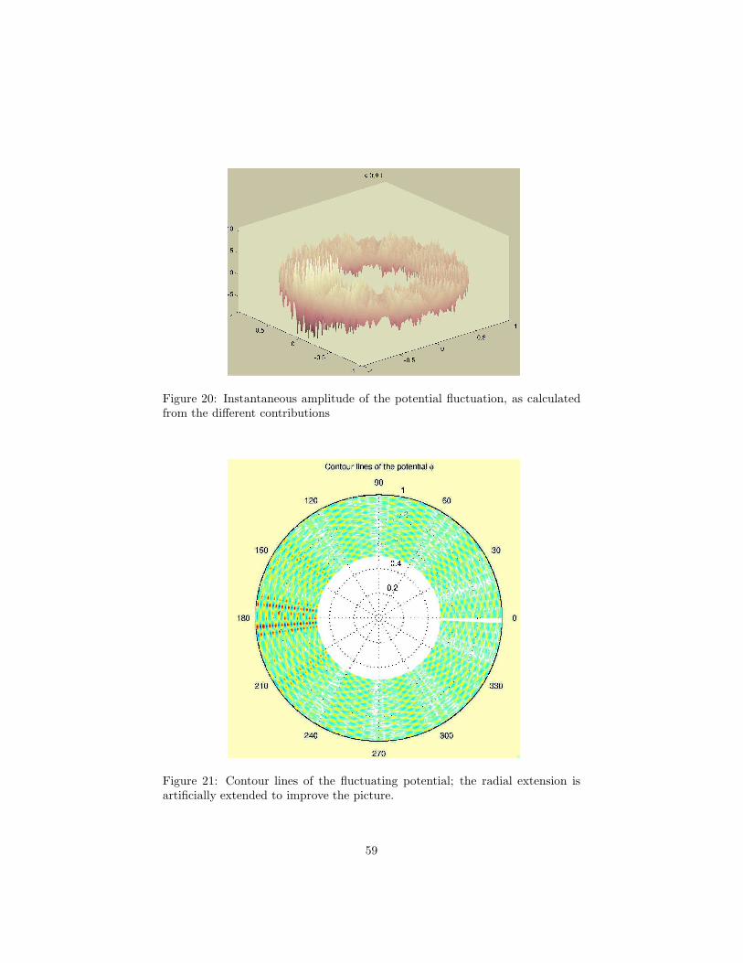
Figure 20: Instantaneous amplitude of the potential fluctuation, as calculatedfrom the different contributions
Figure 21: Contour lines of the fluctuating potential; the radial extension isartificially extended to improve the picture.
59

Figure 22: The radial and poloidal dependence of the average diffusion coeffi-cient.
from time and from space realizations of the field. The test particle should havethe possibility to manifest the linear mean square displacement specific to theGaussian ensembles and this rises the question on what is the minimal spatialextension on which the average should be done. We need in any case a spaceregion larger than the correlation length of the fluctuating field which can betaken as the inverse of the characteristic wavenumber in the field (minimum ofk1, k2).
The profile of the quantity D0
⟨|φ|2
⟩is represented in the figure below. The
exemple chosed for these graphical representation is characterized by the im-posed constrain to obtain a rapid variation of the functions ϕ1 and ϕ2 on theradial r-interval, with the intention to simulate short wavelength ion turbulence,frequently observed in the numerical simulations of the Ion Temperature Gra-dient driven turbulence. This is achieved by asking the numerical procedureswhich solves the Schrodinger-type equations (22) to look for high order κ ofthe eigenvalues. The pictures represented in this section correspond to κ = 19for both eigenfunctions. This generates a potential dominated by small spatialscales and consequently, the fast variation of the local value of the diffusioncoefficient. We take, in the case κ = 19 a space region containing at leastthree complete oscillations of the typical wavelength. This should allow at leastseveral random steps in the typical displacement of the particle. When we dothis (taking arbitrarly a factor of few units larger than the correlation length)we note that the diffusion coefficient exhibits space variations. These are nat-ural and are inherited from the space dependence of the radial eigenfunctionsϕ1,2 (r). Since in real situations the radial eigenfunctions are superposed withrandom initial phases we need to enlarge the region of averaging over most of theradial interval considered, up to a level of saturation of these spatial variationwhich can be considered convenient for the estimation of the poloidal torque.
60

0 0.01 0.02 0.03 0.04 0.05 0.06 0.07 0.08 0.09 0.11.9
1.91
1.92
1.93
1.94
1.95
1.96
1.97
radial coordinate on the interval L
diffu
sion
coe
ffici
ent
Figure 23: Radial variation of the diffusion coefficient after poloidal averaging.
6.4 The poloidal torque applied on plasma
We use the equations describing the plasma poloidal and toroidal rotation de-rived in [17], [18]:
∂n
∂t+
1
r
∂
∂r(rnvr) = 0
∂
∂t(nVϕ) +
1
r
∂
∂r[rn (Vϕvr − qVθ vr)] = 0
∂
∂t
[Vϕ + Θ
(1 + 2q2
)Vθ
]+ vr
∂Vϕ
∂r− vr
∂
∂r(qVϕ) + magnetic pumping = 0
The definition of the variables is n = 〈n (r)〉, nVϕ (r) ≡⟨nvϕ
RR0
⟩and Vθ (r) =
⟨vθ
RR0
⟩, where vϕ and vθ are local toroidal and poloidal plasma velocities in
the magnetic surface. The magnetic field is
B = (0,Θ (r) , 1)B0 (r)
R/R0
with R = R0 + r cos θ and q = rR0
1Θ . The surface average is made according to
the formula
〈f〉 =
∮dθ
2π
R
R0f
61

In the collisional regime the magnetic pumping term determined by parallelviscosity is less effective and the spin up can be expected. The decay rate ofthe poloidal rotation by this mechanism is [19]:
γMP ≃ 3
4
(1 +
1
2q2
)−1(l
qR
)2
νii (73)
where l is the mean-free path. The velocities vr and vr arise from the diffusiveflux in the radial direction, to which is associated the local radial velocity Vr.We define the two velocities
vr = 〈Vr〉
vr = 〈2 cos θ Vr〉 (74)
If there is no poloidal variation of the local radial velocity Vr the average in (74)is that of the trigonometric function cos θ and the result is zero. The averagewill not be zero if there is a poloidal variation of the diffusion-generated particleradial velocity, Vr (θ). We can introduce the modified diffusion coefficient Drelated to the nonsymmetry,
nvr = Γr = −D ∂n∂r
(75)
with
D =⟨D0
⟨|φ|2
⟩st
2 cos θ⟩
pol(76)
where the first averaging is statistical and the second is on the poloidal surface.The equation for the plasma poloidal velocity is
Θ(1 + 2q2
)(∂Vθ
∂t+ γMPVθ
)+ qVθ
1
nr
∂
∂r(nrvr) = 0 (77)
The average velocity Eq.(75) still dependes on the radial coordinate via D0, thedensity n (r) and its derivatives and, more important, via the space dependenceof the potential ϕ (x) left after the statistical averaging needed for the calculationof the diffusion coefficient (76). The following quantity must be numericallycalculated
γ ≡ −qΘ (1 + 2q2)
1
nr
∂
∂r(nrvr) =
q
Θ (1 + 2q2)
1
nr
∂
∂r
(r⟨D0
⟨|φ|2
⟩st
2 cos θ⟩
pol
∂n
∂r
)
and this directly provides the rate of change of the poloidal velocity due to theasymmetry. This must be compared to the magnetic pumping term (73) andwe expect rotation instability when
γ − γMP > 0
62

0 0.01 0.02 0.03 0.04 0.05 0.06 0.07 0.08 0.09 0.10
20
40
60
80
100
120
radial coordinate on the interval L
γ (s
−1 ),
rat
e of
cha
nge
of V
θ d
ue to
asy
mm
etry
Figure 24: Radial variation of the rate of time variation γ applied on plasma inthe poloidal direction, due to the asymmetry.
In this formula the soliton profile of the poloidal asymmetry is considered satu-rated and the motion of the solitons (which would give periodic variation of thetorque) is neglected. As is shown in Ref.[17] the high positive second derivativeof the density profile, combined with a dependence of the diffusion coefficientD0 on the shear of the poloidal velocity are the favorable circumstances forthe asymmetry-induced torque to overcome the magnetic pumping term and aspontaneous spin up to occur. We do not take into account the variation of D0
with the velocity shear, but notice that the space variation of (76) also con-tribute to obtain a positive value for γ sufficient for being comparable to γMP
and even to be larger. The most important contribution comes however fromthe positive-valued second density gradient, which can be seen as an indicationthat the spin-up can be expected in such region on the minor radius.
The values represented in the figure have been calculated using a gaussianprofile for the density. The decay due to magnetic pumping is of the order ofγMP ∼ 12
(s−1). We note that the torque applied to plasma shows a radial
variation essentially inherited from the space variation of the statistically aver-aged potential fluctuations, which in general are not monotone functions of theradius on time scales of several eddy turn-over times. These spatial variationsof the diffusion coefficient generate the profile of the torque which change theshear of the seed velocity and provide a characteristic which is expected forzonal flows. Even outside the domain of the parameters where the spin up isefficient compared to the magnetic pumping, the soliton asymmetry and theStringer torque can contribute to the action of other mechanisms to generatepoloidal rotation.
63

7 Discussion
We have examined the problem of stability of the envelope of the ion wave turbu-lence. Starting from a simple model for the ion dynamics and retaining the fullnonlinear contribution of the ion polarization current we have derived an equa-tion of the same form as the barotropic model of the atmosphere. The multiplespace-time scale analysis shows that the envelope of the turbulence results froma set of coupled cubic nonlinear Schrodinger equations. The simplest solution isthe space-constant envelope corresponding to a symmetric average amplitude ofthe turbulence on the poloidal circumference. In order to examine the stabilityof this solution we first review the method of inverse scattering transform inthe geometric-algebraic framework, able to obtain the exact solution developingfrom a certain class of initial conditions (finite-band potentials). In this frame-work appears clear the origin of the sensitivity to the perturbations, connectedto the topology of a hyperelliptic Riemann surface. The uniform solution isunstable and evolves to one of the soliton-type solution. The nonuniformity ofthe turbulence average profile generates a torque on the plasma, which may besufficient to overcome the poloidal damping.
The simple physical model we have employed may be partly justified by theobservation that the analysis is essentially independent of the other possiblesources of poloidal asymmetry: the neoclassical variation of parameters on themagnetic surface, the toroidal effect on the nonlinearity represented as modecoupling, the effect of the particle drifts on the linear and renormalized propa-gators, etc. The cubic nonlinear Schrodinger equation has many solutions on theperiodic domain and the relevance for the self-modulation of the envelope of theturbulence should be examined. Here we only considered the uniform envelopesince its instability can be sufficient to induce plasma poloidal rotation. Thisrotation has an origin different of the usual sources of rotation: neoclassical,ion-loss, Reynolds stress or momentum injection. Our approach is essentiallymathematical and so it operates at a more formal level. The physical originof the instability seems to be the tendency of the system (averaged amplitudeof the turbulence) to evolve to profiles characterised by the balance of the dis-persion and the nonlinearity. What remains to be examined is the quantitativeconstraint on the minimal initial perturbation needed to produce a particularevolution: for a weak perturbation the solution may be simple “radiation” whilefor initially larger amplitude a soliton emerges ensuring higher robustness anda localised form. It is in this case that the asymmetry can induce plasma ro-tation. This question can be answered by examining the exact solution, withspecific numerical tools for the determination of the main spectrum. It mightbe possible that the Riemann curve is not a hyperelliptic surface but a manifoldclose to a finite-genus curve.
Aknowledgements. The authors gretefully aknowledge the useful discus-sions and encouragements form J. H. Misguich and R. Balescu. The hospitalityof the Departement de Recherche sur la Fusion Controlee (Cadarche, France)is aknowledged. This work has been partly supported by the NATO LinkageGrant PST.CLG.977397.
64
References
[1] T. E. Stringer, Phys. Rev. Lett. 22 770 (1969).
[2] S. Champeaux, P.H. Diamond, “Streamer and zonal flow generationfrom envelope modulations in drift wave turbulence”, Phys.Letters A288(2001)214-219.
[3] K. Itoh, S.-I. Itoh, M. Yagi and A. Fukuyama, “Solitary Radial ElectricField Structure in Tokamak Plasmas”, Report NIFS-525, Dec.1997.
[4] K.H. Spatschek, S.K. Turitsyn and Yu.O. Kivshar, “Average EnvelopeSoliton Dynamics in Systems with Periodically Varying Dispersion”,Phys.Lett.A204, 269-273 (1995).
[5] E. W. Laedke, O. Kluth and K. H. Spatschek, “Families of Discrete SolitaryWaves in Nonlinear Schrodinger Equations”, in E. Alfinito, M. Boiti, L.Martina and F. Pempinelli, eds. (World Scientific, Singapore, 1996) 521-528.
[6] A. V. Tur, A. V. Chechkin and V. V. Yanovsky, Phys. Fluids B 4, 3513(1992).
[7] W. Horton, Phys. Reports 192, 1 (1990).
[8] B. Tan, J. Atmospheric Sciences 53, 1604 (1996).
[9] B. Tan and J. P. Boyd, Chaos, Solitons & Fractals 11, 1113 (2000).
[10] V. I. Pulov, I. M. Uzunov and E. J. Chacarov, Phys. Rev. E 57, 3468(1998).
[11] J. Yang, Physica D 108, 92 (1997).
[12] See file: www.ipp.cas.cz/tokamak/turbmovie.html.
[13] E. R. Tracy and H. H. Chen, Phys. Rev. A 37, 815 (1988).
[14] S. Novikov, S. V. Manakov, L. P. Pitaevskii and V. E. Zakharov, Theory of
Solitons: The Inverse Scattering Method, Consultants Bureau, New York,1984.
[15] M. G. Forest and D. W. McLaughlin, J. Math. Phys. 23, 1248 (1982).
[16] A.R.Osborne, PR-E 48, 296 (1993).
[17] A.B. Hassam and T.M. Antonsen, Jr., “Poloidal spin-up of tokamak pla-mas from poloidal asymmetry of particle and momentum sources”, Phys.Plasmas 1 (1994) 337.
[18] A.B. Hassam and J. F. Drake, “Spontaneous poloidal spin-up of tokamakplasmas: Reduced equations, physical mechanisms, and sonic regimes”,Phys. fluids B5 (1993) 4022.
65

[19] A.B. Hassam and R.M. Kulsrud, “Time evolution of mass flow in a colli-sional tokamak”, Phys. Fluids 21, 2271 (1978).
66
Copyright © 2022 FDOKUMEN