Sensitivity to point-spread function parameters in medical ultrasound image deconvolution

Ultrasonics 49 (2009) 344–357

Contents lists available at ScienceDirect

Ultrasonics

journal homepage: www.elsevier .com/locate /ul t ras

Sensitivity to point-spread function parameters in medical ultrasoundimage deconvolution

Ho-Chul Shin *, Richard Prager, James Ng, Henry Gomersall, Nick Kingsbury, Graham Treece, Andrew GeeDepartment of Engineering, University of Cambridge, Trumpington Street, Cambridge CB2 1PZ, United Kingdom

a r t i c l e i n f o a b s t r a c t

Article history:Received 2 May 2008Received in revised form 30 September2008Accepted 20 October 2008Available online 26 October 2008

PACS:43.80.Vj43.60.Fg87.63.dh

Keywords:Medical ultrasound imageNon-blind deconvolutionImage restorationPoint-spread functionDual-tree complex wavelet

0041-624X/$ - see front matter � 2008 Elsevier B.V.doi:10.1016/j.ultras.2008.10.005

* Corresponding author. Tel.: +44 1223 332768; faxE-mail address: [email protected] (H.-C. Shin).

Clinical ultrasound images are often perceived as difficult to interpret due to image blurring and speckleinherent in the ultrasound imaging. But the image quality can be improved by deconvolution using anestimate of the point-spread function. However, it is difficult to obtain a sufficiently accurate estimateof the point-spread function in vivo because of the unknown properties of the soft tissue in clinical appli-cations. Local variations in the speed of sound and attenuation change the pulse and beam shape. These inturn affect the point-spread function. The purpose and novelty of this paper is therefore to explore thesensitivity of a state-of-the-art deconvolution algorithm to uncertainty in the point-spread function.The point-spread function in our restoration algorithm is made shift invariant in the lateral dimensionbut shift dependent in the axial direction, and is modelled to match a 128-element 1D linear array oftenfound in clinical use. We present simulated and in vitro sensitivity analyses of two-dimensional deconvo-lution while varying six parameters on which the point-spread function depends. Uncertainty in theultrasound machine is analysed by varying the axial depths of lateral and elevational foci alongsideheight and width of transducer elements. Sensitivity to tissue influence is investigated by varying thespeed of sound and frequency-dependent attenuation of the electro-mechanical impulse response. Theresults are analysed both quantitatively and in terms of the perceived image quality. First, the assessmentof deconvolution using the logarithmic image amplitude is found to be a better indicator of the perceivedimprovement in the restoration. Secondly, the two most critical parameters for two-dimensional decon-volution are discovered to be the lateral focus and the speed of sound, because the success of deconvo-lution is perceived primarily in terms of deblurring. We also observed similar patterns for the simulationand in vitro experiment. Finally, we show that it is possible to restore in vivo ultrasound images using anassumed point-spread function and hence conclude that an exact point-spread function is not necessaryfor enhancing ultrasound image quality by deconvolution.

� 2008 Elsevier B.V. All rights reserved.

1. Introduction

Ultrasound scanners are widely used in medical imaging appli-cations [1–3]. Compared to most other modalities, they are porta-ble, cost-effective and capable of real-time operation. Ultrasoundscanners do, however, produce images which are often hard tointerpret due to the nature of the image formation process. Notice-able effects are blurring in areas of the image which are not wellfocused, and the presence of a characteristic pattern called speckle,which results from the constructive and destructive interference ofscatterers within the range of the point-spread function (PSF) ofthe ultrasonic imaging system.

Deblurring has been a keenly pursued topic in the realm of gen-eral image signal processing. It is one of main objectives of image

All rights reserved.

: +44 1223 332662.

restoration. The physical phenomenon of blurring is mathemati-cally modelled as convolution, hence deblurring can be describedas deconvolution. For the process of deconvolution, two distinctapproaches have been developed depending on the availability ofprior knowledge of the point-spread function: blind and non-blinddeconvolution. Non-blind algorithms are generally more successfulthan blind techniques as they make use of more prior information.In [4–6], we proposed a novel, non-blind deconvolution algorithmwhich is capable of taking into account the structure of ultrasoundspeckle. However, the algorithm requires prior knowledge of thePSF. While this can be measured in vitro or calculated from knowl-edge of the transducer design, there is always uncertainty in vivobecause of variability in the overlying tissue through which anyscan must be performed. The main motive and novelty of this pa-per is therefore to establish the sensitivity of the deconvolutionalgorithm to variation in the assumed PSF, and consequently toestablish the feasibility of deconvolution in vivo, where the exactPSF is unknown.

mailto:[email protected]

http://www.sciencedirect.com/science/journal/0041624X

http://www.elsevier.com/locate/ultras

Fig. 1. Diagram showing the key aspects of our deconvolution algorithm. The upperhalf shows the ultrasound image model (y = Hx + n) with our interpretation(x = Sw). The lower part is the algorithmic flow chart of the deconvolution itself.

H.-C. Shin et al. / Ultrasonics 49 (2009) 344–357 345

In so doing, first we have identified key parameters of a PSF inultrasound imaging: they are axial depths of lateral and elevationalfoci, the height and width of transducer elements in the ultrasoundimaging system, and the speed of sound and frequency-dependentattenuation of the impulse response in soft tissue. Our experimentsinvolve systematic variation of these parameters. The findingsrelating to sensitivity are presented qualitatively in terms of hu-man perception and also in quantitative terms when applicable.We show that the quantification of deconvolution using logarith-mic image amplitudes performs better for the perceivedenhancement in the restoration. It will be also demonstrated that,for two-dimensional deconvolution, the lateral focus and the speedof sound are the parameters which mainly determine the deblur-ring and subsequent speckle-reduction capabilities in ourdeconvolution algorithm. They are hence the two most essentialparameters which influence the human perception of ultrasoundimage enhancement. We also show that the errors associated inthese parameters of ultrasound imaging are tolerable as far as hu-man perception is concerned and that restored images are per-ceived better than the original B-mode ultrasound images. Wetherefore point out that the exact point-spread function may notbe required to improve the quality of a clinical ultrasound image.

We briefly introduce our deconvolution method in Section 2.Section 3 outlines the structure of the simulation, followed by adescription of the metrics quantifying the restoration in Section4. Our findings relating to the deconvolution sensitivity on PSFparameters are presented in Section 5 (simulation) and Section 6(in vitro experiment). Next, we demonstrate the restoration ofin vivo ultrasound image by our algorithm in Section 7. Finally,conclusions are drawn.

Notation: echogenicity (S), random component (w), reflectivity function (x), linearblurring operator (H), white Gaussian noise (n), and ultrasound image (y).

2. Non-blind ultrasound deconvolution

In this section, we begin by briefly reiterating the essential partsof our deconvolution method. It is worth noting that our algorithmdeals with linear ultrasonic propagation and hence lacks any non-linear capability. Although such non-linearity is present in in vivoscans of clinical applications, our approach is still applicable toultrasound images when dominated by linearity. Many ultrasoundimaging systems still operate within a range in which linear acous-tics provides an adequate description (see p. 477 in [1]). Recently,tissue harmonic imaging has gained recognition and its clinicalvalue is now considered indisputable. But it imposes extra require-ments on an imaging system. Under some circumstances, however,fundamental imaging performs better (see p. 411 in [3]) with lessrequirement on the system. Such fundamental frequency compo-nent of diagnostic ultrasound can be enhanced further by ourdeconvolution algorithm. The core structure of the methodologyis illustrated in Fig. 1. However, its complete details can be foundin previous publications [4,5].

2.1. Ultrasound image formulation

The A-lines of an ultrasound imaging system can be mathemat-ically modelled as a Fredholm integral of the first kind [4]. Here,the wave propagation is assumed linear. Without loss of generality,if we adopt a discrete space-time formulation, the integral can befurther simplified using a vector–matrix notation with x as thefield of scatterers and y as the ultrasound signals

y ¼ Hx ð1Þ

H is a block diagonal matrix along the lateral and elevationaldimensions. Each block matrix maps from the axial depth dimen-sion to the time domain at a given lateral and elevational position.Here, multi-dimensional images are rearranged into 1D equivalents

by lexicographic orders, and hence x is a NxNyNz � 1 vector, H is aNxNyNt � NxNyNz matrix, and y is a NxNyNt � 1 vector. Although Nt

is usually assumed to be equal to Nz, we distinguish them at thisstage to highlight the mapping from the spatial z to the temporalt dimension achieved by the operator H.

It is worth noting that, in traditional deconvolution algorithms,a blurring function is usually assumed to be spatially shift invari-ant. This tends to be true along the lateral and elevational dimen-sion of an ultrasound image, but the blurring function issignificantly shift dependent in the axial direction (i.e. with depth).Our deconvolution algorithm is therefore designed to be capable ofdealing with the blurring operator (H) as spatially shift dependentalong the axial direction and shift invariant along the lateral andelevational dimensions [4].

2.2. Deconvolution

Further to the discrete modelling of the Fredholm integral equa-tion, we introduce additive noise (n) to take into account potentialmeasurement errors [5]

y ¼ Hxþ n ð2Þ

Our goal is therefore to estimate x from a noisy and blurred image y.For simplicity, we denote the sizes of the vectors and the matrix asN � 1 for x, n, and y, and N � N for H.

Our deconvolution algorithm operates in a Bayesian context.The scatterer field (x) is estimated from the observed blurred ultra-sound image (y) corrupted by Gaussian noise (n). Because of the ill-posed blurring process (H) caused by finite resolution cells, a directinverse approach is likely to fail, hence regularisation is incorpo-rated in a maximum a posteriori framework (see p. 314 of [7]) witha prior on the scatterer field. Possible priors could involve assum-

346 H.-C. Shin et al. / Ultrasonics 49 (2009) 344–357

ing Gaussian or Laplacian statistics for the scatterer field. TheGaussian prior, in particular, leads to the well-known Wiener filtersolution, and in a further simplified case, to zero-order Tikhonovregularisation. Instead of using these conventional priors for theentire tissue (x), a unique feature of our algorithm is the efficientmodelling of tissue reflectivity as the product of a macroscopicallysmooth tissue-type image called the echogenicity map (S) andmicroscopically randomised fluctuations (w) [5]:

x ¼ Sw ð3Þ

Here, w is a N � 1 vector, and S is a N � N diagonal matrix.Our algorithm uses wavelet-based denoising to separate x into

its w and S components. We therefore represent the reflectivityfunction (x) using the dual-tree complex wavelet transform [8,9]which has been shown to be particularly effective in denoisingapplications [10]. Finally, we incorporated an Expectation–Maxi-misation (see p. 285 of [7]) iterative algorithm in which the echog-enicity map (S) is gradually denoised by the wavelet shrinkage ruleand the overall scatterer field (x) is estimated using a Wiener reg-ularisation process by assigning a Gaussian prior to w.

2.3. Estimation of the PSF

To estimate the PSF, we use Field II simulation program [11,12].This is an efficient and convenient tool for the type of linear mod-elling we are engaged in. The transducer parameters studied in thispaper are the width of the transducer elements in the lateral direc-tion (width), the width of the transducer elements in the elevation-al direction (height), the distance between the elements in thelateral direction (kerf), the radius of the elevational focus (Rfocus),the axial depth of the lateral focus (focus), and the system impulseresponse. The terms inside the brackets refer to the notation in theField II users’ guide.

We convert the pulse-echo response obtained from Field II intoits complex baseband counterpart. This enables the data to bedownsampled in the axial direction without introducing aliasing.The demodulated data is then low-pass filtered and downsampledby a factor of nine to match the size of an image. At this point, wehave calculated the matrix H in our discrete model of the deconvo-lution problem in Eq. (1). Next, the discrete Fourier transform is ap-plied along the lateral and elevational dimensions, because H isshift invariant in these dimensions and so Fourier domain convolu-tion methods may be used. The pulse-echo data generated in thisway are used as a basis for the comparison of different PSFs, whichare presented later in the paper.

Table 1Reference parameters for simulation. The wavelength is denoted by k, which is basedon the centre frequency and the speed of sound in the table. The specification is closeto that of our clinical ultrasound system. The centre frequency was obtained from theFourier Transform of the pulse in Fig. 18.

Sampling frequency 66.67 MHzCentre frequency (of pulse) 8.0 MHzSpeed of sound 1540 m/sNumber of elements 128Field-of-view 24.8 mm (129.2k)Width (of element) 0.1708 mm (0.89k)Kerf (gap between elements) 0.0250 mm (0.13k)Pitch (width + kerf) 0.1958 mm (1.02k)Height (of element) 6 mm (31.2k)Rfocus 13 mmFocus 16 mm at depth

3. Simulation model

In the previous section, we chose to present key equations in 3Dspatial coordinates for completeness. However, in the followingsimulation work, we use only two-dimensional data, with 2D blur-ring of the ultrasound images [13]. This is mainly because of limitson computational resources. We wanted to investigate as manyvariations as possible to reach concrete conclusions, but runninga single 3D case is equivalent to running orders of magnitude more2D cases.

For the simulations described below, we first chose a referenceset of input parameters for Field II. We then created a reflectivityfunction (x). Next, we calculated a pulse-echo response PSF, whichwas shift invariant in the lateral dimension but shift dependent inthe axial direction, and its kernel was demodulated and downsam-pled to our format of the PSF (H). The reflectivity function was thenconvolved with the PSF and white Gaussian noise was added. Sub-sequently the same PSF was used for the deconvolution of the sim-ulated, blurred and noisy image.

3.1. Simulation parameters

The reference parameters in Table 1 were chosen to be similarto some ultrasound transducers and acquisition systems that weown. With these parameters, the field of view (FOV) for 2D imagesis 24.8 mm.

One crucial parameter that is missing from Table 1 is the elec-tro-mechanical impulse response. We estimated this empiricallyby processing in vitro data of a phantom acquired by one of ourultrasound systems (see Section 6) which has a similar configura-tion to the one described in Table 1. The phantom was manufac-tured by the Ultrasound Research Group at the University ofWisconsin–Madison. Its weak-scatterer region was scanned andits data was analysed by a linear prediction technique [14] to yieldthe estimate of the impulse response. See Appendix (A) for furtherdetails.

3.2. Simulated reflectivity function

A two-dimensional imaginary phantom was created with fivecysts whose geometry is shown in Fig. 2. The diameter of each cystis 6.5 mm. Their centres are located at 10 (for two cysts), 16 and22 mm (for two cysts) away from the probe surface. The brightcysts are ten times stronger than the background scatterers, thedark ones are ten times weaker, and the medium one is three timesstronger. This five-cyst image corresponds to an echogenicity map(S) characterised by macroscopically smooth features. The reflec-tivity within each scatterer type is then made random by incorpo-rating a Gaussian distribution which represents microscopicfluctuations (w). A reference image (x) for the scatterer field isshown in Fig. 2a, and the procedure by which it is formed is illus-trated in the upper half diagram of Fig. 1. After a down-samplingby nine in the axial depth direction, the size in pixels is 256 (indepth) � 128 (in lateral width).

3.3. Simulated image formation

We blur each scatterer field by calculating a forward convolu-tion of the image in Fig. 2a with the PSF evaluated by Field II.This convolution approach was chosen over another possibleway of blurring using Field II alone because it is faster to runand makes it easier to quantify the effect of the deconvolutionlater in the work. The time taken for creating the PSF by FieldII (less than 160 s for an images size of 256 � 128, for example,on a 2.40 GHz Windows XP platform) is significantly lower thanthat required to blur the entire scatterer field directly by Field II(an order of hours depending on the number of scatterers). Thisis because for the former we do not need to calculate the PSF forthe entire image due to its finite support and it being shift

Dep

th,

mm

(a) Reflectivity function

0 5 10

5

10

15

20

25

(b) Blurred and Noisy

0 5 10

5

10

15

20

25

Lateral, mm

Dep

th,

mm

(c) Reference restoration of (b)

0 5 10

5

10

15

20

25

Lateral, mm(d) Comparison restoration

0 5 10

5

10

15

20

25

Fig. 2. Reference images for the simulation. (a) Reflectivity function or scatterer field, (b) blurred image with additive white Gaussian noise of SNR = 40 dB, (c) referencedeconvolution of the image in (b), and (d) deconvolution of a noisy image blurred solely by Field II, which is not shown here. The dynamic range of the logarithmicallycompressed images is 80 dB. The probe surface corresponds to a value of zero in the axial depth dimension.


invariant in the lateral and elevational dimensions, and for thelatter approach, to create a realistic ultrasound image, the num-ber of scatterers needs to be much more than the number ofpixels.

After blurring, zero-mean white Gaussian noise (n) is added tothe simulated ultrasound image. The blurred and noisy image usedas a reference throughout the simulation part of this paper isshown in Fig. 2b. The signal-to-noise ratio after the addition ofzero-mean white Gaussian noise is 40 dB. The image is demodu-lated to baseband, envelope detected and logarithmically com-pressed into an 80 dB dynamic range.

In Fig. 2b, we can easily identify the symptoms typically associ-ated with ultrasound imaging. When interpreting this image it isuseful to note that the axial depth of the lateral focus is 16 mmand corresponds to the designed centre of the cyst in the middle.More serious blurring is easily spotted for scatterers away fromthe axial depth of the lateral focus. We can also note that thespeckle gets coarser compared to that in Fig. 2a.

3.4. Deconvolution of simulated images

The reference blurred and noisy image is restored using thealgorithm in [4,5], whose core structure was briefly outlined inSection 2. The same PSF used for the blurring was used in thedeconvolution. The result is shown in Fig. 2c. A considerable degreeof restoration is observed. The cysts appear, once again, as circleswith sharp boundaries. Furthermore, the speckle size is signifi-cantly reduced, but the speckle is retained, which is important asthis textural information can be usefully interpreted in clinicalapplications.

The computing costs for the operation are: 160 s for creating thePSF as specified in Section 3.3 and less than 50 s for the deconvo-lution itself. These figures were measured for an image size of256 � 128 using a Matlab environment under a 32 bits WindowsXP platform at 2.40 GHz clock speed. Because the PSF can be calcu-lated a priori and stored, it does not add an extra burden to a clin-ical restoration. The current performance of around a minute maynot be fast enough to be truly real-time, but may be clinicallyacceptable when an operator wants improvement for selectedultrasound images. There is also a possibility for further speed-up of our algorithm when the current Matlab-based implementa-tion is adapted to platform-specific executables which are encodedinto faster customised processors such as graphics processing units(GPU).

One may ask why the deconvolved result does not look exactlythe same as the designed reflectivity function despite the use of thesame PSF for both forward and backward operations in the simula-tion. This is because of the presence of the additive Gaussian noise,and because of the ill-posed blurring which involves some loss ofhigh frequency information.

In Section 3.3, it was explained why the convolution approachwas taken for forward blurring. However, readers may askwhether such independent convolution produces a realistic blur-ring such as is produced by a clinical ultrasound machine. There-fore, we constructed an alternative blurred image by direct use ofField II and the addition of Gaussian noise. The subsequent decon-volution is shown in Fig. 2d. Since both deconvolutions exhibit asimilar level of restoration, we are satisfied that the aforemen-tioned advantages of the forward convolution approach do notinvalidate the parameter sensitivity study.


4. Quantification of deconvolution results

4.1. Linear metrics

The performance of the deconvolution algorithm may be quan-tified by using the improvement in the signal-to-noise ratio (ISNR,dB). This is defined as [5]

ISNR ¼ 20log10ky � xkkx̂� xk

� �ð4Þ

where x is the true scatterer field, as shown in Fig. 2a; y is theblurred baseband image from the ultrasonic transducer, as shownin Fig. 2b; and x̂ is an estimate of the scatterer field, obtained fromthe deconvolution process, as shown in Fig. 2c. This approach isstraightforward, but applicable only to a simulation, where the truefield is known.

Since in this paper the PSFs are deliberately modified by adjust-ing their parameters, we can also evaluate the discrepancy be-tween them by introducing matrix norms. The ‘PSF match’ isdefined as the logarithm of a ratio

PSF match ¼ 20log10kHrkF

kHv �HrkF

� �ð5Þ

where k�kF denotes the Frobenius norm of a matrix (See p. 45 of [7]).The subscript r denotes the reference case where the PSF is repre-sented by the set of fixed parameters in Table 1, and v is for casesof numerous varied PSFs due to changes in the parameters.

4.2. Logarithmic metric

In the previous section, we discussed metrics based on linearvalues. Here we mean linear in the sense that the arguments ofthe final logarithm are linear. This is because our restoration modeland the related fundamental physics operate on linear values. TheISNR defined in Eq. (4) (which we refer to as the linear ISNR hence-forth) yielded useful values when evaluating the performances ofdifferent restoration algorithms [5].

However, in the context of this paper where the aim is to inves-tigate sensitivity within the same deconvolution algorithm, wehave discovered that the linear ISNR is not adequate to assess per-ceptual differences between cases with different parameters. Thedrawback of the linear ISNR is mainly because discrepancies indark cysts are not weighted as much as those in bright cysts, be-cause the echo amplitude of dark cysts is usually several ordersof magnitude lower. B-scan ultrasound images are always dis-played using logarithmic compression. It is on such images thatour perceptual evaluation is based. Hence, a modified metric is re-quired to weight the errors in dark cysts as much as those in brightcysts. Therefore, we have replaced linear arguments with logarith-mic ones:

logarithmic ISNR ¼ 20log10k log jyj � log jxjkk log jx̂j � log jxjk

� �ð6Þ

It should also be noted that we judge images in the magnitude do-main since B-scans are displayed after envelope detection. Thus, thelogarithmic ISNR based on magnitude information may be more rel-evant to perceptual evaluation than its linear counterpart in Eq. (4),which is calculated in the complex domain.

1 Some subtle differences in perceptual evaluation may not be obvious in therinted version of this paper: readers are encouraged to inspect the images in thelectronic format.

5. Parameter sensitivity in simulation

Among the various parameters that define the PSF, we willstudy six to assess their effects on the deconvolution results. Theseare: (see Table 1) the axial depth of the lateral focus (focus), the ra-dius of the elevational focus (Rfocus), the width of the transducer

elements in the elevational direction (height), the width of the ele-ments in the lateral direction (width), the speed of sound in softtissue, and the attenuation rate of the electro-mechanical impulseresponse.

We chose to change each parameter of the PSF one at a timewhile the others were fixed at the values in Table 1. Simultaneousvariation of two or more parameters would be computationallyinfeasible. However, the approximately linear nature of the systemenables such multivariate situations to be inferred from the casesof single parameter variation. We also assume that the electro-mechanical elements in the transducer aperture are identical andhence we do not investigate the effect of variation in individualelements.

In the following parameter study, the reference blurred imagein Fig. 2b is deconvolved using an assumed PSF with parametersthat differ from the reference set. Since the deconvolution is per-formed using an incorrect PSF, we expect the restored image notto be as good as the one in Fig. 2c.

5.1. Axial depth of the lateral focus

The axial depth of the lateral focus (henceforth, lateral focus forshort) is controlled by beamforming delays to each transducer ele-ment. It is therefore a readily available quantity when the speed ofsound is known. However, it is likely that the focus realised whenscanning inhomogeneous tissue will not be the same as that in-tended, primarily because of speed of sound variation. We investi-gated deconvolution sensitivity by changing the focus as much as10 mm away from the reference focus of 16 mm.

We present the simulation results in figures with four subplots.Their format and general notation are explained in the caption toFig. 3. It is easy to see the common qualitative trend between thelinear ISNR and the PSF match. There is, however, a qualitative dif-ference between the logarithmic ISNR and the PSF match. Espe-cially for the case of lateral focus variation, we characterise thelogarithmic ISNR as a single-slope curve, because its rate of degra-dation does not experience a significant change in either directionand the curve keeps decreasing: �0.54 and �0.58 dB/mm near thereference and around the right-hand edge of the graph,respectively.

In addition to the ISNR plot, we can also assess the perceivedquality of the deconvolved images,1 which are shown in the sub-plots (b), (c) and (d). When subplot (b) is compared to the solutionusing the exact PSF in Fig. 2c, there is no significant perceptual dif-ference between the two. In other subplots, we can see the gradualdeterioration of the restored images. Considering the two ISNR mea-sures for the sample images, we may conclude that the logarithmicISNR is better suited than its linear counterpart to describe the hu-man perception of the ultrasound images.

5.2. Radius of the elevational focus

Unlike the lateral focus which is controlled by a beamformer,the radius of the elevational focus (henceforth, referred to as theelevational focus) is fixed at the factory through the design of theacoustic lens. As with the lateral focus, it may not be possible topredict the effective focal length in a practical in vivo scan of poten-tially inhomogeneous soft tissue.

The subplot (a) in Fig. 4 shows its sensitivity by means of thedeconvolution ISNR and the PSF match. Again, we observe a closematch between the linear ISNR and the PSF match. Both show afluctuation quite different from the graphs for the lateral focus.

pe

0 5 10

0

3

6

9

12

(a) Variation in axial depth of lateral focus, mm

Rat

io,

dB

PSF matchlinear ISNRlog ISNR

Dep

th,

mm

ISNR = +2.61 dB (log: +4.29 dB)

(b) Δ = +2 mm

0 5 10

5

10

15

20

25

Lateral, mm

Dep

th, m

m

(c) Δ = +4.5 mm

0 5 10

5

10

15

20

25

Lateral, mm(d) Δ = +8 mm

0 5 10

5

10

15

20

25

Fig. 3. Effect of the variation in the axial depth of the lateral focus: the PSF match vs. ISNR values and examples of deconvolved images. The reference focal depth is 16 mm.The dynamic range of the logarithmically compressed magnitude of the B-scan images is 80 dB. The title of each B-scan image shows two ISNR measures. The left value givesthe linear version of the ISNR and the right value inside brackets gives the logarithmic version. The reference values are +12.04 and +5.81 dB, respectively. Images are chosenbased on their logarithmic ISNR: plot (b) has a logarithmic ISNR of approximately 1.5 dB lower than that of the reference scenario, plot (c) is 3.0 dB lower, and plot (d) is 4.5 dBlower. The same convention is adopted in subsequent figures of simulation.

2 The value of 6 mm was adopted from a specification of one of our linear probes


The logarithmic ISNR trend is also significantly different: we char-acterise it as a dual-slope curve, since the initial slopes around thepeak are much higher than those near the values of ±7 mm. Forexample, the rates are �2.14 and �0.27 dB/mm near the referenceand around the right-hand edge of the graph, respectively.

Visual inspection of the restored images reveals that subplot (b)is as good as the exact PSF restoration in Fig. 2c. Since the sampleB-scan images have a similar logarithmic ISNR, one might expectthe same trend of degradation for subplot counterparts betweendifferent parameter variations. This seems to be the case for thesubplots (b) between the lateral and elevational foci variation.But a rather different degradation is noticed between subplots (c)and (d). If a priority of perceptual evaluation is put on the sharp-ness of the restored cyst edges, one may find that the level of res-toration in subplots (c) and (d) of the elevational focus is as good asthat of the subplot (b).

At this stage, readers may wonder why both ISNR measuresshow a significant reduction in decibels, although the restoredimages are noticeably deblurred. This may be because there aretwo main factors that influence the ISNR. One is the level of blur-ring, the other is the scaling of the solution. Such scaling may beobserved between subplots (b) and the others in Fig. 4.

We may conclude that there is a systematic difference in thesensitivity to variation of the lateral focus and the elevational fo-cus. When the lateral focus is varied, the changes in the logarithmicISNR are associated with deblurring. However, the variation in the

elevational focus seems to result in changes in image intensity.This can be explained by the fact that the blurring of a two-dimen-sional ultrasound image is created mainly by beamforming in thelateral direction: changing the lateral focus changes the blurringcharacteristics. However, for the elevational focus, the acousticlens merely guides the beamformed sound. Therefore, a biasedPSF may result in the wrong level of intensity in the restoredimage.

5.3. Height of the transducer elements

We chose a reference height2 of 6 mm and changed its value overa range of ±2 mm. The quantitative measures of the restoration areshown in Fig. 5a, and examples of the deconvolved images are shownin Fig. 5b, c, and d. The characteristics of the variation of the elemen-tal height are very similar to those of the elevational focus. Thedeblurring is observed based on a wide range of parameter offsetsof up to 30% from the reference value and the logarithmic ISNRshows a dual-slope tendency: �3.21 and �1.37 dB/mm near the ref-erence and around the right-hand edge of the graph, respectively.

Such similarity may be attributed to the fact that the elementheight is strongly associated with the dimensions of the acousticlens in the elevational direction, and hence its variation could af-

.

0 3.5 7

0

3

6

9

12

(a) Variation in radius of elevational focus, mm

Rat

io, d

B


Dep

th, m

m

(b) Δ = +0.615 mm0 5 10

5

10

15

20

25

Lateral, mm

Dep

th, m

m

(c) Δ = +1.3 mm

0 5 10

5

10

15

20

25

Lateral, mm(d) Δ = +2.5 mm

0 5 10

5

10

15

20

25

Fig. 4. Effect of the variation in the radius of the elevational focus: the PSF match vs. ISNR values and examples of deconvolution images. The reference focal radius is 13 mm.


fect the performance of the lens, even though the radius of the ele-vational focus is fixed in this simulation. In addition, the elementheight does not play a role in the inter-elemental time delays cen-tral to lateral focusing.

5.4. Width of the transducer elements

For this part of the study, we assume that the FOV and the num-ber of elements are fixed at 24.8 mm and 128, respectively. A ref-erence width of 170.8 lm is chosen and varied over the range of±20 lm. The kerf is also modified accordingly to maintain a con-stant spacing between element centres.

We have previously observed that the curves of the PSF matchand linear ISNR share a general trend. However, in Fig. 6, the linearISNR appears effectively constant over the range shown in the plot,which covers ±12% of the reference width. While the PSF matchshows very acute sensitivity, its decibel value is much higher thanfor the variation of the other parameters, implying that these PSFsare effectively the same as the reference one. Therefore, the ele-ment width is not a critical parameter in the deconvolution pro-cess. This outcome suggests that the elements and possibleuncertainties are small enough for human perception in the lateraldirection, and hence there is no observable finite effect in the widthwhich may cause degradation in the deconvolution. Fig. 6 also indi-cates that the restored images are not sensitive to variation of theelement width, and hence such results are not shown here.

5.5. Speed of sound

So far, we have investigated the sensitivity of parameters spe-cific to ultrasound transducers. Perhaps more uncertainty may re-

side in parameters found in the tissue than in the transducer. Wehave therefore included variation in the speed of sound in our sen-sitivity study.

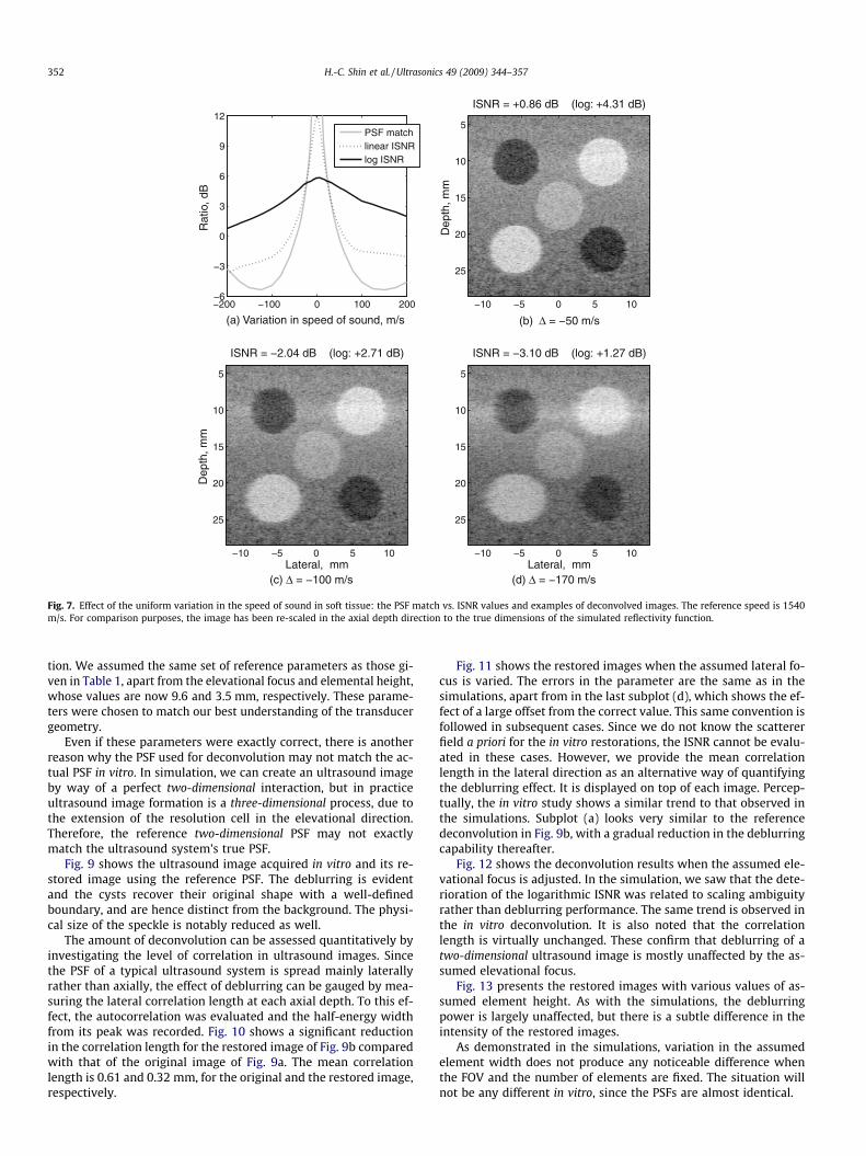
There is considerable uncertainty in the speed of sound whenscanning in vivo, both in terms of the absolute speed and its homo-geneity. In this section, however, we investigate the sensitivityonly under the assumption of an homogeneous medium. In otherwords, the speed of sound is varied uniformly throughout the tis-sue away from the nominal 1540 m/s. It is changed over the rangeof ±200 m/s.

The results in Fig. 7 are similar to those for the lateral focus inFig. 3. The logarithmic ISNR can be characterised as a single-slopecurve (�0.019 and �0.016 dB/(m/s) near the reference and aroundthe right-hand edge of the graph, respectively) and its effect on theB-scan images is one of blurring, not intensity change. Even thoughthe lateral focus of the ultrasound system is fixed, the variation inthe speed of sound will change the effective time delays betweentransducer elements, leading to different blurring characteristics.

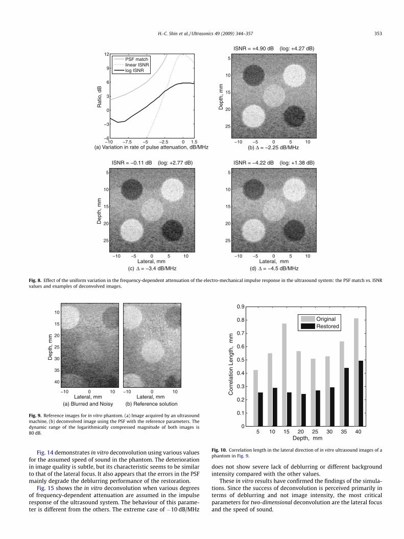
5.6. Attenuation in the electro-mechanical impulse response

Another tissue specific parameter is the frequency-dependentattenuation of the ultrasonic signal. Here, we deal with such atten-uation by adjusting the frequency spectrum of the electro-mechan-ical impulse response (henceforth, short as ‘pulse’).

In a real soft tissue environment, frequency-dependent attenu-ation occurs progressively with propagation distance. However, wesimplify the situation by applying frequency-dependent attenua-tion uniformly throughout the medium. The reference pulse wasacquired in a phantom where it could have suffered attenuationof approximately 1.5 dB/MHz. (The phantom was designed to have

0 1 2

0

3

6

9

12

(a) Variation in elemental height, mm

Rat

io, d

B


Dep

th, m

m

(b) Δ0 5 10

5

10

15

20

25

Lateral, mm

Dep

th, m

m

ISNR = +0.88 dB (log: +2.78 dB)

(c) Δ

0 5 10

5

10

15

20

25

Lateral, mm

ISNR = +1.46 dB (log: +1.25 dB)

(d) Δ

0 5 10

5

10

15

20

25

Fig. 5. Effect of the variation in the height of the transducer elements: the PSF match vs. ISNR values and examples of deconvolution images. The reference height is 6 mm.

0 10 2040

50

60

70

80

90

PS

F m

atch

, dB

Variation in width of elements, μm

PSF match

ISNR

0 10 20−20 −105

10

15

20

Line

ar IS

NR

, dB

Fig. 6. Effect of the variation in the width of the transducer elements on the PSFmatch and linear ISNR while the field-of-view and number of elements are fixed.The reference width is 170.8 lm. The decibel values for the PSF match are shown onthe left-hand side, and the linear version of the ISNR is shown on the right. Thelogarithmic version of the ISNR is not shown.

3 This is available free at http://mi.eng.cam.ac.uk/~rwp/stradwin/.


an attenuation rate of 0.4 dB/cm/MHz. The processed pulse was ac-quired for a depth of around 16 mm, which produces a round-tripattenuation of 1.3 dB/MHz.) Hence, the attenuation rate was variedfrom amplification of 1.5 dB/MHz (a hypothetically unattenuatedsignal) to the extreme case of �10 dB/MHz.

Fig. 8 shows the simulation results. In terms of perceptual eval-uation, it appears that the deblurring is not especially sensitive tothe rate of attenuation. In terms of its operating mechanism, theattenuation rate is not closely related to either beamforming orthe acoustic lens aspect of the ultrasound system. Therefore, it isconsidered to behave independently of any other parametersinvestigated in this paper.

6. Deconvolution of in vitro ultrasound images

It would appear that human perception does not demandexceptionally high accuracy from a deconvolution algorithm. Inthe previous simulation experiments, we observed negligiblechange in the perceived image quality as long as the logarithmicISNR was within �1.5 dB of the ideal solution. In some situations,a reduction in ISNR of as much as 4.5 dB was acceptable, with cor-responding PSF parameters significantly beyond the nominaluncertainty in their accuracy.

In this section, we explore whether our assessment from thesimulations is observed in more realistic ultrasound images. Thecyst region of the phantom introduced in Section 3.1 was scannedusing a clinical ultrasound system. The system consisted of a Gen-eral Electric probe RSP6-12 and a Diasus ultrasound machine fromDynamic Imaging Ltd., which was synchronised with a Gage Com-puscope CS14200 digitiser. The digitisation process was linked tothe locally-developed Stradwin software3, which is a user-friendlycross-platform tool for medical ultrasound acquisition and visualisa-

http://mi.eng.cam.ac.uk/~rwp/stradwin/

0 100 200

0

3

6

9

12

(a) Variation in speed of sound, m/s

Rat

io, d

B


Dep

th, m

m

ISNR = +0.86 dB (log: +4.31 dB)

(b) Δ0 5 10

5

10

15

20

25

Lateral, mm

Dep

th, m

m

(c) Δ

0 5 10

5

10

15

20

25

Lateral, mm(d) Δ

0 5 10

5

10

15

20

25

Fig. 7. Effect of the uniform variation in the speed of sound in soft tissue: the PSF match vs. ISNR values and examples of deconvolved images. The reference speed is 1540m/s. For comparison purposes, the image has been re-scaled in the axial depth direction to the true dimensions of the simulated reflectivity function.


tion. We assumed the same set of reference parameters as those gi-ven in Table 1, apart from the elevational focus and elemental height,whose values are now 9.6 and 3.5 mm, respectively. These parame-ters were chosen to match our best understanding of the transducergeometry.

Even if these parameters were exactly correct, there is anotherreason why the PSF used for deconvolution may not match the ac-tual PSF in vitro. In simulation, we can create an ultrasound imageby way of a perfect two-dimensional interaction, but in practiceultrasound image formation is a three-dimensional process, due tothe extension of the resolution cell in the elevational direction.Therefore, the reference two-dimensional PSF may not exactlymatch the ultrasound system’s true PSF.

Fig. 9 shows the ultrasound image acquired in vitro and its re-stored image using the reference PSF. The deblurring is evidentand the cysts recover their original shape with a well-definedboundary, and are hence distinct from the background. The physi-cal size of the speckle is notably reduced as well.

The amount of deconvolution can be assessed quantitatively byinvestigating the level of correlation in ultrasound images. Sincethe PSF of a typical ultrasound system is spread mainly laterallyrather than axially, the effect of deblurring can be gauged by mea-suring the lateral correlation length at each axial depth. To this ef-fect, the autocorrelation was evaluated and the half-energy widthfrom its peak was recorded. Fig. 10 shows a significant reductionin the correlation length for the restored image of Fig. 9b comparedwith that of the original image of Fig. 9a. The mean correlationlength is 0.61 and 0.32 mm, for the original and the restored image,respectively.

Fig. 11 shows the restored images when the assumed lateral fo-cus is varied. The errors in the parameter are the same as in thesimulations, apart from in the last subplot (d), which shows the ef-fect of a large offset from the correct value. This same convention isfollowed in subsequent cases. Since we do not know the scattererfield a priori for the in vitro restorations, the ISNR cannot be evalu-ated in these cases. However, we provide the mean correlationlength in the lateral direction as an alternative way of quantifyingthe deblurring effect. It is displayed on top of each image. Percep-tually, the in vitro study shows a similar trend to that observed inthe simulations. Subplot (a) looks very similar to the referencedeconvolution in Fig. 9b, with a gradual reduction in the deblurringcapability thereafter.

Fig. 12 shows the deconvolution results when the assumed ele-vational focus is adjusted. In the simulation, we saw that the dete-rioration of the logarithmic ISNR was related to scaling ambiguityrather than deblurring performance. The same trend is observed inthe in vitro deconvolution. It is also noted that the correlationlength is virtually unchanged. These confirm that deblurring of atwo-dimensional ultrasound image is mostly unaffected by the as-sumed elevational focus.

Fig. 13 presents the restored images with various values of as-sumed element height. As with the simulations, the deblurringpower is largely unaffected, but there is a subtle difference in theintensity of the restored images.

As demonstrated in the simulations, variation in the assumedelement width does not produce any noticeable difference whenthe FOV and the number of elements are fixed. The situation willnot be any different in vitro, since the PSFs are almost identical.

0 1.5

0

3

6

9

12

(a) Variation in rate of pulse attenuation, dB/MHz

Rat

io, d

B


Dep

th, m

m

ISNR = +4.90 dB (log: +4.27 dB)

(b) Δ0 5 10

5

10

15

20

25

Lateral, mm

Dep

th, m

m

(c) Δ

0 5 10

5

10

15

20

25

Lateral, mm(d) Δ

0 5 10

5

10

15

20

25

Fig. 8. Effect of the uniform variation in the frequency-dependent attenuation of the electro-mechanical impulse response in the ultrasound system: the PSF match vs. ISNRvalues and examples of deconvolved images.

Lateral, mm

Dep

th, m

m

(a) Blurred and Noisy

0 10

10

15

20

25

30

35

40

Lateral, mm(b) Reference solution

0 10

Fig. 9. Reference images for in vitro phantom. (a) Image acquired by an ultrasoundmachine, (b) deconvolved image using the PSF with the reference parameters. Thedynamic range of the logarithmically compressed magnitude of both images is80 dB. 5 10 15 20 25 30 35 40

0

0.1

0.2

0.3

0.4

0.5

0.6

0.7

0.8

0.9

Depth, mm

Cor

rela

tion

Leng

th,

mm

OriginalRestored

Fig. 10. Correlation length in the lateral direction of in vitro ultrasound images of aphantom in Fig. 9.


Fig. 14 demonstrates in vitro deconvolution using various valuesfor the assumed speed of sound in the phantom. The deteriorationin image quality is subtle, but its characteristic seems to be similarto that of the lateral focus. It also appears that the errors in the PSFmainly degrade the deblurring performance of the restoration.

Fig. 15 shows the in vitro deconvolution when various degreesof frequency-dependent attenuation are assumed in the impulseresponse of the ultrasound system. The behaviour of this parame-ter is different from the others. The extreme case of �10 dB/MHz

does not show severe lack of deblurring or different backgroundintensity compared with the other values.

These in vitro results have confirmed the findings of the simula-tions. Since the success of deconvolution is perceived primarily interms of deblurring and not image intensity, the most criticalparameters for two-dimensional deconvolution are the lateral focusand the speed of sound.

Lateral, mm

Dep

th, m

m

(a) Δ = +2 mm

corr. = 0.32 mm

0 5 10

10

15

20

25

30

35

40

Lateral, mm(b) Δ = +4.5 mm

Lateral Focuscorr. = 0.49 mm

0 5 10Lateral, mm

(c) Δ = +8 mm

corr. = 0.65 mm

0 5 10Lateral, mm

(d) Δ = +12 mm

corr. = 0.82 mm

0 5 10

Fig. 11. Examples of deconvolved images and their mean correlation length for the in vitro phantom with the variation in the axial depth of the lateral focus. The referencefocal depth is 16 mm. The dynamic range of the logarithmically compressed magnitude of the images is 80 dB. The title of each image shows its mean correlation length in thelateral direction, and those of the original ultrasound image and the reference deconvolution are 0.61 and 0.32 mm, respectively.

Lateral, mm

Dep

th, m

m

(a) Δ = +0.615 mm

corr. = 0.32 mm

0 5 10

10

15

20

25

30

35

40

Lateral, mm(b) Δ = +1.3 mm

Elevational Focuscorr. = 0.32 mm

0 5 10Lateral, mm

(c) Δ = +2.5 mm

corr. = 0.32 mm

0 5 10Lateral, mm

(d) Δ = +12 mm

corr. = 0.33 mm

0 5 10

Fig. 12. Examples of deconvolved images and their mean correlation length for the in vitro phantom with varying values of the radius of the elevational focus. The referencefocal radius is 9.6 mm.

Lateral, mm

Dep

th, m

m

(a) Δ

corr. = 0.32 mm

0 5 10

10

15

20

25

30

35

40

Lateral, mm(b) Δ

Height of Elementscorr. = 0.32 mm

0 5 10Lateral, mm

(c) Δ

corr. = 0.36 mm

0 5 10Lateral, mm

(d) Δ

corr. = 0.39 mm

0 5 10

Fig. 13. Examples of deconvolved images and their mean correlation length for the in vitro phantom for various values of the height of the transducer elements. The referenceheight is 3.5 mm.


Lateral, mm

Dep

th, m

m

(a) Δ

corr. = 0.33 mm

0 5 10

10

15

20

25

30

35

40

Lateral, mm(b) Δ

Speed of Soundcorr. = 0.34 mm

0 5 10Lateral, mm

(c) Δ

corr. = 0.37 mm

0 5 10Lateral, mm

(d) Δ

corr. = 0.40 mm

0 5 10

Fig. 14. Examples of deconvolved images and their mean correlation length for the in vitro phantom for various values of the speed of sound in soft tissue. The reference speedis 1540 m/s. For comparison purpose, the image has been re-scaled in the axial depth direction to the true dimensions of the designed phantom (that was scanned).

Lateral, mm

Dep

th,

mm

(a) Δ

corr. = 0.34 mm

0 5 10

10

15

20

25

30

35

40

Lateral, mm(b) Δ

Pulse Attenuationcorr. = 0.35 mm

0 5 10Lateral, mm

(c) Δ

corr. = 0.37 mm

0 5 10Lateral, mm

(d) Δ

corr. = 0.43 mm

0 5 10

Fig. 15. Examples of deconvolved images and their mean correlation length for the in vitro phantom assuming various degrees of frequency-dependent attenuation in theelectro-mechanical impulse response.

Lateral, mm

Dep

th,

mm

(a) Blurred and Noisy

0 5 10

10

15

20

25

30

Lateral, mm

(b) Deconvolution

0 5 10

Fig. 16. Ultrasound images for in vivo forearm. (a) Image acquired by an ultrasound machine, (b) restored image using the PSF with the reference parameters. The dynamicrange of the logarithmically compressed magnitude of the images is 80 dB.


5 10 15 20 25 300

0.1

0.2

0.3

0.4

0.5

0.6

0.7

0.8

0.9

Depth, mm

Cor

rela

tion

Leng

th, m

m

OriginalRestored

Fig. 17. Correlation length in the lateral direction of in vivo ultrasound images of aforearm in Fig. 16.


7. Deconvolution of in vivo ultrasound image

In this section, we apply our deconvolution algorithm in vivo.The same clinical ultrasound system as was used for the in vitroacquisition was also used to scan a left forearm, near the elbow.Fig. 16 shows the acquired ultrasound image and its restored ver-sion using the PSF used for the reference deconvolution of in vitroimages.

We expect the discrepancy between reference and true param-eters to get even worse in vivo, the most significant reason beingthe inhomogeneous composition of soft tissue. Nonetheless, thedeconvolution result illustrates the robustness of our restorationmethod to such potential errors and its applicability in vivo. Thephysical size of the speckle is reduced and deblurring is evident,especially in the dominant curved feature.

The lateral correlation lengths for the in vivo images are shownin Fig. 17. The reduction is consistent at all depths, though not as

0 0.25 0.5 0.75 1 1.25 −1

−0.5

0

0.5

1

Time, μs

Nor

mal

ised

Am

plitu

de

Fig. 18. Example waveform of an electro-mechanical impulse response taken by aGeneral Electric RSP6-12 probe operated by Diasus ultrasound system fromDynamic Imaging Ltd.

significant as the in vitro case: this is unsurprising given the likelydiscrepancy between the assumed and the actual PSF in vivo. Themean correlation length is 0.55 mm in the original image and0.42 mm in the restored image.

8. Conclusions

In the simulations, we observed that the quantitative differencein deconvolution in terms of the linear version of the ISNR was sim-ilar to that derived from measuring changes directly in the PSF. Weconclude that the ISNR measure based on the logarithmic imageamplitude is a better indicator of the perceived improvement inthe restored ultrasound images.

Simulation and in vitro studies showed that, in terms of effec-tive deblurring in a two-dimensional restoration, the two mostinfluential parameters are the axial depth of the lateral focus andthe speed of sound in soft tissue. The other parameters principallyadjust the intensity level of the restored image, but do not makesignificant differences to deblurring.

Based on these perceptual judgements, assisted by the logarith-mic ISNR metric, it was concluded that we could estimate a PSFwith acceptable accuracy producing a deconvolution with im-proved image quality. Therefore, we were also able to demonstratethat even in vivo ultrasound images could be restored despiteassumptions based on unknown parameters of the ultrasound sys-tem and the soft tissue under examination.

Acknowledgements

The work was funded by the Engineering and Physical SciencesResearch Council (reference EP/E007112/1) in the United Kingdom.

Appendix A. Estimation of electro-mechanical impulse response

In this appendix, we briefly describe how the electro-mechani-cal impulse response (henceforth, referred to as the ‘pulse’) may beestimated using a parametric method based on acquired backscat-tered RF data.

The use of parametric methods to estimate the shape of theultrasound pulse was proposed by Jensen [15]. His method as-sumes an ARMA (auto-regressive moving average) model and theparameters are estimated using acquired A-line data by an itera-tive gradient-search scheme. Here, however, we discuss the taskof estimating the same pulse more simply by using an AR (auto-regressive) model. It is well known that an ARMA model can beapproximated by an AR model of sufficiently high order, and ARmodels may be preferred because their parameters are much easierto estimate.

Parametric methods assume that the observed trace may berepresented as the result of filtering a white noise process. If thewhite noise process is considered to be a random spike series, thenthis assumption is equivalent to saying that the observed trace isobtained by convolving the underlying pulse onto this spike series[16]. For a region characterised by uniform weak scattering, thisappears to be a reasonable assumption to make since the scattererswithin the region behave approximately like spikes, randomlyspaced and with random scattering strengths.

AR modelling represents the underlying pulse as an all-pole fil-ter. Let the digitised samples of an observed trace be g(n), the whitenoise process be e(n) and the digitised samples of the pulse be v(n).The corresponding z-transforms are denoted by G(z), E(z), and V(z),respectively. The filtering operation may be expressed as,

GðzÞ ¼ EðzÞVðzÞ ) GðzÞEðzÞ ¼ VðzÞ ¼ 1

1þPM

m¼1amz�mðA:1Þ


where am is the sequence of filter coefficients that need to be deter-mined to obtain v(n), and M is the order of the AR process. This z-domain equation may also be expressed in the more familiar formof a difference equation:

gðnÞ þXM

m¼1

amgðn�mÞ ¼ eðnÞ ðA:2Þ

The sequence am may be estimated by minimising the error in theleast squares sense, for example using the Yule–Walker or normalequation. This procedure is also known in the domain of predictivedeconvolution [16] or forward linear prediction [14].

To recover the underlying pulse v(n), the discrete-time Fouriertransform V(ejx) of v(n) can be computed from Eq. (A.1) with thesubstitution z = ejx. The inverse Fourier transform is then appliedto V(ejx). We then assumed a minimum phase for the pulse shape.Fig. 18 shows an example of an electro-mechanical impulseresponse estimated by the method outlined here. It is usedthroughout this paper and acted as the reference pulse when fre-quency-dependent attenuation was applied.

References

[1] Z.-H. Cho, J.P. Jones, M. Singh, Foundations of Medical Imaging, John Wiley &Sons, Inc, New York, 1993 (Chapter 15. Ultrasonic Imaging, pp. 521–548).

[2] P. Suetens, Fundamentals of Medical Imaging, Cambridge University Press,Cambridge, UK, 2002 (Chapter 7. Ultrasonic Imaging, pp. 90–146).

[3] T.L. Szabo, Diagnostic Ultrasound Imaging: Inside Out, Elsevier Academic Press,Amsterdam, 2004 (Chapter 10. Imaging Systems and Applications, pp. 297–336).

[4] J. Ng, R. Prager, N. Kingsbury, G. Treece, A. Gee, Modeling ultrasound imagingas a linear shift-variant system, IEEE Transactions on Ultrasonics,Ferroelectrics, and Frequency Control 53 (3) (2006) 549–563.

[5] J. Ng, R. Prager, N. Kingsbury, G. Treece, A. Gee, Wavelet restoration of medicalpulse-echo ultrasound images in an EM framework, IEEE Transactions onUltrasonics, Ferroelectrics, and Frequency Control 54 (3) (2007)550–568.

[6] J. Ng, H. Gomersall, R. Prager, N. Kingsbury, G. Treece, A. Gee, Waveletrestoration of three-dimensional medical pulse-echo ultrasound datasets in anEM framework, in: Proceedings of the 29th International Symposium onAcoustical Imaging, Shonan, Kanagawa, Japan, 2007.

[7] C.W. Therrien, Discrete Random Signals and Statistical Signal Processing,Prentice Hall, Inc, Englewood Ciffs, NJ, USA, 1992.

[8] N. Kingsbury, Image processing with complex wavelets, PhilosophicalTransactions of The Royal Society of London Series A 357 (1999) 2543–2560.

[9] N. Kingsbury, Complex wavelets for shift invariant analysis and filtering ofsignals, Applied and Computational Harmonic Analysis 10 (2001) 234–253.

[10] L. Sendur, I.W. Selesnick, Bivariate shrinkage functions for wavelet-baseddenoising exploiting interscale dependency, IEEE Transactions on SignalProcessing 50 (11) (2002) 2744–2756.

[11] J. Jensen, N.B. Svendsen, Calculation of pressure fields from arbitrarily shaped,apodized, and excited ultrasound transducers, IEEE Transactions onUltrasonics, Ferroelectrics, and Frequency Control 39 (1992) 262–267.

[12] J. Jensen, Field: A program for simulating ultrasound systems, Medical &Biological Engineering & Computing 34 (1996) 351–353 (Presented at the 10thNordic–Baltic Conference on Biomedical Imaging).

[13] J.C. Bamber, R.J. Dickinson, Ultrasonic B-scanning: a computer simulation,Physics in Medicine and Biology 25 (3) (1980) 463–479.

[14] J.G. Proakis, G.M. Dimitris, Digital Signal Processing: Principles, Algorithms,and Application, third ed., Prentice-Hall, London, 1996 (Chapter 11. LinearPrediction and Optimum Linear Filters, pp. 852–895).

[15] J.A. Jensen, Estimation of pulses in ultrasound B-scan images, IEEETransactions on Medical Imaging 10 (2) (1991) 164–172.

[16] E.A. Robinson, S. Treitel, Applications of Digital Signal Processing, Prentice-Hall, Signal Processing Series, Springer, 1978 (Chapter 7. Digital SignalProcessing in Geophysics, pp. 439–491).

Sensitivity to point-spread function parameters in medical ultrasound image deconvolution

Documents

Transcript of Sensitivity to point-spread function parameters in medical ultrasound image deconvolution