from numerical optimization strategies to blind deconvolution ...
175
HAL Id: tel-01764912 https://tel.archives-ouvertes.fr/tel-01764912 Submitted on 12 Apr 2018 HAL is a multi-disciplinary open access archive for the deposit and dissemination of sci- entific research documents, whether they are pub- lished or not. The documents may come from teaching and research institutions in France or abroad, or from public or private research centers. L’archive ouverte pluridisciplinaire HAL, est destinée au dépôt et à la diffusion de documents scientifiques de niveau recherche, publiés ou non, émanant des établissements d’enseignement et de recherche français ou étrangers, des laboratoires publics ou privés. Contributions to image restoration : from numerical optimization strategies to blind deconvolution and shift-variant deblurring Rahul Kumar Mourya To cite this version: Rahul Kumar Mourya. Contributions to image restoration : from numerical optimization strategies to blind deconvolution and shift-variant deblurring. Signal and Image processing. Université de Lyon, 2016. English. NNT : 2016LYSES005. tel-01764912
-
Upload
khangminh22 -
Category
Documents
-
view
0 -
download
0
Transcript of from numerical optimization strategies to blind deconvolution ...

HAL Id: tel-01764912https://tel.archives-ouvertes.fr/tel-01764912
Submitted on 12 Apr 2018
HAL is a multi-disciplinary open accessarchive for the deposit and dissemination of sci-entific research documents, whether they are pub-lished or not. The documents may come fromteaching and research institutions in France orabroad, or from public or private research centers.
L’archive ouverte pluridisciplinaire HAL, estdestinée au dépôt et à la diffusion de documentsscientifiques de niveau recherche, publiés ou non,émanant des établissements d’enseignement et derecherche français ou étrangers, des laboratoirespublics ou privés.
Contributions to image restoration : from numericaloptimization strategies to blind deconvolution and
shift-variant deblurringRahul Kumar Mourya
To cite this version:Rahul Kumar Mourya. Contributions to image restoration : from numerical optimization strategiesto blind deconvolution and shift-variant deblurring. Signal and Image processing. Université de Lyon,2016. English. NNT : 2016LYSES005. tel-01764912
N d’ordre xxxx Année 2016Thèse
Contributions to Image Restoration:From Numerical Optimization Strategies
to Blind Deconvolution and Shift-variant DeblurringContributions pour la restauration d’images:
des stratégies d’optimisation numérique à la déconvolutionaveugle et à la correction de flous spatialement variables
présentée le 1er Février 2016à lÉcole Doctorale Science Ingénierie SantéProgramme doctoral en Image Vision Signal
Faculté des Sciences et Techniques
Université Jean Monnet, Saint-Etiennepour l’obtention du grade de Docteur ès Sciences
par
Rahul Kumar MOURYA
acceptée sur proposition du jury:
M. Hervé CARFANTAN, Maître de Conférences à l’Université Paul Sabatier, rapporteurMme. Emilie CHOUZENOUX, Maître de Conférences à l’Université Paris-Est, examinatrice
M. Frederic DIAZ, Ingénieur de recherche à Thales Angénieux, invitéM. Paulo GONCALVES,Directeur de Recherche à l’INRIA, examinateurM. François GOUDAIL, Professeur à l’Institut d’Optique, examinateurM. Laurent MUGNIER, Maître de Recherche à l’ONERA, rapporteur
M. Jean-Marie BECKER, Professeur à CPE Lyon, directeur de thèseM. Eric THIEBAUT, Astronome Adjoint à l’Université Lyon 1, co-encadrant
M. Loïc DENIS, Maître de Conférences à l’Université Jean Monnet, co-encadrant
Laboratoire Hubert Curien UMR-CNRS 5516Saint-Etienne
UMR • CNRS • 5516 • SAINT-ETIENNE


It is not knowledge, but the act of learning,not possession but the act of getting there,
which grants the greatest enjoyment.— Carl Friedrich Gauss
Dedicated to my parents Usha Mourya and Gobardhan Mourya.

iii
Abstract
Degradations of images during the acquisition process is inevitable; images suffer fromblur and noise. With advances in technologies and computational tools, the degradationsin the images can be avoided or corrected up to a significant level, however, the quality ofacquired images is still not adequate for many applications. This calls for the developmentof more sophisticated digital image restoration tools. This thesis is a contribution to imagerestoration.
The thesis is divided into five chapters, each including a detailed discussion on differ-ent aspects of image restoration. It starts with a generic overview of imaging systems, andpoints out the possible degradations occurring in images with their fundamental causes.In some cases the blur can be considered stationary throughout the field-of-view, and thenit can be simply modeled as convolution. However, in many practical cases, the blur variesthroughout the field-of-view, and thus modeling the blur is not simple considering the ac-curacy and the computational effort. The first part of this thesis presents a detailed discus-sion on modeling of shift-variant blur and its fast approximations, and then it describesa generic image formation model. Subsequently, the thesis shows how an image restora-tion problem, can be seen as a Bayesian inference problem, and then how it turns into alarge-scale numerical optimization problem. Thus, the second part of the thesis considersa generic optimization problem that is applicable to many domains, and then proposes aclass of new optimization algorithms for solving inverse problems in imaging. The pro-posed algorithms are as fast as the state-of-the-art algorithms (verified by several numer-ical experiments), but without any hassle of parameter tuning, which is a great relief forusers.
The third part of the thesis presents an in depth discussion on the shift-invariant blindimage deblurring problem suggesting different ways to reduce the ill-posedness of theproblem, and then proposes a blind image deblurring method using an image decom-position for restoration of astronomical images. The proposed method is based on analternating estimation approach. The restoration results on synthetic astronomical scenesare promising, suggesting that the proposed method is a good candidate for astronomicalapplications after certain modifications and improvements. The last part of the thesis ex-tends the ideas of the shift-variant blur model presented in the first part. This part gives adetailed description of a flexible approximation of shift-variant blur with its implementa-tional aspects and computational cost. This part presents a shift-variant image deblurringmethod with some illustrations on synthetically blurred images, and then it shows howthe characteristics of shift-variant blur due to optical aberrations can be exploited for PSFestimation methods. This part describes a PSF calibration method for a simple experi-mental camera suffering from optical aberration, and then shows results on shift-variantimage deblurring of the images captured by the same experimental camera. The resultsare promising, and suggest that the two steps can be used to achieve shift-variant blindimage deblurring, the long-term goal of this thesis. The thesis ends with the conclusionsand suggestions for future works in continuation of the current work.

v
Résumé
L’introduction de dégradations lors du processus de formation d’images est unphénomène inévitable: les images souffrent de flou et de la présence de bruit. Avec lesprogrès technologiques et les outils numériques, ces dégradations peuvent être compen-sées jusqu’à un certain point. Cependant, la qualité des images acquises est insuffisantepour de nombreuses applications. Cette thèse contribue au domaine de la restaurationd’images.
La thèse est divisée en cinq chapitres, chacun incluant une discussion détaillée surdifférents aspects de la restauration d’images. La thèse commence par une présentationgénérale des systèmes d’imagerie et pointe les dégradations qui peuvent survenir ainsi queleurs origines. Dans certains cas, le flou peut être considéré stationnaire dans tout le champde vue et est alors simplement modélisé par un produit de convolution. Néanmoins, dansde nombreux cas de figure, le flou est spatialement variable et sa modélisation est plusdifficile, un compromis devant être réalisé entre la précision de modélisation et la com-plexité calculatoire. La première partie de la thèse présente une discussion détaillée sur lamodélisation des flous spatialement variables et différentes approximations efficaces per-mettant de les simuler. Elle décrit ensuite un modèle de formation de l’image générique.Puis, la thèse montre que la restauration d’images peut s’interpréter comme un problèmed’inférence bayésienne et ainsi être reformulé en un problème d’optimisation en grandedimension. La deuxième partie de la thèse considère alors la résolution de problèmesd’optimisation génériques, en grande dimension, tels que rencontrés dans de nombreuxdomaines applicatifs. Une nouvelle classe de méthodes d’optimisation est proposée pourla résolution des problèmes inverses en imagerie. Les algorithmes proposés sont aussirapides que l’état de l’art (d’après plusieurs comparaisons expérimentales) tout en sup-primant la difficulté du réglage de paramètres propres à l’algorithme d’optimisation, cequi est particulièrement utile pour les utilisateurs. La troisième partie de la thèse traite duproblème de la déconvolution aveugle (estimation conjointe d’un flou invariant et d’uneimage plus nette) et suggère différentes façons de contraindre ce problème d’estimation.Une méthode de déconvolution aveugle adaptée à la restauration d’images astronomiquesest développée. Elle se base sur une décomposition de l’image en sources ponctuelles etsources étendues et alterne des étapes de restauration de l’image et d’estimation du flou.Les résultats obtenus en simulation suggèrent que la méthode peut être un bon point dedépart pour le développement de traitements dédiés à l’astronomie. La dernière partiede la thèse étend les modèles de flous spatialement variables pour leur mise en œuvrepratique. Une méthode d’estimation du flou est proposée dans une étape d’étalonnage.Elle est appliquée à un système expérimental, démontrant qu’il est possible d’imposer descontraintes de régularité et d’invariance lors de l’estimation du flou. L’inversion du flouestimé permet ensuite d’améliorer significativement la qualité des images. Les deux étapesd’estimation du flou et de restauration forment les deux briques indispensables pour met-tre en œuvre, à l’avenir, une méthode de restauration aveugle (c’est à dire, sans étalonnagepréalable). La thèse se termine par une conclusion ouvrant des perspectives qui pourrontêtre abordées lors de travaux futurs.

vii
Acknowledgements
This thesis would not have been successful without the great contributions from differ-ent people. Foremost, I express my sincere gratitude to my three advisors Loïc DENIS,Asst.Prof. at University of Saint-Etienne, Éric THIÉBAUT, Astronomer at Observatory ofLyon, and Jean-Marie BECKER, Prof. at CPE Lyon, for their continuous support, patience,motivation, enthusiasm, and immense knowledge during the whole PhD study and re-search. Their guidance helped me during all the time of the research and the writing ofthis thesis. I must admit that I am very lucky to have them as advisors and mentors formy thesis.
Besides my advisors, I am grateful to the reviewers of my thesis, Laurent MUGNIER,senior research scientist at ONERA, and Hervé CARFANTAN, Asst. Prof. at Universityof Toulouse, for their comments and advices in the report, which helped to improved thequality of my presentation for the defense day and the final draft of the thesis.
Moreover, I express my gratitude to the other jury members: Emilie CHOUZENOUX,Asst. Prof. at University of Paris East, Paolo GONCALVES, director of research at INRIA,François GOUDAIL, Prof. at Institute of Optics, ParisTech, and Frederic DIAZ, researchengineer at Thales Angénieux, for their questions and suggestions on the defense day.
I am also very thankful to different faculty members at University of Saint-Etienne andresearchers at Laboratory Hubert Curien for their suggestions and helps during the wholetenure of my PhD and Master studies. Some of them I would like to mention here areCorinne FOURNIER, Asst. Prof., Thierry LEPINE, Asst. Prof, Thierry FOURNEL, Prof.,Olivier ALATA, Prof., Marc SEBBAN, Prof., Amaury HABRARD, Prof., Elisa FROMONT,Asst. Prof., Éric DINET, Asst.Prof., and Damien MUSELET, Asst. Prof. I want to expressdeep gratitude to Alain TRÉMEAU, Prof. for his all supports and suggestions from thebeginning of my Master studies till the completion of my PhD.
I am also very grateful to had have very helpful colleagues and friends around me,some of them I would like to mention here are Rahat Khan, Abul Hasnat, Moham-mad Nawaf, Praveen Velpula, Chiranjeevi Maddi, Emile Bevillon, Ciro Damico, DiegoFrancesca, Chiara Cangialosi, Serena Rizzolo, Adriana Morana, Alina Toma, NataliaNeverova, Mohamed Elawady, Raad Deep, Carlos Arango, and Ar-pha Pisanpeeti.
Moreover, I want to acknowledge the Région Rhône Alpes (ARC6) for fully fundingmy PhD studies.
Last but not least, I want to thank all the members in administration working at theLaboratory Hubert Curien and University of Saint-Etienne for their help during my PhDstudies.
Saint-Etienne, 1st Feb 2016 Rahul Mourya

Contents
Abstract iii
Résumé v
Acknowledgements vii
List of Figures xiv
List of Tables xviii
Résumé des chapitres xix
1 An Introduction to Image Restoration: From Blur Models to Restoration Methods 31.1 Introduction . . . . . . . . . . . . . . . . . . . . . . . . . . . . . . . . . . . . . 41.2 A Brief Introduction to Imaging Systems . . . . . . . . . . . . . . . . . . . . . 51.3 Modeling the Blur Degradation and its Approximations . . . . . . . . . . . . 8
1.3.1 Shift-Invariant Blur . . . . . . . . . . . . . . . . . . . . . . . . . . . . . 101.3.2 Shift-Variant Blur . . . . . . . . . . . . . . . . . . . . . . . . . . . . . . 11
1.4 Noise in the Image Acquisition Process . . . . . . . . . . . . . . . . . . . . . 181.5 Image Restoration . . . . . . . . . . . . . . . . . . . . . . . . . . . . . . . . . . 181.6 Bayesian Inference Framework for Image Restoration . . . . . . . . . . . . . 20
1.6.1 Image Restoration Strategies . . . . . . . . . . . . . . . . . . . . . . . 211.7 Observation Models . . . . . . . . . . . . . . . . . . . . . . . . . . . . . . . . 231.8 Image and PSF Prior Models . . . . . . . . . . . . . . . . . . . . . . . . . . . . 25
1.8.1 Role of Hyperparameters and their Estimation . . . . . . . . . . . . . 271.9 Our Approach to Blind Image Deblurring . . . . . . . . . . . . . . . . . . . . 271.10 Outline of the Thesis and Contributions . . . . . . . . . . . . . . . . . . . . . 28
2 A Nonsmooth Optimization Strategy for Inverse Problems in Imaging 312.1 Introduction . . . . . . . . . . . . . . . . . . . . . . . . . . . . . . . . . . . . . 32
2.1.1 Recall of Notations and Some Convex Optimization Properties . . . 332.2 Relevant Existing Approaches . . . . . . . . . . . . . . . . . . . . . . . . . . . 362.3 Proposed Algorithm . . . . . . . . . . . . . . . . . . . . . . . . . . . . . . . . 41
2.3.1 Motivation and Contributions . . . . . . . . . . . . . . . . . . . . . . 412.3.2 Basic Ingredients . . . . . . . . . . . . . . . . . . . . . . . . . . . . . . 432.3.3 Derivation of the Algorithm . . . . . . . . . . . . . . . . . . . . . . . . 452.3.4 The Proposed Algorithm: ALBHO . . . . . . . . . . . . . . . . . . . . 46
2.4 Comparison of ALBHO with State-Of-The-Art Algorithms . . . . . . . . . . 472.4.1 Problem 1: Image Deblurring with TV and Positivity Constraint . . . 472.4.2 Problem 2: Poissonian Image Deblurring with TV and Positivity
Constraint . . . . . . . . . . . . . . . . . . . . . . . . . . . . . . . . . . 50
x Contents
2.4.3 Problem 3: Image Segmentation . . . . . . . . . . . . . . . . . . . . . 522.4.4 Performance Comparison of Proximal Newton-type Method vs.
ADMM vs. ALBHO . . . . . . . . . . . . . . . . . . . . . . . . . . . . 532.4.5 Computational Cost of the Algorithms . . . . . . . . . . . . . . . . . 56
2.5 Numerical Experiments and Results . . . . . . . . . . . . . . . . . . . . . . . 572.5.1 Experimental Setup . . . . . . . . . . . . . . . . . . . . . . . . . . . . . 572.5.2 Performance Comparison of the Algorithms . . . . . . . . . . . . . . 582.5.3 Analysis of Results . . . . . . . . . . . . . . . . . . . . . . . . . . . . . 59
2.6 Conclusions . . . . . . . . . . . . . . . . . . . . . . . . . . . . . . . . . . . . . 702.7 Summary . . . . . . . . . . . . . . . . . . . . . . . . . . . . . . . . . . . . . . . 70
3 Image Decomposition Approach for Image Restoration 713.1 Introduction . . . . . . . . . . . . . . . . . . . . . . . . . . . . . . . . . . . . . 723.2 Signal Decomposition Approaches . . . . . . . . . . . . . . . . . . . . . . . . 733.3 An Approach Toward Astronomical Image Restoration via Image Decom-
position and Blind Image Deblurring . . . . . . . . . . . . . . . . . . . . . . . 763.3.1 Introduction . . . . . . . . . . . . . . . . . . . . . . . . . . . . . . . . . 763.3.2 The Objective and The Proposed Approach . . . . . . . . . . . . . . . 773.3.3 The Likelihood and The Priors . . . . . . . . . . . . . . . . . . . . . . 783.3.4 Blind Image Deblurring as a Constrained Minimization Problem . . 803.3.5 Selection of Hyperparameters . . . . . . . . . . . . . . . . . . . . . . . 823.3.6 Experiments and Results . . . . . . . . . . . . . . . . . . . . . . . . . . 833.3.7 Analysis of Results . . . . . . . . . . . . . . . . . . . . . . . . . . . . . 83
3.4 Conclusion and Perspective . . . . . . . . . . . . . . . . . . . . . . . . . . . . 973.5 Summary . . . . . . . . . . . . . . . . . . . . . . . . . . . . . . . . . . . . . . . 98
4 Restoration of Images with Shift-Variant Blur 994.1 Introduction . . . . . . . . . . . . . . . . . . . . . . . . . . . . . . . . . . . . . 1004.2 Implementation and Cost Complexity Details of Shift-Variant Blur Operator 1014.3 Shift-Variant Image Deblurring . . . . . . . . . . . . . . . . . . . . . . . . . . 1054.4 Estimation of Shift-Variant Blur . . . . . . . . . . . . . . . . . . . . . . . . . . 107
4.4.1 Characteristics of Blur due to Optical Aberrations . . . . . . . . . . . 1074.4.2 Estimation of Shift-Variant Blur due to Optical Aberrations . . . . . . 1094.4.3 Shift-Variant PSFs Calibration . . . . . . . . . . . . . . . . . . . . . . . 111
4.5 Conclusion . . . . . . . . . . . . . . . . . . . . . . . . . . . . . . . . . . . . . . 1134.6 Summary . . . . . . . . . . . . . . . . . . . . . . . . . . . . . . . . . . . . . . . 114
5 Conclusions and Future Works 1215.1 Discussion and Conclusion . . . . . . . . . . . . . . . . . . . . . . . . . . . . 1215.2 Future Work . . . . . . . . . . . . . . . . . . . . . . . . . . . . . . . . . . . . . 123
6 Conclusion et travaux futurs 1256.1 Discussion et Conclusion . . . . . . . . . . . . . . . . . . . . . . . . . . . . . . 1256.2 Travaux futurs . . . . . . . . . . . . . . . . . . . . . . . . . . . . . . . . . . . . 127
A Appendix 129A.1 Functional Analysis . . . . . . . . . . . . . . . . . . . . . . . . . . . . . . . . . 129
A.1.1 Definitions . . . . . . . . . . . . . . . . . . . . . . . . . . . . . . . . . . 129A.2 Solution to TV -G and TV -E image decomposition models . . . . . . . . . . 131
A.2.1 Image Denoising by TV -E Model . . . . . . . . . . . . . . . . . . . . 131A.2.2 Image Deblurring via TV -E model . . . . . . . . . . . . . . . . . . . . 135

Contents xi
Bibliography 141
Table des matières
1 Une introduction à la restauration d’images: des modèles de flou aux méthodesde restauration 31.1 Introduction . . . . . . . . . . . . . . . . . . . . . . . . . . . . . . . . . . . . 41.2 Une brève introduction aux systèmes d’imagerie . . . . . . . . . . . . . . . 51.3 Modélisation et approximation du flou . . . . . . . . . . . . . . . . . . . . . 8
1.3.1 Flou stationnaire . . . . . . . . . . . . . . . . . . . . . . . . . . . . . . 101.3.2 Flou non stationnaire . . . . . . . . . . . . . . . . . . . . . . . . . . . . 11
1.4 Bruit lors de l’acquisition de l’image . . . . . . . . . . . . . . . . . . . . . . 181.5 Restauration d’images . . . . . . . . . . . . . . . . . . . . . . . . . . . . . . . 181.6 Le cadre bayésien pour la restauration d’images . . . . . . . . . . . . . . . . 20
1.6.1 Stratégies de restauration . . . . . . . . . . . . . . . . . . . . . . . . . 211.7 Modèles d’observation . . . . . . . . . . . . . . . . . . . . . . . . . . . . . . 231.8 Modèles a priori d’images et de PSF . . . . . . . . . . . . . . . . . . . . . . . 25
1.8.1 Rôle et estimation des hyper-paramètres . . . . . . . . . . . . . . . . . 271.9 Approche retenue pour la restauration aveugle . . . . . . . . . . . . . . . . 271.10 Structure de la thèse et contributions . . . . . . . . . . . . . . . . . . . . . . 28
2 Une stratégie d’optimisation non lisse pour les problèmes inverses en imagerie 312.1 Introduction . . . . . . . . . . . . . . . . . . . . . . . . . . . . . . . . . . . . 32
2.1.1 Rappels de notations et d’optimisation convexe . . . . . . . . . . . . . 332.2 Approches existantes . . . . . . . . . . . . . . . . . . . . . . . . . . . . . . . 362.3 Algorithme proposé . . . . . . . . . . . . . . . . . . . . . . . . . . . . . . . . 41
2.3.1 Motivation et Contributions . . . . . . . . . . . . . . . . . . . . . . . . 412.3.2 Briques de base . . . . . . . . . . . . . . . . . . . . . . . . . . . . . . . 432.3.3 Présentation de l’algorithme . . . . . . . . . . . . . . . . . . . . . . . . 452.3.4 L’algorithme proposé: ALBHO . . . . . . . . . . . . . . . . . . . . . . 46
2.4 Comparaison d’ALBHO à l’état de l’art . . . . . . . . . . . . . . . . . . . . . 472.4.1 Problème 1: Défloutage d’images avec contraintes de positivité et
variation totale . . . . . . . . . . . . . . . . . . . . . . . . . . . . . . . 472.4.2 Problème 2: Défloutage d’images sous un bruit poissonnien . . . . . 502.4.3 Problème 3: Segmentation d’image . . . . . . . . . . . . . . . . . . . . 522.4.4 Comparaison de performance: Proximal Newton-type vs ADMM vs
ALBHO . . . . . . . . . . . . . . . . . . . . . . . . . . . . . . . . . . . 532.4.5 Coût calculatoire des algorithmes . . . . . . . . . . . . . . . . . . . . . 56
2.5 Expériences numériques et résultats . . . . . . . . . . . . . . . . . . . . . . . 572.5.1 Cadre expérimental . . . . . . . . . . . . . . . . . . . . . . . . . . . . . 572.5.2 Comparaison de performance des algorithmes . . . . . . . . . . . . . 582.5.3 Analyse des résultats . . . . . . . . . . . . . . . . . . . . . . . . . . . . 59
2.6 Conclusions . . . . . . . . . . . . . . . . . . . . . . . . . . . . . . . . . . . . . 70

Table des matières xiii
2.7 Résumé . . . . . . . . . . . . . . . . . . . . . . . . . . . . . . . . . . . . . . . 70
3 Une approche de type “décomposition d’images” pour la restauration 713.1 Introduction . . . . . . . . . . . . . . . . . . . . . . . . . . . . . . . . . . . . 723.2 Approches de décomposition de signaux . . . . . . . . . . . . . . . . . . . . 733.3 Une approche de déconvolution aveugle basée sur la décomposition
d’images pour la restauration d’images astronomiques . . . . . . . . . . . . 763.3.1 Introduction . . . . . . . . . . . . . . . . . . . . . . . . . . . . . . . . . 763.3.2 Objectif et méthode proposée . . . . . . . . . . . . . . . . . . . . . . . 773.3.3 Vraisemblance et a priori . . . . . . . . . . . . . . . . . . . . . . . . . . 783.3.4 Formulation de la déconvolution aveugle comme un problème
d’optimisation sous contrainte . . . . . . . . . . . . . . . . . . . . . . 803.3.5 Choix des hyper-paramètres . . . . . . . . . . . . . . . . . . . . . . . . 823.3.6 Expériences et résultats . . . . . . . . . . . . . . . . . . . . . . . . . . . 833.3.7 Analyse des résultats . . . . . . . . . . . . . . . . . . . . . . . . . . . . 83
3.4 Conclusion et perspectives . . . . . . . . . . . . . . . . . . . . . . . . . . . . 973.5 Résumé . . . . . . . . . . . . . . . . . . . . . . . . . . . . . . . . . . . . . . . 98
4 Restauration d’images dégradées par un flou non stationnaire 994.1 Introduction . . . . . . . . . . . . . . . . . . . . . . . . . . . . . . . . . . . . 1004.2 Implémentation et complexité de l’opérateur de flou non stationnaire . . . 1014.3 Restauration dans le cas de flous non stationnaires . . . . . . . . . . . . . . 1054.4 Estimation de flous non stationnaires . . . . . . . . . . . . . . . . . . . . . . 107
4.4.1 Caractéristiques des flous dus aux aberrations optiques . . . . . . . . 1074.4.2 Estimation d’un flou non stationnaire dû à des aberrations optiques . 1094.4.3 Etalonnage d’un flou non stationnaire . . . . . . . . . . . . . . . . . . 111
4.5 Conclusion . . . . . . . . . . . . . . . . . . . . . . . . . . . . . . . . . . . . . 1134.6 Résumé . . . . . . . . . . . . . . . . . . . . . . . . . . . . . . . . . . . . . . . 114
5 Conclusion et travaux futurs 1215.1 Discussion et conclusion . . . . . . . . . . . . . . . . . . . . . . . . . . . . . 1215.2 Travaux futurs . . . . . . . . . . . . . . . . . . . . . . . . . . . . . . . . . . . 123
6 Conclusion et travaux futurs (en français) 1256.1 Discussion et conclusion . . . . . . . . . . . . . . . . . . . . . . . . . . . . . 1256.2 Travaux futurs . . . . . . . . . . . . . . . . . . . . . . . . . . . . . . . . . . . 127
A Annexes 129A.1 Analyse fonctionnelle . . . . . . . . . . . . . . . . . . . . . . . . . . . . . . . 129
A.1.1 Définitions . . . . . . . . . . . . . . . . . . . . . . . . . . . . . . . . . . 129A.2 Solution aux modèles de décomposition TV-G et TV-E . . . . . . . . . . . . 131
A.2.1 Débruitage avec le modèle TV-E . . . . . . . . . . . . . . . . . . . . . . 131A.2.2 Déconvolution avec le modèle TV-E . . . . . . . . . . . . . . . . . . . 135
List of Figures
1.1 An illustration of different shift-variant blur operators . . . . . . . . . . . . . 141.2 Grid of PSFs generated from the shift-variant model . . . . . . . . . . . . . . 151.3 Restoration of a resolution target degraded by shift-variant blur . . . . . . . 16
2.1 All the tangent lines (red) passing through the point (x0, g(x0)) and belowthe function g(x) (blue) are subgradients of g at x0. The set of all subgradi-ents is called subdifferential at x0 and denoted by ∂g(x0). Subdifferential isalways convex compact set. . . . . . . . . . . . . . . . . . . . . . . . . . . . . 34
2.2 Proximal operator and Moreau’s envelop of the absolute function. Proximaloperator of the absolute function is shrinkage (soft-thresholding) functionand Moreau’s envelop is Huber function. . . . . . . . . . . . . . . . . . . . . 35
2.3 Influence of penalty parameters on convergence on a toy problem . . . . . . 602.4 Influence of the number of inner BLMVM iterations on the convergence speed 612.5 Influence of augmented penalty parameters on convergence speed . . . . . 622.6 Influence of augmented penalty parameters on convergence speed . . . . . 622.7 The images used in numerical experiment on Problem 1 . . . . . . . . . . . . 632.8 Convergence comparison of three algorithms on Problem 1 (image deblur-
ring with TV and positivity constraint) . . . . . . . . . . . . . . . . . . . . . . 642.9 The images used in numerical experiment on Problem 2 (Poissonian image
deblurring with TV and positivity) . . . . . . . . . . . . . . . . . . . . . . . . 652.10 Convergence comparison of four algorithms on the Problem 2 . . . . . . . . . 662.11 Results of globally convex segmentation methods . . . . . . . . . . . . . . . 672.12 The images used for the performance comparison of minConf_QNST . . . . 682.13 Convergence speed comparison of minConf_QNST against other optimiza-
tion methods . . . . . . . . . . . . . . . . . . . . . . . . . . . . . . . . . . . . . 682.14 The images used for the performance comparison of minConf_QNST . . . . 692.15 Convergence speed comparison of minConf_QNST against other optimiza-
tion methods . . . . . . . . . . . . . . . . . . . . . . . . . . . . . . . . . . . . . 69
3.1 Illustration of BDID: the images and PSFs used for comparison in order tosee the effects of the parameters on results by BDID . . . . . . . . . . . . . . 85
3.2 Comparison between the results of blind and nonblind image deconvolution 863.3 Comparison between the results of blind image deconvolution with decom-
position and without decomposition . . . . . . . . . . . . . . . . . . . . . . . 873.4 Comparison between the results of blind image deconvolution with slightly
different parameters . . . . . . . . . . . . . . . . . . . . . . . . . . . . . . . . 883.5 Illustration of BDID on Sythetic Image . . . . . . . . . . . . . . . . . . . . . . 893.6 Illustration of BDID on Sythetic Image . . . . . . . . . . . . . . . . . . . . . . 903.7 Blind restoration results with different initial PSFs . . . . . . . . . . . . . . . 91
List of Figures xv
3.8 Blind restoration results with different initial PSFs . . . . . . . . . . . . . . . 923.9 Illustration of BDID on Image from Spitzer Heritage Archive . . . . . . . . . 933.10 Illustration of BDID on Image from Spitzer Heritage Archive . . . . . . . . . 943.11 Illustration of BDID on image of Galaxy NGC 6744 . . . . . . . . . . . . . . . 953.12 Illustration of BDID . . . . . . . . . . . . . . . . . . . . . . . . . . . . . . . . . 96
4.1 Illustration of shift-variant blurs . . . . . . . . . . . . . . . . . . . . . . . . . 1024.2 Illustration of blurring using the shift-variant blur operator . . . . . . . . . . 1044.3 Illustration of nonblind shift-variant image deblurring . . . . . . . . . . . . 1064.4 Illustration of symmetry and closeness properties of PSFs due to optical
aberrations . . . . . . . . . . . . . . . . . . . . . . . . . . . . . . . . . . . . . . 1084.5 Plot of ωp,q . . . . . . . . . . . . . . . . . . . . . . . . . . . . . . . . . . . . . . 1094.6 Out of field of view PSFs estimation for blur due to optical aberrations . . . 1114.7 Experimental setup scheme for PSFs calibration . . . . . . . . . . . . . . . . 1124.8 Images used in PSFs calibration . . . . . . . . . . . . . . . . . . . . . . . . . . 1154.9 Results of PSFs calibration . . . . . . . . . . . . . . . . . . . . . . . . . . . . . 1164.10 An illustration of image deblurring with a calibrated grid of PSFs . . . . . . 1174.11 An illustration of image deblurring with a calibrated grid of PSFs . . . . . . 1184.12 An illustration of image deblurring with a calibrated grid of PSFs . . . . . . 119
A.1 Illustration of Denoising . . . . . . . . . . . . . . . . . . . . . . . . . . . . . . 133A.2 Illustration of Denoising . . . . . . . . . . . . . . . . . . . . . . . . . . . . . . 134A.3 Illustration of Image Deblurring . . . . . . . . . . . . . . . . . . . . . . . . . 138A.4 Illustration of Image Deblurring . . . . . . . . . . . . . . . . . . . . . . . . . 139

List of Algorithms
AM Alternating Minimization for Blind Image Deblurring . . . . . . . . . . . 28
LMVM A Generic Limited-Memory Quasi-Newton Method . . . . . . . . . . . . 37PQNT A Generic Proximal Newton-type Method [Schmidt 2012, Lee 2014] . . . 39BLMVM A Limited-Memory Variable Metric Method in Subspace and Bound
Constrained Problems [Benson 2001, Thiébaut 2002] . . . . . . . . . . . . . . . 44ALBHO Augmented Lagrangian By Hierarchical Optimization . . . . . . . . . . . 46ADMM-1x ADMM with single variable splitting . . . . . . . . . . . . . . . . . . . . . 48ADMM-3x ADMM with three variable splittings . . . . . . . . . . . . . . . . . . . . . 49ADMM-4x-A ADMM with four variable splittings . . . . . . . . . . . . . . . . . . . . . 51GCS Globally Convex Segmentation Method [Goldstein 2010] . . . . . . . . . 53ADMM-2x-A ADMM with two variable splittings . . . . . . . . . . . . . . . . . . . . . 55ADMM-2x-B ADMM with two variable splittings . . . . . . . . . . . . . . . . . . . . . 55
BDID Blind Deblurring via Image Decomposition . . . . . . . . . . . . . . . . . . . . 81

List of Tables
1.1 Summary of the main properties of shift-variant blur models (P is the num-ber of terms in the approximation) . . . . . . . . . . . . . . . . . . . . . . . . 17
Résumé des chapitres
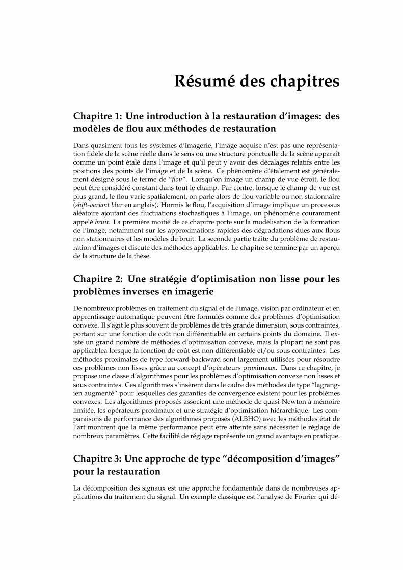
Chapitre 1: Une introduction à la restauration d’images: desmodèles de flou aux méthodes de restauration
Dans quasiment tous les systèmes d’imagerie, l’image acquise n’est pas une représenta-tion fidèle de la scène réelle dans le sens où une structure ponctuelle de la scène apparaîtcomme un point étalé dans l’image et qu’il peut y avoir des décalages relatifs entre lespositions des points de l’image et de la scène. Ce phénomène d’étalement est générale-ment désigné sous le terme de “flou”. Lorsqu’on image un champ de vue étroit, le floupeut être considéré constant dans tout le champ. Par contre, lorsque le champ de vue estplus grand, le flou varie spatialement, on parle alors de flou variable ou non stationnaire(shift-variant blur en anglais). Hormis le flou, l’acquisition d’image implique un processusaléatoire ajoutant des fluctuations stochastiques à l’image, un phénomène courammentappelé bruit. La première moitié de ce chapitre porte sur la modélisation de la formationde l’image, notamment sur les approximations rapides des dégradations dues aux flousnon stationnaires et les modèles de bruit. La seconde partie traite du problème de restau-ration d’images et discute des méthodes applicables. Le chapitre se termine par un aperçude la structure de la thèse.
Chapitre 2: Une stratégie d’optimisation non lisse pour lesproblèmes inverses en imagerie
De nombreux problèmes en traitement du signal et de l’image, vision par ordinateur et enapprentissage automatique peuvent être formulés comme des problèmes d’optimisationconvexe. Il s’agit le plus souvent de problèmes de très grande dimension, sous contraintes,portant sur une fonction de coût non différentiable en certains points du domaine. Il ex-iste un grand nombre de méthodes d’optimisation convexe, mais la plupart ne sont pasapplicablea lorsque la fonction de coût est non différentiable et/ou sous contraintes. Lesméthodes proximales de type forward-backward sont largement utilisées pour résoudreces problèmes non lisses grâce au concept d’opérateurs proximaux. Dans ce chapitre, jepropose une classe d’algorithmes pour les problèmes d’optimisation convexe non lisses etsous contraintes. Ces algorithmes s’insèrent dans le cadre des méthodes de type “lagrang-ien augmenté” pour lesquelles des garanties de convergence existent pour les problèmesconvexes. Les algorithmes proposés associent une méthode de quasi-Newton à mémoirelimitée, les opérateurs proximaux et une stratégie d’optimisation hiérarchique. Les com-paraisons de performance des algorithmes proposés (ALBHO) avec les méthodes état del’art montrent que la même performance peut être atteinte sans nécessiter le réglage denombreux paramètres. Cette facilité de réglage représente un grand avantage en pratique.
Chapitre 3: Une approche de type “décomposition d’images”pour la restauration
La décomposition des signaux est une approche fondamentale dans de nombreuses ap-plications du traitement du signal. Un exemple classique est l’analyse de Fourier qui dé-
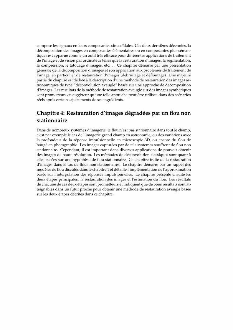
compose les signaux en leurs composantes sinusoïdales. Ces deux dernières décennies, ladécomposition des images en composantes élémentaires ou en composantes plus séman-tiques est apparue comme un outil très efficace pour différentes applications de traitementde l’image et de vision par ordinateur telles que la restauration d’images, la segmentation,la compression, le tatouage d’images, etc. . . . Ce chapitre démarre par une présentationgénérale de la décomposition d’images et son application aux problèmes de traitement del’image, en particulier de restauration d’images (débruitage et défloutage). Une majeurepartie du chapitre est dédiée à la description d’une méthode de restauration des images as-tronomiques de type “déconvolution aveugle” basée sur une approche de décompositiond’images. Les résultats de la méthode de restauration aveugle sur des images synthétiquessont prometteurs et suggèrent qu’une telle approche peut être utilisée dans des scénariosréels après certains ajustements de ses ingrédients.
Chapitre 4: Restauration d’images dégradées par un flou nonstationnaire
Dans de nombreux systèmes d’imagerie, le flou n’est pas stationnaire dans tout le champ,c’est par exemple le cas de l’imagerie grand champ en astronomie, ou des variations avecla profondeur de la réponse impulsionnelle en microscopie 3D, ou encore du flou debougé en photographie. Les images capturées par de tels systèmes souffrent de flou nonstationnaire. Cependant, il est important dans diverses applications de pouvoir obtenirdes images de haute résolution. Les méthodes de déconvolution classiques sont quant àelles basées sur une hypothèse de flou stationnaire. Ce chapitre traite de la restaurationd’images dans le cas de flous non stationnaires. Le chapitre démarre par un rappel desmodèles de flou discutés dans le chapitre 1 et détaille l’implémentation de l’approximationbasée sur l’interpolation des réponses impulsionnelles. Le chapitre présente ensuite lesdeux étapes principales: la restauration des images et l’estimation du flou. Les résultatsde chacune de ces deux étapes sont prometteurs et indiquent que de bons résultats sont at-teignables dans un futur proche pour obtenir une méthode de restauration aveugle baséesur les deux étapes décrites dans ce chapitre.
Symbols, Notations and SomeDefinitions
I briefly introduce here some of the notations, and definitions frequently used in thisthesis. Moreover, each chapter will recall the notations whenever they occur, and somenotations will be used in only some specific chapters, in this case they will be defined inthe context.
Throughout the manuscript, we denote a scalar by lower case Latin or Greek letter,a column vector by a bold lowercase letter, and a matrix by bold uppercase alphabet.In many places the two-dimensional images are represented by a column vector bylexicographical ordering of their pixels, until stated otherwise.
For x ∈ Rn, n denotes the length of the vector, xi ∈ R denotes the ith componentof x, and xT denotes the transpose of x.
For v ∈ Rn×2, vi ∈ R2 denotes the ith row vector of v, i.e., vi = (vi,1,vi,2).
For x,y ∈ Rn, 〈x,y〉Rn = xTy denotes the inner product on Rn.
For x ∈ Rn, ‖x‖2 =√xTx denotes the `2-norm on Rn.
For W ∈ Rn×n be a positive semidefinite matrix, ‖x‖W =√xTWx denotes the
weighted `2-norm on Rn associated withW .
For x ∈ Rn, ‖x‖∞ = maxi∈1,2,··· ,n|xi| denotes the `∞-norm on Rn.
The ·+ denotes the componentwise positive part of the input vector, i.e.,t+ = maxt,0, and and ·
· denote componentwise multiplication and divi-sion, respectively.
Let A be a linear transform A : Rn → Rn, and AT denotes its transpose.
In certain chapters dealing with iterative methods for optimization, f (k), ∇f (k), and∇2f (k) denote the function value, its gradient, and its Hessian, respectively, at iteration kfor some point x(k).

CHAPTER 1
An Introduction to ImageRestoration: From Blur Models to
Restoration Methods
You cannot depend on your eyes when your imagination is out of focus.– Mark Twain
Contents1.1 Introduction . . . . . . . . . . . . . . . . . . . . . . . . . . . . . . . . . . . . . . 41.2 A Brief Introduction to Imaging Systems . . . . . . . . . . . . . . . . . . . . . . 51.3 Modeling the Blur Degradation and its Approximations . . . . . . . . . . . . . 8
1.3.1 Shift-Invariant Blur . . . . . . . . . . . . . . . . . . . . . . . . . . . . . 101.3.2 Shift-Variant Blur . . . . . . . . . . . . . . . . . . . . . . . . . . . . . . 11
1.4 Noise in the Image Acquisition Process . . . . . . . . . . . . . . . . . . . . . . 181.5 Image Restoration . . . . . . . . . . . . . . . . . . . . . . . . . . . . . . . . . . 181.6 Bayesian Inference Framework for Image Restoration . . . . . . . . . . . . . . 20
1.6.1 Image Restoration Strategies . . . . . . . . . . . . . . . . . . . . . . . . 211.7 Observation Models . . . . . . . . . . . . . . . . . . . . . . . . . . . . . . . . . 231.8 Image and PSF Prior Models . . . . . . . . . . . . . . . . . . . . . . . . . . . . 25
1.8.1 Role of Hyperparameters and their Estimation . . . . . . . . . . . . . 271.9 Our Approach to Blind Image Deblurring . . . . . . . . . . . . . . . . . . . . . 271.10 Outline of the Thesis and Contributions . . . . . . . . . . . . . . . . . . . . . . 28
4Chapter 1. An Introduction to Image Restoration: From Blur Models to Restoration
Methods
Abstract
In almost every imaging system/situation, the captured image is not a faithful representa-tion of the actual scene, in the sense that a point-like structure in a scene does not appearas a point in the image. Furthermore, there can be also some relative shifts in the spatialpositions of the points in the image compared to their positions in the scene. This effectis commonly referred as blur. For narrow field-of-view imaging, the blur can be consid-ered constant throughout the field, while this is no longer the case for wide field-of-viewimaging, the blur varies over the field, yielding an effect called shift-variant blur. Apartfrom the blur, the image acquisition mechanism involves a statistical process, which addsfurther random fluctuations to the image, commonly called noise. The first half part ofthis chapter provides a detailed discussion on image formation model including the fastand sufficiently accurate shift-variant blur degradation models, and the different typesof noise with their statistical descriptions. The second half of the chapter introduces theimage restoration problem, and discusses the possible approaches for image restorationtechniques with their advantages and shortcomings. The chapter ends with an outline ofthis thesis work.
1.1 Introduction
Images play very important roles in many aspects of our life; from commercial photog-raphy to astronomy. The quality of images does matter in every field of application, inparticular, high resolution imaging is essential in many scientific applications. The qual-ity/resolution of images is not limited only by technological limitations in imaging sys-tems, but also due to the inherent properties of light and matter. With the advances intechnologies and fast computational methods, the quality/resolution of images have im-proved drastically in the last few decades. However, there still exists a good perspectivein improvement of imaging systems, pushing further the quality/resolution of images be-yond the physical limitations. There are many situations where, due to some physicalconstraints, higher quality/resolution image cannot be obtained without the help of nu-merical methods, such as image restoration techniques. A general objective of my thesisis to contribute this goal. To be more specific, the objective of my thesis is to improve theresolution of the images which have been degraded due to blur and noise by developingimage restoration techniques. The literature of imaging is full of many image restorationmethods, however a huge number of them are dedicated to restoration of images degradedonly by shift-invariant blur, which is still considered as a difficult problem in many cases.The emergence of restoration methods accounting for the blur variation across the field ofview (shift-variant blur) is recent. Image restoration accounting for shift-variant blur is arelatively more difficult task than shift-invariant blur, but essential for many applications.In wide field-of-view imaging, the blur varies due to several reasons, e.g., the optics (aber-rations), atmospheric turbulences for ground-based astronomical imaging, and relativemotion between the objects and the imaging system.
A more challenging and realistic situation in imaging is when the blur in an image isnot known beforehand. The image restoration technique in such situations is called blindimage restoration, since one needs to identify both the underlying blur and the crisp imagejust from the observed blurry and noisy image. To be more precise, the long-term objectiveof my thesis is to develop blind image restoration techniques for shift-variant blur. Sinceastronomical images captured by ground-based imaging system suffer from shift-variantblur, one of the goals of my thesis is also to develop methods that could restore those

1.2. A Brief Introduction to Imaging Systems 5
images, and this is why this work is a collaboration between the image formation andreconstruction group at the Laboratoire Hubert Curien CNRS UMR 5516 at Saint-Etienne,and the Centre de Recherche Astrophysique de Lyon CNRS UMR 5574 at Observatoirede Lyon. Blind image restoration technique, even in the case of shift-invariant blur, is adifficult problem for many imaging situations, thus it is still an active research topic withmany open questions. With shift-variant blur, it even becomes harder.
As is the case for many other PhD, I started my thesis with an effort to understandthe basics of the problem and to evaluate what has been already done in that direction.In order to be acquainted to the domain and to have more confidence, I started workingwith what has been already done, and progressively got into the difficulties of the prob-lems. Image restoration techniques boil down to numerical optimization problems, thusa significant part of my thesis is dedicated to development optimization algorithms suit-able for it. Once I became confident enough in solving optimization problems related toimage restoration, I dwelved into blind restoration of images with shift-invariant blur. Asignificant effort in my thesis has been put on blind image restoration techniques for im-proving the quality of astronomical images. I propose a blind image restoration techniquebased on image decomposition approach. The preliminary results on restoration of syn-thetic astronomical scenes are promising giving a hope for further improvements so thatit will be applicable to astronomical applications. Since in many imaging situations, in-cluding astronomical imaging, the degradations are due to the shift-variant blur, thus, Istarted working on image restoration with shift-variant blur. As said before, this is themost difficult problem in image restoration, and not much research has been publishedin this direction. In this regard, I have worked with an existing implementation of a shift-variant blur operator developed by my supervisors. At present, while I am completing mythesis, I have implemented a semi-blind image restoration technique for shift-variant blur,and have validated it on images with shift-variant blur due to optical aberrations. In whatfollows here, I explain the details of my PhD thesis work along with required theoreticaland experimental justifications/descriptions into chapters.
1.2 A Brief Introduction to Imaging Systems
Imaging systems are not able to capture a faithful representation of the actual scene. Inorder to give a sense of “faithful representation”, I start the chapter with a definition ofan imaging system. Mathematically, an imaging system (traditionally also referred to asa camera) is a mapping function, which maps a three dimensional object space into a twodimensional image space.
An Ideal Imaging System: An ideal camera is a concept in which the mapping is strictly aperspective projection. This implies that a point source in object space should appear as apoint on the image plane.
A Real Imaging System: In practice, a real camera does not involve just a simple perspec-tive projection but also other mapping functions, which appear for several reasons. Areal camera consists of several components: the media between the object and the imagesensors (including the atmosphere, and the lens), the finite size aperture, and the sensor.All these components add their contribution to the global degradation. The final effect ofthese extra mappings is that a point source in the scene does not appear as a point, butit can be spread over a large area (e.g., diffraction patterns are unbounded) in the imageplane, which is commonly known as blur. Moreover, the relative positions between the
6Chapter 1. An Introduction to Image Restoration: From Blur Models to Restoration
Methods
objectplane
Lens intercepts anangular sector ofradiated spherical
wave
Point spread functionin image plane
imageplane
Complete spherical waveradiated by point source
Partial spherical wave convergingto point spread functionvs.
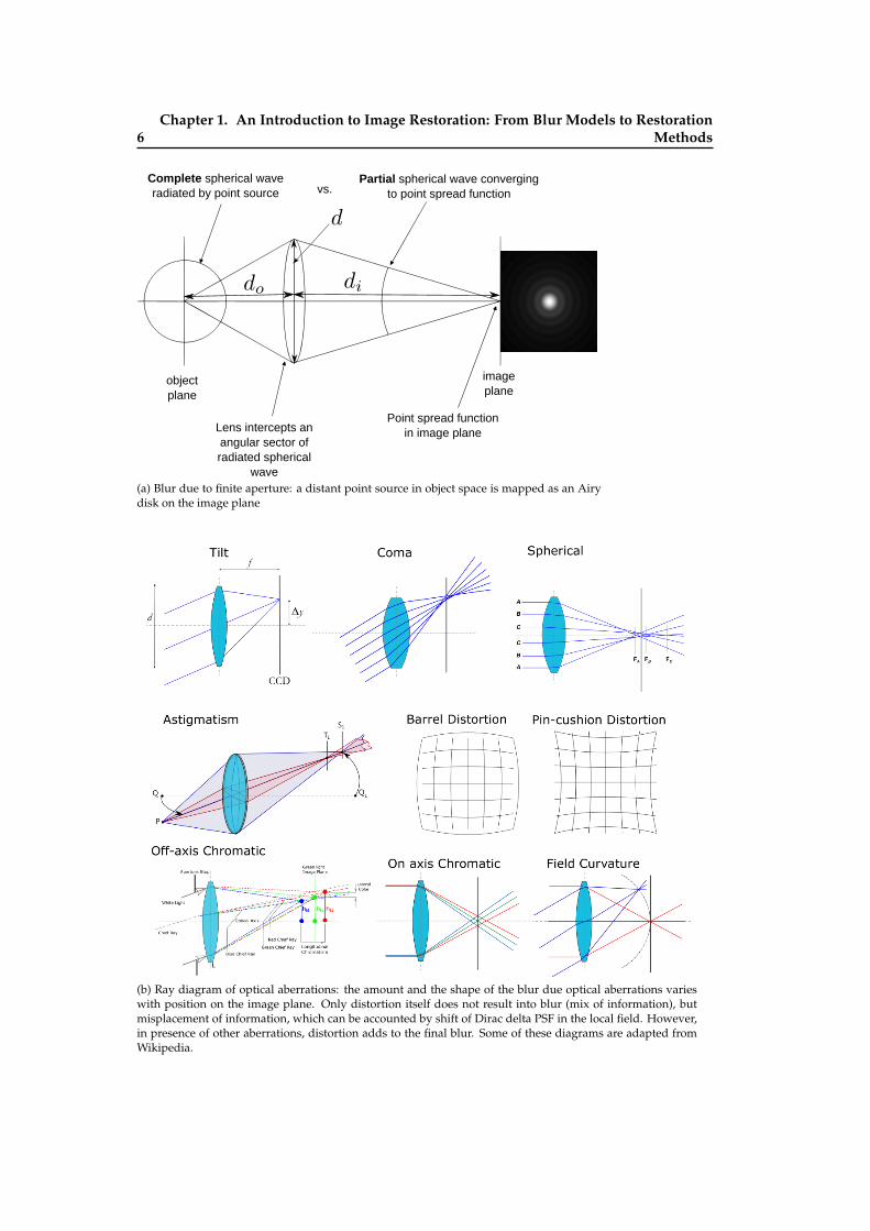
(a) Blur due to finite aperture: a distant point source in object space is mapped as an Airydisk on the image plane
(b) Ray diagram of optical aberrations: the amount and the shape of the blur due optical aberrations varieswith position on the image plane. Only distortion itself does not result into blur (mix of information), butmisplacement of information, which can be accounted by shift of Dirac delta PSF in the local field. However,in presence of other aberrations, distortion adds to the final blur. Some of these diagrams are adapted fromWikipedia.
1.2. A Brief Introduction to Imaging Systems 7
point sources in the scene are also altered in the image, a phenomenon commonly knownas geometrical distortion. Blur can be interpreted as a mixing of object information overthe image plane, whereas geometrical distortions can be interpreted as a spatial shift ofinformation.
Point Spread Function: The Point Spread Function (PSF) describes the response of animaging system to a point source in object space, and is a common quantitative measureof the blur introduced by a camera in the image, and it is also central to the modeling ofblur.
Three Fundamental Causes of Blur
Blur in an image can be due to several reasons, but most of them can be categorized intothe following three fundamental causes:
1. Blur due to the media between the object and the image plane: Commonly, terrestrial imag-ing systems and ground-based astronomical imaging systems involve two media be-tween the object and the image plane: the atmosphere and the lens system. In case ofground-based astronomical imaging, both the atmospheric turbulence and the lenssystem are accountable for irregular bending of light rays (or equivalently for thedeformation of the wavefronts) coming from distant objects. In the case of terrestrialimaging, the lens system is mostly responsible, and the effect is commonly referredto as optical aberrations: a departure of the performance of an optical system fromthe predictions of paraxial optics, as illustrated in Fig.1.1b. However, in long dis-tance terrestrial imaging the atmospheric turbulence is also involved. The irregularbending of light (or wavefront deformations) introduces blur in the image, and thefinal shape and the size of the PSF is dependent upon the wavelength of the light,and other several factors associated with the two media. In a narrow field-of-view,the PSF due to the media can be assumed to be constant over the entire image plane,but for a wide field-of-view, the PSF varies throughout the image plane, resultinginto shift-variant blur.
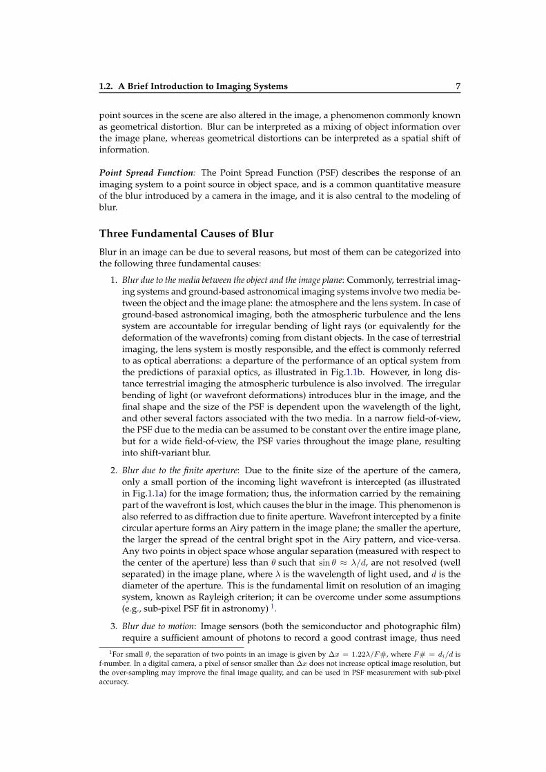
2. Blur due to the finite aperture: Due to the finite size of the aperture of the camera,only a small portion of the incoming light wavefront is intercepted (as illustratedin Fig.1.1a) for the image formation; thus, the information carried by the remainingpart of the wavefront is lost, which causes the blur in the image. This phenomenon isalso referred to as diffraction due to finite aperture. Wavefront intercepted by a finitecircular aperture forms an Airy pattern in the image plane; the smaller the aperture,the larger the spread of the central bright spot in the Airy pattern, and vice-versa.Any two points in object space whose angular separation (measured with respect tothe center of the aperture) less than θ such that sin θ ≈ λ/d, are not resolved (wellseparated) in the image plane, where λ is the wavelength of light used, and d is thediameter of the aperture. This is the fundamental limit on resolution of an imagingsystem, known as Rayleigh criterion; it can be overcome under some assumptions(e.g., sub-pixel PSF fit in astronomy) 1.
3. Blur due to motion: Image sensors (both the semiconductor and photographic film)require a sufficient amount of photons to record a good contrast image, thus need
1For small θ, the separation of two points in an image is given by ∆x = 1.22λ/F#, where F# = di/d isf-number. In a digital camera, a pixel of sensor smaller than ∆x does not increase optical image resolution, butthe over-sampling may improve the final image quality, and can be used in PSF measurement with sub-pixelaccuracy.
8Chapter 1. An Introduction to Image Restoration: From Blur Models to Restoration
Methods
a certain integration time, commonly referred to as the exposure time. Any relativemovement between the objects and the camera during the exposure time introducesan additional blur in the image, which is commonly called as motion blur. Besides,this motion blur, a certain amount of blur is inherent to semiconductor sensors, andthe mechanism involved in it, e.g., a small amount of photo electrons leakage be-tween the neighboring pixels, and due to integration over the photosensitive area ofthe pixels.
In general, the blur due to finite aperture (except in diffraction limited imaging case) andsemiconductor image capturing mechanism is significantly smaller than the blur intro-duced by the propagating media, optical aberration and relative motion.
1.3 Modeling the Blur Degradation and its Approximations
Remark: This section is adapted from our journal paper “Fast Approximation of Shift-Variant Blur”[Denis 2015].
As mentioned in the definition, the point-spread-function (PSF) fully characterizes the blurintroduced in an image. In image deblurring applications, it is necessary to simulate theeffect of the blur introduced by the camera system on the image of the object. Thus, oneneeds an image blurring model, and a fast numerical implementation of it. A fairly generalmodeling of blurring in the continuous domain takes the form of a Fredholm integralequation of the first kind:
y(r) =
∫h(r, s) x(s)ds (1.1)
where x denotes ideal perspective projected (crisp) image, h(·, s) denotes the PSF at loca-tion s, and y denotes the blurry image. The PSF h may be considered as the conditionalprobability density p(r|s) describing the probability that a photon entering the system atlocation s lands at location r in the image plane. Here, the locations r and s are vectorsdefining the 2D or 3D coordinates, a d-dimensional vector in the following. In some cases,the PSF is shift-invariant ∀t, h(r, s) = h(r+ t, s+ t), i.e., it depends only on the differencer−s. In this case, the blurring model (1.1) becomes a convolution and the system is calledisoplanatic. In many cases, the PSFs vary smoothly with the input location s. In order todistinguish true PSF variations from simple shifts of the PSF h(r, s) due to changes in theinput location s, it will prove useful in the following to consider un-shifted PSF definedby: k(r, s) = h(r − s, s). The above blurring model (1.1) can then be rewritten under theform:
y(r) =
∫k(r − s, s) x(s)ds (1.2)
In the general case, evaluation of the blurring model (1.1) is computationally intensive.As explained in [Gilad 2006], this evaluation becomes computational less expensive if aseparable bilinear approximation of the kernel is used:
k(r, s) ≈∑p
mp(r) wp(s) (1.3)
where k(r, s) = h(r + s, s) is the centered PSF, mp are components of the PSF modeland wp are the weights depending on the location s, which should follow the condition∑p wp(s) = 1 2. The trade off between accuracy of equivalent PSF and computational
2This condition ensures that if mp, the components of the PSF model, are normalized, i.e.,∑
smp(s) = 1,then each of the interpolated PSFs k(r, s) are also normalized.
1.3. Modeling the Blur Degradation and its Approximations 9
expense can be easily controlled by varying the density of the sampling of PSFs in thefield of view. With constant weights wp(s) = wp, the corresponding kernel would beshift-invariant. By letting the weight wp(s) of each model mp vary with the location s, ashift-variant model is derived. With this approximation, the blurring model (1.1) can bereduced to a simple sum of convolutions:
y(r) ≈[∑
p
mp ∗ (wp x)
](r) (1.4)
where ∗ is the classical notation for convolution, and is for componentwise multiplica-tion. Equation (1.4) approximates the shift-variant operator as a sum of convolutions ofweighted versions of the input image x. Existence of fast algorithms for discrete convolu-tion makes this decomposition very useful, as we will see in the following.
Discretization of the above blurring operation is necessary from an implementationpoint of view. An approximation of the discrete version of the blurring operation can alsobe considered from the point of view of matrix decomposition/approximation problems.Discretization of the above blurring model (1.1) can be written as a matrix-vector product:
y = H x = X h (1.5)
where y ∈ Rn is the n-pixels blurry image, x ∈ Rm is the m-pixels crisp image, and H ∈Rn×m is the blurring operator. These discrete images are represented as column vectors bylexicographically ordering their pixel values. The matrixH defining the discrete operatoris obtained by sampling the continuous operator h at locations (ri)i=1,··· ,n and (si)i=1,··· ,m:
∀i : 1 ≤ i ≤ n; ∀j : 1 ≤ j ≤ mHi,j = h(ri, sj)∆j (1.6)
where ∆j is the elementary volume measure ensuring normalization of H and possiblenonuniform sampling of the input field (sj)j=1,··· ,m. The jth column H ·,j correspondsto the sampled PSF for a point-source located at sj . By analogy, X ∈ Rn×m is the cor-responding discrete blurring operator obtained by sampling the continuous image x. Inthe coming paragraphs, all the discussions will be based only on the operator H , but areanalogously applicable to operatorX .
Discretization (1.6) has some limitations. Using the generalized sampling theory, asdescribed by in [Chacko 2013], Denis et al. in [Denis 2015] write the blurring operation ina more generalized form as:
yi ≈∫ϑpixi (r)
∫h(r, s)
∑j
ϑintj (s) xj ds dr (1.7)
In this generalization, a continuous image xint is defined by using a sequence of discretecoefficients xj as the weights of a set of basis function:
xint(s) =∑j
ϑintj (s) xj ,
with ϑintj a shifted copy of a certain “mother” basis function ϑint (e.g., B-splines). Coeffi-cients xj are typically chosen as to minimize the approximation error, i.e., the continuousimage xint corresponds to the orthogonal projection of x onto the subspace spanned by

10Chapter 1. An Introduction to Image Restoration: From Blur Models to Restoration
Methods
basis function ϑintj . Digitization of the blurred image by the sensor involves integration onthe sensitive area of the pixel that is modeled as:
yi =
∫ϑpixi (r) g(r) dr,
with ϑpixi a shifted copy of the pixel spatial sensitivity (e.g. indicator function of the sensi-tive area).
Using the above generalization of the blurring operation, the discrete operator H canbe defined as:
∀i : 1 ≤ i ≤ n; ∀j : 1 ≤ j ≤ m
Hi,j =
∫∫ϑpixi (r) h(r, s) ϑintj (s) ds dr (1.8)
By using the separable approximation as in (1.3), the collectionK of the centered PSFs, asintroduced in the continuous case, is written as:
K ≈∑p
mp(i) wp(j) ↔ K ≈∑p
mp wTp (1.9)
and the shift-variant blurring operator as the sum of convolutions with prior weightings:
H ≈∑p
conv(mp) diag(wp) (1.10)
where conv(mp) denotes the discrete convolution matrix with kernel mp, diag(wp) is adiagonal matrix whose diagonal is given by the vector wp.
1.3.1 Shift-Invariant Blur
For a small field-of-view, the blur introduced by any of the causes mentioned in Section1.2 can be considered to be shift-invariant. For shift-invariant PSF, K is a rank-one ma-trix with identical columns equal to the single PSF k. The operator H , in this case cor-responds to a discrete convolution. While discrete circular convolution is mapped as asimple componentwise product in Fourier domain, the discrete convolution needs ade-quate zero-padding and cropping operations, and thus the blur operator can be writtenas:
H ≡ conv(k) = R F−1 diag(k) F︸ ︷︷ ︸circular convolution
Ex
and (1.11)
X ≡ conv(x) = R F−1 diag(x) F︸ ︷︷ ︸circular convolution
Eh
where Eh and Ex are expansion operators that add zeros to the boundaries of the inputsignals: the image and the PSF, respectively, R is a restriction operator that truncates theoutput blurred signal to the original size of the input signal, F and F−1 are the direct andinverse discrete Fourier transforms, and k is the discrete Fourier transform of the PSF:
k = F Eh k
and (1.12)
x = F Ex x
1.3. Modeling the Blur Degradation and its Approximations 11
Now, the application of the blur operator H to an image x can be computed very effi-ciently using fast Fourier transforms (FFT), and because of the zero-padding followed bychopping operations, the blurring operation is no more circular convolution.
1.3.2 Shift-Variant Blur
Most of the fast shift-variant blurring operators in the literature are based on the separablelinear approximation (1.3) or are similar to it. However, recently [Escande 2014] has pro-posed an approach based on the wavelet transform to efficiently encode the shift-variantblur operator. Now, in the following, we will see some of the relevant approximations.
Piecewise Constant PSFs:The simplest and fastest known shift-variant approximations is the piecewise constant PSFsapproximation. In this approximation, an image is partitioned into P small-enough re-gions so that the PSF within each region can be considered invariant, and then each regionis treated with shift-invariant blur operator. The collection K of the centered PSF is arank-P matrix. Using the linear separable approximation (1.10), the piecewise constant bluroperator can be written as:
H =
P∑p=1
conv(kp) diag(ιp) (1.13)
where ιp is the vector of binary weights indicating the locations sj belonging to the pthregion of the input field. Being the fastest approximation, this approach has adverseconsequences; it generates important artifacts at the region’s boundaries due to thediscontinuities in the PSFs approximation.
Smoothly Varying PSFs and their Local Approximation:To tackle artifacts at the region boundaries, smoothly varying PSFs approximations areproposed in the literature. In many applications, in fact, the PSFs vary smoothly acrossthe field. In such cases, a PSF (e.g., column kj from K) can be well approximated by theother neighboring PSFs. If P columns of K are selected, i.e., kp | p ∈ GP , where GPrepresents the set of all points on a given grid, each column ofK can be approximated bythe weighted sum of P columns out of M (typically with P M ):
K ≈∑p∈GP
kp ϕTp (1.14)
The interpolation weightsϕTp are no longer constrained to take binary values, and weightsare spatially localized: they are nonzero only on a spatial neighborhood surrounding lo-cation s. The extend of that neighborhood depends on the interpolation order, e.g., itcorresponds to a square twice the grid step along each dimension for first-order (linear)interpolation. Using the approximation (1.14), the blur operator in (1.10) becomes:
H ≈∑p∈GP
conv(kp) diag(ϕp) (1.15)
The weights localizations make this decomposition very suitable from a computationalpoint of view: full-field convolution computations are not necessary since the precedingweighting operation introduces zeros everywhere except on regions with size twice thegrid step. This formulation of a shift-variant blur operator has been independently sug-gested in [Gilad 2006] and [Hirsch 2010]. Denis et al. in [Denis 2011] show that this for-
12Chapter 1. An Introduction to Image Restoration: From Blur Models to Restoration
Methods
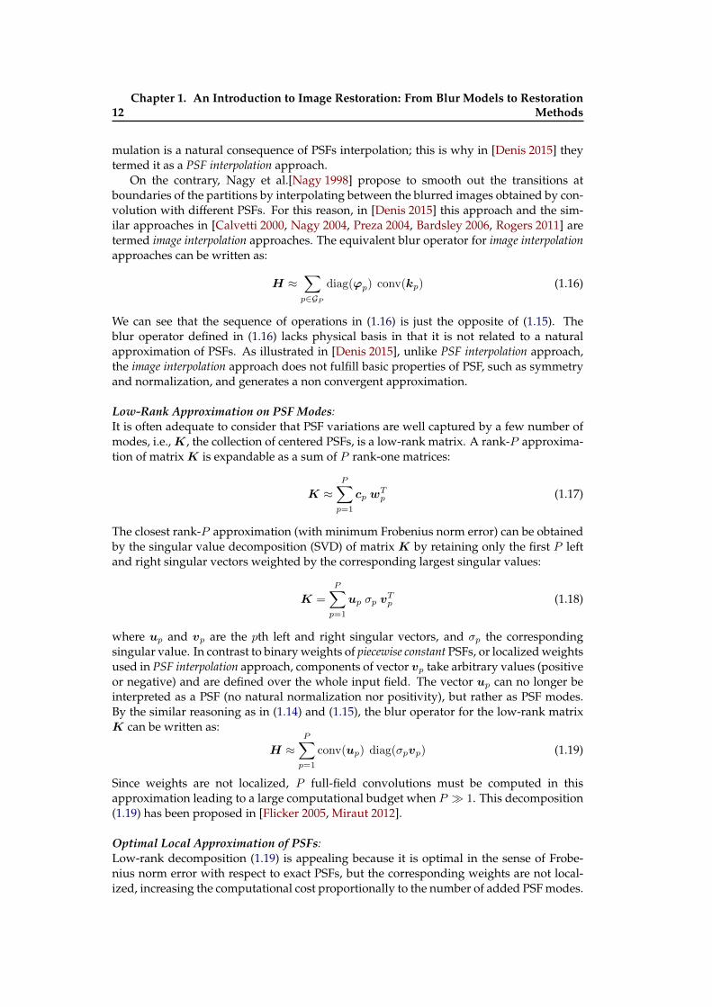
mulation is a natural consequence of PSFs interpolation; this is why in [Denis 2015] theytermed it as a PSF interpolation approach.
On the contrary, Nagy et al.[Nagy 1998] propose to smooth out the transitions atboundaries of the partitions by interpolating between the blurred images obtained by con-volution with different PSFs. For this reason, in [Denis 2015] this approach and the sim-ilar approaches in [Calvetti 2000, Nagy 2004, Preza 2004, Bardsley 2006, Rogers 2011] aretermed image interpolation approaches. The equivalent blur operator for image interpolationapproaches can be written as:
H ≈∑p∈GP
diag(ϕp) conv(kp) (1.16)
We can see that the sequence of operations in (1.16) is just the opposite of (1.15). Theblur operator defined in (1.16) lacks physical basis in that it is not related to a naturalapproximation of PSFs. As illustrated in [Denis 2015], unlike PSF interpolation approach,the image interpolation approach does not fulfill basic properties of PSF, such as symmetryand normalization, and generates a non convergent approximation.
Low-Rank Approximation on PSF Modes:It is often adequate to consider that PSF variations are well captured by a few number ofmodes, i.e.,K, the collection of centered PSFs, is a low-rank matrix. A rank-P approxima-tion of matrixK is expandable as a sum of P rank-one matrices:
K ≈P∑p=1
cp wTp (1.17)
The closest rank-P approximation (with minimum Frobenius norm error) can be obtainedby the singular value decomposition (SVD) of matrix K by retaining only the first P leftand right singular vectors weighted by the corresponding largest singular values:
K =
P∑p=1
up σp vTp (1.18)
where up and vp are the pth left and right singular vectors, and σp the correspondingsingular value. In contrast to binary weights of piecewise constant PSFs, or localized weightsused in PSF interpolation approach, components of vector vp take arbitrary values (positiveor negative) and are defined over the whole input field. The vector up can no longer beinterpreted as a PSF (no natural normalization nor positivity), but rather as PSF modes.By the similar reasoning as in (1.14) and (1.15), the blur operator for the low-rank matrixK can be written as:
H ≈P∑p=1
conv(up) diag(σpvp) (1.19)
Since weights are not localized, P full-field convolutions must be computed in thisapproximation leading to a large computational budget when P 1. This decomposition(1.19) has been proposed in [Flicker 2005, Miraut 2012].
Optimal Local Approximation of PSFs:Low-rank decomposition (1.19) is appealing because it is optimal in the sense of Frobe-nius norm error with respect to exact PSFs, but the corresponding weights are not local-ized, increasing the computational cost proportionally to the number of added PSF modes.
1.3. Modeling the Blur Degradation and its Approximations 13
The PSF interpolation approach is preferable in this regard since weights localizations pre-vent the computation of full-field convolutions, saving computation costs especially forsmall PSF supports. Taking into account the advantages of these approaches, Denis et al.[Denis 2015] propose an intermediate solution where the weights are local, and the Frobe-nius norm error between the approximated PSFs and the exact PSFs is minimal. Theydefine the optimal local approximation of matrixK as:
K ≈P∑p=1
c∗p w∗pT (1.20)
where PSF c∗pPp=1 and weights w∗pPp=1 are optimal solutions of the following minimiza-tion problem:
c∗p,w∗p
Pp=1
= arg mincp,wpPp=1
‖K −P∑p=1
cp wTp ‖2F (1.21)
where the weight vectors wp are restricted to the support of interpolation weightsupp(ϕp):
∀p, supp(wp) ⊂ supp(ϕp) (1.22)
for a fixed PSF interpolation scheme ϕ1, · · · ,ϕp. The minimization problem (1.21) isbiconvex; a local optimum can be found by alternate convex search (see [Denis 2015] forthe detail of the minimization algorithm). With the so-found optimal PSFs and weights,the shift-variant blur operator H is approximated, following the decomposition in (1.19),as:
H ≈P∑p=1
conv(c∗p) diag(w∗p) (1.23)
Optimal vectors c∗p and optimal weights w∗p can be computed beforehand (i.e., for a givenmodelH). The complexity of approximation (1.23) is the same as approximation (1.19).
Comparison of Blur Approximations:In the literature of shift-variant blur approximations, much of the attention has been paidto the computational aspect, whereas the equivalent PSF is never mentioned explicitly.Yet, it is essential to relate a given approximation method to the corresponding approx-imation in terms of PSF. The authors in [Denis 2015] provide a detailed discussion onit, which is summarized here for the sake of comparison. The PSF kj for a point sourcelocated at sj is approximated by an equivalent PSF kj that depends upon the model:
With a shift-invariant PSF model (1.11) : k(Cst)j = k.
With a piecewise constant PSF model (1.13) : k(PCst)j = kp, for p such that ιp(j) = 1.
With a PSF interpolation based model (1.14) : k(PSFInterp)
j =∑p∈GP ϕp(j) kp, where ϕp(j)
are interpolation weights.
With an image interpolation based model (1.16) : k(ImageInterp)
j =∑p∈GP diag( ~ϕp
j) kp, where~ϕpj(i) is the interpolation weight at location ri + sj .
With a decomposition on modes based model (1.19) : k(Modes)j =
∑p σpvp(j) up.
Finally, with optimal local approximation based model (1.23) : k(OptLoc)j =
∑pw∗p(j) c
∗p.
Depending on the approximation method, the equivalent PSF can fulfill some desir-able properties of PSF, which are pointed out in Table 1.1. We can see that PSF interpolation
14Chapter 1. An Introduction to Image Restoration: From Blur Models to Restoration
Methods
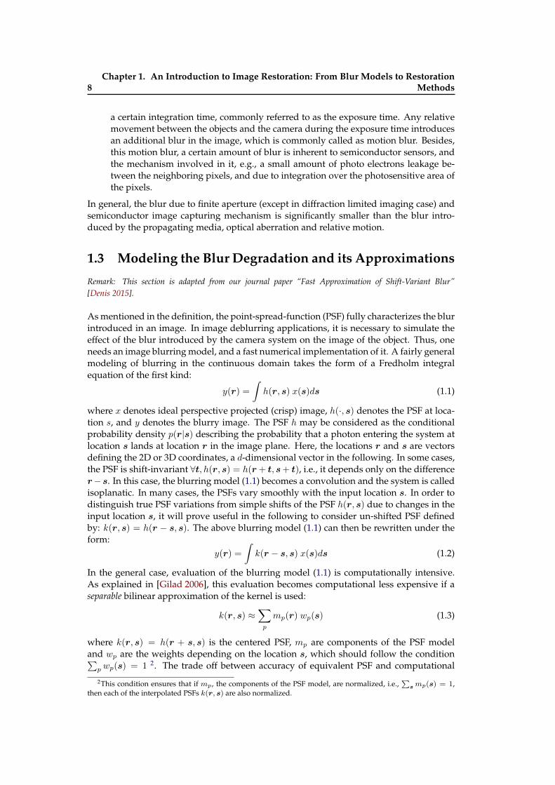
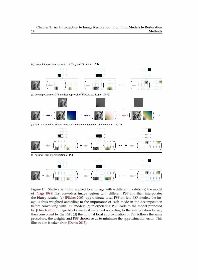
Figure 1.1: Shift-variant blur applied to an image with 4 different models: (a) the modelof [Nagy 1998] first convolves image regions with different PSF and then interpolatesthe blurry results; (b) [Flicker 2005] approximate local PSF on few PSF modes, the im-age is thus weighted according to the importance of each mode in the decompositionbefore convolving with PSF modes; (c) interpolating PSF leads to the model proposedby [Hirsch 2010], image blocks are first weighted according to the interpolation kernel,then convolved by the PSF; (d) the optimal local approximation of PSF follows the sameprocedure, the weights and PSF chosen so as to minimize the approximation error. Thisillustration is taken from [Denis 2015].
1.3. Modeling the Blur Degradation and its Approximations 15
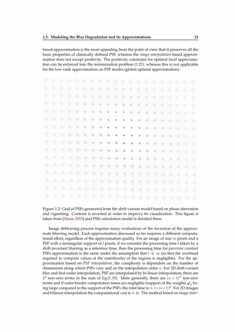
based approximation is the most appealing from the point of view that it preserves all thebasic properties of classically defined PSF, whereas the image interpolation based approxi-mation does not except positivity. The positivity constraint for optimal local approxima-tion can be enforced into the minimization problem (1.21), whereas this is not applicablefor the low-rank approximation on PSF modes (global optimal approximation).
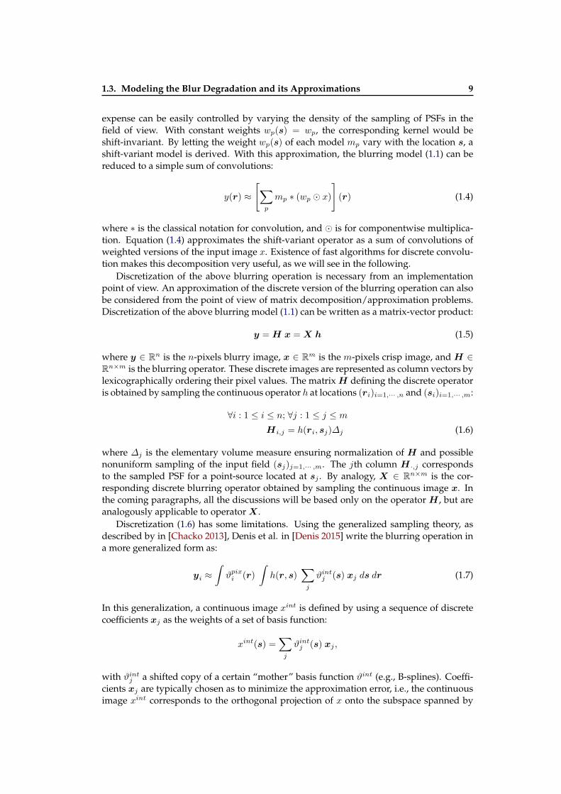
Figure 1.2: Grid of PSFs generated from the shift-variant model based on phase aberrationand vignetting. Contrast is inverted in order to improve its visualization. This figure istaken from [Denis 2015] and PSFs simulation model is detailed there.
Image deblurring process requires many evaluations of the inversion of the approxi-mate blurring model. Each approximation discussed so far requires a different computa-tional effort, regardless of the approximation quality. For an image of size m pixels and aPSF with a rectangular support of l pixels, if we consider the processing time t taken by ashift-invariant blurring as a reference time, then the processing time for piecewise constantPSFs approximation is the same under the assumption that l m (so that the overheadrequired to compute values at the outerborder of the regions is negligible). For the ap-proximation based on PSF interpolation, the complexity is dependent on the number ofdimensions along which PSFs vary and on the interpolation order o. For 2D shift-variantblur and first-order interpolation, PSF are interpolated by bi-linear interpolation; there are22 non-zero terms in the sum of Eq.(1.15). More generally, there are (o + 1)d non-zeroterms and if outer-border computation times are negligible (support of the weights ϕp be-ing large compared to the support of the PSF), the total time is≈ t×(o+1)d. For 2D imagesand bilinear interpolation the computational cost is≈ 4t. The method based on image inter-
16Chapter 1. An Introduction to Image Restoration: From Blur Models to Restoration
Methods
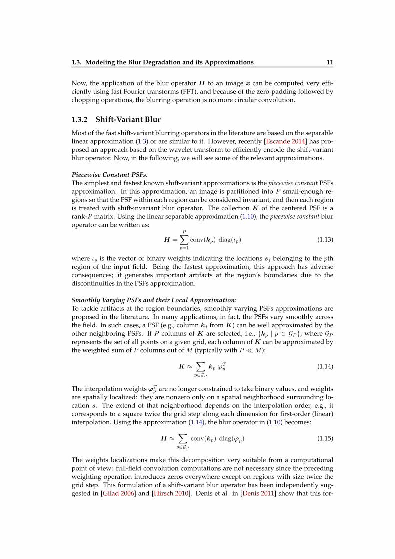
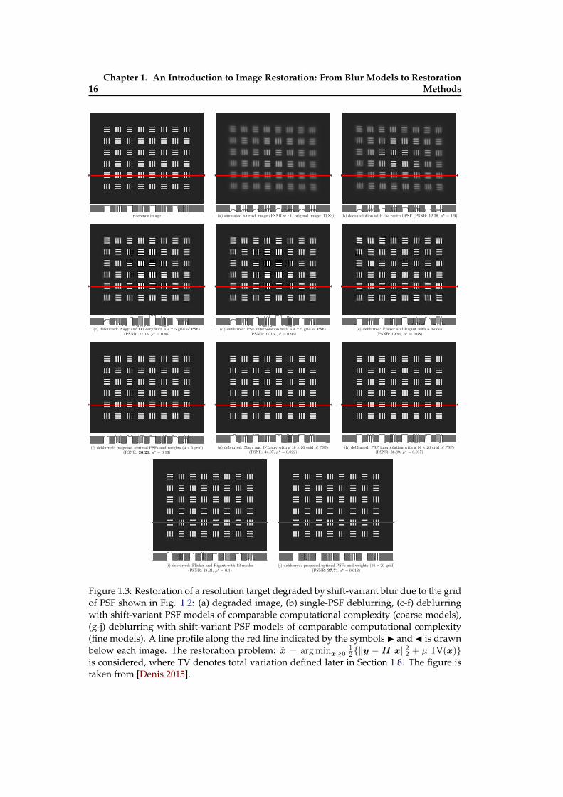
Figure 1.3: Restoration of a resolution target degraded by shift-variant blur due to the gridof PSF shown in Fig. 1.2: (a) degraded image, (b) single-PSF deblurring, (c-f) deblurringwith shift-variant PSF models of comparable computational complexity (coarse models),(g-j) deblurring with shift-variant PSF models of comparable computational complexity(fine models). A line profile along the red line indicated by the symbols I and J is drawnbelow each image. The restoration problem: x = arg minx≥0
12‖y −H x‖22 + µ TV(x)
is considered, where TV denotes total variation defined later in Section 1.8. The figure istaken from [Denis 2015].
1.3. Modeling the Blur Degradation and its Approximations 17
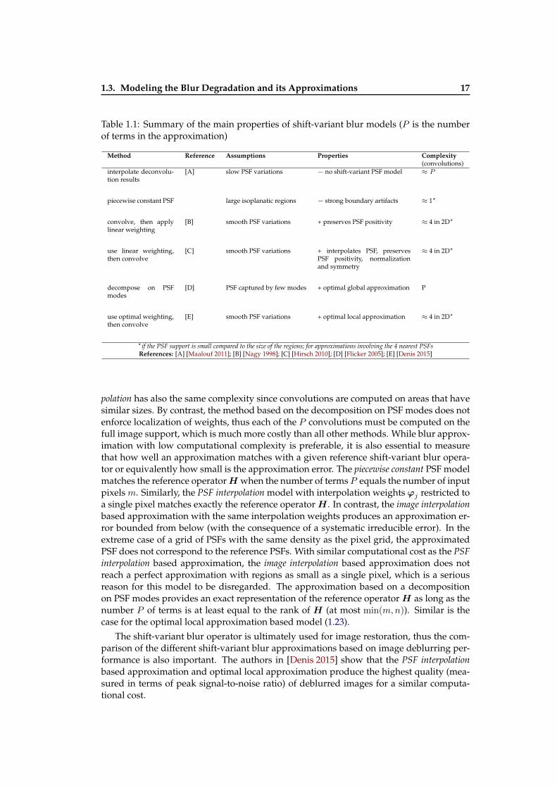
Table 1.1: Summary of the main properties of shift-variant blur models (P is the numberof terms in the approximation)
Method Reference Assumptions Properties Complexity(convolutions)
interpolate deconvolu-tion results
[A] slow PSF variations − no shift-variant PSF model ≈ P
piecewise constant PSF large isoplanatic regions − strong boundary artifacts ≈ 1?
convolve, then applylinear weighting
[B] smooth PSF variations + preserves PSF positivity ≈ 4 in 2D?
use linear weighting,then convolve
[C] smooth PSF variations + interpolates PSF, preservesPSF positivity, normalizationand symmetry
≈ 4 in 2D?
decompose on PSFmodes
[D] PSF captured by few modes + optimal global approximation P
use optimal weighting,then convolve
[E] smooth PSF variations + optimal local approximation ≈ 4 in 2D?
?if the PSF support is small compared to the size of the regions; for approximations involving the 4 nearest PSFsReferences: [A] [Maalouf 2011]; [B] [Nagy 1998]; [C] [Hirsch 2010]; [D] [Flicker 2005]; [E] [Denis 2015]
polation has also the same complexity since convolutions are computed on areas that havesimilar sizes. By contrast, the method based on the decomposition on PSF modes does notenforce localization of weights, thus each of the P convolutions must be computed on thefull image support, which is much more costly than all other methods. While blur approx-imation with low computational complexity is preferable, it is also essential to measurethat how well an approximation matches with a given reference shift-variant blur opera-tor or equivalently how small is the approximation error. The piecewise constant PSF modelmatches the reference operatorH when the number of terms P equals the number of inputpixels m. Similarly, the PSF interpolation model with interpolation weights ϕj restricted toa single pixel matches exactly the reference operatorH . In contrast, the image interpolationbased approximation with the same interpolation weights produces an approximation er-ror bounded from below (with the consequence of a systematic irreducible error). In theextreme case of a grid of PSFs with the same density as the pixel grid, the approximatedPSF does not correspond to the reference PSFs. With similar computational cost as the PSFinterpolation based approximation, the image interpolation based approximation does notreach a perfect approximation with regions as small as a single pixel, which is a seriousreason for this model to be disregarded. The approximation based on a decompositionon PSF modes provides an exact representation of the reference operator H as long as thenumber P of terms is at least equal to the rank of H (at most min(m,n)). Similar is thecase for the optimal local approximation based model (1.23).
The shift-variant blur operator is ultimately used for image restoration, thus the com-parison of the different shift-variant blur approximations based on image deblurring per-formance is also important. The authors in [Denis 2015] show that the PSF interpolationbased approximation and optimal local approximation produce the highest quality (mea-sured in terms of peak signal-to-noise ratio) of deblurred images for a similar computa-tional cost.
18Chapter 1. An Introduction to Image Restoration: From Blur Models to Restoration
Methods
1.4 Noise in the Image Acquisition Process
In addition to the deformations introduced in the images due to blur, which can be deter-ministic in nature 3, the images suffer from further degradation due to a statistical processinvolved in the image capturing mechanism, whose effect is commonly known as noise.The two fundamental causes of noise in an image are: the particle nature of light, and theconstant thermal agitation of electrons in semiconductor sensor and amplifiers.
The light coming from the observed source is detected in the form of photons. Thephotons impinging the image sensor generate a proportional number of photoelectrons.The expected number of photons detected in a pixel is proportional to the brightness dis-tribution integrated on the pixel area during the exposure time. The number of photonsimpinging the sensor within the exposure time is modeled by a Poisson process, and theeffect of the uncertainty in the Poisson process is called Poisson or shot noise. Indepen-dently of this Poisson process of photoelectrons generation, there is always a constantthermal agitation of electrons in the semiconductor sensor and amplifier. The distributionof the thermally agitated electrons can be approximately modeled by a Gaussian process.This thermally agitated electrons adds to the photoelectrons, and the effect is called de-tector noise. Both of these noises happen to be independent of each other, and happenindependently at each pixel in the sensor. Thus, these noises are also referred to as whitenoise. The Poisson noise is significantly perceptible in the image captured under dim lightcondition when the number of photons is sufficiently small so that uncertainties due tothe Poisson process, which describes the occurrence of independent random events, are ofsignificance. The mean and variance is the same for a Poisson process, thus the varianceof Poisson noise is the number of photons arriving to the image sensor within a certainexposure time. The detector noise in an image is perceptible as a constant noise level indark areas whose mean is zero and the variance is directly related to the absolute temper-ature of the sensor and amplifier. A part of detector noise called “dark current” due to thethermal agitation of the electrons can be minimized by using a supercooled image sensor.
Except these two fundamental noise sources in image acquisition processes, there couldbe some other noise sources too, but most of them can be avoided or removed from theimages because either their nature is deterministic or their origins can be easily traced. Forexample all pixels in a sensor do not behave exactly the same, but their behavior follows apattern for a fixed sensor, so the final effect can be easily estimated by calibration methodsand removed from the image. Another example of noise is impulsive or salt-and peppernoise, which can be due to the error in analog-to-digital converter or bit error in transmis-sion, but this noise can be easily avoided by a certain care. Thus, in image restoration anddenoising literature the main concern is only on the two fundamental noises, the Poissonand the detector noise. This is why we limit our considerations to these two fundamentalnoises while discussing image restoration problems.
1.5 Image Restoration
As we saw in our previous discussion, the final raw image acquired from a camerasystem is not a simple perspective projection of the 3D world onto the image plane, butit is degraded: distorted and corrupted by blur and noise, respectively. It is inevitablefor many imaging systems and situations to introduce a certain level of distortion andcorruption. However, for several reasons, either for aesthetic purpose or for scientificmeasurement and analysis purpose, it is crucial to have fair representation of the objects
3blur due to atmospheric turbulence may not be deterministic.

1.5. Image Restoration 19
in images. Image restoration is a technique to recover the underlying original image giventhe blurry and noisy image. Image restoration can be used to suppress noise, improve theresolution, the contrast of blurred structures in images.
A Generic Image Formation Model: Before one can devise any image restoration (reverse)technique, one should have an accurate forward measurement/degradation model, re-ferred as image formation model, in this context. A generic image formation model, whichtakes into account the blur and the two noise processes, discussed previously, can be writ-ten as:
y = P(H x) + n (1.24)
where y ∈ Rn is the observed blurry and noisy image, P represents Poisson process withexpected value (H x), and n ∼ N (0, σ2) is an additive detector noise (it is assumed thatthe detector bias has been removed). Here again, H ∈ Rn×m denotes the discrete bluroperator, and x ∈ Rm represents the original unknown image.
In the following, with some abuse of notation, both a grid of PSFs in the case of theshift-variant blur and a single PSF in the case of shift-invariant blur will be representedby h, and the corresponding blurring operator byH .
Image Restoration Problem: Image restoration problem can be stated as inferring the trueunderlying image, x, given the observed blurry and noisy image, y. Two situations mayarise:
1. when the most significant part of the degradation comes from noise and blur is ne-glected, then image restoration is called image denoising,
2. when the significant part of the degradation is due to blur, and some noise also, thenthe resolution of the image can be improved by a restoration technique called imagedeblurring.
From a theoretical point of view, image denoising problems are comparatively easier thanimage deblurring problems, at least for the reasons discussed in the next paragraph.
Image deblurring problems can be further categorized into two classes:
1. In some imaging situations, the PSFs h are assumed to be known perfectly before-hand, either from simulations or obtained by calibration methods or derived analyt-ically from parametric models, then the image deblurring problem is referred to asnonblind image deblurring.
2. In many practical imaging situations, the PSFs are not known beforehand, either be-cause they cannot be calibrated at the moment when the image is being captured orpreviously calibrated PSFs are no more applicable (are far from the underlying truePSF), then both the underlying original image and PSF are assumed to be unknown,and the image deblurring is referred to as blind image deblurring.
Nonblind image deblurring is considerably much easier than blind image deblurring, atleast, for the following degeneracies associated with shift-invariant blind deblurring:
• scaling: ( 1τ h) ∗ (τ x) = h ∗ x
• shift: x ∗ h = (δ−s ∗ x) ∗ (δs ∗ h), where δs and δ−s is shifted Dirac-delta function.
• identity: δ ∗ y = y (no blur explanation case)
• reducibility: (g ∗ x) ∗ h = x ∗ (g ∗ h)
20Chapter 1. An Introduction to Image Restoration: From Blur Models to Restoration
Methods
• inversion: x ∗ h = (s ∗ x) ∗ (s−1 ∗ h)
In the upcoming sections, we will see how these degeneracies can be tackled in blindimage deblurring by taking into account certain physical constraints and justifiableassumptions.
Image deblurring, in general, belongs to the category of ill-posed inverse problems,which means that any attempt to estimate the unknown quantities, without taking into ac-count any information about the unknown quantities will always result into a failure; thesolution will be corrupted by an amplified noise. In other words, because of the blurringoperation, some high frequency information is permanently lost from the observed blurryand noisy image, thus it is impossible to recover back the underlying original image bysimple inversion of the blur operator( i.e., x = H−1y) without considering any furtherinformation on the underlying original image, even if the blurring operator is known per-fectly. This fact motivates/obliges us to recognize that the image deblurring problemsshould be tackled by the methods of statistical estimation theory or regularization princi-ples. The statistical estimation methods based on Bayesian inference are the most popularand successful methods for their flexibility to include all the subjective beliefs on the un-knowns, and the other related methods can be interpreted easily from a Bayesian point ofview. The methods based on the maximum likelihood estimation, the maximum entropy,regularizations, etc, can be seen as special cases of Bayesian inference, this is described inthe next section.
For blind image deblurring, the existing approaches can be categorized into twoclasses: a priori blur identification methods, and joint identification methods. In the for-mer approach, the blur is identified first from the given blurry and noisy image, then it isused with a nonblind image deblurring scheme to estimate the underlying original image.The majority of existing methods fall into the second class, where the image and the blurare identified simultaneously. In practice many methods in this class use an alternating ap-proach to estimate the unknown x and h rather than truly finding the joint solution. Mostof the methods in both classes fall into the Bayesian inference framework, however therealso exists other methods not belonging to this approach (for example see [Campisi 2007]).In this thesis, my works are mostly based on Bayesian inference framework.
1.6 Bayesian Inference Framework for Image Restoration
It is a common practice in the Bayesian inference framework to consider all parameters andobservable variables as unknown stochastic quantities, assigning probability distributionsbased on subjective beliefs. Thus, in image deblurring problem, the original underlyingimage x, the PSF h, and the noisen in image formation model (1.24) can be treated as sam-ples drawn from random fields, with corresponding prior probability density functions(PDFs) that model our knowledge about the imaging process, the nature of images andthe PSF. Further, these distributions depend on some parameters which will be denotedby Θ. The parameters of the prior distributions are commonly referred as hyperparameters.Often Θ is assumed to be known, otherwise one can adopt the hierarchical Bayesian frame-work, such as the one in [Molina 1994], where Θ is also assumed unknown, in which caseone can also model prior knowledge of its values. The PDFs of the hyperparameters aretermed hyperprior distributions. The hierarchical modeling allows to write the joint globaldistribution as:
p(Θ,x,h,y) = p(Θ) p(x,h|Θ) p(y|Θ,x,h) (1.25)

1.6. Bayesian Inference Framework for Image Restoration 21
where p(y|Θ,x,h) is termed the likelihood of the observations. Without loss of general-ity, one can assume that x and h are a priori conditionally independent, given Θ, i.e.,p(x,h|Θ) = p(x|Θ) p(h|Θ). Now, one can perform inference using the a posterior:
p(x,h,Θ|y) =p(y|x,h,Θ) p(x|Θ) p(h|Θ) p(Θ)
p(y)(1.26)
In many situations the values of some parameters are assumed to be known beforehand,which is equivalent to use degenerate distributions for the priors, i.e., p(Θ0) = 1 and theposterior distribution becomes:
p(x,h|y) =p(y|x,h) p(x|Θ0) p(h|Θ0)
p(y)(1.27)
Given this formulation, the estimation of the underlying original image and the blur canbe done in many different ways. Many methods in the literature seek point estimates ofthe parameters x and h, which boils down to solving an optimization problem. In thefollowing, we will discuss strategies using inference for the image deblurring problemstarting from the simple case to the most difficult one.
1.6.1 Image Restoration Strategies
Nonblind Image Deblurring: Nonblind image deblurring is an ill-posed problem, since theblur operator H is often ill-conditioned; thus it is necessary to include a priori on the un-derlying original image in the estimation method. Maximum-a-Posteriori (MAP) estimationgives a point estimate of x by maximizing the posteriori probability density (1.26), giventhe blurry and noisy image y and the known PSF h0. In many image deblurring meth-ods, the values of the hyperparameters are chosen heuristically or estimated beforehandby using certain criteria, thus the MAP estimation for nonblind deblurring is written as:
x = arg maxx
p(y|x,h0,Θ0) p(x|Θ0) (1.28)
The denominator in (1.27) is dropped since the probability of the data y alone does notdepend on the unknowns. In nonblind image deblurring, the shift-invariant deblurring(image deconvolution) is comparatively an easier task than the shift-variant deblurringfrom a computational point of view, and also from a practical point of view: estimatingbeforehand a grid of PSFs, even in some standard settings, can involve difficult calibrationmethods compared to the estimation of a single PSF. From a practical point of view, itis hard to compare if a shift-variant operator is less or more ill-conditioned than a shift-invariant operator under similar imaging conditions, e.g., a central PSF or the average ofthe grid of PSFs for a certain imaging system can be less or more ill-conditioned than eachPSF on the grid.
Blind Image Deblurring: Maximum-a-Posteriori (MAP) gives a point estimate of x, and hby maximizing the posterior probability density (1.27) given only the data y:
x, hMAP = arg maxx,h
p(y|x,h,Θ0) p(x|Θ0) p(h|Θ0) (1.29)
Here again, it is assumed that the parameter Θ0 is known or estimated beforehand. This aposteriori maximization can be written equivalently as a minimization problem by takingthe negative logarithm of (1.29):
x, hMAP = arg minx,h
− log p(y|x,h)− log p(x)− log p(h) (1.30)

22Chapter 1. An Introduction to Image Restoration: From Blur Models to Restoration
Methods
With some abuse of notation, the hyperparameter Θ0 has been dropped out whenever it isknown/estimated beforehand. One can consider nonblind image deblurring as a specialcase of blind image deblurring by using a degenerate distribution for p(h).
Let us consider the solution of the MAP estimation (1.30). Blind image deblurring, ingeneral, is a harder problem than nonblind image deblurring for the reason that the jointestimation of the crisp image x and the PSF h is severely ill-posed. From optimizationpoint of view, it is a nonconvex problem. Even if the solution is regularized and restrictedby several physical constraints, there is no any guarantee to find a unique solution (aglobal minimum). One can refer to [Thiébaut 2002] to see how some of the issues in jointblind deblurring can be tackled correctly. In order to avoid difficulties with joint optimiza-tion, a widely used approach is the Alternating Minimization (AM), which minimizes theMAP (1.30) with respect to one unknown while holding the other unknown constant. Thisapproach has been widely used by many [Ayers 1988, You 1996, Kundur 1996, Chan 2000].The blind image deblurring problem becomes even harder when considering shift-variantblur at least for the reason that the number of unknowns increases drastically for the samenumber of observations. We will further discuss on this topic it in the upcoming sections.
Marginalizing Hidden Variables: Instead of simultaneously estimating both the unknownsx and h as discussed above, another way is to estimate one of the unknowns by maximiz-ing the marginalization over all possible values of the another unknown. For example, onecan approach the blind image deblurring inference problem by first calculating:
h, Θ
= arg maxh,Θ
∫x
p(Θ) p(x,h|Θ) p(y|Θ,x,h) dx (1.31)
and then doing the nonblind image deblurring:
x = arg maxx
p(x|Θ) p(y|Θ,x, h) (1.32)
to get the estimate of the underlying original image. The other way is also possible, whereone can marginalize over h and Θ, and get an estimate of the underlying image as:
x = arg maxx
∫h,Θ
p(Θ) p(x,h|Θ) p(y|Θ,x,h) dh dΘ (1.33)
The marginalized variables are called hidden variables, and the two above inference mod-els were introduced in [Molina 1994, Molina 2006] where they are named as Evidence- andEmpirical-based analysis, respectively.
The former approach, the marginalization over the image x to estimate the PSF h hasbeen studied further in [Fergus 2006, Levin 2011a, Levin 2011b, Blanco , Babacan 2012].The high-level justification for this approach is the strong asymmetry between the dimen-sionality of x and h; while the number of unknowns in x increases with image size, thedimensionality of h remains small, thus MAP estimation of h alone (marginalizing overx) is well constrained and can recover an accurate PSF. However, the marginalizationover the high-dimensional image x, the integral in (1.31), is computationally intractablegiven realistic image priors. Consequently, a variational Bayesian strategy proposed in[Miskin 2000] is used to approximate the troublesome marginalization, in which severalother crude approximations are done compromising thus the original high-level justifica-tion of the approach. The methods proposed in [Fergus 2006, Levin 2011a, Levin 2011b,Babacan 2012] have been shown to be successful in blind deblurring of images degradedonly due to camera motion blur, and relatively small amount of noise. These methods
1.7. Observation Models 23
do not impose any other prior on PSF except the positivity and normalization constraint.The analysis in [Babacan 2012] says that given the positivity and normalization constrainton PSF h, these approaches implicitly impose PSF spreading constraint due to the waythey estimate the marginalization. In short, these approaches lose the transparency of theMAP estimation; thus it remains unclear by exactly what mechanism these approaches areable to operate, which makes it difficult to understand, suggest some improvements andextensions (see [Wipf 2014] for a detailed analysis, shortcomings and possible improve-ments for these approaches). In contrast, imposing explicitly a prior on the PSF favoringsome amount of spread and using joint MAP estimation for blind image deblurring seemsto be more rational over the unjustified approximations involved in variational Bayesianfor marginalization over the image for PSF estimation, and then estimating the image.
This thesis is focused toward image deblurring of broader classes of blurs e.g. defocus,optical aberrations, atmospheric turbulence, etc. Unlike the approach in [Levin 2011a], aprior favoring a certain amount of spread of PSF is considered, as discussed in Section1.8. Thus, in this thesis, the widely used joint MAP estimation has been considered forthe blind image deblurring problems for its transparency in understanding, avoiding un-justified approximations, simplicity of its implementations, and computational efficiency(variational Bayesian approaches are generally expensive).
To realize blind image deblurring using a Bayesian framework, one must solve theresulting optimization problems needing the analytical expressions for the PDFs. In thenext sections, we will have a detailed discussion on each PDF, and derivations of theiranalytical expressions.
1.7 Observation Models
The likelihood term (often referred as data-fidelity) in (1.27) is related to the observationalnoise. Thus, the analytical expression of the likelihood term depends upon the forwardimage formation model and the type of noise present in the image. In many applicationssuch as fluorescence microscopy or astronomy, only a small number of photons reach thesensors, due to various physical limitations, e.g., distant dim sources, short-exposure. Insuch imaging situations, the likelihood of the blurred image, z = H x,∀xi ∈ [0,+∞),dominantly corrupted with the signal dependent Poisson noise, i.e., u = P(z), is writtenas:
p(ui|zi) =zuii exp(−zi)
ui!(1.34)
For a scene with sufficient brightness, the identically independent distribution (i.i.d.) ad-ditive Gaussian noise is dominant in the image. In this case the likelihood of the blurredimage, v = z + n, is written as:
p(vi|zi) =1
σ√
2πexp
(− (vi − zi)2
2 σ2
)(1.35)
where σ2 is the variance of the noise. As discussed in Section 1.4, fundamentally, imagesare corrupted by a mixture of Poisson and Gaussian noise. If we consider the image for-mation model: y = u + n, then the exact likelihood of the image corrupted by a mixture
24Chapter 1. An Introduction to Image Restoration: From Blur Models to Restoration
Methods
of Poisson and i.i.d. Gaussian noise is written as:
p(yi|zi) =∑ui
p(yi|ui) p(ui|zi)
=
+∞∑ui=0
1
σ√
2πexp
(− (yi − ui)2
2σ2
)zuiiui!
exp(−zi) (1.36)
Here, the summation considered is an infinite series because the number of photons reach-ing the sensor can be any number with the range [0+∞). With the assumption of indepen-dence between pixels, the exact likelihood function of the image y corrupted by a mixtureof Poisson and Gaussian noise is written as:
p(y|z) =
n∏i=1
+∞∑ui=0
1
σ√
2πexp
(− (yi − ui)2
2σ2
)zuiiui!
exp(−zi) (1.37)
Without any further assumptions, from an optimization algorithm point of view, this the-oretically sound likelihood is complex and computationally expensive. The authors in[Mugnier 2004] take an intermediate approach for the above exact-likelihood and proposea non-stationary white Gaussian noise model as an approximation to exact mixture ofPoisson and Gaussian:
p(y|z) =
n∏i=1
1
σi√
2πexp
(− (yi − zi)2
2 σ2i
)(1.38)
with (σi)2 = (σphi )2 + (σdeti )2, where (σphi )2 and (σdeti )2 are the variance of photon (Poisson)
and detector (Gaussian) noise. This approximate likelihood for a mixture of Poisson andwhite Gaussian noise is pretty accurate while keeping the complexity lower from the opti-mization algorithm point of view. In dark regions of the image, the noise is predominantlydetector noise, which is of white Gaussian type, and approximately stationary. In brightregions, noise in photons count follows Poisson statistics and is non-stationary. In manyimaging situations, the noise variances, (σdeti )2, (σphi )2, can be estimated from the blurryand noisy image itself. The photon noise variance can be approximately estimated from theblurry and noisy image as:
(σphi )2 = max(yi, 0) (1.39)
which is quite accurate for the bright regions in the image; its low accuracy in the dark re-gions does not matter because those regions are dominated by detector noise. The detectornoise variance in the case of images having dark background can be estimated by consid-ering an uniform region R in the image (possibly with no significant structures in it), andthen using the formula given in [Mugnier 2004] as:
(σdeti )2 =π
2 Card(R−)
∑i∈R−
y2i (1.40)
where R− = i ∈ R : yi ≤ 0 represents region where pixel values are less than or equalto zero and Card represents cardinality of a set. Of course this estimate can be accurateonly if the camera offset has been subtracted carefully from the blurry and noisy image.One can refer to [Foi 2008] for a detailed discussion on noise parameter estimation methodfrom a single image raw-data.
The negative logarithm of the likelihood (1.38) is written as:
− log p(y|x,h) =
n∑i=1
1
2σ2i
(yi − (H x)i)2
=1
2‖y −H x‖2W (1.41)
1.8. Image and PSF Prior Models 25
where the constant terms and the terms independent of the unknown x and/or H aredropped out, and the matrixW is the inverse of the diagonal variance matrix, i.e.,W i,i =
1/σ2i . The above likelihood term in Eq. (1.41) is very generic, it allows us to easily handle
the missing and saturated pixels, and to handle correctly the boundary artifacts in imagedeblurring arising due to wraparound effect of the circular convolution. For unmeasuredith pixel data, one should consider W i,i = 0, i.e., the variance is infinite. In order tocorrectly model the values measured at the boundary of the image, one should reconstructa larger region at boundary (i.e., add a border half the PSF size around the actual size ofthe blurry and noisy image in the reconstructed image). There are two options to do so: i)one can zero-pad the boundary of the blurry and noisy image up to at least half the PSFsize, and consider W i,i = 0 at those corresponding locations, ii) one can use a restrictionoperator as described in Eq. 1.11, so that the operatorH is a rectangular matrix. The resultof such a consideration is that an unmeasured pixel will be estimated by its surroundingpixels, a phenomenon referred to as diffusion. A similar idea of handling the boundaries inan image deblurring is proposed in [Matakos 2013].
1.8 Image and PSF Prior Models
As mentioned previously, the image deblurring is an ill-posed problem, thus providingany relevant information about the unknowns in the MAP estimation (1.28) and (1.30) willalways prove to be helpful in constraining (regularizing) the solutions. The information ismodeled in stochastic sense through the priors, typically by specifying probabilistic rela-tions between neighboring image/PSF pixels or their derivatives. Generally, exponentialmodel of the forms:
p(x|Θ) =1
Zx(Θ)exp(−Ux(x,Θ)) (1.42)
p(h|Θ) =1
Zh(Θ)exp(−Uh(h,Θ)) (1.43)
are used to represent the image and PSF priors. The normalization terms Zx and Zh de-pend on the hyperparameters for each distribution, and can be considered as constants ifthe hyperparameters are known beforehand.
The most popular model is the class of Gaussian models given by Ux = λ2 ‖D x‖22. The
negative logarithm of the priors can be written as:
− log p(x) =λ
2‖D x‖22 (1.44)
The classical prior, called Tikhonov regularization, can be obtained by taking D = I , anidentity matrix. In this case the prior favors small `2-norm on the magnitude of intensitydistribution of x. Another form of this classical priors are obtained when D represent thediscrete first-order derivative operator, and D2 represent the discrete Laplacian operator.These classical priors favor smoothness of the solution. Often, the solution image obtainedafter deblurring using these priors is quite smooth, even the sharp structures are smoothedout.
Since the last decade, sparsity based priors have played a very important role in imagerestoration. The fundamental assumption behind sparsity-based priors is that a signal canbe represented sparsely in a certain transformed domain, i.e., it requires only few elements(basis functions) of the transformation to reconstruct the original signal. In order to pre-cisely represent different structures in images, several transformation domains, commonly

26Chapter 1. An Introduction to Image Restoration: From Blur Models to Restoration
Methods
called a dictionary of atoms, e.g., wavelets and their derivatives, have been proposed inlast decades. If Φ represents the transformation operator, then the vastly used sparsityinducing prior is written as:
− log p(x) = λ ‖Φ x‖1 (1.45)
where ‖t‖1 =∑ni=1|ti|, n being the length of vector t.
Total variation (TV) prior, introduced in [Rudin 1992], is widely used prior for im-age restoration problems. It is based on the assumption that many images are piecewisesmooth with possible abrupt edges and contours, thus they can be sparsely represented inimage gradient domain. The image prior base on TV is written as:
− log p(x) = λ TV(x) (1.46)
where in discrete domain isotropic-TV is defined as: TV(x) =∑ni=1
√(D1 x)2
i + (D2 x)2i
with D1 and D2 being first-order difference operators in vertical and horizontal direc-tions. The advantage of using TV prior is that the sharp edges in the images are very wellpreserved, unlike the classical quadratic priors (e.g., Tikhonov), which penalize the edgestoo. However, it has some disadvantages too, such as the suppression of fine details andtextures, and staircase effects can also appear in smoothly varying regions. A strongersparsity inducing prior on image gradient:
− log p(x) = λ
n∑i=1
(|D1 x|αi + |D2 x|αi ) (1.47)
for α = [0, 1], has been used in [Fergus 2006, Almeida 2010, Levin 2011a, Xu 2013] for blinddeblurring of natural images suffering motion blur. Unlike the quadratic priors, the spar-sity based priors yields nonlinear estimators of the unknowns. Some hybrid types of pri-ors on image have been proposed in the literature that attempt to preserve both the sharpedges, the fine details, and also to prevent staircase effects. It will be discussed furtherin Chapter 3. Apart from structure preserving criteria, a simple physical constraint, thepositivity of image, i.e., ∀i = 1, · · · ,m, xi ≥ 0, is a very helpful prior in imaging situationswith dark background since it prevents ripple around bright sources.
For blind image deblurring, as discussed in Section 1.6.1, the absence of prior favoringcertain spread of PSF can lead to failure. For the blurs, due to out of focus, optical aber-ration, atmospheric turbulences, and some others, the PSF is smooth, thus, a smoothnessinducing classical quadratic priors, discussed above, are necessary prior on PSF. For thecase of blur due to motion, the PSF can have a very irregular shape and be sparse in thespatial domain, thus for such cases one could use a sparsity inducing prior, as in (1.45)with Φ = I could be used. Usually, in many imaging situations, it is assumed that there isno any loss of flux in the blurring process. In the case of shift-invariant blur, this constraintimplies that the PSF h is normalized, i.e.,
∑i hi = 1, and the scaling degeneracy associ-
ated with blind image deconvolution is avoided. In the case of shift-variant blur with PSFinterpolation approach, each PSF at grid can be normalized, and then any flux loss such asvignetting effect can be modeled by the interpolation weights. Another physical constrainton a PSF for many imaging systems is positivity. For shift-invariant blur, one can simplyimpose the constraint ∀i = 1, · · · ,m, hi ≥ 0, and for shift-variant blur, the positivity con-straint can be imposed by using positive interpolation weights and imposing that eachlocal PSFs on the grid are also positive. The shift degeneracy can also be easily avoided bycentering the PSF before using it for image deblurring.
1.9. Our Approach to Blind Image Deblurring 27
1.8.1 Role of Hyperparameters and their Estimation
In both nonblind and blind image deblurring methods, after selecting relevant priors, it isvery important to select the good values of hyperparameters to achieve a correct balancebetween data-fidelity and regularization. If one has higher confidence on measured data,i.e., strength of noise is less, then it is advisable to use smaller value of the hyperparam-eters, otherwise vice-versa. Though the values of the hyperparameters are related to thenoise variance, selecting values of the hyperparameters that yield good restoration resultsis typically a challenging task.
Several methods for estimation of the optimal values of hyperparameters have beenproposed in the literature; they can be classified into the following categories: i) Use of thediscrepancy principle, ii) L-curve based methods, iii) Bayesian methods, iv) Generalizedcross validation methods, and v) Stein’s unbiased risk estimated based methods. The dis-crepancy principle methods selects the hyperparameter by matching the data-fidelity termto the noise variance [Galatsanos 1992]. The L-curve methods choose the hyperparameterby balancing the effect of data-fidelity and regularization term [Hansen 1993]. Bayesianmethods [Molina 2006, Babacan 2012] estimate the hyperparameter by first selecting somehyperpriori, then marginalizing over all the possible values of the image and/or PSF theone given by Eq.(1.33). Generalized cross validation (GCV) method is based on the “leave-one-out” principle [Wahba 1990, Golub 1979] and is known to yield a value of the hyper-parameter, which asymptotically minimizes (under certain hypotheses) the mean-square-error (MSE) between the estimated solution and the underlying original image. Stein’sunbiased risk estimate (SURE) was proposed in [Stein 1981] as an estimate of the MSEin the Gaussian denoising problem, and extended in [Eldar 2009] to handle more generalinverse problems. SURE-based methods select the hyperparameter value in such a waythat the MSE estimated by SURE is minimized. The methods based on the discrepancyprinciple, L-curve based method, GCV based methods, and SURE based methods wereinitially developed for linear estimators, however some of them have been extended in[Ramani 2008, Giryes 2011] for nonlinear estimators using sparsity based priors.
The selection of hyperparameters in the case of blind image deblurring is a far morechallenging task. In the literature of blind image deblurring, the hyperparameters are oftenselected by heuristic methods. In this thesis, I do not explore hyperparameter selectionmethods, and the hyperparameters for the considered examples of image deblurring arechosen heuristically to achieve a good quality of restored images.
1.9 Our Approach to Blind Image Deblurring
This thesis aims at the development of shift-variant image deblurring. Selecting a fastand accurate shift-variant blurring operator and implementing it is a difficult task in itself.In this thesis, I select the joint MAP estimation approach rather than the marginalizationover unknown variable approach to solve the blind image deblurring problem for the fol-lowing reasons: its transparency in understanding (indeed it does not involve unjustifiedapproximations), simplicity in its implementation, and its low computational cost. Afterreplacing each term in Eq. 1.30 by its analytical expression, the blind image deblurring canbe exclusively written as a constrained minimization problem:
x, hMAP = arg minx≥0,h≥0
1
2‖y −H x‖2W + λ Ψx(x) + η Ψh(h)
(1.48)
where Ψx and Ψh are problem specific priors on the image and the PSF, respectively. Theblind image deblurring applications that are considered in this thesis use the sparsity pro-
28Chapter 1. An Introduction to Image Restoration: From Blur Models to Restoration
Methods
moting priors on image, and smoothness inducing with normalization constraint prior onPSF. Even after imposing all possible constraints in order to restrict the solution space,it is extremely difficult to find a global minimum of the blind image deblurring problem(1.48) However, considering one variable to be known, the problem (1.48) is convex withrespect to the other variable (under the assumption that the likelihood term is convex andthe priors are also convex), thus, an Alternating Minimization approach, depicted below,has been selected for estimating a local minimum of the problem. One can reach a goodexpected local minimum, if one starts with a guess of PSF not so far from the underlyingPSF. In some imaging situations, the initial PSF can be extracted from the observed blurryand noisy image itself, e.g., in astronomical images, one can consider some blurry point-like sources as the initial PSF, and in some cases one could start with previously calibratedPSF. The success of blind image deblurring depends upon the structures in the underlyingunknown image. In absence of striking structures (significantly stronger than noise) in theunderlying unknown image, the progressive refinement of the PSF may not happen, andthen the blind image deblurring can fail totally. Many methods in the literature for blinddeblurring of natural images blurred due to motion apply some prespecified edge en-hancing filters (e.g., shock filter) to the blurry image before estimating the PSF (thus thesemethods are not truly blind methods). In Chapter 3, we will see how striking structures inthe image are inferred in a truly blind way to achieve a good estimate of the underlyingPSF and the image.
AM: Alternating Minimization for Blind Image DeblurringData: y,W , and λ, η.Result: x, hInitialization: h(0) ← h0 and k ← 0;while convergence not reached do
Image Estimation:
x(k+1) = arg minx≥0
1
2‖y −H(k) x‖2W + λ Ψx(x)
PSF Estimation:
h(k+1)
= arg minh≥0
1
2‖y −X(k+1) h‖2W + λ Ψh(h)
k = k + 1
return: x, h
1.10 Outline of the Thesis and Contributions
I started my work with the understanding of the fundamentals of the image restorationproblem and its difficulties. Progressively, I learned different mathematical tools for solv-ing the subproblems arising in image restoration. Staring with the simplest problems inimage deblurring, I am ultimately reaching to the hardest problem, the blind deblurringof image with shift-variant blur. Here is a short description of the different chapters of mythesis outlining my contributions.
• Chapter 1: The current chapter gives an overview of the image restoration prob-lem starting with the fundamentals of the image formation models ending with thediscussion on blind image deblurring methods. The chapter starts with a detailed
1.10. Outline of the Thesis and Contributions 29
overview of shift-variant blur with different existing fast and accurate discrete bluroperators, and discusses their advantages and limitations. The chapter progressesby shortly discussing different methods for image restoration, and then providingthe details of Bayesian inference framework for both nonblind and blind image de-blurring and its ingredients. The chapter ends with the description of the approachfor blind image deblurring adopted in this thesis providing a certain rationale forselecting such an approach.
• Chapter 2: In the current chapter, we saw that an image restoration problem canbe casted to an optimization problem, thus, one can regard optimization algorithmsas the backbone of the image restoration methods. Thus, this chapter is about op-timization strategies for inverse problems in imaging. The literature in optimiza-tion abounds in different optimization methods suitable for specific problems, how-ever, for several reasons the existing methods are still not very suitable (efficient) forthe optimization problems arising in image processing, specifically the inverse prob-lems. The chapter starts by answering the questions “why are the existing optimiza-tion algorithms are not sufficient, and why is it necessary to develop suitable newoptimization algorithms?”. The chapter proposes a class of optimization algorithmsfor solving nonsmooth constrained convex optimization problems, and proves byseveral illustrations, comparisons, and theoretical justifications why the proposed al-gorithm “Augmented Lagrangian By Hierarchical Optimization” (ALBHO) is an ef-ficient tool for the restoration problem. I show that the proposed algorithm ALBHOreaches the state-of-the-art performance without hassle of parameters tuning, whichmakes a huge difference in practice.
• Chapter 3: This chapter is an in-depth covering blind image deblurring methods. Itstarts with an introduction on image decomposition, and then progressively intro-duces ideas on how suitable image priors can be obtained via image decompositionapproach. It discusses all the necessary considerations one must take in order to ob-tain successful blind image deblurring results. The chapter discusses an approach ofastronomical image restoration, and proposes a blind image deblurring method, thatwill be referred by the name “Blind Deblurring via Image Decomposition” (BDID).The chapter shows by several illustrations on synthetic astronomical scenes that theproposed BDID algorithm is capable of restoring astronomical images, and is a goodcandidate for further improvements to restore astronomical images.
• Chapter 4 : This chapter is about shift-variant image deblurring. It starts with a dis-cussion on the selection of a suitable shift-variant blur operators among the differentexisting operators presented in chapter 1, and then discusses the implementationdetails of the selected blur operator. It puts forward reasons and situations whereimage deblurring with shift-variant blur is necessary. It shows some nonblind imagedeblurring results on shift-variant blur images, and then some illustrations on semi-blind image deblurring of images captured with simple doublet lens camera. Finally,the chapter ends with a discussion on further works to be done to accomplish blindimage deblurring with shift-variant blur.
• Chapter 5: The thesis ends with this chapter where I summarize and conclude thewhole work of this PhD thesis. Finally, I discuss about perspective works whichcould be done in continuation of this thesis.

CHAPTER 2
A Nonsmooth OptimizationStrategy for Inverse Problems in
Imaging
Classification of mathematical problems as linear and nonlinear islike classification of the Universe as bananas and non-bananas.
– Anonymous
Contents2.1 Introduction . . . . . . . . . . . . . . . . . . . . . . . . . . . . . . . . . . . . . . 32
2.1.1 Recall of Notations and Some Convex Optimization Properties . . . . 332.2 Relevant Existing Approaches . . . . . . . . . . . . . . . . . . . . . . . . . . . . 362.3 Proposed Algorithm . . . . . . . . . . . . . . . . . . . . . . . . . . . . . . . . . 41
2.3.1 Motivation and Contributions . . . . . . . . . . . . . . . . . . . . . . . 412.3.2 Basic Ingredients . . . . . . . . . . . . . . . . . . . . . . . . . . . . . . 432.3.3 Derivation of the Algorithm . . . . . . . . . . . . . . . . . . . . . . . . 452.3.4 The Proposed Algorithm: ALBHO . . . . . . . . . . . . . . . . . . . . 46
2.4 Comparison of ALBHO with State-Of-The-Art Algorithms . . . . . . . . . . . 472.4.1 Problem 1: Image Deblurring with TV and Positivity Constraint . . . 472.4.2 Problem 2: Poissonian Image Deblurring with TV and Positivity Con-
straint . . . . . . . . . . . . . . . . . . . . . . . . . . . . . . . . . . . . . 502.4.3 Problem 3: Image Segmentation . . . . . . . . . . . . . . . . . . . . . . 522.4.4 Performance Comparison of Proximal Newton-type Method vs.
ADMM vs. ALBHO . . . . . . . . . . . . . . . . . . . . . . . . . . . . . 532.4.5 Computational Cost of the Algorithms . . . . . . . . . . . . . . . . . . 56
2.5 Numerical Experiments and Results . . . . . . . . . . . . . . . . . . . . . . . . 572.5.1 Experimental Setup . . . . . . . . . . . . . . . . . . . . . . . . . . . . . 572.5.2 Performance Comparison of the Algorithms . . . . . . . . . . . . . . . 582.5.3 Analysis of Results . . . . . . . . . . . . . . . . . . . . . . . . . . . . . 59
2.6 Conclusions . . . . . . . . . . . . . . . . . . . . . . . . . . . . . . . . . . . . . . 702.7 Summary . . . . . . . . . . . . . . . . . . . . . . . . . . . . . . . . . . . . . . . 70
32 Chapter 2. A Nonsmooth Optimization Strategy for Inverse Problems in Imaging
Abstract
Several problems in signal/image processing, computer vision, and machine learning canbe casted as convex optimization problems. Often, they are of huge-scale, have con-straints, and are nonsmooth in the unknown parameters. There exists plethora of algo-rithms for smooth unconstrained convex problems, but these are not directly applicableto constrained and/or nonsmooth problems, which has led to a considerable amount ofresearch in this direction. The general proximal forward-backward methods are the vastlyused algorithms for solving these types of problems via proximal operators. In this chap-ter 1, I propose a class of algorithms for constrained nonsmooth convex problems, which isan instance of the so-called augmented Lagrangian method for which theoretical conver-gence is well established for convex problems. The proposed algorithm is a blend of robustlimited memory quasi-Newton method, proximal operators, and hierarchical optimiza-tion strategy. The performance comparison of the proposed algorithm with state-of-the-art proximal forward-backward methods for constrained nonsmooth convex optimizationproblems arising in inverse problems in imaging shows that our proposed algorithms areas fast as the state-of-the-art methods, but requires fewer tuning parameters and are muchless sensitive to the values of these parameters, which makes a huge difference in practice.
2.1 Introduction
Many problems in signal processing, computer vision, and machine learning boil down tothe following generic optimization problem:
x∗ := arg minx∈Rn
F (x) = f(x) + g(x) , (2.1)
wheref : Rn → (−∞,∞) is convex and twice continuously differentiable for every x ∈ Rn,g : Rn → (−∞,∞] is proper closed and convex but not differentiable for every x ∈ Rn.Despite its simplicity, the problem (2.1) is rich enough to represent several classes of con-vex optimization problems arising in signal/image and machine learning. For the sake ofconvenience, depending on the situations/applications, we categorize the problem (2.1)into the three following subclasses:
• Class-I: Unconstrained smooth convex problemsWhen g(x) = 0,∀x ∈ Rn.e.g., maximum-a-posteriori (MAP) estimation with Tikhonov regularization is widelyused for signal restoration.
• Class-II: Constrained smooth convex problems
When g(x) is an indicator function ιC(x) =
0 if x ∈ C∞ if x /∈ C , C ⊂ Rn is a closed
convex non-empty set.e.g., MAP estimation with positivity constraint is a vastly investigated problem forsignal restoration.
• Class-III: Constrained nonsmooth convex problemsWhen g(x) = r(x) + ιC(x), where r : Rn → (−∞,∞) is non-differentiable convex
1Remark: A part of the work in this chapter appeared in IEEE ICIP 2015, Quebec under the title “Augmented Lagrangianwithout Alternating Directions: Practical Algorithms for Inverse Problems in Imaging.” [Mourya 2015b].
2.1. Introduction 33
function, and ιC : Rn → (−∞,∞] is an indicator function of a closed convex non-empty set C.Most of the problems in signal/image processing and machine learning are ill-posed,and the solutions need to be regularized properly. Often, the problems involve f as aloss function, and r as regularizer. In the last two decades, the nonsmooth regulariz-ers have emerged as very successful priors, e.g., those promoting sparsity of the so-lution in some transformed domain. Common examples of this class of problems insignal/image processing applications are signal restoration from distorted and noisyobservation, and blind source separation. In computer vision, geometry/texture im-age decomposition problems, labeling (segmentation) problem, image registration,and disparity map estimation are common examples. In machine learning, the com-mon examples are logistic regression, graphical model structure learning, low rankapproximation, support vector machines, etc.
2.1.1 Recall of Notations and Some Convex Optimization Properties
Before we proceed our discussion further, for the sake of convenience, I recall the notationsand symbols used in this chapter. The column vectors are represented by lowercase Latinor Greek bold alphabets, the matrices by Latin uppercase bold alphabets, and the scalarsby lowercase Latin or Greek alphabets. A two dimensional image matrix is represented bya column vector after lexicographically ordering the pixels.For x ∈ Rn, xi denotes the ith component of x, and xT denotes transpose of x.For x,y ∈ Rn, 〈x,y〉Rn = xTy denotes the inner product on Rn.For v ∈ Rn×2, vi ∈ R2 denotes i-th row vector of v, i.e., vi = (vi,1,vi,2).For v ∈ Rn×2,w ∈ Rn×2, 〈v,w〉∈Rn×2 =
∑ni=1
∑2j=1 vi,jwi,j = vT·,1w·,1 + vT·,2w·,2 denotes
the inner product on Rn×2.For x ∈ Rn, ‖x‖1 =
∑ni=1|xi| denotes `1-norm on Rn and ‖x‖2 =
√xTx denotes `2-norm
on Rn.For W ∈ Rn×n be a positive semidefinite matrix, ‖x‖W =
√xTWx denotes weighted
`2-norm on Rn.For x ∈ Rn, ‖x‖∞ = maxi∈1,2,··· ,n|xi| denotes `∞-norm on Rn.The ·+ denotes the componentwise positive part of the input vector, i.e., t+ =
maxt,0, and and ·· denotes componentwise multiplication and division, respec-
tively.Since the chapter will be discussing several iterative algorithms to solve the generic prob-lem (2.1), the evolution of certain variables in the iterative process will be represented bya sequence, e.g., x(k) where k denotes the iteration counter.For a continuously twice differentiable function f(x(k)),∇f(x(k)) and∇2f(x(k)) representthe first-order and second-order derivatives of f at some point x(k) ∈ Rn, respectively, andinterchangeably f (k),∇f (k) and∇2f (k) will denote the same quantities.
Now, we will recall some convex optimization properties. Several optimization algo-rithms are based on a local quadratic approximation of the function f to be optimized. Wewill consider in the following the family of quadratic approximations of function f aroundpoint y:
q(t,B,y)(x) = f(y) + (x− y)T∇f(y) +1
2t‖x− y‖2B (2.2)
for t ∈ R, t > 0, and B a positive semidefinite matrix. For B = I , Eq. (2.2) is referredto as first-order approximation, since it is built only on the first-order information ∇f(y),and regularized by the quadratic proximal term, which makes it strongly convex. ForB = t∇2f(y), Eq.(2.2) is called second-order approximation, since it uses second-order

34 Chapter 2. A Nonsmooth Optimization Strategy for Inverse Problems in Imaging
information too. The approximation is strongly convex when B is positive definite, i.e.,xTBx > 0,∀x 6= 0.
The concept of subdifferential generalizes the notion of derivative to functions whichare not differentiable. The subdifferential of a function g at a point x ∈ Rn is defined as:
∂g(x) = u ∈ Rn : g(x) + 〈u, (y − x)〉Rn ≤ g(y),∀y ∈ Rn (2.3)
The vector u ∈ ∂g(x) is called a subgradient.
g(x)
x0
subgradients
Figure 2.1: All the tangent lines (red) passing through the point (x0, g(x0)) and belowthe function g(x) (blue) are subgradients of g at x0. The set of all subgradients is calledsubdifferential at x0 and denoted by ∂g(x0). Subdifferential is always convex compact set.
For a proper closed convex function g, and for any scalar t > 0, let
gt(x) = miny∈Rn
g(y) +
1
2t‖x− y‖22
(2.4)
then, the minimum of (2.4) is attained at the unique point y∗ satisfying the first-optimalitycondition:
0 ∈ t ∂g(y∗) + y∗ − x⇒ x ∈ (I + t ∂g)(y∗)
The mapping
y∗ = arg miny∈Rn
g(y) +
1
2t‖x− y‖22
= (I + t ∂g)−1(x)
is referred to as Moreau’s proximal mapping of x onto the function g, see [Moreau 1965,Parikh 2013] for details. The mapping (I + t ∂g)−1(x) is single valued from Rn to itself,and is non-expansive. In the following, we will consider the notation proxg,t(x) for thismapping, i.e.,
proxg,t(x) = arg miny∈Rn
g(y) +
1
2t‖x− y‖22
,∀x ∈ Rn (2.5)
A very interesting theorem on proximal mapping due to Moreau [Moreau 1965] states thatthe function gt in (2.4), also referred as Moreau’s envelope function, is a finite, convex andcontinuously differentiable function on Rn with a 1
t -Lipschitz gradient given as:
∇gt(x) =1
t(I − proxg,t)(x),∀x ∈ Rn (2.6)

2.1. Introduction 35
g(x) = |x|gt (x) = Huber
proxg,t (x) = Shrinkage
t-t
Figure 2.2: Proximal operator and Moreau’s envelop of the absolute function. Proximaloperator of the absolute function is shrinkage (soft-thresholding) function and Moreau’senvelop is Huber function.
In particular, if g = ιC , the indicator function of a nonempty closed convex set C ⊂ Rn,then for any t > 0,
proxg,t(x) = ΠC ,
commonly referred to as the Euclidean projection on C:
ΠC(x) = arg miny∈C
1
2t‖x− y‖22
(2.7)
For example, when C = x : l ≤ x ≤ u, is a simple bounded constraint set, the Euclideanprojection is separable and is given by:
ΠC (xi) =
xi, if li ≤ xi ≤ uili, if xi < liui, if xi > ui
(2.8)
Consider the `1-norm function, g(x) = ‖x‖1, the proximal mapping is separable and givenby:
proxg,t(xi) = sign(xi)|xi| − t+ (2.9)
and its Moreau’s envelop is given by:
gt(xi) =
12t |xi|2 if |xi| ≤ t|xi| − t
2 if |xi| > t(2.10)
Similarly, the proximal mapping of the function g(x) = ‖x‖2, is also separable, and isgiven by:
proxg,t(x) = ‖x‖2 − t+ x
‖x‖2(2.11)
and its Moreau’s envelop is given by:
gt(x) =
12t‖x‖22 if ‖x‖2 ≤ t
‖x‖2 − t2 if ‖x‖2 > t
(2.12)

36 Chapter 2. A Nonsmooth Optimization Strategy for Inverse Problems in Imaging
A scaled Moreau’s proximal mapping of function g for a positive definite matrix W isdefined by
proxg,t,W (x) = arg miny∈Rn
g(y) +
1
2t‖x− y‖2W
(2.13)
Depending on the function g and the structure of W , the proximal mapping (2.13) mayhave a closed-form solution, otherwise it can be estimated by an iterative method.
2.2 Relevant Existing Approaches
The problems represented by (2.1), in general, do not have closed-form solutions, and relyon iterative methods. The Class-I (smooth and unconstrained) problems are the simplestcase of the generic problem (2.1), and the Newton or quasi-Newton methods, based onquadratic approximation (2.2) of the function, are the widely used. The iterations of thesemethods can written as:
x(k+1) = x(k) + α(k)d(k) (2.14)
where α is step-size commonly computed by line-search methods such backtrackingin [Bertsekas 2004] or more sophisticated strategy in [More 1994], and d is descent di-rection given by d(k) = −B(k)∇f (k) with B being positive definite matrix, gener-ally an approximation of inverse of Hessian of function: B(k) ≈ [∇2f (k)]−1, com-monly computed by Broyden-Fletcher-Goldfarb-Shanno (BFGS) methods [Dennis 1977,Davidon 1991]. These algorithms have local superlinear convergence rate provided thatf is strongly convex and Lipschitz continuous in a ball around the solution. Sincethe problems in signal/image processing, and machine learning are often of large-scale(n > 106), the memory required by these algorithms increases drastically, and thusthey become practically unusable. Limited-memory version of quasi-Newton methods,e.g., LBFGS in [Nocedal 1980], and non-linear conjugate gradient (NCG) methods in[Hestenes 1952, Polak 1969, Fletcher 1964] are efficient tools for solving large-scale prob-lems in Class-I with a similar convergence rate as quasi-Newton methods under the sameassumptions. A generic limited-memory quasi-Newton method is depicted in Algo-rithm LMVM on page 37, where the descent direction is calculated by LBFGS methodpresented in [Nocedal 1980]. Another competitive class of algorithms for solving Class-I problems are the majorize-minimize strategy for subspace optimization proposed in[Chouzenoux 2011, Chouzenoux 2013], where the iterations are given by:
x(k+1) = x(k) +D(k)s(k) (2.15)
Here, D = [d(k)1 ,d
(k)2 , · · · ,d(k)
m ] ∈ Rn×m is the subspace spanned by a set of m directionswith 1 ≤ m n, and s(k) ∈ Rm is a multivariate step-size, which is estimated by amajorization-minimization strategy so as to minimize f(x(k) +D(k)s(k)) .
The Class-II (smooth and constrained) problems are harder than Class-I (smooth anduncontrained) problems, and algorithms based on LBFGS direction update with inexactline-search method, for example, LBFGS-B in [Zhu 1995], VMLM-B in [Thiébaut 2002],BLMVM in [Benson 2001], ASA-CG in [Hager 2006], minConf_TMP in [Schmidt 2009] areefficient algorithms for solving the problems with C = x : l ≤ x ≤ u, a simple boundconstraint set. Like the unconstrained version of quasi-Newton methods, these algorithmshave a superlinear convergence rate in the vicinity of the solution given that f is stronglyconvex.
The Class-II (smooth and constrained) problems when C is a general convex constraintset, and Class-III (nonsmooth and may be constrained) problems are the most difficult
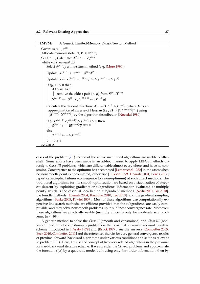
2.2. Relevant Existing Approaches 37
LMVM: A Generic Limited-Memory Quasi-Newton Method
Given: m > 0, x(0).Allocate memory slots: S,Y ∈ Rn×m,Set k ← 0, Calculate: d(k) ← −∇f (k)
while not converged doSelect β(k) by a line-search method (e.g, [More 1994])
Update: x(k+1) ← x(k) + β(k)d(k)
Update: s← x(k+1) − x(k), y ← ∇f (k+1) −∇f (k)
if 〈y, s〉 > 0 thenif k > m then
remove the oldest pair s,y from S(k),Y (k)
S(k+1) ← [S(k) s]; Y (k+1) ← [Y (k) y]
Calculate the descent direction: d = −H(k+1)∇f (k+1), whereH is anapproximation of inverse of Hessian (i.e.,H ≈ [∇2f (k+1)]−1) usingS(k+1),Y (k+1) by the algorithm described in [Nocedal 1980]
if 〈−H(k+1)∇f (k+1),∇f (k+1)〉 > 0 thend(k+1) ← −H(k+1)∇f (k+1)
elsed(k+1) ← −∇f (k+1)
k ← k + 1return x
cases of the problem (2.1). None of the above mentioned algorithms are usable off-the-shelf. Some efforts have been made in an ad-hoc manner to apply LBFGS methods di-rectly to Class-III problems, which are differentiable almost everywhere, and have no con-straint. Convergence to the optimum has been noted [Lemaréchal 1982] in the cases whenno nonsmooth point is encountered, otherwise [Luksan 1999, Haarala 2004, Lewis 2012]report catastrophic failures (convergence to a non-optimum) of such direct methods. Thetraditional algorithms for nonsmooth optimization are based on a stabilization of steep-est descent by exploiting gradients or subgradients information evaluated at multiplepoints, which is the essential idea behind subgradient methods [Nedic 2001, Yu 2010],the bundle methods [Haarala 2004, Karmitsa 2010, Teo 2010], and the gradient samplingalgorithms [Burke 2005, Kiwiel 2007]. Most of these algorithms use computationally ex-pensive line-search methods, are efficient provided that the subgradients are easily com-putable, and they solve nonsmooth problems up to sublinear convergence rate. Moreover,these algorithms are practically usable (memory efficient) only for moderate size prob-lems, (n ≤ 105).
A generic method to solve the Class-II (smooth and constrained) and Class-III (non-smooth and may be constrained) problems is the proximal forward-backward iterativescheme introduced in [Passty 1979] and [Bruck 1977]; see the surveys [Combettes 2005,Beck 2010, Combettes 2011] and the references therein for very general convergence resultsof proximal forward-backward algorithms under various conditions and settings relevantto problem (2.1). Here, I revise the concept of two very related algorithms in the proximalforward-backward iterative scheme. If we consider the Class-II problem, and approximatethe function f(x) by a quadratic model built using only first-order information, then by
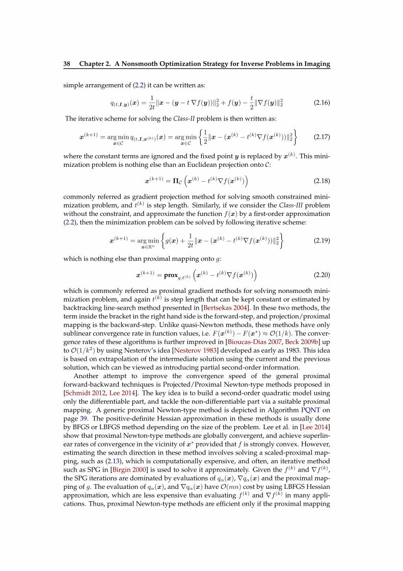
38 Chapter 2. A Nonsmooth Optimization Strategy for Inverse Problems in Imaging
simple arrangement of (2.2) it can be written as:
q(t,I,y)(x) =1
2t‖x− (y − t∇f(y))‖22 + f(y)− t
2‖∇f(y)‖22 (2.16)
The iterative scheme for solving the Class-II problem is then written as:
x(k+1) = arg minx∈C
q(t,I,x(k))(x) = arg minx∈C
1
2‖x− (x(k) − t(k)∇f(x(k)))‖22
(2.17)
where the constant terms are ignored and the fixed point y is replaced by x(k). This mini-mization problem is nothing else than an Euclidean projection onto C:
x(k+1) = ΠC
(x(k) − t(k)∇f(x(k))
)(2.18)
commonly referred as gradient projection method for solving smooth constrained mini-mization problem, and t(k) is step length. Similarly, if we consider the Class-III problemwithout the constraint, and approximate the function f(x) by a first-order approximation(2.2), then the minimization problem can be solved by following iterative scheme:
x(k+1) = arg minx∈Rn
g(x) +
1
2t‖x− (x(k) − t(k)∇f(x(k)))‖22
(2.19)
which is nothing else than proximal mapping onto g:
x(k+1) = proxg,t(k)(x(k) − t(k)∇f(x(k))
)(2.20)
which is commonly referred as proximal gradient methods for solving nonsmooth mini-mization problem, and again t(k) is step length that can be kept constant or estimated bybacktracking line-search method presented in [Bertsekas 2004]. In these two methods, theterm inside the bracket in the right hand side is the forward-step, and projection/proximalmapping is the backward-step. Unlike quasi-Newton methods, these methods have onlysublinear convergence rate in function values, i.e. F (x(k))−F (x∗) ≈ O(1/k). The conver-gence rates of these algorithms is further improved in [Bioucas-Dias 2007, Beck 2009b] uptoO(1/k2) by using Nesterov’s idea [Nesterov 1983] developed as early as 1983. This ideais based on extrapolation of the intermediate solution using the current and the previoussolution, which can be viewed as introducing partial second-order information.
Another attempt to improve the convergence speed of the general proximalforward-backward techniques is Projected/Proximal Newton-type methods proposed in[Schmidt 2012, Lee 2014]. The key idea is to build a second-order quadratic model usingonly the differentiable part, and tackle the non-differentiable part via a suitable proximalmapping. A generic proximal Newton-type method is depicted in Algorithm PQNT onpage 39. The positive-definite Hessian approximation in these methods is usually doneby BFGS or LBFGS method depending on the size of the problem. Lee et al. in [Lee 2014]show that proximal Newton-type methods are globally convergent, and achieve superlin-ear rates of convergence in the vicinity of x∗ provided that f is strongly convex. However,estimating the search direction in these method involves solving a scaled-proximal map-ping, such as (2.13), which is computationally expensive, and often, an iterative methodsuch as SPG in [Birgin 2000] is used to solve it approximately. Given the f (k) and ∇f (k),the SPG iterations are dominated by evaluations of qα(x), ∇qα(x) and the proximal map-ping of g. The evaluation of qα(x), and ∇qα(x) have O(mn) cost by using LBFGS Hessianapproximation, which are less expensive than evaluating f (k) and ∇f (k) in many appli-cations. Thus, proximal Newton-type methods are efficient only if the proximal mapping

2.2. Relevant Existing Approaches 39
of g is not expensive. In overall, proximal Newton-type methods are computationallymore expensive than quasi-Newton methods per iteration; indeed they require to solvea similar type of optimization problem twice per iteration. In our experiments, we com-pare the convergence time of proximal Newton-type method (particularly minConf_QNSTin [Schmidt 2012]) with variants of ADMM (what is discussed next), and our proposedalgorithm, and find that the proximal Newton-type method is significantly slower thanADMM and our proposed algorithm.
PQNT: A Generic Proximal Newton-type Method [Schmidt 2012, Lee 2014]
Given: x(0) ∈ dom f , set k ← 0
while not converged doif ‖ proxg,1
(x(k) −∇f (k)
)− x(k)‖ ≤ ε then
Converged
Choose a positive definite B(k) ≈ ∇2f (k)
Build local quadratic model:qα(x,x(k)) = f (k) + (x− x(k))∇f (k) + 1
2α (x− x(k))TB(k)(x− x(k)) + g(x)
Solve the subproblem for a search direction:
x(k) = arg minx
qα(x,x(k)) = proxg,α,B(x(k) − α[B(k)]−1∇f (k)
)d(k) ← x(k) − x(k)
Select β(k) with backtracking line-search such as described in [Bertsekas 2004]
Update: x(k+1) ← x(k) + β(k)d(k)
k ← k + 1return x
A similar attempt to accelerate the general forward-backward techniques for solvingClass-III problems is proposed in [Chouzenoux 2014], where that variable metric (approxi-mation of inverse of Hessian) is built using Majorization-Minimization strategy. The com-putational expense per iteration for this method is similar to the proximal Newton-typemethods in [Schmidt 2012, Lee 2014] and has been shown to be faster than acceleratedproximal gradient methods(using Nesterov’s idea) on some image restoration problems.The step-size in this method is kept fixed and chosen manually for the fast convergence.
Other instances of the general proximal forward-backward iterative scheme are the Al-ternating Minimization Algorithm in [Tseng 1991], and Alternating Direction Method ofMultipliers (ADMM) proposed in [Gabay 1976], which are closely related to algorithmssuch as dual decomposition, the method of multipliers, Douglas-Rachford splittings, Dyk-stra’s alternating projections, split Bregman iterative method, and others; see the mono-graph [Boyd 2011] for general perspectives and applications. These algorithms are basedon the idea of variable splitting and augmented Lagrangian to handle the constraints.
For the sake of completeness, before proceeding to the description of the method of multi-pliers and the ADMM, we review the concept of Lagrangian and augmented Lagrangianon which both the method of multipliers and the ADMM are built on. Introducing a vari-able splitting, z = x, the problem (2.1) can be equivalently written into a constrained
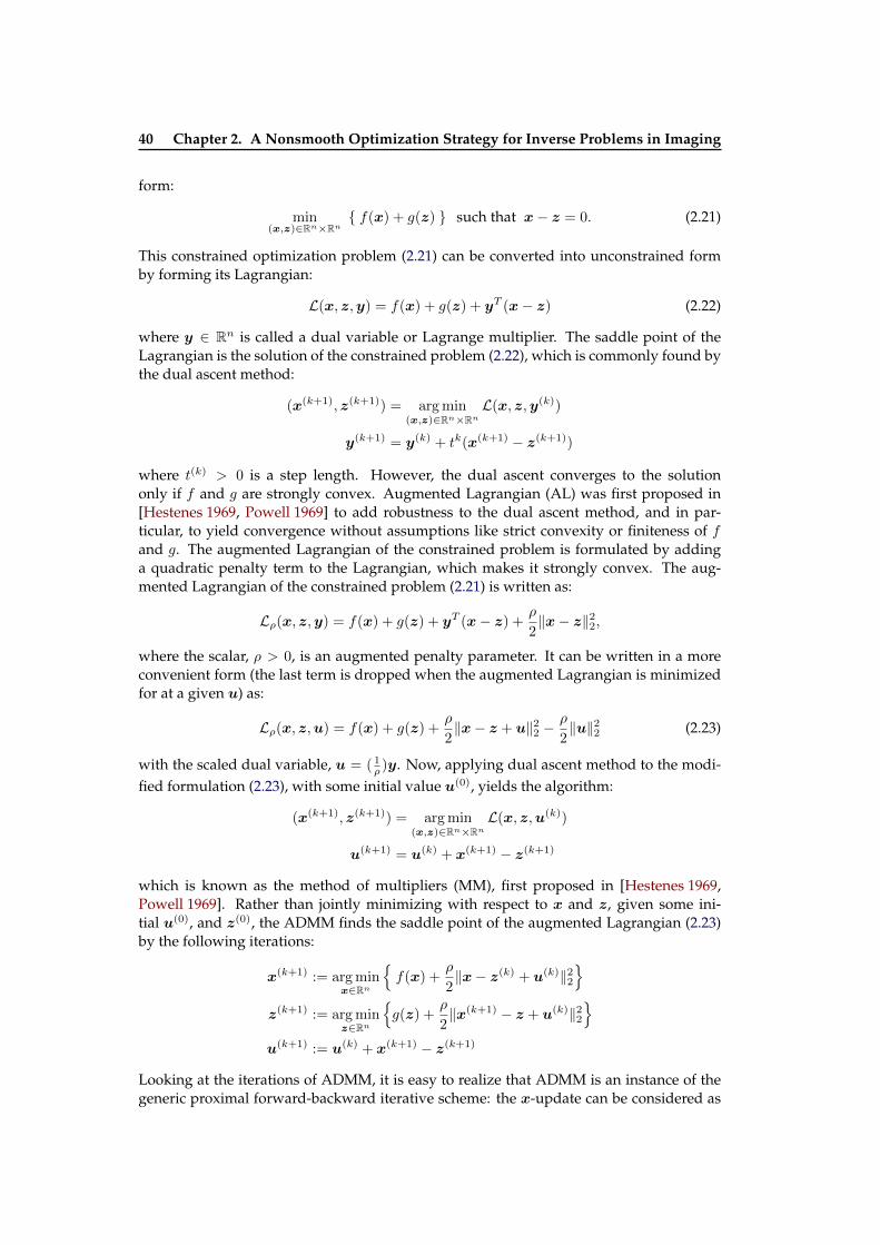
40 Chapter 2. A Nonsmooth Optimization Strategy for Inverse Problems in Imaging
form:
min(x,z)∈Rn×Rn
f(x) + g(z) such that x− z = 0. (2.21)
This constrained optimization problem (2.21) can be converted into unconstrained formby forming its Lagrangian:
L(x, z,y) = f(x) + g(z) + yT (x− z) (2.22)
where y ∈ Rn is called a dual variable or Lagrange multiplier. The saddle point of theLagrangian is the solution of the constrained problem (2.22), which is commonly found bythe dual ascent method:
(x(k+1), z(k+1)) = arg min(x,z)∈Rn×Rn
L(x, z,y(k))
y(k+1) = y(k) + tk(x(k+1) − z(k+1))
where t(k) > 0 is a step length. However, the dual ascent converges to the solutiononly if f and g are strongly convex. Augmented Lagrangian (AL) was first proposed in[Hestenes 1969, Powell 1969] to add robustness to the dual ascent method, and in par-ticular, to yield convergence without assumptions like strict convexity or finiteness of fand g. The augmented Lagrangian of the constrained problem is formulated by addinga quadratic penalty term to the Lagrangian, which makes it strongly convex. The aug-mented Lagrangian of the constrained problem (2.21) is written as:
Lρ(x, z,y) = f(x) + g(z) + yT (x− z) +ρ
2‖x− z‖22,
where the scalar, ρ > 0, is an augmented penalty parameter. It can be written in a moreconvenient form (the last term is dropped when the augmented Lagrangian is minimizedfor at a given u) as:
Lρ(x, z,u) = f(x) + g(z) +ρ
2‖x− z + u‖22 −
ρ
2‖u‖22 (2.23)
with the scaled dual variable, u = ( 1ρ )y. Now, applying dual ascent method to the modi-
fied formulation (2.23), with some initial value u(0), yields the algorithm:
(x(k+1), z(k+1)) = arg min(x,z)∈Rn×Rn
L(x, z,u(k))
u(k+1) = u(k) + x(k+1) − z(k+1)
which is known as the method of multipliers (MM), first proposed in [Hestenes 1969,Powell 1969]. Rather than jointly minimizing with respect to x and z, given some ini-tial u(0), and z(0), the ADMM finds the saddle point of the augmented Lagrangian (2.23)by the following iterations:
x(k+1) := arg minx∈Rn
f(x) +
ρ
2‖x− z(k) + u(k)‖22
z(k+1) := arg min
z∈Rn
g(z) +
ρ
2‖x(k+1) − z + u(k)‖22
u(k+1) := u(k) + x(k+1) − z(k+1)
Looking at the iterations of ADMM, it is easy to realize that ADMM is an instance of thegeneric proximal forward-backward iterative scheme: the x-update can be considered as

2.3. Proposed Algorithm 41
the forward-step, and the z-update as the backward-step. ADMM and the method of mul-tipliers are quite similar except that ADMM separates the minimization over x and z intotwo steps. In fact, ADMM is viewed as a version of the method of multipliers where asingle Gauss-Seidel iteration over x and z is used instead of the usual joint minimization.The ADMM is a blend of decomposability of dual ascent and superior convergence prop-erties of the method of multipliers. Because of its flexibility to handle a variety of objec-tive functions/constraints, and its simplicity in implementation for distributed optimiza-tion, ADMM has gained a large popularity among both the signal processing and machinelearning communities, since the last few decades. The advantage of the two methods: themethod of multipliers and ADMM, is their guaranteed convergence to the solution undervery mild assumptions:
1. The real-valued functions f and g are closed, proper, and convex.
2. The Lagrangian L0 has a saddle point.
See [Bertsekas 1976, Gabay 1983, Eckstein 1992, Boyd 2011] for general convergence dis-cussion of ADMM. Assumption 1 implies that the subproblem(s) arising in the x and z-update is(are) solvable, i.e., there exists x and z, not necessarily unique (without furtherassumptions), that minimize the augmented Lagrangian. Assumption 2 implies that thereexists (x∗, z∗,y∗), for which
L0(x∗, z∗,y) ≤ L0(x∗, z∗,y∗) ≤ L0(x, z,y∗)
hold for all x, z, y. By assumption 1, it follows that L0(x∗, z∗,y∗) is finite for any saddlepoint (x∗, z∗,y∗), which implies that (x∗, z∗) is the solution of constrained problem (2.21).One more advantage of these methods is that they do converge even when the x andz-updates are not carried out exactly (it is the cases when the updates do not have closed-form solutions, and are estimated by some iterative methods), provided that the `2-normof the errors between the exact and approximate updates at each iteration are summable,see [Eckstein 1992] for the proof.
Like the other algorithms in proximal forward-backward iterative schemes, ADMMcan achieve sublinear convergence rate under the stated assumptions. However, the au-thors in [Afonso 2010a, Afonso 2010b, Afonso 2011, Matakos 2013] show experimentallythat ADMM converges faster than many other algorithms in the general proximal forward-backward iterative scheme provided that it decomposes the problem into multiple sub-problems such that each of them can be solved exactly (in closed-form), and all the penaltyparameters associated with the augmented terms are tuned optimally. However, the op-timal tuning of the involved penalty parameters is still an open challenge; in our experi-mental results we will see that the convergence speed of ADMM is very sensitive to thevariation in the penalty parameters.
2.3 Proposed Algorithm
2.3.1 Motivation and Contributions
Motivation: As pointed out in the preceding section 2.2, the algorithms based on the gen-eral proximal forward-backward iterative scheme are good candidates for solving largesize constrained nonsmooth problems like (2.1). Among them, the accelerated proxi-mal gradient methods (e.g., MFISTA in [Beck 2009a, Beck 2009b]), the proximal Newton-type method (e.g., minConf_PQN, minConf_QNST in [Schmidt 2009, Schmidt 2012],
42 Chapter 2. A Nonsmooth Optimization Strategy for Inverse Problems in Imaging
and [Lee 2014]), and variants of ADMM (e.g., SALSA in [Afonso 2010a], C-SALSA in[Afonso 2011], and [Matakos 2013]) are notable state-of-the-art algorithms for solving theproblems (2.1) in signal/image processing and machine learning. Recently proposed vari-ants of ADMM [Afonso 2010a, Afonso 2011, Matakos 2013] have shown to outperformthe accelerated proximal gradient methods in [Becker 2011, Bioucas-Dias 2007, Beck 2009a,Beck 2009b] in term of convergence speed for solving the instances of the general problem(2.1) in applications related to image restoration, and other linear inverse problems. Lee etal. show in [Lee 2014] that proximal Newton-type methods achieve a fast convergence ratein the vicinity of the optimal solution under the assumption that the function f is stronglyconvex. In many practical applications, it is rarely necessary to reach the exact optimal so-lution, and, moreover, the function f is not always strongly convex (we will see in Section2.4 that some image restoration problems are not strongly convex). In our experimentalresults, I compare the convergence speed of the minConf_QNST with a variant of ADMMfor image restoration problem, and find that the ADMM outperforms the minConf_QNSTby a large margin (time). With these observations, we can conclude that certain variantsof ADMM are the most efficient candidates for solving the generic problem (2.1). The ex-perimental results in [Afonso 2010b, Matakos 2013] clearly demonstrate that the variantsof ADMM converge faster than other variants, given that:
1. a sufficient number of variable splittings are introduced so that each variable updatecan be carried out in closed-form, and
2. separately optimally tuned augmented penalty parameters are used.
Unfortunately, there does not exist a universal method for optimal tuning of the aug-mented penalty parameters, and a nonoptimal tuning of the augmented penalty param-eters significantly degrades the convergence speed of ADMM. Though, the authors in[Afonso 2010b, Matakos 2013] suggest some thumb-rules to tune the parameters, but theserules cannot be generalized (in fact, their thumb-rules are efficient only on the particularproblem they try to solve in their papers) since the optimal value of the penalty parameterdepends on the scale of the data, and the specific (particularly regularization) parametersin the problem. Keeping this in mind, a nonsmooth constrained convex problem such asimage deblurring problem with total variation (TV) regularization, as the one consideredin Section 2.4.1, requires multiple variable splittings, which may result in significantlyslower convergence speed in lack of optimal tuning of the multiple parameters. Later, inSection (2.5.3), I will discuss about the need for separate penalty parameters for higherconvergence rate.Contributions: In this chapter, I propose a class of algorithms for solving a nonsmoothconstrained convex optimization problem based on the variable splitting trick and aug-mented Lagrangian similar to ADMM. The proposed algorithms is an instance of themethod of multipliers, where the joint optimization is tackled by hierarchical optimizationstrategy. The joint optimization is carried out using robust and well established limited-memory quasi-Newton method (e.g., BLMVM) in conjunction with proximal operator fornonsmooth part in the optimization problem. The use of quasi-Newton method avoidsthe requirement of multiple variable splittings. Experimentally, I show that the conver-gence speed of ADMM is highly dependent on the involved penalty parameters, whereasthe proposed algorithms involve fewer tunable parameters, are as fast as the variants ofADMM in [Afonso 2010a, Afonso 2010b, Afonso 2011, Matakos 2013], and with a conver-gence speed almost insensitive to large variations in the penalty parameters.

2.3. Proposed Algorithm 43
2.3.2 Basic Ingredients
The proposed algorithm for nonsmooth constrained convex optimization problem isbased on the variable splitting trick, and on the augmented Lagrangian. It is an instanceof the method of multipliers, where the joint optimization is tackled by hierarchicaloptimization strategy, and the nonsmoothness by proximal mapping. To avoid multiplevariable splittings, and for other advantages (that we will see), limited-memory quasi-Newton method is used for the joint optimization. Before proceeding further into thedetails of the proposed algorithm, I recall here its basic ingredients.
Variable Splitting, Augmented Lagrangian, and the Method of Multipliers: In order todecouple the smooth part and the nonsmooth part of the generic problem (2.1), a variablesplitting is introduced, and the equivalent problem is written into a constrained form:
min(x,z)∈Rn×Rn
f(x) + g(z) such that x− z = 0. (2.24)
This constrained problem (2.24) is converted into an unconstrained form by the aug-mented Lagrangian technique, and is written as:
Lρ(x, z,u) = f(x) + g(z) +ρ
2‖x− z + u‖22 −
ρ
2‖u‖22 (2.25)
where ρ > 0 is an augmented penalty parameter, and u is scaled dual variable. The saddlepoint of the augmented Lagrangian (2.25) is the solution to the constrained problem (2.24).This saddle point is found by the method of multipliers whose iterations are:
x(k+1), z(k+1) = arg min(x,z)∈Rn×Rn
f(x) + g(z) +
ρ
2‖x− z + u(k)‖22
(2.26)
u(k+1) = u(k) + x(k+1) − z(k+1) (2.27)
The optimization problem (2.26) is almost as difficult as the main problem (2.1). Inthe proposed algorithm, this is solved by the limited-memory quasi-Newton method inconjunction with proximal mapping for the nonsmooth part. Let me now present thequasi-Newton method that I have used in my work.
Limited Memory Quasi-Newton Method for Smooth Bound Constrained Optimization:As mentioned earlier, there are several efficient algorithms (e.g., LBFGS-B, VMLM-B,BLMVM, minConf_TMP) for solving the large-scale Class-II (smooth and constrained)problems when C = x : l ≤ x ≤ u, is a simple bounded constraint set. In the proposedalgorithm, I use the BLMVM 2. Like other quasi-Newton methods, BLMVM is based onquadratic approximation (2.2) of the function f at the current iteration, which gives thedescent direction d = −[B(k)]−1∇f(x(k)), where B(k) is positive definite approximationof the Hessian. The Hessian is approximated by LBFGS method using only m, (m n),correction pairs (s,y). Unlike LBFGS-B, the BLMVM uses projected gradient, defined as:
T (∇f(x),x) =
(∇f(x))i if xi ∈ (li,ui)
min(∇f(x))i, 0 if xi = limax(∇f(x))i, 0 if xi = ui
in LBFGS matrix update instead of normal gradient, where l and u are lower and upperbounds. It is easy to see that the restricted variables set with indices given by
B(x) = i : xi = li and (∇f(x))i ≥ 0, or xi = ui and (∇f(x))i ≤ 02An open source implementation of BLMVM, VMLM-B and other optimization algorithms are available at
https://github.com/emmt/OptimPack.
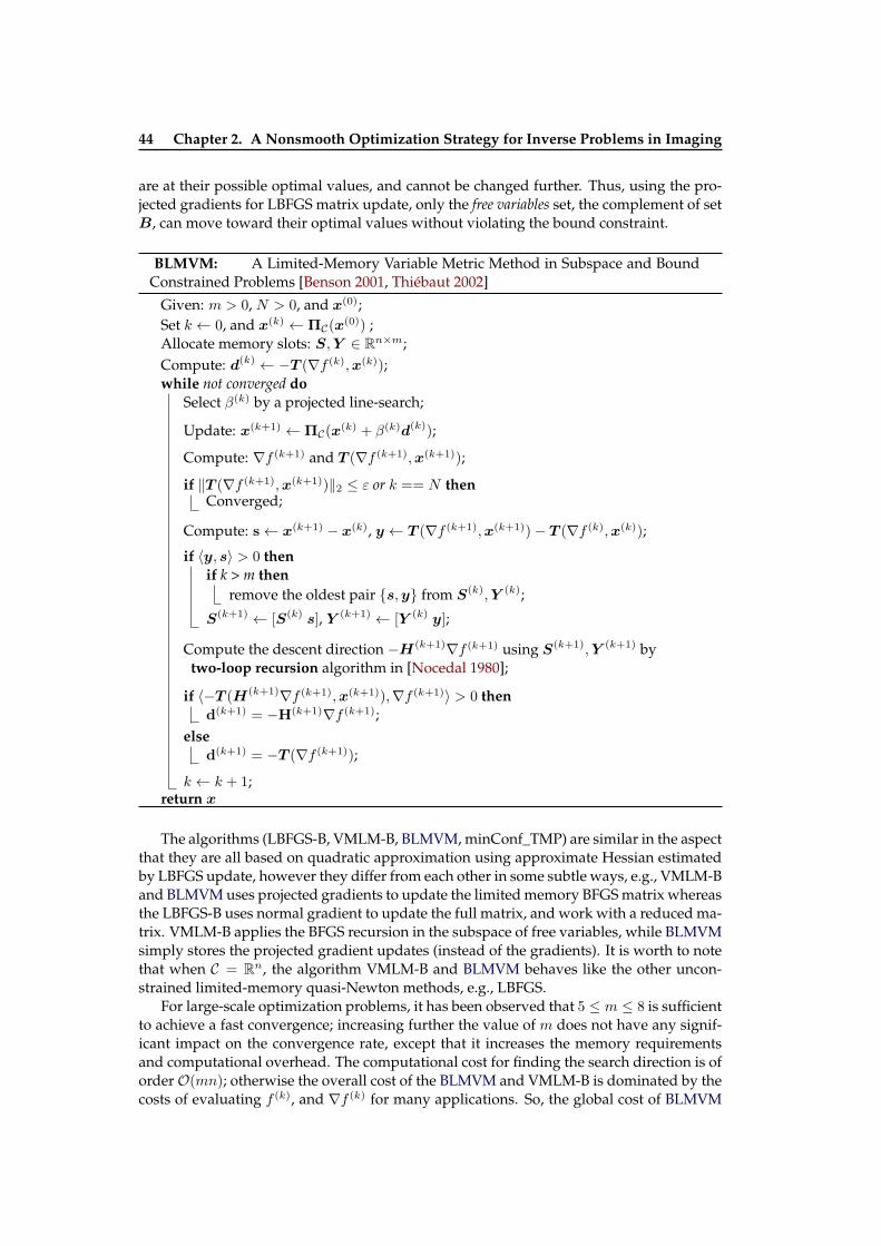
44 Chapter 2. A Nonsmooth Optimization Strategy for Inverse Problems in Imaging
are at their possible optimal values, and cannot be changed further. Thus, using the pro-jected gradients for LBFGS matrix update, only the free variables set, the complement of setB, can move toward their optimal values without violating the bound constraint.
BLMVM: A Limited-Memory Variable Metric Method in Subspace and BoundConstrained Problems [Benson 2001, Thiébaut 2002]
Given: m > 0, N > 0, and x(0);Set k ← 0, and x(k) ← ΠC(x
(0)) ;Allocate memory slots: S,Y ∈ Rn×m;Compute: d(k) ← −T (∇f (k),x(k));while not converged do
Select β(k) by a projected line-search;
Update: x(k+1) ← ΠC(x(k) + β(k)d(k));
Compute: ∇f (k+1) and T (∇f (k+1),x(k+1));
if ‖T (∇f (k+1),x(k+1))‖2 ≤ ε or k == N thenConverged;
Compute: s← x(k+1) − x(k), y ← T (∇f (k+1),x(k+1))− T (∇f (k),x(k));
if 〈y, s〉 > 0 thenif k > m then
remove the oldest pair s,y from S(k),Y (k);
S(k+1) ← [S(k) s], Y (k+1) ← [Y (k) y];
Compute the descent direction −H(k+1)∇f (k+1) using S(k+1),Y (k+1) bytwo-loop recursion algorithm in [Nocedal 1980];
if 〈−T (H(k+1)∇f (k+1),x(k+1)),∇f (k+1)〉 > 0 thend(k+1) = −H(k+1)∇f (k+1);
elsed(k+1) = −T (∇f (k+1));
k ← k + 1;return x
The algorithms (LBFGS-B, VMLM-B, BLMVM, minConf_TMP) are similar in the aspectthat they are all based on quadratic approximation using approximate Hessian estimatedby LBFGS update, however they differ from each other in some subtle ways, e.g., VMLM-Band BLMVM uses projected gradients to update the limited memory BFGS matrix whereasthe LBFGS-B uses normal gradient to update the full matrix, and work with a reduced ma-trix. VMLM-B applies the BFGS recursion in the subspace of free variables, while BLMVMsimply stores the projected gradient updates (instead of the gradients). It is worth to notethat when C = Rn, the algorithm VMLM-B and BLMVM behaves like the other uncon-strained limited-memory quasi-Newton methods, e.g., LBFGS.
For large-scale optimization problems, it has been observed that 5 ≤ m ≤ 8 is sufficientto achieve a fast convergence; increasing further the value of m does not have any signif-icant impact on the convergence rate, except that it increases the memory requirementsand computational overhead. The computational cost for finding the search direction is oforderO(mn); otherwise the overall cost of the BLMVM and VMLM-B is dominated by thecosts of evaluating f (k), and ∇f (k) for many applications. So, the global cost of BLMVM
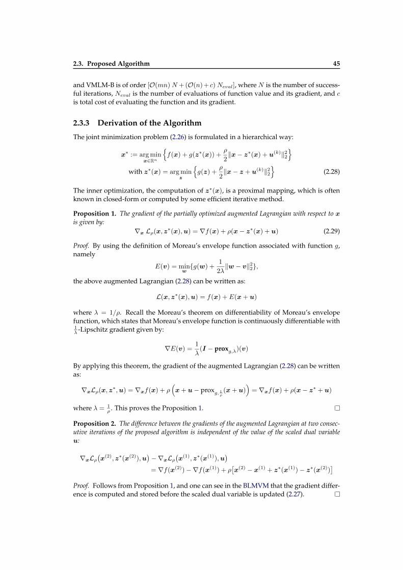
2.3. Proposed Algorithm 45
and VMLM-B is of order [O(mn)N + (O(n) + c)Neval], where N is the number of success-ful iterations, Neval is the number of evaluations of function value and its gradient, and c
is total cost of evaluating the function and its gradient.
2.3.3 Derivation of the Algorithm
The joint minimization problem (2.26) is formulated in a hierarchical way:
x∗ := arg minx∈Rn
f(x) + g(z∗(x)) +
ρ
2‖x− z∗(x) + u(k)‖22
with z∗(x) = arg min
z
g(z) +
ρ
2‖x− z + u(k)‖22
(2.28)
The inner optimization, the computation of z∗(x), is a proximal mapping, which is oftenknown in closed-form or computed by some efficient iterative method.
Proposition 1. The gradient of the partially optimized augmented Lagrangian with respect to xis given by:
∇x Lρ(x, z∗(x),u) = ∇f(x) + ρ(x− z∗(x) + u) (2.29)
Proof. By using the definition of Moreau’s envelope function associated with function g,namely
E(v) = minwg(w) +
1
2λ‖w − v‖22,
the above augmented Lagrangian (2.28) can be written as:
L(x, z∗(x),u) = f(x) + E(x+ u)
where λ = 1/ρ. Recall the Moreau’s theorem on differentiability of Moreau’s envelopefunction, which states that Moreau’s envelope function is continuously differentiable with1λ -Lipschitz gradient given by:
∇E(v) =1
λ(I − proxg,λ)(v)
By applying this theorem, the gradient of the augmented Lagrangian (2.28) can be writtenas:
∇xLρ(x, z∗,u) = ∇xf(x) + ρ(x+ u− proxg, 1ρ (x+ u)
)= ∇xf(x) + ρ(x− z∗ + u)
where λ = 1ρ . This proves the Proposition 1.
Proposition 2. The difference between the gradients of the augmented Lagrangian at two consec-utive iterations of the proposed algorithm is independent of the value of the scaled dual variableu:
∇xLρ(x(2), z∗(x(2)),u
)−∇xLρ
(x(1), z∗(x(1)),u
)= ∇f(x(2))−∇f(x(1)) + ρ
[x(2) − x(1) + z∗(x(1))− z∗(x(2))
]Proof. Follows from Proposition 1, and one can see in the BLMVM that the gradient differ-ence is computed and stored before the scaled dual variable is updated (2.27).
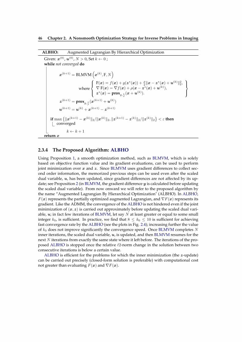
46 Chapter 2. A Nonsmooth Optimization Strategy for Inverse Problems in Imaging
ALBHO: Augmented Lagrangian By Hierarchical Optimization
Given: x(0), u(0), N > 0, Set k ← 0 ;while not converged do
x(k+1) = BLMVM(x(k),F, N
)where
F(x) = f(x) + g(z∗(x)) + ρ
2‖x− z∗(x) + u(k)‖22,∇ F(x) = ∇f(x) + ρ(x− z∗(x) + u(k)),
z∗(x) = proxg, 1ρ (x+ u(k)).
z(k+1) = proxg, 1ρ (x(k+1) + u(k))
u(k+1) = u(k) + x(k+1) − z(k+1)
if max‖x(k+1) − x(k)‖2/‖x(k)‖2, ‖z(k+1) − z(k)‖2/‖z(k)‖2
< ε then
converged
k ← k + 1return x
2.3.4 The Proposed Algorithm: ALBHO
Using Proposition 1, a smooth optimization method, such as BLMVM, which is solelybased on objective function value and its gradient evaluations, can be used to performjoint minimization over x and z. Since BLMVM uses gradient differences to collect sec-ond order information, the memorized previous steps can be used even after the scaleddual variable, u, has been updated, since gradient differences are not affected by its up-date; see Proposition 2 (in BLMVM, the gradient difference y is calculated before updatingthe scaled dual variable). From now onward we will refer to the proposed algorithm bythe name “Augmented Lagrangian By Hierarchical Optimization" (ALBHO). In ALBHO,F (x) represents the partially optimized augmented Lagrangian, and∇F (x) represents itsgradient. Like the ADMM, the convergence of the ALBHO is not hindered even if the jointminimization of (x, z) is carried out approximately before updating the scaled dual vari-able, u; in fact few iterations of BLMVM, let say N at least greater or equal to some smallinteger k0, is sufficient. In practice, we find that 8 ≤ k0 ≤ 10 is sufficient for achievingfast convergence rate by the ALBHO (see the plots in Fig. 2.4); increasing further the valueof k0 does not improve significantly the convergence speed. Once BLMVM completes Ninner iterations, the scaled dual variable, u, is updated, and then BLMVM resumes for thenext N iterations from exactly the same state where it left before. The iterations of the pro-posed ALBHO is stopped once the relative `2-norm change in the solution between twoconsecutive iterations is below a certain value.
ALBHO is efficient for the problems for which the inner minimization (the z-update)can be carried out precisely (closed-form solution is preferable) with computational costnot greater than evaluating F (x) and ∇F (x).

2.4. Comparison of ALBHO with State-Of-The-Art Algorithms 47
2.4 Comparison of ALBHO with State-Of-The-Art Algo-rithms
As pointed out in section 2.2, variants of ADMM have been proven to be fast and efficientstate-of-the-art algorithms for solving constrained convex nonsmooth optimization prob-lems in signal/image processing, and computer vision. Thus, to demonstrate the advan-tages and the performance of the proposed ALBHO over the ADMM, I consider some ofthe vastly investigated problems in image processing and computer vision. The first prob-lem (Problem 1) is image deblurring with TV and positivity constraint in which the data-fidelity term is quadratic. The second problem (Problem 2) is Poissonian image deblurringwith TV and positivity in which the data-fidelity term is not quadratic, but contains a log-arithmic term. The third problem (Problem 3) is globally convex image segmentation, inwhich the data-fidelity term is linear. Two more image deblurring problems are consid-ered for comparison with proximal Newton-type method, which are slightly different inorder to show that the ALBHO is applicable to a wide range of optimization problemsarising in imaging, and it is as fast as other state-of-the-art algorithms, but without anyparameter tuning. The problems and the algorithms are presented in what follows.
2.4.1 Problem 1: Image Deblurring with TV and Positivity Constraint
The first problem considered for the illustration is shift-invariant image deblurring withtotal variation (TV) regularization and positivity constraint, stated as:
x∗ := arg minx∈Rn
1
2‖y −Hx‖2W + ιC(x) + λ TV(x)
(2.30)
where y is the blurry and noisy image obtained from the crisp image x after applying thediscrete blurring operatorH , and corrupting it with Gaussian noise. It is often efficient toapply the blurring operator in Fourier domain using fast Fourier transform (FFT) as de-scribed in Section 1.3.1 in Chapter 1. Note that the two dimensional image matrix is repre-sented by a column vector by lexicographically ordering its pixels. The set C = x : x ≥ 0represents the set of vectors in the positive-orthant. The regularization parameter λ > 0
is tuned to reach a good compromise between the likelihood data-fidelity and the priorregularizer, TV(x) the isotropic total variation defined as: TV(x) =
∑i ‖(Dx)i‖2, where
Dx ∈ Rn×2, and D = [DT(1),D
T(2)]
T is the circular first-order finite difference operator intwo dimensions. As discussed in [Matakos 2013], due the circular blurring operator, thedeblurred image suffers from wraparound artifact along the boundary. The wraparoundartifact come from the implied periodicity of the circular blurring operator. Thus, to han-dle this problem, a weighted least-square likelihood term is considered, a similar idea asin [Matakos 2013]. W is the inverse of the diagonal noise covariance matrix. The pixelsoutside the field-of-view or any unmeasured pixel (e.g. dead or saturated pixels) in theobserved image can be considered to have an infinite variance, thus, are given zero weightin matrixW (i.e. if pixel k is unmeasured, thenW (k, k) = 0). To prevent the wraparoundartifact along the boundaries of the image, we seek to reconstruct x ∈ Rn slightly largerthan the available observed image y ∈ Rm, where n > m. Thus, we extend the observedimage to new size n by zero-padding at boundaries, i.e. y ∈ Rn. Similarly, we add zerostoW for the corresponding boundary pixels.
The optimization problem (2.30) is a perfect instance of the general problem (2.1). Itinvolves a continuously differentiable data-fidelity term, a nonsmooth regularizer term,and positivity constraint. To compare the performance and advantages of the proposed
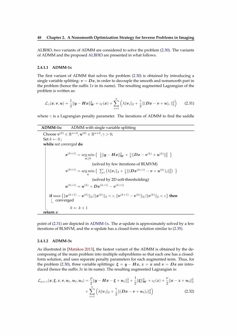
48 Chapter 2. A Nonsmooth Optimization Strategy for Inverse Problems in Imaging
ALBHO, two variants of ADMM are considered to solve the problem (2.30). The variantsof ADMM and the proposed ALBHO are presented in what follows.
2.4.1.1 ADMM-1x
The first variant of ADMM that solves the problem (2.30) is obtained by introducing asingle variable splitting: v = Dx, in order to decouple the smooth and nonsmooth part inthe problem (hence the suffix 1x in its name). The resulting augmented Lagrangian of theproblem is written as:
Lγ(x,v,u) =1
2‖y −Hx‖2W + ιC(x) +
n∑i=1
(λ‖vi‖2 +
γ
2‖(Dx− v + u)i ‖22
)(2.31)
where γ is a Lagrangian penalty parameter. The iterations of ADMM to find the saddle
ADMM-1x: ADMM with single variable splitting
Choose v(0) ∈ Rn×2,u(0) ∈ Rn×2, γ > 0;Set k ← 0 ;while not converged do
x(k+1) = arg minx≥0
12‖y −Hx‖2W + γ
2 ‖Dx− v(k) + u(k)‖22
(solved by few iterations of BLMVM)
v(k+1) = arg minv
∑i
(λ‖vi‖2 + γ
2 ‖(Dx(k+1) − v + u(k))i‖22)
(solved by 2D soft-thresholding)
u(k+1) = u(k) +Dx(k+1) − v(k+1)
if max‖x(k+1) − x(k)‖2/‖x(k)‖2 < ε, ‖v(k+1) − v(k)‖2/‖v(k)‖2 < ε
then
converged
k ← k + 1return x
point of (2.31) are depicted in ADMM-1x. The x-update is approximately solved by a fewiterations of BLMVM, and the v-update has a closed-form solution similar to (2.35).
2.4.1.2 ADMM-3x
As illustrated in [Matakos 2013], the fastest variant of the ADMM is obtained by the de-composing of the main problem into multiple subproblems so that each one has a closed-form solution, and uses separate penalty parameters for each augmented term. Thus, forthe problem (2.30), three variable splittings: ξ = y −Hx, z = x and v = Dx are intro-duced (hence the suffix 3x in its name). The resulting augmented Lagrangian is:
Lρ,ν,γ(x, ξ, z,v,u1,u2,u3) =ρ
2‖y −Hx− ξ + u1‖22 +
1
2‖ξ‖2W + ιC(z) +
ν
2‖x− z + u2‖22
+
n∑i=1
(λ‖vi‖2 +
γ
2‖(Dx− v + u3)i‖22
)(2.32)

2.4. Comparison of ALBHO with State-Of-The-Art Algorithms 49
where ρ, ν, and γ are the Lagrangian penalty parameters. The iterations are depicted inADMM-3x. The closed-form solutions for x-, ξ-, z-, and v-updates are given by:
x =(γDTD + ρHTH + νI
)−1 (γDT (v − u3) + ρHT (y − ξ + u1) + ν(z − u2)
)(2.33)
ξ = (ρI +W )−1ρ (y −Hx+ u1) (2.34)
vi =
‖ϑi‖2 −
λ
γ
+
ϑi‖ϑi‖2
,with ϑ = (Dx+ u3) (2.35)
z = x+ u2+ (2.36)
ADMM-3x: ADMM with three variable splittings
Choose ξ(0) ∈ Rn,v(0) ∈ Rn×2, z(0) ∈ Rn,u(0)1 ∈ Rn,u(0)
2 ∈ Rn,u(0)3 ∈ Rn×2, ρ, γ, ν;
Set k ← 0 ;while not converged do
x(k+1) = arg minx
ρ2‖y −Hx− ξ(k) + u
(k)1 ‖22 + ν
2‖x− z(k) + u(k)2 ‖22
+γ2 ‖Dx− v(k) + u
(k)3 ‖22
ξ(k+1) = arg min
ξ
12‖ξ‖2W + ρ
2‖y −Hx(k+1) − ξ + u(k)1 ‖22
v(k+1) = arg min
v
∑ni=1
(λ‖vi‖2 + γ
2 ‖(Dx(k+1) − v + u(k)3 )i‖22
) z(k+1) = arg min
z
g(z) + ν
2‖x(k+1) − z + u(k)2 ‖22
u
(k+1)1 = u
(k)1 + y −Hx(k+1) − ξ(k+1)
u(k+1)2 = u
(k)2 + x(k+1) − z(k+1)
u(k+1)3 = u
(k)3 +Dx(k+1) − v(k+1)
if max‖x(k+1) − x(k)‖2/‖x(k)‖2, ‖z(k+1) − z(k)‖2/‖z(k)‖2 < ε
then
converged
k ← k + 1return z
2.4.1.3 ALBHO
Similar to ADMM-1x, a single splitting: v = Dx, is introduced, and the augmented La-grangian is written exactly as in (2.31). ALBHO minimizes the augmented Lagrangian(2.31), given the two input expressions:
F(x) =
n∑i=1
(λ‖v∗i (x)‖2 +
γ
2‖(ϑ− v∗(x))i‖22
)+
1
2‖y −Hx‖2W
∇ F(x) = γ DT (ϑ− v∗(x))−HTW (y −Hx)
where v∗i (x) =
‖ϑi‖2 −
λ
γ
+
ϑi‖ϑi‖2
, and ϑ = (Dx+ u).
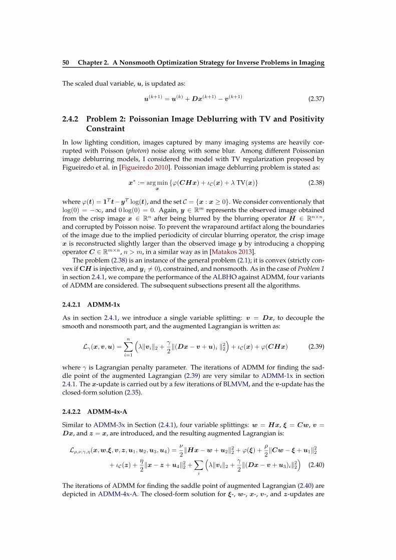
50 Chapter 2. A Nonsmooth Optimization Strategy for Inverse Problems in Imaging
The scaled dual variable, u, is updated as:
u(k+1) = u(k) +Dx(k+1) − v(k+1) (2.37)
2.4.2 Problem 2: Poissonian Image Deblurring with TV and PositivityConstraint
In low lighting condition, images captured by many imaging systems are heavily cor-rupted with Poisson (photon) noise along with some blur. Among different Poissonianimage deblurring models, I considered the model with TV regularization proposed byFigueiredo et al. in [Figueiredo 2010]. Poissonian image deblurring problem is stated as:
x∗ := arg minx
ϕ(CHx) + ιC(x) + λ TV(x) (2.38)
where ϕ(t) = 1T t−yT log(t), and the set C = x : x ≥ 0. We consider conventionaly thatlog(0) = −∞, and 0 log(0) = 0. Again, y ∈ Rm represents the observed image obtainedfrom the crisp image x ∈ Rn after being blurred by the blurring operator H ∈ Rn×n,and corrupted by Poisson noise. To prevent the wraparound artifact along the boundariesof the image due to the implied periodicity of circular blurring operator, the crisp imagex is reconstructed slightly larger than the observed image y by introducing a choppingoperator C ∈ Rm×n, n > m, in a similar way as in [Matakos 2013].
The problem (2.38) is an instance of the general problem (2.1); it is convex (strictly con-vex if CH is injective, and yi 6= 0), constrained, and nonsmooth. As in the case of Problem 1in section 2.4.1, we compare the performance of the ALBHO against ADMM, four variantsof ADMM are considered. The subsequent subsections present all the algorithms.
2.4.2.1 ADMM-1x
As in section 2.4.1, we introduce a single variable splitting: v = Dx, to decouple thesmooth and nonsmooth part, and the augmented Lagrangian is written as:
Lγ(x,v,u) =
n∑i=1
(λ‖vi‖2 +
γ
2‖(Dx− v + u)i ‖22
)+ ιC(x) + ϕ(CHx) (2.39)
where γ is Lagrangian penalty parameter. The iterations of ADMM for finding the sad-dle point of the augmented Lagrangian (2.39) are very similar to ADMM-1x in section2.4.1. The x-update is carried out by a few iterations of BLMVM, and the v-update has theclosed-form solution (2.35).
2.4.2.2 ADMM-4x-A
Similar to ADMM-3x in Section (2.4.1), four variable splittings: w = Hx, ξ = Cw, v =
Dx, and z = x, are introduced, and the resulting augmented Lagrangian is:
Lρ,ν,γ,η(x,w,ξ,v, z,u1,u2,u3,u4) =ν
2‖Hx−w + u2‖22 + ϕ(ξ) +
ρ
2‖Cw − ξ + u1‖22
+ ιC(z) +η
2‖x− z + u4‖22 +
∑i
(λ‖vi‖2 +
γ
2‖(Dx− v + u3)i‖22
)(2.40)
The iterations of ADMM for finding the saddle point of augmented Lagrangian (2.40) aredepicted in ADMM-4x-A. The closed-form solution for ξ-, w-, x-, v-, and z-updates are
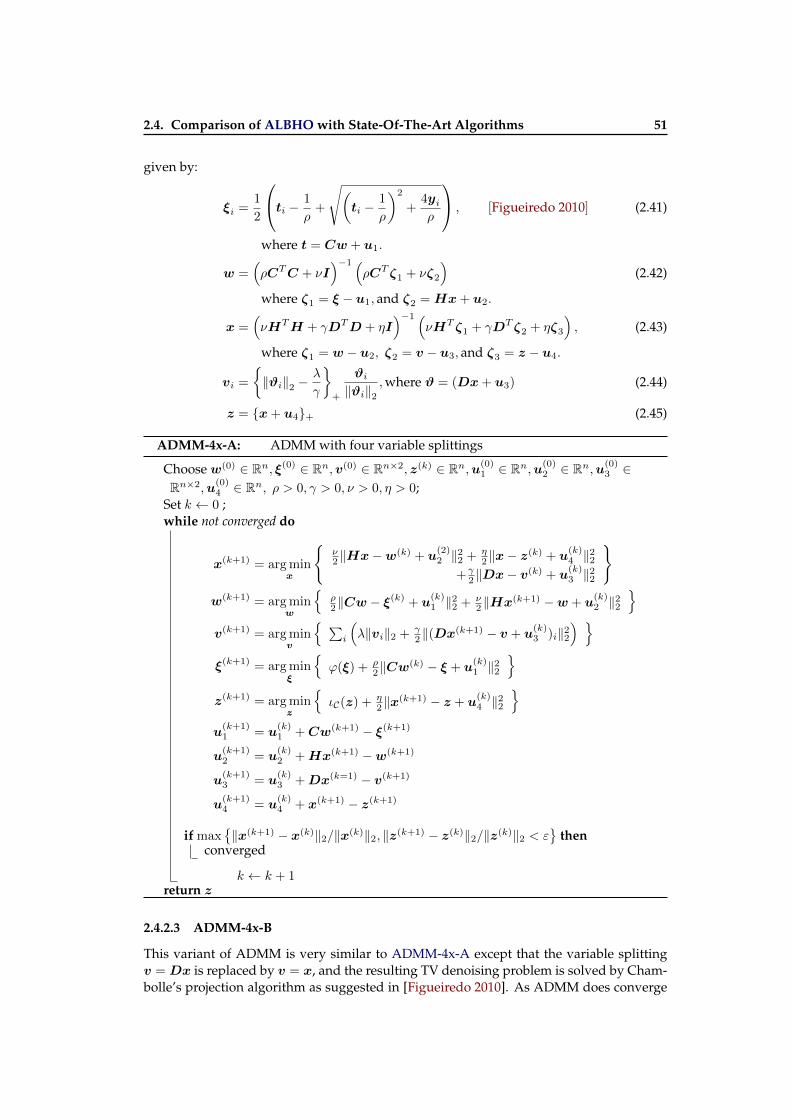
2.4. Comparison of ALBHO with State-Of-The-Art Algorithms 51
given by:
ξi =1
2
ti − 1
ρ+
√(ti −
1
ρ
)2
+4yiρ
, [Figueiredo 2010] (2.41)
where t = Cw + u1.
w =(ρCTC + νI
)−1 (ρCT ζ1 + νζ2
)(2.42)
where ζ1 = ξ − u1, and ζ2 = Hx+ u2.
x =(νHTH + γDTD + ηI
)−1 (νHT ζ1 + γDT ζ2 + ηζ3
), (2.43)
where ζ1 = w − u2, ζ2 = v − u3, and ζ3 = z − u4.
vi =
‖ϑi‖2 −
λ
γ
+
ϑi‖ϑi‖2
,where ϑ = (Dx+ u3) (2.44)
z = x+ u4+ (2.45)
ADMM-4x-A: ADMM with four variable splittings
Choose w(0) ∈ Rn, ξ(0) ∈ Rn,v(0) ∈ Rn×2, z(k) ∈ Rn,u(0)1 ∈ Rn,u(0)
2 ∈ Rn,u(0)3 ∈
Rn×2,u(0)4 ∈ Rn, ρ > 0, γ > 0, ν > 0, η > 0;
Set k ← 0 ;while not converged do
x(k+1) = arg minx
ν2‖Hx−w(k) + u
(2)2 ‖22 + η
2‖x− z(k) + u(k)4 ‖22
+γ2 ‖Dx− v(k) + u
(k)3 ‖22
w(k+1) = arg min
w
ρ2‖Cw − ξ
(k) + u(k)1 ‖22 + ν
2‖Hx(k+1) −w + u(k)2 ‖22
v(k+1) = arg min
v
∑i
(λ‖vi‖2 + γ
2 ‖(Dx(k+1) − v + u(k)3 )i‖22
) ξ(k+1) = arg min
ξ
ϕ(ξ) + ρ
2‖Cw(k) − ξ + u(k)1 ‖22
z(k+1) = arg min
z
ιC(z) + η
2‖x(k+1) − z + u(k)4 ‖22
u
(k+1)1 = u
(k)1 +Cw(k+1) − ξ(k+1)
u(k+1)2 = u
(k)2 +Hx(k+1) −w(k+1)
u(k+1)3 = u
(k)3 +Dx(k=1) − v(k+1)
u(k+1)4 = u
(k)4 + x(k+1) − z(k+1)
if max‖x(k+1) − x(k)‖2/‖x(k)‖2, ‖z(k+1) − z(k)‖2/‖z(k)‖2 < ε
then
converged
k ← k + 1return z
2.4.2.3 ADMM-4x-B
This variant of ADMM is very similar to ADMM-4x-A except that the variable splittingv = Dx is replaced by v = x, and the resulting TV denoising problem is solved by Cham-bolle’s projection algorithm as suggested in [Figueiredo 2010]. As ADMM does converge
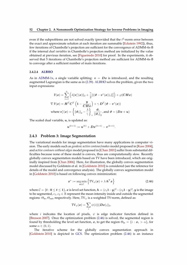
52 Chapter 2. A Nonsmooth Optimization Strategy for Inverse Problems in Imaging
even if the subproblems are not solved exactly (provided that the `2-norm error betweenthe exact and approximate solution at each iteration are summable [Eckstein 1992]), thus,few iterations of Chambolle’s projection are sufficient for the convergence of ADMM-4x-Bif the internal dual variables in Chambolle’s projection method are initialized by the valueobtained at previous iteration, see [Figueiredo 2010] for proof. In the experiments, it ob-served that 5 iterations of Chambolle’s projection method are sufficient for ADMM-4x-Bto converge after a sufficient number of main iterations.
2.4.2.4 ALBHO
As in ADMM-1x, a single variable splitting: v = Dx is introduced, and the resultingaugmented Lagrangian is the same as in (2.39). ALBHO solves the problem, given the twoinput expressions:
F(x) =
n∑i=1
(λ‖v∗i (x)‖2 +
γ
2‖(ϑ− v∗(x))i‖22
)+ ϕ(CHx)
∇ F(x) = HTCT(1− y
CHx
)+ γ DT (ϑ− v∗(x))
where v∗i (x) =
‖ϑi‖2 −
λ
γ
+
ϑi‖ϑi‖2
, and ϑ = (Dx+ u)
The scaled dual variable, u, is updated as:
u(k+1) := u(k) +Dx(k+1) − v(k+1).
2.4.3 Problem 3: Image Segmentation
The variational models for image segmentation have many applications in computer vi-sion. The early models such as geodesic active contour/snakes model proposed in [Kass 2004],and active contours without edges model proposed in [Chan 2001] suffer from substantial dif-ficulties because none of these model is convex, thus are computationally slow. Recentlyglobally convex segmentation models based on TV have been introduced, which are orig-inally inspired from [Chan 2006]. Here, for illustration, the globally convex segmentationmodel discussed by Goldstein et al. in [Goldstein 2010] is considered (see the reference fordetails of the model and convergence analysis). The globally convex segmentation modelin [Goldstein 2010] is based on following convex minimization:
x∗ := arg minx∈C
TVψ(x) + λ hTx
(2.46)
where C = t : 0 ≤ t ≤ 1, x is level set function, h = (c11−y)2−(c21−y)2, y is the imageto be segmented, c1, c2 ∈ R represent the mean intensity inside and outside the segmentedregions: Θin, Θout, respectively. Here, TVψ is a weighted TV-norm, defined as:
TVψ(x) =∑i
ψ(i)‖(Dx)i‖2,
where i indicates the location of pixels, ψ is edge indicator function defined in[Bresson 2007]. Once the optimization problem (2.46) is solved, the segmented region isfound by thresholding the level set function, x, to get the region Θin = i : xi > α, forsome α ∈ (0, 1).
The iterative scheme for the globally convex segmentation approach in[Goldstein 2010] is depicted in GCS. The optimization problem (2.46) is an instance

2.4. Comparison of ALBHO with State-Of-The-Art Algorithms 53
GCS: Globally Convex Segmentation Method [Goldstein 2010]
Initialize: c1 = 0, c2 = 0, k ← 0
while ‖x(k+1) − x(k)‖2 ≥ ε doDefine h(k) = (c
(k)1 1− y)2 − (c
(k)2 1− y)2
Solve x(k) = arg min0≤x≤1
TVψ(x) + λ (h(k))Tx
Set Θ(k)
in = i : xi > α, Θ(k)out = i : xi ≤ α
Update c(k+1)1 =
∑i∈Θin
yi, c(k+1)2 =
∑i∈Θout
yik ← k + 1
return Θin, Θout
of the general problem (2.1); it is constrained, convex and nonsmooth. With the variablesplitting: v = Dx, the augmented Lagrangian of the problem is written as:
Lρ(x,v,u) =∑i
ψ(i)‖vi‖2 +γ
2‖(Dx− v + u)i‖22 + ιC(x) + λ hTx (2.47)
The authors in [Goldstein 2010] use Split Bregman method (a variant of ADMM) to findthe saddle point of the augmented Lagrangian (2.47), where they choose a few iterationsof Gauss-Seidel method for an approximate x-update, and 2D soft-thresholding formulafor v-update, before updating the regions, (Θ
(k)in , Θ
(k)out). We find the saddle point of the
augmented Lagrangian (2.47) by a few iterations of ALBHO for which the two inputsexpressions are:
F(x) =
n∑i=1
‖v∗i (x)‖2 +γ
2‖(ϑ− v∗(x))i‖22 + λ hTx,
∇ F(x) = γDT (ϑ− v∗(x)),
where v∗i (x) =
‖ϑi‖2 −
ψ(i)
γ
+
ϑi‖ϑi‖2
, and ϑ = Dx+ u.
2.4.4 Performance Comparison of Proximal Newton-type Method vs.ADMM vs. ALBHO
Recently proposed proximal Newton-type methods are becoming popular candidates forsolving the instances of problem (2.1). Here, the performance of the proximal Newton-type method minConf_QNST proposed in [Schmidt 2012] is compared against the variantsof ADMM and the ALBHO on image restoration problems similar to the Problem 1. Thetwo image restoration problems are:
x∗ := arg minx∈Rn
1
2‖y −Hx‖2W + λ ‖x‖1
(2.48)
and
x∗ := arg minx∈Rn
1
2‖y −Hx‖2W + λ TV(x)
(2.49)
respectively, with similar notations as in problem (2.30). In order to make the problemssimple, we do not impose the positivity constraint. The variants of ADMM, the ALBHO,and minConf_QNST are presented in what follows.
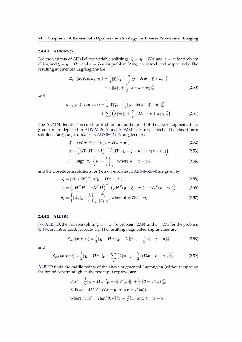
54 Chapter 2. A Nonsmooth Optimization Strategy for Inverse Problems in Imaging
2.4.4.1 ADMM-2x
For the variants of ADMM, the variable splittings: ξ = y −Hx and z = x for problem(2.48), and ξ = y −Hx and v = Dx for problem (2.49), are introduced, respectively. Theresulting augmented Lagrangians are:
Lρ,γ(x, ξ, z,u1,u2) =1
2‖ξ‖2W +
ρ
2‖y −Hx− ξ + u1‖22
+ λ ‖z‖1 +γ
2‖x− z + u2‖22 (2.50)
and
Lρ,γ(x, ξ, z,u1,u2) =1
2‖ξ‖2W +
ρ
2‖y −Hx− ξ + u1‖22
+∑i
(λ‖vi‖2 +
γ
2‖(Dx− v + u2)i‖22
)(2.51)
The ADMM iterations needed for finding the saddle point of the above augmented La-grangian are depicted in ADMM-2x-A and ADMM-2x-B, respectively. The closed-formsolutions for ξ-, x-, z-updates in ADMM-2x-A are given by:
ξ = (ρI +W )−1ρ (y −Hx+ u1) (2.52)
x =(ρHTH + γI
)−1 (ρHT (y − ξ + u1) + γ(z − u2)
)(2.53)
zi = sign(ϑi)
ϑi −
λ
γ
+
, where ϑ = x+ u2. (2.54)
and the closed-form solutions for ξ-, x-, v-updates in ADMM-2x-B are given by:
ξ = (ρI +W )−1ρ (y −Hx+ u1) (2.55)
x =(ρHTH + γDTD
)−1 (ρHT (y − ξ + u1) + γDT (v − u2)
)(2.56)
vi =
‖ϑi‖2 −
λ
γ
+
ϑi‖ϑi‖2
, where ϑ = Dx+ u2. (2.57)
2.4.4.2 ALBHO
For ALBHO, the variable splitting, z = x, for problem (2.48), and v = Dx for the problem(2.49), are introduced, respectively. The resulting augmented Lagrangians are:
Lρ,γ(x, z,u) =1
2‖y −Hx‖2W + λ ‖z‖1 +
γ
2‖x− z + u‖22 (2.58)
and
Lρ,γ(x,v,u) =1
2‖y −Hx‖2W +
∑i
(λ‖vi‖2 +
γ
2‖(Dx− v + u)i‖22
)(2.59)
ALBHO finds the saddle points of the above augmented Lagrangian (without imposingthe bound constraint) given the two input expressions:
F(x) =1
2‖y −Hx‖2W + λ‖z∗(x)‖1 +
γ
2‖ϑ− z∗(x)‖22,
∇ F(x) = HTW (Hx− y) + γ(ϑ− z∗(x)),
where z∗i (x) = sign(ϑi)|ϑi| −λ
γ+, and ϑ = x+ u.
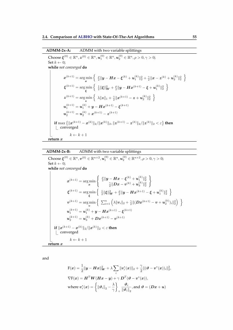
2.4. Comparison of ALBHO with State-Of-The-Art Algorithms 55
ADMM-2x-A: ADMM with two variable splittings
Choose ξ(0) ∈ Rn, z(0) ∈ Rn,u(0)1 ∈ Rn,u(0)
2 ∈ Rn, ρ > 0, γ > 0;Set k ← 0;while not converged do
x(k+1) = arg minx
ρ2‖y −Hx− ξ
(k) + u(k)1 ‖22 + γ
2 ‖x− z(k) + u(k)2 ‖22
ξ(k+1) = arg min
ξ
12‖ξ‖2W + ρ
2‖y −Hx(k+1) − ξ + u(k)1 ‖22
z(k+1) = arg min
z
λ‖z‖1 + γ
2 ‖x(k+1) − z + u(k)2 ‖22
u
(k+1)1 = u
(k)1 + y −Hx(k+1) − ξ(k+1)
u(k+1)2 = u
(k)2 + x(k+1) − z(k+1)
if max‖x(k+1) − x(k)‖2/‖x(k)‖2, ‖z(k+1) − z(k)‖2/‖z(k)‖2 < ε
then
converged
k ← k + 1return x
ADMM-2x-B: ADMM with two variable splittings
Choose ξ(0) ∈ Rn,v(0) ∈ Rn×2,u(0)1 ∈ Rn,u(0)
2 ∈ Rn×2, ρ > 0, γ > 0;Set k ← 0;while not converged do
x(k+1) = arg minx
ρ2‖y −Hx− ξ
(k) + u(k)1 ‖22
γ2 ‖Dx− v(k) + u
(k)3 ‖22
ξ(k+1) = arg min
ξ
12‖ξ‖2W + ρ
2‖y −Hx(k+1) − ξ + u(k)1 ‖22
v(k+1) = arg min
v
∑ni=1
(λ‖vi‖2 + γ
2 ‖(Dx(k+1) − v + u(k)2 )i‖22
) u
(k+1)1 = u
(k)1 + y −Hx(k+1) − ξ(k+1)
u(k+1)2 = u
(k)3 +Dx(k+1) − v(k+1)
if ‖x(k+1) − x(k)‖2/‖x(k)‖2 < ε thenconverged
k ← k + 1return x
and
F(x) =1
2‖y −Hx‖2W + λ
∑i
‖v∗i (x)‖2 +γ
2‖(ϑ− v∗(x))i‖22,
∇F(x) = HTW (Hx− y) + γ DT (ϑ− v∗(x)),
where v∗i (x) =
‖ϑi‖2 −
λ
γ
+
ϑi‖ϑi‖2
, and ϑ = (Dx+ u)

56 Chapter 2. A Nonsmooth Optimization Strategy for Inverse Problems in Imaging
for the problem (2.48) and (2.49), respectively.
2.4.4.3 minConf_QNST
The algorithm minConf_QNST is suitable for solving the optimization problem (2.1) forwhich the proximal mapping of the nonsmooth part can be evaluated efficiently (prefer-ably in closed-form). The input needed by algorithm minConf_QNST" for solving the non-smooth convex problems are: the objective function cost, the gradient of the smooth part,and the proximal mapping of the nonsmooth part, at a given point x, given by the respec-tive expressions:
F(x) =1
2‖y −Hx‖2W + λ‖x‖1,
∇F(x) = HTW (Hx− y),
proxg,λ(x) = sign(x) |x| − λ+for the problem (2.48), and
F(x) =1
2‖y −Hx‖2W + λ
∑i
‖(Dx)i‖2,
∇ F(x) = HTW (Hx− y),
proxg,λ(x) = Chambolle’s Projection(x)
for the problem (2.49). Though the closed-form solution for the proximal mapping forTV(x) does not exist, but a few iterations of the Chambolle’s projection [Chambolle 2004],are enough to get a sufficiently accurate solution. If the internal dual variables in Cham-bolle’s method are initialized from the previously obtained values (see [Figueiredo 2010]for a detailed discussion), then we observed in our experiments that 5 iterations of Cham-bolle’s projection are sufficient for the convergence of minConf_QNST, and it converges tothe same solution as the other algorithms, after a sufficient number of iterations.
2.4.5 Computational Cost of the Algorithms
In all the image restoration algorithms presented so far, the matrix-vector products, Hxand HTy, can be computed efficiently with O(n log n) cost using Fast Fourier Transforms(FFT) without explicitly building the matrices, H and HT , since they are block-circulantmatrices with circulant blocks, which are diagonalizable by Fourier Transform. Similarly,the matrix inversions in (2.33), (2.43), (2.53) and (2.56) involving HTH and DTD canbe computed with O(n log n) cost in Fourier domain. The first-order difference operator,D, and its transpose, DT , can be applied to a vector in O(n) cost. The other remainingoperations have O(n) cost. Thus, the cost of the ADMM-3x and the ADMM-4x is of orderO(6n log n+K1n) per iteration. The cost of the ADMM-1x and our ALBHO per iterationon average isO(mnN) plus the cost of evaluating f , and∇f during line-search procedure,which isO(4n log n+K2n). For significantly large n ≥ 5122, the computational cost of thevariants of ADMM and the ALBHO is dominated by the computation of FFTs.
For the image segmentation problem presented in Section 2.4.3, the cost of ALBHO andthe algorithm by the authors in [Goldstein 2010] are of order O(n) per iteration.
As pointed out in Section 2.2, the algorithm minconf_QNST is costlier than limited-memory quasi-Newton methods (e.g., VMLM-B). The additional cost involved per itera-tion in minconf_QNST is the call to SPG algorithm [Birgin 2000], which has the costO(mnc)
assuming that the proximal mapping of g takesO(n), where c represents the average num-ber of internal iterations of SPG.
2.5. Numerical Experiments and Results 57
2.5 Numerical Experiments and Results
Here, I report the experimental results on the problems we saw in previous sections. Allthe variants of ADMM are implemented using MATLAB script, and the ALBHO are imple-mented by combination of MATLAB script and C programs. The line-search and descentdirection estimation blocks in BLMVM is implemented in C with MATLAB MEX inter-face, whereas the evaluations of the objective function value, its gradient and projectedgradient are implemented using MATLAB script. For Problem 3, the implementation ofGCS proposed in [Goldstein 2010] is openly available at one of the authors personal web-site, and it is completely written in C program with a MATLAB MEX interface for inputsand outputs. My implementation for the GCS uses combination of MATLAB Script and Cprograms where the optimization problem (2.46) is solved by the ALBHO.
2.5.1 Experimental Setup
For the Problem 1 (image deblurring with TV and positivity constraint), a portion of Lenaimage of size 512 × 512 pixels, shown in Fig.2.7a is considered, and the pixel values arerescaled in the range [0, 1]. This original undistorted image will be referred to by the nametrue image. The blurred image is obtained by taking only the central valid region of con-volution of the true image with a bivariate Gaussian blur kernel (FWHM = 4 × 4 pixels intwo directions, and size 31 × 31 pixels). Gaussian noise (standard deviation σ = 0.01) isadded to the blurred image (of size 481× 481 pixels) to obtain the blurry and noisy imagethat will be referred to by the name observed image. This observed image is zero-padded atits boundary to bring it back to its original size (512 × 512) pixels as shown in Fig. 2.7c.Similarly, for Problem 2 (Poissonian image deblurring with TV and positivity constraint)the Cameraman image of size 256 × 256 pixels is taken, and blurred by applying a Gaus-sian blur kernel (FWHM = 4 × 4 pixels and size 15 × 15). Again, only the central validconvolution region of size 242 × 242 is considered, and its pixel values are scaled into therange [0, 3000] before applying Poisson noise on it by using ‘poissrnd’ function in MATLABto obtain the final observed image shown in Fig. 2.9c.
For Problem 3 (globally convex segmentation), the Brain image (size 315 × 315 pixels),shown in Fig. 2.11a is considered, its gray levels are rescaled in the range [1, 256]. For theperformance comparison of Proximal Newton-type method considered in Section 2.4.4, animage (size 255× 255 pixels) containing several single pixel spikes on a dark background,shown in Fig. 2.14, is considered for the problem (2.48), and a portion of Lena Image (size255×255), shown in Fig. 2.14 is considered for the problem (2.49). The pixel values of theseimages are in the range [0, 1], and the blurred images are obtained by using a Gaussianblur kernel (FWHM = 4 × 4 pixels and size 15 × 15 pixels) and taking only the centralvalid convolution region. The final observed images are obtained by corrupting them withGaussian noise (σ = 0.001) and zero-padding them at boundary to get back the originalsize.
To apply the image restoration algorithms on these observed images, we need to selectappropriate values of the regularization parameters λ so as to get possibly the best esti-mation according to some quality criteria. The value of λ is directly related to the strengthof the noise in the observed image. Also, it is worth to point out that the value of λ affectsthe convergence speed of the iterative optimization methods: the larger the value of λ,the faster the convergence of the algorithms while smaller values of λ can result in slowerconvergence. Thus, keeping this in mind, we select in our experiments the noise levelin the observed image at an intermediate level. In the experiments, the values of λ are se-lected by a few trials to attain the highest value of improved signal-to-noise Ratio (ISNR =
58 Chapter 2. A Nonsmooth Optimization Strategy for Inverse Problems in Imaging
10 log10(‖y−x‖22/‖x−x‖22), where x and x represent the true image and estimated image,respectively). Also, it is very important that iterative algorithms reach the solution for alow computational budget. Ideally, for any positive value of the penalty parameters, theADMM should converge under the assumptions stated previously, but as pointed out ear-lier, the convergence speed of the ADMM is very much dependent on penalty parameters.Thus, to reach a certain optimality level within a given computational budget, one muststrive to find optimal values of the penalty parameters. In experiments, several short trials(fixed number of iterations of ADMM) are done with different values of the penalty pa-rameters, and the set of possibly optimal values of the penalty parameters are found mak-ing the variants of ADMM to attain certain optimality level within a given computationalbudget. One could use Nelder-Mead Simplex method to find the best set of parametersfor a given number of iterations of ADMM. In contrast to the ADMMs, ALBHO reachesthe same optimality level for a consistent value 1 for the penalty parameters, in all theproblems considered so far.
2.5.2 Performance Comparison of the Algorithms
The theoretical rate of convergence of an iterative optimization algorithms, gives a fairidea about the performance of the algorithm, but in practice the algorithms with lowercomputational cost per iteration are the most preferable ones. Thus, the performances ofthe optimization algorithms are compared on the base of their total computational costs,rather than on the number of iterations used to reach a certain optimality level. Compar-ison based on time consumed by each algorithm on a certain machine can be a fair way,provided that each algorithm is implemented in a same environment using the same nu-merical libraries. Since in this work, MATLAB scripts are used for the variants of ADMM,and a mixture of MATLAB script and C program is used for ALBHO, the elapsed time isnot a fair way to compare performances of the algorithms. As discussed in Section 2.4.5,the computational costs of the ADMMs and ALBHO, for the image restoration problemsconsidered here, are highly dominated by the computation of the FFTs for a sufficientlylarge n > 5122, thus, the number of FFTs consumed by each algorithm to reach a certainoptimality level are chosen as the performance measure of the algorithms.
For Problem 3 (globally convex segmentation), the performance of the Bresson et al.method and ALBHO is compared on the base of elapsed time, since both have the samecomputational cost per iteration, and have roughly a similar implementation environ-ments (Bresson et al’s method is fully implemented in C program with MATLAB inter-face, and the computationally expensive part of ALBHO is also implemented in C, for thisparticular problem).
For comparison of minConf_QNST with other algorithms on image restoration prob-lems, the elapsed time for each algorithm is considered, since minConf_QNST and theALBHO have a roughly similar implementation environment (the LBFGS part in bothmethods is implemented in a C program, and the most expensive part, the evaluationof objective function value and its gradient, is implemented in a MATLAB script).
In order to compare the convergence speed of the different algorithms on the problemspresented in Section 2.4, I use two different optimality measures: the objective functionvalue of original problem and the relative solution error (‖x− x∗‖2/‖x∗‖2), where x isthe solution reached by the algorithms using a given computational budget (number ofFFTs evaluations or time consumed). The image x∗ is the optimal solution reached us-ing a very large computational budget (each algorithm reaches to the same solution afterconvergence). In order to see the dependence of convergence speed of the different al-gorithms on the augmented penalty parameters, several trials of all the algorithms with
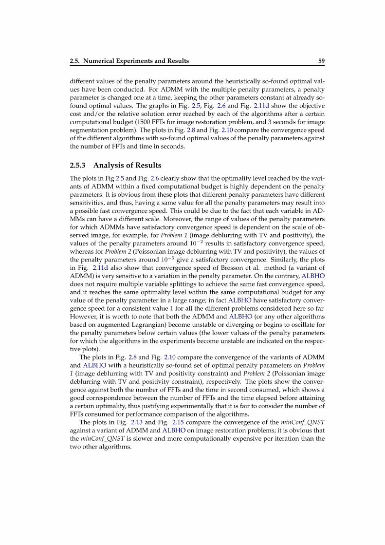
2.5. Numerical Experiments and Results 59
different values of the penalty parameters around the heuristically so-found optimal val-ues have been conducted. For ADMM with the multiple penalty parameters, a penaltyparameter is changed one at a time, keeping the other parameters constant at already so-found optimal values. The graphs in Fig. 2.5, Fig. 2.6 and Fig. 2.11d show the objectivecost and/or the relative solution error reached by each of the algorithms after a certaincomputational budget (1500 FFTs for image restoration problem, and 3 seconds for imagesegmentation problem). The plots in Fig. 2.8 and Fig. 2.10 compare the convergence speedof the different algorithms with so-found optimal values of the penalty parameters againstthe number of FFTs and time in seconds.
2.5.3 Analysis of Results
The plots in Fig.2.5 and Fig. 2.6 clearly show that the optimality level reached by the vari-ants of ADMM within a fixed computational budget is highly dependent on the penaltyparameters. It is obvious from these plots that different penalty parameters have differentsensitivities, and thus, having a same value for all the penalty parameters may result intoa possible fast convergence speed. This could be due to the fact that each variable in AD-MMs can have a different scale. Moreover, the range of values of the penalty parametersfor which ADMMs have satisfactory convergence speed is dependent on the scale of ob-served image, for example, for Problem 1 (image deblurring with TV and positivity), thevalues of the penalty parameters around 10−2 results in satisfactory convergence speed,whereas for Problem 2 (Poissonian image deblurring with TV and positivity), the values ofthe penalty parameters around 10−5 give a satisfactory convergence. Similarly, the plotsin Fig. 2.11d also show that convergence speed of Bresson et al. method (a variant ofADMM) is very sensitive to a variation in the penalty parameter. On the contrary, ALBHOdoes not require multiple variable splittings to achieve the same fast convergence speed,and it reaches the same optimality level within the same computational budget for anyvalue of the penalty parameter in a large range; in fact ALBHO have satisfactory conver-gence speed for a consistent value 1 for all the different problems considered here so far.However, it is worth to note that both the ADMM and ALBHO (or any other algorithmsbased on augmented Lagrangian) become unstable or diverging or begins to oscillate forthe penalty parameters below certain values (the lower values of the penalty parametersfor which the algorithms in the experiments become unstable are indicated on the respec-tive plots).
The plots in Fig. 2.8 and Fig. 2.10 compare the convergence of the variants of ADMMand ALBHO with a heuristically so-found set of optimal penalty parameters on Problem1 (image deblurring with TV and positivity constraint) and Problem 2 (Poissonian imagedeblurring with TV and positivity constraint), respectively. The plots show the conver-gence against both the number of FFTs and the time in second consumed, which shows agood correspondence between the number of FFTs and the time elapsed before attaininga certain optimality, thus justifying experimentally that it is fair to consider the number ofFFTs consumed for performance comparison of the algorithms.
The plots in Fig. 2.13 and Fig. 2.15 compare the convergence of the minConf_QNSTagainst a variant of ADMM and ALBHO on image restoration problems; it is obvious thatthe minConf_QNST is slower and more computationally expensive per iteration than thetwo other algorithms.

60 Chapter 2. A Nonsmooth Optimization Strategy for Inverse Problems in Imaging
ALBHO ADMM
Figure 2.3: Influence of penalty parameters on convergence: Comparison of ADMM andthe proposed ALBHO on a toy problem: x∗ := arg minx∈ΩxTQx+ bTx+ λ‖x‖1, whereQ ∈ R2×2 is a positive definite matrix, and x ∈ R2. The set Ω is the constrained region ingreen. The figure shows the contour plot of the objective function and the iterations of thetwo algorithms with a different penalty parameter, ρ. On the left is the plot of ALBHO, andon the right is ADMM. For small values of the penalty parameter, e.g., ρ = 0.1, both thealgorithms do not make any progress toward the minimum (get stuck), but for any otherlarger value, ALBHO always reaches the minimum, whereas ADMM converges only forvery particular values.
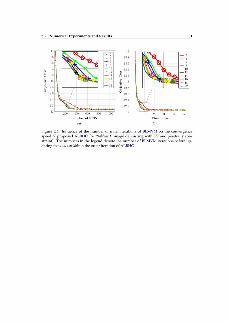
2.5. Numerical Experiments and Results 61
200 400 600 800 1,00012
12.2
12.4
12.6
12.8
13
13.2
13.4
13.6
13.8
14
number of FFTs
ObjectiveCost
2468101214161822
200 400 600 800 1,00012
12.2
12.4
12.6
12.8
13
13.2
13.4
13.6
13.8
14
number of FFTs
ObjectiveCost
2468101214161822
(a)
0 10 20 30 40 5012
12.2
12.4
12.6
12.8
13
13.2
13.4
13.6
13.8
14
Time in SecObjectiveCost
2468101214161822
0 10 20 30 40 5012
12.2
12.4
12.6
12.8
13
13.2
13.4
13.6
13.8
14
Time in Sec
ObjectiveCost
2468101214161822
(b)
Figure 2.4: Influence of the number of inner iterations of BLMVM on the convergencespeed of proposed ALBHO for Problem 1 (image deblurring with TV and positivity con-straint). The numbers in the legend denote the number of BLMVM iterations before up-dating the dual variable in the outer iteration of ALBHO.

62 Chapter 2. A Nonsmooth Optimization Strategy for Inverse Problems in Imaging
Osc
illa
tin
g/U
nst
able
regi
on
10−5 10−3 10−1 101 103 105 10712
13
14
15
16
17
18
Parameter: γ or ρ
ObjectiveCost
after1500FFTs
ADMM-3x (with fixed ρ, ν)ADMM-3x (with fixed ν, γ)
ADMM-1xALBHO
(a)
Osc
illa
ting/
Unst
able
regi
on
10−5 10−3 10−1 101 103 105 107−2 · 10−2
0
2 · 10−2
4 · 10−2
6 · 10−2
8 · 10−2
0.1
0.12
0.14
0.16
Parameter: γ or ρ(‖x
(150
0F
FT
s)−x∗ ‖
2)/‖x∗ ‖
2
ADMM-3x (with fixed ν, ρ)ADMM-3x (with fixed ν, γ)
ADMM-1xALBHO
(b)
Figure 2.5: Influence of augmented penalty parameters on convergence speed for differentalgorithms for Problem 1 (image deblurring with TV and positivity constraint). Penaltyparameters: Fixed ρ = 5 × 10⁻³, Fixed ν = 5 × 10⁻³, Fixed γ = 5 × 10⁻³, Regularizationparameter λ = 5× 10⁻⁴.
Osc
illa
ting/
Unst
able
regi
on
10−8 10−6 10−4 10−2 100 102 104
−5.17
−5.17
−5.17
−5.17
−5.17
−5.17
−5.17
·108
Parameter: γ or ρ
ObjectiveCost
after1500FFTs
ADMM-4x (fixed ρ, ν, η)ADMM-4x (fixed ν, γ, η)
ADMM-1xALBHO
(a)
Osc
illa
ting/
Unst
able
regi
on
10−8 10−6 10−4 10−2 100 102 104
0
2
4
6
8
·10−2
Parameter: γ or ρ
(‖x
(150
0F
FT
s)−
x∗ ‖
2)/‖x∗ ‖
2
ADMM-4x (fixed ρ, ν, η)ADMM-4x (fixex γ, ν, η )
ADMM1xALBHO
(b)
Figure 2.6: Influence of augmented penalty parameters on convergence speed of differentalgorithms for Problem 2 (Poissonian image deblurring with TV and positivity constraint).Penalty parameters: Fixed ρ = 5 × 10⁻⁶, Fixed ν = 5 × 10⁻⁶, Fixed η = 5 × 10⁻⁶, Fixedγ = 5× 10⁻⁶ Regularization parameter λ = 1× 10⁻³.
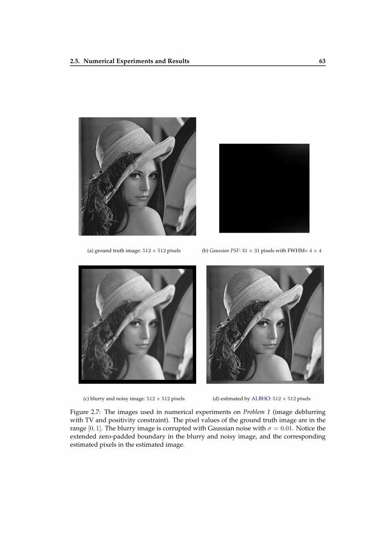
2.5. Numerical Experiments and Results 63
(a) ground truth image: 512× 512 pixels (b) Gaussian PSF: 31× 31 pixels with FWHM= 4× 4
(c) blurry and noisy image: 512× 512 pixels (d) estimated by ALBHO: 512× 512 pixels
Figure 2.7: The images used in numerical experiments on Problem 1 (image deblurringwith TV and positivity constraint). The pixel values of the ground truth image are in therange [0, 1]. The blurry image is corrupted with Gaussian noise with σ = 0.01. Notice theextended zero-padded boundary in the blurry and noisy image, and the correspondingestimated pixels in the estimated image.
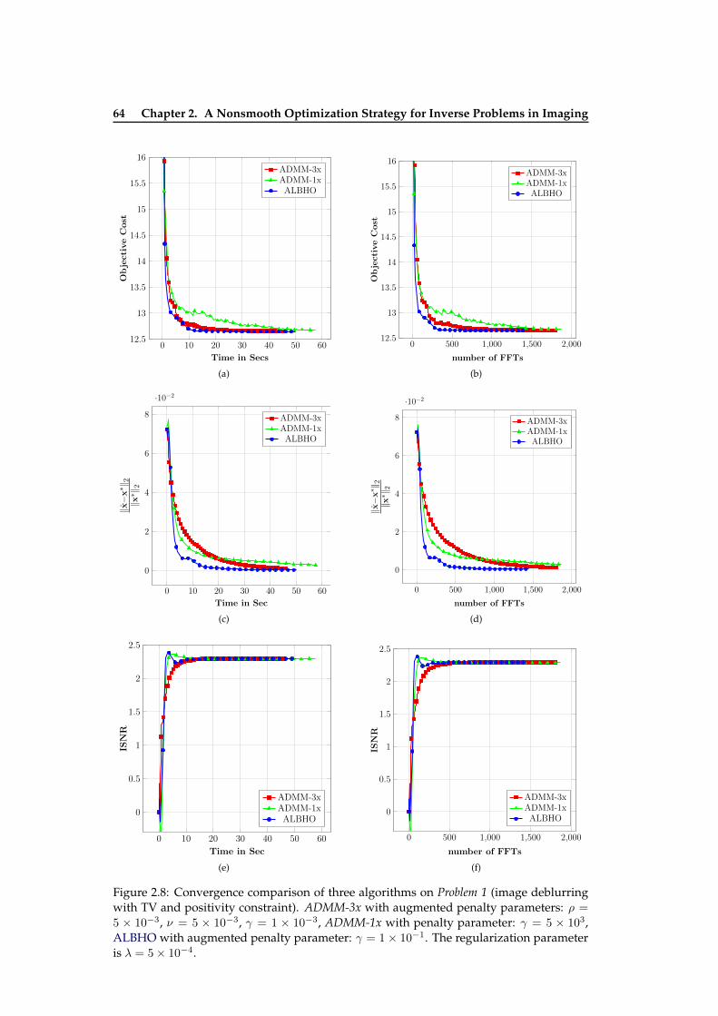
64 Chapter 2. A Nonsmooth Optimization Strategy for Inverse Problems in Imaging
0 10 20 30 40 50 6012.5
13
13.5
14
14.5
15
15.5
16
Time in Secs
ObjectiveCost
ADMM-3xADMM-1xALBHO
(a)
0 500 1,000 1,500 2,00012.5
13
13.5
14
14.5
15
15.5
16
number of FFTs
ObjectiveCost
ADMM-3xADMM-1xALBHO
(b)
0 10 20 30 40 50 60
0
2
4
6
8
·10−2
Time in Sec
‖x−x∗ ‖
2‖x∗ ‖
2
ADMM-3xADMM-1xALBHO
(c)
0 500 1,000 1,500 2,000
0
2
4
6
8
·10−2
number of FFTs
‖x−x∗ ‖
2‖x∗ ‖
2
ADMM-3xADMM-1xALBHO
(d)
0 10 20 30 40 50 60
0
0.5
1
1.5
2
2.5
Time in Sec
ISNR
ADMM-3xADMM-1xALBHO
(e)
0 500 1,000 1,500 2,000
0
0.5
1
1.5
2
2.5
number of FFTs
ISNR
ADMM-3xADMM-1xALBHO
(f)
Figure 2.8: Convergence comparison of three algorithms on Problem 1 (image deblurringwith TV and positivity constraint). ADMM-3x with augmented penalty parameters: ρ =
5 × 10⁻³, ν = 5 × 10⁻³, γ = 1 × 10⁻³, ADMM-1x with penalty parameter: γ = 5 × 10³,ALBHO with augmented penalty parameter: γ = 1× 10⁻¹. The regularization parameteris λ = 5× 10⁻⁴.
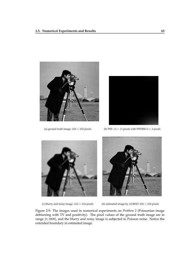
2.5. Numerical Experiments and Results 65
(a) ground truth image: 256× 256 pixels (b) PSF: 15× 15 pixels with FWHM=3× 3 pixels
(c) blurry and noisy image: 242× 242 pixels (d) estimated image by ALBHO: 256× 256 pixels
Figure 2.9: The images used in numerical experiments on Problem 2 (Poissonian imagedeblurring with TV and positivity). The pixel values of the ground truth image are inrange [0, 3000], and the blurry and noisy image is subjected to Poisson noise. Notice theextended boundary in estimated image.

66 Chapter 2. A Nonsmooth Optimization Strategy for Inverse Problems in Imaging
0 2 4 6 8 10 12 14−5.17
−5.17
−5.17
−5.17
−5.17
·108
Time in Sec
Objectiveco
st
ADMM-4x-AADMM-4x-BADMM-1xALBHO
0 2 4 6 8 10 12 14−5.17
−5.17
−5.17
−5.17
−5.17
·108
Time in Sec
Objectiveco
st
ADMM-4x-AADMM-4x-BADMM-1xALBHO
(a)
0 500 1,000 1,500 2,000 2,500−5.17
−5.17
−5.17
−5.17
−5.17
·108
number of FFTsObjectiveco
st
ADMM-4x-AADMM-4x-BADMM-1xALBHO
0 500 1,000 1,500 2,000 2,500−5.17
−5.17
−5.17
−5.17
−5.17
·108
number of FFTsObjectiveco
st
ADMM-4x-AADMM-4x-BADMM-1xALBHO
(b)
0 2 4 6 8 10 12 140
2 · 10−2
4 · 10−2
6 · 10−2
8 · 10−2
0.1
0.12
Time in Sec
(‖x−x∗ ‖
2)/‖x∗ ‖
2
ADMM-4x-AADMM-4x-BADMM-1xALBHO
0 2 4 6 8 10 12 140
2 · 10−2
4 · 10−2
6 · 10−2
8 · 10−2
0.1
0.12
Time in Sec
(‖x−
x∗ ‖
2)/‖x∗ ‖
2
ADMM-4x-AADMM-4x-BADMM-1xALBHO
(c)
0 500 1,000 1,500 2,000 2,500
0
2 · 10−2
4 · 10−2
6 · 10−2
8 · 10−2
0.1
0.12
number of FFTs
(‖x−x∗ ‖
2)/‖x∗ ‖
2
ADMM-4x-AADMM-4x-BADMM-1xALBHO
(d)
0 2 4 6 8 10 12 14−1
0
1
2
3
Time in Secs
ISNR
ADMM-4x-AADMM-4x-BADMM-1xALBHO
(e)
0 500 1,000 1,500 2,000 2,500−1
0
1
2
3
number of FFTs
ISNR
ADMM-4x-AADMM-4x-BADMM-1xALBHO
(f)
Figure 2.10: Convergence comparison of four algorithms on the Problem 2 (Poissonian im-age deblurring with TV and positivity). ADMM-4x with penalty parameters: ρ = 1×10⁻⁵,ν = 1 × 10⁻⁵, η = 1 × 10⁻⁵, γ = 5 × 10⁻⁶, ADMM-1x with augmented penalty param-eters: γ = 5 × 10⁻⁶, ALBHO with augmented penalty parameter: γ = 1 × 10⁻¹. Theregularization parameter: λ = 1× 10⁻³.
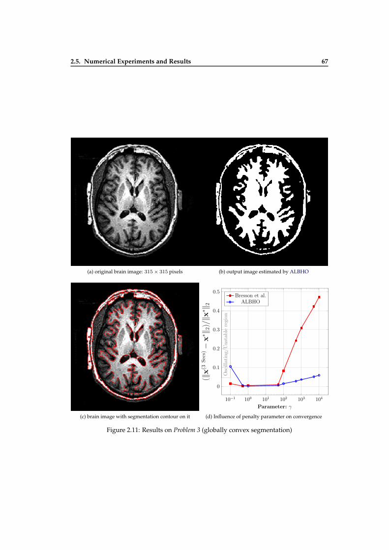
2.5. Numerical Experiments and Results 67
(a) original brain image: 315× 315 pixels (b) output image estimated by ALBHO
(c) brain image with segmentation contour on it
Oscillating/Unstab
leregion
10−1 100 101 102 103 104
0
0.1
0.2
0.3
0.4
0.5
Parameter: γ
(‖x(3
Secs)−x∗ ‖
2)/‖x∗ ‖
2
Bresson et al.ALBHO
(d) Influence of penalty parameter on convergence
Figure 2.11: Results on Problem 3 (globally convex segmentation)
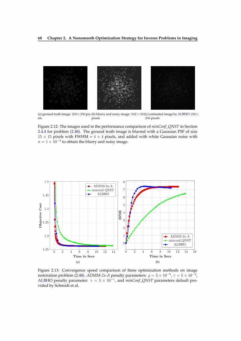
68 Chapter 2. A Nonsmooth Optimization Strategy for Inverse Problems in Imaging
(a) ground truth image: 256×256 pix-els
(b) blurry and noisy image: 242×242pixels
(c) estimated image by ALBHO: 256×256 pixels
Figure 2.12: The images used in the performance comparison of minConf_QNST in Section2.4.4 for problem (2.48). The ground truth image is blurred with a Gaussian PSF of size15 × 15 pixels with FWHM = 4 × 4 pixels, and added with white Gaussian noise withσ = 1× 10⁻³ to obtain the blurry and noisy image.
0 2 4 6 8 10 12 141.25
1.3
1.35
1.4
1.45
1.5
Time in Secs
ObjectiveCost
ADMM-2x-Aminconf QNST
ALBHO
(a)
0 2 4 6 8 10 12 14 16
0
1
2
3
4
5
6
7
8
Time in Secs
ISNR
ADMM-2x-Aminconf QNST
ALBHO
(b)
Figure 2.13: Convergence speed comparison of three optimization methods on imagerestoration problem (2.48). ADMM-2x-A penalty parameters: ρ = 5× 10⁻³, γ = 5× 10⁻²,ALBHO penalty parameter: γ = 5 × 10⁻¹, and minConf_QNST parameters default pro-vided by Schmidt et al.

2.5. Numerical Experiments and Results 69
(a) ground truth image: 256×256 pix-els
(b) blurry and noisy image: 256×256pixels
(c) estimated image by ALBHO: 256×256 pixels
Figure 2.14: The images used for the performance comparison of minConf_QNST in Section2.4.4 for problem (2.49). The observed image is obtained by blurring the true image with aGaussian PSF of size 15×15 pixels with FWHM = 4×4 pixels, and adding a white Gaussiannoise with σ = 5× 10⁻³.
0 2 4 6 8 10 12 14
2
3
4
5
6
7
8
9
10
Time in Secs
ObjectiveCost
ADMM-2x-Bminconf QNST
ALBHO
0 2 4 6 8 10 12 14
2
3
4
5
6
7
8
9
10
Time in Secs
ObjectiveCost
ADMM-2x-Bminconf QNST
ALBHO
(a)
0 2 4 6 8 10 12 14
−1.5
−1
−0.5
0
0.5
1
1.5
2
2.5
Time in Secs
ISNR
ADMM-2x(B)minconf QNST
ALBHO
(b)
Figure 2.15: Convergence speed comparison of three optimization methods. ADMM-2x-Bpenalty parameters: ρ = 5× 10⁻², γ = 5× 10⁻², ALBHO penalty parameter: γ = 5× 10⁻²,and minConf_QNST default parameters provided by Schmidt et al.
70 Chapter 2. A Nonsmooth Optimization Strategy for Inverse Problems in Imaging
2.6 Conclusions
• Large-scale constrained convex nonsmooth optimization problems arise in many ap-plications in signal/image processing, computer vision, and machine learning.
• Proximal forward-backward iterative methods are state-of-the-art methods for solv-ing these types of optimization problem.
• In the last two decades, ADMM, which also belongs to proximal forward-backwarditerative method, has evolved as a prominent optimization strategy for large-scaleconvex optimization problem.
• Variants of ADMM have been shown to be faster than all other algorithms in proxi-mal forward-backward iterative schemes provided that
– it introduces enough variable splittings such that each subproblem has a closed-form solution,
– each augmented penalty parameter associated with augmented term is tunedoptimally.
• Optimal tuning of augmented penalty parameters is still an open challenge.
• The convergence speed of ADMM is highly dependent on the values of the aug-mented penalty parameters.
• In this thesis, I proposed an optimization algorithm named ALBHO for large-scalenonsmooth constrained convex optimization problems, which is as fast as the fastestvariant of ADMM.
• ALBHO avoids multiple variable splittings, and it is almost parameter tuning free(its convergence speed is almost insensitive to the augmented penalty parameter).
• ALBHO uses a limited-memory quasi-Newton method with bound constraint, thus,it directly handles the bound constraints without any extra effort (variable splitting)unlike the ADMM.
• I illustrated the applicability and performance of ALBHO on different inverse prob-lems in imaging and computer vision, which proves that ALBHO is a viable alterna-tive method for optimization problems in signal/image processing, computer visionand machine learning.
2.7 Summary
This chapter is entirely devoted to numerical optimization techniques suitable for im-age restoration problem. It discusses different existing optimization approaches for con-strained nonsmooth optimization problems, and then proposes a new class of optimizationalgorithms based on augmented Lagrangian and hierarchical optimization strategy. Theproposed algorithm is as efficient as the state-of-art algorithms with an advantage overthem that it is almost parameter tuning free.
CHAPTER 3
Image Decomposition Approachfor Image Restoration
What has been already divided into parts cannot be recovered backfrom them without adding to the total entropy.
– Anonymous
Contents3.1 Introduction . . . . . . . . . . . . . . . . . . . . . . . . . . . . . . . . . . . . . . 723.2 Signal Decomposition Approaches . . . . . . . . . . . . . . . . . . . . . . . . . 733.3 An Approach Toward Astronomical Image Restoration via Image Decompo-
sition and Blind Image Deblurring . . . . . . . . . . . . . . . . . . . . . . . . . 763.3.1 Introduction . . . . . . . . . . . . . . . . . . . . . . . . . . . . . . . . . 763.3.2 The Objective and The Proposed Approach . . . . . . . . . . . . . . . 773.3.3 The Likelihood and The Priors . . . . . . . . . . . . . . . . . . . . . . . 783.3.4 Blind Image Deblurring as a Constrained Minimization Problem . . . 803.3.5 Selection of Hyperparameters . . . . . . . . . . . . . . . . . . . . . . . 823.3.6 Experiments and Results . . . . . . . . . . . . . . . . . . . . . . . . . . 833.3.7 Analysis of Results . . . . . . . . . . . . . . . . . . . . . . . . . . . . . 83
3.4 Conclusion and Perspective . . . . . . . . . . . . . . . . . . . . . . . . . . . . . 973.5 Summary . . . . . . . . . . . . . . . . . . . . . . . . . . . . . . . . . . . . . . . 98
72 Chapter 3. Image Decomposition Approach for Image Restoration
Abstract
Signal decomposition is a very fundamental approach in many signal processing appli-cations. The classic and still pervasive example is Fourier analysis which breaks peri-odical signals into sinusoidal (smooth oscillating) components. In the last two decades,image decomposition into fundamental components or more semantic components hasbeen proven to be a very effective tool for several image processing/computer vision ap-plications such as image restoration, image segmentation, image compression, image en-cryption, etc. This chapter starts with a general overview of image decomposition and itsapplication in image processing problems, specifically in image restoration (denoising anddeblurring). A major part of this chapter is dedicated to an approach toward astronom-ical image restoration via image decomposition and blind image deblurring. The resultsof the proposed blind image restoration on synthetically blurred and noisy astronomicalimages are promising; it suggests that such an approach can be used in real scenarios aftercertain modifications and improvements in its ingredients, such as the noise model, andthe priors.
3.1 Introduction
A very basic approach in signal processing is to decompose an original signal into itsprimitive or fundamental constituents and to perform simple operations separately oneach component, thereby accomplishing extremely sophisticated operations by a combi-nation of individually simple operations. The typical assumption for such an approachin many applications is that the given signal is a linear mixture of several source signalsof a more coherent origin. The classical and still pervasive example is Fourier analysis[Fourier 1808], the theory and practice that breaks signals into sinusoidal (smooth oscil-lating) components, e.g., a complex sound can be decomposed into rich combinationsof simple tones. The Fourier methods have been supplemented by other approaches,most notably the many methods now subsumed under the general heading of wavelets[Mallat 1993, Kahane 1995, Mallat 1999]. These alternatives hold promise for providingmore useful ways of analyzing and processing signals for different applications. Thesedecompositions have been a key to theoretical tools for the modern communications tech-niques e.g., understanding and advancement of error-control coding (finite field wavelettransform for design of multiresolution analysis for multilevel error-control coding) andcompression for reliable communications, signal processing for removing unwanted noiseand signals, and for improving the quality of signals.
Another trend is the decomposition of a given signal into more semantic componentsrather than into fundamental constituents using Fourier transform or simple wavelets.This decomposition is commonly referred to as source separation. A classical example isthe cocktail party problem where a sound signal containing several concurrent speaker isto be separated into the sound emanating from each speaker. In image processing, a simi-lar situation is encountered in many cases, e.g., photographs containing transparent layersdue to reflection. During recent years, this decomposition trend has evolved as a viabletool in image restoration problem, e.g., decomposition of a natural image into geometricaland textural components, decomposition of an astronomical image into point-like sources(stars) and extended smooth sources (comets, galaxies). Since image restoration problemsare often ill-posed, they need appropriate regularizations, from a Bayesian point-of-view,the image decomposition into more appropriate and adapted domains can be seen as pro-viding more informative prior to them.
3.2. Signal Decomposition Approaches 73
Both signal decomposition trends, the decomposition into fundamental constituentsand the decomposition into more semantic components have been shown to be very use-ful in image restoration applications. However, image restorations using the first decom-position trend have been mostly used for problems like signal denoising, where the effortis on discrimination of the random noise from the meaningful signal, whereas the seconddecomposition trend is used in applications where the extraction of different semanticcomponents is beneficial, e.g., restoring only cartoon and textural parts precisely whilemitigating the noise in image deblurring problems. Similarly, extracting precisely the con-tours/edges in a degraded image improves the accuracy of PSF estimation in blind imagedeblurring process. In the coming sections, we will see some applications of the secondtrend of image decomposition relevant to image restoration problems.
3.2 Signal Decomposition Approaches
The existing signal decomposition approaches in the literature can be coarsely catego-rized into two groups: synthesis-based approach, and analysis-based approach (the au-thors in [Elad 2007] present a detailed comparison between these two approaches andalso show under what conditions these two approaches are similar or differ from eachother). The synthesis-based approach uses a sparse representation of a signal into sets ofatoms, commonly referred to as dictionaries of functions, and matching pursuit schemes(e.g. stagewise orthogonal matching pursuit and morphological component analysis)to achieve the decomposition [Zibulevsky 2001, Starck 2005a, Fadili 2010]. The analysis-based approach uses different functional space norms and partial differential equationsmethods to achieve the decomposition, commonly referred to as variational formulation[Vese 2003, Osher 2003, Aujol 2005a, Aujol 2006]. There also exist some image decompo-sition techniques, e.g. [Starck 2005b, Aujol 2005b], which merge these approaches to takeadvantages of both and obtain better results.Synthesis Based Approach: Zibulevsky’s seminal work [Zibulevsky 2001] initiated thesparsity based approaches for source separation. The success of such an approach is basedon two principles: sparsity and morphological diversity, i.e. each semantic component issparsely representable in a specific dictionary (transformed domain), and this dictionaryis highly non-sparse in representing the other components of the mixture. A dictionaryis consist of atoms, which are elementary signals representing templates, e.g., sinusoids,monomials, wavelets, Gaussians, etc. A dictionary Φ = [ϕ1, · · · ,ϕm] defines a n × m
matrix whose columns are unit l2-norm atoms ϕk. A dictionary is called overcomplete orredundant when m > n = rank(Φ). A common assumption is that a signal or an imagex ∈ Rn is the linear superposition of K components, possibly contaminated with noise:
x =
K∑k=1
xk + ε, σ2ε = Var[ε] < +∞ (3.1)
A popular source separation approach based on sparsity and morphological diversity ispresented in [Starck 2005a]. It assumes that each component xk is sparsely representablein an associated basis Φk:
xk = Φkαk, k = 1, · · · ,K, (3.2)
where αk is a sparse coefficient vector. Thus, a dictionary can be built by assemblingseveral transforms (Φ1, · · · ,ΦK) such that, for each k, the representation of xk in Φk issparse and non-sparse in other Φl, l 6= k, then the source separation is done by solving the

74 Chapter 3. Image Decomposition Approach for Image Restoration
following underdetermined system of equations:
α1, · · · ,αK := arg minα1,··· ,αK
K∑k=1
‖αk‖pp such that ‖y −K∑k=1
Φkαk‖2 ≤ τ (3.3)
where the most interesting regime is 0 ≤ p ≤ 1 for sparsity, and τ is typically chosen asa constant times
√nσε. The problem (3.3) is a hard problem, especially when p < 1 (for
p = 0 it is even NP-hard). Nevertheless, if all the components xl = Φlαl but the k-thare fixed, then it is shown in [Starck 2005a] that solution αk is given by hard-thresholding(for p = 0) or soft-thresholding (for p = 1) the marginal residual rk = y −∑l 6=k Φlαl inthe transformed domain. The algorithm presented in [Starck 2005a] is basically a block-coordinate relaxation algorithm (or alternating minimization method) that cycles throughthe components at each iteration and applies a thresholding to the marginal residuals inthe transformed domain.
The success of such an approach is very much dependent on the choice of the dictionar-ies for the components to be separated. Of course there are no perfect dictionaries allowinga sparse representation of all the features/structures in an image, however it has been ob-served that most of the isotropic structures can be coded efficiently by wavelets presentedin [Mallat 1999]. The curvelet system [Candès 2006] is a good candidate for representingpiecewise smooth features in images. Similarly, the ridgelet transform [Candes 1999] hasbeen shown to be effective for representing global lines in an image. For locally oscillatingtextures, local DCTs (discrete cosine transform) [Mallat 1993], Waveatoms [Demanet 2007],Brushlets [Meyer 1997] are proven to be effective. These transforms are computationallytractable for large-scale problems, and they do not require to be built explicitly. The as-sociated implicit fast analysis and synthesis operators have typical complexities of orderO(n) (e.g., orthogonal or bi-orthogonal wavelets transforms) or O(n log n) (e.g., ridgelets,curvelets, local DCTs, and Waveatoms). When no fixed a priori dictionary is able to rep-resent faithfully and sparsely a certain components (e.g. a complex natural texture), theauthors in [Peyre 2007] have shown that a more effective and adaptive dictionary can belearned from a set of exemplars.Analysis Based Approach: The approach is based on the assumption that a certain compo-nent of a signal is well captured in a certain functional space, i.e., a semantic componentof a signal has a smaller norm in a certain functional space than in any other functionalspace. This assumption makes it possible to do signal decomposition by energy minimiza-tion techniques. The seminal paper of Rudin-Osher-Fatemi (ROF) [Rudin 1992] introducednonlinear partial differential equation methods in image processing problems. The ROFmodel is based on the assumption that discontinuities along curves in images, commonlycalled geometrical or cartoon parts, belong to Bounded-Variation Banach space BV(Ω),which is the subspace of functions x ∈ L1(Ω) such that their total variation, TV(x) is fi-nite. The total variation of x is defined as: TV(x) = |Dx|(Ω), which is a distributionalderivative on the domain of image, Ω, an open connected set of R2 with Lipschitz bound-ary1. If x has gradient ∇x ∈ L1(Ω), then TV(x) =
∫Ω|∇x(u)| du, where |t| =
√t21 + t22
for all t ∈ R2. The ROF model has been shown very effective for the preservation of thesharp features (edges) in images while suppressing the fine textural details. The imagedecomposition into a component x belonging to BV and a component z in L2 based on
1A Lipschitz domain (or domain with Lipschitz boundary) is a domain in Euclidean space whose boundaryis “sufficiently regular” in the sense that it can be thought of as locally being the graph of a Lipschitz continuousfunction.

3.2. Signal Decomposition Approaches 75
TV -L2 model is achieved by the following energy minimization:
arg minx∈BV
TV(x) +
1
2λ‖y − x‖22
(3.4)
where y ∈ X is the image to be decomposed, and the latter component is given by z = y−x. This model performs well for denoising images while preserving the edges, however,fine details, such as textures, are suppressed. Meyer introduced a space G in [Meyer 2001]for oscillating patterns, e.g., textures. G is the Banach space composed of the distributionsz = ∂1g1 + ∂2g2 = div(g), with g1 and g2 in L∞(Ω). The space G is endowed with thefollowing norm:
‖z‖G = inf‖g‖L∞(Ω;R2) : z = div(g)
with ‖g‖L∞(Ω,R2) = supu∈Ω
√‖g1‖2 + ‖g2‖2(u). This space happens to be very close to the
dual space2 of BV. In this space the oscillating patterns have a small norm, thus the normon G is well-adapted to capture the oscillations of a function in an energy minimizationmethod. The image decomposition into components x belonging to BV and z belongingto G, proposed by Meyer in [Meyer 2001], also referred as TV -G model, is achieved by thefollowing energy minimization:
arg minx∈BV
TV(x) +
1
2λ‖y − x‖G
(3.5)
where the latter component is given by z = y − x. Meyer also suggested another spaceE to capture oscillating patterns. The space E is defined as G, but now the g1, g2 belongsto Besov space B∞−1,∞(Ω) 3. The image decomposition into x belonging to BV , and zbelonging to E, also referred as TV -E model, is achieved by the following energy mini-mization:
arg minx∈BV
TV(x) +
1
λ‖y − x‖E
(3.6)
where the latter component is given by z = y − x. Meyer did not provide any numericalscheme in [Meyer 2001] to solve the above minimization problems (3.5) and (3.6), and thesolutions to these problems are quite difficult to compute due to the complexity of theG and E norms. The solutions to model (3.5) (or quite close problems) are proposed in[Vese 2003, Aujol 2003, Aujol 2005a].
In Appendix, A.2, we will see some applications (e.g., denoising, deblurring) of theabove image decomposition models. In the next Section 3.3, I present an approach forastronomical image restoration via an image decomposition model and blind image de-blurring. The image decomposition model used in the image restoration problem is ananalysis-based approach, where the image is decomposed into two semantic maps by us-ing sparsity inducing prior and smoothness inducing as well as an edges preserving prior.
2A linear form on a vector space V is f : V → R satisfying f(u + v) = f(u) + f(v), and f(cu) =cf(u),where u ∈ V,v ∈ V, c ∈ R. The dual space V ∗ is the collection of all linear forms. If V is finite dimensionalthen V ∗ has the same dimension as V . The dual norm of f is defined as ‖f‖∗ = sup|f(u)| : u ∈ V, ‖u‖2 ≤ 1.
3The dual space of E = B∞−1,∞ is B11,1. B1
1,1 is the usual Besov space. Let ψj,k represent the orthonormalbase composed of smooth and compactly supported wavelets. B1
1,1 is a subspace of L2(R2), and function f
belongs to B11,1 if and only if:
∑j∈Z
∑k∈Z2 |cj,k| < +∞, where cj,k are the wavelet coefficients of f .
76 Chapter 3. Image Decomposition Approach for Image Restoration
3.3 An Approach Toward Astronomical Image Restorationvia Image Decomposition and Blind Image Deblurring
Remark: The work presented in this section was accepted at 23rd EUSIPCO 2015, Nice,under the title "A Blind Deblurring and Image Decomposition Approach For AstronomicalImage Restoration" [Mourya 2015a], and received the “Best Student Paper Award”.
3.3.1 Introduction
Acquiring photometrically precise and high resolution images from a ground-based imag-ing system is highly desirable and remains a long-standing problem in astronomy. The at-mospheric turbulence is the major culprit for the distortions in the acquired images. Withthe progress of adaptive optics (AO) systems [Davies 2012], the PSFs of ground-based tele-scopes have been brought closer to the diffraction limit and the resolution of the acquiredimages has improved drastically. However, the compensation for atmospheric turbulenceis still partial [Conan 2000, Rigaut 2000, Drummond 2009]. This leaves good scope fordigital restoration techniques to recover fine details in the images, which are very impor-tant for the astrophysical interpretations. Considering the uncertainty in the measurement(calibration) of PSF and variability of long-exposure PSF with time, blind image deblur-ring (BID) has been shown [Ayers 1988, Molina 2001, Mugnier 2004] to be a viable imagerestoration technique for restoring the fine details in those images.
Image restoration, in general, has a long history that began in the 1950s with astro-nomical image restoration, however, the development of blind image deblurring can betraced back to the 1970s [Cannon 1976]; see [Molina 2001] for a survey on astronomicalimage restoration. Blind image deblurring has been vastly explored for restoring natu-ral images degraded by motion blur and camera defocus, see [Almeida 2010, Levin 2011a]and the references within, but relatively few articles are available on works dedicatedto astronomical image restoration; [Cannon 1976, Lane 1992, Molina 1992, Jefferies 1993,Tsumuraya 1994, Schulz 1997, Thiébaut 1995, Conan 2000, Thiébaut 2002, Mugnier 2004,Chao 2006, Harmeling 2009] are the prominent ones to be mentioned. The blind imagedeblurring approaches are specific to the applications, however, most of these successfulapproaches are built on a Bayesian framework differing primarily by the stage at which thePSF is estimated, and what priors are included about the image and/or the PSF. Accord-ing to the stage at which the PSF is estimated in these methods, they can be categorizedinto two groups: a priori blur identification methods, and simultaneous blur identifica-tion methods. In the first category, the PSF is identified separately from the blurred andnoisy image and then it is used by a non-blind deblurring method to get the crisp image.For example, an experimental approach for astronomical images is to collect one or morepoint sources in the image, and then use them to obtain an estimate of the PSF. An anothersophisticated approach in this category is due to [Likas 2004, Molina 2006, Levin 2011a],in which the PSF is estimated a priori by marginalizing over a high-dimensional space ofimage using variational Bayesian strategy. In the second category, both the unknowns (theunderlying PSF and the image) are estimated simultaneously, mostly using an alternat-ing minimization approach [Ayers 1988, Chan 2000] in which the underlying PSF and theimage are estimated in alternating steps, rather than by a truly joint minimization. Themajority of techniques found in the literature fall into the second category due to threemain reasons: i). a priori estimated PSF may not be always very accurate for certain tech-nical reasons, ii). marginalization involved in the approach by Levin et al. [Levin 2011a]cannot be evaluated in straightforward way considering real image prior, and thus it in-
3.3. An Approach Toward Astronomical Image Restoration via Image Decompositionand Blind Image Deblurring 77
volves many unjustified approximations [Wipf 2014], and iii). the alternating estimationapproaches are easier to understand, implement, and are computationally less expensivecompared to marginalization approach. Another advantage of alternating estimation ap-proach is that the approximate a priori estimate of the PSF, either by experimental methodsor by model fitting methods, can always serve as a good initial guess of PSF to start the al-ternating estimation, and with progress of the alternation one can ensure a better estimateof the underlying PSF and the image by imposing appropriate priors on both the PSF andthe image.
3.3.2 The Objective and The Proposed Approach
Considering that the compensation of the effect of atmospheric turbulence provided bythe adaptive optics system is partial, in this work I put an effort in the enhancement of thequality of the images captured under an adaptive optics system by a blind image deblur-ring approach. The proposed approach for astronomical image restoration is an instanceof maximum-a-posteriori estimation, and the unknowns are estimated by alternating min-imization. The proposed approach for blind image deblurring considers an appropriatenoise model, an image prior via image decomposition, and necessary prior on the PSF.From now onward, I will refer to the proposed approach by the name “Blind Deblur-ring via Image Decomposition” (BDID). Here in this work, BDID is only applicable to therestoration of the narrow field-of-view images, nevertheless, it can be used for wide field-of-view images after certain modifications (this is the subject of discussion in Chapter 4).Before we proceed toward the details of the BDID, I will recall here the image formationmodel and restate the blind image deblurring problem.
For a narrow field of view, the PSF of an imaging system can be considered stationary,and the blurred and noisy image y formed at the focal plane of the imaging system due tothe underlying sharp image x can be modeled by the discretized image formation model:
y = P(H x) + n (3.7)
where n is a vector drawn from a white Gaussian distribution, P denotes a Poisson ran-dom process,H is the discrete convolution matrix corresponding to the PSF h. The imageformation model (3.7) is valid once the scale of image values is expressed in photons, andthe background and the flat field corrections have been done on the raw blurry and noisyimage. Blind image deconvolution is stated as the estimation of both the underlying PSF,h, and the crisp image, x, given only the observed blurred and noisy image y.
As discussed in Chapter 1, blind image deblurring is an ill-posed inverse problem,thus, appropriate priors on both the unknowns, x and h are necessary to regularize (re-strict) the solution to be meaningful. The maximum-a-posteriori (MAP) estimation:
x∗,h∗MAP = arg maxx,h
p(y|x,h)p(x)p(h) (3.8)
is one of the well known approaches for blind image deblurring, which considers estimat-ing the unknown quantities jointly. The first term, p(y|x,h), in above formulation (3.8),commonly referred to as likelihood, is dependent on the noise statistics and image forma-tion model, and the remaining two terms, p(x) and p(h), are prior on the image and thePSF, respectively, that impose any prior knowledge on the sought quantities. The aboveformulation of blind image deblurring can be equivalently casted as the following mini-mization problem:
x∗,h∗MAP = arg minx,h
− log p(y|x,h)− log p(x)− log p(h) (3.9)

78 Chapter 3. Image Decomposition Approach for Image Restoration
By looking at the above formulation of blind image deconvolution, it is obvious that thetwo important ingredients of blind image deblurring are: i). the problem specific noisemodel and the priors on the PSF and the image, and ii). the optimization algorithm, whichmust be efficient enough to reach the solution within a reasonable computational budget.
Contribution: As discussed in previous sections, certain dictionaries in the synthesis-based approach or certain functional spaces in analysis-based approach, are able to wellrepresent or capture the semantic components in images, thus image decomposition mod-els have been shown to be effective for image restoration in several works [Osher 2003,Giovannelli 2005, Daubechies 2005, Starck 2005b, Wang 2015]. From a Bayesian point ofview, this can be seen as providing better priors for each semantic component in the imagethat we want to restore. Many astronomical images can be described as a superimpositionof two types of components: point-like sources (PS) and extended smooth sources (ES), ona dark background. Recovering precisely the position and intensity of PS embedded in ESis of great interest for astronomers, and PS are very effective features in the astronomicalimages for precisely estimating the unknown PSF. In this work, the image decompositionapproach of [Giovannelli 2005] is adopted and extended to a blind image deblurring set-ting. Since the two components are very different from each other, obviously two differentpriors are suitable for each of them. PS are sparse in the spatial domain, thus a spatialsparsity promoting prior is imposed on the unknown image for extracting the PS map.ES are often piecewise smoothness, thus a smoothness inducing edge preserving prior isimposed on the unknown image for the extraction of the ES map. An appropriate prioron the PSF is imposed as well relevant to adaptive optics system. A noise model, whichis simple yet very efficient to represent a mixture of white Gaussian and Poisson noise,is considered. The resulting optimization problem is solved by alternating minimization,in which each subproblem is solved efficiently by BLMVM proposed in Chapter 2. Thedetails of each ingredient of the BDID is presented in what follows.
3.3.3 The Likelihood and The Priors
Likelihood: The noise present in astronomical images can be fairly represented by a mix-ture of white Gaussian and Poisson noise, as expressed in image formation model (3.7).Thus, the non-stationary white Gaussian noise model (also referred as Weighted LeastSquare (WL2) ) presented in [Mugnier 2004] is adopted in this work. This noise model isa pretty accurate approximation for a mixture of Gaussian and Poisson noise while keep-ing the complexity arising in the optimization problem at a moderate level. We believethat sufficiently accurate and simple noise model with strict a priori on the solution canresult into better behavior of the blind image deconvolution than a more complex noisemodel, which can hinder in strict enforcement of the constraints. Recently, the authors in[Chouzenoux 2015] show that an exact Poisson-Gaussian likelihood for mixture of Pois-son and white Gaussian noise can result into better image quality than the WL2 model oncertain example images considered by them, but at the cost of increasing the complexityof the resulting optimization problem.
Dropping out the constant terms and the terms independent of x and h, the likelihoodterm for non-stationary white Gaussian noise can be written approximately as:
− log p(y|x,h) =∑i
1
2 σ2i
(y − h ∗ x)2i =
1
2‖y −Hx‖2W (3.10)
where (σi)2 = (σphi )2 + (σdeti )2, and (σphi )2 and (σdeti )2 are the photon and the detector noise
variances at the ith pixel, respectively. W is a diagonal and inverse of noise covariance
3.3. An Approach Toward Astronomical Image Restoration via Image Decompositionand Blind Image Deblurring 79
matrix, i.e., W i,j = δi,j/σ2i , where δi,j represents Kronecker delta. The quantities σph and
σdet can be estimated from the blurred and noisy image as suggested in [Mugnier 2004],and also discussed in Chapter 1 Section 1.7. For unknown measurements, such as dead orsaturated or boundary pixels,W i,i = 0, is considered, as also suggested in [Matakos 2013]for correctly handling boundaries.
Image Priors: From a statistical point of view, the PS can be modeled as sparse uncorre-lated pixels, thus, a sparsity inducing `1-norm is imposed on the image for PS. The ES aresmoothly varying correlated pixels may be with some sharp edges, thus a smoothness in-ducing edge-preserving prior, such as total variation, can be imposed. But, as mentionedpreviously, total variation preserves well only the sharp edges and suppresses the subtledetails, thus, an intermediate behavior prior, such as Huber-function (a hybrid `1/`2-norm)on gradient image is more appropriate for the ES, since, in many cases ES is not only piece-wise smooth, but may also contain some fine textures. In this way, using two priors, twoseparate maps: xP and xE , are estimated from the single blurry and noisy image, thencombined together to get the final estimate of the underlying image. An important physi-cal constraint, such as the positivity of these maps, is also imposed. Now, the prior on PSand ES are written as:
− log p(xP ) = λ‖xP ‖1, xP ≥ 0 (3.11)
− log p(xE) = µ∑i
φδ(Di xE), xE ≥ 0 (3.12)
where
φδ(t) =
12‖t‖22 ‖t‖2 6 δ
δ(‖t‖2 − δ2 ) ‖t‖2 > δ
is the Huber-function, D = [DT(1),D
T(2)]
T represents two dimensional finite first-orderdifference operator, and Di x ∈ R2 represents the gradient vector at the ith pixel ofthe image. λ, µ > 0 are tunable hyperparameters, and δ ≥ 0 is a threshold. TheHuber-function on gradient image is an intermediate between total variation and squared`2-norm of the gradient image, and its behavior is adjusted by δ. It is worth to mentionthat the staircase artifact produced by total variation can be avoided in Huber-norm byadjusting the threshold.
PSF Prior: For ground-based large telescopes, there are mainly two regimes of imaging:long and short (less than≈ 1/4 second) exposures. Short exposure images take the form ofspeckle patterns, consisting of multiple distorted and overlayed copies of the diffraction-limited PSF. In order to increase the signal-to-noise ratio, almost all astronomical imagingis performed with long exposures, unless conditions (such as high sky brightness in theinfrared) prevent it. Because the short-exposure PSFs are highly variable, both in structureand centroid position, the summed long-exposure PSF is highly blurred compared to thediffraction-limit, even with good seeing conditions. Thanks to the real-time correction ofthe AO system, the long-exposure PSF is maintained closer to the diffraction-limit, but be-cause of some remaining perturbations in the imaging system, the effective PSF still hassome uncorrected parts. Several measurements of PSF done at Gemini north and Keckobservatory [Drummond 2009] reveal that the uncorrected part of the PSF are approxi-mately Lorentzian or Gaussian shape or both atop the Airy pattern. The PSF of the AOcorrected imaging system is quite smooth with small aberrations, thus a smoothness in-ducing squared `2-norm on gradient of the sought PSF is chosen as a prior for the PSF.The PSF of the considered imaging system is always positive and upper bounded by the

80 Chapter 3. Image Decomposition Approach for Image Restoration
peak value of the diffraction-limited PSF. Moreover, the blurring process is considered tofollow energy conservation, i.e., the total intensity of the blurry image is equal to the totalintensity of the underlying crisp image, thus a normalization constraint on the PSF is verynecessary. With all these constraints the prior on PSF is written as:
− log p(h) =η
2
∑i
‖Dih‖22, 0 ≤ h ≤ α, 1Th = 1. (3.13)
where α is the peak value of the Airy pattern for a given aperture, and η > 0 is a hyperpa-rameter.
3.3.4 Blind Image Deblurring as a Constrained Minimization Problem
Substituting all the analytical expressions of the terms in (3.9), blind image deblurring isexpressed as a constrained optimization problem:
x∗P ,x∗E ,h∗MAP = arg minxP ,xE ,h
1
2‖y −H(xP + xE)‖2W + λ‖xP ‖1 + µ
∑i
φδ(DixE)
+η
2
∑i
‖Dih‖22
such that xP ≥ 0, xE ≥ 0, 0 ≤ h ≤ α, 1Th = 1. (3.14)
This is a difficult large-scale nonsmooth nonconvex optimization. It still may have severallocal minima even though we restrict its solution space with all the possible penalties andconstraints. Few authors [Lane 1992, Thiébaut 2002] take a joint minimization approach(estimating simultaneously x and h) to solve the optimization problem arising in blindimage deconvolution, and [Thiébaut 2002] considers the several issues arising in joint min-imization, but their optimization problems are comparatively simpler in the sense that thepriors used are simple. In the optimization problem (3.14), it is easy to realize that theproblem is convex with respect to one of the unknown variables when considering theother fixed, thus, a much simpler and widespread approach is to perform Alternating Min-imization, as presented in Algorithm BDID on page 81. One can reach a good expectedlocal minimum by Algorithm BDID, provided that one starts with a good initial guess ofthe PSF. Luckily, in the case of astronomical imaging, finding a good initial guess of thePSF is not always a tedious task; one could extract it from the blurry and noisy image itselfby selecting a few blurry point-like sources (reference stars), otherwise one could ask forcalibrated PSF from the astronomers (they always have model fitted PSF to characterizetheir imaging system). The calibrated PSF of an imaging system with AO is quite close tothe true PSF, and can serve as a good initial guess.
The optimization problems (3.15) and (3.16) in BDID are solved by the variable split-ting trick, and transforming the resulting constrained optimization problem into an un-constrained problem by forming the augmented Lagrangian. The solution is then foundby ALBHO proposed in Chapter 2. With the variables splittings: zP = xP and zE = ∇xE ,the augmented Lagrangian of the problem (3.15) is written as:
Lρ1,ρ2(xP ,xE , zP , zE ,uP ,uE) =1
2‖y −H(xP + xE)‖2W + ιC(xP ) + λ‖zP ‖1
+ρ1
2‖xP − zP + uP ‖22 + ιC(xE) +
∑i
µφδ(zE)i +ρ2
2‖(∇xE − zE + uE)i‖22
(3.17)
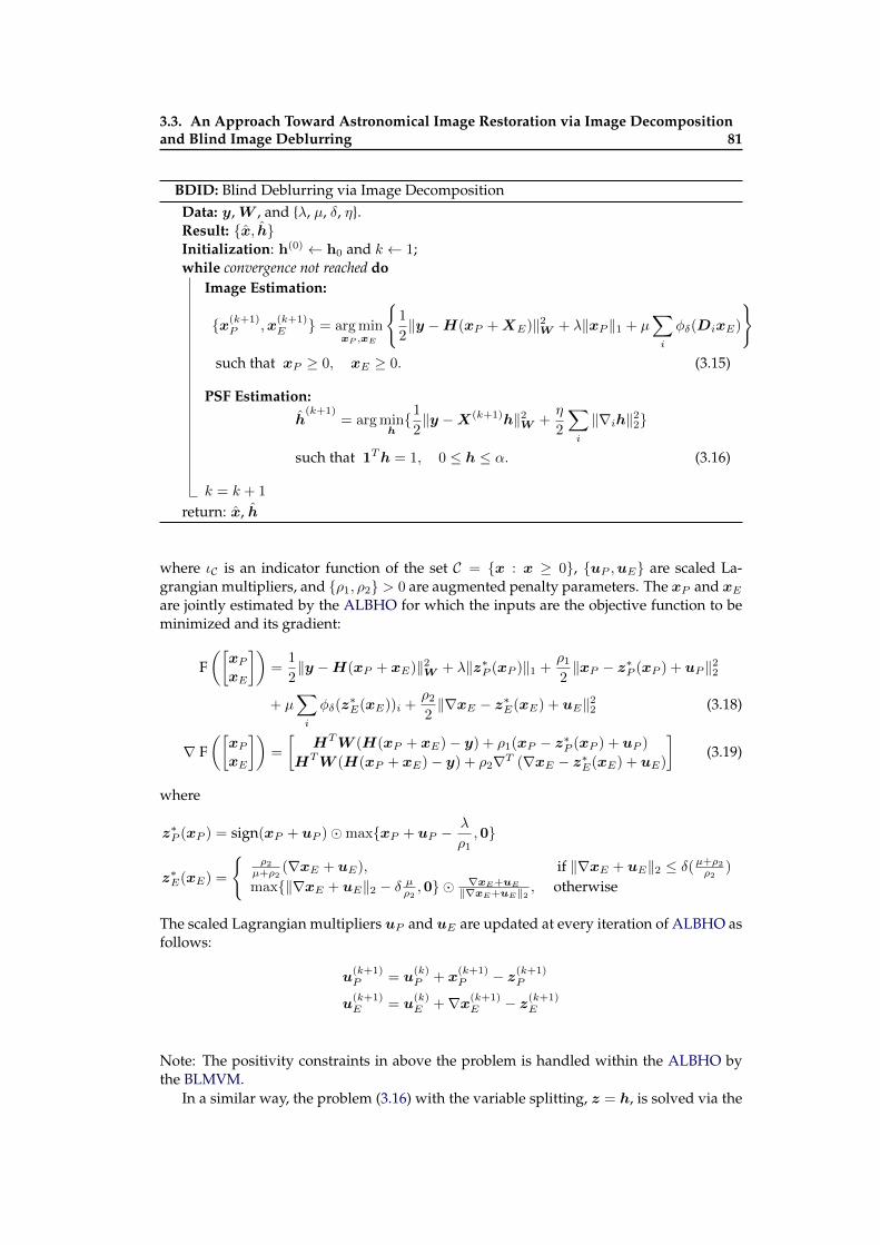
3.3. An Approach Toward Astronomical Image Restoration via Image Decompositionand Blind Image Deblurring 81
BDID: Blind Deblurring via Image DecompositionData: y,W , and λ, µ, δ, η.Result: x, hInitialization: h(0) ← h0 and k ← 1;while convergence not reached do
Image Estimation:
x(k+1)P ,x
(k+1)E = arg min
xP ,xE
1
2‖y −H(xP +XE)‖2W + λ‖xP ‖1 + µ
∑i
φδ(DixE)
such that xP ≥ 0, xE ≥ 0. (3.15)
PSF Estimation:
h(k+1)
= arg minh1
2‖y −X(k+1)h‖2W +
η
2
∑i
‖∇ih‖22
such that 1Th = 1, 0 ≤ h ≤ α. (3.16)
k = k + 1
return: x, h
where ιC is an indicator function of the set C = x : x ≥ 0, uP ,uE are scaled La-grangian multipliers, and ρ1, ρ2 > 0 are augmented penalty parameters. The xP and xEare jointly estimated by the ALBHO for which the inputs are the objective function to beminimized and its gradient:
F([xPxE
])=
1
2‖y −H(xP + xE)‖2W + λ‖z∗P (xP )‖1 +
ρ1
2‖xP − z∗P (xP ) + uP ‖22
+ µ∑i
φδ(z∗E(xE))i +
ρ2
2‖∇xE − z∗E(xE) + uE‖22 (3.18)
∇ F([xPxE
])=
[HTW (H(xP + xE)− y) + ρ1(xP − z∗P (xP ) + uP )
HTW (H(xP + xE)− y) + ρ2∇T (∇xE − z∗E(xE) + uE)
](3.19)
where
z∗P (xP ) = sign(xP + uP )maxxP + uP −λ
ρ1,0
z∗E(xE) =
ρ2
µ+ρ2(∇xE + uE), if ‖∇xE + uE‖2 ≤ δ(µ+ρ2
ρ2)
max‖∇xE + uE‖2 − δ µρ2 ,0 ∇xE+uE‖∇xE+uE‖2 , otherwise
The scaled Lagrangian multipliers uP and uE are updated at every iteration of ALBHO asfollows:
u(k+1)P = u
(k)P + x
(k+1)P − z(k+1)
P
u(k+1)E = u
(k)E +∇x(k+1)
E − z(k+1)E
Note: The positivity constraints in above the problem is handled within the ALBHO bythe BLMVM.
In a similar way, the problem (3.16) with the variable splitting, z = h, is solved via the
82 Chapter 3. Image Decomposition Approach for Image Restoration
augmented Lagrangian:
Lρ3(h, z,u) =1
2‖y −Xh‖2W +
η
2
∑i
‖∇ih‖22 + ιΘ(z) +ρ3
2‖h− z + u‖22 (3.20)
where X is the discrete convolution matrix corresponding to the image x, and ιΘ(t) is anindicator function that t belongs to a probability simplex: Θ = t : t ≥ 0,1T t = 1. Theρ3 > 0 is an augmented penalty parameter, and u is a scaled Lagrange multiplier. Onceagain, the problem (3.20) is solved by the ALBHO for which the inputs are the objectivefunction and its gradient:
F(h) =1
2‖y −Xh‖2W +
η
2
∑i
‖∇ih‖22 +ρ3
2‖h− z∗(h) + u‖22 (3.21)
∇ F(h) = XTW (Xh− y) + η∇T∇h+ ρ3(h− z∗(h) + u) (3.22)
where
z∗(h) = ΠΘ(h+ u) (3.23)
The projection, ΠΘ, onto the simplex of Rn can be computed by the O(n log n) algorithmproposed in [Wang 2013].
As illustrated in Chapter 2, the choices of the augmented penalty parameters are notcritical, since the ALBHO is almost parameter tuning free. The iterations of the ALBHOfor each subproblem in BDID can be stopped once it reaches a certain maximum numberor attains a certain optimality condition as described in Chapter 2. It is not necessary tosolve each of the subproblems in BDID very accurately for the BDID to reach the expectedgood local minimum. In fact, in experiments, I found that the BDID behaves better whenthe accuracy is increased gradually with every iteration of the BDID. This is due to the factthat the initial PSF is not close to the actual PSF, thus it is not necessary to estimate theimage up to very high accuracy with this initial PSF, and gradually when the estimationof PSF gets better, one can progressively increase the accuracy of image estimation. Inmy implementation, this is achieved by progressively increasing the number of iterationstaken by ALBHO at every iteration of BDID. The outer iterations in BDID are stopped oncethe relative change in the estimated image reaches a certain small value.
3.3.5 Selection of Hyperparameters
The BDID includes three tunable hyperparameters, λ, µ, η ≥ 0, and a tunable threshold,δ ≥ 0. The hyperparameters balance the likelihood term and the priors, and their valuesare related to noise variance in the blurry and noisy image. Hyperparameter λ controlsthe sparsity in the PS map, µ and δ control the smoothness and sharp edges in the ES map,and the η controls the smoothness of the PSF. A good balance among the hyperparametersis essential to obtain a satisfactory decomposition into PS and ES maps. However, find-ing optimal values for the hyperparameters is a non-trivial task, but at the same time itmakes the BDID flexible. If one believes that the blurry and noisy image contains only PS,then one can mask out the ES setting µ → ∞ (and conversely λ → ∞ to suppress pointsources). In the numerical experiments, the hyperparameters were chosen after a few tri-als to achieve the highest peak signal-to-noise ratio, PSNR= 10 log10
(max(xref ))2
‖xref−x‖22, where x
and xref are the estimated and the reference images, respectively.
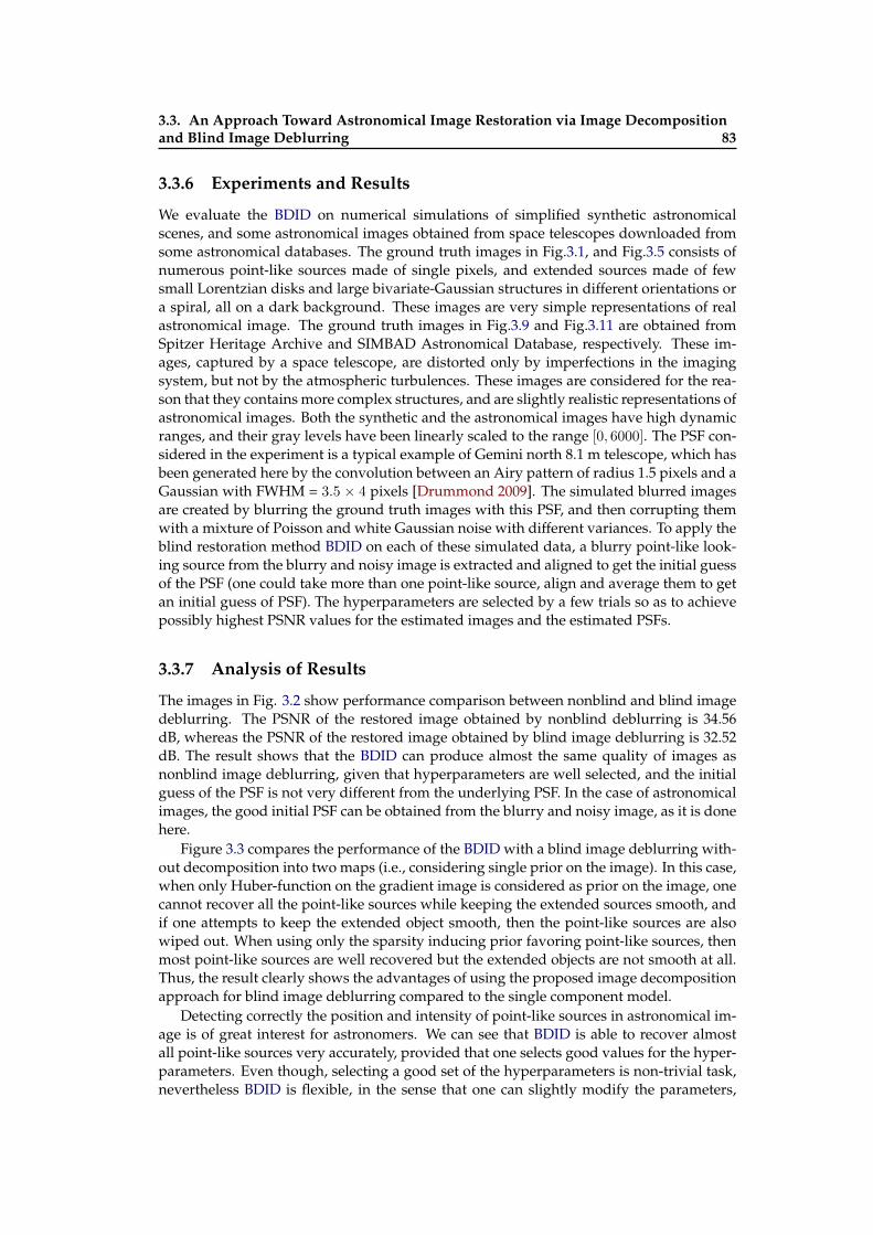
3.3. An Approach Toward Astronomical Image Restoration via Image Decompositionand Blind Image Deblurring 83
3.3.6 Experiments and Results
We evaluate the BDID on numerical simulations of simplified synthetic astronomicalscenes, and some astronomical images obtained from space telescopes downloaded fromsome astronomical databases. The ground truth images in Fig.3.1, and Fig.3.5 consists ofnumerous point-like sources made of single pixels, and extended sources made of fewsmall Lorentzian disks and large bivariate-Gaussian structures in different orientations ora spiral, all on a dark background. These images are very simple representations of realastronomical image. The ground truth images in Fig.3.9 and Fig.3.11 are obtained fromSpitzer Heritage Archive and SIMBAD Astronomical Database, respectively. These im-ages, captured by a space telescope, are distorted only by imperfections in the imagingsystem, but not by the atmospheric turbulences. These images are considered for the rea-son that they contains more complex structures, and are slightly realistic representations ofastronomical images. Both the synthetic and the astronomical images have high dynamicranges, and their gray levels have been linearly scaled to the range [0, 6000]. The PSF con-sidered in the experiment is a typical example of Gemini north 8.1 m telescope, which hasbeen generated here by the convolution between an Airy pattern of radius 1.5 pixels and aGaussian with FWHM = 3.5 × 4 pixels [Drummond 2009]. The simulated blurred imagesare created by blurring the ground truth images with this PSF, and then corrupting themwith a mixture of Poisson and white Gaussian noise with different variances. To apply theblind restoration method BDID on each of these simulated data, a blurry point-like look-ing source from the blurry and noisy image is extracted and aligned to get the initial guessof the PSF (one could take more than one point-like source, align and average them to getan initial guess of PSF). The hyperparameters are selected by a few trials so as to achievepossibly highest PSNR values for the estimated images and the estimated PSFs.
3.3.7 Analysis of Results
The images in Fig. 3.2 show performance comparison between nonblind and blind imagedeblurring. The PSNR of the restored image obtained by nonblind deblurring is 34.56dB, whereas the PSNR of the restored image obtained by blind image deblurring is 32.52dB. The result shows that the BDID can produce almost the same quality of images asnonblind image deblurring, given that hyperparameters are well selected, and the initialguess of the PSF is not very different from the underlying PSF. In the case of astronomicalimages, the good initial PSF can be obtained from the blurry and noisy image, as it is donehere.
Figure 3.3 compares the performance of the BDID with a blind image deblurring with-out decomposition into two maps (i.e., considering single prior on the image). In this case,when only Huber-function on the gradient image is considered as prior on the image, onecannot recover all the point-like sources while keeping the extended sources smooth, andif one attempts to keep the extended object smooth, then the point-like sources are alsowiped out. When using only the sparsity inducing prior favoring point-like sources, thenmost point-like sources are well recovered but the extended objects are not smooth at all.Thus, the result clearly shows the advantages of using the proposed image decompositionapproach for blind image deblurring compared to the single component model.
Detecting correctly the position and intensity of point-like sources in astronomical im-age is of great interest for astronomers. We can see that BDID is able to recover almostall point-like sources very accurately, provided that one selects good values for the hyper-parameters. Even though, selecting a good set of the hyperparameters is non-trivial task,nevertheless BDID is flexible, in the sense that one can slightly modify the parameters,
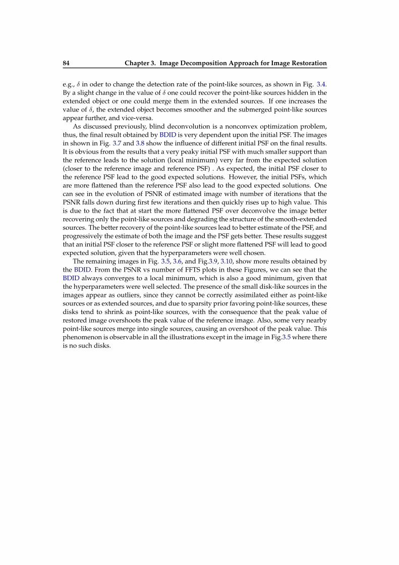
84 Chapter 3. Image Decomposition Approach for Image Restoration
e.g., δ in oder to change the detection rate of the point-like sources, as shown in Fig. 3.4.By a slight change in the value of δ one could recover the point-like sources hidden in theextended object or one could merge them in the extended sources. If one increases thevalue of δ, the extended object becomes smoother and the submerged point-like sourcesappear further, and vice-versa.
As discussed previously, blind deconvolution is a nonconvex optimization problem,thus, the final result obtained by BDID is very dependent upon the initial PSF. The imagesin shown in Fig. 3.7 and 3.8 show the influence of different initial PSF on the final results.It is obvious from the results that a very peaky initial PSF with much smaller support thanthe reference leads to the solution (local minimum) very far from the expected solution(closer to the reference image and reference PSF) . As expected, the initial PSF closer tothe reference PSF lead to the good expected solutions. However, the initial PSFs, whichare more flattened than the reference PSF also lead to the good expected solutions. Onecan see in the evolution of PSNR of estimated image with number of iterations that thePSNR falls down during first few iterations and then quickly rises up to high value. Thisis due to the fact that at start the more flattened PSF over deconvolve the image betterrecovering only the point-like sources and degrading the structure of the smooth-extendedsources. The better recovery of the point-like sources lead to better estimate of the PSF, andprogressively the estimate of both the image and the PSF gets better. These results suggestthat an initial PSF closer to the reference PSF or slight more flattened PSF will lead to goodexpected solution, given that the hyperparameters were well chosen.
The remaining images in Fig. 3.5, 3.6, and Fig.3.9, 3.10, show more results obtained bythe BDID. From the PSNR vs number of FFTS plots in these Figures, we can see that theBDID always converges to a local minimum, which is also a good minimum, given thatthe hyperparameters were well selected. The presence of the small disk-like sources in theimages appear as outliers, since they cannot be correctly assimilated either as point-likesources or as extended sources, and due to sparsity prior favoring point-like sources, thesedisks tend to shrink as point-like sources, with the consequence that the peak value ofrestored image overshoots the peak value of the reference image. Also, some very nearbypoint-like sources merge into single sources, causing an overshoot of the peak value. Thisphenomenon is observable in all the illustrations except in the image in Fig.3.5 where thereis no such disks.
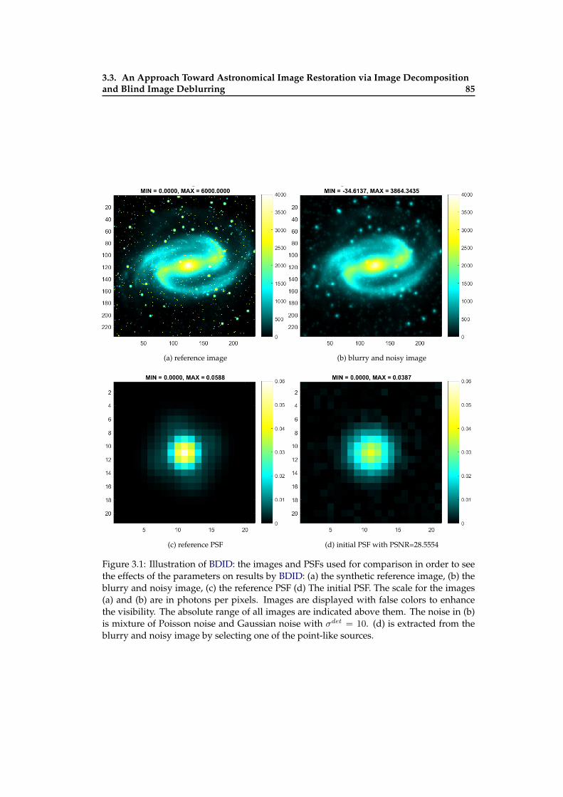
3.3. An Approach Toward Astronomical Image Restoration via Image Decompositionand Blind Image Deblurring 85
(a) reference image (b) blurry and noisy image
(c) reference PSF (d) initial PSF with PSNR=28.5554
Figure 3.1: Illustration of BDID: the images and PSFs used for comparison in order to seethe effects of the parameters on results by BDID: (a) the synthetic reference image, (b) theblurry and noisy image, (c) the reference PSF (d) The initial PSF. The scale for the images(a) and (b) are in photons per pixels. Images are displayed with false colors to enhancethe visibility. The absolute range of all images are indicated above them. The noise in (b)is mixture of Poisson noise and Gaussian noise with σdet = 10. (d) is extracted from theblurry and noisy image by selecting one of the point-like sources.
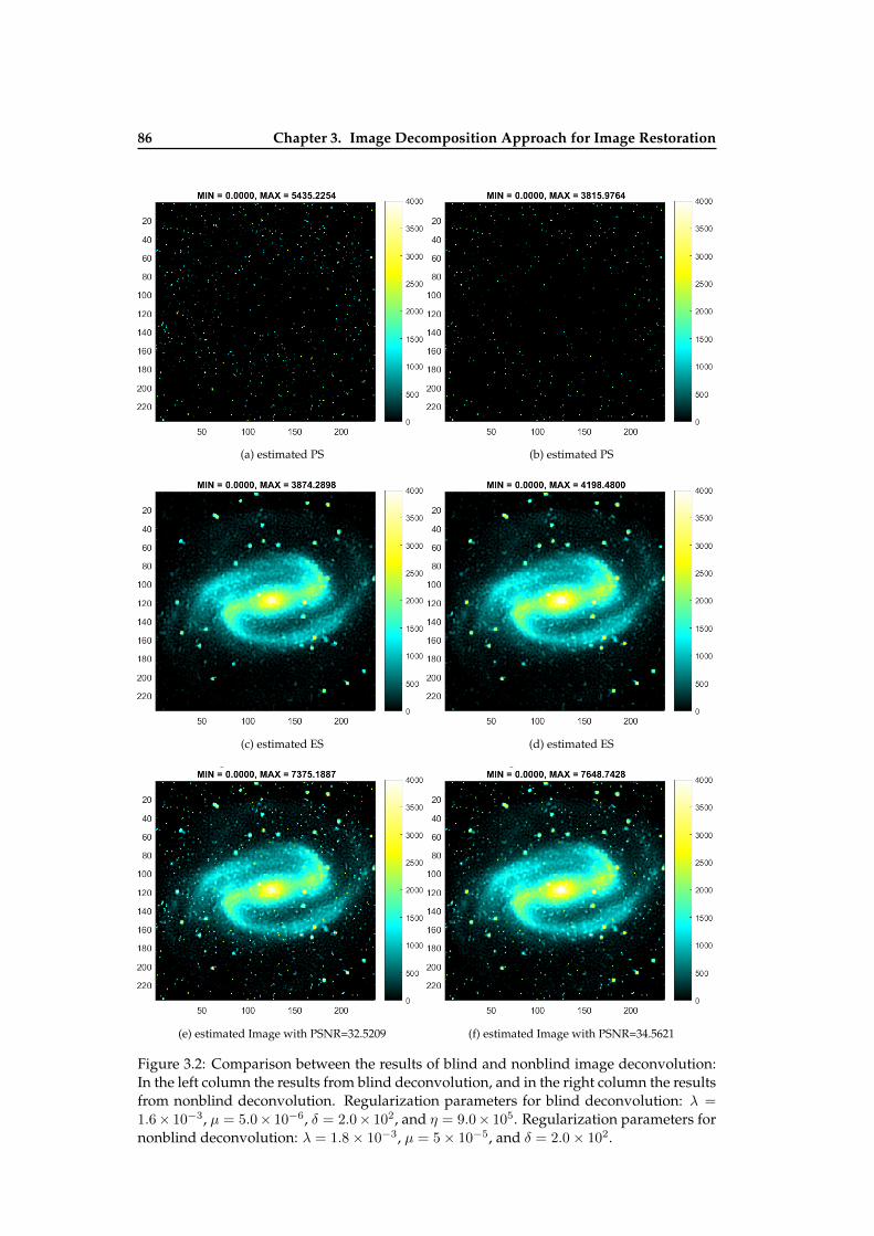
86 Chapter 3. Image Decomposition Approach for Image Restoration
(a) estimated PS (b) estimated PS
(c) estimated ES (d) estimated ES
(e) estimated Image with PSNR=32.5209 (f) estimated Image with PSNR=34.5621
Figure 3.2: Comparison between the results of blind and nonblind image deconvolution:In the left column the results from blind deconvolution, and in the right column the resultsfrom nonblind deconvolution. Regularization parameters for blind deconvolution: λ =
1.6× 10⁻³, µ = 5.0× 10⁻⁶, δ = 2.0× 10², and η = 9.0× 10⁵. Regularization parameters fornonblind deconvolution: λ = 1.8× 10⁻³, µ = 5× 10⁻⁵, and δ = 2.0× 10².
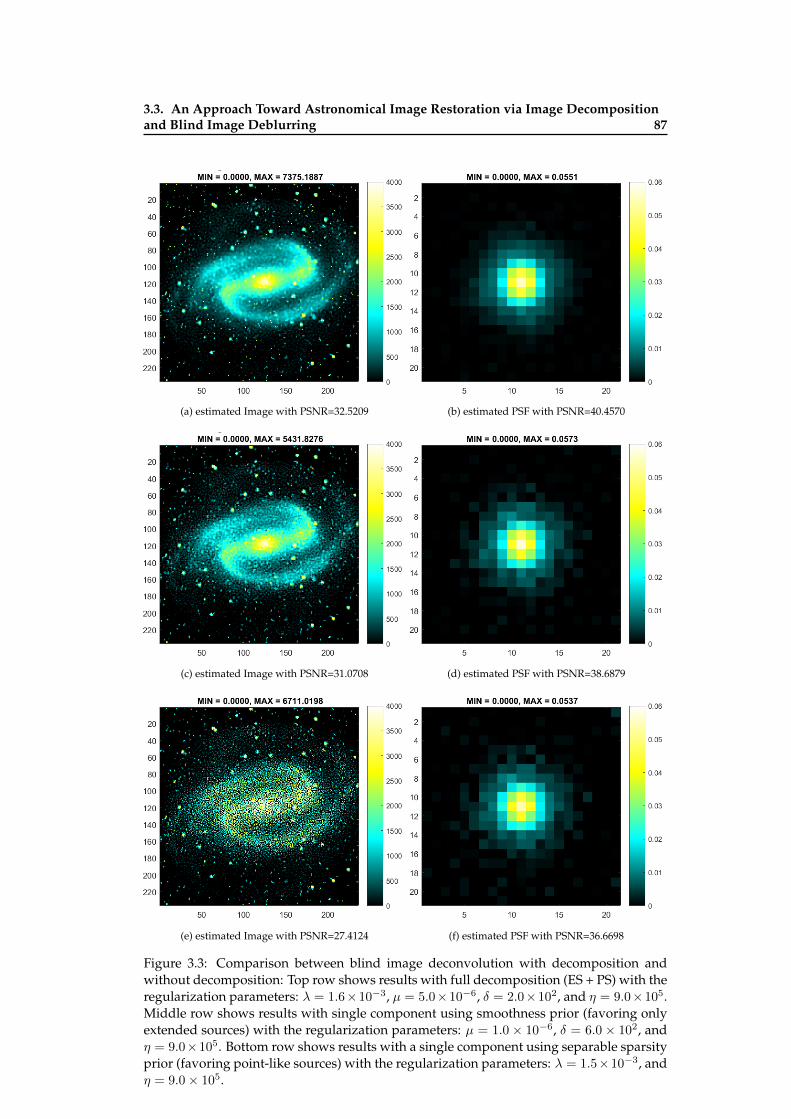
3.3. An Approach Toward Astronomical Image Restoration via Image Decompositionand Blind Image Deblurring 87
(a) estimated Image with PSNR=32.5209 (b) estimated PSF with PSNR=40.4570
(c) estimated Image with PSNR=31.0708 (d) estimated PSF with PSNR=38.6879
(e) estimated Image with PSNR=27.4124 (f) estimated PSF with PSNR=36.6698
Figure 3.3: Comparison between blind image deconvolution with decomposition andwithout decomposition: Top row shows results with full decomposition (ES + PS) with theregularization parameters: λ = 1.6×10⁻³, µ = 5.0×10⁻⁶, δ = 2.0×10², and η = 9.0×10⁵.Middle row shows results with single component using smoothness prior (favoring onlyextended sources) with the regularization parameters: µ = 1.0 × 10⁻⁶, δ = 6.0 × 10², andη = 9.0×10⁵. Bottom row shows results with a single component using separable sparsityprior (favoring point-like sources) with the regularization parameters: λ = 1.5×10⁻³, andη = 9.0× 10⁵.
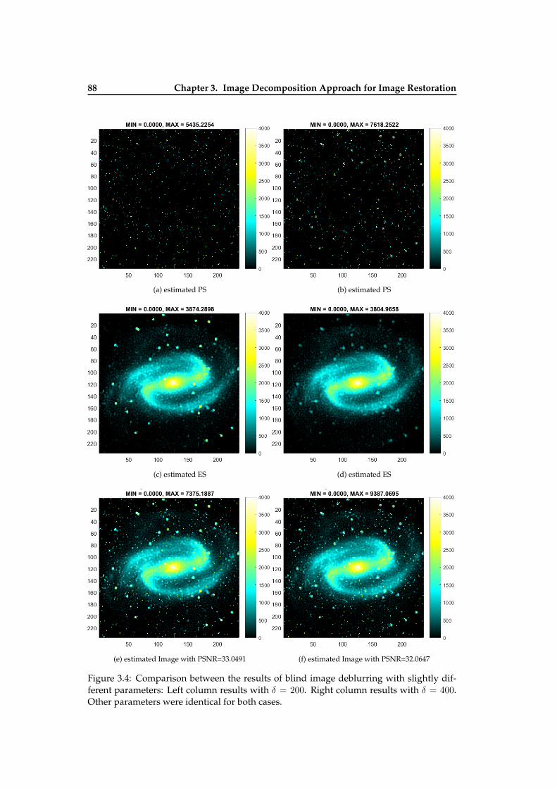
88 Chapter 3. Image Decomposition Approach for Image Restoration
(a) estimated PS (b) estimated PS
(c) estimated ES (d) estimated ES
(e) estimated Image with PSNR=33.0491 (f) estimated Image with PSNR=32.0647
Figure 3.4: Comparison between the results of blind image deblurring with slightly dif-ferent parameters: Left column results with δ = 200. Right column results with δ = 400.Other parameters were identical for both cases.
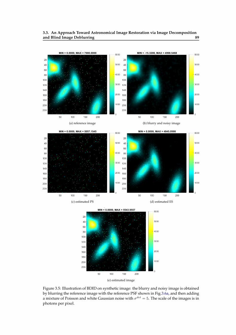
3.3. An Approach Toward Astronomical Image Restoration via Image Decompositionand Blind Image Deblurring 89
(a) reference image (b) blurry and noisy image
(c) estimated PS (d) estimated ES
(e) estimated image
Figure 3.5: Illustration of BDID on synthetic image: the blurry and noisy image is obtainedby blurring the reference image with the reference PSF shown in Fig.3.6a, and then addinga mixture of Poisson and white Gaussian noise with σdet = 5. The scale of the images is inphotons per pixel.
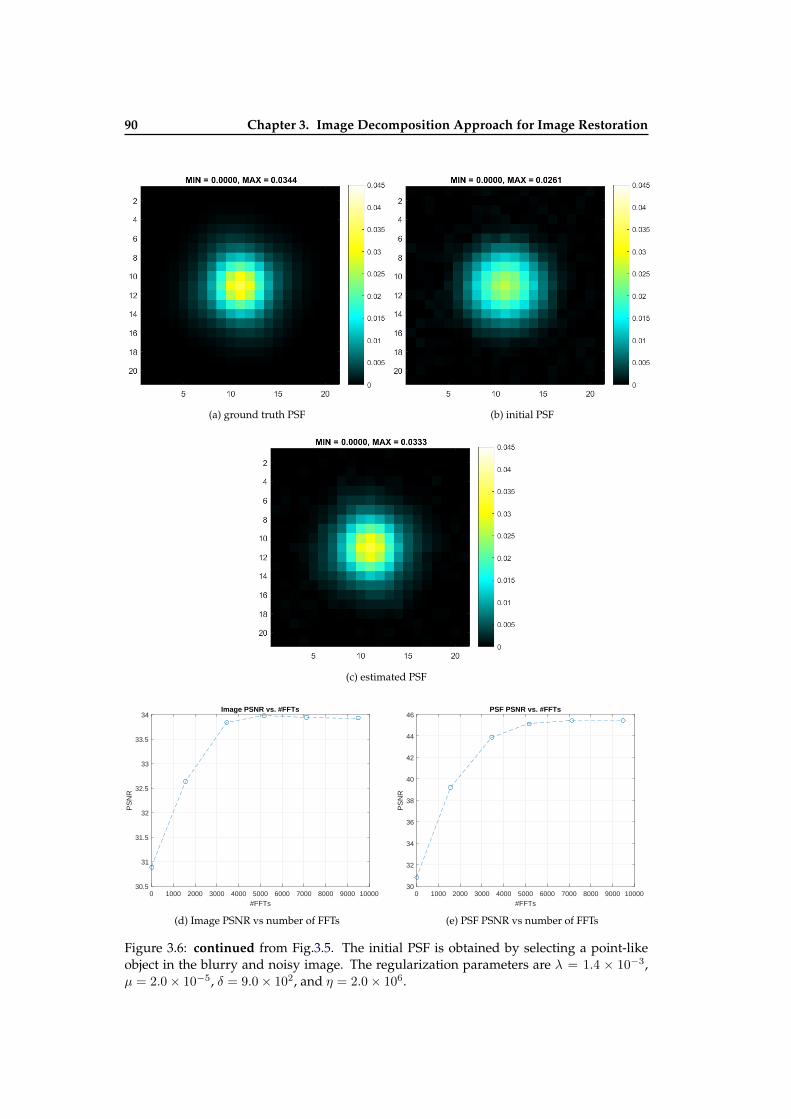
90 Chapter 3. Image Decomposition Approach for Image Restoration
(a) ground truth PSF (b) initial PSF
(c) estimated PSF
0 1000 2000 3000 4000 5000 6000 7000 8000 9000 10000
#FFTs
30.5
31
31.5
32
32.5
33
33.5
34
PS
NR
Image PSNR vs. #FFTs
(d) Image PSNR vs number of FFTs
0 1000 2000 3000 4000 5000 6000 7000 8000 9000 10000
#FFTs
30
32
34
36
38
40
42
44
46
PS
NR
PSF PSNR vs. #FFTs
(e) PSF PSNR vs number of FFTs
Figure 3.6: continued from Fig.3.5. The initial PSF is obtained by selecting a point-likeobject in the blurry and noisy image. The regularization parameters are λ = 1.4 × 10⁻³,µ = 2.0× 10⁻⁵, δ = 9.0× 10², and η = 2.0× 10⁶.
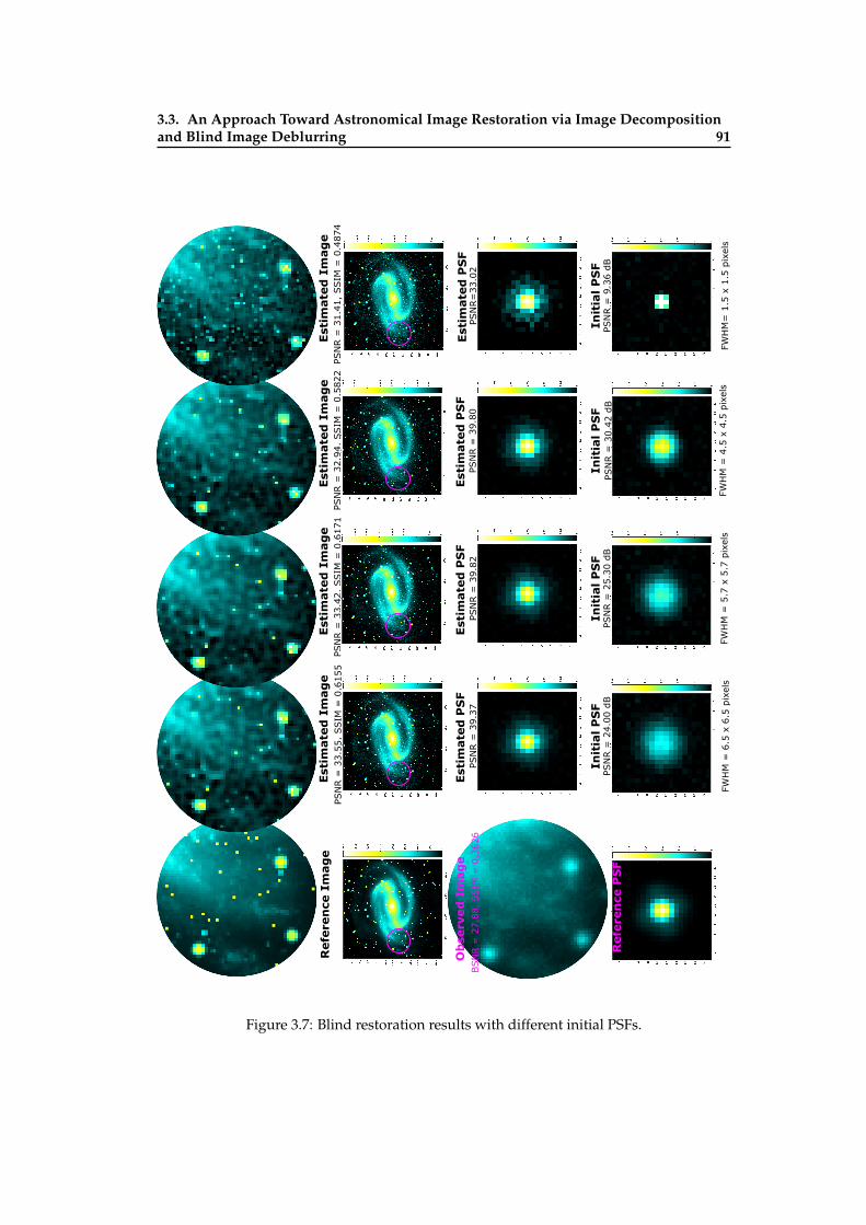
3.3. An Approach Toward Astronomical Image Restoration via Image Decompositionand Blind Image Deblurring 91
PSN
R =
30.4
2 d
BPS
NR =
25.3
0 d
BPS
NR =
9.3
6 d
BIn
itia
l P
SF
PSN
R =
24.0
0 d
B
FWH
M =
6.5
x 6
.5 p
ixel
sFW
HM
= 5
.7 x
5.7
pix
els
FWH
M =
4.5
x 4
.5 p
ixel
sFW
HM
= 1
.5 x
1.5
pix
els
Init
ial
PS
FIn
itia
l P
SF
Init
ial
PS
F
PSN
R=
33.0
2PS
NR =
39.8
0PS
NR =
39.8
2PS
NR =
39.3
7
PSN
R =
33.5
5,
SSIM
= 0
.6155
PSN
R =
33.4
2,
SSIM
= 0
.6171
PSN
R =
32.9
4,
SSIM
= 0
.5822
PSN
R =
31.4
1,
SSIM
= 0
.4874
Est
imate
d P
SF
Est
imate
d P
SF
Est
imate
d P
SF
Est
imate
d P
SF
Est
imate
d I
mag
eE
stim
ate
d I
mag
eE
stim
ate
d I
mag
eE
stim
ate
d I
mag
eR
efe
ren
ce I
mag
e
BSN
R =
27.8
8,
SSIM
= 0
.3626
Ob
serv
ed
Im
ag
e
Refe
ren
ce P
SF
Figure 3.7: Blind restoration results with different initial PSFs.

92 Chapter 3. Image Decomposition Approach for Image Restoration
PSN
R =
30.4
2 d
BPS
NR =
25.3
0 d
BPS
NR =
9.3
6 d
BIn
itia
l P
SF
PSN
R =
24.0
0 d
B
FWH
M =
6.5
x 6
.5 p
ixel
sFW
HM
= 5
.7 x
5.7
pix
els
FWH
M =
4.5
x 4
.5 p
ixel
sFW
HM
= 1
.5 x
1.5
pix
els
Imag
e P
SN
R v
s #
FFTs
PS
F P
SN
R v
s #
FFTs
25
26
27
28
29
30
31
32
33
34
01
23
45
01
23
45
01
23
45
01
23
45
x10
4#
FFTs
x10
4#
FFTs
x10
4#
FFTs
x10
4#
FFTs
24
28
32
36
40 0
12
34
50
12
34
50
12
34
50
12
34
5x1
04
#FF
Tsx1
04
#FF
Tsx1
04
#FF
Tsx1
04
#FF
Ts
Refe
ren
ce P
SF
Init
ial P
SF
Init
ial P
SF
Init
ial P
SF
Figure 3.8: continued from Fig. 3.7, Blind restoration results with different initial PSFs.

3.3. An Approach Toward Astronomical Image Restoration via Image Decompositionand Blind Image Deblurring 93
50 100 150 200 250 300 350 400
50
100
150
200
250
300
350
400
0
1000
2000
3000
4000
5000
6000
(a) reference image
50 100 150 200 250 300 350 400
50
100
150
200
250
300
350
400
0
1000
2000
3000
4000
5000
6000
(b) blurry and noisy image
50 100 150 200 250 300 350 400
50
100
150
200
250
300
350
400
0
1000
2000
3000
4000
5000
6000
(c) estimated PS
50 100 150 200 250 300 350 400
50
100
150
200
250
300
350
400
0
1000
2000
3000
4000
5000
(d) estimated ES
50 100 150 200 250 300 350 400
50
100
150
200
250
300
350
400
0
1000
2000
3000
4000
5000
6000
7000
8000
(e) estimated image with PSNR=39.5532
Figure 3.9: Illustration of BDID on Image from Spitzer Heritage Archive: A constant graylevel has been subtracted from the image to have dark background in the regions wherethere is no significant structure, and then linearly rescaled the gray level into the range[0, 6000]. The blurry and noisy image is obtained by blurring it with the PSF shown inFig.3.10a and then adding a mixture of Poisson and white Gaussian noise with σdet = 5.The scale of image is in photons per pixels.

94 Chapter 3. Image Decomposition Approach for Image Restoration
5 10 15 20
2
4
6
8
10
12
14
16
18
200.005
0.01
0.015
0.02
0.025
0.03
0.035
0.04
(a) true PSF
5 10 15 20
2
4
6
8
10
12
14
16
18
20
0
0.005
0.01
0.015
0.02
0.025
(b) initial PSF with PSNR=27.9853
5 10 15 20
2
4
6
8
10
12
14
16
18
20
0
0.005
0.01
0.015
0.02
0.025
0.03
0.035
(c) estimated PSF with PSNR=37.9535
#FFTs #10 4
0 0.5 1 1.5 2
PS
NR
35
35.5
36
36.5
37
37.5
38
38.5
39
39.5
40Image PSNR vs. #FFTs
(d) Image PSNR vs number of FFTs
#FFTs #10 4
0 0.5 1 1.5 2
PS
NR
26
28
30
32
34
36
38PSF PSNR vs. #FFTs
(e) PSF PSNR vs number of FFTs
Figure 3.10: continued from Fig. 3.9. The initial PSF is obtained by selecting a point-likesource from the blurry and noisy image. The regularization parameters are λ = 4.5−3,µ = 3.8× 10⁻², δ = 8.5× 10⁻², η = 5.0× 10⁶.
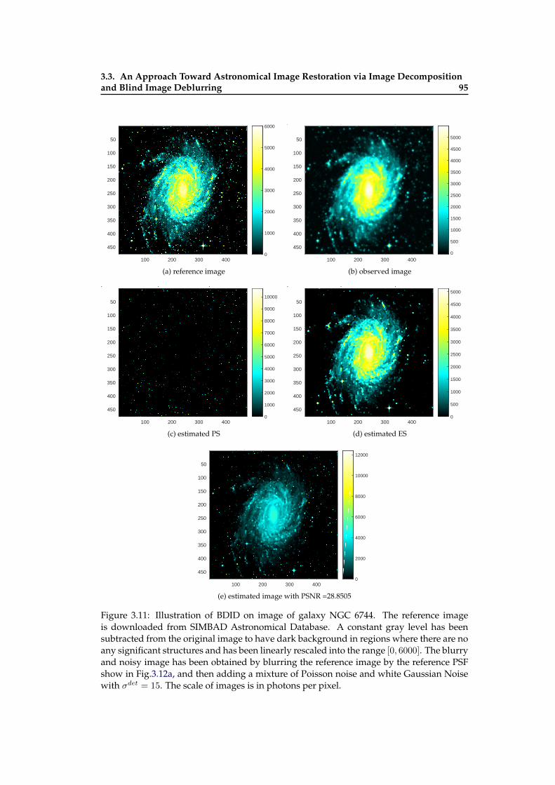
3.3. An Approach Toward Astronomical Image Restoration via Image Decompositionand Blind Image Deblurring 95
True Image: MIN = 0.0000, MAX = 6000.0000, MEAN = 597.6147, STD = 1107.5868
100 200 300 400
50
100
150
200
250
300
350
400
4500
1000
2000
3000
4000
5000
6000
(a) reference image
Observed Image: BSNR = 31.0464 SSIM = 0.1908 MIN = -58.4948, MAX = 5485.4474, MEAN = 597.7948, STD = 1021.6013
100 200 300 400
50
100
150
200
250
300
350
400
4500
500
1000
1500
2000
2500
3000
3500
4000
4500
5000
(b) observed imageEstimated Point Sources:
MIN = 0.0000, MAX = 10684.0544, MEAN = 25.7607, STD = 291.9372
100 200 300 400
50
100
150
200
250
300
350
400
4500
1000
2000
3000
4000
5000
6000
7000
8000
9000
10000
(c) estimated PS
Estimated Extended Sources: MIN = 0.0000, MAX = 5128.8258, MEAN = 516.7342, STD = 958.4979
100 200 300 400
50
100
150
200
250
300
350
400
4500
500
1000
1500
2000
2500
3000
3500
4000
4500
5000
(d) estimated ESEstimated Image: PSNR = 28.8187 SSIM = 0.4916
MIN = 0.0000, MAX = 12369.6244, MEAN = 542.4949, STD = 1011.3651
100 200 300 400
50
100
150
200
250
300
350
400
4500
2000
4000
6000
8000
10000
12000
(e) estimated image with PSNR =28.8505
Figure 3.11: Illustration of BDID on image of galaxy NGC 6744. The reference imageis downloaded from SIMBAD Astronomical Database. A constant gray level has beensubtracted from the original image to have dark background in regions where there are noany significant structures and has been linearly rescaled into the range [0, 6000]. The blurryand noisy image has been obtained by blurring the reference image by the reference PSFshow in Fig.3.12a, and then adding a mixture of Poisson noise and white Gaussian Noisewith σdet = 15. The scale of images is in photons per pixel.
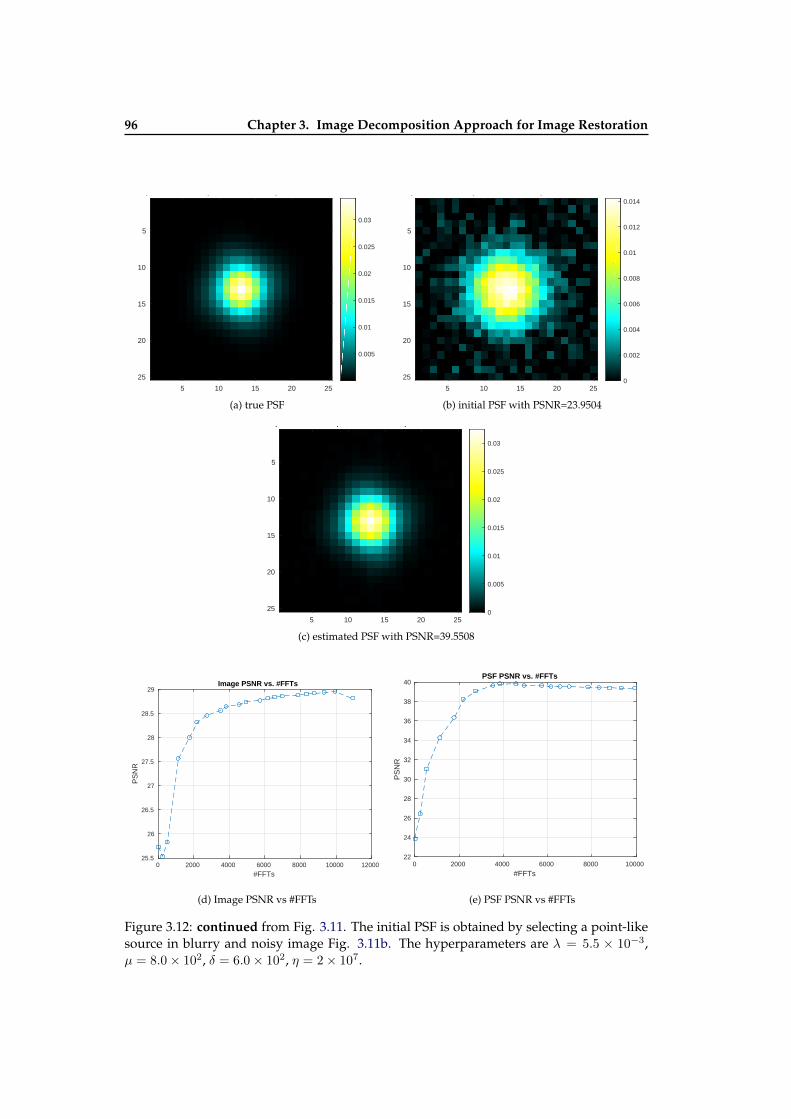
96 Chapter 3. Image Decomposition Approach for Image Restoration
True Image: MIN = 0.0000, MAX = 0.0341, MEAN = 0.0016, STD = 0.0045
5 10 15 20 25
5
10
15
20
25
0.005
0.01
0.015
0.02
0.025
0.03
(a) true PSF
Initial PSF: PSNR = 23.7648 MIN = 0.0000, MAX = 0.0143, MEAN = 0.0018, STD = 0.0030
5 10 15 20 25
5
10
15
20
25 0
0.002
0.004
0.006
0.008
0.01
0.012
0.014
(b) initial PSF with PSNR=23.9504Estimated PSF: PSNR = 39.3767
MIN = 0.0000, MAX = 0.0324, MEAN = 0.0017, STD = 0.0047
5 10 15 20 25
5
10
15
20
25 0
0.005
0.01
0.015
0.02
0.025
0.03
(c) estimated PSF with PSNR=39.5508
#FFTs0 2000 4000 6000 8000 10000 12000
PS
NR
25.5
26
26.5
27
27.5
28
28.5
29Image PSNR vs. #FFTs
(d) Image PSNR vs #FFTs
#FFTs0 2000 4000 6000 8000 10000
PS
NR
22
24
26
28
30
32
34
36
38
40PSF PSNR vs. #FFTs
(e) PSF PSNR vs #FFTs
Figure 3.12: continued from Fig. 3.11. The initial PSF is obtained by selecting a point-likesource in blurry and noisy image Fig. 3.11b. The hyperparameters are λ = 5.5 × 10⁻³,µ = 8.0× 10², δ = 6.0× 10², η = 2× 10⁷.

3.4. Conclusion and Perspective 97
3.4 Conclusion and Perspective
In this chapter, I have presented an approach toward restoration of astronomical imagesvia image decomposition and blind image deblurring techniques assuming that many as-tronomical scenes can be approximated by superimposition of mainly point-like sourcesand extended smooth sources. We can see that the restoration results on synthetic imagesin Fig. 3.1 and Fig.3.5 are promising; most of the point-like sources and the small disks arewell resolved without distorting the shapes and structures of the extended sources. Therestoration results on astronomical images from space telescope in Fig.3.9 and Fig.3.11 areslightly less satisfactory; however we can see certain gains in PSNR values. The possiblereasons for slightly less satisfactory results on these images could be that assumptions arenot very well satisfied by these images since they contain more complex structures. Fur-ther improvements to the proposed image restoration technique can be done by consider-ing more sophisticated image priors, especially for the complex structures in the extendedsources, and by an accurate estimation of the noise variances.
Even though here in this work, I used only PSNR metric for evaluating the qualityof image, but one should consider astrometry (precision of the position) and photometry(precision of the luminosity) as criteria to measure the quality of restoration. Depending onthe strength of the prior term (the values of the hyperparameters), the solutions obtainedfrom BDID are biased, thus one can improve the photometry of the estimated point-likesources by debiasing the final point-like sources map alone. Considering the detection ofpoint-like sources, a good tradeoff between false alarm and true detection should be foundby tuning the hyperparameters.
The astronomical images available at the astronomical database are not the raw im-ages directly obtained from ground-based imaging systems. They have been subjected tosequences of several preprocessing steps. In fact, they are constructed from multiple expo-sures of the same field with small shifts and rotations with respect to each other, commonlyreferred as “dithered” images. The common practice in astronomy is to resample (usingsome interpolation method) and align the multiple exposures, and then superimpose/co-add them to get the final image. This introduces highly correlated (colored) noise in the fi-nal image. Instead of superimposing directly the several aligned images to obtain the finalimage, one could apply multiframe blind image deblurring [Schulz 1993, Hom 2007] onthose several exposures of the same field, to achieve better results, of course with highercomputational budget than BDID. In the framework of the BDID, the multi-frame blindimage deblurring could be stated as:
x∗P ,x∗E ,h∗1, · · · ,h∗k = arg minxP ,xE ,h1,··· ,hk
1
2
K∑k=1
‖yk −Hk(xP + xE)‖2W k+ λ‖xP ‖1 + µ
∑i
φ(∇ixE)
+η
2
∑i
‖∇ihk‖22 + · · ·+ η
2
∑i
‖∇ihK‖22
such that xP ≥ 0, xE ≥ 0,
0 ≤ hk ≤ α, 1Thk = 1,∀k = 1, · · · ,K.
where yk, hk and W k are the k-th observed image, the associated PSF and the inverseof noise covariance matrix, respectively. One could account for translations of the blurryand noisy images by shifted PSFs, and if one consider shift-variant blur operator, then onecould also even account for rotation between the images. Solving this problem in the wayas described in Section 3.3.4 is possible when K is not very large, otherwise one could anonline-scheme similar to the one presented in [Harmeling 2009].

98 Chapter 3. Image Decomposition Approach for Image Restoration
3.5 Summary
The chapter presented a general discuss on image decomposition, different decompositionmethods from synthesis and analysis based approaches, and the fruitfulness of decompo-sition in image restoration. Further, this chapter presented a detailed overview of blindimage deblurring methods, and proposed a blind image deblurring algorithm via imagedecomposition (BDID) for restoration of astronomical image. The results from BDID onthe synthetically created images are promising with hope that the method can be furtherimproved to handle real astronomical images.
CHAPTER 4
Restoration of Images withShift-Variant Blur
Everything should be made as simple as possible, but not simpler.– Albert Einstein
Contents4.1 Introduction . . . . . . . . . . . . . . . . . . . . . . . . . . . . . . . . . . . . . . 1004.2 Implementation and Cost Complexity Details of Shift-Variant Blur Operator . 1014.3 Shift-Variant Image Deblurring . . . . . . . . . . . . . . . . . . . . . . . . . . . 1054.4 Estimation of Shift-Variant Blur . . . . . . . . . . . . . . . . . . . . . . . . . . . 107
4.4.1 Characteristics of Blur due to Optical Aberrations . . . . . . . . . . . . 1074.4.2 Estimation of Shift-Variant Blur due to Optical Aberrations . . . . . . 1094.4.3 Shift-Variant PSFs Calibration . . . . . . . . . . . . . . . . . . . . . . . 111
4.5 Conclusion . . . . . . . . . . . . . . . . . . . . . . . . . . . . . . . . . . . . . . 1134.6 Summary . . . . . . . . . . . . . . . . . . . . . . . . . . . . . . . . . . . . . . . 114
100 Chapter 4. Restoration of Images with Shift-Variant Blur
Abstract
In many practical imaging systems, the blur is not stationary throughout the field-of-view,for example, wide-field-view imaging in astronomy, along the depth in microscopic imag-ing, and motion blur in photography. The images captured by such systems suffer fromshift-variant blur degradation. However, it is essential in many applications to have highresolution images. Most of the classical image deblurring methods are based on shift-invariant blur assumption, and they cannot improve the quality of images suffering fromshift-variant blur. In this chapter, we will see a detailed discussion on shift-variant im-age deblurring. The chapter will start with a recall of shift-variant blur model discussed inChapter 1, and then it will provide the detailed implementational overview of shift-variantblur operator based on PSF interpolation. It will also discuss the advantages of using thisparticular model. Afterwards the two main steps: the image deblurring and the PSF es-timation, for blind image deblurring in the case of shift-variant blur, will be presented.The results from the two steps are promising, and indicate that we can achieve good re-sults in the near future from the blind image deblurring method combining the two stepspresented in this chapter.
4.1 Introduction
In many imaging systems the degradation of the acquired image due to blur and noise isinevitable. In Chapter 1, we saw three fundamental causes of blur: i) the media betweenthe object and image plane, ii) finite aperture of the imaging system, and iii) finite exposuretime. Among these three fundamental causes, the blur due to the second cause is shift-invariant, whereas the blur due to the remaining two causes can result in shift-variantblur. For narrow field-of-view imaging, the blur due to the first cause is almost shift-invariant, while for wide field-of-view imaging, the blur due to it is shift-variant in manyimaging situations. For examples, in case of shallow depth of focus; for low cost camerasthe lens produce optical aberrations; in long distance imaging the effect of atmosphericturbulences is added; in microscopy, the shallow depth of focus and optical aberrations;all these causes contribute to shift-variant blur. In bright light situation, a small integrationtime is sufficient to capture a good contrast image, thus blur due to the third reason isavoidable, but, in low lighting condition, the chances of blur due to motion is high, andthe resulting blur is mostly shift-variant in the field of view.
The quality/resolution of the images suffering from shift-variant blur can be improvedsignificantly by digital image deblurring methods provided that the shift-variant PSF isknown beforehand or can be estimated accurately by some mean. The quality of the re-stored image is dependent upon the accuracy of the given PSFs, and if one knows the PSFsat the every pixel location, one can achieve high quality image, of course, also dependenton the signal-to-noise ratio. However, in many imaging situations, the knowledge of thePSF at the every pixel location is practically impossible, except in the case where the PSFis described by a parametric model. Image blurring and deblurring are computationallyintensive if one considers the PSF at the every pixel location. In many situations, the blurvaries smoothly in the field of view, except in the cases of shallow depth of focus where oneobject is completely in focus, and surrounding objects are completely defocused (as shownin Fig.4.1a) or the focused object in the image is moving with respect to the surroundings(as shown in Fig. 4.1b). In the latter cases, the blurred image cannot be related to a singleplanar crisp image, but can be considered as composed of several layers of planar crisp im-ages with their associated alpha matte (i.e., opacity image), see [Porter 1984, Wang 2008],
4.2. Implementation and Cost Complexity Details of Shift-Variant Blur Operator 101
and image deblurring of such images is very challenging task. In this thesis, I limit mystudy to the cases where blur is varying smoothly (as shown in Fig. 4.1c), which is alreadya difficult problem. With smooth variation of blur, it is sufficient to have a grid of PSFs(locations in the field of view where PSFs are sampled), depending upon how smoothlythe PSFs are varying, and then the PSFs between grid points can be approximated by inter-polation methods. In Chapter 1, we saw some shift-variant blurring approximations otherthan PSFs interpolation, however, in those models we cannot simply impose the normaliza-tion and positivity constraint. Moreover, on the low-rank approximation on PSFs modesapproach cannot be used in straightforward way or can be computationally expensive ifone wants to impose certain constraints on the PSFs in estimation methods, which will wediscuss in upcoming sections. Thus, in my work, I consider the PSFs interpolation approx-imation for shift-variant blur. With this approach, the blurring operation is simplified bythe following separable approximation as described in Chapter 1:
H ≈∑p∈GP
conv(kp) diag(wp) (4.1)
where GP denotes the set of all points on a given grid of PSFs, conv(kp) denotes the discreteconvolution matrix with blur kernel kp at the pth grid point, diag(wp) is a diagonal matrixwhose diagonal is given by the interpolation weight vector wp around the pth grid point,which has a limited support. The convolution can be efficiently done in Fourier domainusing Fast Fourier Transform (FFT) algorithms, and thus the total computational cost ofthe above blurring operator depends upon the number of dimensions along which thePSFs vary, and on the interpolation order used for a given grid of PSFs. In this chapter,I demonstrate only 2D image deblurring with bilinear interpolation weights. In the nextsection we will see the implementation aspect of the blur operator and its complexity indetail.
4.2 Implementation and Cost Complexity Details of Shift-Variant Blur Operator
Let us consider P 2D PSFs of equal support of size, t = tx×ty , pixels uniformly sampled ona rectangular grid within the support of a given 2D image x of size, m = mx ×my , pixels.From an implementation point of view, the blur operator in Eq. (4.1) can be written:
H = R
P∑p=1
Zp Hp Wp C(x)p (4.2)
where C(x)p ∈ Rl×m is a cropping operator, which extracts pth 2D image patch of size l =
lx× ly matching to the support of the interpolation weights matrix Wp = diag(wp) ∈ Rl×l.The matrix Hp = conv(kp) ∈ R[(lx+tx−1)×(ly+ty−1)]×[lx×ly ] is a discrete convolution matrixcorresponding to the PSF at pth grid that can be diagonalized by Fourier transform:
Hp = F−1 diag(kp) F E(x) (4.3)
wherekp = F E(k)kp (4.4)
The matrices E(k) ∈ R[(lx+tx−1)×(ly+ty−1)]×[tx×ty ] and E(x) ∈ R[(lx+tx−1)×(ly+ty−1)]×[lx×ly ]
are extension operators, which zero-pad the PSF and the image patch to the size [(lx +
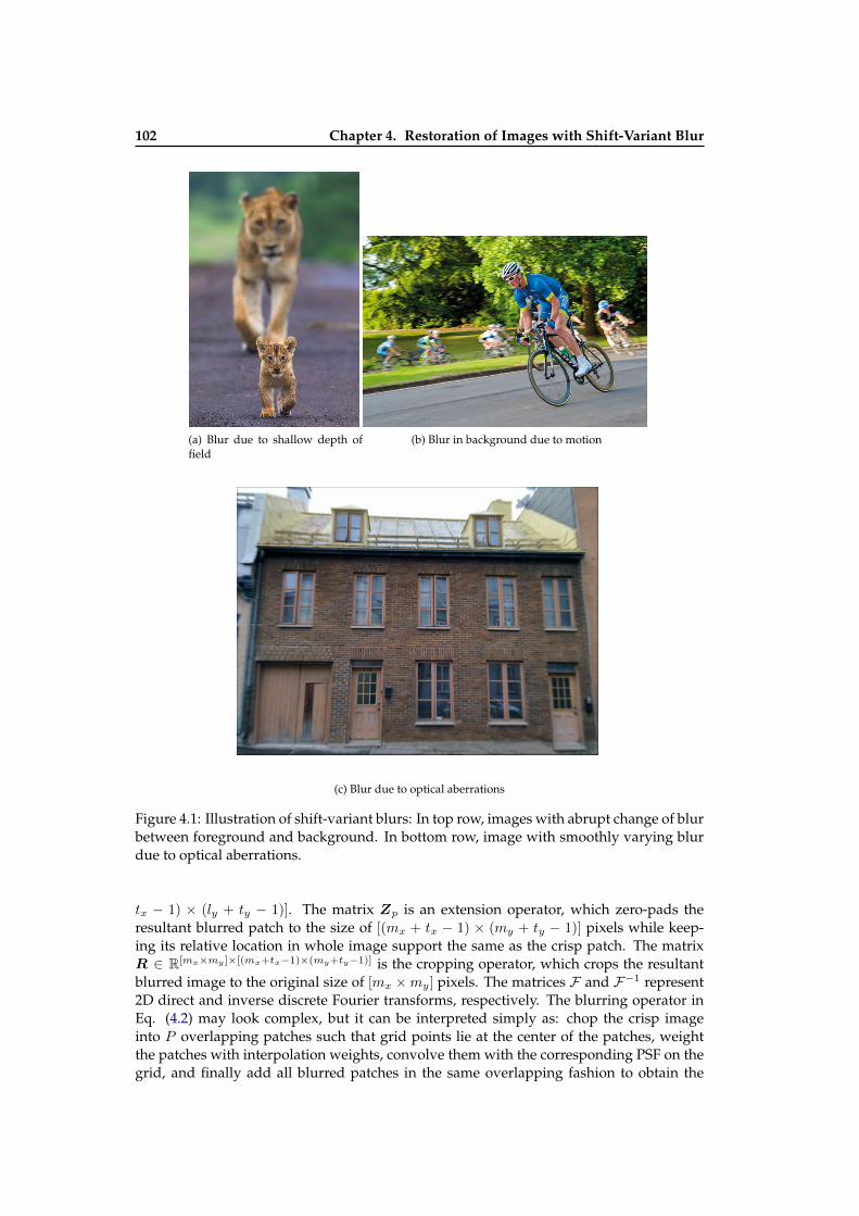
102 Chapter 4. Restoration of Images with Shift-Variant Blur
(a) Blur due to shallow depth offield
(b) Blur in background due to motion
(c) Blur due to optical aberrations
Figure 4.1: Illustration of shift-variant blurs: In top row, images with abrupt change of blurbetween foreground and background. In bottom row, image with smoothly varying blurdue to optical aberrations.
tx − 1) × (ly + ty − 1)]. The matrix Zp is an extension operator, which zero-pads theresultant blurred patch to the size of [(mx + tx − 1) × (my + ty − 1)] pixels while keep-ing its relative location in whole image support the same as the crisp patch. The matrixR ∈ R[mx×my ]×[(mx+tx−1)×(my+ty−1)] is the cropping operator, which crops the resultantblurred image to the original size of [mx ×my] pixels. The matrices F and F−1 represent2D direct and inverse discrete Fourier transforms, respectively. The blurring operator inEq. (4.2) may look complex, but it can be interpreted simply as: chop the crisp imageinto P overlapping patches such that grid points lie at the center of the patches, weightthe patches with interpolation weights, convolve them with the corresponding PSF on thegrid, and finally add all blurred patches in the same overlapping fashion to obtain the
4.2. Implementation and Cost Complexity Details of Shift-Variant Blur Operator 103
blurred image. Figure 4.2 illustrate the blurring operation following the operator in Eq.(4.2).
In the PSF estimation step in blind image deblurring solved by alternating minimization,the blurring operator formed from image is required. It can be analogously written as:
X = R
P∑p=1
Zp X p C(k)p (4.5)
where C(k)p ∈ R[tx×ty ]×[P×(tx×ty)] extracts the pth PSF from a column vector containing all
P PSFs. The matrix X p ∈ R[(lx+tx−1)×(ly+ty−1)]×[tx×ty ] is the discrete convolution matrixformed from the weighted image patch xp = Wp C
(x)p x than can be diagonalized by
Fourier transform:X p = F−1 diag(xp) E
(k) (4.6)
wherexp = F E(x) xp (4.7)
The matrices E(k) and E(x) are extension operators, which zero-pad the weighted imagepatch xp and the PSF kp to the size [(lx + tx − 1)× (lx + tx − 1)]. The operators Zp andRhave the same meanings as in Eq. (4.2).
In Bayesian inference framework, the image deblurring and the PSF estimation meth-ods boil down to optimization problems, thus they often require to evaluate the adjointoperators HT and XT . Following the conventions used in the definition of the blur oper-atorsH andX , their adjoints are written as:
HT =
P∑p=1
C(x)p
TWp HT
p ZTp R
T (4.8)
and
XT =
P∑p=1
C(k)p
TX Tp Z
Tp R
T (4.9)
where
HTp = E(x)TF−1 diag(kp) F (4.10)
and
X T = E(k)TF−1 diag(xp) F (4.11)
where (·) represents the complex conjugate of the input argument.Now, given the implementational details of the blur operator Eq.(4.2), we can express
accurately its complexity. Though the blur operators are written considering only 2D im-ages and first-order interpolation weights, here I show the complexity for a general case,where d represents the dimension along which PSFs vary and o is the order of interpo-lation. With a crisp image of size m pixels, P PSFs of equal supports of size t pixels ona rectangular grid, the number of pixels inside a grid cell is on average m/P . Due tothe overlap of interpolation weights, each convolution in Eq. (4.2) is carried on (o + 1)d
cells. These convolutions are computed using FFTs with an appropriate padding witht1/d zeros along each dimension, assuming that PSFs have identical size in each dimen-sions. The FFTs are then computed on an area of about [(o+ 1)× (m/P )1/d + t1/d]d pixels.Since the whole operator involves P such computations, the total complexity is of order
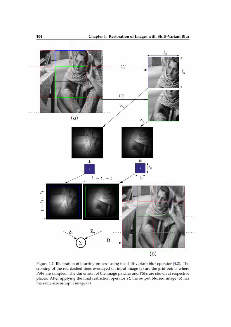
104 Chapter 4. Restoration of Images with Shift-Variant Blur
(a)
(b)
Figure 4.2: Illustration of blurring process using the shift-variant blur operator (4.2). Thecrossing of the red dashed lines overlayed on input image (a) are the grid points wherePSFs are sampled. The dimension of the image patches and PSFs are shown at respectiveplaces. After applying the final restriction operator R, the output blurred image (b) hasthe same size as input image (a).
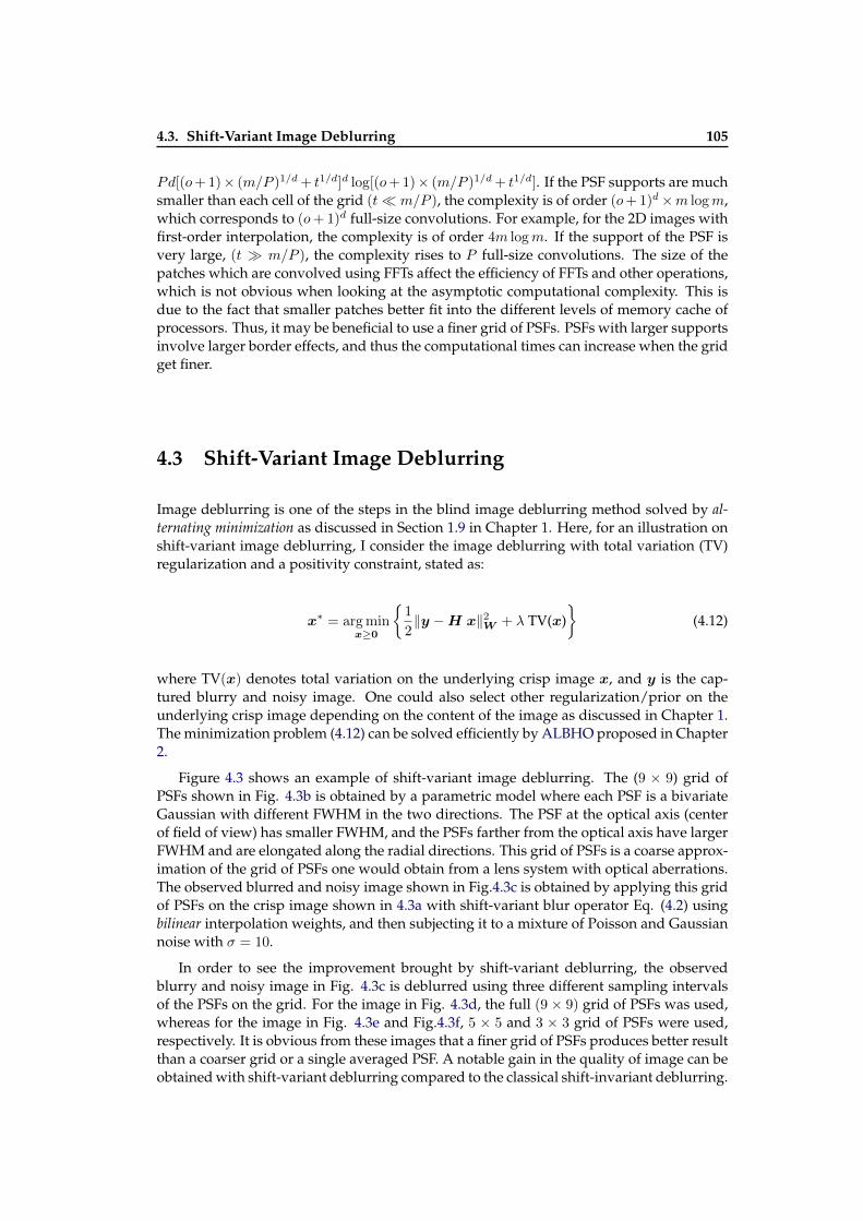
4.3. Shift-Variant Image Deblurring 105
Pd[(o+ 1)× (m/P )1/d + t1/d]d log[(o+ 1)× (m/P )1/d + t1/d]. If the PSF supports are muchsmaller than each cell of the grid (t m/P ), the complexity is of order (o+ 1)d×m logm,which corresponds to (o+ 1)d full-size convolutions. For example, for the 2D images withfirst-order interpolation, the complexity is of order 4m logm. If the support of the PSF isvery large, (t m/P ), the complexity rises to P full-size convolutions. The size of thepatches which are convolved using FFTs affect the efficiency of FFTs and other operations,which is not obvious when looking at the asymptotic computational complexity. This isdue to the fact that smaller patches better fit into the different levels of memory cache ofprocessors. Thus, it may be beneficial to use a finer grid of PSFs. PSFs with larger supportsinvolve larger border effects, and thus the computational times can increase when the gridget finer.
4.3 Shift-Variant Image Deblurring
Image deblurring is one of the steps in the blind image deblurring method solved by al-ternating minimization as discussed in Section 1.9 in Chapter 1. Here, for an illustration onshift-variant image deblurring, I consider the image deblurring with total variation (TV)regularization and a positivity constraint, stated as:
x∗ = arg minx≥0
1
2‖y −H x‖2W + λ TV(x)
(4.12)
where TV(x) denotes total variation on the underlying crisp image x, and y is the cap-tured blurry and noisy image. One could also select other regularization/prior on theunderlying crisp image depending on the content of the image as discussed in Chapter 1.The minimization problem (4.12) can be solved efficiently by ALBHO proposed in Chapter2.
Figure 4.3 shows an example of shift-variant image deblurring. The (9 × 9) grid ofPSFs shown in Fig. 4.3b is obtained by a parametric model where each PSF is a bivariateGaussian with different FWHM in the two directions. The PSF at the optical axis (centerof field of view) has smaller FWHM, and the PSFs farther from the optical axis have largerFWHM and are elongated along the radial directions. This grid of PSFs is a coarse approx-imation of the grid of PSFs one would obtain from a lens system with optical aberrations.The observed blurred and noisy image shown in Fig.4.3c is obtained by applying this gridof PSFs on the crisp image shown in 4.3a with shift-variant blur operator Eq. (4.2) usingbilinear interpolation weights, and then subjecting it to a mixture of Poisson and Gaussiannoise with σ = 10.
In order to see the improvement brought by shift-variant deblurring, the observedblurry and noisy image in Fig. 4.3c is deblurred using three different sampling intervalsof the PSFs on the grid. For the image in Fig. 4.3d, the full (9 × 9) grid of PSFs was used,whereas for the image in Fig. 4.3e and Fig.4.3f, 5 × 5 and 3 × 3 grid of PSFs were used,respectively. It is obvious from these images that a finer grid of PSFs produces better resultthan a coarser grid or a single averaged PSF. A notable gain in the quality of image can beobtained with shift-variant deblurring compared to the classical shift-invariant deblurring.
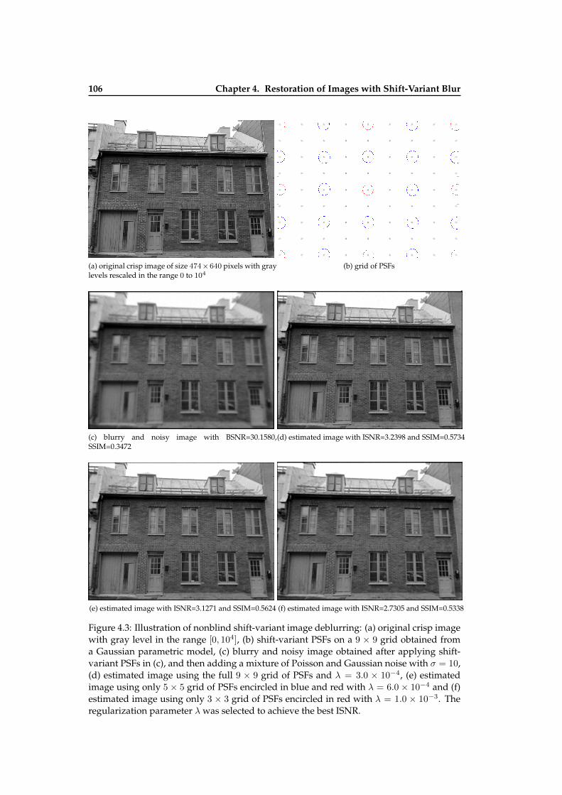
106 Chapter 4. Restoration of Images with Shift-Variant Blur
(a) original crisp image of size 474×640 pixels with graylevels rescaled in the range 0 to 104
(b) grid of PSFs
(c) blurry and noisy image with BSNR=30.1580,SSIM=0.3472
(d) estimated image with ISNR=3.2398 and SSIM=0.5734
(e) estimated image with ISNR=3.1271 and SSIM=0.5624 (f) estimated image with ISNR=2.7305 and SSIM=0.5338
Figure 4.3: Illustration of nonblind shift-variant image deblurring: (a) original crisp imagewith gray level in the range [0, 104], (b) shift-variant PSFs on a 9 × 9 grid obtained froma Gaussian parametric model, (c) blurry and noisy image obtained after applying shift-variant PSFs in (c), and then adding a mixture of Poisson and Gaussian noise with σ = 10,(d) estimated image using the full 9 × 9 grid of PSFs and λ = 3.0 × 10⁻⁴, (e) estimatedimage using only 5 × 5 grid of PSFs encircled in blue and red with λ = 6.0 × 10⁻⁴ and (f)estimated image using only 3 × 3 grid of PSFs encircled in red with λ = 1.0 × 10⁻³. Theregularization parameter λ was selected to achieve the best ISNR.
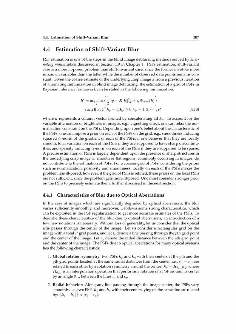
4.4. Estimation of Shift-Variant Blur 107
4.4 Estimation of Shift-Variant Blur
PSF estimation is one of the steps in the blind image deblurring methods solved by alter-nating minimization discussed in Section 1.9 in Chapter 1. PSFs estimation, shift-variantcase is a more ill-posed problem than shift-invariant case, since the former involves moreunknown variables than the latter while the number of observed data points remains con-stant. Given the coarse estimate of the underlying crisp image x from a previous iterationof alternating minimization in blind image deblurring, the estimation of a grid of PSFs inBayesian inference framework can be stated as the following minimization:
k∗ = arg mink
1
2‖y −X k‖2W + η Ψprior(k)
such that 1Tkp = 1,kp ≥ 0,∀p = 1, 2, · · · , P. (4.13)
where k represents a column vector formed by concatenating all kp. To account for thevariable attenuation of brightness in images, e.g., vignetting effect, one can relax the nor-malization constraint on the PSFs. Depending upon one’s belief about the characteristic ofthe PSFs, one can impose a prior on each of the PSFs on the grid, e.g., smoothness inducingsquared `2-norm of the gradient of each of the PSFs, if one believes that they are locallysmooth, total variation on each of the PSFs if they are supposed to have sharp discontinu-ities, and sparsity inducing `1-norm on each of the PSFs if they are supposed to be sparse.A precise estimation of PSFs is largely dependent upon the presence of sharp structures inthe underlying crisp image x: smooth or flat regions, commonly occurring in images, donot contribute to the estimation of PSFs. For a coarser grid of PSFs, considering the priorssuch as normalization, positivity and smoothness, locally on each of the PSFs makes theproblem less ill-posed; however, if the grid of PSFs is refined, these priors on the local PSFsare not sufficient, since the problem gets more ill-posed. One must consider stronger prioron the PSFs to precisely estimate them, further discussed in the next section.
4.4.1 Characteristics of Blur due to Optical Aberrations
In the case of images which are significantly degraded by optical aberrations, the blurvaries sufficiently smoothly, and moreover, it follows some strong characteristics, whichcan be exploited in the PSF regularization to get more accurate estimates of the PSFs. Todescribe these characteristics of the blur due to optical aberrations, an introduction of afew new notations is necessary. Without loss of generality, let us consider that the opticalaxis passes through the center of the image. Let us consider a rectangular grid on theimage with a total P grid points, and let lp denote a line passing through the pth grid pointand the center of the image. Let rp denote the radial distance between the pth grid pointand the center of the image. The PSFs due to optical aberrations for many optical systemshas the following characteristics:
1. Global rotation symmetry: two PSFs kp and kq with their centers at the pth and theqth grid points located at the same radial distances from the center, i.e., rp = rq , arerelated to each other by a rotation symmetry around the center: kp = Rθp,qkq , whereRθp,q is an interpolation operation that performs a rotation of a PSF around its centerby an angle θp,q between the lines lp and lq .
2. Radial behavior: Along any line passing through the image center, the PSFs varysmoothly, i.e., two PSFs kp and kq with their centers lying on the same line are relatedby: ‖kp − kq‖22 ∝ |rp − rq|.
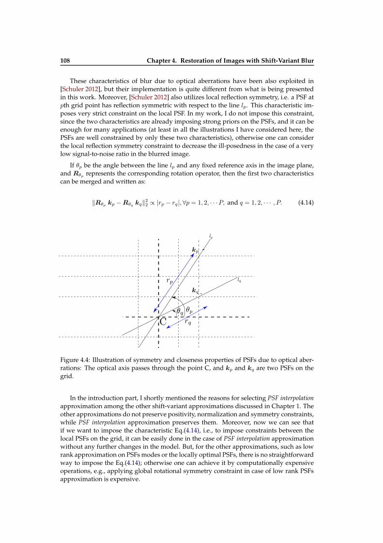
108 Chapter 4. Restoration of Images with Shift-Variant Blur
These characteristics of blur due to optical aberrations have been also exploited in[Schuler 2012], but their implementation is quite different from what is being presentedin this work. Moreover, [Schuler 2012] also utilizes local reflection symmetry, i.e. a PSF atpth grid point has reflection symmetric with respect to the line lp. This characteristic im-poses very strict constraint on the local PSF. In my work, I do not impose this constraint,since the two characteristics are already imposing strong priors on the PSFs, and it can beenough for many applications (at least in all the illustrations I have considered here, thePSFs are well constrained by only these two characteristics), otherwise one can considerthe local reflection symmetry constraint to decrease the ill-posedness in the case of a verylow signal-to-noise ratio in the blurred image.
If θp be the angle between the line lp and any fixed reference axis in the image plane,and Rθp represents the corresponding rotation operator, then the first two characteristicscan be merged and written as:
‖Rθp kp −Rθq kq‖22 ∝ |rp − rq|,∀p = 1, 2, · · ·P, and q = 1, 2, · · · , P. (4.14)
Figure 4.4: Illustration of symmetry and closeness properties of PSFs due to optical aber-rations: The optical axis passes through the point C, and kp and kq are two PSFs on thegrid.
In the introduction part, I shortly mentioned the reasons for selecting PSF interpolationapproximation among the other shift-variant approximations discussed in Chapter 1. Theother approximations do not preserve positivity, normalization and symmetry constraints,while PSF interpolation approximation preserves them. Moreover, now we can see thatif we want to impose the characteristic Eq.(4.14), i.e., to impose constraints between thelocal PSFs on the grid, it can be easily done in the case of PSF interpolation approximationwithout any further changes in the model. But, for the other approximations, such as lowrank approximation on PSFs modes or the locally optimal PSFs, there is no straightforwardway to impose the Eq.(4.14); otherwise one can achieve it by computationally expensiveoperations, e.g., applying global rotational symmetry constraint in case of low rank PSFsapproximation is expensive.
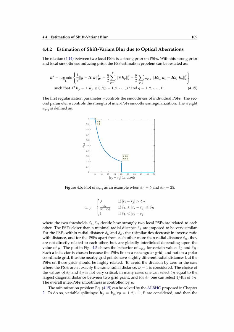
4.4. Estimation of Shift-Variant Blur 109
4.4.2 Estimation of Shift-Variant Blur due to Optical Aberrations
The relation (4.14) between two local PSFs is a strong prior on PSFs. With this strong priorand local smoothness inducing prior, the PSF estimation problem can be restated as:
k∗ = arg mink
1
2‖y −X k‖2W +
η
2
P∑p=1
‖∇kp‖22 +µ
2
∑p,q
ωp,q ‖Rθp kp −Rθq kq‖22
such that 1Tkp = 1,kp ≥ 0,∀p = 1, 2, · · · , P and q = 1, 2, · · · , P. (4.15)
The first regularization parameter η controls the smoothness of individual PSFs. The sec-ond parameter µ controls the strength of inter-PSFs smoothness regularization. The weightωp,q is defined as:
Figure 4.5: Plot of ωp,q as an example when δL = 5 and δH = 25.
ωi,j =
0 if |ri − rj | > δHδL
|ri−rj | if δL ≤ |ri − rj | ≤ δH1 if δL < |ri − rj |
where the two thresholds δL, δH decide how strongly two local PSFs are related to eachother. The PSFs closer than a minimal radial distance δL are imposed to be very similar.For the PSFs within radial distance δL and δH , their similarities decrease in inverse ratiowith distance, and for the PSFs apart from each other more than radial distance δH , theyare not directly related to each other, but, are globally interlinked depending upon thevalue of µ. The plot in Fig. 4.5 shows the behavior of ωp,q for certain values δL and δH .Such a behavior is chosen because the PSFs lie on a rectangular grid, and not on a polarcoordinate grid, thus the nearby grid points have slightly different radial distances but thePSFs on those grids should be highly related. To avoid the division by zero in the casewhere the PSFs are at exactly the same radial distance, ω = 1 is considered. The choice ofthe values of δL and δH is not very critical; in many cases one can select δH equal to thelargest diagonal distance between two grid point, and for δL one can select 1/4th of δH .The overall inter-PSFs smoothness is controlled by µ.
The minimization problem Eq. (4.15) can be solved by the ALBHO proposed in Chapter2. To do so, variable splittings: hp = kp,∀p = 1, 2, · · · , P are considered, and then the
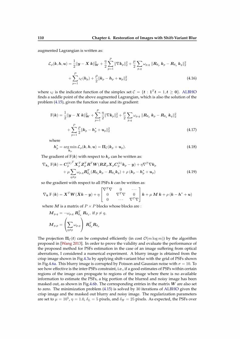
110 Chapter 4. Restoration of Images with Shift-Variant Blur
augmented Lagrangian is written as:
Lρ(k,h,u) =1
2‖y −X k‖2W +
η
2
P∑p=1
‖∇kp‖22 +µ
2
∑p,q
ωp,q ‖Rθp kp −Rθq kq‖22
+
P∑p=1
ιC(hp) +ρ
2‖kp − hp + up‖22 (4.16)
where ιC is the indicator function of the simplex set C = t : 1T t = 1, t ≥ 0. ALBHOfinds a saddle point of the above augmented Lagrangian, which is also the solution of theproblem (4.15), given the function value and its gradient:
F(k) =1
2‖y −X k‖2W +
P∑p=1
η
2‖∇kp‖22 +
µ
2
∑p,q
ωp,q ‖Rθp kp −Rθq kq‖22
+
P∑p=1
ρ
2‖kp − h∗p + up‖22 (4.17)
where
h∗p = arg minhp
Lρ(k,h,u) = ΠC(kp + up). (4.18)
The gradient of F(k) with respect to kp can be written as:
∇kp F(k) = C(k)p
TXTpZ
TpR
TW (RZpXpC(k)p kp − y) + η∇T∇kp
+ µ∑q 6=p
ωp,qRTθp(Rθpkp −Rθqkq) + ρ (kp − h∗p + up) (4.19)
so the gradient with respect to all PSFs k can be written as:
∇k F (k) = XTW (Xk − y) + η
∇T∇ 0 · · ·0 ∇T∇ 0
0 · · · ∇T∇
k + µM k + ρ (k − h∗ + u)
whereM is a matrix of P × P blocks whose blocks are :
Mp,q = −ωp,q RTθp Rθq , if p 6= q,
Mp,p =
∑q 6=p
ωp,q
RTθpRθp
The projection ΠC(t) can be computed efficiently (in cost O(m logm)) by the algorithmproposed in [Wang 2013]. In order to prove the validity and evaluate the performance ofthe proposed method for PSFs estimation in the case of an image suffering from opticalaberrations, I considered a numerical experiment. A blurry image is obtained from thecrisp image shown in Fig.4.3a by applying shift-variant blur with the grid of PSFs shownin Fig.4.6a. This blurry image is corrupted by Poisson and Gaussian noise with σ = 10. Tosee how effective is the inter-PSFs constraint, i.e., if a good estimates of PSFs within certainregions of the image can propagate to regions of the image where there is no availableinformation to estimate the PSFs, a big portion of the blurred and noisy image has beenmasked out, as shown in Fig.4.6b. The corresponding entries in the matrix W are also setto zero. The minimization problem (4.15) is solved by 30 iterations of ALBHO given thecrisp image and the masked out blurry and noisy image. The regularization parametersare set to µ = 105, η = 1.0, δL = 5 pixels, and δH = 25 pixels. As expected, the PSFs over

4.4. Estimation of Shift-Variant Blur 111
the whole field of view are fairly estimated, except at the corners, which are relatively farfrom the regions where data are available. The estimated PSFs on the grid are shown inFig. 4.6c and their corresponding PSNR value is shown in Fig.4.6d at the same relativepositions. The higher the value of µ, the stronger the inter-PSFs constraint, and goodestimate of PSFs propagate to regions where there is no information for the estimation.
(a) reference grid of PSFs (b) restricted portion of blurry and noisy image
(c) estimated grid of PSFs
15
20
25
30
35
40
(d) PSNR of estimated 9× 9 grid of PSFs
Figure 4.6: Out of field of view PSFs estimation for blur due to optical aberrations
4.4.3 Shift-Variant PSFs Calibration
In the above illustrations, the grid of shift-variant PSFs is simulated using a bivariate Gaus-sian model. In order to get close experience of the PSFs due to optical aberrations, I didan experiment in Imaging and Optical Design laboratory under the supervision of ThierryLépine (an assistant Professor at Institut d’Optique). The objective was to capture imagesin a controlled environment with a simple lens camera, calibrate the PSF of this simplecamera, and compare the experimental PSFs with the PSFs simulated by Zemax opticaldesign software 1.
The experimental setup scheme is shown in Fig.4.7. The camera selected was THEIMAGINGSOURCE DMK 41 monochrome camera with pixels size 4.65× 4.65 µm2, and amatrix of 1280×960 pixels. This is an industrial grade camera that was selected for its low
1Zemax optical design software is industry standard design and simulation software for optical and illumi-nation designers, and researchers. http://www.zemax.com/.
112 Chapter 4. Restoration of Images with Shift-Variant Blur
Figure 4.7: Experimental setup scheme for PSFs calibration.
noise performance and simplicity to use with its interface to the computer. The lens wasa achromatic doublet with focal length of 100 mm. This lens was suggested by ThierryLépine after a few simulations on Zemax to see if it introduces sufficient shift-variant blurfor our demonstration purpose, and it was selected to be achromatic because we did notwant chromatic aberrations in the captured images. Also, to avoid any chromatic aberra-tion, a red filter with bandpass around 600 nm was placed before the CCD sensor. The exitpupil was selected to be circular with diameter of 10 mm. This size of pupil was selectedso that the diffraction limited PSF on the optical axis is not undersampled (i.e. it coversat least 2 pixels on the sensor). I selected a LCD screen to display the scenes instead ofusing the scenes printed on paper because the print quality was not good enough on theprinter at hand. Thus, the scenes were displayed at their native resolution on a mobilephone LCD display of pixel resolution 1920 × 1080 with 445 pixels per inch (i.e. pixelsize of 57.07 × 57.07 µ2m). The top left corner of the scene (screen) was approximatelyadjusted at optical axis of the whole imaging system. We can see that the pixel size of thescreen is almost 10 times bigger than the pixel size of camera sensor, thus in order to havea magnification factor of almost one between the scene and the captured image, the objectdistance was adjusted to be 1200mm, and the image distance was 110mm. Since the objectdistance was at least 10 times larger than the image distance, a single pixel in the scene (onthe screen) could be considered as a point source when seen from the optical center. Allthe images were captured in a darkroom to avoid any stray light that could corrupt themeasurements.
In the experiment for the PSF calibration, I captured different target patterns, such aspoint sources on dark background, and random noise pattern. However, for the reasondiscussed below, I finally used only the target pattern with point sources for the final cal-ibration. The captured image shown in Fig. 4.8b shows that the imaging process wasquite noisy even the gamma gain of the camera was kept at lower value. Moreover thedark background of the captured images have some nonuniform camera offset. This isdue to the fact that the LCD screen are backlit. In order to do precisely the PSF calibrationone should be able suppress/handle the noise and the nonuniform background offset. Inthe case of calibration pattern image containing point sources, this task turns out to berelatively easier because there is a large space between the point sources, and one couldmask out the background leaving only the point sources by using morphological dilations.

4.5. Conclusion 113
The background corrected captured image is shown in Fig. 4.9a. However, estimating thebackground offset in images, which do not have a dark background is a more difficult task.Before doing the final calibration, one has also to align the reference images with respectthe captured images, since the captured images are a portion of a bigger reference imagesand there are always some affine transform involved between them. In this work, thealignment and transformation of the reference image was done using MATLAB “ControlPoint Registration” method, where one selects a few corresponding points in the two im-ages, and then by the function “fitgeotrans” one gets the corresponding affine transformto be applied on the reference image. In the case of target pattern with random noise, itbecame difficult to align it even with some alignment pattern on it, and due to the affinetransform (involving interpolation) the crisp random pattern became slightly blurry.
Once the background corrected captured image and the aligned reference image of thepoint sources was available, a 21 × 21 grid of PSFs was estimated by the PSF estimationmethod presented in Section 4.4.2. The grid of PSFs at the four corners of the field of vieware shown in Fig.4.9b. The regularization parameters used in the estimation are µ = 102,η = 1.0, δL = 5 and δH = 15. Since, in this captured image, point sources are avail-able throughout the field of view, the regularization parameters are smaller than that isbeing used in the illustration in Fig. 4.4.2. With this estimated (calibrated) grid of PSFsshown in Fig.4.9b, an image shown in Fig.4.10a was deblurred using the shift-variant im-age deblurring method described in Section 4.3. The regularization parameter was set tobe λ = 5.0× 10⁻⁴
Comparing the captured image shown in the Fig. 4.9a and the estimated grid of PSFsshown in Fig.4.9b, we can say that the calibrated grid of PSFs is in good accordance withthe captured PSFs of the imaging system used in the experiment. This is also supportedby the results of deblurring shown in Fig.4.10, 4.11 and 4.12. We can see that the capturedblurry and noisy images have been restored with a quite good quality. For example, inFig.4.10, the regions marked by the red patches 1 and 2, are well restored, however, inthe region in patch 3, the blur is quite heavy compared to the signal-to-noise ratio. Also,one can notice that deblurred images contain some feeble vertical traces on the uniformregions. This is due to the fact that the protective film on the LCD screen had some finetraces on it, which became obvious after deblurring the captured image.
The simulated PSFs by Zemax have smaller support (are less spread out) than whatis being captured by the camera. This could happen due to several reasons; may be thecamera was not perfectly focused, and the spread in PSFs are due to some defocus; back litLCD screen create some diffusion of light, making the point sources a little hazy; the planeof the LCD screen and the CCD sensor were not perfectly perpendicular to the optical axis.All these causes contribute to some extra blur in the captured image than the simulatedPSFs.
4.5 Conclusion
In many practical imaging systems, the blur is mostly shift-variant; thus, shift-variant im-age deblurring is essential for those applications as it can produce better quality of imagesthan the shift-invariant deblurring. Considering a different PSF at each pixel location isredundant and this leads to computationally expensive blurring operations. For manyimaging situations, the blur varies smoothly throughout the field-of-view, thus one cansignificantly reduce the computation cost of shift-variant blurring by considering separa-ble linear approximation, without loosing significantly the accuracy of the blur. In thischapter, I presented a detailed implementational view of the PSF interpolation approxima-

114 Chapter 4. Restoration of Images with Shift-Variant Blur
tion for shift-variant blur operator with its computational cost. Among the other approx-imations of the shift-variant blur, only this operator is able preserve characteristics suchas positivity, symmetry, normalization. It is also very flexible in the sense that severalconstraints on PSFs can be imposed easily in the PSF estimation step, without any extracomputational cost, whereas for the approximation based on low rank approximation onPSFs modes, one cannot directly impose the constraints discussed in PSF estimation forblur due to optical aberrations.
In this chapter, I showed that the images suffering from optical aberrations can be cor-rected up to a significant level by exploiting the properties of the optical aberrations. Iverified it on the simulated images, and images obtained from a calibrated camera sys-tem. In practice, the accurate measurement of the PSFs of imaging systems is often notpossible, thus one has to rather rely on blind image deblurring techniques. In this chapter,I described and proposed the two essential steps of the blind image deblurring for shift-variant blur. It remains for a future study to utilize these two steps, and combine themto get blind image deblurring. As we saw in Chapter 3 that we can restore the syntheticastronomical scenes quite satisfactorily, the next step will be to utilize the shift-variantdeblurring and PSF estimation methods for astronomical images restoration. Moreover,the methods presented here can be used to restore microscopy images suffering from ashift-variant blur that varies with depth.
4.6 Summary
In this chapter, we saw a detailed overview of the shift-variant blur operators based onthe PSF interpolation approximation with its implementational aspect and computationalcomplexity. The conclusion that can be drawn is that shift-variant deblurring can producebetter quality of images than the widely used classical shift-invariant deblurring, thus itcan be an essential tool for many imaging applications. Also, we saw the way to estimate ashift-variant blur when the optical aberrations are the main causes of varying blur. This isverified by both the simulation results and the results from calibrated camera. The chapterends by the hope in a near future development of shift-variant blind image deblurringusing the two components described in this chapter.

4.6. Summary 115
(a) a region of aligned reference image (b) bottom right corner of the captured image (gray val-ues in logarithmic scale )
(c) a region of reference image containing point sourcesoverlayed on captured image after the alignment. Cyanrepresents point sources and magenta represents the cap-tured image.
Figure 4.8: Images used in PSFs calibration: (a) a region of aligned reference image contain-ing point sources image, (b) a region (at bottom right corner) of captured image farthestfrom the optical center (at top left corner) displayed in logarithmic scale to enhance thepresence of nonuniform and noisy background, and (c) a region of the reference imageoverlayed on the captured image showing that the alignment was quite perfect.

116 Chapter 4. Restoration of Images with Shift-Variant Blur
(a) four corners of background corrected captured im-age
(b) four corners of estimated grid of PSFs
(c) four corners of Zemax simulated grid of PSFs (d) the four corners in field of view
Figure 4.9: Results of PSFs calibration: (a) the four corners of the captured image afterbackground correction, (b) four corners of the estimated grid of PSFs, and (c) four cornersof Zemax simulated grid of PSFs. The grid of PSFs shown in the four corners has the samepixel resolution except that the grid points are sampled at different distances in all thethree cases.

4.6. Summary 117
(a) captured blurry and noisy image
(b) estimated image by nonblind image deblurring using the calibrated grid of PSFs
Figure 4.10: An illustration of image deblurring with a calibrated grid of PSFs obtainedby experimental measurement. The blurry and noisy image was captured using the sameexperimental setup. The optical axis lies at the top-left corner of the image.
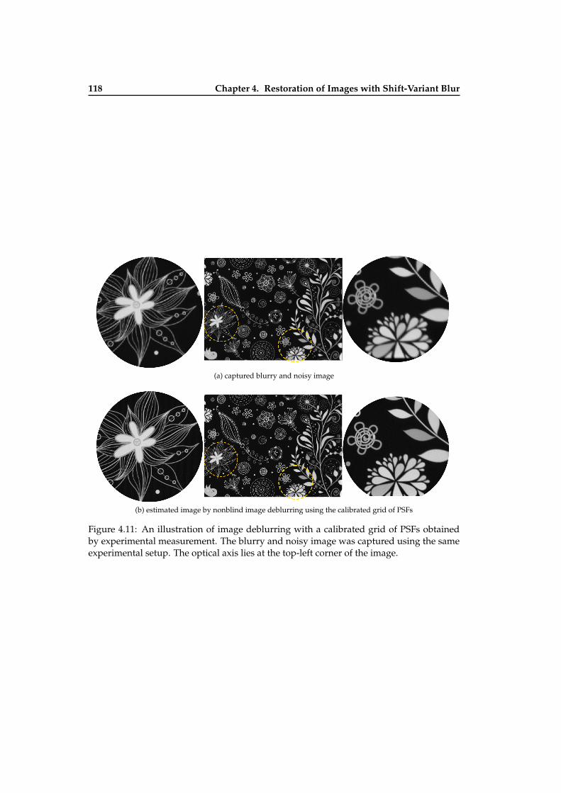
118 Chapter 4. Restoration of Images with Shift-Variant Blur
(a) captured blurry and noisy image
(b) estimated image by nonblind image deblurring using the calibrated grid of PSFs
Figure 4.11: An illustration of image deblurring with a calibrated grid of PSFs obtainedby experimental measurement. The blurry and noisy image was captured using the sameexperimental setup. The optical axis lies at the top-left corner of the image.
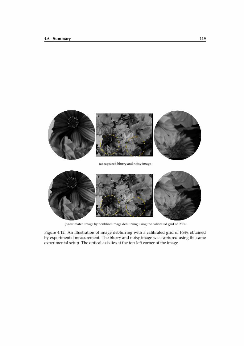
4.6. Summary 119
(a) captured blurry and noisy image
(b) estimated image by nonblind image deblurring using the calibrated grid of PSFs
Figure 4.12: An illustration of image deblurring with a calibrated grid of PSFs obtainedby experimental measurement. The blurry and noisy image was captured using the sameexperimental setup. The optical axis lies at the top-left corner of the image.

CHAPTER 5
Conclusions and Future Works
The future is not so far away, yet not so trivial to reach there...– Anonymous
5.1 Discussion and Conclusion
This thesis covers the subject of image deblurring. It starts with an overview of imagerestoration, with a special focus on shift-variant blur modeling. Image deblurring is statedas a large-scale numerical optimization problem, with non-smooth terms and/or con-straints. This calls for the development of a versatile optimization algorithm. The pro-posed optimization algorithm, ALBHO, is of practical interest due to its fast convergencewithout the hassle of tuning parameters. A blind image deblurring via image decomposi-tion, BDID, is proposed for restoration of astronomical scenes. The results obtained fromBDID are convincing, and the method is close to applicability in astronomical applications.Finally, the thesis presents a detailed discussion on image deblurring and PSFs estimationin case of shift-variant blur. It clearly shows the necessity of shift-variant image deblur-ring for many imaging situations, and proposes an approach to estimate PSFs from imagesdegraded by optical aberrations. The results from shift-variant PSFs estimation using a cal-ibrated camera, and then image deblurring using the estimated PSFs are convincing. Thenext step will be toward shift-variant blind image deblurring. In the following, I will putdiscussion, limitations and conclusion for each chapter of the thesis.
• In Chapter 1, we saw a general overview of imaging systems and image formationmodels for both shift-invariant and shift-variant blur. The chapter explains the fun-damental causes of blur and noise present in acquired images. It points out thenecessities of modeling blur in many imaging systems by a shift-variant blur model,and then it describes several approximations for shift-variant blur with their advan-tages and limitations. This chapter sheds light on different types of problems underthe general topic of image restoration, then it presents the Bayesian inference formu-lation for general image restoration problem, and discusses several special cases ofit. This chapter discusses different possible ways for solving the restoration prob-lem, in particular, it justifies the alternating minimization approach for blind imagerestoration over the hidden variable marginalization approach. The chapter ends witha detailed discussion on the ill-posedness of the restoration problem, and how tohandle it by using different types of prior/regularization in different situations.
• Throughout the thesis, a nonstationary white Gaussian noise model has been usedto approximate the mixture of Poisson and Gaussian noise present in images. Thisnoise model is pretty accurate for many imaging situations. An important topic thatshould be considered next is the accurate estimation of variance of noise present in
122 Chapter 5. Conclusions and Future Works
the images, which is very essential, and is related to the selection of regularizationparameters. The thesis does not discuss in detail how to select the hyperparame-ters/regularization parameters, which is very essential to obtain high quality imagefrom restoration technique. It is another difficult problem in image restoration. Lit-erature on regularization parameter selection is vast, so the near future task will beto adapt some existing methods with certain modifications/improvements for theimage restoration methods used or proposed in this thesis.
Few papers in literature, such as [Molina 2006, Babacan 2012], advocate to use hiddenvariable marginalization approach for blind image restoration in which all three un-known variables: the blur, the crisp image and the hyperparameters/regularizationparameters are estimated using the variable marginalization. However, in the litera-ture one would not find much works concerning the comparison of marginalizationapproach vs the alternating minimization with justifications for the cases where oneof them would perform better than the other. This could be an interesting futurelong-term work.
• Chapter 2 focuses on the optimization problems arising in imaging, computer visionand machine learning. The contribution of this chapter is to address a generic op-timization problem (constrained nonsmooth optimization problem) found in differ-ent domains, and the chapter proposes a class of optimization algorithms, ALBHO,for solving them. The proposed algorithms are based on variable splitting and theaugmented Lagrangian, and they are faster or at least as fast as the state-of-the-artalgorithms based on the augmented Lagrangian, while being hassle free of parame-ter tuning, which is a great relief for the users. Another advantage of this algorithmis its easy implementability with a part of its implementation comes from the wellestablished limited-memory quasi-Newton method with bound constraint, whichhave almost standard implementation in the literature. The chapters shows the ap-plicability of the proposed algorithm on different types of optimization problems.Since ALBHO is very general, it may be adapted for solving problems arising inother domains, such as machine learning. A short-term goal could be to compare itsefficiency to the state-of-the-art algorithms in machine learning.
• Chapter 3 discusses image decomposition approach for image restoration, which canbe seen as a way to design specific priors for structures in images. In particular, thechapter presents a blind image deblurring method via image decomposition for therestoration of astronomical images. The blind image restoration method is basedon the assumptions that astronomical images contain mainly two types of sources:point-like sources and extended smooth sources, and the blur is shift-invariant. Theproposed blind deblurring method, BDID, suggests to include several constraints toavoid the ill-posedness of the problem. The presented method solves the problemby alternating minimization, where the resulting subproblems (optimization problem)are efficiently solved by ALBHO proposed in Chapter 2. The restoration results ob-tained on synthetic astronomical images are promising. A near future work will beto improve it applicability to real astronomical applications, and validate the resultsusing astrometry and photometry.
• Chapter 4 deals with the restoration of images degraded by a shift-variant blur,which is relevant in many practical imaging situations, but is much harder than theclassical shift-invariant case. In many practical cases, the blur throughout the field ofview varies due to several reasons; considering a separate blurring operation at eachpixel location is computationally impractical. Thus, it becomes essential to model
5.2. Future Work 123
the shift-variant blur with an approximation, which can achieve a good trade-off be-tween the accuracy and the computational cost. Among the several existing approx-imation, this chapter advocates the use of the PSF interpolation approximation. Thischapter provides a detailed overview of this shift-variant approximation with its im-plementational aspects and the computational complexity. The main contributions ofthis chapter are the development of a shift-variant image deblurring, and the shift-variant PSFs estimation, which are the two steps towards blind image deblurring,the main long-term goal of this thesis topic. In PSF estimation approach, characteris-tics of the blur due to optical aberrations are exploited to reduce the ill-posedness ofthe problem, and the numerical results show that this contribution is helpful for de-blurring images suffering from optical aberrations or similar shift-variant blur. Thishas been experimentally validated by deblurring images from a calibrated camera,and the calibration method has been described in detail. Since the two steps to-wards shift-variant blind image deblurring are working well, a near future work isto perform blind deblurring of real scenes suffering from shift-variant blurs, e.g. anextension to the blind image deblurring method presented in Chapter 3.
5.2 Future Work
I have pointed out in the Discussion and Conclusion section, some of the interesting nearfuture and long-term works based on this thesis. Here, I will recollect them in the sequencefrom short-term to a long-term future works:
• Application of the blind image deblurring method, BDID, proposed in Chapter 3 forreal astronomical images, and validation of the method by evaluating the astrometryand photometry of the restored images.
• Extension of the BDID to the case of shift-variant blur, first on numerical simulations,and then on real astronomical images.
• Extension of the blind image deblurring method for restoring natural images blurreddue to motion blur mostly happening in photography and computer vision applica-tions.
• Application of the shift-variant blind image deblurring method for restoring 3D mi-croscopy images for biomedical applications.
• The result of the restoration is very much dependent upon the choice of the regular-ization parameters, thus finding/developing an efficient method for regularizationparameter selection is very important.
• Comparison between the alternating minimization and variable marginalization ap-proaches for blind image restoration with analysis on the advantages one of themethod over the other both from a theoretical and practical point of view.
• Modeling efficiently and accurately the shift-variant blur happening due to a shal-low depth of field, occlusion and relative motion between the foreground and back-ground objects could be addressed in the long-term work.

CHAPTER 6
Conclusion et travaux futurs
The future is not so far away, yet not so trivial to reach there...– Anonymous
6.1 Discussion et Conclusion
Cette thèse traite du sujet de la restauration d’images. Elle démarre par une présenta-tion générale de la restauration d’images, avec un focus particulier sur la modélisation duflou variable dans le champ. La restauration d’images est reformulée comme un problèmed’optimisation en grande dimension, avec des termes non lisses et/ou des contraintes. Elleest donc nécessaire de développer un algorithme d’optimisation générique. L’algorithmeproposé, ALBHO, est utile en pratique car il converge rapidement sans nécessiter de ré-gler de nombreux paramètres. Une méthode de déconvolution aveugle basée sur la dé-composition d’images en sources ponctuelles et sources étendues est proposée pour larestauration d’images astronomiques. Les résultats obtenus sont encourageants pour uneapplication, après adaptation, sur des jeux de données réelles. Enfin, la thèse présenteune discussion détaillée sur la restauration d’images et l’estimation du flou dans le cas deflous spatialement variables. Il met en évidence la nécessité de corriger le flou dans dif-férents contextes et propose une méthode pour l’étalonnage du flou. Les résultats expéri-mentaux d’estimation du flou, puis de restauration d’images floues valident les méthodesdéveloppées. Ces méthodes forment les briques de base pour attaquer le problème de larestauration aveugle d’images dégradées par un flou spatialement variable. Je détaille ci-dessous les contributions propres à chaque chapitre, les limitations et les perspectives deces travaux:
• Le chapitre 1 donne une présentation générale des systèmes d’imagerie et des mod-èles de formation de l’image dans le cas de flous invariants et spatialement variables.Les différentes causes du flou et du bruit présents dans les images sont analysées.L’importance de la modélisation des variations spatiales du flou est pointée et dif-férentes approximations du flou sont décrites ainsi que leurs avantages et limites.Le chapitre discute de différents types de problèmes rencontrés dans le cadre dela restauration d’images, puis présente une formulation générale de la restaurationd’images dans le cadre bayésien ainsi que ses différentes déclinaisons. Différentesfaçons de résoudre le problème de restauration sont envisagées et le choix d’une ap-proche de type minimisation alternée plutôt que marginalisation pour la restaurationaveugle est justifiée. Le chapitre se termine par une discussion de la difficulté duproblème de restauration et comment des stratégies de régularisation peuvent êtremises au point pour mieux contraindre le problème.
• Tout au long de la thèse, un modèle de bruit blanc gaussien non stationnaire est util-isé pour approximer le mélange de bruit gaussien et de bruit poissonnien présent

126 Chapter 6. Conclusion et travaux futurs
dans les images. Ce modèle de bruit est relativement précis dans de nombreux cas.Une question importante qui mérite une investigation est l’estimation de la vari-ance du bruit dans les images, un problème lié au problème du réglage des hyper-paramètres, c’est à dire des paramètres de régularisation des méthodes restauration.Le réglage de ces hyper-paramètres n’a pas été abordé dans cette thèse. Une largebibliographie existe sur le sujet. Une perspective à court terme consisterait à adapterces techniques aux méthodes de restauration proposées dans cette thèse.
Quelques travaux dans la littérature, tels [Molina 2006, Babacan 2012], proposentd’utiliser une approche de type marginalisation pour la restauration aveugle etl’estimation des hyper-paramètres. Il manque cependant une comparaison de cetteapproche avec la minimisation alternée que nous avons utilisée, avec une justificationdes cas dans lesquels l’une est préférable par rapport à l’autre. Cela pourrait être uneperspective intéressante.
• Le chapitre 2 se focalise sur les problèmes d’optimisation apparaissant en imagerie etque l’on rencontre également en vision par ordinateur ou en apprentissage automa-tique. La contribution de ce chapitre est une classe d’algorithmes d’optimisation,ALBHO, permettant de résoudre des problèmes d’optimisation généraux (de type“optimisation non-lisse sous contraintes”). Les algorithmes proposés sont basés surle principe de la séparation de variables et du lagrangien augmenté. Ils sont aussirapides, voire plus rapides que les méthodes de l’état de l’art également basées sur lelagrangien augmenté tout en étant beaucoup plus faciles d’utilisation car ne nécessi-tant pas le réglage de nombreux paramètres. Un autre avantage de ces algorithmesest leur implémentation facile, le cœur de l’algorithme étant constitué d’un algo-rithme d’optimisation de quasi-Newton à mémoire limitée, dont il existe des implé-mentations bien établies. Le chapitre illustre sur plusieurs problèmes d’optimisationl’application des algorithmes ALBHO. Puisqu’il s’agit d’une méthode générale, ellepeut être utile pour résoudre des problèmes d’optimisation rencontrés dans d’autresdomaines applicatifs comme l’apprentissage automatique. Des travaux futurs pour-raient porter sur la comparaison d’ALBHO aux méthodes état de l’art en apprentis-sage automatique.
• Le chapitre 3 présente une approche de décomposition d’images pour la restaura-tion. La décomposition d’une image en plusieurs composantes permet d’associer àchacune un a priori spécifique et modéliser ainsi la présence de structures plus com-plexes. Plus précisément, le chapitre décrit une méthode de déconvolution aveugledestinée aux images astronomiques dont l’étape de restauration est basée sur unedécomposition d’images. La décomposition est basée sur l’hypothèse que les im-ages astronomiques contiennent essentiellement deux types de sources: les sourcesponctuelles et les sources étendues. La méthode de restauration aveugle proposée,appliquée au cas des flous stationnaires, inclut plusieurs contraintes dans la procé-dure d’estimation. Le problème de déconvolution aveugle est résolu par minimi-sation alternée et chaque sous-problème d’optimisation est résolu par une instanced’ALBHO décrit au chapitre 2. Les résultats de restauration obtenus sur des imagessynthétiques sont encourageants. Les travaux futurs à court terme porteront surl’application à des données astronomiques réelles et sur la validation des résultatsen étudiant les précisions astrométriques et photométriques.
• Le chapitre 4 porte sur la restauration d’images dégradées par un flou variable dansle champ. De tels flous sont rencontrés dans divers contextes applicatifs mais leurestimation et leur inversion est plus difficile que pour les flous stationnaires. Il est en

6.2. Travaux futurs 127
effet nécessaire de trouver un compromis entre la flexibilité du modèle de flou afinpouvoir décrire précisément les différents cas rencontrés en pratique et le nombre dedegrés de libertés à résoudre lors de l’estimation. Ce chapitre utilise un modèle basésur l’interpolation d’une grille de réponses impulsionnelles. Après avoir détailléla complexité algorithmique de ce modèle et l’avoir appliqué sur une simulationnumérique dans laquelle le flou est supposé connu, le problème de l’estimation d’unflou spatialement variable est présenté. La méthode d’estimation du flou et la méth-ode de restauration forment les deux briques nécessaires à la réalisation à plus longterme de la restauration aveugle d’images dégradées par un flou non stationnaire.Lors de l’estimation du flou, les caractéristiques des aberrations optiques sont ex-ploitées afin de contraindre le problème d’estimation. Les expériences numériquesmontrent que ces contraintes permettent de reconstruire le flou. Ensuite, une val-idation expérimentale est conduite pour valider la méthode d’étalonnage du flouet pour évaluer l’apport de la restauration basée sur un modèle non stationnairedu flou. Puisque chacune des deux étapes nécessaires à la restauration aveugle aété validée, une perspective à court terme est de réaliser une restauration aveuglede scènes réelles, par exemple en étendant la méthode de déconvolution aveugleprésentée au chapitre 3.
6.2 Travaux futurs
J’ai pointé dans le paragraphe précédent un certain nombre de perspectives à court oumoyen terme pouvant faire suite à ces travaux de thèse. Je détaille ici ces perspectivesen les organisant depuis les perspectives à court terme jusqu’à celles qui relèvent d’uneréflexion à plus long terme:
• Application de la méthode de déconvolution aveugle du chapitre 3 à des jeux dedonnées astronomiques réelles, ainsi que validation de la méthode en évaluant lesprécisions astrométriques et photométriques dans les images restaurées.
• Extension de la méthode de déconvolution aveugle au cas du flou variable dansle champ, d’abord sur des simulations numériques, puis sur des données as-tronomiques réelles.
• Application de la méthode de restauration aveugle aux images naturelles dégradéespar un flou de bougé (applications en photographie et en vision par ordinateur).
• Application des algorithmes de restauration adaptés au cas de flous spatialementvariables aux images de microscopie 3D pour des applications biomédicales.
• Développement d’une méthode pour le réglage des paramètres de régularisation.
• Comparaison entre les stratégies de minimisation alternée et de marginalisation pourla restauration aveugle, avec analyse des avantages d’une méthode par rapport àl’autre à la fois d’un point de vue théorique et pratique.
• Modélisation et inversion du flou de défocalisation apparaissant dans les scènes 3D(notamment les occlusions) ainsi que lors du mouvement relatif d’objets pendant letemps d’intégration de la caméra.

APPENDIX A
Appendix
A.1 Functional Analysis
A.1.1 Definitions
• Open, Closed and Compact Sets: For a vector x ∈ Rn and a scalar ε > 0, let S(x; ε)
denotes an open sphere centered at xwith radius ε > 0, i.e.,
S(x; ε) = z|‖z − x‖2 < ε
A subset S ⊂ Rn is said to be open, if for every x ∈ S one can find an ε > 0 such thatS(x; ε) ⊂ S. If S is open and x ∈ S, then S is said to be a neighborhood of x.
A set S is closed if and only if its complement in Rn is open. Equivalently S is closedif and only if every convergent sequence xk with elements in S converges to a pointwhich also belongs to S .
A subset S of Rn is said to be compact if and only if it is both closed and bounded(i.e., it is closed and for some M > 0 we have ‖x‖2 ≤ M for all x ∈ S). A set S iscompact if and only if every sequence xk with elements in S has at least one limitpoint which belongs to S .
• Convex Sets: A set C ∈ Rn is convex if for any two points x,y ∈ C, the segmentjoining them belongs to C
αx+ (1− α)y ∈ C,∀α ∈ [0, 1]
• Continuous Function: A function f mapping a set S1 ⊂ Rn into a set S2 ⊂ Rmis denoted by f : S1 → S2. The function f is said to be continuous at x ∈ S1 iff(xk) → f(x) whenever xk → x. Equivalently f is continuous at x if given ε > 0
there is a δ > 0 such that ‖y − x‖2 < δ and y ∈ S1 implies ‖f(y)− f(x))‖2 < ε. Thefunction f is said to be continuous over S1 if it is continuous at every point x ∈ S1. IfS1,S2, and S3 are sets and f1 : S1 → S2 and f2 : S2 → S3 are functions, the functionf2 · f1 : S1 → S3 defined by (f1 · f2)(x) = f2[f2(x)] is called the composition of f1 andf2. If f1 : Rn → Rm and f2 : Rm → Rp are continuous, then f2 · f1 is also continuous.
• Differentiable Function: A real valued function f : X → R where X ⊂ Rn is said tobe continuously differentiable if the partial derivatives ∂f(x)/∂x1, · · · , ∂f(x/∂xn) ex-ist for each x ∈ X and are continuous function of x over X . This case is representedas f ∈ C1 over X . More generally f ∈ Cp over X for a function f : X → R, whereX ⊂ Rn is an open set if all partial derivatives of order p exist and are continuous asfunction of x over X .
• Convex Functions: Given a convex set C ⊆ Rn and a function f(x) : C → R; f is saidto be

130 Appendix A. Appendix
– convex on C if, ∀x,y ∈ C and α ∈ (0, 1),
f(αx+ (1− α)y) ≤ αf(x) + (1− α)f(y)
– strictly convex on C if the above inequality is strict
– strongly convex on C if ∀x,y ∈ C and α ∈ (0, 1), there exists a constant ε > 0
such that
f(αx+ (1− α)y) ≤ αf(x) + (1− α)f(y)− ε
2α(1− α)‖x− y‖22
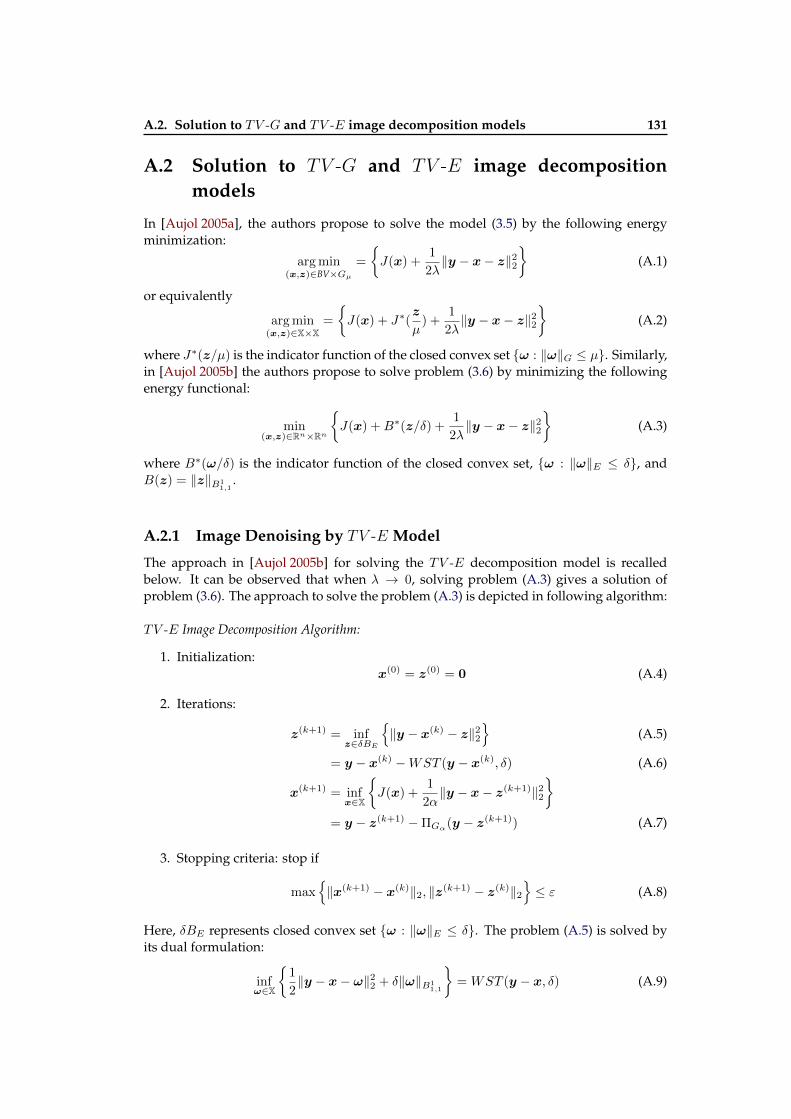
A.2. Solution to TV -G and TV -E image decomposition models 131
A.2 Solution to TV -G and TV -E image decompositionmodels
In [Aujol 2005a], the authors propose to solve the model (3.5) by the following energyminimization:
arg min(x,z)∈BV×Gµ
=
J(x) +
1
2λ‖y − x− z‖22
(A.1)
or equivalently
arg min(x,z)∈X×X
=
J(x) + J∗(
z
µ) +
1
2λ‖y − x− z‖22
(A.2)
where J∗(z/µ) is the indicator function of the closed convex set ω : ‖ω‖G ≤ µ. Similarly,in [Aujol 2005b] the authors propose to solve problem (3.6) by minimizing the followingenergy functional:
min(x,z)∈Rn×Rn
J(x) +B∗(z/δ) +
1
2λ‖y − x− z‖22
(A.3)
where B∗(ω/δ) is the indicator function of the closed convex set, ω : ‖ω‖E ≤ δ, andB(z) = ‖z‖B1
1,1.
A.2.1 Image Denoising by TV -E Model
The approach in [Aujol 2005b] for solving the TV -E decomposition model is recalledbelow. It can be observed that when λ → 0, solving problem (A.3) gives a solution ofproblem (3.6). The approach to solve the problem (A.3) is depicted in following algorithm:
TV -E Image Decomposition Algorithm:
1. Initialization:x(0) = z(0) = 0 (A.4)
2. Iterations:
z(k+1) = infz∈δBE
‖y − x(k) − z‖22
(A.5)
= y − x(k) −WST (y − x(k), δ) (A.6)
x(k+1) = infx∈X
J(x) +
1
2α‖y − x− z(k+1)‖22
= y − z(k+1) −ΠGα(y − z(k+1)) (A.7)
3. Stopping criteria: stop if
max‖x(k+1) − x(k)‖2, ‖z(k+1) − z(k)‖2
≤ ε (A.8)
Here, δBE represents closed convex set ω : ‖ω‖E ≤ δ. The problem (A.5) is solved byits dual formulation:
infω∈X
1
2‖y − x− ω‖22 + δ‖ω‖B1
1,1
= WST (y − x, δ) (A.9)

132 Appendix A. Appendix
which leads to the solution (A.6) (see Proposition 4.7 in [Aujol 2005b]), where WST de-notes wavelet soft-thresholding, and the threshold, δ, is estimated by δ = ησ
√2 log(n2),
and η ≤ 1. The ΠGα represents orthogonal projection on Gα, which can be computed byChambolle’s projection algorithm proposed in [Chambolle 2004].
In [Aujol 2005b], the authors shows that BV is well adapted for the geometrical partof an image, G for the texture part and E = B∞−1,∞ for the noise. They show by theirexperimental results that the model (3.6) is a very good candidate for denoising texturedimages. This can be due to the fact that it simultaneously minimizes the total variation ofrestored image and a Besov norm (which amounts to a wavelet shrinkage), thus benefitingfrom the advantages of both methods. However, better results are obtained by relativelyhigher computational cost than the TV -L2 model and wavelet soft-thresholding. The re-sults of my numerical experiments on Barbara and Lenna image, shown in Fig. A.1 andFig. A.2, also show that TV -E denoising model restores the textures better than TV-L2
denoising model and wavelet soft-thresholding (WST) method. The values of the regular-ization parameters α and η in the experiment are chosen in order to have possible best peaksignal-to-noise ratio (PSNR) and the MATLAB function “wpdencmp” used for computingthe wavelet denoising WST .
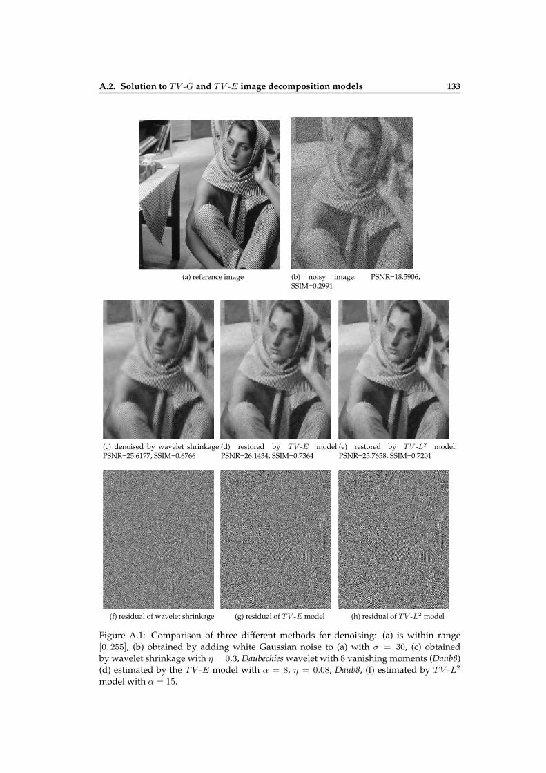
A.2. Solution to TV -G and TV -E image decomposition models 133
ref
50
100
150
200
(a) reference image
f with PSNR=18.5906; SSIM=0.2991
-50
0
50
100
150
200
250
300
(b) noisy image: PSNR=18.5906,SSIM=0.2991z with PSNR=25.6177; SSIM=0.6766
0
50
100
150
200
250
(c) denoised by wavelet shrinkage:PSNR=25.6177, SSIM=0.6766
u with PSNR=26.1434; SSIM=0.7364
0
50
100
150
200
250
(d) restored by TV -E model:PSNR=26.1434, SSIM=0.7364
y with PSNR=25.7658; SSIM=0.7201
50
100
150
200
(e) restored by TV -L2 model:PSNR=25.7658, SSIM=0.7201
f-z
-100
-50
0
50
100
(f) residual of wavelet shrinkage
f-u
-100
-80
-60
-40
-20
0
20
40
60
80
100
(g) residual of TV -E model
f-y
-80
-60
-40
-20
0
20
40
60
80
(h) residual of TV -L2 model
Figure A.1: Comparison of three different methods for denoising: (a) is within range[0, 255], (b) obtained by adding white Gaussian noise to (a) with σ = 30, (c) obtainedby wavelet shrinkage with η = 0.3, Daubechies wavelet with 8 vanishing moments (Daub8)(d) estimated by the TV -E model with α = 8, η = 0.08, Daub8, (f) estimated by TV -L2
model with α = 15.
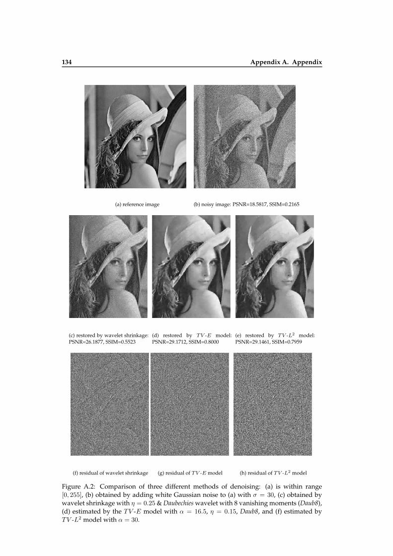
134 Appendix A. Appendix
ref
40
60
80
100
120
140
160
180
200
220
240
(a) reference image
f with PSNR=18.5817; SSIM=0.2165; MSE=4555.1772;
-50
0
50
100
150
200
250
300
(b) noisy image: PSNR=18.5817, SSIM=0.2165
z with PSNR=26.1877; SSIM=0.5523 MSE=6403.6394;
0
50
100
150
200
250
(c) restored by wavelet shrinkage:PSNR=26.1877, SSIM=0.5523
u with PSNR=29.1712; SSIM=0.8000 MSE=4542.0141;
20
40
60
80
100
120
140
160
180
200
220
(d) restored by TV -E model:PSNR=29.1712, SSIM=0.8000
y with PSNR=29.1461; SSIM=0.7959 MSE=4555.1772;
20
40
60
80
100
120
140
160
180
200
220
(e) restored by TV -L2 model:PSNR=29.1461, SSIM=0.7959
f-z
-100
-80
-60
-40
-20
0
20
40
60
80
100
(f) residual of wavelet shrinkage
f-u
-100
-50
0
50
100
(g) residual of TV -E model
f-y
-100
-80
-60
-40
-20
0
20
40
60
80
100
(h) residual of TV -L2 model
Figure A.2: Comparison of three different methods of denoising: (a) is within range[0, 255], (b) obtained by adding white Gaussian noise to (a) with σ = 30, (c) obtained bywavelet shrinkage with η = 0.25 & Daubechies wavelet with 8 vanishing moments (Daub8),(d) estimated by the TV -E model with α = 16.5, η = 0.15, Daub8, and (f) estimated byTV -L2 model with α = 30.

A.2. Solution to TV -G and TV -E image decomposition models 135
A.2.2 Image Deblurring via TV -E model
Seeing the performance of TV -E denoising model, in the Section A.2.1, in the restorationof the fine textures even in presence of heavy noise, here, I extend the TV -E decompositionmodel (A.3) for image deblurring purpose. The proposed TV -E deblurring model is basedon the following energy minimization:
arg min(0≤x, z)∈X2
J(x) +B∗(z/δ) +
1
2α‖y −Hx−Hz‖2W
(A.10)
where B∗(ω/δ) is indicator function of the closed convex set, ω : ‖ω‖E ≤ δ, y ∈ Xrepresents the available observed (blurred and noisy) image, x ∈ X represent the unknowntrue (original sharp) image, z ∈ X represents the fine texture parts, such as noise,H repre-sents the blurring operator (convolution matrix corresponding to a given PSF), and W isdiagonal weighing matrix, which has zero values, i.e., W i,i = 0 for unobserved i-th pixelvalues, for example unobservable pixels at the boundary of image sensor, and it has onesfor measured pixels, i.e.,W i,i = 1 for the observed ith pixel.
To minimize the above problem (A.10), a variable splitting and augmented Lagrangian(AL) approach is considered. With variable splittings: x = x, z = z, and ξ = y−Hx−Hz,, the augmented Lagrangian of the problem (A.10) is written as:
Lρ1,ρ2,ρ3(x, x, z, z, ξ,u1,u2,u3) = J(x) +ρ1
2‖x− x+ u1‖22
+B∗(z/δ) +ρ2
2‖z − z + u2‖22
+1
2α‖ξ‖2W +
ρ3
2‖y −Hx−Hz + u3‖22 (A.11)
where ρ1, ρ2, ρ3 > 0 are the augmented penalty parameters, and u1,u2,u3 ∈ X arescaled Lagrangian multipliers. It is possible to use ALBHO in Chapter 2 to find the saddlepoint of the AL (A.11) (the solution of problem (A.10) ), but I use a similar alternatingminimization approach as presented in Section A.2.1 in order that the deblurring resultsare not biased by the optimization method. The proposed algorithm for finding the saddlepoint of the augmented Lagrangian (A.11) is a variant of ADMM, and is as follows:
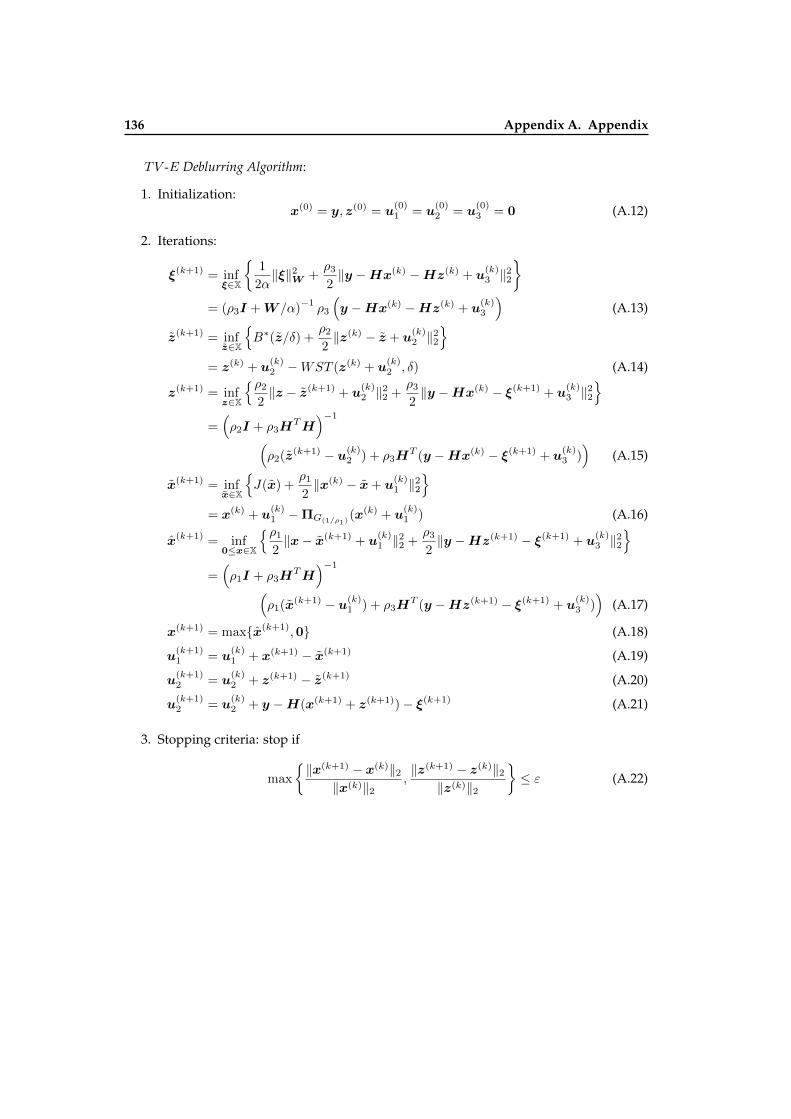
136 Appendix A. Appendix
TV -E Deblurring Algorithm:
1. Initialization:x(0) = y, z(0) = u
(0)1 = u
(0)2 = u
(0)3 = 0 (A.12)
2. Iterations:
ξ(k+1) = infξ∈X
1
2α‖ξ‖2W +
ρ3
2‖y −Hx(k) −Hz(k) + u
(k)3 ‖22
= (ρ3I +W /α)
−1ρ3
(y −Hx(k) −Hz(k) + u
(k)3
)(A.13)
z(k+1) = infz∈X
B∗(z/δ) +
ρ2
2‖z(k) − z + u
(k)2 ‖22
= z(k) + u
(k)2 −WST (z(k) + u
(k)2 , δ) (A.14)
z(k+1) = infz∈X
ρ2
2‖z − z(k+1) + u
(k)2 ‖22 +
ρ3
2‖y −Hx(k) − ξ(k+1) + u
(k)3 ‖22
=(ρ2I + ρ3H
TH)−1
(ρ2(z(k+1) − u(k)
2 ) + ρ3HT (y −Hx(k) − ξ(k+1) + u
(k)3 ))
(A.15)
x(k+1) = infx∈X
J(x) +
ρ1
2‖x(k) − x+ u
(k)1 ‖22
= x(k) + u
(k)1 −ΠG(1/ρ1)
(x(k) + u(k)1 ) (A.16)
x(k+1) = inf0≤x∈X
ρ1
2‖x− x(k+1) + u
(k)1 ‖22 +
ρ3
2‖y −Hz(k+1) − ξ(k+1) + u
(k)3 ‖22
=(ρ1I + ρ3H
TH)−1
(ρ1(x(k+1) − u(k)
1 ) + ρ3HT (y −Hz(k+1) − ξ(k+1) + u
(k)3 ))
(A.17)
x(k+1) = maxx(k+1),0 (A.18)
u(k+1)1 = u
(k)1 + x(k+1) − x(k+1) (A.19)
u(k+1)2 = u
(k)2 + z(k+1) − z(k+1) (A.20)
u(k+1)2 = u
(k)2 + y −H(x(k+1) + z(k+1))− ξ(k+1) (A.21)
3. Stopping criteria: stop if
max
‖x(k+1) − x(k)‖2‖x(k)‖2
,‖z(k+1) − z(k)‖2‖z(k)‖2
≤ ε (A.22)
A.2. Solution to TV -G and TV -E image decomposition models 137
Here again, WST represents the wavelet soft-thresholding, and the threshold is esti-mated as δ = ησ
√2 log(n2), and η ≤ 1. The ΠG(1/ρ1)
represents orthogonal projector onG(1/ρ1), which is computed by Chambolle’s projection algorithm [Chambolle 2004]. Thematrix-vector multiplications, such asHx andHTy can be computed efficiently in Fourierdomain using FFTs. Similarly, the matrix inversions in (A.15) and (A.17) can also com-puted efficiently in Fourier domain. The matrix inversion in (A.13) is straight forwardsinceW is diagonal. In my experiments, the augmented penalty parameters ρ1, ρ2, and ρ3
are chosen heuristically to have possible fast convergence. The regularization parametersα and η are also chosen to have possible high values of image quality metrics, PSNR.Conclusions: The results of TV -E deblurring model on natural images, illustrated in Fig.A.3 and Fig.A.4, clearly show that the TV -E deblurring model is able to restore the tex-tures in images better than TV -L2 deblurring model. Thus, one can expect to have a betterimage quality from blind image deblurring restoration using this TV -E or similar imagedecomposition model, e.g., the fine details in the smooth extended sources in astronomicalimage as illustrated in Fig. 3.11 can be enhanced.
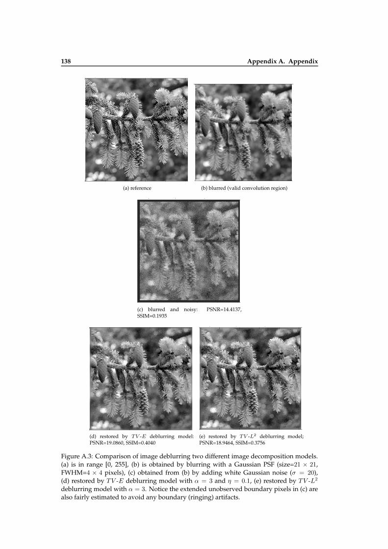
138 Appendix A. Appendixref:
MIN = 0.0000, MAX = 255.0000, MEAN = 116.0326, STD = 54.9250
0 100 200 300 400 500
50
100
150
200
250
300
350
400
450
5000
50
100
150
200
250
(a) reference
blurred image: MIN = 3.3715, MAX = 252.3056, MEAN = 115.7124, STD = 44.6069
0 100 200 300 400 500
50
100
150
200
250
300
350
400
450
50
100
150
200
250
(b) blurred (valid convolution region)f: PSNR = 14.4137 SSIM = 0.1935
MIN = -62.1775, MAX = 310.4161, MEAN = 106.8816, STD = 56.2036
0 100 200 300 400 500
50
100
150
200
250
300
350
400
450
500 -50
0
50
100
150
200
250
300
(c) blurred and noisy: PSNR=14.4137,SSIM=0.1935
u: PSNR = 19.0860 SSIM = 0.4040 MIN = 0.0000, MAX = 255.0000, MEAN = 115.9471, STD = 46.0462
0 100 200 300 400 500
50
100
150
200
250
300
350
400
450
5000
50
100
150
200
250
(d) restored by TV -E deblurring model:PSNR=19.0860, SSIM=0.4040
y: PSNR = 18.9464 SSIM = 0.3756 MIN = 0.0000, MAX = 255.0000, MEAN = 115.9081, STD = 46.7472
0 100 200 300 400 500
50
100
150
200
250
300
350
400
450
5000
50
100
150
200
250
(e) restored by TV -L2 deblurring model;PSNR=18.9464, SSIM=0.3756
Figure A.3: Comparison of image deblurring two different image decomposition models.(a) is in range [0, 255], (b) is obtained by blurring with a Gaussian PSF (size=21 × 21,FWHM=4 × 4 pixels), (c) obtained from (b) by adding white Gaussian noise (σ = 20),(d) restored by TV -E deblurring model with α = 3 and η = 0.1, (e) restored by TV -L2
deblurring model with α = 3. Notice the extended unobserved boundary pixels in (c) arealso fairly estimated to avoid any boundary (ringing) artifacts.

A.2. Solution to TV -G and TV -E image decomposition models 139ref:
MIN = 0.0000, MAX = 255.0000, MEAN = 101.7804, STD = 65.0349
0 100 200 300 400 500
50
100
150
200
250
300
350
400
450
5000
50
100
150
200
250
(a) reference
blurred image: MIN = 0.0727, MAX = 251.5084, MEAN = 102.2993, STD = 60.8280
0 100 200 300 400 500
50
100
150
200
250
300
350
400
450
50
100
150
200
250
(b) blurred (valid convolution region)f: PSNR = 16.8730 SSIM = 0.3776
MIN = -16.1358, MAX = 264.3562, MEAN = 94.4715, STD = 64.6549
0 100 200 300 400 500
50
100
150
200
250
300
350
400
450
5000
50
100
150
200
250
(c) blurred and noisy: PSNR=16.8730,SSIM=0.3776
u: PSNR = 23.8277 SSIM = 0.5510 MIN = 0.0000, MAX = 255.0000, MEAN = 101.4424, STD = 62.4734
0 100 200 300 400 500
50
100
150
200
250
300
350
400
450
5000
50
100
150
200
250
(d) restored by TV -E deblurring model:PSNR=23.8277, SSIM=0.5510
y: PSNR = 22.7353 SSIM = 0.5308 MIN = 0.0000, MAX = 255.0000, MEAN = 101.1389, STD = 62.7879
0 100 200 300 400 500
50
100
150
200
250
300
350
400
450
5000
50
100
150
200
250
(e) restored by TV -L2 deblurring model:PSNR=22.7353, SSIM=0.5308
Figure A.4: Comparison of image deblurring two different image decomposition models.(a) is in range [0, 255], (b) is obtained by blurring with a Gaussian PSF (size=21 × 21,FWHM=4 × 4 pixels), (c) obtained from (b) by adding white Gaussian noise (σ = 5), (d)restored by TV -E deblurring model with α = 0.6 and η = 0.05, (e) restored by TV -L2
deblurring model with α = 0.6. Notice the extended unobserved boundary pixels in (c)are also fairly estimated to avoid any boundary (ringing) artifacts.

Bibliography
[Afonso 2010a] Manya V Afonso, José M Bioucas-Dias and Mário a T Figueiredo. Fastimage recovery using variable splitting and constrained optimization. IEEE Trans. imageProcess., vol. 19, no. 9, pages 2345–2356, 2010. (Cited on pages 41 and 42.)
[Afonso 2010b] Manya V Afonso and A T Figueiredo. A fast algorithm for the constrained for-mulation of compressive image reconstruction and other linear inverse problems. In IEEEInternational Conference on Acoustics Speech and Signal Processing (ICASSP),numéro 3, pages 4034–4037. IEEE, 2010. (Cited on pages 41 and 42.)
[Afonso 2011] Manya V Afonso, José M Bioucas-dias and M. A. T. Figueiredo. An Aug-mented Lagrangian Approach to the Constrained Optimization Formulation of ImagingInverse Problems. IEEE Trans. Image Process., vol. 20, no. 3, pages 681–695, 2011.(Cited on pages 41 and 42.)
[Almeida 2010] M. S. C. Almeida and L. B. Almeida. Blind and Semi-Blind Deblurring ofNatural Images. IEEE Trans. on Image Processing, vol. 19, no. 1, pages 36–52, 2010.(Cited on pages 26 and 76.)
[Aujol 2003] Jean-François Aujol, Gilles Aubert, Laure Blanc-Féraud and Antonin Cham-bolle. Image Decomposition Application to SAR Images. In LewisD. Griffin and MartinLillholm, editeurs, Scale Sp. Methods Comput. Vis., volume 2695 of Lecture Notesin Computer Science, pages 297–312. Springer, 2003. (Cited on page 75.)
[Aujol 2005a] JF Aujol, G Aubert, Laure Blanc-Féraud and Antonin Chambolle. Imagedecomposition into a bounded variation component and an oscillating component. J. Math.Imaging Vis., vol. 22, no. 1, pages 71–88, 2005. (Cited on pages 73, 75 and 131.)
[Aujol 2005b] JF Aujol and Antonin Chambolle. Dual norms and image decomposition models.Int. J. Comput. Vis., vol. 63, no. 1, pages 85–104, 2005. (Cited on pages 73, 131and 132.)
[Aujol 2006] JF Aujol, Guy Gilboa, Tony Chan and Stanley Osher. Structure-texture im-age decomposition—modeling, algorithms, and parameter selection. Int. J. Comput. Vis.,vol. 67, no. 1, pages 111–136, 2006. (Cited on page 73.)
[Ayers 1988] G. R. Ayers and J. C. Dainty. Iterative blind deconvolution and its applications.Opt. Lett., vol. 13, pages 547–549, 1988. (Cited on pages 22 and 76.)
[Babacan 2012] S Derin Babacan, Rafael Molina and Minh N Do. Bayesian Blind Deconvo-lution with General Sparse Image Priors. In Eur. Conf. Comput. Vis., pages 341–355,2012. (Cited on pages 22, 23, 27, 122 and 126.)
[Bardsley 2006] Johnathan Bardsley, Stuart Jefferies, James Nagy and Robert Plemmons.A computational method for the restoration of images with an unknown, spatially-varyingblur. Optics express, vol. 14, no. 5, pages 1767–1782, 2006. (Cited on page 12.)
[Beck 2009a] Amir Beck and Marc Teboulle. A Fast Iterative Shrinkage-Thresholding Algo-rithm for Linear Inverse Problems. SIAM Journal of Imaging Sciences, vol. 2, no. 1,pages 183–202, 2009. (Cited on pages 41 and 42.)
142 Bibliography
[Beck 2009b] Amir Beck and Marc Teboulle. Fast gradient-based algorithms for constrainedtotal variation image denoising and deblurring problems. IEEE Trans. image Process.,vol. 18, no. 11, pages 2419–34, 2009. (Cited on pages 38, 41 and 42.)
[Beck 2010] Amir Beck and Marc Teboulle. Gradient-Based Algorithms with Applications toSignal Recovery Problems. In Daniel P. Palomar and Yonina C. Eldar, editeurs, Con-vex Optimization in Signal Processing and Communications, chapitre 2, pages 3–51. Cambridge University Press, New York, 1 édition, 2010. (Cited on page 37.)
[Becker 2011] Stephen Becker, Jerome Bobin and Emmanuel J. Candes. Nesta: a fast andaccurate first-order method for sparse recovery. SIAM J. Imaging Sci., vol. 4, no. 1,pages 1–39, 2011. (Cited on page 42.)
[Benson 2001] Steven J Benson and Jorge J Moré. A Limited Memory Variable MetricMethod in Subspaces and Bound Constrained Optimization Problems. Rapport tech-nique ANL/MCS-P909-0901, Math. and Computer Science Division, Argonne Na-tional Laboratory, 2001. (Cited on pages xvii, 36 and 44.)
[Bertsekas 1976] Dimitri P. Bertsekas. Multiplier methods: A survey. Automatica, vol. 12,no. 2, pages 133–145, 1976. (Cited on page 41.)
[Bertsekas 2004] Dimitri P. Bertsekas. Nonlinear programming. Athena, 2 édition, 2004.(Cited on pages 36, 38 and 39.)
[Bioucas-Dias 2007] José M. Bioucas-Dias and Mário A. T. Figueiredo. A New TwIST: Two-Step Iterative Shrinkage/Thresholding Algorithms for Image Restoration. IEEE Trans-actions on Image Processing, vol. 16, no. 12, pages 2992–3004, 2007. (Cited onpages 38 and 42.)
[Birgin 2000] Ernesto G. Birgin, José Mario Martínez and Marcos Raydan. NonmonotoneSpectral Projected Gradient Methods on Convex Sets. SIAM J. Numer. Anal., vol. 10,no. 4, pages 1196–1211, 2000. (Cited on pages 38 and 56.)
[Blanco ] L. Blanco and L. M. Mugnier. Marginal blind deconvolution of adaptive optics retinalimages. (Cited on page 22.)
[Boyd 2011] Stephen Boyd, Neal Parikh, Eric Chu, Borja Peleato and Jonathan Eckstein.Distributed Optimization and Statistical Learning via the Alternating Direction Methodof Multipliers. Journal of Foundations and Trends in Machine Learning, vol. 3, no. 1,pages 001–122, 2011. (Cited on pages 39 and 41.)
[Bresson 2007] Xavier Bresson, Selim Esedoglu, Pierre Vandergheynst, Jean-philippe Thi-ran and Stanley Osher. Fast Global Minimization of the Active Contour / Snake Model.J. Math. Imaging Vis., vol. 28, no. 2, pages 151–167, 2007. (Cited on page 52.)
[Bruck 1977] Ronald E. Bruck. On the Weak Convergence of an Ergodic Iteration for the So-lution of Variational Inequalities for Monotone Operators in Hilbert Space. Journal ofMathematical Analysis and Applications, vol. 61, pages 159–164, 1977. (Cited onpage 37.)
[Burke 2005] James V. Burke, Adrian S. Lewis and Michael L. Overton. A Robust Gradi-ent Sampling Algorithm for Nonsmooth, Nonconvex Optimization. SIAM Journal onOptimization, vol. 15, no. 3, pages 751–779, 2005. (Cited on page 37.)
Bibliography 143
[Calvetti 2000] Daniela Calvetti, Bryan Lewis and Lothar Reichel. Restoration of imageswith spatially variant blur by the GMRES method. In International Symposium onOptical Science and Technology, pages 364–374. International Society for Opticsand Photonics, 2000. (Cited on page 12.)
[Campisi 2007] Patrizio Campisi and Karen Egiazarian. Blind image deconvolution: the-ory and applications. CRC Press, 1 édition, 2007. (Cited on page 20.)
[Candes 1999] E. J. Candes and D. L. Donoho. Ridgelets: a key to higher-dimensional inter-mittency? Philos. Trans. R. Soc. A Math. Phys. Eng. Sci., vol. 357, no. 1760, pages2495–2509, 1999. (Cited on page 74.)
[Candès 2006] Emmanuel Candès, Laurent Demanet, David Donoho and Lexing Ying.Fast Discrete Curvelet Transforms. Multiscale Model. Simul., vol. 5, no. 3, pages 861–899, 2006. (Cited on page 74.)
[Cannon 1976] M. Cannon. Blind deconvolution of spatially invariant image blurs with phase.IEEE Trans. on Acoustics, Speech and Signal Processing, vol. 24, no. 1, pages 58 –63, 1976. (Cited on page 76.)
[Chacko 2013] Nikhil Chacko, Michael Liebling and Thierry Blu. Discretization of continu-ous convolution operators for accurate modeling of wave propagation in digital holography.JOSA A, vol. 30, no. 10, pages 2012–2020, 2013. (Cited on page 9.)
[Chambolle 2004] Antonin Chambolle. An algorithm for total variation minimization and ap-plications. J. Math. Imaging Vis., vol. 20, no. 1/2, pages 89–97, 2004. (Cited onpages 56, 132 and 137.)
[Chan 2000] T. F. Chan and C.K. Wong. Convergence of the alternating minimization algorithmfor blind deconvolution. Linear Algebra and its Applications, vol. 316, pages 259–285,2000. (Cited on pages 22 and 76.)
[Chan 2001] Tony F. Chan and Luminita a. Vese. Active contours without edges. IEEE Trans.Image Process., vol. 10, no. 2, pages 266–277, 2001. (Cited on page 52.)
[Chan 2006] Tony F. Chan, Selim Esedoglu and Mila Nikolova. Algorithms for finding globalminimizer of image segmentation and denoising models. SIAM J. Appl. Math., vol. 66,no. 5, pages 1632–1648, 2006. (Cited on page 52.)
[Chao 2006] Shin-Min Chao and Du-Ming Tsai. Astronomical image restoration using animproved anisotropic diffusion. Pattern Recognition Letters, vol. 27, no. 5, pages 335–344, 2006. (Cited on page 76.)
[Chouzenoux 2011] Emilie Chouzenoux, Jérôme Idier and Saïd Moussaoui. A Ma-jorize–Minimize Strategy for Subspace Optimization Applied to Image Restoration. IEEETranscations on Image Processing, vol. 20, no. 6, 2011. (Cited on page 36.)
[Chouzenoux 2013] Emilie Chouzenoux, Anna Jezierska, Jean-Christophe Pesquet andHugues Talbot. A Majorize-Minimize Subspace Approach for l2-l0 Image Regulariza-tion. SIAM Journal on Imaging Science, vol. 6, no. 1, 2013. (Cited on page 36.)
[Chouzenoux 2014] Emilie Chouzenoux, Jean-Christophe Pesquet and Audrey Repetti.Variable metric forward–backward algorithm for minimizing the sum of a differentiablefunction and a convex function. Journal of Optimization Theory and Applications,vol. 162, no. 1, pages 107–132, 2014. (Cited on page 39.)
144 Bibliography
[Chouzenoux 2015] Emilie Chouzenoux, Anna Jezierska, Jean-Christophe Pesquet andHugues Talbot. A Convex Approach for Image Restoration with Exact Poisson-GaussianLikelihood. Research report, LIGM, March 2015. (Cited on page 78.)
[Combettes 2005] Patrick L. Combettes and Valérie R. Wajs. Signal recovery by proximalforward-backward splitting. Multiscale Modeling & Simulation, vol. 4, no. 4, pages1168–1200, 2005. (Cited on page 37.)
[Combettes 2011] Patrick L Combettes and Jean-Christophe Pesquet. Proximal splittingmethods in signal processing. In Fixed-point algorithms for inverse problems in sci-ence and engineering, pages 185–212. Springer, 2011. (Cited on page 37.)
[Conan 2000] Jean-Marc Conan, Laurent M. Mugnier, Thierry Fusco, Vincent Michau andG\’erard Rousset. Myopic deconvolution of adaptive optics images by use of object andpoint-spread function power spectra: reply to comment. Applied Optics, vol. 39, pages2415–2417, 2000. (Cited on page 76.)
[Daubechies 2005] I. Daubechies and G. Teschke. Variational image restoration by means ofwavelets: Simultaneous decomposition, deblurring, and denoising. Applied and Com-putational Harmonic Analysis, vol. 19, no. 1, pages 1–16, 2005. (Cited on page 78.)
[Davidon 1991] William C. Davidon. Variable Metric Method for Minimization. SIAM Jour-nal of Optimization, vol. 1, no. 1, pages 1–17, 1991. (Cited on page 36.)
[Davies 2012] R. Davies and M. Kasper. Adaptive Optics for Astronomy. Annu. Rev. Astron.Astrophys., vol. 50, pages 305–351, 2012. (Cited on page 76.)
[Demanet 2007] Laurent Demanet and Lexing Ying. Wave Atoms and Sparsity of OscillatoryPatterns. Appl. Comput. Harmon. Anal., vol. 23, no. 3, pages 1–27, 2007. (Cited onpage 74.)
[Denis 2011] Loic Denis, Eric Thiebaut and Ferreol Soulez. Fast Model of Space-variant Blur-ring and its Application to Deconvolution in Astronomy. In Int. Conf. Image Process.,numéro 1, pages 2817 – 2820, Brussels, 2011. IEEE Xplore. (Cited on page 11.)
[Denis 2015] Loïc Denis, Eric Thiébaut, Ferréol Soulez, Jean-Marie Becker and RahulMourya. Fast Approximations of Shift-Variant Blur. International Journal of Com-puter Vision, pages 1–26, 2015. (Cited on pages 8, 9, 12, 13, 14, 15, 16 and 17.)
[Dennis 1977] J. E. Dennis and Jorge J. Moré. Quasi-Newton Methods, Motivation and Theory.SIAM Rev., vol. 19, no. 1, pages 46–89, 1977. (Cited on page 36.)
[Drummond 2009] Jack Drummond, Julian Christou, William J. Merline, Al Conrad andBenoit Carry. The Adaptive Optics Point Spread Function from Keck and Gemini. InAMOS Technical Conference, pages 1–9, Maui,Hawaii, 2009. AMOS. (Cited onpages 76, 79 and 83.)
[Eckstein 1992] Jonathan Eckstein and Dimitri P Bertsekas. On the Douglas-Rachford split-ting method and the proximal point algorithm for maximal monotone operators. Mathe-matical Programming, vol. 55, pages 293–318, 1992. (Cited on pages 41 and 52.)
[Elad 2007] Michael Elad, Peyman Milanfar and Ron Rubinstein. Analysis versus synthesisin signal priors. Inverse Problems, vol. 23, no. 3, pages 947–968, 2007. (Cited onpage 73.)

Bibliography 145
[Eldar 2009] Yonina C Eldar. Generalized SURE for exponential families: Applications to reg-ularization. Signal Processing, IEEE Transactions on, vol. 57, no. 2, pages 471–481,2009. (Cited on page 27.)
[Escande 2014] Paul Escande and Pierre Weiss. Numerical Computation of Spatially VaryingBlur Operators A Review of Existing Approaches with a New One. arXiv preprint, 2014.(Cited on page 11.)
[Fadili 2010] M Fadili, J Starck, J Bobin and Y Moudden. Image Decomposition and Sepa-ration Using Sparse Representations: An Overview. Proc. IEEE, vol. 98, no. 6, pages983–994, 2010. (Cited on page 73.)
[Fergus 2006] Rob Fergus, Barun Singh, Aaron Hertzmann, Sam T Roweis and William TFreeman. Removing Camera Shake from a Single Photograph. In ACM SIGGRAPH,SIGGRAPH ’06, pages 787–794, New York, NY, USA, 2006. ACM. (Cited onpages 22 and 26.)
[Figueiredo 2010] Mário a T Figueiredo and José M. Bioucas-Dias. Restoration of PoissonianImages Using Alternating Direction Optimization. IEEE Trans. Image Process., vol. 19,no. 12, pages 3549–3552, 2010. (Cited on pages 50, 51, 52 and 56.)
[Fletcher 1964] R. Fletcher and C. M. Reeves. Function minimization by conjugate gradients.The Computer Journal, vol. 7, no. 2, pages 149–154, 1964. (Cited on page 36.)
[Flicker 2005] Ralf C Flicker and François J Rigaut. Anisoplanatic deconvolution of adaptiveoptics images. JOSA A, vol. 22, no. 3, pages 504–513, 2005. (Cited on pages 12, 14and 17.)
[Foi 2008] Alessandro Foi, Mejdi Trimeche, Vladimir Katkovnik and Karen Egiazarian.Practical Poissonian-Gaussian noise modeling and fitting for single-image raw-data. IEEEtransactions on image processing : a publication of the IEEE Signal Processing So-ciety, vol. 17, no. 10, pages 1737–54, oct 2008. (Cited on page 24.)
[Fourier 1808] Joseph Fourier. Mémoire sur la propagation de la chaleur dans les corps solides.Nouveau Bulletin des Sciences de la Société Philomathique de Paris, vol. 6, pages112–116, 1808. (Cited on page 72.)
[Gabay 1976] D. Gabay and B. Mercier. A dual algorithm for the solution of nonlinear varia-tional problems via finite element approximations. Computers and Mathematics withApplications, vol. 2, pages 17–40, 1976. (Cited on page 39.)
[Gabay 1983] D. Gabay. Applications of the method of multipliers to variational inequalities. InAugmented Lagrangian Methods: Applications to the Solution of Boundary-ValueProblems, 1983. (Cited on page 41.)
[Galatsanos 1992] Nikolas P Galatsanos and Aggelos K Katsaggelos. Methods for choosingthe regularization parameter and estimating the noise variance in image restoration andtheir relation. Image Processing, IEEE Transactions on, vol. 1, no. 3, pages 322–336,1992. (Cited on page 27.)
[Gilad 2006] E. Gilad and J. Hardenberg. A fast algorithm for convolution integrals with spaceand time variant kernels. Journal of Computational Physics, vol. 216, no. 1, pages326–336, 2006. (Cited on pages 8 and 11.)
146 Bibliography
[Giovannelli 2005] J.-F. Giovannelli and A. Coulais. Positive deconvolution for superimposedextended source and point sources. Astron. Astrophys., vol. 439, no. 1, pages 401 – 412,2005. (Cited on page 78.)
[Giryes 2011] Raja Giryes, Michael Elad and Yonina C Eldar. The projected GSURE for au-tomatic parameter tuning in iterative shrinkage methods. Applied and ComputationalHarmonic Analysis, vol. 30, no. 3, pages 407–422, 2011. (Cited on page 27.)
[Goldstein 2010] Tom Goldstein, Xavier Bresson and Stanley Osher. Geometric Applicationsof the Split Bregman Method:Segmentation and Surface Reconstruction. J. Sci. Comput.,vol. 45, no. 1, pages 272–293, 2010. (Cited on pages xvii, 52, 53, 56 and 57.)
[Golub 1979] Gene H Golub, Michael Heath and Grace Wahba. Generalized cross-validationas a method for choosing a good ridge parameter. Technometrics, vol. 21, no. 2, pages215–223, 1979. (Cited on page 27.)
[Haarala 2004] M. Haarala, K. Miettinen and M.M. Mäkelä. New limited memory bundlemethod for large-scale nonsmooth optimization. Optimization Methods and Software,vol. 19, no. 6, pages 673–692, 2004. (Cited on page 37.)
[Hager 2006] William W. Hager and Hongchao Zhang. A New Active Set Algorithm forBox Constrained Optimization. SIAM Journal on Optimization, vol. 17, no. 2, pages526–557, 2006. (Cited on page 36.)
[Hansen 1993] Per Christian Hansen and Dianne Prost O’Leary. The use of the L-curve inthe regularization of discrete ill-posed problems. SIAM Journal on Scientific Computing,vol. 14, no. 6, pages 1487–1503, 1993. (Cited on page 27.)
[Harmeling 2009] S. Harmeling, M. Hirsch, S. Sra and B. Schölkopf. Online blind deconvo-lution for astronomical imaging. In IEEE Int. Conf. Comput. Photogr., pages 1–7, SanFrancisco, CA, 2009. (Cited on pages 76 and 97.)
[Hestenes 1952] Magnus R Hestenes and Eduard Stiefel. Methods of Conjugate Gradients forSolving Linear Systems. Journal of Research of the National Bureau of Standards,vol. 49, no. 6, pages 409–436, 1952. (Cited on page 36.)
[Hestenes 1969] M.R. Hestenes. Multiplier and Graidient Methods. Journal of OptmizationTheory and Applications, vol. 4, pages 303—-320, 1969. (Cited on page 40.)
[Hirsch 2010] Michael Hirsch, Suvrit Sra, Bernhard Sch, Stefan Harmeling and BiologicalCybernetics. Efficient Filter Flow for Space-Variant Multiframe Blind Deconvolution. InComputer Vision and Pattern Recognition, 2010. (Cited on pages 11, 14 and 17.)
[Hom 2007] Erik FY Hom, Franck Marchis, Timothy K Lee, Sebastian Haase, David AAgard and John W Sedat. AIDA: an adaptive image deconvolution algorithm withapplication to multi-frame and three-dimensional data. JOSA A, vol. 24, no. 6, pages1580–1600, 2007. (Cited on page 97.)
[Jefferies 1993] Stuart M. Jefferies and Julian C. Christou. Restoration of Astronomical Imagesby Iterative Blind Deconvolution. The Astrophysical Journal, vol. 415, page 862, 1993.(Cited on page 76.)
[Kahane 1995] Jean-Pierre Kahane, Pierre Gilles Lemarié and Pierre-Gilles Lemarié-Rieusset. Fourier series and wavelets, volume 3. Routledge, 1995. (Cited onpage 72.)
Bibliography 147
[Karmitsa 2010] Napsu Karmitsa and Marko M. Mäkelä. Limited memory bundle method forlarge bound constrained nonsmooth optimization: convergence analysis. OptimizationMethods and Software, vol. 25, no. 6, pages 895–916, 2010. (Cited on page 37.)
[Kass 2004] Michael Kass, Andrew Witkin and Demetri Terzopoulos. Snakes: Active con-tour models. Int. J. Comput. Vis., vol. 1, no. 4, pages 321–331, 2004. (Cited onpage 52.)
[Kiwiel 2007] Krzysztof C. Kiwiel. Convergence of the Gradient Sampling Algorithm for Nons-mooth Nonconvex Optimization. SIAM Journal on Optimization, vol. 18, no. 2, pages379–388, 2007. (Cited on page 37.)
[Kundur 1996] D. Kundur and D. Hatzinakos. Blind Image Deconvolution: A AlgorithmicApproach to Practical Image Restoration. IEEE Trans. Sig. Proc., vol. 13, no. 3, pages43–64, 1996. (Cited on page 22.)
[Lane 1992] R. G. Lane. Blind deconvolution of speckle images. J. Opt. Soc. Am. A, vol. 9,no. 9, pages 1508–1514, September 1992. (Cited on pages 76 and 80.)
[Lee 2014] Jason D Lee, Yuekai Sun and Michael A Saunders. Proximal newton-type methodsfor minimizing composite functions. SIAM Journal of Optimization, vol. 24, no. 3,pages 1420–1443, 2014. (Cited on pages xvii, 38, 39 and 42.)
[Lemaréchal 1982] Claude Lemaréchal. Numerical Experiments in Nonsmooth Optimization.In IIASA Workshop on Progress in Non-differentiable Optimization, pages 61–84,Laxenburg, Austria, 1982. (Cited on page 37.)
[Levin 2011a] A. Levin, Y. Weiss, F. Durand and W. T. Freeman. Understanding blind decon-volution algorithms. IEEE Trans. on Pattern Analysis Machine Intelligence, vol. 33,no. 12, pages 2354–2367, 2011. (Cited on pages 22, 23, 26 and 76.)
[Levin 2011b] Anat Levin, Yair Weiss, Fredo Durand and William T. Freeman. Efficientmarginal likelihood optimization in blind deconvolution. In Computer Vision and Pat-tern Recognition (CVPR), pages 2657–2664, Providence, RI, jun 2011. IEEE. (Citedon page 22.)
[Lewis 2012] Adrian S. Lewis and Michael L. Overton. Nonsmooth optimization via quasi-Newton methods. Mathematical Programming, vol. 141, no. 1, pages 135–163, 2012.(Cited on page 37.)
[Likas 2004] A.C. Likas and N. P Galatsanos. A Variational Approach for Bayesian BlindImage Deconvolution. IEEE Trans. on Signal Processing, vol. 52, no. 8, pages 2222–2233, 2004. (Cited on page 76.)
[Luksan 1999] L Luksan and J Vlcek. Globally Convergent Variable Metric Method for ConvexNonsmooth Unconstrained Minimization. Journal of Optimization Theory and Appli-cations, vol. 102, no. 3, pages 593–613, 1999. (Cited on page 37.)
[Maalouf 2011] Elie Maalouf, Bruno Colicchio and Alain Dieterlen. Fluorescence microscopythree-dimensional depth variant point spread function interpolation using Zernike mo-ments. JOSA A, vol. 28, no. 9, pages 1864–1870, 2011. (Cited on page 17.)
[Mallat 1993] Stéphane G Mallat and Zhifeng Zhang. Matching pursuits with time-frequencydictionaries. Signal Processing, IEEE Transactions on, vol. 41, no. 12, pages 3397–3415, 1993. (Cited on pages 72 and 74.)
148 Bibliography
[Mallat 1999] Stephane Mallat. A Wavelet Tour of Signal Processing. Elsevier, 2 édition,1999. (Cited on pages 72 and 74.)
[Matakos 2013] Antonios Matakos, Sathish Ramani and Jeffrey A. Fessler. AcceleratedEdge-Preserving Image Restoration Without Boundary Artifacts. IEEE Trans. ImageProcess., vol. 22, no. 5, pages 2019–2029, 2013. (Cited on pages 25, 41, 42, 47, 48, 50and 79.)
[Meyer 1997] François G. Meyer and Ronald R. Coifman. Brushlets: A Tool for DirectionalImage Analysis and Image Compression. Appl. Comput. Harmon. Anal., vol. 4, no. 2,pages 147–187, 1997. (Cited on page 74.)
[Meyer 2001] Yves Meyer. Oscillating patterns in image processing and nonlinear evolu-tion equations: The fifteenth dean jacqueline b. lewis memorial lectures. AmericanMathematical Society, Boston, MA, USA, 2001. (Cited on page 75.)
[Miraut 2012] David Miraut and Javier Portilla. Efficient shift-variant image restoration usingdeformable filtering (Part I). EURASIP J. Adv. Signal Process., vol. 2012, no. 1, page100, 2012. (Cited on page 12.)
[Miskin 2000] James Miskin and David JC MacKay. Ensemble learning for blind image sep-aration and deconvolution. In Advances in independent component analysis, pages123–141. Springer, 2000. (Cited on page 22.)
[Molina 1992] R Molina, Ascension del Olmo, Jaime Perea and BD Ripley. Bayesian de-convolution in optical astronomy. The Astronomical Journal, vol. 103, pages 666–675,1992. (Cited on page 76.)
[Molina 1994] Rafael Molina. On the Hierarchical Bayesian Approach to Image Restoration-Applications to Astronomical Images. IEEE Trans. Patt. Anal. Mach. Intell., vol. 16,no. 11, pages 1122–1128, 1994. (Cited on pages 20 and 22.)
[Molina 2001] R. Molina, J. Núñez and F. J. Cortijo. Image Restoration in Astronomy:ABayesian Perspective. IEEE Signal Processing Magazine, vol. 18, no. 2, pages 11–29,2001. (Cited on page 76.)
[Molina 2006] Rafael Molina, Javier Mateos and Aggelos K Katsaggelos. Blind deconvolu-tion using a variational approach to parameter, image, and blur estimation. IEEE Trans.image Process., vol. 15, no. 12, pages 3715–3727, 2006. (Cited on pages 22, 27, 76,122 and 126.)
[More 1994] J More and J Thuente. Line Search Algorithms with Guranteed Sufficient Decrease.ACM Transactions on Mathematical Software (TOMS), vol. 20, no. 3, pages 286–307, 1994. (Cited on pages 36 and 37.)
[Moreau 1965] J.-J. Moreau. Proximité et dualité dans un espace hilbertien. Bulletin de laSociété Mathématique de France, vol. 93, pages 273–299, 1965. (Cited on page 34.)
[Mourya 2015a] Rahul Mourya, Laboratoire Hubert Curien, Saint Etienne, Saint Genisand Laval Cedex. A Blind Deblurring and Image Decomposition Approach for Astro-nomical Image Restoration. In Eur. Signal Process. Conf., pages 1666–1670, Nice,France, 2015. IEEE. (Cited on page 76.)
Bibliography 149
[Mourya 2015b] Rahul Mourya, Loïc Denis, Eric Thiébaut and Jean-Marie Becker. Aug-mented Lagrangian Without Alternating Directions: Practical Algorithms for InverseProblems in Imaging. In IEEE International Conference on Image Processing, pages1–4, Quebec, Canada, 2015. (Cited on page 32.)
[Mugnier 2004] Laurent M Mugnier, Thierry Theirry Fusco and Jean-Marc Conan. MIS-TRAL: a myopic edge-perserving image restoration method, with application to astronomi-cal adaptive-optics-corrected long-exposure images. Journal of Optical Society of Amer-ica A, vol. 21, no. 10, pages 1841–1854, 2004. (Cited on pages 24, 76, 78 and 79.)
[Nagy 1998] James G Nagy and Dianne P. O’Leary. Restoring images degraded by spatiallyvariant blur*. SIAM J. Sci. Comput., vol. 19, no. 4, pages 1063–1082, 1998. (Cited onpages 12, 14 and 17.)
[Nagy 2004] James G Nagy, Katrina Palmer and Lisa Perrone. Iterative methods for imagedeblurring: a Matlab object-oriented approach. Numerical Algorithms, vol. 36, no. 1,pages 73–93, 2004. (Cited on page 12.)
[Nedic 2001] Angelia Nedic and Dimitri P Bertsekas. Convergence Rate of Incremental Sub-gradient Algorithms. Stochastic Optimization: Algorithms and Applications, vol. 54,pages 223–264, 2001. (Cited on page 37.)
[Nesterov 1983] Yurii Nesterov. A method for unconstrained convex minimization problem withthe rate of convergence O (1/k2). Doklady Akademii Nauk SSSR, vol. 269, no. 3, pages543–547, 1983. (Cited on page 38.)
[Nocedal 1980] Jorge Nocedal. Updating quasi-Newton matrices with limited storage. Math-ematics of computation, vol. 35, no. 151, pages 773–782, 1980. (Cited on pages 36,37 and 44.)
[Osher 2003] Stanley Osher, Andrés Solé and Luminita Vese. Image decomposition andrestoration using total variation minimization and the H 1. SIAM Multiscale Model.Simul., vol. 1, no. 3, pages 349–370, 2003. (Cited on pages 73 and 78.)
[Parikh 2013] Neal Parikh and Stephen Boyd. Proximal Algorithms. Foundations andTrends in Optimization, vol. 1, no. 3, pages 123–231, 2013. (Cited on page 34.)
[Passty 1979] Gregory B. Passty. Ergodic convergence to a zero of the sum of monotone operatorsin Hilbert space. Journal of Mathematical Analysis and Applications, vol. 72, no. 2,pages 383–390, 1979. (Cited on page 37.)
[Peyre 2007] Gabriel Peyre, Jalal Fadili and Jean-Luc Starck. Learning adapted dictionariesfor geometry and texture separation. In Proc. SPIE, Wavelets XII, volume 6701, pages67011T–67011T, 2007. (Cited on page 74.)
[Polak 1969] Elijah Polak and Gerard Ribiere. Note sur la convergence de méthodes de di-rections conjuguées. Revue française d’informatique et de recherche opérationnelle,série rouge, vol. 3, no. 1, pages 35–43, 1969. (Cited on page 36.)
[Porter 1984] Thomas Porter and Tom Duff. Compositing digital images. In ACM SiggraphComputer Graphics, volume 18, pages 253–259. ACM, 1984. (Cited on page 100.)
[Powell 1969] M.J.D. Powell. A method for nonlinear constraints in minimization prob-lems. Academic Press, New York, NY, 1969. (Cited on page 40.)
150 Bibliography
[Preza 2004] Chrysanthe Preza and José-Angel Conchello. Depth-variant maximum-likelihood restoration for three-dimensional fluorescence microscopy. JOSA A, vol. 21,no. 9, pages 1593–1601, 2004. (Cited on page 12.)
[Ramani 2008] Sathish Ramani, Thierry Blu and Michael Unser. Monte-Carlo SURE: Ablack-box optimization of regularization parameters for general denoising algorithms. Im-age Processing, IEEE Transactions on, vol. 17, no. 9, pages 1540–1554, 2008. (Citedon page 27.)
[Rigaut 2000] F. J. Rigaut, B. L. Ellerbroek and R. Flicker. Principles, limitations, and per-formance of multiconjugate adaptive optics. In Astronomical Telescopes and Instru-mentation, pages 1022–1031. International Society for Optics and Photonics, 2000.(Cited on page 76.)
[Rogers 2011] Adam Rogers and Jason D Fiege. Strong gravitational lens modeling withspatially variant point-spread functions. The Astrophysical Journal, vol. 743, no. 1,page 68, 2011. (Cited on page 12.)
[Rudin 1992] L Rudin, S Osher and E Fatemi. Nonlinear total variation based noise removalalgorithms. Phys. D Nonlinear Phenom., vol. 60, pages 259–268, 1992. (Cited onpages 26 and 74.)
[Schmidt 2009] Mark W Schmidt, Ewout van den Berg, Michael P. Friedlander and KevinMurphy. Optimizing costly functions with simple constraints: A limited-memory pro-jected quasi-newton algorithm. In International Conference on Artificial Intelligenceand Statistics, Clearwater Beach, Florida, April 2009. (Cited on pages 36 and 41.)
[Schmidt 2012] Mark Schmidt, Dongmin Kim and Suvrit Sra. Projected Newton-type Meth-ods in Machine Learning. Optimization for Machine Learning, pages 305–330, 2012.(Cited on pages xvii, 38, 39, 41 and 53.)
[Schuler 2012] Christian J Schuler, Michael Hirsch and Stefan Harmeling. Blind Correctionof Optical Aberrations. In European Conference on Computer Vision (ECCV), pages187–200, Florence, Italy, 2012. (Cited on page 108.)
[Schulz 1993] Timothy J Schulz. Multiframe blind deconvolution of astronomical images. JOSAA, vol. 10, no. 5, pages 1064–1073, 1993. (Cited on page 97.)
[Schulz 1997] T Schulz, B Stribling and J Miller. Multiframe blind deconvolution with realdata: imagery of the Hubble Space Telescope. Optics express, vol. 1, no. 11, pages 355–62, 1997. (Cited on page 76.)
[Starck 2005a] J-L Starck, Y Moudden, J Bobin, M Elad and DL Donoho. Morphological com-ponent analysis. In Optics & Photonics 2005, pages 59140Q–59140Q. InternationalSociety for Optics and Photonics, 2005. (Cited on pages 73 and 74.)
[Starck 2005b] Jean-Luc Starck, Michael Elad and David L Donoho. Image decomposition viathe combination of sparse representations and a variational approach. IEEE Trans. imageProcess., vol. 14, no. 10, pages 1570–82, oct 2005. (Cited on pages 73 and 78.)
[Stein 1981] Charles M Stein. Estimation of the mean of a multivariate normal distribution. Theannals of Statistics, pages 1135–1151, 1981. (Cited on page 27.)
[Teo 2010] Choon Hui Teo, S V N Vishwanathan, Alex Smola and Quoc V Le. BundleMethods for Regularized Risk Minimization. Journal of Machine Learning Research,vol. 11, pages 311–365, 2010. (Cited on page 37.)
Bibliography 151
[Thiébaut 2002] Éric Thiébaut. Optimization issues in blind deconvolution algorithms. In Proc.SPIE 4847, Astronomical Data Analysis II, Waikoloa, Hawaii, 2002. SPIE. (Cited onpages xvii, 22, 36, 44, 76 and 80.)
[Thiébaut 1995] É. Thiébaut and J.-M. Conan. Strict a priori constraints for maximum likeli-hood blind deconvolution. JOSAA, vol. 12, no. 3, pages 485–492, March 1995. (Citedon page 76.)
[Tseng 1991] Paul Tseng. Applications of a Splitting Algorithm to Decomposition in Convex Pro-gramming and Variational Inequalities. SIAM J. on Control and Optimization, vol. 29,no. 1, pages 119–138, 1991. (Cited on page 39.)
[Tsumuraya 1994] F Tsumuraya, N Miura and N Baba. Iterative blind deconvolution methodusing Lucy’s algorithm. Astronomy and Astrophysics, vol. 282, pages 699–708, 1994.(Cited on page 76.)
[Vese 2003] Luminita A Vese and Stanley J Osher. Modeling textures with total variation min-imization and oscillating patterns in image processing. Journal of Scientific Computing,vol. 19, no. 1-3, pages 553–572, 2003. (Cited on pages 73 and 75.)
[Wahba 1990] Grace Wahba. Spline models for observational data, volume 59. SIAM,1990. (Cited on page 27.)
[Wang 2008] Jue Wang and Michael F Cohen. Image and video matting: a survey. NowPublishers Inc, 2008. (Cited on page 100.)
[Wang 2013] Weiran Wang and Miguel Á. Carreira-Perpiñán. Projection onto the prob-ability simplex: An efficient algorithm with a simple proof, and an application.arXiv:1309.1541v1 [cs.LG], vol. abs/1309.1541, 2013. (Cited on pages 82 and 110.)
[Wang 2015] Wei Wang, Xile Zhao and Michael Ng. A cartoon-plus-texture image decomposi-tion model for blind deconvolution. Multidimensional Systems and Signal Processing,pages 1–22, 2015. (Cited on page 78.)
[Wipf 2014] David Wipf and Haichao Zhang. Revisiting Bayesian blind deconvolution. TheJournal of Machine Learning Research, vol. 15, no. 1, pages 3595–3634, 2014. (Citedon pages 23 and 77.)
[Xu 2013] Li Xu, Shicheng Zheng and Jiaya Jia. Unnatural L0 Sparse Representation for Nat-ural Image Deblurring. In IEEE Conference on Computer Vision and Pattern Recog-nition, pages 1107–1114. IEEE, 2013. (Cited on page 26.)
[You 1996] Yu-li You and M Kaveh. A Regularization Approach to Joint Blur Identificationand Image Restoration. IEEE Transaction on Image Processing, vol. 5, no. 3, pages416–428, 1996. (Cited on page 22.)
[Yu 2010] Jin Yu, S V N Vishwanathan and Nicol N Schraudolph. A Quasi-Newton Approachto Nonsmooth Convex Optimization Problems in Machine Learning. Journal of MachineLearning Research, vol. 11, pages 1145–1200, 2010. (Cited on page 37.)
[Zhu 1995] Ciyou Zhu, Richard Byrd, Jorge Nocedal and Jose Luis Morales. A LimitedMemory Algorithm for Bound Constrained Optimization. SIAM Journal on Scientificand Statistical Computing, vol. 16, no. 5, pages 1190–1208, 1995. (Cited on page 36.)

152 Bibliography
[Zibulevsky 2001] Michael Zibulevsky, Barak Pearlmutteret al. Blind source separation bysparse decomposition in a signal dictionary. Neural computation, vol. 13, no. 4, pages863–882, 2001. (Cited on page 73.)