Sensitivity and fragmentation calibration of the ROSINA ...
155
Sensitivity and fragmentation calibration of the ROSINA Double Focusing Mass Spectrometer Inauguraldissertation der Philosophisch-naturwissenschaftlichen Fakultät der Universität Bern vorgelegt von Myrtha Marianne Hässig von Krummenau SG Leiterin der Arbeit: Prof. Dr. Kathrin Altwegg Physikalisches Institut der Universität Bern Originaldokument gespeichert auf dem Webserver der Universitätsbibliothek Bern Dieses Werk ist unter einem Creative Commons Namensnennung-Keine kommerzielle Nutzung-Keine Bearbeitung 2.5 Schweiz Lizenzvertrag lizenziert. Um die Lizenz anzusehen, gehen Sie bitte zu http://creativecommons.org/licenses/by-nc-nd/2.5/ch/ oder schicken Sie einen Brief an Creative Commons, 171 Second Street, Suite 300, San Francisco, California 94105, USA.
-
Upload
khangminh22 -
Category
Documents
-
view
1 -
download
0
Transcript of Sensitivity and fragmentation calibration of the ROSINA ...

Sensitivity and fragmentation calibration of theROSINA Double Focusing Mass Spectrometer
Inauguraldissertation
der Philosophisch-naturwissenschaftlichen Fakultät
der Universität Bern
vorgelegt von
Myrtha Marianne Hässig
von Krummenau SG
Leiterin der Arbeit:
Prof. Dr. Kathrin Altwegg
Physikalisches Institut der Universität Bern
Originaldokument gespeichert auf dem Webserver der Universitätsbibliothek Bern
Dieses Werk ist unter einem
Creative Commons Namensnennung-Keine kommerzielle Nutzung-Keine Bearbeitung 2.5 Schweiz Lizenzvertrag lizenziert. Um die Lizenz anzusehen, gehen Sie bitte zu
http://creativecommons.org/licenses/by-nc-nd/2.5/ch/ oder schicken Sie einen Brief an Creative Commons, 171 Second Street, Suite 300, San Francisco, California 94105, USA.

Urheberrechtlicher Hinweis
Dieses Dokument steht unter einer Lizenz der Creative Commons Namensnennung-Keine kommerzielle Nutzung-Keine Bearbeitung 2.5 Schweiz.
http://creativecommons.org/licenses/by-nc-nd/2.5/ch/ Sie dürfen:
dieses Werk vervielfältigen, verbreiten und öffentlich zugänglich machen Zu den folgenden Bedingungen:
Namensnennung. Sie müssen den Namen des Autors/Rechteinhabers in der von ihm festgelegten Weise nennen (wodurch aber nicht der Eindruck entstehen darf, Sie oder die Nutzung des Werkes durch Sie würden entlohnt).
Keine kommerzielle Nutzung. Dieses Werk darf nicht für kommerzielle Zwecke verwendet werden.
Keine Bearbeitung. Dieses Werk darf nicht bearbeitet oder in anderer Weise verändert werden. Im Falle einer Verbreitung müssen Sie anderen die Lizenzbedingungen, unter welche dieses Werk fällt, mitteilen. Jede der vorgenannten Bedingungen kann aufgehoben werden, sofern Sie die Einwilligung des Rechteinhabers dazu erhalten. Diese Lizenz lässt die Urheberpersönlichkeitsrechte nach Schweizer Recht unberührt. Eine ausführliche Fassung des Lizenzvertrags befindet sich unter http://creativecommons.org/licenses/by-nc-nd/2.5/ch/legalcode.de

Sensitivity and fragmentation calibration of theROSINA Double Focusing Mass Spectrometer
Inauguraldissertation
der Philosophisch-naturwissenschaftlichen Fakultät
der Universität Bern
vorgelegt von
Myrtha Marianne Hässig
von Krummenau SG
Leiter/in der Arbeit:
Prof. Dr. Kathrin Altwegg
Physikalisches Institut der Universität Bern
Von der Philisophisch-naturwissenschaftlichen Fakultät angenommen.
Der Dekan:
Bern, den 06.09.2013 Prof. Dr. S. Decurtins


Abstract
The goal of this work has been to calibrate sensitivities and fragmentation pattern ofvarious molecules as well as further characterize the lab model of the ROSINA DoubleFocusing Mass Spectrometer (DFMS) on board ESA’s Rosetta spacecraft bound tocomet 67P/Churyumov-Gerasimenko. The detailed calibration and characterization ofthe instrument is key to understand and interpret the results in the coma of the comet.A static calibration was performed for the following species: Ne, Ar, Kr, Xe, H2O,N2, CO2, CH4, C2H6, C3H8, C4H10, and C2H4. The purpose of the calibration wasto obtain sensitivities for all detectors and emissions, the fragmentation behavior of theion source and to show the capabilities to measure isotopic ratios at the comet. Thecalibration included the recording of different correction factors to evaluate the data,including a detailed investigation of the detector gain. The quality of the calibrationthat could be tested for different gas mixtures including the calibration of the densityinside the ion source when calibration gas from the gas calibration unit is introduced.In conclusion the calibration shows that DFMS meets the design requirements and thatDFMS will be able to measure the D/H at the comet and help shed more light on thepuzzle about the origin of water on Earth.
Last compiled: 12.08.2013


CONTENTS
Contents
List of Tables iv
List of Figures vi
1 Introduction 1
2 Rosetta 52.1 The Mission . . . . . . . . . . . . . . . . . . . . . . . . . . . . . . . . . . . . . 52.2 67P/Churyumov-Gerasimenko . . . . . . . . . . . . . . . . . . . . . . . . . . . 7
2.2.1 Trajectories . . . . . . . . . . . . . . . . . . . . . . . . . . . . . . . . . 82.2.2 Cumulative flux for different trajectories . . . . . . . . . . . . . . . . . 11
2.3 Payload . . . . . . . . . . . . . . . . . . . . . . . . . . . . . . . . . . . . . . . 142.4 ROSINA . . . . . . . . . . . . . . . . . . . . . . . . . . . . . . . . . . . . . . . 15
2.4.1 COPS . . . . . . . . . . . . . . . . . . . . . . . . . . . . . . . . . . . . 162.4.2 RTOF . . . . . . . . . . . . . . . . . . . . . . . . . . . . . . . . . . . . 172.4.3 DFMS . . . . . . . . . . . . . . . . . . . . . . . . . . . . . . . . . . . . 172.4.4 DPU . . . . . . . . . . . . . . . . . . . . . . . . . . . . . . . . . . . . . 17
3 DFMS instrument description 193.1 Ion source . . . . . . . . . . . . . . . . . . . . . . . . . . . . . . . . . . . . . . 203.2 Transfer optics . . . . . . . . . . . . . . . . . . . . . . . . . . . . . . . . . . . 233.3 Electrostatic analyzer (ESA) . . . . . . . . . . . . . . . . . . . . . . . . . . . . 233.4 Magnet . . . . . . . . . . . . . . . . . . . . . . . . . . . . . . . . . . . . . . . 243.5 Zoom optics . . . . . . . . . . . . . . . . . . . . . . . . . . . . . . . . . . . . . 253.6 Detector package . . . . . . . . . . . . . . . . . . . . . . . . . . . . . . . . . . 25
3.6.1 MCP/LEDA . . . . . . . . . . . . . . . . . . . . . . . . . . . . . . . . 253.6.2 CEM . . . . . . . . . . . . . . . . . . . . . . . . . . . . . . . . . . . . . 273.6.3 FC . . . . . . . . . . . . . . . . . . . . . . . . . . . . . . . . . . . . . . 28
3.7 GCU . . . . . . . . . . . . . . . . . . . . . . . . . . . . . . . . . . . . . . . . . 283.8 DFMS operation . . . . . . . . . . . . . . . . . . . . . . . . . . . . . . . . . . 293.9 Technical problems . . . . . . . . . . . . . . . . . . . . . . . . . . . . . . . . . 30
4 DFMS characteristics 334.1 Ion source . . . . . . . . . . . . . . . . . . . . . . . . . . . . . . . . . . . . . . 33
4.1.1 Ionization cross section . . . . . . . . . . . . . . . . . . . . . . . . . . . 334.1.2 Fragmentation pattern . . . . . . . . . . . . . . . . . . . . . . . . . . . 34
4.2 Sensor transmission . . . . . . . . . . . . . . . . . . . . . . . . . . . . . . . . . 354.3 MCP/LEDA data . . . . . . . . . . . . . . . . . . . . . . . . . . . . . . . . . . 37
4.3.1 Offset correction . . . . . . . . . . . . . . . . . . . . . . . . . . . . . . 374.3.2 Individual pixel gain . . . . . . . . . . . . . . . . . . . . . . . . . . . . 384.3.3 Applying the mass scale . . . . . . . . . . . . . . . . . . . . . . . . . . 424.3.4 MCP/LEDA gain polynomial . . . . . . . . . . . . . . . . . . . . . . . 43
4.4 CEM data . . . . . . . . . . . . . . . . . . . . . . . . . . . . . . . . . . . . . . 464.5 FC data . . . . . . . . . . . . . . . . . . . . . . . . . . . . . . . . . . . . . . . 464.6 Sensitivity . . . . . . . . . . . . . . . . . . . . . . . . . . . . . . . . . . . . . . 47
i/ix

CONTENTS
5 Calibration of DFMS in a static environment 495.1 Calibration facility (CASYMIR) . . . . . . . . . . . . . . . . . . . . . . . . . . 495.2 Measurement procedure . . . . . . . . . . . . . . . . . . . . . . . . . . . . . . 515.3 Data treatment . . . . . . . . . . . . . . . . . . . . . . . . . . . . . . . . . . . 515.4 Noble Gases . . . . . . . . . . . . . . . . . . . . . . . . . . . . . . . . . . . . . 52
5.4.1 Ne Neon . . . . . . . . . . . . . . . . . . . . . . . . . . . . . . . . . . 535.4.2 Ar Argon . . . . . . . . . . . . . . . . . . . . . . . . . . . . . . . . . . 555.4.3 Kr Krypton . . . . . . . . . . . . . . . . . . . . . . . . . . . . . . . . . 575.4.4 Xe Xenon . . . . . . . . . . . . . . . . . . . . . . . . . . . . . . . . . . 60
5.5 H2O Water . . . . . . . . . . . . . . . . . . . . . . . . . . . . . . . . . . . . . 635.6 N2 Nitrogen . . . . . . . . . . . . . . . . . . . . . . . . . . . . . . . . . . . . . 685.7 CO2 Carbon dioxide . . . . . . . . . . . . . . . . . . . . . . . . . . . . . . . . 705.8 Alkanes . . . . . . . . . . . . . . . . . . . . . . . . . . . . . . . . . . . . . . . 73
5.8.1 CH4 Methane . . . . . . . . . . . . . . . . . . . . . . . . . . . . . . . . 735.8.2 C2H6 Ethane . . . . . . . . . . . . . . . . . . . . . . . . . . . . . . . . 765.8.3 C3H8 Propane . . . . . . . . . . . . . . . . . . . . . . . . . . . . . . . 795.8.4 C4H10 Butane . . . . . . . . . . . . . . . . . . . . . . . . . . . . . . . 82
5.9 Alkene . . . . . . . . . . . . . . . . . . . . . . . . . . . . . . . . . . . . . . . . 845.9.1 C2H4 Ethylene . . . . . . . . . . . . . . . . . . . . . . . . . . . . . . . 84
5.10 Minimal densities detectable with DFMS FM and adapted for FS . . . . . . . 87
6 Analysis of gas mixture 896.1 Data treatment . . . . . . . . . . . . . . . . . . . . . . . . . . . . . . . . . . . 896.2 Possible approach . . . . . . . . . . . . . . . . . . . . . . . . . . . . . . . . . . 906.3 GCU gas: Ne+CO2+Xe . . . . . . . . . . . . . . . . . . . . . . . . . . . . . . 906.4 Noble gas mixture: Ne–Ar–Kr–Xe . . . . . . . . . . . . . . . . . . . . . . . . 936.5 CO2+C3H8 . . . . . . . . . . . . . . . . . . . . . . . . . . . . . . . . . . . . . 96
7 Conclusion and outlook 101
Appendix 105
A SPICE Solar Aspect Angle (SAA) 106
B SPICE: Trajectories 111
C MCP gain calibration data 114
D Recorder files of the calibration 116
E Fragmentation pattern for MCP/LEDA and CEM (fi) and possible yieldcorrections 118
F Pressure correction factor for pressure sensor 126
G ROSINA/DFMS capabilities to measure isotopic ratios in water at comet67P/Churyumov-Gerasimenko 127
References 133
ii/ix

CONTENTS
Acknowledgments 139
Erklärung 141
Curriculum Vitae 143
iii/ix

LIST OF TABLES
List of Tables
1 Milestones of the Rosetta mission. . . . . . . . . . . . . . . . . . . . . . . . . 62 Orbital and physical characteristics of 67P/Churyumov-Gerasimenko [Lamy
et al., 2009] . . . . . . . . . . . . . . . . . . . . . . . . . . . . . . . . . . . . . 83 Total production rates for a low (LAC) and a high (HAC) active comet rep-
resenting possible scenarios for 67P/Churyumov-Gerasimenko at different he-liocentric distances. . . . . . . . . . . . . . . . . . . . . . . . . . . . . . . . . . 12
4 Rosetta Payload. Detailed description for every instrument can be found inthe Rosetta book Schulz et al. (2009) . . . . . . . . . . . . . . . . . . . . . . . 14
5 Ion source potentials of DFMS . . . . . . . . . . . . . . . . . . . . . . . . . . 216 Filament potentials of DFMS for filament 1 as emitting filament . . . . . . . . 217 The ionization cross section for noble gases for an ionization energy of 45 eV
[Rice University, 2013]. . . . . . . . . . . . . . . . . . . . . . . . . . . . . . . . 368 The correction factors ai for ⌧ for all emissions and both resolutions. . . . . . 369 Zoom values for HR for DFMS FM . . . . . . . . . . . . . . . . . . . . . . . . 4310 MCP/LEDA Gain Table . . . . . . . . . . . . . . . . . . . . . . . . . . . . . . 4411 CEM mass step width and number of steps per spectrum . . . . . . . . . . . . 4612 The gases used for calibration of DFMS FM. . . . . . . . . . . . . . . . . . . 4913 Sensitivities of DFMS FM for Ne . . . . . . . . . . . . . . . . . . . . . . . . . 5414 Sensitivites of DFMS FM for Ar . . . . . . . . . . . . . . . . . . . . . . . . . 5715 Sensitivities of DFMS FM for Kr . . . . . . . . . . . . . . . . . . . . . . . . . 5816 Sensitivities of DFMS FM for Xe . . . . . . . . . . . . . . . . . . . . . . . . . 6317 Isotopic ratio and abundances of D/H and the oxygen isotope measured with
MCP/LEDA. . . . . . . . . . . . . . . . . . . . . . . . . . . . . . . . . . . . . 6618 Sensitivities of DFMS FM for H2O . . . . . . . . . . . . . . . . . . . . . . . . 6819 Sensitivities of DFMS FM for N2 . . . . . . . . . . . . . . . . . . . . . . . . . 6920 Sensitivities of DFMS FM for CO2 . . . . . . . . . . . . . . . . . . . . . . . . 7121 Sensitivities of DFMS FM for CH4 . . . . . . . . . . . . . . . . . . . . . . . . 7422 Sensitivities of DFMS FM for C2H6 . . . . . . . . . . . . . . . . . . . . . . . 7723 Sensitivities of DFMS FM for C3H8 . . . . . . . . . . . . . . . . . . . . . . . 8124 Sensitivities of DFMS FM for C4H10 . . . . . . . . . . . . . . . . . . . . . . . 8525 Sensitivities of DFMS FM for C2H4 . . . . . . . . . . . . . . . . . . . . . . . 8526 Minimal densities detectable by DFMS FM . . . . . . . . . . . . . . . . . . . 8827 Description of the GCU gas mixture. . . . . . . . . . . . . . . . . . . . . . . . 9128 Fragmentation of the GCU gas for CO2 measured with the MCP/LEDA in
HR for an emission of 200 µA. . . . . . . . . . . . . . . . . . . . . . . . . . . . 9129 Isotopic abundances of the GCU gas measured with the MCP/LEDA in HR
with an emission of 200 µA. The gas mixture contains: Ne, CO2 and Xe.Total uncertainties are discussed in the text. . . . . . . . . . . . . . . . . . . . 92
30 Isotopic abundances of the gas mixture measured with the MCP/LEDA inHR with an emission of 200 µA. The gas mixture contains: Ne, Ar, Kr, andXe. Total uncertainties are discussed in the text. . . . . . . . . . . . . . . . . 94
31 Fragmentation of the gas mixture for CO2 measured with the MCP/LEDAin HR for an emission of 200 µA. . . . . . . . . . . . . . . . . . . . . . . . . . 97
32 Fragmentation of the gas mixture for C3H8 measured with the MCP/LEDAin HR for an emission of 200 µA. . . . . . . . . . . . . . . . . . . . . . . . . . 98
iv/ix

LIST OF TABLES
33 Isotopic abundances of the gas mixture with the MCP/LEDA in HR at anemission of 200 µA. The gas mixture contains: CO2 and C3H8. Total uncer-tainties are discussed in the text. . . . . . . . . . . . . . . . . . . . . . . . . . 98
34 The gases used for calibration of DFMS and references for tables. . . . . . . . 102C.1 Gainpolynom calibration data recorded 09.08.2011 gain steps 6-16 . . . . . . . 114C.2 Gainpolynom calibration data recorded 22.06.2011 gain steps 3-16 . . . . . . . 115E.3 H2O fragmentation pattern for CEM and NIST values . . . . . . . . . . . . . 118E.4 H2O fragmentation pattern and possible yield corrections for MCP/LEDA . 118E.5 N2 fragmentation pattern for CEM and NIST values . . . . . . . . . . . . . . 118E.6 N2 fragmentation pattern and possible yield corrections for MCP/LEDA . . 118E.7 CO2 fragmentation pattern for CEM and NIST values . . . . . . . . . . . . . 118E.8 CO2 fragmentation pattern and possible yield corrections for MCP/LEDA . 119E.9 CH4 fragmentation pattern for CEM and NIST values . . . . . . . . . . . . . 119E.10 CH4 fragmentation pattern and possible yield corrections for MCP/LEDA . 119E.11 C2H6 fragmentation pattern for CEM and NIST values . . . . . . . . . . . . . 120E.12 C2H6 fragmentation pattern and possible yield corrections for MCP/LEDA . 120E.13 C3H8 fragmentation pattern for CEM and NIST values . . . . . . . . . . . . . 121E.14 C3H8 fragmentation pattern and possible yield corrections for MCP/LEDA . 122E.15 C4H10 fragmentation pattern for CEM and NIST values . . . . . . . . . . . . 123E.16 C4H10 fragmentation pattern and possible yield corrections for MCP/LEDA 124E.17 C2H4 fragmentation pattern for CEM and NIST values . . . . . . . . . . . . 125E.18 C2H4 fragmentation pattern and possible yield corrections for MCP/LEDA . 125F.19 Scale factors to correct the N2 calibrated pressure readings for the Granville-
Phillips SABIL-ION Vacuum measurement System [Granville-Phillips, 2007]. 126
v/ix

LIST OF FIGURES
List of Figures
1 The formation of the solar system as schematics: (a) The molecular cloud, (b)Collapsing of the molecular cloud and formation of a disc, (c) The protostarstarts to form, (d) The protostar starts burning and planetesimals build inthe disc, (e) The most massive planetesimals become planetary embryos, and(f) The planets are formed. Image credit: Penn State University (2013) . . . 1
2 The schematic drawing of the solar system. From the lower left to the upperright corner: The planets of the solar system, the inner solar system with theorbits of the four inner planets and the asteroid belt, the solar system withthe Kuiper belt, and the Oort cloud. Image credit: Svitil and Foley (2004). . 2
3 Comet Hale-Bop with the straight ion tail in blueish and the slightly curveddust tail. Image credit: Jewitt et al. (2008) . . . . . . . . . . . . . . . . . . . 4
4 The greyish nucleus of comet Hartley 2 and belongs to the group of JFC.Image credit: NASA/JPL-Caltech/UMD . . . . . . . . . . . . . . . . . . . . . 4
5 Left : Asteroid Lutetia at closest approach. Right : Lutetia in conjunction withSaturn. Image credits: ESA 2010 MPS for OSIRIS Team MPS/UPD/LAM/I-AA/RSSD/INTA/UPM/DASP/IDA . . . . . . . . . . . . . . . . . . . . . . . 7
6 Kepler velocity depending on cometocentric distance and the mass of the comet. 97 Bound orbit around the comet in the terminator plane. +X points from the
comet’s center towards the Sun, Y is in the ecliptic plane. . . . . . . . . . . . 108 SAA for Rosetta during the Lutetia flyby. CA marks the closest approach of
Rosetta at 15:45 UTC (2010-07-10). The angle between the +Y-axis and theSun (Y ) is nominal 90� since the solar panels are always exposed to the Sun.The angle between the +Z-axis and the Sun (Z) and X are always 180� in total. 11
9 Cumulative flux for different trajectories depending on the activity of thecomet and therefore on the heliocentric distance for a low active comet (LACsee Tab. 3). . . . . . . . . . . . . . . . . . . . . . . . . . . . . . . . . . . . . . 13
10 The orbiter of Rosetta, with the ROSINA instruments highlighted. The +Z-direction points away from the instrument platform and is supposed to pointmost of the time towards the comet [Schläppi et al., 2010]. . . . . . . . . . . . 15
11 COmetary Pressure Sensor (COPS). Image credit: Balsiger et al. (2007) . . . 1612 Reflectron-type Time of Flight mass spectrometer (RTOF) . . . . . . . . . . . 1713 Digital Processing Unit (DPU). Image credit: Balsiger et al. (2007) . . . . . . 1814 DFMS FM . . . . . . . . . . . . . . . . . . . . . . . . . . . . . . . . . . . . . 1915 Picture of DFMS ion source with the ion source axis and the main FOV of
20� x 20�. For a better understanding of the position of the FOV the axis ofthe spacecraft frame are added. . . . . . . . . . . . . . . . . . . . . . . . . . . 20
16 DFMS ion source and transfer optics with the potentials. The influence ofthe electrodes on the ion optical path can be found in the text. . . . . . . . . 22
17 DFMS detector with focal plane of the analyzer and the ion optical axis. Theposition sensitive MCP is in the center of the detector package and aligendwith the ion optical axis. The CEM and FC detectors are located at the endof the focal plane. Figure taken from [Balsiger et al., 2007]. . . . . . . . . . . 26
vi/ix

LIST OF FIGURES
18 DFMS FM spectrum of 28 u/e with the MCP/LEDA in HR and LR. Thesespectra are recorded with an emission of 200 µA and an integration time of19.8 s. The black line is recorded with rowA of the LEDA and the red linewith rowB. In HR N2 is clearly separated from CO and C2H4. In LR CO,N2 and C2H4 overlap but 27 u/e and 29 u/e are visible. . . . . . . . . . . . . 27
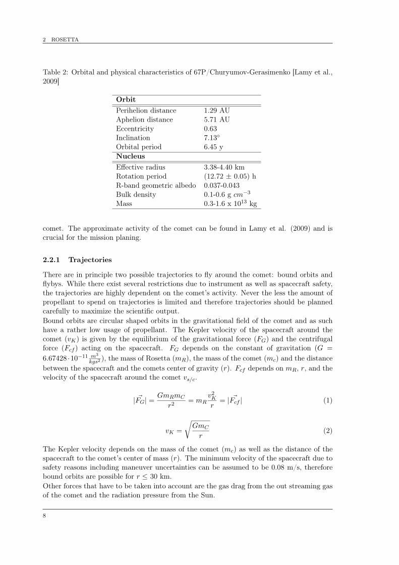
19 DFMS FM CEM scan of 13 u/e. Theses spectra are recorded with an emis-sion of 20 µA and an integration time of 1000 ms per step while CO2 wasintroduced into the chamber. In HR 13C and 12CH are clearly separated. . . 28
20 DFMS FM Faraday cup scan of 28 u/e for HR (left) and LR. The step widthfor both scans was 0.014 u/step. The emission was 200 µA and the integrationtime 1000 ms per step. . . . . . . . . . . . . . . . . . . . . . . . . . . . . . . 29
21 Remote Detector Package (RDP): on the left side from top to bottom RDP-CON, RDP-FEM, RDP-DVI and RDP-FLI. On the right side the defect anlater replaced inverter on the bottom side of the RDP-DVI board. . . . . . . . 30
22 The three effects observed for rowB of LEDA for FM. The drop down incounts can be the first ⇠20 pixels, a plateau where a peak is seen for rowAand the ’memory’ effect. The ’memory’ effect, shows still some signal on thesame pixels as the spectrum before the peak was located. . . . . . . . . . . . . 31
23 Ionization cross section of He, Ne and CO2 dependent on the electron energy.A maximum for the ionization cross section can be found for electron energiesof 70 – 100 eV. Data from Rice University (2013). . . . . . . . . . . . . . . . . 34
24 Fragmentation pattern comparison of CO2 for different electron energies inthe ion source, recorded with the MCP/LEDA. For discussion see text. . . . 35
25 The offset subtraction in principle for rowA. . . . . . . . . . . . . . . . . . . . 3826 Picture of an MCP with the hexagonal structure due to fabrication fashion.
The structure causes a modulation in the individual pixel gain of 24 pixelsfor the FM. . . . . . . . . . . . . . . . . . . . . . . . . . . . . . . . . . . . . . 39
27 FM individual pixel gain of rowA and rowB of the same species on the sameMCPFront (GS=14). To distinguish the two rows, rowB is plotted with anoffset of 0.1. No reliable corrections are given for the edges of the MCP, dueto data processing. . . . . . . . . . . . . . . . . . . . . . . . . . . . . . . . . . 40
28 FM individual pixel gain of row A on gain step 7 to 14. . . . . . . . . . . . . 4129 FM comparison of pixel gain recorded in 2009 and 2012, with a depletion in
the middle of the MCP of ⇠40%. . . . . . . . . . . . . . . . . . . . . . . . . . 4130 MCP gain for DFMS FM. The ’old’ gain are the gain values from the first
calibration [Langer, 2003a] and ’new’ gain are the values of the calibration inthis work. . . . . . . . . . . . . . . . . . . . . . . . . . . . . . . . . . . . . . . 45
31 CASYMIR: This figure shows a schematic view of the calibration facility. Theinstrument is docked on the right hand side after the bellows. The facilityallows introduction of the gas in two different ways: static mode and dynamicmode. In the dynamic mode, gas from the gas mixing unit in the upper leftand is introduced through the nozzle into V3. The beam is then skimmedbetween V3 and V2. An iris between V2 and V1 can reduce the area of thebeam. In V1 and V0 the beam can expand and is measured at the end ofthe docking section by an instrument. In the static mode gas is introducedinto V1 through a needle valve (LV4), while the V2 is separated from V1 bya closing a gate valve. . . . . . . . . . . . . . . . . . . . . . . . . . . . . . . . 50
32 The linearity between measured signal and the pressure for Ne. . . . . . . . . 53
vii/ix

LIST OF FIGURES
33 Comparison of DFMS isotopic measurements of 22Ne/20Ne with literaturevalues for the MCP/LEDA and CEM for all emissions. The agreement be-tween literature value and the measurements is with the exception of the LRmeasurement for the 2 µA with MCP/LEDA reasonable. . . . . . . . . . . . . 54
34 The linearity between measured signal and the pressure for Ar. . . . . . . . . 5635 Comparison of DFMS isotopic measurements of 36Ar/40Ar and 38Ar/40Ar
with literature values for the MCP/LEDA for all emissions. The agreementbetween literature value and the measurements is reasonable. . . . . . . . . . 57
36 Comparison of DFMS isotopic measurements of 36Ar/40Ar and 38Ar/40Arwith literature values for the CEM for all emissions. The agreement betweenthe literature values and the measurements are reasonable with the exceptionof the 2 µA 36Ar/40Ar measurements. . . . . . . . . . . . . . . . . . . . . . . 58
37 Comparison of DFMS isotopic measurements of 78Kr/84Kr, 80Kr/84Kr,82Kr/84Kr, 83Kr/84Kr and 86Kr/84Kr with literature values for the MCP/LEDAfor 200 µA emissions. The agreement between literature value and the mea-surements is reasonable. . . . . . . . . . . . . . . . . . . . . . . . . . . . . . . 59
38 Comparison of DFMS isotopic measurements of 78Kr/84Kr, 80Kr/84Kr,82Kr/84Kr, 83Kr/84Kr and 86Kr/84Kr with literature values for the CEMfor 200 µA emissions. The agreement between literature value and the mea-surements is reasonable. . . . . . . . . . . . . . . . . . . . . . . . . . . . . . . 60
39 Comparison of DFMS isotopic measurements of 124Xe, 126Xe, 128Xe, 129Xe,130Xe, 131Xe, 132Xe, 134Xe and 136Xe (relative to the most abundant isotope132Xe) with literature values for the MCP/LEDA for 200 µA emissions. Theagreement between literature value and the measurements is reasonable forthe lighter ions, however it does not agree for the two heaviest ions 134Xe and136Xe. A possible explanation can be found in the text. . . . . . . . . . . . . 61
40 Comparison of DFMS isotopic measurements of 124Xe, 126Xe, 128Xe, 129Xe,130Xe, 131Xe, 132Xe, 134Xe and 136Xe (relative to the most abundant isotope132Xe) with literature values for the FC for 200 µA emissions in low resolution.The agreement between literature value and the measurements is reasonablewith the exception of the less abundant isotopes 124Xe, 126Xe and 130Xe. Apossible explanation can be found in the text. . . . . . . . . . . . . . . . . . . 62
41 The fragmentation pattern for H2O measured with DFMS FM for MCP/LEDAand CEM. For comparison NIST4, Rao 1995 and Orient 1987 is given. Al-though for the latter two the electron energy of 45 eV was taken into account,they are not in agreement with the measurements of DFMS FM. Uncertaintiesof the measurements are due to average for all emissions. . . . . . . . . . . . 65
42 MCP/LEDA HR spectrum of mass 19 u/e, whereas H18O is clearly separatedfrom H17
2 O and HD16O. The Full Width at Half Maximum (FWHM) of thepeak to the right is significantly broader than that for H18O and impliestwo overlapping peaks. To resolve the latter, two Gaussian fits were applied;taking the FWHM from H18O as fixed for all three mass peaks and theamplitudes of H17
2 O and HD16O as the free parameters to be fitted. . . . . . 6743 Comparison of the DFMS measurements for 15N/14N with literature value
for the MCP/LEDA. 15N/14N ratio is measured for 15N14N relative 14N2. . . 6944 Fragmentation pattern for CO2 for the MCP/LEDA and the CEM compared
to NIST. . . . . . . . . . . . . . . . . . . . . . . . . . . . . . . . . . . . . . . . 70
viii/ix

LIST OF FIGURES
45 The measured isotopic ratios of CO2 with the MCP/LEDA for an emissionof 200 µA relative to literature value. . . . . . . . . . . . . . . . . . . . . . . . 71
46 The fragmentation pattern for CH4 for MCP/LEDA and CEM compared toNIST. Errorbars for MCP/LEDA and CEM are due to the average for allemissions. . . . . . . . . . . . . . . . . . . . . . . . . . . . . . . . . . . . . . . 73
47 Isotopic abundances measured with DFMS relative to literature values for CH4. 7448 The fragmentation pattern of C2H6 measured with the MCP/LEDA and the
CEM. For comparison NIST values are given. Error bars are due to standarddeviation of the average for all emissions. . . . . . . . . . . . . . . . . . . . . 76
49 Isotopic measurements of C2H6 with the MCP/LEDA (black) and the CEM(red). The measurements are in good agreement with literature value, how-ever the statistical uncertainties for the 13C/ 12C measured with the CEMare rather high. Mass 12 can only be measured with the CEM, therefore nomeasurements for the MCP/LEDA are available for 13C/ 12C . . . . . . . . . 77
50 Fragmentation pattern for C3H8 measured with MCP/LEDA and CEM, withthe average for all emissions compared to NIST. Error bars are due to standarddeviation of the average. . . . . . . . . . . . . . . . . . . . . . . . . . . . . . . 79
51 Isotopic abundances for C3H8 relative to literature value. . . . . . . . . . . . 8052 The fragmentation pattern for C4H10 measured with MCP/LEDA and CEM.
For comparison the values of NIST are given. Error bar are due to the stan-dard deviation of the average for all emission. . . . . . . . . . . . . . . . . . . 83
53 Isotopic abundances of C4H10 relative to literature. The measurements areperformed with an emission of 200 µA for the MCP/LEDA (black) and theCEM (red). The measurements are in good agreement with literature value. . 84
54 The fragmentation pattern for C2H4 measured with MCP/LEDA and CEM.For comparison the values found in NIST are given. Error bar are due to thestandard deviation of the average for all emission. . . . . . . . . . . . . . . . . 86
55 The isotopic abundances for C2H4 and C measured with the MCP/LEDA(black) and the CEM (red). All measurements are in good agreement withliterature. Error bars are discussed in the text. For C no measurements areavailable for the MCP/LEDA, because of the limited mass range. . . . . . . . 87
56 MCP/LEDA measurement in HR with an emission of 200 µA for the GCUgas. The GCU contains Ne, CO2 and Xe. The peaks around 66 u/e are thesignal of the doubly charged Xe. The signal of O and CO are the fragmentsof CO2. . . . . . . . . . . . . . . . . . . . . . . . . . . . . . . . . . . . . . . . 90
57 Measurement of a gas mixture containing Ne, Ar, Kr, and Xe measuredwith the MCP/LEDA in HR at an emission of 200 µA. The peaks marked asXe are due to the doubly charged Xenon. . . . . . . . . . . . . . . . . . . . . 93
58 MCP/LEDA measurement in HR with an emission of 200 µA for the CO2 +C3H8 mixture. HR spectra with a better resolution of the three highlightedpeaks can be found in Fig. 59. For a better overview the other fragments ofC3H8 are not highlighted but can be found in Tab. 32. . . . . . . . . . . . . . 96
59 The three spectra of the fragments and the parent molecule of both gases.MCP/LEDA measurement in HR with an emission of 200 µA for the CO2 +C3H8 mixture. . . . . . . . . . . . . . . . . . . . . . . . . . . . . . . . . . . . 97
ix/ix


1 INTRODUCTION
1 Introduction
The origin of planetary systems starts with the collapse of a molecular cloud (mainly hy-drogen), that compresses the matter in the center. A disc is formed around the center ofgravity because of the conservation of the angular momentum. In the center of the disc andfed from the gaseous and solid material falling inward from the disc a protostar starts toform. The protostar is heated because during the collapse gravitational energy is conversedinto kinetic energy. Once the temperature in the protostar reaches about 106 K, nuclearreactions are initiated and the protostar starts to burn [de Pater and Lissauer, 2001]. Inthe cooling process protoplanetary discs around it, elements and molecules undergo chem-ical reactions as a consequence of different temperatures and pressures. This non-trivialprocesses are difficult to understand because of uncertainties in the condensation sequenceand since non-equilibirum chemistry plays an important role especially in the cold outerregions of the protoplanetary disc [de Pater and Lissauer, 2001]. The remaining materialin the disc is then the start for planetesimals that might accrete material and grow toplanetary embryos. The most massive planetesimals have the largest gravitational crosssection and gain additional mass if the escape velocity does not exceed the relative veloc-ity of the surrounding objects. How bodies from centimeter- to kilometer-size were grownis still poorly understood [Irvine and Lunine, 2004]. Eventually planetary embryos gathermost of the solids through their gravitational influence and become planets. It is assumedthat gravitational and magnetic torques launch waves in the gas and dust. By compressingand heating material it might be that giant gaseous planets such as Jupiter and Saturn canform [Irvine and Lunine, 2004]. The only planetary system where detailed information isavailable is the solar system. The formation of the solar system occurred in a similar wayapproximately 4.6 Gyr ago.
Figure 1: The formation of the solar system as schematics: (a) The molecular cloud, (b)Collapsing of the molecular cloud and formation of a disc, (c) The protostar starts to form,(d) The protostar starts burning and planetesimals build in the disc, (e) The most massiveplanetesimals become planetary embryos, and (f) The planets are formed. Image credit:Penn State University (2013)
The planetary system contains the star close to the center and planets orbiting the barycenterof the system. The remaining planetesimals can be trapped by the planets and form moonsif not already formed during the accretion or stay loose in the form of e.g. the asteroid belt.
1

1 INTRODUCTION
A schematic overview of the solar system can be found in Fig. 2. The variety of objects in aplanetary system is not limited to stars, planets, and moons but contains a variety of smallerobjects: Dwarf planets, asteroids, and comets. The dwarf planets are the most massive smallobjects and are in hydrostatic equilibrium after accumulating enough material during planetformation process. The most popular dwarf planet is Pluto. These objects have typicallya diameter of a few hundred kilometers and can be seen as representatives of planetaryembryos. Ceres, also a dwarf planet because of its size, can also be seen as the largestasteroid in the asteroid belt [Jewitt et al., 2008]. The smaller bodies in the solar system areeither asteroids or comets, depending on their appearance at the sky. Asteroids are depletedin volatiles and consist mainly of refractory material. Therefore, asteroids don’t show signsof a sublimation driven atmosphere. Asteroids in the solar system can be found from insideMercury’s orbit to outside the orbit of Neptune [de Pater and Lissauer, 2001]. Most knownasteroids are concentrated between the orbits of Mars and Jupiter, known as the asteroidbelt. The depletion in volatiles in asteroids has long been regarded as a consequence of thesnowline concept. The snowline is commonly referred to as the heliocentric distance wherewater condenses and ice can be formed and is located between the orbit of Jupiter and Mars.Volatiles condensed at large heliocentric distances from the Sun during the condensationsequence of the protoplanetary disc. Closer to the Sun temperatures are higher and gaswas swept away during periods of high solar activity. Therefore asteroids show a depletionof volatiles. In the asteroid belt occasionally collisions between asteroids can happen andscatter objects towards the Earth as meteorites.
Figure 2: The schematic drawing of the solar system. From the lower left to the upper rightcorner: The planets of the solar system, the inner solar system with the orbits of the fourinner planets and the asteroid belt, the solar system with the Kuiper belt, and the Oortcloud. Image credit: Svitil and Foley (2004).
The comets are an other group of small bodies and consist of an ice rich nucleus with lowalbedo. The nucleus can produce a gravitationally unbound atmosphere (coma) that is
2

1 INTRODUCTION
mainly driven by sublimation from the surface of the nucleus. The apparent active area ofthe nucleus can be enlarged by icy grains that are lifted from the surface of the nucleus andsublimate [A’Hearn et al., 2011]. When the comet gets closer to the Sun, it starts to buildup a tail, containing ions and/or dust particles (see Fig. 3). Because of conservation ofangular momentum of the dust particles, they slow down as they are pushed away from thecomet by gas drag and solar radiation, resulting in a curvature of the tail in the oppositedirection of the comets motion [de Pater and Lissauer, 2001]. In contrast to this curvedshaped tail, the usually blueish tail consists of ions, neutrals, and points away from theSun. The ions are bound to the interplanetary magnetic field lines and dragged along withthe solar wind [de Pater and Lissauer, 2001]. Cometary orbits are eccentric ellipses, so thatonly a small fraction of the time on an orbit is spent in the inner planetary region. Cometsspend most of their time in the cold outer part of the solar system and are therefore believedto contain and preserve material from the formation of the solar system. There exist twomain population of comets according to their current location: The Oort cloud comets andthe Kuiper belt comets. The Oort cloud is a spherical distribution of comets at distancesof > 104 AU [de Pater and Lissauer, 2001]. The Oort cloud was postulated by Jan Oortdue to observations of dynamically ’new’ long-period comets. Because of the distributionof the semi-major axis and the inclination of the comets, that were observed at that timeand scattered into the inner solar system, Oort postulated a spherical shaped cloud as thereservoir and origin of this comets [de Pater and Lissauer, 2001].
The other reservoir is the Kuiper belt, a disc shaped distribution of icy bodies beyondthe orbit of Neptune, and these objects are therefore often referred to as Trans-NeptunianObjects. The Kuiper belt contains objects with low inclination orbits and is, based on dy-namical arguments, divided into several subgroups: The classical Kuiper belt objects havelow eccentricity orbits at heliocentric distances that are approximately 32 < a < 50 AU[Morbidelli and Brown, 2004] and stable over the age of the solar system. Gravitationalscattering of these objects by Neptune can cause highly eccentric orbits. An-other subset ofthe population of the Kuiper belt is in an orbital resonance of 3:2 with Neptune, the bestknown object thereof is Pluto. Comets originating from the Kuiper belt can be trapped byJupiter once they are scattered into the inner solar system and become short period cometsbeing called Jupiter family comets (JFC) [Jewitt et al., 2008].
The connection between the Oort cloud and the Kuiper belt was given by the discovery ofSedna (90377) with a high semi-major axis of 480±40 AU and a perihelion of 76±4 AU[Brown et al., 2004]. Since Sedna can be assigned neither to the Kuiper belt nor to thedistant Oort cloud it must therefore be a transitional object of the inner Oort cloud.
For completeness a third group of possible comets is mentioned, the main belt comets (MBC).These comets have orbits in the main asteroid belt between Mars and Jupiter. Theseobjects can show dust tails or even persistent dust emissions over timescales of months[Jewitt et al., 2008]. These outbursts were long believed to originate from collisions butmight represent another population of comets although they might also be captured cometsfrom other regions.
Small bodies have experienced relatively little changes since their formation, compared toplanets or dwarf planets, that underwent alteration due to collisions and differentiation.Comets build behind the snowline and the amount of volatiles incorporated is therefore
3

1 INTRODUCTION
supposed to be high, and since they spend most of their life time far away from the Sunat low temperatures, comets are thought to contain the most pristine material in the so-lar system. Due to low temperatures at large heliocentric distances, there might havebeen even an incorporation of pristine dust particles in comets which are older than thedark molecular cloud [de Pater and Lissauer, 2001]. The Nice model [Gomes et al., 2005,Tsiganis et al., 2005, Morbidelli et al., 2005], postulates that the gas giants underwent or-bital migration and forced objects in the asteroid belt and/or Kuiper belt on eccentric orbitsthat put them in the path of the terrestrial planets. During this late heavy bombardmentcomets might have brought water and even pre-biotic molecules to Earth and Mars. How-ever, the role of comets as a source of water on Earth was long questioned, or at least thoughtto be of limited importance because of the different D/H ratios found in comets compared toEarth (e.g. Halley: Balsiger et al. (1995) and Eberhardt et al. (1995)). But recent remotesensing measurements of comet 103P/Hartley 2 (see Fig. 4) by the Herschel Space Obser-vatory found an ocean-like D/H ratio [Hartogh et al., 2011] and might bring back cometsas possible sources for water on Earth. However, the measurements of one Jupiter familycomet is a fairly small sample. Further in situ measurements with instruments that providethe D/H ratio in water at a comet that originates in the Kuiper belt might shed more lighton the riddle about the origin of the water on terrestrial planets.
Figure 3: Comet Hale-Bop with the straightion tail in blueish and the slightly curved dusttail. Image credit: Jewitt et al. (2008)
Figure 4: The greyish nucleus of comet Hart-ley 2 and belongs to the group of JFC. Imagecredit: NASA/JPL-Caltech/UMD
4

2 ROSETTA
2 Rosetta
Rosetta is a planetary cornerstone mission of the European Space Agency (ESA). The nameof Rosetta originates from the famous Rosetta Stone. The reason for the naming is givenin Berner et al. (2002) and a summary thereof shall be given here: the stone was found byFrench soldiers in 1799 near the village Rashid (Rosetta) in Egypt’s Nile delta when theyprepared to destroy a wall. The stone is made of granodiorite, a rock similar to granite, withan inscription. The inscriptions on the stone were identified as three different languages:hieroglyphs, Egyptian demotic, and Greek. While the hieroglyphs were more of a languagein pictures for the priests, the demotic represents the written language of ancient Egyptpeople. By comparing the inscription it became clear that the three parts in three differentlanguages contained essentially the same text with minor differences. Therefore the stoneprovided the key to the modern understanding of the Egyptian hieroglyphs and the historyof a long lost culture.Similar to the discovery of the Rosetta stone eventually leading to the deciphering of thehieroglyphs, the Rosetta mission will help scientist to unravel some of the mysteries ofcomets, in particular 67P/Churyumov-Gerasimenko. Comets are considered to be the mostprimitive objects in the solar system and the building blocks from which planets are formed,similar to the hieroglyphs as building blocks of the Egyptian language. Comets still containices and dust present in the original solar nebula at the time of their formation and thereforegrant a unique glimpse into the conditions when our solar system emerged.
2.1 The Mission
The first and very successful ESA comet mission was Giotto which flew by comet 1P/Halleyin 1986 and the Rosetta mission is the logical continuation of ESA’s comet investigations.In the mean time there were several NASA missions to comets, e.g. Wild 2 with Stardust inencounter 2004 and Hartley 2 with Deep impact encounter 2010. The main scientific objec-tive of Rosetta is to investigate the origin of the solar System through the close inspectionof a comet by means of orbiter and probe. A detailed description of the Rosetta mission canbe found in Schulz et al. (2009). The Rosetta spacecraft consists of an orbiter and a landercalled Philae. The Rosetta spacecraft was launched in March 2004 by an Ariane-5G+ fromKourou (French Guiana) more than one year after scheduled departure. This was due toan Ariane failure in December 2002, causing the postponement of the launch. The targetwas switched from comet 46P/Wirtanen to 67P/Churyumov-Gerasimenko. To gain enoughenergy to match the orbit of the comet, several gravity assists were performed at Earthand Mars. Rosetta will escort 67P/Churyumov-Gerasimenko from more than 3 AU in he-liocentric distance, when the cometary activity is still very low to past perihelion (maximalactivity). During the encounter the lander will be first released for a close investigation ofthe nucleus while the orbiter will orbit around the comet and investigate the comet with un-precedented precision. The notable milestones of the mission during the 10 years of voyageand the following investigation of the comet are summarized in Tab. 1.The gravity assists at the planets were required to gain enough energy to reach the orbit of67P/Churyumov-Gerasimenko and were a chance to test the scientific instrument package.In addition they represent a great possibility to keep up the general public interest over thelong mission duration. The scientific highlights during the mission are, besides the closeinvestigation of the comet, two asteroid flybys: 2687 Steins and 21 Lutetia (see Fig. 5).Documentation of the two successful asteroid flybys of Steins and Lutetia can be found in
5

2 ROSETTA
Table 1: Milestones of the Rosetta mission.
Mission events DateLaunch in Kourou 02.03.20041. Earth gravity assist 04.03.2005Mars gravity assist 25.02.20072. Earth gravity assist 13.11.20072867 Steins flyby 05.09.20083. Earth gravity assist 13.11.200921 Lutetia flyby 10.07.2010Rendezvous maneuver 1 23.01.2011Start hibernation 08.06.2011Wake up from hibernation 20.01.2014Rendezvous maneuver 2 22.05.2014Orbit around 67P Sept. 2014Lander (Philae) delivery 11.11.2014Perihelion Passage Aug. 2015Nominal end of mission 31.12.2015
Keller et al. (2010) for Steins and in the special issue of Schulz et al. (2012) for Lutetia andare not further discussed in this work.Rosetta is the first spacecraft to cross the Jovian orbit using solar cells as its main powersource. However during deep space cruise, the spacecraft is placed in hibernation with mostelectrical systems switched off to limit consumption of power and fuel. After the wake-upfrom hibernation in January 2014 the spacecraft will perform a rendezvous maneuver toreach the orbit of the comet. A series of measurements before and after lander delivery willbe performed to safely release the lander on the comet’s surface. Once the lander reaches thesurface, it will be the first controlled touch down of a man-made probe on the nucleus of acomet and its close and detailed investigation with combined forces of orbiter and lander canbegin. The measurement goals of the Rosetta mission include [Schwehm and Schulz, 1999]:
• Global characterization of the nucleus, it’s surface morphology and composition
• Determination of the dynamical properties of the nucleus
• Determination of chemical, mineralogical, and isotopic composition of volatiles andrefractories in the cometary nucleus
• Determination of the physical properties and interrelation of volatiles and refractoriesin the cometary nucleus
• Studies of the development of cometary activity and the processes in the surface layerof the nucleus and inner coma, that is dust/gas interaction
• Studies of the evolution of the interaction region of the solar wind and the outgassingcomet during perihelion approach.
These prime objectives are, if successfully accomplished, considered to be crucial to addresskey questions of the origin and formation of the solar system.
6

2 ROSETTA
Figure 5: Left : Asteroid Lutetia at closest approach. Right : Lutetia in conjunction withSaturn. Image credits: ESA 2010 MPS for OSIRIS Team MPS/UPD/LAM/IAA/RSSD/IN-TA/UPM/DASP/IDA
2.2 67P/Churyumov-Gerasimenko
Comet 67P/Churyumov-Gerasimenko was first discovered in 1969 by Klim Ivanovic Churyu-mov and Svetlana Ivanova Gerasimenko. The comet could be observed to this day on sevenperihelion passages (last perihelion passage 28. February 2009 [Lara et al., 2010]). Thecomet is classified as a short period comet of the Jupiter Family Comet class, based on itsorbital period of 6.45 y and the aphelion distance of 5.7 AU [JPL, 2013]. The origin ofJFC’s is believed to be the Kuiper Belt, where gravitational encounters with outer planetslet them migrate into the inner solar system. The orbits of JFC’s are controlled by Jupiter,while orbital elements can be significantly changed by repeated encounters with Jupiter.It is known through backwards calculations [Lamy et al., 2009], that the orbital elementsof 67P/Churyumov-Gerasimenko have significantly changed after a close encounter withJupiter (at a distance of only 0.0518 AU) in 1959, resulting in a perihelion change from2.78 AU to 1.28 AU, increasing eccentricity from 0.36 to 0.63, and shortening of the orbitalperiod from 8.97 to 6.55 y. An overview of the current orbital elements can be found in Tab.2.The comet 67P/Churyumov-Gerasimenko (67P) had emerged as favorable alternative to theinitial target 46P/Wirtanen, after cancellation of the original Rosetta launch in January2003. In the following the target of Rosetta became the subject of several ground-basedas well as space-borne (e.g. Hubble Space Telescope) observations. The result of theseobservations lead to sufficient knowledge about the physical characteristics of the maintarget to plan the mission. However these properties will be updated once Rosetta is at the
7
2 ROSETTA
Table 2: Orbital and physical characteristics of 67P/Churyumov-Gerasimenko [Lamy et al.,2009]
OrbitPerihelion distance 1.29 AUAphelion distance 5.71 AUEccentricity 0.63Inclination 7.13�
Orbital period 6.45 yNucleusEffective radius 3.38-4.40 kmRotation period (12.72 ± 0.05) hR-band geometric albedo 0.037-0.043Bulk density 0.1-0.6 g cm�3
Mass 0.3-1.6 x 10¹³ kg
comet. The approximate activity of the comet can be found in Lamy et al. (2009) and iscrucial for the mission planing.
2.2.1 Trajectories
There are in principle two possible trajectories to fly around the comet: bound orbits andflybys. While there exist several restrictions due to instrument as well as spacecraft safety,the trajectories are highly dependent on the comet’s activity. Never the less the amount ofpropellant to spend on trajectories is limited and therefore trajectories should be plannedcarefully to maximize the scientific output.Bound orbits are circular shaped orbits in the gravitational field of the comet and as suchhave a rather low usage of propellant. The Kepler velocity of the spacecraft around thecomet (vK) is given by the equilibrium of the gravitational force (FG) and the centrifugalforce (Fcf ) acting on the spacecraft. FG depends on the constant of gravitation (G =
6.67428 ·10�11 m3
kgs2 ), the mass of Rosetta (mR), the mass of the comet (mc) and the distancebetween the spacecraft and the comets center of gravity (r). Fcf depends on mR, r, and thevelocity of the spacecraft around the comet vs/c.
~|FG| =GmRmC
r2= mR
v2Kr
= ~|Fcf | (1)
vK =
rGmC
r(2)
The Kepler velocity depends on the mass of the comet (mc) as well as the distance of thespacecraft to the comet’s center of mass (r). The minimum velocity of the spacecraft due tosafety reasons including maneuver uncertainties can be assumed to be 0.08 m/s, thereforebound orbits are possible for r 30 km.Other forces that have to be taken into account are the gas drag from the out streaming gasof the comet and the radiation pressure from the Sun.
8

2 ROSETTA
The gas draga depends strongly on the gas flux coming from the comet as well as the exposedarea of the spacecraft and is pointing away from the comet.The gas flux coming from the comet is the gas density multiplied by the gas velocity (vgasb). The gas density depends on the activity of the comet, Q,vgas, and r. The affected area ofthe spacecraft is the area of the cube plus the exposed area of the solar panels and, since thesolar panels are always perpendicular to the Sun, this area is known. The area depends onthe sub-solar angle of the spacecraft. The gas drag is always pointing away from the comet,however, this is the most difficult force to predict since the out-streaming gas is not likelyto be spherically symmetric and the absolute activity is difficult to predict. The radiationpressure exerted by the Sun depends on the affected area of the spacecraft as well as thedistance from the Sun. The affected area is always the full cross-section of the solar panelsand the spacecraft body while the distance between the comet and the Sun (and thereforebetween spacecraft and Sun) decreases. This force will therefore increase during the journeyof the comet towards the Sun and is always pointing away from the Sun.Restrictions due to spacecraft safety are: position and maneuver uncertainties, the avoidanceof the shadow of the comet (no power), the platform where the radiators and the landeris/was mounted should not be exposed to the Sun at a distance < 2.2 AU, the safety duringa failure mode while the spacecraft is proceeding on the flight path till it can be recovered.The navigation camera needs a reference point within its field of view and should avoid thedirect sunlight.
Figure 6: Kepler velocity depending on cometocentric distanceand the mass of the comet.
Furthermore the follow-ing important parametersneed to be consideredfor planning: spin axisof the comet, seasons ofthe comet, the cumula-tive flux of the trajec-tories (given by 1/r2 xtime spent) and last butnot least time and point-ing uncertainties of thespacecraft as well as themeasurements.Bound orbits are possiblein the terminator plane(plane between night andday side of the comet)with a maximal tilt angleof < 30� (due to the nav-igation camera) at a dis-tance (r) 30 km witha velocity relative to the
afor one dimensional case: |gas drag| = 12 cdmg
n
g
�
s/c
(vgas
�v
s/c
)2 with c
d
: drag coefficient, mg
: mass ofthe gas [kg], n
g
: density of the gas [particle/cm3], �s/c
: exposed area of the spacecraft [m2], vgas
: velocityof the gas [m/s], and v
s/c
: velocity of the spacecraft [m/s].bThe velocity of the spacecraft relative to the velocity of the out streaming gas but since the velocity of
the out streaming gas is in the order of several 100 m/s while the velocity of the spacecraft is in the orderof a few m/s the latter can therefore be neglected.
9

2 ROSETTA
comet of vK . A possible trajectory of bound orbits is given in Fig. 7. The radiation pressurein the terminator plane is the same for every position on the orbit, the gravitational force,centrifugal force, and the gas drag should be in equilibrium. Therefore the time spent inbound orbits is highly dependent on the comet’s activity and will be performed in the earlyphase of the mission when the gas drag is low.
Figure 7: Bound orbit around the comet in the terminator plane. +X points from thecomet’s center towards the Sun, Y is in the ecliptic plane.
The flyby trajectories can further be divided into two groups: close flybys and far flybys.The flyby velocity has to be two times higher than vK because of spacecraft safety. Thereason for this is, that the spacecraft is always above the escape speed if it goes into safemode. For close flybys the distance to the comet’s center is r > 8km. The navigation cameramust be able to see the full comet. The distance is higher for far flybys. A flyby over thesub solar point (Sun is shining on the bottom of the spacecraft, temperature sensitive!) canonly be performed at Sun distances of > 2.2 AU therefore some type of flybys have to beperformed before reaching this distance to gain knowledge about the most exposed area tothe Sun and to get the full phase curve. However, flybys will be mainly performed while thecomet is more active and bound orbits are no longer possible.The knowledge of the exact position of the spacecraft as well as the Solar Aspect Angle(SAA) is of fundamental importance to interpret the scientific data. Spacecraft attitudeand position can be accessed through NASA’s SPICE toolkit.SPICE c (Spacecraft, Planetary, Instruments, C-Matrix, Events) is a powerful tool offeredby NASA’s Navigation and Ancillary Information Facility (NAIF) for NASA flight projectsand NASA funded researchers to assist scientists in planning and interpreting observationsfrom space-based instruments aboard robotic spacecrafts. The Rosetta mission to comet67P/Churyumov-Gerasimenko is also supported through this tool. The SPICE tool is avail-able in different programmer languages and transforms vectors from one coordinate systeminto another as well as a lot of other applications, e.g. closest approach of two objects and
cfor detailed documentation see: http://naif.jpl.nasa.gov/naif/index.html
10

2 ROSETTA
Figure 8: SAA for Rosetta during the Lutetia flyby. CA marks the closest approach ofRosetta at 15:45 UTC (2010-07-10). The angle between the +Y-axis and the Sun (Y ) isnominal 90� since the solar panels are always exposed to the Sun. The angle between the+Z-axis and the Sun (Z) and X are always 180� in total.
many more. The tool comes with a set of different problems to be solved by test programs.The user is guided within documentations as well as examples. The SPICE tool can be di-vided into two subsections, one: the necessary kernels containing all the transformations andpositions, and two: the code to extract the necessary data. The kernels contain knowledgeabout the coordinate system definition, data of trajectories, and time corrections. The SAAis especially important for the background problem of the gas cloud around the spacecraft[Schläppi et al., 2010] and therefore the interpretation of the data. The position of Rosettarelative to the comet is essential for the global mapping of the coma. Given as an examplein Fig. 8 is the SAA during the Lutetia flyby. Documentation of the code as well as thenecessary kernels are given in the App. A (SAA) and B (Trajectories).
2.2.2 Cumulative flux for different trajectories
Instruments measuring dust particles or gaseous species around the comet are especiallyinterested in the cumulative flux along a given trajectory. To gather as much signal aspossible, these instrument teams are interested in the total number of particles that enterstheir instrument. To deduce the flux for particles at a given location around the cometat a specific heliocentric distance there exist different approaches. The Haser model as-sumes spherical outgassing from the comet into the coma [Haser, 1957]. The distributionof the secondary species, produced by photodissociation of parent molecules and destroyedby photo-destruction processes, can be described by the Haser model [Combi et al., 2004].
11

2 ROSETTA
Assuming spherical outgassing, the density around the comet depends on the productionrate of the species (Q), the distance of the spacecraft to the comet (r), the gas velocity ofthe species (vgas), and the ionization scale length (�). The density of the parent species (n)can be calculated in the following way:
n(r) =Q · e
r
�
4⇡ · r2 · vgas(3)
With this model the distance to the comet where the density is dominated by parent speciesor daughter species can be deduced.
To compare the expected signal for different trajectories for in situ particle instruments, thecumulative flux has to be estimated. Neglecting the loss of parent species trough photoion-ization and dissociation (and vs/c « vgas) we can integrate Eq. 3 from closest approach to agiven point in time (te) to obtain the total cumulative flux of all parent species:
�flyby =
Z te
0
Q · vgas4⇡(vs/c · t+ r0)2 · vgas
dt =Q · arctan(vs/c·ter0
)
4⇡ · r0 · vs/c(4)
vs/c is the spacecraft velocity, vgas the gas velocity, r0 the minimum distance for the flyby,and te is approximately 3.5 days. For the full flyby the resulting cumulative flux has tobe doubled (due to the symmetry the same cumulative flux arises form -3.5 days to closestapproach). To scale the different integrated fluxes a time duration of 14 d per segment wastaken. Over the duration of one segment two far flybys can be performed and one closeflyby. The duration of a close flyby while collecting material is the same as for a far flybybut half of the segment time is used to fly back to a similar distance relative to the comet.The density of the comet at these distances is very small compared to that at the close flybydistance and therefore the additional flux collected over this time can be neglected.The cumulative integrated flux for the segment duration of a bound orbit with the assump-tion of spherical symmetry of the comet’s activity (Q) and the distance to the comet (r)is:
�Orbit = n · vgas · te =Q · vgas · te4⇡ · r2 · vgas
=Q · te4⇡ · r2 (5)
To calculate and compare the different fluxes collected during trajectories the total produc-tion rates for a low active comet were used (see Tab. 3).
Table 3: Total production rates for a low (LAC) and a high (HAC) active comet representingpossible scenarios for 67P/Churyumov-Gerasimenko at different heliocentric distances.
Heliocentric Distance [AU] LAC [1/s] HAC [1/s]1.24 (Perihelion) 4.14 x 1027 1.13 x 1028
2.00 4.60 x 1026 2.50 x 1027
3.00 3.70 x 1025 5.40 x 1026
3.50 2.10 x 1025 3.80 x 1026
Fig. 9 shows the different cumulative fluxes for representative trajectories. The bound or-bits are favored for the time where the comet starts to get active because the dust and gas
12

2 ROSETTA
instruments can collect more material than during flybys. When the comet gets more activeand bound orbits are no longer feasible because of the gas drag pushing the spacecraft awayfrom the comet, flybys are performed and far flybys are favored over close flybys with aclosest approach of 30 km, since two far flybys can be performed per segment as opposed toone close flyby and the dust and gas instruments can collect more material.
The cumulative fluxes increase much less (factor of six) than the activity of the comet (factorof 100 and more) because the flyby distances have to be increased for spacecraft safety andnavigation due to the higher gas drag. An other restriction is the propellant available, whilefor bound orbits a minimal amount of propellant (�v) is used, far flybys use more propellantdepending on the flyby velocity. Close flybys are even more �v consuming because of thehigher flyby velocity: for safety reasons the spacecraft has to fly always double the Keplervelocity to avoid a collision course with the comet, even if the spacecraft goes into a safemode. However, regardless of the trajectory the dust and gas instruments can only collectmaterial that enters the instrument, therefore the comet should be in the field of view.Therefore the comparison presented here is based on rough assumptions but gives a goodoverview.
Figure 9: Cumulative flux for different trajectories depending on the activity of the cometand therefore on the heliocentric distance for a low active comet (LAC see Tab. 3).
In case of non-sperically symmetric outgassing patterns, bodies, and forces have to be takeninto account, it is required to employ more complicated and higher dimensional models.Among these are fluid-type approaches [Crifo and Rodionov, 1997] or Direct SimulationMonte Carlo models [Tenishev et al., 2008, Tenishev, 2011]. Detailed results of the lattercan be accessed through the ICES tool which allows access to pre-computed simulationsobtained for comet 67P/Churyumov-Gerasimenko [University of Michigan, 2013].
13

2 ROSETTA
2.3 Payload
Table 4: Rosetta Payload. Detailed description for every instrument can be found in theRosetta book Schulz et al. (2009)
Name Instrument CategoryORBITERALICE UV spectroscopy Remote sensingCONSERT Radio sounding, nucleus tomography Nucleus large-scale structureCOSIMA Dust mass spectrometer (SIMS) Coma compositionGIADA Dust velocity and impact momentum Dust flux and mass distributionMIDAS Grain morphology with AFM Coma compositionMIRO Microwave spectroscopy Remote sensingOSIRIS Multi-color imaging Remote sensingROSINA Neutral and ion mass spectrometry Coma compositionRPC Plasma Consortium Comet plasma environment &
SW interactionRSI Radio Science Instrument Radio ScienceSREM Radio environment monitor Radio ScienceVIRTIS VIS and IR mapping spectroscopy Remote sensingLANDERAPXS ↵-particle-X-ray spectrometer Nucleus compositionCIVA Panoramic camera, IR microscope Nucleus surface structureCONSERT Comet nucleus sounding Nucleus structureCOSAC Evolved gas analyzer Nucleus compositionMUPUS Surface and Subsurface science Nucleus structurePTOLEMY Isotopic composition sampling Nucleus compositionROLIS Descent camera Nucleus surface structureROMAP Magnetometer, Plasma monitor Nucleus structureSD2 Sampling and distribution Nucleus structureSESAME Surface investigation Nucleus surface structure
In order to fulfill the mentioned mission objectives the Rosetta orbiter carries a set oftwelve scientific instruments to the coma of the comet as well as ten scientific instrumentsmounted on the lander Philae to the comet’s nucleus. The Rosetta orbiter is a cube shapedframe of 2.8 x 2.1 x 2.0 m3 (Fig. 10). Most of the scientific instruments are mounted onthe platform mainly pointing in the direction of the comet (+Z-direction). On both sidesof the central cube (in ±Y-direction), huge solar panels of 32 m2 each guarantee powersupply of 850 W even at large heliocentric distances of 3.4 AU [Glassmeier et al., 2009].The construction holding the solar panels as well as the central cube are mainly made fromhoneycomb structures. Most of the spacecraft as well as the instruments are covered in multi-layer insulation (MLI) foil, while the spacecraft is vented in the -Z-direction away from theinstruments. For communication with the Earth and data delivery a controllable high gainparabolic antenna of 2.2 m diameter is mounted on the opposite side of the lander (+X-direction). The lander is mounted on the -X side of the spacecraft and therefore shielded fromdirect sunlight most of the time. The spacecraft is three axis stabilized and the orientationis controlled by 24 thrusters with 10 N each. The altitude of the spacecraft is controlled
14

2 ROSETTA
by a set of navigation sensors as well as four reaction wheels. The Rosetta spacecraft has atotal launch mass of 2.9 t, while 1.72 t thereof is propellant. 165 kg is scientific payload andthe lander weight 100 kg [Glassmeier et al., 2009]. An overview of the scientific payload ofthe orbiter and the lander can be found in Tab. 4 [Glassmeier et al., 2009].
Figure 10: The orbiter of Rosetta, with the ROSINA instruments highlighted. The +Z-direction points away from the instrument platform and is supposed to point most of thetime towards the comet [Schläppi et al., 2010].
2.4 ROSINA
The Rosetta Orbiter Spectrometer for Ion and Neutral Analysis (ROSINA) is an instrumentpackage to determine the elemental, isotopic and molecular composition of the cometary at-mosphere and ionosphere and the physical properties (temperature, velocity) of the neutraland ionized components in the coma of comet 67P/Churyumov-Gerasimenko. The measure-ments of the isotopic composition in the volatile light elements (C, H, O, and N) in thecometary coma are difficult, because low abundance isotopes of these elements, (e.g. D,13C, 17O, 18O, 15N) are within a very close mass range of very abundant isobaric hybrides(H2, 12CH, 16OH, H16
2 O, 14NH) and a mass resolution m/�m of up to 3000 at 1% peakhight is needed to separate e.g. 13C from CH. The 13C/12C ratio is key for nearly everysolar system model. To accomplish these objectives, ROSINA (for detailed description seeBalsiger et al. (2007)), consisting of two mass spectrometers and a pressure sensor will fullfillthis task due to its unprecedented capabilities for space borne mass spectrometers:
• mass range of 1 u/e to > 300 u/e to detect simple atoms as well as heavy organicmolecules
• very high mass resolution of m/�m = ⇠3000 at 1 % peak height to resolve e.g. 12C16Ofrom 14N2 and 13C from 12CH
• wide dynamic range of up to 1010 and very high sensitivity of > 10�5 A/mbar
15

2 ROSETTA
The strategy to fly two mass spectrometers and a pressure sensor in a package has not onlytechnical advantages, but with regard to the long mission duration also provides redundancy.The three sensors are commanded and controlled by the Digital Processing Unit (DPU). TheROSINA sensor package is in total 1/5 of the mass of the total payload weight of the orbiter.Since the launch of Rosetta was postponed, the flight models of ROSINA could be replacedby the flight spare models. The advantage of this was, that the later built models could beflown. During building of the instruments one gains more knowledge about the process andthe later build instruments are usually in a better condition than the first version. Thereforethe model used in the lab is the original Flight Model (FM) while the original Flight Spare(FS) is on Rosetta.
2.4.1 COPS
The COmetary Pressure Sensor (COPS) is designed to measure the neutral gas parameters(density and velocity) around the comet. It consists of two gauges (see Fig. 11): thenude gauge and the ram gauge. The nude gauge is designed to measure the total neutralgas density, while the ram gauge measures the molecular flow. The combination of bothmeasurements provides knowledge about the total particle density and the gas velocity ofthe cometary volatiles. COPS is not only a scientific instrument but serves also as safetyfor the two mass spectrometers as well as other instruments, where an increase in pressure(e.g. > 10�6 mbar) can cause damage through high voltage discharges and thus have to beswitched off.
Figure 11: COmetary Pressure Sen-sor (COPS). Image credit: Balsigeret al. (2007)
The nude gauge is technically build in a Bayard-Alpert design, where neutrals are ionized trough elec-tron impact ionization. The ions are then acceler-ated towards a cathode for collection and the result-ing current is measured by a sensitive electrometer.The cathode is made of a thin molybdenum wire andthe measured current of the electrometer is directlyproportional to the total neutral particle density, theproportionality however is species dependent.The ram gauge measurement principle is similar tothe nude gage. The neutral gas is thermalized withinan equilibrium chamber in front of the ionization vol-ume. This measurement is very temperature sensitiveand therefore microtip field emitters are used insteadof the hot cathode of the nude gauge. The gaugesare mounted on booms in order to minimize interfer-ence with the spacecraft. The COPS sensor then ismounted on the instrument platform while the nudegauge exceeds the instrument platform and the ramgauge points in the direction of +Z. The nude gauge has a field of view of roughly 4⇡ (ex-cluding the direction of the boom). The ram gauge measures a ram pressure in +Z direction(dynamic pressure), and with the difference in dynamic and static (nude gauge) pressurethe gas velocity can be derived.
16

2 ROSETTA
2.4.2 RTOF
The Reflectron-Time-of-Flight mass spectrometer (RTOF) is one of the mass spectrometersof ROSINA (see Fig. 12). All TOF instruments are based on the same principle: Allparticles start at the same time (pulse), are accelerated to the same energy, fly along apotential free drift path, and are then detected time dependent at the detector. Because allthe particles undergo the same acceleration potential and therefore have the same energy,heavier ions (larger mass to charge (m/q) ratio) are slower than lighter ions resulting in alonger time of flight of a given distance. The instrument performance is manly dependent onthe fast electronics of the detector. To further enhance the resolution of the instrument, thetime between the particles has to be increased, this is achieved by a longer flight distance.The flight time is directly proportional to the flight distance (for a constant velocity) andtherefore a longer flight distance results in a higher resolution. This can be achieved with afold of the trajectory using reflectrons as done for RTOF. RTOF covers a mass range of 1u/e to >300 u/e and has a high sensitivity. RTOF can record a spectrum of the entire massrange almost simultaneously and within the nominal integration time of 200 s.
Figure 12: Reflectron-type Time of Flight mass spectrometer (RTOF)
2.4.3 DFMS
The Double Focusing Mass Spectrometer (DFMS) is the main subject of this work and adetailed description can be found in Chapter 3. RTOF and DFMS are designed to provideredundancy and both instruments together fulfill the primary objectives of ROSINA. WhileRTOF has a larger mass range (1 u/e – 300 u/e), DFMS complements it with the requiredmass resolution of m/�m = ⇠ 3000 at 1% peak height.
2.4.4 DPU
The Digital Processing Unit (DPU) is the control unit of the three ROSINA sensors (seeFig. 13). It commands the measurement modes for each instrument and handles the sciencedata. Furthermore it is the interface between the spacecraft and ROSINA.The principal drivers of the DPU design: optimum use of the allocated telemetry rate,single-failure tolerance for all functions serving more than one sensor, and the independenceof availability of radiation hardened parts. The primary data rate during full operationof all three sensors exceeds the maximum telemetry rate of the spacecraft by magnitudes.
17

2 ROSETTA
Reducing the amount of scientific data is therefore a fundamental need. A compressionof the data can be done in two levels, one in the sensor electronics itself and second inthe subsequent software processing by spectrum windowing or averaging, either in losslessor lossy fashion. The lossy compression can cause degradation in mass resolution and/ortime resolution but on the other hand is more powerful in deducing the file size (and thustelemetry) of the obtained science spectra.
Figure 13: Digital Processing Unit (DPU). Image credit: Balsiger et al. (2007)
18

3 DFMS INSTRUMENT DESCRIPTION
3 DFMS instrument description
DFMS is a double focusing mass spectrometer with an unprecedented high mass resolutionof m/�m ⇠3000 at 1% peak height for (in situ) space science [Balsiger et al., 2007]. It canmeasure ion and neutral densities of 1 cm�3 and has a dynamic range of ⇠1010. The sensorcan be divided into two parts: the instrument and the electronics box. The electronics boxis a compact part located under the instrument which is directly attached to the spacecraft.The whole sensor except the ion source is covered in Multi Layer Insulation (MLI). The MLI
Figure 14: DFMS FM
is designed to passively control the thermal behavior of DFMS. The nominal temperaturerange for DFMS to be operated is between -20 �C and +50 �C [Zahnd, 2002]. The MLI canhelp to heat the instrument into the operation range, since the temperature at the beginningof the mission is expected to be lower. The instrument itself has also heaters for examplein the RDP-electronics to heat the MCP/LEDA. The MLI shields the ions to be measuredby the instrument from the electric and magnetic fields of DFMS. The sensor is locatedon the instrument platform of Rosetta, with the field of view (FOV) of the instrumentaligned perpendicular to the instrument platform and pointing away from the spacecraft(+Z direction). The instrument platform of Rosetta is intended to point towards the comet.A sealed cover over the entrance of the instrument protects it during mounting on thespacecraft as well as avoiding contamination from Earth. The seal of the cover is brokenopen after launch and the cover mechanism can move the cover away from the entrance.The cover is mostly open during flight for safety reasons.A particle (ion or neutral) undergoes the following sections in DFMS: Ion source, transferoptics, analyzer sections, zoom optics and finally ends up in one of the three detectors.
19

3 DFMS INSTRUMENT DESCRIPTION
In the ion source neutrals are ionized by electron bombardment, while for external generatedions the source works as attractor for these ions. After this, ions (as well as the formerneutrals) are extracted to the analyzer section through the transfer optics. Depending onthe resolution mode of the spectrum the ions are focused on one of two slits in front of theanalyzer section. For high resolution (HR) the slit is narrower than for low resolution (LR).The analyzer section of DFMS is designed according to the Nier-Johnson geometry [Johnsonand Nier, 1953] in which a deflection of 90� in a radial electrostatic field analyzer (ESA)is followed by a magnetic deflection of 60�. Such a geometry leads to a compensation ofthe energy dispersion between electrostatic and magnetic fields, which results in an energyand direction focusing. After the analyzer section, only ions with the right mass to chargeratio (m/q) reach the zoom optics. In this section the focal point on the focal plane canbe adjusted by a hexapole or the image scale can be increased by a combination of twoquadrupoles. Finally the ions are detected by the main detector, a combination of a MicroChannel Plate and a Linear Detector Array (MCP/LEDA) or on one of the two additionaldetectors, the Channel Electron Multiplier (CEM) or the Faraday Cup (FC).
3.1 Ion source
Figure 15: Picture of DFMS ion source with the ion source axis and the main FOV of 20� x20�. For a better understanding of the position of the FOV the axis of the spacecraft frameare added.
The ion source has a main FOV of 20� x 20� and is centered in the ion source axis whichlies parallel to +Z, while the narrow angle FOV (2� x 2�) is perpendicular to the sourceaxis and parallel to the +X, see Fig. 15. The ion source can be operated in one of twomodes: the neutral mode or the ion mode. An overview of the ion source potentials andthe electrodes can be found in Fig. 16. In the neutral mode neutrals are ionized by electronimpact ionization. While externally formed ions are efficiently prevented from entering theion source by floating the ion source on a positive potential of +200 V on the ion source boxpotential (ISB) (see Tab. 5).
20

3 DFMS INSTRUMENT DESCRIPTION
Table 5: Ion source potentials of DFMS
Electrode Description Reference potentialISB Ion Source Box S/CISP Ion Suppressor ISBIRP1 Ion Repeller 1 ISBIRP2 Ion Repeller 2 ISBSLL Source Lens Left ISBSLR Source Lens Right ISBBD Beta Detection ISBSES Source Exit Slit ISB
The electron beam is perpendicular to the ion source axis and generated by one of twofilaments by thermionic emission. A weak magnetic field of 200 G guides the electrons.The emission of the filament can be regulated to 2 µm, 20 µm and 200 µm while the notemitting filament serves as trap to monitor the emission current. Both filaments can be usedas emitting filaments for redundancy. The electron energy can be varied between 10–90 eVto benefit from a suppression of fragmentation or multiple ionization for lower energies andto maximize the ionization cross section for higher energies. However, the nominal electronenergy is now set to 45 eV after the work of Schläppi (2011), because a decreasing of thesignal for higher electron energies was detected. To achieve this electron energy of 45 eVwith the emitting filament 1 the following setting of potentials is required:
Table 6: Filament potentials of DFMS for filament 1 as emitting filament
Electrode Description Reference potential Setting [V]Fil1bias Fil 1 Bias, Trap ISB -45Fil2bias Fil 2 Trap, Bias ISB +50ERP Electron Repeller ISB -50
The ERP located behind the filament is set 5 V more negative to push the electrons towardsthe ionization region and the filament 2 serving as trap for the electrons. The reductionof the electron energy from 70 eV to 45 eV might have a major influence on the multipleionization as well as the fragmentation behavior of molecules. After the ionization of theneutrals in the ion source box, the ions are extracted by the source lenses (SLL and SLR)through the ionization box exit slit. The source lenses allow a deflection of the ion beam inthe plane of the ion trajectories. While in the perpendicular direction the beta deflectionpotential (BD) inside the beta deflection housing can be used to deflect the ion beam. Thenthe ions are accelerated towards the source exit slit with a potential of -1 kV relative to ISB(SES = -1 kV).In the ion mode ISP, IRP2 and IRP1 are used to attract ions that are externally formed andfocus them in the ionization region. In addition, the coarse mesh grid (MG) surrounding theion source can be used to enlarge the influence of DFMS on the electrical field configuration.Since the spacecraft could be positively charged, the mesh grid can help to suppress thepositive potential. The filament can be switched off or in sub emission, where the filament is
21

3 DFMS INSTRUMENT DESCRIPTION
heated but not emitting. After this the ions are focused on the SES by adapting the sourcelens potential (SLL + SLR).
Figure 16: DFMS ion source and transfer optics with the potentials. The influence of theelectrodes on the ion optical path can be found in the text.
22

3 DFMS INSTRUMENT DESCRIPTION
3.2 Transfer optics
The transfer optics section fulfills two different tasks simultaneously: the further accelerationof the ions as well as focusing of the ion beam on one of the two resolution selective slits. Theadditional acceleration voltage depends on the measurement mode. In the neutral mode,formal ions undergo the acceleration voltage Vaccel. Vaccel depends on the m/q ratio of thespecies and physical properties of the magnet e. g. the radius rB of the sector magnet andthe magnetic field B. For derivation see Sec. 3.4:
Vaccel =1
2
q
mr2BB
2 (6)
In the ion mode, the initial kinetic energy of ions entering the magnet section has to betaken into account for further acceleration. Therefore the Vaccel voltage is corrected sinceions and former neutrals passing trough the magnet section should ideally impinge on thesame position of the detector [Schläppi, 2011]. Therefore the acceleration in the ion modeV ⇤accel is different from Vaccel in the neutral mode. The difference depends on the initial
energy of the ions Tion/q:V ⇤accel = Vaccel + Tion/q (7)
With the adaption of V ⇤accel the ions and former neutrals have the same kinetic energy.
Therefor all other voltages of the DFMS analyzer (ESA, magnet, zoom optics, detector)have to be set exactly the same way for ion and neutral mode.The focusing on one of the two resolution dependent slits is achieved with an assembly of twodeflection plates called the transfer lens (TLL + TLR). For high resolution (HR) mode theslit width is 14 µm while for low resolution (LR) mode it is 200 µm. The optical axis of thetransfer optics is tilted by 6� relative to the axis of the ion source to prevent cometary dustentering the analyzer section. After the two slits a rotational quadrupole (RQ) assemblycan be used to correct miss-alignments of the ion beam. The ion beam then enters the slitswitch region, where the ion beam is guided on to the alpha slit in front of the ESA. Ionspassing the high resolution slit are not influenced by this region since the ion optical axisof the transfer optics is aligned with the alpha slit. In contrary the ions passing the lowresolution slit are guided back on the alpha slit within the slit switch region (ESS1 + ESS2).
3.3 Electrostatic analyzer (ESA)
In the ESA section the ion population is focused in energy and angle. Ions of the sameenergy entering the ESA at the same point but with different entering angles, are focusedon the same image point at a specific distance from the ESA exit. Simultaneously ionswith the same entrance angle, but different energies, are spatially separated because of thedifferent diffraction radii they describe in the electrostatic field. A detailed mathematicaldescription and simulations of the ESA can be found in Wüthrich (2007). The ESA consistsof two deflection plates of toroidal shape. The deflection plates have two different radii inthe plane of the DFMS cross section; the inner one has a radius of 57.5 mm while the outerone has a radius of 62.5 mm. The electrostatic section is completed with a pair of MatsudaPlates (MP) to close off the ESA and are used to optimize the image point. To guarantee anexact deflection of 90� and to terminate the influence of the electrostatic field on both sidesof the ESA, fringing field shunts are located at entrance and exit of the ESA. 19.5 mm afterthe ESA an energy slit limits the passage of ions with an energy deviation of more than ±1% of the selected ion energy. An ion of mass (m), charge (q) and velocity (v) passing the
23

3 DFMS INSTRUMENT DESCRIPTION
ESA on the middle equipotential surface is forced to fly on a circular arc of similar curvatureas the ion optical element. Therefore, the centrifugal force Fcf and the electrostatic forceFesa acting on this ion have to compensate each other. Fcf is dependent on m, v and isinversely proportional to the radius of the ion flying through the ESA (resa). The radius ofthe middle equipotential surface of the ESA is resa = 60 mm. While Fesa depends on q andthe electrostatic field Eesa applied over the ESA
Fesa = qEesa =mv2
resa= Fcf (8)
The kinetic energy of the ions mv2
2 can be expressed by the acceleration energy qVaccel, sincethe ion velocity is much lower than the speed of light in vacuum.
Eesa =2Vaccel
resa(9)
The potential difference across the ESA deflection plates (�Uesa
d = Eesa) can be determinedaccording to equation (9) and the geometrical information of the distance between the plates(d = 5 mm) as following:
�Uesa =1
6Vaccel (10)
3.4 Magnet
After the ESA section ions go to the magnet section. The magnetic analyzer is located99.5 mm after the energy slit of the ESA and separates the ions in momentum space. Themagnetic analyzer is a 60� sector magnet consisting of two permanent magnets with a medialradius rB of 10 cm. The permanent magnets are made of Salarium-Cobalt (Sm-Co) alloywhile the yokes and pole pieces are made of Iron-Cobalt (Fe-Co) alloy. The sector bordersof the magnet are titled 5� with respect to the perpendicular of the ion optical axis. Themagnetic field (B) is temperature (T ) and sensor (FM, FS) dependent:
BFM (Tmag) = 0.3563[T ]� 1.2969 · 10�4
T�C
�(Tmag[
�C]� T0[�C]) (11)
BFS(Tmag) = 0.3550[T ]� 1.7262 · 10�4
T�C
�(Tmag[
�C]� T0[�C]) (12)
The coefficients have been calculated for the reference Temperature T0 = -22 �C. At roomtemperature (Tmag = 20 �C) the magnetic field of the FM is BFM= 0.3617 T while for theFS it is BFM = 0.3623 T. Differences in the ion optical setting of the magnetic analyzerbetween FM and FS are due to the different magnetic fields as well as possible geometricaldifferences due to manufacturing tolerances. Ions leaving the ESA section are spatiallyseparated by energy and by entering the magnet analyzer undergo the Lorentz force Fl anddescribe a circle according to their momentum. In the magnet analyzer the centrifugal forceFcf and Fl are in equilibrium. Fl depends on the charge q, the velocity v of the ion and themagnetic field B.
Fl = qvB =mv2
r= Fcf (13)
Solving this equation for the refraction radius r and replacing the velocity according tov =
q2qV
accel
m (kinetic energy = acceleration energy), leads to:
24

3 DFMS INSTRUMENT DESCRIPTION
r =
s2mVaccel
qB(14)
This equation shows that only ions with the right mass to charge ratio will pass the magnetaccording to r = rB. To measure ions of a specific mass to charge ratio Vaccel is set to thecorresponding potential. All others will describe a different radius r and hit the hardwareof the magnet. Note that equation (14) and (6) are the same if the refraction radius r isequal to the medial radius rB of the magnet.
3.5 Zoom optics
Ions leaving the magnet section enter the zoom optics. A hexapole (HP) after the magnetis used to adjust the alignment of the focal plane relative to the ion optical axis. Thenominal angle between focal plane and ion optical axis is 28.3�. The following zoom optics(also referred to as zoom system) consist of two consecutive quadrupoles and is capable ofincreasing the image scale at the detector by a factor of 5–7 resulting in an increase of theresolution of ⇠ 20%. The zoom optics can only be used for ion beams close to the ion opticalaxis. Therefore the use of the optical zoom is limited to the position sensitive MCP/LEDAdetector, which lies in the ion optical axis.
3.6 Detector package
The DFMS detector package consists of three detectors: A position sensitive MCP in com-bination with the LEDA, CEM and FC. All three detectors are aligned in the focal plane.The MCP/LEDA is the main detector and is positioned in the middle of the detector pack-age along the nominal ion optical axis. The CEM is located on the left hand side of theMCP/LEDA, while the FC is located on the right hand side (see Fig. 17). The diffractionradius of the ion flight path in the magnet with a shift in Vaccel is adapted to guide ions ofsimilar m/q onto the two other detectors. If an ion with a specific m/q is measured withthe MCP/LEDA slightly heavier ions impinge more to the right in Fig. 17 and ions witha lower m/q are detected more to the left. With the same Vaccel, ions with a lower m/qratio impinge on the side of the CEM while heavier ions impinge on the side of the FC.Vaccel is limited to -6500 V, therefore 12 u/e can only be detected with the CEM. To detecte.g 18 u/e with the MCP/LEDA, 18 is commanded as central mass m0 and the requiredVaccel applied. A spectrum of the total mass range consists of several individual spectra,depending on the resolution mode. The mass range per spectrum covered in HR is muchsmaller than in LR. Two spectra of a mass scan in HR do not necessarily overlap since m0
are integer masses, and the covered mass range for m0 = 13 is ±0.1 and for m0 = 100 is±0.8. For LR the covered mass range for m0 = 13 is ±0.65 and for m0 = 100 is ±5.0.
3.6.1 MCP/LEDA
The main detector of DFMS is a position sensitive imaging detector located a the interceptof the focal plane and the nominal ion optical axis. It consists of two micro channel platesin Chevron configuration with a thickness off 0.33 mm [Balsiger et al., 2007] and a porediameter of 6 µm, while the tubes are inclined to 13� with respect to the ion optical axis.The amount of secondary electrons released by an ion that impinges on the MCP is dependenton the energy of the ion, the species and the MCP performance. To increase the detection
25

3 DFMS INSTRUMENT DESCRIPTION
Figure 17: DFMS detector with focal plane of the analyzer and the ion optical axis. Theposition sensitive MCP is in the center of the detector package and aligend with the ionoptical axis. The CEM and FC detectors are located at the end of the focal plane. Figuretaken from [Balsiger et al., 2007].
of heavy ions (low Vaccel) a post-acceleration voltage (PA) can be applied on the front ofthe MCP (up to -3 kV) to increase the energy of the ions. The unsymmetrical structureof the detector head, in particular around the MCP, where the PA is applied causes asignificant restriction of the mass resolution. This effect is well understood and documentedin Wüthrich (2007) and Riesen (2007). A PA of -1 kV is nominally applied in HR modesand for commanded masses � 70.Between the MCP front and back a variable voltage can be applied to determine the gainof the detector (MCPgain). An ion that impinges on the MCP front, releases secondaryelectrons, that are accelerated towards the MCP back (nominal -200 V) . The releasedsecondary electrons then knock out other electrons as soon as they hit the side walls ofthe tubes, causing a cascade of electrons. The generated electron-cloud is detected by twoindependent rows of 512 anodes called Linear Electron Detection Arrays (LEDA). EachLEDA anode is 22 µm x 8 mm in size and the gap between two anodes is 3 µm. TheDFMS MCP detector is operated in analog-mode and not in counting mode. This has the
26

3 DFMS INSTRUMENT DESCRIPTION
advantage that during the recording of one mass spectrum, the amplification of the MCPcan be varied over a wide range (from 100 � 106 electrons per impinging ion). The range ofpossible amplifications of the detector transfers directly into the dynamic range of the sensoritself. An other advantage is the detection frequency of the MCP/LEDA, which is muchhigher than for the other two detectors. An example of two spectra of the same commandedmass in LR and HR can be found in Fig. 18.
Figure 18: DFMS FM spectrum of 28 u/e with the MCP/LEDA in HR and LR. Thesespectra are recorded with an emission of 200 µA and an integration time of 19.8 s. Theblack line is recorded with rowA of the LEDA and the red line with rowB. In HR N2 isclearly separated from CO and C2H4. In LR CO, N2 and C2H4 overlap but 27 u/e and 29u/e are visible.
3.6.2 CEM
The second detector is a Channel Electron Multiplier (CEM). In front of the detector (⇠ 1cm) a slit of 25 µm is located to ensure that high resolution spectra can be obtained. Thestandard operation of the CEM is performed in counting mode with a potential of -2337 Vover the CEM but can also be operated in analog mode. To record a CEM spectra the ionbeam is shifted over the entrance slit of the CEM in little mass steps. The shift parameter isresolution and mass dependent (LR: �m = m
103 and HR: �m = m104 ). This shift parameter
is used since software version V6.A, before the step sizes were a factor of 4 smaller. Thenumber of steps for one spectra is also mass and resolution dependent, while for LR thenumber of steps is ⇠ 140p
m+1 and for HR the number of steps is ⇠ 240p
m+1. This numbers are
implemented in the software since version V7.AE, before the number of steps was one stepsmaller. The shifting of the ion beam over the entrance slit of the CEM is nominal done witha change in Vaccel but can also be performed by applying different electric fields over theESA. The integration time of one spectrum is the integration time of one step (nominal 1000ms) multiplied by the number of steps. The CEM is therefore much more time consumingthan the MCP/LEDA detector but has the advantage that the signal on the detector is notspecies dependent nor degrading over time as the MCP. An example of two spectra of the
27
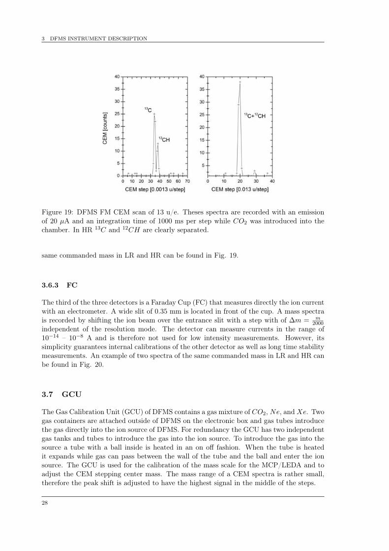
3 DFMS INSTRUMENT DESCRIPTION
Figure 19: DFMS FM CEM scan of 13 u/e. Theses spectra are recorded with an emissionof 20 µA and an integration time of 1000 ms per step while CO2 was introduced into thechamber. In HR 13C and 12CH are clearly separated.
same commanded mass in LR and HR can be found in Fig. 19.
3.6.3 FC
The third of the three detectors is a Faraday Cup (FC) that measures directly the ion currentwith an electrometer. A wide slit of 0.35 mm is located in front of the cup. A mass spectrais recorded by shifting the ion beam over the entrance slit with a step with of �m = m
2000independent of the resolution mode. The detector can measure currents in the range of10�14 – 10�8 A and is therefore not used for low intensity measurements. However, itssimplicity guarantees internal calibrations of the other detector as well as long time stabilitymeasurements. An example of two spectra of the same commanded mass in LR and HR canbe found in Fig. 20.
3.7 GCU
The Gas Calibration Unit (GCU) of DFMS contains a gas mixture of CO2, Ne, and Xe. Twogas containers are attached outside of DFMS on the electronic box and gas tubes introducethe gas directly into the ion source of DFMS. For redundancy the GCU has two independentgas tanks and tubes to introduce the gas into the ion source. To introduce the gas into thesource a tube with a ball inside is heated in an on off fashion. When the tube is heatedit expands while gas can pass between the wall of the tube and the ball and enter the ionsource. The GCU is used for the calibration of the mass scale for the MCP/LEDA and toadjust the CEM stepping center mass. The mass range of a CEM spectra is rather small,therefore the peak shift is adjusted to have the highest signal in the middle of the steps.
28

3 DFMS INSTRUMENT DESCRIPTION
Figure 20: DFMS FM Faraday cup scan of 28 u/e for HR (left) and LR. The step width forboth scans was 0.014 u/step. The emission was 200 µA and the integration time 1000 msper step.
3.8 DFMS operation
There exist rather large differences in the operation of DFMS FM and FS. The groundsupport equipment (GSE) for DFMS FM consists of a power supply simulating the 28 Vspacecraft bus and an ordinary computer with a special operating system (GSEOS). GSEOSsimulates the interaction between the operation center, the spacecraft and the DPU. Tooperate the instrument and detect ions on the detectors, many different voltages have to beadjusted and applied. The ion source voltages are set measurement mode dependent. Tomeasure ions the voltage set is different from the one used for neutrals. The voltage set forions and neutrals are stored in a table named ’Rositabs’ in the DPU memory. Other voltagesare resolution and mass dependent e.g. the slit region (ESS1 + ESS2) or the zoom voltages(ZQ1 and ZQ2). The voltages of the analyzer section are mass dependent (ESAI, ESAO,and Vaccel). The mass dependent voltages are calculated according to the mass that is to beanalyzed. The detector region has an other set of voltages that are signal dependent, likethe gain of the MCP (MCPFront). The gain is adapted automatically by an algorithm toadjust the signal on the LEDA. This gain adjust can be toggled on or off manually for theFM. All the voltage ranges are controlled by the DPU and error messages are implementedif the set voltage is not in the safety range. For DFMS FM all this voltages can be adaptedmanually or a spectrum of a certain mass (commanded mass) can be recorded, while thevoltages are set automatically. To reduce the commanding the DPU provides measurementmodes to command all this voltages automatically. The DFMS FS is mainly commanded inthis way for obvious reasons as the signal travel time or the workload during commissioning.Modes have the advantage that measurement sequences can be performed according to thescience questions to tackle or instrument calibrations. The modes can cover a mass rangeby commanding the masses according to the signal mass range on the detector. This massrange is then covered within a mode and contains several spectra. An other possibility isto record only specific masses in a mode, if one is interested in noble gases it is less time
29

3 DFMS INSTRUMENT DESCRIPTION
consuming to record spectra only of masses that are interesting (e.g. m/q 20, 40, 84, 132).The calibration modes with the GCU, are recorded in a similar fashion. Sets of modes canbe combined in sequences to simplify the planning of the operations.
3.9 Technical problems
Figure 21: Remote Detector Package (RDP): on the left side from top to bottom RDP-CON,RDP-FEM, RDP-DVI and RDP-FLI. On the right side the defect an later replaced inverteron the bottom side of the RDP-DVI board.
The detector package of DFMS is described in Sec. 3.6. Behind the detector package theRemote Detector electronics Pack (RDP) is located (for detailed documentation see Neefs etal. (2004)). The Remote Detector Package (RDP) consists of four boards (from the detectorpackage upwards): RDP-FLI, RDP-DVI, RDP-FEM and RDP-CON.After an arcing of the Vaccel, the MCP/LEDA rowB showed an unexpected behavior. Threeeffects are detectable (see Fig. 22): a drop in counts, a plateau and a ’memory’ effect. Thedrop in counts is in the first ⇠20 pixels. The plateau starting at a random pixel coversparts of rowB. The ’memory’ effect, shows some signal on the same pixels as the peak of theprevious taken spectrum.Several tests were performed in collaboration with BIRA and a possible damage of theLEDA or parts behind was localized. After the replacement of the LEDA, the three effectswere still detectable. By further inspection of the RDP electronics a tattered inverter onthe RDP-FLI was found and replaced. After this only the plateau effect is still randomlydetected and might be due to a timing problem during the switch on of the MCP.The new LEDA has a depleted signal on pixel 8 of rowB and an inflated signal on pixel 9.The same effect is seen on rowA for pixel 429 (inflated) and 430 (depleted). The effect mustbe taken in to account for the pixel gain evaluation.The Vaccel for DFMS FM and FS, was then limited to -6500 V, to avoid other technicalproblems.
30
3 DFMS INSTRUMENT DESCRIPTION
Figure 22: The three effects observed for rowB of LEDA for FM. The drop down in countscan be the first ⇠20 pixels, a plateau where a peak is seen for rowA and the ’memory’ effect.The ’memory’ effect, shows still some signal on the same pixels as the spectrum before thepeak was located.
31

3 DFMS INSTRUMENT DESCRIPTION
32

4 DFMS CHARACTERISTICS
4 DFMS characteristics
This chapter gives an overview of the data treatment and the characteristics of DFMS. In theion source the neutrals are bombarded with electrons, this can cause an instrument depen-dent characteristic fragmentation of molecules. How efficient a neutral is ionized depends onthe ionization cross section of the neutral, which depends on the bombarding electron energy.The transmission through the sensor is an instrument characteristic function, and takes intoaccount possible mass discrimination and the ion optical path through the instrument. Thedata evaluation of the different detectors is fundamental, and possible calibration functionsfor DFMS FM and FS are given. Corrections of the data especially for the MCP/LEDAdetector are given in the order of data treatment. The pixel gain and the recalibration ofthe MCP/LEDA gain polynomial are necessary correction factors for the data analysis ofthe MCP/LEDA. The results presented here are a continuation of earlier work and detectedproblems.
The sensitivity (S) of DFMS for the detection of a neutral species can be divided into threeparameters:
S / � · ⌧ · yield (15)
Where S is the sensitivity, � the ionization cross section, ⌧ the sensor transmission and yieldthe detection efficiency.The ionization cross section is species and electron energy dependent. For DFMS the elec-tron energy is nominal set to 45 eV (for detailed explanation see Schläppi (2011)) but canbe varied. The transmission through the sensor gives knowledge about how efficient ionsare guided through the sensor depending on their mass to charge ratio. For DFMS thetransmission is not the same for both resolutions since the flight path through the sensoris not the same. The detection efficiency is highly dependent on the type of detector. Forexample the impinging ion on the MCP/LEDA must have enough kinetic energy to releasesecondary electrons. The detection efficiency of the CEM and FC is not species dependentand therefore can be set to one.
4.1 Ion source
The ionization of neutrals in the ion source is an electron impact ionization. The energyof the electrons has an influence on the ionization efficiency and the fragmentation of aneutral. The electron bombardment of neutrals can cause fragmentation of the molecule,the distribution of the main molecule (parent) and the fragments depends on the moleculeand the electron energy, as well as the detection efficiency. It is therefore highly instrumentdependent.
4.1.1 Ionization cross section
The probability of a particle to get ionized by electron impact is proportional to the ion-ization cross section. Therefore, a particle is more likely to get ionized, if the ionizationcross section is bigger. The ionization cross section of a particle depends on the size of theparticle and the energy of the impacting electron. Furthermore the electron energy must behigh enough to ionize the neutral. The ionization energy for neutral atoms in the groundlevel is < 25 eV [Handbook of Chemistry and Physics, 2012]. The ionization efficiency has
33

4 DFMS CHARACTERISTICS
a rather typical maximum for an electron energy of 70 – 100 eV (see Fig. 23). However,this is not the case for DFMS, since the ion source geometry also has an influence on theionization efficiency and the maximum is at 45 eV (see Schläppi (2011)).
Figure 23: Ionization cross section of He, Ne and CO2 dependent on the electron energy.A maximum for the ionization cross section can be found for electron energies of 70 – 100eV. Data from Rice University (2013).
4.1.2 Fragmentation pattern
The fragmentation pattern of a molecule is an instrument dependent pattern. During theionization process (by electron impact ionization) not only the parent is ionized it also canfragment into fragments. The fragmentation pattern is highly dependent on the electronenergy. The fragmentation of the parent can be forced with higher electron energies. Thelower electron energies causes a higher amount of parents and simplifies the interpretationof a spectrum. The fragmentation pattern for CO2 measured with DFMS FM for differentelectron energies compared to NISTd can be found in Fig. 24. The fragmentation patternis the intensity of the parent (CO2) and the fragments (CO and O) relative to the sum ofthe intensity (CO2, CO, O and CO2 doubly charged). C is also a fragment of CO2 butsince the mass range detected by the MCP/LEDA does not cover this mass, the intensityof C is not taken into account. The fragmentation pattern for an electron energy of 45 eVdoes not fit the NIST values for 70 eV. A reason for this could be that the electron energyis reduced for DFMS, and therefore less fragmentation occurs. However the fragmentationpattern of NIST can neither be reproduced with an electron energy of 70 eV (see Fig. 24).
dThe data in NIST (http : //webbook.nist.gov/chemistry/) for the fragmentation pattern is given asnormalized intensities for the fragments or the parent. This intensity was then normalized to the total ofthe intensities.
34
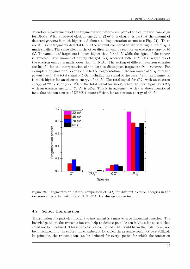
4 DFMS CHARACTERISTICS
Therefore measurements of the fragmentation pattern are part of the calibration campaignfor DFMS. With a reduced electron energy of 22 eV it is clearly visible that the amount ofdetected parents is much higher and almost no fragmentation occurs (see Fig. 24). Thereare still some fragments detectable but the amount compared to the total signal for CO2 ismuch smaller. The same effect in the other direction can be seen for an electron energy of 70eV. The amount of fragments is much higher than for 45 eV while the signal of the parentis depleted. The amount of doubly charged CO2 recorded with DFMS FM regardless ofthe electron energy is much lower than for NIST. The setting of different electron energiesare helpful for the interpretation of the data to distinguish fragments from parents. Forexample the signal for CO can be due to the fragmentation in the ion source of CO2 or of theparent itself. The total signal of CO2, including the signal of the parent and the fragments,is much higher for an electron energy of 45 eV. The total signal for CO2 with an electronenergy of 22 eV is only ⇠ 12% of the total signal for 45 eV, while the total signal for CO2
with an electron energy of 70 eV is 36%. This is in agreement with the above mentionedfact, that the ion source of DFMS is more efficient for an electron energy of 45 eV.
Figure 24: Fragmentation pattern comparison of CO2 for different electron energies in theion source, recorded with the MCP/LEDA. For discussion see text.
4.2 Sensor transmission
Transmission of a particle through the instrument is a mass/charge dependent function. Theknowledge about the transmission can help to deduce possible sensitivities for species thatcould not be measured. This is the case for compounds that could harm the instrument, notbe introduced into the calibration chamber, or for which the pressure could not be stabilized.In principle, the transmission can be deduced for every species for which the ionization
35

4 DFMS CHARACTERISTICS
cross section, the fragmentation behavior, the sensitivity and the detection efficiency ofthe detector is known (according to Equ. 15). However, the fragmentation behavior ofDFMS is part of the calibration campaign and can therefore not be assumed to be wellknown. This leaves the noble gases as candidates to deduce the sensor transmission, sincenoble gases do not fragment and the ionization cross section is well known for differentelectron energies. To avoid uncertainties of the detection efficiency the transmission of theinstrument was deduced from CEM measurements. The sensor transmission of DFMS can
Table 7: The ionization cross section for noble gases for an ionization energy of 45 eV[Rice University, 2013].
Species Ionization cross section [10�17 cm2] Correction factor relative to Ar
Ne 2.5 0.10Ar 24.9 1.00Kr 33.8 1.36Xe 46 1.86
be deduced from the sensitivity measurements of the noble gases (for a detailed descriptionof the sensitivity measurements see Sec. 5.4). The sensitivities of the noble gases are thencorrected for the different ionization cross sections for an ionization energy of 45 eV relativeto Ar. The correction factors for the different noble gases can be found in Tab. 7. Sincethe ion path through the sensor is resolution dependent, the transmission function is givenfor both resolutions independently.
⌧HR(m) = aHR ·m�1.135 (16)
⌧LR(m) = aLR ·m�0.853 (17)
⌧HR is the transmission of the instrument for HR and ⌧LR for LR.The transmission function has an emission and resolution dependent correction factor a,while m is the mass to charge ratio of the species.It is known from previous measurements that the sensitivity for an emission current of 200µA is slightly lower than for the other emissions. This can be explained by the higher spacecharge around the filament, that widens up the electron beam and the ratio of electronsreaching the ionization region is lower compared to the other emissions. To account forthis process the correction factor ai for the transmission is slightly lower for 200 µA. Thecorrection factor ai for all emissions and both resolutions can be found in Tab. 8.
Table 8: The correction factors ai for ⌧ for all emissions and both resolutions.
Emission HR/LR ai for ⌧
2 and 20 µA LR 3.126 x 10�16
200 µA LR 1.304 x 10�16
2 and 20 µA HR 8.411 x 10�17
200 µA HR 2.147 x 10�17
The sensor transmission should be the same for FS and FM. However, the sensitivity for theFS for 200 µA is known to be higher than for the other emissions. This is documented in
36

4 DFMS CHARACTERISTICS
several memos about the sensitivity of GCU measurements (see Eberhardt (2008a), Altwegg(2008a), Eberhardt (2008b), and Altwegg (2008b)). A possible explanation could be thatthe ion source geometry is slightly different for the FS and the electrons are guided moreefficient into the ionization region than for the FS. Therefore the correction factors ai of theFM for an emission of 200 µA should be adapted for the FS.
4.3 MCP/LEDA data
The MCP/LEDA is the main detector of DFMS. It consists of MCP and LEDA of twoindependent rows each with a pixel number of 512. To derive the ion current per spectrumfor one species i the following steps have to be taken into account:
1. Subtract offset for both rows individually
2. Correct for individual pixel gain for both rows separately
3. Apply mass scale for both rows individually
4. Sum of the peak of species i for both rows together (Sumi)
5. Correct for MCPGain
6. Calculate ion current (IMCP,i) for species i
IMCP,i =Sumi · cadc · cleda
MCPGain · t (18)
Where cadc =2.5V212�1 is the conversion factor of the 12 bit LEDA analog to digital converter
and cleda = 4.22 · 10�12 F the anode capacity and divided by the total integration time t(nominal t = 66 ms · 300 = 19.8 s). The ion current IMCP,i is then in A.For calibration purposes as well as for the evaluation of the statistical error the number ofions per spectrum is useful and defined as:
ni =IMCP,i · t
q(19)
where ni is the number of ions of species i per spectrum, IMCP,i is the ion current, t thetotal integration time and q the elementary charge.The statistical error in % of IMCP,i is therefore
�ni =1
pni
· 100 (20)
The above mentioned steps to derive the ion current per spectrum are discussed step by stepin the following chapters. The applied corrections for the FM are used during calibration inChapter 5) and possible approaches for the FS are mentioned.
37

4 DFMS CHARACTERISTICS
4.3.1 Offset correction
Before a spectrum is recorded on the LEDA, an amount of charge is applied on both rowsof the LEDA. The amount of applied charge depends on the accumulation number of aspectrum, since each time before the LEDA starts to record, the same charge is applied.The nominal integration time and accumulation number is 66 ms and 300. The offset due tothe accumulated charge during the recording process of one spectrum, has to be subtractedfrom the counts in a spectrum. To determine the offset function (Oi), the signal of the peakis cut out, and the remaining counts are then fitted. This has to be done individually forboth rows since the applied charge is not the same for both rows. The reason for this couldbe a slightly different resistance for each row. However, since the amount of charge and theresistance are the same for all recorded spectra of the FM the function of the offset staysthe same.
OFMrowA = �2 · 10�6p3 + 0.0017p2 � 0.5268p+ 4091.1� dA (21)
OFMrowB = �1 · 10�6p3 + 0.0013p2 � 0.5058p+ 3363.2� dB (22)
While p is the pixel number, dA and dB are adjusted individually for each spectrum toreduce the number of counts to a level of ± 5 counts per pixel, for pixels where no peak isfound. The signal of the spectrum in counts is then reduced to a few counts, where no peakis detected, while the counts of the peak is reduced by the offset (see Fig. 25).
Figure 25: The offset subtraction in principle for rowA.
The correction of the offset for the FS can be done similar to the FM:
OFSrowA = �3 · 10�6p3 + 0.0022p2 � 0.5290p+ 4771 + dA (23)
OFSrowB = �2 · 10�6p3 + 0.0015p2 � 0.249p+ 5530 + dB (24)
Differences between FM and FS can be explained by the slightly different resistances of theLEDA.
38

4 DFMS CHARACTERISTICS
4.3.2 Individual pixel gain
Figure 26: Picture of an MCP with the hexagonal structure due to fabrication fashion. Thestructure causes a modulation in the individual pixel gain of 24 pixels for the FM.
The pixel gain is a correction factor for every individual pixel to correct for the degradationof the MCP over time. The degradation of the MCP is due to an uneven ion currentimpinging on the area of the MCP. The ion optics focuses the main ion current in such away on the MCP, that the commanded mass is in the middle of the MCP. Since therefore,most ions impinge in the middle of the MCP, most electrons are emitted there, resulting inan depletion of the MCP center.The following proceeding for the measurement of the individual pixel gain correction is asummery of the work of Riesen (2007) and Schläppi (2011). This depletion of the MCPis first mentioned and corrected by Riesen (2007), and is expected and well understood.Measurements for the pixel gain correction are performed and analyzed in the followingway:
• A narrow peak (LR) is shifted with a step width of 4 pixels over the whole MCP/LEDAby commanding slightly different masses. The range of the commanded masses is givenby the mass range of one spectrum. �m is then calculated according to the mass rangeof 4 pixels. For example if the peak is H2O, the mass range is 17.05 u/e – 18.98 u/e,�m = 0.0145 and a total of 134 spectra is recorded. The detector gain of the MCPhas to remain the same during recording. Therefore the gain algorithm that calculatedthe detector gain according to the intensity of the peak, has to be switched off oncethe detector gain is adjusted for the peak to be shifted.
• To calculate the pixel gain correction factors, the intensities of the peaks relative tothe pixel are added and scaled to the average of pixel 20 to 492 to avoid border effectsof the MCP/LEDA. The dimensionless correction factors are then in the range of ⇠0.4– 1.5. A correction factor of 1.0 means that the intensity of the peak recorded for thispixel is exactly the average of the other intensities.
The commanding of the different masses can be done within a measurement mode for H2O,on the detector gain adjusted by the gain algorithm for the intensity of the H2O peak (FM
39

4 DFMS CHARACTERISTICS
and FS). An other possibility for the FM is to use a batch wherein, the species and the gainstep can be adapted (integration time is 6.6 s). The shift in pixels is optimized for recordingtime and modulation effects of the step width overlaying the known modulation of the MCPwith a step width of 24 pixels for the FM.The modulation of the pixel gain of the MCP for the FM is well known and due to thefabrication of the MCP. A picture of a MCP fabricated in a similar fashion as for the FMcan be found in Fig. 26. The fabrication of the MCP for the FS was different to avoid thismodulation.
Figure 27: FM individual pixel gain of rowA and rowB of the same species on the sameMCPFront (GS=14). To distinguish the two rows, rowB is plotted with an offset of 0.1. Noreliable corrections are given for the edges of the MCP, due to data processing.
The proceeding of the spectra is done separately for rowA and rowB. RowA and rowB aretreated separately since the ion beam is not always perfectly focused in the middle of theMCP. However the variation between the two rows is marginal (see Fig. 27).To apply the correction of the individual pixel gain on a spectrum, the number of countsfor every individual pixel is divided by the correction factor of the specific pixel of rowA orrowB for the recorded MCPGain of the spectrum.Since the peak in the middle of the LEDA is no longer amplified in the same amount (can beless than 50% of the nominal amplification) through the MCP, the correction factor there isthe lowest one. The correction factor is not dependent on the species of the peak but highlydependent on the gain step or the difference of MCPFront �MCPBack (see Riesen (2007)and Schläppi (2011)). A specific difference between MCPFront � MCPBack is called gainstep (GS). The highest gain is GS 16 and has a �(MCPFront �MCPBack) of -2300 V, thelowest gain has GS 1 and �(MCPFront �MCPBack) is -1300 V.For a successful and correct recording of the individual pixel gain for one GS (duration 2h) a highly stable density of the recorded species around the instrument is necessary. Thisrequires a regulated pressure (if additional gas is introduced into the chamber) and a tem-perature stable instrument and environment. The intensity of the ion beam that is shiftedover the MCP should be stable, therefore variations of the density around the instrumentand in the chamber should be limited. To get a stable environment for the FS the variations
40

4 DFMS CHARACTERISTICS
Figure 28: FM individual pixel gain of row A on gain step 7 to 14.
of the densities around the instrument due to spacecraft outgassing [Schläppi et al., 2010]have to be limited.A set of the recorded individual pixel gain for the FM can be found in Fig. 28. The recordingis part of the calibration measurements and the resulting correction factors are applied duringanalysis. The set was recorded with the above mentioned batch on several species. GS 16 to11 was recorded with a peak of the background gas, and different emissions. GS 10–7 wasrecorded with additional CO2-gas introduced into the chamber with a regulated pressureinlet. To have a stable background density the instrument was running at least 2 h beforestarting the measurements of the individual pixel gain.
Figure 29: FM comparison of pixel gain recorded in 2009 and 2012, with a depletion in themiddle of the MCP of ⇠40%.
41

4 DFMS CHARACTERISTICS
Comparison of the individual pixel gains of FM in Schläppi (2011) and the new recorded ones,show a further depletion of the MCP in the center of ⇠40% (see Fig. 29). A further depletionwas expected since the measurements recorded with the MCP were proceeding. Betweenthe two measurements are ⇠3000 h of MCP operation or 3 years of intense measurementperiod. The recording of a set of the individual pixel gain for the FM as well as for the FSshould therefore be done on a regular time basis depending on the MCP operation time.For the FS a measurement set every 3–4 month is therefore recommended.
4.3.3 Applying the mass scale
The most difficult and critical step is to apply the mass scale. In this step the pixel numbersare translated into mass to charge ratios. A shift of several pixels can lead to completelydifferent interpretations according to the species that caused the spectrum. While for m/q= 13 u/e there exists only tow species that can cause a peak on this spectrum (13C andCH), for m/q = 19 u/e much more possibilities exist and the peak of fluorine might bewrongly interpreted as 18OH (a shift of 15 pixels). Therefore this step has to be done verycareful. The mass of a spectra according to the pixel number can be calculated as:
m(p) = m0 · e(p�p0)x
D·z (25)
Where m(p) is the mass to charge ratio that falls on this specific pixel p, which is the pixelnumber (1 p 512). p0 is the pixel where the commanded mass m0 is located and x isthe step width between two pixels (x = 25 µm). D is the dispersion factor (D = 127’000µm [Wüthrich, 2007]) and z is the zoom factor (LR: z = 1 and HR: z = ⇠ 6.4)In an ideal case of a perfectly adjusted instrument, the ion optical axis of the sensor intersectsthe focal plane of the MCP/LEDA. The commanded mass m0 of a spectrum should thereforebe in the center of the MCP/LEDA, on pixel 256, and both rows should record exactly thesame signal (after subtraction of the offset). In general this is true and the consequencethereof is the depletion of the MCP in the middle section. However, the commanded massm0 is not always on pixel 256 but falls on pixel zero (p0). In LR this has a much smallereffect since the resolution between tow pixels is much smaller than in HR (�m/pixel / e
1z ).
For FM shifts of ⇠± 50 pixels for p0 are detected during the calibration campaign for HR.The GCU spectra are important to calibrate p0 since the expected species (Ne, CO2 andXe) are known and therefore the according p0 for spectra wherein these species are found.However, the GCU spectra give only limited information about p0, compared to the totalmass range. An other phenomenon is a shift of p0 for m0 � 70 u/e in HR, due to the appliedpost acceleration (PA = -1 kV). The function of p0 for HR is divided into three parts (seeEq. 26, 27 and 28), to account for the different zoom values (see Tab. 9), since a correctionof the zoom value can also cause a shift of p0. The calculated p0 according to Eq. 26, 27,and 28 for HR should fit for the first and second order segment of the variable m0 within ±2 pixels, while the zero order segment (offset) of the function might change with time dueto temperature influences of the magnet.
p0(m0) = �0.3958m20 + 15.169m0 + 165.03 13 m0 < 22 (26)
p0(m0) = �0.0101m20 + 0.7971m0 + 290.8 22 m0 < 70 (27)
p0(m0) = �0.498m0 + 335.25 70 m0 100 (28)
42

4 DFMS CHARACTERISTICS
The function of p0 for LR is a linear function (see Eq. 29), since the number of pixels betweentwo masses is a linear function for the commanded mass. This function is also stronglytemperature dependent since the pixel, where the commanded mass impinges depends onthe radius of the ion path through the magnet and therefore the temperature.
p0(m0) = �0.0747m0 + 266.46 13 m0 136 (29)
The calculated p0 according to Eq. 29 for LR should fit for the first and second ordersegment of the variable m0 within ± 2 pixels, while the zero order segment (offset) of thefunction might change with time due to temperature influences of the magnet.The dispersion factor of the MCP/LEDA is well known [Wüthrich, 2007]. All the detectorpotentials are floating on Vaccel and only this potential is mass dependent, all the other po-tential differences are constant. This effect is well understood and documented in Wüthrich(2007) and Riesen (2007). Therefore the dispersion factor is a constant over the total massrange since the distribution of the ion beam over the MCP/LEDA is dependent on thepotential differences of the detector.The zoom factor is constantly one for LR since the zoom optics are not applied in thismeasurement mode. For HR the zoom factor is nominal 6.4 but because of a recalibrationof the mass dependent voltages applied on the zoom quadrupoles, for m0 20 u/e, thezoom factor is in the range of 5 z 6.6 (see Tab. 9). To account for the applied postacceleration and resulting concentration of the peaks on the LEDA, the zoom factor for m0
� 70 u/e is much smaller than the nominal 6.4 (see Tab. 9).
Table 9: Zoom values for HR for DFMS FM
m0 z [± 0.2] m0 z [± 0.2]13 5.8 21–69 6.414 5.3 78 3.815 6.0 80 3.816 6.3 82 3.817 6.4 83 3.818 6.3 84 3.819 6.6 86 3.820 6.2
4.3.4 MCP/LEDA gain polynomial
The MCP/LEDA gain polynomial describes the amplification of the signal through theMCP. If an ion impinges on the MCP, a cascade of electrons is released and detected onthe LEDA. To interpret the number of counts into the number of ions that impinged on theMCP, the gain of the MCP has to be known (see Eg. 30). The gain of the MCP is describedas a function depending on the potential difference of the MCP (MCPFront �MCPBack).A specific difference between MCPFront �MCPBack is called gain step (GS). The highestgain for FM is GS 16 and has a �(MCPFront �MCPBack) of -2300 V, the lowest gain hasGS 1 and �(MCPFront �MCPBack) is -1300 V.
Gain =#ions
#electrons(30)
43

4 DFMS CHARACTERISTICS
The calibration of the gain polynomial was first performed during the detector calibration.These measurements were done for the FM and the FS only with the detector in the cali-bration chamber (FM: Nevejans et al. (2001) and FS: Neefs et al. (2002)). A refitting of thegain polynomial was done during the pre flight calibration campaign (FM: Langer (2003a)and FS: Langer (2003b)). However during the calibration of DFMS FM by Riesen (2007),a correction factor for the gain was applied to compare measurements of different GS. Toavoid this correction factor the gain polynomial was re calibrated for this work.
MCPGain =IionIleda
(31)
Where Iion are the number of ions that impinge on the MCP and Ileda is the signal measuredon the LEDA. Typically the gain of a two stack MCP with the above mentioned configurationand dimensions is in the range of ⇠ 106 at an applied voltage of -2 kV.The measurement setup was the same as for the measurements of the individual pixel gain.For high GS the signal of the background gas was used while for lower GS additional gas(CO2) was let into the chamber. Spectra in LR of the commanded mass 16, 18, 20, 34 and44 are measured on the nominal GS for the signal. Then the GS was manually adapted (± 1GS) and a spectrum was recorded. The factor between two gain steps is given by the ratio ofthe peak areas at the corresponding gain steps. To avoid pixel gain corrections, the highestsignal of the peak is manually shifted to the same pixel. If several measurements were donefor the same gain steps the average of the ratio between two measurements was taken. Thestatistical error is the standard deviation of the average. For the total uncertainties of 6%the statistical error of the single measurements < 3% as well as uncertainties of the average< 5% are taken into account.
Table 10: MCP/LEDA Gain TableGainstep Gain FM old⇤ MCPFront �MCPBack[V ] Gain FM refitted+
1 4.94E-02 -1300 1.41E-012 2.62E-01 -1342 3.88E-013 1.16E+00 -1382 1.01E+004 5.11E+00 -1425 2.79E+005 2.02E+01 -1468 7.63E+006 7.82E+01 -1514 2.20E+017 2.84E+02 -1562 6.48E+018 9.64E+02 -1612 1.94E+029 3.09E+03 -1665 5.97E+0210 9.40E+03 -1722 1.90E+0311 2.76E+04 -1785 6.41E+0312 7.73E+04 -1855 2.25E+0413 2.01E+05 -1932 7.84E+0414 5.19E+05 -2025 2.89E+0515 1.34E+06 -2140 1.02E+0616 3.97E+06 -2300 2.78E+06
⇤[Langer, 2003a] + in this work
Two gain ratios (1-2 and 2-3) were not measured, because no signal could be detected for apressure of ⇠ 5 x 10�7 mbar. Therefore they were extrapolated from the gain polynomial,
44

4 DFMS CHARACTERISTICS
which fits the detector gains for the gain steps 3 to 16. However, the physical interpretationof a gain < 1 is not understood by the author and measurements are not likely to beperformed on this gain steps. The absolute calibration of GS 16 was done with single ionmeasurements. The pressure level was adjusted so that the number of ions impinging on theMCP within one spectrum (2 s) were limited to one. The resulting signal on the LEDA, wasthen interpreted as the gain for one ion. The average of the 100 single ion measurements thengives the start point of the gain polynomial at gain step 16. Because of the uncertaintiesdue to statistics the total error (10%) for this point is slightly higher than for the othermeasurements (see Fig. 30), however total uncertainties are smaller than symbol size.The calculated gain polynomial is the following:
MCPGain(x) = 102.36·10�9x3+8.33·10�6x2�9.26·10�4x�10.95 (32)
Whereas x is MCPFront � MCPBack voltage. The measured gain is not comparable tothe old measurements within error bars therefore the gain polynomial was refitted. Anexplanation could possibly be found in the different measurement setup. In the first setuponly the detector was used for calibration and now the whole sensor. Another reason couldbe the decreasing of the MCP’s efficiency due to aging.Isotopic measurements of the D/H ratio for Water in LR of H2O and HD18O imply highaccuracy for the refitted gain polynomial (for further detail see Sec. 5.5). The ratio ismeasured, covering seven gain step and fits the literature value within error bars.
Figure 30: MCP gain for DFMS FM. The ’old’ gain are the gain values from the firstcalibration [Langer, 2003a] and ’new’ gain are the values of the calibration in this work.
45

4 DFMS CHARACTERISTICS
4.4 CEM data
To evaluate CEM data, the calculation of the ion current for the CEM is described andthe mass shift between two steps to calculate the mass scale. The CEM detector is mainlyoperated in digital mode, where CEM operates in a constant high gain plateau at a frontvoltage of – 2337 V. The repetition voltage in the CEM is – 100 V. In this mode events arecounted, more precisely the arrival of a secondary electron cloud, caused by an impactingion. The saturation limit for counting is around 2 · 106 events per second. A spectrum ofthe CEM detector is recorded by shifting the ion beam in little mass steps over the entranceslit of the CEM detector. The nominal integration time per step is 1000 ms and the numberof steps is mass and resolution dependent.
Table 11: CEM mass step width and number of steps per spectrum
Step width Number of steps
Low resolution �m = m1000 ⇠ 140p
m+ 1
High resolution �m = m10000 ⇠ 240p
m+ 1
The shifting of the ion beam over the entrance of the CEM causes an overlap of the ionbeam. The overlap is calculated the following:
col =D�m
m
ws(33)
Where D is the dispersion (127’000 µm), �mm is the step width and ws is the width of the
entrance slit of 25 µm. The overlap correction factor for LR is col = 5.08 and col = 0.508for HR.The ion current of a species i (ICEM,i) of the CEM detector operated in digital mode iscalculated the following:
ICEM,i =col · Sumi
t(34)
The Sumi is the sum of the peak of species i and t is the integration time per step (nominal1 s). The statistical error of the CEM is calculated in the same way as for the MCP/LEDAin Eq. 19 and 20.
4.5 FC data
To evaluate FC data, the calculation of the ion current for the FC is described. The FChas an entry slit width of 0.35 mm which is big compared to the beam width (⇠0.25 mm)in high resolution mode and comparable to the beam width (⇠0.357 mm) in low resolutionmode. While stepping the ion beam over the detector entrance of the FC, the ion beamwill always reach a position where the whole beam passes into the detector unhindered.Therefore, the amplitude of the peak is used for ion current calculations. The FC step sizeis not resolution dependent nor the number of steps:
46

4 DFMS CHARACTERISTICS
�m =m
2000(35)
m is the commanded mass and the number of steps is then ⇠ 240pm+1. The integration time
t per step is 1 s. The Faraday Cup is a simple detector with only an electrometer at its end.A spectrum consists of the measured electrometer output per step which is provided in theunit mV .The ion current of species i (IFC,i) of the FC detector is calculated the following:
IFC,i =cel · Vmax,i
t(36)
Where Vmax,i is the amplitude of the peak of species i, cel is the correction constant totransfer the measured voltage into the corresponding current.
cel = 3.33 · 10�15
A
mV
�(37)
The statistical error of the FC is calculated in the same way as for the MCP/LEDA in Eq.19 and 20.
4.6 Sensitivity
The sensitivity of a sensor for one species is the detected particles (atom or molecule) relativeto that available. To detect a particle it has first to be ionized, where fragmentation canoccur, then guided through the sensor and finally detected. The sensitivity of DFMS forspecies i is defined as the total signal (current) detected for the species relative to the densityof the species and the emission:
Stotal,i =Iion⇢Iemi
(38)
While Stotal,i is in cm3, Iemi is the emission current in A and ⇢ is the density in cm�3. Iionis the current detected for i. The total signal contains the signal due to the parent, thefragments, the isotopes and the doubly charged particles. To transform the signal into thecorresponding ion current, the data is proceeded as described in Sec. 4.3, 4.4, and 4.5.Unfortunately the densities are usually measured as pressures, although a current and there-fore a density is measured and correction factors for different species have to be applied.The relation between density (⇢) and pressure (p) in a specific volume is given by:
pV = NkBT ) ⇢ =N
V=
p
kBT(39)
While p is the pressure in Pa, V is the volume in cm3, N is the number of particles, kB isthe Boltzmann constant (1.38 x 10�23 J/K) and T is the temperature in K.To calculate the density for a specific pressure, a room temperature of 293 K was used inthe lab.The sensitivities of the CEM and the FC for one species should be comparable within un-certainties since both detectors measure a current. The difference between the MCP/LEDAand the CEM in sensitivity is the relative detection efficiency (yield). The detection effi-ciency of the MCP/LEDA depends strongly on the released electrons of the MCP when anion impinges on the MCP. The yield of a micro channel plate can be calculated (see Meier
47

4 DFMS CHARACTERISTICS
and Eberhardt (1993)), however the calibration for this calculation was performed with asimilar micro channel plate configuration but with much higher gains, and as discovered dur-ing calibration the values might not fit necessarily for the MCP/LEDA setting of DFMS.A factor of ⇠14 between the sensitivity for low and high resolution can be explained by theresolution dependent slit area (200 µm / 14 µm = 14.3), however this is no longer true whenpost acceleration is applied in HR. Nevertheless the transmission through the sensor is alsoresolution dependent and therefore the factor between LR and HR can vary. However theknowledge about this corrections might help to estimate the sensitivity for species, that arenot applicable for calibration measurements, because this species can harm the instrument,the chamber or are poisonous.
48

5 CALIBRATION OF DFMS IN A STATIC ENVIRONMENT
5 Calibration of DFMS in a static environment
To understand and interpret data of ROSINA at the comet, the sensors have to be cali-brated in an environment similar to that of the comet. Therefore the testing environmentCASYMIR (CAlibration SYstem for the Mass spectrometer Instrument ROSINA) was de-signed for this purpose. The calibration of DFMS describes the sensitivity of the instrumentfor different species, the fragmentation behavior of the ion source, the capability to measureisotopic ratios, and the relation of the signal of the instrument relative to different densitiesof the environment. To simulate the different velocities of neutrals relative to the instru-ment, CASYMIR can be operated in two modes: static and dynamic. In the static modethe velocity distribution of the neutrals is thermal and the same for every direction. In thedynamic mode the neutrals have a velocity in one direction. Both sensors FM and FS werecalibrated within a calibration campaign with a limited number of gases (CO2, Ne, Xe, andthe GCU-gas, that is a mixture of the three) [Langer et al., 2003]. The further calibrationof the FM for several species is key to understand and interpret the measurements at thecomet. The first calibration campaign for neutral species after launch can be found in Riesen(2007). The calibration therein was performed in a static and dynamic mode for CO2, Ne,Kr, and Xe.The calibration is focused on the following measurements: sensitivity of the instrument fordifferent species, fragmentation behavior of the ion source, and ability to measure isotopicratios. The calibration campaign presented in this work was performed for the followingspecies:
Table 12: The gases used for calibration of DFMS FM.
Species Description Purity⇤ [%] Remark e.g.Ne Neon 99.9998 [Bockelée-Morvan et al., 2004]Ar Argon 99.9998 [Bockelée-Morvan et al., 2004]Kr Krypton 99.9998 [Bockelée-Morvan et al., 2004]Xe Xenon 99.9998 [Bockelée-Morvan et al., 2004]H2O Water distilled [Hartogh et al., 2011]N2 Nitrogen 99.9998 [Bockelée-Morvan et al., 2004]CO2 Carbon dioxide 99.9998 [Bockelée-Morvan et al., 2004]CH4 Methane 99.9998 [Bockelée-Morvan et al., 2004]C2H6 Ethane 99.9998 [Bockelée-Morvan et al., 2004]C3H8 Propane 99.9998 [Schläppi et al., 2010]C4H10 n-Butane 99.9998 [Schläppi et al., 2010]C2H4 Ethylene 99.9998 [Bockelée-Morvan et al., 2004]⇤ purity is given by gas company
5.1 Calibration facility (CASYMIR)
CASYMIR was designed for the calibration of the ROSINA instruments in 1997 – 2000and further updated during subsequent measurement campaigns. A detailed description ofthe assembly of CASYMIR and the diagnostic tools can be found in Westermann (2000).CASYMIR is designed to simulate the atmospheric conditions in the vicinity of the cometsnucleus. It is designed in a multi staged vacuum chamber system to allow calibration at very
49
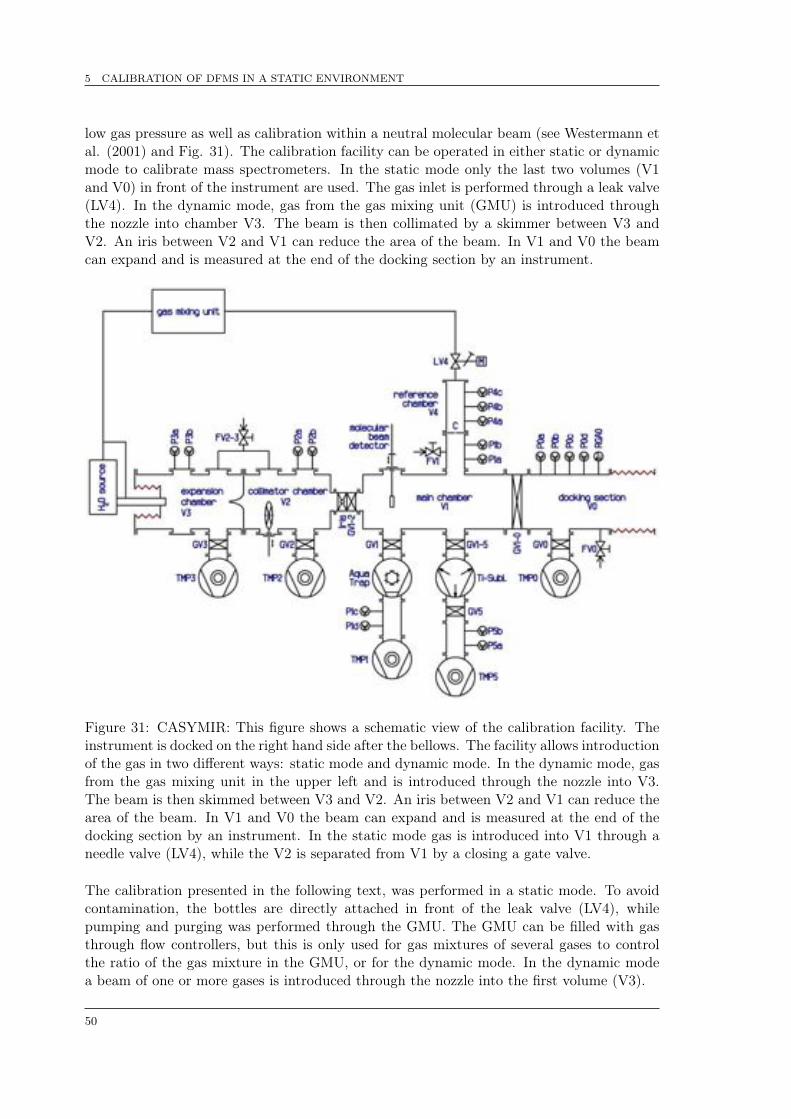
5 CALIBRATION OF DFMS IN A STATIC ENVIRONMENT
low gas pressure as well as calibration within a neutral molecular beam (see Westermann etal. (2001) and Fig. 31). The calibration facility can be operated in either static or dynamicmode to calibrate mass spectrometers. In the static mode only the last two volumes (V1and V0) in front of the instrument are used. The gas inlet is performed through a leak valve(LV4). In the dynamic mode, gas from the gas mixing unit (GMU) is introduced throughthe nozzle into chamber V3. The beam is then collimated by a skimmer between V3 andV2. An iris between V2 and V1 can reduce the area of the beam. In V1 and V0 the beamcan expand and is measured at the end of the docking section by an instrument.
Figure 31: CASYMIR: This figure shows a schematic view of the calibration facility. Theinstrument is docked on the right hand side after the bellows. The facility allows introductionof the gas in two different ways: static mode and dynamic mode. In the dynamic mode, gasfrom the gas mixing unit in the upper left and is introduced through the nozzle into V3.The beam is then skimmed between V3 and V2. An iris between V2 and V1 can reduce thearea of the beam. In V1 and V0 the beam can expand and is measured at the end of thedocking section by an instrument. In the static mode gas is introduced into V1 through aneedle valve (LV4), while the V2 is separated from V1 by a closing a gate valve.
The calibration presented in the following text, was performed in a static mode. To avoidcontamination, the bottles are directly attached in front of the leak valve (LV4), whilepumping and purging was performed through the GMU. The GMU can be filled with gasthrough flow controllers, but this is only used for gas mixtures of several gases to controlthe ratio of the gas mixture in the GMU, or for the dynamic mode. In the dynamic modea beam of one or more gases is introduced through the nozzle into the first volume (V3).
50

5 CALIBRATION OF DFMS IN A STATIC ENVIRONMENT
5.2 Measurement procedure
The calibration contains measurements for all three detectors (MCP/LEDA, CEM, FC) atall three emission settings (2 µA, 20 µA, 200 µA) in both resolution modes (LR and HR). Tomeasure the pressure as close as possible to DFMS an additional Granville-Phillips ion gaugewas installed in the flange where DFMS is attached to the calibration system. The calibrationwas performed in the most thermal and pressure stable or stabilized environmente. Toperform the calibration measurements the following procedure was used:
1. The instrument was running in a thermally stable environment while measurementswere performed. Therefore the instrument was running at least 1.5 h before the cali-bration measurements started.
2. Background measurements of the residual gas in the chamber were performed beforethe calibration gas was introduced into the chamber.
3. The calibration gas inlet was stabilized and controlled with a thermal valve. Thecalibration measurements were done after a stabilization time of > 0.5 h, although thepressure was already at a stable level before this time.
4. The same measurements were performed for every calibration gas while the samespectra were measured at the beginning of calibration as well as at the end.
The measurements of two gases (Ne and Ar) at the beginning of the calibration campaignwere performed on different pressure levels to find a correlation between the density in thechamber and the recorded signal. Once the correlation was found to be linear the rest ofthe measurements were performed at one pressure level.
5.3 Data treatment
Proper evaluation of the measurements is an essential part of the calibration. To transferthe signal detected into an ion current, the steps for the different detectors (MCP/LEDAin Sec. 4.3, CEM in Sec. 4.4 and FC in Sec. 4.5) were followed as previous described. Thesensitivities, fragmentation pattern, and isotopic ratios are calculated:
• SensitivitiesThe sensitivities were calculated according to Eq. 15. The pressure measurementswere corrected for the Granville-Phillips ion gauge. Correction factors can be foundin App. F.
• Fragmentation patternThe fragmentation pattern is the ratio of the intensities of each mass peak belonging tothe species relative to their cumulative intensities and is a dimensionless number. Forexample the fragmentation pattern of H2O is calculated by dividing the ion currentsof O, OH and H2O by the total of the three. As reference the fragmentation patternfor the same molecule in NIST is given although it is known that the electron energiesare not the same. Tables of the fragmentation pattern for each gas can be found inApp. E.
eThe calibration in a absolute static environment (no pumps and no gas inlet during measurements) wasnot feasible, because of sensor protection.
51

5 CALIBRATION OF DFMS IN A STATIC ENVIRONMENT
• Isotopic ratiosThe isotopic ratios were calculated by dividing the ion currents measured for theisotope divided by the ion current for the most abundant isotope. The relative isotopicabundances given in literature for Earth [Handbook of Chemistry and Physics, 2012]were then treated in the same way. For comparison the measured value has beendivided by the literature value. A value of exactly one indicates that the measurementis in total agreement with the literature value.
5.4 Noble Gases
In the following a summary about remote sensing measurements of noble gases is given[Bockelée-Morvan et al., 2004]: The noble gases (He, Ne, Ar, Kr, Xe, Ra) are highlyvolatile and chemically inert. The abundances of noble gases in the cometary nuclei as wellas in the coma are potentially diagnostic for the role played by cometary bombardmenton the formation and evolution of planetary atmospheres. Noble gas abundances are alsokey indicators of the temperature conditions and condensation processes in the outer solarnebula. The abundances of noble gases in a comet’s nuclei are diagnostic of the thermalhistory of the comet. Remote observations of the noble gases are difficult to perform becausetheir resonance transitions lie in the far-UV (� 1200 Å) spectral region. Only space bornobservations can access these wavelength. The detection of He does not help to solve theriddle about the thermal history of the comet but can be used as probes of the solar windconditions and of the interaction between cometary nuclei and the evidence of solar wind.However the detection of He in the coma of comet 67P/Churyumov-Gerasimenko is notpossible for DFMS since the mass range is limited to 12 u/e. Several upper limits can befound for Ne/O , while a depletion of 25-2600 relative to the solar value could be detected(25: Krasnopolsyk et al. (1997), 2600: Krasnopolsky and Mumma (2001)). The detection ofArgon with remote sensing is difficult because of the confusion of Ar with other spectral linesat low resolution, therefore the detection of Ar in comet Hale-Bopp is questionable. Thesearch for noble gases has been attempted by several space born observations but there hasnot yet been a convincing detection of any noble gas sublimation from a cometary nucleus[Bockelée-Morvan et al., 2004]. Therefore the detection of noble gases in cometary nuclei isquestionable and difficult. DFMS will provides the best circumstances yet for the detectionof noble gases due to its sensitivity and mass resolution. Therefore it is likely that DFMSwill provide the first conclusive measurements of noble gases in the comet’s coma.
52

5 CALIBRATION OF DFMS IN A STATIC ENVIRONMENT
5.4.1 Ne Neon
The detection of Ne at comets has been questionable although upper limits have beendeduced from space born measurements. However Ne was chosen as a component of theGCU-gas of DFMS and therefore used for calibration. The calibration measurements wereperformed at three different pressure levels: 2 x 10�8 mbar, 2 x 10�7 mbar, and 4 x 10�7 mbarcorrected for Ne (for correction factor see App. F). Special calibration modes exist for theFM to measure 20Ne and 22Ne for each detector and all emissions. These modes were usedduring calibration, therefore the ratio of 21Ne to 20Ne was not measured. However isotopicmeasurements for this ratio can be found in Riesen (2007) which are in good agreement withliterature. The background pressure before calibration measurements was at the level of ⇠1x 10�9 mbar with a typical residual gas composition containing mostly water and carbondioxide.The signal measured with the detector should increase with the amount of particles in thechamber, therefore measurements were performed in three different pressure ranges. Thedependency between the pressure and the detected ions on the MCP/LEDA is given in Fig.32. The number of ions measured on the MCP/LEDA is increasing linear to pressure. Ionstatistical uncertainties are smaller then symbol size in the plot.
Figure 32: The linearity between measured signal and the pressure for Ne.
Isotopic measurements were performed with MCP/LEDA and CEM. Results relative to theliterature value are given in Fig. 33. Error bars are due to statistical errors (< 3%) as wellas calibration uncertainties of the detectors of 5%. With the exception of the measurementwith the MCP/LEDA and 2 µA emission in LR all the measurements are in good agreementwith the literature value. The isotopic ratios in LR depend strongly on the measurements inHR since the ratio of the species within one peak in LR is deduced from HR measurementsbecause of the higher resolution. The peak of 22 u/e is due to 22Ne and doubly charged CO2,while they overlap in LR they can be easily resolved in HR. The proportion of 22Ne to the
53

5 CALIBRATION OF DFMS IN A STATIC ENVIRONMENT
total signal in this mass in HR was used to deduce the proportion of 22Ne to the total peakin LR. The purity of the introduced gas with respect to possible contamination in the tubesis also important. However the purity of the introduced gas was 99.9998% while backgroundmeasurements were performed for every detector and emission, and should therefore beneglected.
Figure 33: Comparison of DFMS isotopic measurements of 22Ne/20Ne with literature valuesfor the MCP/LEDA and CEM for all emissions. The agreement between literature valueand the measurements is with the exception of the LR measurement for the 2 µA withMCP/LEDA reasonable.
Table 13: Sensitivities of DFMS FM for Ne
Emission MCP/LEDA CEM FCNe Sensitivities for HR [cm3]
200 µA 3.548 x 10�20 4.920 x 10�20 4.496 x 10�20
20 µA 1.008 x 10�19 1.440 x 10�19 N/A2 µA 2.392 x 10�19 2.964 x 10�19 N/A
Ne Sensitivities for LR [cm3]200 µA 1.219 x 10�18 1.197 x 10�18 1.568 x 10�18
20 µA 2.251 x 10�18 2.093 x 10�18 2.302 x 10�18
2 µA 3.010 x 10�18 2.705 x 10�18 2.529 x 10�18
Sensitivity measurements were performed in LR and HR for all detectors and emissions(see Tab. 13). The sensitivity is the average of the sensitivities for every pressure level.The sensitivity of one pressure level is calculated by the sensitivity for the main species(20Ne) multiplied by the total abundance for all isotopes together (20Ne: 100%, 21Ne:0.30%, 22Ne: 10.22% [Handbook of Chemistry and Physics, 2012]). The pressure is speciesdependent and therefore corrected by a species dependent factor (correction factor for the
54

5 CALIBRATION OF DFMS IN A STATIC ENVIRONMENT
pressure can be found in Appendix F). The high resolution mode is less sensitive comparedto low resolution. A factor of ⇠14 between LR and HR can be explained by the resolutiondependent slit. The CEM detector is more sensitive in HR than MCP/LEDA, while theFC is in good agreement with the CEM sensitivity. The sensitivity for the 200 µA emissionmode is lower than 20 µA and 2 µA. This can be explained by higher space charge of theelectrons around the filament, and therefore electrons are not guided as efficiently into theionization region as for the other emissions (see Sec. 4.2). The sensitivity for high resolutionfor the FC detector at an emission of 20 µA and 2 µA was not applicable (N/A), since nosignal peak could be detected.The statistical error for the sensitivity measurement is < 1%. The uncertainties of the pres-sure measurement are ⇠14% (see App. F). Calibration uncertainties of the MCP/LEDAsuch as gain calibration and individual pixel gain corrections are estimated as ⇠ 7%. Cali-bration uncertainties of the CEM and the FC detector are assumed to be ⇠ 5%. The totaluncertainties for the sensitivity in HR are therefore: 16% for MCP/LEDA and 15% forCEM & FC. The evaluation of the proportion of the signal in LR is deduced from the HRspectra therefore an additional uncertainty (⇠ 5%) has to be taken into account, leading toslightly higher uncertainties. Uncertainties for the sensitivity in LR are therefore: 17% forMCP/LEDA and 16% for CEM & FC.
5.4.2 Ar Argon
Ar has been proposed to be detected in comets, but as mentioned above detection is stillnot completely confirmed. The GCU-gas of the ROSINA instruments do not contain Arto avoid confusion in the measurements, although no background contamination due to theGCU-gas on the spacecraft could be detected. The background of Rosetta due to outgassingof the spacecraft contains C2O at < 40 u/e, however the resolution of the instrument is highenough to resolve both compounds in HR.The measurements for the calibration were performed on three different pressure levels (forAr corrected pressure: 3 x 10�9 mbar, 8 x 10�9 mbar, 8 x 10�8 mbar). The measurementsfor Ar were performed manually for all detectors and emissions to reduce measurementtime and avoid pixel gain corrections for the MCP/LEDA. The background pressure beforemeasurements was at the level of ⇠5 x 10�10 mbar. The dependency between measuredsignal (40Ar) with the MCP/LEDA and the pressure in the chamber can be found in Fig.34. The statistical uncertainty of the signal is smaller than symbol size. The signal islinear with the pressure in the chamber while Ar gas was introduced into the chamber. Themeasurement for LR at 2 µA and HR at 20 µA overlap at the higher pressure levels but theydo only partly overlap at the lowest pressure level (see Fig. 34). A possible explanation whythey do only partly overlap at the lowest pressure level could be the statistical uncertaintiesor the uncertainties of the pressure measurement of 14% that is not plotted. The amountof ions that impinge on the detector at the same pressure level is clearly higher for lowresolution than for high resolution.The isotopic abundances for 36Ar/40Ar and38Ar/40Ar for the MCP/LEDA and CEM forall emissions can be found in Fig. 35 (MCP/LEDA) and 36 (CEM). Both isotopes are <1% of 40Ar and therefore require a good sensitivity and a dynamic range of >103. Howeverwith the exception of the 2 µA measurements of the CEM all the measured isotopic ratiosare within error bars in good agreement with the literature value (see Fig. 35 and 36). Errorbars are due to statistical errors (MCP: < 8% for 38Ar/40Ar and < 4% for 36Ar/40Ar, CEM:< 10% for 38Ar/40Ar and < 5% for 36Ar/40Ar) as well as calibration uncertainties of the
55

5 CALIBRATION OF DFMS IN A STATIC ENVIRONMENT
Figure 34: The linearity between measured signal and the pressure for Ar.
detectors (of 5%). To reduce pixel gain errors, the highest signal was always shifted to thesame pixel for the MCP/LEDA.Sensitivity measurements were performed in LR and HR for all detectors and emissions (seeTab. 14). The pressure is again corrected for Ar. The sensitivity is the average of the sensi-tivities for every pressure level. The sensitivity of one pressure level is calculated by the ioncurrent for the main species (40Ar) multiplied by the total abundance for all isotopes together(40Ar: 100%, 36Ar: 0.33785%, 38Ar: 0.06345% [Handbook of Chemistry and Physics, 2012])and the amount of doubly charged particles of 40Ar of 0.35 %. The amount of doubly chargedparticles for noble gases is very low since noble gases are not likely to be multiply charged.An-other reason could be that the electron energy in the ion source is reduced to 45 eV. Thesensitivities for the CEM detector are higher for Ar than those for the MCP/LEDA detectorwhile the sensitivities for the FC are in agreement. A possible reason for this could be thatthe detection efficiency of the MCP/LEDA for Ar is lower than for the CEM. The emissionof 20 µA and 2 µA is more sensitive than the 200 µA. The statistical error for the sensitivitymeasurement is < 1%. The uncertainties of the pressure measurement are ⇠14% (see App.F). Calibration uncertainties of the MCP/LEDA such as gain calibration is estimated as ⇠5%. Calibration uncertainties of the CEM and the FC detector are assumed to be ⇠ 5%.The total uncertainties for the sensitivity in HR are therefore: 16% for MCP/LEDA and15% for CEM & FC. The evaluation of the proportion of the signal in LR is deduced fromthe HR spectra therefore an additional uncertainty (⇠ 5%) has to be taken into account,leading to slightly higher uncertainties. Uncertainties for the sensitivity in LR are therefore:17% for MCP/LEDA and 16% for CEM & FC.
56

5 CALIBRATION OF DFMS IN A STATIC ENVIRONMENT
Figure 35: Comparison of DFMS isotopic measurements of 36Ar/40Ar and 38Ar/40Ar withliterature values for the MCP/LEDA for all emissions. The agreement between literaturevalue and the measurements is reasonable.
Table 14: Sensitivites of DFMS FM for Ar
Emission MCP/LEDA CEM FCAr Sensitivities for HR [cm3]
200 µA 2.047 x 10�19 5.387 x 10�19 5.539 x 10�19
20 µA 5.484 x 10�19 1.670 x 10�18 1.110 x 10�18
2 µA 6.589 x 10�19 1.846 x 10�18 1.243 x 10�18
Ar Sensitivities for LR [cm3]200 µA 3.834 x 10�18 8.250 x 10�18 8.529 x 10�18
20 µA 6.430 x 10�18 1.357 x 10�17 1.516 x 10�17
2 µA 7.150 x 10�18 1.535 x 10�17 1.492 x 10�17
5.4.3 Kr Krypton
The calibration measurements for Krypton were performed at one pressure level. Back-ground contamination could be neglected since Krypton was not detected in the backgroundmeasurements performed before introducing gas into the chamber. The pressure was cor-rected for Krypton and at 1 x 10�7 mbar while the background was 1 x 10�9 mbar. Previouskrypton calibration measurements can also be found in Riesen (2007). The isotopic abun-dances of 78Kr, 80Kr, 82Kr, 83Kr and 86Kr relative to the most abundant isotope 84Kr forCEM and MCP/LEDA for 200 µA can be found in Fig. 38 (CEM) and 37 (MCP/LEDA).The measurements for the other emissions show a similar behavior as the 200 µA. Allthe abundances (78Kr: 0.61%, 80Kr: 4.0%, 82Kr: 20.32%, 83Kr : 20.16%, 84Kr: 100%and 86Kr: 30.35% [Handbook of Chemistry and Physics, 2012]) are within error bars ingood agreement with the literature values. The statistical errors for the CEM and theMCP/LEDA are < 1%. Calibration uncertainties for the MCP/LEDA of < 5% and the
57

5 CALIBRATION OF DFMS IN A STATIC ENVIRONMENT
Figure 36: Comparison of DFMS isotopic measurements of 36Ar/40Ar and 38Ar/40Ar withliterature values for the CEM for all emissions. The agreement between the literature valuesand the measurements are reasonable with the exception of the 2 µA 36Ar/40Ar measure-ments.
CEM of < 5% was taken into account. To avoid pixel gain corrections for the MCP/LEDA,measurements were performed manually to shift the highest signal always to the same pixel.
Table 15: Sensitivities of DFMS FM for Kr
Emission MCP/LEDA CEM FCKr Sensitivities for HR [cm3]
200 µA 4.042 x 10�19 4.126 x 10�19 3.775 x 10�19
20 µA 9.235 x 10�19 7.701 x 10�19 N/A2 µA 9.798 x 10�19 1.009 x 10�18 N/A
Kr Sensitivities for LR [cm3]200 µA 6.491 x 10�19 6.367 x 10�18 5.580 x 10�18
20 µA 8.953 x 10�19 7.362 x 10�18 6.606 x 10�18
2 µA 9.350 x 10�19 9.643 x 10�18 N/A
The sensitivity of all detectors and all emissions for Kr in LR and HR can be found in Tab.15. The sensitivity of the MCP/LEDA and CEM is the total of all isotopic abundances forKr and the amount of doubly charged particles (0.35 %) multiplied by the sensitivity of themost abundant isotope 84Kr. The sensitivity of the FC and the CEM are in good agreement.However, no signal was detected for HR with an emission of 20 µA and 2 µA for the FCas well as for LR at 2 µA (N/A). The sensitivities for an emission of 200 µA is lower thanfor the other emissions. The sensitivity for high resolution for the MCP/LEDA is almostthe same as for low resolution, even though the sensitivity of the CEM for low resolution ishigher than for high resolution. This can be explained by the additional acceleration (postacceleration) of the ions towards the MCP for high resolution. Therefore the velocity of the
58

5 CALIBRATION OF DFMS IN A STATIC ENVIRONMENT
Figure 37: Comparison of DFMS isotopic measurements of 78Kr/84Kr, 80Kr/84Kr,82Kr/84Kr, 83Kr/84Kr and 86Kr/84Kr with literature values for the MCP/LEDA for 200µA emissions. The agreement between literature value and the measurements is reasonable.
ions in high resolution is much higher when they impinge on the MCP than for low resolution.The secondary electrons emission yield of the MCP is species and energy dependent, andtherefore the detection of the same species with a higher velocity is more efficient. Thestatistical error for the sensitivity measurement is < 1%. The uncertainties of the pressuremeasurement are ⇠14% (see App. F). Calibration uncertainties of the MCP/LEDA suchas gain calibration is estimated as ⇠ 5%. Calibration uncertainties of the CEM and theFC detector are assumed to be ⇠ 5%. The total uncertainties for the sensitivity in HR aretherefore: 16% for MCP/LEDA and 15% for CEM & FC. The evaluation of the proportionof the signal in LR is deduced from the HR spectra therefore an additional uncertainty (⇠5%) has to be taken into account, leading to slightly higher uncertainties. Uncertainties forthe sensitivity in LR are therefore: 17% for MCP/LEDA and 16% for CEM & FC.
59

5 CALIBRATION OF DFMS IN A STATIC ENVIRONMENT
Figure 38: Comparison of DFMS isotopic measurements of 78Kr/84Kr, 80Kr/84Kr,82Kr/84Kr, 83Kr/84Kr and 86Kr/84Kr with literature values for the CEM for 200 µAemissions. The agreement between literature value and the measurements is reasonable.
5.4.4 Xe Xenon
Xenon is the heaviest of the noble gases. The GCU-gas of DFMS contains Xenon forcalibration. However a possible detection of Xenon in the comet’s coma is feasible.The calibration measurements for Xenon were performed at one pressure level for all emis-sions and detectors. Background contamination could be neglected since Xenon was notdetected in the background measurements performed before introducing gas into the cham-ber. The pressure was corrected for Xenon and at 3.5 x 10�8 mbar (for correction factorsee App. F) while the background was 5 x 10�10 mbar. The calibration measurements wereperformed manually, since the nominal scan modes for high resolution only cover the massrange 13 u/e (12 u/e for CEM) to 100 u/e and therefore don’t cover the masses of Xenon.The detection of all Xenon isotopes was difficult for isotopes with low abundances. If thesignal is very low it is recorded on GS 16 with a maximal detector gain. The signal of Xedisappears in high resolution for the maximal detector gain (GS 16) if a front voltage of-2500 V is applied on the MCP. For all other gain settings this is not true if the number ofions impinging on the MCP is high enough that they are detected at lower gains (GS < 16).The maximum gain was therefore avoided during measurements with the MCP/LEDA.
60

5 CALIBRATION OF DFMS IN A STATIC ENVIRONMENT
Figure 39: Comparison of DFMS isotopic measurements of 124Xe, 126Xe, 128Xe, 129Xe,130Xe, 131Xe, 132Xe, 134Xe and 136Xe (relative to the most abundant isotope 132Xe) withliterature values for the MCP/LEDA for 200 µA emissions. The agreement between litera-ture value and the measurements is reasonable for the lighter ions, however it does not agreefor the two heaviest ions 134Xe and 136Xe. A possible explanation can be found in the text.
The isotopic abundances of all isotopes for an emission of 200 µA for the MCP/LEDA andthe FC (LR) can be found in Fig. 39 (MCP/LEDA) and 40 (FC). The isotopic abundancesfor the lighter ions (124Xe, 126Xe, 128Xe, 129Xe, 130Xe, and 131Xe) relative to the mostabundant isotope 132Xe detected with the MCP/LEDA are in good agreement with theliterature values. However the isotopic abundance of the heavier ions 134Xe and 136Xe doesnot fit the literature value. A possible explanation could be that the velocities of these heavyions are lower than for the lighter ions because of the almost (mass dependent) accelerationvoltage (Vaccel) and therefore the heavy ions don’t release the same amount of electronswhile impinging on the MCP. In low resolution this seems to be even more obvious since theabundance of the isotopes relative to the literature value decreases with mass. This effectcan be avoided by measuring the ratios with the other two detectors since they are notvelocity-sensitive. Therefore the isotopic abundances were measured with the FC and theCEM. To show the capabilities of the FC the isotopic abundances in LR can be found in Fig.40. The isotopic abundances of 128Xe, 129Xe, 131Xe, 134Xe and 136Xe are within error barsin good agreement with the literature value. Uncertainties are due to statistics (< 4%) andcalibration of the detector (5%). However the isotopic abundance of 124Xe, 126Xe and 130Xedoes not fit the literature value. An explanation for the less abundant isotopes could be thattheir signal is below the detection limit of the FC, and might therefore be overestimated,leading to abundances that are too high. The fact that the more abundant isotopic ratio for130Xe does not fit the literature value could also indicate that the estimated calibration errorfor the FC of 5% might be underestimated. However since the FC is designed for instrumentinternal calibration and not to measure isotopic abundances, the calibration error is of minorinterest.Sensitivity measurements were performed in LR and HR for all detectors and emissions for
61

5 CALIBRATION OF DFMS IN A STATIC ENVIRONMENT
Figure 40: Comparison of DFMS isotopic measurements of 124Xe, 126Xe, 128Xe, 129Xe,130Xe, 131Xe, 132Xe, 134Xe and 136Xe (relative to the most abundant isotope 132Xe) withliterature values for the FC for 200 µA emissions in low resolution. The agreement betweenliterature value and the measurements is reasonable with the exception of the less abundantisotopes 124Xe, 126Xe and 130Xe. A possible explanation can be found in the text.
one pressure level (see Tab. 16). The sensitivity is calculated by the signal for the mainspecies (132Xe) multiplied by the total abundance for all isotopes together (124Xe: 0.335%,126Xe: 0.335%, 128Xe: 7.14%, 129Xe: 98.33%, 130Xe: 15.17%, 131Xe: 78.77%, 132Xe:100%, 134Xe: 38.82%, and 136Xe: 32.99% [Handbook of Chemistry and Physics, 2012]) andthe amount of doubly charged particles of 132Xe of 1.30%. The pressure measurementsare corrected for Xe. The CEM detector is more sensitive for Xe than the MCP/LEDAdetector while the FC is as sensitive as the CEM. No signal could be detected for the FC at2 µA at either resolution nor for high resolution at an emission of 20 µA and therefore thesesensitivities are not applicable (N/A). The emission of 20 µA and 2 µA is more sensitive thanthe 200 µA. The ratio between the sensitivity of the MCP/LEDA for high and low resolutionis almost one. This can be explained by the fact that an additional potential is applied in HRand therefore the ions impinging on the MCP release more electrons. The statistical errorfor the sensitivity measurement is < 1%. The uncertainties of the pressure measurement are⇠14% (see App. F). Calibration uncertainties of the MCP/LEDA such as gain calibrationand individual pixel gain corrections are estimated as ⇠ 7%. Calibration uncertainties ofthe CEM and the FC detector are assumed to be ⇠ 5%. The total uncertainties for thesensitivity in HR and LR are therefore: 16% for MCP/LEDA and 15% for CEM & FC.Since the signal of the peaks in HR only contains Xenon no additional uncertainties wereapplied for LR.
62
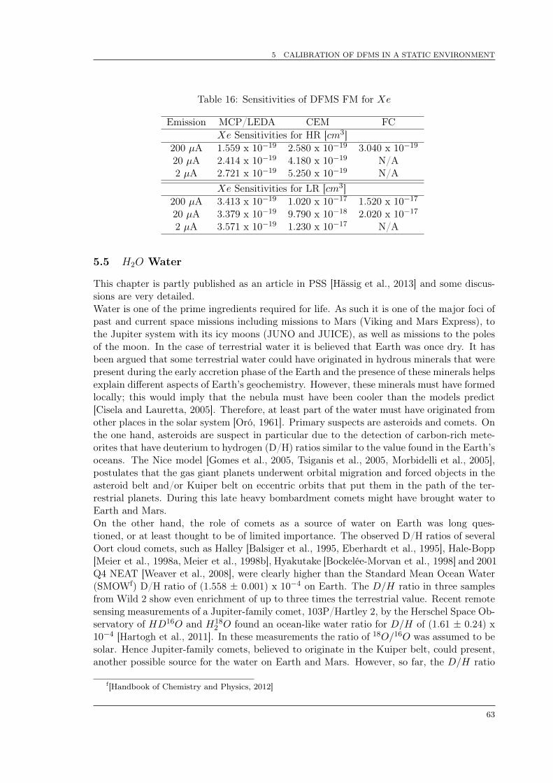
5 CALIBRATION OF DFMS IN A STATIC ENVIRONMENT
Table 16: Sensitivities of DFMS FM for Xe
Emission MCP/LEDA CEM FCXe Sensitivities for HR [cm3]
200 µA 1.559 x 10�19 2.580 x 10�19 3.040 x 10�19
20 µA 2.414 x 10�19 4.180 x 10�19 N/A2 µA 2.721 x 10�19 5.250 x 10�19 N/A
Xe Sensitivities for LR [cm3]200 µA 3.413 x 10�19 1.020 x 10�17 1.520 x 10�17
20 µA 3.379 x 10�19 9.790 x 10�18 2.020 x 10�17
2 µA 3.571 x 10�19 1.230 x 10�17 N/A
5.5 H2O Water
This chapter is partly published as an article in PSS [Hässig et al., 2013] and some discus-sions are very detailed.Water is one of the prime ingredients required for life. As such it is one of the major foci ofpast and current space missions including missions to Mars (Viking and Mars Express), tothe Jupiter system with its icy moons (JUNO and JUICE), as well as missions to the polesof the moon. In the case of terrestrial water it is believed that Earth was once dry. It hasbeen argued that some terrestrial water could have originated in hydrous minerals that werepresent during the early accretion phase of the Earth and the presence of these minerals helpsexplain different aspects of Earth’s geochemistry. However, these minerals must have formedlocally; this would imply that the nebula must have been cooler than the models predict[Cisela and Lauretta, 2005]. Therefore, at least part of the water must have originated fromother places in the solar system [Oró, 1961]. Primary suspects are asteroids and comets. Onthe one hand, asteroids are suspect in particular due to the detection of carbon-rich mete-orites that have deuterium to hydrogen (D/H) ratios similar to the value found in the Earth’soceans. The Nice model [Gomes et al., 2005, Tsiganis et al., 2005, Morbidelli et al., 2005],postulates that the gas giant planets underwent orbital migration and forced objects in theasteroid belt and/or Kuiper belt on eccentric orbits that put them in the path of the ter-restrial planets. During this late heavy bombardment comets might have brought water toEarth and Mars.On the other hand, the role of comets as a source of water on Earth was long ques-tioned, or at least thought to be of limited importance. The observed D/H ratios of severalOort cloud comets, such as Halley [Balsiger et al., 1995, Eberhardt et al., 1995], Hale-Bopp[Meier et al., 1998a, Meier et al., 1998b], Hyakutake [Bockelée-Morvan et al., 1998] and 2001Q4 NEAT [Weaver et al., 2008], were clearly higher than the Standard Mean Ocean Water(SMOWf) D/H ratio of (1.558 ± 0.001) x 10�4 on Earth. The D/H ratio in three samplesfrom Wild 2 show even enrichment of up to three times the terrestrial value. Recent remotesensing measurements of a Jupiter-family comet, 103P/Hartley 2, by the Herschel Space Ob-servatory of HD16O and H18
2 O found an ocean-like water ratio for D/H of (1.61 ± 0.24) x10�4 [Hartogh et al., 2011]. In these measurements the ratio of 18O/16O was assumed to besolar. Hence Jupiter-family comets, believed to originate in the Kuiper belt, could present,another possible source for the water on Earth and Mars. However, so far, the D/H ratio
f[Handbook of Chemistry and Physics, 2012]
63

5 CALIBRATION OF DFMS IN A STATIC ENVIRONMENT
for water could not be measured directly without at least the assumption of the 18O/16Oratio. This is the only D/H measurement in a Jupiter family comet. Nothing is knownabout the diversity among this group of comets. In addition, only four Oort cloud cometsare fairly small sample. Comet 67P/Churyumov-Gerasimenko, the target of the EuropeanSpace Agency’s Rosetta mission, most probably also originates from the Kuiper belt region.Rosetta will accompany the comet over an extended period of time. The rendezvous with thecomet will take place well beyond 3 AU and from then on Rosetta will perform observationsalong its inward journey to characterize the physical, chemical, and morphological character-istics of the nucleus and the surrounding coma including neutral gas, dust, and plasma. Incomparison to the to date only in situ measurements in a comet coma, the result of DFMSshould be clearly superior: The ion mass spectrometers on the Giotto spacecraft had limitedresolution and the D/H ratio was determined from the hydronium ion and not from thewater molecules directly [Balsiger et al., 1995, Eberhardt et al., 1995]. No attempts weremade so far to determine the oxygen isotopes in water in comets apart from the very coarsedetermination by the Ion Mass Spectrometer - High Intensity Sensor (IMS-HIS) on Giotto[Balsiger et al., 1995] which resulted in a solar value for 18O/16O with a large uncertainty.Therefore the observations by ROSINA at comet 67P/Churyumov-Gerasimenko are an im-portant step in confirming (or dismissing) the role of Kuiper belt objects as a major sourceof the water on Earth.The calibration measurements for H2O were performed for all detectors and all emissions atone pressure level. The pressure corrected for water was ⇠ 1 x 10�7 mbar while backgroundpressure was 5 x 10�10 mbar. CASYMIR was heated during the measurements to avoida water contamination of the chamber. Therefore the exact pressure measurements of thebackground might be underestimated. To put water into the chamber a gas bottle containingan amount of distilled water (1/10 of the volume) was pumped and the resulting water vaporintroduced into the chamber. The bottle contained an amount of air that was removed bypumping the bottle efficiently before mounting. However since the pressure inside the bottlewas lower than air pressure, some air could have leaked into the bottle during measurements,although during pumping no leak could be detected.The fragmentation measurements of H2O for the MCP/LEDA and the CEM can be found inFig. 41. The fragmentation measurements were not performed for the FC since it is expectedthat the detection efficiency for different species of the FC is comparable to that of the CEM.For comparison the values from NISTg and two other sources (Rao et al. (1995) and Orientand Srivastava (1987)) are given. The fragmentation pattern measured with DFMS FM isalmost comparable with the values given in NIST (and Rao et al. (1995)). However, theelectron energy of DFMS is reduced and therefore more signal due to the parent is expected.In Rao et al. (1995) the ionization cross section for 45 eV for H2O+, OH+, and O+ is givenwhile the fragmentation pattern is calculated relative to the H2O+. This fragmentation isalmost comparable to the fragmentation measured with DFMS FM. In Orient (1987) theionization cross section for 40 eV and 50 eV for H2O+, OH+, and O+ is given, thereforethe values were first interpolated and then the fragmentation pattern calculated relativeto the H2O+. This fragmentation pattern is clearly not in agreement with the measuredfragmentation of DFMS FM. Lots of different values can be found in the literature as thetwo examples show, although non of them really represents the measurements with DFMS
gIf NIST is referenced, data is from http : //webbook.nist.gov/chemistry/ from Mass spectrum. Alltough different values were found during several accessed from 05.02.2012-01.06.2013, the values are givenas a reference to state clearly, that the fragmentation pattern must be calibrated for every compound forDFMS.
64

5 CALIBRATION OF DFMS IN A STATIC ENVIRONMENT
Figure 41: The fragmentation pattern for H2O measured with DFMS FM for MCP/LEDAand CEM. For comparison NIST4, Rao 1995 and Orient 1987 is given. Although for thelatter two the electron energy of 45 eV was taken into account, they are not in agreementwith the measurements of DFMS FM. Uncertainties of the measurements are due to averagefor all emissions.
FM. Therefore the instrument characteristic fragmentation pattern has to be measured.The isotopic abundances measured for H2O are discussed one by one, and a summary canbe found in Tab. 17:
Table 17: Isotopic ratio and abundances of D/H and the oxygen isotope measured withMCP/LEDA.
Isotopic ratio Molecules Results Literature⇤
D/H HD16O/H162 O (1.68 ± 0.15) x 10�4 1.56 x 10�4
D/H HD18O/H182 O (1.47 ± 0.12) x 10�4 1.56 x 10�4
17O/16O H172 O/H16
2 O (4.00 ± 0.36) x 10�4 3.81 x 10�4
18O/16O 18OH/16OH (2.02 ± 0.12) x 10�3 2.05 x 10�3
18O/16O H182 O/H16
2 O (2.09 ± 0.19) x 10�3 2.05 x 10�3
16OD/17OH HD16O/H172 O 0.416 ± 0.029 0.409
⇤[Handbook of Chemistry and Physics, 2012]
There are two ways to measure the D/H ratio for water: One is to derive the ratio fromHD16O and H16
2 O. On the mass line 19 u/e there are HD16O, H172 O, and 18OH. The latter
two can be easily resolved in the high-resolution mode, while HD16O and H172 O still partly
overlap at the resolution of DFMS (see Fig. 42). Nevertheless, the two overlapping peakscan easily be resolved because of the well-defined shape and separate peak of 18OH on thesame spectra. The two overlapping peaks are clearly wider than the single peak. The peakof 18OH was fitted with a Gaussian shape and the full width half maximum (FWHM) from
65

5 CALIBRATION OF DFMS IN A STATIC ENVIRONMENT
this peak was taken for the fit of the two overlapping peaks. The only remaining parametersneeded to fit the two overlapping peaks are the corresponding amplitudes.
Figure 42: MCP/LEDA HR spectrum of mass 19 u/e, whereas H18O is clearly separatedfrom H17
2 O and HD16O. The Full Width at Half Maximum (FWHM) of the peak to theright is significantly broader than that for H18O and implies two overlapping peaks. Toresolve the latter, two Gaussian fits were applied; taking the FWHM from H18O as fixedfor all three mass peaks and the amplitudes of H17
2 O and HD16O as the free parameters tobe fitted.
The other clever measurement is to deduce the D/H ratio from rarer isotopes such as H182 O
and HD18O. On the 21 u/e mass line there is no signal from any other molecule exceptHD18O with a very minor contribution of D17
2 O (< 10�4 relative to HD18O [Handbookof Chemistry and Physics, 2012]). So there is no need for the high-resolution mode toresolve individual species and the measurement can be performed in the more sensitive low-resolution mode. Note that in low-resolution mode, H18
2 O on the 20 u/e mass line competeswith FH (fluorine and FH are part of the background, mostly due to vacuum grease, e.g.Braycote [Schläppi et al., 2010]). The ratio H18
2 O/H19F however, can be derived from thehigh-resolution mode, where H19F can easily be separated from H18
2 O.The isotopic ratio deduced from mass line 18 u/e and 19 u/e are measured in high resolutionand therefore not on the same spectrum, which results in a calibration error due to differentDFMS MCP/LEDA detector gain (5%). Other uncertainties are due to statistical errorsand the mathematical fit (7%) to resolve HD16O from H17
2 O (see Fig. 42). This resultsin a total uncertainty of ⇠ 9%. For the ratio of H18
2 O/HD18O the measurements wereperformed in low resolution, taking advantage of higher sensitivity of the instrument as wellas the advantage of having both peaks on the same spectrum to avoid calibration errors fromthe detector gain. Because of the limited dynamic range for one single spectrum, the peakof the more abundant isotope is in saturation and has to be fitted. The total uncertaintyof ⇠ 8% contains the uncertainty of the fit and the statistical uncertainties (7%) of the HR
66

5 CALIBRATION OF DFMS IN A STATIC ENVIRONMENT
spectrum required to deduce the ratio of H182 O to FH on the mass 20 u/e.
The uncertainties of H172 O/H16
2 O (see Fig. 42) have the same causes as the measurementsof HD16O/H16
2 O and therefore a total of ⇠ 9%.The only measurement of the relative abundance of oxygen isotopes in the coma of a cometis the ratio of 18O/16O measured at Halley. As is the case for the D/H ratio the only in situmeasurements are from the Giotto flyby where a telluric ratio was found with IMS-HIS to be(1.93 ± 0.12) x 10�3 [Balsiger et al., 1995] and the Neutral Mass Spectrometer to be (2.13 ±0.18) x 10�3 [Eberhardt et al., 1995]. Remote sensing measurements of the Halley coma arein line with these in situ measurements and are within error bars compatible with the ratioon Earth. The in situ measurements with DFMS at comet 67P/Churyumov-Gerasimenkowill not only provide the 18O/16O ratio but furthermore enable a unique opportunity todirectly measure the 17O/16O ratio. The 17O/16O ratio can be derived from mass 19 u/e inthe same way as the D/H ratio with a well defined mathematical fit. The oxygen isotopicratio 18O/16O can be measured twice; once for H18
2 O/H162 O and once for H18O/H16O. For
the second ratio, the individual instrumental fragmentation pattern of water has to be wellcalibrated to adapt the ratio of hydroxyl to water.Hydroxyl is clearly separated from Ammonia in HR. The same is true for 18OH from HD16Oand H17
2 O; therefore the remaining uncertainties are due to gain calibration (5%) and sta-tistical errors (1%). This results in a total uncertainty of ⇠ 6%. H18
2 O and FH on massline 20 u/e partly overlap at the base of the line but are clearly separated at the peak. Toresolve the two peaks, a mathematical fit was applied. The total error of ⇠ 9% is due todetector gain (5%), statistics and mathematical fit (7%), whereas on mass line 18 u/e thecontribution of 18O, 17OH, and 16OD can be neglected since their abundance is in the orderof < 10�4 compared to H18
2 O [Handbook of Chemistry and Physics, 2012].The sensitivity measurements were performed for all detectors and emissions. The totalsignal for the sensitivity contains the signal of H2O, the signal of all fragments (O, OH)and the signal of all isotopes. The sensitivity for the MCP/LEDA and CEM for 200 µA islower than for the other emissions. The sensitivity for the FC is in good agreement withthat of the CEM, however no signal could be detected for the FC for 20 µA and 2 µA. Thefactor between 200 µA and 2 µA is much lower than for other compounds. A possible reasonfor this could be that the background pressure was underestimated for this measurementsince CASYMIR was heated during these measurements and therefore more backgroundmaterial could be released from the walls. An other explanation could be that the bottle,although pumped efficiently before the measurement contained still some air. Therefore thesensitivity of the measurements of 200 µA might be underestimated and evaluation of thedata using this number should be analyzed carefully.The statistical error for the sensitivity measurement is < 1%. The uncertainties of the pres-sure measurement are ⇠14% (see App. F). Calibration uncertainties of the MCP/LEDAsuch as gain calibration and individual pixel gain corrections are estimated as ⇠ 7%. Cali-bration uncertainties of the CEM and the FC detector are assumed to be ⇠ 5%. The totaluncertainties for the sensitivity in HR are therefore: 16% for MCP/LEDA and 15% forCEM & FC. The evaluation of the proportion of the signal in LR is deduced from the HRspectra therefore an additional uncertainty (⇠ 5%) has to be taken into account, leading toslightly higher uncertainties. Uncertainties for the sensitivity in LR are therefore: 17% forMCP/LEDA and 16% for CEM & FC.The measurement of D/H can be done within one single spectrum and therefore an integra-tion time of only 20 s is needed at a water vapor pressure of 3.0 x 10�7 mbar. For comparison:at the comet at 3 AU, and to reduce statistical errors below the 5% level measuring the iso-
67

5 CALIBRATION OF DFMS IN A STATIC ENVIRONMENT
Table 18: Sensitivities of DFMS FM for H2O
Emission MCP/LEDA CEM FCH2O Sensitivities for HR [cm3]
200 µA 2.308 x 10�19 1.337 x 10�19 1.282 x 10�19
20 µA 1.396 x 10�18 8.944 x 10�19 N/A2 µA 1.151 x 10�18 1.138 x 10�18 N/A
H2O Sensitivities for LR [cm3]200 µA 5.092 x 10�18 3.295 x 10�18 4.636 x 10�18
20 µA 1.823 x 10�17 1.327 x 10�17 N/A2 µA 1.402 x 10�17 1.069 x 10�17 N/A
topic ratio requires the accumulation of 256 spectra with an ion source emission current of200 µA, or a total integration time of 5120 s, assuming a modeled water number density at 3AU of 4 x 106 cm�3 at 20 km above the surface of 67P/Churyumov-Gerasimenko. The den-sity is derived with an interpolated molecule flux of 1025 molecules/s [Tenishev et al., 2008].With the assumption of a spherically outgassing comet and at a temperature of 180 K thatresults in a mean velocity of 460 m/s for water molecules.
5.6 N2 Nitrogen
The abundance of N2 in the coma of comets is an ongoing process, since the signal ofN2 and CO can be found on the same mass (28 u/e) for mass spectrometers. Howeveran upper limit for N2/H2O of 0.1 was found for comet Halley [Eberhardt et al., 1988].Isotopic ratios for 14N/15N are not deduced directly for N2 but in comet Hale-Bopp forCN [Arpigny et al., 2003] and HCN [Ziurys et al., 1999], while the later measurement iscompatible with the terrestrial value of 273 [Handbook of Chemistry and Physics, 2012].The first measurement indicates an unidentified additional source of CN since the iso-topic ratio of 14N/15N is 140 ± 35 and not compatible with the terrestrial value. Areevaluation of the ratios found that value for CN and HCN are both not compati-ble with the terrestrial value [Bockelée-Morvan et al., 2008]. In addition the ratios mea-sured for Jupiter family comet 17P/Holmes is not compatible with the terrestrial value[Bockelée-Morvan et al., 2008]. These results indicate that HCN is the parent of CN incometary atmospheres. The higher abundance of 15N compared to Earth atmosphere in-dicates an isotopic fractionation of the N volatiles in the solar nebula during formation ofthe solar system [Bockelée-Morvan et al., 2008]. This indicates that there was no isotropi-cally equilibration between the main nitrogen reservoir in the solar system and the HCNmolecules before they were incorporated in Oort Cloud and Kuiper Belt comets.The calibration measurements for N2 were performed for all detectors and all emissionsat one pressure level (1 x 10�7 mbar with a background pressure of 4 x 10�10 mbar).A correction factor for the pressure was not applied since the pressure measurements arecalibrated for N2. The calibration measurements are performed manually to reduce pixelgain correction.The isotopic abundances for 15N/14N for 15N14N/14N2 measured with the MCP/LEDAdetector for all emissions can be found in Fig. 43. The measurements for HR and LR arewithin uncertainties comparable with the literature value. Error bars are due to statisticaluncertainties (< 2%) and calibration uncertainties of the MCP/LEDA (5%). An other
68

5 CALIBRATION OF DFMS IN A STATIC ENVIRONMENT
Figure 43: Comparison of the DFMS measurements for 15N/14N with literature value forthe MCP/LEDA. 15N/14N ratio is measured for 15N14N relative 14N2.
possibility is to deduce the isotopic abundance on the fragment 14N of 14N2 and the isotope15N . On mass 15 u/e the peaks of 15N , 14NH, 12CH3 are well separated in HR thesame is true for 14N and CH2. This was tested for the MCP/LEDA for an emission of200 µA in HR and the ion current of 15N was 0.34% of 14N within uncertainties due tostatistics of 2% and calibration of 5% the measurement is in agreement with literature(0.369% [Handbook of Chemistry and Physics, 2012]).
Table 19: Sensitivities of DFMS FM for N2
Emission MCP/LEDA CEM FCN2 Sensitivities for HR [cm3]
200 µA 1.989 x 10�19 2.193 x 10�19 1.783 x 10�19
20 µA 6.797 x 10�19 8.486 x 10�19 6.900 x 10�19
2 µA 8.643 x 10�19 1.713 x 10�18 1.393 x 10�18
N2 Sensitivities for LR [cm3]200 µA 5.061 x 10�18 5.682 x 10�18 6.240 x 10�18
20 µA 1.018 x 10�17 1.172 x 10�17 1.287 x 10�17
2 µA 1.046 x 10�17 1.740 x 10�17 1.911 x 10�17
Sensitivity measurements were performed in LR and HR for all detectors and emissions forone pressure level (see Tab. 19). The total signal includes isotopic abundances (14N/14N :100%, 15N/14N :0.37%) and the signal on 14 u/e for the fragment and the doubly charged N2
of ⇠5%. The sensitivity for an emission of 200 µA is lower than the other emissions for alldetectors. The sensitivity for the FC is slightly lower than for the CEM. The statistical errorfor the sensitivity measurement is < 1%. The uncertainties of the pressure measurement are⇠14% (see App. F). Calibration uncertainties of the MCP/LEDA such as gain calibration
69

5 CALIBRATION OF DFMS IN A STATIC ENVIRONMENT
Figure 44: Fragmentation pattern for CO2 for the MCP/LEDA and the CEM compared toNIST.
and individual pixel gain corrections are estimated as ⇠ 7%. Calibration uncertaintiesof the CEM and the FC detector are assumed to be ⇠ 5%. The total uncertainties forthe sensitivity in HR are therefore: 16% for MCP/LEDA and 15% for CEM & FC. Theevaluation of the proportion of the signal in LR is deduced from the HR spectra thereforean additional uncertainty (⇠ 5%) has to be taken into account, leading to slightly higheruncertainties. Uncertainties for the sensitivity in LR are therefore: 17% for MCP/LEDAand 16% for CEM & FC.
5.7 CO2 Carbon dioxide
The presence of CO2 in cometary coma was indirectly established long time ago from theexistence of CO+
2 ions in the cometary tail [Feldman et al., 2004]. The production rate ofCO2 relative to H2O for comet Hale-Bopp was more than 20%, however there exist onlyobservations for r > 2.9 AU for this comet. The production rate for CO2 for 1P/Halleywas 3–4% and for 103P/Hartley was 8–10% [Bockelée-Morvan et al., 2004]. The higherproduction rate of Hale-Bopp can be explained by the higher volatility of CO2 comparedto H2O at that distance from the Sun. The isotopic ratios in comets for C and O are notdeduced from CO2 nor fragments thereof.The calibration measurements for CO2 were performed for all detectors and all emissions atone pressure level. The background pressure was 8 x 10�10 mbar and the pressure correctedfor CO2 while gas was introduced was 7 x 10�8 mbar. The calibration measurements wereperformed with measurement modes for the MCP/LEDA and CEM detector while for theFC the measurements were performed manually. There exist special calibration modes forCO2, however since this modes do not measure isotopic ratios of the fragments (17 u/e, 18u/e and 29 u/e), scan modes for LR and HR were used.The fragmentation pattern for CO2 for the MCP/LEDA and the CEM compared to NISTcan be found in Fig. 44. Uncertainties are due to average values for all emissions. The
70

5 CALIBRATION OF DFMS IN A STATIC ENVIRONMENT
fragmentation pattern for the CEM is higher for the parent than the NIST, and there-fore less for the fragments. This can be explained by the lower electron energy in the ionsource. The fragmentation pattern of the MCP/LEDA is not the same as for the CEM.This can be explained by the detection efficiency of the MCP. However since the mass rangeof the MCP/LEDA does not cover 12 u/e the fragment C is not taken into account for theMCP/LEDA.
Figure 45: The measured isotopic ratios of CO2 with the MCP/LEDA for an emission of200 µA relative to literature value.
The isotopic abundances of CO2 measured with the MCP/LEDA with an emission of 200 µAcan be found in Fig. 45. All isotopic abundances are within uncertainties in good agreementwith the literature value. Uncertainties are due to statistical errors and calibration errorsof the detector of 5%. Uncertainties are dominated by the calibration errors except themeasurements for 17O/16O with statistical uncertainties of 5% and 13C17O16O/12C16O2
with statistical uncertainties of 9%. The isotopic ratios for 17O and 18O could only beisolated from the more dominant peaks on the same mass (16OH on 17 u/e and H16
2 O on18 u/e), because the background pressure and therefore the water signal was very low. Toobtain this ratios at the comet might be difficult since the water signal is very prominent.However to distinguish a low signal like expected for 18O from a much higher signal likeH16
2 O, a peak fit with respect to the slightly broader foot of the peak has to be used.Therefore a combination of a Gauss and Lorentz peak shape was used (Pseudo-Voigt). Theuncertainties of the fit compared to the raw data is smaller than the statistical uncertaintiesof the peak itself.The sensitivity measurements were performed for all detectors and all emissions. The totalsignal for CO2 for the MCP/LEDA includes the signal of the parent, the fragments, allmeasured isotopic abundances for the parent and the fragments, and the amount of doublycharged parents (0.01%). The statistical error for the sensitivity measurement is < 1%.The uncertainties of the pressure measurement are ⇠14% (see App. F). Calibration uncer-tainties of the MCP/LEDA such as gain calibration and individual pixel gain correctionsare estimated as ⇠ 7%. Calibration uncertainties of the CEM and the FC detector are
71

5 CALIBRATION OF DFMS IN A STATIC ENVIRONMENT
Table 20: Sensitivities of DFMS FM for CO2
Emission MCP/LEDA CEM FCCO2 Sensitivities for HR [cm3]
200 µA 1.538 x 10�19 4.540 x 10�19 4.727 x 10�19
20 µA 5.835 x 10�19 1.373 x 10�19 2.895 x 10�18
2 µA 6.601 x 10�19 1.403 x 10�19 2.865 x 10�18
CO2 Sensitivities for LR [cm3]200 µA 2.107 x 10�18 5.610 x 10�18 1.765 x 10�17
20 µA 6.001 x 10�18 9.223 x 10�19 1.805 x 10�17
2 µA 7.034 x 10�18 1.005 x 10�18 3.151 x 10�17
assumed to be ⇠ 5%. The total uncertainties for the sensitivity in HR are therefore: 16%for MCP/LEDA and 15% for CEM & FC. The evaluation of the proportion of the signal inLR is deduced from the HR spectra therefore an additional uncertainty (⇠ 5%) has to betaken into account, leading to slightly higher uncertainties. Uncertainties for the sensitivityin LR are therefore: 17% for MCP/LEDA and 16% for CEM & FC.
72

5 CALIBRATION OF DFMS IN A STATIC ENVIRONMENT
5.8 Alkanes
Alkanes are acyclic branched or un-branched hydrocarbons having the general formulaCnH2n+2, and therefore consisting entirely of hydrogen atoms and saturated carbon atoms[Moss et al., 1995]. The detection of alkanes in comets are confirmed for CH4 and C2H6,while for C3H8 the search has been negative so far [Bockelée-Morvan et al., 2004]. The fol-lowing information is a summary of [Bockelée-Morvan et al., 2004]: CH4 and C2H6 werefirst clearly spectroscopically detected in comet Hyakutake, through ground based obser-vations in 1996. In every comet searched since then, Methane and Ethane was detected.The abundance of CH4/H2O varies from 0.14% to 1.4%. Among Oort cloud comets, theabundance for C2H6/H2O is remarkably constant (⇠ 0.6%), with the exception of C/1999S4 (LINEAR). In comet Halley an abundance of 0.4% was found with in situ measurementsof NMS.
5.8.1 CH4 Methane
Methane can be found in the background of Rosetta due to spacecraft outgassing, thereforea careful subtraction of the background is necessary for an absolute density in the cometscoma relative to water.Calibration measurements for CH4 for all detectors and emissions were performed at onepressure level (1 x 10�7 mbar, background pressure 1 x 10�9 mbar). The pressure measure-ments are relative to N2 since no correction factor is given for CH4. A possible correctionfactor of 0.56 – 0.71 is found for a similar pressure sensor [Controller, 2001], however sincethis factor is not given for the used pressure sensor a correction was not applied.
Figure 46: The fragmentation pattern for CH4 for MCP/LEDA and CEM compared toNIST. Errorbars for MCP/LEDA and CEM are due to the average for all emissions.
The fragmentation pattern for CH4 for MCP/LEDA and CEM relative to NIST can be foundin Fig. 46. The fragmentation patterns shows more parents than fragments compared toNIST. This can be explained by the lower electron energy in the ion source compared to
73

5 CALIBRATION OF DFMS IN A STATIC ENVIRONMENT
NIST. The differences between MCP/LEDA and CEM can be explained by the detectionefficiency of the MCP.
Figure 47: Isotopic abundances measured with DFMS relative to literature values for CH4.
Isotopic abundances for 13C/12C for the CEM and 13CH4/12CH4 for the MCP/LEDA forall emissions can be found in Fig. 47. All measurements are in agreement with the liter-ature value, however for the CEM measurements the statistical uncertainties dominate theuncertainties due to calibration errors. Statistical uncertainties for the CEM measurementsare: 200 µA 13%, 20 µA 26%, and 2 µA 60%. Statistical uncertainties for the MCP/LEDAmeasurements are: 200 µA 0.4%, 20 µA 0.7%, and 2 µA 1%. The total uncertainty containsalso calibration uncertainties of 7% for the MCP/LEDA and 5% for the CEM. The statisti-cal uncertainties for the CEM could be reduced by a longer integration time or the sum ofseveral spectra.
Table 21: Sensitivities of DFMS FM for CH4
Emission MCP/LEDA CEM FCCH4 Sensitivities for HR [cm3]
200 µA 5.661 x 10�19 9.990 x 10�19 9.440 x 10�19
20 µA 6.059 x 10�19 1.339 x 10�18 1.700 x 10�18
2 µA 3.247 x 10�19 1.829 x 10�18 N/ACH4 Sensitivities for LR [cm3]
200 µA 1.153 x 10�17 1.306 x 10�17 9.480 x 10�18
20 µA 1.920 x 10�17 2.354 x 10�17 2.650 x 10�17
2 µA 2.389 x 10�17 2.816 x 10�17 1.430 x 10�17
Sensitivity measurements for all detectors and emissions for LR and HR can be found inTab. 21. The density for CH4 is given relative to N2, since the pressure measurementswere not corrected. Therefore sensitivities for CH4 are given relative to N2. The total
74

5 CALIBRATION OF DFMS IN A STATIC ENVIRONMENT
signal for CH4 contains the signal of the parent, all fragments, and isotopic abundances for13C/12C and 13CH4/12CH4. No doubly charged parent could be detected since the massrange for DFMS does not cover 8 u/e. The sensitivity for the FC is in good agreementwith the CEM sensitivities, however no signal could be detected for 2 µA for the FC inHR. The sensitivities for 200 µA are slightly lower then for the other emissions, with theexception of the MCP/LEDA in HR, where the sensitivity for 2 µA is lower than for 200µA. A possible reason for this could be that the instrument had to be switched of severaltimes during the measurements of the MCP/LEDA for 2 µA due to software problems.Therefore the background measurements for the MCP/LEDA were performed with a ’cold’instrument and might be underestimated. The factor between the sensitivity for LR andHR is due to the resolution sensitive slit, which explains a factor of ⇠ 14, further differencesare due to ion optical differences for LR and HR. The statistical error for the sensitivitymeasurement is < 1%. The uncertainties of the pressure measurement are ⇠14% (see App.F). Calibration uncertainties of the MCP/LEDA such as gain calibration and individualpixel gain corrections are estimated as ⇠ 7%. Calibration uncertainties of the CEM and theFC detector are assumed to be ⇠ 5%. The total uncertainties for the sensitivity in HR aretherefore: 16% for MCP/LEDA and 15% for CEM & FC. The evaluation of the proportionof the signal in LR is deduced from the HR spectra therefore an additional uncertainty (⇠5%) has to be taken into account, leading to slightly higher uncertainties. Uncertainties forthe sensitivity in LR are therefore: 17% for MCP/LEDA and 16% for CEM & FC.
75

5 CALIBRATION OF DFMS IN A STATIC ENVIRONMENT
5.8.2 C2H6 Ethane
Ethane can be found in the background of Rosetta due to spacecraft outgassing [Schläppi et al., 2010],therefore a careful subtraction of the background is necessary for an absolute density in thecomets coma relative to water.The calibration measurements for C2H6 were performed for all detectors and emissions at onepressure level. The pressure during measurements was 1 x 10�7 mbar and the backgroundpressure before introducing gas into the chamber was 5 x 10�10 mbar. The pressure mea-surements are relative to N2 since no pressure correction factor is given for C2H6. A possiblecorrection factor of 0.357 – 0.400 is found for a similar pressure sensor [Controller, 2001],however since this factor is not given for the used pressure sensor a correction was not ap-plied. The measurements were performed with measurement modes for the MCP/LEDAand CEM, and manually for 30 u/e for the FC.
Figure 48: The fragmentation pattern of C2H6 measured with the MCP/LEDA and theCEM. For comparison NIST values are given. Error bars are due to standard deviation ofthe average for all emissions.
The fragmentation pattern of C2H6 for the MCP/LEDA and the CEM can be found in Fig.48. The fragmentation pattern for both detectors are deduced from the measurements ofall emissions. The average values for all emissions are given in Fig. 48. Uncertainties ofthe fragmentation pattern are due to standard deviation of the average of all emission forone detector. Statistical uncertainties are in the same range or lower than the standarddeviation. The fragmentation behavior of the ion source DFMS FM is almost in agreementwith the NIST values although the electron energy is lower. The ratio of the parent isslightly higher for DFMS FM than the ratio in NIST while for other fragments the valuesare comparable. Differences between the MCP/LEDA and the CEM can be explained bythe different detection efficiencies of the detectors.The isotopic measurements presented here are 13C12CH6/12C2H6 measured with the MCP/LEDA
76

5 CALIBRATION OF DFMS IN A STATIC ENVIRONMENT
Figure 49: Isotopic measurements of C2H6 with the MCP/LEDA (black) and the CEM(red). The measurements are in good agreement with literature value, however the statisticaluncertainties for the 13C/ 12C measured with the CEM are rather high. Mass 12 can onlybe measured with the CEM, therefore no measurements for the MCP/LEDA are availablefor 13C/ 12C
and the CEM for all emission and 13C/12C measured with the CEM (see Fig. 49). Theisotopic measurements are in good agreement with the literature value, however the statis-tical uncertainties for the CEM measurements are rather high since the amount of C dueto fragmentation is very low (< 1%). For an emission of 200 µA the statistical uncertaintyis 46% and for the other emissions they are 140% for 2 µA and 100% for 20 µA. Howeverthe measurement itself is in remarkably good agreement with literature. Uncertainties ofthe isotopic measurements with the MCP/LEDA of 13C12CH6/12C2H6 are dominated bythe calibration uncertainty of 7% for all emissions. The statistical uncertainties are < 1%for all emissions. The isotopic measurement with the CEM are also in good agreement withliterature. The statistical uncertainties for the isotopic measurements of the CEM are 3%,4%, and 10% for 200 µA, 20 µA, and 2 µA.
Table 22: Sensitivities of DFMS FM for C2H6
Emission MCP/LEDA CEM FCC2H6 Sensitivities for HR [cm3]
200 µA 8.712 x 10�20 1.627 x 10�19 1.192 x 10�19
20 µA 3.108 x 10�19 6.281 x 10�19 6.298 x 10�19
2 µA 4.596 x 10�19 1.064 x 10�18 N/AC2H6 Sensitivities for LR [cm3]
200 µA 2.715 x 10�18 4.983 x 10�18 5.434 x 10�18
20 µA 4.898 x 10�18 8.598 x 10�18 9.097 x 10�18
2 µA 8.980 x 10�18 9.730 x 10�18 8.949 x 10�18
77

5 CALIBRATION OF DFMS IN A STATIC ENVIRONMENT
The sensitivity measurement for all detectors and emissions can be found in Tab. 22. Nosignal was detected for 2 µA with the FC, therefore the sensitivity is marked with N/A.The total signal for sensitivity calculations of C2H6 contains the signal of the parent, thefragments and the signal of the isotopes 13C12CH6 for all detectors and 13C for the CEM.The sensitivities are relative to N2 since the pressure was not corrected for C2H6. Thesensitivities for 200 µA are clearly lower than for the other emissions. An explanationtherefore could be that the space charge because of the higher density of electrons for 200 µAemission around the filament, harms the entrance of the electrons into the ionization region.The electrons have to pass a slit before entering the ionization region, and less electrons areentering the ion source through that slit because they diverge due to space charge. The factorbetween sensitivities of the MCP/LEDA and the CEM in HR are rather high comparedto LR. The statistical error for the sensitivity measurement is < 1%. The uncertaintiesof the pressure measurement are ⇠14% (see App. F). Calibration uncertainties of theMCP/LEDA such as gain calibration and individual pixel gain corrections are estimated as⇠ 7%. Calibration uncertainties of the CEM and the FC detector are assumed to be ⇠ 5%.The total uncertainties for the sensitivity in HR are therefore: 16% for MCP/LEDA and15% for CEM & FC. The evaluation of the proportion of the signal in LR is deduced fromthe HR spectra therefore an additional uncertainty (⇠ 5%) has to be taken into account,leading to slightly higher uncertainties. Uncertainties for the sensitivity in LR are therefore:17% for MCP/LEDA and 16% for CEM & FC.
78

5 CALIBRATION OF DFMS IN A STATIC ENVIRONMENT
5.8.3 C3H8 Propane
A small amount of Propane can be found in the background of Rosetta due to spacecraft out-gassing [Schläppi et al., 2010], therefore a careful subtraction of the background is necessaryfor an absolute density in the comets coma relative to water. Furthermore the knowledgeabout the fragmentation pattern might help to identify fragments of the parent molecule.
Figure 50: Fragmentation pattern for C3H8 measured with MCP/LEDA and CEM, withthe average for all emissions compared to NIST. Error bars are due to standard deviationof the average.
Calibration measurements for C3H8 for all detectors and emissions were performed at onepressure level (1 x 10�7 mbar, background pressure 1 x 10�9 mbar). The pressure measure-ments are relative to N2 since no correction factor is given for C3H8. A possible correctionfactor of 0.24 – 0.28 is found for a similar pressure sensor [Controller, 2001], however sincethis factor is not given for the used pressure sensor a correction was not applied.The fragmentation pattern for MCP/LEDA and CEM compared to NIST can be found inFig. 50. Error bars of the MCP/LEDA and CEM are the standard deviation of the averageof all emission. In principle the amount of fragments relative to the parent molecule issmaller compared to NIST. However the fragment CH4 is definitely higher than in NIST.First a contamination from the measurement before was suggested, but later measurementshow the same ratio for CH4 relative to the parent molecule. An other contamination sourcecould be from Air, while leaking in between bottle and valve. This could also be ruled outbecause the signal for Ar, N2, O2, CO2 and H2O are within statistical uncertainties in thesame order as background measurements. In summary the fragmentation pattern values forthe lighter fragments (m CH4), should be used with care.Measurements of the isotopic abundances are possible for the fragments that are saturated(CH4 and C2H6) and the parent molecule itself as well as the 13C/12C ratio. Since otherpeaks of the isotopes overlap with the signal of the heavier fragment and are not necessarily
79

5 CALIBRATION OF DFMS IN A STATIC ENVIRONMENT
Figure 51: Isotopic abundances for C3H8 relative to literature value.
resolvable. The measured isotopic abundances for the MCP/LEDA for an emission of 200µA and the CEM can be found in Fig. 51. The isotopic abundance for 13C of the parentmolecule 12C3H8 and the fragment 12C2H6 measured with the MCP/LEDA are in goodagreement with the literature value within uncertainties. Uncertainties are due to statistics(< 1%) and calibration (5%). Further isotopic ratios for D/H and 13C for the MCP/LEDAare not in agreement with literature values. They are both higher than the literature value.A depletion for the isotopic abundances could be explained by the fragmentation pattern,since the fragmentation pattern shows a significant high signal compared to NIST for CH4.However the two peaks for 13CH4 and 12CDH3 are clearly separated and do not overlapwith 15NH2 or 14NH3. A signal due to doubly charged particles on this mass (17 u/e)is also not possible since no signal could be detected for 34 u/e. The isotopic abundancesfor 13C measured with the CEM are in good agreement with literature value, howeverstatistical uncertainties are rather high: 10% for 13CH4/12CH4, and 40% for 13C/12C.Since the integration time of the CEM is nominal 1 s per step while the integration timefor the MCP/LEDA is 19.8 s, the statistical uncertainties are higher for the CEM than theMCP/LEDA. An other reason for the rather high statistical uncertainties is that only 1%of the total signal for propane is found as fragment on 12C.Sensitivity measurements for all detectors and emissions for LR and HR can be found inTab. 23. The density C3H8 is relative to N2, since the pressure was not corrected, thereforesensitivities are relative to N2. The total signal for C3H8 contains the signal of all fragments,isotopic abundances as discussed for Fig. 51. No doubly charged parent molecule could bedetected for C3H8 on mass 22 u/e. This is expected since hydrocarbons do more likelyfragment, than get doubly charged. And because the electron energy energy is reduced,the amount of doubly charged particles is reduced as well. The sensitivity for the FC isin agreement with the CEM sensitivities for 200 µA in LR but slightly higher for HR. Nosignal could be detected for FC with 20 µA in HR and 2 µA for C3H8. The sensitivity for200 µA is lower than for the other emissions. The factor between the sensitivity for LR andHR is due to the resolution sensitive slit, which explains a factor of ⇠ 14, further differences
80

5 CALIBRATION OF DFMS IN A STATIC ENVIRONMENT
Table 23: Sensitivities of DFMS FM for C3H8
Emission MCP/LEDA CEM FCC3H8 Sensitivities for HR [cm3]
200 µA 8.196 x 10�20 3.248 x 10�19 5.089 x 10�19
20 µA 3.249 x 10�19 7.501 x 10�19 N/A2 µA 2.872 x 10�19 9.611 x 10�19 N/A
C3H8 Sensitivities for LR [cm3]200 µA 1.409 x 10�18 5.501 x 10�18 5.795 x 10�18
20 µA 3.793 x 10�18 9.145 x 10�18 1.050 x 10�17
2 µA 4.107 x 10�18 1.102 x 10�17 N/A
are due to ion optical differences for LR and HR.The statistical error for the sensitivity measurement is < 1%. The uncertainties of the pres-sure measurement are ⇠14% (see App. F). Calibration uncertainties of the MCP/LEDAsuch as gain calibration and individual pixel gain corrections are estimated as ⇠ 7%. Cali-bration uncertainties of the CEM and the FC detector are assumed to be ⇠ 5%. The totaluncertainties for the sensitivity in HR are therefore: 16% for MCP/LEDA and 15% forCEM & FC. The evaluation of the proportion of the signal in LR is deduced from the HRspectra therefore an additional uncertainty (⇠ 5%) has to be taken into account, leading toslightly higher uncertainties. Uncertainties for the sensitivity in LR are therefore: 17% forMCP/LEDA and 16% for CEM & FC.
81

5 CALIBRATION OF DFMS IN A STATIC ENVIRONMENT
5.8.4 C4H10 Butane
Butane can be found in the background measurements of the spacecraft, due to outgassing(see Schläppi et al. (2010)).The calibration measurements of Butane were performed with n-Butane and contain mea-surements of all detectors and emissions. The pressure during measurements was 1 x 10�7
mbar and the background pressure before introducing gas into the chamber was 5 x 10�10
mbar. The pressure measurements are relative to N2 since no pressure correction factor isgiven for C4H10. A possible correction factor of 0.204 – 0.213 is found for a similar pressuresensor [Controller, 2001], however since this factor is not given for the used pressure sensora correction was not applied. The measurements were performed with measurement modesfor the MCP/LEDA and CEM, and manually for 58 u/e for the FC.The fragmentation pattern for C4H10 measured with MCP/LEDA and CEM can be found inFig. 52. The values given are the average of the ratios for all emissions of one detector. Thestandard deviation is taken as uncertainties for the ratios. Uncertainties due to statisticsare smaller than standard deviation. The fragmentation pattern of DFMS contains moreheavier fragments compared to NIST, especially in the measurements with CEM the amountof C4H10 is higher. Differences between the MCP/LEDA and the CEM are given by thedetection efficiency of the MCP/LEDA. One can clearly see that the detection efficiency forthe MCP/LEDA for the heavier masses is lower than for the CEM.The isotopic measurements are limited to the heaviest fragments of the Alkanes (CnH2n+2, n= 1 ... 4) since the isotopes of the other fragments do overlap with heavier fragments at theresolution of the instrument. The measurements presented are in HR for an emission of 200µA for the CEM and the MCP/LEDA (see Fig. 53). All measurements are in good agreementwith literature values. The isotopic ratio of 13C/12C measured with the CEM has ratherhigh uncertainties due to statistics (80%). 13CH4/12CH4 could be measured with the CEMand the MCP/LEDA, statistical uncertainties for the MCP/LEDA are 3%, and 13% for theCEM. The total uncertainty contains also calibrations uncertainties of the MCP/LEDA (7%)and the CEM (5%). To resolve 13CH4 from 12CDH3 a Gauss fit was applied since the twopartly overlap at the resolution of the instrument with the MCP/LEDA. The uncertaintiesof the fit are smaller than the statistical error, therefore no additional error was taken intoaccount. The statistical uncertainties of 12CDH3/12CH4 are 12%. For the other ratiosthe statistical uncertainties are < 1% and the total uncertainties are dominated by thecalibration error.The sensitivity measurements for C4H10 for all detectors and emissions can be found in Tab.24. The sensitivities are relative to N2 since the pressure was not corrected for C4H10. Thesensitivity of the CEM is much higher compared with them of the MCP/LEDA. The mainreason therefore is that the detection efficiency of the MCP/LEDA is decreasing with mass.No signal could be detected for C4H10 with an emission of 2 µA for the FC and in HR foran emission of 20 µA. Since the measurements with the FC were only done on C4H10, asignal could have been detected for a more abundant fragment. However the sensitivity ofthe FC is in agreement with the CEM sensitivity and therefore the CEM sensitivity couldbe used as reference for the FC.The statistical error for the sensitivity measurement is < 1%. The uncertainties of the pres-sure measurement are ⇠14% (see App. F). Calibration uncertainties of the MCP/LEDAsuch as gain calibration and individual pixel gain corrections are estimated as ⇠ 7%. Cali-bration uncertainties of the CEM and the FC detector are assumed to be ⇠ 5%. The totaluncertainties for the sensitivity in HR are therefore: 16% for MCP/LEDA and 15% for
82
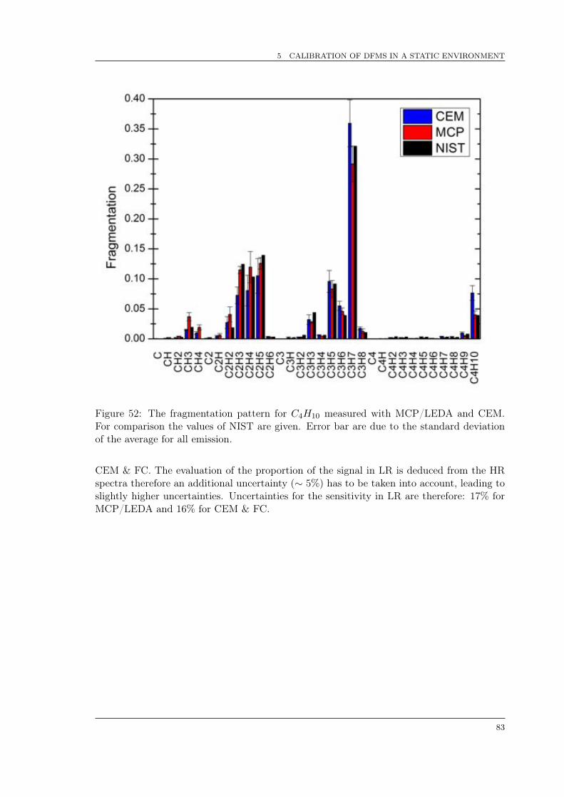
5 CALIBRATION OF DFMS IN A STATIC ENVIRONMENT
Figure 52: The fragmentation pattern for C4H10 measured with MCP/LEDA and CEM.For comparison the values of NIST are given. Error bar are due to the standard deviationof the average for all emission.
CEM & FC. The evaluation of the proportion of the signal in LR is deduced from the HRspectra therefore an additional uncertainty (⇠ 5%) has to be taken into account, leading toslightly higher uncertainties. Uncertainties for the sensitivity in LR are therefore: 17% forMCP/LEDA and 16% for CEM & FC.
83

5 CALIBRATION OF DFMS IN A STATIC ENVIRONMENT
Figure 53: Isotopic abundances of C4H10 relative to literature. The measurements areperformed with an emission of 200 µA for the MCP/LEDA (black) and the CEM (red).The measurements are in good agreement with literature value.
5.9 Alkene
Alkenes are acyclic branched or unbranched hydrocarbons having one carbon-carbon dou-bly bond and the general formula CnH2n [Moss et al., 1995]. The detection of Alkenesin comets was negative so far [Bockelée-Morvan et al., 2004]. However a bunch of hydro-carbons are present in the gas cloud surrounding Rosetta due to spacecraft outgassing[Schläppi et al., 2010], therefore a careful calibration is necessary. Alkenes measurementspresented in this work are only available for Ethylene, other compounds will be part of thestill ongoing calibration campaign for DFMS.
5.9.1 C2H4 Ethylene
The calibration measurements for C2H4 were performed for all detectors and all emissionat one pressure level. The pressure during measurements was 1 x 10�7 mbar and the back-ground pressure before gas inlet was 1 x 10�9 mbar. The pressure measurements are notcorrected because no correction factor was available for the pressure gauge. The pressuremeasurements are therefore relative to N2. A possible correction factor of 0.400 – 0.455 isfound for a similar pressure sensor [Controller, 2001], however since this factor is not givenfor the used pressure sensor a correction was not applied. The measurements were performedwith measurement modes for the MCP/LEDA and CEM, and manually for 28 u/e for theFC.The fragmentation pattern measured with DFMS FM recorded with the MCP/LEDA andCEM can be found in Fig. 54. For comparison the fragmentation found in NIST is given,note that the electron energy for the NIST values is 70 eV, while the electron energy forDFMS is 45 eV and the fragmentation pattern of DFMS is not expected to be the same asthe one given in NIST. The fragmentation presented here is the average of all measurementsfor different emissions. As uncertainties the standard deviation of the average is given.
84

5 CALIBRATION OF DFMS IN A STATIC ENVIRONMENT
Table 24: Sensitivities of DFMS FM for C4H10
Emission MCP/LEDA CEM FCC4H10 Sensitivities for HR [cm3]
200 µA 1.515 x 10�19 3.205 x 10�19 4.611 x 10�19
20 µA 1.946 x 10�19 5.877 x 10�19 N/A2 µA 2.047 x 10�19 7.542 x 10�19 N/A
C4H10 Sensitivities for LR [cm3]200 µA 2.212 x 10�18 6.193 x 10�18 6.860 x 10�18
20 µA 2.037 x 10�18 7.454 x 10�18 7.127 x 10�18
2 µA 1.340 x 10�18 7.518 x 10�18 N/A
Statistical uncertainties are in the same range as the standard deviation, therefore thestandard deviation was used. The fragmentation pattern of DFMS contains more parents,while the fragment C2H3 is depleted compared to NIST, the other fragments are in the samerange or higher than NIST. Differences between MCP/LEDA and CEM can be explainedby differences in the detection efficiencies of the detectors.The evaluation of isotopic abundances was only done for C2H4 since the signal of the isotopesof a fragment due overlap with the heavier fragment and can only be separated if the heavierfragment is less abundant than the isotope. The isotopic abundances measured with DFMSfor C2H4 and C are all in good agreement with literature (see Fig. 55). 13C/12C was mea-sured with the CEM with 200 µA, statistical uncertainties are 20% and dominate the totaluncertainties. The measurements for 13C12CH4/12C2H4 with the MCP/LEDA are given forall emissions. The total uncertainties are dominated by the calibration uncertainties of 5%for the MCP/LEDA and statistical uncertainties are < 1%. 13C2H4/12C2H4 measured withthe MCP/LEDA for all emissions are in agreement with literature. Statistical uncertaintiesare: 200 µA 6%, 20 µA 9%, and 2 µA 18%.The sensitivity was calculated for all detectors and all emissions for DFMS FM (see Tab. 25).The sensitivities are lower for 200 µA and the CEM is more sensitive than the MCP/LEDA.This can be explained by the detection efficiency of the MCP/LEDA, that is lower than forthe CEM for C2H4. The total ion current of C2H4 for the sensitivity contains the signal ofC2H4, the fragments and the isotopes of the parent. Since the pressure measurements arenot corrected, the sensitivities for C2H4 are relative to N2.
Table 25: Sensitivities of DFMS FM for C2H4
Emission MCP/LEDA CEM FCC2H4 Sensitivities for HR [cm3]
200 µA 6.912 x 10�20 1.380 x 10�19 1.493 x 10�19
20 µA 4.490 x 10�19 8.905 x 10�19 7.310 x 10�19
2 µA 6.466 x 10�19 1.300 x 10�18 N/AC2H4 Sensitivities for LR [cm3]
200 µA 7.460 x 10�19 1.596 x 10�18 2.065 x 10�18
20 µA 8.354 x 10�18 1.281 x 10�17 1.370 x 10�17
2 µA 8.260 x 10�18 1.523 x 10�17 1.809 x 10�17
85

5 CALIBRATION OF DFMS IN A STATIC ENVIRONMENT
Figure 54: The fragmentation pattern for C2H4 measured with MCP/LEDA and CEM. Forcomparison the values found in NIST are given. Error bar are due to the standard deviationof the average for all emission.
The statistical error for the sensitivity measurement is < 1%. The uncertainties of the pres-sure measurement are ⇠14% (see App. F). Calibration uncertainties of the MCP/LEDAsuch as gain calibration and individual pixel gain corrections are estimated as ⇠ 7%. Cali-bration uncertainties of the CEM and the FC detector are assumed to be ⇠ 5%. The totaluncertainties for the sensitivity in HR are therefore: 16% for MCP/LEDA and 15% forCEM & FC. The evaluation of the proportion of the signal in LR is deduced from the HRspectra therefore an additional uncertainty (⇠ 5%) has to be taken into account, leading toslightly higher uncertainties. Uncertainties for the sensitivity in LR are therefore: 17% forMCP/LEDA and 16% for CEM & FC.
86

5 CALIBRATION OF DFMS IN A STATIC ENVIRONMENT
Figure 55: The isotopic abundances for C2H4 and C measured with the MCP/LEDA (black)and the CEM (red). All measurements are in good agreement with literature. Error bars arediscussed in the text. For C no measurements are available for the MCP/LEDA, because ofthe limited mass range.
5.10 Minimal densities detectable with DFMS FM and adapted for FS
The detectable density limit of DFMS is important to show DFMS capabilities to detectgas of cometary origin when the comet is not yet very active. Immediately after hibernationof the spacecraft (and far away from the comet) the signal will be dominated by spacecraftoutgassing [Schläppi et al., 2010] but will play a minor role when the comet gets more active.The density is calculated by solving Eq. 15 for the density:
⇢i =Ii
Stotal,i · Iemi(40)
where ⇢i is the number density for neutral species i [cm�3], Ii is the detected current ofthe corresponding ion on the MCP/LEDA or CEM [A], Stotal,i is the sensitivity of speciesi [cm3], and Iemi is the emission current of the filament [A]. To keep the rough estimationas simple as possible the dissociative electron impact ionization from higher mass moleculeson the same m/q signal was neglected.To deduce the minimal density detectable with DFMS, the following settings are chosen tomaximize the signal of this density at the detectors: LR and an emission of 200 µA, becausemore ions can pass the resolution sensitive slit in LR than in HR and more ions get ionizedat the maximum emission. The sensitivities for the FM are lower for an emission of 200µA than for the lower emissions as shown during calibration. However, the sensitivity forthe FS is higher for 200 µA than for the other emissions [Eberhardt, 2008a, Altwegg, 2008a,Eberhardt, 2008b, Altwegg, 2008b], and the minimal density detectable with DFMS mighttherefore be higher for the FM than for the FS.To deduce the minimal signal detected by the detectors the following assumptions are made:
- MCP/LEDA: one ion impinges on the MCP for an integration time of 20 s and the
87

5 CALIBRATION OF DFMS IN A STATIC ENVIRONMENT
resulting signal is detected by the LEDA (according to Eq. 18 this is a signal of ⇠ 150counts on GS 16).
- CEM: five ions during an integration time of 1 s (according to Eq. 34 this is a signalof 1 count in LR).
To get an overview of the detection limits of the calibrated species, they are listed in Tab.26:
Table 26: Minimal densities detectable by DFMS FM
Species Density MCP/LEDA [cm�3] Density CEM [cm�3]Ne 33 ± 5 3419 ± 547Ar 10 ± 2 493 ± 79Kr 62 ± 10 633 ± 101Xe 117 ± 19 399 ± 64H2O 8 ± 1 1237 ± 198N2 8 ± 1 716 ± 115CO2 19 ± 3 725 ± 116CH4 3 ± 1 313 ± 50C2H6 15 ± 2 817 ± 131C3H8 29 ± 5 740 ± 118C4H10 18 ± 3 657 ± 105C2H4 54 ± 9 2559 ± 409
The detection limits for the MCP/LEDA are much lower than for the CEM. However, thenominal integration time of the MCP/LEDA is 20 s and therefore a factor of 20 higher thanfor the CEM. The detection limit can be further reduced by addition of several spectra andtherefore a higher total integration time. The minimal densities of these species detected bythe FS will be higher because of the higher sensitivity for 200 µA and can be used as upperlimits of the minimal density required to be detectable by DFMS FS. Also the detectionlimit for water is harmed by the spacecraft surrounding background cloud due to outgassing(see Schläppi et al. (2010)).The required sensitivity given in Balsiger et al. (2007) of 10�5 A/mbar correlates with asignal of 1 ion detected in 500 s for a density of 1 cm�3 and an emission of 10 µA and meetsthe here presented signal of one ion in 20 s for an emission of 200 µA. The sensitivity forthis condition calculated according to Eq. 15 is ⇠ 1 x 10�17 cm3. This sensitivity could beroughly reproduced with the FM for the following species in LR: Ar, H2O, N2, CH4, andC2H6.
88

6 ANALYSIS OF GAS MIXTURE
6 Analysis of gas mixture
In this chapter different gas mixtures are analyzed to show the quality of the calibrationmeasurements. This chapter presents the most difficult part of the data analysis; wheresignal is first identified, transformed into ion current, and ultimately resulting in deductionof partial and total densities. DFMS FS can measure relative densities at the comet andCOPS FS measurements will be used to translate into accurate total densities. The intentis to show DFMS capabilities immediately after hibernation as the first measurements willutilize the settings used for the measurements in this section (MCP/LEDA, HR, and 200µA). Three gas mixtures were analyzed:
• GCU gas a mixture of Ne, Xe and CO2
• Noble gas mixture containing Ne, Ar, Kr, and Xe
• Gas mixture containing CO2 and C3H8
The measurement procedure was the same as for the calibration campaign (see Sec. 5.2).
6.1 Data treatment
The lab environment has the advantage that the measured species are known and thereforethe data analysis is biased by this knowledge. It is clearly known if a species is a fragmentor the parent itself. The situation for the FS and therefore the analysis of the data isdifferent. The measured mixture at the comet will be dominated by the background due tospacecraft outgassing as the comet will not yet be very active (directly after hibernation ofthe spacecraft). Although the background is mainly dominated by water, a lot of differentspecies were detected before hibernation [Schläppi et al., 2010]. These species will likely stillbe detectable after hibernation, but should be of the same order of magnitude or less. Oncethe comet becomes active and the spacecraft is close, the detected signal should then bedominated by outgassing of the comet. Once a signal is identified as the signal of species i,the total density can be calculated by the following (i can be a fragment, the parent or anisotope):
⇢total,i =Ii
Stotal,i
1
fi
1
Iemi(41)
Where ⇢total,i is the total density for i [cm�3] including the density of all the fragments andisotopes. Ii is the measured ion current for i [A], Stotal,i is the total sensitivity for i [cm3],fi is the factor of the fragmentation pattern or the isotopic abundance (if known) and Iemi
is the emission current [A]. Ii is calculated as described for the MCP/LEDA in Eq. 18 andfor the CEM in Eq. 34. The MCP/LEDA data was treated as described in Sec. 4.3.The partial density of i can be calculated the following:
⇢i =Ii
Stotal,i
1
Iemi(42)
The partial density of i does not need to be corrected for a fragmentation pattern, since theion currents can be directly interpreted as the partial density of i.
89

6 ANALYSIS OF GAS MIXTURE
6.2 Possible approach
Identification of parent molecules and the composition analysis requires a complex approach.The data analysis process involves an informed correlation of the signal in the spectra ofeach individual mass to identify parents, fragments and isotopes. The best way to findthe parents is to start at the heaviest masses. Species that are known to be measuredsuch as H2O, CO2, and the GCU-component gases, help to determine the mass scales ofeach spectrum and therefore the range of p0. Since the mass range of DFMS is limited,comparisons with RTOF for heavier species will help to identify heavy molecules and thepossible fragments thereof. Once a parent is identified, the fragmentation pattern of thismolecule can be subtracted and with the remaining signal one can proceed. To check if theidentification of a signal is adequate, the spectra of the isotopes and the fragments must alsobe taken into account. If the fragments or isotopes are not available or their abundancesdo not adequately match the data, the signal might be incorrectly identified. Because theisotopic abundances in the coma of the comet are not necessarily expected to be in agreementwith Earth abundances they must be handled carefully.To get an overview of the total mass range, the ion currents for every spectrum can beplaced together according to their mass.
6.3 GCU gas: Ne+CO2+Xe
Figure 56: MCP/LEDA measurement in HR with an emission of 200 µA for the GCU gas.The GCU contains Ne, CO2 and Xe. The peaks around 66 u/e are the signal of the doublycharged Xe. The signal of O and CO are the fragments of CO2.
The gas in the GCU of DFMS contains mainly CO2, Ne and Xe. The mixture was chosento contain 90% CO2, 9% Ne and 0.9% Xe and 0.1% He of the volume. The description ofthe bottle containing the same GCU gas as used to fill the GCU can be found in Tab. 27.
90

6 ANALYSIS OF GAS MIXTURE
Table 27: Description of the GCU gas mixture.
Species Ratio of Relative ratio Relative ratio Bottle rel. deviationVolume [%] of Volume [%] of weight [%] description [%] [%]
CO2 100 90.1 92.886 91.938 (rest) 2Ne 10 9.0 4.260 4.490 2Xe 1 0.9 2.845 2.574 2He 0 0.1 0.009 0.998 2
The GCU gas is directly introduced into the ion source of DFMS. The pressure outside of theion source was 1.0 x 10�7 mbar (no correction applied). This pressure is expected to be lowerthan the actual pressure inside the ion source, since the gas is introduced directly into the ionsource. The calibration measurements for CO2, Ne, and Xe can now be used to calibratethe pressure inside the ion source for GCU measurements. For the GCU measurements thereexist special measurement modes. In these modes the masses 44, 45, 28, 22, 20, 16, 64, 65,66 (only in HR), 68, 129, 132 (only in HR), 136, and 44 again are commanded. Thereforethe isotopic measurements are limited. To reduce measurement time for the MCP/LEDAthe total integration time of this modes is 66 ms and 150 accumulations, resulting in a totalintegration time of 9.9 s. The measurements presented are recorded with the MCP/LEDAat HR and an emission setting of 200 µA.
Table 28: Fragmentation of the GCU gas for CO2 measured with the MCP/LEDA in HRfor an emission of 200 µA.
Species Fragmentation Total uncertainties Fragmentation Standardmeasured [%] calibrated deviation
16O 0.110 5 0.121 0.01412C16O 0.105 5 0.099 0.00612C16O2 0.784 5 0.779 0.016
The fragmentation pattern for CO2 in the GCU gas is given in Tab. 28. For comparisonthe calibrated fragmentation pattern for CO2 is given with the standard deviation as un-certainties. The fragmentation behavior for CO2 in the GCU gas is in good agreement withthe calibrated fragmentation. Total uncertainties for CO2 in the GCU gas is given by thecalibration error of the MCP/LEDA and the statistical uncertainties (<1%).
91
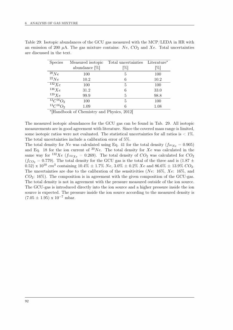
6 ANALYSIS OF GAS MIXTURE
Table 29: Isotopic abundances of the GCU gas measured with the MCP/LEDA in HR withan emission of 200 µA. The gas mixture contains: Ne, CO2 and Xe. Total uncertaintiesare discussed in the text.
Species Measured isotopic Total uncertainties Literature⇤abundance [%] [%] [%]
20Ne 100 5 10022Ne 10.2 6 10.2132Xe 100 5 100136Xe 31.2 6 33.0129Xe 99.9 5 98.812C16O2 100 5 10013C16O2 1.09 6 1.08⇤[Handbook of Chemistry and Physics, 2012]
The measured isotopic abundances for the GCU gas can be found in Tab. 29. All isotopicmeasurements are in good agreement with literature. Since the covered mass range is limited,some isotopic ratios were not evaluated. The statistical uncertainties for all ratios is < 1%.The total uncertainties include a calibration error of 5%.The total density for Ne was calculated using Eq. 41 for the total density (f20Ne = 0.905)and Eq. 18 for the ion current of 20Ne. The total density for Xe was calculated in thesame way for 132Xe (f132Xe = 0.269). The total density of CO2 was calculated for CO2
(fCO2 = 0.779). The total density for the GCU gas is the total of the three and is (1.87 ±0.52) x 1010 cm3 containing 10.4% ± 1.7% Ne, 3.0% ± 0.2% Xe and 86.6% ± 13.9% CO2.The uncertainties are due to the calibration of the sensitivities (Ne: 16%, Xe: 16%, andCO2: 16%). The composition is in agreement with the given composition of the GCU-gas.The total density is not in agreement with the pressure measured outside of the ion source.The GCU-gas is introduced directly into the ion source and a higher pressure inside the ionsource is expected. The pressure inside the ion source according to the measured density is(7.05 ± 1.95) x 10�7 mbar.
92

6 ANALYSIS OF GAS MIXTURE
6.4 Noble gas mixture: Ne–Ar–Kr–Xe
Figure 57: Measurement of a gas mixture containing Ne, Ar, Kr, and Xe measured withthe MCP/LEDA in HR at an emission of 200 µA. The peaks marked as Xe are due to thedoubly charged Xenon.
The measurements of the gas mixture with Ne, Ar, Kr, and Xe are performed at a measuredpressure of 1 x 10�7 mbar (no correction applied). The background pressure was 5 x 10�9
mbar. The gas mixture is a bottle containing 25% of the molecules of each gas. A spectrumof the total mass range for this mixture is given in Fig. 57. The measurements are recodedwith nominal scan modes, therefore the mass range of the HR mode does not cover the massof Xe but the doubly charged Xenon. Since all the detected ions were originally neutralsand measurements were performed in the neutral mode, the charge state of the atoms is notindicated. The background measurements are already subtracted, therefore neither H2Onor CO2 are visible.
The measured isotopic abundances for the mixture can be found in Tab. 30. All themeasurements are in good agreement with literature value. The total uncertainties containthe calibration uncertainties of the MCP/LEDA (5%) and the statistical uncertainties. Withthe exception of 126Xe and 124Xe the total uncertainties are dominated by the calibrationuncertainties.
93

6 ANALYSIS OF GAS MIXTURE
Table 30: Isotopic abundances of the gas mixture measured with the MCP/LEDA in HR withan emission of 200 µA. The gas mixture contains: Ne, Ar, Kr, and Xe. Total uncertaintiesare discussed in the text.
Species Measured isotopic Total uncertainties Literature⇤abundance [%] [%] [%]
20Ne 100 5 10021Ne 0.30 7 0.3022Ne 10.7 5 10.240Ar 100 5 10038Ar 0.06 6 0.0636Ar 0.36 5 0.3484Kr 100 5 10086Kr 30.2 5 30.383Kr 20.3 5 20.282Kr 20.2 5 20.380Kr 4.00 5 4.0178Kr 0.62 5 0.62132Xe 100 5 100136Xe 32.5 6 33.0134Xe 38.4 6 38.8131Xe 79.7 5 78.8130Xe 14.8 6 15.2129Xe 97.6 5 98.8128Xe 7.09 7 7.14126Xe 0.33 16 0.35124Xe 0.32 16 0.35⇤[Handbook of Chemistry and Physics, 2012]
The total density for Ne was calculated by the sum of the partial density using Eq. 42for every isotope and the sensitivity of the MCP/LEDA for 200 µA in Tab. 13. The ioncurrent for every isotope was calculated according to Eq. 18. The total densities for Ar andKr are calculated in the same way with the corresponding sensitivities (Ar: Tab. 14 andKr: Tab. 15). The sensitivity for Xe in Tab. 16 was corrected for the doubly charged Xewith a factor of 0.013 (1.3%). The total density is then calculated in the same way as forthe other noble gases. The total measured density for the mixture is 3.45 x 109 cm�3 andcontains; 13% ± 2% Ne, 24% ± 4% Ar, 26%± 4% Kr, and 37% ± 5% Xe. The measuredpressure of 1.08 x 10�7 mbar is corrected with the average of all the correction factors (forcorrection factors see App. F), since the ratio of every gas should be the same. The totaldensity measured with DFMS is in good agreement with the total density deduced fromthe pressure measurements of 3.56 x 109 cm�3. The uncertainties are dominated by theuncertainties of the sensitivities of 16%, however the difference between the total densitiesis only 3.1%. The composition of the mixture is not in agreement with the expected 25%for every compound. A possible reason for the difference could be found in the setup forstatic measurements. Since the pumps are always running while the amount of pumped gasis compensated by the inlet of the gas, this is not a completely static environment. Thepumping efficiency for the different compounds has an influence on the relative composition
94

6 ANALYSIS OF GAS MIXTURE
of the measured gas. Ne is much easier to pump than Xe. This was observed during thecalibration campaign, since the contamination of the background measurements after thecalibration of Xe was much higher then for Ne. Ne disappears almost immediately afterthe gas inlet is closed, it must therefore be much easier to pump. This might not be theonly explanation but seems appropriate. An other explanation could be that the calibrationof the sensitivities is not in the expected quality. But this can be negotiated since the sameeffect is also detected in the measurements with LR and for other emissions.
95

6 ANALYSIS OF GAS MIXTURE
6.5 CO2+C3H8
Figure 58: MCP/LEDA measurement in HR with an emission of 200 µA for the CO2 +C3H8 mixture. HR spectra with a better resolution of the three highlighted peaks can befound in Fig. 59. For a better overview the other fragments of C3H8 are not highlightedbut can be found in Tab. 32.
The measurements of the gas mixture containing CO2 + C3H8 are performed at a measuredpressure of 8.9 x 10�7 mbar (no correction applied). The background pressure was 6.8 x10�10 mbar. The gas mixture was produced through the flow controller of CASYMIR inthe GMU (see Sec. 5.1). To control the gas inlet one gas after the other was introducedinto the GMU and the GMU was still pumped. When the pump was switched off, the GMUwas filled with ⇠50% CO2 and ⇠50% C3H8. The gas was then introduced from the GMUinto the chamber at the leak valve (LV4) used for the static calibration. The measurementsfor the MCP/LEDA with an emission of 200 µA are recorded with scan modes covering themass range of 13 u/e – 50 u/e. The complete mass scan in HR of the mixture recordedwith the MCP/LEDA at an emission of 200 µA can be found in Fig. 58. The peaks weresignals of both gases can be found are highlighted and the composition is indicated. To showthe capability of DFMS to resolve these peaks, spectra of 16 u/e, 28 u/e, and 44 u/e in alogarithmic scale are given in Fig. 59. Background measurements are carefully subtracted,therefore no signal of N2 is found on the spectrum of 28 u/e.
96

6 ANALYSIS OF GAS MIXTURE
Figure 59: The three spectra of the fragments and the parent molecule of both gases.MCP/LEDA measurement in HR with an emission of 200 µA for the CO2 + C3H8 mixture.
Table 31: Fragmentation of the gas mixture for CO2 measured with the MCP/LEDA in HRfor an emission of 200 µA.
Species Fragmentation Total uncertainties Fragmentation Standardmeasured [%] calibrated deviation
16O 0.119 5 0.121 0.01412C16O 0.091 5 0.099 0.00612C16O2 0.775 5 0.779 0.016
The fragmentation pattern for the gas mixture of CO2 + C3H8 can be found in Tab. 31for CO2 and Tab. 32 for C3H8. For comparison the calibrated fragmentation pattern ofthe calibration campaign is given and the standard deviation as uncertainties. The totaluncertainties of the fragmentation pattern of the gas mixture contain the statistical uncer-tainties and the calibration uncertainties for the MCP/LEDA. The fragmentation behaviorof CO2 is in good agreement with the calibrated fragmentation. The fragmentation ratioof 12C3H, 12C3H5, and 12C3H6 for C3H8 are not in agreement with the calibration. Anexplanation could be that the most present fragment 12C2H5 has total uncertainties of 5%and can therefore deviate 0.014, this has an influence on the other fragments ratios. Toshow the impact of the statistical uncertainties, the total uncertainties does not take intoaccount this variation. In summary the fragmentation behavior of CO2 and C3H8 duringthe calibration could be reproduced in this gas mixture.
97

6 ANALYSIS OF GAS MIXTURE
Table 32: Fragmentation of the gas mixture for C3H8 measured with the MCP/LEDA inHR for an emission of 200 µA.
Species Fragmentation Total uncertainties Fragmentation Standardmeasured [%] calibrated deviation
12CH 0.002 5 0.002 0.00012CH2 0.008 5 0.007 0.00212CH3 0.041 5 0.044 0.00812CH4 0.018 5 0.016 0.00712C2 0.001 6 0.001 0.00012C2H 0.004 5 0.004 0.00112C2H2 0.042 5 0.041 0.00112C2H3 0.128 5 0.128 0.02212C2H4 0.194 5 0.198 0.01812C2H5 0.285 5 0.277 0.02612C3 0.000 17 0.000 0.00012C3H 0.003 5 0.002 0.00012C3H2 0.007 5 0.007 0.00112C3H3 0.040 5 0.042 0.01412C3H4 0.007 5 0.006 0.00112C3H5 0.032 5 0.035 0.00212C3H6 0.010 5 0.013 0.00112C3H7 0.072 5 0.074 0.00712C3H8 0.100 5 0.098 0.004
The isotopic ratios for the gas mixture containing CO2 and C3H8 can be found in Tab.33. All isotopic ratios are in agreement with literature. The total uncertainties take intoaccount the calibration uncertainties of the MCP/LEDA (5%) and statistical uncertainties.The statistical uncertainties of the isotopes are: 4% for 13C16O, 3% for 13C16O2, 3% for13C12CH5, and 4% for 13C12C2H8.
Table 33: Isotopic abundances of the gas mixture with the MCP/LEDA in HR at an emissionof 200 µA. The gas mixture contains: CO2 and C3H8. Total uncertainties are discussed inthe text.
Species Measured isotopic Total uncertainties Literature⇤abundance [%] [%] [%]
12C16O 100 5 10013C16O 1.05 7 1.0812C16O2 100 5 10013C16O2 1.05 6 1.0812C2H5 100 5 10013C12CH5 2.03 6 2.1612C3H8 100 5 10013C12C2H8 3.11 7 3.24⇤[Handbook of Chemistry and Physics, 2012]
98

6 ANALYSIS OF GAS MIXTURE
The total density for CO2 was calculated for CO2 using Eq. 41 and the sensitivity of Tab.20. For fCO2 the calibrated fragmentation ratio for CO2 in Tab. 31 was used. The totaldensity for CO2 is (1.04 ± 0.17) x 109 cm�3. The total uncertainties are dominated by thecalibration uncertainties of the sensitivity of 16%. The total density for C3H8 was calculatedfor C3H8 in the same way and is (1.18 ± 0.19) x 109 cm�3. The total density for the gasmixture is then (2.22 ± 0.36) x 109 cm�3 containing 47% ± 8% CO2 and 53% ± 8% C3H8.The pressure measurements are (7.0 ± 1.2) x 10�8 mbar. The pressure measurements arecorrected with the average of the corrections factors for CO2 and N2, since the ratio forboth gases is the same and C3H8 sensitivities are given relative to N2 (for explanation seeSec. 5.8.3). The uncertainties of the pressure measurements are 14%. The resulting densityis then (2.0 ± 0.28) x 109 cm�3. The total density of the gas mixture is in good agreementwith the density of the pressure measurements.
99

6 ANALYSIS OF GAS MIXTURE
100

7 CONCLUSION AND OUTLOOK
7 Conclusion and outlook
The goal of this work was to further improve the knowledge about the peculiarities of DFMS,the instrument handling with GSEOS, to improve the knowledge about the data analysisand the handling of technical problems is achievable. This part is intended as a brief con-clusion and outlook of this work, concerning DFMS, the characteristics, the calibration, andthe evaluation of measured gas mixtures.
DFMS characteristics:
The characterization of the instrument contains: ionization and fragmentation behavior inthe ion source, instrument transmission and detection efficiency. Furthermore a detaileddescription of the data analysis to transform the signal into an ion current is given.The sensitivity of an instrument depends on the ionization efficiency in the ion source,the instrument transmission and the detection efficiency. The ionization in the ion sourcefor different electron energies confirmed the most efficient ionization for an electron energyof 45 eV as expected from the work in Schläppi (2011). The fragmentation behavior ofthe ion source of DFMS depends strongly on the electron energy and can therefore bemanipulated to suppress (22 eV) or force (70 eV) fragmentation. The transmission of theinstrument depends on the resolution of the instrument because of the ion path throughthe instrument and goes roughly with 1/m. The sensitivity then is the combination ofthe ionization efficiency, the fragmentation behavior, the instrument transmission and thedetection efficiency. An absolute calibration of each of these characteristics is not feasiblesince the sensor is operated as a total an therefore the sensitivity is the combination of thesecharacteristics. However, e.g. the ratio of the detection efficiencies of the MCP/LEDArelative to the CEM can be deduced and is necessary to deduce sensitives of species wherea calibration was not realizable.The characteristics for the FM can be adapted to the FS with the exception of the ionizationefficiency of the different emission currents of the filament. The ionization efficiency of theFM for an emission current of 200 µA is less than a factor of 10 compared to 20 µA, but forthe FS the factor is > 10. However, since the FS is on the spacecraft the influence of thiseffect can be used in a beneficial way, although the physical effect is not understood by theauthor.
Calibration of DFMS in a static environment:
The calibration was performed for several species (see Tab. 34) and the results for isotopicratios mostly confirm literature values[Handbook of Chemistry and Physics, 2012]. The sen-sitivity of DFMS FM for this species, was calibrated and the fragmentation behavior mea-sured.The linear behavior of the signal measured by DFMS and the density of the gas couldbe reproduced for Ne and Ar and is therefore expected for the other species as well. Thequality of the calibration of the fragmentation pattern is difficult to set in context with othermeasurements and instruments as found in NIST, since the electron energy in the ion sourceis reduced (DFMS: 45 eV and NIST: 70 eV). However, the tendency that the fragmentationis lower for lower energies and higher for higher electron energies has been shown. Thecalibration campaign presented in this work as well as further calibration measurements
101

7 CONCLUSION AND OUTLOOK
Table 34: The gases used for calibration of DFMS and references for tables.
Species Tab. of Tab. of fragmentation Tab. of fragmentationSensitivities pattern MCP pattern CEM
Ne 13 MCP/LEDA: None CEM: NoneAr 14 MCP/LEDA: None CEM: NoneKr 15 MCP/LEDA: None CEM: NoneXe 16 MCP/LEDA: None CEM: NoneH2O 18 MCP/LEDA: E.4 CEM: E.3N2 19 MCP/LEDA: E.6 CEM: E.5CO2 20 MCP/LEDA: E.8 CEM: E.7CH4 21 MCP/LEDA: E.10 CEM: E.9C2H6 22 MCP/LEDA: E.12 CEM: E.11C3H8 23 MCP/LEDA: E.14 CEM: E.13C4H10 24 MCP/LEDA: E.16 CEM: E.15C2H4 25 MCP/LEDA: E.18 CEM: E.17
will provide fragmentation pattern for DFMS although a confirmation of the fragmentationpattern in NIST could have reduced the calibration measurements.To compare the sensitivities of the calibration with earlier calibrations, the sensitivitiesin this work are transferred into a slope. The slope for Ne (20 µA) measured with theMCP/LEDA given in Riesen (2007) is 1.14 x 10¹² for LR and 1.14 x 10¹¹ for HR. The slopecalculated as defined in Riesen (2007) for the Ne calibration in this work and for an emissionof 20 µA is 4.77 x 10¹² for LR and 2.13 x 10¹¹ for HR. The slope represents the sensitivityover different pressure ranges. A higher slope means that the signal detected relative tothe pressure was higher and therefore the sensitivity of the instrument. The sensitivity ofDFMS FM for Ne has improved since the work of Riesen (2007). A possible explanationcould be that the gain of the MCP was recalibrated or that the pixel gain correctionswere consequently applied in this work, while Riesen (2007) tried to avoid this correctionby shifting the maximal signal on the same pixel. The more likely reason however mightbe that between this work and Riesen (2007), the instrument was optimized by Schläppi(2011). The optimization was necessary to describe the sensor and its setting as total and ina physical manner and not only to find optimized settings to record one spectra for a smallmass range.The required sensitivity given in Balsiger et al. (2007) of 10�5 A/mbar correlates with asignal of 1 ion detected in 500 s for a density of 1 cm�3 and an emission of 10 µA. Thesensitivity for this conditions calculated according to Eq. 15 is ⇠ 1 x 10�17 cm3. DFMS FMdoes meet that requirement for the MCP/LEDA for the following species of the calibrationin LR: Ar, H2O, N2, CH4, and C2H6. It is known for the FS that the sensitivity for anemission of 200 µA is higher than for the other emissions. With the assumption that the FSis as sensitive as the FM for 20 µA and 2 µA, the list of species that meet the requirementgiven in Balsiger (2007) might even be enlarged.
The calibration campaign should be continued with other gases (e.g. CO, O2) and othersolid or liquid compounds that are expected to be found in comets or the spacecraft sur-rounding cloud. A detailed list of postulated and detected species in the coma of comets
102
7 CONCLUSION AND OUTLOOK
can be found in Bockelée-Morvan et al. (2004). To introduce the gaseous phase of thesecompounds the gas inlet of CASYMIR should be further improved so that compounds canbe heated in a controlled way and the gaseous phase introduced into the chamber.
Analysis of gas mixtures:
The three gas mixtures that were analyzed are the following: GCU-gas with Ne+Xe+CO2,noble gas mixture with Ne+Ar+Kr+Xe, and CO2+C3H8. They were evaluated accordingto the calibration values found during the calibration campaign and are a test for the qualityof the calibration. Although the set of mixtures was rather small and the evaluation wasfocused on the measurements of the MCP/LEDA, the expected densities and ratios of themixture are in good agreement with the measurements of DFMS FM. However, mixtures ofgases, where the fragment of one gas is detected on the same peak as the parent moleculeof the other gas (CO and CO2) might then show the real quality of the calibration of thefragmentation pattern and the sensitivities. Other interesting mixtures to measure are thecombination of H2O and CO2. Therefore the calibration facility (CASYMIR) should befurther improved to produce mixtures of different phases like H2O and CO2 in a controlledway and introduce them into the chamber. The calibration of the GCU-gas density insidethe ion source is important to compare measurements of the FS with the FM.
The software to control the settings of the voltages and modes of DFMS is in a very stablecondition so that the instrument can be operated over nights and weekends without minorerrors. However, the stability of the software will only be confirmed if all three sensors(DFMS, RTOF and COPS) can measure at the same time, while commanded from the sameDPU and over a long time range without any failures. Therefore additional software testsof all three sensors are planned.
103


Appendix
Appendix
105

A SPICE SOLAR ASPECT ANGLE (SAA)
A SPICE Solar Aspect Angle (SAA)
****************************************************************************
SPICE code in c to extract the Solar Aspect Angle (SAA) of Rosettafor the Lutetia flyby
****************************************************************************
---------------------------------kernel input-------------------------------RO_kernels.tm contains the kernel input in the following order:
ck: ATNR_P040302093352_00116.BCfk: EARTH_TOPO_050714.TFfk: EARTHFIXEDITRF93.TFfk: NEW_NORCIA_TOPO.TFfk: ROS_V16.TFfk: RSSD0002.TFik: ROS_ROSINA_V11.TIlsk: NAIF0009.TLSpck: DE403-MASSES.TPCpck: EARTH_000101_110304_101211.BPCpck: PCK00008.TPCsclk: ROS_101110_STEP.TSCspk: ORHR_______________00109.BSPspk: DE405.BSPspk: ROS_STRUCT_V2.BSP
The following kernels should be updated if the time range does not match thetime range of the kernels:
ck: ATNR_P040302093352_00116.BCpck: EARTH_000101_110304_101211.BPCspk: ORHR_______________00109.bsp
Time ranges for these kernels:ATNR_P040302093352_00116.BCObject: -226000Interval Begin ET Interval End ET AV------------------------ ------------------------ ---2004-MAR-02 09:33:52.767 2011-MAR-31 01:01:06.183 Y
EARTH_000101_110304_101211.BPC
106

A SPICE SOLAR ASPECT ANGLE (SAA)
Frame: ITRF93 (3000)Start of Interval (ET) End of Interval (ET)----------------------------- -----------------------------2000 JAN 01 00:01:04.183 2011 MAR 05 00:01:06.185
ORHR_______________00109.bspBody: ROSETTA (-226)Start of Interval (ET) End of Interval (ET)----------------------------- -----------------------------2004 MAR 02 09:26:21.583 2014 MAY 23 01:43:30.120-----------------------------------------------------------------------------
-------------------------------C-code----------------------------------------
#include <stdio.h>#include <string.h>#include "SpiceUsr.h"
#define METAKR "RO_kernels.tm"
#define SCLKID -226 // Cassini NAIF ID (aus naif_ids.html) -226 for ROSETTA#define STRLEN 50 // Lenght of utctim +1!
int main (void){
SpiceChar utctim [STRLEN];SpiceChar utctim_start [STRLEN];SpiceChar utctim_end [STRLEN];SpiceChar start [STRLEN];SpiceChar filename [STRLEN];
SpiceDouble angle_radx;SpiceDouble angle_rady;SpiceDouble angle_radz;SpiceDouble angle_degx;SpiceDouble angle_degy;SpiceDouble angle_degz;SpiceDouble state [6];SpiceDouble rosx [3];SpiceDouble rosy [3];SpiceDouble rosz [3];
107

A SPICE SOLAR ASPECT ANGLE (SAA)
SpiceDouble et_start;SpiceDouble et_end;SpiceDouble et;SpiceDouble ltime;SpiceDouble delta;
SpiceDouble pos [3];SpiceDouble dist_km;SpiceDouble dist_au;
SpiceDouble step;SpiceDouble imax;
FILE *solar_angle;
furnsh_c ( METAKR );
// get UTC time to extract SAAprompt_c( "Input UTC Start-Time (2010-02-18T12:00:00): ",
STRLEN, utctim_start );prompt_c( "Input UTC End-Time (2010-02-18T22:00:00): ",
STRLEN, utctim_end );
printf( "Converting UTC Start-Time: %s\n", utctim_start );printf( "Converting UTC End-Time: %s\n", utctim_end );
strncpy (start, utctim_start, 10);sprintf( filename , "solarangle-%s.dat" , start );
solar_angle = fopen ( filename ,"w"); // w :write
// Print used kernels in *.xls filefprintf(solar_angle,"The loaded Kernels are:\n %s\n %s\n %s\n %s\n %s\n %s\n
%s\n %s\n %s\n %s\n %s\n %s\n %s\n %s\n %s\n\n","kernels/ck/ATNR_P040302093352_00116.BC",
"kernels/fk/EARTH_TOPO_050714.TF","kernels/fk/EARTHFIXEDITRF93.TF","kernels/fk/NEW_NORCIA_TOPO.TF","kernels/fk/ROS_V16.TF","kernels/fk/RSSD0002.TF","kernels/ik/ROS_ROSINA_V11.TI","kernels/lsk/NAIF0009.TLS",
108

A SPICE SOLAR ASPECT ANGLE (SAA)
"kernels/pck/DE403-MASSES.TPC","kernels/pck/EARTH_000101_110304_101211.BPC","kernels/pck/PCK00008.TPC","kernels/sclk/ROS_101110_STEP.TSC","kernels/spk/ORHR_______________00109.BSP","kernels/spk/DE405.BSP","kernels/spk/ROS_STRUCT_V2.BSP");
fprintf(solar_angle,"%s\t %s\t %s\t %s\t %s\n","UTC [YYYY-MM-DDTHH:MM:SS]","Solar angle x [deg]","Solar angle y [deg]", "Solar angle z [deg]","Solar Distanz [AU]");
// Convert start and end time into ETutc2et_c( utctim_start, &et_start );utc2et_c( utctim_end, &et_end );
// Time step to extract SAA in s (300 s = 5 min)step = 300;imax = (et_end - et_start)/step;
// Extract position vector (x,y,z) of the Sun in the Rosetta frame from kernelsint i;for ( i=0; i< imax ;i++){et = (et_start + step*i);
if( et < et_end ){spkezr_c( "SUN", et, "ROS_SPACECRAFT", "NONE", "ROSETTA", state, <ime);
rosx[0] = 1;rosx[1] = 0;rosx[2] = 0;
rosy[0] = 0;rosy[1] = 1;rosy[2] = 0;
rosz[0] = 0;rosz[1] = 0;rosz[2] = 1;
// Convert angle from rad to degrees for every vector
109

A SPICE SOLAR ASPECT ANGLE (SAA)
angle_radx = vsep_c ( state, rosx );convrt_c ( angle_radx, "RADIANS", "DEGREES", &angle_degx);
angle_rady = vsep_c ( state, rosy );convrt_c ( angle_rady, "RADIANS", "DEGREES", &angle_degy);
angle_radz = vsep_c ( state, rosz );convrt_c ( angle_radz, "RADIANS", "DEGREES", &angle_degz);
// Extract heliocentric distance of Rosetta relative to the Sunpos [0] = state [0];pos [1] = state [1];pos [2] = state [2];
// Convert distance from km to AU
dist_km = vnorm_c ( pos );convrt_c ( dist_km, "KM", "AU", &dist_au );
}
// Convert time stamp of the data in s back to UTCet2utc_c ( et, "ISOC",0,STRLEN,utctim);
// Print time stamp in UTC, angle (x,y,z), distance to the Sunfprintf(solar_angle,"%s\t %20.6f\t %20.6f\t %20.6f\t %20.6f\n" ,utctim , angle_degx , angle_degy, angle_degz, dist_au );
}fclose ( solar_angle );return 0;}
110

B SPICE: TRAJECTORIES
B SPICE: Trajectories
****************************************************************************
SPICE code in c to extract the position of Rosetta relative to 67Pfor bound orbits for planing purposes
****************************************************************************
---------------------------------kernel input-------------------------------Chury-trajectory.tm contains the kernel input in the following order:
fk: ROS_V17.TFlsk: NAIF0010.TLSpck: PCK00010.TPCpck: ROS_CGS_RSOC_V03.TPCsclk: ROS_101110_STEP.TSCspk: roviz_t104_p000_c000_s000_g000_r003_a0_v000.bspspk: ORHW_______________00016.BSPspk: DE405.BSP
The trajectory kernels should be updated if the time range does not match:
spk: roviz_t104_p000_c000_s000_g000_r003_a0_v000.bsp
Time range:Body: ROSETTA (-226)
Start of Interval (ET) End of Interval (ET)----------------------------- -----------------------------2014 DEC 01 00:01:06.183 2015 FEB 01 00:01:06.183
-----------------------------------------------------------------------------
-------------------------------C-code----------------------------------------
#include <stdio.h>#include <string.h>#include "SpiceUsr.h"
#define METAKR "Chury-trajectory.tm"#define SCLKID -226 // Cassini NAIF ID (aus naif_ids.html) -226 for ROSETTA#define STRLEN 50 // Lenght of utctim +1!
111

B SPICE: TRAJECTORIES
int main (void){
SpiceChar utctim [STRLEN];SpiceChar utctim_start [STRLEN];SpiceChar utctim_end [STRLEN];SpiceChar start [10];SpiceChar end [10];SpiceChar filename [44];
SpiceDouble state [6];SpiceDouble et_start;SpiceDouble et_end;SpiceDouble et;SpiceDouble ltime;
SpiceDouble pos [3];SpiceDouble dist_m;
SpiceDouble step;SpiceDouble imax;
FILE *chury_trajectory;
furnsh_c ( METAKR );
// Give start and end timestrncpy(utctim_start, "2014-12-01T01:00:00", STRLEN);strncpy(utctim_end, "2014-12-31T00:00:00", STRLEN);strncpy (start, utctim_start, 10);strncpy (end, utctim_end, 10);
sprintf( filename , "%s-%s-chury_trajectory.dat" , start, end);chury_trajectory = fopen ( filename ,"w"); // w :write
// Print used kernels in *.xls filefprintf(chury_trajectory,"The loaded Kernels are:\n %s\n %s\n %s\n %s\n %s\n %s\n %s\n %s\n\n","kernels/fk/ROS_V17.TF",
"kernels/lsk/NAIF0010.TLS","kernels/pck/PCK00010.TPC","kernels/pck/ROS_CGS_RSOC_V03.TPC","kernels/sclk/ROS_101110_STEP.TSC",
112

B SPICE: TRAJECTORIES
"kernels/spk/roviz_t104_p000_c000_s000_g000_r003_a0_v000.bsp","kernels/spk/ORHW_______________00016.BSP","kernels/spk/DE405.BSP");
// Convert start and end time into ETutc2et_c( utctim_start, &et_start );utc2et_c( utctim_end, &et_end );
// Time step to extract position in s (300 s = 5 min)step = 3600;
imax = (et_end - et_start)/step;fprintf(chury_trajectory, "Start time UTC: %s\t End time UTC:
%s\t Step: %f\n", utctim_start, utctim_end, step);fprintf(chury_trajectory,"%s\t %s\t %s\t %s\n",
"x [m]","y [m]","z [m]","Distanz [m]");
// Extract position vector (x,y,z) of Rosetta relative to cometint i;for ( i=0; i< imax ;i++){et = (et_start + step*i);
if( et < et_end ){spkezr_c( "ROSETTA", et, "67P/C-G_CSO", "LT", "CHURYUMOV-GERASIMENKO",
state, <ime);
pos [0] = state [0]*1000.0;pos [1] = state [1]*1000.0;pos [2] = state [2]*1000.0;
// Calculate distance of Rosetta to comet from position vectordist_m = vnorm_c ( pos );}et2utc_c ( et, "ISOC",0,STRLEN,utctim);
// Print position vector (x,y,z) of Rosetta relative to comet and distancefprintf(chury_trajectory,"%f\t %f\t %f\t %f\n" ,
pos[0] , pos[1] , pos[2] , dist_m );}fclose ( chury_trajectory );return 0;}
113

C MCP GAIN CALIBRATION DATA
C MCP gain calibration data
The following data files were used to calibrate the gain polynom. The data files are extractedfrom the folowing recorderfiles:EGSE1_V7A1FM_ROSINA_DFMS_FM2_GainPolynom_20110622EGSE1_V7A1FM_ROSINA_DFMS_FM2_GainPolynom_20110809EGSE1_V7A1FM_ROSINA_DFMS_FM2_GainPolynom_20110830EGSE1_V7A1FM_ROSINA_DFMS_FM2_GainPolynom_20110808EGSE1_V7A1FM_ROSINA_DFMS_FM2_GainPolynomIsotopes_20110901
Table C.1: Gainpolynom calibration data recorded 09.08.2011 gain steps 6-16
File name Gain stepGainPloly_m18_GS06_1.dat 6GainPloly_m18_GS07_1.dat 7GainPloly_m18_GS08_1.dat 8GainPloly_m18_GS09_1.dat 9GainPloly_m18_GS09_2.dat 9GainPloly_m16_GS10_1.dat 10GainPloly_m16_GS10_2.dat 10GainPloly_m18_GS10_1.dat 10GainPloly_m16_GS11_1.dat 11GainPloly_m44_GS11_1.dat 11GainPloly_m16_GS12_1.dat 12GainPloly_m44_GS12_1.dat 12GainPloly_m16_GS13_1.dat 13GainPloly_m44_GS13_1.dat 13GainPloly_m16_GS14_1.dat 14GainPloly_m44_GS14_1.dat 14GainPloly_m44_GS14_2.dat 14GainPloly_m44_GS15_1.dat 15GainPloly_m44_GS16_1.dat 16Recorderfile:EGSE1_V7A1FM_ROSINA_DFMS_FM2_GainPolynom_20110809
114
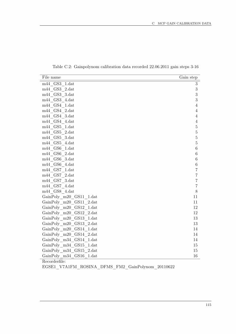
C MCP GAIN CALIBRATION DATA
Table C.2: Gainpolynom calibration data recorded 22.06.2011 gain steps 3-16
File name Gain stepm44_GS3_1.dat 3m44_GS3_2.dat 3m44_GS3_3.dat 3m44_GS3_4.dat 3m44_GS4_1.dat 4m44_GS4_2.dat 4m44_GS4_3.dat 4m44_GS4_4.dat 4m44_GS5_1.dat 5m44_GS5_2.dat 5m44_GS5_3.dat 5m44_GS5_4.dat 5m44_GS6_1.dat 6m44_GS6_2.dat 6m44_GS6_3.dat 6m44_GS6_4.dat 6m44_GS7_1.dat 7m44_GS7_2.dat 7m44_GS7_3.dat 7m44_GS7_4.dat 7m44_GS8_4.dat 8GainPoly_m20_GS11_1.dat 11GainPoly_m20_GS11_2.dat 11GainPoly_m20_GS12_1.dat 12GainPoly_m20_GS12_2.dat 12GainPoly_m20_GS13_1.dat 13GainPoly_m20_GS13_2.dat 13GainPoly_m20_GS14_1.dat 14GainPoly_m20_GS14_2.dat 14GainPoly_m34_GS14_1.dat 14GainPoly_m34_GS15_1.dat 15GainPoly_m34_GS15_2.dat 15GainPoly_m34_GS16_1.dat 16Recorderfile:EGSE1_V7A1FM_ROSINA_DFMS_FM2_GainPolynom_20110622
115

D RECORDER FILES OF THE CALIBRATION
D Recorder files of the calibration
The calibration measurements are recorded with GSEOS in the following recorderfiles anddata can be extracted thereof:
Noble Gases:EGSE1_V7AEFM_ROSINA_DFMS_FM2_Ne-sensitivity_20130405
EGSE1_V7AEFM_ROSINA_DFMS_FM2_Ar-isotopes_20130404
EGSE1_V7A9FM_ROSINA_DFMS_FM2_Kr-sensitivity_20120228EGSE1_V7A9FM_ROSINA_DFMS_FM2_Kr-sensitivity_20120229EGSE1_V7A9FM_ROSINA_DFMS_FM2_Kr-sensitivity_20120312EGSE1_V7A9FM_ROSINA_DFMS_FM2_Kr-sensitivity_20120315
EGSE1_V7A9FM_ROSINA_DFMS_FM2_Xe-sensitivity_20120710
Water:EGSE1_V7A9FM_ROSINA_DFMS_FM2_H2O_20120402EGSE1_V7A9FM_ROSINA_DFMS_FM2_H2O_20120403EGSE1_V7A9FM_ROSINA_DFMS_FM2_H2O_20120404EGSE1_V7A9FM_ROSINA_DFMS_FM2_H2O_20120405
Nitrogen:EGSE1_V7A9FM_ROSINA_DFMS_FM2_N2-sensitivity_20120423EGSE1_V7A9FM_ROSINA_DFMS_FM2_N2-sensitivity_20120424
Carbon-dioxide:EGSE1_V7A9FM_ROSINA_DFMS_FM2_CO2-sensitivity_20120503EGSE1_V7A9FM_ROSINA_DFMS_FM2_CO2-sensitivity_20120507EGSE1_V7AFFM_ROSINA_DFMS_FM2_CO2_20130416
Alkanes:EGSE1_V7A9FM_ROSINA_DFMS_FM2_CH4-sensitivity_20120607EGSE1_V7A9FM_ROSINA_DFMS_FM2_CH4-sensitivity_20120608
EGSE1_V7A9FM_ROSINA_DFMS_FM2_C2H6-sensitivity_20120711EGSE1_V7AAFM_ROSINA_DFMS_FM2_C2H6-sensitivity_20120712
EGSE1_V7A9FM_ROSINA_DFMS_FM2_C3H8-sensitivity_20120612EGSE1_V7A9FM_ROSINA_DFMS_FM2_C3H8-sensitivity_20120613EGSE1_V7AEFM_ROSINA_DFMS_FM2_C3H8-sensitivity_20130408EGSE1_V7AEFM_ROSINA_DFMS_FM2_C3H8-sensitivity_20130409
EGSE1_V7AFFM_ROSINA_DFMS_FM2_C4H10_20130411EGSE1_V7AFFM_ROSINA_DFMS_FM2_C4H10_20130412EGSE1_V7AFFM_ROSINA_DFMS_FM2_C4H10_20130415
116

D RECORDER FILES OF THE CALIBRATION
Alkene:EGSE1_V7A9FM_ROSINA_DFMS_FM2_C2H4-sensitivity_20120605EGSE1_V7A9FM_ROSINA_DFMS_FM2_C2H4-sensitivity_20120606
Gas mixtures:EGSE1_V7AFFM_ROSINA_DFMS_FM2_SW-test_20130411
EGSE1_V7A9FM_ROSINA_DFMS_FM2_ROSINA-Quiz_20120509EGSE1_V7A9FM_ROSINA_DFMS_FM2_ROSINA-Quiz_20120510
EGSE1_V7AFFM_ROSINA_DFMS_FM2_Ne-Ar-Kr-Xe_20130423
Electron energy stepping:EGSE1_V7A9FM_ROSINA_DFMS_FM2_electron-energy-stepping_20120508
117

E FRAGMENTATION PATTERN FOR MCP/LEDA AND CEM (FI
) AND POSSIBLE YIELD CORRECTIONS
E Fragmentation pattern for MCP/LEDA and CEM (fi) andpossible yield corrections
Table E.3: H2O fragmentation pattern for CEM and NIST values
Species fH2O �fH2O fH2O [%] �fH2O [%] NISTO 0.015 0.010 1.89 68.80 0.007OH 0.188 0.014 23.56 7.41 0.174H2O 0.797 0.024 100.00 3.04 0.819
Table E.4: H2O fragmentation pattern and possible yield corrections for MCP/LEDA
Species fH2O �fH2O fH2O [%] �fH2O [%] yieldO 0.021 0.011 2.61 52.75 2.017OH 0.187 0.005 23.67 2.55 1.557H2O 0.792 0.011 100.00 1.39 1.808
Table E.5: N2 fragmentation pattern for CEM and NIST values
Species fN2 �fN2 fN2 [%] �fN2 [%] NISTN 0.040 0.022 4.21 54.81 0.121N2 0.960 0.022 100.00 2.31 0.879
Table E.6: N2 fragmentation pattern and possible yield corrections for MCP/LEDA
Species fN2 �fN2 fN2 [%] �fN2 [%] yieldN 0.050 0.010 5.23 20.60 0.933N2 0.950 0.010 100.00 1.08 0.684
Table E.7: CO2 fragmentation pattern for CEM and NIST values
Species fCO2 �fCO2 fCO2 [%] �fCO2 [%] NISTC 0.012 0.003 1.47 21.03 0.067O 0.062 0.012 7.32 19.77 0.074CO++
2 0.000 0.000 0.05 89.42 0.015CO 0.078 0.011 9.24 13.47 0.075CO2 0.847 0.008 100.00 0.90 0.769
118

E FRAGMENTATION PATTERN FOR MCP/LEDA AND CEM (FI
) AND POSSIBLE YIELD CORRECTIONS
Table E.8: CO2 fragmentation pattern and possible yield corrections for MCP/LEDA
Species fCO2 �fCO2 fCO2 [%] �fCO2 [%] yieldO 0.121 0.014 15.57 11.35 1.958CO++
2 0.000 0.000 0.06 95.93 1.130CO 0.099 0.006 12.72 6.30 1.266CO2 0.779 0.016 100.00 2.08 0.920
Table E.9: CH4 fragmentation pattern for CEM and NIST values
Species fCH4 �fCH4 fCH4 [%] �fCH4 [%] NIST12C 0.004 0.001 0.56 24.92 0.01712CH 0.015 0.003 2.41 18.66 0.04812CH2 0.024 0.016 3.78 66.31 0.09112CH3 0.317 0.051 49.59 15.97 0.39712CH4 0.640 0.064 100.00 10.04 0.447
Table E.10: CH4 fragmentation pattern and possible yield corrections for MCP/LEDA
Species fCH4 �fCH4 fCH4 [%] �fCH4 [%] yield12CH 0.019 0.011 3.56 61.63 1.60512CH2 0.031 0.012 5.87 40.25 1.80312CH3 0.429 0.016 82.25 3.71 1.62312CH4 0.522 0.011 100.00 20.10 2.106
119

E FRAGMENTATION PATTERN FOR MCP/LEDA AND CEM (FI
) AND POSSIBLE YIELD CORRECTIONS
Table E.11: C2H6 fragmentation pattern for CEM and NIST values
Species fC2H6 �fC2H6 fC2H6 [%] �fC2H6 [%] NIST12C 0.001 0.000 0.18 39.13 0.00212CH 0.002 0.001 0.50 32.21 0.00512CH2 0.008 0.002 1.79 26.26 0.01412CH3 0.026 0.007 5.69 25.84 0.02012CH4 0.005 0.000 1.00 9.92 0.00012C2 0.001 0.000 0.31 8.04 0.00212C2H 0.012 0.001 2.65 7.71 0.01612C2H2 0.102 0.008 22.49 8.13 0.10712C2H3 0.135 0.009 29.75 6.93 0.15312C2H4 0.454 0.020 100.00 4.50 0.46012C2H5 0.102 0.002 22.52 2.19 0.09912C2H6 0.148 0.008 32.72 5.34 0.121
Table E.12: C2H6 fragmentation pattern and possible yield corrections for MCP/LEDA
Species fC2H6 �fC2H6 fC2H6 [%] �fC2H6 [%] yield12CH 0.003 0.001 0.59 26.30 1.47112CH2 0.012 0.007 2.32 59.32 1.52812CH3 0.043 0.023 8.16 53.62 1.34512CH4 0.000 0.005 0.00 20.10 1.83712C2 0.002 0.000 0.29 19.09 1.91812C2H 0.012 0.001 2.25 12.40 2.10012C2H2 0.114 0.024 21.59 21.02 1.90912C2H3 0.095 0.012 17.96 12.83 2.97912C2H4 0.528 0.028 100.00 5.30 1.78212C2H5 0.086 0.004 16.26 4.99 2.46812C2H6 0.106 0.017 20.10 15.76 2.911
120

E FRAGMENTATION PATTERN FOR MCP/LEDA AND CEM (FI
) AND POSSIBLE YIELD CORRECTIONS
Table E.13: C3H8 fragmentation pattern for CEM and NIST values
Species fC3H8 �fC3H8 fC3H8 [%] �fC3H8 [%] NIST12C 0.000 0.000 0.19 62.94 0.00112CH 0.001 0.000 0.60 27.12 0.00212CH2 0.004 0.001 1.82 26.49 0.00712CH3 0.025 0.003 10.66 13.08 0.02212CH4 0.013 0.001 5.82 9.66 0.00112C2 0.001 0.000 0.34 7.88 0.00012C2H 0.003 0.000 1.40 10.00 0.00212C2H2 0.027 0.002 11.83 6.30 0.02812C2H3 0.083 0.002 35.95 2.86 0.12912C2H4 0.144 0.024 62.27 16.66 0.18012C2H5 0.231 0.025 100.00 10.66 0.30713C12CH5 0.006 0.001 2.16 11.65 0.00712C3 0.000 0.000 0.08 13.37 0.00112C3H 0.005 0.000 1.96 10.60 0.00912C3H2 0.011 0.002 4.67 21.75 0.01612C3H3 0.061 0.017 26.49 27.14 0.05812C3H4 0.011 0.002 4.97 21.46 0.00912C3H5 0.060 0.011 26.15 18.83 0.04112C3H6 0.023 0.005 9.80 20.56 0.01812C3H7 0.125 0.006 54.12 4.80 0.07112C3H8 0.166 0.004 71.78 2.49 0.08413C12C2H8 0.005 0.001 2.15 13.25 0.002
121

E FRAGMENTATION PATTERN FOR MCP/LEDA AND CEM (FI
) AND POSSIBLE YIELD CORRECTIONS
Table E.14: C3H8 fragmentation pattern and possible yield corrections for MCP/LEDA
Species fC3H8 �fC3H8 fC3H8 [%] �fC3H8 [%] yield12CH 0.002 0.0004 0.82 19.74 1.6112CH2 0.007 0.0024 2.45 35.91 1.8012CH3 0.044 0.0080 15.73 18.34 1.6212CH4 0.016 0.0069 5.62 44.61 2.1112C2 0.001 0.0002 0.36 19.29 2.2012C2H 0.004 0.0011 1.54 24.97 2.0512C2H2 0.041 0.0010 14.74 2.35 1.9512C2H3 0.128 0.0217 46.37 16.89 1.9012C2H4 0.198 0.0178 71.66 8.98 2.1412C2H5 0.277 0.0260 100.00 9.38 2.3913C12CH5 0.006 0.0014 2.16 23.68 2.3912C3 0.000 0.0000 0.03 36.80 6.4612C3H 0.002 0.0004 0.84 16.35 5.4412C3H2 0.007 0.0005 2.41 7.77 4.1112C3H3 0.042 0.0138 15.32 32.62 4.1012C3H4 0.006 0.0006 2.17 10.13 4.9012C3H5 0.035 0.0020 12.73 5.80 4.4212C3H6 0.013 0.0007 4.67 5.44 4.2512C3H7 0.074 0.0065 26.62 8.84 4.8512C3H8 0.098 0.0040 35.35 4.11 4.8313C12C2H8 0.003 0.0004 1.15 14.13 4.83
122

E FRAGMENTATION PATTERN FOR MCP/LEDA AND CEM (FI
) AND POSSIBLE YIELD CORRECTIONS
Table E.15: C4H10 fragmentation pattern for CEM and NIST values
Species fC4H10 �fC4H10 fC4H10 [%] �fC4H10 [%] NIST12C 0.000 0.000 0.12 60.50 0.00012CH 0.000 0.000 0.01 127.87 0.00112CH2 0.001 0.000 0.29 20.54 0.00312CH3 0.002 0.000 0.59 16.01 0.01912CH4 0.015 0.001 4.22 6.82 0.00012C2 0.001 0.000 0.28 16.49 0.00012C2H 0.004 0.002 1.22 35.73 0.00112C2H2 0.027 0.010 7.57 35.85 0.01912C2H3 0.073 0.014 20.18 19.00 0.12412C2H4 0.081 0.026 22.45 31.63 0.10312C2H5 0.105 0.029 29.24 27.46 0.13912C2H6 0.003 0.001 0.91 29.97 0.00312C3 0.000 0.000 0.00 30.50 0.00012C3H 0.002 0.001 0.56 66.42 0.00212C3H2 0.003 0.000 0.81 14.24 0.00612C3H3 0.032 0.008 8.94 25.38 0.04412C3H4 0.006 0.001 1.73 12.64 0.00612C3H5 0.096 0.018 26.64 19.04 0.09212C3H6 0.055 0.008 15.33 13.91 0.03912C3H7 0.359 0.039 100.00 10.88 0.32112C3H8 0.018 0.003 4.89 14.85 0.01112C4H 0.000 0.000 0.14 12.49 0.00112C4H2 0.002 0.000 0.55 19.04 0.00412C4H3 0.002 0.000 0.60 13.82 0.00312C4H4 0.001 0.000 0.23 26.44 0.00112C4H5 0.003 0.001 0.74 33.89 0.00312C4H6 0.001 0.000 0.30 12.82 0.00112C4H7 0.004 0.001 1.06 19.17 0.00312C4H8 0.003 0.001 0.85 34.53 0.00312C4H9 0.010 0.002 2.70 19.71 0.00812C4H10 0.077 0.012 21.31 15.82 0.039
123

E FRAGMENTATION PATTERN FOR MCP/LEDA AND CEM (FI
) AND POSSIBLE YIELD CORRECTIONS
Table E.16: C4H10 fragmentation pattern and possible yield corrections for MCP/LEDA
Species fC4H10 �fC4H10 fC4H10 [%] �fC4H10 [%] yield12CH 0.002 0.000 0.75 13.25 1.4312CH2 0.004 0.000 1.50 6.88 1.4712CH3 0.037 0.007 12.68 18.82 1.3312CH4 0.019 0.004 6.58 21.82 1.7312C2 0.002 0.001 0.61 31.95 1.8412C2H 0.006 0.003 2.22 39.65 2.0512C2H2 0.041 0.013 13.99 30.67 1.9512C2H3 0.115 0.006 39.39 5.15 1.9012C2H4 0.120 0.026 40.98 21.87 2.1412C2H5 0.126 0.010 43.16 7.63 2.3912C2H6 0.003 0.000 0.93 15.35 3.3412C3 0.001 0.000 0.35 22.18 2.7912C3H 0.003 0.001 0.92 24.44 6.5312C3H2 0.028 0.001 9.46 4.94 3.2412C3H3 0.005 0.000 1.55 1.95 3.4612C3H4 0.083 0.014 28.50 17.15 4.2312C3H5 0.046 0.006 15.67 12.81 3.5812C3H6 0.292 0.030 100.00 10.24 3.8812C3H7 0.013 0.004 4.37 32.79 3.9312C3H8 0.000 0.000 0.12 26.57 4.3412C4H 0.000 0.000 0.09 17.80 6.0212C4H2 0.001 0.000 0.50 11.36 4.2012C4H3 0.001 0.000 0.49 3.30 4.6412C4H4 0.001 0.000 0.17 14.13 4.8612C4H5 0.002 0.000 0.53 7.72 5.0912C4H6 0.001 0.000 0.18 12.97 6.6412C4H7 0.002 0.000 0.63 18.05 6.3712C4H8 0.001 0.000 0.50 16.19 6.0912C4H9 0.005 0.001 1.65 22.25 6.3212C4H10 0.040 0.007 13.77 16.21 6.15
124

E FRAGMENTATION PATTERN FOR MCP/LEDA AND CEM (FI
) AND POSSIBLE YIELD CORRECTIONS
Table E.17: C2H4 fragmentation pattern for CEM and NIST values
Species fC2H4 �fC2H4 fC2H4 [%] �fC2H4 [%] NIST12C 0.003 0.001 0.56 21.60 0.00212CH 0.006 0.001 1.21 18.36 0.00412CH2 0.008 0.002 1.66 30.66 0.00912CH3 0.005 0.003 1.04 58.80 0.00112C2 0.013 0.002 2.90 18.53 0.01012C2H 0.058 0.016 12.47 26.96 0.03412C2H2 0.245 0.018 53.10 7.17 0.22912C2H3 0.189 0.012 40.87 6.60 0.26912C2H4 0.462 0.020 100.00 4.35 0.432
Table E.18: C2H4 fragmentation pattern and possible yield corrections for MCP/LEDA
Species fC2H4 �fC2H4 fC2H4 [%] �fC2H4 [%] yield12CH 0.011 0.006 2.42 55.48 1.15612CH2 0.009 0.003 1.92 37.43 1.80312CH3 0.006 0.004 1.33 71.58 1.62312C2 0.012 0.003 2.74 21.76 2.20112C2H 0.056 0.018 12.66 32.21 2.05212C2H2 0.253 0.020 56.97 7.90 1.94512C2H3 0.200 0.018 45.04 9.11 1.89612C2H4 0.444 0.021 100.00 4.69 2.088
125

F PRESSURE CORRECTION FACTOR FOR PRESSURE SENSOR
F Pressure correction factor for pressure sensor
The pressure measurements with the stabil ion gauge (Series 370 STABIL-ION) are speciesdependent. The pressure measurements are nominal performed for N2, while a correctionfactor is calibrated for other species. The pressure gauge is designed according to a Bayard-Albert ionization gauge with and accuracy of 6–14%. A detailed documentation can befound in [Granville-Phillips, 2007].
Table F.19: Scale factors to correct the N2 calibrated pressure readings for the Granville-Phillips SABIL-ION Vacuum measurement System [Granville-Phillips, 2007].
GAS Scale FactorN2 1.00He 5.56Ne 3.33Ar 0.775Kr 0.515Xe 0.348H2O 0.893CO2 0.704CO 0.952
126


REFERENCES
References
[A’Hearn et al., 2011] A’Hearn, M., Belton, M. J. S., Delamere, W. A., Feaga, L. M., Hamp-ton, D., Kissel, J., Klaasen, K. P., McFadden, L. A., Meech, K. J., Melosh, H. J., Schultz,P. H., Sunshine, J. M., Thomas, P. C., Veverka, J., Wellnitz, D. D., Yeomans, D. K., Besse,S., Bodewits, D., Bowling, T. J., Carcich, B. T., Collins, S. M., Farnham, T. L., Groussin,O., Hermalyn, B., Kelley, M. S., Li, J.-Y., Lindler, D. J., Lisse, C. M., McLaughlin, S. A.,Merlin, F., Protopapa, S., Richardson, J. E., and Williams, J. L. (2011). EPOXI at CometHartley 2. Science, 332:1396–1400.
[Altwegg, 2008a] Altwegg, K. (2008a). Memo DFMS FS sensitivites before launch and inflight. Technical report, University of Bern.
[Altwegg, 2008b] Altwegg, K. (2008b). Some remarks to the document: Spontaneous sen-sitivity changes of DFMS FS and Itrap/Itotal as monitor of sensitivity. Technical report,University of Bern.
[Arpigny et al., 2003] Arpigny, C., Jehin, E., Manfroid, J., Hutsemékers, D., Schulz, R.,Stüwe, J., J.-M.Zucconi, and Ilyin, I. (2003). Anomalous nitrogen isotope ratio in comets.Science, 301(5639):1522–1524.
[Balsiger et al., 2007] Balsiger, H., Altwegg, K., Bochsler, P., Eberhardt, P., Fischer, J.,Graf, S., Jäckel, A., Kopp, E., Langer, U., Mildner, M., Müller, J., Riesen, T., Rubin,M., Scherer, S., Wurz, P., Wüthrich, S., Arijs, E., Delanoye, S., Keyser, J. D., Neefs,E., Nevejans, D., Rème, H., Aoustin, C., Mazelle, C., Médale, J. L., Sauvaud, J. A.,Berthelier, J. J., Bertaux, J. L., Duvet, L., Illiano, J. M., Fuselier, S. A., Ghielmetti,A. G., Magoncelli, T., Shelley, E. G., Korth, A., Heerlein, K., Lauche, H., Livi, S., Loose,A., Mall, U., Wilken, B., Gliem, F., Fiethe, B., Gombosi, T. I., Block, B., Carignan,G. R., Fisk, L. A., Waite, J. H., Young, D. T., and Wollnik, H. (2007). ROSINA-RosettaOrbiter Spectrometer for Ion and Neutral Analysis. Space Science Review, 128:745–801.
[Balsiger et al., 1995] Balsiger, H., Altwegg, K., and Geiss, J. (1995). D/H and 18O/16Oratio in the hydronium ion and in neutral water from in situ ion measurements in cometHalley. Journal Geophysical Research, 100:5827–5834.
[Berner et al., 2002] Berner, C., Bond, P., Bourillet, L., van Casteren, J., Ellwood, J.,Kasper, M., Kletzkine, P., Schulz, R., Schwehm, G., and Warhaut, M. (2002). Rosetta:ESA’s Comet Chaser, ESA Bulletin, 112.
[Bockelée-Morvan et al., 1998] Bockelée-Morvan, D., Gautier, D., Lis, D. C., Young, K.,Keene, J., Phillips, T., Owen, T., Crovisier, J., Goldsmith, P. F., Bergin, E. A., Despois,D., and Wootten, A. (1998). Deuterated Water in the Comet C/1996 B2 (Hyakutake)and Its Implications for the Origin of Comets. Icarus, 133:147–162.
[Bockelée-Morvan et al., 2004] Bockelée-Morvan, D., Mumma, M. J., and Weaver, H. A.(2004). Comet II, chapter The Composition of Cometary Volatiles, pages 391–423. TheUniversity of Arizona Press and Tucson.
[Bockelée-Morvan et al., 2008] Bockelée-Morvan, D., N. Biver, E. J., Cochran, A. L., Wiese-meyer, H., J. Manfroid, D. H., Arpigny, C., Boissier, J., Cochran, W., Colom, P., Crovisier,J., Milutinovic, N., Moreno, R., Prochaska, J. X., Ramirez, I., Schulz, R., and Zucconi,
133

REFERENCES
J.-M. (2008). Large Excess of Heavy Nitrogen in Both Hydrogen Cyanide and Cyanogenfrom Comet 17P/Holmes . Astrophysical Journal, 679:L49–L52.
[Brown et al., 2004] Brown, M. E., Trujillo, C., and Rabinowitz, D. (2004). Discovery of acandiate inner Oort cloud planetoid. The Astrophysical Journal, 617:645–649.
[Cisela and Lauretta, 2005] Cisela, F. and Lauretta, D. (2005). Radial migration and de-hydration of phyllosilicates in the solar nebula. Earth and Planetary Science Letters,231:1–8.
[Combi et al., 2004] Combi, M. R., Harris, M., and Smyth, W. H. (2004). Comet II, chapterGas Dynamics and Kinetcs in the Cometary Coma: Theory and Observations, pages 523–550. The University of Arizona Press and Tucson.
[Controller, 2001] Controller, M.-G. (2001). Instruction Manual to Multi-Gauge ControllerPart No. L8350301.
[Crifo and Rodionov, 1997] Crifo, J. F. and Rodionov, A. V. (1997). The Dependence of theCircumnuclear Coma Structure on the Properties of the Nucleus. Icarus, 127 (2):319–353.
[de Pater and Lissauer, 2001] de Pater, I. and Lissauer, J. J. (2001). Planetary Sciences.Cambridge University Press.
[Eberhardt, 2008a] Eberhardt, P. (2008a). DFMS FS sensitivity in flight. Technical report,University of Bern.
[Eberhardt, 2008b] Eberhardt, P. (2008b). Spontaneous sensitivity changes of DFMS FSand Itrap/Itotal as monitor of sensitivity. Technical report, University of Bern.
[Eberhardt et al., 1988] Eberhardt, P., Krankowsky, D., Schulte, W., Dolder, U., Läm-merzahl, P., Berthelier, J., Woweries, J., Stubbemann, U., Hodges, R., Hoffman, J., et al.(1988). The CO and N2 abundance in comet P/Halley. Astronomy and Astrophysics,187:481–484.
[Eberhardt et al., 1995] Eberhardt, P., Reber, M., Krankowsky, D., and Hodges, R. R.(1995). The D/H and 18O/16O ratios in water from comet 1P/Halley. Astronomy andAstrophysics, 302:301–316.
[Feldman et al., 2004] Feldman, P. D., Cochran, A. L., and Combi, M. C. (2004). CometII, chapter Spectroscopic investigations of fragment species in the coma, pages 427–448.The University of Arizona Press and Tucson.
[Glassmeier et al., 2009] Glassmeier, K.-H., Boehnhardt, H., Koschny, D., Kührt, E.,Richter, I., Schulz, R., and Alexander, C. (2009). ROSETTA: ESA’s Mission to theOrigin of the Solar System, chapter The ROSETTA Mission: Flying Towards the Originof the Solar System, pages 1–20. Springer.
[Gomes et al., 2005] Gomes, R., Levison, H. F., Tsiganis, K., and Morbidelli, A. (2005).Origin of the cataclysmic Late Heavy Bombardment period of the terrestrial planets.Nature, 435:466–469.
[Granville-Phillips, 2007] Granville-Phillips (2007). Instruction Manual to Granville-PhillipsSeries 370 Stabil-Ion Vaccum Measurement Controller.
134

REFERENCES
[Handbook of Chemistry and Physics, 2012] Handbook of Chemistry and Physics (2012).Davis R. Lide and Taylor and Francis. CRC Press.
[Hartogh et al., 2011] Hartogh, P., Lis, D. C., Bockelée-Morvan, D., de Val-Borro, M., Biver,N., Küppers, M., Emprechtinger, M., Bergin, E. A., Crovasier, J., Rengel, M., Moreno,R., Szutowicz, S., and Blake, G. A. (2011). Ocean-like water in the Jupiter-family comet103P/Hartley 2. Nature, 478:218–220.
[Haser, 1957] Haser, L. (1957). Distribution d’intensite danls la tete d’une comete. Bull.Acad. R. de Belgique, Classe de Sci. 43(5):740–750.
[Hässig et al., 2013] Hässig, M., Altwegg, K., Balsiger, H., Berthelier, J., Calmonte, U.,Combic, M., Keyser, J. D., Fiethe, B., Fuselier, S., and Rubin, M. (2013). ROSINA/DFMScapabilities to measure isotopic ratios in water at comet 67P/Churyumov-Gerasimenko.Planetary and Space Science, page DOI: 10.1016/j.pss.2013.05.014.
[Irvine and Lunine, 2004] Irvine, W. M. and Lunine, J. I. (2004). Comet II, chapter TheCycle of Matter in Our Galaxy: From Clouds to Comets, pages 25–31. The University ofArizona Press and Tucson.
[Jewitt et al., 2008] Jewitt, D., Morbidelli, A., and Rauer, H. (2008). Trans-NeptunianObjects and Comets. Springer.
[Johnson and Nier, 1953] Johnson, E. and Nier, A. (1953). Angular aberrations in sectorshaped electromagnetic lenses for focusing beams of charged particles. Physicsal Review,91:10–17.
[JPL, 2013] JPL (2013). Jet Propulsion Laboratory, California Institute of Technology,Small-Body Database Browser.http : //ssd.jpl.nasa.gov/sbdb.cgi?sstr = 67P ; orb = 1; cov = 0; log = 0; cad = 0elemlast compiled 05.05.2013.
[Keller et al., 2010] Keller, H. U., Barbieri, C., Koschny, D., Lamy, P., Rickman, H., Ro-drigo, R., Sierks, H., AHearn, M. F., Angrilli, F., Barucci, M. A., Bertaux, J.-L., Cre-monese, G., Deppo, V. D., Davidsson, B., Cecco, M. D., Debei, S., Fornasier, S., Fulle,M., Groussin, O., Gutierrez, P. J., Hviid, S. F., Ip, W.-H., Jorda, L., Knollenberg, J.,Kramm, J. R., Kührt, E., Küppers, M., Lara, L.-M., Lazzarin, M., Moreno, J. L., Marzari,F., Michalik, H., Naletto, G., Sabau, L., Thomas, N., Wenzel, K.-P., Bertini, I., Besse,S., Ferri, F., Kaasalainen, M., Lowry, S., Marchi, S., Mottola, S., Sabolo, W., Schröder,S. E., Spjuth, S., and Vernazza, P. (2010). E-Type Asteroid (2867) Steins as Imaged byOSIRIS on Board Rosetta. Science, 327:190–193.
[Krasnopolsky and Mumma, 2001] Krasnopolsky, V. A. and Mumma, M. J. (2001). Sepc-troscopy of Comet Hyakutake at 80-700 Å: First detection of solar wind charge transferemission. Astrophysical Journal, 549:629–634.
[Krasnopolsky et al., 1997] Krasnopolsky, V. A., Mumma, M. J., Abott, M., Flynn, B. C.,Meech, K. J., Yeomans, D. K., Feldman, P. D., and Cosmivici, C. B. (1997). Detection ofsoft X-rays as sensitive search for noble gases in comet Hale-Bopp (C/1995 O1). Science,277:1488–1491.
135

REFERENCES
[Lamy et al., 2009] Lamy, P. L., Toth, I., Davidsson, B. J. R., Groussin, O., Gutiérez, P.,Jorda, L., Kaasalainen, M., Lowry, S. C., Schulz, R., Alexander, C., Boehnhart, H., andGlassmeier, K.-H. (2009). ROSETTA: ESA’s Mission to the Origin of the Solar System,chapter The Nucleus of Comet 67P/Churyumov-Gerasimenko, pages 21–54. Springer.
[Langer, 2003a] Langer, U. (2003a). DFMS-FM and static mode calibration. Technicalreport, University of Bern.
[Langer, 2003b] Langer, U. (2003b). DFMS-FS and static mode calibration. Technicalreport, University of Bern.
[Langer et al., 2003] Langer, U., Altwegg, K., Balsiger, H., Berthelier, J.-J., Eberhardt, P.,Fiethe, B., Fischer, J., Fuselier, S. A., Gombosi, T. I., Illiano, J.-M., Korth, A., Kopp, E.,Nevejans, D., Neefs, E., and Rubin, M. (2003). Calibration Report of DFMS-FS StaticMode Calibration. Technical report, University of Bern.
[Lara et al., 2010] Lara, L. M., Lin, Z.-Y., Rodrigo, R., and Ip, W.-H. (2010).67P/Churyumov-Gerasimenko activity evolution during its last perihelion before theRosetta encounter. Astronomy and Astrophysics, 525:1–8.
[Meier et al., 1993] Meier, R, Eberhardt, and P (1993). Velocity and ion species dependenceof the gain of microchannel plates. International Journal of Mass Spectrometry and IonProcesses, 123(1):19–27.
[Meier et al., 1998a] Meier, R., Owen, T. C., Matthews, H. E., Jewitt, D. C., Bockelée-Morvan, D., Biver, N., Crovisier, J., and Gautier, D. (1998a). A determination of theHDO/H2O Ratio in Comet C/1995 O1 (Hale-Bopp). Science, 279:842–844.
[Meier et al., 1998b] Meier, R., Owen, T. C., Matthews, H. E., Jewitt, D. C., Senay, M.,Bockelée-Morvan, D., Biver, N., Crovisier, J., and Gautier, D. (1998b). Deuterium inComet C/1995 O1 (Hale-Bopp): Detection of DCN. Science, 279:1707–1710.
[Morbidelli and Brown, 2004] Morbidelli, A. and Brown, M. E. (2004). Comet II, chapterThe Kuiper Belt and the Primordial Evolution of the Solar System, pages 175–192. TheUniversity of Arizona Press and Tucson.
[Morbidelli et al., 2005] Morbidelli, A., Levison, H. F., Tsiganis, K., and Gomes, R. (2005).Chaotic capture of Jupiter’s Trojan asteroids in the early Solar System. Nature, 435:462–465.
[Moss et al., 1995] Moss, G. P., Smith, P. A. S., Tavernier, D., et al. (1995). Glossary ofclass names of organic compounds and reactivity intermediates based on structure (IUPACRecommendations 1995). Pure and applied chemistry, 67(8):1307–1375.
[Neefs et al., 2002] Neefs, E., Illiano, J.-M., and Nevejans, D. (2002). DFMS MCP-LEDAdetector calibration in CASYMS and Flight Spare model. Technical report, Belgian In-stitute for Space Aeronomy (BIRA-IASB).
[Neefs et al., 2004] Neefs, E., Illiano, J.-M., and Nevejans, D. (2004). DFMS Detector UserManual FS version (in flight). Technical report, Belgian Institute for Space Aeronomy(BIRA-IASB).
136

REFERENCES
[Nevejans et al., 2002] Nevejans, D., Neefs, E., Kavadias, S., Merken, P., and Hoof, C. V.(2002). The leda512 integrated circuit anode array for the analog recording of massspectra. International Journal of Mass Spectrometry, 215:77–88.
[Nevejans et al., 2001] Nevejans, D., Neefs, E., Riondato, J., and Illiano, J.-M. (2001).DFMS MCP-LEDA detector calibration in CASYMS and Flight model. Technical re-port, Belgian Institute for Space Aeronomy (BIRA-IASB).
[NIST, ] NIST. NIST Chemistry WebBook, NIST Standard Reference Database Number69. http : //webbook.nist.gov/chemistry/ last compiled 05.06.2013.
[Orient and Srivastava, 1987] Orient, O. J. and Srivastava, S. K. (1987). Electron impactionisation of H2O, CO, CO2 and CH4. Journal of Physics B: Atomic and Molecular andOptical Physics, 20:3923–3936.
[Oró, 1961] Oró, J. (1961). Comets and the formation of biochemical compounds on theprimitive Earth. Nature, 290:389–390.
[Penn State University, 2013] Penn State University (2013). Departement of Astronomyand Atrophysics.http : //www2.astro.psu.edu/users/niel/astro1/slideshows/class43/slides� 43.html.
[Rao et al., 1995] Rao, M. V. V. S., Iga, I., and Srivastava, S. K. (1995). Ionization cross-sections for the production of positive ions from H2O by electron impact. Journal ofGeophysical Research, 100:421–426.
[Rice University, 2013] Rice University (2013). Physics and Astrononmy department andAtomic and Molecular Collision Group.http : //www.ruf.rice.edu/ ⇠ atmol/electron_data.html last compiled 05.05.2013.
[Riesen, 2007] Riesen, T. (2007). Calibration of the ROSINA DFMS in a static and dy-namic environment. PhD thesis, University of Bern, Philosophisch-naturwissenschaftlicheFakultät.
[Schläppi, 2011] Schläppi, B. (2011). Characterization of the ROSINA Double FocusingMass Spectrometer. PhD thesis, University of Bern, Philosophisch-naturwissenschaftlicheFakultät.
[Schläppi et al., 2010] Schläppi, B., Altwegg, K., Balsiger, H., Hässig, M., Jäckel, A., Wurz,P., Fiethe, B., Rubin, M., Fuselier, S. A., Berthelier, J. J., Keyser, J. D., Réme, H.,and Mall, U. (2010). Influence of spacecraft outgassing on the exploration of tenuousatmospheres with in situ mass spectrometry. Journal of Geophysical Research, 115:12313.
[Schulz et al., 2009] Schulz, R., Alexander, C., Boehnhart, H., and Glassmeier, K.-H., edi-tors (2009). ROSETTA: ESA’s Mission to the Origin of the Solar System. Springer.
[Schulz et al., 2012] Schulz, R., Sierks, H., Küppers, M., and Accomazzo, A. (2012). Rosettafly-by at asteroid (21) Lutetia: An overview. Planetary and Space Science, 66(1):2–8.
[Schwehm and Schulz, 1999] Schwehm, G. and Schulz, R. (1999). ROSETTA goes to Wirta-nen. Space Science Review, 90:313–319.
137

REFERENCES
[Svitil and Foley, 2004] Svitil, K. A. and Foley, D. (2004). Beyond pluto. Discover, Novem-ber 2004.
[Tenishev, 2011] Tenishev, V. (2011). Numerical Simulation of Dust in a CometaryComa: Application to Comet 67P/Churyumov-Gerasimenko. The Astrophysical Jour-nal, 732:104:17.
[Tenishev et al., 2008] Tenishev, V., Combi, M. C., and Davidsson, B. (2008). A globalkinetic model for cometary comae: The evolution of the coma of the Rosetta target cometChuryumov-Gerasimenko throughout the mission. Astrophysical Journal, 685:659–677.
[Tsiganis et al., 2005] Tsiganis, K., Gomes, R., Morbidelli, A., and Levison, H. F. (2005).Origin of the orbital architecture of the giant planets of the Solar System. Nature, 435:459–461.
[University of Michigan, 2013] University of Michigan (2013). ICES - Inner Coma Environ-ment Simulator. http : //ices.engin.umich.edu/index.php last compiled 05.05.2013.
[Weaver et al., 2008] Weaver, H. A., A’Hearn, M. F., Arpigny, C., Combi, M. R., Feldman,P. D., Tozzi, G.-P., Russo, N. D., and Festou, M. C. (2008). Atomic Deuterium Emissionand the D/H ratio in Comets. Asteroids and Comets and Meteors, 1405:8216.
[Westermann, 2000] Westermann, C. B. (2000). A Novel Calibration System for the Sim-ulation of Cometary Atmospheres. PhD thesis, University of Bern, Philosophisch-naturwissenschaftliche Fakultät.
[Westermann et al., 2001] Westermann, C. B., Luithard, W., Kopp, E., Koch, T., Linger,R., Hofstetter, H., Fischer, J., Altwegg, K., and Balsiger, H. (2001). A high precisioncalibration system for the simulation of cometary gas environments. Measurement Scienceand Technology, 12:1594–1603.
[Wüthrich, 2007] Wüthrich, S. (2007). Characterization of the ROSINA DFMS In-strument by Numerical Modelling. PhD thesis, University of Bern, Philosophisch-naturwissenschaftliche Fakultät.
[Zahnd, 2002] Zahnd, B. (2002). DFMS FM2 Recertification Thermal-Vacuum Test. Tech-nical report, University of Bern.
[Ziurys et al., 1999] Ziurys, L. M., Savage, C., Brewster, M. A., Apponi, A. J., Pesch, T. C.,and Wyckoff, S. (1999). Cyabice chemistry in comet Hale-Bopp (C/1995 O1). Astrophysic-sal Journal Letters, 527:L67–L71.
138

REFERENCES
Acknowledgments
I would like to thank my advisor, Prof. Dr. Kathrin Altwegg for the unique opportunity to writemy PhD thesis on such an interesting project as the ROSINA DFMS. I appreciate the many fruit-ful discussions and the infinite patience as well as the permanent support at any occasions. I alsoappreciate all the possibilities to attend many meetings and conferences to present our work andenlarge my horizon at countless occasions.
Special thanks go to Prof. Dr. Cécile Engrand from the University of Paris for refereeing this work.
The operation and maintenance of DFMS requires technical assistance from many individuals fromthe whole physics institute. I owe many thanks to:
- Harry Mischler and the mechanics for helping hands when ever needed.
- Adrian Etter for the support with CASYMIR and CASYMS and helping hands when everneeded.
- Jürg Jost for the repair of the RDP electronics and the GCU.
Furthermore I owe many thanks to:
- Dr. Bernhard Schläppi for the collaboration with DFMS, for the many fruitful discussionsand for staying relaxed when DFMS shows unexpected anomalies.
- Dr. Annette Jäckel for all the fruitful discussions, for the support to find references and beingthere when ever a helping hand or a listening ear is needed.
- Dr. Martin Rubin for all the fruitful discussions, for reading through my thesis and your neverending patience.
- Dr. Léna Le Roy for taking care of DFMS, for the collaboration and for reading through mythesis.
- Dr. André Bieler for the collaboration and for reading through my thesis.
- Ursina Calmonte, Chia-You (Helen) Tzou, Sébastien Gasc and Thierry Sémon for the collab-oration.
- Prof. Ernest Kopp for all the fruitful discussions and your help to find pictures.
- Prof. Hand Balsiger as honorary PI and many fruitful discussions.
- Prof. Peter Wurz for the collaboration and the fruitful discussions.
- Brain Magee for reading trough parts of my thesis.
- The ROSINA team members for the collaboration, for advices in many situations, for supportand proofreading of drafts.
- Many others for help in administrative and technical matters or being nice roommates.
Finally, I would like to thank my parents and my brother for all their support. Special thanks toBeat who experienced the struggles and the time consuming of such a work first hand. Thank youfor bringing me back to Earth again when things tend to get out of hand and make me smile again.
This work was funded by the Swiss National Science Foundation, the Prodex Program of the Euro-pean Space Agency, and the Kanton of Bern.
139


! " # $ % " & '(()
!"#$%%&'()*&+,&'-%*&+&./0&12
34#"567(84#"9 �*$$����)#%�����#�� �
:4)(;<"=8>##"(9 ����������
/)>?;"8!48!9 ��)$��
@4AB"=7(&&&&! :4%)"(&&&&! &&&&&&&&&&&C;%%"()4);78&&&&!
D;)"=&?"(&'(-";)9 �� $�%�'�%)� � �� �#���� %�%�! � �����#�%�! � !�� %��� �������!&����
!�&$� ����$$��"��%#!��%�#
0";)"(E8&?"(&'(-";)9 �#!���#�� �%�#� ���%(����
EAB&"(<=$("&B;"(#;)F &?4%%& ;AB&?;"%"&'(-";) &%"=-%)$8?;!&G"(H4%%)&>8?&<";8"&48?"("8&4=%&?;"&
48!"!"-"8"8&I>"=="8&-"8>)J)&B4-"*&'=="&/)"=="8F&?;"&KL()=;AB&7?"(&%;88!"#$%%&4>%&I>"=="8&
"8)87##"8&K>(?"8F&B4-"&;AB&4=%&%7=AB"&!"<"88J";AB8")*&:;(&;%)&-"<488)F&?4%%&48?"(8H4==%&
?"(&/"84)&!"#$%%&'();<"=&MN&'-%4)J&O&@>AB%)4-"��&?"%&P"%")J)"%&G7#&2*&/"Q)"#-"(&ORRN&
S-"(&?;"&T8;G"(%;)$)&J>#&U8)J>!&?"%&4>H&P(>8?&?;"%"(&'(-";)&G"(=;"B"8"8&D;)"=%&-"("AB);!)&;%)*
******************************************************************
V()5C4)>#
*************************************************************
T8)"(%AB(;H)
�


REFERENCES
Curriculum Vitae
Personal Data
Name: HässigFirst Name: Myrtha MarianneDate of birth: 13.07.1984Adress: Dorfstrasse 2, 3655 Sigriswil, Switzerland
Education
1991-1997 Primary school in Sigriswil1997-1999 Secondary school in Sigriswil1999-2003 Grammar school in Thun-Schadau2003 Matura at Gymnasium Thun-Schadau
main focus physics and applied mathematics
Academic record
2003-2008 Studies at the University of Bern in experimental physics,mathematics and philosophies (science history and science theory)
2007-2008 Master’s thesis in physics at the Institute of Applied Physics,University of Bern, Division of Laser Physics,entitled: "Optical fibers with a conductive core",Supervisor: Prof. Dr. Willy Lüthy
2008-2010 Diploma of teaching physics at grammar school of PH Bern2009-2013 PhD thesis in experimental physics at the physics institute,
University of Bern, Division of Space Research and Planetary Science,entitled: "Sensitivity and fragmentation calibration
of the ROSINA Double Focusing Mass Spectrometer",Supervisor: Prof. Dr. Kathrin Altwegg
Professional Training
2002-2006 Internship at the engineering departmentof Frutiger AG (construction firm) in Thun
2008-2012 Teaching physics at Gymnasium und Fachmittelschule Thun-Seefeld2009-2013 Teaching assistant at University of Bern of physics exercises and
laboratory classes for students of medicine and other branches
143