Sensitivity analysis of TOPSIS method in water quality assessment II: sensitivity to the index input...

1 23

Environmental Monitoring andAssessmentAn International Journal Devoted toProgress in the Use of Monitoring Datain Assessing Environmental Risks toMan and the Environment ISSN 0167-6369Volume 185Number 3 Environ Monit Assess (2013)185:2463-2474DOI 10.1007/s10661-012-2724-8

Sensitivity analysis of TOPSIS method inwater quality assessment II: sensitivity tothe index input data

Peiyue Li, Jianhua Wu, Hui Qian & JieChen

1 23

Your article is protected by copyright and

all rights are held exclusively by Springer

Science+Business Media B.V.. This e-offprint

is for personal use only and shall not be self-

archived in electronic repositories. If you

wish to self-archive your work, please use the

accepted author’s version for posting to your

own website or your institution’s repository.

You may further deposit the accepted author’s

version on a funder’s repository at a funder’s

request, provided it is not made publicly

available until 12 months after publication.

Sensitivity analysis of TOPSIS method in water qualityassessment II: sensitivity to the index input data

Peiyue Li & Jianhua Wu & Hui Qian & Jie Chen

Received: 14 November 2011 /Accepted: 11 June 2012 /Published online: 26 July 2012# Springer Science+Business Media B.V. 2012

Abstract This is the second part of the study onsensitivity analysis of the technique for order preferenceby similarity to ideal solution (TOPSIS) method in waterquality assessment. In the present study, the sensitivityof the TOPSIS method to the index input data wasinvestigated. The sensitivity was first theoretically ana-lyzed under two major assumptions. One assumptionwas that one index or more of the samples were per-turbed with the same ratio while other indices keptunchanged. The other one was that all indices of a givensample were changed simultaneously with the sameratio, while the indices of other samples wereunchanged. Furthermore, a case study under assumption2 was also carried out in this paper. When the sameindices of different water samples are changed simulta-neously with the same variation ratio, the final waterquality assessment results will not be influenced at all.When the input data of all indices of a given sample areperturbed with the same variation ratio, the assessmentvalues of all samples will be influenced theoretically.However, the case study shows that only the perturbedsample is sensitive to the variation, and a simple linearequation representing the relation between the closenesscoefficient (CC) values of the perturbed sample andvariation ratios can be derived under the assumption 2.

This linear equation can be used for determining thesample orders under various variation ratios.

Keywords Sensitivity analysis .Water quality .

TOPSIS . Uncertainty .Multiple-criteria decisionmaking . Assessment method . Input data

Introduction

Sensitivity analysis is regarded as an indispensable stepfor the analysis of various multiple-criteria decision-making problems. Decision makers are always eagerto know whether their decisions are sensitive to thechanging environment, and they are also interested indetermining the most important factors which mostlyaffect their decisions. Generally speaking, the aim ofsensitivity analysis is to quantify the effects of parametervariations on calculated results (Cacuci 2003). Manyterms, such as influence, importance, ranking by impor-tance and dominance, are all related to sensitivity anal-ysis. Typically, sensitivity analysis can be performedeither comprehensively or just partially, according towhich sensitivity analysis can be classified as globalanalysis and local analysis (Cacuci et al. 2005). Themethods for sensitivity analysis include deterministicmethods and statistical methods (Cacuci and Ionescu-Bujor 2004; Ionescu-Bujor and Cacuci 2004; Cacuci etal. 2005). For different users and aims, the methods usedfor sensitivity analysis are different and thereforewith different complexity (Cacuci 2003). However,

Environ Monit Assess (2013) 185:2463–2474DOI 10.1007/s10661-012-2724-8

P. Li (*) : J. Wu :H. Qian : J. ChenSchool of Environmental Science and Engineering,Chang’an University,No.126 Yanta Road,Xi’an 710054, Shaanxi, People’s Republic of Chinae-mail: [email protected]

Author's personal copy

the most common method used practically is basedon the perturbation theory which gives the inputparameter a small perturbation, and then recalculatesthe results to see how the result will be influenced.This probably is the most traditional and easiestway for quantifying the sensitivity.

So far, there have already been several studies onthe sensitivity analysis of methods for water relatedstudies. Xu and Xue (1994) introduced the concept ofsensitivity of Comprehensive Index of EnvironmentalQuality and derived the mathematical expressions ofthe sensitivity. Yuan et al. (1998), based on the studyby Xu and Xue (1994), redefined the concept of sen-sitivity of the index methods in environmental qualityassessment, and they also performed sensitivity anal-ysis of several commonly used index methods.Manache and Melching (2004) investigated the effectof parameter uncertainties on prediction model forthe Dender River in Belgium by Latin hypercubesampling technique in combination with regressionand correlation analyses. Rickwood and Carr (2009)carried out a preliminary sensitivity analysis andverification of a composite index against real waterquality data. Nakane and Haidary (2010) performedsensitivity analysis of two water quality predictionmodels based on Monte Carlo method. Aimed atimproving the precision and decreasing the uncer-tainty in forecasting hydrological time series, Yanget al. (2009) proposed a chaotic Bayesian methodbased on multiple-criteria decision making. Theyalso proposed an ideal interval method of multi-objective decision-making (Yang et al. 2004) and aNonlinear Optimization Set Pair Analysis Model(Yang et al. 2011) for Assessing Water ResourceRenewability. These existing works provide strongtheoretic basis for the present study.

The technique for order preference by similarity toideal solution (TOPSIS) method is one of the mostpopular multiple-criteria decision-making methods. Ithas been incorporated with fuzzy theory and manyother theories, and has been widely used in variousfields (Hyde et al. 2005; Sadi-Nezhad and Damghani2010; Awasthi et al. 2011; Afshar et al. 2011; Li et al.2011a, b). However, comprehensive studies onTOPSIS-related sensitivity analysis are rare, therefore,the study aims to (1) assess the sensitivity of theTOPSIS method to the variations of index input dataand (2) examine the feasibility and reliability of theTOPSIS method in water quality assessment.

Summary of TOPSIS

TOPSIS was first proposed by Hwang and Yoon(1981) for the purpose of solving multiple attributedecision-making problems with no articulation ofpreference information. The specific steps of waterquality assessment using TOPSIS have been discussedin detail by Li et al. (2011a, b). Generally, to perform awater quality assessment using TOPSIS, six stepsmust be followed. The steps are summarized here,and for a detailed introduction the reader can refer tothe literatures published by Li et al. (2011a, b).

& Step 1: constructing the initial decision matrix Caccording to the observed water quality data

& Step 2: normalizing the initial decision matrix toeliminate the effects of complex relations. Thenormalized value rij is calculated as

rij ¼cij=

Pmi¼1

c2ij

� �12

efficiency type

�cij=Pmi¼1

c2ij

� �12

cost type

8>>><>>>:

ð1Þ

& Step 3: determining the weight of each index wj

and calculating the weighted normalized decisionmatrix F. The weighted normalized value fij iscalculated as

fij ¼ rij � wj ð2Þ& Step 4: determining the positive and negative ideal

reference points

G ¼ f þ1 ; f þ2 . . . f þn� �

B ¼ f �1 ; f �2 . . . f �n� ��

ð3Þ

f þj ¼ max f1j; f2j . . . fmj� �

f �j ¼ min f1j; f2j . . . fmj� � j ¼ 1; 2; . . . nð Þ

(ð4Þ

Where, G and B are respectively the positive idealreference point and the negative ideal reference point.& Step 5: calculating the distances to the positive and

negative ideal referencepointsusingEuclideandistance

dþ ¼ffiffiffiffiffiffiffiffiffiffiffiffiffiffiffiffiffiffiffiffiffiffiffiffiffiffiffiffiffiffiffiffiPnj¼1

fij � fij�

G

h i2s

d� ¼ffiffiffiffiffiffiffiffiffiffiffiffiffiffiffiffiffiffiffiffiffiffiffiffiffiffiffiffiffiffiffiPnj¼1

fij � fij�

B

�2s8>>>><>>>>:

ð5Þ

2464 Environ Monit Assess (2013) 185:2463–2474


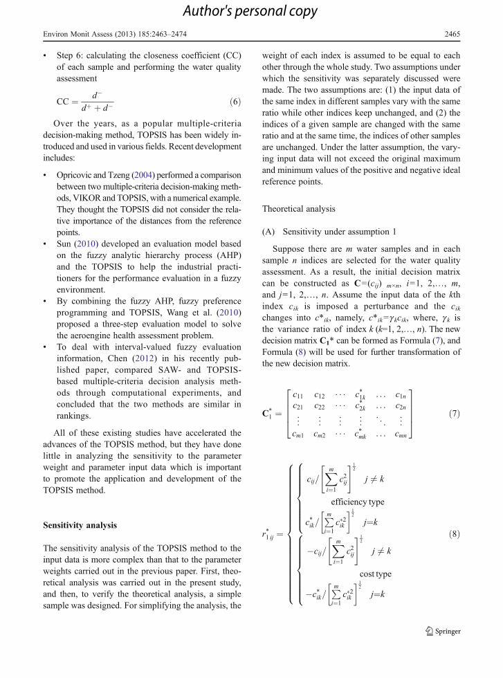
& Step 6: calculating the closeness coefficient (CC)of each sample and performing the water qualityassessment

CC ¼ d�

dþ þ d�ð6Þ

Over the years, as a popular multiple-criteriadecision-making method, TOPSIS has been widely in-troduced and used in various fields. Recent developmentincludes:

& Opricovic and Tzeng (2004) performed a comparisonbetween two multiple-criteria decision-making meth-ods, VIKOR and TOPSIS, with a numerical example.They thought the TOPSIS did not consider the rela-tive importance of the distances from the referencepoints.

& Sun (2010) developed an evaluation model basedon the fuzzy analytic hierarchy process (AHP)and the TOPSIS to help the industrial practi-tioners for the performance evaluation in a fuzzyenvironment.

& By combining the fuzzy AHP, fuzzy preferenceprogramming and TOPSIS, Wang et al. (2010)proposed a three-step evaluation model to solvethe aeroengine health assessment problem.

& To deal with interval-valued fuzzy evaluationinformation, Chen (2012) in his recently pub-lished paper, compared SAW- and TOPSIS-based multiple-criteria decision analysis meth-ods through computational experiments, andconcluded that the two methods are similar inrankings.

All of these existing studies have accelerated theadvances of the TOPSIS method, but they have donelittle in analyzing the sensitivity to the parameterweight and parameter input data which is importantto promote the application and development of theTOPSIS method.

Sensitivity analysis

The sensitivity analysis of the TOPSIS method to theinput data is more complex than that to the parameterweights carried out in the previous paper. First, theo-retical analysis was carried out in the present study,and then, to verify the theoretical analysis, a simplesample was designed. For simplifying the analysis, the

weight of each index is assumed to be equal to eachother through the whole study. Two assumptions underwhich the sensitivity was separately discussed weremade. The two assumptions are: (1) the input data ofthe same index in different samples vary with the sameratio while other indices keep unchanged, and (2) theindices of a given sample are changed with the sameratio and at the same time, the indices of other samplesare unchanged. Under the latter assumption, the vary-ing input data will not exceed the original maximumand minimum values of the positive and negative idealreference points.

Theoretical analysis

(A) Sensitivity under assumption 1

Suppose there are m water samples and in eachsample n indices are selected for the water qualityassessment. As a result, the initial decision matrixcan be constructed as C0(cij) m×n, i01, 2,…, m,and j01, 2,…, n. Assume the input data of the kthindex cik is imposed a perturbance and the cikchanges into c*ik, namely, c*ik0gkcik, where, gk isthe variance ratio of index k (k=1, 2,…, n). The newdecision matrix C1* can be formed as Formula (7), andFormula (8) will be used for further transformation ofthe new decision matrix.

C*1 ¼

c11 c12 � � � c*1k . . . c1nc21 c22 � � � c*2k . . . c2n... ..

. ... ..

. . .. ..

.

cm1 cm2 � � � c*mk . . . cmn

26664

37775 ð7Þ

r*1 ij ¼

cij=Xmi¼1

c2ij

" #12

j 6¼ k

efficiency type

c*ik=Pmi¼1

c�2ik

� �12

j¼k

8>>>>>>><>>>>>>>:

�cij=Xmi¼1

c2ij

" #12

j 6¼ k

cost type

�c*ik=Pmi¼1

c�2ik

� �12

j¼k

8>>>>>>><>>>>>>>:

8>>>>>>>>>>>>>>>>>>>><>>>>>>>>>>>>>>>>>>>>:

ð8Þ

Environ Monit Assess (2013) 185:2463–2474 2465


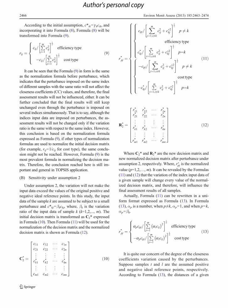
According to the initial assumption, c*ik0gkcik, andincorporating it into Formula (8), Formula (8) will betransformed into Formula (9).

rij ¼cij=

Pmi¼1

c2ij

� �12

efficiency type

�cij=Pmi¼1

c2ij

� �12

cost type

8>>><>>>:

ð9Þ

It can be seen that the Formula (9) in form is the sameas the normalization formula before perturbance, whichindicates that the perturbance imposed on the same indexof different samples with the same ratio will not affect thecloseness coefficients (CC) values, and therefore, the finalassessment results will not be influenced, either. It can befurther concluded that the final results will still keepunchanged even through the perturbance is imposed onseveral indices simultaneously. That is to say, although theindices input data are imposed on perturbances, the as-sessment results will not be changed only if the variationratio is the same with respect to the same index. However,this conclusion is based on the normalization formulaexpressed as Formula (9), if other types of normalizationformulas are used to normalize the initial decision matrix(for example, rij01/cij for cost type), the same conclu-sion might not be reached. However, Formula (9) is themost prevalent formula in normalizing the decision ma-trix. Therefore, the conclusion reached here is still im-portant and general in TOPSIS application.

(B) Sensitivity under assumption 2

Under assumption 2, the variation will not make theinput data exceed the values of the original positive andnegative ideal reference points. In this study, the inputdata of the sample k are assumed to be subject to a smallperturbance and c*kj0βkckj, where, βk is the variationratio of the input data of sample k (k=1,2,..., m). Theinitial decision matrix is transformed as C2* expressedin Formula (10). Then Formula (11) will be used for thenormalization of the decision matrix and the normalizeddecision matrix is shown as Formula (12).

C*2 ¼

c11 c12 � � � c1nc21 c22 � � � c2n... ..

. ... ..

.

c*k1 c*k2 � � � c*kn... ..

. ... ..

.

cm1 cm2 � � � cmn

2666666664

3777777775

ð10Þ

r*pj ¼

cpj=Xm

i¼1;i 6¼k

c2ij þ c�2kj

" #12

p 6¼ k

efficiency type

c*kj=Pm

i¼1;i 6¼kc2ij þ c�2kj

" #12

p¼k

8>>>>>>>><>>>>>>>>:

�cpj=Xm

i¼1;i6¼k

c2ij þ c�2kj

" #12

p 6¼ k

cost type

�c*kj=Pm

i¼1;i6¼kc2ij þ c�2kj

" #12

p¼k

8>>>>>>>><>>>>>>>>:

8>>>>>>>>>>>>>>>>>>>>>>><>>>>>>>>>>>>>>>>>>>>>>>:

ð11Þ

R*2 ¼

r*11 r*12 � � � r*1nr*21 r*22 � � � r*2n... ..

. ... ..

.

r*k1 r*k2 � � � r*kn... ..

. ... ..

.

r*m1 r*m2 � � � r*mn

2666666664

3777777775

ð12Þ

Where C2* and R2* are the new decision matrix andnew normalized decision matrix after perturbance underassumption 2, respectively. Where, r�pj is the normalized

value (p=1,2,…, m). It can be revealed by the Formulas(11) and (12) that the variation of the index input data ofa given sample will change every value of the normal-ized decision matrix, and therefore, will influence thefinal assessment results of all samples.

Actually, Formula (11) can be rewritten in a uni-form format expressed as Formula (13). In Formula(13), αp is a number, when p≠k, αp01, and when p0k,αp0βk.

r*pj ¼apcpj=

Pmi¼1

aicij� 2� �1

2

efficiency type

�apcpj=Pmi¼1

aicij� 2� �1

2

cost type

8>>><>>>:

ð13Þ

It is quite our concern of the degree of the closenesscoefficients variation caused by the perturbances.Suppose samples t and l are the assumed positiveand negative ideal reference points, respectively.According to Formula (13), the distances of a given



sample (for example, sample p) to the positive and nega-tive ideal reference points are calculated respectively as:

d�þp ¼

ffiffiffiffiffiffiffiffiffiffiffiffiffiffiffiffiffiffiffiffiffiffiffiffiffiffiffiffiffiffiffiffiffiffiffiffiffiffiffiffiffiffiffiffiffiffiffiffiffiffiffiffiffiffiffiffiffiffiffiffiffiffiffiffiffiffiffiffiffiffiPnj¼1

wjapcpjPmi¼1

ðaicijÞ2� 1

2� wjatctjPm

i¼1

ðaicijÞ2� 1

2

26664

377752

vuuuuuut

d��p ¼

ffiffiffiffiffiffiffiffiffiffiffiffiffiffiffiffiffiffiffiffiffiffiffiffiffiffiffiffiffiffiffiffiffiffiffiffiffiffiffiffiffiffiffiffiffiffiffiffiffiffiffiffiffiffiffiffiffiffiffiffiffiffiffiffiffiffiffiffiffiffiPnj¼1

wjapcpjPmi¼1

ðaicijÞ2� 1

2� wjalcljPm

i¼1

ðaicijÞ2� 1

2

26664

377752

vuuuuuut

8>>>>>>>>>>>>>><>>>>>>>>>>>>>>:

ð14Þ

Thus, the closeness coefficient of sample p (CC*p)after perturbance can be calculated according toFormula (15).

CC*p ¼ d��p

d�þp þd��p

ffiffiffiffiffiffiffiffiffiffiffiffiffiffiffiffiffiffiffiffiffiffiffiffiffiffiffiffiffiffiffiffiffiffiffiffiffiffiffiffiffiffiffiffiffiffiffiffiffiffiffiffiffiffiffiffiffiffiffiffiffiffiPnj¼1

wjapcpjPmi¼1

ðaicijÞ2

� 12� wjal cljPm

i¼1

ðaicijÞ2

� 12

26664

37775

2vuuuuuut

ffiffiffiffiffiffiffiffiffiffiffiffiffiffiffiffiffiffiffiffiffiffiffiffiffiffiffiffiffiffiffiffiffiffiffiffiffiffiffiffiffiffiffiffiffiffiffiffiffiffiffiffiffiffiffiffiffiffiffiffiffiffiPnj¼1

wjapcpjPmi¼1

ðaicijÞ2

� 12� wjat ctjPm

i¼1

ðai cijÞ2

� 12

26664

37775

2vuuuuuut þ

ffiffiffiffiffiffiffiffiffiffiffiffiffiffiffiffiffiffiffiffiffiffiffiffiffiffiffiffiffiffiffiffiffiffiffiffiffiffiffiffiffiffiffiffiffiffiffiffiffiffiffiffiffiffiffiffiffiffiffiffiPnj¼1

wjapcpjPmi¼1

ðai cijÞ2

� 12� wjal cljPm

i¼1

ðaicijÞ2

� 12

26664

37775

vuuuuuut

2 ð15Þ

It is assumed that the weights of different indicesare equal to each other, and therefore Formula (15) canbe simplified as:

CC*p ¼

ffiffiffiffiffiffiffiffiffiffiffiffiffiffiffiffiffiffiffiffiffiffiffiffiffiffiffiPnj¼1

apcpj�alcljð Þ2Pmi¼1

aicijð Þ2vuut


apcpj�at ctjð Þ2Pmi¼1

aicijð Þ2vuut þ


apcpj�al cljð Þ2Pmi¼1

aicijð Þ2vuut

ð16Þ

For convenience, Formula (16) can be rewritten asFormula (17):

1

CC*p

¼


apcpj�atctjð Þ2Pmi¼1

aicijð Þ2vuut


apcpj�alcljð Þ2Pmi¼1

aicijð Þ2vuut

þ 1 ¼

ffiffiffiffiffiffiffiffiffiffiffiffiffiffiffiffiffiffiffiffiffiffiffiffiffiffiffiffiffiffiffiffiffiffiffiffiffiffiffiffiffiffiffiffiPnj¼1

apcpj�at ctjð Þ2Pmi¼1;i 6¼k

ðcijÞ2�

þ bk ckjð Þ2

vuuutffiffiffiffiffiffiffiffiffiffiffiffiffiffiffiffiffiffiffiffiffiffiffiffiffiffiffiffiffiffiffiffiffiffiffiffiffiffiffiffiffiffiffiffiffiPnj¼1

apcpj�al cljð Þ2Pmi¼1;i6¼k

cijð Þ2�

þ bk ckjð Þ2

vuuutþ 1

ð17Þ

Formula (17) is actually a function of initial matrix Cand βk, hence, it can be expressed as 1

CC*p¼ f C; bkð Þ þ 1.

For a given initial matrix C, the function f(C, βk) changes

into f(βk), and all we have to do is to identify the relation-ship between f(βk) and βk. Namely:

f bkð Þ ¼

ffiffiffiffiffiffiffiffiffiffiffiffiffiffiffiffiffiffiffiffiffiffiffiffiffiffiffiffiffiffiffiffiffiffiffiffiffiffiffiffiffiffiffiffiPnj¼1

apcpj�at ctjð Þ2Pmi¼1;i6¼k

ðcijÞ2�

þ bk ckjð Þ2

vuuutffiffiffiffiffiffiffiffiffiffiffiffiffiffiffiffiffiffiffiffiffiffiffiffiffiffiffiffiffiffiffiffiffiffiffiffiffiffiffiffiffiffiffiffiPnj¼1

apcpj�al cljð Þ2Pmi¼1;i6¼k

ðcijÞ2�

þ bk ckjð Þ2

vuuutð18Þ

For a given C, four different forms of f(βk) existaccording to which sample is imposed a perturbance.In this study, sample k was assumed to be the per-turbed sample, and then as a result:

(a) Case 1: p≠k, t≠k, and l≠kUnder this circumstance, αp0αt0αl01, and

Formula (18) can be rewritten as

f ðbkÞ ¼

ffiffiffiffiffiffiffiffiffiffiffiffiffiffiffiffiffiffiffiffiffiffiffiffiffiffiffiffiffiffiffiffiffiffiffiffiffiffiffiffiffiffiffiffiffiPnj¼1

cpj�ctjð Þ2Pmi¼1;i 6¼k

cijð Þ2�

þ bk ckjð Þ2


cpj�cljð Þ2Pmi¼1;i 6¼k

cijð Þ2�

þ bk ckjð Þ2

vuuutð19Þ



(b) Case 2: p0k, but t≠k and l≠kIn this case, αp0βk, αt0αl01, and Formula

(18) can be rewritten as

f bkð Þ ¼


bk ckj�ctjð Þ2Pmi¼1;i 6¼k

cijð Þ2�

þ bk ckjð Þ2


bk ckj�cljð Þ2Pmi¼1;i 6¼k

cijð Þ2�

þ bk ckjð Þ2

vuuutð20Þ

(c) Case 4: p≠k and l≠k, but t0kUnder this condition, αl0βk, αp0αt01, and

Formula (18) can be rewritten as

f bkð Þ ¼


cpj�ctjð Þ2Pmi¼1;i 6¼k

cijð Þ2�

þ bk ckjð Þ2


cpj�bk ckjð Þ2Pmi¼1;i 6¼k

cijð Þ2�

þ bk ckjð Þ2

vuuutð21Þ

d) Case 3: p≠k and t≠k, but l0kIn this case, αt0βk, αp0αl01, and Formula

(18) can be rewritten as

f bkð Þ ¼


cpj�bk ckjð Þ2Pmi¼1;i 6¼k

cijð Þ2�

þ bk ckjð Þ2


cpj�cljð Þ2Pmi¼1;i 6¼k

cijð Þ2�

þ bk ckjð Þ2

vuuutð22Þ

It can be seen from the above derivation that whenthe perturbed samples are different, the influencesare different. For a given initial matrix C, thevariations of CC values are solely dependent on

the variation ratio β. However, the derivation isonly for theoretical analysis, and it is difficult toquantify the influences directly from the abovederived functions.

Case study

The above theoretical analysis indicates that the finalCC values under assumption 1 will not be influencedby the perturbances only if the variation ratios of theindices are the same. Therefore, in the case study, thecase under assumption 1 is not discussed, and ourattention will be focused solely on the discussionunder assumption 2.

(A) Initial input data

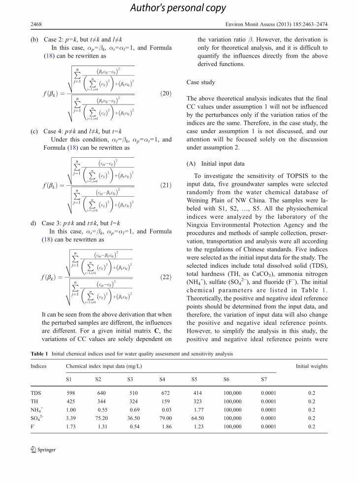
To investigate the sensitivity of TOPSIS to theinput data, five groundwater samples were selectedrandomly from the water chemical database ofWeining Plain of NW China. The samples were la-beled with S1, S2, …, S5. All the physiochemicalindices were analyzed by the laboratory of theNingxia Environmental Protection Agency and theprocedures and methods of sample collection, preser-vation, transportation and analysis were all accordingto the regulations of Chinese standards. Five indiceswere selected as the initial input data for the study. Theselected indices include total dissolved solid (TDS),total hardness (TH, as CaCO3), ammonia nitrogen(NH4

+), sulfate (SO42−), and fluoride (F−). The initial

chemical parameters are l is ted in Table 1.Theoretically, the positive and negative ideal referencepoints should be determined from the input data, andtherefore, the variation of input data will also changethe positive and negative ideal reference points.However, to simplify the analysis in this study, thepositive and negative ideal reference points were

Table 1 Initial chemical indices used for water quality assessment and sensitivity analysis

Indices Chemical index input data (mg/L) Initial weights

S1 S2 S3 S4 S5 S6 S7

TDS 598 640 510 672 414 100,000 0.0001 0.2

TH 425 344 324 159 323 100,000 0.0001 0.2

NH4+ 1.00 0.55 0.69 0.03 1.77 100,000 0.0001 0.2

SO42- 3.39 75.20 36.50 79.00 64.50 100,000 0.0001 0.2

F- 1.73 1.31 0.54 1.86 1.23 100,000 0.0001 0.2



predetermined and they were added to the initial inputdata as samples S6 and S7. The values of the positiveand negative ideal reference points are set large/smallenough so that the variations will not make the indexinput data exceed their values.

(B) Sensitivity analysis

& Schemes and results

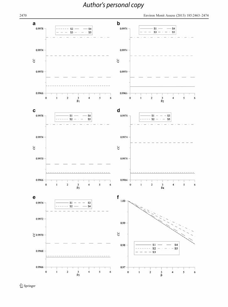
For the case study under assumption 2, the follow-ing schemes were designed. Perturbances were im-posed on the indices of the first sample with thesame ratio, and then the final CC values were recalcu-lated using Visual Basic program. The variation ratiosranged from 0.01 to 6.00 with an increment of 0.01,and the CC values were recalculated for each variationratio (the CC values were recalculated 600 times foreach sample). After that, the second sample was im-posed a perturbance, and also the variation ratiosranged from 0.01 to 6.00 with an increment of 0.01.The similar procedures were also applied to the third,fourth and fifth sample. As a result, a total of 3,000calculations were made in the case study. After theresults have been obtained, they are arranged inMicrosoft Excel and made into figures in GoldenSoftware Grapher 8. The figures illustrating the CCvalues of different samples against variation ratios (βk)are shown in Fig. 1.

& Discussion

It can be concluded from Fig. 1a to e that thevariations of the input data of a given sample haveno significant influence on the CC values of theunperturbed samples. For example, Fig. 1a illus-trated the variations of S2, S3, S4, and S5 whenthe input data of S1 had been perturbed. Althoughthe variation ratios (can be regarded as the degreeof the perturbance) ranged from 0.01 to 6.00, theCC values of S2, S3, S4, and S5 kept ratherstable. This can also be verified by Fig. 2b to e.Because the CC values of the unperturbed samplesare rarely changed, their relative orders ordered bythe CC values are also unchanged.

Figure 1f reveals that the CC values of the per-turbed samples show a linear decrease tendency withthe increase of variation ratios. In the study, the CCvalues of the five perturbed samples were shown in afigure (Fig. 1f) to check their similarities and differ-ences. It can be found from Fig. 1f that the CC values

of the five perturbed samples decrease linearly withdifferent slopes. The five linear functions can beobtained from the calculated data. According toFormula (17), 1

CC*p¼ f C; bkð Þ þ 1. For a given initial

matrix C, the function f(C, βk) changes into f(βk).

Therefore, we can define CC*p ¼ F C; bkð Þ and for a

given initial matrix C, CC*p ¼ F bkð Þ. According to the

definition, five linear functions were calculated fromthe data using least square method and they are:

F b1ð Þ ¼ �0:0033b1þ1 ð23Þ

F b2ð Þ ¼ �0:0032b2þ1 ð24Þ

F b3ð Þ ¼ �0:0027b3þ1 ð25Þ

F b4ð Þ ¼ �0:0031b4þ1 ð26Þ

F b5ð Þ ¼ �0:0024b5þ1 ð27Þ

All the five functions are perfectly fitted with highcorrelation coefficient (r201). The five functions canbe written in a uniform form, that is,

F bkð Þ ¼ akbkþ1 ð28ÞWhere, F(βk) represents the CC value of sample k,ak is a constant which denotes the slope of thefunction, βk is the variation ratio of the initial inputdata of sample k. It can be concluded from Eq. (28)that the sensitivity becomes intensive with the in-crease of the absolute value of ak. Thus, the orderof sensitivity of the five perturbed samples is S1>S2>S4>S3>S5.

Another conclusion can be reached by comparingFunctions (17), (20), and (28). Since CC*p0F(βk), wehave 1/F(βk)01/CC*p0 f(βk) + 1, and then we canknow that:

1

CC*p

¼ 1

F bkð Þ ¼1

akbk þ 1¼ � akbk

akbk þ 1þ 1 ð29Þ

f bkð Þ ¼ � akbkakbk þ 1

ð30Þ



As a result, Eq. (20) can be simply expressed as Eq.(31):

f bkð Þ ¼


bk ckj�cmjð Þ2Pmi¼1;i6¼k

cijð Þ2�

þ bk ckjð Þ2


bk ckj�cljð Þ2Pmi¼1;i6¼k

cijð Þ2�

þ bk ckjð Þ2

vuuut¼ � akbk

akbk þ 1

ð31ÞWhere, ak is a number determined by the initial

decision matrix C with nonlinear relationship. It isalso influenced by the sample on which the perturb-ance is imposed. The slope ak can be determined bytwo calculations when the perturbed sample has beendetermined. Therefore, a conclusion can be madefrom Eq. (31) that for a given initial decision ma-trix, once the perturbed sample has been identified,the final CC values of the perturbed samples atdifferent variation ratios can be determined by twocalculations. This conclusion is only valid for case2, and for cases 1, 3, and 4 it is difficult to obtainsimilar simple equations.

Although similar equations for cases 1, 3, and 4cannot be obtained easily, the conclusion reachedabove is still quite useful in determining the orders

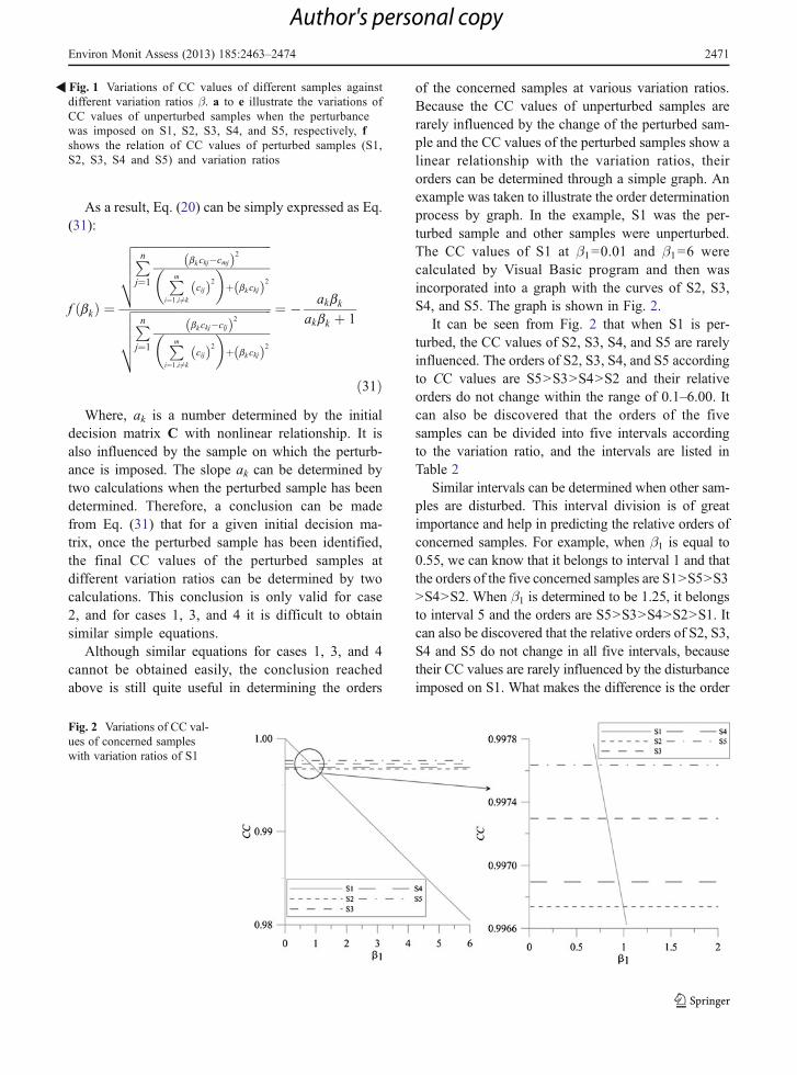
of the concerned samples at various variation ratios.Because the CC values of unperturbed samples arerarely influenced by the change of the perturbed sam-ple and the CC values of the perturbed samples show alinear relationship with the variation ratios, theirorders can be determined through a simple graph. Anexample was taken to illustrate the order determinationprocess by graph. In the example, S1 was the per-turbed sample and other samples were unperturbed.The CC values of S1 at β100.01 and β106 werecalculated by Visual Basic program and then wasincorporated into a graph with the curves of S2, S3,S4, and S5. The graph is shown in Fig. 2.

It can be seen from Fig. 2 that when S1 is per-turbed, the CC values of S2, S3, S4, and S5 are rarelyinfluenced. The orders of S2, S3, S4, and S5 accordingto CC values are S5>S3>S4>S2 and their relativeorders do not change within the range of 0.1–6.00. Itcan also be discovered that the orders of the fivesamples can be divided into five intervals accordingto the variation ratio, and the intervals are listed inTable 2

Similar intervals can be determined when other sam-ples are disturbed. This interval division is of greatimportance and help in predicting the relative orders ofconcerned samples. For example, when β1 is equal to0.55, we can know that it belongs to interval 1 and thatthe orders of the five concerned samples are S1>S5>S3>S4>S2. When β1 is determined to be 1.25, it belongsto interval 5 and the orders are S5>S3>S4>S2>S1. Itcan also be discovered that the relative orders of S2, S3,S4 and S5 do not change in all five intervals, becausetheir CC values are rarely influenced by the disturbanceimposed on S1. What makes the difference is the order

Fig. 2 Variations of CC val-ues of concerned sampleswith variation ratios of S1

�Fig. 1 Variations of CC values of different samples againstdifferent variation ratios β. a to e illustrate the variations ofCC values of unperturbed samples when the perturbancewas imposed on S1, S2, S3, S4, and S5, respectively, fshows the relation of CC values of perturbed samples (S1,S2, S3, S4 and S5) and variation ratios



of S1. The CC value of S1 decreases linearly, whichdisrupts the orders of the five samples.

Limitations and future prospects

The present study, although is very meaningful boththeoretically and practically, does has its limitations,and further studies are expected in the near future. Thelimitations of the present study are summarized asfollows.

& The assumptions proposed in the present studywere very ideal. Practically, the indices of differentsamples will vary with different ratios rather thanwith the same ratios as was assumed in the presentstudy. Similarly, the indices within a given samplewill not change simultaneously with the same ra-tios, either. Therefore, the sensitivity analysis un-der different variation ratios is expected.

& In the present study, it was assumed that only oneindex (assumption 1) or only one sample (assump-tion 2) was disturbed each time. The theoreticalanalysis has indicated that under assumption 1 evenmore indices are perturbed, the final results will stillnot be influenced as long as the variation ratio is thesame with respect to the same index. However, thesame conclusion cannot be reached under assump-tion 2. Hence, a future study on the sensitivity ofTOPSIS under the condition that more samples areperturbed at the same time is required.

& It is supposed under assumption 2 that the positiveand negative ideal reference points will not bechanged by the perturbance imposed on the indicesof a given sample. For doing this, assumed positiveand negative ideal reference points were predeter-mined before analysis. Practically, the positive andnegative ideal reference points should be selectedfrom the weighted normalized decisionmatrix. If the

indices of a given sample change, the positive andnegative ideal reference points might also change.Future study on the impacts of the change of thepositive and negative ideal reference points on thefinal calculation results should be implemented.

Conclusions

Sensitivity analysis is becoming more and more pop-ular in various fields and is an essential step formultiple-criteria decision-making process. In the pres-ent study, the sensitivity of the TOPSIS method to theindex input data of water samples was investigated.The sensitivity was firstly analyzed theoretically undertwo assumptions, and then a case study under assump-tion 2 was carried out for further analysis and valida-tion. The following conclusions can be reached.

& When the same indices of different water samplesare changed simultaneously with the same varia-tion ratio, the perturbance will have influence nei-ther on the CC values of all samples, nor on thesample orders ordered by the CC values, andtherefore the final water quality assessment resultswill not be influenced.

& When the concerned indices of a given sample areperturbed with the same variation ratio, the CCvalues of all samples will be influenced theoretical-ly. However, the influence on the disturbed sampleis much greater than that on the undisturbed sam-ples. The formulas for calculating CC values underdifferent variation ratios can be expressed in fourdifferent forms as per which sample is perturbed.However, the expressing formulas are nonlinear andcomplex, and thus are difficult for practical uses.

& The case study under assumption 2 reveals thatwhen the indices of a given sample are perturbed,the CC values of the unperturbed samples arehardly influenced and therefore the relative ordersof the unperturbed samples are unchanged.However, the influence on the perturbed sampleis much more significant and the CC values of theperturbed sample show a linear relationship with thevariation ratios. A simple linear equation is derived forthe perturbed sample and it can be used for determin-ing the sample orders under various variation ratios.Five intervals can be divided according to the varia-tion ratio based on the derived linear equation.

Table 2 Intervals divided according to the variation ratio

Interval no. Intervals Orders of the concernedsamples according to CC

1 β1≤0.72 S1>S5>S3>S4>S2

2 0.72<β1≤0.82 S5>S1>S3>S4>S2

3 0.82<β1≤0.92 S5>S3>S1>S4>S2

4 0.92<β1≤0.99 S5>S3>S4>S1>S2

5 β1>0.99 S5>S3>S4>S2>S1



& The TOPSIS method applied in water quality as-sessment is only sensitive to the variation of param-eter input data of the perturbed sample. This wouldbe helpful in reducing some uncertainties and keep-ing the assessment results stable. Therefore, we canpreliminarily conclude that the TOPSIS is a reliableand feasible method for water quality assessment.

& The present study was performed under two majorassumptions which are very ideal. There are somelimitations such as the variation ratio keeping thesame, only one index or one sample being per-turbed, and the positive/negative ideal referencepoints keeping unchanged. Especially under as-sumption 2, only one sample was perturbed eachtime. It is still unknown how the final results willbe influenced if two or more samples are perturbedsimultaneously. Hence, further studies on the sen-sitivity to the input data of more samples areexpected. Besides, the relationships between CCvalues of the undisturbed samples and the varia-tion ratios were not studied, although the linearrelationship of CC values of the perturbed sampleagainst the variation ratios was derived. Theseissues should be studied in the future.

Acknowledgments The research was supported by the DoctorPostgraduate Technical Project of Chang’an University(CHD2011ZY025 and CHD2011ZY022), the Special Fund forBasic Scientific Research of Central Colleges (CHD2011ZY020),and the National Natural Science Foundation of China(41172212). The editor and anonymous reviewers are also greatlyacknowledged for their useful comments which have helped us toimprove the quality of our paper.

References

Afshar, A., Mariño, M. A., Saadatpour, M., & Afshar, A. (2011).Fuzzy TOPSIS multi-criteria decision analysis applied toKarun reservoirs system. Water Resources Manage, 25,545–563. doi:10.1007/s11269-010-9713-x.

Awasthi, A., Chauhan, S. S., Omrani, H., & Panahi, A. (2011). Ahybrid approach based on SERVQUAL and fuzzy TOPSISfor evaluating transportation service quality. Computers andIndustrial Engineering, 61, 637–646. doi:10.1016/j.cie.2011.04.019.

Cacuci, D. G. (2003). Sensitivity and uncertainty analysis, vol-ume I: theory. Boca Raton: Chapman & Hall/CRC.

Cacuci, D. G., & Ionescu-Bujor, M. (2004). A comparativereview of sensitivity and uncertainty analysis of large-scale systems. II: statistical methods. Nuclear Science andEngineering, 147(3), 204–217.

Cacuci, D. G., Ionescu-Bujor, M., & Navon, I. M. (2005).Sensitivity and uncertainty analysis, volume II: applica-tions to large-scale systems. Boca Raton: Taylor & Francis.

Chen, T. Y. (2012). Comparative analysis of SAW and TOPSISbased on interval-valued fuzzy sets: discussions on scorefunctions and weight constraints. Expert Systems withApplications, 39, 1848–1861. doi:10.1016/j.eswa.2011.08.065.

Hwang, C. L., & Yoon, K. (1981). Multiple attribute decisionmaking methods and applications. Heidelberg: Springer.

Hyde, K. M., Maier, H. R., & Colby, C. B. (2005). A distance-based uncertainty analysis approach to multi-criteria deci-sion analysis for water resource decision making. Journalof Environmental Management, 77, 278–290. doi:10.1016/j.jenvman.2005.06.011.

Ionescu-Bujor, M., & Cacuci, D. G. (2004). A comparativereview of sensitivity and uncertainty analysis of large-scale systems. I: deterministic methods. Nuclear Scienceand Engineering, 147(3), 189–203.

Li, P. Y., Qian, H., & Wu, J. H. (2011a). Hydrochemical forma-tion mechanisms and quality assessment of groundwaterwith improved TOPSIS method in Pengyang CountyNorthwest China. E-Journal of Chemistry, 8(3), 1164–1173.

Li, P. Y., Wu, J. H., & Qian, H. (2011b). Groundwater qualityassessment based on rough sets attribute reduction andTOPSIS method in a semi-arid area, China. EnvironmentalMonitoring and Assessment. doi:10.1007/s10661-011-2306-1. Online First.

Manache, G., & Melching, C. S. (2004). Sensitivity analysis of awater-quality model using Latin hypercube sampling.Journal of Water Resources Planning and Management,130(3), 232–242. doi:10.1061/(ASCE)0733-9496(2004)130:3(232).

Nakane, K., & Haidary, A. (2010). Sensitivity analysis of streamwater quality and land cover linkage models using MonteCarlo method. International Journal Environment Resour-ces, 4(1), 121–130.

Opricovic, S., & Tzeng, G. H. (2004). Compromise solution byMCDM methods: a comparative analysis of VIKOR andTOPSIS. European Journal of Operational Research, 156,445–455. doi:10.1016/S0377-2217(03)00020-1.

Rickwood, C. J., & Carr, G. M. (2009). Development andsensitivity analysis of a global drinking water quality in-dex. Environmental Monitoring and Assessment, 156, 73–90. doi:10.1007/s10661-008-0464-6.

Sadi-Nezhad, S., & Damghani, K. K. (2010). Application of afuzzy TOPSIS method base on modified preference ratioand fuzzy distance measurement in assessment of trafficpolice centers performance. Applied Soft Computing, 10,1028–1039. doi:10.1016/j.asoc.2009.08.036.

Sun, C. C. (2010). A performance evaluation model by integrat-ing fuzzy AHP and fuzzy TOPSIS methods. Expert Sys-tems with Applications, 37, 7745–7754. doi:10.1016/j.eswa.2010.04.066.

Wang, J. R., Fan, K., &Wang, W. S. (2010). Integration of fuzzyAHP and FPP with TOPSIS methodology for aeroenginehealth assessment. Expert Systems with Applications, 37,8516–8526. doi:10.1016/j.eswa.2010.05.024.

Xu, S. L., & Xue, S. (1994). The sensitivity comprehensiveindex of environmental quality (CIEQ): with an analysis



http://dx.doi.org/10.1007/s11269-010-9713-x

http://dx.doi.org/10.1016/j.cie.2011.04.019

http://dx.doi.org/10.1016/j.cie.2011.04.019

http://dx.doi.org/10.1016/j.eswa.2011.08.065


http://dx.doi.org/10.1016/j.jenvman.2005.06.011

http://dx.doi.org/10.1016/j.jenvman.2005.06.011

http://dx.doi.org/10.1007/s10661-011-2306-1

http://dx.doi.org/10.1007/s10661-011-2306-1

http://dx.doi.org/10.1061/(ASCE)0733-9496(2004)130:3(232)

http://dx.doi.org/10.1061/(ASCE)0733-9496(2004)130:3(232)

http://dx.doi.org/10.1016/S0377-2217(03)00020-1

http://dx.doi.org/10.1007/s10661-008-0464-6

http://dx.doi.org/10.1016/j.asoc.2009.08.036




of current CIEQs. Acta Scientiae Circumstantiae, 14(3),269–274 (in Chinese).

Yang, X. H., Yang, Z. F., & Shen, Z. Y. (2004). An ideal intervalmethod of multi-objective decision-making for compre-hensive assessment of water resources renewability. Sci-ence in China, Series E, 47(S1), 42–49. doi:10.1360/04ez0004.

Yang, X. H., She, D. X., Yang, Z. F., Tang, Q. H., & Li, J. Q.(2009). Chaotic Bayesian method based on multiple criteriadecision making (MCDM) for forecasting nonlinear

hydrological time series. International Journal of NonlinearSciences and Numerical Simulation, 10(11–12), 1595–1610.

Yang, X. H., Zhang, X. J., & Hu, X. X. (2011). Nonlinear Opti-mization Set Pair Analysis Model (NOSPAM) for assessingwater resource renewability. Nonlinear Processes in Geo-physics, 18, 599–607. doi:10.5194/npg-18-599-2011.

Yuan, S. J., Wang, Q. R., Fan, S. Y., & Li, X. Q. (1998).Analysis of the sensitivity of the index method used inenvironmental quality assessment. Journal of JianghanPetroleum Institute, 20(3), 66–70 (in Chinese).



http://dx.doi.org/10.1360/04ez0004

http://dx.doi.org/10.1360/04ez0004

http://dx.doi.org/10.5194/npg-18-599-2011

Sensitivity analysis of TOPSIS method in water quality assessment II: sensitivity to the index input...

Documents

Transcript of Sensitivity analysis of TOPSIS method in water quality assessment II: sensitivity to the index input...