Sensitivity analysis of the tree distribution modelPHENOFIT to climatic input characteristics: implications forclimate impact assessment

X AV I E R M O R I N and I S A B E L L E C H U I N E

Centre d’Ecologie Fonctionnelle et Evolutive, Equipe BIOFLUX, CNRS, 1919 route de Mende, 34293 Montpellier cedex 5,

France

Abstract

Species distributions are already affected by climate change. Forecasting their long-term

evolution requires models with thoroughly assessed validation. Our aim here is to

demonstrate that the sensitivity of such models to climate input characteristics may

complicate their validation and introduce uncertainties in their predictions. In this study,

we conducted a sensitivity analysis of a process-based tree distribution model PHENOFIT

to climate input characteristics. This analysis was conducted for two North American

trees which differ greatly in their distribution and eight different types of climate input

for the historic period which differ in their spatial (local or gridded data) and temporal

(daily vs. monthly) resolution as well as their type (locally recorded, extrapolated or

simulated by General Circulation Models). We show that the climate data resolution

(spatial and temporal) and their type, highly affect the model predictions. The sensitivity

analysis also revealed, the importance, for global climate change impact assessment, of

(i) the daily variability of temperatures in modeling the biological processes shaping

species distribution, (ii) climate data at high latitudes and elevations and (iii) climate

data with high spatial resolution.

Keywords: climate change, general circulation model, plant distribution, process-based model,

sensitivity analysis

Received 9 September 2004; revised version received 7 December 2004 and accepted 15 March 2005

Introduction

Concern about the current climate change is increasing,

probably because ecological (Walther et al., 2001;

Parmesan & Yohe, 2003; Root et al., 2003), as well as

socio-economic (Michaelis, 1994; Keeney & Mc Daniels,

2001; Yohe & Schlesinger, 2002) impacts are more and

more perceptible. Climate change is significantly

affecting species development timing (Menzel & Fa-

bian, 1999; Walther et al., 2001; Parmesan & Yohe, 2003),

physiology (Keeling et al., 1996; Myneni et al., 1997;

Cannell et al., 1998; Hughes, 2000), competition

(Hughes, 2000) and geographical ranges (Parmesan

et al., 1999; Walther et al., 2002; Parmesan & Yohe, 2003)

with major consequences on biodiversity, silviculture

and agriculture (Nicholis, 1997; Jingyun et al., 2001).

The development of accurate predictive models is,

therefore, urgent to anticipate harmful consequences

and alert stake-holders. Predicting changes in plant

distribution and phenology is also a key requirement to

forecast accurately future climate because of the

vegetation’s feedback on the atmosphere (Betts et al.,

1997; de Noblet, 2000).

Climate’s impact on species’ distribution has been for

long attested (Holdridge, 1947; Budyko, 1974) and used

to reconstitute paleoclimates from information on

species past distributions (Guiot, 1994). This relation-

ship has been a basis for numerous models in ecology,

and especially in biogeography (Austin, 1985, 1999,

2002; Stephenson, 1990; Prentice et al., 1992; Brzeziecki

et al., 1993; Neilson, 1995; Kleidon & Mooney, 2000;

Chuine & Beaubien, 2001; Dullinger et al., 2004; Thuiller

et al., 2003). A few models have already been used to

predict the impact of climate change on species and

ecosystems distribution and functioning using General

Circulation Models (GCMs) predictions for the 21st

century (Huntley et al., 1995; Iverson et al., 1999; Shafer

et al., 2001; Bakkenes et al., 2002; Beaumont & Hughes,

2002; Berry et al., 2002; Erasmus et al., 2002; LehmannCorrespondence: Xavier Morin, tel. 1 33 4 67 61 32 37,

fax 1 33 4 67 41 21 38, e-mail: xavier.morin@cefe.cnrs.fr

Global Change Biology (2005) 11, 1493–1503, doi: 10.1111/j.1365-2486.2005.00996.x

r 2005 Blackwell Publishing Ltd 1493

et al., 2002; Pearson et al., 2002; Peterson et al., 2002;

Pearson & Dawson, 2003; Raxworthy et al., 2003;

Thuiller, 2003, 2004; Thomas et al., 2004; Thuiller et al.,

2004).

Two main kinds of models have been developed to

study species distribution and predict species distribu-

tion change: models based on the correspondence

between species observed distributions and environ-

mental variables (i.e. niche-based models), and models

based on the mechanisms involved in the delimitation

of species distribution (i.e. process-based models).

Providing accurate predictions for the future with such

models requires first a robust validation and second a

quantification of the different possible sources of

variation in their predictions (Rykiel, 1996; Aspinall,

2002; Fleishman et al., 2003).

In the field of ecological modeling, model validation

is of primary importance and is most discussed (Loehle,

1983; Oreskes et al., 1994; Rykiel, 1996). Several studies

concluded that crossvalidation, (i.e.) validation with an

independent data set, is the most robust and straight-

forward validation method for predictive models

(Lebreton et al., 1992) and especially for biogeography

models (Guisan & Zimmermann, 2000). Validation is

easy for process-based models as observed distribu-

tions are not used to fit the model parameters and can

be used to validate the model. It does not correspond to

a crossvalidation senso-stricto as the data used to fit the

model parameters and the data used to test the model

are of different kind. Crossvalidation is on the contrary

very difficult for niche-based models as the observed

distribution is used to fit the model parameters. The use

of half of the distribution chosen randomly to fit the

model and the other half to validate it does not provide

a robust validation as both data sets could be strongly

auto-correlated. However, the use of one continuous

part of the distribution to fit and the rest to validate

does not provide an accurate model fit either. Valida-

tion is, therefore, an important problem for niche-based

models, which is currently driving most attention

(Thuiller, 2003, 2004). Nevertheless, few biological

models aimed to provide predictions under global

change scenarios, either niche-based or process-based

are crossvalidated.

Quantifying the different sources of variation in the

model predictions has, on the contrary, very rarely been

addressed. Recently, Thuiller (2003, 2004) showed that

intrinsic sources of variation in niche-based models

could be responsible for much higher variance in the

model projections than the climate scenarios. In the

present study, we focus on the extrinsic sources of

variation that may affect model predictions, (i.e.

variation in the model’s inputs). Apart from the

accuracy of the information on the species distribution

that alters niche-based models fit and process-based

models validation, a first source of variation in the

model predictions for the future is the climate

scenarios. Several scenarios actually need to be con-

sidered to provide a range of possible outcomes. A

second source of variation in the model predictions is

the GCMs simulated climate. This source of variation

can be partly taken into account using the GCM specific

anomalies, (i.e. the differences between simulated and

observed historic climate), to correct the simulated

future climate. As these anomalies may not be constant

through time, the use of raw data should be preferred

when the simulated historic climate does not differ

substantially from the observed one. Just like for

scenarios, several GCMs should also be used to assess

climate change impacts. A third source of variation in

the model predictions is the climatic variables used in

the modeling. This source of variation has to our

knowledge never been questioned. If sensitivity ana-

lyses are sometimes undertaken on the model para-

meters, they rarely concerned the input variables

(Bachelet et al., 1998).

This last source of variation especially concerns

process-based models (vegetation functioning or bio-

geography), as an increasing number of them use daily

climatic data to simulate key biological processes

(Neilson, 1995; Kleidon & Mooney, 2000; Chuine &

Beaubien, 2001). Gridded daily climate data do not exist

at a global scale with a high spatial resolution and for

the 20th century, and are only recently available for

GCM runs at a low spatial resolution. For these reasons,

modelers have been using monthly means, either

generating, when required, the daily variability or

adapting the models to run with monthly means.

Here we aim to (i) determine the impact of the type

(locally recorded, interpolated or simulated), as well as

the spatial and temporal resolution of climate data on

the predictions of the process-based model, PHENOFIT

(Chuine & Beaubien, 2001) and (ii) identify the most

relevant type of data set to simulate species’ distribu-

tions at a continental scale (i.e. our model’s scale). For

that purpose, we conducted a sensitivity analysis of the

model to the climate input characteristics over 1950–

2000. The model originally uses daily climatic data and

generates tree species distributions. It has been pre-

viously validated for two species, quaking aspen

(Populus tremuloides Michx) and sugar maple (Acer

saccharum Marsh), using daily climate data from 92

weather stations located all over North America. The

comparison of pairs of simulations of sugar maple and

quaking aspen distributions obtained with different

types of climatic data allowed quantifying the five

following effects on the model predictions: temporal

resolution of temperature and water balance, extra-

1494 X . M O R I N & I . C H U I N E

r 2005 Blackwell Publishing Ltd, Global Change Biology, 11, 1493–1503

polation of temperatures from stations to gridded data,

generation of daily temperatures with a weather

generator and simulation of climatic data with GCMs.

Sugar maple and quaking aspen were chosen for the

complementary of their distributions, which cover

altogether a very large part of North America and

allowed the identification of geographical patterns in

the investigated effects. Although the size of these effects

may vary from one model to another, either process-

based or not, our aim is also to point out the impact of

climate data characteristics on the predictions of models

designed to assess the impact of climate change.

Material and methods

PHENOFIT

PHENOFIT is a process-based model that predicts tree

species distributions. It relies on the principle that the

adaptation of a tree species to the environmental

conditions strongly depends on the synchronization of

its timing of development to the seasonal variations of

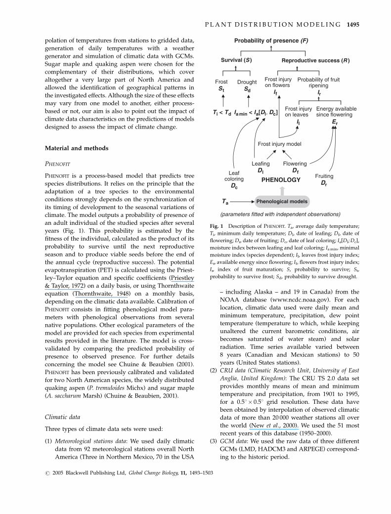
climate. The model outputs a probability of presence of

an adult individual of the studied species after several

years (Fig. 1). This probability is estimated by the

fitness of the individual, calculated as the product of its

probability to survive until the next reproductive

season and to produce viable seeds before the end of

the annual cycle (reproductive success). The potential

evapotranspiration (PET) is calculated using the Priest-

ley–Taylor equation and specific coefficients (Priestley

& Taylor, 1972) on a daily basis, or using Thornthwaite

equation (Thornthwaite, 1948) on a monthly basis,

depending on the climatic data available. Calibration of

PHENOFIT consists in fitting phenological model para-

meters with phenological observations from several

native populations. Other ecological parameters of the

model are provided for each species from experimental

results provided in the literature. The model is cross-

validated by comparing the predicted probability of

presence to observed presence. For further details

concerning the model see Chuine & Beaubien (2001).

PHENOFIT has been previously calibrated and validated

for two North American species, the widely distributed

quaking aspen (P. tremuloides Michx) and sugar maple

(A. saccharum Marsh) (Chuine & Beaubien, 2001).

Climatic data

Three types of climate data sets were used:

(1) Meteorological stations data: We used daily climatic

data from 92 meteorological stations overall North

America (Three in Northern Mexico, 70 in the USA

– including Alaska – and 19 in Canada) from the

NOAA database (www.ncdc.noaa.gov). For each

location, climatic data used were daily mean and

minimum temperature, precipitation, dew point

temperature (temperature to which, while keeping

unaltered the current barometric conditions, air

becomes saturated of water steam) and solar

radiation. Time series available varied between

8 years (Canadian and Mexican stations) to 50

years (United States stations).

(2) CRU data (Climatic Research Unit, University of East

Anglia, United Kingdom): The CRU TS 2.0 data set

provides monthly means of mean and minimum

temperature and precipitation, from 1901 to 1995,

for a 0.51� 0.51 grid resolution. These data have

been obtained by interpolation of observed climatic

data of more than 20 000 weather stations all over

the world (New et al., 2000). We used the 51 most

recent years of this database (1950–2000).

(3) GCM data: We used the raw data of three different

GCMs (LMD, HADCM3 and ARPEGE) correspond-

ing to the historic period.

Survival (S ) Reproductive success (R )

Phenological models

(parameters fitted with independent observations)

Ta

PHENOLOGY

LeafingDl

FloweringD f

FruitingDr

Frost injury model

FrostS t

DroughtSd

Frost injuryon flowers

If

Probability of fruitripening

Ir

II Er

Frost injuryon leaves

Probability of presence (F)

Ia min < Ia[Dl , Dc]

Leafcoloring

Dc

Energy availablesince floweringTi < Td

Fig. 1 Description of PHENOFIT. Ta, average daily temperature;

Ti, minimum daily temperature; Dl, date of leafing; Df, date of

flowering; Dr, date of fruiting; Dc, date of leaf coloring; Ia[Dl; Dc],

moisture index between leafing and leaf coloring; Ia min, minimal

moisture index (species dependent); Il, leaves frost injury index;

Er, available energy since flowering; If, flowers frost injury index;

Ir, index of fruit maturation; S, probability to survive; St,

probability to survive frost; Sd, probability to survive drought.

P L A N T D I S T R I B U T I O N M O D E L I N G 1495

r 2005 Blackwell Publishing Ltd, Global Change Biology, 11, 1493–1503

LMD data (Laboratoire de Meteorologie Dynamique,

CNRS, France): The LMD data consist of daily mean

and minimum temperature and daily precipitation

simulated for a 10-year period, (i.e. with 1990s

atmospheric CO2 concentration). The grid resolution

varies with latitude (narrower near the equator and

wider near the poles), and is 2.31� 3.51 on average

over North America.

HADCM3 data (Hadley Center for Climate Predictions

and Research, United Kingdom): The HADCM3 data

consist of daily mean and minimum temperatures

and daily precipitation, simulated for a 21-year

period (1980–2000). The spatial resolution is

2.51� 3.751 and is constant.

ARPEGE data (Meteo-France, France): The ARPEGE

data consist of daily mean and minimum tempera-

tures and daily precipitation, simulated for a 21-year

period (1980–2000). The spatial resolution is

2.791� 2.81251 and is constant.

The data from the meteorological stations were our

reference to quantify the different effects. The model

simulations were thus conducted with the data from

the 92 grid cells of CRU and GCMs corresponding to

the 92 meteorological stations. As the GCMs grid cells

were much larger than the CRU grid cells, we

disaggregated the GCM temperatures at the CRU

resolution with an elevation adjustment.

Characteristics of the climatic data sets are summar-

ized in Table 1.

The simulations

The different simulations were conducted as follows:

Simulation 1 (S1): Daily mean and minimum tem-

perature, precipitation, snow, dew point, radiation

recorded at the 92 meteorological stations were used.

These data allow for the Priestley–Taylor’s PET

calculation (Priestley & Taylor, 1972) and provide a

daily PET.

Simulation 2 (S2): Daily mean and minimum tem-

perature and monthly precipitation recorded at the

92 stations were used. The PET is calculated with

Thornthwaite’s equation (Thornthwaite, 1948) to

provide a monthly PET.

All subsequent simulations (S3–S6) used monthly

mean precipitation and PET.

Simulation 3 (S3): Observed monthly mean tempera-

tures of the 92 meteorological stations (temperature

constant for each day of a month), and corresponding

monthly mean precipitation were used.

Simulation 4 (S4): Daily mean and minimum tem-

peratures generated from the monthly means of the

92 meteorological stations, and corresponding

monthly mean precipitation were used.

Simulation 5 (S5): Daily mean and minimum tem-

peratures generated from extrapolated monthly

means (CRU database), and corresponding monthly

mean precipitation were used.

Simulations 6a, 6b and 6c (S6a, S6b, S6c): Raw daily

mean and minimum temperatures, and precipitation

simulated by the LMD (S6a), HADCM3 (S6b) and

ARPEGE (S6c) GCMs for the historic period were

used.

Simulations are summarized in Table 2.

The comparison of five pairs of these simulations

allowed for the discrimination of the following five

effects:

(1) monthly (S2) vs. daily (S1) water balance;

(2) monthly (S3) vs. daily (S2) mean temperatures;

(3) generated (from observed monthly means) (S4) vs.

observed (S2) daily temperatures;

(4) extrapolated (CRUs data) (S5) vs. observed (S4)

monthly mean temperatures;

(5) raw GCMs (S6a, S6b, S6c) vs. observed (S2) climate.

Effects tested are summarized in Table 3.

Table 1 Characteristics of the climatic data sets used

Data set

Spatial

resolution Period (year) Simulation

Weather

Stations

Local 50 (1949–1998)* S1, S2, S3, S4

CRU 0.51� 0.51 50 (1951–2000) S5

LMD 2.31� 3.51 10 (1�CO2) S6a

HADCM3 2.51� 3.751 21 (1980–2000) S6b

ARPEGE 2.791� 2.81251 21 (1980–2000) S6c

*Eight years (1991–1998) for three Mexican stations and 19

Canadian stations.

Table 2 Summarized description of the simulations

Simulations Data set Temperatures PET

S1 Weather stations Daily, observed Daily

S2 Weather stations Daily, observed Monthly

S3 Weather stations Monthly, observed Monthly

S4 Weather stations Daily, generated* Monthly

S5 CRU Daily, generated* Monthly

S6a Raw LMD Daily, simulated Monthly

S6b Raw HADCM3 Daily, simulated Monthly

S6c Raw ARPEGE Daily, simulated Monthly

*From the monthly means.

1496 X . M O R I N & I . C H U I N E

r 2005 Blackwell Publishing Ltd, Global Change Biology, 11, 1493–1503

Method for generating daily temperatures from monthlymeans

We followed the classical and simple method of

generation of daily temperature from monthly means

used by several weather generators, (e.g. CLIGEN

(Nicks et al., 1995)). Daily values of a given variable of

month i of year j were obtained by a random draw from

the normal distribution N(mi,j,si,j) with mi,j the monthly

mean of the variable. The standard error si,j was

randomly drawn from the normal distribution

N0(mi’,si’), where mi’ and si’ are, respectively, the mean

and the standard error of the monthly standard errors.

Random draws were obtained with the Marsaglia et al.

(1990) procedure.

Two sets of daily series were generated for simula-

tions 4 (S4a and S4b) and 5 (S5a and S5b) to account for

stochasticity effect. Simulations S4 and S5 results are

the means of S4a and S4b; and S5a and S5b,

respectively.

Species observed distribution

The species observed distributions consisted of digital

maps from the US Department of Agriculture Forest

Service (http://climchange.cr.usgs.gov/data/atlas/lit-

tle). These maps were compiled by Little and Critch-

field (Critchfield & Little, 1966; Little, 1971, 1976, 1977)

based on 10-year field observations.

Predictions’ accuracy and simulations comparison

A usual, yet controversial, statistics for comparing

simulated distribution maps to observed distribution

maps is the k index (Landis & Koch, 1977; Monserud &

Leemans, 1992). Indeed the use of k for quantifying

levels of agreement between observed distribution

maps and simulated distribution maps is misleading

because it breaks the condition of statistical indepen-

dence between the two distributions. Consequently, the

empirical scaling of k (40.74 excellent agreement; 0.60–

0.74 very good; 0.40–0.59 fair;o0.40 poor), which is

arbitrary, is also misleading (Landis & Koch, 1977). In

the special case of process-based models (as it is in the

present study), the condition of statistical independence

is fulfilled. However, lacking a proper framework for

the use of k in our case, we used it to rank the

simulations, but not to quantify the effects.

k requires presence/absence values. As PHENOFIT

outputs continuous values between 0 and 1, following

the classical methodology (Thuiller, 2003), we used a

cut-off threshold to assign the presence or the absence

of the species, and chose the threshold that minimized

the mean square error. As imposing a cut-off threshold

is a source of uncertainty, we also used a threshold-

independent index (i.e. the area under the relative

operating characteristics curve (AUC)). The greater the

AUC the higher the agreement (for more details, see

Fielding & Bell, 1997). AUC is ranged from 0.5 to 1, and

0.9 for instance, means very good agreements (Swets,

1988).

However, because the AUC provide a global estima-

tion of the model accuracy, do not depict local

discrepancies, and only apply to presence/absence

binary data, we also used the simulation’s likelihood

calculated as in Chuine & Beaubien (2001).

The different simulations were ranked according to

their log-likelihood L, k and AUCs. Each of the five

effects was quantified by the log likelihood ratio (LLR)

of the corresponding paired simulations (i.e. the

difference between their log-likelihood). Local differ-

ences between paired simulations at each of the 92

locations (LLR) were mapped and interpolated using

the inverse distance weighted interpolation method

(calculation on the 12 nearest neighbors) of ESRIs

ArcMapt 8.3.8.d. Interpolations have been undertaken

to help visualizing geographical patterns, but the

numerical results presented in the text and in the tables

are based on the 92 points of comparison.

Results

The log-likelihood L, k and AUC of each simulation are

shown in Table 4. The LLRs of the paired simulations

quantifying the five effects are shown in Table 5, and

local differences are shown in Fig. 2.

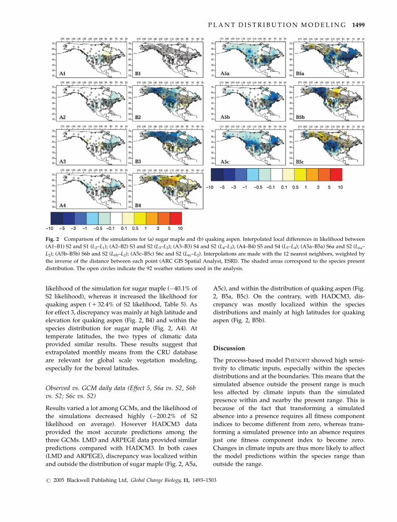
Differences between the simulations were usually

confined within the species distributions or close to

their limits except for the GCM simulations (Fig. 2), the

estimated fitness outside the present distributions

usually remaining low. For sugar maple, the simula-

tions ranked approximately in the same order whatever

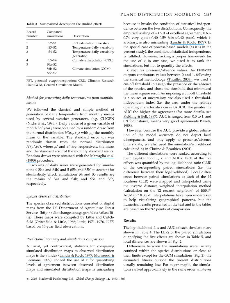
Table 3 Summarized description the studied effects

Record

number

Compared

simulations Description

1 S2–S1 PET calculation time step

2 S3–S2 Temperature daily variability

3 S4–S2 Temperature daily variability

generation

4 S5–S4 Climate extrapolation (CRU)

5 S6a–S2

S6b–S2 Climate simulation (GCM)

S6c–S2

PET, potential evapotranspiration; CRU, Climatic Research

Unit; GCM, General Circulation Model.

P L A N T D I S T R I B U T I O N M O D E L I N G 1497

r 2005 Blackwell Publishing Ltd, Global Change Biology, 11, 1493–1503

the statistics used, rank switch between L and k or AUC

(i.e. S1 and S2 or S6a and S6c) concerned simulations

with very similar L and k or AUC. For quaking aspen,

except simulation S6b (HADCM3 data) that was ranked

first by k and AUC but fifth by the likelihood,

simulations were ranked approximately the same order

by the different statistics.

Water balance calculation (Effect 1, S2 vs. S1)

L, k and AUC values show that the use of daily vs.

monthly water balance does not affect much the model

predictions (Table 4), which are slightly better with a

daily water balance except for sugar maple according to

L. The use of a monthly water balance actually provides

slightly better predictions within the distribution of

sugar maple, whereas the use of a daily water balance

provides better results in the Great Plains (west of the

distribution) where water constraints are stronger

(Fig. 2, A1). This result is in agreement with the species

sensitivity to water stress, which is very weak for

quaking aspen and a bit stronger for sugar maple. The

use of monthly water balance is thus on average as

relevant as a daily water balance at this scale.

According to this result, S2 was taken as the reference

simulation and each effect was expressed as a percen-

tage of S2 likelihood.

Daily vs. monthly temperature (Effect 2, S3 vs. S1)

The use of monthly mean temperatures instead of daily

temperatures decreased the accuracy of the predictions

sharply for both species, but especially for quaking

aspen (Table 4). The use of monthly temperatures

decreased the simulation likelihood by 50.2% of S2

likelihood for sugar maple and 69.6% for quaking

aspen (Table 5). Local differences between the two runs

were mainly marked overall the distribution of sugar

maple (Fig. 2, A2), and at high latitudes and elevations

(Rocky Mountains) of the distribution of quaking aspen

(Fig. 2, B2).

Observed vs. generated daily temperatures (Effect 3, S2vs. S4)

The daily temperature generation effect differed greatly

between the two species (Table 5). For quaking aspen

the generation of the daily variability of temperatures

reduced the likelihood of the simulation by 46.1% of S2

likelihood, discrepancy was mainly localized at high

latitudes (Fig. 2, B3). The decrease in likelihood was

much less for sugar maple (�28.3% of S2 likelihood),

and discrepancy was localized within the observed

distribution (Fig. 2, A3).

Observed monthly means vs. extrapolated monthly means(Effect 4, S5 vs. S4)

The use of extrapolated monthly means (CRU data)

instead of observed monthly means (used to generate

daily data), affected very differently the simulated

distribution of the two species. Indeed, it decreased the

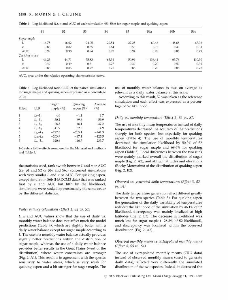
Table 4 Log-likelihood (L), k and AUC of each simulation (S1–S6c) for sugar maple and quaking aspen

S1 S2 S3 S4 S5 S6a S6b S6c

Sugar maple

L �16.75 �16.02 �24.05 �20.54 �27.25 �60.46 �48.68 �67.36

k 0.83 0.82 0.55 0.64 0.50 0.17 0.40 0.31

AUC 0.99 0.98 0.94 0.97 0.94 0.78 0.86 0.79

Quaking aspen

L �44.23 �44.71 �75.83 �65.31 �50.99 �136.41 �65.76 �110.30

k 0.49 0.49 0.31 0.27 0.39 0.20 0.50 0.39

AUC 0.86 0.85 0.77 0.75 0.85 0.70 0.88 0.78

AUC, area under the relative operating characteristics curve.

Table 5 Log-likelihood ratio (LLR) of the paired simulations

for sugar maple and quaking aspen expressed as a percentage

of L2

Effect LLR

Sugar

maple (%)

Quaking

aspen (%)

Average

(%)

1 L2–L1 4.6 �1.1 1.7

2 L3–L2 �50.2 �69.6 �59.9

3 L4–L2 �28.3 �46.1 �37.2

4 L5–L4 �41.9 32.0 �4.9

5 L6a–L2 �277.5 �205.1 �241.3

5 L6b–L2 �203.9 �47.1 �125.5

5 L6c–L2 �320.6 �146.7 �233.7

1–5 refers to the effects numbered in the Material and methods

and Table 3.

1498 X . M O R I N & I . C H U I N E

r 2005 Blackwell Publishing Ltd, Global Change Biology, 11, 1493–1503

likelihood of the simulation for sugar maple (�40.1% of

S2 likelihood), whereas it increased the likelihood for

quaking aspen ( 1 32.4% of S2 likelihood, Table 5). As

for effect 3, discrepancy was mainly at high latitude and

elevation for quaking aspen (Fig. 2, B4) and within the

species distribution for sugar maple (Fig. 2, A4). At

temperate latitudes, the two types of climatic data

provided similar results. These results suggest that

extrapolated monthly means from the CRU database

are relevant for global scale vegetation modeling,

especially for the boreal latitudes.

Observed vs. GCM daily data (Effect 5, S6a vs. S2, S6bvs. S2; S6c vs. S2)

Results varied a lot among GCMs, and the likelihood of

the simulations decreased highly (�200.2% of S2

likelihood on average). However HADCM3 data

provided the most accurate predictions among the

three GCMs. LMD and ARPEGE data provided similar

predictions compared with HADCM3. In both cases

(LMD and ARPEGE), discrepancy was localized within

and outside the distribution of sugar maple (Fig. 2, A5a,

A5c), and within the distribution of quaking aspen (Fig.

2, B5a, B5c). On the contrary, with HADCM3, dis-

crepancy was mostly localized within the species

distributions and mainly at high latitudes for quaking

aspen (Fig. 2, B5b).

Discussion

The process-based model PHENOFIT showed high sensi-

tivity to climatic inputs, especially within the species

distributions and at the boundaries. This means that the

simulated absence outside the present range is much

less affected by climate inputs than the simulated

presence within and nearby the present range. This is

because of the fact that transforming a simulated

absence into a presence requires all fitness component

indices to become different from zero, whereas trans-

forming a simulated presence into an absence requires

just one fitness component index to become zero.

Changes in climate inputs are thus more likely to affect

the model predictions within the species range than

outside the range.

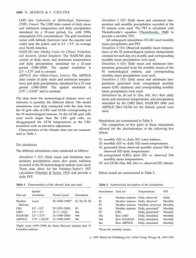
Fig. 2 Comparison of the simulations for (a) sugar maple and (b) quaking aspen. Interpolated local differences in likelihood between

(A1–B1) S2 and S1 (L2–L1); (A2–B2) S3 and S2 (L3–L2); (A3–B3) S4 and S2 (L4–L2); (A4–B4) S5 and S4 (L5–L4); (A5a–B5a) S6a and S2 (L6a–

L2); (A5b–B5b) S6b and S2 (L6b–L2); (A5c–B5c) S6c and S2 (L6c–L2). Interpolations are made with the 12 nearest neighbors, weighted by

the inverse of the distance between each point (ARC GIS Spatial Analyst, ESRI). The shaded areas correspond to the species present

distribution. The open circles indicate the 92 weather stations used in the analysis.

P L A N T D I S T R I B U T I O N M O D E L I N G 1499

r 2005 Blackwell Publishing Ltd, Global Change Biology, 11, 1493–1503

If we rank the five effects from the strongest to the

weakest according to the likelihood ratio, we end up

with (1) effect 5, GCM simulated vs. observed daily

temperatures (�200.2%, average over simulations S6a,

S6b and S6c), (2) effect 2, monthly means vs. daily

temperatures (�59.9%), (3) effect 3, generated (from

monthly means) vs. observed daily temperatures

(�7.2%), (4) effect 4, extrapolated vs. observed monthly

means (�4.9%), (5) effect 1, monthly vs. daily water

balance and PET ( 1 1.7%) (Table 5). Modeling species

distribution with PHENOFIT using daily temperatures

generated (effect 3) from extrapolated monthly means

(CRU) (effect 4), which has been and still is a common

situation, reduces the simulation likelihood by about

70.2% of S2 likelihood for A. saccharum and 14.0% for P.

tremuloides (Table 5, sum of independents effects 3 and

4) compared with using recorded daily temperatures.

PET calculation at global scale

The differences observed between simulations using

monthly PET and daily PET at a continental scale are

very small, even for the most water sensitive species,

sugar maple. At least at a continental scale, the use of

PHENOFIT with monthly PET thus appears as relevant as

with daily PET, which is fortunate as daily PET

calculation is much more difficult and requires much

more climate variables than monthly PET calculation.

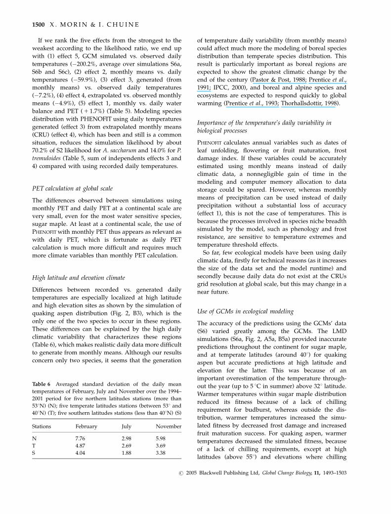
High latitude and elevation climate

Differences between recorded vs. generated daily

temperatures are especially localized at high latitude

and high elevation sites as shown by the simulation of

quaking aspen distribution (Fig. 2, B3), which is the

only one of the two species to occur in these regions.

These differences can be explained by the high daily

climatic variability that characterizes these regions

(Table 6), which makes realistic daily data more difficult

to generate from monthly means. Although our results

concern only two species, it seems that the generation

of temperature daily variability (from monthly means)

could affect much more the modeling of boreal species

distribution than temperate species distribution. This

result is particularly important as boreal regions are

expected to show the greatest climatic change by the

end of the century (Pastor & Post, 1988; Prentice et al.,

1991; IPCC, 2000), and boreal and alpine species and

ecosystems are expected to respond quickly to global

warming (Prentice et al., 1993; Thorhallsdottir, 1998).

Importance of the temperature’s daily variability inbiological processes

PHENOFIT calculates annual variables such as dates of

leaf unfolding, flowering or fruit maturation, frost

damage index. If these variables could be accurately

estimated using monthly means instead of daily

climatic data, a nonnegligible gain of time in the

modeling and computer memory allocation to data

storage could be spared. However, whereas monthly

means of precipitation can be used instead of daily

precipitation without a substantial loss of accuracy

(effect 1), this is not the case of temperatures. This is

because the processes involved in species niche breadth

simulated by the model, such as phenology and frost

resistance, are sensitive to temperature extremes and

temperature threshold effects.

So far, few ecological models have been using daily

climatic data, firstly for technical reasons (as it increases

the size of the data set and the model runtime) and

secondly because daily data do not exist at the CRUs

grid resolution at global scale, but this may change in a

near future.

Use of GCMs in ecological modeling

The accuracy of the predictions using the GCMs’ data

(S6) varied greatly among the GCMs. The LMD

simulations (S6a, Fig. 2, A5a, B5a) provided inaccurate

predictions throughout the continent for sugar maple,

and at temperate latitudes (around 401) for quaking

aspen but accurate predictions at high latitude and

elevation for the latter. This was because of an

important overestimation of the temperature through-

out the year (up to 5 1C in summer) above 321 latitude.

Warmer temperatures within sugar maple distribution

reduced its fitness because of a lack of chilling

requirement for budburst, whereas outside the dis-

tribution, warmer temperatures increased the simu-

lated fitness by decreased frost damage and increased

fruit maturation success. For quaking aspen, warmer

temperatures decreased the simulated fitness, because

of a lack of chilling requirements, except at high

latitudes (above 551) and elevations where chilling

Table 6 Averaged standard deviation of the daily mean

temperatures of February, July and November over the 1994–

2001 period for five northern latitudes stations (more than

531N) (N); five temperate latitudes stations (between 531 and

401N) (T); five southern latitudes stations (less than 401N) (S)

Stations February July November

N 7.76 2.98 5.98

T 4.87 2.69 3.69

S 4.04 1.88 3.38

1500 X . M O R I N & I . C H U I N E

r 2005 Blackwell Publishing Ltd, Global Change Biology, 11, 1493–1503

requirements were still fulfilled and frost damage

decreased.

The HADCM3 simulations provided the most accu-

rate predictions over all the GCMs either for sugar

maple or quaking aspen. The region showing the

greatest deviance from S2 is northeastern North

America for sugar maple where temperatures are

abnormally warm in winter and cold in summer

decreasing fitness because of a lack of chilling require-

ments in winter and higher risk of frost damage in late

summer. The simulated distribution of quaking aspen

was mainly affected in northwestern North America

where temperatures were abnormally cold, increasing

frost damage.

The ARPEGE simulations (S6c, Fig. 2, A5c, and B5c)

provided inaccurate predictions throughout the con-

tinent for sugar maple and in western United States for

quaking aspen. This result was because of an over-

estimation of winter temperatures in northern latitudes

(above 501 in the West and 351 in the East), and an

underestimation in southern latitudes compared with

observed climate. Colder temperatures reduced sugar

maple simulated fitness over its present distribution

because of increased frost damage and a later flower-

ing; whereas warmer temperatures increased the

species probability of presence outside its distribution

because of decreased frost damage and increased fruit

maturation success. Warmer temperatures in northern

latitudes increased quaking aspen’s probability of

presence over most of its distribution because of

decreased frost damage and increased fruit maturation

success, whereas colder temperatures in western Uni-

ted States increased the probability of presence outside

the observed distribution.

These results stress two points. Firstly, the impact of

climate change on species distribution will not be easily

assessed because climate change varies through space

and time and the climate-adapted traits limiting species

fitness vary within the species distribution. Secondly, to

predict species distribution change under climate

change scenarios with PHENOFIT, it would be recom-

mended to use specific anomalies for LMD and

ARPEGE, and raw data for HADCM3.

Simulations using GCMs’ data would probably be

more accurate if data were available at a higher spatial

resolution and for longer time spans (the GCMs time

series were much shorter than the weather stations or

CRU data, see Table 1). Spatial disaggregation of

temperatures according to elevation cannot indeed

replace temperatures generated at a high spatial

resolution by the GCMs, and short climate series are

not adequate to model long lived organisms’ distribu-

tion. Regional Circulation Models, which can provide

high spatial and temporal resolution data, will thus

have a major role to play in the assessment of global

climate change’s impact, especially on alpine and

boreal ecosystems.

Acknowledgements

The authors thank D. Viner (Climate Research Unit, Universityof East Anglia, United Kingdom), J. Polcher (Laboratoire deMeteorologie Dynamique, CNRS, France), and J.-F. Royer and A.Rascol (Meteo-France) for providing us the climate data.Observed distribution maps of quaking aspen and sugar mapleare from the USDA Forest Service. The authors are grateful to J.Roy and N. Viovy for their constructive comments, B.Hautdidier for mapping help, R. Pradel for statistical help, andalso three anonymous referees whose constructive remarkshighly increased the quality of this paper. Support was providedto X. Morin by a Bourse de Docteur Ingenieur du CentreNational de la Recherche Scientifique.

References

Aspinall RJ (2002) Use of logistic regression for validation of

maps of the spatial distribution of vegetation species derived

from high spatial resolution hyperspectral remotely sensed

data. Ecological Modelling, 157, 301–312.

Austin MP (1985) Continuum concept, ordination methods,

and niche theory. Annual Review of Ecology and Systematics, 16,

39–61.

Austin MP (1999) A silent clash of paradigms: some incon-

sistencies in community ecology. Oikos, 86, 170–178.

Austin MP (2002) Spatial prediction of species distribution: an

interface between ecological theory and statistical modelling.

Ecological Modelling, 157, 101–118.

Bachelet D, Brugnach M, Neilson RP (1998) Sensitivity of a

biogeography model to soil properties. Ecological Modelling,

109, 77–98.

Bakkenes M, Alkemade JRM, Ihle F et al. (2002) Assessing effects

of forecasted climate change on the diversity and distribution

of European higher plants for 2050. Global Change Biology, 8,

390–407.

Beaumont LJ, Hughes L (2002) Potential changes in the

distributions of latitudinally restricted Australian butterfly

species in response to climate change. Global Change Biology, 8,

954–971.

Berry PM, Dawson TP, Harrison PA et al. (2002) Modelling

potential impacts of climate change on the bioclimatic

envelope of species in Britain and Ireland. Global Ecology and

Biogeography, 11, 453–462.

Betts RA, Cox PM, Lee SE et al. (1997) Contrasting physiological

and structural vegetation feedbacks in climate change

simulations. Nature, 387, 796–799.

Brzeziecki B, Kienast F, Wildi O (1993) A simulated map of the

potential natural forest vegetation of Switzerland. Journal of

Vegetation Science, 4, 499–508.

Budyko MI (1974) Climate and Life. Academic Press, New York,

NY.

Cannell MGR, Thornley JHM, Mobbs DC et al. (1998) UK conifer

forests may be growing faster in response to increased

P L A N T D I S T R I B U T I O N M O D E L I N G 1501

r 2005 Blackwell Publishing Ltd, Global Change Biology, 11, 1493–1503

N deposition, atmospheric CO2 and temperature. Forestry, 71,

277–296.

Chuine I, Beaubien E (2001) Phenology is a major determinant of

temperate tree distributions. Ecology Letters, 4, 500–510.

Critchfield WB, Little ELJ (1966) Geographic distribution of the

pines of the world. Report No. 991. US Department of

Agriculture, 97 pp.

de Noblet N (2000) Mid-Holocene greening of the Sahara: first

results of the GAIM 6000 year BP Experiment with two

asynchronously coupled atmosphere/biome models. Climate

Dynamics, 16, 643–659.

Dullinger S, Dirnbock T, Grabherr S (2004) Modelling climate

change-driven treeline shifts: relative effects of temperature

increase, dispersal and invasibility. Journal of Ecology, 92, 241–

252.

Erasmus BFN, Jaarsveld ASv, Chown SL et al. (2002) Vulner-

ability of South African animal taxa to climate change. Global

Change Biology, 8, 679–693.

Fielding AH, Bell JF (1997) A review of methods for the

assessment of prediction errors in conservation presence/

absence models. Environmental Conservation, 24, 38–49.

Fleishman E, Nally RM, Fay JP (2003) Validation tests of

predictive models of butterfly occurrence based on environ-

mental variables. Conservation Biology, 17, 806–817.

Guiot J (1994) Statistical analyses of biospherical variability. In:

Long-Term Climatic Variations. Data and Modelling, Vol. I

(Spyridakis MT, ed.), pp. 299–334. Springer-Verlag, Berlin.

Guisan A, Zimmermann NE (2000) Predictive habitat distribu-

tion models in ecology. Ecological Modelling, 135, 147–186.

Holdridge LR (1947) Determination of world plant formations

from simple climatic data. Science, 105, 267–268.

Hughes L (2000) Biological consequences of global warming: is

the signal already apparent. Trends in Ecology and Evolution, 15,

56–61.

Huntley B, Berry MB, Cramer W et al. (1995) Modelling present

and potential future ranges of some European higher plants

using climate response surfaces. Journal of Biogeography, 22,

967–1001.

IPCC (2000) Scenarios of Climate Change for Europe. European

Commission, London.

Iverson LR, Prasad AM, Schwartz MW (1999) Modeling

potential future individual tree-species distribution in the

Eastern United States under a climate change scenario: a

case study with Pinus virginiana. Ecological Modelling, 115,

77–93.

Jingyun F, Anping C, Changhui P et al. (2001) Changes in forest

biomass carbon storage in China between 1949 and 1998.

Science, 292, 2320–2322.

Keeling CD, Chin JFS, Whorf TP (1996) Increased activity of

northern vegetation inferred from atmospheric CO2 measure-

ments. Nature, 382, 146–149.

Keeney RL, Mc Daniels TL (2001) A framework to guide

thinking and analysis regarding climate change policies. Risk

Analysis, 21, 989–1000.

Kleidon A, Mooney HA (2000) A global distribution of

biodiversity inferred from climatic constraints: results from

a process-based modelling study. Global Change Biology, 6,

507–523.

Landis JR, Koch GG (1977) The measurement of observer

agreement for categorical data. Biometrics, 33, 159–174.

Lebreton D, Burhnam KP, Clobert J (1992) Modeling survival

and testing biological hypotheses using marked animals: a

unified approach with case studies. Ecological Monographs, 62,

67–118.

Lehmann A, Overton JM, Austin MP (2002) Regression models

for spatial prediction: their role for biodiversity and conserva-

tion. Biodiversity and Conservation, 11, 2085–2092.

Little ELJ (1971) Atlas of United States trees, Vol. 1, Conifers and

important hardwoods. Report No. 1146. U.S. Department of

Agriculture, 9 pp.

Little ELJ (1976) Atlas of United States trees, Vol. 3, Minor Western

hardwoods. Report No. 1314. Department of Agriculture, 13 pp.

Little ELJ (1977) Atlas of United States trees, Vol. 4, Minor Eastern

hardwoods. Report No. 1342. Department of Agriculture, 17 pp.

Loehle C (1983) Evaluation of theories and calculation tools in

ecology. Ecological Modelling, 19, 239–247.

Marsaglia G, Zaman A, Tsang W (1990) Toward a universal

random number generator. Statistics and Probability Letters, 8,

35–39.

Menzel A, Fabian P (1999) Growing season extended in Europe.

Nature, 397, 659.

Michaelis P (1994) On the economics of greenhouse gas

accumulation: a simulation approach. European Journal of

Political Economics, 10, 707–726.

Monserud RA, Leemans R (1992) Comparing global vegetation

maps with the kappa statistics. Ecological Modelling, 63, 275–293.

Myneni RB, Keeling CD, Tucker CJ et al. (1997) Increasing plant

growth in the northern high latitudes from 1981 to 1991.

Nature, 386, 698–702.

Neilson RP (1995) A model for predicting continental-scale

vegetation distribution and water balance. Ecological Mono-

graph, 5, 362–385.

New M, Hulme M, Jones P (2000) Representing twentieth

century space-time climate variability. Part II: development of

a 1901–1996 monthly grids of terrestrial surface climate.

Journal of Climate, 13, 2217–2238.

Nicholis N (1997) Increased Australian wheat yield due to recent

climate trends. Nature, 387, 484–485.

Nicks AD, Lane LJ, Gander GA (1995) Weather generator. In:

USDA-Water Erosion Prediction Project: Hillslope Profile and

Watershed Model Documentation (Nearing MA, ed.), pp. 2.1–

2.22. NSERL West Lafayette.

Oreskes N, Shrader-Frechette K, Belitz K (1994) Verification,

validation, and confirmation of numerical models in the Earth

sciences. Science, 263, 641–646.

Parmesan C, Ryrholm N, Stefanescus C et al. (1999) Poleward

shifts in geographical ranges of butterfly species associated

with regional warming. Nature, 399, 679–583.

Parmesan C, Yohe G (2003) A globally coherent fingerprint of

climate change impacts across natural systems. Nature, 421,

37–42.

Pastor J, Post E (1988) Response of northern forests to CO2-

induced climate change. Nature, 334, 55–58.

Pearson RG, Dawson PD (2003) Predicting the impacts of climate

change on the distribution of species: are bioclimate envelope

models useful? Global Ecology and Biogeography, 12, 361–371.

1502 X . M O R I N & I . C H U I N E

r 2005 Blackwell Publishing Ltd, Global Change Biology, 11, 1493–1503

Pearson RG, Dawson TP, Berry PM et al. (2002) SPECIES: a

spatial evaluation of climate impact on the envelope of

species. Ecological Modelling, 154, 289–300.

Peterson AT, Ortega-Huerta MA, Bartley J et al. (2002) Future

projections for Mexican faunas under global climate change

scenarios. Nature, 416, 626–628.

Prentice IC, Cramer W, Harrison SP et al. (1992) A global biome

model based on plant physiology and dominance, soil

properties and climate. Journal of Biogeography, 19, 117–134.

Prentice IC, Sykes MT, Cramer W (1991) The possible dynamic

response of northern forests to global warming. Global Ecology

and Biogeography Letters, 1, 129–135.

Prentice IC, Sykes MT, Cramer W (1993) A simulation model for

the transient effect of climate change on forest landscape.

Ecological Modelling, 65, 51–70.

Priestley CHB, Taylor RJ (1972) On the assessment of surface

heat flux and evaporation using large-scale parameters.

Monthly Weather Review, 100, 81–92.

Raxworthy CJ, Martinez-Meyer E, Horning N et al. (2003)

Predicting distributions of known and unknown reptile

species in Madagascar. Nature, 426, 837–841.

Root TL, Price JT, Hall KR et al. (2003) Fingerprints of global

warming on wild animals and plants. Nature, 421, 57–60.

Rykiel EJ (1996) Testing ecological models: the meaning of

validation. Ecological Modelling, 90, 229–244.

Shafer SL, Bartlein PJ, Thompson RS (2001) Potential changes in

the distributions of Western North America tree and shrub

taxa under future climate scenarios. Ecosystems, 4, 200–215.

Stephenson NL (1990) Climatic control of vegetation distribu-

tion: the role of the water balance. The American Naturalist, 135,

649–669.

Swets JA (1988) Measuring the accuracy of diagnostic systems.

Science, 240, 1285–1293.

Thomas CD, Cameron A, Green RE et al. (2004) Extinction risk

from climate change. Nature, 427, 145–148.

Thorhallsdottir TE (1998) Flowering phenology in the central

highland of Iceland and implications for climatic warming in

the Arctic. Oecologia, 114, 43–49.

Thornthwaite CW (1948) An approach toward a rational

classification of climate. Geographical Review, 38, 55–94.

Thuiller W (2003) BIOMOD – optimizing predictions of species

distribution and projecting potential future shifts under global

change. Global Change Biology, 9, 1353–1362.

Thuiller W (2004) Patterns and uncertainties of species’ range

shifts under climate change. Global Change Biology, 10, 2020–

2027.

Thuiller W, Araujo MB, Lavorel S (2003) Generalized models vs.

classification tree analysis: a comparative study for predicting

spatial distributions of plant species at different scales. Journal

of Vegetation Science, 14, 669–680.

Thuiller W, Brotons L, Araujo MB et al. (2004) Effects of

restricting environmental range of data to project current

and future species distributions. Ecography, 27, 165–172.

Walther GR, Burga CA, Edwards PJ (2001) Fingerprints of

Climate Change – Adapted behaviour and shifting species ranges.

Kluwer Academic/Plenum Publishers, New York and

London.

Walther G-R, Post E, Convey P et al. (2002) Ecological responses

to recent climate change. Nature, 416, 389–395.

Yohe G, Schlesinger M (2002) The economic geography of the

impacts of climate change. Journal of Economic Geography, 2,

311–341.

P L A N T D I S T R I B U T I O N M O D E L I N G 1503

r 2005 Blackwell Publishing Ltd, Global Change Biology, 11, 1493–1503