SENSITIVITY ANALYSIS AS A GENERAL TOOL FOR MODEL OPTIMISATION

- EXAMPLES FOR TRAJECTORY ESTIMATION -

Volker Schwieger Institute for Applications of Geodesy to Engineering

Universität Stuttgart, Germany Email: volker.schwieger@iagb.uni-stuttgart.de

Abstract: This paper outlines the general characteristics of variance-based sensitivity analysis and their advantages with respect to other concepts of sensitivity analysis. The main benefit are qualitative and quantitative correct results independent of the model characteristics. The author focuses on kinematic positioning as required for car navigation, driver assistance systems or machine guidance. The paper compares two different Kalman filter approaches using variance analysis and variance-based sensitivity analysis. The approaches differ with respect to their measurement quantities (input), their state quantities (output), as well as their dynamic vehicle model. The sensitivity analysis shows that each model has its different advantages and input-output relations. Furthermore it is shown that the variance-based sensitivity analysis is well suited to detect the share of the influence of the input quantities on the output quantities, here the estimated positions. Even more important, changes in deterministic and stochastic models lead to obvious effects in the respective variances and sensitivity measures. This emphasises the possibility to optimise the filter models by use of the variance-based sensitivity analysis.

1. Introduction - Sensitivity Analysis for Geodetic Purpose In geodesy measurements are evaluated using models: models for the atmosphere, models for the reduction of a distance to the ellipsoid, models for the movement of a landslide or a car or an aeroplane, and so on. The input for theses models are the measurement quantities and the output are the corrected or reduced measurements, the estimated co-ordinates and other parameters. Sensitivity analysis investigates the relationship between input quantities and output quantities of any model. In [6] an overview about the methods is given. From the same book the general definition is taken: “Sensitivity analysis studies the relationships between information flowing in and out a model”.

Discussing the estimation of co-ordinates in geodetic networks the geodesists deal with linear or linearised models for the determination of co-ordinates. For these models sensitivity analyses among input and output quantities may be realised using linear methods like variance-component estimation. Additionally the sensitivity of the linear models against deformation models or gross errors may be tested by statistical methods. In general these methods are called sensitivity analyses in engineering geodesy. All these methods are of local nature, because they depend on the chosen reference points; for geodetic networks these are

3rd IAG / 12th FIG Symposium, Baden, May 22-24, 2006

the approximated co-ordinates. The models used are linear per definition. For these linear analysing methods the following problems occur:

• the models analysed are frequently non-linear, • the linearisation has to deal with inaccurate or falsly approximated values leading to

a local maximum and not the global one and • sometimes the model characteristics are even unknown.

In case of an unknown model, a so-called black-box model, we need a method giving us quantitatively correct results independently of the model characteristics. Such a sensitivity analysis method is called model-free. The results should not be related to a local reference point, thus the method should deliver global valid results.

2. Variance-based Sensitivity Analysis Within this paper the focus is on global and model-free sensitivity analysis methods. These methods are sample-based meaning that they use Monte Carlo simulation. The general procedure to get sensitivity measures for sample-based sensitivity analysis methods is given in the following (see e.g. [6], [9]):

1. Definition of probability distribution functions for the input quantities 2. Generation of samples using the defined probability distributions 3. Evaluation of the model using the generated sample 4. Analysis of the output variance 5. Sensitivity analysis of the output variance in relation to the variation of the input

quantities The analysis of the output variances with respect to the input variances leads to the term variance-based sensitivity analysis. The paper deals with variance analysis and variance-based sensitivity analysis. The fundamentals of variance analysis are not discussed here.

The basic sensitivity measures used for variance-based sensitivity analysis are the variances of the conditional expectation values 2

( / )iE Y Xσ for an output quantity Y . The variances are

generated holding one input quantity iX at its true value X~ . In reality this true value is not known. Thus special sample algorithms have to be applied to average above all possible values. If several input quantities exist and are varied at the same time, one talks about multi-dimensional averaging. In general the variance of the conditional expectation values itself is not of importance for the analyser. The influence share of the variation of iX on the variance

2Yσ of Y as a normalised or relative information is preferred. The sensitivity indices of first

order, respectively correlation ratios or measures of importance, are estimable on the basis of 2

( / )2

iE Y Xi

Y

Sσ

σ= . (1)

The multidimensional averaging is responsible for the conditional expectation value in equation (1) and leads to a large value of iS in the case of a large influence of the respective

input quantity and vice versa [7]. For additive models 11

=∑=

n

iiS hold true. In case of

interactions among input quantities - with other words the model is non-additive - this equation is not valid anymore. But in any case the equation

3rd IAG / 12th FIG Symposium, Baden, May 22-24, 2006

1,,,,1 1 1

,,1 1 1

, =++++ ∑∑ ∑ ∑∑ ∑ ∑= += +== = +=

nkji

n

i

n

ij

n

jkkji

n

i

n

i

n

ijjii SSSS …… (2)

comprises all possible sensitivity indices. Here the indices with i and j symbolize effects of second order meaning two input quantities interact, the indices with i, j and k stand for the interaction of three input quantities and so on. Equation (2) also shows that in case of a non-additive model the sum of first order sensitivity indices is below 1. Additionally this equation gives the idea to compute the total effect of one input quantity covering all dimensions respectively orders up to n. The method is to fix all input quantities apart the one under investigation

1 2 1 1 ~

2 2( / , , , , , ) ( / )i i n iE Y X X X X X E Y Xσ σ

− +=… … . (3)

Now the variance of the conditional expectation value describing the variation of all input quantities apart from iX is determined. Therefore one gets the sensitivity measure for iX , the total effect TiS , for all influences of iX with the help of equations (1) and (2)

~

2( / )

21 iE Y XTi

y

Sσ

σ= − . (4)

The total effects are quantitatively correct measures for the overall influence of each input quantity independent of the model characteristics. Consequently non-additive models can be analysed too. Due to equation (2) the sum of total effects TiS above all n input quantities will not give 1. The following equation respectively unequation allows to distinguish between additive and non-additive models:

1

1

additive models: 1,

non additive models: 1.

n

Tii

n

Tii

S

S

=

=

=

− >

∑

∑ (5)

The different indices may be computed in the original multi-dimensional space using a special sample scheme for the correct generation of the conditional variances. This numerical stable method is named after SOBOL, who developed this method [10]. Regarding equation (2) obviously numerous computations have to be realised, if the sensitivity indices have to be determined for all input and output quantities. Due to the costly computations an alternative sampling procedure using the frequency domain was developed at first in [2]. Fundamentally each input quantity is assigned to one frequency. It has to be ensured linear independency of the different frequencies and their higher harmonics thus avoiding aliasing effects among the input quantities. The respective sensitivity measures are called FAST sensitivity indices according to the method used to calculate them, the Fourier Amplitude Sensitivity Test. First order indices and total effects are estimable in the frequency domain by this method, too.

If the question is asked, how to improve the variances of the output quantities, the answer is to reduce the variation of the input quantities respectively the measurements. To decide which sensor has to be improved, with other words which of the input standard deviations have to be reduced, the total effects of the variance-based sensitivity analysis give essential information.

Within this paper the author only focuses on the fundamentals and the possibilities of variance-base sensitivity analysis and not on the details of the estimation of the sensitivity

3rd IAG / 12th FIG Symposium, Baden, May 22-24, 2006

measures. Therefore it is referred to [6] or [9]. Some examples related to geodesy are given in [8] and [12].

3. Models for Trajectory Estimation Typical examples for non-additive models are those describing the motion of moving objects. The motion may be described by time series of co-ordinates, the trajectories. Additional parameters to describe the motion may be orientation, velocity or acceleration. The numerical non-additivity of the model depends on the sampling rate and the velocity as well as the chosen model and its characteristics.

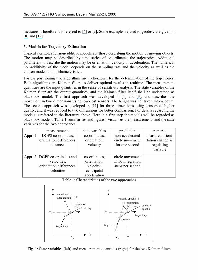
For car positioning two algorithms are well-known for the determination of the trajectories. Both algorithms are Kalman filters to deliver optimal results in realtime. The measurement quantities are the input quantities in the sense of sensitivity analysis. The state variables of the Kalman filter are the output quantities, and the Kalman filter itself shall be understood as black-box model. The first approach was developed in [1] and [3], and describes the movement in two dimensions using low-cost sensors. The height was not taken into account. The second approach was developed in [11] for three dimensions using sensors of higher quality, and it was reduced to two dimensions for better comparison. For details regarding the models is referred to the literature above. Here in a first step the models will be regarded as black-box models. Table 1 summarises and figure 1 visualises the measurements and the state variables for the two approaches.

measurements state variables prediction remarks Appr. 1 DGPS co-ordinates,

orientation differences, distances

co-ordinates, orientation,

velocity

non-accelerated circle movement for one second

measured orient-tation change as

regulating variable

Appr. 2 DGPS co-ordinates and velocities,

orientation differences, velocities

co-ordinates, orientation,

velocity, centripetal

acceleration

circle movement in 50 integration steps per second

Table 1: Characteristics of the two approaches

X

Y

velocity

centripetal acceleration

orientation

|| X

Xi

Yi

trajectory

X

Y

Xi

Yi

trajectory

orientationdifference velocity

epoch i

velocity epoch i- 1

Xi-1

Yi-1

distance

Fig. 1: State variables (left) and measurement quantities (right) for the two Kalman filters

3rd IAG / 12th FIG Symposium, Baden, May 22-24, 2006

The characteristic standard deviations given in table 2 and assumed normal distributions are the base for the simulations in chapter 4. The standard deviations are chosen according to the literature for approach 1 [4] and in appropriate relation for approach 2.

Approach 1 Approach 2 measurement sensor standard deviation measurement sensor standard dev. co-ordinates distances (d)

orientation differences

DGPS Odometer

OSDS Odometer

Gyro

2 m 0,0028 * d [m] 0,001 * d [m]

0,22 [gon/m]* d [m]0,33 gon

co-ordinates velocities (v)

orientation differences

DGPS DGPS OSDS IMS

2 m 0,28 m / s

0,002 * v [m/s]0,17 gon

Table 2 : Simulated stochastic model of the approaches; with: OSDS = optical speed and distance sensor, IMS = Inertial Measurement System

4. Variance-based Sensitivity Analysis for Trajectory Estimation

4.1. Comparison of Models

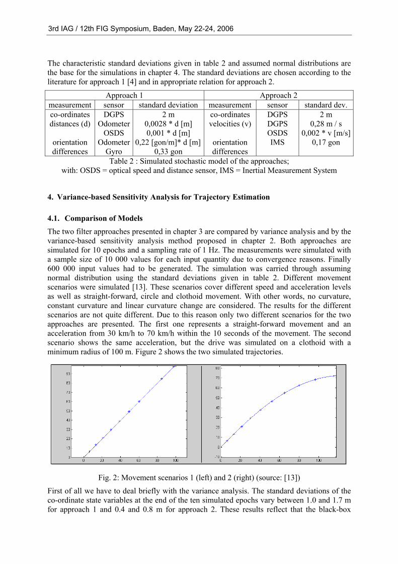
The two filter approaches presented in chapter 3 are compared by variance analysis and by the variance-based sensitivity analysis method proposed in chapter 2. Both approaches are simulated for 10 epochs and a sampling rate of 1 Hz. The measurements were simulated with a sample size of 10 000 values for each input quantity due to convergence reasons. Finally 600 000 input values had to be generated. The simulation was carried through assuming normal distribution using the standard deviations given in table 2. Different movement scenarios were simulated [13]. These scenarios cover different speed and acceleration levels as well as straight-forward, circle and clothoid movement. With other words, no curvature, constant curvature and linear curvature change are considered. The results for the different scenarios are not quite different. Due to this reason only two different scenarios for the two approaches are presented. The first one represents a straight-forward movement and an acceleration from 30 km/h to 70 km/h within the 10 seconds of the movement. The second scenario shows the same acceleration, but the drive was simulated on a clothoid with a minimum radius of 100 m. Figure 2 shows the two simulated trajectories.

Fig. 2: Movement scenarios 1 (left) and 2 (right) (source: [13])

First of all we have to deal briefly with the variance analysis. The standard deviations of the co-ordinate state variables at the end of the ten simulated epochs vary between 1.0 and 1.7 m for approach 1 and 0.4 and 0.8 m for approach 2. These results reflect that the black-box

3rd IAG / 12th FIG Symposium, Baden, May 22-24, 2006

approach 2 delivers more accurate results due to a more sophisticated functional and stochastic model.

For the sensitivity analysis the influences of the measurements of each type e.g. the influences of the DGPS-measured Y co-ordinates were summarised for the ten epochs in groups. Figures 3 to 6 show the total effects estimated by the FAST method of the input quantity groups for the output quantity and state variable, the co-ordinate Y: Y 1 for epoch 1, Y 2 for epoch 2, and so on. For the figures the following abbreviations are valid:

• Y-GPS, X-GPS DGPS co-ordinates • vY-GPS, vX-GPS DGPS velocities • ds-ODSDS distances of optical speed and distance sensor • v-ODSDS velocities of optical speed and distance sensor • ds-Odom distances of odometer • da-Odom, da-Gyro orientation differences of odometer resp. gyroscope • da-INS orientation differences of inertial measurement system

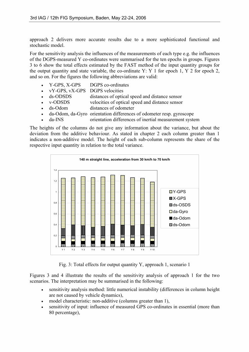
The heights of the columns do not give any information about the variance, but about the deviation from the additive behaviour. As stated in chapter 2 each column greater than 1 indicates a non-additive model. The height of each sub-column represents the share of the respective input quantity in relation to the total variance.

140 m straight line, acceleration from 30 km/h to 70 km/h

0

0,2

0,4

0,6

0,8

1

1,2

1,4

Y 1 Y 2 Y 3 Y 4 Y 5 Y 6 Y 7 Y 8 Y 9 Y 10

Y-GPSX-GPS ds-OSDSda-Gyroda-Odomds-Odom

Fig. 3: Total effects for output quantity Y, approach 1, scenario 1

Figures 3 and 4 illustrate the results of the sensitivity analysis of approach 1 for the two scenarios. The interpretation may be summarised in the following:

• sensitivity analysis method: little numerical instability (differences in column height are not caused by vehicle dynamics),

• model characteristic: non-additive (columns greater than 1), • sensitivity of input: influence of measured GPS co-ordinates in essential (more than

80 percentage),

3rd IAG / 12th FIG Symposium, Baden, May 22-24, 2006

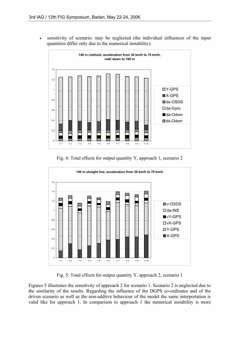
• sensitivity of scenario: may be neglected (the individual influences of the input quantities differ only due to the numerical instability).

140 m clothoid, acceleration from 30 km/h to 70 km/h, radii down to 100 m

0

0,2

0,4

0,6

0,8

1

1,2

1,4

Y 1 Y 2 Y 3 Y 4 Y 5 Y 6 Y 7 Y 8 Y 9 Y 10

Y-GPSX-GPS ds-OSDSda-Gyroda-Odomds-Odom

Fig. 4: Total effects for output quantity Y, approach 1, scenario 2

140 m straight line, acceleration from 30 km/h to 70 km/h

0

0,2

0,4

0,6

0,8

1

1,2

1,4

1,6

Y 1 Y 2 Y 3 Y 4 Y 5 Y 6 Y 7 Y 8 Y 9 Y 10

v-OSDSda-INS vY-GPS vX-GPS Y-GPS X-GPS

Fig. 5: Total effects for output quantity Y, approach 2, scenario 1

Figures 5 illustrates the sensitivity of approach 2 for scenario 1. Scenario 2 is neglected due to the similarity of the results. Regarding the influence of the DGPS co-ordinates and of the driven scenario as well as the non-additve behaviour of the model the same interpretation is valid like for approach 1. In comparison to approach 1 the numerical instability is more

3rd IAG / 12th FIG Symposium, Baden, May 22-24, 2006

obvious. The reason for these instabilities is not clear up to now and demands for further research.

Summarising the simulations the obvious result is that only more accurate GPS measurements would reduce the variances of the state variables. The use e.g. of high-quality gyroscopes would not lead to a reduction of the variance, because their share of the total variance is not essential as shown in the foregoing figures.

4.2. Optimisation of Stochastic Model

Up to now the two approaches were treated as black-box models. To optimise the models one has to know the model and to intervene. A look into the models reflects, that the stochastic models do not coincide with the simulated standard deviations. Especially the DGPS co-ordinates accuracy was modelled too optimistic within the Kalman filter algorithms. Due to these differences the stochastic models were adapted to the realistic simulated variances and the movement scenarios were repeated.

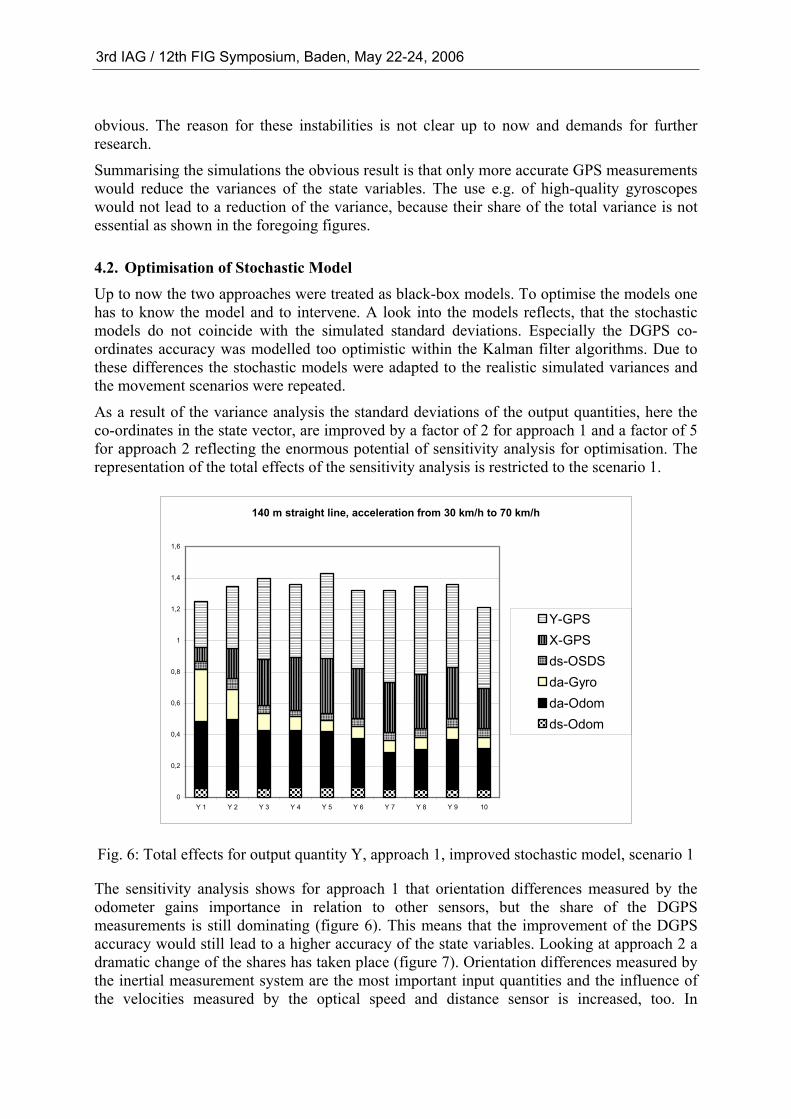
As a result of the variance analysis the standard deviations of the output quantities, here the co-ordinates in the state vector, are improved by a factor of 2 for approach 1 and a factor of 5 for approach 2 reflecting the enormous potential of sensitivity analysis for optimisation. The representation of the total effects of the sensitivity analysis is restricted to the scenario 1.

140 m straight line, acceleration from 30 km/h to 70 km/h

0

0,2

0,4

0,6

0,8

1

1,2

1,4

1,6

Y 1 Y 2 Y 3 Y 4 Y 5 Y 6 Y 7 Y 8 Y 9 10

Y-GPSX-GPSds-OSDSda-Gyroda-Odomds-Odom

Fig. 6: Total effects for output quantity Y, approach 1, improved stochastic model, scenario 1

The sensitivity analysis shows for approach 1 that orientation differences measured by the odometer gains importance in relation to other sensors, but the share of the DGPS measurements is still dominating (figure 6). This means that the improvement of the DGPS accuracy would still lead to a higher accuracy of the state variables. Looking at approach 2 a dramatic change of the shares has taken place (figure 7). Orientation differences measured by the inertial measurement system are the most important input quantities and the influence of the velocities measured by the optical speed and distance sensor is increased, too. In

3rd IAG / 12th FIG Symposium, Baden, May 22-24, 2006

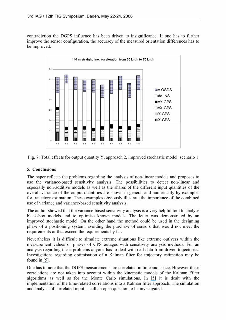
contradiction the DGPS influence has been driven to insignificance. If one has to further improve the sensor configuration, the accuracy of the measured orientation differences has to be improved.

140 m straight line, acceleration from 30 km/h to 70 km/h

0

0,2

0,4

0,6

0,8

1

1,2

1,4

Y 1 Y 2 Y 3 Y 4 Y 5 Y 6 Y 7 Y 8 Y 9 Y 10

v-OSDSda-INSvY-GPSvX-GPSY-GPSX-GPS

Fig. 7: Total effects for output quantity Y, approach 2, improved stochastic model, scenario 1

5. Conclusions The paper reflects the problems regarding the analysis of non-linear models and proposes to use the variance-based sensitivity analysis. The possibilities to detect non-linear and especially non-additive models as well as the shares of the different input quantities of the overall variance of the output quantities are shown in general and numerically by examples for trajectory estimation. These examples obviously illustrate the importance of the combined use of variance and variance-based sensitivity analysis.

The author showed that the variance-based sensitivity analysis is a very helpful tool to analyse black-box models and to optimise known models. The letter was demonstrated by an improved stochastic model. On the other hand the method could be used in the designing phase of a positioning system, avoiding the purchase of sensors that would not meet the requirements or that exceed the requirements by far.

Nevertheless it is difficult to simulate extreme situations like extreme outlyers within the measurement values or phases of GPS outages with sensitivity analysis methods. For an analysis regarding these problems anyone has to deal with real data from driven trajectories. Investigations regarding optimisation of a Kalman filter for trajectory estimation may be found in [5].

One has to note that the DGPS measurements are correlated in time and space. However these correlations are not taken into account within the kinematic models of the Kalman Filter algorithms as well as for the Monte Carlo simulations. In [5] it is dealt with the implementation of the time-related correlations into a Kalman filter approach. The simulation and analysis of correlated input is still an open question to be investigated.

3rd IAG / 12th FIG Symposium, Baden, May 22-24, 2006

References: [1] Aussems, T.: Positionsschätzung von Landfahrzeugen mittels KALMAN-Filterung aus

Satelliten- und Koppelnavigationsbeobachtungen. Veröffentlichungen des Geodätischen Instituts der Rheinisch-Westfälischen Technischen Hochschule Aachen, Nr. 55, 1999.

[2] Cukier, R. I., Fortuin, C. M., Shuler, K. E., Petschek, A. G., Schaibly, J. H.: Study of the sensitivity of coupled reaction systems to uncertainties in rate coefficients. Part I: theory. Journal of Chemical Physics, Vol. 59, No. 8, 1973.

[3] Eichhorn, A.: Ein Beitrag zur Identifikation von dynamischen Strukturmodellen mit Methoden der adaptiven KALMAN-Filterung. Deutsche Geodätische Kommission, Reihe C, Heft 585, 2005.

[4] Ramm, K., Schwieger, V.: Multisensorortung für Kraftfahrzeuge. In: Schwieger, V., Foppe, K. (Ed., 2004): Kinematische Messmethoden – Vermessung in Bewegung, DVW Schriftenreihe, Band 45, Wißner Verlag, Augsburg, 2004.

[5] Ramm, K.: Enhanced Kinematic Positioning Methods by Shaping Filter Augmentation. Proceedings on 3rd IAG Symposium on Structural Engineering, Baden, Austria, 22nd – 24th May 2006.

[6] Saltelli, A., Chan, K., Scott, E.M. (Ed.): Sensitivity Analysis. John Wiley and Sons, Chichester, 2000.

[7] Saltelli, A., Tarantola, S., Campolongo, F., Ratto, M.: Sensitivity Analysis in Practise. John Wiley and Sons, Chichester, 2004.

[8] Schwieger, V.: Variance-based Sensitivity Analysis for Model Evaluation in Engineering Surveys. Proceedings on 3rd International Conference on Engineering Surveying, Bratislava, Slovakia, 11th-13th November 2004.

[9] Schwieger, V.: Nicht-lineare Sensitivitätsanalyse, gezeigt an Beispielen zu bewegten Objekten. Deutsche Geodätische Kommission, Reihe C, No. 531, 2005.

[10] Sobol, I. M.: Sensitivity Estimates for Nonlinear Mathematical Models. Mathematical Modelling and Computational Experiments, Volume 1(4), 1993.

[11] Sternberg, H.: Zur Bestimmung der Trajektorie von Landfahrzeugen mit einem hybriden Messsystem. Schriftenreihe des Studiengangs Geodäsie und Geoinformatik an der Universität der Bundeswehs Neubiberg, No. 67, 2000.

[12] Tiede, C., Tiampo, K., Fernandez, J., Gerstenecker, C.: Deeper understanding of non-linear geodetic data inversion using quantitative sensitivity analysis. Nonlinear Processes in Geophysics, 12, pp 373-379, 2005.

[13] Wilhelm, D.: Ein Beitrag zur Validierung zweier Modellierungsansätze für bewegte Fahrzeuge unter Nutzung der varianz-basierten Sensitivitätsanalyse. Study Thesis at IAGB, Universität Stuttgart, 2005 (unpublished).

3rd IAG / 12th FIG Symposium, Baden, May 22-24, 2006