Self-optimizing adaptive optics control with Reinforcement Learningfor high-contrast imaging

Rico Landmana,*, Sebastiaan Y. Hafferta,b,c, Vikram M. Radhakrishnana, Christoph U.Kellera

aLeiden Observatory, Leiden University, PO Box 9513, 2300 RA Leiden, The NetherlandsbSteward Observatory, Unversity of Arizona, 933 North Cherry Avenue, Tucson, ArizonacNASA Hubble Fellow

Abstract. Current and future high-contrast imaging instruments require extreme adaptive optics (XAO) systemsto reach contrasts necessary to directly image exoplanets. Telescope vibrations and the temporal error induced bythe latency of the control loop limit the performance of these systems. One way to reduce these effects is to usepredictive control. We describe how model-free Reinforcement Learning can be used to optimize a Recurrent NeuralNetwork controller for closed-loop predictive control. First, we verify our proposed approach for tip-tilt control insimulations and a lab setup. The results show that this algorithm can effectively learn to mitigate vibrations andreduce the residuals for power-law input turbulence as compared to an optimal gain integrator. We also show thatthe controller can learn to minimize random vibrations without requiring online updating of the control law. Next,we show in simulations that our algorithm can also be applied to the control of a high-order deformable mirror. Wedemonstrate that our controller can provide two orders of magnitude improvement in contrast at small separationsunder stationary turbulence. Furthermore, we show more than an order of magnitude improvement in contrast fordifferent wind velocities and directions without requiring online updating of the control law.

Keywords: Adaptive Optics, Predictive Control, High Contrast Imaging, Reinforcement Learning, Machine Learning.

*Rico Landman, rlandman@strw.leidenuniv.nl

1 Introduction

One of the main limitations of current and future ground-based high contrast imaging (HCI) in-struments is the wavefront error induced by the time lag between sensing and correcting the wave-front.1 This time lag results in a halo of speckles along the wind direction, which limits the contrastat small separations.2 Furthermore, the finite control bandwidth results in low-order residuals afterthe correction, such as tip and tilt. One of the main causes of these residuals are vibrations close tothe maximum control frequency. All ground-based high-contrast imaging instruments suffer fromvibrations, including SCExAO,3 GPI4 and SPHERE.5 These vibrations decrease the resolution oflong-exposure images. Furthermore, some coronagraphs are highly sensitive to residual tip-tilt,6, 7

which will further reduce the contrast.Both of these effects can be reduced with better control algorithms. Early work on improved

controllers involved optimizing the modal gains of a modal integrator based on the open-looptemporal Power Spectral Density (PSD).8, 9 This optimal gain is a trade-off between turbulencerejection and the amplification of noise and disturbances outside the control bandwidth. However,to reduce the effect of the servo-lag we have to predict the disturbances before they are measured.A popular approach to optimal control is Linear Quadratic Gaussian (LQG) control,10 which isbased on a Kalman filter. Variants of LQG-based controllers have been demonstrated to reducetip-tilt vibrations in simulations,11 lab verifications12 and on-sky.4, 13, 14 A disadvantage of LQG-like controllers is their reliance on a linear state-space model of the turbulence and deformable

1

arX

iv:2

108.

1133

2v1

[as

tro-

ph.I

M]

24

Aug

202

1

mirror (DM) dynamics;15 this requires accurate calibration of the model parameters. Hence, thesecontrollers can also not correct for correlations in the turbulence that are not included in the model.A combination of an LQG controller for low-order vibrations and an optimal modal gain inte-grator for high-order modes is currently being used in the adaptive optics (AO) systems of bothSPHERE14 and GPI.16

Another group of data-driven algorithms construct a linear filter that minimizes the residualphase variance from (pseudo) open-loop data. This idea was originally proposed and demon-strated for modal control by Dessenne et al.17 More recently, a spatio-temporal filter based onEmpirical Orthogonal Functions (EOFs) was demonstrated to significantly increase the contrastin a simulated HCI system.18 The performance of such linear filters was tested on open-loop AOtelemetry for the Keck II AO system19 and SPHERE20 and showed a decrease in residual wave-front error. An issue with these data-driven predictive control algorithms is that they rely on theprediction of (pseudo) open-loop wavefront data, while XAO systems operate in closed-loop. Touse these controllers, one has to reconstruct the pseudo open-loop residuals. Not only does thisrequire knowledge of the servo-lag of the system and DM dynamics, it is also not trivial in thecase where the response of the wavefront sensor is nonlinear, such as for the Pyramid Wavefrontsensor.21 To circumvent the issue of nonlinearity, neural networks can improve the performancecompared to linear models when using an unmodulated Pyramid Wavefront Sensor.22 However,predicting the open-loop residuals alone does not provide the optimal closed-loop control law. Forexample, one still has to find the best gain for the control loop. Furthermore, as the open-loopwavefront may be orders of magnitude larger than the closed-loop errors, a relative error in thepredicted open-loop wavefront may be detrimental to the closed-loop contrast as compared witha relative error in the closed-loop residuals. Obtaining a closed-loop control law using supervisedlearning approaches is hampered by the distribution of inputs depending on the control law itself.It was recently shown that this can be mitigated by using an adversarial prior in the training of aneural-network controller.23 Instead of predicting in open-loop while controlling in closed-loop,we can also do data-driven predictive control directly in closed-loop. This can for example bedone using data-driven subspace predictive control, which was recently shown to provide ordersof magnitude improvement in contrast in simulations and in the lab.24 This does not require theexplicit prediction of the wavefront after a known servo-lag but directly optimizes the closed-loopcommands. The proposed approach here is similar, but generalizes to nonlinear control laws andarbitrary optimization objectives.

Another issue for most of these approaches is the non-stationary nature of turbulence.25 Allmethods mentioned above require online updating of the control parameters based on the currentturbulence parameters. This updating of the control law is computationally very expensive andoften involves inverting large matrices.18, 26 Recently, it was shown that a single Artificial NeuralNetwork (ANN) can learn to predict the open-loop wavefront for varying wind speeds and direc-tions for a simulated AO system.27 This eliminates the need for updating the control law to keep upwith changing turbulence properties. This would allow us to decouple the training of the controllerfrom online control, simplifying the implementation and potentially gaining in stability. However,using this approach still leaves the problems associated with predicting the open-loop turbulence.

Here, we use Reinforcement Learning (RL), a Machine Learning approach, for the data-drivenoptimization of the closed-loop adaptive optics control law. Indeed, Machine Learning has re-cently received significant attention in the AO community for wavefront reconstruction,28, 29 pre-diction27, 30 and control;22, 23 Reinforcement Learning was already suggested as a method to directly

2

optimize the contrast in a high-contrast imaging system31 and for focal-plane wavefront control.32

Very recently, model-based RL was proposed for adaptive optics control,33 and was shown toreduce the temporal error and adjust to mis-registrations between the deformable mirror and wave-front sensor. Our proposed approach here has similar advantages as their approach. The maindifference is the use of a parameterized control law here over a planning algorithm. This avoidsthe need for solving the planning optimization for every control command, which is generallytoo computationally expensive to do at kHz frequencies, at which typical XAO systems are run.However, this generally comes at the cost of longer training times.

Our RL-based approach has some distinct advantages:

• Data-driven: The algorithm is completely self-optimizing and data-driven; it does not re-quire an explicit model of the disturbances or system dynamics, or knowledge of systemparameters. Instead of explicitly predicting the wavefront after an assumed servo-lag, itdirectly optimizes the closed-loop commands.

• Flexible: The algorithm allows for an arbitrary optimization objective. The user is free tochoose the metric to optimize based on the science goals of the instrument. Furthermore, itcan handle multiple inputs including systems with multiple wavefront sensors.

• Nonlinear: The proposed method can optimize any parameterized, differentiable controllaw. For example, one can optimize the parameters of a nonlinear Artificial Neural Network(ANN) controller. This allows the controller to model the nonlinear dynamics of the system,such as for systems with a Pyramid Wavefront Sensor. Because of the larger representationpower of these Neural Networks, they can also learn to perform under varying atmosphericconditions.

This paper is structured as follows: Section 2 provides an introduction to Reinforcement Learningand describes the relevant algorithm. Section 3 simulates the algorithm’s performance in tip-tiltcontrol for vibrations and a power-law input, while section 4 shows the results from a lab experi-ment. Section 5 shows the results of using the algorithm to control a high-order deformable mirror.Finally, section 6 draws conclusions and outlines future work.

2 Reinforcement Learning Control

We begin the description of our algorithm with an introduction to the Reinforcement Learningframework, within which we formulate the AO control problem. This is followed by a discussion ofthe Deterministic Policy Gradient algorithm and how it can be applied to closed-loop AO control.

2.1 AO control as a Markov Decision Process

Reinforcement Learning34 (RL) algorithms deal with Markov Decision Processes (MDPs), discrete-time stochastic control processes. In the RL framework, an agent operates within an environment,which is formally defined by a tuple (S,A,R,P) and time index t. Here, st ∈ S is the state of theenvironment, at ∈ A the action taken by the agent,R the reward function and P the state transitionprobabilities defined by:

P(st, at, st+1) = P (st+1|st, at), (1)

3

Table 1 Overview and explanation of the various terms used in the Reinforcement Learning (RL) framework.

Symbol RL term AO term/Explanations State Input to the controller.o Observation Measurement of the residual wavefronta Action Incremental DM commandsr Reward Measure of the instantaneous performance; we are free to choose thisR Return Discounted sum of future rewards; the optimization objectiveπθ Actor/policy The control lawQω Critic Estimate of the return/the cost function

where P (st+1|st, at) gives the probability of transitioning from state st to state st+1 as a result ofaction at. The state needs to be defined in such a way that the transition probabilities are fullydescribed by Eq. 1 and do not depend on previous states (e.g. st−1). This is also known as theMarkov property.

In the case of AO control, the agent is the DM controller. The environment consists of every-thing but the controller, including the evolution of the turbulence and the DM dynamics. At eachtime step the the controller receives a state st. For example, in the case of an integral controller thestate consists of only the most recent observation of the residual wavefront ot. The representationof the state for our Reinforcement Learning controller will be extensively discussed in section 2.4.Based on this state, the controller takes an action at, following some control law π: at = π(st).Since the controller operates in closed loop, this action consists of the incremental voltages addedto the DM, equivalent to an integral controller. The DM commands and the temporal evolution ofthe environment result in the transition to a new state st+1, according to the transition probabilitiesP of the stochastic process of the turbulence, and a reward rt = R(st, at, st+1). This reward is ameasure of the performance of the controller; the reward function R can be arbitrarily chosen aslong as it can be calculated at every time step. The goal is to determine the control law π that givesthe highest cumulative future reward. To ensure that the cumulative future reward remains finiteand to prioritize immediate rewards, future rewards are discounted at a rate γ < 1, the discountfactor. The discounted future return Rt is then defined as:

Rt =∑t=0

γtrt = rt + γrt+1 + γ2rt+2 + . . . . (2)

The optimization objective can then be formally defined as:

J(π) = Es∼ρπ ,a∼π[R]. (3)

Here, E denotes the expectation value and ρπ the state visitation distribution when following thecontrol law π. This state visitation distribution describes how often we end up in state s if wefollow the control law π. This expectation over the state visitation distribution is taken because wewant to optimize over the states that we observe. It also accounts for the dependency of the inputson the controller. In the rest of this work, when we denote an expectation value, it is always overs ∼ ρπ and a ∼ π, and we will leave this out for readability. There are a variety of algorithms tofind an optimal control law in the above framework.35 One of the most frequently used algorithmsfor continuous control problems is the (Deep) Deterministic Policy Gradient algorithm,36, 37 which

4

we will use here. Our choice for the DDPG algorithm was motivated by the need for a directlyparameterized and deterministic control law, which allows for the fast computation of the DMcommands at kHz frequencies without needing to solve a planning optimization problem everymillisecond. Furthermore, while not explored in this work, we preferred an algorithm which allowsfor an arbitrary optimization objective and could therefore also be used for the direct optimizationof a focal plane quantity, such as the Strehl ratio or the post-coronagraphic contrast. Finally, sinceit is generally easy to collect a lot of data, as we generate 1000 datapoints per second at 1 kHz, thelower sample efficiency of model-free1 algorithms was considered less of an issue.

2.2 (Deep) Deterministic Policy Gradient

The (Deep) Deterministic Policy Gradient (DPG)36 algorithm uses two parameterized models:

• An Actor πθ(s) that models the control law with parameters θ. This model maps the state tothe DM commands : at = πθ(st).

• A Critic Qω(s, a) that models the expected return for a given state and DM command withparameters ω: Qω(st, at) = E[Rt|st, at]. This is an estimation of the cost function that hasto be optimized.

Both the actor and critic may be any kind of parameterized, differentiable model. These mayfor example be function approximators, such as Artificial Neural Networks (ANN).38 The DPGalgorithm with ANNs as function approximators is referred to as the Deep Deterministic PolicyGradient (DDPG) algorithm.37 In this case, θ and ω are the trainable parameters of the ANN forthe actor and critic, respectively. The algorithm aims to find the parameters θ of the controller thatmaximizes the optimization objective J(πθ). Using the actor and the critic we can calculate thegradients of the optimization objective with respect to the control parameters using the chain rule:

∇θJ(πθ) =E[∇θQω(s, a)]

=E[∇aQω(s, a)∇θπθ(s)](4)

These gradients can then be used by a gradient-based optimizer to update the parameters θ of thecontrol law in the direction in which the expected return increases. The quality of the controllerthus inherently depends on the ability of the critic Qω(s, a) to successfully model the expectedreturn. The critic can be taught using Temporal Difference (TD) learning, which uses the Bellmanequation39 to bootstrap the expected future reward:

Qω(st, at) =E[Rt|st, at]=E[rt + γrt+1 + γ2rt+2 + . . . ]

=E[rt + γ(rt+1 + γrt+2 + . . . )]

=E[rt + γQω(st+1, π(st+1))] ≡ E[yt],

(5)

where yt are referred to as the target values and are calculated using:

yt = rt + γQω(st+1, π(st+1)). (6)1Model-free in the RL context does not imply that we do not have an empirical model for the controller. Instead,

it means that the algorithm does not explicitly model the transition dynamics and plans through this model to find theoptimal commands/policy.

5

Training the critic can then be framed into a supervised learning problem for each iteration, wherewe try to find the parameters ω that minimize the mean-squared error between the output of thecritic and the target values yt. The critic loss L is thus given by:

L(ω) = −1

2E[(yt −Qω(st, at))

2], (7)

and its gradients with respect to the parameters ω by:

∇ωL(ω) = −E[(yt −Qω(st, at))∇ωQω(st, at)]. (8)

We can then use a gradient-based optimizer to update the parameters in the direction that minimizesthe loss. However, since the target values depend on the critic itself, this may quickly lead toinstabilities in the training process. It is therefore common to use target models Q′ and π′ tocalculate the target values yt.37 The parameters of these target models slightly lag behind the truemodels. For every iteration i of training the critic, the target models are updated as:

θ′i = τθi + (1− τ)θ′i−1ω′i = τωi + (1− τ)ω′i−1.

(9)

Here, τ < 1 is a hyper-parameter that determines how quickly the target models are updated.

2.3 Data collection

Updating the actor and critic requires evaluating expectation values over the state visitation distri-bution. This can naturally be done by collecting tuples (st, at, rt st+1) while following the controllaw πθ. For our purpose, this is done by running the AO system in closed-loop with the controllerπθ. This data collection process is often separated into episodes of finite length, after which thesequence of tuples is saved in a so-called replay buffer, which is our training data set. For compu-tational reasons, the expectation values are often estimated over a limited number of these tuples, abatch, instead of over the full data set. To reduce the correlation in a batch, the tuples are randomlysampled from the replay buffer.

The DDPG algorithm is off-policy,36, 37 meaning that it is not strictly required to sample thetraining data with the current policy. In principle, we can use any other controller, or even randomactions, to generate the training tuples of states, actions and rewards. While this introduces amismatch between the distribution of the training data and the true state visitation distribution ofthe current controller, this is often ignored in practice. Therefore, we can use previously collecteddata, where the control law was different, to train the controller. Furthermore, it is also possible toinclude data from a completely different controller, such as an integrator, to train the RL controller.This way, the algorithm could also make use of historically collected telemetry data using thecurrent controller at the telescope.

Because the algorithm allows for the data collection to be done with a different controller, wecan also add some known disturbances to the commands. This is called exploration in the RLframework. For example, we can add some zero mean, normally distributed exploration noise withstandard deviation σ:

at = πθ(st) +N (0, σ) (10)

6

This results in the controller not always giving the same DM commands for a given state, suchthat we can observe the results of these different commands. A common trick is to use large initialexploration noise and slowly decay it. This allows the algorithm to first observe the results of largechanges in DM commands and finally observe the result of small changes in these commands. Weempirically choose the standard deviation of the exploration noise during episode k as:

σk =σ0

1 + ζkrad. (11)

Here, σ0 is a hyper-parameter that specifies the initial standard deviation of the exploration noiseand ζ how quickly it decays.

2.4 State representation

It is crucial to have a representation of the state st such that the problem obeys the Markov prop-erty (Eq. 1), which requires that the state-transition probabilities are fully described by the currentstate and the action taken. This is not trivial in closed-loop AO control. A first guess for the statemight be the most recent wavefront observation, ot. This may, for example, be retrieved from adedicated wavefront sensor (WFS). However, defining the state like this is not consistent with theMarkov property. First of all, we do not have access to the full state of the environment but onlyobserve a noisy representation with the WFS measurements. Furthermore, the most recent wave-front measurement does not contain all the required information; for example, it lacks informationabout possible vibrations and wind flow. When the AO loop is closed, we also have to distinguishchanges in the turbulence profile from changes due to previous commands, as we only observe theclosed-loop residuals. These issues may be solved using state augmentation, where sequences ofprevious wavefront measurements and applied DM commands are used in the state. However, if wewant our controller to be able to perform under varying conditions, it may require a large numberof previous measurements to have a full representation of the state. For example, Guyon & Males18

used a vector of the previous 800 measurements to correct tip-tilt vibrations. A disadvantage ofthis is that it increases the computational demand. Furthermore, all previous measurements arein principle weighted equally, which may lead to additional noise if the problem is not correctlyregularized.

To circumvent the problem of partial observability, it was shown that Recurrent Neural Net-works (RNNs) are able to solve control problems even for partially observable Markov DecisionProcesses, where the Markov property is not obeyed.40, 41 RNNs are a type of neural network oftenused in processing sequential data.38, 42 Instead of only mapping an input to an output, RNNs alsoupdate a memory state mt based on the previous memory state and the input. This allows RNNs tosummarize previous information in this memory state and use it to calculate the output. This en-ables RNNs to learn an internal representation of the true state of the system based on sequences ofnoisy measurements. As an additional advantage calculating the control commands only requiresthe most recent observation to be propagated through the controller. This is computationally lessdemanding, which may be important for high-order AO systems operating at kHz frequencies.Furthermore, RNNs also effectively use the temporal structure of the data by incorporating basicpriors, such as that the most recent measurement is the most relevant instead of using one largevector of components with equal weights. In our case, we will use a Long Short-Term Memory(LSTM) cell43 as the recurrent architecture. Training is now done on sequences of states, actions

7

and rewards using Truncated Backpropagation Trough Time (TBTT) over a length l. This versionof the algorithm is known as the Recurrent Deterministic Policy Gradient (RDPG) algorithm.41

The state for closed-loop AO now consists of only the most recent observation of the wavefrontot and the previous DM commands at−1:

st = (ot, at−1) . (12)

2.5 Algorithm Overview

The algorithm can be summarized in three main steps that are iteratively performed:

1. Collect training sequences (o1, a1, r1, . . . ot, at, rt) by running in closed loop and storing thedata in the replay buffer.

2. Train the critic using Temporal Difference learning on the observed data.

3. Improve the control law using the gradients obtained from the critic.

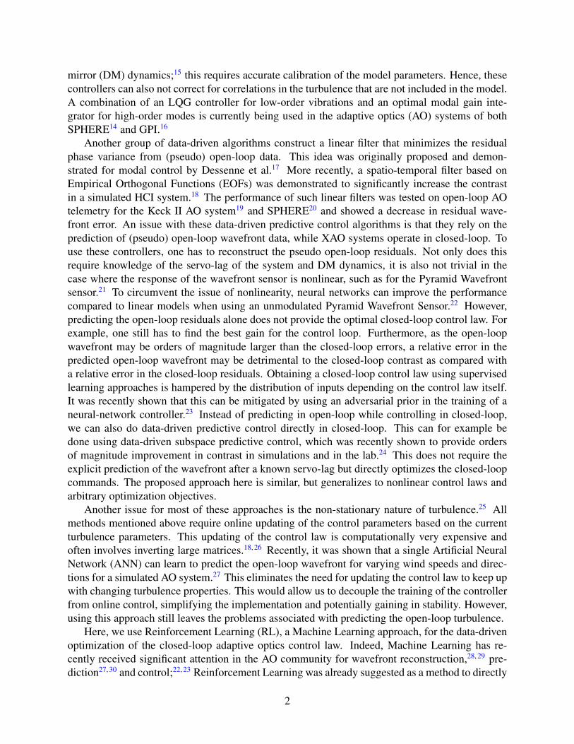
The pseudo-code describing the full algorithm can be found in Algorithm 1, and a schematicoverview is shown in Fig 1.

Fig 1 Visual overview of the algorithm. The black line indicates forward propagation. The green and red lines indicatehow we backpropagate the gradients to update the critic and the actor, respectively.

8

Algorithm 1: Recurrent Deterministic Policy Gradient for closed-loop AO (based onHeess et al.41)

Initialize critic parameters ω and actor parameters θ randomlyInitialize target network parameters ω′ = ω, θ′ = θInitialize replay bufferInitialize σ0 and ζfor k=1,number of episodes do

Reset controller memory states mt = 0 and deformable mirrorfor t=1,T do

Receive wavefront measurement ot, reward rt, construct state st = (ot, at−1) andselect incremental DM commands at = π(st) + ε, with ε ∼ N (0, σk)

endSave trajectories (o1, a1, r1, . . . , oT , aT , rT ) in replay bufferDecay exploration noise σk = σ0

1+ζk

for j=1,number of training steps doRandomly sample N batches of length l from the replay bufferFor each batch i construct state histories hit = ((oi1, a

i0) . . . , (o

it, a

it−1))

Calculate the critic targets using the Bellman equation:

yit = rit + γQ′ω′(hit+1, π′θ′(h

it+1))

Calculate the sampled critic loss gradient with TBTT:

∇ωL(ω) ≈1

Nl

N∑i=1

l∑t=1

(yit −Qω(hit, a

it))∇ωQω(s

it, a

it)

Calculate the sampled Policy Gradient with TBTT:

∇θJ(θ) ≈1

Nl

N∑i

l∑t

∇aQω(hit, a

it)∇θπθ(h

it)

Use a gradient-based optimizer (e.g. Adam) to update the actor parameters θ andcritic parameters ω.

Update the target network parameters:

θ′j = τθj + (1− τ)θ′j−1ω′j = τωj + (1− τ)ω′j−1

endend

9

3 Tip-tilt control in simulations

3.1 Simulation setup

As a proof of concept we apply the algorithm to tip-tilt control in simulations. We simulate anidealized optical system using the HCIPy44 package for python. Our system has an unobscured,circular aperture of 1 meter in diameter and operates at a wavelength of 1 µm. The simulateddeformable mirror has only two degrees of freedom, its tip and tilt. The observation ot is the centerof gravity (xt, yt) of the focal plane image in units of λ/D. The measured center of gravity alongwith the previous DM commands at−1 are fed into a controller that controls tip and tilt in closedloop. To represent the servo-lag of estimating the wavefront tip and tilt, calculating and applyingthe control commands, we delay the DM commands by a discrete number of frames:

DMt = DMt−1 + at−τ , (13)

where τ is the servo lag. This is equivalent to the controller seeing the state from τ iterationsago, which implies a delay in obtaining the reward. Throughout this section we assume an AOsystem operating at 1 kHz with a servo lag of 3 frames and do not consider any detector noise.Furthermore, we only simulate tip-tilt errors and ignore all higher order modes in the simulations.

3.1.1 Algorithm setup

To minimize the residual tip-tilt jitter we choose the squared deviation of the center of gravity ofthe PSF as the reward function:

rt = −x2t + y2tb2

. (14)

Here, b is a scaling factor for which we use a value of 4λ/D in the simulations. This scaling factoracts as a normalization of the rewards. Here, we empirically choose a value for the scaling factor,but this could also be inferred from the data. Important to note is that this scaling factor also scalesthe gradient of the reward with respect to the DM commands and therefore also influences thegradient update of the actor.

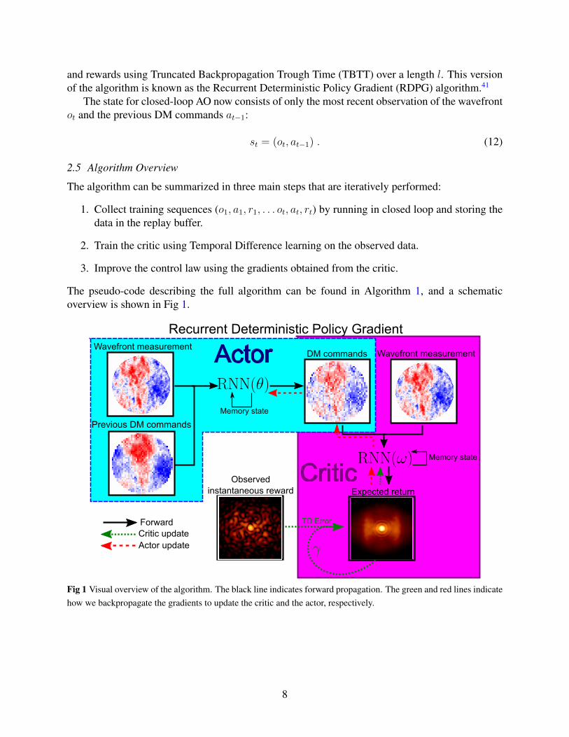
We use the same Neural Network architecture for both the actor and the critic. The input con-sists of the wavefront measurement ot = (xt, yt) and the previously applied tip-tilt commandsat = (ax,t−1, ay,t−1). We use a Long Short-Term Memory43 (LSTM) cell with 64 neurons as therecurrent layer in both the actor and the critic. For the critic the DM commands at are appendedto the output of the LSTM. After that, we have a fully connected layer with 64 neurons for bothnetworks. Finally, the output of the actor consists of two neurons, the additional tip and tilt com-mands, while the output of the critic is a single neuron that estimates the expected future returnQ(st, at). The LSTM uses a tanh activation function for the input and output gates and a hardsigmoid for the recurrent gates while the fully connected layer uses the ReLU activation function.The output of the actor again uses a tanh activation function to constrain the incremental DM com-mands between -1 rad and +1 rad. The output of the critic has a linear activation function. Thearchitectures are also listed in Table 2. Both the actor and critic have ∼ 22, 000 free parameters.This is likely a lot more than required for tip-tilt control. Optimization of the architecture mayresult in shorter training times and improved performance, but is beyond the scope of this work.

We use the gradient-based Adam optimizer algorithm45 with default parameters except for thelearning rate. After every 500 iterations (an episode), we reset the DM shape. To reduce the

10

correlation of the data in a batch early on, we only start training after a certain number of episodes,the warmup. We use a warmup of 5 episodes, which is equivalent to 2500 iterations, and theexploration law given in Eq. 11. The hyperparameters of the RDPG algorithm are given in Table3. The algorithm and Neural Networks are implemented using a combination of the TensorFlow46

version 1.15 and Keras47 packages for Python.

Table 2 Neural Network architectures of the actor and critic for the tip-tilt control.Layer type Neurons Input shape Activation function

Act

or LSTM 64 (4) TanhDense 64 (64) ReLUDense 2 (64) Tanh

Layer type Neurons Input shape Activation function

Cri

tic

LSTM 64 (4) TanhConcatenate - (64) and (2) -Dense 64 (66) ReLUDense 1 (64) Linear

Table 3 HyperparametersParameter Value

Actor learning rate 10−5

Critic learning rate 10−3

Target network soft update τ 10−3

Discount factor γ 0.99Batch size 64

TBTT length l 50 msInitial exploration σ0 0.3 radExploration decay ζ 0.005

Episode length 500 iterationsNumber of training steps per episode 500

3.2 Vibration Suppression

As an example we consider an input disturbance consisting of three pure vibrations along each ofthe x and y directions. Along the x direction we have vibrations with frequencies at 13 Hz, 37Hz and 91 Hz and along the y direction at 11 Hz, 43 Hz and 87 Hz. The gain of the integratoris optimized by running in closed loop for 1 second and choosing the gain that gives the lowestresidual root mean square (RMS) center deviation:

RMS =√< x2t + y2t >. (15)

Figure 2 shows the evolution of the RMS during the training of the RL controller. It shows thatafter a few thousand iterations the RL controller outperforms the integrator and eventually reachesan average RMS that is a factor 6 lower than for the integrator. The figure also shows the tempo-ral PSD of the residuals along the x-direction for the fully trained controller without exploration

11

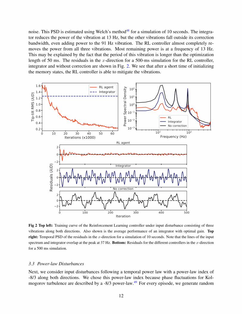
noise. This PSD is estimated using Welch’s method48 for a simulation of 10 seconds. The integra-tor reduces the power of the vibration at 13 Hz, but the other vibrations fall outside its correctionbandwidth, even adding power to the 91 Hz vibration. The RL controller almost completely re-moves the power from all three vibrations. Most remaining power is at a frequency of 13 Hz.This may be explained by the fact that the period of this vibration is longer than the optimizationlength of 50 ms. The residuals in the x-direction for a 500-ms simulation for the RL controller,integrator and without correction are shown in Fig. 2. We see that after a short time of initializingthe memory states, the RL controller is able to mitigate the vibrations.

Fig 2 Top left: Training curve of the Reinforcement Learning controller under input disturbance consisting of threevibrations along both directions. Also shown is the average performance of an integrator with optimal gain. Topright: Temporal PSD of the residuals in the x-direction for a simulation of 10 seconds. Note that the lines of the inputspectrum and integrator overlap at the peak at 37 Hz. Bottom: Residuals for the different controllers in the x-directionfor a 500 ms simulation.

3.3 Power-law Disturbances

Next, we consider input disturbances following a temporal power law with a power-law index of-8/3 along both directions. We chose this power-law index because phase fluctuations for Kol-mogorov turbulence are described by a -8/3 power-law.49 For every episode, we generate random

12

power-law time series for 500 ms, neglecting frequencies below 2 Hz. The training curve is shownin Fig. 3. We again observe better RMS performance for the RL controller as compared to anintegrator with optimized gain. We test the trained controller by running in closed loop for 10s and calculating the temporal PSD of the residuals, which are also shown in Fig. 3. The RLcontroller has a larger rejection power at lower frequencies. The residual PSD of the integratorexhibits a bump around 70 Hz, which is the result of the integrator overshooting. A lower gainwould reduce this overshooting but would also decrease its rejection power at lower frequencies.The RL controller can account for already applied commands that are not yet visible in the residualmeasurements due to the servo lag, allowing it to use a higher gain without overshooting. The RLcontroller adds power at high frequencies. This is the result of the waterbed effect, which impliesthat if we decrease the power at one part of the spectrum this always leads to the amplification ofanother part of the spectrum.

Fig 3 Left: Training curve of the Reinforcement Learning controller under power-law input turbulence and the av-erage performance of an integrator with optimal gain. Right: Temporal PSD of the residuals in the x-direction for asimulation of 10 seconds.

4 Lab verification of tip-tilt control

4.1 Experimental Setup

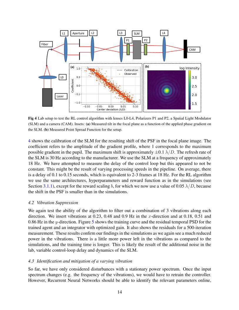
The results in the previous section are based on idealized simulations. To validate our results fortip-tilt control we tested the algorithm in the lab. The lab setup is sketched in Figure 4. The firstlens focuses a 633-nm He-Ne laser onto a single-mode fiber. The fiber output is then collimated,and a diaphragm defines the input aperture. A 4f system reimages the aperture onto a HoloeyeLC2002 Spatial Light Modulator (SLM) with 800x600 pixels. The pupil covers approximately200x200 pixels on the SLM. Right before the SLM we define the polarization with a polarizer.After a second polarizer we focus the beam onto the camera. The resulting Point Spread Functionis shown in Figure 4.

We use the SLM as both the turbulence generator and the corrector. The polarizers are rotatedsuch that the SLM mainly manipulates the phase profile with minimum amplitude modulation.The voltages of the SLM are controlled with 8-bit resolution. As the response for both small andlarge voltages becomes highly nonlinear, only values between 25 and 225 are used. Tip and tiltaberrations are introduced by applying a gradient on the SLM at the location of the pupil. Figure

13

L1 Aperture L2 L3 L4SLM

CAM

P1 P2Fiber

Laser

L0

(a) (b)

Fig 4 Lab setup to test the RL control algorithm with lenses L0-L4, Polarizers P1 and P2, a Spatial Light Modulator(SLM) and a camera (CAM). Insets: (a) Measured tilt in the focal plane as a function of the applied phase gradient onthe SLM. (b) Measured Point Spread Function for the setup.

4 shows the calibration of the SLM for the resulting shift of the PSF in the focal plane image. Thecoefficient refers to the amplitude of the gradient profile, where 1 corresponds to the maximumpossible gradient in the pupil. The maximum shift is approximately±0.1 λ/D. The refresh rate ofthe SLM is 30 Hz according to the manufacturer. We use the SLM at a frequency of approximately18 Hz. We have attempted to measure the delay of the control loop but this appeared to not beconstant. This might be the result of varying processing speeds in the pipeline. On average, thereis a delay of 0.1 to 0.15 seconds, which is equivalent to 2-3 frames at 18 Hz. For the RL algorithmwe use the same architectures, hyperparameters and reward function as in the simulations (seeSection 3.1.1), except for the reward scaling b, for which we now use a value of 0.05 λ/D, becausethe shift in the PSF is smaller than in the simulations.

4.2 Vibration Suppression

We again test the ability of the algorithm to filter out a combination of 3 vibrations along eachdirection. We insert vibrations at 0.23, 0.48 and 0.9 Hz in the x-direction and at 0.18, 0.51 and0.86 Hz in the y-direction. Figure 5 shows the training curve and the residual temporal PSD for thetrained agent and an integrator with optimized gain. It also shows the residuals for a 500-iterationmeasurement. These results confirm our findings in the simulations as we again see a much reducedpower in the vibrations. There is a little more power left in the vibrations as compared to thesimulations, and the training time is longer. This is likely the result of the additional noise in thelab, variable control-loop delay and dynamics of the SLM.

4.3 Identification and mitigation of a varying vibration

So far, we have only considered disturbances with a stationary power spectrum. Once the inputspectrum changes (e.g. the frequency of the vibrations), we would have to retrain the controller.However, Recurrent Neural Networks should be able to identify the relevant parameters online,

14

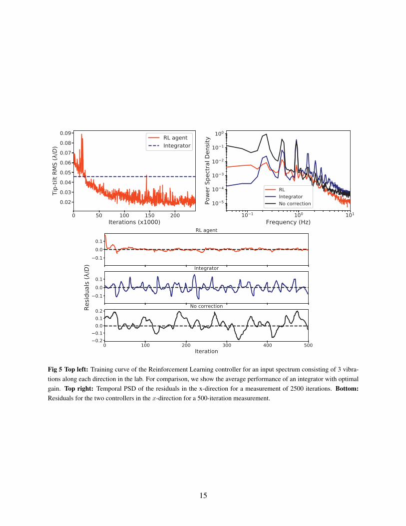
Fig 5 Top left: Training curve of the Reinforcement Learning controller for an input spectrum consisting of 3 vibra-tions along each direction in the lab. For comparison, we show the average performance of an integrator with optimalgain. Top right: Temporal PSD of the residuals in the x-direction for a measurement of 2500 iterations. Bottom:Residuals for the two controllers in the x-direction for a 500-iteration measurement.

15

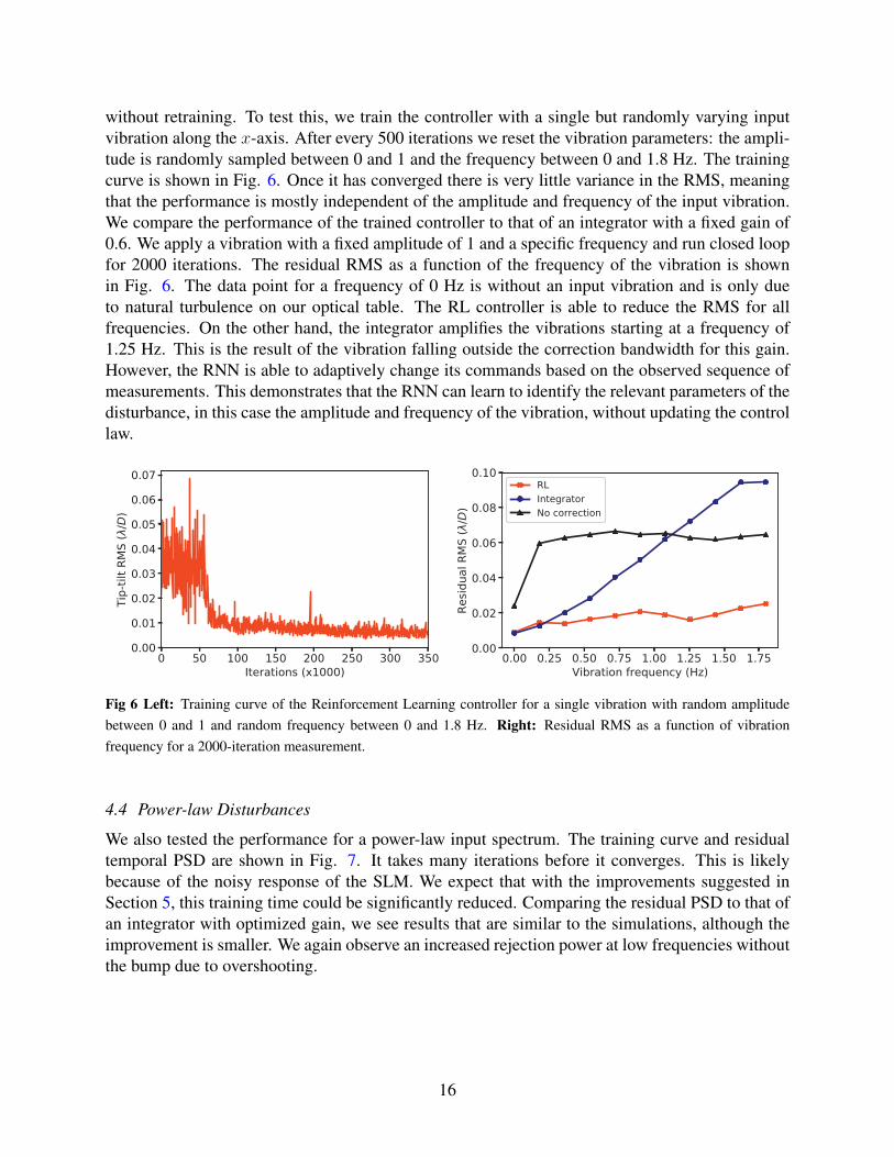
without retraining. To test this, we train the controller with a single but randomly varying inputvibration along the x-axis. After every 500 iterations we reset the vibration parameters: the ampli-tude is randomly sampled between 0 and 1 and the frequency between 0 and 1.8 Hz. The trainingcurve is shown in Fig. 6. Once it has converged there is very little variance in the RMS, meaningthat the performance is mostly independent of the amplitude and frequency of the input vibration.We compare the performance of the trained controller to that of an integrator with a fixed gain of0.6. We apply a vibration with a fixed amplitude of 1 and a specific frequency and run closed loopfor 2000 iterations. The residual RMS as a function of the frequency of the vibration is shownin Fig. 6. The data point for a frequency of 0 Hz is without an input vibration and is only dueto natural turbulence on our optical table. The RL controller is able to reduce the RMS for allfrequencies. On the other hand, the integrator amplifies the vibrations starting at a frequency of1.25 Hz. This is the result of the vibration falling outside the correction bandwidth for this gain.However, the RNN is able to adaptively change its commands based on the observed sequence ofmeasurements. This demonstrates that the RNN can learn to identify the relevant parameters of thedisturbance, in this case the amplitude and frequency of the vibration, without updating the controllaw.

Fig 6 Left: Training curve of the Reinforcement Learning controller for a single vibration with random amplitudebetween 0 and 1 and random frequency between 0 and 1.8 Hz. Right: Residual RMS as a function of vibrationfrequency for a 2000-iteration measurement.

4.4 Power-law Disturbances

We also tested the performance for a power-law input spectrum. The training curve and residualtemporal PSD are shown in Fig. 7. It takes many iterations before it converges. This is likelybecause of the noisy response of the SLM. We expect that with the improvements suggested inSection 5, this training time could be significantly reduced. Comparing the residual PSD to that ofan integrator with optimized gain, we see results that are similar to the simulations, although theimprovement is smaller. We again observe an increased rejection power at low frequencies withoutthe bump due to overshooting.

16

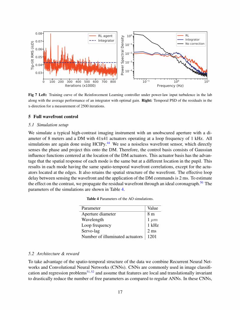
Fig 7 Left: Training curve of the Reinforcement Learning controller under power-law input turbulence in the labalong with the average performance of an integrator with optimal gain. Right: Temporal PSD of the residuals in thex-direction for a measurement of 2500 iterations.

5 Full wavefront control

5.1 Simulation setup

We simulate a typical high-contrast imaging instrument with an unobscured aperture with a di-ameter of 8 meters and a DM with 41x41 actuators operating at a loop frequency of 1 kHz. Allsimulations are again done using HCIPy.44 We use a noiseless wavefront sensor, which directlysenses the phase and project this onto the DM. Therefore, the control basis consists of Gaussianinfluence functions centered at the location of the DM actuators. This actuator basis has the advan-tage that the spatial response of each mode is the same but at a different location in the pupil. Thisresults in each mode having the same spatio-temporal wavefront correlations, except for the actu-ators located at the edges. It also retains the spatial structure of the wavefront. The effective loopdelay between sensing the wavefront and the application of the DM commands is 2 ms. To estimatethe effect on the contrast, we propagate the residual wavefront through an ideal coronagraph.50 Theparameters of the simulations are shown in Table 4.

Table 4 Parameters of the AO simulations.

Parameter ValueAperture diameter 8 mWavelength 1 µmLoop frequency 1 kHzServo-lag 2 msNumber of illuminated actuators 1201

5.2 Architecture & reward

To take advantage of the spatio-temporal structure of the data we combine Recurrent Neural Net-works and Convolutional Neural Networks (CNNs). CNNs are commonly used in image classifi-cation and regression problems51, 52 and assume that features are local and translationally invariantto drastically reduce the number of free parameters as compared to regular ANNs. In these CNNs,

17

kernels are convolved with the input data to obtain the activation in the next layer. In our case thismeans that we assume that each actuator has the same spatial response, and only close-by actu-ators are important for the prediction in the next step. We use a Convolutional Long Short-TermMemory (ConvLSTM) layer.53 This is equivalent to a LSTM for each actuator with a local fieldof view and shared weights between the actuators. The recurrent part of the Convolutional LSTMis illustrated in Figure 8. In the case of a 1x1 kernel size, we would have the same decoupledcontrol law for each individual actuator. However, this would not allow the algorithm to captureany spatial correlations in the data. Although these spatial correlations are found to be small inon-sky telemetry data for wind velocities <10 m/s on short timescales,20 they may become moreimportant for higher wind speeds or longer timescales. Furthermore, they may help in identifyingthe direction of the wind flow or to mitigate noise.

Fig 8 Illustration of the recurrent part of a Convolutional LSTM layer. The output at time t is determined by a localfield of view of the memory states mt−1 and the local inputs.

As the reward, we would ideally want to directly optimize the Strehl ratio or the post-coronagraphiccontrast in the science image. However, the accurate estimation of these quantities at kHz frequen-cies could be difficult. Therefore we use the squared residual wavefront error as the reward. Thisresidual wavefront error is calculated from the WFS measurements. A disadvantage of this is thatthe reward suffers from the same limitations as the WFS. For example, it means that the algorithmis insensitive to modes to which the WFS is blind and suffers from the same aliasing effects asthe WFS. Instead of using a single scalar as reward, we use a 2D reward map, with the squaredresidual error of each actuator mode at the actuator’s location. This allows us to use a fully con-volutional model for the critic, where only close-by actuators are considered when estimating theloss. This results in less free parameters and the access to more and localized information, leadingto decreased training times as opposed to a global metric.

The input to our controller is the residual wavefront errors ot and previous incremental DMcommands at at the location of the actuator, concatenated along the depth, the number of inputsfor each actuator. This means the input is an array of shape 41x41x2 for each time step. Forunused actuators outside the pupil, we fill the array with zeros. Our actor architecture consists ofa Convolutional LSTM layer with 16 3x3 kernels. After that, we have two regular convolutionallayers with 8 and 1 3x3 kernels, respectively, which provide the new incremental DM commandsat. For the critic, we again have a Convolutional LSTM layer with 16 3x3 kernels. After that weconcatenate the DM commands to the output of the Convolutional LSTM. This is followed by threeregular convolutional layers with 16, 8 and 1 3x3 kernels, respectively. The output of the critic isa 41x41x1 map of the expected return for each actuator. All convolutional layers use the tanhactivation function except for the last layer of the Critic, which uses a linear activation function.

18

Table 5 Neural Network architectures of the actor and critic used for the full wavefront control.

Layer type Kernel size Kernels Input shape Activation functionA

ctor ConvLSTM 3x3 16 (41, 41, 2) Tanh

Conv 3x3 8 (41, 41, 16) TanhConv 3x3 1 (41, 41, 8) Tanh

Layer type Kernel size Kernels Input shape Activation function

Cri

tic

ConvLSTM 3x3 16 (41, 41, 2) TanhConcatenate - - (41, 41,16), (41,41, 1) -

Conv 3x3 16 (41, 41, 17) TanhConv 3x3 8 (41, 41, 16) TanhConv 3x3 1 (41, 41, 8) Linear

The architectures are summarized in Table 5. Both models have ∼12,000 free parameters. Again,we have not done an optimization of the architecture or hyperparameters.

5.2.1 Algorithm improvements

Instead of starting with a randomly initialized control law, as in our tip-tilt control, we pre-trainthe actor using supervised learning to mimic an integral controller with a sub-optimal gain of 0.4.This slightly reduces the training time. In addition, we add regularization to the DM commands topenalize the controller for potentially adding unsensed modes. We do this by adding an L2 penaltyterm on the norm of the incremental DM commands to the loss function:

J(θ) = E[R]− 1

2λE[a2], (16)

where λ is the strength of the regularization. The new policy gradient then becomes:

∇θJ(θ) = E[(∇aQω(s, a)− λa)∇θπθ(s)]. (17)

Finally, we slightly alter the training procedure. Before doing the truncated backpropagationthrough time, we first propagate the 10 previous states through the models. This ensures that thememory states are initialized correctly. Initialization was less of an issue for the tip-tilt control asthe TBTT length was longer and therefore the initial timesteps contributed less to the total gradientas opposed to full AO control.

The hyperparameters for the algorithm used throughout this section are listed in Table 6. Anotable change compared to the tip-tilt control is the lower discount factor γ because the optimiza-tion horizon does not need to be long. This is because of the monotonic nature of the reward inthe absolute wavefront error; a command that decreases the wavefront error in the short term isalso the best in the long-term. We still have to use γ > 0 because of the delay in the commandsand reward. We also use a much higher target soft update τ and noise decay ζ , which both lead todecreased training times without giving up too much stability.

19

Table 6 Hyperparameters used for the full wavefront controlParameter Value

Actor learning rate 10−5

Critic learning rate 10−3

Target network soft update τ 0.1Discount factor γ 0.9

Batch size 32TBTT length l 20 ms

Action regularization λ 10−3

Initial exploration σ0 0.5 radExploration decay ζ 0.1

Episode length 1000 iterationsNumber of training steps per episode 1000

5.3 Stationary turbulence

First, we test the algorithm for input turbulence with stationary parameters. We simulate an atmo-sphere consisting of two layers of frozen-flow turbulence: A ground layer with a horizontal windspeed of 10 m/s with an r0 of 15 cm at 500 nm and a jet stream layer with a wind speed of 30 m/sat an angle of 45 degrees with an r0 of 20 cm at 500 nm. Here, an angle of 0 degrees correspondsto the turbulence flowing from left to right across the pupil. The average raw contrast behind theideal coronagraph within the control radius during the training is shown in Figure 9. After trainingwe test the algorithm without exploration noise. Figure 10 shows the resulting coronagraphic focalplane image for a 10-second simulation for our RL controller and an integrator with optimizedgain. The gain of the integrator was optimized by running in closed loop for 3 seconds to deter-mine the gain corresponding to the largest Strehl ratio. We find an optimal gain of 0.55 for theintegrator. Figure 9 shows the radially averaged raw contrast profile for these images. The rawcontrast is calculated as the average intensity in that radial bin divided by the Strehl ratio of thenon-coronagraphic focal plane image. We observe an increase in raw contrast of up to two ordersof magnitudes at small separations as compared to the integrator. Also shown is the contrast curvefor an ideal controller, which perfectly removes all wavefront errors that can be fitted with the DMat each timestep, without any delay.

5.4 Non-stationary turbulence

One may wonder if the algorithm can learn to adapt to changing turbulence conditions on its own.To explore this, we train the algorithm under a variety of conditions. We randomly reset the windspeed and direction every second. The wind speed is uniformly sampled between 10 and 40 m/s,and we allow all angles for the wind direction. Only a single layer of frozen-flow turbulence isused in these simulations. The training curve is shown in Figure 11. After training, we test thealgorithm for specific wind speeds and randomly sampled directions. The resulting focal planeimages and contrast curves for a 10-second simulation are shown in Figure 12.

Our results indicate that the controller improves the contrast for all wind velocities and direc-tions in these simulations. This demonstrates that the controller is able to learn to adapt to changesin the spatio-temporal PSD as a result of a different wind speed or angle. The controller thereforedoes not necessarily need online learning, in contrast to most other predictive control algorithms.

20

0 5 10 15 20Angular separation ( /D)

10 6

10 5

10 4

10 3

Raw

Cont

rast

RLIntegratorIdeal

0 10 20 30 40 50 60Time (s)

10 5

10 4

10 3

Aver

age

raw

cont

rast

RLIntegrator

Fig 9 Left: Evolution of the average raw contrast after an ideal coronagraph within the control radius during thetraining of the RL controller for turbulence consisting of two layers of frozen-flow turbulence. Right: Raw contrastcurves for a 10-second integration of the focal plane for the simulations with a two-layer atmosphere.

20 10 0 10 20X [ /D]

20

10

0

10

20

Y [

/D]

RL

20 10 0 10 20X [ /D]

Integrator

5.0

4.5

4.0

3.5

3.0

2.5

2.0Log raw contrast

Fig 10 10-second integration of the focal plane after an ideal coronagraph for the simulations with an atmosphereconsisting of two layers of frozen-flow turbulence.

21

0 20 40 60 80 100 120 140Time (s)

10 5

10 4

10 3

10 2

Aver

age

raw

cont

rast

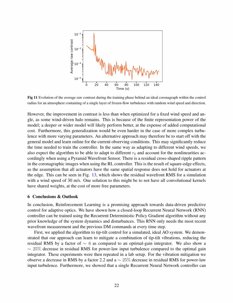
Fig 11 Evolution of the average raw contrast during the training phase behind an ideal coronagraph within the controlradius for an atmosphere containing of a single layer of frozen-flow turbulence with random wind speed and direction.

However, the improvement in contrast is less than when optimized for a fixed wind speed and an-gle, as some wind-driven halo remains. This is because of the finite representation power of themodel; a deeper or wider model will likely perform better, at the expense of added computationalcost. Furthermore, this generalization would be even harder in the case of more complex turbu-lence with more varying parameters. An alternative approach may therefore be to start off with thegeneral model and learn online for the current observing conditions. This may significantly reducethe time needed to train the controller. In the same way as adapting to different wind speeds, wealso expect the algorithm to be able to adapt to different r0 and account for the nonlinearities ac-cordingly when using a Pyramid Wavefront Sensor. There is a residual cross-shaped ripple patternin the coronagraphic images when using the RL controller. This is the result of square-edge effects,as the assumption that all actuators have the same spatial response does not hold for actuators atthe edge. This can be seen in Fig. 13, which shows the residual wavefront RMS for a simulationwith a wind speed of 30 m/s. One solution to this might be to not have all convolutional kernelshave shared weights, at the cost of more free parameters.

6 Conclusions & Outlook

In conclusion, Reinforcement Learning is a promising approach towards data-driven predictivecontrol for adaptive optics. We have shown how a closed-loop Recurrent Neural Network (RNN)controller can be trained using the Recurrent Deterministic Policy Gradient algorithm without anyprior knowledge of the system dynamics and disturbances. This RNN only needs the most recentwavefront measurement and the previous DM commands at every time step.

First, we applied the algorithm to tip-tilt control for a simulated, ideal AO system. We demon-strated that our approach can learn to mitigate a combination of tip-tilt vibrations, reducing theresidual RMS by a factor of ∼ 6 as compared to an optimal-gain integrator. We also show a∼ 25% decrease in residual RMS for power-law input turbulence compared to the optimal gainintegrator. These experiments were then repeated in a lab setup. For the vibration mitigation weobserve a decrease in RMS by a factor 2.2 and a ∼ 25% decrease in residual RMS for power-lawinput turbulence. Furthermore, we showed that a single Recurrent Neural Network controller can

22

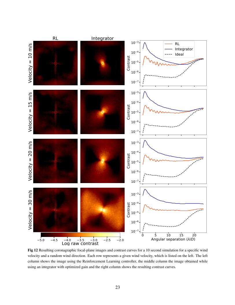
Fig 12 Resulting coronagraphic focal-plane images and contrast curves for a 10 second simulation for a specific windvelocity and a random wind direction. Each row represents a given wind velocity, which is listed on the left. The leftcolumn shows the image using the Reinforcement Learning controller, the middle column the image obtained whileusing an integrator with optimized gain and the right column shows the resulting contrast curves.

23

Wind direction

Fig 13 Residual wavefront RMS for a wind speed of 30 m/s with the controller trained on random wind directions.

mitigate a vibration with varying amplitude and frequency without needing online updating of thecontrol parameters.

Secondly, we showed in simulations how the algorithm can be applied to the control of ahigh-order DM. We showed that for an atmosphere consisting of a ground layer and a jet-streamlayer, the algorithm can improve the contrast at small separations by two orders of magnitude ascompared to an optimal-gain integrator. Furthermore, when the controller is trained over a varietyof observing conditions, it is able to adapt to changes in the wind speed and direction withoutneeding online updating of the control law. This relaxes the real-time computational demand thatwould be required to update the control law given the constantly changing atmospheric conditions.It also simplifies the implementation because control and learning can be decoupled. However, theobtained contrast is lower than when trained for stationary conditions. A deeper or wider modelmay improve its ability to generalize and perform under varying conditions, at the expense of addedcomputational time.

We have not considered the effect of photon noise on the performance of the algorithm. Asthe noise affects both the state and the reward, we expect that this will increase the amount of dataneeded to train the controller. Future research should test the effect of noise on the performanceof the controller. The algorithm should also be tested with a nonlinear wavefront sensor, such asthe pyramid wavefront sensor, because our approach has the advantage of easily accommodating anonlinear control law. Furthermore, the algorithm is off-policy, meaning that we can train on datathat is not collected with the current optimal control law. We can therefore use historical telemetrydata collected using an integrator to train the controller. It should be investigated if this can alreadyprovide a good controller or if we need to learn online.

Although we have shown the potential of Reinforcement Learning for closed-loop predictivecontrol, there are a few more practical considerations. First is the complexity of the implementa-tion of the algorithm on real-time controllers (RTC) at actual telecopes, because current RTCs areoften not compatible with the Deep Learning interfaces used in this paper. Another considerationis the computational cost. Although prediction is easily within the capabilities of current RTCsbecause of the partially decoupled approach, online learning with backpropagation will be compu-tationally very challenging. For example, the full training process, including optical simulationsand gradient updates, for the full wavefront control in the stationary case (see Section 5.3) took

24

about 4 hours using the NVIDIA Tesla K80 GPU offered by Google Colab. While this can be spedup significantly by the use of multiple GPU’s or specialized hardware, training times are likelyto increase under more complex turbulence and with real noise. However, we have shown thatthe algorithm can learn to perform under varying conditions, allowing control and training to bedecoupled, making the computational cost of training less of an issue. Alternatively, one could usethe generalized model and finetune it for the current observing conditions, significantly reducingthe training time. Another consideration is the stability of the learning algorithm and controller.Since we are using a sophisticated nonlinear controller, it is difficult to give performance guaran-tees. Furthermore, changing the hyperparameters can significantly influence the learning stabilityof the algorithm.

Acknowledgements

We wish to thank the reviewers for their feedback, which has resulted in improvements of thiswork. R.L. acknowledges funding from the European Research Council (ERC) under the Euro-pean Union’s Horizon 2020 research and innovation program under grant agreement No 694513.Support for this work was provided by NASA through the NASA Hubble Fellowship grant #HST-HF2-51436.001-A awarded by the Space Telescope Science Institute, which is operated by theAssociation of Universities for Research in Astronomy, Incorporated, under NASA contract NAS5-26555. Part of this work was already presented in Ref. 54.

Disclosures

The authors declare no conflict of interest.

References1 O. Guyon, “Extreme adaptive optics,” Annual Review of Astronomy and Astrophysics 56(1),

315–355 (2018).2 F. Cantalloube, O. J. Farley, J. Milli, et al., “Wind-driven halo in high-contrast images: I.

Analysis of the focal-plane images of SPHERE,” Astronomy and Astrophysics 638 (2020).3 J. Lozi, O. Guyon, N. Jovanovic, et al., “Characterizing vibrations at the Subaru Telescope

for the Subaru coronagraphic extreme adaptive optics instrument,” Journal of AstronomicalTelescopes, Instruments, and Systems 4(4), 1–13 (2018).

4 M. Hartung, T. Hayward, L. Saddlemyer, et al., “On-sky vibration environment for the Gem-ini Planet Imager and mitigation effort,” in Adaptive Optics Systems IV, E. Marchetti, L. M.Close, and J.-P. Veran, Eds., 9148, 202 – 213, International Society for Optics and Photonics,SPIE (2014).

5 J.-F. Sauvage, T. Fusco, C. Petit, et al., “SAXO, the eXtreme Adaptive Optics System ofSPHERE: overview and calibration procedure,” in Adaptive Optics Systems II, B. L. Eller-broek, M. Hart, N. Hubin, et al., Eds., 7736, 175 – 184, International Society for Optics andPhotonics, SPIE (2010).

6 J. P. Lloyd and A. Sivaramakrishnan, “Tip-Tilt Error in Lyot Coronagraphs,” The Astrophys-ical Journal 621, 1153–1158 (2005).

25

7 D. Mawet, L. Pueyo, D. Moody, et al., “The Vector Vortex Coronagraph: sensitivity to cen-tral obscuration, low-order aberrations, chromaticism, and polarization,” in Modern Tech-nologies in Space- and Ground-based Telescopes and Instrumentation, E. Atad-Ettedgui andD. Lemke, Eds., 7739, 378–390, International Society for Optics and Photonics, SPIE (2010).

8 E. Gendron and P. Lena, “Astronomical adaptive optics. I. Modal control optimization,” As-tronomy and Astrophysics 291(1), 337–337 (1994).

9 E. Gendron and P. Lena, “Astronomical adaptive optics. II. Experimental results of an opti-mized modal control.,” Astronomy and Astrophysics Supplement Series 111(111), 153 (1995).

10 R. N. Paschall and D. J. Anderson, “Linear quadratic Gaussian control of a deformable mir-ror adaptive optics system with time-delayed measurements,” Applied Optics 32(31), 6347(1993).

11 C. Correia, J.-P. Veran, and G. Herriot, “Advanced vibration suppression algorithms in adap-tive optics systems,” Journal of the Optical Society of America A 29(3), 185 (2012).

12 C. Petit, J.-M. Conan, C. Kulcsar, et al., “First laboratory validation of vibration filtering withLQG control law for Adaptive Optics,” Optics Express 16(1), 87 (2008).

13 G. Sivo, C. Kulcsar, J.-M. Conan, et al., “First on-sky SCAO validation of full LQG controlwith vibration mitigation on the CANARY pathfinder,” Optics Express 22(19), 23565 (2014).

14 C. Petit, J.-F. Sauvage, T. Fusco, et al., “SPHERE eXtreme AO control scheme: final per-formance assessment and on sky validation of the first auto-tuned LQG based operationalsystem,” in Adaptive Optics Systems IV, E. Marchetti, L. M. Close, and J.-P. Veran, Eds.,9148, 214 – 230, International Society for Optics and Photonics, SPIE (2014).

15 C. Correia, H.-F. Raynaud, C. Kulcsar, et al., “On the optimal reconstruction and control ofadaptive optical systems with mirror dynamics,” Journal of the Optical Society of America A27(2), 333 (2010).

16 L. A. Poyneer, D. W. Palmer, B. Macintosh, et al., “Performance of the Gemini Planet Im-ager’s adaptive optics system,” Applied Optics 55(2), 323 (2016).

17 C. Dessenne, P.-Y. Madec, and G. Rousset, “Modal prediction for closed-loop adaptive op-tics,” Optics Letters 22(20), 1535 (1997).

18 O. Guyon and J. Males, “Adaptive Optics Predictive Control with Empirical OrthogonalFunctions (EOFs),” (2017).

19 R. Jensen-Clem, C. Z. Bond, S. Cetre, et al., “Demonstrating predictive wavefront controlwith the Keck II near-infrared pyramid wavefront sensor,” in Techniques and Instrumentationfor Detection of Exoplanets IX, S. B. Shaklan, Ed., 11117, 275 – 284, International Societyfor Optics and Photonics, SPIE (2019).

20 M. A. Van Kooten, N. Doelman, and M. Kenworthy, “Robustness of prediction for extremeadaptive optics systems under various observing conditions: An analysis using VLT/SPHEREadaptive optics data,” Astronomy and Astrophysics 636, 81 (2020).

21 V. Deo, E. Gendron, G. Rousset, et al., “A telescope-ready approach for modal compensationof pyramid wavefront sensor optical gain,” Astronomy & Astrophysics 629, A107 (2019).

22 A. P. Wong, B. R. M. Norris, P. G. Tuthill, et al., “Predictive control for adaptive optics usingneural networks,” Journal of Astronomical Telescopes, Instruments, and Systems 7(1), 1–22(2021).

26

23 R. Swanson, M. Lamb, C. M. Correia, et al., “Closed Loop Predictive Control of AdaptiveOptics Systems with Convolutional Neural Networks,” Monthly Notices of the Royal Astro-nomical Society (2021).

24 S. Y. Haffert, J. R. Males, L. M. Close, et al., “Data-driven subspace predictive control ofadaptive optics for high-contrast imaging,” Journal of Astronomical Telescopes, Instruments,and Systems 7(2), 1 – 22 (2021).

25 M. van Kooten, N. Doelman, and M. Kenworthy, “Impact of time-variant turbulence behavioron prediction for adaptive optics systems,” J. Opt. Soc. Am. A 36, 731–740 (2019).

26 M. Gray, C. Petit, S. Rodionov, et al., “Local ensemble transform Kalman filter, a fast non-stationary control law for adaptive optics on ELTs: theoretical aspects and first simulationresults,” Optics Express 22(17), 20894 (2014).

27 X. Liu, T. Morris, C. Saunter, et al., “Wavefront prediction using artificial neural networksfor open-loop adaptive optics,” Monthly Notices of the Royal Astronomical Society 496(1),456–464 (2020).

28 R. Landman and S. Y. Haffert, “Nonlinear wavefront reconstruction with convolutional neuralnetworks for Fourier-based wavefront sensors,” Optics Express 28(11), 16644 (2020).

29 B. R. M. Norris, J. Wei, C. H. Betters, et al., “An all-photonic focal-plane wavefront sensor,”Nature Communications (2020), 1–9 (2020).

30 R. Swanson, M. Lamb, C. Correia, et al., “Wavefront reconstruction and prediction withconvolutional neural networks,” in Adaptive Optics Systems VI, L. M. Close, L. Schreiber,and D. Schmidt, Eds., 10703, 481 – 490, International Society for Optics and Photonics,SPIE (2018).

31 V. M. Radhakrishnan, C. U. Keller, and N. Doelman, “Optimization of contrast in adaptiveoptics for exoplanet imaging,” in Adaptive Optics Systems VI, L. M. Close, L. Schreiber, andD. Schmidt, Eds., 10703, 1211 – 1217, International Society for Optics and Photonics, SPIE(2018).

32 H. Sun, N. J. Kasdin, and R. Vanderbei, “Identification and adaptive control of a high-contrastfocal plane wavefront correction system,” Journal of Astronomical Telescopes, Instruments,and Systems 4(04), 1 (2018).

33 J. Nousiainen, C. Rajani, M. Kasper, et al., “Adaptive optics control using model-based rein-forcement learning,” Optics Express 29, 15327 (2021).

34 R. S. Sutton and A. G. Barto, Reinforcement Learning: An Introduction, MIT Press (2018).35 K. Arulkumaran, M. P. Deisenroth, M. Brundage, et al., “Deep reinforcement learning: A

brief survey,” IEEE Signal Processing Magazine 34(6), 26–38 (2017).36 D. Silver, G. Lever, N. Heess, et al., “Deterministic policy gradient algorithms,” 31st Inter-

national Conference on Machine Learning, ICML 2014 1, 605–619 (2014).37 T. P. Lillicrap, J. J. Hunt, A. Pritzel, et al., “Continuous control with deep reinforcement

learning,” 4th International Conference on Learning Representations, ICLR 2016 (2016).38 I. J. Goodfellow, Y. Bengio, and A. Courville, Deep Learning, MIT Press, Cambridge, MA,

USA (2016). http://www.deeplearningbook.org.39 R. Bellman, “The theory of dynamic programming,” Bulletin of the American Mathematical

Society 60(6), 503 – 515 (1954).

27

40 D. Wierstra, A. Foerster, J. Peters, et al., “Solving deep memory pomdps with recurrentpolicy gradients,” in Proceedings of the 17th International Conference on Artificial NeuralNetworks, ICANN’07, 697–706, Springer-Verlag, (Berlin, Heidelberg) (2007).

41 N. Heess, J. J. Hunt, T. P. Lillicrap, et al., “Memory-based control with recurrent neuralnetworks,” (2015).

42 A. Graves, A. Mohamed, and G. Hinton, “Speech recognition with deep recurrent neural net-works,” in 2013 IEEE International Conference on Acoustics, Speech and Signal Processing,6645–6649 (2013).

43 S. Hochreiter and J. Urgen Schmidhuber, “Long Short-term Memory,” Neural Computation9(8), 17351780 (1997).

44 E. H. Por, S. Y. Haffert, V. M. Radhakrishnan, et al., “High Contrast Imaging for Python(HCIPy): an open-source adaptive optics and coronagraph simulator,” in Adaptive OpticsSystems VI, Proc. SPIE 10703, 152 (2018).

45 D. P. Kingma and J. L. Ba, “Adam: A method for stochastic optimization,” 3rd InternationalConference on Learning Representations, ICLR 2015 (2015).

46 M. Abadi, A. Agarwal, P. Barham, et al., “TensorFlow: Large-scale machine learning onheterogeneous systems,” (2015). Software available from tensorflow.org.

47 F. Chollet et al., “Keras.” https://keras.io (2015).48 P. D. Welch, “The Use of Fast Fourier Transform for the Estimation of Power Spectra,” Dig-

ital Signal Processing (2), 532–574 (1975).49 J.-M. Conan, G. Rousset, and P.-Y. Madec, “Wave-front temporal spectra in high-resolution

imaging through turbulence,” J. Opt. Soc. Am. A 12, 1559–1570 (1995).50 O. Guyon, E. A. Pluzhnik, M. J. Kuchner, et al., “Theoretical Limits on Extrasolar Terrestrial

Planet Detection with Coronagraphs,” The Astrophysical Journal Supplement Series 167(1),81–99 (2006).

51 A. Krizhevsky, I. Sutskever, and G. E. Hinton, “Imagenet classification with deep convolu-tional neural networks,” Advances in Neural Information Processing Systems 25, 1097–1105(2012).

52 K. He, X. Zhang, S. Ren, et al., “Deep residual learning for image recognition,” (2015).53 X. Shi, Z. Chen, H. Wang, et al., “Convolutional lstm network: A machine learning approach

for precipitation nowcasting,” Advances in Neural Information Processing Systems 28, 802–810 (2015).

54 R. Landman, S. Y. Haffert, V. M. Radhakrishnan, et al., “Self-optimizing adaptive optics con-trol with reinforcement learning,” in Adaptive Optics Systems VII, L. Schreiber, D. Schmidt,and E. Vernet, Eds., 11448, 842 – 856, International Society for Optics and Photonics, SPIE(2020).

Rico Landman is a PhD candidate at Leiden Observatory working on direct imaging and spec-troscopy of exoplanets. He received his BS degrees in physics and astronomy and MS degree inastronomy from Leiden University in 2018 and 2020, respectively.

Sebastiaan Y. Haffert is a NASA Hubble Postdoctoral Fellow at the University of Arizona’s Stew-ard Observatory. His research focuses on high-spatial and high-spectral resolution instrumentationfor exoplanet characterization.

28

Vikram M. Radhakrishnan is a PhD candidate at Leiden Observatory working on innovativecontrol approaches to high-contrast imaging.

Christoph U. Keller is a Professor of Experimental Astrophysics at Leiden Observatory. He spe-cializes in developing innovative optical instruments for astronomy, remote sensing and biomedicalimaging.

List of Figures1 Visual overview of the algorithm. The black line indicates forward propagation.

The green and red lines indicate how we backpropagate the gradients to update thecritic and the actor, respectively.

2 Top left: Training curve of the Reinforcement Learning controller under inputdisturbance consisting of three vibrations along both directions. Also shown isthe average performance of an integrator with optimal gain. Top right: TemporalPSD of the residuals in the x-direction for a simulation of 10 seconds. Note that thelines of the input spectrum and integrator overlap at the peak at 37 Hz. Bottom:Residuals for the different controllers in the x-direction for a 500 ms simulation.

3 Left: Training curve of the Reinforcement Learning controller under power-lawinput turbulence and the average performance of an integrator with optimal gain.Right: Temporal PSD of the residuals in the x-direction for a simulation of 10seconds.

4 Lab setup to test the RL control algorithm with lenses L0-L4, Polarizers P1 andP2, a Spatial Light Modulator (SLM) and a camera (CAM). Insets: (a) Measuredtilt in the focal plane as a function of the applied phase gradient on the SLM. (b)Measured Point Spread Function for the setup.

5 Top left: Training curve of the Reinforcement Learning controller for an inputspectrum consisting of 3 vibrations along each direction in the lab. For compar-ison, we show the average performance of an integrator with optimal gain. Topright: Temporal PSD of the residuals in the x-direction for a measurement of 2500iterations. Bottom: Residuals for the two controllers in the x-direction for a 500-iteration measurement.

6 Left: Training curve of the Reinforcement Learning controller for a single vibra-tion with random amplitude between 0 and 1 and random frequency between 0 and1.8 Hz. Right: Residual RMS as a function of vibration frequency for a 2000-iteration measurement.

7 Left: Training curve of the Reinforcement Learning controller under power-lawinput turbulence in the lab along with the average performance of an integratorwith optimal gain. Right: Temporal PSD of the residuals in the x-direction for ameasurement of 2500 iterations.

8 Illustration of the recurrent part of a Convolutional LSTM layer. The output at timet is determined by a local field of view of the memory states mt−1 and the localinputs.

29

9 Left: Evolution of the average raw contrast after an ideal coronagraph within thecontrol radius during the training of the RL controller for turbulence consisting oftwo layers of frozen-flow turbulence. Right: Raw contrast curves for a 10-secondintegration of the focal plane for the simulations with a two-layer atmosphere.

10 10-second integration of the focal plane after an ideal coronagraph for the simula-tions with an atmosphere consisting of two layers of frozen-flow turbulence.

11 Evolution of the average raw contrast during the training phase behind an idealcoronagraph within the control radius for an atmosphere containing of a singlelayer of frozen-flow turbulence with random wind speed and direction.

12 Resulting coronagraphic focal-plane images and contrast curves for a 10 secondsimulation for a specific wind velocity and a random wind direction. Each rowrepresents a given wind velocity, which is listed on the left. The left column showsthe image using the Reinforcement Learning controller, the middle column theimage obtained while using an integrator with optimized gain and the right columnshows the resulting contrast curves.

13 Residual wavefront RMS for a wind speed of 30 m/s with the controller trained onrandom wind directions.

List of Tables1 Overview and explanation of the various terms used in the Reinforcement Learning

(RL) framework.2 Neural Network architectures of the actor and critic for the tip-tilt control.3 Hyperparameters4 Parameters of the AO simulations.5 Neural Network architectures of the actor and critic used for the full wavefront

control.6 Hyperparameters used for the full wavefront control

30