SEDIMENT YIELD ESTIMATION USING MODIFIED MMF MODEL IN A GEOSPATIAL ENVIRONMENT

Proceedings of HYDRO 2013 INTERNATIONAL,

4-6 Dec 2013, IIT Madras, INDIA

1

SEDIMENT YIELD ESTIMATION USING MODIFIED MMF MODEL IN A

GEOSPATIAL ENVIRONMENT

L. Rajtantra 1, G. Vaibhav

2, N. Bhaskar

3

Abstract: Soil erosion and sediment yield estimation for a sub-watershed using

geographical information system coupled soil erosion models, such as Universal

Soil Loss Equation (USLE) or Agricultural Non-point Source Pollution model

(AGNPS) has become recent trend but erosion assessment using Modified

Morgan-Morgan-Finney (MMF) model (2008) has not been operationally applied

for Indian region.

Main objective of the study is to fetch the MMF model completely in a geospatial

framework and estimate the actual sediment yield at the sub-watershed outlet. In

the present study, this model is used for evaluating soil erosion and sediment yield

of a sub-watershed of Satluj river basin. With the help of rainfall intensity, model

calculates the kinetic energy using exponential equation for Indian condition. The

model incorporates particle size selectivity in the process of erosion, transport and

deposition. These processes are simulated separately for clay, silt and sand.

Modified MMF model also takes sediment routing into account, which increases

sediment yield estimation accuracy and allows determination of sub-watershed

contributions to the total sediment yield for entire basin. The present research work

fetches MMF model in a geospatial environment and develops a system, which can

be used to estimate the actual sediment yield of a sub-watershed with reasonable

accuracy. The suggested model has been developed for two years i.e. 1998 & 2002

and validation has been carried out for another two years such as 1995 & 1999.

The model produces satisfactory estimates of sediment yield from sub-watershed

with maximum ±36.5% and minimum ±3.93% deviation from observations.

Keywords: Modified MMF; Sediment routing; Sediment yield; GIS; Remote

sensing

REFERENCES

Kinnell, P.I.A., 1981. Rainfall intensity-kinetic energy relationships for soil loss

prediction. Soil Science Society of America Journal 45, 153–155.

Morgan, R.P.C., Duzant, J.H., 2008. Modified MMF (Morgan–Morgan–Finney) model

for evaluating effects of crops and vegetation cover on soil erosion. Earth Surface

Processes and Landforms 33, 90–106.

1

M.Tech Student, Indian Institute of Remote Sensing, Dehradun-248001, Uttrakhand, India

E-mail: [email protected] 2 Scientist „SD‟, Indian Institute of Remote Sensing, Dehradun-248001, Uttrakhand, India


E-mail: [email protected]



2

SEDIMENT YIELD ESTIMATION USING MODIFIED MMF MODEL IN A

GEOSPATIAL ENVIRONMENT

L. Rajtantra 1, G. Vaibhav

2, N. Bhaskar

3

Abstract: Soil erosion and sediment yield estimation for a sub-watershed using

geographical information system coupled soil erosion models, such as Universal

Soil Loss Equation (USLE) or Agricultural Non-point Source Pollution model

(AGNPS) has become recent trend but erosion assessment using Modified

Morgan-Morgan-Finney (MMF) model (2008) has not been operationally applied

for Indian region. In the present study, this model is used for evaluating soil

erosion and sediment yield of a sub-watershed of Satluj river basin. With the help

of rainfall intensity, model calculates the kinetic energy using exponential equation

for Indian condition. The model incorporates particle size selectivity in the process

of erosion, transport and deposition. These processes are simulated separately for

clay, silt and sand. Modified MMF model also takes sediment routing into account,

which increases sediment yield estimation accuracy and allows determination of

sub-watershed contributions to the total sediment yield for entire basin. The

present research work fetches MMF model in a geospatial environment and

develops a system, which can be used to estimate the actual sediment yield of a

sub-watershed with reasonable accuracy. The suggested model has been developed

for two years i.e. 1998 & 2002 and validation has been carried out for another two

years such as 1995 & 1999. The model produces satisfactory estimates of sediment

yield from sub-watershed with maximum ±36.5% and minimum ±3.93% deviation

from observations.

Keywords: Modified MMF; Sediment routing; Sediment yield; GIS; Remote

sensing

INTRODUCTION

Balanced ecosystems including soil, water and plant environments are essential for the

survival and welfare of mankind. However, in the past due to over exploitation in many parts

of the world, including some parts of India the ecosystems have been distressed. The

resulting imbalance in the ecosystem is revealed through various undesirable effects, such as

soil surface degradation, frequent occurrence of intense floods etc. For example, the large

scale deforestation which occurred in the Shiwalik ranges of the Indian Himalayas during

1960s caused the soil on the land surfaces to be directly exposed to the rains (Kothyari,

1996).

1

M.Tech Student, Indian Institute of Remote Sensing, Dehradun-248001, Uttrakhand, India



E-mail: [email protected]



3

This unprotected soil was readily removed from the land surface in the fragile Shiwaliks by

the combined action of rain and resulting flow (Kothyari, 1996). Soil erosion is one of the

most significant and common forms of soil degradation which has environmental and

economic impacts. Soil erosion is a complex process that is associated with rainfall,

topography, soil properties, land cover, and human activities. In order to estimate soil

erosion, sediment yield and optimize soil conservation management, many soil erosion

models have been developed. Lal (2001) and Merritt et al., 2003 summarized major soil

erosion models in their work. Erosion models such as Universal Soil Loss Equation (USLE)

and its derivatives, Revised USLE (RUSLE) and Modified USLE (MUSLE), are the most

widely used empirical models because of their minimal data and computation requirements

(Lal, 2001; Merritt et al., 2003; Lim et al., 2005; Xu et al., 2008). Generally USLE, RUSLE,

MUSLE are used for erosion studies (Jones et al., 1996; Di Stefano et al., 2000; Ustun, 2008;

Gitas et al., 2009; Jain and Das, 2009). Even Morgan-Morgan-Finney (MMF) model and

modified MMF have been used (Morgan, 1982; Morgan et al., 1998; Morgan, 2001) but there

is a number of limitations in the previous models such as USLE applies only to sheet erosion

since the source of energy is rain; so it never applies to linear or mass erosion, the relations

between kinetic energy and rainfall intensity generally used in this model apply only to the

American Great Plains, and not to mountainous regions (Kinnell and Risse, 1998). Estimation

of soil erosion using RUSLE mainly affect by the individual locations because there is a

change in the specific factors which have been used in RUSLE (Renard et al., 1991). MUSLE

model has been developed for estimating the sediment load produced by each storm, which

takes into account not rainfall erosivity but the volume of runoff but it also has some

limitation such as it is not incorporating detachment by runoff and raindrop impact (Arekhi et

al., 2012). However, for Satluj basin estimation of sedimentation rate in Bhakra reservoir has

been carried out using remote sensing (Jain et al., 2002). It is only for the reservoir and no

catchment study has been done.

As compared to other soil erosion models, Modified MMF (Morgan and Duzant, 2008

version) model has some distinguishing features such as it incorporates effects of vegetation

cover on erosion prediction, model performs particle size selectivity in the processes of

detachment, transport, and deposition and these processes are simulated separately for clay,

silt and sand, In Modified MMF deposition is modeled through a particle fall number

(Tollner, 1973) which takes into account of particle settling velocity, flow velocity, flow

depth and slope length. There is no need to use a voluminous data in this respective model

and it is very simple to couple with GIS, moreover it is always an ease to work with

geospatial domain as the main perspective of the research. The aspect of routing of runoff and

sediment has been performed via programming (PYTHON 2.6.5) which is further been used

in the GIS environment.

The paper documents the estimation of actual sediment yield for a sub-watershed of Satluj

basin with the help of GIS coupled Modified MMF (Morgan and Duzant, 2008) model.

STUDY AREA

The geographical limits of Satluj basin lies between Latitudes 30o

N and 33o N and

Longitudes 76o E and 83

o E up to Bhakra dam (Fig. 1). Satluj basin is one of the major river

basin of Indus system (Gosain et al., 2011). It is a typical basin considered from geographical

and geological point of view, covering major parts of Nari Khorsam region in Tibet, certain



4

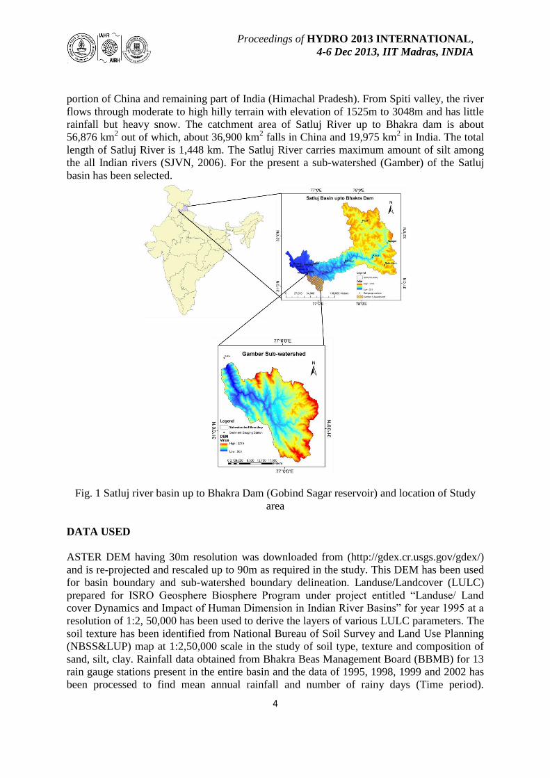
portion of China and remaining part of India (Himachal Pradesh). From Spiti valley, the river

flows through moderate to high hilly terrain with elevation of 1525m to 3048m and has little

rainfall but heavy snow. The catchment area of Satluj River up to Bhakra dam is about

56,876 km2 out of which, about 36,900 km

2 falls in China and 19,975 km

2 in India. The total

length of Satluj River is 1,448 km. The Satluj River carries maximum amount of silt among

the all Indian rivers (SJVN, 2006). For the present a sub-watershed (Gamber) of the Satluj

basin has been selected.

Fig. 1 Satluj river basin up to Bhakra Dam (Gobind Sagar reservoir) and location of Study

area

DATA USED

ASTER DEM having 30m resolution was downloaded from (http://gdex.cr.usgs.gov/gdex/)

and is re-projected and rescaled up to 90m as required in the study. This DEM has been used

for basin boundary and sub-watershed boundary delineation. Landuse/Landcover (LULC)

prepared for ISRO Geosphere Biosphere Program under project entitled “Landuse/ Land

cover Dynamics and Impact of Human Dimension in Indian River Basins” for year 1995 at a

resolution of 1:2, 50,000 has been used to derive the layers of various LULC parameters. The

soil texture has been identified from National Bureau of Soil Survey and Land Use Planning

(NBSS&LUP) map at 1:2,50,000 scale in the study of soil type, texture and composition of

sand, silt, clay. Rainfall data obtained from Bhakra Beas Management Board (BBMB) for 13

rain gauge stations present in the entire basin and the data of 1995, 1998, 1999 and 2002 has

been processed to find mean annual rainfall and number of rainy days (Time period).



5

Observed data of annual sediment yield has been obtained from BBMB too. Observation has

been taken at the sediment gauging stations in alternate years and rest of the years has been

interpolated according to preceding year.

METHODOLOGY

The model can be applied to a single slope element (Pixel) or many number of elements.

However, in the present study, selected sub-watershed is sub-divided into number of elements

(91523). These elements can be arranged in a logical sequence to reflect the direction of flow

of runoff and sediment over the landscape. All layers have been inputted into the MMF

model and processed further step by step. The main steps incorporated by the MMF model

are as follows:

Estimation of Rainfall Energy

The model starts with rainfall energy estimation. The effective rainfall (Rf, mm) is calculated

from the raster map of mean annual rainfall (R, mm) after allowing the permanent

interception (PI, proportion between zero and unity) due to the vegetation cover. Slope (S,

radian) is added on the quantity of the rain received per unit area for the profound effective

rainfall estimation. All raster layers brought into the Raster calculator tool available in Arc

GIS 10.0 and final Rf map has been derived.

Rf =R× (1-PI) × (1/cosS) 1

The effective rainfall is divided into two sub categories that are direct throughfall (DT, mm)

and leaf drainage (LD, mm). Leaf drainage is directly proportional to the amount of the

effective rainfall which is intercepted by the canopy cover (CC). Canopy cover map is

available in the form of raster layer and LD was derived by multiplying Rf and CC maps.

LD = Rf × CC 2

Direct through fall then becomes the difference between the effective rainfall and the loss of

rainfall water due to leaf drainage.

DT = Rf – LD 3

The kinetic energy (KE; J m−2

mm-1

) of direct throughfall is a function of the intensity of the

erosive rain (I, mm h−1

), maximum kinetic energy content (KEmax; J m−2

mm-1

) and an amount

of direct throughfall. The relationship between kinetic energy and rainfall intensity (I) varies

with the drop-size distribution of the rainfall. In this study, formula developed by Kinnell,

(1981) (for Indian condition) has been used.

KE (DT) = DT × [KEmax {1 – a exp (- bI)}] 4

Where, a and b are empirical constants and KEmax is the maximum kinetic energy. These three

parameters have been obtained from work done by Van Dijk et al., (2002). Guide values are

basically used for the intensity of the erosive rain (I) according to geographical location.



6

They are 10 mm h−1

for temperate climates, 25 for tropical climates and 30 for strongly

seasonal climates. A value of 25 is suitable for the present study region (Kinnell, 1981).

Based on the work of Brandt (1990), by giving the following condition in raster calculator

KE (LD) map has been derived.

For PH < 0·15, KE (LD) = 0 5

For PH ≥ 0·15, KE (LD) = (15·8 × PH0·5

) − 5·87 6

The above mentioned Eq. (5) is used to prevent the kinetic energy of the leaf drainage to

becoming a negative value when Eq. (6) is extrapolated to very low plant heights. The total

kinetic energy of the effective rainfall is,

KE = KE (DT) + KE (LD) 7

Estimation of Runoff

This model is quite different from previous MMF models. It incorporates soil loss (sediment)

routing as well as runoff routing. The model divides entire watershed in a number of

elements, for this study ASTER DEM (90m, rescaled) has been taken as base map so that all

input layers created in same resolution. Element size has been taken as same as pixel size

(90×90) of base map (DEM). All the routing process has been carried out by coding

developed in PYTHON 2.6.5. The input maps for the entire process are flow direction, flow

accumulation, effective rainfall (Rf; mm), soil moisture storage capacity (Rc; mm), mean rain

per rainy day (Ro; mm), mean annual rainfall (R; mm), evaporation (E; mm), lateral

permeability of soil (LP; m/day) and slope map (s; radian). These layers have been taken as

an input for python code and give total runoff map (Q; mm) as an output.

In this model runoff starts from the pixel where flow accumulation is zero because

that pixel is not getting runoff from any other pixel. The total runoff generated on that pixel

will now become contributing runoff for another which has flow accumulation greater than

zero. The annual runoff generated on the pixel element (Qe; mm), which have no contributing

pixel can be predicted from Kirkby (1976)

Qe = Rf exp (−Rc/R0) 8

R0 is the mean rain per rain day (i.e. R/Rn, where Rn is the mean annual number of rain days),

Rf is the effective rainfall, Rc (mm) is the soil moisture storage capacity of the soil, mainly

depends upon the soil moisture content at the field capacity (MS, w/w), the bulk density of

the soil (BD, Mg m−3

), the effective hydrological depth (EHD, m), and the loss of water from

the soil through evapo-transpiration, represented by the Et/E0 ratio of the land cover.

Rc = (1000MS × BD × EHD × (Et/E0)0·5

) 9

The values of parameters have been used in Eq. 9 are based on the work of Morgan and

Duzant (2008). The runoff generated on the element having accumulation value zero will

have some interflow. This volume of interflow can be estimated from formula given by

Kirkby (1976).



7

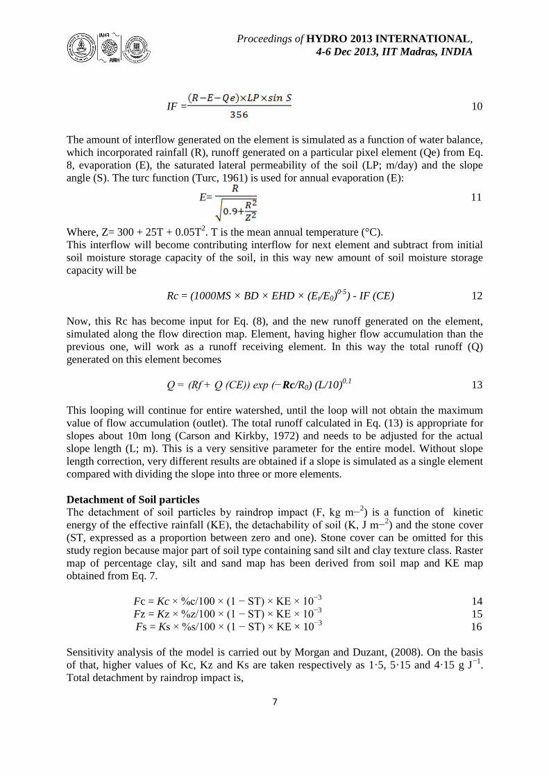
IF = 10

The amount of interflow generated on the element is simulated as a function of water balance,

which incorporated rainfall (R), runoff generated on a particular pixel element (Qe) from Eq.

8, evaporation (E), the saturated lateral permeability of the soil (LP; m/day) and the slope

angle (S). The turc function (Turc, 1961) is used for annual evaporation (E):

E= 11

Where, Z= 300 + 25T + 0.05T2. T is the mean annual temperature (°C).

This interflow will become contributing interflow for next element and subtract from initial

soil moisture storage capacity of the soil, in this way new amount of soil moisture storage

capacity will be

Rc = (1000MS × BD × EHD × (Et/E0)0·5

) - IF (CE) 12

Now, this Rc has become input for Eq. (8), and the new runoff generated on the element,

simulated along the flow direction map. Element, having higher flow accumulation than the

previous one, will work as a runoff receiving element. In this way the total runoff (Q)

generated on this element becomes

Q = (Rf + Q (CE)) exp (−Rc/R0) (L/10)0.1

13

This looping will continue for entire watershed, until the loop will not obtain the maximum

value of flow accumulation (outlet). The total runoff calculated in Eq. (13) is appropriate for

slopes about 10m long (Carson and Kirkby, 1972) and needs to be adjusted for the actual

slope length (L; m). This is a very sensitive parameter for the entire model. Without slope

length correction, very different results are obtained if a slope is simulated as a single element

compared with dividing the slope into three or more elements.

Detachment of Soil particles

The detachment of soil particles by raindrop impact (F, kg m−2) is a function of kinetic

energy of the effective rainfall (KE), the detachability of soil (K, J m−2) and the stone cover

(ST, expressed as a proportion between zero and one). Stone cover can be omitted for this

study region because major part of soil type containing sand silt and clay texture class. Raster

map of percentage clay, silt and sand map has been derived from soil map and KE map

obtained from Eq. 7.

Fc = Kc × %c/100 × (1 − ST) × KE × 10−3

14

Fz = Kz × %z/100 × (1 − ST) × KE × 10−3

15

Fs = Ks × %s/100 × (1 − ST) × KE × 10−3

16

Sensitivity analysis of the model is carried out by Morgan and Duzant, (2008). On the basis

of that, higher values of Kc, Kz and Ks are taken respectively as 1·5, 5·15 and 4·15 g J−1

.

Total detachment by raindrop impact is,



8

F = Fc + Fz + Fs 17

The detachment of soil particles (H, kg m−2

) by runoff, is a function of volume of runoff (Q),

the detachability of the soil by runoff (DR, g mm−1

), slope angle (S) and the proportion of the

soil covered by vegetation (GC) and stones (ST). Q map obtained from Eq. 13, ground cover

(GC) raster map from LULC, and slope map derived from DEM.

Hc= DRc × %c/100 × Q1·5

× (1 − (GC + ST)) × sin0·3

S × 10−3

18

Hz = DRz × %c/100 × Q1·5

× (1 − (GC + ST)) × sin0·3

S × 10−3

19

Hs = DRs × %c/100 × Q1·5

× (1 − (GC + ST)) × sin0·3

S × 10−3

20

Total detachment by runoff is,

H= Hc + Hz + Hs 21

The calibrated values for DR are 2·0, 1·6 and 1·5 for the clay (c), silt (z) and sand (s)

fractions respectively, based on data from sensitivity analysis (Morgan and Duzant, 2008).

Immediate Deposition of Detached particles

Only a part of the detached sediment will be delivered to the runoff for transport, the

remainder will be deposited close to the point of detachment. The deposition of soil particles

is modeled as a function of the probability that is, a detached particle will fall to the soil

surface instead of entrained in the runoff. This probability is related to a particle fall number

(Nf, Tollner et al., 1976), which depends upon the length of the element (l), the fall velocity

of the particles (νs), the flow velocity (ν) and the flow depth (d).

Flow velocity calculations are made for four possible conditions:

a) A standard condition related to un-channeled overland flow over a smooth bare soil (νb).

b) The actual condition, which can take account of flow channeling into rills (νa).

c) A condition taking into account of the effects of the vegetation cover (νv).

d) A condition taking account of the roughness of the soil surface, as that result from tillage

(νt).

Calculations are made only for those conditions that exist for the study region where the

model is being applied. Thus, if there is no vegetation or crop cover, vv can be omitted. In

Gamber region tillage practices do not affect the sediment yield because crop acreage is less

than hill slopes and forest therefore νt has been omitted from further calculation and first three

velocities has been incorporated.

Considering the above said conditions and taking them into detail,

1. For the standard bare soil condition, flow velocity map is estimated from the Manning

equation,

vb = 1/n d0·67

S0·5

22

Where n is Manning‟s roughness coefficient and d is the flow depth (m) and slope (S) has

been taken in m/m. Values of n = 0·015 and d = 0·005 are used.



9

2. For the actual flow velocity (va), the Eq. 22 is used. If flow accumulation is >=50 the

flow depth d = 0·005, it is showing un-channeled flow. If flow accumulation between 51

to 1000 flow depth d = 0·01 showing shallow rills and if flow accumulation greater than

1000 d will be 0·25 showing deeper rills. The equation used is,

va = 1/n d0·67

S 0·5

23

3. For the vegetated conditions, flow velocity is estimated as a function of slope map (S;

m/m) and the density of the vegetation, the latter depends upon the diameter of the plant

stems (D) and the number of stems per unit area (NV) (Jin et al., 2000),

νv = S0.5

24

Raster layer of D and NV has been derived from LULC map and the values have been taken

from work done by Morgan and Duzant (2008). Now the particle fall number (Nf) map is

determined separately for each soil particle class from,

Nf(c) = l×Vs(c) / v×d 25

Nf(z) = l ×Vs (z) / v×d 26

Nf(s) = l ×Vs(s) / v×d 27

Where length of the element (l) taken as 90m, ν is velocity for bare soil condition, vegetated

condition or actual condition and d is the depth of flow used in Eq. 23. Flow velocities have

been taken from Eq. 22, 23 and 24. Fall velocities are estimated from,

νs = 28

Where δ is the diameter of the particle, ρs is the sediment density (1240 kg m−3

), ρ is the flow

density (typically 1100 kg m−3

) for runoff on hill slopes (Abrahams et al., 2001), g is

gravitational acceleration (taken as 9·81 m s−2

) and η is the fluid viscosity (nominally 0·001

kg m−1

s−1

but taken as 0·0015 to allow for the effects of the sediment in the flow). All the

input for particle fall number is in the form of raster layer and derived from raster calculator

tool in Arc GIS 10.0.

The percentage of the detached sediment that is deposited is estimated from the relationship

obtained by Tollner et al. (1976) and is calculated separately for each particle size,

DEP(c) = 44·1(Nf(c)) 0·29

29

DEP (z) = 44·1(Nf(z)) 0·29

30

DEP(s) = 44·1(Nf(s)) 0·29

31



10

These equations yield values of DEP layer > 100, but since it is physically not possible to

deposit more material than detached, a maximum value is set at DEP = 100 by applying the

condition in raster calculator, Arc GIS 10.0.

Sediment Routing

This routing has been developed on same programming platform as used for runoff. Delivery

of detached particles to runoff starts from the element having flow accumulation value zero,

sediment flow starts from this pixel and correspondingly this will become contributing

element for next pixels. The predefined algorithm structured for the runoff is similarly used

to estimate the soil loss by keeping the concept same but differentiating in the formulas and

conditions.

Delivery of Detached particles to Runoff

The number of detached particles (G) going into transport in the flow is calculated separately

for clay, silt and sand, by taking into account detachment by raindrop impact (F), detachment

by runoff (H) on the element which has been prepared earlier (Eq. 14 -20), deposition of the

detached material (DEP) on the element (Eq. 29-31) and the input of detached sediment in the

runoff from the upslope contributing element (SL (CE)). For the first pixel SL (CE) will be

zero and G(c) will be calculated without SL (CE), after that with the help of flow direction

map routing programme will find the location of contributing pixel and the contributed

amount (G). This amount will be added to next pixel. In this way soil loss routing has been

simulated.

G(c) = (F(c) + H(c)) × (1 − (DEP(c)/100)) + (SL (CE) (c) × W (CE)/W) 32

G (z) = (F(z) + H(z)) × (1 − (DEP(z)/100)) + (SL (CE) (z) × W(CE)/W) 33

G(s) = (F(s) + H(s)) × (1 − (DEP(s)/100)) + (SL (CE) (s) × W (CE)/W) 34

Where W (CE) is the width of the upslope contributing element, in this case contributing

element and receiving element both are having 90m width so the ratio becomes 1. The total

detached material going into flow for transport:

G = G (c) +G (z) +G (s) 35

Transport Capacity of the Runoff

After the delivery of detached particles to runoff, transport capacity decides the further

movement of particles. The transport capacity of the runoff (TC, kg m−2

) is a function of the

volume of runoff on the element (Q), the slope steepness (S; radian) and the effect of the

plant cover (vv) and estimated separately for clay, silt and sand.

TC(c) = (va× vv /vb) (%c/100) Q2 sin S 10

−3 36

TC (z) = (va× vv /vb) (%z/100) Q2 sin S 10

−3 37

TC(s) = (va× vv /vb) (%s/100) Q2 sin S 10

−3 38

Where, there is no vegetation or crop cover vv can be omitted.



11

Sediment Balance

Now the routing module compares the transport capacity (TC) with the amount of material

available for transport (G). Two conditions are possible, which are:

1. If TC is greater than or equal to G, all of G is transported from the element and the soil loss

(SL) from the element equals G.

If TC(c) ≥ G(c), SL(c) = G(c) 39

If TC(z) ≥ G(z), SL(z) = G(z) 40

If TC(s) ≥ G(s), SL(s) = G(s) 41

2. If the transport capacity (TC) is less than G, the material will need to be deposited from G,

until the condition TC = G.

Deposition of excess sediment from the flow is therefore calculated by determining the

particle fall number (Nf) from Eq. (25–27) using particle settling velocities for clay, silt and

sand, calculating deposition (DEP) from Eq. (29–31) and respectively applying the following

equations to determine the sediment balance,

If, TC(c) <G(c), calculate G(c1) = G(c) (1 − (%DEP(c)/100)) 42

If, TC (c) >= G(c1), SL(c)=TC(c); If, TC(c) <G(c1), SL(c)= G(c1)

If , TC(z) <G(z), calculate G(z1) = G(z) (1 − (%DEP(z)/100)) 43

If, TC (z) >= G(z1), SL(z)=TC(z); If, TC(z) <G(z1), SL(z)= G(z1)

If, TC(s) <G(s), calculate G(s1) = G(s) (1 − (%DEP(s)/100)) 44

If, TC (s) >= G(s1), SL(s)=TC(s); If, TC(s) <G(s1), SL(s)= G(s1)

The total mean annual soil loss (SL, kg m−2

) from the element is,

SL = SL(c) + SL (z) + SL(s) 45

ANALYSIS AND DISCUSSION OF RESULTS

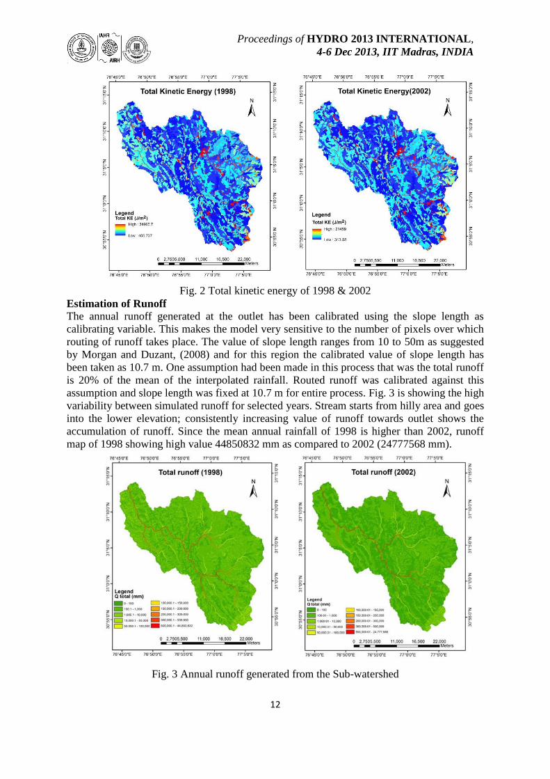
Estimation of Rainfall Energy

The total kinetic energy is a summation of kinetic energy of direct throughfall and leaf

drainage. Leaf drainage depends upon the plant height and minor change will be happen in

that with respect to time. The formula of kinetic energy discussed by Kinnell, (1981) for

tropical region is directly multiplying with the amount of direct throughfall. It means total

kinetic energy directly depends upon the amount of direct throughfall and it will change

according to rainfall received in a year. In the year of 1998 mean of interpolated rainfall was

1564 mm and for the year of 2002 it was 1098 mm, so that the high value of total kinetic

energy (Fig. 5.5) is showing 34956.7 J/m2, it is approximately 1.63 times greater than the

total kinetic energy of 2002. It shows 3.18 times higher value of actual sediment yield

estimated by model for year of 1998. It means, year which is getting high mean annual

rainfall has higher kinetic energy and this will further effect the detachment of soil particles

by raindrop impact and total sediment yield at the outlet.



12

Fig. 2 Total kinetic energy of 1998 & 2002

Estimation of Runoff

The annual runoff generated at the outlet has been calibrated using the slope length as

calibrating variable. This makes the model very sensitive to the number of pixels over which

routing of runoff takes place. The value of slope length ranges from 10 to 50m as suggested

by Morgan and Duzant, (2008) and for this region the calibrated value of slope length has

been taken as 10.7 m. One assumption had been made in this process that was the total runoff

is 20% of the mean of the interpolated rainfall. Routed runoff was calibrated against this

assumption and slope length was fixed at 10.7 m for entire process. Fig. 3 is showing the high

variability between simulated runoff for selected years. Stream starts from hilly area and goes

into the lower elevation; consistently increasing value of runoff towards outlet shows the

accumulation of runoff. Since the mean annual rainfall of 1998 is higher than 2002, runoff

map of 1998 showing high value 44850832 mm as compared to 2002 (24777568 mm).

Fig. 3 Annual runoff generated from the Sub-watershed



13

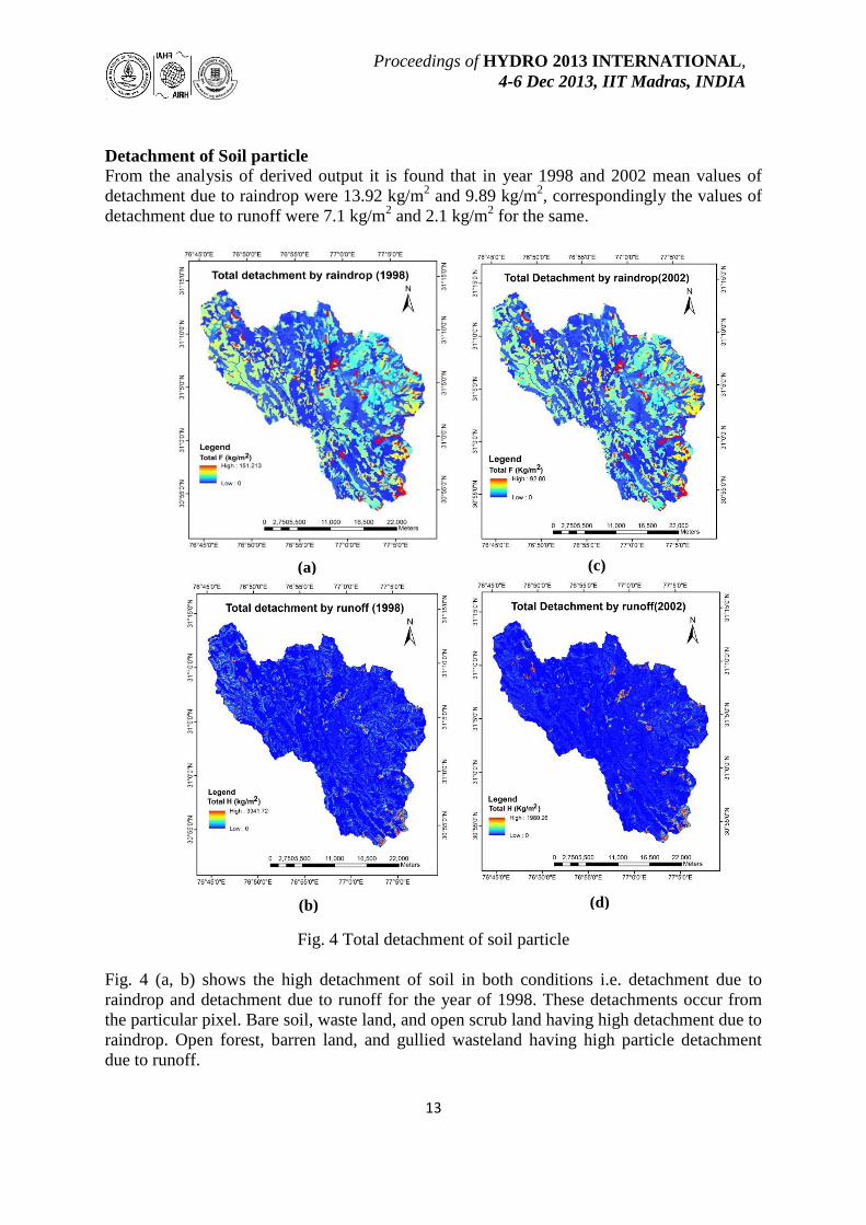
Detachment of Soil particle

From the analysis of derived output it is found that in year 1998 and 2002 mean values of

detachment due to raindrop were 13.92 kg/m2 and 9.89 kg/m

2, correspondingly the values of

detachment due to runoff were 7.1 kg/m2 and 2.1 kg/m

2 for the same.

Fig. 4 Total detachment of soil particle

Fig. 4 (a, b) shows the high detachment of soil in both conditions i.e. detachment due to

raindrop and detachment due to runoff for the year of 1998. These detachments occur from

the particular pixel. Bare soil, waste land, and open scrub land having high detachment due to

raindrop. Open forest, barren land, and gullied wasteland having high particle detachment

due to runoff.

(c) (a)

(b) (d)



14

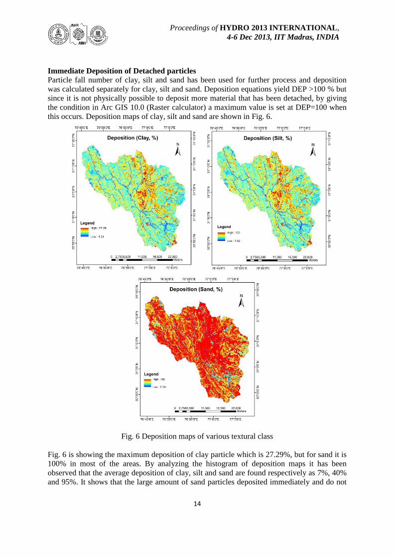
Immediate Deposition of Detached particles

Particle fall number of clay, silt and sand has been used for further process and deposition

was calculated separately for clay, silt and sand. Deposition equations yield DEP >100 % but

since it is not physically possible to deposit more material that has been detached, by giving

the condition in Arc GIS 10.0 (Raster calculator) a maximum value is set at DEP=100 when

this occurs. Deposition maps of clay, silt and sand are shown in Fig. 6.

Fig. 6 Deposition maps of various textural class

Fig. 6 is showing the maximum deposition of clay particle which is 27.29%, but for sand it is

100% in most of the areas. By analyzing the histogram of deposition maps it has been

observed that the average deposition of clay, silt and sand are found respectively as 7%, 40%

and 95%. It shows that the large amount of sand particles deposited immediately and do not



15

go for transport. In this way clay has lower deposition, silt has moderate deposition and sand

has higher deposition.

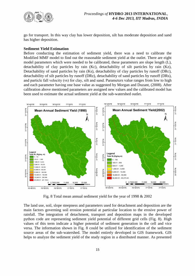
Sediment Yield Estimation

Before conducting the estimation of sediment yield, there was a need to calibrate the

Modified MMF model to find out the reasonable sediment yield at the outlet. There are eight

model parameters which were needed to be calibrated, these parameters are slope length (L),

detachability of clay particles by rain (Kc), detachability of silt particles by rain (Kz),

Detachability of sand particles by rain (Ks), detachability of clay particles by runoff (DRc),

detachability of silt particles by runoff (DRz), detachability of sand particles by runoff (DRs),

and particle fall velocity (νs) for clay, silt and sand. Parameters value ranges from low to high

and each parameter having one base value as suggested by Morgan and Duzant, (2008). After

calibration above mentioned parameters are assigned new values and the calibrated model has

been used to estimate the actual sediment yield at the sub-watershed outlet.

Fig. 8 Total mean annual sediment yield for the year of 1998 & 2002

The land use, soil, slope steepness and parameters used for detachment and deposition are the

main factors governing soil erosion potential at particular location to the erosive power of

rainfall. The integration of detachment, transport and deposition maps in the developed

python code are representing sediment yield potential of different grid cells (Fig. 8). High

values of this term indicate a higher potential of sediment generation in the cell and vice

versa. The information shown in Fig. 8 could be utilized for identification of the sediment

source areas of the sub-watershed. The model entirely developed in GIS framework. GIS

helps to analyze the sediment yield of the study region in a distributed manner. As presented



16

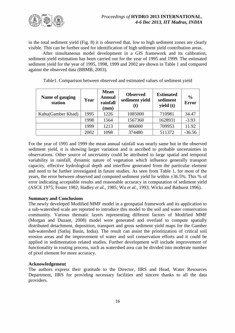
in the total sediment yield (Fig. 8) it is observed that, low to high sediment zones are clearly

visible. This can be further used for identification of high sediment yield contribution areas.

After simultaneous model development in a GIS framework and its calibration,

sediment yield estimation has been carried out for the year of 1995 and 1999. The estimated

sediment yield for the year of 1995, 1998, 1999 and 2002 are shown in Table 1 and compared

against the observed data (BBMB, 2003).

Table1. Comparison between observed and estimated values of sediment yield

Name of gauging

station Year

Mean

Annual

rainfall

(mm)

Observed

sediment yield

(t)

Estimated

sediment

yield (t)

%

Error

Kahu(Gamber Khad) 1995 1226 1085000 710981 34.47

1998 1564 1567360 1628931 -3.93

1999 1213 806000 709953 11.92

2002 1098 374480 511372 -36.56

For the year of 1995 and 1999 the mean annual rainfall was nearly same but in the observed

sediment yield, it is showing larger variation and is ascribed to probable uncertainties in

observations. Other source of uncertainty could be attributed to large spatial and temporal

variability in rainfall, dynamic nature of vegetation which influence generally transport

capacity, effective hydrological depth and interflow generated from the particular element

and need to be further investigated in future studies. As seen from Table 1, for most of the

years, the error between observed and computed sediment yield lie within ±36.5%. This % of

error indicating acceptable results and reasonable accuracy in computation of sediment yield

(ASCE 1975; Foster 1982; Hadley et al., 1985; Wu et al., 1993; Wicks and Bathurst 1996).

Summary and Conclusions

The newly developed Modified MMF model in a geospatial framework and its application to

a sub-watershed scale are reported to introduce this model to the soil and water conservation

community. Various thematic layers representing different factors of Modified MMF

(Morgan and Duzant, 2008) model were generated and overlaid to compute spatially

distributed detachment, deposition, transport and gross sediment yield maps for the Gamber

sub-watershed (Satluj Basin, India). The result can assist the prioritization of critical soil

erosion areas and the improvement of water and soil conservation efforts and it could be

applied in sedimentation related studies. Further development will include improvement of

functionality in routing process, such as watershed area can be divided into moderate number

of pixel element for more accuracy.

Acknowledgement

The authors express their gratitude to the Director, IIRS and Head, Water Resources

Department, IIRS for providing necessary facilities and sincere thanks to all the data

providers.



17

REFERENCES

Abrahams, A.D., Li G., Krishnan, C., Atkinson, J.F., 2001. A sediment transport equation for

inter rill overland flow on rough surfaces. Earth Surface Processes and Landforms 26:

1443–1459.

Arekhi, S., Shabani, A., Rostamizad, G., 2012. Application of the modified universal soil loss

equation (MUSLE) in prediction of sediment yield (Case study: Kengir Watershed,

Iran). Arabian Journal of Geosciences 5, 1259–1267.

BBMB., 2003. Sedimentation study of Bhakra Reservoir for the Year 2001-2003.

Sedimentation Survey Report, BBMB, Bhakra Dam Circle, Nangal, India.

Brandt, C.J., 1989. The size distribution of throughfall drops under vegetation canopies.

{CATENA} 16, 507 – 524.

Carson, M.A., Kirkby, M.J., 1972. Hillslope Form and Processes. Cambridge University

Press: Cambridge.

Di Stefano, C., Ferro, V., Porto, P., 2000. Length Slope Factors for applying the Revised

Universal Soil Loss Equation at Basin Scale in Southern Italy. Journal of Agricultural

Engineering Research 75, 349–364.

Gitas, I.Z., Douros, K., Minakou, C., Silleos, G.N., Karydas, C.G., 2009. Multi-temporal soil

erosion risk assessment in N. Chalkidiki using a modified usle raster model. EARSeL

eProceedings 8, 40–52.

Gosain, A.K., Rao, S., Arora, A., 2011. Climate change impact assessment of water resources

of India. Current Science(Bangalore) 101, 356–371.

Jain, M.K., Das, D., 2009. Estimation of Sediment Yield and Areas of Soil Erosion and

Deposition for Watershed Prioritization using GIS and Remote Sensing. Water

Resources Management 24, 2091–2112.

Jain, S.K., Singh, P., Seth, S.M., 2002. Assessment of sedimentation in Bhakra Reservoir in

the western Himalayan region using remotely sensed data. Hydrological Sciences

Journal 47, 203–212.

Jin, C.X., Römkens, M.J.M., Griffioen, F., 2000. Estimating Manning‟s roughness coefficient

for shallow overland flow in non-submerged vegetative filter strips. Transactions of

the American Society of Agricultural Engineers 43: 1459–1466.

Jones, A.J., Lal, R., Huggins, D.R., 1997. Soil erosion and productivity research: A regional

approach. American Journal of Alternative Agriculture 12: 185–192.

Kinnell, P.I.A., 1981. Rainfall intensity-kinetic energy relationships for soil loss prediction.

Soil Science Society of America Journal 45, 153–155.

Kinnell, P.I.A., Risse, L.M., 1998. USLE-M: Empirical modeling rainfall erosion through

runoff and sediment concentration. Soil Science Society of America Journal 62,

1667–1672.

Kirkby MJ., 1976. Hydrological slope models: the influence of climate. In Geomorphology

and Climate, Derbyshire E (ed.). Wiley: London;247–267.

Kothyari, U.C., 1996. Erosion and sedimentation problems in India. IAHS Publications-

Series of Proceedings and Reports-Intern Association Hydrological Sciences 236,

531–540.

Lal, R., 2001. Soil degradation by erosion. Land Degradation & Development 12: 519–539.

DOI: 10.1002/ldr.472.



18

Lim, J.K., Sagong, M., Engel, B.A., Tang, Z., Choi, J., Kim, K., 2005. GIS based sediment

assessment tool. Catena 64: 61–80.

Morgan, R.P.C., 1982. Stability of agricultural ecosystems : validation of a simple model for

soil erosion assessment. International Institute for Applied Systems Analysis,

Laxenburg, Austria.

Morgan, R.P.C., Quinton, J.N., Smith, R.E., Govers, G., Poesen, J.W.A., Auerswald, K.,

Chisci, G., Torri, D., Styczen, M.E., 1998. The European Soil Erosion Model

(EUROSEM): a dynamic approach for predicting sediment transport from fields and

small catchments. Earth Surface Processes and Landforms 23, 527–544.

Morgan, R.P.., 2001. A simple approach to soil loss prediction: a revised Morgan–Morgan–

Finney model. CATENA 44, 305–322.

Morgan, R.P.C., Duzant, J.H., 2008. Modified MMF (Morgan–Morgan–Finney) model for

evaluating effects of crops and vegetation cover on soil erosion. Earth Surface

Processes and Landforms 33, 90–106.

Renard, K.G., Foster, G.R., Weesies, G.A., Porter, J.P., 1991. RUSLE: Revised universal soil

loss equation. Journal of Soil and Water Conservation 46, 30–33.

SJVN (Satluj Jal Vidyut Nigam) Report, vol. 2 water& environment Satluj Jal Vidyut Nigam

Limited cumulative and induced impact assessment Rampur hydro-electric project

(RHEP) final report DHI (India) water & environment, September 2006.

Tollner, E.W., Barfield B.J., Haan C.T., Kao T.Y., 1976. Suspended sediment filtration

capacity of simulated vegetation. Transactions of the American Society of

Agricultural Engineers 19: 678–682.

Turc, L., 1961. Evaluation des besoins en eau d‟irrigation, evapo-transpiration potentielle,

formule climatique simplifieetmise á jour. Annales Agronomie 12: 13–49.

Ustun, B., 2008. Soil erosion modelling by using GIS and remote sensing: a case study Ganos

Mountain. The international archives of the photogrammetry, remote sensing and

spatial information sciences 37, 1681–1684.

Xu, Y., Shao, X., Kong, X., Peng, J., Cai, Y., 2008. Adapting the RUSLE and GIS to model

soil erosion risk in a mountains karst watershed, Guizhou Province, China.

Environmental Monitoring and Assessment 141: 275–286. DOI: 10.1007/s10661-007-

9894-9.

SEDIMENT YIELD ESTIMATION USING MODIFIED MMF MODEL IN A GEOSPATIAL ENVIRONMENT

Documents

Transcript of SEDIMENT YIELD ESTIMATION USING MODIFIED MMF MODEL IN A GEOSPATIAL ENVIRONMENT