SDVS 11 Users' Manual - DTIC
348
SDVS 11 Users' Manual 30 September 1992 Prepared by L. G. MARCUS Computer Systems Division AEROSPACE REPORT NO. ATR-92(2778)-8 Prepared for NATIONAL SECURITY AGENCY Ft. George G. Meade, MD 20755-6000 Engineering and Technology Group pfenaBUfl fKKl 19950302 069 CORPORATION El Segundo, California PUBLIC RELEASE IS AUTHORIZED
-
Upload
khangminh22 -
Category
Documents
-
view
0 -
download
0
Transcript of SDVS 11 Users' Manual - DTIC

SDVS 11 Users' Manual
30 September 1992
Prepared by
L. G. MARCUS Computer Systems Division
AEROSPACE REPORT NO. ATR-92(2778)-8
Prepared for
NATIONAL SECURITY AGENCY Ft. George G. Meade, MD 20755-6000
Engineering and Technology Group
■pfenaBUfl fKKl
19950302 069
CORPORATION El Segundo, California
PUBLIC RELEASE IS AUTHORIZED

Aerospace Report No. ATR-92(2778)-8
SDVS 11 USERS' MANUAL
Prepared by
L. G. Marcus Computer Systems Division
30 September 1992
Engineering and Technology Group THE AEROSPACE CORPORATION
El Segundo, CA 90245-4691
Prepared for
NATIONAL SECURITY AGENCY Ft. George G. Meade, MD 20755-6000
PUBLIC RELEASE IS AUTHORIZED

SDVS 11 USERS' MANUAL
Prepared
L. G. Marcus
Approved
Report No. ATR-92(2778)-8
B. H. Levy, Manager ^ Computer Assurance Section
xh^ D. B. Baker, Director Trusted Computer Systems Department
C. A. Sunshine, Pri Computer Science
Subdivision
icjpal Director id Technology
ni
Accession 7or
HTIS GRA&I DTIC IAB Unannounced Justification.
D D
By _^
Availability OCdes
Bist. ivail and/br
Special

Abstract
This is a guide for users of SDVS, Version 11. Its style is somewhere between that of a tutorial and a reference manual.
All facets of the verification system are covered here: the underlying logic (state deltas), the proof language, the user interface, the actual use of the system, the translation from the register-transfer-level language ISPS to state deltas, the translation from Ada to state deltas, the translation from VHDL to state deltas, the capabilities of the static solvers, and example proofs. In addition, a set of exercises is provided in the last chapter.

Acknowledgments
The author gratefully acknowledges the other members of the Computer Verification Project: Mark Bouler, John Doner, Ivan Filippenko, Beth Levy, Dave Martin, Telis Menas, and David Schulenburg; and members of the editorial staff, Melodee Lydon and Mike Meyer, for their substantial contributions to this manual.
VI

Contents
Abstract v
Acknowledgments vi
1 INTRODUCTION 1
1.1 PRELUDE 1
1.2 OVERVIEW 2
1.3 INSTALLING SDVS 5
1.4 STATE DELTAS 8
1.4.1 Expressing a Computation as a State Delta 8
1.4.2 Expressing a Claim about a Computation as a State Delta 11
1.4.3 Assuming and Proving a State Delta 12
1.5 THE MODEL OF STORAGE 12
1.6 THE STRUCTURE OF SDVS 14
1.7 INPUTTING THEOREMS 16
1.8 GETTING AROUND IN SDVS 16
1.9 SOME PRACTICE ON THE SYSTEM 17
1.10 SYSTEM HELP 22
2 THE PROOF LANGUAGE 41
2.1 A DYNAMIC EXAMPLE 41
2.2 STARTING AND ENDING A PROOF 46
2.3 STRAIGHT-LINE SYMBOLIC EXECUTION 47
2.4 PROOF BY CASES 49
2.5 PROOF BY INDUCTION 54
2.6 PROOF BY CONTRADICTION 61
2.7 STATIC PROOF 65
2.7.1 Axioms 66
2.7.2 Rewriting 69
vu

2.7.3 Current Axiom List 71
2.7.4 Lemmas 80
2.7.5 Notice 86
2.7.6 Solvers 87
2.8 MANIPULATING THE PROOF 89
2.8.1 Defer 89
2.8.2 Pop 93
2.8.3 Stop and Continue 94
2.9 MISCELLANEOUS 95
2.9.1 Flags 95
2.9.2 Queries 96
2.9.3 Introduction of Constants 103
2.9.4 Declarations 104
2.9.5 Data and Array Allocation 106
2.9.6 Negate 109
2.9.7 Linearize 114
2.9.8 Natural Number Induction 118
2.9.9 Mapping , 119
2.9.10 Formulas 125
2.9.11 Macros 128
2.9.12 Composition of State Deltas 129
2.9.13 The SDVS Language Parser 132
2.9.14 Reading, Writing, and Editing 135
2.9.15 Batch Proofs 137
2.9.16 Disjunctions of State Deltas 138
2.9.17 System Commands 139
2.9.18 Errors 139
2.9.19 Breaks in SDVS 140
2.9.20 Bugs in SDVS 140
vm

3 INTERACTION WITH ISPS 143
3.1 TR: TRANSLATOR FROM ISPS TO STATE DELTAS 143
3.2 MARKING 145
3.3 EXTENSIONS OF ISPS 150
3.3.1 Extending ISPS by Assumptions and State Deltas 150
3.3.2 External and Auxiliary Variables 156
3.3.3 External Variables 156
3.3.4 Auxiliary Variables 159
3.4 THE NEW ISPS TRANSLATOR 162
4 INTERACTION WITH ADA 165
4.1 TR: TRANSLATOR FROM ADA TO STATE DELTAS 166
4.1.1 Ada Language Subsets 166
4.1.2 SDVS 11 Ada Language Features 166
4.2 COMMANDS DEALING WITH ADA 167
4.2.1 Theorems 168
4.2.2 Input and Output 169
4.2.3 Proof Strategy 169
4.3 EASY EXAMPLE OF AN ADA PROOF 171
4.4 N0NTRD7IAL EXAMPLE OF AN ADA PROOF 177
4.5 OFFLINE CHARACTERIZATION 181
4.6 AN EXAMPLE PROOF WITH ADALEMMA 197
5 INTERACTION WITH VHDL 207
5.1 INTRODUCTION 207
5.2 STAGE 2 VHDL 208
5.3 TRANSLATION OF STAGE 2 VHDL 212
5.4 AN EXAMPLE 213
6 QUANTIFICATION 231
6.1 QUANTIFICATION PROOF COMMANDS 232
IX

6.1.1 Quantification 232
6.1.2 Usablequantifiers 233
6.1.3 Enotice 233
6.1.4 Instantiate 235
6.1.5 Provebygeneralization 237
6.1.6 Provebyinstantiation 238
6.1.7 Makeboundedquantifier 242
6.1.8 Quantification Axioms 244
6.1.9 Quantification Flags 247
6.2 PROOF OF A SORT PROGRAM 247
7 USER-DEFINED DATA TYPES 257
7.1 INTRODUCTION 257
7.2 SDVS COMMANDS 259
8 INVARIANTS IN SDVS 261
8.1 NOTICEINVARIANT 263
8.2 LINEARIZE 265
8.3 NOTICECONCURRENTSD 274
8.4 NEGATE 278
8.5 OMEGAINDUCT 281
9 THE SIMPLIFIER 289
9.1 PROPOSITIONS 290
9.2 EQUALITY 291
9.3 ARITHMETIC 293
9.3.1 Linear Integer Arithmetic 295
9.3.2 Integer Multiplication 296
9.3.3 Integer Division, Remainder, Modulus, and Absolute Value 298
9.3.4 Integer Exponentiation 299
9.4 BITSTRINGS 302

9.5 ARRAYS 306
9.6 COVERINGS 310
9.7 LISTS 317
9.8 QUEUES 317
9.9 ENUMERATION TYPES 319
9.10 VHDL TIME 321
9.11 VHDL WAVEFORMS 322
10 SDVS EXERCISES 325
References 329
XI

1 INTRODUCTION
1.1 PRELUDE
This manual is intended for users of the State Delta Verification System Version 11 (SDVS 11). It is a blend of a reference manual and a tutorial. This version of the manual supersedes the previous manual [1], which described SDVS 10, although much of the text is common to both. The SDVS tutorial [2] contains additional examples and explanations.
Other easily accessible published background material on SDVS can be found in [3], [4], and [6]. References for further information on SDVS are to be found in the SDVS bibliography at the end of this manual.
SDVS is written in Common Lisp. It currently runs in Lucid Common Lisp 4.0 and Franz Allegro Common Lisp 4.1. SDVS can be run directly in Lisp, but it is preferable to run SDVS from GNU Emacs, which then gives the user editing capabilities.
SDVS 11 is for the most part upwardly compatible with all previous version of SDVS. The main improvements of SDVS 11 over SDVS 10 are the following:
• A capability to translate Ada programs containing "FOR" loops (Section 4.1.2).
• A capability to translate VHDL descriptions with (restricted) design files, declara- tive parts in entity declarations, package STANDARD (containing predefined types BOOLEAN, BIT, INTEGER, TIME, CHARACTER, REAL, STRING, and BIT-VECTOR), user-defined packages, USE clauses, array type declarations, enumeration types, sub- programs (procedures and functions, excluding parameters of object class SIGNAL), concurrent signal assignment statements, FOR loops, octal and hexadecimal represen- tations of bitstrings, ports of default object class SIGNAL, and general expressions of type TIME in AFTER clauses (Section 5).
• The VHDL and Ada translators have been reengineered to a uniform implementation reflecting language similarities where they exist, and optimized for greater space- and time-efficiency.
• The new proof command omegainduct (Section 8.5).
• The new flags strongcoverings (Section 2.9.1) and weaknextJr (Section 4).
• A capability to "read" and "write" adalemmas (Section 2.9.14).
• Several UNIX1-type commands: exit, shell, cd, pwd (Section 2.9.17).
This introductory chapter will be sufficient to let the user get started on the system. Other chapters detail the following aspects of the theory and operation of SDVS 11:
^NIX is a trademark of Bell Laboratories.

1. the internal logic (state deltas) (Chapter 1)
2. the proof language (Chapter 2)
3. the user interface (throughout)
4. actual system use (throughout)
5. the translation from the hardware description language ISPS to state deltas (Chap- ter 3)
6. the handling of quantification (Chapter 6)
7. user-defined data types (Chapter 7)
8. the invariant extension to state deltas (Chapter 8)
9. the translation from a subset of the programming language Ada to state deltas (Chap- ter 4)
10. the translation from a subset of the hardware description language VHDL to state deltas (Chapter 5)
11. the capabilities of the static solvers (Chapter 9)
12. example proofs (throughout)
13. exercises (Chapter 10)
A word about the index at the end of this manual: command names are listed under "Command-name" as well as individually.
Before one begins the significant effort involved in learning to use a verification system such as SDVS, he or she should certainly be aware that the utility of verification, or the role that verification plays in providing confidence in computer systems, is an important issue. We assume that the potential user is either already aware of the value of verification, or at least believes in the possibility of such value. For a strong, if sometimes overstated, argument in favor of verification, we recommend [7].
1.2 OVERVIEW
The State Delta Verification System, SDVS, is a system for checking proofs about the course of a computation, usually called "correctness" proofs. SDVS can be used to check microcode implementation correctness proofs, program verification proofs (e.g. liveness and safety for Ada programs), or hardware correctness proofs (e.g. liveness and safety for VHDL hardware descriptions). As a test of the system's microcode correctness capabilities, SDVS 5 was used to analyze most of the instruction set of the BBN C/30 computer. A summary of that work is presented in [8].

In SDVS 11, the theorems to be proved for the above cases of program and hardware correctness must still be explicitly written by the user in the internal logic of state deltas. However, beginning with SDVS 6, if the user is interested in proving implementation or microcode correctness theorems, SDVS will construct the theorem automatically, given the relevant information; i.e., the system can be instructed to prompt the user for
1. the descriptions of a host machine (often microprogrammed) and target machine writ- ten in either a somewhat extended subset of the machine description language ISPS, or the internal SDVS state delta language;
2. the microcode (if any);
3. the correspondence between the program variables (machine places) in the host and target; and
4. the proof of correctness that the host implements the target with respect to the correspondence (if such a proof is already constructed.)
SDVS then automatically constructs the state delta representing the theorem of correctness of the implementation, and either checks the proof, if one was given in step 4 above, or allows the user to construct one interactively.
The user communicates to SDVS through several languages. The proof language is used to write the proof that the system will check. The state delta language is used to write the theorems to be proved and to describe the relevant programs and specifications. The user-interface language allows for interactive proof building, querying, and so on. Finally, there is a module that translates from a subset of ISPS ([9], [10]), from a subset of Ada ([11] - [20]), and from a subset of the hardware description language VHDL ([21] - [27]) into state deltas.
Recently, the underlying logic has been enhanced to allow for the specification of (state- transition) invariants. For more background on the use of invariants in state deltas, consult [28]'- [32].
Technically, SDVS aids in the writing and checking of proofs of state deltas. For example, state deltas can specify claims of the form "If P is true now, then Q will become true in the future." If P is (the translation of) a program (perhaps with some initial conditions) and Q is an output condition, then the above claim is an input-output assertion about P. SDVS can also specify (and prove) claims of the form ';If P is true now, then Q is true now." In this case, if P is a (state delta representing a) program or hardware description and Q is a (state delta representing a) specification, then the above claim asserts the implementation correctness of P with respect to Q.
Finally, SDVS can prove claims of the form "If P is true now, then Q will always be true in the future," or until some other condition becomes true.
The view of the world captured by state deltas is that there are "places" (to be thought of as abstract machine registers, usually called program variables in other contexts) that can

"hold" contents. A "state" of a computation or a machine is, to first approximation, an association of contents with places. In general, a set of states can be specified by any set of sentences that relate the contents of some places with the contents of other places. For example, the sentence .x > 5 can be thought of as specifying the set of states in which the current contents of x are greater than or equal to 5, with no restriction on any other places that happen to "exist."
The "if-now, then-later" statement above is the basic building block of state deltas. It can be thought of as a specification of a state change, with P being the "precondition" (the condition allowing the state change to occur) and Q the "postcondition" (the description of the state after the change has occurred). A sequential computation is thought of as a sequence of state changes; as we will see, there are several ways in which such a sequence of state changes can be specified by a state delta or set of state deltas. The word "delta" indicates our intention to describe "small" state changes, those state changes in which only a small part of a large state is changing. In order to specify the resultant state after the change, instead of listing all true facts, it would be much more efficient simply to list those places that have (or possibly have) changed during the transition. Typically this will be a small list, called the "modification" list. The true statements at the end of the transition are those explicitly given in Q, plus those statements true in the precondition state that involve variables that do not appear in the modification list. In particular, if it is specified that no variables are allowed to change as the state changes from P to Q (the modification list is empty), and Q is a first-order sentence, then Q must be true in the state that satisfies P, and we are simply looking at the static claim that P implies Q.
The proof language can be divided into two parts, the dynamic and the static. The dynamic part controls the state transitions made by the system. There are constructs for proof by symbolic execution for straight-line code, proof by cases for branching code, and proof by induction for loops. In addition, there are several more-specialized proof commands, such as the command to sequentialize two simultaneously true state deltas. Of course, when the execution has arrived at a new state, a static proof may be needed to verify that new relations do in fact hold, i.e., they follow from the facts known explicitly about the new state (in order to show that the postcondition is true and the goal is reached, or to show that a precondition is true and a new state delta may be applied; see below).
The static part of the proof language deals with proving that certain assumptions imply certain conclusions about a given state. For simple domains where efficient decision proce- dures exist and are implemented, the system will be able to derive all conclusions without any user-input proof. Examples are equality over uninterpreted function symbols, a frag- ment of naive set theory, and linear arithmetic. For more complicated domains, our current philosophy and implementation allow the user to write proofs by having the system notice incrementally more difficult conclusions, where the newly verified conclusions are stored and used as facts on which to base the next conclusion. The derivation from a given set of facts to the next conclusion may be automatic in some cases, or it may require the user to designate that an axiom or a previously proved lemma is to be applied.
SDVS may be run in interactive mode, batch mode, or, as in most real applications, as a combination of the two. In interactive mode the user writes the proof in SDVS with

help from system prompts, with the system executing each proof command as it is written. Expressions are written in standard infix notation (e.g. x+y). In batch mode the proof is written either by the SDVS dump-proof and write command, or in an editor, and then is executed in SDVS with no further user interaction. Most commonly, a partial proof is written interactively, stored, and then rerun in batch mode at a later time when the proof-writing process is being continued.
(Technical note: currently some proofs can be rerun only in a new SDVS session. This is the case when names of formulas are created during the proof. The system does not currently allow names to be reused without the user explicitly and interactively validating such an action. Since the name appearing in the proof will already have been used, the proof will abort at that point. Such a proof is the example on page 115 using the command linearize.)
The most important property of a proof-checker is that it should not allow invalid proofs to be accepted. Nevertheless, there is a trade-off. Our philosophy has been to protect the benign user from inadvertently proving falsehoods; we do not guarantee that a scheming and knowledgeable user will be unable to do so intentionally. Thus, no absolute guarantee should be attached to a proof, just because it comes out of an SDVS run with a "QED" certificate.
An example of this trade-off comes in the use of lemmas stored in a file. It is of course possible for users to change the statement of a lemma or its proof in an editor inadvertently. Thus we have provided a means for users to protect themselves against this possibility, if they so desire, by having the proof of a lemma rerun as the lemma is read into SDVS before it is actually used. But for efficiency's sake, we do not require that this be done.
Another example of the lack of total soundness is that it is possible, through self-referencing state deltas, to prove a contradiction. We have not gone to the trouble of eliminating this loophole (although we know how: see [33]), because under "normal" circumstances a user would not employ explicit self-reference. See Section 2.9.19 for an example.
1.3 INSTALLING SDVS
SDVS is available on magnetic tape in four different formats: source code; object code for Franz Allegro Common Lisp (FACL); object code for Lucid Common Lisp (LCL); and as a standalone executable utilizing the Franz Allegro Runtime package. Each format requires its own procedure for creating or loading SDVS, as outlined below. However, the procedure for reading the system files from the tape is the same for all formats.
SOFTWARE REQUIREMENTS
SDVS currently runs under Franz Allegro Common Lisp release 4.1 and Lucid Common Lisp 4.1. SDVS is also available as a standalone executable utilizing the Franz Allegro Runtime package; users of this version of SDVS are riot required to supply their own Common Lisp environment.

Table 1: Disk Space Requirements for SDVS 11
To Load From Tape Installed Source (.lisp) 2.4 N/A Lucid Object (.sbin) 2.7 31.5 Franz Object (.fasl) 3.7 48.1 Franz Runtime 8.9 38.9
DISK SPACE REQUIREMENTS
Table 1 gives the disk space requirements for SDVS 11. "Installed" represents the disk requirements of the system after SDVS has been installed, and assumes that the tar archive has been recompressed. The size of your installed executable image, if you are building SDVS from the source or either binary version, will depend on the size of your (vanilla) Common Lisp image. These numbers are therefore approximate. All numbers are in mega- bytes (MB).
READING THE SYSTEM FILES
First, you should create a top-level directory to contain all of the files and subdirectories associated with SDVS. In our system, this directory is called versys (for VERification SYS- tem) and resides as a subdirectory under /u giving /u/versys. Although you can give your directory any name, we suggest you use the same name for compatibility; yours can be located anywhere, however. For example, you might put it as a subdirectory of /usr/lib, giving /usr/lib/versys. For the examples below, we assume you have /usr/lib/versys as your top-level directory.
Next, you will want to load the SDVS system tar file from the tape. To do this, create a tmp directory in your top-level versys directory, connect (cd) to it, and extract (tar) the system tar file as follows ([unix] is the system prompt):
[unix] tar xfmv xxx
where xxx is the device name for your tape drive, e.g. /dev/rstO. This will create a file named sdvsnn-xxxx. tax .Z where nn is the current release number (e.g. 11) and xxxx is lisp (for source files), sbin (for LCL object), fasl (for FACL object), or runtime for FACL Runtime. The file is compressed, so it must be uncompressed:
[unix] uncompress sdvsnn-xxxx.tar
replacing nn and xxxx appropriately.
Now, the system directories must be extracted from the tar file:
[unix] tar xfmv sdvsnn-xxxx.tar
This process creates a file structure containing the individual files from which the SDVS system can be used or built. Once this process is complete, you may delete sdvsnn-xxxx. tax

if you feel you have no further need for it. An alternative is to recompress the file. Both will save disk space.
[unix] compress sdvsnn-xxxx.tar
Before you can build and use an SDVS executable image or use the FACL Runtime exe- cutable, you must define a UNIX environment variable as follows. This can be done directly in the shell in which you plan to build or use SDVS or by adding the command to your . cshrc file.
[unix] setenv SDVS-DIR "/usr/lib/versys/"
Of course, you will need to supply the correct path you have chosen for your top-level directory. Please note the slash (/) character at the end; it is required.
BUILDING AN SDVS EXECUTABLE IMAGE
Once you have all of the system files available, you can build an executable SDVS image. To do this, you must start up a (vanilla) Common Lisp session (either LCL or FACL) and load the init-sdvs.lisp file found in your top-level directory. (If you don't know how to start up a Common Lisp session, see your system administrator.) For example, to load the file, type
> (load "/usr/lib/versys/init-sdvs")
After the init-sdvs.lisp file has been loaded, you are ready to tell Lisp to build your SDVS executable. Two functions will do this: make-sdvs builds from the object files; make-new- sdvs builds from the source files and compiles the entire system. Each function takes one argument, the name you wish to give the executable; the executable will automatically reside in your top-level directory. You may give the executable any name you want; in the following examples, we use the name sdvsll for our executable. Each of these functions will produce a trace of what is happening. (NOTE: For these operations, you must have write privileges to the appropriate directories.)
For creating an SDVS executable from source:
> (make-new-sdvs "sdvsll")
For creating an SDVS executable from binary:
> (make-sdvs "sdvsll")
You may safely ignore any warning message printed by the system. When you return to the Lisp prompt, you can exit Lisp by
> (quit)
USING THE SDVS RUNTIME EXECUTABLE
If you have extracted the SDVS system files from a tape containing the "runtime" format, the file /usr/lib/versys/sdvsll (assuming the appropriate top-level directory) contains the executable image. This can be used to run SDVS directly, as noted below.

RUNNING SDVS
You have gone through this procedure and have created your executable. How do you run SDVS? At the Unix shell, just type, for example
[unix] /usr/lib/versys/sdvsl 1
or just sdvsll if you are connected (cd) to the top-level directory (/usr/lib/versys in our example) or if your SPÄTH environment variable contains the path to the top-level directory.
RUNNING THE TEST SUITE
Included in the SDVS release is a set of tests that exercise the system. To run these tests, you must first start up SDVS. (After building your SDVS executable, you should restart SDVS so that the system is initialized properly.) When you get to the SDVS prompt, you will want to evaluate the expression, invoking the tests as follows:
<sdvs.i> eval expression: (run-sdvs-test-proofs)
A very long trace will appear. If the tests run successfully (this may take over two hours on a Sun 4), you will return to the SDVS prompt. H something goes wrong, Lisp will "break," allowing you to examine the system; Lisp will print out some diagnostic information and put you at a prompt. If this should happen, you may exit Lisp by typing (quit).
You may restart SDVS by first returning to the top level of Lisp and invoking the function sdvs as follows:
> (sdvs)
From the SDVS prompt, you can return to Lisp by typing the SDVS command bye.
1.4 STATE DELTAS
In this section we gradually lead up to the full definition of (standard) state deltas, which appears on page 11. State deltas with invariants are defined in Chapter 8. We adopt an outlook that sees a duality between programs and certain kinds of theories (collections of facts), in the sense that a program (a set of computations) can be seen as the set of all (temporal) facts that hold in all its computations, and a computational theory can be seen as the set of all possible computations the theory allows. For a fuller discussion, see [341 or [35].
1.4.1 Expressing a Computation as a State Delta
A state delta is a description of a transition from one state to another. For example,
[sd pre: (.a = 1) post: (#b = 2)]

where sd indicates that this is a state delta formula, pre: is the precondtion field, post: is the postcondition field, a and b are places, the dot (.) is the function symbol for "contents of" before the transition, and the pound (#) is the function symbol for "contents of" after the transition. We have temporarily left out two more fields, the comodification list (comod:) and modification list (mod:) fields. This incomplete state delta represents the transition from the precondition, a state in which the contents of a are 1, to the postcondition, a state in which the contents of b are 2; that is, if at any time .a=l, then there will be a later time when #b=2. (Note that there is no specification as to when this later time is.) The modification field (mod:) will list those places that are allowed to change between the precondition and postcondition times. One possibility is that a given place does not change, or that stich a change is irrelevant. However, it could be that the system described has some interrelationships that imply that when b gets the value 2 as indicated above, b or some other places may in fact change, or have to change, but the user is either unaware of or uninterested in what those changes are. A mechanism is needed that allows the expression of the fact that during a transition, certain places may have changed their contents, i.e., that the contents of those places cannot be assumed to remain the same. More generally, any sentence dependent on those places that change cannot be assumed to be preserved during such a transition.
The problem is solved by including in a state delta an explicit list of the places that are not guaranteed to preserve their contents, or that may have their contents modified. Thus the above state delta could become
[sd pre: (.a = 1) mod: (a,b,c) post: (#b = 2)]
This means that from a state in which the contents of a are 1, we will get to a state in which the contents of b are 2, and in this transition all places, except perhaps a, 6, and c, preserve their contents. Thus, a state delta with an empty mod list encodes a static claim, i.e., a claim about a transition in which nothing changes, and thus, if first-order, a claim about the current state.
If one wanted to encode the assignment statement a := a + 1 as a state delta, it would be, to first approximation,
[sd pre: (true) mod: (a) post: (#a = .a + 1)]
If a were not in the mod list above, the resulting state delta woidd be inconsistent, that is, it could never be realized by a real computation, since a could not be replaced by a + 1 without a being allowed to change value. We currently do not allow pounds (#) to appear in the precondition.2 A dotted place in the postcondition refers to the contents of that place at the time the precondition is checked.
2 Although this change is not planned, we could interpret pounds in the precondition to refer to precon- dition time, as dots do now, and then interpret dots to refer to the time at which the state delta became true.

The last ingredient of basic (i.e., without invariant list) state deltas, the comodification list, is used to regulate how long a usable state delta remains usable. It helps to consider the following intuition behind state deltas: state deltas describe various computations, and the validity or accessibility of those descriptions changes (possibly) as a function of time. For example, one may think of state deltas as processes that may be "activated" at one time and "deactivated" at other times. So in order to specify that the assignment statement a := a +1 will be applied only once (not repeatedly as in a loop), and then will be no longer accessible, the state delta will have to be
[sd pre: (true) comod: (a) nod: (a) post: (#a = .a + 1)]
or possibly
[sd pre: (true) comod: (pc) mod: (a,pc) post: (#a = .a + 1)]
where pc (program counter) is some new place. As long as the places in the comodification list do not change values, a usable state delta will remain usable and thus applicable at any time its precondition is true. So for the above state deltas, once either is applied it may not be reapplied, since the mod list and the comod list intersect. Note that this result holds simply because of the intersection, not because any places actually change value, a fact that, in some cases, we may never know. SDVS, for the sake of soundness, must take the conservative position that established facts will go away, unless we can prove that they remain. This is to be contrasted with the "default reasoning" position that established facts will stick around, unless we have good reason to believe that they should go away.
To continue with the intuition behind the comod list, consider a supply of state deltas, each of which is introduced at a certain time, and each of which must have its precondition become true in order to "execute" (or be "applied") and bring about its postcondition. It could be the case that for a certain state delta to be applicable, most of the state at the time of its introduction must be unchanged except for one condition that is stated in the precondition. In order not to have to list all state characteristics that must remain in force, one can list those places that must remain unchanged since the time of the state delta's introduction in order for that state delta to be applicable. This is the comodification list. If one of those places changes before the precondition becomes true, the state delta cannot become applicable and is removed from the supply. (Of course, it can be explicitly introduced again in the future.) So, the following state delta
[sd pre: (.a gt 0) mod: (a) post: (#a = .a + 1)]
is true at a certain time ("now"), if at any time in the future (from then) when the contents of a are greater than 0, there is a (not necessarily strictly) later time at which the contents of a will be incremented by 1, and nothing else would have changed. However, at this later time the contents of a are still greater than 0, and so the state delta is "reapplicable." In other words, there is a still later time at which the contents of a are further incremented, and the process can be continued ad infinitum.
The state delta
10

[sd pre: (.a gt 0) comod: (a) mod: (a) post: (#a = .a + 1)]
is true "now" if at any later time at which the contents of a are greater than 0, and in the interval between now and that time the contents of a have not changed (a is in the comodification list), then there is a (not necessarily strictly) later time at which the contents of a are incremented by 1 and nothing has changed except the contents of a (only a is in the modification list). The truth of this state delta now does not imply that it will still be true at the time when the contents of a are actually incremented, because the comodification list will have changed. Note that a true state delta with an empty comodification list will be true at any time in the future.
The general definition follows.
Definition: Let p and qbe lists of first-order sentences or previously defined state deltas (an implicit conjunction), where the first-order sentences in p and in the preconditions of any state deltas embedded within p and q are #-free, and let c and m be lists of places. The state delta
[sd pre: (p) comod: (c) mod: (m) post: (q)]
is true at time to in a given computation if at any later ii > to at which p is true and the contents of the places in c have not changed between to and ti, then there is some still later time 22 > *i in the computation at which q is true and only the contents of the places in m may have changed between t\ and 22 •
The extra invariant (inv:) field is discussed in Chapter 8.
1.4.2 Expressing a Claim about a Computation as a State Delta
Much added expressive power comes from allowing the precondition and postcondition themselves to contain state deltas in addition to first-order sentences. This is well-defined, since all one must do is evaluate the truth of the precondition and postcondition at certain times, and this evaluation can be done for state deltas as well as for "static" sentences.
Thus the following is a true state delta:
[sd pre: (.a = 1, [sd pre: (.a gt 0)
mod: (a) post: (#a = .a + 1)])
mod: (a) post: (#a = 1000)]
This state delta can be interpreted as a claim about the computation represented by the state delta (call it S) embedded in the precondition; i.e., if the contents of a are 1 and S is constantly active, then definitely at some future time the contents of a will be 1000. Note that the above does not determine anything else about the values of a (for example, that
11

a increases monotonically). Intermingled between the times when a takes on the values 1, 2, ..., 1000, ..., a can take on arbitrary values. Also, nothing is specified about the length of the time interval between these increasing values, nor about how long these values are maintained once they are achieved.
1.4.3 Assuming and Proving a State Delta
First, we want to clarify several terms relating to state deltas that have been found to be confusing to users of SDVS. They are: "true state delta," "usable state delta," and "applcable state delta." A true, or valid, state delta is one which holds in every computation according to the semantics given on page 11. Every state delta theorem proved in SDVS, i.e., proved at the top level, is (we hope) a true state delta. A usable state delta is one which is known by SDVS to be true at the current time in the current context, i.e., is in the list of usablesds. An applicable state delta is a usable state delta that can be applied in the current context, i.e., whose precondition is true. After it is applied, it may remain applicable, usable, or neither in the new state.
In order to prove the above state delta, i.e., that it is true "now," SDVS assumes there is a later time at which the precondition is true and the contents of the places in the comodi- fication list (there are no such places in this example) have not changed. The precondition consisting of the first-order sentence about a and the state delta S is stored in a database representation of the "current state" of the computation. Then one shows, in this case by direct execution or induction, that there exists a state in which the postcondition becomes true.
For the sake of simplicity, we now describe a step of the symbolic execution proof. (Induction will be discussed in Section 2.5.) The fact that S is in the current state (i.e., true) allows a state transition to take place. The precondition of S, .agtO, is also true in the current state, so one may advance the state to the time of S's postcondition, #a= .a + 1. Now one must update the current state. It contains the fact that the contents of a are now 2. How about S? S has an empty comodincation list also, so it will be true at any time after the original "now." Thus S also belongs to the new current state. Since the precondition of S is still true, S may be reapplied, which brings about the state where the contents of a are 3. This process can obviously be continued until the contents of a become 1000. One final check is needed to prove the state delta: it must be verified that the postcondition was achieved within the constraints of the modification list. Indeed this is so: since the modification list of S contained only a, the whole computation involved only changes in a.
1.5 THE MODEL OF STORAGE
There is one additional element of the state delta paradigm that we have not yet considered, the dependence relations among the places. The covering predicate represents architectural information about the "overlap" of places, and is needed in processing the comod and mod lists in order to update the state. Without an explicit covering statement mentioning all
12

places in a given state delta, SDVS may behave too conservatively. If there is no overlap among places, that has to be explicitly stated.
For example, if b is in the modification list of a state delta, that means that b is allowed to change when that state delta is applied, and thus, we cannot know a priori (i.e., based on the previous value of b) what it's new value will be. The contents of b must be explicitly updated at postcondition time (either in accordance with the information in the postcondition about b, or simply to "don't know"). If a happens to be defined as the concatenation of b with c, say, then a must also be similarly updated at postcondition time. In this case, or in the more general case of a being the disjoint union of b and c, one would write COVERING (A, B, C).J£ the user has knowledge that is more explicit (e.g. that a is the concatenation of b and c), those details would have to be specified separately, and then of course further information about the relation among the values of a, 6, and c could be deduced.
Think of covering(place, subplace1, subplace2,..., subplacen)
as representing the condition that place is the disjoint union of {subplace1, subplace2,..., subplacen}. [Note to advanced SDVS users: to model more general situations, think of
covering(place, subplacel, subplace2, ■ ■ ■, subplacen)
as representing the condition that {subplace-^, subplace2, ■ ■., subplacen} is a minimal inde- pendent set suchthat the value of place is a function of (.subplace1: .subplace2,..., .subplacen). But we will not get into the technical details here.] In particular, if place is actually the dis- joint union of the mentioned subplaces, and the contents are calculated by concatenating the contents of the subplaces, then certainly the above covering relation holds. Thus, a change in .place means that there was a change in at least one of .subplace1, .subplace2,..., .subplacen; therefore, unless we know more specifics, we must assume all have potentially changed value. Similarly, unless we know otherwise, a change in the value of one of the subplaces means we must assume that .place changed. Note that we do not insist that the value of place be a one-one function of {.subplace^ .subplace2,..., .subplacen); thus, the value of a sub- place may change without the value of place actually changing. However, in cases where we do want to enforce that the function be one-one, we have the strongcoverings flag (see Section 2.9.1).
Thus, under the hypothesis that covering(all, a, b) (all represents the set of all places) and covering(a, c, d) hold, the following state delta is inconsistent:
SI:
[sd pre: (true) mod: (d) post: (#c = .c + 1)]
while the following are consistent:
S2:
[sd■pre: (true) mod: (c)
post: (#c = .c + l,#a = .a)]
13

S3:
[sd pre: (true) mod: (b,c) post: (#a = .a,#b = 1)]
S4:
[sd pre: (true) mod: (c) post: (#a = .a + 1)]
(To see how the system responds to the hypothesis of an inconsistent state delta, see Section 2.6.) To see why S2 is consistent, we must use the abstract dependency interpretation of coverings. For example, assuming that covering(a, c, d) means that a depends on c and d, but c and d are independent, we can consider the situation in which .a = .c + .d if .c < 5, and .a = 5 + .d otherwise. Then .c can go from 5 to 6 without changing the value of a. S3 is similar: in S3 the contents of d are not allowed to change during the computation, since d does not appear in the mod list, a does not have to appear in the mod list, even though its contents may have changed during the computation (as a result of the fact that c is in the mod list). If c had been omitted in the mod list and #6=1 had been omitted in the postcondition, then the resulting state delta would have been true (and provable in SDVS).
S4 is seen to be consistent by making the part of a that changes be c.
The covering language actually represents a fragment of set theory. The other symbols in the covering language are pcovering("partial" covering, with pcoveringfx, a, b, ...) meaning that the place x contains, but is not necessarily equal to, the disjoint union of a, b, ...), union (with union(a, b, ...) meaning the list of the places a, b, ...), alldisjoint (with alldisjoint(a, b, ...) meaning that the places a, 6, ..., have no locations in common, i.e., they are independent), diff (with diff(A, B), where A and B are lists of places, meaning those places in the list A but not in B), everyplace (the universal place, pcovering all other places), and emptyplace (meaning the unique place that has no contents, that is pcovered by all other places). The name all is used as an abbreviation for everyplace.
1.6 THE STRUCTURE OF SDVS
Figure 1 illustrates the various modules of SDVS. SDVS is organized around the kernel, which is the manager for the state delta logic and thus performs dynamic reasoning within SDVS. Access to the kernel is gained through the command interface, which is in turn accessed by users of the system through the user interface. The kernel uses the place table, which stores the associations between places (variables) and their values, and both the kernel and the place table use the simplifier for static reasoning and value simplification. Also available with SDVS are translators for translating from software and hardware languages (currently parts of ISPS, Ada, and VHDL) into the state delta logic. Finally, some general- purpose modules of SDVS are the utilities, parsers, and printers.
The simplifier module processes static expressions (i.e., those not involving state changes) by maintaining a database of equivalence classes of expressions, wlüch is kept closed under congruences [36] (see Figure 2). The entry to the simplifier is through two modules that deal
14

Figure 1: Basic Structure of SDVS
Simp
Pushing and popping the state making assertions making new terms
Pushing and popping the state
Assertions Equalities
V
The predicate propagations
Simpe
Assertions to sub-solvers New terms
New equalities
1 Arrays | Bit strings Coverings] Integer Arithmetic
Figure 2: Simplifier Structure
Solver Modules
15

with normalizing expressions into standard form and analyzing the propositional (boolean) nature of any expression. E is the part of the simplifier that performs deductions that are based solely on equality reasoning. The other "solvers" deal with special theories, such as Z: the integers, C: coverings, B: bitstrings, and A: arrays.
The simplifier has two properties that facilitate its use. First, it is incremental] that is, the simplifier can accept atomic formulas one by one, maintain a representation of their conjunction, and detect an unsatisfiability as soon as it occurs. Second, it is resettable; that is, the simplifier can mark its state, accept further formulas, and then return to the marked state by removing the formulas received after the mark.
1.7 INPUTTING THEOREMS
The user is able to input descriptions of target and host machines in ISPS (see Chapter 3), as well as a mapping between states in the host and target, which gives the "interpretation" of one machine in the other. These are the ingredients of the state delta representing the statement of the theorem that the host implements the target via the given mapping.
The implementation command prompts the user to supply these components and automat- ically creates the theorem expressing the implementation relation (see page 120).
Theorems representing the input-output correctness or safety of Ada programs must be written as state deltas by the user: the Ada program in its adatr form along with any other necessary input conditions in the precondition, and the output condition appearing in the postcondition along with the predicate terminated<program-name> (see Chapter 4.) A similar procedure must be followed for theorems representing the correctness of VHDL descriptions (see Chapter 5.) The terminated predicate is made true when the translator arrives at the end statement of an Ada program or VHDL description.
1.8 GETTING AROUND IN SDVS
Throughout this manual, italic type indicates user input and
this kind of type
indicates system type-back. All arguments input to SDVS must be followed with a carriage return <CR>.
To run SDVS, just type the name of the executable load module given when the system was created, e.g. sdvsll. 3 (This assumes that the correct path has been put into the UNIX $PATH variable. Otherwise, you will have to type in the entire pathname.) When SDVS starts up, you will see a system header message followed by the SDVS command prompt, which looks like this:
<sdvs.1>
See your system administrator for the name you should use.
16

Suffixes other than "1" indicate proof depth.
SDVS is now ready to accept your commands to create state deltas, parse ISPS, Ada, or VHDL files, and build proofs. Most of SDVS's commands require further information from the user. A short prompt message followed by : will describe the type of information that SDVS is expecting. The user should then supply the requested information. SDVS expects all of the requested information on one Hue; therefore, the user should press the "return" key only after typing in all of the information. Occasionally, the prompt will contain a default value to be used. The default value for any prompt is displayed within enclosing brackets "[]" before the ":". To use the default value, one need only press the "return" key. (In the examples in the manual, you will see <CR> indicating this.)
Certain commands prompt the user to supply file (or path) names. In these instances, the full pathname for a file may be supplied (e.g. /usr/jones/sdvs/proof s/ada.proof) or a partial (relative) pathname (e.g. testproofs/mult.ada). If a partial pathname is supplied, it is relative to the current working directory. Initially, it is the sdvs subdirectory of the top-level directory created to hold the SDVS system when it was loaded from the release tape by the system administrator.
A useful feature of SDVS is its ability to return to a previous step in the proof via the pop command. The proof structure is kept as a stack so that the intermediate proof steps are lost. It is a good idea to do a proof state first, showing the proof steps executed so far, in order to see how many steps you need to pop. Several query commands come in handy: whynotgoal can help direct the proof by showing the user which goals are not yet verified; whynotapply will give the reasons why a state delta cannot be applied (e.g. because part
of the precondition is not known to be true; it will also inform the user in the mod list is too large, and therefore the proof can only be closed by reaching a contradiction; see Section 2.6).
When the proof is either partially or totally written, it may be saved by the command dump- proof. Saved variables (e.g. state deltas, proofs, lemmas, formulas) may be written to file by the command write, and read by the command read. See Section 2.9.14. Incorporating into the current SDVS environment a state delta or proof that has a defining form in the editor is accomplished by evaluating that form at the Lisp prompt: simply type bye in SDVS to get the Lisp prompt, and (sdvs) to return. Alternatively, eval can be used at the SDVS prompt.
1.9 SOME PRACTICE ON THE SYSTEM
In this section we want to give the user interactive experience with SDVS. This section uses the following commands:
• createsd: define a state delta
• ppsd <sd>: prettyprint the state delta <sd>
• init: initialize the system before beginning a new proof
17

*.
prove <sd> <proof>: prove (check the proof of) the state delta <sd> by <proof>
• *: execute (apply usable state deltas as long as possible)
• ps: prints the current proof state
• isps <file>: translates the ISPS program on <fUe> into a state delta.
• quit: terminates a proof session
The following simple example illustrates the creation and proof of the state delta claim- ing that if a starts out at 1, and, if nonnegative, a is repeatedly incremented by 1, then eventually a gets to be 3.
< sdvs. 1 > createsd name: s2
[SD pre: .a ge 0 comod[]: <CR>
mod[]: a post: #a = .a + 1
]
<sdvs.l> ppsd state delta: s2
[sd pre: (.a ge 0) mod: (a) post: (#a = .a + 1)]
One way to insert a state delta in the precondition or postcondition of another state delta is by means of the formula command. The internal state delta can also be typed in directly (see Section 2.1).
<sdvs.l> createsd name: sS
[SD pre: .a = 1, formula(s2) comodD: <CR>
mod [] : a post: #a = 3
]
<sdvs.l> ppsd state delta: sS
[sd pre: (.a = 1,formula(s2)) mod: (a) post: (#a =3)]
<sdvs.l> init proof name D : < CR>
State Delta Verification System, Version 11
Restricted to authorized users only.
<sdvs.l> prove
18

State delta[]: sS proof []: <CR>
open — [sd pre: (.a = l,formula(s2)) mod: (a)
post: (#a = 3)]
inserting — pcovering(all,a)
Complete the proof.
The message about pcovering announces that SDVS has discovered an undeclared place, a. SDVS discovers places either because they appear in mod or comod lists, or because they appear with dots or pounds. It is recommended that all places be declared explicitly by means of a covering statement. To continue the proof (make sure the autoclose flag is on by typing flags; it should be, unless you have explicitly turned it off by the setflag command):
<sdvs.l.l> *
apply — [sd pre: (.a ge 0) mod: (a)
post: (#a = .a + 1)]
apply — [sd pre: (.a ge 0) mod: (a)
post: (#a = .a + 1)]
close — 2 steps/applications
<sdvs.2> quit
Q.E.D. The proof for this session is in 'sdvsproof.
State Delta Verification System, Version 11
Restricted to authorized users only.
The next little example deals with the ISPS program aaa.isp. See Chapter 3 for detailed information about the translation from ISPS descriptions to state deltas.
MACHINE:=(
♦♦Registers**
A<1:0>
♦♦Process**
CYCLE{MAIN}:=
BEGIN
19

A_l END
)
Now we wish to access this program. It resides in testproofs/aaa.isp. When a path name or a file name is required as an argument to an SDVS command, the user is prompted with an expression of the proper form as a default. Sometimes SDVS will guess correctly; if so, hitting <CR> instructs SDVS to use the default. Otherwise, a new expression may be typed in. After meting, the session continues:
<sdvs.l> isps path name [testproofs/aaa.isp] : testproofs/aaa.isp
unique name level[1]: < CR>
Parsing ISPS file — "testproofs/aaa.isp"
Translating ISPS file — "testproofs/aaa.isp"
In translating from ISPS to state deltas, the control point is considered as a place <machine- name>\upc (for microprogram counter, u being the poor man's ft) that takes label names for values, thereby allowing execution from one label to the next or to any other. The labels machine\started and machine\halted are generated automatically.
We create and prove the state delta theorem claiming that if we start executing the program aaa.isp at its start point, we will eventually get to a state in which a has the bitstring value 1(2), that is, value 1 and length 2 (as specified in the semantics of ISPS).
<sdvs.2> ppsd state delta: isps
file name: aaa.isp
covering(machine,a,machine\upc) declare (a,type (bitstring ,2) ) [tr 6MACHINE\STARTED {in MACHINE} A....;]
<sdvs. 2> createsd name: isps.sd
[SD pre: isps(aaa.isp), .machine\upc = machine\started comodf.]: <CR>
mod[]: all post: #a = 1(2)
]
<sdvs.2> ppsd state delta: isps.sd
[sd pre: (isps(aaa.isp) , .machine\upc = machine\si:arted) mod: (all)
post: (#a = 1(2))]
<sdvs. 2> setflag
20

flag variable: autoclose on or off[off]: on
setflag autoclose — on
<sdvs.3> mit proof name [] : < CR>
State Delta Verification System, Version 11
Restricted to authorized users only.
<sdvs.l> prove state deltaD: isps.sd proof []: *
open — [sd pre: (isps(aaa.isp) , .machine\upc = machine\started) mod: (all) post: (#a = 1(2))]
apply — [sd pre: (.machine\upc = machine\started) mod: (machine\upc,a) post: (#a = 1(2),
[tr 8MACHINE\halted])]
close — 1 steps/applications
<sdvs.2> quit
Q.E.D. The proof for this session is in 'sdvsproof.
State Delta Verification System, Version 11
Restricted to authorized users only.
<sdvs.l> pp object: sdvsproof
proof sdvsproof:
prove isps.sd proof: execute
Consider these examples showing the use of the help command. (Note that the system output has been suppressed.) The first example shows that the user wishes to accept the default value (all) supplied by the system by just pressing the "return" key. In the second example, the user wishes to supply a value different from the default and so types it in.
<sdvs. 1> help with [all] : <CJ?>
<sdvs. 1> help with [all] : help
21

1.10 SYSTEM HELP
All possible user input has on-line documentation. The help command may be typed in. The total output for system help is listed below.
<sdvs.l> help with [all] : all
<«SDVS Help>>> Proof Commands <<<SDVS Help>»
Commands — * activate adatr apply apply! applydecls applydeclsandstats automatedatatype cases cleardate close comment consider createadalemma date deactivate defer execute finduct go hidepropagations induct invokeadalemma isps ispstr let letsd linearize meases mpisps mptr natinduct negate notice noticeconcurrentsd noticeinvariant omegainduct parse prove proveadalemma provebyaxiom provebylemma provelemma quantification read readaxioms readlemmas restorepropagations rewritebyaxiom rewritebylemma selecti setflag stop subcases tr until vhdltr
Symbolically executes state deltas until either no more state deltas can be applied or the current goal is satisfied. If the 'autoclose' flag is on, the goal is checked after each state delta application; otherwise, the goal is never checked.
activate <solver-name> Activates one of the simplifier's solvers, when <solver-name> is one of a, b, c, d, e, 1, m, p, q, or z. Use the 'solvers' command to see what the single character <solver-name> designations denote.
adatr <pathname>
Initiates the incremental translation of the <file> identified by <pathname> into the language of the state delta logic, if <file> contains a Stage 3 Ada program. The <file> is not re-parsed if it has already been parsed, and is not re-translated if it has previously been translated. The resulting translation is associated with <file>'s name, and becomes available via the predicate ada(<f ile>) .
apply <n> Symbolically execute, if possible, the next <n> highest applicable state deltas, executing only once if <n> is omitted. If the invariance flag is ON, the application is preceded by the opening of a proof that the invariant of the state delta to be proved is implied by the invariant of the state delta to be applied.
apply <sdspec>
Symbolically execute the state delta specified by <sdspec> if applicable. If the invariance flag is ON, the application is preceded by the opening of a proof that the invariant of the state delta to be proved is implied by the invariant of the state delta to be applied.
apply! <n>
Symbolically execute, if possible, highest applicable state deltas until the nth markpoint is reached, executing only to the first markpoinpt if <n> is omitted.
22

applydecls Performs symbolic execution of Ada declarations.
applydeclsandstats See the command 'go'.
automatedatatype <datatype-name> Automates the axioms for an untyped user-defined datatype created via the 'createdatatype' command, by defining a simplifier solver which implements the axioms. This command must be performed at the top level, because it causes additional simplifier initialization and must be invoked in a guaranteed consistent state. Use the 'deautomatedatatype' command to eliminate the automation.
cases <preterm> <then-proof> <else-proof> Starts a proof by cases of the current goal, the two cases being conditional on <preterm> and its negation. Unless omitted, the proof commands in <then-proof> are used for the proof of the first case and those in <else-proof> for the proof of the second case.
cleardate Zeros out the elapsed proof time since previous 'date5 command, so the next 'date' command will display new elapsed time.
close Tries to close the current proof, which is possible only if the current goal has been satisfied. When the 'autoclose' flag is on, SDVS attempts to close the proof after each proof command, and explicit 'close' commands are unnecessary.
comment <text> Comments a portion of the proof. Anything may be embedded within a comment, but only text may be typed in from command level.
consider <preterm> Adds <preterm> to the simplifier's database.
createadalemma <lemma-name> <f ile-name> <subprogram-name> <qualif ied-name> <preformulas> <mod-places> <postformulas>
Create and name a lemma about an Ada subprogram contained in the indicated file. One must provide the fully qualified name of the subprogram, the optional precondition formulas for executing the subprogram, the optional list of places (variables) modified by the subprogram, and the desired postcondition formulas resulting from the execution of the subprogram. The lemma is represented by a state delta with appropriate precondition, modlist, and postcondition. The lemma may be printed via the 'pp adalemma' command, may be proved via the 'proveadalemma' command, and may be invoked by the 'invokeadalemma' command.
date Displays the time of day and the elapsed proof time since previous 'date' command, displaying only the time of day if no 'date' command since the last SDVS initialization.
deactivate <solver-name> Deactivates one of the simplifier's solvers, when <solver-name> is one of a, b, c,
23

d, e, 1, m, p, q, or z. Use the 'solvers' command to see what the single character <solver-name> designations denote.
defer <ns>
Defers either all goals if not provided an argument, or defers the goals whose goal numbers appear in <ns>.
execute Symbolically executes state deltas until either no more state deltas can be applied or the current goal is satisfied. If the 'autoclose' flag is ON, the goal is checked after each state delta application; otherwise, the goal is never checked.
finduct <tr-goal> <invariant-preformulas> <base-proof> <step-proof> CURRENTLY NOT IMPLEMENTED. Opens a fixed point inductive proof of the specified goal, which must be a TR-generated continuation. The invariant, base proof, and step proof are as in the 'induct' command.
go <postformula> Is similar to the 'until' command, except that 'go' will instantiate existentially qualified state deltas and apply them if a state is reached where no more state deltas are applicable. This command is especially useful for symbolically executing Ada programs and VHDL descriptions.
hidepropagations
Hides propagated facts, essentially making the system forget about the current set of propagated disjunctions. Turning on the 'reportpropagations' flag forces the system to print propagated disjunctions after they appear during the course of a proof. The 'restorepropagations' command restores any hidden propagated disjunctions.
induct <induct-preterm> <from-preterm> <to-preterm> <comod-places> <mod-places> {<base-proof >} {<step-proof>}
Initiates an inductive proof on the expression <induct-preterm> in the range <from-preterm> to <to-preterm>. The loop invariant is the conjunction of <invariant-pref ormulas>, and <comod-places> and <mod-places> are lists of places for the comodification and modification lists of the inductive step proof. Unless omitted, the base and step proofs are taken from <base-proof> and <step-proof>, respectively. Currently, induction expressions must be integer-valued, and the induction counter is either incremented or decremented by exactly one during the inductive step.
invokeadalemma <lemma-name> <lemma-name> must be the name of a valid Ada lemma, previously created via the 'createadalemma' command. This lemma characterizes the execution of some subprogram P. If the current proof is symbolically executing an Ada program, and the symbolic execution point indicates that we are "at P," then the lemma is invoked to replace the execution of the body of P by its state delta characterization. After the state delta resulting from the lemma is applied, symbolic execution can resume.
isps <file> <unique-name-level>
Parses the ISPS file <file>, generating a parse tree file, and produces the state delta semantics of <file>, associating these semantics with <file>'s name.
24

ispstr <pathname> Initiates the incremental translation of the <file> identified by <pathname> into the language of the state delta logic, assuming <file> contains an ISPS program. The <file> is not re-parsed if it has already been parsed, and is not re-translated if it has previously been translated. The resulting translation is associated with <file>'s name, and available via the predicate isps(<f ile>).
let <name> <preterm> Instantiates <name> to the current value of <preterm> if name is not already in use by the simplifier.
letsd <name> <sdspec> Generates a new <name> for the state delta referenced by <sdspec>, if <name> is not in use by the current proof.
linearize <sdspecl> <sdspec2> <namel> <name2> <name3> Linearizes the two applicable state deltas specified by creating and asserting the disjunction of two resultant state deltas (three, if the invariance flag is ON). The name of, each disjunct is supplied by the user.
meases <n> <first-preformula> <f ixst-proof > ... <nth-pref ormula> <nth-proof > Starts a proof of the current goal by multiple cases predicated on the n <preformula>s, using the associated proof commands if provided.
mpisps <file> <starting-markpoint-name> <ending-markpoint-names> { <unique-name-level > }
Produces the markpoint-to-markpoint state delta semantics of <file>, after parsing it, generating state deltas only for those paths which start at <starting-markpoint-name> and go no further than any markpoint in <ending-markpoint-names>, where <dotformulas> must hold at the beginning of each such path.
mptr <file> <starting-markpoint-name> <ending-markpoint-names> { <unique-name-level>}
Produces the markpoint-to-markpoint state delta semantics of the already 'isps'ed <file>, generating state deltas only for those paths which start at <starting-markpoint-name> and go no further than any markpoint in <ending-markpoint-names>, where <dotformulas> must hold at the beginning of each such path.
natinduct <induction-variable> <formulas> <base-proof> <step-proof> Performs natural induction on n for the specified formulas, where n is the new induction variable.
negate <sdspec> <namel> <name2> <name3> If the specified state delta is known to be FALSE, SDVS creates and asserts an equivalent state delta. The postcondition of the asserted state delta contains the disjunction of three formulas (one formula, if the invariance flag is OFF), whose names are given by the user.
notice <preformula> Inserts <preformula> into the state if it is known to be TRUE.
noticeconcurrentsd <n> <sdspecl> ... <sdspecn> Creates and asserts the concurrent state delta obtained from the n specified
25

applicable state deltas.
noticeinvariant <sdspec>
Asserts the invariant of the state delta specified, if the state delta is known to be applicable.
omegainduct<on> <auxiliary-formulas> <places> <base-proof> Initiates an inductive proof on the <on> formulas which must be of precondition type. The optional <auxiliary-formulas>, which must also be of precondition type, will usually be loop state deltas. <Places> is a set of places one of which will change infinitely often in the induction. The <base-proof> and <step-proof> are optional.
parse <file> <language-name> Parses <file> and creates a parse tree file.tree, according to the grammar and semantic actions associated with <language-name>.
prove <sdspec> <proof>
Opens a proof of the state delta specified by <sdspec>, using <proof> if supplied. Then, if the invariance flag is OK, a proof of the invariant of the specified state delta is opened.
proveadalemma <lemma-name> {<proof>} Starts a proof of the Ada lemma named <lemma-name>, using the proof commands in <proof> if provided. This command, like the 'provelemma5 command, is available only as a top level command.
provebyaxiom <preformula> {<axiom-name>} [<freevar-symbol> <matching-preterm>]* Attempts to prove the truth of <preformula> using a single instantiation of a single axiom whose consequent matches <formula>, using the axiom whose name is <axiom-name> and matching free variables appearing in the antecedent but not the consequent if matching terms are provided.
provebylemma <preformula> {<lemma-name>} [<freevar-symbol> <matching-preterm>]* Attempts to prove the truth of <pref ormula> using a single instantiation of a single lemma whose consequent matches <formula>, using the lemma whose name is <lemma-name> and matching free variables appearing in the antecedent but not the consequent if matching terms are provided.
provelemma <lemma-name> {<proof >}
Starts a proof of the lemma named <lemma-name>, using the proof commands in <proof> if provided.
quantification {<on/off>}
Turns the quantification solver on or off, unless the arguments are omitted, in which case the state of the solver is toggled. This command is not accepted if any proofs have been started since initialization, since it causes system re-initialization.
read <file>
Reads state deltas, proofs, axioms, lemmas, formulas, formula lists, datatypes, macros, and adalemmas from <file>, indicating which definitions were read. Use the 'write' command to place definitions in a file.
readaxioms <file>
26

Reads axioms from <file>, inserting them into the current set of axioms.
readlemmas <file> Reads lemmas from <file>, inserting them into the current set of lemmas.
restorepropagations Restores all hidden propagated disjunctions. See the 'hidepropagations' command.
rewritebyaxiom <preterm> {<axiom-name>} Attempts to rewrite <preterm> by finding some axiom whose consequent is of the form tl=t2, where either tl or t2 matches <preterm>, and if the antecedent of the axiom is satisfied, then the equality assertion is made, instantiating tl and t2 using subterms of <preterm>. The axiom whose name is <axiom-name> is used if <axiom-name> is provided.
rewritebylemma <preterm> {<lemma-name>} Attempts to rewrite <preterm> by finding some lemma whose consequent is of the form tl=t2, where either tl or t2 matches <preterm>, and if the antecedent of the lemma is satisfied, then the equality assertion is made, instantiating tl and t2 using subterms of <preterm>. The lemma whose name is <lemma-name> is used if <lemma-name> is provided.
selecti <preterm> <n> <f irst-selecti-clause> {<f irst-proof >} ... <nth-selecti-clause> <nth-proof>
Permits proof selection based on the value of the integer-valued expression <preterm>. The <selecti-clause>s are checked against the value of <preterm> one at a time, and if a clause matches, then its proof is executed. A final clause of "t" matches any value for <preterm>.
setflag <flag-name> {<on/off/n>} Sets the flag denoted by <flag-name> to the indicated value, toggling the flag if the value is omitted.
stop {<string/symbol>} Halts the current batch proof, printing out the <string/symbol> unless it is omitted. This command has no effect in interactive mode.
subcases <preterm> <mod-places> <postformulas> {<then-proof>} {<else-proof>} Starts a proof by cases of the goals indicated by <postf ormulas>, the two cases being conditional on <preterm> and its negation. Only the places in <mod-places> are permitted to be modified during the course of the proof. Unless omitted, the proof commands in <then-proof> are used for the proof of the first case and those in <else-proof> for the proof of the second case.
tr <file> {<unique-name-level>} Produces the state delta semantics of already parsed <file> from its parse tree, associating these semantics with <file>'s name.
until <postformula> Symbolically executes highest applicable state deltas until <postformula> is TRUE, there are no more applicable state deltas, or the 'autoclose' flag is on and the current goal is satisfied.
vhdltr <pathname> Initiates the incremental translation of the <file> identified by <pathname> into
27

the language of the state delta logic, assuming <file> contains a VHDL hardware description. The <file> is not re-parsed if it has already been parsed, and is not re-translated if it has previously been translated. The resulting translation is associated with <file>'s name, and becomes available via the predicate vhdl(<file>).
<<<SDVS Help>>> Quantification Commands <<<SDVS Help>>>
Commands — enotice instantiate provebyeklaxiom provebygeneralization provebyinstant iat ion provebymakeboundedquantif ier
enotice <postformula> Informs EKL of the non-quantified formula <postformula>, which is already known to be true by the simplifier.
instantiate <goal> [<existential-symbol> <substitute-symbol>]* The goal must be an existential formula. Replaces the goal with the formula obtained by substituting names for the existentially quantified variables in the original goal. The substitutions must be specified in order of appearance if more than one variable is to be substituted.
instantiate <quant> [<existential-symbol> <substitute-symbol>]* Substitutes names for existentially quantified variables in the usable quantified formula <quant>. The variable names are used as the subsitution names if no substitutions are specified.
instantiate <postformula> [<existential-symbol> <substitute-symbol>]* Substitutes names for existentially quantified variables in the true existential formula <postformula>. The variable names are used as the subsitution names if no substitutions are specified.
provebyeklaxiom <postformula> {<axiomname>} Attempts to prove the truth of the quantifiers formula <postformula> using a single instantiation of a single axiom whose consequent matches <postformula>, returning either the name of the axiom used, or NIL if no axiom proves <postf ormula>. The axiom whose name is <axiomname> is used if <axiomname> is specified.
provebygeneralization <universal-formula> <universal-formulas> Attempts to prove <universal-f ormula> by using the already known to be true statements <universal-formulas>. It checks that the conjunction of the first levels of <universal-formulas> implies the first level of <universal-formula>. The first level of a quantified formula is obtained by removing the first quantifier and variable.
provebyinstantiation {<postformula>} <universal-postformula> <universal-varl> <terml> — <universal-vark> <termk>
Attempts to prove <postf ormula> by using the already known to be true universal statement <universal-postformula> with specified terms substituted for universal variables. This commands checks to see that the non-quantified part of <universal-postformula> with the terms substituted implies <postformula>. If <postformula> is omitted, the result of the substitution is inserted as a true fact into the current state.
provebymakeboundedquantifier <universal-formula> <universal-formulas>
28

Attempts to prove <universal-formula> by using the already known, to be true universal statements <universal-f ormulas>. Checks to see that the prefixes are all the same and that the bound in <universal-formula> implies the disjunction of the bounds of the sentences in <universal-f ormulas>.
<«SDVS Help>» Query/Printing Commands <«SDVS Help>»
Commands — applicable axiomnames datatypes decls eval flags goals help interpret lasterror lemmanames next nsd placevalue pp ppeq ppl ppsd proofcommands proofstate ps range simp solvers usable usablequantifiers usablesds usabletrs values vhdl-processes vhdl-signals vhdltime whynotapply whynotgoal
applicable Prints the indexed set of currently applicable state deltas.
axiomnames {<function/predicate-names>} Prints the names of the axioms having each function or predicate symbol in <function/predicate-names> in their consequents, unless <function/predicate-names> is omitted, in which case the names of all axioms are printed.
datatypes Prints the names of all known datatypes.
decls Prints all declarations currently in effect.
eval <s-expression> Prints the result of evaluating <s-expression>.
flags Prints the values of all SDVS flag variables.
goals Prints the current set of goals.
help {<names>} Prints help information about <names>, unless <names> is omitted, in which case all SDVS help information is printed. The name "commands" produces help for all SDVS commands; the name "args" produces help for all SDVS command arguments; the name "flags" prints help for all SDVS flag variables; the name "proofcommands" prints help for all SDVS proof commands; the name "quantcommands" prints help for all SDVS quantification commands; the name "querycommands" prints help for all SDVS query commands; the name "interactivecommands" prints help for all SDVS solely interactive commands; the name "batchcommands" prints help for all SDVS commands which can appear in a batch proof. For other names, such as the names of flags and commands, the help for that particular name is printed.
interpret <proof-name> Interprets the proof commands in <proof >.
lasterror Prints the last command error, if SDVS is in an erroneous state.
lemmanames {<function/predicate-names>}
29

Prints the names of the lemmas having each function or predicate symbol in <function/predicate-names> in their consequents, unless <function/predicate-names> is omitted, in which case the names of all lemmas are printed.
next {<n>}
Prints the next <n> batch proof commands, or just the next command if <n> is omitted.
nsd
Prints the highest applicable state delta.
placevalue <place> Prints the current value of <place>.
pp <name>
Prettyprints objects associated with <name>. The objects currently recognized are state deltas, proofs, axioms, lemmas, formulas, formula lists, and s-expressions.
pp ada <f ile-name>
Prettyprints the state delta translation of the Ada file identified by <file-name>.
pp vhdl <file-name> Prettyprints the state delta translation of the VHDL file identified by <file-name>.
pp axiom <name> Prettyprints the axiom named <name>.
pp axioms {<axiom-names>} {<function/predicate-names>} Prettyprints all axioms if the optional arguments are omitted, prints those axioms uith names in <axiom-names> if provided, and prints those axioms ohose consequents contain all of the function and predicate symbols in <function/predicate-names> if <axiom-names> is omitted but <function/predicate-names> is not.
pp datatype <name> Prettyprints the datatype named <name>.
pp formula <name>
Prettyprints the formula named <name>.
pp formulas <name>
Prettyprints the list of formulas named <name>.
pp g <n> Prettyprints the nth current goal.
pp isps <file-name> Prettyprints the state delta translation of the ISPS file identified by <file-name>.
pp lemma <name> Prettyprints the lemma named <name>.
pp lemmaproof <name>
30

Prettyprints the lemma proof named <name>.
pp lemmas {<lemma-names>} {<function/predicate-names>} Prettyprints all lemmas if the optional arguments are omitted, prints those lemmas with names in <lemma-names> if provided, and prints those lemmas whose consequents contain all of the function and predicate symbols in <function/predicate-names> if <lemma-names> is omitted but <function/predicate-names> is not.
pp mpisps <file-name> {<starting-markpoint-name>} {<ending-markpoint-names>} { <pr ef ormulas > }
Prettyprints the markpoint-to-markpoint state delta translation of the ISPS file identified by <file-name>, translated according to the remaining optional arguments.
pp proof <name> Prettyprints the proof named <name>.
pp q <n> Prettyprints the nth usable quantifier formula.
pp <sdspec> Prettyprints the state delta specified by <sdspec>.
ppeq <preterm> Prints all of the terms that are in the same equivalence class as <preterm>.
ppl {<places>} Prints, for each place in <places>, the current value of the place and any declarations associated with place. If <places> is omitted, this information is printed for all places.
ppsd ada <file-name> Prettyprints the state delta translation of the Ada file identified by <f ile-name>.
ppsd isps <file-name> Prettyprints the state delta translation of the ISPS file identified by <file-name>.
ppsd mpisps <f ile-name> {<starting-markpoint-name>} {<ending-markpoint-names>} { <pr ef ormul as > }
Prettyprints the markpoint-to-markpoint state delta translation of the ISPS file identified by <file-name>, translated according to the remaining optional arguments.
ppsd <sdspec> Prettyprints the state delta specified by <sdspec>.
proofcommands <proof-name> Prints a list of the proof commands which were used in the proof denoted by <proof-name>.
proofstate Prints a trace of the current proof.
31

ps Synonymous with proofstate.
range <preterm> Prints the numeric range of <pretera>.
simp <preterm> Prints the result of simplifying <preterm>.
solvers Indicates which solvers are available and which are active.
usable
Prints the indexed set of currently usable state deltas and quantified formulas.
usablequant if iers
Prints the list of currently usable quantified statements.
usablesds
Prints the indexed set of currently usable state deltas.
usabletrs
Prints the indexed set of currently usable TRs.
values
Prints the values of all declared variables.
vhdl-processes {<process-names>} Prints information about current state of indicated VHDL processes.
vhdl-signals {<signal-names>} {<simplify?>}
Prints information about the current state of the indicated VHDL signals. Any input other than a carriage return for <simplify?> causes simplifications to be performed, usually slowing the response time.
vhdltime
Prints the current VHDL simulation time (a <global,delta> pair).
whynotapply <sdspec> Indicates why the state delta specified by <sdspec> is not applicable.
whynotgoal {<simplify?>} Shows which goals are not yet satisfied, simplifying the unsatisfied goals unless <simplify?> is omitted.
<<<SDVS Help»> Solely Interactive Commands <<<SDVS Help>>>
Commands — bye cd compose continue createaxiom createdatatype createeklaxiom createformula createformulas createlemma createmacro createproof createsd datatypeaxiom deautomatedatatype delete deleteaxioms deletelemmas dump-proof exit implementation init Is pop pwd quit shell skip step write writeaxioms writelemmas
bye Returns the user to the LISP read-eval-print-loop.
32

cd <file> Changes the current working directory.
compose {n} Composes the last n state deltas applied. The third field determines what type of proof commands to compose through. The default is :applications which includes all applications of state deltas including apply, until, apply!, and *.
continue Continues interpretation of suspended batch proof commands.
createaxiom <axiom-name> <term> <free-variable-names> <constant-names> <function-names> <predicate-names>
Creates an axiom identified by <axiom-name>, with the axiom pattern <term>, free variables <free-variable-names>, new constant symbols <constant-names>, new function symbols <function-names>, and new predicate symbols <predicate-names>. If <axiom-name> already names an axiom, the user is prompted for overwrite permission.
createdatatype <datatype-name> <constructor-name> <constructor-arity> <accessor>* { <base-name> }
Permits the user to define a (possibly recursive) abstract datatype. The user chooses a new name for the abstract datatype, chooses a name for its constructor function, tells the arity (n) of the constructor function, and then goes on to describe the n accessor functions. For each accessor function, its name is given, its output type (which may be a list representing a union of previously defined types, including the type currently being defined, or may be arbitrary) is given, and a default access value is given. If the new type is recursive, the user must specify the name of the base constant for the type.
createeklaxiom <axiom-name> <term> <free-variable-names> <constant-names> <function-names> <predicate-names>
Creates a quantifier axiom identified by <axiom-name>, with the axiom pattern <term>, free variables <free-variable-names>, new constant symbols <constant-names>, new function symbols <function-names>, and new predicate symbols <predicate-names>. If <axiom-name> already names an axiom, the user is prompted for overwrite permission.
createformula <postformula-name> <postformula> Associates the typed-in <postf ormula> with <postf ormula~name>, unless <postformula-name> already names a formula and the user does not wish to overwrite it.
createformulas <postformulas-name> <postformulas> Associates the typed-in <postformulas> with <postformulas-name>, unless <postformulas-name> already names a list of formulas and the user does not wish to overwrite it.
createlemma <lemma-name> <term> <free-variable-names> <constant-names> <function-names> <predicate-names>
Creates a lemma identified by <lemma-name>, with the lemma pattern <term>, free variables <f ree-variable-names>, new constant symbols < const ant-name s>, new function symbols <function-names>, and new predicate symbols <predicate-names>. If <lemma-name> already names an lemma, the user is prompted for overwrite
33

permission.
createmacro <macro-name> <preterm> <free-variable-names> <quantifier-names> Creates a macro identified by <macro-name>, with the macro definition <preterm>, free variables <free-variable-names>, and quantified variables <quantifier-names>. If < macro-name > already names a macro, the user is prompted for overwrite permission. All free variables must occur free in the definition, quantified variables appearing in the definition must be listed in their order (inorder) of appearance, the definition may not be recursive or contain references to other macros, and it may not contain state deltas.
createproof <proof-name> <proof> Associates the typed-in <proof> with <proof-name>, unless <proof-name> already names a proof and the user does not wish to overwrite it.
createsd <sd-name> <preformulas> <comod-places> <mod-places> {<inv-postformulas>} <postformulas>
Prompts the user for the precondition, comodification list, modification list, invariant (when the invariance flag is ON), and postcondition, of a state delta to be named <sd-name>. If <sd-name> already names a state delta, the user is prompted for overwrite permission.
datatypeaxiom <datatype-name> <axiom-name> <term> <free-variable-names> <constant-names> <function-names> <predicate-names>
Adds a new axiom to the set currently associated with a user-defined datatype created via the 'createdatatype' command, use the 'pp' command applied to datatype name to display the axioms currently associated with a datatype.
deautomatedatatype <datatype-name> Removes a datatype axiom automation initiated by the 'automatedatatype' command.
delete <type-name> <object-name> If <type-name> is the name of a recognized type and <object-name> is associated with an object of this type, then the name/object association is deleted.
deleteaxioms {<axiom-names>} Deletes those axioms with names in <axiom-names> from the current set of axioms, indicating which axioms were deleted. If <axiom-names> is omitted, all axioms are deleted.
deletelemmas {<lemma-names>} Deletes those lemmas with names in <lemma-names> from the current set of lemmas, indicating which lemmas were deleted. If <lemma-names> is omitted, all lemmas are deleted.
dump-proof <proof-name> Associates the current (possibly partial) proof with <proof-name>, unless <proof-name> already names a proof and the user does not wish to overwrite it.
exit Exits the SDVS system AND the Lisp environment
implementation <thm-name> <upper-spec-postformulas> <lower-spec-postformulas> <mapping-preformulas> <constant-preformulas> <invariant-prefomnilas>
Create a theorem (state delta) named <thm-name> which when proved verifies the
34

implementation of the upper-level specification <upper-spec-postformulas> by the lower-level specification <lower-spec-postformulas>. Both the upper and lower-level specifications must have a certain format, which permits them to be composed only of predicates headed by covering, alldisjoint, declaration, and distinct, plus state deltas, TR statements and "formula" or "formulas" predicates made up of only the preceeding types of statements. <mapping-preformulas> is a list of mappings from upper-level to lower-level places, <constant-preformulas> is a list of constant-specifying formulas involving lower-level places, and <invariant-preformulas> is a list of lower-level invariants.
init {<proof-name>} Initializes the proof system, optionally starting the interpretation of the proof associated with <proof-name>.
Is Prints the contents of the current working directory.
pop {<n>} Pops the proof step to level <n> in the proof, popping one level if <n> is omitted. Use the cps' command to see the proof state and the proof levels, which are bracketed numerals, e.g. <3>, following each proof step.
pwd Prints the current working directory.
quit Terminates the proof session if no proofs are in progress. The proof steps executed before termination are made into a proof which is associated with the
name 'sdvsproof'.
shell <command> Execute the given string in a UNIX shell.
skip {<n>} Skips the next <n> batch proof commands, skipping one command if <n> is omitted.
step {<n>} Steps through <n> batch proof commands, stepping only once if <n> is omitted.
write <file> {<sd-names>} {<proof-names>} {<axiom-names>} {<lemma-names>} {<formula-names>} {<formulas-names>} {<macro-names>} {<datatype-names>} { < adalemma-names> }
Writes the state deltas, proofs, axioms, lemmas, formulas, formula lists, macros, datatypes and adalemmas corresponding to the appropriate names onto either a new version of <file> or onto the end of <file>. If the file previously existed, the user is asked if the object definitions are to be appended to the file. Use the 'read' command to retrieve definitions from a file.
writeaxioms <file> {<axiom-names>} Writes the axioms whose names appear in <axiom-names> onto a new version of <file>. If <axiom-names> is omitted, all axioms are written. Use the 'readaxioms' command to retrieve axioms from a file.
writelemmas <file> {<lemma-names>} Writes the lemmas whose names appear in <lemma-names> onto a new version of
35

<file>. If <lemma-names> is omitted, all lemmas are written. Use the 'readlemmas' command to retrieve lemmas from a file.
Type 'help help' for more help.
«<SDVS Help>>> Command Arguments <<<SDVS Help>>>
{} Encloses optional command arguments.
<> Encloses command argument names.
<x/y> A command argument of type <x> or of type <y>.
<y-x> A command argument of type <x> qualified by the symbol y. The purpose of the qualification is usually to disambiguate multiple occurrences of <x> in a command (quote s) arguments or to provide some additional contextual information about the particular <x>.
<xs> A command argument which is a list of objects of type <x>, separated by commas.
<x>* Zero or more command arguments of type <x>.
<x>+ One or more command arguments of type <x>.
[] Encloses of group arguments to which the * and + operators may be applied.
... Are used as ellipses.
<file> A file name in string quotes.
<formula> A formula which may involve neither DOTs nor POUNDs.
<g> The identifier reserved to indicate the current list of goals, always followed by a nonzero natural number which chooses one from the list.
<goal> A goal <g> <n>.
<n> A natural number.
<name> An identifier used to name an object, such as a state delta.
<pathname> A string which completely identifies a file name, by including its directory path and possible a host designator.
<place> The name of a variable to which the DOT and POUND operators may be applied.
<postformula> A formula which may involve both DOTs and POUNDs.
<postterm> A term which may involve both DOTs and POUNDs.
<preformula> A formula which may involve DOTs but not POUNDs.
<preterm> A term which may involve DOTs but not POUNDs.
<proof> A list of SDVS batch proof commands.
36

<q> The identifier reserved to indicate the current list of quantified formulas, always followed by a nonzero natural number which chooses one from the list.
<quant> A quantified formula <q> <n>.
<s-expression> An s-expresion, that is, either a symbol or a list.
<selecti-clause> An integer selection clause which is either an integer, a list of integers, an integer range n—m, or the symbol t.
<sdspec> A state delta specification, which is either a state delta <name>, a state delta goal <g> <n>, a usable state delta <u> <n>, or a usable TR state
delta <tr> <n>.
<string> A single line of text.
<symbol> Same as <name>.
<term> A term which may involve neither DOTs nor POUHDs.
<tr> The identifier reserved to indicate the stack of usable TR state deltas, always followed by a nonzero natural number which chooses one from the stack.
<u> The identifier reserved to indicate the stack of usable state deltas, always followed by a nonzero natural number which chooses one from the stack.
<usablesd> Some usable state delta <u> <n>.
<unique-name-level> A positive integer specifying the level of qualification given to variable and procedure names in ISPS files. Level 0 specifies no qualification. The value of the 'uniquenamelevel' flag will be used whenever <unique-name-level> is omitted.
<«SDVS Help>» Flags <«SDVS Help>»
abbreviat ionlevel This flag controls the printing level (during proof traces) of state deltas and Ada or ISPS program fragments appearing inside translator continuations in state deltas. It takes on the values NONE, SOME, and MAX, indicating that these objects are never to be abbreviated, should be somewhat abbreviated, or should be maximally abbreviated, respectively.
acceptfileproofs While this flag is ON the system will accept proofs it reads from files as valid, otherwise such proofs will be ignored.
autoclose While this flag is ON the system will attempt to close the proof after each proof command, otherwise the user must explicitly close the proof.
checkexistence When this flag is on existential quantifiers of type place are automatically instantiated in all possible combinations.
37

checksyntax While this flag is ON all commands will be checked for proper syntax, and errors will be generated if an improper command is found. This flag should only be turned OFF for an efficient run of a proof that ran successfully with the flag ON.
displaympsds When this flag is ON, the state deltas created during the 'mpisps' and 'mptr' commands will be displayed.
ekltraceflag When this flag is ON, EKL internal messages will be printed.
enumerate
When this flag is on bounded universally quantified variables are enumerated.
invariance While this flag is ON the use of invariants is permitted in SDVS.
optimizeassignments While this flag is anything but OFF the values assigned to changing places are optimized to create fewer simplifier database entries. This may result in decreased proof execution speed.
ppdottednames
When this flag is ON, any symbolic value which is the current value of a place is pretty-printed by printing the dotted place name.
pplinewidth
The value of this flag controls the right margin for pretty-printing.
reportpropagations
While this flag is ON propagated disjunctions are traced between proof commands.
showstats Flag not currently implemented.
showstep#
When this flag is ON and traceflag is ON the sequential number of the current proof step will be traced during proof execution.
strongcoverings
When this flag is ON coverings are interpreted as real set partitions so that a real change in a subplace implies a real change in every superplace.
strongly-typed
While this flag is ON the 'createdatatype' command will construct strongly typed datatype definitions, i.e., a type recognizer predicate will be associated with each datatype and be present in each of the datatype's axioms. This flag is initially OFF.
traceflag
This flag can be be turned OFF to inhibit printing of proof trace information.
uniquenamelevel
A non-negative integer, this flag controls the degree of qualification of variable
38

and procedure names during the translation (into the state delta logic) of ISPS descriptions. The default value is 1, which is adequate if all names unique. If the value is not high enough to prevent name clashes, an error will be signalled
during translation.
weaknezt.tr When this flag is ON the state deltas generated by the translators have the nontrivial invariant (#all=.all). The invariance flag must be ON for the application of these state deltas.
39

2 THE PROOF LANGUAGE
The proof language is the formal vehicle for writing proofs of state deltas. Thus, the proof language allows the user to describe segments of computations and to describe logical deriva- tions within a given state. Another way to view the proof language is as a programming language: if the proof language "program" is accepted by SDVS, then the proof is "correct."
Some actions of proof commands are determined by the settings of system flags or by whether or not various solvers are activated. The solvers (see Section 2.7.6) can be acti- vated by the command activate <s>, where <s> is the first initial of a solver (e.g. m for multiplication). Brief descriptions of all the commands are listed in Section 1.10.
2.1 A DYNAMIC EXAMPLE
The following example illustrates some of the dynamic proof commands used in an inter- active session, although it is not expected that the reader understand thoroughly all the details at this point. For example, the subtleties of the induct command are dealt with only in Section 2.5. In interactive mode with createsd, all field entries (e.g. pre:) must be typed on a continuous line with wrap-around (no <CR>). The interactive input is identical to the prettyprinted output. Note also that there is no "graceful" way to abort an interactive command in the middle. The user must persevere to the end of the argument list. SDVS 11 has no interrupt command. Thus, if for some reason you wish to halt the action of SDVS before SDVS gives you a command prompt, you simply must kill the process and start again.
The state delta sinduct represents the theorem that if a is continually incremented, then its value will eventually be greater than 1000. It should be noted that the default data type for the predicate gt is integer, so that the value increases by at least 1.
< sdvs. 1 > createsd name: sinduct
[SD pre: covering(all, a, b), [sd (true) () (a) (#a gt .a)] comod[] : <CR>
modD : a post: #a gt 1000
1
Notice that here we input the interior state delta directly "by hand," without using the formula command applied to an extant state delta. We could also have typed the internal sd as
[sd pre: (true) comod: () mod: (a) post: (#a gt .a)]
or
41

[sd pre: (true) mod: (a) post: (#a gt .a)]
instead of
[sd (true) () (a) (#a gt .a)]
<sdvs.l> pp object: sinduct
[sd pre: (covering(all,a,b), [sd pre: (true)
mod: (a) post: (#a gt .a)])
mod: (a) post: (#a gt 1000)]
<sdvs.l> init proof name [] : < CR>
State Delta Verification System, Version 11
Restricted to authorized users only.
Let us prove this. The SDVS proof follows the "natural" proof quite closely: it will be done by induction on the value of a, taking into account the two cases that either a is or is not already greater than 1000.
<sdvs.l> prove state delta[]: sinduct proof []: <CR>
open— [sd pre: (covering(all,a,b), [sd pre: (true)
mod: (a) post: (#a gt .a)])
mod: (a) post: (#a gt 1000)]
Complete the proof.
We will do a proof by cases based on the current value of a. Let us assign the name aa to the current contents of a.
<sdvs.l.l> let neu variable: aa
value: .a
42

let — aa = .a
<sdvs. 1. 2> cases case predicate: aa gt 1000
cases — aa gt 1000
open — [sd pre: (aa gt 1000) comod: (all)
mod: (a) post: (#a gt 1000)]
close — 0 steps/applications
open — [sd pre: (~(aa gt 1000)) comod: (all) mod: (a)
post: (#a gt 1000)]
Complete the proof.
<sdvs.l.2.2.1> ps
« initial state >> proof in progress of sinduct <3>
let aa = .a <2> case analysis in progress on: aa gt 1000 or "(aa gt 1000) <1>
1st case: complete 2nd case: in progress —> you are here <—
Note that the bracketed numbers < 1 >, etc., in the listing of the proofstate are proof step numbers that can be revisted by pop.
If the contents of a are not greater than 1000, we will do an induction on a new variable, called counter.4
We know that the value of a must increase by at least 1 every time through the loop. Therefore, we have to execute the loop at most 1001 - aa times. Notice we are not assuming aa ge 0.
<sdvs. 1.2.2.1> induct induction expression: counter
from: 0 to: 1001 - aa
invariant list[] : counter le .a comodification list[] : <CR>
modification list [] : a base proof []: <CR> step proof G : < CR>
'Any new name can be used here.
43

induction — counter from 0 to 1001 - aa
open — [sd pre: (counter = 0) comod: (all) post: (counter le .a - aa)]
close — 0 steps/applications
open — [sd pre: (counter ge 0,counter It 1001 - aa, counter le .a - aa)
mod: (a) post: (counter + 1 le #a - aa)]
Complete the proof.
Now let us check where we are in the proof.
<sdvs.l.2.2.1.2.1> ps
« initial state >> proof in progress of sinduct <4>
let aa = .a <3>
case analysis in progress on: aa gt 1000 or "(aa gt 1000) <2> 1st case: complete 2nd case: in progress
induction in progress on counter from 0 to 1001 - aa <1> base case: complete step case: in progress —> you are here <—
Let us see why the open state delta is not true.
<sdvs. 1.2.2.1.2.1> whynotgoal simplify? [no] : < CR>
g(l) counter + 1 le #a - aa
Let us check which state deltas are known to be true at this point in the proof.
<sdvs.l.2.2.1.2.1> usablesds
u(l) [sd pre: (true) mod: (a) post: (#a gt .a)]
If we apply this state delta, the remaining goal will be achieved.
<sdvs.l.2.2.1.2.1> apply sd/number[highest applicable/once]: <CR>
44

apply — [sd pre: (true) mod: (a)
post: (#a gt .a)]
close — 1 steps/applications
join induction cases — [sd pre: (0 le 1001 - aa) comod: (all) mod: (a)
post: (1001 - aa le #a - aa)]
close — 1 steps/applications
join — [sd pre: (true) comod: (all)
mod: (a) post: (#a gt 1000)]
close — 2 steps/applications
< sdvs. 2 > dump-proof name: sinductproof
Current proof dumped to sinductproof.
<sdvs.2> pp ob j ect: sinductproof
proof sinductproof:
prove sinduct proof:
(let aa = .a, cases aa gt 1000 then proof: else proof:
induct on: counter from: 0 to: 1001 - aa invariants: (counter le .a - aa) comodlist: modlist: (a) base proof: step proof: apply u(D)
<sdvs. 2> quit
Q.E.D. The proof for this session is in 'sdvsproof.
State Delta Verification System, Version 11
Restricted to authorized users only.
We could store this proof and rerun it using the interpret command. We could also input
45

this proof directly into SDVS at the proof level. In the latter case it must be typed in verbatim with all the fields (e.g. then proof:) given explicitly.
2.2 STARTING AND ENDING A PROOF
The command «mi must be typed before typing any one or any combination of the "top-level commands": activate, deactivate, provelemma, and quantification. All other commands may be typed at any time. Init opens up a new proof context, and makes the state "clean" and free of any contextual information. Of course, the names of previously defined state deltas, proofs, and so on are preserved. Init may be followed by a proof name, whose associated proof will then be executed.
The primary proof command is
<sdvs.l> prove state delta: <sd>
proof □ : <proof>
where <sd> is the name of a state delta and <proof> is either empty (<CR>), in which case SDVS will prompt with "complete the proof" and the user can interactively input either the proof commands, or an atom that evaluates to a list of proof commands. If the user responds with <CR> after the state delta prompt, the system will prompt for the fields of a state delta to be input explicitly.
The prove command takes a state delta as an argument: this state delta may be specified either by name or by typing <CR> and having SDVS prompt for state delta fields. The command causes a proof to be "opened," or started, and ensuing proof commands have as their goal the current theorem corresponding to the most recently opened proof in a stack discipline. The precondition of the state delta that is the argument to prove is added to the current state (also in the case that the state has not been initialized by the init command) and a new proof context is opened. When the proof is "closed," i.e., when the current theorem or subtheorem has been proved, the proved state delta is added to the usable state delta list and is preserved until the enclosing context is popped or the comodification list of the proved state delta is violated.
In the normal case (when the autoclose flag is on), the goal is checked after each proof command to see if the proof can be closed. If autoclose is off, the proof will have to be closed explicitly with the close command. This may be advantageous when the simplifier spends a noticeable amount of time trying to prove that the goal is reached in a state the user knows does not satisfy the goal.
When the proof is complete, the proven state delta is inserted into the database as "usable."
To exit the proof session, type quit. This is the time when any messages about pending proof steps will appear, for example if an unproved lemma is used. However, if it is desired to save the proof, this must be done before quitting.
46

2.3 STRAIGHT-LINE SYMBOLIC EXECUTION
The basic proof step is apply. The system searches through the stack of usable state deltas, the most recently added state delta first, and finds the first one with the precondition true in the current state. That state delta is then applied; that is, a new state is stored consisting of
• the postcondition of the applied state delta,
• those facts from the previous state that are not dependent on places in the applied state delta's modification list, and
• those state deltas true in the previous state whose comodification lists do not contain places dependent on places in the applied state delta's modification list.
The common case is that at most one state delta is applicable at one time, so apply is sufficient. If more than one state delta is applicable, the specific one we are interested in applying can be designated. Instead of having to type a sequence of apply''s, we can specify how many times to apply; to indicate "as many applications as possible," use the command * (or go or execute). This causes apply to be performed until the goal is reached or until there is no applicable state delta. Notice that the flag autoclose must be on for this to work. The command apply! causes application until the next mark point (see Section 3.2). The integer n following apply or apply! means to use that command n times. A state delta <sd> or name of a state delta may be used as an argument to apply. The name of a usable state delta may be found by the command usablesds.
<sdvs.l> ppsd state delta: s5
[sd pre: (covering(all.a),.a = 1, [sd pre: (covering(all,a),.a = 1)
mod: (all) post: (#a = 2)],
[sd pre: (covering(all,a),.a = 2) mod: (all)
post: (#a = 3)], [sd pre: (covering(all,a),.a = 3)
mod: (all) post: (#a =4)])
mod: (all) post: (#a = 4)3
<sdvs.l> prove state delta[] : s5 proof []: <CR>
open — [sd pre: (covering(all,a),.a = 1, [sd pre: (covering(all,a),.a = 1)
47
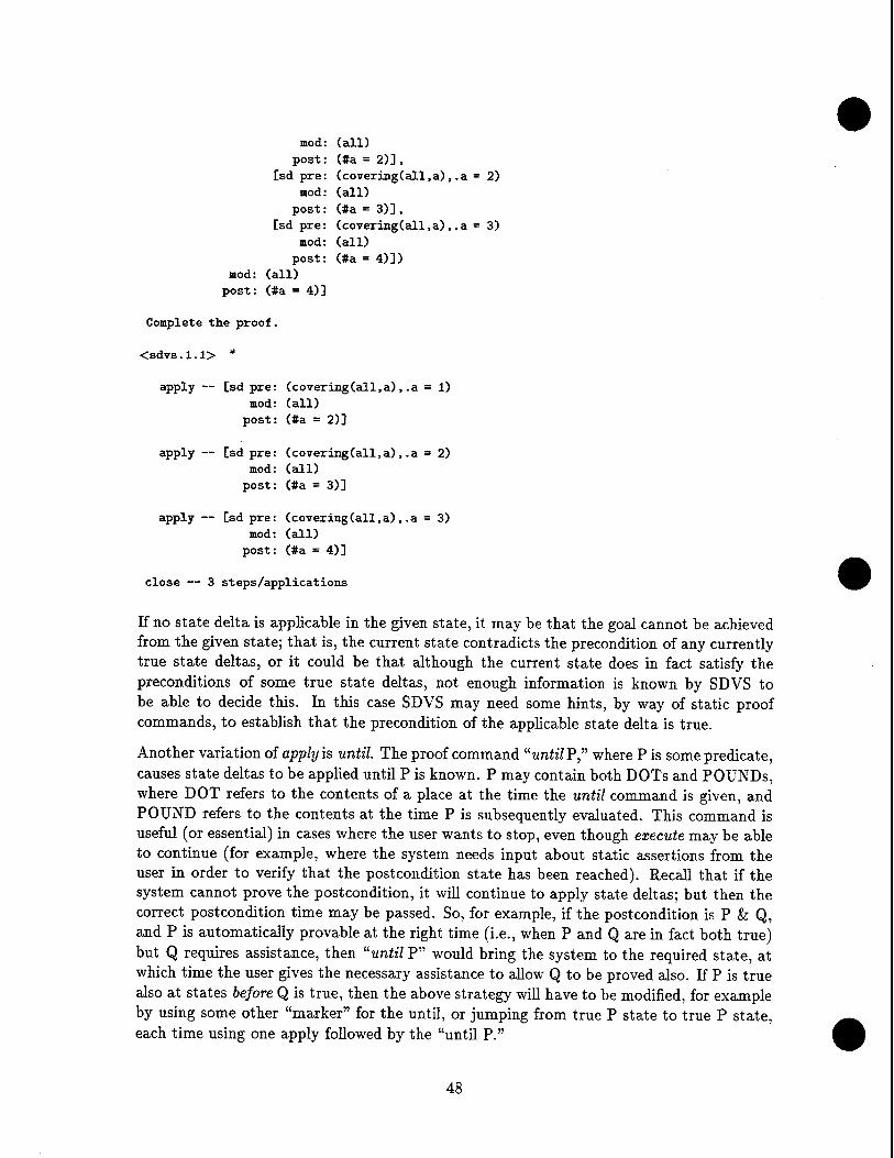
mod: (all) post: (#a = 2)],
[sd pre: (covering(all,a),.a = 2) mod: (all)
post: (#a = 3)], [sd pre: (covering(all,a),.a = 3)
mod: (all) post: (#a =4)])
mod: (all) post: (#a =4)]
Complete the proof.
<sdvs.l.l> *
apply — [sd pre: (covering(all,a),.a = 1) mod: (all)
post: (#a = 2)]
apply — [sd pre: (covering(all,a),.a = 2) mod: (all)
post: (#a = 3)]
apply — [sd pre: (covering(all,a),.a = 3) mod: (all)
post: (#a =4)]
close — 3 steps/applications
If no state delta is applicable in the given state, it may be that the goal cannot be achieved from the given state; that is, the current state contradicts the precondition of any currently true state deltas, or it could be that although the current state does in fact satisfy the preconditions of some true state deltas, not enough information is known by SDVS to be able to decide this. In this case SDVS may need some hints, by way of static proof commands, to establish that the precondition of the applicable state delta is true.
Another variation of apply is until. The proof command u until P" where P is some predicate, causes state deltas to be applied until P is known. P may contain both DOTs and POUNDs, where DOT refers to the contents of a place at the time the until command is given, and POUND refers to the contents at the time P is subsequently evaluated. This command is useful (or essential) in cases where the user wants to stop, even though execute may be able to continue (for example, where the system needs input about static assertions from the user in order to verify that the postcondition state has been reached). Recall that if the system cannot prove the postcondition, it will continue to apply state deltas; but then the correct postcondition time may be passed. So, for example, if the postcondition is P & Q, and P is automatically provable at the right time (i.e., when P and Q are in fact both true) but Q requires assistance, then "until P" would bring the system to the required state, at which time the user gives the necessary assistance to allow Q to be proved also. If P is true also at states before Q is true, then the above strategy will have to be modified, for example by using some other "marker" for the until, or jumping from true P state to true P state, each time using one apply followed by the "until P."
48

Another use for until is the case where the state delta the user wants to apply, say SI, has a precondition that the simplifier cannot prove automatically, and thus another (lower) state delta, say S2, whose precondition is provable is applied instead. In this case the user would make the condition P in "■until P" the postcondition of the last proved state delta, and then insert hints to prove the precondition of SI.
2.4 PROOF BY CASES
A typical instance of proof by cases occurs at a branch point of a program. In order to proceed symbolically to the goal, the current state before the branch must be split into two (or into as many branches as there are), and each branch must be pursued separately. When a split into two is desired, the cases command may be used. When a case proof is desired to achieve a goal other than the current goal, the subcases command is used.
The command syntax is
cases <cond> <thenproof> <elseproof>
where <cond> is some predicate such that the assumption of <cond> allows the choice of branch to be determined, <thenproof> is the proof for that branch, and <elseproof> is the proof for the rest of the computation, which assumes that <cond> is not true. If one or both of <thenproof> and <elseproof> are empty, then SDVS will try to close with no proof. If it is not able to close, it will respond with "complete the proof," and then the user may interactively submit proof commands. The predicate <cond> can be first order or a state delta; see the example in Section 2.9.7. Consider the following example:
<sdvs.2> ppsd state delta: casessd
[sd pre: (f ormula(casesl) ,ionmila(cases2)) mod: (a)
post: (#a gt 0)]
<sdvs.2> ppsd state delta: casesl
[sd pre: (.a It 0) mod: (a) post: (#a = 1)]
<sdvs.2> ppsd state delta: casesZ
[sd pre: (.a ge 0) mod: (a) post: (#a = 2)]
<sdvs.2> init proof name D : < CR>
49
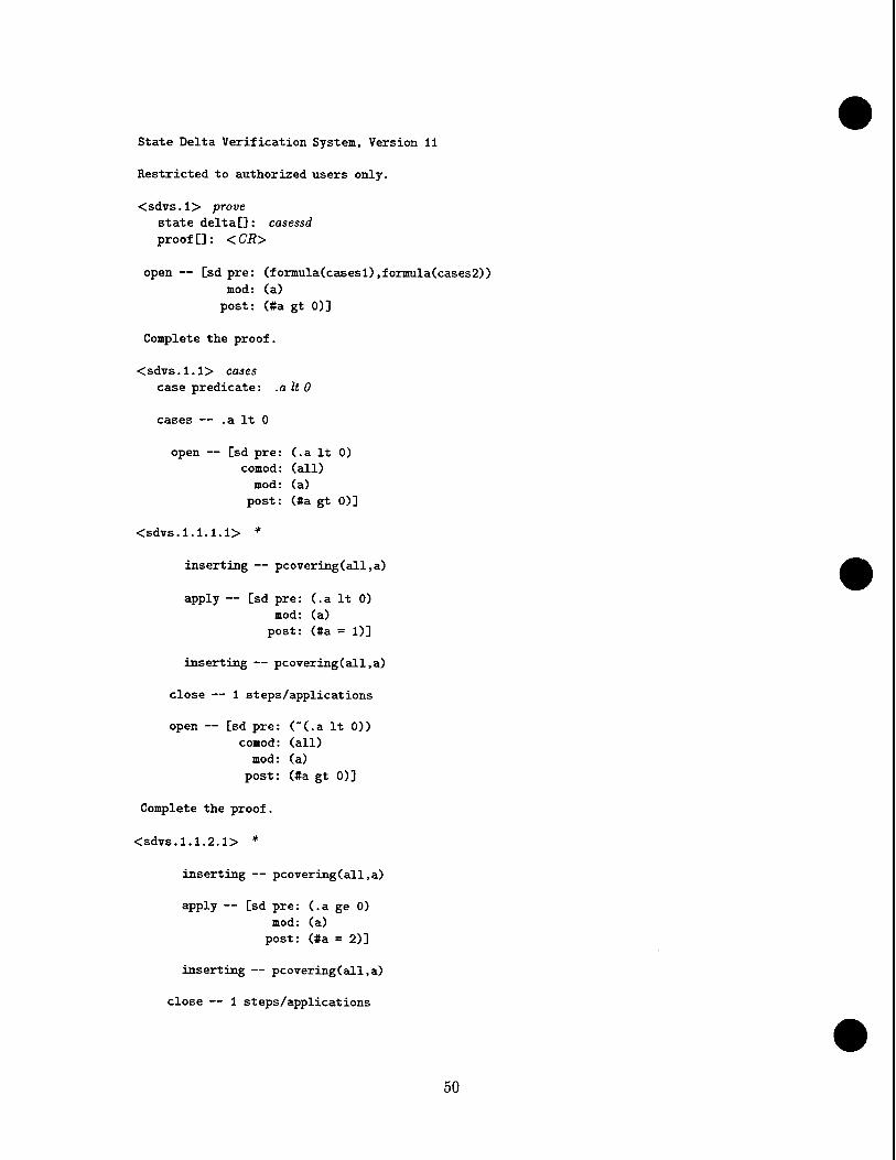
State Delta Verification System, Version 11
Restricted to authorized users only.
<sdvs.l> prove state delta[]: casessd proof []: <CR>
open— [sd pre: (formula(casesl),formula(cases2)) nod: (a)
post: (#a gt 0)]
Complete the proof.
<sdvs.l.l> cases case predicate: .a It 0
cases — .a It 0
open — [sd pre: (.a It 0) comod: (all) mod: (a)
post: (#a gt 0)]
<sdvs.l.l.l.l> *
inserting — pcovering(all.a)
apply — [sd pre: (.a It 0) mod: (a)
post: (#a = 1)]
inserting — pcovering(all,a)
close — 1 steps/applications
open — [sd pre: ("(.a It 0)) comod: (all) mod: (a)
post: (#a gt 0)]
Complete the proof.
<sdvs.l.l.2.1> *
inserting — pcovering(all,a)
apply — [sd pre: (.a ge 0) mod: (a)
post: (#a = 2)]
inserting — pcovering(all,a)
close — 1 steps/applications
50

join — [sd pre: (true) comod: (all) mod: (a)
post: (#a gt 0)]
inserting — pcovering(all.a)
inserting — pcovering(all,a)
close — 1 steps/applications
In this example both cases were proved by the execute command (*). Note that the two subcases were opened, closed, and joined, and the joined state delta was applied to complete the proof of the top level.
When there are more than two cases to consider, and the user wants to describe each explicitly rather than translate the problem into a nested cases, there is the command meases (m for multiple):
meases (<coadl>.<proofl>) (<cond2>.<proof2>) ... (<condn>.<prooin>)
SDVS must be able to prove that the disjunction of the <cond> clauses is true.
For example, consider the following proof:
<sdvs.2> pp object: casesproof
proof casesproof:
prove [sd pre: ([sd pre: (pi 8; p2) mod: (all)
post: (ql)], [sd pre: (pi ft "p2)
mod: (all) post: (q2)],
[sd pre: (~pl ft p2) mod: (all)
post: (q2)], [sd pre: (~pl & "p2)
mod: (all) post: (ql)])
mod: (all) post: (ql or q2)]
proof: meases
(case: pi ft p2 proof: *
51

case: pi ft ~p2 proof: * case: "pi ft p2 proof: * case: "pi ft ~p2 proof: *)
<sdvs.2> init proof name D : casesproof
State Delta Verification System, Version 11
Restricted to authorized users only.
open — [sd pre: ([sd pre: (pi ft p2) mod: (all)
post: (ql)], [sd pre: (pi ft "p2)
mod: (all) post: (q2)],
[sd pre: (~pl ft p2) mod: (all)
post: (q2)], [sd pre: ("pi ft "p2)
mod: (all) post: (ql)])
mod: (all) post: (ql or q2)]
meases — 4
open — [sd pre: (pi ft p2) comod: (all)
mod: (all) post: (ql or q2)]
apply — [sd pre: (pi ft p2) mod: (all)
post: (ql)]
close — 1 steps/applications
open — [sd pre: (pi ft ~p2) comod: (all)
mod: (all) post: (ql or q2)]
apply — [sd pre: (pi ft "p2) mod: (all)
post: (q2)]
close — 1 steps/applications
open — [sd pre: ("pi ft p2) comod: (all)
52

mod: (all) post: (ql or q2)]
apply — [sd pre: ("pi & p2) mod: (all)
post: (q2)]
close — 1 steps/applications
open — [sd pre: (~pl & "p2) comod: (all)
mod: (all) post: (ql or q2)]
apply — [sd pre: (~pl & ~p2) mod: (all)
post: (ql)]
close — 1 steps/applications
join — [sd pre: (pi & p2 or pi & "p2 or ~pl & p2 or ~pl & ~p2)
comod: (all) mod: (all)
post: (ql or q2)]
close — 1 steps/applications
Another variety of cases is subcases. This is used for proving a statement other than the current goal by cases. Of course, there is no essential need for subcases, since starting a new subproof of a state delta with the subcases goal as the postcondition, followed by applying that state delta, will suffice.
The format is
subcases <cond> <mod> <subgoal> <thenproof> <elseproof>.
This is similar to the cases command, but the cases are joined at <subgoal> instead of at the goal of the current proof. The field <mod> is the mod list for each execution path to the subgoal.
<sdvs.l> subcases subcase predicate:
modification list[]: P <CR>
subgoal: then proof D : else proof □ :
p or q <CR> <CR>
subcases — p
53

open — [sd pre: (p) comod: (all) post: (p or q)]
close — 0 steps/applications
open — [sd pre: (~p) comod: (all) post: (p or q)]
Complete the proof.
Of course, the proof is not closed, because the above state delta is not valid.
2.5 PROOF BY INDUCTION
Induction arguments are in general more complex than straight-line symbolic execution or branching. Several useful forms of induction that are applicable in many naturally occurring proofs are identified and incorporated into SDVS 11. SDVS 11 is able to prove claims about terminating loops by induction on the natural numbers using the induct command. A fixed- point induction command for proving claims about TR-generated continuations has been implemented on an experimental basis, but does not appear in robust form in SDVS 11. In addition, there are experimental commands for general mathematical induction (natinduct: see Section 2.9.8) and for proving properties of Ada recursive procedures (recurse) [37]. The omegainduct command (Section 8.5) is primarily intended for proving safety properties of Ada programs.
The induct command allows for proofs of theorems about programs containing certain kinds of loops. Note: the restrictions on the kind of loops make the current implementation unable to handle some cases. However, probably any proof involving induction over a set essentially ordered like the natural numbers is verifiable in this implementation.
Sometimes a proof by induct is a short version of another proof by symbolic execution, if the loop is of known length. For loops with data-dependent length, induction may be the only way to take the proof over the loop.
The typical use of the induct command is when you are at a place in the proof where you want to prove the following state delta (call it Si):
[SD pre: (TRUE) comod: (ALL)
mod: (M) post: (Q)]
and then apply it, bringing the symbolic computation to a state in the future at which Q is true, and during which interval only the places in M have changed.
Proving Si by induction involves finding a predicate Inv(.X) (the invariant) that depends on some number-valued place X such that Inv(n) implies Q for some n, and such that:
54
Inv(O) is true now, i.e.
(1) [SD pre: (TRUE) comod: (ALL)
mod: 0 post: (Inv(O))]
and
(2)[SD pre: (Inv(i)) comod: ()
mod: (M) post: (Inv(i+1))]
If these two state deltas are true, then it is true that for all n,
[SD pre: (TRUE) comod: (ALL)
mod: (M) post: (Inv(n))]
Thus, we can apply this state delta, obtaining Inv(n), and thus Q.
[Note for the advanced SDVS user: the above conclusion is valid if we use any comod list C instead of the empty comod list in (2), as long as C and M are disjoint. However, we strongly suggest (and this may be enforced in later versions of SDVS) that the induct comod list always be chosen to be empty. Similarly we suggest that there be no dots in the induct mod list, for example a[.i] where a is an array place. Instead, use a in the mod list and make the invariant strong enough to imply that part of the array is held constant in the transition represented by the step-case state delta.
However, when using induction to characterize iterations of a loop involving arrays, more care on the user's part might be needed. For example, if one iteration of the loop changes only the slice a[.i: 10], where A has a different value depending on which iteration you are doing, you really would need to give a[.i : 10] as the induct command modlist. Then the state delta representing the net result of all the iterations (the "join state delta" constructed at the successful completion of the induct command) will have simply a in its modlist: there is no simple way to restrict the part of a that may have changed. If in fact a is actually of length 20, say, and you need to preserve the values of a[ll : 20] over the course of the induction, do a
<sdvs.l> let new variable: aa
value: a[l:10]
55

and give aa[.i : 10] as the induct modlist. Then the step-case state delta will preserve the first part of aa, and thus of a, and the join-case state delta will have only aa as its modlist, so that a[ll: 20] will be preserved. End of Note for the advanced SDVS user.]
Actually, SDVS makes the user choose initial ("from") and final ("to") values for .X, instead of using 0 and some arbitrary n. Also, Inv must be a predicate without top-level pounds. It may, and often does, contain state deltas. Inv(./#) is the result of substituting pounds for dots in Inv.
Therefore, SDVS sets up proofs of
(1) [SD pre: (TRUE) comod: (ALL)
mod: () post: (Inv(from))]
and
(2) [SD pre: (Inv(i), i ge from, i It to) comod: (C)
mod: (M) post: (Inv(i+1)(./#))]
If the system can prove these two, then it creates and automatically applies the state delta:
[SD pre: (TRUE) comod: (ALL)
mod: (M) post: (Inv(to)(./#))]
If Inv was chosen shrewdly (for example, if Inv(to) implies Q), then Q will be true in the resulting new state, thus essentially proving and applying Si.
The induct command has eight parameters,
induct <indexp> <from> <to> <invariant> <comod> <mod> <baseproof> <stepproof>
and means "Do an induction proof (of the current goal) using the expression <indexp> in the range <from> to <to>" (both of type integer, with one provably less than or equal to the other); <indexp> can be any expression of type integer that contains only one variable of type place and no pounds. A new (previously undeclared) place may be introduced as
56

the only place in <indexp>. <invariant> (a list of predicates) is the loop invariant. The invariant can also contain state deltas, but cannot contain pounds at the top level. Do not leave the invariant field blank; if you really do not need an invariant, type "true." <comod> and <mod> are the lists for the induction step; they must be disjoint.
In the above typical case, <indexp> is .X, <from> is Initial, <to> is Final, <invariant> is Inv, <comod> is C, <mod> is M, and <baseproof> and <stepproof> would be proofs of the two claims (1) and (2) above. If either <baseproof> or <stepproof> are empty, SDVS tries to close the current proof automatically. If it cannot, it responds with "complete the proof", and then the user may submit interactive proof commands.
The step modification list gives the places that change in executing the loop once, and the step comodification list gives those places that must be preserved for the loop to execute again. These lists must be disjoint. Indeed, the comodification list of the induct command may always be taken to be empty, if the invariant is chosen to be strong enough. Also, the mod list of the induct command must be contained in the mod list of the state delta being proved. However, there need not be any connection between the comodification lists of the two state deltas.
Here is a typical proof. Note that the comodification list is empty, as is the base proof; under certain circumstances related to the pretty-printer, these fields may not show up in the prettyprinted form.
(prove [sd pre: (.a = l,.b = l,covering(all,a,b), [sd pre: (.a = l,.b ge l,covering(all,a,b))
mod: (b) post: (#b = .b + 1)])
mod: (b) post: (#b = 100,#a ge 0)]
proof: induct on: .b
from: 1 to: 100 invariants: (.a= 1) comodlist: modlist: (b) base proof: step proof: apply [sd pre: (.a = l,.b ge 1,covering(all,a,b))
mod: (b) post: (#b = .b + 1)])
And here is a transcript of the proof:
<sdvs. 1.2. 1> init proof name []: pr.eg28proof
State Delta Verification System, Version 11
57

Restricted to authorized users only.
open — [sd pre: (.a = l,.b = 1,covering(all,a,b), [sd pre: (.a = l,.b ge l,covering(all,a,b))
mod: (b) post: (#b = .b + 1)])
mod: (b) post: (#b = 100,#a ge 0)]
induction — .b from 1 to 100
open — [sd pre: (true) comod: (all) post: (.a = 1,.b = 1)]
close — 0 steps/applications
open — [sd pre: (.b ge l,.b It 100,.a = 1) mod: (b)
post: (#a = l,#b = .b + 1)]
apply — [sd pre: (.a = l,.b ge l,covering(all,a,b)) mod: (b)
post: (#b = .b + 1)]
close — 1 steps/applications
join induction cases — [sd pre: (1 le 100) comod: (all)
mod: (b) post: (#b = 100,#a = 1)]
close — 1 steps/applications
If the invariant is left out, then the proof will not go through. However, if the comodification list is made to contain a, the proof will go through with trivial invariant.
A minor change in the state delta will allow both the comodification list and the invariant to be "true:"
[sd pre: (.a = l,.b = l,covering(all,a,b), [sd pre: (.b ge 1,covering(all,a,b))
mod: (b) post: (#b = .b + 1)])
mod: (b) post: (#b = 100,#a ge 0)]
Another option is to use a new name as an induction variable, for example counter. This variable is automatically incremented by 1 every time around the loop, i.e., from the precon- dition to the postcondition of the step-case state delta. See Section 2.1 for another example involving counter.
58

If the induction argument is over a larger well-ordered set, then a more complicated proof will have to be used. For example, we could be faced with the situation of a loop within a loop, where the inner loop bounds are possibly different each time.
For an abstract illustration, consider the pairs of natural numbers ordered lexicographically (the order is u;2). If a loop takes a pair into a lower pair, then there is no finite bound on the number of times around the loop, even in terms of the initial pair. However, the loop does terminate with the value (0,0). Thus, the following state delta ind.sd is true and provable
in SDVS:
[sd pre: (covering(all,a,b),.a ge 0,.b ge 0, [sd pre: (.a gt 0,.b gt 0)
mod: (a,b) post: (#a It .a or #a = .a & #b It .b,#a ge 0,#b ge 0)],
[sd pre: (.a = 0,.b gt 0) mod: (a,b)
post: (#a = .a,#b It .b,#b ge 0)], [sd pre: (.a gt 0,.b = 0)
mod: (a,b) post: (#a It .a,#a ge 0,#b ge 0)])
mod: (a,b) post: (#a = 0,#b = 0)]
Here is the proof 5:
(prove ind.sd proof:
(prove si proof:
(prove si.1 proof:
(let aa = .a, let bb = .b, induct on: k
from: 0 to: bb invariants: (.a It aa or
.a = aa & .b le bb - k, .a ge 0,.b ge 0)
comodlist: modlist: (a,b) base proof: step proof:
cases .b = 0 then proof: else proof:
cases .a gt 0 then proof: apply il else proof: ),
let aa = .a,
5 The proof is due to John Don er.
59

apply sl.l, cases .a = aa then proof: apply i3 else proof: ),
prove s2 proof:
(let aa = .a, induct on: i
from: 0 to: aa invariants: (.a le aa - i,.a ge 0,.b ge 0) comodlist: modiist: (a,b) base proof: step proof:
cases .a = 0 then proof: else proof: apply si),
prove s3 proof:
(let bb = .b, induct on: j
from: 0 to: bb invariants: (.b le bb - j,.a = 0,.b ge 0) comodlist: modiist: (a,b) base proof: step proof:
cases .b = 0 then proof: else proof: apply i2),
cases .a = 0 then proof: apply s3 else proof:
(apply s2, apply s3)))
where si is
[sd pre: (.a gt 0,.b ge 0) mod: (a,b)
post: (#a It .a,#a ge 0,#b ge 0)]
sl.l is
[sd pre: (.a gt 0,.b ge 0) mod: (a,b)
post: (#a It .a or #a = .a ft #b = 0,#a ge 0,#b ge 0)]
s2 is
60

[sd pre: (.a gt 0,.b ge 0) mod: (a,b)
post: (#a = 0,#b ge 0)]
and s3 is
[sd pre: (.a = 0,.b ge 0) mod: (a,b)
post: (#a = 0,#b = 0)]
2.6 PROOF BY CONTRADICTION
In SDVS, if the symbolic execution proof brings about an inconsistent state (e.g., one containing 0 = 1 or x ^ x), then the most recently begun proof is closed, and that state delta that was being proved is proclaimed usable. The explanation is that in opening the proof of that state delta, we assumed that there was a state (subject to the comod list restrictions) that satisfied its precondition, and on the basis of that state we were able to execute forward. If we arrive at an inconsistent state, that must mean that our previous assumption was false. Thus, there was in fact no state satisfying those conditions, and thus the state delta is "vacuously" true.
When trying to achieve the postcondition of the goal state delta, a usable state delta can (only) be applied if its mod list is contained in that of the goal, since that is part of the satisfaction condition. However, if reaching a contradiction is the intended proof strategy, one need not worry about this restriction; in that case we are not executing to the state fulfilling the postcondition, but are simply trying to get to a state manifesting the contradiction in the precondition.
Another way to put this is that if the mod list of an applied state delta is not contained in the mod list of the state delta to be proven, then the only way the proof can be closed is by reaching a contradiction. The user is suitably warned by an SDVS message.
First, we show how proof by contradiction can be exploited to eliminate false cases. The state delta eqdotx below essentially says that if we can execute to a state, allowing x to change along the way, in which we learn that the original value of x was 1, then in fact, the current value of a; is 1. Note that we cannot prove this fact by simply executing to a future state, because the mod list x of the applied state delta is not included in the mod list of the state delta to be proven, which is empty, and thus we would have to reach a contradiction in order to close the proof. But since .x is 1, there is no contradiction. The way to reach a contradiction is first to assume that the current value of x is not 1. This calls for a proof by cases.
<sdvs.l> pp object: dotx
[sd pre: (true) mod: (x) post: (.x = 1)]
61

<sdvs.l> pp object: eqdotx
[sd pre: (formula(dotx)) comod: (all) post: (.x = 1)]
<sdvs.l> prove state deltaD: eqdotx proof [] : < CR>
open — [sd pre: (formula(dotx)) comod: (all) post: (.x = 1)]
Complete the proof.
<sdvs. 1. 1> cases case predicate: .x = 1
cases — .x = 1
open — [sd pre: (.x = 1) comod: (all) post: (x\H6 = 1)]
close — 0 steps/applications
open — [sd pre: (~(.x = 1)) comod: (all) post: (x\116 = 1)]
Complete the proof.
<sdvs.l.l.2.1> usable
u(l) [sd pre: (.x = 1) comod: (all) post: (x\116 = 1)]
u(2) [sd pre: (true) mod: (x) post: (.x = 1)]
No usable quantified formulas.
<sdvs.l.l.2.1> apply sd/number[highest applicable/once]: <CR>
inserting — pcovering(all.x)
apply — [sd pre: (true) mod: (x)
post: (.x = 1)]
Warning: the modlist of the last applied state delta mentions places
62

(x) outside of the modlist of the state delta to be proven. The
current proof can only be closed by contradiction.
The postcondition of the last applied state delta is inconsistent
with the current state.
close — 0 steps/applications
join — [sd pre: (true)
comod: (all)
post: (x\116 = 1)]
close — 1 steps/applications
Now here is the example from Section 1.5. This shows how we may sometimes want to execute to achieve a false state in order to prove the inconsistency of a precondition.
<sdvs.l> ppsd state delta: covsd
[sd pre: (covering(a,c,d)) mod: (d)
post: (#c = .c + 1)]
<sdvs.l> ppsd state delta: contrasd
[sd pre: (formula(covsd),covering(a,c,d)) mod: (all)
post: (false)]
<sdvs.l> prove state delta[] : contrasd proof [] : < CR>
open— [sd pre: (formula(covsd),covering(a,c,d)) mod: (all)
post: (false)]
Complete the proof.
<sdvs. 1. 1> usablesds
u(l) [sd pre: (covering(a,c,d)) mod: (d)
post: (#c = .c + 1)]
<sdvs.l.l> apply sd/number[highest applicable/once]: <CR>
apply — [sd pre: (covering(a,c,d)) mod: (d)
post: (#c = .c + 1)]
63

The postcondition of the last applied state delta is inconsistent with the current state.
close — 0 steps/applications
The final example shows how to prove that if p can bring about false, then p holds in the current state.
<sdvs.l> prove state delta[] : negateS.sd proof []: <CR>
open — [sd pre: ([sd pre: (p) comod: (all)
mod: (all) post: (false)])
post: ("p)]
Complete the proof.
<sdvs.l.l> cases case predicate: p
cases — p
open — [sd pre: (p) comod: (all) post: (~p)]
<sdvs.l.l.l.l> usable
u(l) [sd pre: (p) comod: (all) mod: (all) post: (false)]
No usable quantified formulas.
Now we would like to apply u(l) to bring about false and thereby negate the precondition.
<sdvs.l.l.l.l> apply sd/number[highest applicable/once]: u
number: 1
apply — [sd pre: (p) comod: (all)
mod: (all) post: (false)]
Warning: the modlist of the last applied state delta mentions places (all) outside of the modlist of the state delta to be proven. The current proof can only be closed by contradiction.
64

The postcondition of the last applied state delta is inconsistent with the current state.
close — 0 steps/applications
open — [sd pre: ("p) comod: (all) post: (~p)]
close — 0 steps/applications
join — [sd pre: (true) comod: (all) post: (~p)]
close — 1 steps/applications
2.7 STATIC PROOF
Now we describe the static proof language. These commands relate only to deductions within a given state. They do not open or apply state deltas, though they certainly can cause state deltas to close.
There are essentially three different ways in which the system can prove static assertions, i.e., that a static assertion A follows from the database D:
1. Automatically: The assertion follows from the database without any user interaction; the system "knows" it to be true.
2. Proof by "axiom" or "lemma" invocation: The assertion A follows by axiom or lemma invocation from database D if there is an axiom or lemma of the form "if C then P," where A is of the pattern P and C follows from D automatically. This is implemented so that the user need not, but may, specify the axiom or lemma to be used to verify A. If no name is specified, SDVS checks all the axioms or lemmas with the required pattern until it finds one with the provable precondition C. (Note that the appropriate list of axioms must be read before being used. The command help axioms gives the names of the files of axioms.) The database is then updated by adding A. The choice of the word "axiom" simply indicates that these rules are useful and basic enough to be built into SDVS. Of course, they are not independent or necessarily elegant. "Lemmas" are rules that the user may create and prove from the axioms and already proven lemmas.
3. Proof "by notice": In the case that A does not follow automatically from the database D or by axiom or lemma, one must construct a sequence A\,..., An such that A\ follows automatically from D, A{ follows automatically from D, Ai,..., A,-_i, and A is An. This is implemented by the notice command. Thus, notice Ai checks to see whether A{ follows (automatically) from the current database, and if so, updates the database by adding A; explicitly.
Chapter 9, on the simplifier, specifies how much about a given domain is fully automated knowledge (decision procedures) and how much is partially automated.
65

2.7.1 Axioms
The provebyaxiom command causes the system to try to prove the subsequent statement by invoking an axiom. An axiom is represented as a pattern of the form (implies q p), or just p [equivalent to (implies true p)], where q and p are predicate patterns that may contain free variables. A single instantiation of an axiom can be used to prove the truth of a formula that "matches" the consequent of the axiom "at the top level." By "matches at the top level" we mean that the axiom consequent (p) has the same syntactic form as the formula, except for free variables, which match arbitrary terms. If a free variable is duplicated, then the formula must have identical terms that match the multiple occurrences of the free variable.
Consider a formula F and an axiom A of the form (implies q p). We say that "A proves F" if and only if p matches F at the top level, and q, when instantiated, simplifies (in SDVS) to TRUE. An axiom pattern is instantiated by the replacement of all of its free variables with matched terms taken from the formula. In mathematical notation, if p and q are of the form p(xx,... ,x„) and q(xi, ...,xn) then F has to be of the form p{tu. ..,<„) for terms U, and q(ti,. ..,tn) must simplify to TRUE.
The syntax of the command is provebyaxiom <expr> <axiom-name>. If <axiom-name> is omitted, the system will search the list of all currently loaded axioms to try to find one with the right pattern. The system prompts for instantiations of variables that appear on the left side but not on the right side.
This next little example only illustrates what would happen if test.ax really were an axiom. You cannot duplicate this without using the createaxiom command, which we like to dis- courage.
<sdvs.l> pp object: axiom axiom name: test.ax
axiom test.ax (x.y.z): p(x,y) —> q(x,z)
<sdvs.l> prove state delta[]: test.sd proof []: <CR>
open— [sdpre: (p(l,2)) post: (q(l,3))]
Complete the proof.
<sdvs.l.l> provebyaxiom formula to prove: q(l, 8)
axiom name[] : test.ax match for y: 2
provebyaxiom test.ax — q(l,3)
close — 1 steps/applications
66

The following is a list of the commands related to axioms that are illustrated in the example below:
<sdvs.l> read path name[testproofs/foo.proofs] : axioms/arraycoverings.axioms
Definitions read from file "axioms/arraycoverings.axioms" — (disjoint\adjacent\slices,disjoint\slices,disjoint\elements,
pcovering\slice,pcovering\element,pcovering\slice\slice, pcovering\slice\element,disjoint\slice\element)
<sdvs.2> axiornnames symbol list[]: <CR>
Axiom names — (pcovering\slice\element,pcovering\slice\slice, pcovering\element,pcovering\slice,disjoint\slice\element, disjoint\elements,disjoint\slices, disjoint\adjacent\slices,test.ax)
<sdvs.2> pp object: axioms axiom names[] : <CR> with, symbolsD : <CR>
axiom pcovering\slice\element (a,i,m,n): (disjointarray(a) & m le i) ft i le n —> pcovering(a[m:n] ,a[i])
axiom pcovering\slice\slice (a,i,j,m,n): ((disjointarray(a) ft m le i) ft i le j) j le n —> pcovering(a[m:n],a[i:j])
axiom pcovering\element (a,i): disjointarray(a) —> pcovering(a,a[i])
axiom pcovering\slice (a,i,j): disjointarray(a) —> pcovering(a,a[i:j])
axiom disjoint\slice\element (a,i,m,n): disjointarray(a) ft (m gt i or i gt n) —> alldisjoint(a[m:n] ,a[i])
axiom disjoint\elements (a,i,j): disjointarray(a) ft i "= j —> alldisjoint(a[i3 ,a[j])
axiom disjoint\slices (a,i,j,k,l): disjointarray(a) ft (j It k or 1 It i) —> alldisjoint(a[i:j],a[k:l])
axiom disjoint\adjacent\slices (a,i,j,k,l): ((disjointarray(a) ft j ge i) ft j + 1 = k) ft
1 ge k —> covering(a[i:l],a[i:j], a[k:l])
axiom test.ax (x,y,z): p(x,y) —> q(x,z)
<sdvs.2> pp ob j ect: axioms axiom names [] : < CR>
67

with symbols D : pcovering
axiom pcovering\slice\element (a,i,m,n): (disjointarray(a) ft m le i) ft i le n —> pcovering(a[m:n] ,a[i])
axiom pcovering\slice\slice (a,i,j,m,n): ((disjointarray(a) ft m le i) ft i le j) ft j le n —> pcovering(a[m:n],a[i:j])
axiom pcovering\element (a,i): disjointarray(a) —> pcovering(a,a[i])
axiom pcovering\slice (a.i.j): disjointarray(a) —> pcovering(a,a[i:j])
<sdvs.2> axiomnames symbol list [] : pcovering
Axiom names with symbol pcovering — (pcovering\slice\element, pcovering\slice\slice, pcovering\element,pcovering\slice)
<sdvs.2> pp object: axioms axiom names 0: disjoint\elements
axiom disjoiat\elements (a,i,j): disjointarray(a) ft i "= j —> alldisjoint(a[i] ,a[j])
Now assume that we know that a is a disjoint array. Then SDVS automatically knows (if the array solver is active) that a[i] and a[j] are alldisjoint for any two distinct integers i, j, whether or not they are in range (real indices).
<sdvs.2> simp expression: disjointarray(a) -> alldisjoint(a[l], a[2])
true
Also,
<sdvs.2> simp expression: (disjointarray(a) and i '= j) -> alldisjoint(a[l], a[2j)
true
The axiom disjoint\elements is used in the case that a[i] and a[j] are introduced before the system knows that i ~= j. For example:
<sdvs.3> prove state delta[] : disjoints.sd proof [] : < CR>
68

open— [sd pre: (declare(a,type(array,l,2,type(bitstring,8))), .aCi] = .a[j])
post: (false)]
Complete the proof.
<sdvs. 3. 1> cases case predicate: i = j
cases — i = j
open — [sd pre: (i = j) comod: (all) post: (false)]
<sdvs.3.1.1.1> defer numbers of goals[all]: < CR>
deferring all current goals
close — 1 steps/applications
open — [sd pre: (~(i = j)) comod: (all) post: (false)]
Complete the proof.
<sdvs.3.1.2.1> simp expression: alldisjoint(a[i], a[jj)
alldisjoint(a[i] ,a[j])
<sdvs.3.1.2.1> provebyaxiom formula to prove: alldisjoint(a[i], a[j])
axiom name D: disjoint\elements
provebyaxiom disjoint\elements — alldisjoint(a[i] ,a[j])
<sdvs.3.1.2.2> simp expression: alldisjoint(a[i], a[j])
true
2.7.2 Rewriting
The rewrite command is based on the mechanism for invoking axioms and applies to equality assertions that are provable by existing axioms. When the user wants to cause an equality between two terms to be asserted, but does not want (or need) to write the "simpler" term, he or she may simply type rewritebyaxiom x. The system then scans the axioms to find an equality axiom based on the pattern of x (on either side of the equality) and causes the equality to be asserted. Again, the name of the axiom desired to do the rewriting may be
69

added to the end of the command.
Another method has been implemented for rewriting when not all the variables appear on one side of the equality to be rewritten. However, the general mechanism whereby SDVS prompts for unmatched variables (appearing on the left side of the implication but not the right side), as in the case of provebyaxiom, has not been implemented for rewritebyaxiom. For example, consider the axiom
ussub\ussub (x,h,i,j,k,l,m): h = min(i,k + max(j.O)) ft m = max(j,0) + max(l.O) —> x<i:j><k:l> = x<h:m>
As a matter of convenience, the user may want to say rewritebyaxiom x <i: j><k:n>. This is possible only if the precondition is true. However, since some variables in the precondition do not have matches in the input term, there is nothing to check. In this case, the system will substitute the correct values for h and m.
<sdvs. 1> prove state delta[] : rewrite.sd proof [] : < CR>
open — [sd pre: (h = min(i,k + max(j,0)) ft m = max(j.O) + max(n,0))
post: (x<i:jxk:n> = x<h:m>)]
Complete the proof.
<sdvs. 1. 1> rewritebyaxiom term to rewrite: x<i:j><k:n>
axiom name[]: ussub\ussub
rewritebyaxiom ussub\ussub — x<i:jxk:n> = x<min(i,k + max(j.O))
:max(j,0) + max(n,0)>
close — 1 steps/applications
Note that if the bitstring solver were activated at level 3 or 4, then the above proof would have closed because the simplifier would know the truth of the implication to be proved (remember that solvers must be activated before init):
<sdvs.l> activate solver: bS
Bitstring solver (level 3) activated.
<sdvs.3> prove
70

State delta[]: rewrite.sd proof []: <CR>
open — [sd pre: (h = min(i,k + max(j.O)) & m = max(j,0) + max(n,0))
post: (x<i:j><k:n> = x<h:m>)]
close — 0 steps/applications
2.7.3 Current Axiom List
The axioms axe grouped according to the domain to which they apply. The intent is that each group be complete for its domain; i.e., every (universal) true statement about that domain can be proved from the axioms. In addition, there is a supply of less "basic" axioms that have been found to be useful in actual proofs. For example, in the bitstring domain there are axioms for distributing substring over concatenation, for compressing concatenation, and so on.
The user may peruse the list of axioms of the domain of interest to see if there is an axiom that will exactly solve a given problem, or one may use the command axiomnames or pp < CR> axioms with the symbol or symbols of interest. The "symbol" refers to the actual symbol in the axiom, and not in the name of the axiom. Also note that it is the alphabetic name, not the mathematical symbol, e.g. "mult" not "*". The simplifier names of the symbols used in the axioms can be obtained by the help symbols query:
constants everyplace, emptyplace, emptyarray, true, false
functions mkarray, bitvecwave, val, inertial.update, transport.update, transaction, waveform, abs, mod, rent, div (/), min, max, expt (~), mult (*), minus (-), plus (+), parity, lastone, ones, zeros, useqv, usnor, usnand, usxor, usor, usand (&fe), usnot (""), usremainder (usmod), usquotient (//), ustimes (**), usdifference (--), usplus (++), usgeq (usge), usgtr (usgt), usleq (usle), uslss (uslt), usneq ("==), useql (==), usconc (@), ussub, bcons, bs, usval, lh, aconc, element, origin, range, slice, union, diff, time, timeglobal, timedelta, timeplus, tcval
predicates timege, timegt, timele, timelt, timep, sd-value, It, le, gt, ge, alldisjoint, pcovering, covering, disjointarray, lhp, usvalp, elt, ele, egt, ege, esucc, epred, cond, and (&), or, xor, implies (-->), not ("), eq (=), neq ("=), distinct, bitwaveformp, bitstringwaveformp, preemption
If a particular claim proven by a sequence of steps involving axioms is to be used more than
71

once, it may be advisable to make a lemma by createlemma, which then may be reused.
Below we list all SDVS axioms, grouped by filename. The following list is given as response to the help axioms query:
<sdvs.l> help with [all] : axioms
<«SDVS Help>>> Axioms <<<SDVS Help>»
axioms/abs.axioms integer absolute value
axioms/arraycoverings.axioms arrays and coverings
axioms/arrays.axioms 0-origin arrays (obsolete)
axioms/bitstring.axioms bitstrings
axioms/div.axioms integer division
axioms/exp.axioms integer exponentiation
axioms/idiv.axioms unsigned integer division
axioms/lastone.axioms the LAST.ONE bitstring function
axioms/log2.axioms integer log base 2
axioms/minmax.axioms integer min and max
axioms/mod.axioms integer modulus
axioms/mult.axioms integer multiplication
axioms/origin-arrays.axioms arbitrary-origin arrays
axioms/quant.axioms quantification
axioms/rem.axioms integer remainder
axioms/sqrt.axioms integer square root
Axioms for Integer Absolute value (contained in file axioms/abs.axioms):
abs\pos abs\pos (x) : x ge 0 —> abs (x) = x
abs\neg abs\neg (x) : x It 0 —> abs (x) = -x
Axioms for Bitstrings (contained in file axioms/bitstring.axioms):
72

usval\lt\lh usval\lt\lh (b): 2 ' lh(b) gt |b|
ussub\ltO ussub\ltO (x,i,j): 0 ge j —> x<i:j> = x<i:0>
ussub\usdifierence ussub\usdifference (u,v,x,y,m,n): u = |x| ft (v = |y| &
(u ge v ft (n = 0 ft
2 " (m + 1) gt u - v))) —> |(x — y)<m:n>| = u - v
ussub\ustimes ussub\ustimes (x.y.i.j): j = 0 ft 2 " i gt |x| * |y| —> |(x ** y)<i:j>| = |x ** y|
ussub\ustimes\0 ussub\ustimes\0 (x,y,i,j): 2 " j gt |x| * [y| —> |(x ** y)<i:j>| = 0
usval\ussub\0 usval\ussub\0 (x,i,j): |x| = 0 —> |x<i:j>| = 0
usor\usplus usor\usplus (x,y,z): lb(x) = 1 ft (lh(y) = 1 ft z = 1(1)) --> x usor y = (z ++ (x ++ y))<l:l>
usorO usorO (x,y): |x| = 0 ft lh(y) ge lh(x) —> x usor yj= y
equsvals equsvals (x,y,i,j): W = |y| —> lx<i;j>l = |y<i:J>l
usandl usandl (x,y): x = 1(1) ft lh(y) = 1 —> x ftft y = y
Tissub\usand ussub\usand (x,y,i,j): (x ftft y)<i:j> = x<i:j> ftft y<i:j>
ussub\usxor ussub\usxor (x,y,i,j): (x usxor y)<i:j> = x<i:j> usxor y<i:j>
ussub\usor ussub\usor (x,y,i,j): (x usor y)<i:j> = x<i:j> usor y<i:j>
ussub\usplus\ussub ussub\usplus\ussub (x,y,i, j ,k,l,n,n) : j = 0 ft (1 = 0 ft (i ge m & It ge m)) --> (x<i:j> ++ y<k:l>)<m:a> = (x ++ y)<m:n>
usxorO usxorO (x,y): lh(x) = 1 ft x = y —> x usxor y = 0(1)
usxorl usxorl (x,y): lh(x) = 1 ft (lb.(y) = 1 ft x "= y) —> x usxor y = 1(1)
usorl usorl (x,y): lh(x) = 1 ft (lh(y) = 1 ft (x = 1(1) or y = 1(D)) —> x usor y = 1(1)
usandO usandO (x,y): lh(x) = 1 ft (lb.(y) = 1 ft (x = 0(1) or y = 0(1))) —> x ftft y = 0(1)
restrict\ussub restrict\ussub (x,y,i, j ,k,l,m,n): m ge 0 ft (n ge 0 ft |x<i:j>| = |y<k:l>|) --> |x<i - m:j + n>| = |y<k - m:l + n>|
ussub\ussub ussub\ussub (x,h,i,j,k,l,m): h = min(i,k + max(j,0)) ft m = max(j,0) + max(l,0) —> x<i:j><k:l> = x<h:m>
usval\usconc usval\usconc (x,y,l): 1 = lh(y) —> |x Q y| = |x| * 2 * 1 + |y|
chop chop (x,y,l): lh(x) ge lh(y) ft
73

(2 * lh(x) - 1 ge |x| + |y| ft 1 = lh(x) - 1) —> |x ++ y| = |(x ++ y)<l:0>|
usval\ussub2 usval\ussub2 (x,y,i,j): i = lh(x) - 1 ft (j = 0 ft |x| = |y|) —> |x| = |y<i:j>|
usval\ussub usval\ussub (x,i,j): |x<i:j>| = idiv(irem(|x|,
2 * (min(i,lh(x) - 1) + 1)), 2 " max(j.O))
squash squash (x,i,j,k,l): j = k + 1 ft ((1 ge 1 or 0 ge 1) ft
(i ge j or i ge lh(x) - 1)) —> x<i:j> Q x<k:l> = x<i:l>
ussub\usconc ussub\usconc (x,y,i, j ,il, jl): il = i - lh(y) ft jl = j - lh(y) —> (x « y)<i:j> = x<il:jl> 8 y<i:j>
usval\usconc\0 usval\usconc\0 (x,y): |x] = 0 —> |x 6 y| = [y|
ussub\usplus ussub\usplus (x,y,m,n,u,v) : 2 * n gt |x<n - 1:0> ++ y<n - 1:0>| ft (2 ~ (m + 1) gt |x<m:0> ++ y<m:0>| ft
(u = |x<m:n>| ft v = |y<m:n>|)) —> |(x ++ y)<m:n>| = u + v
chop\general chop\general (x,i,j): j = 0 ft 2 " (i + 1) gt |x| —> |x<i:j>| = |x|
usxor\usplus usxor\usplus (x,y): lh(x) = 1 ft lh(y) = 1 —> x usxor y = (x ++ y) <0:0>
usand\usplus usand\usplus (x,y): lh(x) = 1 ft lh(y) = 1 —> x ftft y = (x ++ y)<l:l>
notO notO (x) : lh(x) = 1 ft x ~= 0(1) ~> x = 1(1)
notl notl (x): lh(x) = 1 ft x "= 1(1) —> x = 0(1)
usor\commute usor\commute (x,y): x usor y = y usor x
commuteusand commuteusand (x,y): x ftft y = y ftft x
lh\ussub lh\ussub (b,i,j): lh(b<i:j>) = max(0,
1 + (min(lh(b) - l,i) - max(0,j)))
lh\ones lh\ones (n): lh(ones(n)) = max(n,0)
lh\zeros lh\zeros (n): lh(zeros(n)) = max(n,0)
lh\usdifference lh\usdifference (ll,12,x,y): 11 = lh(x) ft 12 = lh(y) —> lh(x — y) -^ max(ll,12) + 1
usval\usdifierence\2 usval\usdifference\2 (u,v,x,y,l): u = |x| ft (v = |y| ft
(v gt u ft 1 = max(lh(x),lh(y)) + 1))
—> |x -- y| = 2 " 1 + (u - v)
74

usval\usdiiference\l usval\usdifference\l (x,y,u,v): u = |x| & (v = |y| 4 u ge v) —> |x — y| = u - v
ussub\total ussub\total (j,k,b): j ge lh(b) - 1 & 0 ge k —> b = b<j:k>
ussub\gt\lh ussub\gt\lh (j,k,b): j ge lh(b) - 1 --> b<j:k> = b<lh(b) - l:k>
ussub\empty ussub\empty (x,i,j): i It j —> x<i:j> = 0(0)
usval\ge\0 usval\ge\0 (b): |b| ge 0
usval\le usval\le (x,i,j,k,l): i ge k & 1 ge j —> |x<i:j>| ge |x<k:l>|
ge\usval\usor ge\usval\usor (bl,b2): |bl usor b2| ge |bl|
Axioms for Integer Multiplication (contained in file axioms/mult.axioms):
multgt multgt (x,y,z): x gt 0 ft y gt z or 0 gt x & z gt y —> x * y gt x * z
multltO multltO (x,y): 0 gt x & y gt 0 or x gt 0 & 0 gt y —> 0 gt x * y
multgtO multgtO (x,y): Ogtx&OgtyorxgtO&ygtO —> x * y gt 0
multge multge (x,y,z): x ge 0 & y ge z or 0 ge x & z ge y —> x * y ge x * z
multleO multleO (x,y): 0 ge x ft y ge 0 or x ge 0 & 0 ge y —> 0 ge x * y
multgeO multgeO (x,y): 0 ge x ft 0 ge y or x ge 0 ft y ge 0 —> x * y ge 0
multsquaregeO multsquaregeO (x): x * x ge 0
multmimis multminus (x,y): (-x) * y = -(x * y)
multdistributeminus multdistributeminus (x,y,z): x*(y-z)=x*y-x*z
multdistributeplus multdistributeplus (x,y,z): x*(y+z)=x*y+x*z
multassoc multassoc (x,y,z): x * (y * z) = (x * y) * z
multcommute multcommute (x,y): x*y=y*x
multl multl (x,y): y = 1 —> x * y = x
multO multO (x,y): y = 0 —> x * y = 0
Axioms for Integer Exponentiation (contained in file axioms/exp.axioms):
multeqsquare multeqsquare (a): a * a = a " 2
75

expdiv expdiv (a,k): k ge 1 —> a-(k-l)=a*k/a
expmult expmult (a,k): k ge 1 —> a"k=a*a" (k-1)
e5 e5 (x,a) : a = 0 ft x "= 0 —> a " x = 0
e4 e4 (a,x): a = 0 ft x "= 0 —> x " a = 1
e3 e3 (a,b,c,x): c = a + b --> x"a*x"b = x"c
expabsval expabsval (a,b,c): ((b ge a ft a ge -b) ft b ge 0) ft c ge 1 —> b " c ge a " c
ell ell (a,b,c): (c gt 0 ft b ge 0) ft a ge b —> a * c ge b * c
e8 e8 (a,x,y): (a ge 1 ft x ge 1) ft x ge y —> x * a ge y
e2 e2 (b,x,y): b ge 0 ft y ge x —> b " y ge b * x
elO elO (a.b.c): (c gt 0 ft b ge 0) ft a gt b —> a * c gt b * c
e9 e9 (a,x,y): (a ge 2 ft x ge 2) ft x ge y —> x " a gt y
e7 e7 (b,x,y): b gt 1 ft y gt x —> b " y gt b * x
e6 e6 (a,x): a gt 1 ft 0 gt x —> 1 gt a " x
el el (b,x): b gt 0 ft x ge 0 —> b " x gt 0
Axioms for Min-Max Functions (contained in file axioms/minmax.axioms):
maxge maxge (x,y): max(x.y) ge x
minie minle (x,y): x ge min(x.y)
lemin lemin (x,y,z): y ge x ft z ge x —> min(y.z) ge x
gemax gemax (x,y,z): x ge y ft x ge z —> x ge max(y.z)
gemin gemin (x.y.z): x ge y or x ge z —> x ge min(y.z)
lemax lemax (x.y.z): y ge x or z ge x —> max(j,z) ge x
mineq miaeq (x,y): min(x,y) "= x —> min(x,y) = y
maxeq maxeq (x,y): max(x.y) ~= x —> max(x.y) = y
commutemax commutemax (x,y): max(x,y) = max(y,x)
comautemiii conunutemin (x,y): min(x,y) = mixi(y,x)
Axioms for Coverings of Arrays (contained in file axioms/arraycoverings.axioms):
76

pcovering\slice\element pcovering\slice\element (a,i,m,n): (disjointarray(a) ft m le i) ft i le n —> pcovering(a[m:n] ,a[i])
pcovering\slice\slice pcovering\slice\slice (a,i,j,m,n): ((disjointarray(a) ft m le i) ft i le j) j le n —> pcovering(a[m:n],a[i:j])
pcovering\element pcovering\element (a,i): disjointarray(a) —> pcovering(a,a[i])
pcovering\slice pcovering\slice (a,i,j): disjointarray(a) —> pcovering(a,ati:j])
disjoint\slice\element disjoint\slice\element (a,i,m,n): disjointarray(a) ft (m gt i or i gt n) —> alldisjoint(a[m:n],a[i])
disjoint\elements disjoint\elements (a,i,j): disjointarray(a) ft i "= j —> alldisjoint(a[i], aCj])
disjoint\slices disjoint\slices (a,i,j,k,l): disjointarray(a) ft (j It k or 1 It i) —> alldisjoiat(a[i: j] ,a[k:l])
disjoint\adjacent\slices disjoint\adjacent\slices (a,i,j,k,l): ((disjointarray(a) ft j ge i) ft j + 1 = k) ft
1 ge k —> covering(a[i:l],a[i:j] ,a[k:l])
Axioms for Arrays with Arbitrary Origin (contained in file axioms/origin-arrays.axioms)
emptyslice emptyslice (v,i,j): i gt j —> v[i:j] = emptyarray
lowerslice lowerslice (v,i,j,lb): lb = origin(v) ft origin(v) gt i —> v[i:j] = v[lb:j]
upperslice upperslice (v,i,j,ub): ub = (origin(v) + range(v)) - 1 ft j ge ub —> v[i:j] = v[i:ub]
totalslice totalslice (v,i,j): origin(v) ge i ft j ge (origin(v) + range(v)) - 1 —> v[i:j] = v
siicerange slicerange (v,i,j,r): ((i ge origin(v) ft j ge i) ft origin(v) + range(y) gt j) ft
r = (j - i) + 1 —> range(v[i:j]) = r
sliceorigin sliceorigin (v,i,j): (i ge origin(v) ft j ge i) ft origin(v) + range(v) gt j —> origin(v[i:j]) = i
adjacentslices adjacentslices (v,i,j,k,l): (j ge i ft j = k + 1) ft 1 ge k —> aconc(v[i:j] ,v[k:l]) = v[i:l]
elementofslice elementofslice (v,i,j,k,m): (j ge i ft i ge origin(v)) ft m = (i + k) - origin(v) —> v[i:j][k] = v[m]
elementofaconcl elementofaconcl (vl,v2,j): origin(vl) + range(vl) gt j —> aconc(vl,v2)[j] = vl[j]
elementofaconc2 elementofaconc2 (vl,v2,j,k): j ge origin(vl) + range(vl) ft k = origin(v2) +
(j - (origin(vl) + range(vl)))

—> aconc(vl,v2)[j] = v2[k]
sliceofaconc sliceofaconc (vl,v2,i,j,i2,j2): i2 = origia(v2) + (i - (origin(vl) + range(vl))) &
j2 = origin(v2) + (j - (origin(vl) + range(vl)))
—> aconc(vl,v2)[i:j] = aconc(vl[i: j] ,v2[i2: j2])
Axioms for Log Base 2 (contained in file axioms/]og2.axioms):
log2expgt log2expgt (x,y): x ge 1 ft y = log2(x) —> 2 * (y + 1) gt x
log2exple log2exple (x,y): x ge 1 ft y = log2(x) —> 2 " y le x
log2def log2def (x,y): (x ge 1 ft 2 ' y le x) ft 2 " (y + 1) gt x —> y = log2(x)
Axioms for Integer Division (contained in file axioms/div.axioms):
divgtO divgtO (a,b): (a ge 0 ft b gt 0) ft a ge b or (0 ge a ft 0 gt b) ft b ge a —> a / b gt 0
divltO divltO (a,b): (a ge 0 ft 0 gt b) ft b gt a or (0 ge a ft b gt 0) ft a gt b —> 0 gt a / b
divlt divlt (a,b): a gt 0 & b gt 1 —> a gt a / b
diveqO diveqO (a,b): (a = 0 ft b ~= 0 or a ge 0 fe b gt a) or 0 ge a ft a gt b —> a / b = 0
diveql diveql (a,b) : a = b ft b "= 0 —> a / b = 1
divnegl divnegl (a,b): (-a) / b = -(a / b)
divneg2 divneg2 (a,b): a / (-b) = -(a / b)
divmulteq divmulteq (a,b): a ge 1 —> (a * b) / a = b
divdistl divdistl (a,b,n): ((n gt 0 ft a ge 0) ft b It n) ft 0 le b —> (n*a + b) /n=a
divby2repeat divby2repeat (a,j): j ge 0
—> (a / 2 " j) / 2 = a / 2 " (j + 1)
divgeO divgeO (a,b) : a ge 0 ft b gt 0 or 0 ge a ft 0 gt b —> a / b ge 0
divleO divleO (a,b): a ge 0 ft 0 gt b or 0 ge a ft b gt 0 —> 0 ge a / b
divgemult divgemult (a,b) : a ge 0 ft b '= 0 — > a ge (a / b) * b
divlemult divlemult (a,b): 0 ge a ft b "= 0 —> (a / b) * b ge a
divposlemax divposlemax (a,b): a ge 0 ft b gt 0
78

—> (a / b) * b ge max(0,(a - b) + 1)
divposorder divposorder (a,b,c): a ge 1 & c ge b —> c / a ge b / a
Axioms for Modulo Arithmetic (contained in file axioms/mod.axioms):
modpos modpos (x,y): y gt 0 —> x mod y ge 0
modneg modneg (x,y): 0 gt y —> 0 ge x mod y
modO modO (x,y): x = 0 —> x mod y = 0
modmult modmult (x,y,k): x mod y = Cx + k * y) mod y
modreml modreml (x,y): (y ~= 0 ft (x / y) * y = x or 0 gt x & 0 gt y) or x gt 0 & y gt 0 —> x mod y = x rem y
modrem2 modrem2 (x,y): (y ~= 0 ft (x / y) * y ~= x) & (0 gt x ft y gt 0 or x gt 0 ft 0 gt y) —> abs(x rem y) = abs(y) - abs(x mod y)
Axioms for Remainder Function (contained in file axioms/rem.axioms):
remdef remdef (x,y): y "= 0 —> x=(x/y)*y + x rem y
remO remO (x,y): x = 0 —> x rem y = 0
rempos rempos (x,y): x gt 0 ft y "= 0 —> abs(x rem y) = x rem y
remneg remneg (x,y): x It 0 ft y "= 0 —> abs(x rem y) = -(x rem y)
remnegl remneg1 (x,y): (-x) rem y = -(x rem y)
remneg2 remneg2 (x,y): x rem (-y) = x rem y
remlb remlb (x,y): abs(x rem y) ge 0
remub remub (x,y): abs(x rem y) It abs(y)
Axioms for Square Root (contained in file axioms/sqrt.axioms):
sqrt3 sqrt3 (y) : y ge 0 —> y ge sqrt(y) * sqrt(y)
sqrt2 sqrt2 (y) : y = 0 —> sqrt(y) = 0
sqrt4 sqrt4 (y): y ge 0 —> (sqrt(y) + 1) * (sqrt(y) + 1) gt y
sqrtl sqrtl (y) : y gt 0 —> sqrt(y) gt 0
Axioms for "Last One" Function (contained on the file axioms/lastone.axioms):
79

Iastl\value2 lastl\value2 (x) : |x| gt 0 —> lh(x) gt |lastone(x)|
lastl\value lastl\value (x) : lh(x) ge |lastone(x)|
lastl\usval\ge lastl\usval\ge (x,i): x<i:i> = 1(1) —> i ge |lastone(x)|
lastl\valuedef lastl\valuedef (x,m): x<m:m> = 1(1) ft |x<m - l:0>| = 0 ~> |lastone(x)| = m
lastl\lhdef lastl\lhdef (x,k): lh(x) ge 2 * k ft 2 * (k + 1) gt lb.(x) —> lh(lastone(x)) = k + 2
lastl\def lastl\def (l,x): |x| gt 0 ft (x<0:0> = 0(1) ft lh(x) -1 = 1) —> |lastone(x)| = |lastone(x<l: 1>)| + 1
lastl\usor lastl\usor (x,y): |lastone(x usor y)| = min(|lastone(x)|,|lastone(y)|)
lastl\firstone lastl\fixstone (ux.x): |x| gt 0 ft ux = |lastone(x)| —> x<ux:ux> = 1(1)
lastl\usconc lastl\usconc (x,y): |x| gt 0 —> |lastone(y 6 x)| = |lastone(x)|
lastl\zeros lastl\zeros (x,l): 1 ge 0 ft |lastone(x)| gt 1 —> x<l:l> = 0(1)
lastl\zerosO lastl\zerosO (x,k): |lastone(x)| = k + 1 —> |x<k:0>| = 0
lastl\ussub lastl\ussub (ux,x,l,n): ux = |lastone(x)| ft (1 = lh(x) - 1 ft (n ge 0 ft ux ge n)) —> |lastone(x<l:n>)| = ux - n
Axioms for Experimental ("Unsigned") Integer Division (contained in file axioms/idiv.axioms):
idivdef idivdef (a,x): a gt 0 —> x = idiv(x.a) * a + ixem(x,a)
idivO idivO (a,b): a ge 0 ft b gt a —> idiv(a.b) = 0
iremdef iremdef (q.r.y): r ge 0 ft y gt r --> r = irem(q * y + r,y)
idiv\order2 idiv\order2 (al,a2,b): al ge 0 ft (a2 ge al ft b gt 0) —> idiv(a2,b) ge idiv(al.b)
irem\order2 irem\order2 (a,b): a ge 0 ft b gt 0 —> b ge irem(a,b)
irem\orderl irem\orderl (a,b): a ge 0 ft b gt 0 —> a ge irem(a.b)
idiv\order idiv\order (a,b) : a ge 0 ft b gt 0 —> a ge idiv(a.b)
The axioms for quantification are discussed in Chapter 6.
2.7.4 Lemmas
The following commands are covered in this section:
80

read writelemmas (or write lemmas) createlemma provelemma provebylemma
Lemmas enable the user to extend the static derivation capability of SDVS. A lemma is written in the same format as the system-supplied axioms. Note that quantifiers cannot appear in the statement of the lemma.
The command createlemma prompts the user for the various components. The resulting lemma may be stored through the command writelemmas or just the write command. A previously written lemma can be read in by the read command. A proof of the lemma (from axioms and previous lemmas) is initiated in the context of a larger proof by the command provelemma <lemma-name>. The lemma is used in the same way as an axiom is used (for pattern matching, prompting for unmatched variables, and so on) through the command provebylemma. Note that the provebylemma command only proves sentences that match the lemma's conclusion, not the whole implication.
If an unproved lemma is used during a proof, a message to that effect, similar to the statement about deferred goals, will appear at the end of the proof (after quitting). All unexplained bitstring notation used below is described in Section 9.4.
<sdvs. 1> createlemma name: carrylemma
pattern: (lh(x) = 1 & lh(y) = 1 & lh(z) = 1) -> (x && y usor x && z usor y && z) = (x ++ y ++ z)<l:l> free variables □ : x, y, z
constant symbolsD: <CR> function symbols □ : <CR>
predicate symbols D: < CR>
Lemma 'carrylemma' created.
The prompts for constant, function, and predicate symbols relate to only those (uninter- preted) symbols that SDVS does not already recognize.
<sdvs.l> pp object: lemmas lemma names [] : carrylemma
improved lemma carrylemma (x,y,z): (lh(x) = 1 & lh(y) = 1) & lh(z) —> (x && y usor x ftft z) usor y && z
= ((x ++ y) ++ z)<l:l>
<sdvs.l> provelemma lemma name: carrylemma
proof D: <CR>
81

open -- [sd pre: ((lh(x) = 1 & lh(y) = 1) & lh(z) = 1) post: ((x && y usor x kk z) usor y kk z
= ((x ++ y) ++ z)<l:l»]
<sdvs. 1. 1> meases number of cases: 8
1st case: x = 0(1) & y = 0(1) & z = 0(1) proof [] : < CR>
2nd case: x = 0(1) & y = 0(1) & z = 1(1) proof G: <CR>
3rd case: a: = 0(1) & y = 1(1) & z = 0(1) proof [] : < CR>
4th case: x = 0(1) & y = 1(1) & z = 1(1) proof []: <CR>
5th case: x = 1(1) & y = 0(1) & z= 0(1) proof [] : < CR>
6th case: x = 1(1) & y = 0(1) & z = 1(1) proof G : < CR>
7th case: x = 1(1) & y = 1(1) & z= 0(1) proof G: <CR>
8th case: x = 1(1) & y = 1(1) & z = 1(1) proof G: <CR>
meases — 8
open — [sd pre: ((x = 0(1) & y = 0(1)) k z == 0(1)) comod: (all)
post: ((x ft& y usor x && z) usor y kk z = ((x ++ y) ++ z)<l:l>)]
close — 0 steps/applications
open — [sd pre: ((x = 0(1) & y = 0(1)) k z = 1(1)) comod: (all) post: ((x kk y usor x kk z) usor y kk z
= ((x ++ y) ++ z)<l:l»]
close — 0 steps/applications
open — [sd pre: ((x = 0(1) & y = 1(1)) k z = 0(1)) comod: (all)
post: ((x kk j usor x kk z) usor y kk z = ((x ++ y) ++ z)<l:l»]
close — 0 steps/applications
open — [sd pre: ((x = 0(1) k y = 1(1)) k z = 1(1)) comod: (all)
post: (dtty usor x && z) usor y && z = ((x ++ y) ++ z)<l:l»]
close — 0 steps/applications
open — [sd pre: ((x = 1(1) k y = 0(1)) 6 z = 0(1))
82

comod: (all)
post: ((x ftft y usor x ftft z) usor y ftft z
= ((x ++ y) ++ z)<l:l>)]
close — 0 steps/applications
open — [sd pre: ((x = 1(1) ft y = 0(1)) ft z = 1(D)
comod: (all)
post: ((x ftft y usor x && z) usor y &ft z
= ((x ++ y) ++ z)<l:l>)]
close — 0 steps/applications
open — [sd pre: ((x = 1(1) ft y = 1(1)) ft z = 0(1))
comod: (all)
post: ((x ftft y usor x && z) usor y ftft z
= ((x ++ y) ++ z)<l:l>)]
close — 0 steps/applications
open — [sd pre: ((x = 1(1) & y = 1(1)) ft z = 1(1))
comod: (all)
post: ((x ftft y usor x ftft z) usor y ftft z
= ((x ++ y) ++ z)<l:l>)]
close — 0 steps/applications
join — [sd pre: ((x = 0(1) ft y = 0(D) ft z = 0(1) or (x = 0(1) ft y = 0(D) ft z = 1(1) or (x = 0(1) ft y = 1(D) ft z = 0(1) or (x = 0(1) ft y = 1(D) ft z = 1(1) or (x = 1(1) ft y = 0(D) ft z = 0(1) or (x = 1(1) ft y = 0(D) ft z == 1(1) or (x = 1(1) ft y = 1(D) ft z = 0(1) or (x = 1(1) ft y = 1(D) ft z = 1(D)
comod: (all) post: ((x ftft y usor x ftft z) usor y ftft z
= ((x ++ y) ++ z)<l:l>)]
close — 1 steps/applications
<sdvs. 1 > dump-proof name: carryproof
Current proof dumped to carryproof.
<sdvs.l> write path name[axioms/arraycoverings.axioms]:
state delta names []: proof names [] : axiom names [] : lemma names []:
formula names [] : formulas names [] :
macro names []:
lemmas/lemmas.lemmas <CR> carryproof <CR> carrylemma <CR> <CR> <CR>
83

datatype names[] : <CR> adalemma names [] : < CR>
Do you wish to append to the already existing file? y
Append to file "lemmas/lemmas.lemmas" — (carryproof,carrylemma)
<sdvs.l> read path name [lemmas/lemmas. lemmas] : lemmas /lemmas.lemmas
Definitions read from file "lemmas/lemmas.lemmas" — (carryproof,carrylemma,carryproof,carrylemma,carryproof,carrylemma,
carryproof, carrylemma, carryproof, carrylemma, carryproof, carrylemma, carryproof .carrylemma, carryproof, carrylemma, carryproof,carrylemma, carryproof, carrylemma, carryproof, carrylemma, carryproof, carrylemma, carryproof,carrylemma)
<sdvs.2> pp object: lemmas lemma names [] : carrylemma
lemma carrylemma (x.y.z): (lh(x) = 1 ft lh(y) = 1) ft lh(z) = 1 —> (x &ft y usor x ftft z) usor y ftft z
= ((x ++ y) ++ z)<l:l>
Actually, one does not have to store the proof explicitly; it is stored automatically with the proven lemma. It can be viewed as follows:
<sdvs.2> pp object: lemmaproof lemma name: carrylemma
(provelemma carrylemma proof:
meases (case: (x = 0(1) ft y = 0(1)) ft z = 0(1) proof: case: (x = 0(1) ft y = 0(1)) ft z = 1(1) proof: case: (x = 0(1) ft y = 1(1)) ft z = 0(1) proof: case: (x = 0(1) ft y = 1(1)) ft z = 1(1) proof: case: (x = 1(1) ft y = 0(1)) ft z = 0(1) proof: case: (x = 1(1) ft y = 0(1)) ft z = 1(1) proof: case: (x = 1(1) ft y = 1(1)) ft z = o(l) proof:
case: (x = 1(1) ft y = 1(1)) ft 2 = 1(1) proof: ))
84

Now we shall use carrylemma in proving carrysd:
<sdvs.l> ppsd state delta: carrysd
[sd pre: (declare(x,type(bitstriiig,l)) ,declare(y,type(bitstring,D) , declare(z,type(bitstring.D) ,covering(all,a,b,x,y,z) , [sd pre: (true)
mod: (a) post: (#a = (.x && .y usor .x && .z) usor .y && .z)],
[sd pre: (true) mod: (b)
post: (#b = ((.x ++ .y) ++ .z)<l:l>)]) mod: (a,b)
post: (#a = #b)]
<sdvs.l> init proof name [] : < CR>
State Delta Verification System, Version 11
Restricted to authorized users only.
<sdvs.l> prove state delta[] : carrysd proof []: <CR>
open— [sd pre: (declare(x,type(bitstring,l)), declare(y>type(bitstring,D), declare(z,type(bitstring,D) ,covering(all,a,b,x,y,z) , [sd pre: (true)
mod: (a) post: (#a = (.x &fc .y usor .x && .z) usor
.y fcfc .z)], [sd pre: (true)
mod: (b) post: (#b = ((.x ++ .y) ++ .z)<l:l>)])
mod: (a,b) post: (#a = #b)]
Complete the proof.
<sdvs. 1. 1> whynotgoal simplify?Dao] : < CR>
g(l) #a = #b
<sdvs.l.l> usablesds
u(l) [sd pre: (true) mod: (b)
post: (#b = ((.x ++ .y) ++ .z)<l:l>)]
u(2) [sd pre: (true)
85

mod: (a) post: (#a = (.x && .y usor .x && .z) usor .y kk .z)]
<sdvs. 1. 1> apply sd/number[highest applicable/once]: u
number: 1
apply — [sd pre: (true) mod: (b)
post: (#b = ((.x ++ .y) ++ .z)<l:l>)]
<sdvs. 1. 2> apply sd/number[highest applicable/once]: u
number: 2
apply — [sd pre: (true) mod: (a)
post: (#a = (.x kk .y usor .x kk .z) usor .y kk .z)]
<sdvs.l.3> whynotgoal simplify? [no] : < CR>
g(l) #a = #b
<sdvs.l.3> provebylemma formula to prove: .x && .y usor .x && .z usor .y && .z = (.x ++ .y ++ .z)<l:l>
lemma name [] : carrylemma
provebylemma carrylemma — (.x kk .y usor .x kk .z) usor .y kk .z = ((.x ++ .y) ++ .z)
<1:1>
close — 3 steps/applications
2.7.5 Notice
The user may need to create a sequence of notices to lead the system from its perception of the current state to the realization of the truth of some other facts about the current state. The system must be able to verify automatically the current fact being noticed on the basis of the facts that were previously noticed or proved by axiom or lemma.
A command similar to notice is consider. An essential role in the automatic deduction mechanism of SDVS is played by the demons, that is, by rules triggered by patterns of terms that cause certain statements to be inserted into the database. Consider allows the user the possibility of supplying the system with those key terms that will cause the appropriate demons to "fire" and thus automatically carry out part of the proof. Note that "■consider f has the same effect as "notice t = f.
As an example of the use of consider, suppose the user knows that for some 0 < i < 8, o<9 : «>=6<9 - i: 0> and wants to prove that a<9 : 8> = 6<9 - i : 8 - i>. The system knows that a<9 : 8> = a<9 : z><9 - i : 8 - i> when the solver b3 is in force (see Section
86

2.7.6), because of the equation
a<i: jxk : m> = a<min(i, k + max(j, 0)): max(j, 0) + max(m, 0)>
However, this demon will not lire unless the term a<9 : i><9 - i : 8 - i>. is introduced explicitly. This is accomplished by consider. Then a<9 : 8> = a<9 : i><9 — i : 8 — i> = b<9 - i : 0><9 - i :8-i> and the demon fires again, giving 6<9 -i :8-i>.
Below is a transcript illustrating the above argument:
<sdvs.l> prove state delta[] : notice.sd proof []: <CR>
open — [sd pre: ((0 le i & i le 8) ft a<9:i> = b<9 - i:0>) post: (a<9:8> = b<9 - i:8 - i>)]
Complete the proof.
<sdvs.l.l> consider term: a<9:i><9 - i:8 - i>
consider — a<9:i><9 - i:8 - i>
close — 1 steps/applications
One could have also used notice:
<sdvs.l> prove state delta[] : notice.sd proof □: <CR>
open — [sd pre: ((0 le i & i le 8) ft a<9:i> = b<9 - i:0>) post: (a<9:8> = b<9 - i:8 - i>)]
Complete the proof.
<sdvs.l.l> notice term: a<9:8> = a<9:i><9 - i:8 - i>
notice — a<9:8> = a<9:i><9 - i:8 - i>
close — 1 steps/applications
2.7.6 Solvers
The commands activate/deactivate control the solvers described in the simplifier. If a given solver is activated, the embedded knowledge for that domain in the simplifier is used. The system must be reinitialized after a solver is activated. If a given solver is deactivated, all function symbols in its domain will be treated as uninterpreted. The solvers e and p cannot be deactivated.
87

The solvers can be tested by typing eval (test-simp-solvers).
Below is the current list of solvers with their default settings:
<sdvs.l.4> solvers
Quantification solver inactive.
Simplifier Solvers: a arrays (activated) b bitstrings (activated, level 3) c coverings (activated) d integer division (deactivated) e equality (activated) enum enumerations (activated) k extra boolean operators (activated) 1 lists (deactivated) m associative/commutative multiplication (deactivated) p propositional logic (activated) q queues (deactivated) t vhdl time (activated) w vhdl waveforms (activated) z integer arithmetic (activated)
The query solvers will produce the above table with the settings in force at the time of the query.
There are four varieties of bitstring solver: b, b2, b3, and b4. For more information about bitstring arithmetic, see Section 9.4. The solver b is the basic bitstring solver. When the query solvers shows b activated, it means that only the basic bitstring solver is activated. The other bitstring solvers are activated and displayed as follows:
The solver b2 contains the capability to do some derivations involving bitstrings with non- constant substring selectors.
The solver b3 incorporates six capabilities not included in b:
1. (x@y)<i:j> = x<i - lh(y): j - lh(y)> @ y<i:j>
2. x<i:jxk:l> is simplified to x<m:n> under certain conditions
3. |0(k)<i:j>| =0
4. x<i:j>@x<k:l> is simplified to x<m:n> under certain conditions
5. |(x ++ y)<i:j>l is simplified to |x<m:n> ++ y<m:n>| under certain conditions
6. I (x ** y)<i:j> I is simplified to 0 under certain conditions
The solver b4 combines b2 and b3.
For example,
88

< sdvs. 1 > activate solver: b4
Bitstring solver (level 4) activated.
<sdvs.3> simp expression: i It j -> b<i:j> = 0(0)
true
If the high substring selector is lh(b) - 1 and the low selector is 0, then the whole expression just simps to b:
<sdvs. 3> simp expression: i = 0 & j = lh(b) - 1 -> b<j:i> = b
true
2.8 MANIPULATING THE PROOF
This section describes the two means currently available for interactively manipulating the proof structure: deferring and popping. A goal for some future version of SDVS is to allow the user to edit the proof essentially at will, moving around the proof tree, proving, deferring, and so on. Of course, these actions would be checked in such a way that the finished proof structure would indeed be a correct proof, or at least that the holes in the proof would be correctly identified.
Defer is used to postpone proving the current goal or goals and move on to the next. Pop is used to back up to some previous proof step. Currently, the "popped" proof steps are not saved.
2.8.1 Defer
The purpose of the defer command is to allow the user to postpone proving a given goal or state delta. The deferred goal or state delta is asserted or added to usablesds, as if it had been proved, and the proof may be continued interactively or in batch mode by the continue command. After deferring a certain goal, the user may continue with proving and deferring until the opened state delta is proved. He may quit, thus storing the (partial) proof. Now when the stored proof is rerun, there will be stop commands in the proof in place of defer. The user will be able to complete the deferred sections, either by typing interactively, or by using interpret. Then the proof will continue as stored. The final proof will be updated (or completed) when the goal is reached. The user can also step through a proof, any number of steps at a time. If the proof is stopped, either because of a defer or an explicit stop, the user may simply type step. In order to step through a whole proof, the user must insert a "stop" at the beginning and then "step."
89

We illustrate this with a reproof of the induct example from Section 2.1.
<sdvs.l> ppsd state delta: sinduct
[sd pre: (covering(all,a,b), [sd pre: (true)
mod: (a) post: (#a gt .a)])
mod: (a) post: (#a gt 1000)]
<sdvs.l> init proof name [] : < CR>
State Delta Verification System, Version 11
Restricted to authorized users only.
<sdvs.l> prove state deltaD: sinduct proof []: <CR>
open— [sd pre: (covering(all,a,b), [sd pre: (true)
mod: (a) post: (#a gt .a)])
mod: (a) post: (#a gt 1000)]
Complete the proof.
<sdvs.l.l> let new variable: aa
value: .a
let — aa = .a
<sdvs. 1. 2> cases case predicate: aa le 1000
cases — aa le 1000
open — [sd pre: (aa le 1000) comod: (all) mod: (a)
post: (#a gt 1000)]
<sdvs.l.2.1.1> defer numbers of goals[all]: < CR>
deferring all current goals
close — 1 steps/applications
90

open — [sd pre: (~(aa le 1000)) comod: (all) mod: (a)
post: (#a gt 1000)3
close — 0 steps/applications
join — [sd pre: (true) comod: (all)
mod: (a) post: (#a gt 1000)]
close — 2 steps/applications
<sdvs.2> quit
Proof session closed with one deferred goal. The proof for this session is in 'sdvsproof.
State Delta Verification System, Version 11
Restricted to authorized users only.
<sdvs.l> pp object: sdvsproof
proof sdvsproof:
prove sinduct proof:
(let aa = .a, cases aa le 1000 then proof: stop All current goals must be proved here, else proof: )
<sdvs.l> init proof name D : < CR>
State Delta Verification System, Version 11
Restricted to authorized users only.
<sdvs.l> interpret proof name: sdvsproof
open— [sd pre: (covering(all,a,b), [sd pre: (true)
mod: (a) post: (#a gt .a)])
mod: (a) post: (#a gt 1000)]
let — aa = .a
91

cases — aa le 1000
open — [sd pre: (aa le 1000) comod: (all) mod: (a)
post: (#a gt 1000)]
All current goals must be proved here.
<sdvs.l.2.1.1> induct induction expression: counter
from: 0 to: 1001 - aa
invariant list[] : counter le .a - aa comodification list[] : <CR> modification list [] : a
base proof [] : < CR> step proof []: <CR>
induction — counter from 0 to 1001 - aa
open — [sd pre: (counter = 0) comod: (all) post: (counter le .a - aa)]
close — 0 steps/applications
open — [sd pre: (counter ge 0,counter It 1001 - aa, counter le .a - aa)
mod: (a) post: (counter + 1 le #a - aa)]
Complete the proof.
<sdvs.l.2.1.1.2.1> apply sd/number[highest applicable/once]: <CR>
apply — [sd pre: (true) mod: (a)
post: (#a gt .a)]
close — 1 steps/applications
join induction cases — [sd pre: (0 le 1001 - aa) comod: (all) mod: (a)
post: (1001 - aa le #a - aa)]
close — 1 steps/applications
open — [sd pre: (~(aa le 1000)) comod: (all) mod: (a)
post: (#a gt 1000)]
92

close — 0 steps/applications
join — [sd pre: (true) comod: (all)
mod: (a) post: (#a gt 1000)]
close — 2 steps/applications
2.8.2 Pop
Pop returns the user to a previous proof state. Let us re-examine the sinduct example. This time pretend we forgot to do the let before the induction.
<sdvs.l> prove state delta D : sinduct proof []: <CR>
open— [sd pre: (covering(all,a,b), [sd pre: (true)
mod: (a) post: (#a gt .a)])
mod: (a) post: (#a gt 1000)]
Complete the proof.
<sdvs.l.l> cases case predicate: .a gt 1000
cases — -a gt 1000
open — [sd pre: (.a gt 1000) comod: (all) mod: (a)
post: (#a gt 1000)]
close — 0 steps/applications
open — [sd pre: ("(.a gt 1000)) comod: (all) mod: (a)
post: (#a gt 1000)]
Complete the proof.
<sdvs.l.l.2.1> ps
« initial state >> proof in progress of sinduct <2>
case analysis in progress on: .a gt 1000 or ~(.a gt 1000) <1> 1st case: complete
93

2nd case: in progress —> you are here <—
<sdvs.l.l.2.1> pop number of levels [1] : < CR>
One level popped.
<sdvs.l.l> ps
« initial state >> proof in progress of sinduct <1>
—> you are here <—
<sdvs.l.l> let new variable: act
value: .a
let — aa = .a
<sdvs.l.2> cases case predicate: aa gt 1000
cases — aa gt 1000
open — [sd pre: (aa gt 1000) comod: (all)
mod: (a) post: (#a gt 1000)]
close — 0 steps/applications
open — [sd pre: ("(aa gt 1000)) comod: (all)
mod: (a) post: (#a gt 1000)]
Complete the proof.
<sdvs.l.2.2.1> ps
« initial state >> proof in progress of sinduct <3>
let aa = .a <2> case analysis in progress on: aa gt 1000 or "(aa gt 1000) <1>
1st case: complete 2nd case: in progress —> you are here <—
2.8.3 Stop and Continue
The stop command is a batch command that causes the batch proof to halt gracefully. It is inserted automatically into the SDVS-constructed proof (sdvsproof) by the defer command.
94

It may also be inserted "by hand."
Continue causes the execution of the proof to continue from the next batch proof command. Note that if a subproof of a state delta within a larger proof closes before the end of the list of proof commands for that subproof appearing on the batch proof being run, then SDVS will skip the remaining proof commands for that closed state delta, and go on to the next proof command at the higher level.
2.9 MISCELLANEOUS
2.9.1 Flags
There are currently twenty flags that allow the user to "fine-tune" the operation of SDVS, in accordance with the needs of the specific verification problem at hand. The default settings are as follows:
<sdvs.l> flags
abbreviationlevel = none
acceptfileproofs = on
autoclose = on
checkexistence = off
checksyntaz = on
displaympsds = on
ekltraceflag = off
enumerate = off
invariance = off
optimizeassignments = simp
ppdottednames = off
pplinewidth = 75
reportpropagat ions = on
showstats = off
shosstep* = off
strongcoverings = off
stronglytyped = off
traceflag = on
uniquenamelevel = 1
neaknext-tr = off
Type 'help flags' for a description.
Flag settings are changed with the command setflag.
In addition to the information that can be obtained from the help flags command (see Section 1.10), we highlight several of the more common flags and their uses.
We have provided a flag acceptfileproofs, which, when off, essentially causes previous proofs stored in files to be ignored, and requires any proof to proceed "from scratch." This way the user is protected, if you so desire, from your own editing mistakes.
95

The autoclose flag determines whether SD VS will try to "close" the current proof after every user command. It is handy sometimes to have autoclose on if you are in user-interaction mode and building a proof on-line. However, it is more time-consuming than simply waiting until you think the proof should close, and then simply typing close.
The invariance flag determines whether state deltas will have an inv field or not. This flag is described in detail in Chapter 8.
The flag optimizeassignments regulates the method by which new values for contents of places are stored. There are three settings: OFF, ON, and SIMP, with SIMP being the system default. Consider the statement
#x = .x + 1
where initially .x = xl. We will consider the situation where #x = .x + 1 is twice evaluated under the three settings of optimizeassignments. First, if the flag is OFF, a new value x2 will be created, .x will be associated with x2, and the equality x2 = xl + 1 will be generated. Then a value x3 will be created, .x will be associated with x3, and the equality x3 = x2 + 1 will be generated.
Next, under the setting ON, xl + 1 will be associated with .x, then (xl + 1) + 1 will be associated with .x.
Finally, under the setting SIMP, xl + 1 will be associated with .x (as in the ON case), then xl + 2 will be associated with .x.
The strongcoveringsi&g strengthens the semantics of coverings so that an actual (as opposed to potential) change in a subplace implies an actual change in a superplace. Without strongcoverings on, an actual (as well as potential) change in a subplace implies only a potential change in a superplace.
The weaknextJr flag causes the Ada and VHDL language translators to create state deltas with #all = .all as an invariant. This means that execution essentially takes place in discrete steps.
2.9.2 Queries
Queries are proof commands that do not change the current state, but only give answers to users' questions. Most of these commands have been described in detail and illustrated with examples in other sections (for example, in the section on axioms). In this section we discuss the following queries:
date, lastappliedsd, next, nsd, placevalue, ppeq, ppl, proof commands, range, sdtobeproven, whynotapply, whynotgoal
Example:
<sdvs. 1.2.2.1> date
96

date — 10/21/92 08:40:29 Elapsed time is 2 seconds.
When put at the beginning and end of a batch proof, date serves as a timer.
Next gives the next (n) proof steps. This is useful if a batch proof has halted either because of a command error or an explicit stop.
<sdvs.l> pp object: proof2
proof proof2:
(notice x = x, stop, notice y = y)
<sdvs.l> init proof name □ : < CR>
State Delta Verification System, Version 12
Restricted to authorized users only.
<sdvs.l> interpret proof name: proof2
notice — x = x
Proof stopped by 'stop' command.
<sdvs. 2> next number of steps[1]: <CR>
(notice y = y)
Ppl with an argument (place) prints three things: the place, its value (contents), if known, and any declarations. Ppl without an argument prints the values and declarations of all places. Placevalue just prints the contents.
<sdvs.l> ppsd state delta: carrysd
[sd pre: (declare(x,type(bitstring,l)),declare(y,type(bitstring,l)), declare(z,type(bitstring,D) , covering (all, a,b,x,y,z) , [sd pre: (true)
mod: (a) post: (#a = (.x kk .y usor .x && .z) usor .y && .z)],
[sd pre: (true) mod: (b)

post: (#b = ((.x ++ .y) ++ .z)<l:l>)]) mod: (a,b)
post: (#a = #b)]
<sdvs.l> ppl places [all]: <CR>
<sdvs.l> prove state delta[]: carrysd proof []: <CR>
open— [sd pre: (declared,type (bitstring.l)), declare(y,type(bitstring.l)), declared,type (bitstring,l)),covering(all,a,b.x.y.z), [sd pre: (true)
mod: (a) post: (#a = (.x ftft .y usor .x ft& .z) usor
.y && .z)], [sd pre: (true)
mod: (b) post: (#b = ((.x ++ .y) ++ .z)<l:l>)])
mod: (a,b) post: («a = #b)]
Complete the proof.
<sdvs.1.1> ppl places [all] : < CR>
b b\202 a a\201 z UNDEFINED declare(z,type(bitstring,l))
lh(*) = 1 y UNDEFINED declare(y,type(bitstring.l))
lh(*) = 1 x UNDEFINED declared, type (bitstring.l))
lh(*) = 1
<sdvs.l.l> apply sd/number[highest applicable/once]: <CR>
apply — [sd pre: (true) mod: (b)
post: (#b = ((.x ++ .y) ++ .z)<l:l>)]
<sdvs.l.2> ppl places [all] : < CR>
everyplace UNDEFINED b ((x\203 ++ y\204) ++ z\205)<l:l> a a\201 z z\205 declare(z,type(bitstring,l))
lh(*) = 1 y y\204 declared,type(bitstring,l))
98

lb.(*) = 1 x x\203 declare(x,type(bitstring,l))
lh(*) = 1
Notice above that when the value is unknown, a new name is generated, e.g. b\22. (In certain cases the words "value unknown" will appear.)
Proofcommands gives the list of proof commands appearing in a given proof. It is useful, for example, in determining whether there is a defer in a proof.
<sdvs.l> pp ob j ect: mproof
proof mproof:
prove [sd pre ([sd pre: (pi ft p2) mod: (all)
post: (ql)] , [sd pre: (pi ft ~p2)
mod: (all) post: (q2)],
[sd pre: ("pi ft p2) mod: (all)
post: Cq2)] , [sd pre: (-pi a ~p2)
mod: (all) post: (ql)])
mod (all) post (ql or q2)]
proof: meases
(case: pi ft p2 proof *
case: pi ft ~p2 proof *
case: pi ft p2 proof *
case: pi ft "p2 proof *)
<sdvs. 1 > proof( commands proof name: mproof
proof commands: (*,meases,prove)
Example:
<sdvs.l> ppsd state delta: casesl.sd
[sd pre: (.a = 0) mod: (a) post: (#a = 1)]
99

<sdvs.l> ppsd state delta: casesS.sd
[sd pre: (.a gt 0) mod: (a) post: (#a =2)]
<sdvs.l> ppsd state delta: cases.sd
[sd pre: (.a ge 0,formula(casesl.sd),formula(cases2.sd)) mod: (a)
post: (#a = 1 or #a = 2)]
<sdvs.l> init proof name [] : < CR>
State Delta Verification System, Version 11
Restricted to authorized users only.
<sdvs.l> prove state delta[] : cases.sd proof []: <CR>
open — [sd pre: (.a ge O.formula(casesl.sd),formula(cases2.sd)) mod: (a)
post: <#a = 1 or #a = 2)]
inserting — pcovering(all.a)
Complete the proof.
<sdvs.l.l> cases case predicate: .a = 0
cases — .a = 0
open — [sd pre: (.a = 0) comod: (all)
mod: (a) post: (#a = 1 or #a = 2)]
<sdvs.l.l.l.l> placevalue place: a
value = a\210
<sdvs.l.l.l.l> ppeq expression: .o
eqclass = a\210 range(emptyarray) 0
<sdvs.l.l.l.l> nsd
100

[sd pre: (.a = 0) mod: (a) post: (#a = 1)]
<sdvs.l.l.l.l> whynotapply state delta[ highest usable]: <CR>
Because the following is not known to be true — .a gt 0
<sdvs.l.l.l.l> usablesds
u(l) [sd pre: (.a gt 0) mod: (a) post: (#a = 2)]
u(2) [sd pre: (.a = 0) mod: (a) post: (#a = 1)]
<sdvs.l.l.l.l> whynotapply state delta[ highest usable] : u
number: 2
Quite applicable.
<sdvs.l.l.l.l> apply sd/number[highest applicable/once]: <CR>
apply — [sd pre: (.a = 0) mod: (a)
post: (#a = 1)]
close — 1 steps/applications
open — [sd pre: ("(.a = 0)) comod: (all)
mod: (a) post: (#a = 1 or #a = 2)]
Complete the proof.
<sdvs.l.l.2.1> ppsd state delta: sdtobeproven
[sd pre: ("(.a = 0)) comod: (all)
mod: (a) post: (#a = 1 or #a = 2)]
<sdvs.l.l.2.1> nsd
[sd pre: (.a gt 0) mod: (a) post: (#a = 2)]
<sdvs.l.l.2.1> placevalue place: a
value = a\210
<sdvs.1.1.2.1> ppeq expression: .a
101

eqclass = a\210
<sdvs.l.l.2.1> usablesds
u(l) [sd pre: (.a = 0) comod: (all)
mod: (a) post: (#a = 1 or #a = 2)]
u(2) [sd pre: (.a gt 0) mod: (a) post: (#a = 2)]
u(3) [sd pre: (.a = 0) mod: (a) post: (#a = 1)]
<sdvs.l.l.2.1> whynotapply state delta[ highest usable]: <CR>
Because the following is not knovn to be true — .a = 0
<sdvs.l.l.2.1> whynotapply state delta[ highest usable]: u
number: 2
Quite applicable.
<sdvs.l.l.2.1> apply sd/number[highest applicable/once]: <CR>
apply — [sd pre: (.a gt 0) mod: (a)
post: (#a =2)]
close — 1 steps/applications
join — [sd pre: (true) comod: (all)
mod: (a) post: (#a = 1 or #a = 2)]
close — 1 steps/applications
Whynotgoal can be used with two options: default (return = no simp of the goal) or "yes" (or anything at all = simp the goal). For example,
<sdvs.l> prove state delta[]: why.sd proof []: <CR>
open — [sd pre: (.x = 1) mod: (all)
post: (#x = .x + .y)]
inserting — pcovering(all.x)
102

Complete the proof.
<sdvs. 1. 1> whynotgoal s impl if y? [no] : < CR>
g(l) #x = x\217 + y\218
<sdvs. 1. 1> whynotgoal simplify? [no] : yes
g(l) 1=1+ y\218
2.9.3 Introduction of Constants
The let command allows a new alphanumeric variable to be equated to any expression.6
Thus, for example, the contents of a place at a certain time can be "stored" and will not be lost when the state changes. If a variable already in use has been let, SDVS will complain:
<sdvs.l.l> let new variable: a
value: .x
let — a = .x
<sdvs.l.2> let new variable: x
value: .y
let error: the variable is already in use x
<sdvs.l.3> let new variable: 6
value: .x
let — b = .x
<sdvs. 1. 4> simp expression: a = b
true
A similar command for naming state deltas is letsd. The use of letsd is primarily in situations where a state delta is usable (and thus has a "u" usable number attached to it), but one wants to rename it in order to refer to it later when it may not be usable anymore. For example, this happens when you want to name the state delta(s) designating the top of a loop, in order to refer to them in an induction invariant.
6 Although SDVS does not check to see that the variable is in fact alphanumeric, it is strongly recom- mended that the user adhere to this guideline.
103

It is also possible to name a goal state delta (with a "g" number), or simply to type in a state delta, as with createsd. However, letsd can only be used within a proof context, and the connection between a state delta and its letsd name is preserved only within a proof context.
2.9.4 Declarations
Declarations are statements that are true over all state changes. They may be thought of as describing the "architecture" of the machine or the type of program variables. There are several forms of declarations:
1. In ISPS programs, declarations of type and dimension appear (automatically) in de- clare statements. Covering statements are also generated.
2. In state delta translations of Ada programs, variables are declared (automatically) in the declare statement. Covering statements are also generated.
3. As components to preconditions or postconditions to state deltas, the user can write covering and pcoverings, as well as explicit declare statements.
The primary use of declarations is in the translation from ISPS, Ada, and VHDL to state deltas, but they also may be inserted directly into state deltas.
The syntax for the declare statement is
(declare var type)
where the possible types are (obtained by the help types query):
<sdvs.3> help with [all]: types
<«SDVS Help>» Types <«SDVS Help>»
type (boolean.) Boolean
type(character) Ada characters
type(bitstring.n) bitstring of length n
type(polymorphic) polymorphic (any type)
type(fn,erp) a function defined by the expression exp
type(float) floating point
type(integer) integer
104

type(integer,lb,ub) bounded integer, that is, lb<=i<=ub
type(array,lb,ub,type) array with lower bound lb, upper bound ub, and
specified element type
type(record,fieldl(typel),... .fieldj(typej)) record with field names of
specified types
type(time) VHDL time
type(waveform) VHDL waveform
type(integerwaveform) VHDL integer waveform
type(bitwaveform) VHDL bit waveform
type(bitstringwaveform,n) VHDL bitstring (length n) waveform
The following example illustrates some of these rules (for examples of bitstring declarations, see Section 2.9.9):
<sdvs.l> ppsd state delta: sll
[sd pre: (covering(all,a) , declare(a,type(array,1,128,type(bitstring,16))))
mod: (a) post: (#a[l] = 5(16))]
<sdvs.l> ppsd state delta: sl2
[sd pre: (formula(sll).covering(all,a), declare(a,type(array,1,128,type(bitstring,16))), covering(a[l],b) .declare(b,type(fn, .a[l])))
mod: (a) post: (#b = 5(16))]
<sdvs.l> prove state deltaD: sl2 proof [] : < CR>
open— [sd pre: (formula(sll).covering(all,a), declare(a,type(array,1,128,type(bitstring,16))), covering(a[l] ,b) .declare(b,type(fn, .a[l])))
mod: (a) post: (#b = 5(16))]
Complete the proof.
<sdvs.l.l> *
apply — [sd pre: (covering(all.a),
105

declare(a, type(array,1,128,type(bitstring,16)))) mod: (a)
post: (#a[l] = 5(16))]
close — 1 steps/applications
Note that without the covering relationship between a[l] and b, the declaration of b as a function of a[l] is still invalid; that declaration just expresses the fact that there is a functional dependency between the two, without there being an architectural one.
<sdvs.l> ppsd state delta: sl4
[sd pre: (formula(sll).covering(all,a), declare(a,type(array,1,128,type(bitstring,16))), declare(b,type(fn,.a[l])))
mod: (a) post: (#b = 5(16))]
<sdvs.l> prove state delta[]: sl4 proof [] : < CR>
open— [sd pre: (formula(sll).covering(all,a), declare(a,type(array,1,128,type(bitstring,16))), declare(b,type(fn,.a[l])))
mod: (a) post: (#b = 5(16))]
inserting — pcovering(all.b)
Complete the proof.
<sdvs.l.l> *
apply— [sd pre: (covering(all,a), declare(a,type(array,1,128,type(bitstring,16))))
mod: (a) post: (#a[l] = 5(16))]
close — 1 steps/applications
2.9.5 Data and Array Allocation
One must activate the array solver (see Section 2.7.6) to use the data and array allocation statements. The array initialization construct has the form
(DATA (DOT <slice><file-name> <starting-value>))
106

where <slice> is a slice of a previously declared array, <file-name> is the name of the file from which the data are to be read, and <starting-value> is the ordinal value of the s-expression (for example, (BS 7 3), in the case of bitstrings) from which the data are to be read, up to the required size of <slice>. This is the preferred way to specify the contents of the ROM (read-only memory) for a microcoded machine. Of course, it could be specified by a (typically long) list of .mem[0] = 3(7), .mem[l] = 10(7), and so on.
The ALLOCATE <slice> DENSE statement associates a Lisp array of the appropriate size with the designated slice in the symbol table. One may also ALLOCATE <slice> SPARSE, which associates an "alist" with the slice. The ALLOCATE assertion will be allowed only if no value has previously been stored for any element of the slice and if no previous allocation has been made for any slice intersecting it. Allocation should be used only for read-only memory, since the occurrence of any element of the slice in a mod list will cause the Lisp storage array or alist to be wiped clean. To assign initial values to memory that will be written into later, one must use ISPS assignment statements, or their equivalent in state deltas.
Below is an example of a state delta that uses the "DATA" declaration and array allocation:
<sdvs. 1> createsd name: s22
[SD pre: declare(a, type(array, 0, 128, typefiitstring, 3))), allocate(a[0:7],dense), data(a[0:7], "testproofs/array2.data",0) comod[]: <CR>
mod[]: <CR> post: #a[2]=2(3)
1
<sdvs.l> ppsd state delta: s22
[sd pre: (declare(a,type(array,0,128,type(bitstring,3))),
allocate(a[0:7].dense),data(a[0:7],"testproofs/array2.data",0))
post: (#a[2] = 2(3))]
The file array2.data looks like this:
(bs 0 3)(bs 1 3)(bs 2 3)(bs 3 3)(bs 4 3)(bs 5 3)(bs 6 3)(bs 7 3)
With the flag autoclose on, the proof will close automatically:
<sdvs.l> prove state deltad: s22 proof []: <CR>
open — [sd pre: (declare(a,type(array,0,128,type(bitstring,3))), allocate(a[0:7].dense), data(a[0:7],"testproofs/array2.data",0))
post: (#a[2] = 2(3))]
close — 0 steps/applications
107
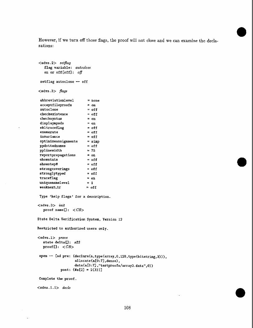
However, if we turn off those flags, the proof will not close and we can examine the decla- rations:
<sdvs. 2> setflag flag variable: autoclose on or off[off]: off
setflag autoclose — off
<sdvs. 3> flags
abbreviationlevel = none
acceptfileproofs = on
autoclose = off
checkexistence = off
checksyntax = on
displaympsds = on
ekltraceflag = off enumerate = off
invariance = off
opt imizeassignments = simp
ppdottednames = off
pplinewidth = 75
reportpropagat ions = on showstats = off showstep# = off
strongcoverings = off
stronglytyped = off
traceflag = on
uniquenamelevel = 1
weaknext_.tr = off
Type 'help flags' for a description.
<sdvs.3> init proof name [] : < CR>
State Delta Verification System, Version 12
Restricted to authorized users only.
<sdvs.l> prove state delta.] : s22 proof [] : < CR>
open-- [sd pre: (declare(a,type(array,0,128,type(bitstring,3))), allocate(a[0:7].dense), data(a[0:7],"testproofs/array2.data",0))
post: (#a[2] = 2(3))]
Complete the proof.
<sdvs. 1. 1> decls
108

a[2] type(bitstring,3)
a type(array,0,128,type(bitstring,3))
<sdvs.l.l> simp expression: .a[2] = 2(3)
true
<sdvs. 1. 1> close
close — 0 steps/applications
2.9.6 Negate
The proofs involving negation can be run by typing eval (runtestproofs *negation-tests*). They include proofs of negations of state deltas by contradiction and also proofs that use the negate command.
The negate command asserts the negation of a specified state delta, via the equivalence (in the case where Q does not have any top-level dots or quantifiers) between
" [sd pre: P comod: C
mod: M post: Q]
and
[sd pre: true comod: all
mod: all - C post: P(#/.) &
[sd pre: true comod: all - M mod: ()
post: "Q]3
if the state delta is known to be false (see [30]). (For the case when the state delta has invariants, see Section 8.4.)
For example, consider the state delta negateö.sd:
[sd pre: ("(([sdpre: (p) comod: (c) mod: (m) post: (q)]))) post: ("(([sdpre: (true) comod: (c) mod: (m) post: (q)])))]
Below is a transcript of the proof session:
109

<sdvs.l> prove state delta[]: negateß.sd proof []: <CR>
open — [sd pre: ("(([sdpre: (p) comod: (c) mod: (m) post: (q)]))) post: (~(([sd pre: (true)
comod: (c) mod: (m)
post: (q)])))]
Complete the proof.
<sdvs.l.l> usable
No usable state deltas.
No usable quantified formulas.
<sdvs.l.l> cases case predicate: ~([sdpre: (true) comod: (c) mod: (m) post: (q)J)
cases — "(([sd pre: (true) comod: (c) mod: (m) post: (q)]))
open — [sdpre: ("(([sdpre: (true) comod: (c) mod: (m)
post: (q)]))) comod: (all) post: (~(([sd pre: (true)
comod: (c) mod: (m)
post: (q)])))]
close — 0 steps/applications
open — [sd pre: (~(("(([sd pre: (true) comod: (c) mod: (m)
post: (q)]))))) comod: (all) post: (~(([sd pre: (true)
comod: (c) mod: (m)
post: (q)])))]
Complete the proof.
<sdvs.l.l.2.1> usable
u(l) [sd pre: (true) comod: (c) mod: (m) post: (q)]
u(2) [sd pre: ("(([sd pre: (true) comod: (c) mod: (m) post: (q)]))) comod: (all)
post: ("(([sdpre: (true) comod: (c) mod: (m) post: (q)])))]
110

No usable quantified formulas.
<sdvs. 1.1.2. 1> negate state delta: [sd pre: (p) comod: (c) mod: (m) post: (q)] formula name #1: fmll
negated result — [sd pre: (true) comod: (all) mod: (diff(all,c))
post: (p, [sd pre: (true)
comod: (diff(all.m)) post: ("q)])]
<sdvs.1.1.2.2> pp object: fmll
formula fmll: [sd pre: (true) comod: (dif f (all ,m) ) post: ("q)]
<sdvs.l.l.2.2> usable
u(l) [sd pre: (true) comod: (all)
mod: (diff(all,c)) post: (p,
[sd pre: (true) comod: (diff(all,m)) post: (~q)])]
u(2) [sd pre: (true) comod: (c) mod: (m) post: (q)]
u(3) [sd pre: ("(([sd pre: (true) comod: (c) mod: (m) post: (q)]))) comod: (all) post: (~(([sd pre: (true) comod: (c) mod: (m) post: (q)])))]
No usable quantified formulas.
<sdvs. 1.1.2. 2> apply sd/number[highest applicable/once]: u
number: 1
apply — [sd pre: (true) comod: (all)
mod: (diff(all,c)) post: (p,
[sd pre: (true) comod: (diff(all,m)) post: (~q)])]
Warning: the modlist of the last applied state delta mentions places
111

(diff(all,c)) outside of the modlist of the state delta to be proven. The current proof can only be closed by contradiction.
<sdvs.l.l.2.3> usable
u(l) [sd pre: (true) comod: (diff(all.m)) post: (~q)]
u(2) [sd pre: (true) comod: (c) mod: (m) post: (q)]
No usable quantified formulas.
<sdvs.l.l.2.3> apply sd/number[highest applicable/once]: u
number: 2
inserting — pcovering(all,m)
apply — [sd pre: (true) comod: (c) mod: (m) post: (q)]
Warning: the modlist of the last applied state delta mentions places (m) outside of the modlist of the state delta to be proven. The current proof can only be closed by contradiction.
inserting — pcovering(all,m)
<sdvs.l.l.2.4> usable
u(l) [sd pre: (true) comod: (diff(all,m)) post: (~q)]
No usable quantified formulas.
<sdvs.l.l.2.4> apply sd/number[highest applicable/once]: u
number: 1
apply — [sd pre: (true) comod: (diff(all,m)) post: (~q)]
The postcondition of the last applied state delta is inconsistent with the current state.
close — 3 steps/applications
join — [sd pre: (true) comod: (all) post: (~(([sd pre: (true)
comod: (c) mod: (m)
112

post: (q)])))]
close — 1 steps/applications
Here is another example, also illustrating that formulas can be negated:
<sdvs.l> pp object: tobeneg
formula tobeneg: [sd pre: (true) comod: (all) post: (p)]
<sdvs.l> pp object: negged.sd
[sd pre: ("(formula(tobeneg))) comod: (all) post: (~p)]
<sdvs.l> prove state deltaG : negged.sd proof []: <CR>
open — [sd pre: ("(formula(tobeneg))) comod: (all) post: (~p)]
Complete the proof.
<sdvs.l.l> usable
No usable state deltas.
No usable quantified formulas.
<sdvs. 1. 1> negate state delta: [sd pre: (true) comod: (all) post: (p)] formula name #1: fml2
negated result — [sd pre: (true) comod: (all)
mod: (diff(all,all)) post: (true,
[sd pre: (true) comod: (all) post: ("p)])]
<sdvs. 1. 2> usable
u(l) [sd pre: (true) comod: (all)
mod: (diff(all,all))
113

post: (true, [sd pre: (true) comod: (all) post: ("p)])]
No usable quantified formulas.
< sdvs. 1. 2> apply sd/number [highest applicable/once] : < CR>
apply — [sd pre: (true) comod: (all)
mod: (diff(all.all)) post: (true,
[sd pre: (true) comod: (all) post: (~p)])]
<sdvs.l.3> usable
u(l) [sd pre: (true) comod: (all) post: (~p)]
u(2) [sd pre: (true) comod: (all)
mod: (diff(all,all)) post: (true,
[sd pre: (true) comod: (all) post: (~p)])]
No usable quantified formulas.
<sdvs. 1. 3> apply sd/number [highest applicable/once]: <CR>
apply — [sd pre: (true) comod: (all) post: ("p)]
close — 3 steps/applications
2.9.7 Linearize
Linearize is the command intended to take two usable state deltas Si and S2 having true preconditions and form the disjunction of two state deltas: the first claiming that 5X : post occurs first in the future and then S2 : post, and the second claiming that S2 : post occurs first and then Si : post. In both cases the modlist in force until the first postcondition is achieved is the intersection of Si : mod and S2 : mod. The possible simultaneous occur- rence of both postconditions is allowed in either case. This situation corresponds to the interleaving of two parallel program fragments. For a discussion of linearize in the presence
114

of invariants, see Section 8.2.
For example, consider the state delta incboth:
[sd pre: (covering(all.x.y), .x = 0,.y = 0,formula(incx),fonnula(incy)) comod: (all)
mod: (all) post: (false)]
where incx and incy are as follows:
[sd pre: (true) mod: (x) post: (#x =1)]
[sd pre: (true) mod: (y) post: (#y = 1)]
This state delta is true because the two interior state deltas in the precondition are contra- dictory with the covering statement. The linearize command gives us the means to force the system to recognize this contradiction by making one of the postconditions true with a mod list equal to the intersection of the mod lists of the linearized state deltas. This intersection is empty, and thus neither x nor y can change value.
<sdvs.l> prove state delta D: incboth proof []: <CR>
open — [sd pre: (covering(all,x,y),.x = 0,.y = 0,formula(incx), formula(incy) )
comod: (all) mod: (all)
post: (false)]
Complete the proof.
<sdvs. 1. 1> usable
u(l) [sd pre: (true) mod: (y) post: (#y = 1)]
u(2) [sd pre: (true) mod: (x) post: (#x = 1)]
No usable quantified formulas.
<sdvs. 1. 1> linearize state delta #1: u
number: 1 state delta #2: u
number: 2 formula name #1: incy
115

formula name #2: incx
linearize — fommla(incy) or formula(incx)
non-trivial propagations — ([sd pre: (true) comod: (all) mod: (inter(y.x))
post: (#y = 1, [sd pre: (true) comod: (all) mod: (x)
post: (#x = 1)])]) or ([sd pre: (true)
comod: (all) mod: (inter(y.x))
post: (#x = 1, [sd pre: (true)
comod: (all) mod: (y)
post: (#y = 1)])])
<sdvs. 1. 2> cases case predicate: [sd (true) (all) (inter(y, x)) (#y = 1, [sd (true) (all) (x) (#x = 1)])]
cases — [sd pre: (true) comod: (all) mod: (inter(y,x))
post: (#y = 1, [sd pre: (true) comod: (all) mod: (x)
post: (tx = 1)])]
open — - [sd pre ([sd pre (true) comod (all) mod (inter(y,x))
post (#y = 1, [sd pre: (true) comod: (all) mod: (x)
post: (#x = 1)])]) comod- (all) mod: (all)
post: (false)]
<sdvs.l.2.1.1> usable
u(l) [sd pre: (true) comod: (all)
mod: (inter(y, x)) post: (*y = 1,
[sd pre: (true) comod: (all)
mod: (x) post: (#x = 1)])]
116

u(2) [sd pre: (true) mod: (y) post: (#y =1)]
u(3) [sd pre: (true) mod: (x) post: (#x = 1)]
No usable quantified formulas.
<sdvs.l.2.1.1> apply sd/iiumber[highest applicable/once]: <CR>
apply — [sd pre: (true) comod: (all) mod: (inter(y,x))
post: (#y = 1, [sd pre: (true) comod: (all)
mod: (x) post: (#x = 1)])]
The postcondition of the last applied state delta is inconsistent with the current state.
close — 0 steps/applications
open — [sd pre: ("(([sdpre: (true) comod: (all)
mod: (inter(y,x)) post: (#y = 1,
[sd pre: (true) comod: (all)
mod: (x) post: (#x = 1)])])))
comod: (all) mod: (all)
post: (false)]
Complete the proof.
<sdvs.l.2.2.1> usable
u(l) [sd pre: (true) comod: (all)
mod: (inter(y.x)) post: (#x = 1,
[sd pre: (true) comod: (all)
mod: (y) post: (#y = 1)])]
u(2) [sd pre: ([sd pre: (true) comod: (all) mod: (inter(y.x))
post: (#y = 1, [sd pre: (true)
117

comod: (all) mod: (x)
post: (#x = 1)])]) comod: (all)
mod: (all) post: (false)]
u(3) [sd pre: (true) mod: (y) post: (#y = 1)]
u(4) [sd pre: (true) mod: (x) post: (#x =1)]
No usable quantified formulas.
<sdvs. 1.2.2.1> apply sd/number[highest applicable/once]: <CR>
apply — [sd pre: (true) comod: (all)
mod: (inter(y.x)) post: (#x = 1,
[sd pre: (true) comod: (all) mod: (y)
post: (#y = 1)])]
The postcondition of the last applied state delta is inconsistent with the current state.
close — 0 steps/applications
join — [sd pre: (true) comod: (all) mod: (all) post: (false)]
close — 2 steps/applications
The postcondition of the last applied state delta is inconsistent with the current state.
2.9.8 Natural Number Induction
Natural number induction, or what is commonly referred to as "mathematical induction," was incorporated into SDVS 10 specifically to help overcome a hurdle in the proof of a sorting program; see [38].
The command can be used to prove claims of the form Vna{n), where n is assumed to range over the natural numbers. The command simply requests the user for the induction expression (n above), the formula (a(n')), the base proof, and the step proof. The proofs, as in other similar commands, can be left empty at the time of the command invocation, and supplied interactively during the continuation of the proof. The base-case state delta claims that the formula is true for n = 0, i.e., o(0), and the step-case state delta claims that if the formula is true for n, then it is true for n + 1.
118

As a simple example, we prove that Vn(n + 1 > n). The proof closes automatically.
<sdvs.l> natinduct induction expression: n
formulas: n-f-1 gt n base proof [] : < CR> step proof [] : < CR>
natural induction on n — (n + 1 gt n)
open — [sd pre: (n = 0) comod: (all) post: (n + 1 gt n)]
close — 0 steps/applications
open — [sd pre: (n ge 0,n + 1 gt n) comod: (all) post: ((n + 1) + 1 gt n + 1)]
close — 0 steps/applications
join natural induction cases — forall n (n ge 0 —> n + 1 gt n)
2.9.9 Mapping
The proof language must allow the user to specify the mapping (correspondence) between the places of one state delta and another state delta that implements it, or, more generally, between the states of one computation and another that implements it. For a more detailed treatment of mapping, see [39].
A mapping is an assignment for each target (upper level) place of a set of host (lower level) places such that the value of the target place is a function of the values of the associated host places. A technicality forces the requirement that this function must be one-to-one if the target place appears in the comodification list of a target state delta. However, the user does not have to worry about this, since the implementation command does not allow nonempty comodification lists in the upper level at all. Three types of statements must be proved about the mapping:
1. Disjointness among a set of target places must be reflected in the disjointness of the associated sets of host places.
2. Declarations of the target places (length of bitstrings, or range of arrays) must be proved from the declarations associated with the corresponding host places.
3. The translations of the target state deltas into the host language induced by the mappings must be proved from the host description.
119

The command implementation fills the role of "theorem constructor." It takes (or prompts the user for) a theorem name, the upper-level specification, the lower-level specification, the formula containing the mapping functions, the places in the host that must be constant for the implementation to be valid, and the invariants for host state changes that must hold for the implementation to be valid.
The result is a theorem (state delta) that denotes the implementation of the upper level by the lower level. The precondition of the theorem contains the lower-level specification, the constant formulas, and some equalities that provide names for certain sets of places in the lower level, specifically,
1. names for the set of all lower-level places,
2. the set of all mapped lower-level places,
3. the set of all unmapped lower-level places, and
4. the set of all constant lower-level places.
The comod and mod of the theorem are empty. The postcondition of the theorem contains n+2 items, where there are n state deltas in the upper-level specification. The first item is an alldisjoint predicate stating the disjointness of the sets of mapped-onto lower-level places. The second item is a state delta representing the validity of the upper-level declarations and the one-to-oneness of certain mapping functions. The next n items are upper-level state deltas that have been transformed into lower-level theorems.
The mapping construct can take either the form
1. mapping(.tplace, f^hplace!, ..., .hplacen)), where f is some explicit function, e.g. mapping(.tplace, .hplace), or
2. mapping(.tplace, f(.hplace1: ..., .hplacen),values(tval1,f(hval11, ..., hvaln1), ... tvalk,
f(hvalik, ..., hvalmk))), where the tvals are possible values of tplace and the hvals are
possible values of the hplaces.
The constant field can take four kinds of statements:
1. constant(.p), expressing the fact that .p is constant, but we do not know or care what that value is;
2. .p = c, the actual value that does not change;
3. data(.p[i:j], file, offset), for values of arrays (here is where the ROMs for microprograms could be initialized); or
120

4. allocate statements to accompany the data statements.
The invariants field takes a fornrala or list of formulas. The invariants field, if needed, is used to specify the significant states in the lower-level machine. In other words, sometimes the mapping of places to places as specified by the mapping formula is not sufficiently rich to induce the state-to-state mapping required by the implementation theorem. Invariants must hold for every lower-level state, including the initial state. They are usually implications of the following form: if certain mapped places have certain values, then other conditions must hold.
As an example, consider the following simple case:
First, the lower-level machine, the host machine alOisp:
machinea:=( »»Registers**
a<l:0>
»»Process**
cycleajmain}:=
begin a_l next a_0 end )
<sdvs.l> ppsd state delta: isps
file name: alO.isp
covering(machinea,a,machinea\upc) declare(a,type(bitstring,2)) [tr 8MACHTNEA\STARTED {in MACHINEA} A ; A ;]
Now, the upper-level machine, the target machine bO.isp:
machineb:=( »♦Registers**
b<l:0>
»♦Process**
cycleb{main}:=
begin b_0 end )
121

You need to mpisps the file and then you may look at the result (although it is not necessary to ppsd it):
<sdvs.2> ppsd state delta: mpisps
file name: bO.isp starting mark point D : <CR> ending mark pointsD : <CR>
preconditionsD : <CR>
covering(machineb,b,machineb\upc) declare(b.type(bitstring,2)) [sd pre: (.machineb\upc = machineb\started)
mod: (b,machineb\upc) post: (#machineb\upc = machineb\halted,#b = 0(2))]
Here is the mapping specification from target places to host places:
<sdvs.2> pp object: bOalO.mapping
formulas bOalO.mapping: mapping(.b,.a)
mapping (.machineb\upc,map\upc(.machinea\upc), values(machineb\started,
map\upc(machinea\started), machineb\halted, map\upc(machinea\halted)))
Next, we invoke the implementation command (after having mpispsed bO.isp and ispsed alO.isp; for more information about mpisps, see page 145):
<sdvs.2> implementation theorem name: bOalO.thm
upper-level spec: mpisps file name: bO.isp
starting mark point [] : <CR> ending mark points 0: < CR>
precondit ions □ : < CR> lower-level spec: isps
file name: alO.isp mappings: formulas (bOalO. mapping)
const ant s [] : < CR> invariants [] : < CR>
Implementation theorem 'bOalO.thm' created.
Here is the theorem (formula) that was created:
122

<sdvs.2> pp object: bOalO.thrn
[sd pre: (isps(alO.isp).bOalO.thm.places = union(a,machinea\upc), bOalO.thrn.mapped.places = union(a,machinea\upc), bOalO.thm.unmapped.places
= diff(bOalO.thm.places,bOalO.thrn.mapped.places)) post: (alldisjoint(a,machinea\upc),
[sd pre: (true) comod: (all) post: (forall al (lh(al) = 2 —> lh(al) = 2))],
[sd pre: (.machinea\upc = machinea\started) mod: (a,machinea\upc,bOalO.thm.unmapped.places)
post: (#machinea\upc = machinea\halted,#a = 0(2))])]
Make sure to use the formulas construct around the mapping name (the mappings have already been defined). Note that the three clauses in the postcondition correspond to the three types of statements above. Now let us prove it.
<sdvs. 2> prove state deltaD: bOalO.thrn proof []: <CR>
open— [sd pre: (isps(alO.isp), bOalO.thrn.places = union(a,machinea\upc), bOalO.thm.mapped.places = union(a,machinea\upc), bOalO.thm.unmapped.places
= diff(bOalO.thm.places,bOalO.thrn.mapped.places)) post: (alldisjoint(a,machinea\upc),
[sd pre: (true) comod: (all) post: (forall al (lh(al) = 2 —> lh(al) = 2))],
[sd pre: (.machinea\upc = machinea\started) mod: (a,machinea\upc,bOalO.thrn.unmapped.places)
post: (#machinea\upc = machinea\halted,#a = 0(2))])]
Complete the proof.
<sdvs.2.1> whynotgoal simplify? [no]: <CR>
g(2) [sd pre: (true) comod: (all) post: (forall al (lh(al) = 2 --> lh(al) = 2))]
g(3) [sd pre: (.machinea\upc = machinea\started) mod: (a,machinea\upc,bOalO.thrn.unmapped.places)
post: (#machinea\upc = machinea\halted,#a = 0(2))]
<sdvs. 2. 1> prove state deltaD : g
number: 3 proof [] : < CR>
123

open — [sd pre: (.machinea\upc = machinea\started) mod: (a,machinea\upc,bOal0.thm.unmapped.places)
post: (#machinea\upc = machinea\halted,#a = 0(2))]
Complete the proof.
<sdvs.2.1.1> until formula: #machine\upc = machine\halted
apply — [sd pre: (.machinea\upc = machinea\started) mod: (machinea\upc,a)
post: (#a = 1(2), [tr {in MACHMEA} A ;])]
apply — [sd pre: (true) comod: (machinea\upc) mod: (machinea\upc,a)
post: (#a = 0(2), [tr 6MACHINEA\halted])]
apply — [sd pre: (true) comod: (machinea\upc)
mod: (machinea\upc) post: (#machinea\upc = machinea\halted)]
close — 3 steps/applications
Complete the proof.
<sdvs.2.2> whynotgoal simplify? [no] : < CR>
g(2) [sd pre: (true) comod: (all) post: (forall al (lh(al) = 2 —> lh(al) = 2))]
<sdvs.2.2> prove state delta[] : g
number: Z proof [] : < CR>
open — [sd pre: (true) comod: (all) post: (forall al (lh(al) = 2 —> lh(al) = 2))]
close — 0 steps/applications
close — 2 steps/applications
<sdvs.3> ps
« initial state >> mpisps testproofs/bO.isp <2> proved bOalO.thm <1> —> you are here <—
124

2.9.10 Formulas
The command formulas (<name-of-list-of-exprs>) will insert the list of formulas associated with the name. It is useful when a long hypothesis occurs in more than one state delta.
The command formula(<expr-name>) inserts the single formula associated with the <expr- name>. One may also insert state deltas by using formula(<sd-name>).
<sdvs. 1> createformula name: hyp2
formula: .a = 5
<sdvs. 1> createsd name: flO.sd
[SD pre: .a = 5 comod[]: <CR>
mod [] : all post: #a = 10
]
<sdvs. 1> createsd name: fl4-sd
[SD pre: formulafflO.sd), formula(hyp2) comod[]: <OR>
mod [] : all post: #a = 10
]
<sdvs.l> prove state delta[] : fl4-sd proof D: <CR>
open— [sd pre: (formulaCflO.sd),formula(hyp2)) mod: (all)
post: (#a = 10)]
inserting — pcovering(all,a)
Complete the proof.
<sdvs.l.l> usablesds
u(l) [sd pre: (.a = 5) mod: (all)
post: (#a = 10)]
<sdvs. 1. 1> apply sd/number[highest applicable/once]: <CR>
apply — [sd pre: (.a = 5) mod: (all)
post: (#a = 10)]
125

close — 1 steps/applications
<sdvs.2> createformulas name: hypS
formula list: .a = 1, .a = 2
<sdvs.2> pp object: hypS
formulas hyp3: .a = 1 .a = 2
<sdvs. 2> createsd name: fl5.sd
[SD pre: formulas (hypS) comod[]: <CR>
mod[]: all post: false
]
<sdvs. 2> init proof name D : < CR>
State Delta Verification System, Version 11
Restricted to authorized users only.
<sdvs.l> prove state delta[]: fl5.sd proof []: <CR>
open — [sd pre: (formulas(hyp3)) mod: (all)
post: (false)]
The state delta is vacuously TRUE because its precondition is FALSE.
close — 0 steps/applications
Here is another example illustrating the disjunction of formulas and using a state delta as a case predicate.
<sdvs.l> pp object: queue
formula queue: q
<sdvs.l> pp object: disj.formula.sd
[sd pre: (formula(tobeneg) or formula(queue)) mod: (all)
post: (p or q)]
126

<sdvs.l> prove state delta[]: disj.formula.sd proof []: <CR>
open — [sd pre: (formula(tobeneg) or formula(queue)) mod: (all)
post: (p or q)]
non-trivial propagations — ([sd pre: (true) comod: (all) post: (p)]) or
q
Complete the proof.
<sdvs.l.l> usable
No usable state deltas.
No usable quantified formulas.
<sdvs. 1. 1> cases case predicate: [sd pre: (true) comod: (all) post: (p)]
cases — [sd pre: (true) comod: (all) post: (p)]
open — [sd pre: ([sd pre: (true) comod: (all) post: (p)])
comod: (all) mod: (all)
post: (p or q)]
<sdvs.l.l.l.l> usable
u(l) [sd pre: (true) comod: (all) post: (p)]
No usable quantified formulas.
<sdvs.l.l.l.l> apply sd/number[highest applicable/once]: <CR>
apply — [sd pre: (true) comod: (all) post: (p)]
close — 1 steps/applications
open — [sd pre: ("(([sdpre: (true) comod: (all) post: (p)])))
comod: (all) mod: (all)
post: (p or q)]
127

close — 0 steps/applications
join — [sd pre: (true) comod: (all)
mod: (all) post: (p or q)]
close — 1 steps/applications
2.9.11 Macros
The macro facility is essentially a parametrized formula of the preceding section. This capability was initially developed to aid in the quicksort proof (see [38]). A macro is a named formula (possibly quantified) with designated lists of free and quantified variables (possibly NIL). It is defined by the command createmacro(name)(free variables)(quantified variables). It is invoked by the term name(subs), where subs is a list of terms corresponding to the declared variables, both free and quantified, in one contiguous sequence separated by commas. The characteristic distinguishing between the substitutions corresponding to the free variables and those corresponding to the quantified variables is that the latter can be only names (atoms), not arbitrary terms. When invoked, the correct substitutions are performed and the resulting formula is inserted in place of the macro.
As an example, consider the macro sorted and the state delta sorted.sd, exhibited below.
<sdvs.l> createmacro name: sorted
pattern: forall i (1 le i and i It range(a) -> .a[i:i] le .a[i+l:i+l]) free variables □ : a
quantifier symbols[] : t
<sdvs.l> pp object: macro macro name: sorted
macro sorted (a),(i): forall i (1 le i ft i It range(a) —> .a[i:i] le .a[(i + l):(i+ 1)])
<sdvs.l> pp object: sorted.sd
[sd pre: (sorted(x.i)) post: (sorted(x[j:k],i))]
<sdvs.l> prove state delta[] : sorted.sd proof [] : usable
open — [sd pre: (sorted(x.i)) post: (sorted(x[j:k],i))]
No usable state deltas.
128

q(l) forall i (1 le i & i It range(x) —> .x[i:i] le .x[(i + l):(i + 1)])
Complete the proof.
<sdvs.l.l> goals
g(l) forall i (1 le i & i It range(xCj:k]) —> .x[j:k][i:i] le .x[j:k][(i + l):(i+ 1)])
At this point, the macro has been invoked and the problem is reduced to a simple question of proving a state delta (which we do not bother to do here).
2.9.12 Composition of State Deltas
Composition is the method for combining the effect of the sequential execution of several state deltas into one state delta. The command is called compose. Composition is used internally in processing mpisps and vhdltr, and it can also be called explicitly by the user in interactive mode. Here is an example illustrating an arithmetic swap.
<sdvs.l> compose composed sd name: swapcompose.sd
Do you ¥ish to compose sds from the proof stack? (y or n) [n] : n [sd (true) (all) (x) (#x = .x + .y)] [sd (true) (all) (y) (#y = .x - .y)] [sd (true) (all) (x) (#x = .x - .y)] <CR> covering(all, x, y)
sd D sd [] sd D sd []
declarations []
Experimental Composer
Composed
[sd pre: (true) mod: (y,x)
post: (#x = .y,#y = -x)]
For a more detailed look at composition, see
The following example illustrates the use of composition in a proof of the state delta c5.sd:
<sdvs.l> pp object: c5.sd
[sd pre: (covering(all,x,y,upc,tmp) .formulas(machine) , .upc = 1) mod: (all)
post: (#x = .x + l,#y = .y)]
129
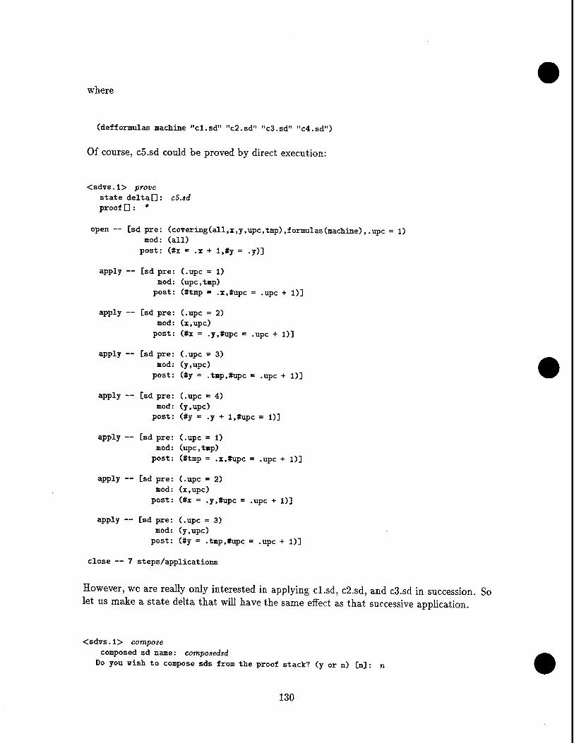
where
(defformulas machine "cl.sd" "c2.sd" "c3.sd" "c4.sd")
Of course, c5.sd could be proved by direct execution:
<sdvs.l> prove state deltaQ: c5.sd proof [] : *
open— [sd pre: (covering(all,x,y,upc,tmp).formulas(machine),.upc = 1) mod: (all)
post: (#i = .x + l,#y = .y)]
apply — [sd pre: (.upc = 1) mod: (upc.tmp)
post: (#tmp = .x,#upc = .upc + 1)]
apply — [sd pre: (.upc = 2) mod: (x.upc)
post: (#x = .y,«upc = .upc + 1)]
apply — [sd pre: (.upc = 3) mod: (y,upc)
post: (#y = .tmp.tupc = .upc + 1)]
apply — [sd pre: (.upc = 4) mod: (y.upc)
post: (#y = .y + l,#upc = 1)]
apply — [sd pre: (.upc = 1) mod: (upc.tmp)
post: (#tmp = .x,#upc = .upc + 1)]
apply — [sd pre: (.upc =2) mod: (x.upc)
post: (#x = .y,#upc = .upc + 1)]
apply — [sd pre: (.upc = 3) mod: (y.upc)
post: (#y = .tmp,#upc = .upc + 1)]
close — 7 steps/applications
However, we are really only interested in applying cl.sd, c2.sd, and c3.sd in succession. So let us make a state delta that will have the same effect as that successive application.
<sdvs. 1> compose composed sd name: composedsd
Do you wish to compose sds from the proof stack? (y or n) [n]: n
130

sd []: cl.sd sd []: c2.sd sd []: cS.sd sd []: <CR>
declarations[] : covering(all, x, y, tmp, upc)
Experimental Composer
Composed
[sd pre: (.upc = 1) mod: (x,tmp,y,upc)
post: (#upc = 4,#y = .x,#x = .y,#tmp = .x)]
Now we can use the following as a proof:
(defproof example "(prove c5.sd proof:(prove composedsd
proof: (apply cl.sd, apply c2.sd, apply c3.sd, close),
apply composedsd, apply c4.sd, apply composedsd, close))")
Notice that composedsd will have to be proved before it can be applied. Every state delta resulting from the compose command should be provable by *. The <declarations> field can be only a covering or declaration statement.
<sdvs.l> init proof name [] : example
State Delta Verification System, Version 11
Restricted to authorized users only.
open— [sd pre: (covering(all,x,y,upc,tmp).formulas(machine),.upc = 1) mod: (all)
post: (#x = .x + l,#y = .y)3
open — [sd pre: (.upc =1) mod: (x,tmp,y,upc)
post: (»upc = 4,#y = .x,#x = .y.ttmp = .x)]
apply — [sd pre: (.upc =1) mod: (upc,tmp)
post: (#tmp = ,x,#upc = .upc + 1)]
131

apply — [sd pre: (.upc = 2) mod: (x,upc)
post: (#x = .y,#upc = .upc + 1)]
apply — [sd pre: (.upc = 3) mod: (y.upc)
post: (#y = .tmp,#upc = .upc + 1)]
close — 3 steps/applications
apply — [sd pre: (.upc = 1) mod: (x,tmp,y,upc)
post: (»upc = 4,#y = .x,#x = .y,#tmp = .x)]
apply — [sd pre: (.upc = 4) mod: (y.upc)
post: (#y = .y + l,#upc = 1)]
apply — [sd pre: (.upc =1) mod: (x,tmp,y,upc)
post: (#upc = 4,#y = .x,#x = .y,#tmp = .x)]
close — 4 steps/applications
2.9.13 The SDVS Language Parser
Internally, SDVS deals with expressions in prefix notation, e.g. (USSUB X 7 0). The prettyprinter will print this expression in infix notation as X<7:0>. Those operators that have different infix and prefix symbols (such as "plus" and "+") maybe input interactively either in infix or in mathematical (not Lisp) prefix notation, in any combination. Some operators have only one symbol for both the infix and the prefix notation (such as "It," since the character < is reserved for substring selection). Some operators have only a mathematical prefix form, such as the enumeration type relations and queueing operations. SDVS is not case sensitive.
For example,
<sdvs.l> createsd name: sd5
[SD pre: covering(all, a), eq(plus(x, y), 1) comod[]: <CR>
mod[]: <CR> post: pound(a) = .a + 1
]
<sdvs.l> ppsd state delta: sd5
[sd pre: (covering(all,a),x + y = 1) post: (#a = .a + 1)]
132

It is essential to parenthesize expressions that may be ambiguous, for example p -> q or r. Otherwise, they may be interpreted differently than intended, with unpredictable results.
Some symbols may be typed in at the terminal in their prettyprinted format, some must be typed in in their non-prettyprinted format, and some may be typed in either way. For example:
<sdvs.l> simp expression: a or b
a or b
<sdvs.l> simp expression: a and b
a ft b
<sdvs.l> simp expression: a & b
a ft b
The infix-prefix correspondence (for those operators with both forms) is as follows:
prefix infix
aconc aconc
abs abs and &
div /
dot . eq =
exists 3 expt ~*
forall V ge ge
g* gt implies —> (input),
invert
le le In In It It minus -
mult *
neq "= (input),
not **
(prettyprinted)
133

ones ones
or or (input), V (prettyprinted) plus + pound # rem rem us and && uscone @ usdifference — useql ==
usgeq usge
usgtr usgt usleq usle uslss uslt usneq "== usnot """
us or usor (input), VV (prettyprinted) usplus ++ usquotient // usremainder usmod
ustimes ** usxor usxor zeros zeros
Nonstandard transformations:
(usval X) (cond ABC) (bs X Y) (ussub A X Y) (element A X) (slice A X Y)
IXI (if A then B else C) X(Y) A<X:Y> A[X] A[X:Y]
The following is a list of reserved words, other than commands and the standard interpreted function symbols, that have special meaning in SDVS and should not be used in other than their official capacity.
all
constant
covering
declaration
diff
inter
map
134

pcovenng sd sdtobeproven
tr union
2.9.14 Reading, Writing, and Editing
The commands read and write are the SDVS input-output commands for user-created files. Write prompts the user for the names of all objects that can possibly be stored (e.g. state deltas and proofs). SDVS converts all the objects into the def form, e.g. defproof, which can then be edited as desired. Äearfgoes to the designated file and processes all the de/forms.
<sdvs.l> write path name[lemmas/lemmas.lemmas]
state delta names [] proof names [] axiom names [] lemma names []
formula names [] formulas names []
macro names [] datatype names [] adalemma names []
junk <CR> <CR> <CR> <CR> <CR> <CR> <CR> <CR> <CR>
Do you wish to append to the already existing file? n
No objects written.
The primary method for creating proofs interactively is simply to type in proof commands in an SDVS proof session. The proof can then be named by the dump-proof command (see be- low) and written to a file. Another method is to use the command createproof. For example,
<sdvs. 1> createproof name: testproof
proof: (prove [sd pre: (p) comod: () mod: () post: (true)] proof: ())
<sdvs.l> pp ob j ect: testproof
proof testproof:
prove [sd pre: (p) post: (true)] proof:
The proper constructors for use in the editor, corresponding to the interactive create con- structs, are defproof, defsd, and defformulas.
135

The form in which these definitions can be evaluated in the editor is
(defitem <itemname> ''<itembody>'')
A common situation arises when the user has finished an interactive proof, SDVS has collected this into sdvsproof, and the user would like to change the name. The easiest way to do this is to use the dump-proof command. Another way, which might be useful under certain circumstances, is to write the proof to a file using the write command, change the name in the editor, and then evaluate the defsd.
For example,
(defproof casesproof "(prove [sd pre: ([sd pre: (pi ft p2) mod: (all)
post: (ql)], [sd pre: (pi ft "p2)
mod: (all) post: (q2)],
[sd pre: (~pl ft p2) mod: (all)
post: (q2)], [sd pre: ("pi ft "p2)
mod: (all) post: (ql)])
mod: (all) post: (ql or q2)]
proof: meases
(case: pi ft p2 proof: * case: pi ft ~p2 proof: *
case: ~pl ft p2 proof: * case: "pi ft ~p2 proof: *))")
If the state delta exists in unparsed (input) notation in the editor, say as
[sd ...]
it may be input into SDVS by typing in the editor
(defsd sdname "[sd ...]")
and then evaluating.
If defproof does not work on some proof, putproof may be used. The differences are that in putproof, the name of the proof and the proof itself must be single quoted, and with
136

defproof the proof must be string quoted. Also, in putproof, the proof itself is given in Lisp notation, whereas defproof takes the unparsed prettyprint version.
Also note that in using the defproof method, quotation marks around path names must be preceded by backslashes to appear as follows:
(defproof proof1 "(prove s22
proof: readaxioms \"axioms/bitstring.axioms\")")
For example, in case you wish to change the name of a proof, and the above defsd method does not work, do the following:
(putproof '<new-proofname> (proofp 'sdvsproof))
and then evaluate.
To summarize, the two methods of obtaining a proof are evaluating in Lisp
1. (proofp 'proofname) and
2. (get 'proofname 'proof)
Similarly, the two methods of obtaining a state delta named sdname are
1. (sdp 'sdname) and
2. (get 'sdname 'sd)
2.9.15 Batch Proofs
The user may write a batch proof in the editor by using the commands of the previous section, or may write it interactively by using the command createproof.
< sdvs. 1 > createproof name: tproof
proof: prove tests proof: (*, close)
Of course, the user may also type in the actual state delta in place of just giving its name, and may type in an arbitrarily long proof. However, given the complexity of the syntax and the probability of making an error, it is strongly recommended that the user modularize the work, or use the editor.
A batch proof may be run by typing its name at the prompt after the init command (if a clean system is needed), or after the interpret command (if it is desired to continue from the current context).
137

2.9.16 Disjunctions of State Deltas
Disjunctions of state deltas in preconditions are treated just like disjunctions of any other sentences. (Be sure that when typing in disjunctions of state deltas the state delta square brackets are enclosed by parentheses: ([sd ....]) or ([sd ....]).) To use a disjunction of state deltas, a proof by cases must be done:
<sdvs.l> ppsd state delta: intl.sd
[sd pre: (true) post: (q)]
<sdvs.l> ppsd state delta: intS.sd
[sd pre: (true) post: (r)]
<sdvs.l> ppsd state delta: s8
[sd pre: (formula(intl.sd) or formula(int2.sd)) post: (q or r)]
<sdvs.l> prove state delta[]: s8 proof []: <CR>
open — [sd pre: (formula(intl.sd) or formula(int2.sd)) post: (q or r)]
non-trivial propagations — ([sd pre: (true) post: (q)]) or
([sd pre: (true) post: (r)])
Complete the proof.
<sdvs.l.l> cases case predicate: formula(intl.sd)
cases — formula(intl.sd)
open — [sd pre: (formula(intl.sd)) comod: (all) post: (q or r)]
<sdvs.l.l.l.l> usable
u(l) [sd pre: (true) post: (q)]
No usable quantified formulas.
138

<sdvs.l.l.l.l> apply sd/number[highest applicable/once]: <CR>
apply — [sd pre: (true) post: (q)]
close — 1 steps/applications
open — [sd pre: ("(formula(intl.sd))) comod: (all) post: (q or r)]
Complete the proof.
<sdvs.l.l.2.1> usable
u(l) [sd pre: (true) post: (r)]
u(2) [sd pre: (formula(intl.sd)) comod: (all) post: (q or r)]
No usable quantified formulas.
<sdvs.l.l.2.1> apply sd/number [highest applicable/once]: <CR>
apply — [sd pre: (true) post: (r)]
close — 1 steps/applications
join — [sd pre: (true) comod: (all) post: (q or r)]
close — 1 steps/applications
2.9.17 System Commands
New to SDVS 11 are two commands - cd and pwd - that, when typed at the SDVS prompt, do the same as the UNIX commands of the same name, connect to a directory and print the name of the working directory. The command shell allows the user to enter UNIX commands at the prompt, and the command exit kills the currently running SDVS job. Exit is the same as doing bye in SDVS followed by (quit) in Lisp.
2.9.18 Errors
When the user (interactively) types a proof command that cannot be executed, an explana- tory message is generated. When this same error occurs in a batch proof, a "command error" is generated and the proof halts. The command lasterror returns the current error
139

message.
2.9.19 Breaks in SDVS
Although we are confident that SDVS will usually not "crash" under normal operation, there are still some instances where a determined (or unlucky) user can break the system. One example is given here:
< sdvs. 1 > createsd name: decsd8
[SD pre: declare(x, type(fn, .x)) comod[]: <CR>
mod[]: <CR> post: false
]
<sdvs.l> prove state delta[]: decsd8 proof []: <CR>
open — [sd pre: (declare(x,type(fn,.1))) post: (false)]
inserting — pcovering(all,x)
Complete the proof.
If at this point you were to simp x = .x, the control stack would overflow.
Some of the reading and writing commands still react ungracefully if you type in a partic- ularly nonsensical path name, for example.
There are surely more examples.
2.9.20 Bugs in SDVS
In addition to errors and breaks, there are, unfortunately, still bugs. This means, to reuse a phrase, that there are still some instances where a determined (or unlucky) user can prove false. It is reassuring when an automated proof succeeds, but the user should understand that success as an increase in confidence in the correctness of the theorem, not a fool-proof guarantee.
Here is an example of using self-reference to prove false:
<sdvs.l> ppsd state delta: self
140

[sd pre: (formula(self)) post: (false)]
<sdvs.l> ppsd state delta: foo
[sd pre: (true) post: (false)]
<sdvs.l> prove state deltaQ: foo proof []: <CR>
open — [sd pre: (true) post: (false)]
Complete the proof.
<sdvs. 1. 1> prove state deltaD : self proof []: <CR>
open — [sd pre: (formula(self)) post: (false)]
The state delta to be proven is already known to be TRUE.
close — 0 steps/applications
Complete the proof.
<sdvs. 1. 2> apply sd/number [highest applicable/once] : <CR>
apply — [sd pre: (formula(self)) post: (false)]
The postcondition of the last applied state delta is inconsistent with the current state.
close — 1 steps/applications
<sdvs.2> ps
« initial state » proved foo <1> —> you are here <—
An algorithm to detect the unsoundness of circular state delta definitions (see [33]) has been implemented, but is not yet part of the distributed SDVS.
141

3 INTERACTION WITH ISPS
3.1 TR: TRANSLATOR FROM ISPS TO STATE DELTAS
In SDVS the internal language for expressing computations is the state delta language; thus the programs and specifications must be written in, or converted to, state deltas for processing by SDVS. For programs that already exist in other, more common, languages, or for programs that are more easily written in other languages, the problem of how to translate accurately into the state delta language must be overcome. In the simplest cases this may be done manually. However, for "real" programs, and in order to eliminate possible inaccuracies in the translation, the task is too difficult to be left to the user; the slightest error in the translation could invalidate the connection between the proof (about state deltas) and the original claim (about a program in some other language).
This section describes the action of the translator TR on the machine description language ISPS. Subsequent chapters discuss the translation of Ada and VHDL.
In fact, there are two different versions of the translator from ISPS to state deltas. The more recent translator will be discussed only in the last section of this chapter. It is still to be considered experimental, although it will eventually replace the old translator. It has been generated by the same uniform method as the translators for Ada and VHDL, and recognizes a slightly larger piece of ISPS (it allows "don't care" digits, and bit order in bitstrings can be low to high).
The version of ISPS that the (old) translator (TR) recognizes differs from the version described in the ISPS Manual ([9]) in several respects. The first category of differences contains those aspects of the "official" ISPS that TR does not support (see Figure 3): these include parallelism and two's-complement arithmetic.
The second category of differences consists of extra features that SDVS needs for the im- plementation proof paradigm. For example, when one is not interested in implementing the action of all target places, some of the machine variables ("place" names) must be designated as significant and the others as auxiliary. The mapping is defined only on the designated significant places. Another useful feature is the capability to intersperse stan- dard ISPS code with state deltas. This can be used when one is not interested in the details of how a certain postcondition was brought about, but only in its effect, or in case that effect is not expressible in ISPS.
A complete description of Aerospace ISPS is given in the report ISPS for SDVS ([40]); the semantics of TR are described in [62], [10], and [41]; tests for static semantic errors are described in [41]; and problems with ISPS are described in [42].
143

• Bit declarations must be from high to low and have zero as the rightmost bit.
• Word declarations must be from low to high and have zero as the leftmost word.
• One-bit scalars must be declared with brackets, e.g. A<> (or A<0>), not A.
• The right-hand side of a mapping must have been declared prior to the mapping.
• In our implementation only scalar entities may be on the right-hand side of a mapping declaration. The left-hand entity may be either a scalar or an entire element of an array.
• The REQUIRE and DEFINE declarations are unsupported.
• Function formals and return value cannot be arrays.
• ";" is interpreted as if it were "NEXT," i.e., parallel action is unsupported.
• Except for arithmetic transfer, unsigned is the only arithmetic mode implemented, and is required at the ISPS-Declaration level for compatibility with C-MU ISPS. The TC qualifier is required on arithmetic transfer.
• "?" is not allowed as a constant digit.
• The RESUME and TERMINATE statements are not allowed.
• UNPREDICTABLE, STOP, NO.OP, LAST.ONE, and UNDEFINED are the only implemented predeclared entities. UNDEFINED is allowed only on the right-hand side of a transfer operation.
• The arithmetic relation TST is unimplemented.
• MAIN, US, and TC are the only allowable qualifiers, with TC allowable only in the context of transfer operations.
• The user definition of qualifers is unimplemented.
• Quoted strings after BEGIN/END are not allowed.
• There is no call by reference.
• Side-effect-causing operations on the left-hand side of any transfer operation are not permitted.
• Nonfunction, nonassignment expressions, e.g. A+B, cannot be statements.
• The right operand in shifts cannot be longer than the left operand.
• The array index out of bounds may cause errors.
Figure 3: ISPS Features not Implemented in TR
144

3.2 MARKING
SDVS does the processing necessary to turn an ISPS program into an equivalent state delta or set of state deltas. Thus, ISPS programs can be used in, or as, preconditions or postconditions of state deltas.
A very simple example was given in Section 1.9. A more complicated example illustrating the capability to execute from an ISPS mark point is shown next. One can run a set of example ISPS proofs by typing eval (runtestproofs *isps-tests*).
When dealing with a proof based on state deltas created by TR from an ISPS program, the user does not have a convenient method of handling the specific state deltas representing the "continuation" of the program from each control point. To solve that problem, the system allows the user to label the location of control points in the ISPS program.
The initial and final control points are named by the system <machine-name>\STARTED and <machine-name>\HALTED, respectively. The exit point for an internal subroutine, <subroutine>, is <subroutine>\exited.
Consider the following ISPS program:
gcd.machine US := BEGIN ! gcd algorithm computes gcd(x.y) ! for inputs x and y
** local.variables **
x<15:0>, ! input variable x y<15:0>, ! input variable y twos<5:0>, ! indicates common factor of twos between x and y gcdresult<15:0> ! result of gcd(x.y)
** algorithm **
gcd MAIN := BEGIN twos _ LAST.ONE(x OR y) NEXT ! store common factor of twos y _ y SRO LAST.ONE(y) NEXT ! strip low-order zeros from y x _ x SRO LAST.ONE(x) NEXT ! strip low-order zeros from x REPEAT ! main loop
BEGIN ml:= IF x LSS y => xfiy _ yflx NEXT ! swap x,y if x<y
x _ x - y NEXT ! assign x-y to x m2:= IF x EQL 0 => ! if x=0 (finished) then
(m4 := gcdresult _ y NEXT ! assign y to gcdxy, gcdresult _ gcdresult SLO twos NEXT ! remember common twos, LEAVE gcd) NEXT ! and exit
m3:= x _ x SRO LAST.ONE(x) ! strip low-order zeros from x END
END END
The command mpisps generates state deltas corresponding to the state changes between mark points, instead of every state change represented in the unmarked ISPS program. If mpisps is used on an ISPS program with a potentially infinite loop in which the loop does
145

not have a mark point at the top, mpisps will not terminate. Gcd.isp has five mark points, including the initial state, which is a default mark point.
Mpisps prompts for starting mark point, stopping mark point, and preconditions.
<sdvs. 1 > mpisps path Heime[testproofs/alias.isp] : testproofs/gcd.isp
starting mark point D : <CR> ending mark points□ : <CR>
preconditions[] : < CR> unique name level[1]: <CR>
Parsing ISPS file — "testproofs/gcd.isp"
Markpoint-to-markpoint translating ISPS file — "testproofs/gcd.isp"
[sd pre: (.gcd.machine\upc = gcd.machine\started) mod: (x,twos,y,gcd.machine\upc)
post: (#gcd.machine\upc = ml, #x = (zeros(|lastone(.x)|) 0 .x)
<15 + |lastone(.x)|:|lastone(.x)|>, #y = (zeros(|lastone(.y)|) A .y)
<15 + |lastone(.y)|:|lastone(.y)|>, •twos = lastone(.x usor .y))]
[sd pre: (|.y| gt |.x|, .gcd.machine\upc = ml) mod: (x,y,gcd.machine\upc)
post: (#gcd.machine\upc = m2,#x = (.y — .x)<15:0>,#y = .x)]
[sd pre: (|.y| le |.x|, .gcd.machine\upc = ml) mod: (x,gcd.machine\upc)
post: (#gcd.machine\upc = m2,#x = (.x — .y)<15:0>)]
[sd pre: (|.x| = 0, .gcd.machine\upc = m2) mod: (gcd.machine\upc)
post: (#gcd.machine\upc = m4)]
[sd pre: (|.x| ~= 0, .gcd.machine\upc = m2) mod: (gcd.machine\upc)
post: (#gcd.machine\upc = m3)]
[sd pre: (.gcd.machine\upc = m4) mod: (gcdresult,gcd.machine\upc)
post: (#gcd.machine\upc = gcd.machine\halted, #gcdresult = (.y C zeros(|.twos|))<15:0>)]
[sd pre: (.gcd.machine\upc = m3) mod: (x,gcd.machine\upc)
post: (#gcd.machine\upc = ml, #x = (zeros(|lastone(.x)|) C .x)
<15 + |lastone(.x)|:|lastone(.x)|»]
The flag displaympsds was on. If it were off, the above state deltas would not be displayed.
<sdvs.2> ppsd
146

.x)<15:0>,#y = .x)]
.y)<15:0>)3
state delta: mpisps file name: gcd.isp
starting mark point[] : <CR> ending mark points 0 : < CR>
preconditionsD: <CR>
covering (gcd. machine,x,y,twos, gcdresult, gcd. machine\upc) declare(x.type(bitstring,16)) declare(y,type(bitstring,16)) declare(twos,type(bitstring,6)) declare(gcdresult,type(bitstring,16)) [sd pre: (.gcd.machine\upc = gcd.machine\started)
mod: (x,twos,y,gcd.machine\upc) post: (#gcd.machine\upc = ml,
#x = (zeros(|lastone(.x)|) 8 .x) <15 + |lastone(.x)|:|lastone(.x)|>,
#y = (zeros(|lastone(.y)|) 8 .y) <15 + |lastone(.y)[:|lastone(.y)|>,
#twos = lastone(.x usor .y))] [sd pre: (|.y| gt |.x|, .gcd.machine\upc = ml)
mod: (x,y,gcd.machine\upc) post: (#gcd.machine\upc = m2,#x = (.y —
[sd pre: (|.y| le |.x|, .gcd.machine\upc = ml) mod: (x,gcd.machine\upc)
post: (#gcd.machine\upc = m2,#x = (.x — [sd pre: (|.x| = 0, .gcd.machine\upc = m2)
mod: (gcd.machine\upc) post: (#gcd.machine\upc = m4)]
[sd pre: (|.x| "= 0, .gcd.machine\upc = m2) mod: (gcd.machine\upc)
post: (#gcd.machine\upc = m3)] [sd pre: (.gcd.machine\upc = m4)
mod: (gcdresult,gcd.machine\upc) post: (#gcd.machine\upc = gcd.machine\halted,
«gcdresult = (.y 8 zeros(|.twos|))<15:0>)] [sd pre: (.gcd.machine\upc = m3)
mod: (x,gcd.machine\upc) post: (#gcd.machine\upc = ml,
#x = (zeros(|lastone(.x)|) 8 .x) <15 + |lastone(.x)|:|lastone(.x)|>)]
Now we will use mpisps with mark points chosen.
<sdvs. 2> mpisps path name[testproofs/gcd.isp] : testproofs/gcd.isp
starting mark point G: mZ ending mark points D : m3
preconditionsD : <CR> unique name level [1] : < CR>
Parsing ISPS file — "testproofs/gcd.isp"
Markpoint-to-markpoint translating ISPS file — "testproofs/gcd.isp"
[sd pre: (|.x| = 0, ,gcd.machine\upc = m2)
147

mod: (gcd.machine\upc) post: (#gcd.machine\upc = m4)]
[sd pre: (|.x| "= 0,.gcd.machine\upc = m2) mod: (gcd.machine\upc)
post: (#gcd.machine\upc = m3)]
[sd pre: (.gcd.machine\upc = m4) mod: (gcdresult,gcd.machine\upc)
post: (#gcd.machine\upc = gcd.machine\halted, »gcdresult = (.y 8 zeros(|.twos|))<15:0>)]
<sdvs.3> mpisps path name [testproofs/gcd. isp] : < CR>
starting mark point D: m2 ending mark pointsD : <CR>
preconditions D : < CR> unique name level[1]: <CR>
Parsing ISPS file — "testproofs/gcd.isp"
Markpoint-to-markpoint translating ISPS file — "testproofs/gcd.isp"
[sd pre: (|.x| = 0, .gcd.machine\upc = m2) mod: (gcd.machine\upc)
post: (#gcd.machine\upc = m4)]
[sd pre: (|.x| ~= 0, .gcd.machine\upc = m2) mod: (gcd.machine\upc)
post: (#gcd.machine\upc = m3)]
[sd pre: (.gcd.machine\upc = m3) mod: (x,gcd.machine\upc)
post: (#gcd.machine\upc = ml, #x = (zeros(|lastone(.x)|) 6 .x)
<15 + |lastone(.x)|:|lastone(.x)|>)]
[sd pre: (.gcd.machine\upc = m4) mod: (gcdresult,gcd.machine\upc)
post: (#gcd.machine\upc = gcd.machine\halted, «gcdresult = (.y 8 zeros(|.ttros|))<15:0>)]
[sd pre: (|.y| le |.x|, .gcd.machine\upc = ml) mod: (x,gcd.machine\upc)
post: (#gcd.machine\upc = m2,#x = (.x — .y)<15:0>)]
[sd pre: (|.y| gt |.x|, .gcd.machine\upc = ml) mod: (x,y,gcd.machine\upc)
post: (#gcd.machine\upc = m2,#x = (.y — .x)<15:0>,#y = .x)]
<sdvs. 4> mpisps path name [testproof s/gcd. isp] : <CR>
starting mark point D: m& ending mark points D : < CR>
preconditionsD : |.z| ge \.y\
148

unique name level [1] : < CR>
Parsing ISPS file — "testproofs/gcd.isp"
Markpoint-to-markpoint translating ISPS file — "testproofs/gcd.isp"
[sd pre: (|.x| ge |.y|,|.x| = 0, .gcd.machine\upc = m2) mod: (gcd.machine\upc)
post: (#gcd.machine\upc = m4)]
[sd pre: (|.x| ge |.y|,|.x| "= 0, .gcd.machine\upc = m2) mod: (gcd.machine\upc)
post: (#gcd.machine\upc = m3)]
[sd pre: (.gcd.machine\upc = m3) mod: (x,gcd.machine\upc)
post: (#gcd.machine\upc = ml, #x = (zeros(|lastone(.x)|) 3 .i)
<15 + |lastone(.x)|:|lastone(.x)|>)]
[sd pre: (.gcd.machine\upc = m4)
mod: (gcdresult,gcd.machine\upc)
post: (#gcd.machine\upc = gcd.machine\halted,
»gcdresult = (.y 6 zeros(|.twos|))<15:0>)]
[sd pre: (|.y| le |.x|, .gcd.machine\upc = ml) mod: (x,gcd.machine\upc)
post: (#gcd.machine\upc = m2,#x = (.x — .y)<15:0>)]
[sd pre: (|.y| gt |.x|, .gcd.machine\upc = ml) mod: (x,y,gcd.machine\upc)
post: (#gcd.machine\upc = m2,#x = (.y — .x)<15:0>,#y = .x)]
<sdvs.5> mpisps path name [testproofs/gcd. isp] : < CR>
starting mark point D : m2 ending mark points 0 : < CR>
preconditions □ : \.x\ = 0 unique name level [1] : < CR>
Parsing ISPS file — "testproofs/gcd.isp"
Markpoint-to-markpoint translating ISPS file — "testproofs/gcd.isp"
[sd pre: (|.x| = 0, .gcd.machine\upc = m2) mod: (gcd.machine\upc)
post: (#gcd.machine\upc = m4)]
[sd pre: (.gcd.machine\upc = m4) mod: (gcdresult,gcd.machine\upc)
post: (#gcd.machine\upc = gcd.machine\halted, «gcdresult = (.y @ zeros(|.twos|))<15:0>)]
The diiferences between isps and mpisps are as follows:
149

1. isps gives an incremental translation (with TRs in the postcondition); mpisps gives a
set of state deltas;
2. isps translates every ISPS state change; mpisps accumulates effects from mark point
to mark point;
3. mpisps takes account of extensions of ISPS by state deltas, assumptions, and external
and auxiliary variables; and
4. z'sps(nle.isp) should be used only in the precondition of a state delta (as a host de-
scription).
3.3 EXTENSIONS OF ISPS
The user may extend ISPS code in two main ways:
1. by interspersing assumptions or state deltas between ISPS statements, and
2. by declaring some ISPS variables to be external or auxiliary.
These extensions were found to be useful in specifying real machines in the context of setting up implementation proofs. They were found to be necessary, for example, in the work on
the C30 machine [8].
3.3.1 Extending ISPS by Assumptions and State Deltas
The two methods for extending ISPS that are discussed in this section are
1. the assumptions !![ASSUME: (expr)], and
2. inserting state deltas !![SD (pre) (comod) (mod) (post)].
The expr field in assumption is any state delta formula (note that a statement such as "#x = 1" is not a legal state delta formula); it is interpreted to be a precondition to the rest of the ISPS routine. In other words, if the assumption is not true, execution cannot continue
from that point.
The extended state delta is interpreted with the same internal semantics as any state delta, and with the same control as if it had been a regular ISPS statement. It is useful for expressing state changes that cannot be expressed in ISPS. Notice that one may make a static assertion by using an extended state delta with nil precondition and nil mod list.
As an example, consider the following extended ISPS program (extest2.isp):
150

sd.machine US := BEGIN ♦»Registers**
x<15:0>, y<15:0>
»♦Algorithm**
exec HAIN:= BEGIN
!![EXTSD: 0 (|.x| ge |.y|) 0 (x, y) («x = 0(16) or #y = 0(16))] NEXT POINT:= if x eql 0 => y _ 1 NEXT if y eql 0 => x _ 0 END END
Let us mpisps it and look at the resulting state deltas.
<sdvs.l> mpisps path name[testproofs/gcd.isp] : testproofs/extestZ.isp
starting mark pointD : <CR> ending mark pointsD: <CR>
preconditions □ : < CR> unique name level[1]: < CR>
Parsing ISPS file — "testproofs/extest2.isp"
Markpoint-to-markpoint translating ISPS file — Mtestproofs/extest2.isp"
[sd pre: mod:
post:
[sd pre: mod:
post:
[sd pre: mod:
post:
[sd pre: mod:
post:
[sd pre: mod:
post:
|.x| ge |.y|, .sd.machine\upc = sd.machine\started) y,x,sd.machine\upc) #x = 0(16) or #y = 0(16) ,#sd.machine\upc = point)]
|.x| It |.y|, .sd.machine\upc = sd.machine\started) sd.machine\upc) #sd.machine\upc = point)]
|.x| = 0, .sd.machine\upc = point) y,sd.machine\upc) #sd.machine\upc = sd.machine\halted,#y = 0(14) S 1(2))]
|.x| ~= 0 & .sd.machine\upc = point,|.y| = 0) x,sd-machine\upc) #sd.machine\upc = sd.machine\halted,#x = 0(16))]
|.x[ "= 0 fc .sd.machine\upc = point,|.y| sd.machine\upc) #sd.machine\upc = sd.machine\halted)]
0)
<sdvs.2> ppsd state delta: mpisps
file name: extestZ.isp starting mark point [] : <CR>
151

ending mark pointsD : <CR> preconditionsD: <CR>
covering (sd. machine, z, y, sd. machine \upc) declare(x,type(bitstring, 16) ) declare(y,type(bitstring,16)) [sd pre:
mod: post:
[sd pre: mod:
post: [sd pre:
mod: post:
[sd pre: mod:
post: [sd pre:
mod: post:
xl 8e |-y|,.sd.machine\upc = sd.machine\started) y ,x,sd.machine\upc) #x = 0(16) or #y = 0(16),#sd.machine\upc = point)] |.x| It |.y|,.sd.machine\upc = sd.machine\started) !sd. machine\upc) #sd.machine\upc = point)]
x| = 0,.sd.machine\upc = point) y,sd.machine\upc) #sd.machine\upc = sd.machine\halted,#y = 0(14) 8 1(2))] .x| ~= 0 & .sd.machine\upc = point,|.y| = 0)
!x,sd.machine\upc) !#sd.machine\upc = sd.machine\halted,#x = 0(16))]
.x| "= 0 ft .sd.machine\upc = point,|.y| ~= 0) [sd. machine\upc) !#sd. machine \upc = sd. machine \halted)]
Let extest.isp be the above without POINT:
sd.machine US := BEGIN ♦»Registers**
x<15:0>, y<15:0>
♦♦Algorithm**
exec HAIH:= BEGIN
!![EXTSD: () (|.x| ge |.y|) () (x, y) (#x = 0(16) or #y = 0(16))] NEXT
if x eql 0 => y _ 1 NEXT if y eql 0 => x _ 0 END END
<sdvs. 1> mpisps path name[testproofs/extest2.isp]: testproofs/extest.isp
starting mark point[]: <CR> ending mark pointsD : <CR>
precondit ions [] : < CR> unique name level [1] : < CR>
Parsing ISPS file — "testproofs/extest.isp"
Markpoint-to-markpoint translating ISPS file — "testproofs/extest.isp"
[sd pre: (|.x| ge | .y|, .sd.machine\upc = sd.machine\started)
152

mod: (x,y,sd.machine\upc) post: (exists gv-y-3234 exists gv-x-3233 (((gv-x-3233 = 0(16) or
gv-y-3234 = 0(16)) &
lh(gv-x-3233) = 16 ft
lh(gv-y-3234) = 16) ft
(|gv-x-3233| = 0
—> #sd.machine\upc
= sd.machine\halted &
#y = 0(14) 8
1(2) ft
#x = 0(16))))]
[sd pre: (|.x| ge |.y|, .sd.machine\upc = sd.machine\started)
mod: (x,y,sd.mach.ine\upc)
post: (exists gv-y-3234 exists gv-x-3233 (((gv-x-3233 = 0(16) or
gv-y-3234 = 0(16)) ft
lh(gv-x-3233) = 16 ft
lh(gv-y-3234) = 16) &
(|gv-x-3233| "= 0
—> #sd.machine\upc
= sd.machine\halted ft
#x = 0(16) ft
#y = 0(16))))]
[sd pre: (|.x| It |.y| ft .sd.machine\upc = sd.machine\started,|.x| = 0)
mod: (y,sd.machine\upc)
post: (#sd.machine\upc = sd.machine\halted,#y = 0(14) 8 1(2))]
[sd pre: (|.x| It |.y| ft .sd.machine\upc = sd.machine\started,
|.x| -= 0)
mod: (sd.machine\upc)
post: (#sd.machine\upc = sd.machine\halted)]
<sdvs.2> ppsd state delta: mpisps
file name: extest.isp starting mark point[] : <CR> ending mark points D : < CR>
precondit ions 0 : < CR>
covering(sd.machine,x,y,sd.machine\upc) declare(x,type(bitstring,16)) declare(y »type (bitstring, 16) ) [sd pre: (|.x| ge | .y|, .sd.machine\upc = sd.machine\started)
mod: (x,y,sd.machine\upc) post: (exists gv-y-3234 exists gv-x-3233 (((gv-x-3233 = 0(16) or
gv-y-3234 = 0(16)) ft lh(gv-x-3233) = 16 ft lh(gv-y-3234) = 16) ft
(|gv-x-3233| = 0 —> #sd.machine\upc
= sd.machine\halted ft
#y = 0(14) 8
1(2) ft
#x = 0(16))))]
153

[sd pre: (|.x| ge | .y|, .sd.machine\upc = sd.machine\started) mod: (x,y,sd.machine\upc)
post: (exists gv-y-3234 exists gv-x-3233 (((gv-x-3233 = 0(16) or
gv-y-3234 = 0(16)) ft lh(gv-x-3233) = 16 ft lh(gv-y-3234) = 16) ft
(|gv-x-3233| "= 0 —> #sd.machine\upc
= sd.machine\halted ft #x = 0(16) ft #y = 0(16))))]
[sd pre: (|.x| It |.y| ft .sd.machine\upc = sd.machine\started,|.x| = 0) mod: (y,sd.machine\upc)
post: (#sd.machine\upc = sd.machine\halted,#y = 0(14) fl 1(2))] [sd pre: (|.x| It |.y| ft .sd.machine\upc = sd.machine\started,
|.x| ~= 0) mod: (sd.machine\upc)
post: (#sd.machine\upc = sd.machine\halted)]
It is clear that the following state delta (call it extsdl) is true:
[sd pre: (mpisps(extest2.isp),.sd.machine\upc = sd.machine\started) mod: (all)
post: (|#x| le |#y|,#sd.machine\upc = sd.machine\halted)]
and the following proof works:
(prove extsdl proof:
cases |.x| ge |.y| then proof:
(apply, cases |.x| = 0
then proof: (apply, close)
else proof: (notice |.y| = 0, apply, close))
else proof: (apply, cases |.x| = 0
then proof: (apply, close)
else proof: cases | .y| = 0
then proof: else proof:
(apply, close)))
As a good exercise, try to input the above state delta and proof in the editor, using the defsd and defproof functions. See Section 2.9.14. Remember to use two backslashes "\\"
154

in the editor to get one real backslash.
We cannot currently prove the corresponding state delta involving extest .isp; any state deltas resulting from mpisps that contain existential quantifiers should be suspect. The user should eliminate these quantifiers by adding mark points in suitable places in the original ISPS code.
Now let us examine the state delta formed by making .xge.y an assumption. Call the fol- lowing extended ISPS program extest3.isp:
sd.machine US := BEGIN ♦»Registers**
x<15:0>, y<15:0>
»♦Algorithm**
exec MAIN:= BEGIN
!! [ASSUME: (|.x| ge |.y|)] NEXT if x eql 0 => y _ 1 NEXT if y eql 0 => x _ 0 END END
<sdvs. 1> mpisps path name [testproof s/extest.isp] : testproofs/extestS.isp
starting mark pointD : <CR> ending mark points D : < CR>
preconditions D : < CR> unique name level [1] : < CR>
Parsing ISPS file — "testproofs/extest3.isp"
Markpoint-to-markpoint translating ISPS file — "testproofs/extest3.isp"
[sd pre: (|.x| ge |.y| ft .sd.machine\upc = sd.machine\started,| .x| = 0) mod: (y.sd.machine\upc)
post: (#sd.machine\upc = sd.machiae\halted,#y = 0(14) a 1(2))]
[sd pre: (|.x| ge |.y| ft .sd.machine\upc = sd.machine\started, |.x| "= 0,|.y| = 0)
mod: (x,sd.machine\upc) post: (#sd.machine\upc = sd.machine\halted,#x = 0(16))]
155

[sd pre: (|.x| ge |.y| ft .sd.machine\upc = sd.machine\started, |.x| "= 0,|.y| -= 0)
mod: (sd.machine\upc) post: (#sd.machine\upc = sd.machine\halted)]
<sdvs.2> ppsd state delta: mpisps
file name: extestS.isp starting mark point [] : <CR> ending mark pointsD: <CR>
preconditionsD: <CR>
covering(sd.machine,x,y,sd.machine\upc) declare(x,type(bitstring,16)) declare(y,type(bitstring,16)) [sd pre: (|.x[ ge |.y| ft .sd.machine\upc = sd.machine\started,|.x| = 0)
mod: (y,sd.machine\upc) post: (#sd.machine\upc = sd.machine\halted,#y = 0(14) 8 1(2))]
[sd pre: (|.x| ge |.y| ft .sd.machine\upc = sd.machine\started, |.x| ~= 0,|.y| = 0)
mod: (x,sd.machine\upc) post: (#sd.machine\upc = sd.machine\halted,#x = 0(16))]
[sd pre: (|.x| ge |.y| ft .sd.machine\upc = sd.machine\started, |.x| ~= 0,|.y| -= 0)
mod: (sd.machine\upc) post: (#sd.machine\upc = sd.machine\halted)]
3.3.2 External and Auxiliary Variables
External and auxiliary variables are introduced into ISPS descriptions in order to extend the possibilities of expression, not just to facilitate expression. These extended possibilities are reflected in the translation of the description into state deltas and the methods of proof needed to verify claims of implementation between two levels of description.
Both external and auxiliary variables satisfy specification needs arising from real problems. External variables have their intuitive motivation in "input variables," that is, in variables whose value may change at random, upon receipt of a signal from some external source (external with respect to the level of description in which they appear designated as "ex- ternal"), in addition to any changes explicitly required by that description.
The idea for auxiliary variables is found in the concept of temporary variables. Generally speaking, the designation "auxiliary" is used for any variable whose contents are not to be relied on, or even considered, by any "outside" observer (although, of course, they may be essential to the internal workings of the description). When viewed from the outside, auxiliarly variables are not considered to be part of the state of the system.
3.3.3 External Variables
The suffix Hext may be appended to any ISPS declaration, e.g.
156

X<15:0>!!ext.
This indicates that the variable may change value during any state change explicitly allowed by the ISPS program. There is no need to change the syntax or semantics of state deltas to account for the external variables. An ISPS program with ext is translated into state deltas just as before, with the addition that the external variables appear in every mod list.
In the case of markpoint-to-markpoint translation, care must be taken, for example, when there is a case split on an external variable between the starting and ending markpoint. However, when we take the view that markpoint-to-markpoint translation equals the com- position of the state deltas representing the translation of the fine-grained state changes, the problem of external variables is just a subcase of the general problem (remember that the only special handling that external variables need is to be placed in every mod list).
For example, consider the machine (in file extest4.isp):
sd.machine US := BEGIN ♦♦Registers**
x<15:0>, y<15:0>! !ext
»»Algorithm**
exec MAIN:= BEGIN
if x eql 0 => y _ 1 NEXT if y eql 0 => x _ 0 END END
and consider the state delta
<sdvs.l> ppsd state delta: extsd
[sd pre: (|.x| = l,isps(extest4.isp), .sd.machine\upc = sd.machine\started)
mod: (all) post: (#sd.machine\upc = sd.machine\halted,|#x| = 0 or |#x| = 1)]
The following proof works:
<sdvs.l> pp ob j ect: extproof
proof extproof:
157

prove extsd proof:
(apply, cases |.y| = 0
then proof: (apply 3, close)
else proof: (apply 2, close))
<sdvs.l> interpret proof name: extproof
open — [sd pre: (|.x| = l,isps(extest4.isp), .sd.machine\upc = sd.machine\started)
mod: (all) post: (#sd.machine\upc = sd.machine\halted,
|#x| = 0 or |#x| = 1)]
apply — [sd pre: (,sd.machine\upc = sd.machine\started, .x == 0(2) "= 1(1))
mod: (sd.machine\upc) post: ([tr in SD.MACHINE IF;])]
cases — |.y| = 0
open — [sd pre: (|.y| = 0) comod: (all)
mod: (all) post: (#sd.machine\upc = sd.machine\halted,
|#x| = 0 or |#x| = 1)]
apply — [sd pre: (.y == 0(2) = 1(1)) comod: (sd.machine\upc)
mod: (sd.machine\upc) post: ([tr in SD.MACHINE X ;])]
apply — [sd pre: (true) comod: (sd.machine\upc) mod: (sd.machine\upc,x)
post: (#x = 0(14) C 0(2), [tr CSD.MACHINE\halted])]
apply — [sd pre: (true) comod: (sd.machine\upc)
mod: (sd.machine\upc) post: (#sd.machine\upc = sd.machine\halted)]
close — 3 steps/applications
open — [sd pre: (~(|.y| = 0)) comod: (all)
mod: (all)
post: (#sd.machine\upc = sd.machine\halted,
158

|#x| = 0 or |#x| = 1)]
apply — [sd pre: (.y == 0(2) ~= 1(1)) comod: (sd.machine\upc)
mod: (sd.machine\upc) post: ([tr 8SD.MACHINE\halted])]
apply — [sd pre: (true) comod: (sd.machine\upc)
mod: (sd.machine\upc) post: (#sd.machine\upc = sd.machine\halted)]
close — 2 steps/applications
join — [sd pre: (true) comod: (all)
mod: (all) post: (#sd.machine\upc = sd.machine\halted,
|#x| = 0 or |#x| = 1)]
close — 2 steps/applications
3.3.4 Auxiliary Variables
The suffix Haux may be appended to any ISPS declaration, e.g.
X<15:0>!!aux.
The difference between the semantics of such an annotated ISPS program and the semantics of an unannotated one becomes apparent only when one considers the interaction of the programs with another level. Auxiliary variables in target or host cannot play a role in the mapping. Thus, target auxiliary variables are not mapped from, and host auxiliary variables are not mapped to. Auxiliary variables do not appear in state deltas that are the result of mpisps.
Consider the machine
aux.machine US : = BEGIN »»Registers**
x<15:0>, y<15:0>, temp<15:0>! !aux
»»Algorithm**
exec MAIH:= BEGIN temp _ x next x _ y next y _ temp END
159

END
<sdvs.l> ppsd state delta: mpisps
file name: auxtest.isp starting mark point[]: <CR> ending mark points□: <CR>
preconditionsD : <CR>
covering (aux.machine,x,y,aux.machine\upc) declare(x.type(bitstring,16)) declare(y,type(bitstring,16)) [sd pre: (.aux.machine\upc = aux.machine\started)
mod: (y,x,aux.machine\upc) post: (#aux.machine\upc = aux.machine\halted,#y = .x,#x = .y)]
Now we construct a theorem saying that auxtest implements itself.
<sdvs.l> implementation theorem name: aux.thm
upper-level spec: mpisps file name: auxtest.isp
starting mark point[] : <CR> ending mark pointsD : <CR>
precondit ions □ : < CR> lower-level spec: isps
file name: auxtest.isp mappings: mapping(.x, .x), mapping(.y, .y), mapping(.aux.machine\upc,.aux.machine\upc)
const ant s [] : < CR> invariants [] : <CR>
Implementation theorem 'aux.thm' created.
<sdvs.l> ppsd state delta: aux.thm
[sd pre: (isps(auxtest.isp), aux.thm.places = union(x,y,aux.machine\upc,aux.machine\aux), aux.thm.mapped.places = union(x,y,aux.machine\upc), aux.thm.unmapped.places
= diff(aux.thm.places,aux.thm.mapped.places)) post: (alldisjoint(x,y,aux.machine\upc),
[sd pre: (true) comod: (all) post: (forall al (lh(al) = 16 —> lh(al) = 16),
forall al (lh(al) = 16 —> lh(al) = 16))], [sd pre: (.aux.machine\upc = aux.machine\started)
mod: (y,x,aux.machine\upc,aux.thm.unmapped.places) post: (#aux.machine\upc = aux.machine\halted,#y = .x,
#x = .y)])]
<sdvs.l> prove state delta[] : aux.thm proof [] : < CR>
160

open— [sd pre: (isps(auxtest.isp), aux.thm.places
= union(x,y,aux.machine\upc,aux.machine\aux), aux.thm. mapped, places = union(x,y,aux.machine\upc), aux.thm. unmapped.places
= diff(aux.thm.places,aux.thm.mapped.places)) post: (alldisjoint(x,y,aux.machine\upc),
[sd pre: (true) comod: (all) post: (forall al (lh(al) = 16 —> lh(al) = 16),
forall al (lh(al) = 16 —> lh(al) = 16))], [sd pre: (.aux.machine\upc = aux.machine\started)
mod: (y,x, aux,machine\upc,aux.thm.unmapped.places) post: (#aux.machine\upc = aux.machine\halted,
#y = .x,#x = .y)])]
Complete the proof.
<sdvs. 1. 1> whynotgoal simplify? [no] : < CR>
g(2) [sd pre: (true) comod: (all) post: (forall al (lh(al) = 16 —> lh(al) = 16),
forall al (lh(al) = 16 —> lh(al) = 16))] g(3) [sd pre: (.aux.machine\upc = aux.machine\started)
mod: (y,x,aux.machine\upc,aux.thm.unmapped.places) post: (#aux.machine\upc = aux.machine\halted,#y = .x,#x = .y)]
<sdvs.l.l> prove state deltaD: g
number: 2 proof []: <CR>
open — [sd pre: (true) comod: (all) post: (forall al (lh(al) = 16 —> lh(al) = 16),
forall al (lh(al) = 16 —> lh(al) = 16))]
close — 0 steps/applications
Complete the proof.
<sdvs.l.2> prove state delta[] : g
number: 3 proof [] : < CR>
open — [sd pre: (.aux.machine\upc = aux.machine\started) mod: (y,x,aux .machine\upc,aux.thm.unmapped.places)
post: (#aux.machine\upc = aux.machine\halted,#y = .x, #x = .y)]
Complete the proof.
161

<sdvs.l.2.1> *
apply — [sd pre: (.aux.machine\upc = aux.machine\started) mod: (aux.machine\upc,temp)
post: (#temp = .x, [tr in AUX.MACHINE X ; Y ;])]
apply — [sd pre: (true) comod: (aux.machine\upc) mod: (aux.machine\upc,x)
post: (#x = .y, [tr in AUX.MACHINE Y ;])]
apply — [sd pre: (true) comod: (aux.machine\upc) mod: (aux.machine\upc,y) post: (#y = .temp,
[tr «AUX.MACHINE\halted3)]
apply — [sd pre: (true) comod: (aux.machine\upc) mod: (aux.machine\upc)
post: (#aux.machine\upc = aux.machine\halted)]
close — 4 steps/applications
close — 2 steps/applications
3.4 THE NEW ISPS TRANSLATOR
The new translator can be accessed by the command ispstr. The associated predicate is newisps. We present an example comparing the new with the old translator on the ISPS program incl.isp:
! incl.ISP
incl US := (
♦♦Registers**
x<7:0>
♦♦Processes**
incl MAIN := BEGIN
REPEAT BEGIN loopl:= x _ x + 1
END END )
162

First, using the new translator:
<sdvs.l> pp object: newincO.sd
[sd pre: (newisps(incl.isp)) post: (ne¥isps(incl.isp))]
We would expect this to be true and trivially provable, and it is with the new translator:
<sdvs.l> setflag flag variable: autoclose on or off [off]: off
setflag autoclose — off
<sdvs.2> prove state delta[] : newincO.sd proof [] : < CR>
open — [sd pre: (newisps(incl.isp)) post: (newisps(incl.isp))]
Complete the proof.
<sdvs.2.1> goals
g(l) covering(incl,incl\upc,x) g(2) declare(x,type(bitstring,8)) g(3) [sd pre: (.incl\upc = incl\started)
comod: (all) mod: (incl\upc)
post: ([ispstr t(incl) incl —])]
<sdvs.2.1> whynotgoal simplify? [no] : < CR>
The goal is TRUE. Type 'close'.
<sdvs. 2. 1> close
close — 0 steps/applications
<sdvs.3> setflag flag variable: autoclose on or off[on]: on
setflag autoclose — on
With the old translator, things are not so trivial:
<sdvs.l> pp
163

object: newincl.sd
[sd pre: (isps(incl.isp)) post: (isps(incl.isp))]
<sdvs.l> prove state delta[]: newincl.sd proof [] : < CR>
open — [sd pre: (isps(incl.isp)) post: (isps(incl.isp))]
Complete the proof.
<sdvs.l.l> whynotgoal simplify? [no] : < CR>
g(3) [tr 8INC1\STARTED in INC1 REPEAT;] g(4) [tr 6L0DP1 in INC1 X ; REPEAT;]
In fact, it appears that this is improvable in SDVS 11.
164

4 INTERACTION WITH ADA
This chapter describes the ability of SDVS 11 to deal with Ada programs and their proofs of correctness with respect to input-output specifications written in state deltas. We first describe the subset of the Ada language that SDVS can currently handle ("SDVS 11 Ada".) Then we give the proof rules that have been added to SDVS in order to reason about programs written in that language. Finally, we give some example proofs using those commands.
The only additional implemented translational capability that SDVS 11 has over SDVS 10 is the capability to translate programs with for loops. The SDVS 11 semantics of Ada declarations differ from those of SDVS 10 in that the declared variables do not appear existentially quantified; thus applydecls (see below) does not have to do existential instan- tiations. This reflects a change in philosophy more than in content: declared variables are considered to have always been "in existence" but without specific types or values, rather than suddenly "coming into existence" at declaration time. (To be pedantic, what we call SDVS 11 Ada here is really what used to be called Stage 3 Ada plus "for" loops minus existential quantification of declared variables.)
In addition, research has been done on translating (and proving claims about) programs with real (floating) types ([43]), access types ([44]), and recursive programs ([45] and [37]), but these capabilities are not part of SDVS yet.
In terms of proof capability (for previously translatable Ada programs), SDVS 11 has been enhanced to facilitate proofs of safety properties, both of terminating and nonterminating Ada programs. For a discussion of the omegainduct command, see Section 8.5. The flag weaknextJr also plays an essential role.
We are often interested in translating an Ada program in such a way that the resulting state deltas have invariants equivalent to (#all — .all), which essentially means that the execution happens in discrete steps. This is because in order to prove even simple safety properties of a program, the symbolic execution of that program in SDVS must contain only those states that are necessitated by the program. When weaknext-tr flag is on, the language translators of SDVS behave in this manner.
The user interface has been enhanced by the addition of a prototype X-Window capability for viewing the Ada code as it is being symbolically executed in the SDVS window. This feature is not part of the distributed SDVS 11 system, but must be requested separately. The user types load-adapp at the Lisp prompt in order to turn on the Ada window. Then the specific line of Ada code that is being reasoned about or translated is highlighted. Do not resize or scroll the Ada window when SDVS is writing to it, although you may do this when SDVS is passive.
More details and examples can be found in [11], [38], and [46] - [48].
165

4.1 TR: TRANSLATOR FROM ADA TO STATE DELTAS
As mentioned above, the current Ada capability of SDVS includes "Stage 3 Ada" plus "for" loops, minus existential quantification of declared variables. Stage 3 Ada is a nontrivial subset of Ada. It is the fourth (after Core, Stage 1, and Stage 2 Ada) of a series of Ada lan- guage subsets of increasing semantic complexity whose translators have been implemented in SDVS. Core Ada was intended to be the basis of a rapid initial adaptation of SDVS to Ada, providing early confirmation of technically sound but untested techniques: formal (Ada) translator specification and specification-directed translator implementation.
4.1.1 Ada Language Subsets
The features of the four Ada subsets are as follows:
Core Ada : scalar assignment statements and simple expression evaluation; straight-line program flow; branching (if, case), and iteration (loop) statements; simple input and output (via the GET and PUT procedures); block structure, scoping and variable declarations; simple packages containing only variable declarations and other simple packages; use clauses; basic data types (integer, boolean, array).
Stage 1 Ada : the features of Core Ada plus nonscalar assignment; subprogram declara- tions and subprogram calls; package bodies; record and enumeration data types.
Stage 2 Ada : the features of Stage 1 Ada phi*, exceptions and the character data type.
Stage 3 Ada : the features of Stage 2 Ada plus context clause declarations (for certain I//0 subpackages of the STANDARD package), rudimentary overload resolution for subprogram arguments, the string data type, and a preliminary version of floating- point types and operations.
Core Ada posed no fundamental technical obstacles to interfacing it to SDVS, and the technical challenges inherent in the adaptation of Stage 1, 2, and 3 Ada to SDVS were overcome in successive years. It is presently not clear how to interface more advanced Ada language features, such as generics, real-time features, and tasking, to SDVS.
4.1.2 SDVS 11 Ada Language Features
A more detailed description of SDVS 11 Ada language features now follows.
These features are partitioned into four groups: statements, expressions, declarations, and data types. More details and examples can be found in [47].
Statements Core Ada statements constituted a "structured flowchart" programming language. Stage 1 Ada added procedure calls, together with return statements. Stage 2 Ada added raise state- ments. The kinds of statements included in SDVS 11 Ada are null, assignment, conditional
166

(if), case, loop (while loops with and without a condition and for loops over integer ranges), block, exit, simple input (GET), simple output (PUT), subprogram call and return, and raise statements.
Expressions A representative class of Ada expressions is included in SDVS 11 Ada. These expressions contain simple names (identifiers), and dotted names (e.g. pkg.subp.blk.id, where pkg is the name of a package, subp the name of a subprogram, blk the name of a block, and id is a simple name). Other forms of names in SDVS 11 Ada denote array and record components, and function calls. Also included in expressions are numeric and boolean constants, short-circuit boolean operators (and then, or else), relational operators (=, /=, <, <=, >, >=), binary boolean and arithmetic operators (and, or, xor, +, -, *, /, mod, rem, **), and unary arithmetic and boolean operators (-, abs, not). SDVS 11 Ada expressions can contain aggregates. These aggregates must consist only of positional component associations (an array aggregate) or named component associations (a record aggregate).
Declarations SDVS 11 Ada includes declarations of objects that can be constants and variables of scalar, one-dimensional array, string, record, and enumeration types. Declarations of array, record, and enumeration types are provided. Also included are package specifications, package bodies, "with" clauses (the only packages recognized in such clauses are the STANDARD packages TEXT.IO, TEXT_IO.INTEGER_IO, and TEXT_IO.FLOAT_IO; the only sub- programs made available through these subpackages are GET and PUT), "use" clauses, subprogram (i.e., procedure and function) specifications and bodies, and exceptions and exception handlers.
Data Types SDVS 11 Ada includes the following basic data types: integer, boolean, character (see Section 9.9 for details), string, and float. Arrays in SDVS 11 Ada are limited to be one- dimensional; the elements of these arrays can have any SDVS 11 Ada type. Thus multi- dimensional arrays are synthesized in a "curried" way from one-dimensional ones. SDVS 11 Ada has record and enumeration types, where record fields can have any SDVS 11 Ada type.
4.2 COMMANDS DEALING WITH ADA
SDVS 11 has the ability to prove theorems of input-output total correctness7 or safety for SDVS 11 Ada programs. This section demonstrates the construction of theorems to be proved, describes the contents of these theorems, and then gives some hints on proof strategy.
The user can run some example proofs by typing eval (runtestproofs *ada-tests*).
The phrase "total correctness" means correct and terminating.
167

4.2.1 Theorems
Theorems stating total correctness properties for SDVS 11 Ada programs are essentially input /output assertions. The notations for the input and output of SDVS 11 Ada programs are described in the next section. Theorems about SDVS 11 Ada programs are always written in the state delta language, which currently provides the only specification language for Ada in SDVS. The formats of typical state deltas specifying total correctness and safety properties for an SDVS 11 Ada program are shown below.
First, the total correctness case:
[sd pre: (ada(adaprog.ada),<initial correctness requirements>) comod: (all)
mod: (all) post: (<final correctness requirements>, terminated(mainprog))]
Two predicates are introduced in the state delta shown above. The formula ada(adaprog.ada) represents the translation of the SDVS 11 Ada program in the file adaprog.ada into the language of the state delta logic. The formula terminated(mainprog) is asserted when SDVS symbolically executes to the end of the SDVS 11 Ada procedure mainprog, providing explicit representation of program termination.
Now we consider the nonterminating safety case. We want to show that there exists a time when some triggering condition holds, and thereafter a safety requirement is true. The safety state delta is
[sd pre: (true) comod: ()
mod: () post: (<safety requirement^]
and the safety claim about the Ada program is
[sd pre: (ada(adaprog.ada),<initial correctness requirements>) comod: (all)
mod: (all) post: ^triggering condition^ <safety state delta>)]
We put off an example until Section 8.5, since knowledge of state deltas with invariants is necessary first.
168

The ada predicate is given meaning only by the proof command adatr, which takes as its only argument the name of a file to be translated. The execution of this command causes the translation of the file (assuming the file contains a syntactically valid SDVS 11 Ada program) into the state delta logic, which yields formulas describing the predefined environment of the SDVS 11 Ada program, in addition to a single state delta for the symbolic execution of the program. The remaining SDVS 11 Ada proof command, applydecls, is discussed below.
4.2.2 Input and Output
Input and output buffers (arrays) are part of the predefined environment for all SDVS 11 Ada programs. Translating a file containing an Ada program prog by the adatr proof command yields SDVS 11 declare formulas for four objects, described below.
stdin is an arbitrary size, 1-origin array of polymorphic type that holds input values for prog.
stdin\ctr is an integer counter, initialized to 1, that indexes stdin for the get statement.
stdout is an arbitrary size, 1-origin array of polymorphic type that holds output values for prog.
stdout\ctr is an integer counter, initialized to 1, that indexes stdout for the put state- ment.
Conditions on the sizes of the input and output buffers and the contents of the input buffer are typical correctness requirements held in the preconditions of state deltas representing SDVS 11 Ada theorems. Conditions relating the contents of the output buffer to those of the input buffer are typical correctness requirements held in the postconditions of those theorems. For example, the state delta shown below claims the total correctness property that the above example program has two elements in its input and output buffers, and terminates with the values in its input buffer written into its output buffer.
[sd pre: (ada(adaprog.ada),range(stdin) = 2,range(stdout) = 2) comod: (all)
mod: (all) post: (#stdout[l] = .stdin[l],#stdout[2] = .stdin[2],
terminated(adaprog))]
4.2.3 Proof Strategy
Now that Ada theorems and their contents have been introduced, a strategy for developing their proofs may be discussed. Proofs in SDVS that involve dynamic properties8 of Ada programs proceed by symbolic execution. The user develops proofs by integrating symbolic
8 The static properties of Ada programs are fairly uninteresting. They involve only the predefined envi- ronment discussed in the previous section.
169

execution commands with commands that prove properties about the current state. Thus, at any point in an Ada proof, there is an analogous execution point in the correponding Ada program.
A typical step the prover wishes to make (in fact, the first step) is to elaborate Ada decla- rations. Elaborating a declaration consists of asserting and symbolically executing a state delta with those declarations in the postcondition. This involved multiple proof commands in SDVS 6 for each declaration. For this reason, the proof command applydecls was intro- duced to SDVS 7 (and retained in all later versions). This command symbolically executes the declarations; it generates an error if the current symbolic execution point does not immediately precede an SDVS 11 Ada declaration. The command go does the work of ap- plydecls and then continues to execute state deltas until either the program body is reached, or symbolic execution cannot proceed for some reason (for example, the declaration had a conditional initialization).
Subprogram calls are handled by the following sequence of actions:
1. declare formal parameters
2. assign input values to IN parameters
3. assert .pc=at(fully.qualified.subprogram.name)
4. execute body
5. assert .pc=exited(fully.qualified.subprogram.name)
6. assign output values to OUT parameters
7. undeclare formal parameters
The symbolic execution of straight-line code can be accomplished by one of the proof com- mands available for that purpose, such as until, execute, and apply. The symbolic execution of conditionals (if-then-else statements) may be accomplished by the cases or subcases proof commands, which split the proof into two cases, the then case and the else case. The symbolic execution of SDVS 11 Ada case statements (multi-way conditionals) may be accomplished by the meases proof command. The only dynamic SDVS 11 Ada construct remaining is the (while and for) loop statement, discussed below.
The symbolic execution of SDVS 11 Ada loops is performed by induction, via the proof command induct. A basic recurse command for the symbolic execution of Ada programs with recursive procedures has been implemented in an experimental fashion, but is not yet available in SDVS 11.
As one can see, the structure of an SDVS 11 Ada proof roughly assumes the structure of the program it proves. In fact, the dynamic structure of the proof will usually have a one- to-one correspondence with the structure of the Ada program being considered. However, writing the dynamic portion of the proof is usually not the difficult part of the proof. The difficult part is proving static claims about the state without full decision procedures for the domains in question.
170

4.3 EASY EXAMPLE OF AN ADA PROOF
First we give the proof of correctness of a very trivial Ada program. Consider the program triv:
with textJ.o; use text_io; with integer_io; use integer_io;
procedure triv is x : integer; — inputs
begin get(x);
x := x + 1; put(x);
end triv;
We translate it to state deltas via the adatr command:
<sdvs.l> adatr path name [testproof s/f oo. ada] : testproofs/triv.ada
Reading parse tree file for Stage 3 Ada file — "triv.ada"
Translating Stage 3 Ada file — "testproofs/triv.ada"
<sdvs.2> pp object: ada f ile name [triv. ada] : triv. ada
alldisjoint(triv, .triv) coveringC .triv, triv \pc,stdin,stdin\ctr .stdout ,stdout\ctr) declare (stdin, type (array, 1 .range (stdin) .type (polymorphic))) declare(stdin\ctr,type(integer)) .stdin\ctr = 1 declare(stdout.type(array,1.range(stdout),type(polymorphic) )) declare(stdout\ctr.type(integer)) .stdout\ctr = 1
Now we create a state delta that claims that the value of x (the standard input) will go from 2 to 3, and be recorded in the standard output:
<sdvs.2> createsd name: triv.sd
[SD pre: ada(triv.ada), .stdin[l]=2 comod [] : all
mod[] : all post: #stdout[l] = S, terminated(triv)
]
We now prove triv.sd by repeated application:
171

<sdvs.2> prove state delta[]: triv.sd proof []: <CR>
open — [sd pre: (ada(triv.ada),.stdin[l] = 2) comod: (all)
mod: (all) post: (#stdout[l] = 3,terminated(triv))]
Complete the proof.
<sdvs.2.1> usable
u(l) [sd pre: (true) comod: (all)
mod: (triv\pc) post: (<adatr procedure triv is
x : integer begin
get (x);
end triv;>)]
No usable quantified formulas.
<sdvs.2.1> apply sd/number[highest applicable/once]: <CR>
apply — [sd pre: (true) comod: (all)
mod: (triv\pc) post: (<adatr procedure triv is
x : integer begin
get (x);
end triv;>)]
<sdvs.2.2> usable
u(l) [sd pre: (true) comod: (all)
mod: (triv\pc,triv) post: (alldisjoint(triv,.triv.x),covering(#triv,.triv.x),
declared,type (integer)) , <adatr x : integer>)]
No usable quantified formulas.
<sdvs. 2. 2> applydecls
apply — [sd pre: (true) comod: (all)
172

mod: (triv\pc,triv) post: (alldisjoint(triv,.triv.x).covering(#triv,.triv.x) ,
declared, type (integer)) , <adatr x : integer>)]
apply — [sd pre: (true) comod: (all)
mod: (triv\pc,triv) post: (alldisjoint(triv,.triv,get\item),
covering(#triv,.triv,get\item), declare(get\item,type(polymorphic)), <adatr get (x)>)]
applydecls — declaration elaboration complete.
<sdvs. 2. 4> usable
u(l) [sd pre: (true) comod: (all)
mod: (triv\pc) post: (#triv\pc = at (standard. text_io.get) ,
<adatr get (x)>)]
No usable quantified formulas.
<sdvs.2.4> apply sd/number[highest applicable/once]: <CR>
apply — [sd pre: (true) comod: (all)
mod: (triv\pc) post: (#triv\pc = at(standard.text.io.get),
<adatr get (x)>)]
<sdvs. 2. 5> usable
u(l) [sd pre: (.triv\pc = at (standard. text_io. get)) comod: (all)
mod: (triv\pc,stdin\ctr,get\item) post: (#get\item = .stdin[.stdin\ctr],
#stdin\ctr = .stdin\ctr + 1, #triv\pc = exited(standard.text_io.get), <adatr null;>)]
No usable quantified formulas.
<sdvs. 2. 5> apply sd/number [highest applicable/once] : <CR>
apply — [sd pre: (.triv\pc = at (standard, text.io. get)) comod: (all)
mod: (triv\pc,stdin\ctr,get\item) post: (#get\item = .stdin[.stdin\ctr] ,
173

#stdin\ctr = .stdin\ctr + 1, #triv\pc = exited(standard.text_io.get), <adatr null;>)]
<sdvs.2.6> usable
u(l) [sd pre: (true) comod: (all)
mod: (triv\pc) post: (#triv\pc = exited(standard.textJLo.get) ,
<adatr get (x)>)]
No usable quantified formulas.
<sdvs.2.6> apply sd/number[highest applicable/once]: <CR>
apply — [sd pre: (true) comod: (all)
mod: (triv\pc) post: (#triv\pc = exited(standard.text-io.get) ,
<adatr get (x)>)]
<sdvs.2.7> usable
u(l) [sd pre: (true) comod: (all)
mod: (triv\pc,x) post: (#x = .get\item,
<adatr get (x)>)]
No usable quantified formulas.
<sdvs.2.7> apply sd/number [highest applicable/once]: <CR>
apply — [sd pre: (true) comod: (all)
mod: (triv\pc,x) post: (#x = .get\item,
<adatr get (x)>)]
<sdvs.2.8> usable
u(l) [sd pre: (true) comod: (all)
mod: (triv\pc,triv,get\item) post: (covering(.triv,#triv,get\item),undeclare(get\item) .
<adatr get (x)>)]
No usable quantified formulas.
174

< sdvs. 2. 8> apply sd/number[highest applicable/once]: <CR>
apply — [sd pre: comod:
mod: post:
(true) (all) (triv\pc,triv,get\item) (covering(.triv,#triv,get\item),undeclare(get\item), <adatr get (x)>)]
We could continue typing applys until the proof (and program) terminates, but the same effect can also be achieved by the one proof command go:
<sdvs.l> prove state delta[]: proof [] : go
triv.sd
open — [sd pre: (ada(triv.ada) , .stdin[l] = 2) comod: (all)
mod: (all) post: (#stdout[l] = 3,terminated(triv))]
apply — [sd pre: (true) comod: (all)
mod: (triv\pc) post: (<adatr procedure triv is
x : integer begin
get (x);
end triv;>)]
apply — [sd pre: (true) comod: (all)
mod: (triv\pc,triv) post: (alldisj oint(triv,.triv,x),covering(#triv,. triv,x),
declare(x,type(integer)), <adatr x : integer>)]
apply — [sd pre: (true) comod: (all) mod: (triv\pc,triv)
post: (alldisjoint(triv,.triv,get\item), covering(#triv,.triv,get\item), declare(get\item,type(polymorphic)), <adatr get (x)>)]
apply — [sd pre: (true) comod: (all) mod: (triv\pc) post: (#triv\pc = at(standard.text-io.get) ,
<adatr get (x)>)]
apply — [sd pre: (.triv\pc = at (standard, text.io. get)) comod: (all)
175

mod: (triv\pc,stdin\ctr>get\item) post: (#get\item = .stdin[.stdin\ctr] ,
#stdin\ctr = .stdin\ctr + 1, #triv\pc = exited(standard.text_io.get), <adatr null;>)]
apply — [sd pre: (true) comod: (all)
mod: (triv\pc) post: (#triv\pc = exited (standard, text-io. get),
<adatr get (x)>)]
apply — [sd pre: (true) comod: (all)
mod: (triv\pc,x) post: (#x = .get\item,
<adatr get (x)>)]
apply — [sd pre: (true) comod: (all)
mod: (triv\pc,triv,get\item) post: (covering(.triv,#triv,get\item),undeclare(get\item),
<adatr get (x)>)]
apply — [sd pre: (true) comod: (all)
mod: (triv\pc,x) post: (#x = .x + 1,
<adatr x := x + 1;>)]
apply — [sd pre: (true) comod: (all) mod: (triv\pc,triv)
post: (alldisjoint(triv,.triv,put\item), covering(#triv,.triv,put\item), declare(put\item,type(polymorphic)), <adatr put (x)>)]
apply — [sd pre: (true) comod: (all) mod: (triv\pc,put\item)
post: (#put\item = .x, <adatr put (x)>)]
apply [sd pre: (true) comod: (all)
mod: (triv\pc) post: (#triv\pc = at(standard.text_Lo.put),
<adatr put (x)>)]
apply — [sd pre: comod: mod:
post:
(.triv\pc = at(standard.textj.o.put)) (all)
(triv\pc.stdout[.stdout\ctr],stdout\ctr) (#stdout[.stdout\ctr] = .put\item, #stdout\ctr = .stdout\ctr + 1,
176

#triv\pc = exited(standard.text_io.put), <adatr null;>)]
apply — [sd pre: (true) contod: (all)
mod: (triv\pc) post: (#triv\pc = exited(standard.text_io.put) ,
<adatr put (x)>)]
apply — [sd pre: (true) comod: (all)
mod: (triv\pc,triv,put\item) post: (covering(.triv,#triv,put\item),undeclare(put\item),
<adatr put (x)>)]
apply — [sd pre: (true) comod: (all)
mod: (triv\pc,triv,x) post: (covering(.triv,#triv,x),uudeclare(x),
<adatr x : integer>)]
apply — [sd pre: (true) comod: (all)
mod: (triv\pc) post: (terminated(triv))]
close — 17 steps/applications
4.4 NONTRIVIAL EXAMPLE OF AN ADA PROOF
We give here an example of a proof of an Ada program containing enumeration types, records, in-out parameters, a procedure called within a loop, and a function. In the next section we consider offline characterization and proving lemmas about Ada procedures. In the final section we present another example proof, that of an SDVS 11 Ada program with packages and the "use" clause.
The program discussed in this section is called WorkWeek, and it calculates the number of hours worked and rested in one week. See Figures 4 and 5.
The state delta to be proven is workweek.sd:
[sd pre: (ada(workweek.ada).range(stdout) = 1) mod: (all)
post: (#stdout[l] = l,terminated(workneek))]
The proof workweek.proof (see Figures 6 and 7) is by induction, with two extra complica- tions: First, the universe of declared places changes inside the loop when the procedure is called. This necessitates the line let loop.universe = .workweekin the proof. Second, there must be a proof by enumerating subcases that for i le 5, (elt(.week[.i],.days.Saturday)).
177

with text_io; use text_io; with integer_io; use integer_io;
PROCEDURE WorkWeek IS
TYPE days IS (monday, tuesday, Wednesday, thursday, friday, Saturday, sunday);
TYPE time IS RECORD
work : integer; rest : integer;
END record;
week : ARRAYQ..7) OF days;
divlabor : time;
PROCEDURE Assign-Time (day : IN days; work, rest : IN OUT integer) IS
BEGIN IF day < Saturday THEN BEGIN
work := work + 8; rest := rest + 16;
END; ELSE rest := rest + 24;
END IF; END AssignJTime;
FUNCTION Check_Divlabor (work, rest : integer) RETURN integer IS BEGIN
IF work = 40 AND rest = 128 THEN RETURN 1; ELSE RETURN 0;
END IF; END CheckJ)ivlabor;
i : integer;
timecheck : integer;
Figure 4: The Program WorkWeek, Part 1
178

BEGIN
week(l) = monday; week(2) = tuesday; week(3) = Wednesday; week(4) = thursday; week(5) = friday; week(6) = Saturday; week(7) = sunday;
divlabor oork := 0; divlabor rest := 0;
i := 1; WHILE i < 8 LOOP
Assign-Time(week(i), divlabor.work, divlabor.rest); i := i + 1;
END LOOP;
timecheck := CheckJJivlabor (divlabor. work, divlabor.rest);
put(timecheck);
END WorkWeek;
Figure 5: The Program WorkWeek, Part 2
179

(adatr "testproofs/workweek.ada", prove workweek.sd
proof: (applydecls, until #i = 1, letsd ul = u(l), letsd u2 = u(2), let loop.universe = .workweek, induct on: .i
from: 1 to: 8 invariants: (f ommla(ul) ,f ormula(u2) ,
covering(.workweek,loop.universe), .record(divlabor,work)
= (if .i le 5 then (.i - 1) * 8 else 40),
.record(divlabor.rest) = (if .i le 5
then (.i - 1) * 16 else 80 + (.i - 6) * 24))
comodlist: (stdout\ctr,week) modiist: (diff(all,union(stdout\ctr,week))) base proof: close step proof:
cases .i le 5 then proof:
(subcases .i le 5 modiist: subgoal: (elt(.week[.i] .Saturday)) then proof: meases
(case: 1 le .i ft .i It 2 proof: close
case: 2 le .i ft .i It 3 proof: close case: 3 le .i ft .i It 4 proof: close case: 4 le .i ft .i It 5 proof: close
case: 5 le .i proof: close)
Figure 6: The Proof WorkWeek.Proof, Part 1
180

else proof: go #i = .i + 1 close)
else proof: (subcases .i le 5
modlist: subgoal: (" "(elt(.¥eek[ .i] .Saturday)))
then proof: else proof: meases
(case: 6 le .i & .i Lt 7 proof: close case: 7 le .i proof: close),
go #i = .i + 1 » close) ,
go terminated(workweek)
close))
Figure 7: The Proof WorkWeek.Proof, Part 2
4.5 OFFLINE CHARACTERIZATION
The implementation of the offline characterization facility comprises three commands:
• the createadalemma command, which defines a lemma about an Ada procedure, and which collects other necessary descriptive information from the user;
• the proveadalemma command, which sets up an environment within which the state delta of the lemma can be proved—this must be at the top level of symbolic execution, and we do not allow lemmas dependent on an existing context;
• the invokeadalemma command, which uses a previously created lemma as a template to construct a usable state delta, including the substitution of an actual program con- tinuation for the unspecified (null) continuation in the template, and the application of the resulting state delta.
Perhaps the best way to discuss these commands is through an example. Below, we give an annotated SDVS session in which a lemma is created, proved, and invoked. The target program xtest (Figure 8) is very simple, but adequate for this illustration. It includes a two-parameter procedure that exchanges the values of its two integer parameters, with a main program to test the procedure.
The lemma will simply assert, in the form of a state delta, the fact that the procedure exchanges its parameters. It will be invoked twice in the proof of a state delta describing
181

with textJLo; use text_io; with integer_io; use integer_io;
PROCEDURE xtest IS x, y, z : integer := 1; PROCEDURE exchanged, b : IN OUT integer) IS
c : integer; BEGIN
c := a; a := b; b := c;
END exchange; BEGIN
get(x); get(y); get(z); exchange(x, y); exchange(y, z); put(x); put(y); put(z);
END xtest;
Figure 8: The Program Xtest
182

the effect of the program as a whole, which is simply this: if the input stream consists of three integers i, j, k, then the output stream will be j, k, i.
First, we input a file that contains the predefined state delta describing the action of the test program:
<sdvs.4> pp object: xtest.sd
[sd pre: (ada(xtest.ada)) comod: (all)
mod: (all) post: (#stdout[l] = .stdin[2],#stdout[2] = .stdin[3],
#stdout[3] = .stdin[l])]
Next, we use the adatr command to parse and translate the program file:
<sdvs.4> adatr path name[testproofs/xtest.ada]: testproofs/xtest.ada
Previously translated Stage 3 Ada file — "testproofs/xtest.ada"
The createadalemma command is used to create the lemma, which will be a certain state delta:
<sdvs.5> createadalemma lemma name: exchange.lemma file name: testproofs/xtest.ada
subprogram name: exchange qualified name: xtest.exchange
preconditions[]: <CR> mod list[]: a,b
postconditions: #a=.b,#b=.a
createadalemma — [sd pre: (.xtest\pc = at(xtest.exchange)) comod: (all)
mod: (xtest\pc,a,b) post: (#a = .b,#b = .a,
#xtest\pc = exited(xtest.exchange))]
Notice that the system supplies additional entries for the state delta besides those given by the user. To explain these, and indeed the requirements for the usage of the other commands as well, we need to understand a little more about the symbolic execution of procedure calls.
In general, the main steps in the symbolic execution of a call to procedure exchange are as follows:
183

1. Declarations of the formal parameters of exchange are processed: The universe of places is expanded to include new places a and b.
2. The actual parameters are evaluated, and the resulting values are bound to the places a and b.
3. The declarations of the local variables of exchange are processed: The universe of places is expanded to include a new place c.
4. The body of procedure exchange is executed symbolically.
5. Undoing 3: The local variables are undeclared, so c is no longer among the places.
6. in out and out formal parameter values are assigned to the corresponding actual parameters: These values are determined and bound to the appropriate places.
7. Undoing step 1: The formal parameters are undeclared, so a and b are deleted from the universe of places.
Now we can explain the parts of the state delta of exchange..lemma. The condition .xtest\pc = at(xtest.exchange) becomes true exactly when the symbolic execution of a call to proce- dure exchange has completed step 2. Similarly, the condition #xtest\pc = exited(xtest.exchange) will be true when the symbolic execution of a call has completed step 5. Also, xtest\pc should always be part of the mod list for a state delta about any part of the program xtest. To iden- tify fully the code to which the lemma refers, one must supply a full path name to the file, and a fully qualified procedure name. The fully qualified name in this case is xtest. exchange; in general, it is a list in order of the containing procedure or block names, ending with the given procedure, all separated by periods. (If a containing block is unnamed, the parser supplies an internal name, which in principle could be used in this context; however, it is recommended that the user name the containing block explicitly.)
The proveadalemma command causes SDVS to set up the environment for proving the lemma.
<sdvs.6> proveadalemma Ada lemma name: exchange.lemma
proof []: <CR>
open — [sd pre: (alldisjoint(xtest,.xtest), covering(.xtest,xtest\pc,x,y,z,stdin,stdin\ctr,stdout,
stdout\ctr), declare(stdout\ctr,type(integer)), declare(stdout,type(polymorphic)), declare(stdin\ctr.type(integer)), declare(stdin,type(polymorphic)), declare(z,type(integer)),declare(y,type(integer)), declare(x,type(integer)), <adatr exchange (a, ...);>)
comod: (all) mod: (all)
post: ([sd pre: (.xtest\pc = at(xtest.exchange))
184

comod: (all) mod: (diffCall,
diif(union(xtest\pc,x ,y, z,stdin, stdin\ctr,stdout,stdout\ctr,a,
b), union(xtest\pc,a,b))))
post: (#a = .b,#b = .a, #xtest\pc = exited(xtest. exchange))])]
apply — [sd pre: (true) comod: (all) mod: (xtest\pc,xtest) post: (alldisjoint(xtest,.xtest,a,b),
covering(#xtest,.xtest,a,b), declare(a,type(integer)).declare(b,type(integer)),
<adatr null;>)]
apply — [sd pre: (true) comod: (all)
mod: (xtest\pc,a,b) post: (#a = .a,#b = .b,
<adatr null;>)]
apply — [sd pre: (true) comod: (all)
mod: (xtest\pc) post: (#xtest\pc = at(xtest.exchange),
<adatr null;>)]
go — breakpoint reached
open — [sd pre: (.xtest\pc = at(xtest.exchange)) comod: (all)
mod: (dixx(all, diff(union(xtest\pc,x,y,z,stdin,stdin\ctr,stdout,
stdout\ctr,a,b), union(xtest\pc,a,b))))
post: (#a = .b,#b = .a, #xtest\pc = exited(xtest.exchange))]
The environment at this point is like that which would exist after the completion of steps 1 and 2 of the symbolic execution of a call to the procedure. Examining the output above, we see that this environment was created by opening the proof of a state delta having a precondition establishing the necessary environment, and a postcondition consisting of the state delta of the lemma. The last step above is opening the proof of the latter state delta. The system's response to each intermediate apply command (these are internally generated) shows the state delta being applied, and the adatr fields show the particular Ada program statement with which the currently applied sta.te delta is associated.
The reader will notice that the last state delta opened for proof is not exactly the same as that of the lemma: the mod list is apparently more complex. This is done to allow for modification, during the proof, of new places created by declarations arising during the symbolic execution of the procedure body. The evaluation of the expression for the mod
185

list will show that in the current context it describes no more than the places named in the original mod list. However, the value of this expression will change appropriately as other places are created through declaration, or deleted by undeclaration.
The usable command will help us ascertain the current position in symbolic execution.
<sdvs.6.4.1> usable
u(l) [sd pre: (true) comod: (all)
mod: (xtest\pc,xtest) post: (alldisjoint(xtest,.xtest.c),covering(#xtest,.xtest.c),
declare(c,type(integer)), <adatr c : integer>)]
No usable quantified formulas.
This shows that symbolic execution is just at the point of the declaration of the local variable in the exchange procedure—i.e., just before step 3 of processing a procedure call. The next step will be an application of the state delta that is usable at this point.
<sdvs.6.4.1> apply sd/number[highest applicable/once]: <CR>
apply — [sd pre: (true) comod: (all)
mod: (xtest\pc,xtest) post: (alldisjoint(xtest,.xtest.c),
covering(#xtest,.xtest.c), declare(c,type(integer)), <adatr c : integer>)]
Csdvs.6.4.2> usable
u(l) [sd pre: (true) comod: (all)
mod: (xtest\pc,c) post: (#c = .a,
<adatr c := a;>)]
No usable quantified formulas.
The application of the state delta to effect the necessary declaration brings us to the first executable statement in the body of the procedure. From here, we need only continue till the end of the procedure.
<sdvs.6.4.2> go until []: #test\pc = exited(xtest.exchange)
186

apply — [sd pre: (true) comod: (all)
mod: (xtest\pc,c) post: (#c = .a,
<adatr c := a;>)]
apply — [sd pre: (true) comod: (all)
mod: (xtest\pc,a) post: (#a = .b,
<adatr a := b;>)]
apply — [sd pre: (true) comod: (all)
mod: (xtest\pc,b) post: (#b = .c,
<adatr b := c;>)]
apply — [sd pre: (true) comod: (all)
mod: (xtest\pc,xtest,c) post: (covering(.xtest,#xtest,c),undeclare(c),
<adatr c : integer>)]
apply — [sd pre: (true) comod: (all) mod: (xtest\pc)
post: (#xtest\pc = exited (xtest.exchange), <adatr mill;>)]
close — 6 steps/applications
close — 4 steps/applications
proveadalemma — [sd pre: (.xtest\pc = at(xtest.exchange)) comod: (all)
mod: (xtest\pc,a,b) post: (#a = .b,#b = .a,
#xtest\pc = exited(xtest.exchange))]
The facts to be proved here are sufficiently simple that the proof of the lemma closes automatically. Having proved the lemma, the next step is to reinitialize SDVS and prove the overall state delta, xtest.sd.
<sdvs. 6> init proof name[] : <CR>
State Delta Verification System, Version 11
Restricted to authorized users only.
<sdvs.l> prove state deltaQ: xtest.sd proof []: <CR>
187

open — [sd pre: (ada(xtest.ada)) comod: (all)
mod: (all) post: (#stdout[l] = .stdin[2] ,#stdout[2] = .stdin[3],
#stdout[3] = .stdin[l])]
Complete the proof.
<sdvs.l.l> usable
u(l) [sd pre: (true) comod: (all)
mod: (xtest\pc) post: (<adatr procedure xtest is
x, ... : integer := 1
begin get (x);
end xtest ;>)]
No usable quantified formulas.
The go command can be used to cause the system to apply state deltas and perform in- stantiations until a specified condition holds.
<sdvs.l.l> go until [] : #xtest\pc = at(xtest.exchange)
apply — [sd pre: (true) comod: (all)
mod: (xtest\pc) post: (<adatr procedure xtest is
x, ... : integer := 1
begin get (x);
end xtest;>)]
apply — [sd pre: (true) comod: (all)
mod: (xtest\pc,xtest) post: (alldisjoint(xtest,.xtest,x),
covering (#xtest,.xtest,x) , declared, type (integer)) , <adatr x, ... : integer := 1>)]
apply — [sd pre: (true) comod: (all)
mod: (xtest\pc,x) post: (#x = 1,
<adatr x, ... : integer := 1>)]
188

apply — [sd pre: (true) comod: (all)
mod: (xtest\pc,xtest) post: (alldisjoint(xtest,.xtest,y),
covering(#xtest,.xtest,y),declare(y,type(integer)),
<adatr x, ... : integer := 1>)]
apply — [sd pre: (true) comod: (all) mod: (xtest\pc,y)
post: (#y = 1, <adatr x, . integer := 1>)]
apply — [sd pre: (true) comod: (all) mod: (xtest\pc,xtest) post: (alldisjoint(xtest,.xtest,z),
covering(#xtest,.xtest,z),declare(z,type(integer)). <adatr x, : integer := 1>)]
apply — [sd pre: comod: mod:
post:
(true) (all) (xtest\pc,z) (#z = 1, <adatr x, . integer := 1>)]
apply — [sd pre: (true) comod: (all) mod: (xtest\pc,xtest)
post: (alldisjoint(xtest,.xtest,get\item), covering(#xtest,.xtest,get\item), declare(get\item,type(polymorphic)), <adatr get (x)>)]
apply — [sd pre: (true) comod: (all) mod: (xtest\pc)
post: (#xtest\pc = at (standard.text j.o.get) , <adatr get (x)>)]
apply — [sd pre: (.xtest\pc = at (standard.text_io.get)) comod: (all)
mod: (xtest\pc,stdin\ctr,get\item) post: (#get\item = .stdin[.stdin\ctr],
#stdin\ctr = .stdin\ctr + 1, #xtest\pc = exited (standard, text-io. get) , <adatr null;>)]
apply — [sd pre: (true) comod: (all)
mod: (xtest\pc) post: (#xtest\pc = exited(standard.text_io.get),
<adatr get (x)>)]
189
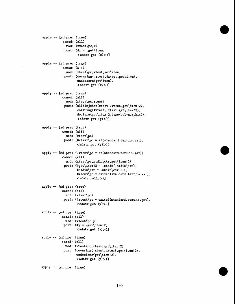
apply ~
apply —
apply
apply —
apply
[sd pre: (true) comod: (all)
mod: (xtest\pc,x) post: (#x = .get\item,
<adatr get (x)>)]
[sd pre: (true) comod: (all)
mod: (xtest\pc,xtest,get\item) post: (covering(.xtest,#xtest,get\item),
undeclare(get\item), <adatr get (x)>)]
[sd pre: (true) comod: (all)
mod: (xtest\pc,xtest) post: (alldisjoint(xtest,.xtest,get\item
covering(#xtest,.xtest,get\item!2), declare(get\item!2,type(polymorphic)), <adatr get (y)>)]
[sd pre: (true) comod: (all)
mod: (xtest\pc) post: (#xtest\pc = at(standard.text_io.get) ,
<adatr get (y)>)]
[sd pre: (.xtest\pc = at (standard.text-io. get)) comod: (all)
mod: (xtest\pc,stdin\ctr,get\item!2) post: (#get\item!2 = .stdin[.stdin\ctrD,
#stdin\ctr = .stdin\ctr + 1, #xtest\pc = exited(standard.text_io.get), <adatr null;>)]
apply — [sd pre: (true) comod: (all)
mod: (xtest\pc) post: (#xtest\pc = exited(standard.textjLo.get) ,
<adatr get (y)>)]
apply
apply ~
apply
[sd pre: (true) comod: (all)
mod: (xtest\pc,y) post: (#y = .get\item!2,
<adatr get (y)>)]
[sd pre: (true) comod: (all)
mod: (xtest\pc,xtest,get\item!2) post: (covering(.xtest,#xtest,get\item!2)
undeclare(get\item!2), <adatr get (y)>)]
[sd pre: (true)
190

comod: (all) mod: (xtest\pc,xtest)
post: (alldisjoint(xtest, .xtest,get\item!3) , covering(#xtest,.xtest,get\item!3), declare(get\item!3.type(polymorphic)), <adatr get (z)>)]
apply — [sd pre: (true) comod: (all) mod: (xtest\pc)
post: (#xtest\pc = at(standard.text_io.get) , <adatr get (z)>)]
apply —
apply
[sd pre: (.xtest\pc = at(standard.textj.o.get)) comod: (all)
mod: (rtest\pc,stdin\ctr,get\item!3) post: (#get\item!3 = .stdin[.stdüi\ctr] ,
#stdin\ctr = .stdin\ctr + 1, #xtest\pc = exited (standard. text_io. get) , <adatr null;>)]
[sd pre: (true) comod: (all)
mod: (xtest\pc) post: (#xtest\pc = exited(standard.text_io.get) ,
<adatr get (z)>)]
apply —
apply
apply
[sd pre: (true) comod: (all)
mod: (xtest\pc,z) post: (#z = .get\item!3,
<adatr get (z)>)]
[sd pre: (true) comod: (all)
mod: (xtest\pc,xtest,get\item!3) post: (covering(.xtest,#xtest,get\item!3)
undeclare(get\item!3), <adatr get (z)>)]
[sd pre: (true) comod: (all)
mod: (xtest\pc,xtest) post: (alldisjoint(xtest,.xtest.a.b),
covering(#xtest,.xtest.a.b), declare(a,type(integer))»declare(b,type(integer)), <adatr exchange (x, ...)>)]
apply — [sd pre: (true) comod: (all)
mod: (xtest\pc,a,b) post: (#a = .x,#b = .y,
<adatr exchange (x, ...)>)]
apply — [sd pre: (true)
191

comod: (all) mod: (xtest\pc)
post: (#xtest\pc = at(xtest.exchange), <adatr exchange (x, )>)]
go — breakpoint reached
<sdvs.l.29> usable
u(l) [sd pre: (true) comod: (all)
mod: (xtest\pc,xtest) post: (alldisj oint (xtest,.xtest,c),covering(#xtest,.xtest,c),
declare(c,type(integer)), <adatr c : integer>)]
No usable quantified formulas.
Symbolic execution is now at precisely the point where steps 1 and 2 of the first call to the exchange procedure have been completed, where the next step would be the instantiation for the declaration of the local variable. Instead, we can invoke the lemma to bypass symbolic execution of the procedure body.
<sdvs.l.29> invokeadalemma Ada lemma name: exchange.lemma
invokeadalemma — [sd pre: (.xtest\pc = at(xtest.exchange)) comod: (all)
mod: (xtest\pc,a,b) post: (#a = .b,#b = .a,
#xtest\pc = exited(xtest.exchange), <adatr return;>)]
<sdvs.l.30> usable
u(l) [sd pre: (true) comod: (all)
mod: (xtest\pc) post: (#xtest\pc = exited(xtest.exchange),
<adatr exchange (x, ...)>)]
No usable quantified formulas.
< sdvs. 1.30 > apply sd/number [highest applicable/once] : < CR>
apply — [sd pre: (true) comod: (all)
mod: (xtest\pc) post: (#xtest\pc = exited(xtest.exchange),
<adatr exchange (x, ...)>)]
192

<sdvs.l.31> usable
u(l) [sd pre: (true) comod: (all)
mod: (xtest\pc,x,y) post: (#x = .a,#y = .b,
<adatr exchange (x, ...)>)]
No usable quantified formulas.
This point immediately follows the completion of step 5. Two more state deltas are applied to complete steps 6 and 7.
<sdvs.l.31> apply sd/number[highest applicable/once]: 2
apply — [sd pre: (true) comod: (all)
mod: (xtest\pc,x,y) post: (#x = .a,#y = .b,
<adatr exchange (x, ...)>)]
apply — [sd pre: (true) comod: (all)
mod: (xtest\pc,xtest,a,b) post: (covering(.xtest,#xtest,a,b),undeclare(a,b),
<adatr exchange (x, ...)>)]
<sdvs.l.33> usable
u(l) [sd pre: (true) comod: (all)
mod: (xtest\pc,xtest) post: (alldisjoint(xtest,.xtest,a!2,b!2),
covering(#xtest,.xtest,a!2,b!2) , declare(a!2.type(integer)),declare(b!2.type(integer)), <adatr exchange (y, ...)>)]
No usable quantified formulas.
This is the beginning of the next Ada statement.
We go on to the point where the lemma can be invoked again, invoke it, and then apply the state deltas to complete the return from the call.
<sdvs.l.33> go until D: #xtest\pc = at (xtest. exchange)
apply — [sd pre: (true) comod: (all)
193

mod: (xtest\pc,xtest) post: (alldisjoint(xtest, .rtest ,a!2,b!2) ,
covering(#xtest,.xtest,a!2,b!2), declare(a!2,type(integer)), declare(b!2,type(integer)), <adatr exchange (y, ...)>)]
apply — [sd pre: (true) comod: (all) mod: (xtest\pc,a!2,b!2)
post: (#a!2 = .y,#b!2 = .z, <adatr exchange (y, )>)]
apply — [sd pre: (true) comod: (all)
mod: (xtest\pc) post: (#xtest\pc = at(xtest.exchange),
<adatr exchange (y, )>)]
go — breakpoint reached
<sdvs. 1.36> invokeadalemma Ada lemma name: exchange.lemma
invokeadalemma — [sd pre: (.xtest\pc = at(xtest.exchange)) comod: (all)
mod: (xtest\pc,a!2,b!2) post: (#a!2 = .b!2,#b!2 = .a!2,
#xtest\pc = exited(xtest.exchange), <adatr return;>)]
<sdvs.l.37> apply sd/nuaber [highest applicable/once] : ,9
apply — [sd pre: (true) comod: (all)
mod: (xtest\pc) post: (#xtest\pc = exited(xtest.exchange),
<adatr exchange (y, ...)>)]
apply [sd pre: (true) comod: (all)
mod: (xtest\pc,y,z) post: (#y = .a!2,#z = .b!2,
<adatr exchange (y, .)»]
apply — [sd pre: (true) comod: (all)
mod: (xtest\pc,xtest,a!2,b!2) post: (covering(.xtest,#xtest,a!2,b!2),undeclare(a!2,b!2),
<adatr exchange (y, )>)]
<sdvs.l.40> usable
u(l) [sd pre: (true)
194

comod: (all) mod: (xtest\pc,xtest)
post: (alldisjoint(xtest,.xtest,put\item) , covering(#xtest,.xtest,put\item), declare(put\item,type(polymorphic)), <adatr put (x)>)]
No usable quantified formulas.
We now simply go on through the rest of the test program.
<sdvs.l.40> go until []: terminated(xtest)
apply — [sd pre: (true) comod: (all)
mod: (xtest\pc,xtest) post: (alldisjoint(xtest, .xtest,put\item),
covering(#xtest,.xtest,put\item), declare(put\item,type(polymorphic)), <adatr put (x)>)]
apply — [sd pre: (true) comod: (all)
mod: (xtest\pc,put\item) post: (#put\item = .x,
<adatr put (x)>)]
apply — [sd pre: (true) comod: (all)
mod: (xtest\pc) post: (#xtest\pc = at(standard.texxjio.put),
<adatr put (x)>)]
apply — [sd pre: (.xtest\pc = at(standard.text_io.put)) comod: (all)
mod: (xtest\pc,stdout[.stdout\ctr],stdout\ctr) post: (#stdout[.stdout\ctr] = .put\item,
#stdout\ctr = .stdout\ctr + 1, #xtest\pc = exited(standard.text_io.put) , <adatr null;>)]
apply — [sd pre: (true) comod: (all)
mod: (xtest\pc) post: (#xtest\pc =
<adatr put exited(standard.textJ.o.put), (x)»]
apply — [sd pre: (true) comod: (all)
mod: (xtest\pc,xtest,put\item) post: (covering(.xtest,#xtest,put\item) ,
undeclare(put\item), <adatr put (x)>)]
195

apply — [sd pre: (true) comod: (all)
mod: (xtest\pc,xtest) post: (alldisjoint(xtest,.xtest ,put\item!2),
covering(#xtest,.xtest,put\item!2), declare(put\item!2,type(polymorphic)), <adatr put (y)>)]
apply — [sd pre: (true) comod: (all)
mod: (xtest\pc,put\item!2) post: (#put\item!2 = .y,
<adatr put (y)>)]
apply — [sd pre: (true) comod: (all)
mod: (xtest\pc) post: (#xtest\pc = at(standard.text_io.put) ,
<adatr put (y)>)]
apply — [sd pre: (.xtest\pc = at(standard.textj.o.put)) comod: (all)
mod: (xtest\pc,stdout[.stdout\ctr],stdout\ctr) post: (#stdout[.stdout\ctr] = .put\item!2,
#stdout\ctr = .stdout\ctr + 1, #xtest\pc = exited(standard.text-io.put), <adatr null;>)]
apply — [sd pre: (true) comod: (all)
mod: (xtest\pc) post: (#xtest\pc = exited(standard.text_io.put) ,
<adatr put (y)>)]
apply —
apply —
[sd pre: (true) comod: (all)
mod: (xtest\pc,xtest,put\item!2) post: (covering(.xtest,«xtest,put\item!2),
undeclare(put\item!2), <adatr put (y)>)]
[sd pre: (true) comod: (all)
mod: (xtest\pc,xtest) post: (alldisjoint(xtest,.xtest,put\item!3),
covering (#xtest,.xtest,put\item!3), declare(put\item!3.type(polymorphic)) , <adatr put (z)>)]
apply [sd pre: comod:
mod: post:
(true) (all) (xtest\pc,put\item!3) (#put\item!3 = .z, <adatr put (z)>)]
196

apply — [sd pre: (true)
comod: (all)
mod: (xtest\pc) post: (#xtest\pc = at (standard.text_io.put) ,
<adatr put (z)>)]
apply — [sd pre: (.xtest\pc = at (standard.text J.o.put))
comod: (all) mod: (rtest\pc,stdout[.stdout\ctr],stdout\ctr)
post: (#stdout[.stdout\ctr] = .put\item!3,
#stdout\ctr = .stdout\ctr + 1,
#xtest\pc = exited (standard. text_io. put) ,
<adatr null;>)]
close — 55 steps/applications
<sdvs.2> ps
<< initial state >> proved xtest.sd <1> —> you axe here <—
The postcondition of xtest.sd is sufficiently simple that the system can verify it without assistance, and the proof closes automatically.
The reader may well wonder why the Ada lemma can be invoked only after a call to the procedure has been partly processed (manually), and why afterwards we still have to apply two more state deltas to complete the call. Why shouldn't the system be programmed to perform these instantiations and state delta applications automatically? In fact, there is no reason why this wouldn't have worked in our example. But here, all the conditions to be proven were simple enough that they could be verified by the simplifier and propagated automatically. With conditions that are more complex, perhaps involving quantifiers, this would not be the case, and the user would need to assist the system in propagating these conditions through the steps at the beginning and end of the procedure call.
4.6 AN EXAMPLE PROOF WITH ADALEMMA
In this final section we give one more example of an SDVS 11 Ada proof for the program packages (Figures 9, 10, and 11).
We create an adalemma and proof as follows:
<sdvs. 2> adatr path name[testproofs/xtest.ada]: testproofs/ada/packages.a
Reading parse tree file for Stage 3 Ada file — "packages.a"
Translating Stage 3 Ada file — "testproofs/ada/packages.a"
<sdvs.3> createadalemma
197

with text_io; use text_io; with integer_io; use integer_io;
procedure packages is
function testl return integer is package p is
x: integer := 10; end p; use p;
begin return x;
end test;
function test2 return boolean is x : boolean := true; package p is
x: integer := 10; end p; use p;
begin return x;
end test;
function test3 return integer is package pi is
x : integer; end pi; package p2 is
x : boolean; end p2; use pi, pi;
begin return x;
end test3;
Figure 9: Program Packages, Part 1
198

function test4 return integer is package pi is
x : integer; end pi; package p2 is
x : boolean; end p2; use pi, p2;
begin return pl.x;
end test4;
procedure test5 is package pO is
v: integer; end pO; package pi is
x: integer; function f return integer; use pO; package p is
z: integer := v; u: integer := x; use pi; package q is
w: integer; end q;
end p; end pi; package p2 is
x: boolean; end p2; use pl.p; use p2; use q;
begin null; « := 2; x := true; z := 1;
end test5;
Figure 10: Program Packages, Part 2
199

procedure exceptions is foo: exception; x: integer; function f (z: integer) return integer is begin raise foo; return 0;
exception when foo => return 1;
end f; package p2 is
x: integer; procedure p(z: integer); package p3 is
x: integer; end p3;
end p2; package body p2 is
w: integer := f(0); procedure p(z: integer) is begin
s := z; put (w) ; raise foo;
end p; begin
x := 5; put(5); raise foo;
exception when foo => x := 23;
put(x); raise;
end p2; begin p2.p(86); exception
when foo => put(lOO); end exceptions;
begin null;
end packages;
Figure 11: Program Packages. Part 3 (conclusion)
200

lemma name: packages.exceptions.lemma file name: testproofs/ada/packages.a
subprogram name: exceptions qualified name: packages.exceptions
preconditions[] : alldisjoint(stdout[l], stdoutß]), .stdout\ctr = 1 mod list [] : all
postconditions: #stdout[l]=5, #stdout[2]=23
createadalemma — [sd pre: (.packages\pc = at (packages, except ions) , alldisjoint (stdout [1] ,stdout [2]) , .stdout\ctr = 1)
comod: (all) mod: (packages\pc,all)
post: («stdout[1] = 5,«stdout[2] = 23, #packages\pc = exited(packages.exceptions))]
<sdvs. 4> proveadalemma Ada lemma name: packages.exceptions.lemma
proof [] : < CR>
open— [sd pre: (alldisjoint(packages,.packages), covering(.packages,packages\pc,stdin,stdin\ctr,stdout,
stdout\ctr), declare(stdout\ctr,type(integer)), declare(stdout »type(polymorphic)), declare(stdin\ctr,type(int eger)), declare(stdin,type(polymorphic)), <adatr exceptions;>)
comod: (all) mod: (all)
post: ([sd pre: (.packages\pc = at(packages.exceptions), alldisjoint (stdout [l'J , stdout [2] ) , .stdout\ctr = 1)
comod: (all) mod: (diff(all,
diff(union(packages\pc,stdin,stdin\ctr, stdout,stdout\ctr),
union(packages\pc,all) ) ) ) post: («stdout[1] = 5,«stdout[2] = 23,
#packages\pc = exited(packages.exceptions))])]
apply — [sd pre: (true) comod: (all)
mod: (packages\pc) post: (#packages\pc = at(packages.exceptions),
<adatr null;>)]
go — breakpoint reached
open — [sd pre: (.packages\pc = at(packages.exceptions), alldisjoint(stdout[l],stdout[2]),.stdout\ctr = 1)
comod: (all) mod: (diff(all,
diff(union(packages\pc,stdin,stdin\ctr.stdout, stdout\ctr),
201

union(packages\pc,all)))) post: (#stdout[l] = 5,#stdout[2] = 23,
#packages\pc = exited(packages.exceptions))]
<sdvs.4.2.1> go until [] : #packages\pc = exited(packages.exceptions)
apply — [sd pre: (true) comod: (all)
mod: (packages\pc,packages) post: (alldisjoint(packages,.packages,exceptions.x),
covering(«packages,.packages,exceptions.x), declare(exceptions.x,type(integer)), <adatr x : integer>)]
apply — [sd pre: (true) comod: (all) mod: (packages\pc,packages)
post: (alldisjoint(packages,.packages,exceptions.p2.x), covering(«packages,.packages,exceptions.p2.x), declare(except ions.p2.x,type(integer)), <adatr x : integer>)]
apply — [sd pre: (true) comod: (all) mod: (packages\pc,packages)
post: (alldisjoint(packages,.packages,p3.x), covering(»packages,.packages,p3.x), declare(p3.x,type(integer)), <adatr x : integer>)]
apply — [sd pre: (true) comod: (all) mod: (packages\pc,packages)
post: (alldisjoint(packages,.packages,exceptions.f ), covering(«packages,.packages,exceptions.1), declare(exceptions.f,type(integer)), <adatr null;>)]
apply — [sd pre: (true) comod: (all)
mod: (packages\pc,packages) post: (alldisjoint(packages,.packages,f.z),
covering(«packages,.packages,f.z), declare(f.z.type(integer)), <adatr f (0)>)]
apply
apply —
[sd pre: (true) comod: (all)
mod: (packages\pc,f.z) post: («f.z = 0,
<adatr f (0)>)]
[sd pre: (true) comod: (all)
202

mod: (packages\pc) post: (#packages\pc = at(packages.exceptions.f),
<adatr f (0)>)]
apply — [sd pre: (true) comod: (all)
mod: (packages\pc,exceptions.f) post: (»exceptions.f = 1,
<adatr return 1;>)]
apply — [sd pre: (true) comod: (all)
mod: (packages\pc) post: (#packages\pc = exited(packages.exceptions.f),
<adatr f (0)>)3
apply — [sd pre: (true) comod: (all)
mod: (packages\pc,packages,f.z) post: (covering(.packages,»packages,f.z),undeclare(f.z),
<adatr i (0)>)]
apply — [sd pre: (true) comod: (all)
mod: (packages\pc,packages) post: (alldisjoint(packages,.packages,p2.w),
covering(»packages,.packages,p2. w), declare(p2.w,type(integer)), <adatr w : integer := f (0)>)]
apply — [sd pre: (true) comod: (all)
mod: (packages\pc,p2.w) post: (#p2.w = .exceptions.!,
<adatr w : integer := f (0)>)]
apply — [sd pre: (true) comod: (all)
mod: (packages\pc,except ions.p2.x) post: (»exceptions.p2.x = 5,
<adatr x := 5;>)]
apply — [sd pre: (true) comod: (all)
mod: (packages\pc,packages) post: (alldisjoint(packages,.packages,put\item),
covering(»packages,.packages,put\item), declare(put\item,type(polymorphic)), <adatr put (5)>)]
apply — [sd pre: (true) comod: (all)
mod: (packages\pc,put\item) post: (»put\item = 5,
<adatr put (5)>)]
203

apply — [sd pre: (true) comod: (all)
mod: (packages\pc) post: (#packages\pc = at (standard, text .io.put) ,
<adatr put (5)>)]
apply — [sd pre: (.packages\pc = at(standard.text_io.put)) comod: (all)
mod: (packages\pc,stdout[.stdout\ctr],stdout\ctr) post: (#stdout[.stdout\ctr] = .put\item,
#stdout\ctr = .stdout\ctr + 1, #packages\pc = exited (standard, text JLO. put) , <adatr null;>)]
apply — [sd pre: (true) comod: (all)
mod: (packages\pc) post: (#packages\pc = exited(standard.text_io.put) ,
<adatr put (5)>)]
apply — [sd pre: (true) comod: (all)
mod: (packages\pc,packages,put\item) post: (covering(.packages,»packages,put\item),
undeclare(put\item), <adatr put (5)>)]
apply — [sd pre: (true) comod: (all)
mod: (packages\pc,except ions.p2.x) post: (»exceptions.p2.x = 23,
<adatr x := 23;>)]
apply — [sd pre: (true) comod: (all)
mod: (packages\pc,packages) post: (alldisjoint(packages,.packages,put\item!2),
covering(«packages,.packages,put\item!2), declare(put\item!2.type(polymorphic)), <adatr put (x)>)]
apply —
apply --
[sd pre: (true) comod: (all)
mod: (packages\pc,put\item!2) post: (#put\item!2 = .exceptions.p2.x,
<adatr put (x)>)]
[sd pre: (true) comod: (all)
mod: (packages\pc) post: (#packages\pc = at(standard.text-io.put),
<adatr put (x)>)]
apply — [sd pre: (.packages\pc = at(standard.text_io.put))
204

comod: (all) mod: (packages\pc,stdout[.stdout\ctr],stdout\ctr) post: (#stdout[.stdout\ctr] = .put\item!2,
#stdout\ctr = .stdout\ctr + 1, #packages\pc = exited(standard.text_io.put) ,
<adatr null;>)]
apply — [sd pre: (true) comod: (all)
mod: (packages\pc) post: (#packages\pc = exited(standard.text_io.put),
<adatr put (x)>)]
[sd pre: (true) comod: (all) mod: (packages\pc,packages,put\item!2)
post: (covering(.packages,»packages,put\item!2),
apply
undeclare(put\item!2), <adatr put (x)>)]
apply — [sd pre: (true) comod: (all)
mod: (packages\pc,packages,p2.w) post: (covering(.packages,»packages,p2.w),
undeclare (p2. n), <adatr w : integer := i (0)>)]
apply — [sd pre: (true) comod: (all) mod: (packages\pc,packages,p3.x) post: (covering(.packages,»packages,p3.x),
undeclare (p3. x) , <adatr x : integer>)]
apply — [sd pre: (true) comod: (all) mod: (packages\pc,packages,except ions.p2.x) post: (covering(.packages,»packages,exceptions.p2.x),
undeclare(except ions.p2.x), <adatr x : integer>)]
apply — [sd pre: (true) comod: (all) mod: (packages\pc,packages,exceptions.x)
post: (covering(.packages,»packages,exceptions.x), undeclare(exceptions.x), <adatr x : integer>)]
apply — [sd pre: (true) comod: (all)
mod: (packages\pc) post: (#packages\pc = exited(packages.exceptions),
<adatr null;>)]
close — 31 steps/applications
205

close — 2 steps/applications
proveadalemma — [sd pre: (.packages\pc = at(packages.exceptions), alldisjoint(stdout[l] ,stdout[2]) , .stdout\ctr = 1)
comod: (all) mod: (packages\pc,all)
post: (#stdout[l] = 5,#stdoirt[2] = 23, #packages\pc = exited(packages.exceptions))]
206

5 INTERACTION WITH VHDL
VHDL (VHSIC Hardware Description Language) is an IEEE standard hardware description language, for which [21] is the definitive reference. SDVS 11 has the capability to translate from a subset of the language — Stage 2 VHDL — into state deltas, and to prove claims about the resulting hardware description representations.
We present a brief description of the Stage 2 VHDL language subset and an example proof of a property of a VHDL hardware description. The Stage 2 VHDL translator itself is documented in detail in [49], on which the next section is based.
Our projections for the partition of VHDL into language subsets are set forth in [26] (the features actually included in the first three subsets have deviated somewhat from this plan). Example correctness proofs for hardware descriptions written in the initial subset, Core VHDL, are discussed in [51]. The translator for the second subset, Stage 1 VHDL, is described in [50]. For further information on the evolution of the state delta semantics for VHDL, refer to [22], [23], [27], and [24].
The command vhdltr operates like adatr, but takes as argument the name of a file containing a VHDL description to be translated.
5.1 INTRODUCTION
Prior to 1987, we adapted SDVS to handle a subset of the hardware description language ISPS. However, ISPS has serious limitations regarding the specification of hardware at levels other than the register transfer level. In 1988 we documented a study of some of the hardware verification research being performed outside Aerospace and investigated VHDL, an IEEE and DoD standard hardware description language released in December 1987. We selected VHDL as a possible medium for hardware description within SDVS.
Prerequisites for adapting SDVS to VHDL are (1) to define VHDL semantics formally in terms of SDVS's underlying logic (the state delta logic) and (2) to implement a translator from VHDL to the state delta logic. As with the incorporation of Ada into SDVS, the approach taken with VHDL has been to implement increasingly complex language subsets; this enables a graded, structured approach to hardware verification.
In 1989 we defined an initial subset of VHDL, called Core VHDL, that captured the essen- tial behavioral features of VHDL. We defined both the concrete syntax and abstract syntax for Core VHDL, formally specified its semantics and, on the basis of this semantic defini- tion, implemented a Core-VHDL-to-state-delta translator. In 1990, SDVS was enhanced to provide the capability of verifying hardware descriptions written in Core VHDL. In 1991 and 1992, the translator underwent extensive revisions to accommodate Stage 1 VHDL and Stage 2 VHDL, respectively.
The VHDL translator essentially functions as a simulator kernel, maintaining a clock and a list of future events that are defined as state deltas. For Core VHDL, however, the translator transformed possibly multiple Core VHDL statements: sequential statements between WAIT
207

Statements within a process were all translated and then composed into a single state delta. The translator updated the clock to the next time at which a signal driver became active or a process resumed. As the clock advanced, the translator merged the composite state deltas into a single state delta that specified the behavior of all processes at that point in the execution.
For Stage 1 VHDL, we reevaluated the feasibility of using composition in the translation of VHDL to state deltas, and concluded that although composition had initially seemed viable in the case of Core VHDL, it is impossible in principle to apply the technique to more complex VHDL subsets, as the attempt would require the ability to compose over sections of VHDL code that would necessitate static proof in SDVS. More generally, the ability to compose over arbitrary WAIT-bracketed code in PROCESS statements would be tantamount to the automatic construction of correctness proofs without user intervention — a theoretically undecidable problem.
Therefore, we decided to abandon composition for Stage 1 VHDL and succeeding SDVS VHDL subsets. Instead, within a given execution (simulation) cycle, processes are translated sequentially, in the order in which they appear in the VHDL description, and the user has control over stepping through the sequential statements within each process. Thus, rather than trying to have the VHDL translator model the concurrency of the processes, we chose to take for granted a certain "metatheorem" about VHDL: that any two sequentializations of the processes are equivalent. A brief justification for this point of view is that the problem of mutual exclusion is not a concern in VHDL, since
• all variables are local to the process in which they are declared, and
• distinct processes modify distinct drivers of a given signal (known as a resolved signal), and the ultimate signal value is obtained by the application of a user-defined resolution function.9
A gratifying benefit of the revised translation strategy is that the understandability of the resulting proofs has been remarkably improved — the dynamic flow of process execution precisely reflects the simulation semantics of VHDL (as defined in the VHDL Language Reference Manual [21]), but with the crucial aspect of symbolic execution (the use of ab- stract values rather than concrete) thrown in. The current VHDL translator thus functions as a "symbolic simulator," and is a considerably more intuitive proof engine than was its incarnation for Core VHDL.
5.2 STAGE 2 VHDL
Stage 2 VHDL comprises a relatively powerful behavioral subset of VHDL. That is to say, Stage 2 VHDL descriptions are confined to the specification of hardware behavior or data flow, rather than structure. More comprehensive VHDL subsets for SDVS (anticipated: Stage 3 VHDL) will include constructs for the structural description of hardware in terms
9 As of Stage 2 VHDL, however, resolved signals are still disallowed.
208

of its hierarchical decomposition into connected subcomponents. The Stage 2 VHDL data types are: BOOLEAN, BIT, INTEGER, REAL (preliminary version), TIME (a predefined physical type of INTEGER range), CHARACTER, STRING (arrays of characters), BIT_VECTOR (arrays of bits), user-defined enumeration types, and user-defined array types.
The primary VHDL abstraction for modeling a digital device is the design entity. A design entity consists of two parts: an entity declaration, providing an external view of the compo- nent by declaring the input and output ports, and an architecture body, giving an internal view in terms of component behavior or structure.
In Stage 2 VHDL, each architecture body is constrained to be behavioral, consisting of a set of declarations and concurrent statements defining the functional interpretation of the device being modeled. The allowable concurrent statements are of two kinds: PROCESS statements and concurrent signal assignment statements, to be discussed below.
A PROCESS statement, the most fundamental kind of behavioral concurrent statement in VHDL, is a block of sequential zero-time statements that execute sequentially but "in- stantaneously" in zero time [27], and some (possibly none) distinguished sequential WAIT statements whose purpose is to suspend process execution and allow time to elapse.
A process typically schedules future values to appear on data holders called signals, by means of sequential signal assignment statements. The execution of a signal assignment statement does not immediately update the value of the target signal (the signal assigned to); rather, it updates the driver associated with the signal by placing (at least one) new transaction, or time-value pair, on the waveform which is the list of such transactions contained in the driver. Each transaction projects that the signal will assume the indicated value at the indicated time; the time is computed as the sum of the current clock time of the model and the delay specified (explicitly or implicitly) by the signal assignment statement.
Two types of time delay can be specified by a sequential signal assignment statement, and Stage 2 VHDL encompasses both. Inertial delay, the default, models a target signal's inertia that must be overcome in order for the signal to change value; that is, the scheduled new value must persist for at least the time period specified by the delay in order actually to be attained by the target signal. Transport delay, on the other hand, must be explicitly indicated in the signal assignment statement with the reserved word TRANSPORT, and models a "wire delay" wherein any pulse of whatever duration is propagated to the target signal after the specified delay.
In lieu of explicit WAITs, a process may have a sensitivity list of signals that activate process resumption upon receiving a distinct new value (an event). The sensitivity fist implicitly inserts a WAIT statement as the last statement of the process body.
The other class of concurrent statement in Stage 2 VHDL is that of concurrent signal assignment statements. These always represent equivalent PROCESS statements, and come in two varieties: conditional signal assignment and selected signal assignment. A conditional signal assignment is equivalent to a process with an embedded IF statement whose branches are sequential signal assignments; similarly, a selected signal assignment is equivalent to a process with an embedded (possibly degenerate) CASE statement whose branches are
209

sequential signal assignments. The VHDL translator syntactically transforms concurrent signal assignment statements to their corresponding PROCESS statements before translating them into state deltas.
Signals act as data pathways between processes. Each process applies operations to values being passed through the design entity. We may regard a process as a program implementing an algorithm, and a Stage 2 VHDL description as a collection of independent programs running in parallel.
In full VHDL, a target signal can be assigned to in multiple processes, in which case it possesses correspondingly many drivers for updating by the different processes; the value taken on by the signal at any particular time is then computed by a user-defined resolution function of these drivers. As did previous SDVS VHDL subsets, Stage 2 VHDL disallows such resolved signals: a signal is not permitted to appear as the target of a sequential signal assignment statement in more than one process body; equivalently, every signal has a unique driver.
Concrete and abstract syntaxes for Stage 2 VHDL have been denned [49] — as required, of course, for the implementation of the Stage 2 VHDL translator. Perhaps the following summary provides the best way of seeing the Stage 2 VHDL language subset and translator at a glance.
• VHDL design files
— user-defined packages (optional), USE clauses (optional), entity declaration, ar- chitecture body
— restriction: unique entity and architecture per file
• package STANDARD
— predefined types: BOOLEAN, BIT, INTEGER, TIME, CHARACTER, REAL, STRING, BIT.VECTOR
— various units of type TIME: FS, PS, NS. US, MS, SEC, MIN. HR
— restriction: implementation of type REAL is preliminary; supports parsing and Phase 1 translation but no Phase 2 reasoning
• user-defined packages
— package declarations
— package bodies
• USE clauses for accessing packages
• entity declarations
— entity header: port declarations
— entity declarative part: other declarations
• architecture bodies
210

• object declarations
- CONSTANT, VARIABLE, SIGNAL
- octal and hexadecimal representations of bitstrings
- entity ports of default object class SIGNAL
• array type declarations
- arrays (bidirectional; constrained or not) of. arbitrary element type
- attributes 'low and 'high for lower and upper bounds of an array type (restric- tion: but not of an array object)
• user-defined enumeration types
• signals of arbitrary array and enumeration types
• subprograms
- procedures and functions: declarations and bodies
- restriction: excluding parameters of object class SIGNAL
• concurrent statements
- PROCESS statements
- conditional signal assignments
- selected signal assignments
• sequential statements
- null statement: NULL
- variable assignments (scalar k. composite)
- signal assignments (scalar & composite, inertial or TRANSPORT delay)
- conditionals: IF, CASE
- loops: LOOP, WHILE, FOR
- loop exits: EXIT
- subprogram calls
- subprogram return: RETURN
- process suspension: WAIT
• operators
- numeric unary operators: ABS, +, -
- numeric binary operators: +, -, *, /, ** (exponentiation), HOD (modulus), REM (remainder)
- boolean and bit operators: NOT, AND, NAND, OR, NOR, XOR
211
— relational operators: =, /=, <, <=, >, and >=
— array concatenation operator: &
— restriction: =, /=, and & are the only Stage 2 VHDL operators defined for user- defined array types
5.3 TRANSLATION OF STAGE 2 VHDL
A Stage 2 VHDL hardware description is first parsed according to the Stage 2 VHDL grammar, producing an abstract syntax tree that serves as the input to Phase 1 of the translation.
Phase 1 of the translation accomplishes the following.
• Performs static semantic checks to verify that certain conditions are met, for example:
Objects, subprograms, packages, and process and loop labels must be declared prior to use.
Identifiers with the same name cannot be declared in the same local context.
References to objects and labels must be proper, e.g. scalar objects must not be indexed, array references must have the correct number of indices, and EXIT state- ments must reference a loop label.
All components of statements and expressions must have the proper type, e.g. expressions used as conditions must be boolean, array indices must be of the proper type, operators must receive operands of the correct type, procedure and function calls must receive actual parameters of the proper type, function calls must return a result of a type appropriate for their use in an expression.
Sensitivity lists in PROCESS and WAIT statements must contain signal identifiers.
The collection of discrete ranges defining a CASE statement alternative must be exhaustive and mutually exclusive.
The time delays in the AFTER clause of a signal assignment statement must be increasing.
• Creates a new abstract syntax tree — a transformed version of the original abstract syntax tree (used by Phase 1) — that will be more conveniently utilized by Phase 2 of the translation.
• Creates and manipulates a tree-struciured environment (TSE) that, in the absence of errors, is provided to Phase 2 of the translation.
If the VHDL translator completes Phase 1 without error, then it can proceed with Phase 2, state delta generation. Phase 2 requires two inputs: the transformed abstract syntax tree and the tree-structured environment (TSE) for the hardware description, both constructed by Phase 1.
212

The TSE contains a complete record of the name/attribute associations corresponding to the hardware description's declarations, and its structure reflects that of the description. Referring to the TSE, Phase 2 incrementally generates and (per user proof commands) applies state deltas via symbolic execution and the theories built into the Simphfier.
To understand Phase 2 of the VHDL translator, it is important to recognize that in defin- ing the semantics of concurrent processes within a given architecture body, the translator involves a significant operational component. This is to be distinguished from the seman- tics of sequential statements within processes, which the translator defines in a primarily
denotational manner.
We are referring here to our strategy of designing aspects of a simulator kernel into the VHDL translator. After the application of the state deltas specifying the behavior of one execution cycle for the active processes, the translator is responsible for
• determining the next VHDL clock time at which a driver becomes active or a process
resumes,
• advancing the SDVS state to this new time, and
• generating the state delta that specifies the next sequential statement in the first resuming process for the new execution cycle.
After a given resuming process suspends, its continuation is the textually next resuming process, or "end of execution cycle" when none such remain. The internal translator machin- ery to perform these tasks is operationally defined, much of it embodied in the translator's implementation rather than described by semantic equations.
5.4 AN EXAMPLE
Here we present a very simple example, illustrating the translation of a Stage 2 VHDL hardware description and the manner in which SDVS keeps track of signals and the clock during symbolic execution. The example is a version of one appearing in [51], but modified somewhat to reflect a few of the new language features available in Stage 2 VHDL.
213

— /U/VERSYS/SDVS/TESTPR00FS/VHDL2/SWITCH.VHDL
DESIGNJTLE switch IS
PACKAGE switch4>ackage IS
CONSTANT half^delay : TIME := 500 FS;
END switch-package;
USE switch-package.ALL;
ENTITY switch IS
PORT ( x, y : INOUT INTEGER );
END switch;
ARCHITECTURE behavior OF switch IS
BEGIN
x_gets_y :
x <= y AFTER (2 * half .delay);
y-gets_r :
y <= x AFTER (2 * half ^delay) ;
END behavior;
The Stage 2 VHDL hardware description in file switch.vhdl begins with a line that repre- sents our device for giving a name to the whole description; the tag DESIGN_FILE is not part of official VHDL syntax. This device will disappear once the VHDL design library facility is incorporated into SDVS.
The first interesting section of code is the package declaration of switch-package, which it- self declares the constant half .delay of type TIME (predefined as part of package STANDARD) that will be referenced in the architecture body. The TIME unit FS represents femtoseconds (1 femtosecond = 10-15 second).
214

The USE clause is necessary to make the declaration(s) in switch-package accessible to the
rest of the description.
The entity declaration, or interface, of the description declares two ports x and y; these are signals connecting the hardware device being modeled to other (unspecified) devices in the design environment. The ports are of mode inout, meaning that they may be both read from and written to by the accompanying architecture body.
The architecture body consists of two labeled concurrent signal assignment statements (de- generate selected signal assignments, actually), each of which schedules the current value of a "source" port to become the future value of the other "target" port after 1000 femtosec- onds, or 1 picosecond.
As indicated in Section 5.2, each of the concurrent signal assignments is equivalent to a process that (1) has a similar, but unlabeled, sequential signal assignment statement as its body, and (2) waits for an event — an actual change in the value of the source port — in order to resume execution. We simply continue to refer to these processes in the sequel.
The net effect is to describe a device that switches the values of x and y every picosecond, provided their original values are different, and only a single time provided their original values are the same.
We wish to formulate and prove the following claim about the VHDL description switch:
At any time at which the translation of switch.vhdl holds, there will be a time when the declarations of switch.vhdl have been elaborated, and such that (1) if the input values of x and y are the same, then they will be switched 1 picosecond later and the VHDL model will have completed execution, whereas (2) if the input values are different, the values of x and y will be switched 1 picosecond later, and then in 1 more picosecond they will be switched again.
This English-language specification is formulated as the state delta switch2.sd, which we
read from a file:
<sdvs.l> read path name[testproofs/foo.proofs]: testproofs/vhdl2/switch.spec
Definitions read from file "testproofs/vhdl2/switch.spec" — (switchl.sd,switch2.sd,switch2.badsd,switch2.sd2)
<sdvs.2> ppsd state delta: switchS.sd
[sd pre: (vhdl(switch.vhdl)) mod: (all)
post: (vhdl-modeljelaboratioiucomplete(switch) , [sd pre: (.x = .y)
comod: (all) mod: (all)
post: (»vhdltime = vhdltime(1000,0),#x = .y,#y = .x,
215

vhdl_model_executionjComplete(switch) )] , [sd pre: Cx "= .y) comod: (all)
mod: (all) post: («vhdltime = vhdltime(1000,0),#x = .y,#y = .
[sd pre: (true) comod: (all) mod: (all)
post: (»vhdltime = vhdltime(2000,0),#x = #y = .i)]>3)]
x,
Our first essential order of business is to translate the VHDL description in switch.vhdl into its state delta representation, vhdl (switch, vhdl), so that we may prove our claim about it. This is done by invoking the VHDL translator with the command vhdltr, giving it the source VHDL file as its argument.
<sdvs.2> vhdltr path name [testproofs/vhdl2/f oo. vhdl] : testproofs/vhdl2/'switch.vhdl
Parsing Stage 2 VHDL file — "testproofs/vhdl2/switch.vhdl"
Translating Stage 2 VHDL file — "testproofs/vhdl2/switch.vhdl"
<sdvs.3> pp object: vhdl file name [switch, vhdl] : switch.vhdl
alldisjoint (switch,.switch) covering (. switch, switch\pc, vhdltime, vhdltime-previous) declare(vhdltime»type(vhdltime)) declare (vhdltime_previous, type (vhdltime) ) .vhdltime = vhdltime(0,0) .vhdltimejprevious = vhdltime(O.O) [sd pre: (true)
comod: (all) mod: (switch\pc)
post: (<VHDLTR>)]
We have just exhibited the "initial segment" of the translation of the switch description, consisting of the declaration and initialization of the places vhdltime and vhdltime_previous, as well as a state delta whose postcondition contains a representation of (a state delta for) the incremental continuation of the translation.
In general, each state delta generated by the VHDL translator will contain, as part of its postcondition, a continuation label enclosed in angle brackets; this continuation label simply stands for the next state delta to be incrementally generated by the translator — the continuation. The generic label <VHDLTR> appears most frequently, but occasionally labels attempt to be more descriptive of the next increment of translation.
Sometimes, as in the initial segment of translation, the translator generates a state delta with precondition (true), comodlist (all), a (\pc) modlist, and only a continuation in
216

the postcondition. Such a state delta corresponds to an action, to be unconditionally performed by the translator, resulting in no change in the state (contents of places) except for the program counter. When such a state delta is applied, for brevity it is not printed out in its entirety in the proof trace; rather, the tag action is printed, followed by the continuation label.
<sdvs.3> setflag flag variable: autoclose on or off[off]: off
setflag autoclose — off
The autoclose flag has been turned off to allow the proof to be developed without SDVS closing it automatically.
We now open the proof of switch2. sd:
<sdvs.4> prove state deltaQ: switchZ.so proof [] : < CR>
open — [sd pre: (vhdl(switch.vhdl)) mod: (all)
post: (vhdljuodeljelaboration-jcomplete (switch) , [sd pre: (.x = .y)
comod: (all) mod: (all)
post: («vhdltime = vhdltime(1000,0),#x = .y, #y = .x, vhdl-model_execution_complete(switch))] ,
[sd pre: (.x "= .y) comod: (all)
mod: (all) post: (#vhdltime = vhdltime(1000,0) ,#x = .y,
#y = .x, [sd pre: (true)
comod: (all) mod: (all)
post: (Jtvhdltime = vhdltime(2000,0) , #x = .y,#y = .x)])])]
Complete the proof.
The automatic elaboration of the VHDL description is accomplished by issuing the SDVS command go with the predicate vhdl_model_elaboration_complete(switch) as the until argument. This elaborates the declarations of the constant half-delay and the entity ports x and y, applying state deltas until the elaboration is complete. Any declarations internal to the architecture body or the processes are also elaborated (in the present example, there are none).
217

<sdvs.4.1> go until[] : vhdLmodeLelaboration.complete(switch)
action — <VHDLTR>
apply — [sd pre: (true) comod: (all)
mod: (switch\pc,switch) post: (alldisjoint(switch,.switch,half jdelay) ,
covering(#switch, .switch, half -delay) , declare(half jdelay,type (integer)) , <VHDLTR»]
apply — [sd pre: (true) comod: (all)
mod: (switch\pc, half jdelay) post: (»halfjdelay = 500,
<VHDLTR>)]
apply — [sd pre: (true) comod: (all)
mod: (switch\pc,switch) post: (alldisjoint(switch,.switch,x,y,driver\x,driver\y),
covering(»switch,.switch,x,y,driver\x,driver\y), declare(x,type(integer)), declare(driver\x,type(waveform,type(integer))), declare(x,type(fn,val(.driver\x,.vhdltime))), declare(y,type(integer)), declare(driver\y,type(waveform,type(integer))), declare(y,type(fn,val(.driver\y,.vhdltime))), <VHDLTR>)]
apply — [sd pre: (true) comod: (all)
mod: (switch\pc,x,y,driver\x,driver\y) post: (#driver\x
= waveform(x,transaction(vhdltime(0,0),x\20)), #driver\y
= waveform(y,transaction(vhdltime(0,0),y\22)), <VHDLTR»]
action — <ELAB0RATE PROCESS: X_GETS_Y>
action ~ <ELAB0RATE PROCESS: Y_GETS_X>
go — breakpoint reached
The evaluation of the three SDVS commands vhdltime, vhdl- signals, and vhdl-processes is a convenient means of querying SDVS about aspects of the state of the Stage 2 VHDL proof. Particularly in the case of signals, this query method provides information in a much more intelligible form than that returned by, say, the query command ppl .
<sdvs.4.8> vhdltime
218

global time = 0
delta time = 0
<sdvs. 4. 8> vhdl-signals signal-names [all] : < CR>
simplify? [no] : <CR>
signal X :
current value = x\20
previous value = x\20
projected output waveform = 0
driver history = (transaction(vhdltime(0,0),x\20))
signal Y :
current value = y\22
previous value = y\22
projected output waveform = 0
driver history = (transaction(vhdltime(0,0),y\22))
The declarations have been symbolically elaborated. For example, places x and driver\x have been created to represent the signal (of the same name) and its driver, respectively, and the contents of driver\x have been initialized with wavef orm(x,transaction(vhdltime(0,0) ,x\20)), a waveform (indexed by x) consisting of a single transaction. This transaction stipulates that at vhdltime(0,0), x acquires the symbolic bit value x\20.
In the display generated by the command vhdl-signals, the driver is split conceptually into two disjoint parts, each represented as a list:
• A projected output waveform, consisting of future transactions scheduled to occur on the signal (some of which might be preempted, or deleted from the waveform, during subsequent execution of the description). The time components of projected transactions are all greater than the placevalue . vhdltime. For ease of reference, the projected transactions are displayed in chronological order according to their time components, so that the next scheduled transaction occurs first in the list.
• A driver history, consisting of those transactions that have already been "actualized," i.e., whose time component is at most the placevalue .vhdltime. For ease of refer- ence once again, but in contradistinction to the projected output waveform, these
219

transactions are displayed in reverse chronological order: the most recent actualized transaction for the signal appears at the head of the driver history, and its value component is always the current value of the signal driver.
Thus, the entire signal driver itself is the concatenation of the reverse of the driver history with the projected output waveform.
<sdvs.4.8> vhdl-processes process-names [all] : <CR>
process X.GETS.Y :
current state = SUSPENDED
scheduled time = VHDLTTME(0,0)
scheduled reason = INITIALIZATION
process Y.GETSJC :
current state = SUSPENDED
scheduled time = VHDLTIME(0,0)
scheduled reason = INITIALIZATION
All processes are shown as currently suspended, because we have not yet begun executing the model, but they are scheduled to "resume" execution at vhdltime(0,0), by reason of the initialization phase of the simulation semantics informally defined in the VHDL LRM [21]. In the initialization phase, each process is executed until it suspends. As the next applicable state delta indicates, the translation is ready to commence model execution.
<sdvs.4.8> nsd
[sd pre: (true) comod: (all)
mod: (switch\pc) post: (<BEGIN VHDL MODEL EXECUTIONS]
<sdvs.4.8> whynotgoal simplify? [no] : < CR>
g(2) [sd pre: (.x = .y) comod: (all)
mod: (all) post: (#vhdltime = vhdltime(1000,0),#x = .y,#y = .x,
vhdl-model-erecutioiLxomplete (snitch) ) ] g(3) [sd pre: (.x ~= .y)
220

comod: (all) mod: (all)
post: («vhdltime = vhdltime(1000,0),#x = .y,#y = .x, [sd pre: (true)
comod: (all) mod: (all)
post: (»vhdltime = vhdltime(2000,0),#x = .y,#y = .x)])]
This is an appropriate point at which to open a proof of the goal g(2). Later, after this goal has been proved, we will also need to prove the goal g(3).
<sdvs.4.8> prove state delta[]: g
number: 2 proof []: <CR>
open — [sd pre: (.x = .y) comod: (all)
mod: (all) post: («vhdltime = vhdltime(1000,0),#x = .y,#y = .x,
vhdl-model jexecut iomcomplet e (swit ch) ) ]
Complete the proof.
<sdvs.4.8.1> go until [] : vhdLmodeLexecutionjComplete(switch)
action — <BEGIN VHDL MODEL EXECOTI0N>
action ~ <BEGIN INITIALIZATION PHASE>
action — <. . . INITIALIZATION PHASE: EACH PROCESS EXECUTES UNTIL SUSPENSI0N>
action — <EXECUTE PROCESS: X_GETS_Y>
apply — [sd pre: (~(preemption(.driver\x, transact ion(t imeplus(.vhdlt ime,
vhdltime(2 * .half .delay,
0)),
•y)))) comod: (all)
mod: (snitch\pc,driver\x) post: (#driver\x
= inert iaLjipdat e (. driver\x, transact ion(t imeplus(.vhdlt ime,
vhdltime(2 * .half jdelay,
0)), • y)),
<VHDLTR>)]
action — <SUSPEND PROCESS: X_GETS_Y>
221

action — <... INITIALIZATION PHASE: EACH PROCESS EXECUTES UNTIL SUSPENSION>
action -- <EXECUTE PROCESS: Y.GETSJO
apply — [sdpre: (~(preemption(.driver\y, transact ion(t imeplus(.vhdlt ime,
vhdltime(2 * .half .delay,
0)), .x))))
comod: (all) mod: (switch\pc,driver\y)
post: (#driver\y = inertialjupdate(.driver\y,
transact ion(t imeplus(.vhdlt ime, vhdltime(2 *
.halfjdelay, 0)),
• x))(
<VHDLTR>)]
action — <SUSPEND PROCESS: Y.GETSJO
action — <END INITIALIZATION PHASE>
action -- <BEGIN EXECUTION CYCLE: 1. ADVANCE EXECUTION TIME, 2. UPDATE SIGNALS, 3. RESUME PR0CESSES>
apply — [sd pre: (true) comod: (all) mod: (switch\pc,vhdltime,vhdltime_previous,x,y)
post: (tvhdltime = vhdltime(lOOO.O), #vhdltime_previous = .vhdlt ime, <UPDATE SIGNALS>)]
action ~ <RESUME (?) NEXT SCHEDULED PROCESS: X.GETS_Y>
apply — [sd pre: (.y = val(.driver\y, .vhdltime.previous)) comod: (all) mod: (switch\pc)
post: «RESUME (?) NEXT SCHEDULED PROCESS: Y.GETSJO)]
apply — [sd pre: (.x = val(.driver\x, .vhdltime-previous)) comod: (all) mod: (switch\pc)
post: (<END EXECUTION CYCLE>)]
action — <BEGIN EXECUTION CYCLE: 1. ADVANCE EXECUTION TIME, 2. UPDATE SIGNALS, 3. RESUME PROCESSES>
action — <END VHDL MODEL EXECUTI0N>
222

apply — [sd pre: (true) comod: (all)
mod: (switch\pc) post: (vhdljnodel_execution_complete(switch))]
go — breakpoint reached
<sdvs.4.8.20> vhdltime
global time = 1000
delta time = 0
<sdvs.4.8.20> vhdi-signals signal-names [all] : < CR>
simplify? [no] : yes
signal X :
current value = y\22
previous value = y\22
projected output waveform = 0
driver history = (transaction(vhdltLme(2 * 500,0),y\22).transaction(vhdltime(0,0),y\22))
signal Y :
current value = y\22
previous value = y\22
projected output waveform = ()
driver history = (transaction(vhdltime(2 * 500,0),y\22),transaction(vhdltime(0,0),y\22))
<sdvs.4.8.20> goals
g(l) #vhdltime = vhdltime(1000,0)
g(2) #x = y\29
g(3) #y = x\28 g(4) vhdl-modeljexecution_complete (switch)
<sdvs.4.8.20> whynotgoal simplify? [no] : < CR>
The goal is TRUE. Type 'close'.
223

<sdvs.4.8.20> close
close — 19 steps/applications
Complete the proof.
<sdvs.4.9> goals
g(l) vhdl-model_elaborationjcomplete (switch) g(2) true g(3) [sd pre: (.x "= .y)
comod: (all) mod: (all)
post: (»vhdltime = vhdltime(1000,0),#x = -y,#y = .x, [sd pre: (true)
comod: (all) mod: (all)
post: (»vhdltime = vhdltime(2000,0),#x = .y,#y = .x)])]
<sdvs. 4. 9> whynotgoal simplify? [no] : < CR>
g(3) [sd pre: (.x "= .y) comod: (all)
mod: (all) post: (#vhdltime = vhdltime(1000,0),#x = -y,#y = .x,
[sd pre: (true) comod: (all)
mod: (all) post: (»vhdltime = vhdltime(2000,0),#x = .y,#y = .x)])]
<sdvs.4.9> prove state delta[] : g
number: 3 proof []: <CR>
open — [sd pre: (.x "= .y) comod: (all)
mod: (all) post: (»vhdltime = vhdltime(1000,0),#x = .y,#y = .x,
[sd pre: (true) comod: (all)
mod: (all) post: (»vhdltime = vhdltime(2000,0),#x = .y,
*y = -x)])]
Complete the proof.
<sdvs.4.9.1> go until [] : #vhdltime = vhdltime(1000,0)
action — <BEGIN VHDL MODEL EXECUTI0N>
action — <BEGIN INITIALIZATION PHASE>
224

action — <... INITIALIZATION PHASE: EACH PROCESS EXECUTES UNTIL SUSPENSION>
action — <EXECUTE PROCESS: X_GETS.Y>
apply — [sd pre: (~(preemption(.driver\x, transaction(timeplus(. vhdltime,
vhdltime(2 * .halfjielay,
0)), •y))))
comod: (all) mod: (switch\pc,driver\x)
post: (#driver\x = inert ialJipdate (. driver\x,
transaction(timeplus(.vhdltime, vhdltime(2 *
.halfjielay, 0)),
• y)), <VHDLTR»]
action — <SUSPEND PROCESS: X_GETS_Y>
action — <... INITIALIZATION PHASE: EACH PROCESS EXECUTES UNTIL SUSPENSION>
action — <EXECUTE PROCESS: Y_GETS_X>
apply — [sd pre: (~(preemption(.driver\y, transaction(timeplus(.vhdltime,
vhdltime(2 * .halfjielay,
0)), .x))))
comod: (all) mod: (switch\pc,driver\y)
post: (#driver\y = inertialjapdate (.driver\y,
transaction(timeplus(.vhdltime, vhdltime(2 *
.halfjielay, 0)),
.x)), <VHDLTR>)]
action ~ <SUSPEND PROCESS: Y_GETS-X>
action — <END INITIALIZATION PHASE>
action — <BEGIN EXECUTION CYCLE: 1. ADVANCE EXECUTION TIME,
2. UPDATE SIGNALS, 3. RESUME PROCESSES>
apply — [sd pre: (true) comod: (all)
225

mod: (switch\pc,vhdltime,vhdltime_previous,x,y) post: («vhdltime = vhdltime(1000,0),
#vhdltime_previous = .vhdltime, <UPDATE SIGNALS>)]
go — breakpoint reached
<sdvs.4.9.14> vhdltime
global time = 1000
delta time = 0
<sdvs.4.9.14> vhdl-signah signal-names [all] : <CR>
simplify? [no] : yes
signal X :
current value = y\22
previous value = x\20
projected output waveform = ()
driver history = (transaction(vhdltime(1000,0),y\22),transaction(vhdltime(0,0),x\20))
signal Y :
current value = x\20
previous value = y\22
projected output waveform = ()
driver history = (transaction(vhdltime(1000,0),x\20),transaction(vhdltime(0,0),y\22))
<sdvs.4.9.14> goals
g(l) «vhdltime = vhdltime(1000,0) g(2) #x = y\60 g(3) #y = x\59 g(4) [sd pre: (true)
comod: (all) mod: (all)
post: (»vhdltime = vhdltime(2000,0),#x = .y,#y = .x)]
<sdvs.4.9.14> whynotgoal simplify?[no] : <CR>
226

g(4) [sd pre: (true) comod: (all)
mod: (all) post: («vhdltime = vhdltime(2000,0) ,#x = .y,#y = .x)]
<sdvs.4.9.14> prove state delta[] : g
number: 4 proof []: <CR>
open — [sd pre: (true) comod: (all)
mod: (all) post: (#vhdltime = vhdltime(2000,0),#x = .y,#y = .x)]
Complete the proof.
<sdvs.4.9.14.1> go untilD : #vhdltime = vhdltime(2000,0)
action — <RESUME (?) NEXT SCHEDULED PROCESS: X_GETS_Y>
apply — [sd pre: (.y ~= val(.driver\y, .vhdltime-previous)) comod: (all)
mod: (ssitch\pc) post: ([sd pre: (true)
comod: (all) mod: (switch\pc)
post: «EXECUTE PROCESS: X.GETS_Y>)])]
action — <EXECUTE PROCESS: X_GETS_Y>
apply — [sd pre: (~(preemption(.driver\x, transaction(timeplus(.vhdltime,
vhdltime(2 * .half .delay,
0)), •y))))
comod: (all) mod: (switch\pc,driver\x)
post: (#driver\x = inert ial jipdat e (. dr iver\x,
transaction(timeplus(.vhdlt ime, vhdltime(2 *
.half -delay, 0)),
• y)), <VHDLTR>)]
action — <SUSPEND PROCESS: X.GETS_Y>
action — <RESUME (?) NEXT SCHEDULED PROCESS: Y-GETS_X>
apply — [sd pre: (.x "= val(.driver\x, .vhdltime-previous)) comod: (all)
227

mod: (switch\pc) post: ([sd pre: (true)
comod: (all) mod: (sHitch\pc)
post: (<EXECUTE PROCESS: Y.GETSJC»])]
action — <EXECUTE PROCESS: Y.GETSJO
apply — [sd pre: (~(preemption(.driver\y, transaction(timeplus(.vhdltime,
vhdltime(2 * .half-delay,
0)), •x))))
comod: (all) mod: (switch\pc,driver\y)
post: (#driver\y = inert ial jupdat e (. dr iver\y,
transaction(timeplus(.vhdltime, vhdltime(2 *
.half .delay, 0)),
.i)), <VHDLTR»]
action — <SUSPEND PROCESS: Y.GETSJO
action — <END EXECUTION CYCLE>
action ~ <BEGIN EXECUTION CYCLE: 1. ADVANCE EXECUTION TIME, 2. UPDATE SIGNALS, 3. RESUME PR0CESSES>
apply — [sd pre: (true) comod: (all)
mod: (switch\pc,vhdltime,vhdlxime.previous,x,y) post: («vhdltime = vhdltime(2000,0),
#vhdltime.previous = .vhdltime, <UPDATE SIGNALS»]
go — breakpoint reached
<sdvs.4.9.14.14> vhdltime
global time = 2000
delta time = 0
<sdvs.4.9.14.14> vhdl-signals signal-names [all] : <CR>
simplify?[no] : yes
228

signal X :
current value = x\20
previous value = y\22
projected output waveform = 0
driver history = (transaction(vhdltime(2000,0),x\20),transaction(vhdltime(1000,0),y\22),
transaction(vhdltime(0,0),x\20))
signal Y :
current value = y\22
previous value = x\20
projected output waveform = 0
driver history = (transaction(vhdltime(2000,0),y\22),transaction(vhdltime(1000,0),x\20), transaction(vhdltime(0,0),y\22))
<sdvs.4.9.14.14> goals
g(l) »vhdltime = vhdltime(2000,0) g(2) #x = y\78 g(3) #y = x\79
<sdvs.4.9.14.14> whynotgoal simplify? [no] : < CR>
The goal is TRUE. Type 'close'.
<sdvs.4.9.14.14> close
close — 13 steps/applications
Complete the proof.
<sdvs.4.9.15> goals
g(l) «vhdltime = vhdltime(1000,0) g(2) #x = y\60 g(3) #y = x\59 g(4) true
<sdvs.4.9.15> whynotgoal simplify? [no] : < CR>
The goal is TRUE. Type 'close'.
<sdvs.4.9.15> close
229

close — 14 steps/applications
Complete the proof.
<sdvs.4.10> goals
g(l) vhdljaodel_elaboration_complete(switch) g(2) true g(3) true
<sdvs.4.10> whynotgoal simplify? [no] : < CR>
The goal is TRUE. Type 'close'.
<sdvs.4.10> close
close — 9 steps/applications
<sdvs.5> usablesds
u(l) [sd pre: (vhdl(switch.vhdl)) mod: (all)
post: (vhdljnodeljelaboratiomcomplete(switch) , [sd pre: (.x = .y)
comod: (all) mod: (all)
post: (#vhdltime = vhdltime(1000,0),#x = .y,#y = .x, vhdl-model-execution_complete (switch) )] ,
[sd pre: (.x "= .y) comod: (all)
mod: (all) post: («vhdltime = vhdltime(1000,0),#x = .y,#y = .x,
[sd pre: (true) comod: (all)
mod: (all) post: («vhdltime = vhdltime(2000,0),
#x = .y,#y = .x)])])]
230

6 QUANTIFICATION
This chapter describes the way SDVS handles quantification. The universal quantifier V has the intuitive meaning "for all," and the existential quantifier 3 means "there exists." So, for example, the sentence Vx (3y(x<y)) would be true in a set in which < was an order with no last element. In SDVS syntax the parentheses must be used as shown, and, of course, < must be written as It.
While it is true that the domains over which quantifiers may range in SDVS are (usually considered to be) finite, and therefore quantification is just an abbreviation for disjunction or conjunction (we shall call the operations disjunction and conjunction "junctions"), there are two obvious reasons for pursuing an independent quantification-reasoning mechanism:
1. The potentially large size of the junction can be neatly captured in a much smaller quantification statement.
2. The quantification represents a very structured kind of junction, and therefore is amenable to more powerful reasoning than the corresponding junction would be.
SDVS uses quantification in two main ways: in existential quantification over "places" (for example, in the declaration of procedure variables in Ada; see page 170) and in general untyped first-order predicate logic inferences. The former type of reasoning relies on ex- amining the actual list of places in the proof context. We do not currently allow universal quantification over places, and an error message will be produced if places occur in the scope of a universal quantifier. The latter uses some special SDVS proof rules supplemented with a part of EKL ([52]), an interactive predicate logic solver developed at Stanford University.
In evaluating a nontautological claim of the form "there exists a place R such that ..." one must find such a place explicitly, instantiate that place in "..." and verify the result. Likewise, "for all places R ..." would require that "..." be checked for all places (whatever that might mean); however, as stated above, this is not allowed in SDVS 11.
The quantification solver uses the same style and repertoire of command types as the other solvers do, namely, a mix of automatic deduction, user-invoked proof rules, and an axiom capability.
Quantification is an independent module of SDVS that may be turned on or off with the quantification command. It is different from the other solver modules, because turning on quantification causes a large part of the EKL system to be loaded, which is both a time- and space-consuming proposition. Therefore, a large part of the quantification commands will work even if quantification is not turned on; for example, trivial deductions are done automatically, such as the truth or falsity of a quantified statement whose matrix is a tau- tology or a contradiction, respectively, and most of the quantification-specific user-invoked commands.
There is a set of quantifier test proofs that one can run by typing
<sdvs.l> eval
231

expression: (runtestproofs *quant-tests*)
Trying to access a quantification command that uses EKL when the quantification solver is not activated will cause an error message to be printed.
It should be borne in mind that the quantification solver does have an experimental and rudimentary status, and does not enjoy the same degree of robustness or confidence as the rest ofSDVS. This limitation manifests itself in two aspects: applicability and reliability. For example, sentences not in prenex normal form (all quantifiers first, followed by a quantifier- free sentence) may not be handled. Simply, we have decided that most sentences arising naturally in the context of program verification are already in prenex normal form (for example, the order property), and the quantified sentences generated internally by SDVS (for example, in the implementation command) are all prenex universal sentences.
Besides the fact that EKL and SDVS use a somewhat different syntax, another difference between the EKL and SDVS interface is that the EKL user must keep track of the fine number of proof steps and occasionally give these as hints to the system. SDVS does not have the concept of line number, so SDVS functions implementing the EKL interface must do the bookkeeping for the user.
Warning: EKL is strongly typed while SDVS is untyped. The result is that SDVS input to EKL is considered to be of type "arbitrary." This works well for the most part, but occasionally it causes problems. For example, in the context of quantification, the user should use only the letters i through n for integer variables. Other letters may be implicitly declared by EKL to be of type "predicate," for example. Type mismatch could cause SDVS to break.
6.1 QUANTIFICATION PROOF COMMANDS
Most of the quantification commands will accept the designators "g <goal-number>" and "q <usable-quant-number>" as arguments. This is a welcome alternative to typing the quantified sentences by hand. However, it should be remembered that this makes for added difficulty in reading and understanding the proofs, in addition to the problem that a change in an earlier part of the proof may affect the labeling of the usable quantifiers.
6.1.1 Quantification
The command quantification turns the quantification solver on or off, unless the arguments are omitted, in which case the state of the solver is toggled. This command is not accepted if any proofs have been started since initialization, since it causes system re-initialization. The command solvers will show whether quantification is on or off.
232

6.1.2 Usablequantifiers
The command usablequantifiers returns the list of currently true quantified statements. This information is also included in a usable query.
6.1.3 Enotice
The enotice command is used to notify EKL of some true nonqualified statement that may be needed for the deduction of a quantified statement. For example,
<sdvs. 1> quantification on or off[on]: on
Quantification solver activated.
<sdvs.3> pp ob j ect: enoticeproof
proof enoticeproof:
prove [sd pre: (([sd pre: (true) post: (true)]) —> forall x ([sd pre: (p)
comod: (a) mod: (b) post: (q)]))
post: (forall x ([sd pre: (p) comod: (a) mod: (b)
post: (q)]))]
proof: (prove [sd pre: (true) post: (true)]
proof: , enotice [sd pre: (true) post: (true)])
<sdvs.3> init proof name[] : enoticeproof
State Delta Verification System, Version 11
Restricted to authorized users only.
open — [sd pre: (([sd pre: (true) post: (true)]) —> forall x ([sd pre: (p)
comod: (a) mod: (b)
post: (q)])) post: (forall x ([sd pre: (p)
comod: (a) mod: (b)
post: (q)]))]
233

open — [sd pre: (true) post: (true)]
Complete the proof.
<sdvs.l.l.l> usable
No usable state deltas.
q(l) ([sd pre: (true) post: (true)]) —> forall x ([sd pre: (p)
comod: (a) mod: (b)
post: (q)])
<sdvs.l.l.l> goals
g(l) true
<sdvs.l.l.l> close
close — 0 steps/applications
enotice — [sd pre: (true) post: (true)]
Complete the proof.
<sdvs.l.3> goals
g(l) forall i ([sd pre: (p) comod: (a) mod: (b) post: (q)])
<sdvs.l.3> usable
u(l) [sd pre: (true) post: (true)]
q(l) [sd pre: (true) post: (true)]
q(2) ([sd pre: (true) post: (true)]) —> forall x ([sd pre: (p)
comod: (a) mod: (b)
post: (q)])
<sdvs.l.3> close
close — 2 steps/applications
Sometimes enotice of a state delta will not work if the "timestamp" of the enoticed state delta does not correspond to other incarnations of that state delta that exist in other parts of the system. Unfortunately, enotice does not currently take a "u" argument.
234

6.1.4 Instantiate
The command instantiate is the existential instantiation command. It can be applied to existential formulas in the usable quantifier stack or in the goal stack. When instantiating usable formulas the system checks to see that all instantiations are with new symbols. This is needed for soundness, because we are not allowed to assume extra information about these symbols. This check is not needed when instantiating an existential formula in the goal stack; there it is sufficient to find any symbols that will work, i.e., make the goal true.
If more than one quantifier, e.g. 3x 3y A, is to be instantiated, then all the instantiations must be specified at the same time and in the right order, «x c>, <y d>, ...>. When instantiating in a usable existentially quantified statement, the resulting instantiated state- ment is simply made true. When instantiating in an existentially quantified goal, that goal specified by <goal-number> is replaced by the resulting instantiated sentence.
First consider an example where the goal is an existentially quantified sentence.
<sdvs.l> prove state delta[] : qsdf2 proof [] : < CR>
open — [sd pre: ([sd pre: (true) mod: (a)
post: (#a = .a + 1)] , .a = l,.b = 3)
mod: (a) post: (exists x exists y (#x = .y - 1))]
inserting — pcovering(all,b)
inserting — pcovering(all,a)
Complete the proof.
<sdvs. 1. 1> whynotgoal simplify? ho] : < CR>
g(l) exists x exists y (#x = .y - 1)
<sdvs. 1. 1> instantiate existential formula: g
number: 1 existential variablen: x
instantiated by: a existential variable [] : y
instantiated by: 6 existential variable[] : <CR>
instantiate in goal 1 — a for x, b for y.
<sdvs. 1. 2> whynotgoal simplify? [no] : < CR>
235

g(l) #a = b\H29 - 1
<sdvs.l.2> usablesds
u(l) [sd pre: (true) mod: (a)
post: (#a = .a + 1)]
<sdvs. 1. 2> apply sd/number[highest applicable/once]: <CR>
apply — [sd pre: (true) mod: (a)
post: (#a = .a + 1)]
close — 2 steps/applications
<sdvs.2> quit
Q.E.D. The proof for this session is in 'sdvsproof'
State Delta Verification System, Version 11
Restricted to authorized users only.
<sdvs.l> pp object: sdvsproof
proof sdvsproof:
prove qsdf2 proof:
(instantiate (x=a,y=b) in g(l), apply u(l))
<sdvs.l> init proof name [] : sdvsproof
State Delta Verification System, Version 11
Restricted to authorized users only.
open — [sd pre: ([sd pre: (true) mod: (a)
post: (#a = .a + 1)], .a = l,.b = 3)
mod: (a) post: (exists x exists y (#x = .y - 1))]
inserting — pcovering(all,b)
inserting — pcovering(all.a)
instantiate in goal 1 — a for x, b for y.
236

apply — [sd pre: (true) mod: (a)
post: (#a = .a + 1)]
close — 2 steps/applications
As an example where we must instantiate in a true existential sentence, consider the fol- lowing situation. Assume that we have an integer array a initialized to 0, about which it is known that there is some index j such that a[j] will be continually incremented by 1 (this is the existentially quantified fact), and we wish to show that there exists an array element that will eventually have the value 3 (this is the existentially quantified goal).
The state delta we want to prove is (assuming for simplicity's sake that the array has range of 2)
[sd pre: (declare(a,type(array,l»2,type(ititeger))), exists j ((1 le j ft j le 2) ft formula(inc.sd)),.a[l] = 0, .a[2] = 0) comod: (all)
mod: (all) post: (exists k (#a[k] = 3))]
where inc.sd is
[sd pre: (true) mod: (all)
post: (#a[j] = .a[j] + 1)]
A similar example is discussed on page 240.
6.1.5 Provebygeneralization
The command provebygeneralization <exprl> <expr2> attempts to prove exprl by using the statement (already known to be true) expr2. It checks that the nonqualified part of expr2 implies the nonqualified part of exprl.
<sdvs.l> prove state delta [] : gensd proof [] : < CR>
open — [sd pre: (forall x (p(x) —> x gt 1)) post: (forall x (p(x) —> x gt 0))]
Complete the proof.
<sdvs. 1. 1> whynotgoal simplify? [no] : < CR>
237

gU) forall x (p(x) —> x gt 0)
<sdvs. 1. 1> provebygeneralization prove universal formula: g
number: 1 number of universal formulas: 1
using universal formula: forallx (p(x) -> x gt 1)
provebygeneralization — forall x (p(x) —> x gt 0)
close — 1 steps/applications
<sdvs.2> quit
Q.E.D. The proof for this session is in 'sdvsproof.
State Delta Verification System, Version 11
Restricted to authorized users only.
<sdvs.l> pp ob j ect: sdvsproof
proof sdvsproof:
prove gensd proof: provebygeneralization g(l)
using: (forall x (p(x) —> x gt 1))
<sdvs.l> init proof name [] : sdvsproof
State Delta Verification System, Version 11
Restricted to authorized users only.
open — [sd pre: (forall x (p(x) —> x gt 1)) post: (forall x (p(x) —> x gt 0))]
provebygeneralization — forall x (p(x) —> x gt 0)
close — 1 steps/applications
6.1.6 Provebyinstantiation
The command provebyinstantiation <exprl> <expr2> <termlist> is the universal instantia- tion command of SDVS. It attempts to prove exprl by using the already known to be true universal statement expr2 with terms <termlist> substituted. SDVS checks to see that the nonqualified part of expr2 with the terms substituted implies exprl.
If exprl is not given (default NIL), SDVS just proves the instantiated form of expr2.
Some future implementation of this command will contain a positional identification scheme
238

for the variables to be instantiated, instead of simply their names. This will make the command repeatable even if the names of those variables are randomly generated by some
other command in SDVS.
<sdvs.l> ppsd state delta: instan.sd
[sd pre: (forall x p(x)) post: (p(j))]
<sdvs.l> prove state delta[] : instan.sd proof [] : < CR>
open — [sd pre: (forall x p(x)) post: (p(j))]
Complete the proof.
<sdvs. 1. 1> usable
No usable state deltas.
q(l) forall x p(x)
<sdvs. 1. 1> provebyinstantiation prove f ormula[] : p(j)
using universal formula: q number: 1
universal variable [] : x instantiated by: j
universal variable [] : < CR>
provebyinstantiation — p(j)
close — 1 steps/applications
Below is another example relying on some automatic arithmetic reasoning:
<sdvs.l> prove state deltaD: intsd proof []: <CR>
open — [sd pre: (forall k ((i gt 0 ft 0 le k) & k It (n - i) + 1 —> |.a[k]| le |.a[(n - i) + 1]|),
j le n - i,i gt 0,0 le j) post: (|#a[j]i le |#a[(n - i) + 1]|)]
inserting — pcovering(all,a[(n - i) + 13)
Complete the proof.
239

<sdvs. 1. 1> whynotgoal simplify? [no] : < CR>
g(l) |#a[j]| le |#a[(n - i) + 1]|
<sdvs.l.l> usable
No usable state deltas.
q(l) forall k ((i gt 0 & 0 le k) & k It (n - i) + 1 —> |.a[k]| le |a\1144|)
<sdvs. 1. 1> provebyinstantiation prove formula[] : \.a[j]\ le \.a[((n - i) + 1)]\
using universal formula: q number: 1
universal variable [] : k instantiated by: j
universal variable [] : < CR>
provebyinstantiation — |a\1147| le |a\1144|
close — 1 steps/applications
<sdvs.2> quit
Q.E.D. The proof for this session is in 'sdvsproof.
State Delta Verification System, Version 11
Restricted to authorized users only.
Here is an example combining both instantiate and provebyinstantiation.
Note that if the internal state delta is changed to have a comod list of all, then it will still not be usable after having been applied once and the state delta will not be true (nor provable).
<sdvs.l> ppsd state delta: arrayquantl.sd
[sd pre: (covering(all,a,b), declare(a,type(array,1,10,type(bitstring,8))), forall j (.a[j] = 1), exists k ([sd pre: (true)
comod: (all) mod: (all)
post: (#a[k] = .a[k] + 1)])) mod: (all)
post: (exists i (#a[i] = 3))]
<sdvs.l> prove state deltaC] : arrayquantl.sd proof [] : < CR>
240

open— [sd pre: (covering(all,a,b), declare(a,type(array,l,10,type(bitstririg,8))),
forall j (.a[j] = 1), exists k (Csd pre: (true)
comod: (all) mod: (all)
post: (#a[k] = .a[k] + 1)]))
mod: (all) post: (exists i (#a[i] =3))]
Complete the proof.
<sdvs. 1. 1> usable
No usable state deltas.
q(l) exists k ([sd pre: (true) comod: (all)
mod: (all) post: (#a[k] = .a[k] + 1)])
q(2) forall j (.a[j] = 1)
<sdvs. 1. 1> instantiate existential formula: g
number: 1 existential variable[]: k
instantiated by: k existential variablen: <CR>
instantiate in q(l) — k for k.
<sdvs. 1. 2> provebyinstantiation prove formula[] : -a[k] = 1
using universal formula: q number: 2
universal variable [] : j instantiated by: k
universal variable [] : <CR>
provebyinstantiation — a\1163 = 1
<sdvs.l.3> usable
u(l) [sd pre: (true) comod: (all)
mod: (all) post: (#a[k] = .a[k] + 1)3
q(l) exists k ([sd pre: (true) comod: (all)
mod: (all)
241

post: (#a[k] = .a[k] + 1)])
q(2) forall j (.a[j] = 1)
<sdvs. 1. 3> simp expression: .a[k]
<sdvs. 1. 3> apply sd/number[highest applicable/once]: <CR>
apply — [sd pre: (true) comod: (all)
mod: (all) post: (#a[k] = .a[k] + 1)]
<sdvs.l.4> usable
No usable state deltas.
No usable quantified formulas.
6.1.7 Makeboundedquantifier
The command provebymakeboundedquantifier <exprl> <explist> attempts to prove exprl by using the already known to be true universal statements in explist. It checks to see that the prefixes are aO the same and that the bound in exprl implies the disjunction of the bounds of the sentences in explist.
<sdvs.l> prove state delta [] : quantsd proof []: <CR>
open — [sd pre: (forall k ((|.i| gt 0 ft 0 le k) ft k It jO —> |.a[k]| le |.a[(|.n|
forall k ((|.i| gt 0 ft jO le k) ft k --> |.a[k]| le |.a[(|.n|
forall k ((|.i| gt 0 ft jO + 1 le k) k It (jO + 1) + 1 —> |.a[k]| le |.a[(|.n
forall k ((|.i| gt 0 ft (jO + 1) + 1 k It (|.n| - |.i|) + 1 —> |.a[k]| le |.a[(|.n
post: (forall k ((|#i| gt 0 ft 0 le k) ii k It (|#n| - |#i|) + 1 —> |#a[k]| le |#a[(|#n|
- |-i|) + HI), It jO + 1 - |.i|) + 1]|),
- |.i|) + HI), le k) ft
- |.i|) + Up)
|#i|) + 131))]
inserting — pcovering(all,a[(|n\1170| - |i\ll69|) + 1])
inserting — pcovering(all.n)
242

inserting — pcovering(all,i)
Complete the proof.
<sdvs.i.l> whynotgoal simplify? [no] : < CR>
g(l) forall k ((|#i| gt 0 ft 0 le k) ft k It (|#n| - |#i|) + 1 --> |#a[k]| le |#a[(|#n| - |#i|) + 1]|)
<sdvs.l.l> usable
No usable state deltas.
q(l) forall k ((|i\1169| gt 0 & (JO + 1) + 1 le k) & k It (|n\1170| - |i\1169|) + 1 —> |.a[k]| le |a\1171|)
q(2) forall k ((|i\H69| gt 0 ft jO + 1 le k) ft k It (JO + 1) + 1 —> |.a[k]| le |a\1171|)
q(3) forall k ((|i\1169| gt 0 ft JO le k) & k It JO + 1 —> |.a[k]| le |a\1171|)
q(4) forall k ((|i\1169| gt 0 ft 0 le k) & k It JO —> |.a[k]| le |a\117l|)
<sdvs. 1. 1> provebymakeboundedquantifier prove bounded universal formula: g
number: 1 number of universal formulas: 4
using universal formula: q number: 1
using universal formula: q number: 2
using universal formula: q number: S
using universal formula: q number: 4
provebymakeboundedquantifier — forall k ((|i\1169| gt 0 ft 0 le k) ft k It (|n\1170| - |i\1169|) +
1 —> |.a[k]| le |a\ll7l|)
close — 1 steps/applications
<sdvs.2> quit
Q.E.D. The proof for this session is in 'sdvsproof.
State Delta Verification System, Version 11
Restricted to authorized users only.
Of course, instead of naming the formulas by "g" or "q," one could have typed them out.
243

Here is the way the proof looks:
(prove quantsd proof: provebymakeboundedquantifier g(l)
using: (q(l),q(2),q(3),q(4)))
6.1.8 Quantification Axioms
Another manifestation of the experimental nature of the quantification solver is that the quantification axioms are not completely connected to the SDVS axiom mechanism. There- fore, some strange things may occasionally happen. For example, if even after having read in the quantification axiom(s) SDVS does not recognize that fact, execute deleteaxioms and try reading the quantification axiom again via readaxioms.
There are now only two user-invokable quantification axioms in SDVS, quant2 and quant3, located on axioms/quant .axioms. The content of quant2 was needed in an induction proof involving properties of numbers, and instead of proving the result in EKL by using a more basic axiomatization of natural numbers, we decided to "cheat" and just make quant2 an axiom.
<sdvs.l> pp object: quant2
axiom quant2 (j,l,k): forall predtomatch forall j forall 1 vforall k (1 le k ft
k le j —> predtomatch(k)) ft
predtomatchCj + 1) —> forall k (1 le k ft
k le j + 1
—> predtomatch(k)))
<sdvs.l> pp object: quantS
axiom quant3 (k,i,l,j): forall predtomatch forall k forall 1 (exists j ((1 le j ft
j It k) ft "(predtomatch (j)))
—> exists j (((1 le j ft j It k) ft
"(predtomatch(j))) ft forall i(l le i ft
i It j —> predtomatch(i))))
To print an EKL axiom use the pp command, not pp axioms.
<sdvs.l> pp
244

ob j ect: axiomproof
proof axiomproof:
provebyeklaxiom (forall k (0 le k & k le jO - 1 —> |.a[k]] le |.a[jl]|) & |.a[(j0 - 1) + 1]| le |.a[jl]| —> forall k (0 le k & k le (jO - 1) + 1
—> |.a[k]| le |.a[jl]|)) using: quant2
<sdvs. 1. 1> interpret proof name: axiomproof
provebyeklaxiom quant2 — forall k (0 le k & k le jO - 1 -> |.a[k]| le |.a[jl]|) &
|.a[(j0 - 1) + 1]| le |.a[jl]| —> forall k (0 le k &
k le (jO - 1) + 1 —> |.a[k]| le |.a[jl]|)
Notice that we had to use interpret instead of init, since the first proof command cannot be provebyeklaxiom. Note that to create the above axiomproof it is necessary to do the following in the editor:
(putproof 'axiomproof '((provebyeklaxiom
(implies (and (forall k
(implies (and (le 0 k) (le k (minus jO 1))) (le (usval (dot (element a k))) (usval (dot (element a jl))))))
(le (usval (dot (element a (plus (minus jO 1) 1)))) (usval (dot (element a jl)))))
(forall k (implies (and (le 0 k) (le k (plus (minus jO 1) 1))) (le (usval (dot (element a k))) (usval (dot (element a jl)))))))
quant2)))
Here is an example of a proof involving quantS: Let the following state delta be called test.sd:
[sd post pre: (""(forall j (.k le j & j It .1 —> .x[j] le .x[l]))) sost: (exists j (((.k le j & j It .1) & ""(.x[j] le .x[l])) &
forall i (.k le i & i It j —> .x[i] le .x[l]))) ))]
and let the following proof be called quant-good.proof:
(prove testl.sd proof:
245

(provebyeklaxiom (exists j ((.k le j ft j It .1) ft .x[j] gt .x[l])
—> exists j (((.k le j ft j It .1) ft .x[j] gt .x[l]) ft
forall i (.k le i ft i It j —> .x[i] le .x[l])))
using: quant3, notice exists j (((.k le j ft j It .1) ft ~(.x[j] le .x[l])) ft
forall i (.k le i & i It j —> .x[i] le .x[l])), close))
The transcript of the proof session follows:
<sdvs.l.2> init proof name [] : quant-good.proof
State Delta Verification System, Version 11
Restricted to authorized users only.
open — [sd pre: ("(forall j (.k le j ft j It .1 —> .x[j] le .x[l]))) post: (exists j (((.k le j ft j It .1) ft
~(.x[j] le .x[l])) ft forall i (.k le i ft i It j —> .x[i] le .x[l])))]
inserting — pcovering(all,l)
inserting — pcovering(all.k)
provebyeklaxiom quant3 — exists j ((.k le j ft j It .1) ft -(.x[j] le .x[l]))
—> exists j (((.k le j ft j It .1) ft -(.x[j] le .x[l])) ft
forall i (.k le i ft i It j -> .x[i] le .x[l]))
close — 1 steps/applications
Note that care has to be taken to save the proof in its Lisp form, so that the internal form of the predtomatch part of the axiom will really be a predicate and its negation, and not in terms of le and It; thus
(defproof quant-good.proof ((prove testl.sd
(provebyeklaxiom (implies (exists j (and (and (le (dot k) j) (It j (dot 1)))
(not (le (dot (element x j)) (dot (element x 1)))))) (exists j
246

(and (and (and (le (dot k) j) (It j (dot 1))) (not (le (dot (element x j)) (dot (element x 1)))))
(forall i (implies (and (le (dot k) i) (It i j)) (le (dot (element x i)) (dot (element x 1))))))))
quant3) (notice (exists j (and (and (and (le (dot k) j) (It j (dot 1)))
(not (le (dot (element x j)) (dot (element x 1))))) (forall i (implies (and (le (dot k) i) (It i j)) (le (dot (element x i)) (dot (element x 1))))))))
(close))))
6.1.9 Quantification Flags
checkexistence When this flag is on, existential quantifiers of type place are automatically instantiated in all possible combinations.
ekltraceflag When this flag is on, EKL internal messages will be printed.
enumerate When this flag is on, bounded universally quantified variables are enumerated.
6.2 PROOF OF A SORT PROGRAM
Now we present an example proof of a standard bubble-sort algorithm stated in ISPS. The SDVS proof of a "quicksort" Ada program is given in [38].
ISPS.SORT US := BEGIN
** Declaration.Section **
I<15:0>, J<15:0>, N<15:0>, TMP<15:0>, A[0:99]<15:0>,
** Interpretation.Section **
SORT main := BEGIN I_0 NEXT Lll := REPEAT LI := BEGIN
IF I EQL N => LEAVE Lll NEXT J_0 NEXT L22 := REPEAT
L2 := BEGIN IF J EQL N => LEAVE L22 NEXT IF A[J] GTR A[J+1] => BEGIN
247

TMP_A[J] NEXT A[J]_A[J+1] NEXT A[J+1]_TMP
END NEXT J.J+1
END NEXT I.I+1
END END
END
The theorem, as given in sort.sd, expresses the order property of the array a upon termi- nation of sortisp.
[sd pre: (isps(sort.isp),.isps.sort\upc = isps.sort\started, |.n| It range (a))
mod: (all) post: (#isps.sort\upc = isps.sort\halted,
forall k (0 le k ft k It |.n| —> |#a[k]| le |#a[k + 1]|))]
The proof of sort.sd is given in sort.proof.
<sdvs.l> pp ob j ect: sort.proof
proof sort.proof:
(setflag enumerate off, setflag ekltraceflag off, setflag autoclose off, date, prove sort.sd
proof: cases |.n| = 0 then proof:
(until #isps.sort\upc = isps.sort\halted, close)
else proof: (until #isps.sort\upc = 12, induct on: |. j| from: 0 to: |.n| invariants: (.isps.sort\upc = 12,
forall k (0 le k ft k It |.j| --> |.a[k]| le |.a[|.j|]|))
comodlist: (n,i) modlist: (j,isps.sort\upc,a,tmp) base proof: close step proof:
(comment Let jO, jl, notice jl=j0+l bistring-sise. let JO = |.j|.
248

let jl = JO + 1, notice jl = |(.j ++ 1(2))<15:0>|, comment Notice initial inner invariants in terms of jO., provebygeneralization forall k (0 le k & k It jO
-> |.a[k]| le |.a[j0]|)
using: (forall k (0 le k ft k It |.j| ~> |-a[k]| le |.a[|. j|]|)) , comment Apply to inner greater-than test.,
apply, cases |.a[|.j|]| le l-afl-j ++ K2)|]| then proof:
(interpret sortinnerOl.proof, close)
else proof: (interpret sortinner02.proof, close) ,
close), until #isps.sort\upc = 11, notice forall k (0 le k ft k It |.j| --> |.a[k]| le |.a[|.j|]|),
provebygeneralization forall k ((|.i| gt 0 & 0 le k) ft k It (|.n| - |.i|) + 1 —> |-a[k]|
le |.a[(|.n| - |.i|) + HI)
using: (forall k (0 le k ft k It |.j| "> |.a[k]| le |.a[|. j|]|)) , notice forall k ((|.n| - |.i|) + 1 le k ft k It |.n|
—> |.a[k]| le |.a[k + 1]|), induct on: |.i|
from: 1 to: |.n| invariants: (.isps.sort\upc =11,
forall k ((|.n| - |.i|) + 1 le k ft k It |.n| —> |.a[k]| le |.a[k + 1]|),
forall k ((|.i| gt 0 ft 0 le k) & k It (|.n| - |.i|) + 1 —> |.a[k]|
le |.a[(|.n| - |.i|) + 1]|))
comodlist: (n) modlist: (a,i,j,tmp,isps.sort\upc) base proof: close step proof:
(comment Let iO, il, notice il=i0+l bitstring-wise., let iO = |.i|, let il = iO + 1, notice il = |(.i ++ 1(2))<15:0>|, until #isps.sort\upc = 12, induct on: |.j| from: 0 to: |.n| - |.i| invariants: (.isps.sort\upc = 12,
forall k (0 le k ft k It |.j| --> |.a[k]| le |.a[|.jPD.
forall k ((|.n| - |.i|) + 1 le k ft
249

k It |.n| —> |.a[k]| le |.a[k + 1]|),
forall k ((|.i| gt 0 ft 0 le k) ft k It (|.n| - |.i|) + 1 —> t-a[k]|
le |.a[(|.n| - |.i|) + 1]|»
comodlist: (n,i) modlist: (j,a[0:(|.n| - | .i|)] ,isps.sort\upc,tmp) base proof: close step proof:
(comment Let jO, jl, notice jl=jO+l bistring-wise., let JO = |.j|, let jl = JO + 1, notice jl = |(.j ++ 1(2))<15:0>|, comment Notice initial inner invariants in terms of jO., provebygeneralization forall k (0 le k ft k It jO
—> |.a[k]| le |.a[j0]|) using: (forall k (0 le k ft k It |.j| —> |.a[k]| le |.a[|. j|]|)),
comment Apply to inner greater-than test., apply, cases |.a[|.j|]| le |.a[|.j ++ K2)|]|
then proof: (interpret sortinner11.proof, close)
else proof: (interpret sortinnerl2.proof, close) ,
close), notice forall k (0 le k ft k It |.j| —> |.a[k]| le |.a[|.j|]|),
provebygeneralization forall k (0 le k ft k It |.n| - |.i| —> |-a[k]|
le |.a[|.n| - |.i|]|) using: (forall k (0 le k ft k It |.j| —> |.a[k]| le |.a[|. j|]|)),
induct on: |.j| from: |.n| - |.i| to: j.nj invariants: (.isps.sort\upc = 12,
forall k ((|.n| - |.i|) + 1 le k ft k It |.n| --> |.a[k]| le |.a[k + 1]|),
forall k ((|.i| gt 0 ft 0 le k) ft k It (|.n| - |.i|) + 1 -> |.a[k]|
le |.a[(|.n| - |.i|) + 1]|))
comodlist: (n,i,a) modlist: (j,isps.sort\upc) base proof: close step proof:
(comment Let jO, jl, notice jl=j0+l bistring-wise., let JO = |.j|, let jl = jO + 1,
250

notice jl = |(.j ++ 1(2))<15:0>|,
comment The next notice was inserted by leo.,
notice
forall k ((|.n| - |.i|) + 1 le k & k It |.n|
—> |.a[k]| le |.a[k + 1]|),
comment Apply to inner greater-than test.,
apply,
comment Prove that a[.j] <= a[.j+l],
comment The next notice was inserted by leo.,
notice
forall k ((|.n| - |.i|) + 1 le k & k It |.n|
—> |.a[k]| le |.a[k + 1]|),
subcases |.j| le |.n| - |.i|
modiist:
subgoal: (|.a[|.j|]| le |.a[|.j ++ 1(2)|]|)
then proof:
(provebyinstantiation |.a[|.j|]|
le |.a[(|.n| - |.i|) +
1]| using: forall k ((|.i| gt 0 & 0 le k) &
k It (|.n| - |.i|) + 1 -> |.a[k]|
le |.a[(|.n| - |.i|) + 1]|) substitutions: (k=|.j|),
close) else proof:
(provebyinstantiation |. a[|. j|] | le |.a[|.j| + 1]|
using: forall k ((|.n| - |.i|) + 1 le k & k It |.n| —> |.a[k]| le |.a[k + 1]|)
subst itut ions: (k=|. j |), close),
comment The next notice was inserted by leo-, notice forall k (<|.n| - |.i|) + 1 le k & k It |.n|
--> |.a[k]| le |.a[k + 1]|), until #isps.sort\upc = 12, close) ,
notice forall k ((|.i| gt 0 & 0 le k) &
k It |.n| - |.i| -> |.a[k]| le |.a[|.n| - |.i|]|),
provebygeneralization forall k ((iO gt 0 & 0 le k) & k It |.n| - iO —> |-a[k]|
le |.a[|.n| - i0]|) using: (forall k ((|.i| gt 0 a 0 le k) &
k It |.n| - |.i| —> |.a[k]| le |.a[j.n| - |.ip|)>,
notice forall k ((|.n| - |.i|) + 1 le k & k It |.n|
—> |.a[k]| le |.a[k + 1]|), provebygeneralization forall k ((|.n| - iO) + 1 le k &
k It |.n|
251

—> |.a[k]| le |.a[k + 1]|)
using: (forall k ((|.n| - |.i|) + 1 le k ft k It |.n| --> |.a[k]| le |.a[k + 1]|)),
notice forall k ((|.i| gt 0 ft 0 le k) ft
k It (|.n| - |.i|) + 1 -> |.a[k]| le |.a[(|.n| - |.i|) + 1]|),
provebygeneralization forall k ((iO gt 0 ft 0 le k) ft k It (|.n| - iO) + 1 —> |-a[k]|
le |.a[(|.n| - iO) +
using: (forall k ((|.i| gt 0 ft 0 le k) ft k It (|.n| - |.i|) + 1 —> |.a[k]| le |.a[(|.n| - |.i|) + 1]|)),
until ftisps.sort\upc = 11, notice |.n| - iO = (|.n| - |.i|) + 1, provebygeneralization forall k C(| .i| gt 0 ft 0 le k) ft
k It (|.n| - |.i|) + 1
--> |.a[k]| le |.a[(|.n| - |.i|) +
using: (forall k ((iO gt 0 ft 0 le k) ft k It | .n| - iO —> |.a[k]| le |.a[|.n| - i0]|)),
provebyinstantiation |.a[|.n| - iO] [ le |.a[(|.n| - iO) + 1] |
using: forall k ((iO gt 0 ft 0 le k) ft k It (|.n| - iO) + 1 —> |.a[k]| le |.a[(|.n| - iO) + 1]|)
substitutions: (k=|.n| - iO) , notice forall k (|.a[|.n| - i0]| le |.a[(|.n| - iO) + 1]|),
provebygeneralization forall k (|.n| - iO le k ft k It (|.n| - iO) + 1 --> |.a[k]|
le |.a[k + 1]|) using: (forall k (|.a[|.n| - iO] | le |.a[(|.n| - iO) + 1]|)),
provebymakeboundedquantifier forall k ((|.n| - |.i|) + 1 le k ft
k It |.n| —> |.a[k]|
le |.a[k +
using: (forall k (|.n| - iO le k ft k It CJ.nl - iO) + 1 —> |.a[k]l le |.a[k + 1]|),
forall k ((|.n| - iO) + 1 le k ft k It |.n| ~> |.a[k] le |.a[k + 1]|)),
close), notice forall k ((|.n| - |.i|) + 1 le k ft k It |.n|
--> |.a[k]| le |.a[k + 1] ) , notice
252

forall k ((|.i| gt 0 ft 0 le k) & k lt (|.n| - |.i|) + 1 -> |.a[k]| le |.a[(|.n| - |.i|) + 1]|),
provebygeneralization forall k ((|.i| gt 0 & 0 le k) ft k lt (|.n| - |.i|) + 1 —> |.aW| le |.a[k + 1]|)
using: (forall k ((|.i| gt 0 & 0 le k) & k lt (|.n| - |.i|) + 1 -> |.a[k]| le |.a[(|.n| - |.i|) + 1]|)),
provebymakeboundedquantifier forall k (0 le k & k lt |.n| --> |.a[k]|
le |.a[k + 1]|) using: (forall k ((|.i| gt 0 & 0 le k) &
k lt (|.n| - |.i|) + 1 -> |.a[k]| le |.a[k + 1]|),
forall k ((|.n| - |.i|) + 1 le k & k lt |.n| —> |.a[k]| le |.a[k + 1]|)),
until #isps.sort\upc = isps.sort\halted, close),
date)
<sdvs.l> pp object: sortinner 01.proof
proof sortinnerOl.proof:
(until #isps.sort\upc = 12, comment Generalize from a[j0]<=a[jl] and k<j0—>k<=j0-l., provebygeneralization forall k (0 le k ft k le jO - 1
--> |.a[k]| le ).a[jl]|) using: (forall k (0 le k ft k lt jO --> |.a[k]| le |.a[j0]|)),
provebyeklaxiom (forall k (0 le k ft k le jO - 1 —> |.a[k]| le |.a[jl]|) & |.a[(j0 - 1) + 1]| le |.a[jl]| —> forall k (0 le k ft k le (jO - 1) + 1
—> |.a[k]| le |.a[jl]|)) using: quant2,
notice forall k (0 le k ft k le jO - 1 —> |.a[k]| le |.a[jl]|) ft
|.a[(j0 - 1) + 1]| le |.a[jl]|, notice forall k (0 le k ft k le (jO - 1) + 1 —> |.a[k]| le |.a[jl]|),
comment Generalize from k<=j0-l+l—>k<j0+l and j0+l=jl and jl=usval(. j)., provebygeneralization forall k (0 le k ft k lt |.j| —> |.a[k]| le |.a[|.j|]|)
using: (forall k (0 le k ft k le (jO - 1) + 1 —> |.a[k]| le |.a[jl]|)))
<sdvs.l> pp object: sortinner 02.proof
proof sortinner02.proof:
(provebyaxiom alldisjoint(a[|. j|] ,a[|. j ++ l(2)p) using: disj oint\elements,
apply 2, provebygeneralization forall k (0 le k ft k lt jO --> |.a[k]| le |.tmp|)
using: (forall k (0 le k ft k lt jO ~> |.a[k]| le |.a[j0]|)),
253

until #isps.sort\upc = 12, comment Generalize from a[jO]<=a[jl] and k<jO—>k<=jO-l., provebygeneralization forall k (0 le k ft k le jO - 1
--> |.a[k]| le |.a[jl]|) using: (forall k (0 le k & k It jO —> |.a[k]| le |.tmp|)),
provebyeklaxiom (forall k (0 le k ft k le jO - 1 —> |.a[k]| le |.a[jl]|) ft |.a[(j0 - 1) + 1]| le |.a[jl]| —> forall k (0 le k ft k le (jO - 1) + 1
-> |.a[k]| le |.a[jl]|)) using: quant2,
notice forall k (0 le k ft k le jO - 1 —> |.a[k]| le |.a[jl]|) ft
|.a[(j0 - 1) + 1]| le |.a[jl]|, notice forall k (0 le k ft k le (jO - 1) + 1 —> |.a[k]| le |.a[jl]|),
comment Generalize from k<=j0-l+l—>k<j0+l and j0+l=jl and jl=usval(.j)., provebygeneralization forall k (0 le k ft k It |.j| —> |.a[k]| le |.a[|.j|]|)
using: (forall k (0 le k ft k le (jO - 1) + 1 —> |.a[k]| le |.a[jl]|)))
<sdvs.l> pp object: sortinner 11.proof
proof sortinnerll.proof:
(until #isps.sort\upc = 12, comment Generalize from a[j0]<=a[jl] and k<j0—>k<=j0-l., provebygeneralization forall k (0 le k ft k le JO - 1
--> |.a[k]| 3e |.a[jl]|) using: (forall k (0 le k ft k It jO —> |.a[k]| le |.a[j0]|)),
provebyeklaxiom (forall k (0 le k ft k le jO - 1 —> |.a[k]| le |.a[jl]|) ft |.a[(j0 - 1) + 1]| le |.a[jl]| —> forall k (0 le k ft k le (jO - 1) + 1
—> |.a[k]| le |.a[jl]|)) using: quant2,
notice forall k (0 le k ft k le jO - 1 —> |.a[k]| le |.a[jl]|) ft
|.a[(j0 - 1) + 1]| le |.a[jl]|, notice forall k (0 le k ft k le (JO - 1) + 1 —> |.a[k]| le |.a[jl]|),
comment Generalize from k<=j0-l+l—>k<j0+l and j0+l=jl and jl=usval(. j) ., provebygeneralization forall k (0 le k ft k It |.j| --> |.a[k]| le |.a[|.j|]|)
using: (forall k (0 le k ft k le (jO - 1) + 1 —> |.a[k]| le |.a[jl]|)))
<sdvs.l> pp object: sortinnerl2.proof
proof sortinnerl2.proof:
(comment Start the proof of the third invariant, by breaking it into pieces, provebyinstantiation |.a[|.j|]| le |.a[(|.n| - |.i|) + 1] |
using: forall k ((|.i| gt 0 ft 0 le k) ft k It (|.n| - |.i|) + 1 —> |.a[k]| le |.a[(|.n| - |.i|) + 1]|)
substitutions: (k=|.j|), provebyinstantiation |.a[|.j| + 1] | le |.a[(|.n| - |.i|) + 1]|
using: forall k ((|.i| gt 0 ft 0 le k) ft k It (|.n| - |.i|) + 1
254

-> |.a[k]| le |.a[(|.n| - |.i|) + i]|) substitutions: (k=| • j|) ,
provebygeneralization forall k ((|.i| gt 0 & 0 le k) ft k It jO --> |.a[k]|
le |.a[(|.n| - |.i|) + 1]|) using: (forall k ((|.i| gt 0 ft 0 le k) ft k It (|.n| - |.i|) + 1
—> |.a[k]| le |.a[(|.n| - |.i|) + 1]|)), provebygeneralization forall k ((|.i| gt 0 ft jl + 1 le k) ft
k It (|.n| - |.i|) + 1 —> |.a[k]|
le |.a[(|.n| - |.i|) + 1]|) using: (forall k ((|.i| gt 0 ft 0 le k) ft k It (|.n| - |.i|) + 1
—> |.a[k]| le |.a[(|.n| - |.i|) + 1]|)), provebyaxiom pcovering(a[0:(|.n| - |.i|)] ,a[|.j|])
using: pcovering\slice\element, provebyaxiom pcovering(a[0:(|.n| - |.i|)],a[|.j ++ 1(2)|])
using: pcovering\slice\element, provebyaxiom alldisjoint(a[|. j|] ,a[(|.n| - |.i|) + 1])
using: disjoint\elements, provebyaxiom alldisjoint(a[|. j ++ 1(2)|] ,a[(| .n| - |.i|) + 1])
using: disjoint\elements, provebyaxiom alldisjoint(a[|. j|] ,a[|.n|])
using: disjoint\elements, provebyaxiom alldisjoint(a[|. j ++ 1(2)|] ,a[|.n|])
using: disjoint\elements, comment Here is where the equivalent proof for the i=0 case starts., provebyaxiom alldisjoint(a[|. j|] ,a[|. j ++ 1(2)|])
using: disjoint\elements, apply 2, provebygeneralization forall k (0 le k ft k It jO —> |.a[k]| le |.tmp|)
using: (forall k (0 le k ft k It jO —> |.a[k]| le |.a[j0]|)), until #isps.sort\upc = 12, comment Generalize from a[j0]<=a[jl] and k<j0—>k<=j0-l., provebygeneralization forall k (0 le k ft k le jO - 1
-> |.a[k]| le |.a[jl]|) using: (forall k (0 le k ft k It jO —> |.a[k]| le |.tmp|)),
provebyeklaxiom (forall k (0 le k ft k le jO - 1 —> |.a[k]| le |.a[jl]|) ft |.a[(j0 - 1) + 1]| le |.a[jl]| —> forall k (0 le k ft k le (jO - 1) + 1
—> |.a[k]| le |.a[jl]|)) using: quant2,
notice forall k (0 le k ft k le jO - 1 —> |.a[k]| le |.a[jl]|) ft
|.a[(j0 - 1) + 1]| le |.a[jl]|, notice forall k (0 le k ft k le (jO - 1) + 1 —> |.a[k]| le |.a[jl]|),
comment Generalize from k<=j0-l+l—>k<jO+l and j0+l=jl and jl=usval(.j) ., provebygeneralization forall k (0 le k ft k It |. j| —> |-a[k]| le |.a[|.j|]|)
using: (forall k (0 le k ft k le (jO - 1) + 1 --> |.a[k]| le |.a[jl]|)), comment Finish the proof of the third invariant., notice forall k (|.a[j0]| le |.a[(|.n| - |.i|) + 1]|), provebygeneralization forall k ((| .i| gt 0 ft jO le k) ft
k It jO + 1 —> |.a[k]|
le |.a[(|.n| - |.i|) + 1]|)
255

using: (forall k (|.a[jO]| le |.a[(|.n| - |.i|) + 1]|)), notice forall k (|.a[jl]| le |.a[(|.n| - |.i|) + 1]|), provebygeneralization forall k ((|.i| gt 0 ft jl le k) ft
k It jl + 1 --> |.a[k]|
le |.a[(|.n| - |.i|) + 1]|) using: (forall k (|.a[jl]| le |.a[(|.n| - |.i|) + 1]|)),
provebymakeboundedquantifier forall k ((|.i| gt 0 ft 0 le k) ft k It (|.n| - |.i|) + 1 --> |.a[k]|
le |.a[(|.n| - |.i|)
using: (forall k ((|.i| gt 0 ft 0 le k) ft k It jO -> |.a[k]| le |.a[(|.n| - |.i|) + 1]|),
forall k ((|.i| gt 0 ft jO le k) ft k It jO + 1 —> |.a[k]| le |.a[(|.n| - |.i|) + 1]|),
forall k ((|.i| gt 0 ft jl le k) ft k It jl + 1 —> |.a[k]| le |.a[(|.n| - |.i|) + 1]|),
forall k ((|.i| gt 0 ft jl + 1 le k) ft k It (|.n| - |.i|) + 1 —> |.a[k]| le |.a[(|.n| - |.i|) + 1]|)))
256

7 USER-DEFINED DATA TYPES
7.1 INTRODUCTION
In this section we give some background on user-defined data types in general, and in the next section we give the specifics of the experimental SDVS capability. This capability is modeled on the Boyer-Moore system [53]. This chapter is largely taken from [54].
Boyer and Moore, in their program for Computational Logic, introduced a formal method for the introduction of new data types, called the shell principle. This specifies what func- tions are introduced for the definition of a new data type, and introduces an automatically generated set of associated axioms. This is the pattern of the shell principle:
• There is a constructor function const, of n arguments,
• an optional base constant base,
• a recognizer function r,
• accessor functions aci, ac2,. • •, ccn,
• type restrictionstri,tr2,..-,trn, and
• default values dv\, dv2, • ■ ■, dvn.
For example, a binary tree could be considered to be a data type with constructor buildTree, a function of two arguments, where the base is eniptyTree, the recognizer would be a pred- icate isTree(...), and the accessors are leftSubTree, data, and rightSubTree. The type restrictions, which give the types of the results of the accessor functions, are binaryTree, int, binaryTree, respectively, and thus imply
• leftSubTree: [binaryTree -» binaryTree]
• data:[binaryTree -» int]
• rightSubTree:[binaryTree —»■ binaryTree]
Finally, the default values are emptyTree, 0, emptyTree for leftSubTree, data, and rightSubTree, respectively.
Just as before, models of structures introduced by the shell principle are obtained in either of two ways:
1. by n-tuples in which the i-th term satisfies the type restriction tr,-
2. by all terms being built up from base using the constructor const.
Axioms for the new data type are automatically generated; a few of these are
257

• r(x) = T V r(x) = F
• r(const(xi,. ..,xn)) = T
• r(base) = T
• base 7^ const(ari,.. .,xn)
• r(x)—► x ^ base —*• x = const(aci(z),.. . ,ac„(a:))
Note: The use of r in some of these axioms is needed for a language in which variables can range over other objects as well as stack s; it could be omitted in a typed situation where x can be declared to be of type stack.
The type restrictions in the shell principle may take either of two forms; a union of types— "one of"—or a complement of a union of types— "none of." So the const function may be polymorphic. When const is applied to objects that do not meet the appropriate type restrictions, the appropriate default value is used instead. Likewise, the accessor functions return default values when applied to arguments not of the defined type.
The shell principle does not cover all conceivable abstract data type definitions. In partic- ular, it does not allow for mutually recursive definitions; this would be a situation in which two new data types are being defined, with the constructor for each taking one or more arguments to be of the other type. We do not know of any concrete examples where this actually needs to be done, so it would seem that the shell principle is adequate for practical cases. However, it would not be particularly difficult to extend the shell principle to allow for multiple constructors.
Because the shell principle suffices for the known cases of interest, we have chosen it for SDVS's preliminary paradigm for data type introduction.
We now describe the user interface by means of an example—defining the stack type—and discuss the other requirements placed upon SDVS to support this new facility.
<sdvs.l> createdatatype datatype name: stack
constructor: push arity: 2
accessorial: top accessor#l type is stack —> [arbitrary] : integer
accessorial default value: 0 accessor#2: pop
accessor#2 type is stack —> [arbitrary] : stack accessor#2 default value: emptystack
Datatype 'stack' created with the following axioms:
axiom stack.1 (i,s): () "= push(i.s)
axiom stack.2 (s) : () "= s —> s = push(top(s),pop(s))
258

axiom stack.3 (i,s): top(push(i,s)) = i
axiom stack.4 (i,s): pop(push(i,s)) = s
axiom stack.5 (): stacksize(O) = 0
axiom stack.6 (i,s): stacksize(push(i,s)) = 1 + stacksize(s)
Writing 'stack' datatype definition to file /u/versys/sdvs/datatypes/stack.datatype
If more than the standard axioms are required, use the 'datatypeaxioms' command.
<sdvs. 1>
This is a stack of objects of type int, i.e., integers. We could have stacks of other data types as well, but these stacks would likewise be of different type than the stack of integers. This is the reason for polymorphic types, as in the Boyer-Moore system and some programming languages. So top could be declared to have type stack —► int U string, for example; then the stacks would contain either integers or strings. There could even be a built-in polymorphic data type ground, which matches any type so that stacks could be defined to hold any sort of objects.
7.2 SDVS COMMANDS
The command createdatatype prompts the user for the datatype name, the constructor function name, the number of arguments of the constructor ("arity"), and accessors for each argument position.
<sdvs. 1> createdatatype datatype name: test
constructor: scrunch arity: 2
accessorftl: unscrunckl accessor#l type is test —> [arbitrary]: <CR>
accessorial default value: empty 1 accessor#2: un$crunch2
accessor#2 type is test —> [arbitrary]: <CR> accessor#2 default value: emptyZ
Datatype 'test' created with the following axioms:
axiom test.l (t): t = scrunch(unscrunchl(t),unscrunch2(t))
axiom test.2 (xl,x2): unscrunchl(scrunch(xl,x2)) = xl
axiom test.3 (xl,x2): unscrunch2(scrunch(xl,x2)) = x2
Writing 'test' datatype definition to file
259

/u/versys/sdvs/datatypes/test.datatype
If more than the standard axioms are required, use the 'datatypearioms' command.
260

8 INVARIANTS IN SDVS
This chapter describes the capabilities of SDVS with regard to state deltas with invariants. For more details, the reader is referred to [29], [55], [56], and [57].
The motivation for adding invariants to state deltas comes from the desire to specify how places change in the time between the precondition and the postcondition, not only whether they change, for which the mod list suffices. For example, in a standard state delta, we may say that a place x will be incremented by 1, but we cannot say that along the way x will have only its previous value until it jumps discretely to x+1. For this we need to say that #x = .x is an invariant. Note that since x does in fact change value, it must appear in the mod list. This also shows why we interpret the invariant as holding from the time of the precondition up to, but not including, the time of the postcondition (left-closed, right-open interval).
The invariance capability is regulated by the flag invariance. When invariance is off, SDVS essentially assumes that the invariants of all state deltas are "TRUE," and thus the user need not think about invariants. However, when invariance is on, there is a new "inv" field in state deltas. (Make sure not to confuse this with the induction invariant.) Two new commands have been introduced specifically for state deltas with invariants: noticeinvariant and noticeconcurrentsd; but all the other commands (apply, cases, induct, linearize, meases, prove, and especially negate) have been altered to handle the invariant case. If a command is called on a state delta that has an invariant when the invariance flag is off, an error message will be generated.
< sdvs. 1 > createsd name invl.sd
[SD pre comod[]
mod[]
true <CR> X
inv[] #X = .X post
] #X = .X + 1
The dot in the invariant refers to the precondition time, and the pound in the invariant refers to any time between the precondition and postcondition time (including the former but not the latter).
The modification list of the standard state delta is a restricted kind of invariant. Of course, there is a connection between the mod list and the invariant. Note that the following are equivalent state deltas:
mod.sd
[sd pre: (.y = 1) comod: (all) mod: (y) post: (#y = 5)]
and invxy.sd
261

[sd pre: (.y = 1) comod: (all)
mod: (x,y) inv: (#x = .x)
post: (#x = .x,#y = 5)]
However, SDVS can prove only one direction, namely that the first implies the second. See [32] for more details.
<sdvs.l> prove state deltaD: equiv.sd proof [] : < CR>
open — [sd pre: (formula(mod.sd)) comod: (all) post: (formula(inv.sd))]
Complete the proof.
<sdvs.l.l> goals
g(l) [sd pre: (.y = 1) comod: (all)
mod: (x,y) inv: (#x = .x)
post: (#x = .x,#y = 5)]
<sdvs.l.l> prove state delta[] : g
number: 1 proof [] : usable
open — [sd pre: (.y = 1) comod: (all)
mod: (x,y) inv: (#x = .x)
post: (#x = .x,#y = 5)]
inserting — pcovering(all.y)
comment — prove the invariant of the state delta to be proven
open — [sd pre: (true) comod: (all) post: (*x = x\22)]
close — 0 steps/applications
Complete the proof.
<sdvs.l.l.2> apply sd/number[highest applicable/once]: u
number: 2
262

comment — prove the invariant prior to the application
open — [sd pre: (true) comod: (all) post: (#x = x\22)]
close — 1 steps/applications
apply — [sd pre: (.y = 1) comod: (all) mod: (y)
post: (#y =5)]
close — 1 steps/applications
close — 1 steps/applications
8.1 NOTICEINVARIANT
Now consider the state deltas inv8.sd:
[sd pre: (.y = 1) mod: (z) inv: (#x gt 2)
post: (#y =5)]
inv9.sd:
[sd pre: (.y = 1) mod: (x) inv: (#x gt 1)
post: (#y =5)]
and invlO.sd:
[sd pre: (formula(inv8.sd)) post: (formula(inv9.sd))]
Clearly invlO.sd is true. The proof will involve showing that one invariant implies the other, using the noticeinvariant command.
<sdvs.l> prove state delta[]: invlO.sd proof [] : < CR>
open — [sd pre: (formula(inv8.sd)) post: (f ormiila(inv9.sd))]
Complete the proof.
263

<sdvs.l.l> goals
g(l) [sd pre: (.y = 1) mod: (x) inv: (#x gt 1)
post: (#y =5)]
<sdvs.l.l> prove state delta[] : g
number: 1 proof [] : < CR>
open — [sd pre: (.y = 1) mod: (x) inv: (#x gt 1)
post: (#y =5)]
inserting — pcovering(all,y)
comment — prove the invariant of the state delta to be proven
open — [sd pre: (true) comod: (all) post: (#x gt 1)]
Complete the proof.
Of course, #x gt 1 follows from #x gt 2, and that, being the invariant of an applicable state delta, is true. We simply notice it, via noticeinvariant, which prompts for the state delta whose invariant we wish to notice.
<sdvs. 1.1.1.1 > noticeinvariant state delta [highest applicable]: <CR>
inserting — pcovering(all.x)
noticeinvariant — [sd pre: (.y = 1) mod: (x) inv: (#x gt 2)
post: (#y = 5)]
close — 1 steps/applications
Complete the proof.
< sdvs. 1.1. 2> usable
u(l) [sd pre: (true) comod: (all) post: (#x gt 1)]
u(2) [sd pre: (.y = 1) mod: (x) inv: (#x gt 2)
post: (#y =5)]
264

No usable quantified formulas.
<sdvs. 1.1. 2> goals
g(l) #y = 5
<sdvs.l.l.2> nsd
[sd pre: (true) comod: (all) post: (#x gt 1)]
<sdvs. 1.1. 2> simp expression: .y = 1
true
After the following apply, SDVS requires the proof of the invariant in the transition state.
<sdvs. 1.1. 2> apply sd/number[highest applicable/once]: u
number: 2
inserting — pcovering(all,x)
comment — prove the invariant prior to the application
open — [sd pre: (.igt 2) comod: (all) post: (#x gt 1)]
inserting — pcovering(all,x)
close — 1 steps/applications
apply — [sd pre: (.y = 1) mod: (x) inv: (#x gt 2)
post: (#y =5)]
inserting — pcovering(all,x)
close — 1 steps/applications
close — 1 steps/applications
8.2 LINEARIZE
To remind the reader (see Section 2.9.7), the general situation we are dealing with is where two state deltas are applicable (they are true and their preconditions are true). Thus, both of the postconditions must become true according the restrictions inherent in the modification lists. However, either state delta may be the first to achieve its postcondition.
265

The linearization command makes true the disjunction that says either the first achieves its precondition and the other is still "pending," or vice versa.
When we linearize state deltas in the presence of invariants, we must of course account for the intervals over which the respective invariants hold. We must also account for another possibility: that the two postconditions become true simultaneously with the conjunction of their invariants as invariant. This is a new case not included in either of the above two disjuncts.
Now consider the following example:
<sdvs.l> pp object: linl.sd
[sd pre: (true) comod: (all)
mod: (all) inv: (#y = .y)
post: (#x = #y)]
<sdvs.l> pp object: lin2.sd
[sd pre: (true) comod: (all)
mod: (all) inv: (#x = .x)
post: (#y =6)]
<sdvs.l> pp object: linS.sd
[sd pre: (true) comod: (all)
mod: (all) inv: (#x = .x,#y = .y)
post: (#x = 5,#y = 5)]
<sdvs.l> pp object: lir»4-sd
[sd pre: (true) comod: (all)
mod: (all) inv: (#x = .x,#y = .y)
post: (#x = 6,#y = 6)]
We want to prove that if x starts out at 5 and y starts out at 4, and linl.sd and lin2.sd are true, then either lin3.sd or lin4.sd will hold:
[sd pre: (.x = 5,.y = 4,formula(linl.sd),formula(lin2.sd)) comod: (all)
post: (formula(lin3.sd) or formula(lin4.sd))3
266

Here is the proof.
<sdvs.i> prove state delta[]: lin.sd proof [] : < CR>
open — [sd pre: (.x = 5,.y = 4,formula(linl.sd) ,formula(lin2.sd)) comod: (all) post: (formula(lin3.sd) or formula(lin4.sd))]
inserting — pcovering(all,y)
inserting — pcovering(all,x)
Complete the proof.
<sdvs. 1. 1> linearize state delta #1: linl.sd state delta #2: Un2.sd formula name #1: orl formula name #2: or2 formula name #3: orS
linearize — formula(orl) or formula(or2) or formula(or3)
non-trivial propagations — ([sd pre: (.x = x720) comod: (all)
mod: (inter(all,all)) inv: (#y = .y,#x = .x)
post: (#x = #y, [sd pre: (true)
comod: (all) mod: (all) inv: (#x = x720)
post: (#y = 6)])]) or (([sdpre: (.y = y719)
comod: (all) mod: (inter(all,all)) inv: (#y = .y,#x = .x)
post: (#y = 6, [sd pre: (true)
comod: (all) mod: (all) inv: (#y = y719)
post: (#x = #y)])]) or ([sd pre: (true)
comod: (all) mod: (inter(all,all)) inv: (#y = -y,#x = .x)
post: (#x = #y,#y = 6)]))
<sdvs. 1. 2> meases number of cases: 8
1st case: formula(orl) proof []: <CR>
267

2nd case: formula(or2) proof []: <CR>
3rd case: formula(orS) proof [] : < CR>
meases — 3
open — [sd pre: (formula(orl)) comod: (all) post: (([sd pre: (true)
comod: (all) mod: (all) inv: (#x = .x,#y = .y)
post: (#x = 5,#y = 5)]) or ([sd pre: (true)
comod: (all) mod: (all) inv: (#x = .x,#y = .y)
post: (#x = 6,#y = 6)]))]
<sdvs.l.2.1.1> prove state deltaD: UnS.sd proof [] : < CR>
open — [sd pre: (true) comod: (all) mod: (all) inv: (#x = .x,#y = .y)
post: (#x = 5,#y = 5)]
comment — prove the invariant of the state delta to be proven
open — [sd pre: (true) comod: (all) post: (#x = x\34,#y = y\35)]
close — 0 steps/applications
Complete the proof.
<sdvs.l.2.1.1.2> usable
u(l) [sd pre: (true) comod: (all) post: (#x = x\34,#y = y\35)]
u(2) [sd pre: (.x = x720) comod: (all)
mod: (inter(all,all)) inv: (#y = .y,#x = .x)
post: (#x = #y, [sd pre: (true) comod: (all)
mod: (all) inv: (#x = x720)
268

post: (#y = 6)])]
u(3) [sd pre: (true) comod: (all)
mod: (all) inv: (#x = .x)
post: (#y =6)]
u(4) [sd pre: (true) comod: (all)
mod: (all) inv: (#y = .y)
post: (#x = #y)]
No usable quantified formulas.
<sdvs.l.2.1.1.2> whynotapply state delta[ highest usable]: u
number: 2
Quite applicable.
<sdvs.l.2.1.1.2> apply sd/number[highest applicable/once]: u
number: 2
comment — prove the invariant prior to the application
open — [sd pre: (.y = y\35,.x = x\34) comod: (all) post: (#x = x\34,#y = y\35)]
close — 1 steps/applications
apply — [sd pre: (.x = x720) comod: (all)
mod: (inter(all,all)) inv: (#y = .y,#x = .x)
post: (#x = #y, [sd pre: (true)
comod: (all) mod: (all) inv: (#x = x720)
post: (#y = 6)])]
Complete the proof.
<sdvs.l.2.1.1.2> usable
u(l) [sd pre: (true) comod: (all)
mod: (all) inv: (#x = x720)
post: (#y =6)]
269

No usable quantified formulas.
<sdvs. 1.2.1.1.2> noticeinvariant state delta[highest applicable]: <CR>
noticeinvariant [sd pre: (true)
comod: (all)
mod: (all)
inv: (#x = x720)
post: (#y =6)]
close — 2 steps/applications
close — 1 steps/applications
open — !sd pre: (formula(or
comod: (all)
post: (([sd pre:
comod:
mod:
2))
(true) (all)
(all)
inv: (#x = . x,#y = = -y) post: (#x = 5 ,#y = 5)]) or
([sd pre • (true)
comod : (all)
mod (all)
inv (#x = • x,#y = -y) post (#x = 6,#y = = 6)]))]
Complete the proof.
<sdvs. 1.2.2.1> usable
u(l) [sd pre (.y = y719)
comod (all)
mod (inter(all,all))
inv: (#y = .y,#x = .x) post: (#y = 6,
[sd pre: (true)
comod: (all)
mod: (all)
inv: (#y = y719)
post: (#x = #y)])]
i(2) [sd pre: (formula(orl))
comod: (all)
post: (([sd pre: (true)
comod: (all)
mod: (all)
inv: (#x = .x,#y
post: (#x = 5,#y =
([sd pre: (true)
comod: (all)
mod: (all)
= -y) 5)]) or
270

inv: (#x = .x,#y = .y) post: (#x = 6,#y = 6)]))]
u(3) [sd pre: (true) comod: (all)
mod: (all) inv: (#x = .x)
post: (#y =6)3
u(4) [sd pre: (true) comod: (all)
mod: (all) inv: (#y = .y)
post: (#x = #y)]
No usable quantified formulas.
<sdvs.l.2.2.1> nsd
[sd pre: (.y = y719) comod: (all)
mod: (inter(all,all)) inv: (#y = .y,#x = .x)
post: (#y = 6, [sd pre: (true)
comod: (all) mod: (all) inv: (#y = y719)
post: (#x = #y)])]
<sdvs. 1.2.2.1> apply sd/number[highest applicable/once]: <CR>
apply — [sd pre: (.y = y719) comod: (all)
mod: (inter(all,all)) inv: (#y = .y,#x = .x)
post: (#y = 6, [sd pre: (true) comod: (all) mod: (all) inv: (#y = y719)
post: (#x = #y)])]
Warning: the modi ist of the last applied state delta mentions places (inter(all,all)) outside of the modlist of the state delta to be proven. The current proof can only be closed by contradiction.
<sdvs.l.2.2.2> usable
u(l) [sd pre: (true) comod: (all)
mod: (all) inv: (#y = y719)
271

post: (#x = #y)]
No usable quantified formulas.
<sdvs. 1.2.2.2> noticeinvariant state delta[highest applicable]: <CR>
noticeinvariant — [sd pre: (true) comod: (all) mod: (all) inv: (#y = y719)
post: (#x = #y)]
The invariant of the last applied state delta is inconsistent with the current state.
close — 1 steps/applications
open — [sd pre: (formula(or3)) comod: (all) post: (([sd pre: (true)
comod: (all) mod: (all) inv: (#x = .x,#y = .y)
post: (#x = 5,#y = 5)]) or ([sd pre: (true)
comod: (all) mod: (all) inv: (#x = .r,#y = .y)
post: (#x = 6,#y = 6)]))]
Complete the proof.
<sdvs.1.2.3.1> prove state deltaD : lin4-sd proof □: <CR>
open — [sd pre: (true) comod: (all) mod: (all) inv: (#x = .x,#y = .y)
post: (#x = 6,#y = 6)]
comment — prove the invariant of the state delta to be proven
open — [sd pre: (true) comod: (all) post: (#x = x\34,#y = y\35)]
close — 0 steps/applications
Complete the proof.
<sdvs.l.2.3.1.2> usable
272

u(l) [sd pre: (true) comod: (all) post: (#x = x\34,#y = y\35)3
u(2) [sd pre: (true) comod: (all)
mod: (inter(all,all)) inv: (#y = .y,#x = .x)
post: (#i = #y,#y = 6)]
u (3) [sd pre: (formula(or2)) comod: (all) post: (([sd pre: (true)
comod: (all) mod: (all) inv: (#x = .x,#y = .y)
post: (#x = 5,#y = 5)]) or ([sd pre: (true)
comod: (all) mod: (all) inv: (#x = .x,#y = .y)
post: (#x = 6,#y = 6)]))]
u(4) [sd pre: (formula(orl)) comod: (all) post: (([sd pre: (true)
comod: (all) mod: inv:
post: ([sd pre:
comod: mod: inv:
post:
.x,#y = .y) 5,#y = 5)]) or
(all) (#x = (#x = (true) (all) (all) (#x = .x,#y = .y) (#x = 6,#y = 6)]))]
u(5) [sd pre: (true) comod: (all)
mod: (all) inv: (#x = .x)
post: (#y =6)]
u(6) [sd pre: (true) comod: (all)
mod: (all) inv: (#y = .y)
post: (#x = #y)]
No usable quantified formulas.
<sdvs. 1.2.3.1.2> whynotapply state delta[ highest usable]: u
number: 2
273

Quite applicable.
<sdvs.1.2.3.1.2> apply sd/number[highest applicable/once]: o
number: 2
comment — prove the invariant prior to the application
open — [sd pre: (.y = y\35,.x = x\34) comod: (all) post: (#x = x\34,#y = y\35)]
close — 1 steps/applications
apply — [sd pre: (true) comod: (all) mod: (inter(all,all)) inv: (#y = .y,#x = .x)
post: (#x = #y,#y = 6)]
close — 1 steps/applications
close — 1 steps/applications
join — [sd pre: (formula(orl) or formula(or2) or iormula(or3)) comod: (all) post: (([sd pre: (true)
comod: (all) mod: (all) inv: (#x = .x,#y = .y)
post: (#x = 5,#y = 5)]) or ([sd pre: (true)
comod: (all) mod: (all) inv: (#x = .x,#y = .y)
post: (#x = 6,#y = 6)]))]
close — 2 steps/applications
8.3 NOTICECONCURRENTSD
The noticeconcurrentsd command is actually a special case of the linearize command, dis- cussed in the previous section. It is definitely more convenient to use than linearize, and often sufficient. Again we deal with the situation where two state deltas are applicable, and we do not know which will achieve its postcondition first. The noticeconcurrentsd com- mand makes true the state delta whose postcondition is essentially the disjunction of the postconditions of the two applicable state deltas (without worrying about when the other's postcondition will become true), and whose invariant is the conjunction of the invariants of the two applicable state deltas.
Consider the following state deltas:
274

<sdvs.l> ppsd state delta: concl.sd
[sd pre: (0 It .x,.x It 10) comod: (all)
mod: (all) inv: (0 It #x)
post: (#x = 10)]
<sdvs.l> ppsd state delta: con.c2.sd
[sd pre: (true) comod: (all)
mod: (all) inv: (#x It 10)
post: (#x = 10)]
<sdvs.l> ppsd state delta: concS.sd
[sd pre: (true) comod: (all)
mod: (all) inv: (0 It #x,#x It 10)
post: (#x = 10)]
<sdvs.l> ppsd state delta: conc4-sd
[sd pre: (0 It .x,formula(concl.sd),formula(conc2.sd)) comod: (all) post: (formula(conc3.sd))]
<sdvs.l> prove state delta[] : concl.sd proof [] : < CR>
open— [sd pre: (0 It .x.formula(concl.sd),formula(conc2.sd)) comod: (all) post: (formula(conc3.sd))]
inserting — pcovering(all.x)
Complete the proof.
<sdvs. 1. 1> usable
u(l) [sd pre: (true) comod: (all)
mod: (all) inv: (#x It 10)
post: (#x = 10)]
u(2) [sd pre: (0 It .x,.x It 10)
275

comod: (all) mod: (all) inv: (0 lt #x)
post: (#x = 10)]
No usable quantified formulas.
<sdvs.l.l> whynotapply state delta[ highest usable]: o
number: 2
Because the following is not known to be true — .i It 10
Because its mod list is not contained in the proof mod list, sd mod list: (all)
proof mod list: () list difference: (all)
<sdvs. 1. 1> noticeinvariant state delta[highest applicable] : conc2.su
noticeinvariant — [sd pre: (true) comod: (all)
mod: (all) inv: (#x lt 10)
post: (#i = 10)]
<sdvs.l.2> simp expression: .x It 10
true
<sdvs.l.2> simp expression: 0 It .x
true
<sdvs . 1. 2> goals
g(D [sd pre: comod:
mod:
(true] (all) (all)
)
inv: post:
(0 lt (#x =
#x,#x 10)]
lt 10)
<sdvs.l.2> prove state delta[] : g
number: 1 proof []: <CR>
open — [sd pre: (true) comod: (all)
mod: (all) inv: (0 lt #x,#x lt 10)
post: (#x = 10)]
276

comment — prove the invariant of the state delta to be proven
open — [sd pre: (true) comod: (all) post: (0 It #x,#x It 10)]
close — 0 steps/applications
Complete the proof.
<sdvs. 1.2. 2> noticeconcurrentsd number of state deltas: 2
1st state delta: concl.sd 2nd state delta: conc2.sd
noticeconcurrentsd (concl.sd,conc2.sd) — [sd pre: (true) comod: (all) mod: (inter(all,all)) inv: (0 It #x,
#x It 10) post: (#x = 10 or
#x = 10)]
<sdvs.l.2.3> usable
u(l) [sd pre: (true) comod: (all)
mod: (inter(all.all)) inv: (0 It #x,#x It 10)
post: (#x = 10 or #x = 10)]
u(2) [sd pre: (true) comod: (all) post: (0 It #x,#x It 10)]
u(3) [sd pre: (true) comod: (all)
mod: (all) inv: (#x It 10)
post: (#x = 10)]
u(4) [sd pre: (0 It .x,.x It 10) comod: (all)
mod: (all) inv: (0 It #x)
post: (#x = 10)]
No usable quantified formulas.
<sdvs.l.2.3> apply sd/number[highest applicable/once]: <CR>
comment — prove the invariant prior to the application
277

open — [sd pre: (0 It .x,.x It 10) comod: (all) post: (0 It #x,#x It 10)]
close — 1 steps/applications
apply — [sd pre: (true) comod: (all)
mod: (inter(all,all)) inv: (0 It #x,#x It 10)
post: (#x = 10 or »x = 10)]
close — 2 steps/applications
close — 2 steps/applications
8.4 NEGATE
Suppose that "inv.sd is known to be true by the system, where inv.sd is the state delta
[sd pre: (.y = 1) comod: (all)
mod: (x,y) inv: (#x = .x)
post: (#x = .x,#y = 5)]
Then upon the user's invocation of the negate command with S as its argument, SDVS prompts the user for the names of the three formulas that it will create and insert in the postcondition of the negated state delta. We show how SDVS treats the above state delta. The effect of the negation command is clear from the following transcript. However, note that use of the negate command on a state delta with invariants implies that the timeline is well-ordered (see [57]). For the use of negate when the state delta does not have invariants, see Section 2.9.6. Following this example, we shall show how SDVS treats a case of negation where there are dots and pounds in the state delta to be negated.
<sdvs.2> pp object: invneg.sd
[sd pre: (~(formula(inv.sd))) post: (false)]
We set up a dummy context in which to illustrate the negate command.
<sdvs.2> prove state delta[] : invneg.sd proof [] : < CR>
open — [sd pre: ("(formula(inv.sd)))
278

post: (false)]
Complete the proof.
<sdvs.2.1> negate state delta: inv.sd formula name #1 formula name #2 formula name #3
invl.sd inv2.sd invS.sd
negated result — [sd pre: (true) comod: (all)
mod: (diff(all,all)) post: (#x = x819,#y = 1,
([sd pre: (true) comod: (diff(all,union(x.y))) post: (~(#x = x819 & #y = 5))]) or
"(#x = #x) or ([sd pre: (true)
comod: (all) mod: (x,y) inv: (~(#x = .x ft #y = 5))
post: (~(#x = .x), ~(#x = .x ft #y = 5))]))]
<sdvs.2.2> pp object: invl.sd
formula invl.sd: [sd pre: (true) comod: (diff(all,union(x.y))) post: (~(#x = x819 ft #y = 5))]
[sd pre: (true) mod: (x) inv: (#x = .x)
post: (#x = .x + 1)]
<sdvs.2.2> pp object: inv2.sd
formula inv2.sd: ~(.x = .x)
[sd pre: ([sd pre: (p) mod: (x) inv: (#x = .x)
post: (#x = .x,q)]) post: ([sdpre: (p) post: (q)])]
<sdvs.2.2> pp ' object: invS.sd
formula inv3.sd: [sd pre: (true) comod: (all)
mod: (x,y) inv: (~(#x = .x ft #y = 5))
279

post: (-(#x = .x),-(«i = .x & #y = 5))]
[sd pre: ([sd pre: (p) post: (q)]) post: ([sd pre: (p)
mod: (x) inv: (#x = .x)
post: (#x = .x,q)])]
<sdvs.2.2> pp object: invdots.sd
[sd pre: (.x = 5) comod: (y)
mod: (x) inv: (#x = .y)
post: (#x = .x + 1)]
<sdvs.2.2> pp object: invdotsneg.sd
[sd pre: (~(formula(invdots.sd))) post: (false)]
<sdvs.2.2> prove state delta[] : invdotsneg.sd proof [] : < CR>
open — [sd pre: ("(formula(invdots.sd))) post: (false)]
Complete the proof.
<sdvs.2.2.1> usable
No usable state deltas.
No usable quantified formulas.
<sdvs.2.2.1> negate state delta: invdots.sd formula name #1: invdotsl.sd formula name #2: invdotsS.sd formula name #3: invdotsS.sd
negated result — [sd pre: comod:
mod: post:
(true) (all) (diff(all.y)) (#x = x821,#x = 5, ([sd pre: (true)
comod: (diff(all.x)) post: C(#x = x821 + 1))]) or
~(#x = #y) or ([sd pre: (true)
comod: (all)
280

mod: (x) inv: C(#x = .x + 1)')
post: (~(#x = .y), "(*x = .x + 1))]))]
8.5 OMEGAINDUCT
This section describes the omegainduct command, newly added to SDVS 11. A more detailed description can be found in [48].
For a proof of a safety property of a nonterminating program, it is often not enough to require that each state change in its execution be discrete. We must also disallow possible states in its execution that are limits of an infinite sequence of other states. This restriction is inherent in the use of the omegainduct command.
The omegainduct command is based on the principle that if
[sd pre: (true) comod: (all)
mod: () inv: ()
post: (A & B)
and
[sd pre: (true) comod: 0 mod: 0 post: ([sd pre: (A a B)
comod: (all) mod: (all) inv: (A(#/.))
post: (A(#/.) & B(#/.) & (#xl "= .xl or ... or #xn "= .xn))
are true now, then
[sd pre: (true) comod: 0
mod: () inv: ()
post: (A)]
281

is true now.
In the above, A and B are any formulas not containing top-level pounds. A is the safety formula we are interested in proving, B is the "auxiliary formula," n is an integer greater than 0, and the z's are places. A(#/.) is the result of substituting pounds for all occurrences of dots in A.
Intuitively, the reasoning is that if A and B are true now, and if for any time in the future at which A and B are true there is a later time when A and B are true, A is preserved true over the interval, and something has actually changed at that later time, then A is true always in the future.
This formula is true on precisely those timelines in which w + 1 (the order of the natural numbers with a limit point at infinity) is not embeddable.
The first conjunct in the antecedent above is the base-case state delta and the second is the step case state delta. If omegainduct is used in the course of a proof, the user must enter as parameters the formula A on which the induction will proceed, the optional "auxiliary formula" B, and a nonempty set of places xl, x2,..., xn. Both formulas must be of precondition" type.
The induction formula A is the formula that will be asserted to be true henceforth.
The purpose of the auxiliary formula is to allow the induction to proceed over loop bodies that are generated by the SDVS program translators. In these cases, the auxiliary formula is intended to be the state delta that asserts that execution is at the top of the loop. If the user does not enter an auxiliary formula, the system assumes that the formula is "true."
The list of places must have the property that, in the induction step of the proof, at least one of the places will change its value.
After the parameters to the omegainduct have been given, SDVS opens the proof of the base case of the induction. Once the base-case state delta is proved, SDVS will open the proof of the step-case state delta. After the step-case state delta has been proved, SDVS will assert the goal state delta at the state at which the omegainduct command was given.
Consider the following example. We want to show that i is always greater than or equal to zero for the Ada program infloop.ada.
with text_io; use text_io; with integer_io; use integer_io; procedure infloop is
i,s : integer; begin i:= 0; s:= 3;
while true loop i:= i+1;
s:= s+1;
282

end loop; end infloop;
That claim is represented by the state delta loopsd:
[sd pre: (ada(infloop.ada)) comod: (all)
mod: (all) post: (#i = 0 & formula(loopevent))]
where loopevent is
[sd pre: (true) post: (#i ge 0)]
The proof proceeds as follows:
<sdvs.l> adatr path name [testproofs/foo. ada] : proofs /infloop. ada
Reading parse tree file for Stage 3 Ada file — "infloop.ada"
Translating Stage 3 Ada file — "proofs/infloop.ada"
<sdvs. 2> prove state delta[] : loopsd proof [] : < CR>
open — [sd pre: (ada(infloop.ada)) comod: (all)
mod: (all) post: (#i = 0 ft formula(loopevent))]
Complete the proof.
<sdvs.2.1> until formula: #i=0
apply — [sd pre: (true) comod: (all)
mod: (infloop\pc) inv: (#all = -all)
post: (<adatr procedure infloop is i, ... : integer
begin i := 0;
end infloop;>)]
apply — [sd pre: (true) comod: (all)
mod: (infloop\pc,infloop)
283

inv: (#all = .all) post: (alldisjoint(infloop,.infloop,i,s),
covering(#infloop,.infloop,i,s), declare(i,type(integer)),declare(s,type(integer)), <adatr i, ... : integer>)]
apply — [sd pre: (true) comod: (all)
mod: (infloop\pc,i) inv: (#all = .all)
post: (#i = 0, <adatr i := 0;>)]
until break point reached — #i = 0
<sdvs.2.4> apply sd/number[highest applicable/once]: u
number: 1
apply — [sd pre: (true) comod: (all)
mod: (infloop\pc,s) inv: (#all = .all)
post: (#s = 3, <adatr s := 3;>)]
<sdvs.2.5> letsd name: loopu2 state delta[] : u
number: 2
letsd — loopu2 = u(2)
<sdvs. 2. 6> omegainduct on: .i ge 0
auxiliary formulas[] : formula(loopuZ) places: t
base proof [] : < CR> step proof D : < CR>
omegainduct ion on — (.i ge 0)
open — [sd pre: (true) comod: (all) post: (.i ge 0,
[sd pre: (true) comod: (all)
mod: (infloop\pc) inv: (#all = .all)
post: (<adatr while true
i := i + 1;
end loop;>)])]
284

close — 0 steps/applications
open 1 pre: (true) post: ([sd pre: (•i ge 0,
[sd pre: (true) comod: (all) mod: (infloop\pc) inv: (#all = .all)
post: (<adatr while true
:= i + 1;
end loop;>)]) comod: (all)
mod: (all) inv: (#i ge 0)
post: (#i -= .i ,#i ge 0, [sd pre: (true) comod: (all)
mod: (infloop\pc) inv: («all = .all)
post: (<adatr while true
i + 1;
end loop;>)])])]
Complete the proof.
<sdvs.2.6.2.1> prove state delta[] : g
number: 1 proof [] : < CR>
open — [sd pre: (.i ge 0, [sd pre: (true) comod: (all)
mod: (infloop\pc) inv: («all = .all)
post: (<adatr while true
:= i + 1;
end loop;>)]) comod: (all)
mod: (all) inv: (#i ge 0)
post: (#i ~= .i ,#i ge 0, [sd pre: (true) comod: (all)
mod: (infloop\pc) inv: («all = .all)
post: (<adatr while true
:= i + 1;
285

end loop;>)])]
comment — prove the invariant of the state delta to be proven
open — [sd pre: (true) comod: (all) post: (#i ge 0)]
close — 0 steps/applications
Complete the proof.
<sdvs.2.6.2.1.2> apply sd/number[highest applicable/once]: u
number: 2
comment — prove the invariant prior to the application
open — [sd pre: (.all = all\87) comod: (all) post: (#i ge 0)]
close — 1 steps/applications
apply — [sd pre: (true) comod: (all) mod: (infloop\pc) inv: (#all = .all)
post: (<adatr while true
i := i + 1;
end loop;>)]
Complete the proof.
<sdvs.2.6.2.1.2> apply sd/number[highest applicable/once]: 3
comment — prove the invariant prior to the application
open — [sd pre: (.all = all\90) comod: (all) post: (#i ge 0)]
close — 1 steps/applications
apply — [sd pre: (true) comod: (all)
mod: (infloop\pc,i) inv: (#all = .all)
post: (#i = .i + l, <adatr i := i + 1;>)"J
286

comment — prove the invariant prior to the application
open — [sd pre: (.all = all\93) comod: (all) post: (#i ge 0)]
close — 1 steps/applications
apply — [sd pre: (true) comod: (all)
mod: (iniloop\pc,s) inv: (#all = .all)
post: (#s = .s + 1, <adatr s := s + 1;>)]
close — 1 steps/applications
close — 1 steps/applications
assert always formula — [sd pre: (true) post: (#i ge 0)]
close — 6 steps/applications
287

9 THE SIMPLIFIER
This chapter describes the simplifier for static deductions at a level of detail necessary for the user to have a good idea of the relative strengths of the various solvers, i.e., how much is done automatically vs. how much must be done by the user. The actual proof commands and axioms for static proofs are described in Section 2.7. The simplifier is based on the technique of "cooperating decision procedures" of [58] and [59]. The structure of the SDVS version is described in [60].
The simplifier is not "typed," so the same variable may be used in different theories and an operator may be used on variables that originated in different domains.
The simplifier recognizes the languages of the following domains (see Section 2.9.13 for the infix-prefix correspondences):
• propositional calculus
true, false, ~, &, V, —►, if-then-else
• equality
=, ^, distinct
• integer arithmetic
0, 1, -1, 2, -2, ... (all integer constants), It, le, gt, ge, +, - *, ~, /, abs, rem, mod, min, max
• bitstrings
lh, zeros, ones, @, ", ==, usxor, &&, VV, "", ++, - -, **, //, usgt, uslt, usge, usle, ll,v(l),<: >
• arrays
emptyarray, aconc, [], [ : ], range, origin
• coverings
emptyplace, covering, pcovering, alldisjoint, everyplace, diff, union
• queues
nullqueue, emptyqueue, enqueue, dequeue, frontqueue
• lists
nil, cons, car, cdr
• enumeration types
elt, ele, egt, ege, epred, esucc
289

• VHDL time
vhdltime, timeglobal, timedelta, timeplus, timelt, timele, timegt, timege
• VHDL waveforms
waveform, transaction, inertiaLupdate, transport_update, val, preemption
We now proceed to discuss the semantics and deductive capabilities for each domain.
In discussions of the semantics of a symbol in the language of a theory, the type of the interpretation of that symbol is indicated in terms of the basic domains with which it is concerned. For example, if P denotes the domain of propositional (boolean) values, then the constant symbol true has type P, and the predicate symbol implies has type [PxP-*
n A domain name superscripted with a plus symbol (for example, P+) denotes the cross product of one or more objects in the domain. A superscripted asterisk symbol (for example,
P ) denotes the cross product of zero or more objects in the domain. For example, the predicate and may be applied to one or more arguments; the type of and is [P+ —► P].
9.1 PROPOSITIONS
The solver for the theory of propositional logic is a permanent part of the simplifier, and thus cannot be deactivated (it is always active). The language of the theory of propositional logic includes the constant symbols true and false and the logical (predicate) symbols not, and, or, implies, and if-then-else. The standard interpretation for propositions is assumed. Each simplifier theory that follows subsumes the theory of propositional logic; that is, each theory includes the logical connectives as logical symbols. Some examples of formulas in this language (in system output format) are
" (P V q)
(p & q) -*• P
if p then q else false
P denotes the domain of propositional (boolean) values. U denotes the universal domain; any arbitrary object is in U. Table 2 presents a description of the propositional symbols. Two syntactic representations are given for each symbol. The first representation is the user- input format. If there is a discrepancy between that format and the prettyprinted version the system returns, that latter is placed in parentheses. The second shows the prefix form, which is the internal representation and should be used when one submits batch proofs. For
290

Table 2: Propositional Symbols
constant symbol simp symbol description type
true TRUE truth P false FALSE falsity P predicate symbol simp symbol description type - NOT logical negation P^P
& AND conjunction P+ -+ P
or OR disjunction P+ ->P —> IMPLIES implication P x P -+ P if-then-else COND conditional P x U x U-* Ü
each symbol, Table 2 also gives an English description of the interpretation of that symbol, as well as the type of the constant, function, or predicate that provides that interpretation.
Note that if-then-else is not treated as a pure predicate, since the then and else parts may accept objects in any arbitrary domain. This is because expressions of the form if p then *i else t2, where p is a predicate and t-i and i2 are terms, may be used in place of a term in an expression. Expressions with embedded if-then-else''s are normalized by the simplifier before simplification takes place; for example, /(a?) = (if p(x) then tx else t2
normalizes to if p(x) then f(x) = t\ else f(x) = t2 before being processed by the simplifier.
Semantics The semantics of propositions are standard. A complete decision procedure for propositions is implemented. Some examples are given in Figure 12.
9.2 EQUALITY
The solver for the theory of equality is a central and basic component of the simplifier, and thus cannot be deactivated (it is always active). The language of the theory of equality contains three predicate symbols, =, ^, and distinct, representing equality, disequality, and pairwise disequality, respectively. Note that including ^ and distinct adds no expressive power and is only for convenience, since any formula using ^ can be rewritten as an equiv- alent formula using only not and =, and any formula using distinct can be rewritten as an equivalent formula using only and, not, and =. Some examples of formulas in this language are
a=b x^l f(f(f(a)))=f(a)
and
distinct(u,v ,x,y,z)
291

<sdvs.l> simp expression: 'true
false
<sdvs.l> simp expression: (a -> b) or (a -> ~b)
true
<sdvs.l> simp expression: if false -> a then a or b else ~b
a or b
<sdvs.l> simp expression: a or b & b
a or b
<sdvs.l> simp expression: (a or b) & b
<sdvs.l> simp expression: if p then true else false
Figure 12: Simplification of Propositions
292

Table 3: Equality Symbols
predicate symbol simp symbol description type
distinct
EQ NEQ DISTINCT
equality disequality pairwise disequality
üxU-*P Uxü^P TJ+ -»■ P
U denotes the universal domain, that is, any arbitrary object is in U. The equality and disequality predicates operate on objects in the domain U. Table 3 presents a description of the equality and disequality predicate symbols.
Semantics The nonlogical symbols in the theory of equality are all uninterpreted con- stant, function, and predicate symbols. The theory of equality obeys symmetry, reflexivity, transitivity, and substitutivity. Some examples of theorems in this theory are
and
(a=b & b=c) -» a=c
f(a,b)=a -H. f(f(a,b),b)=a
f(f(f(a)))=a & f(f(f(f(f(a)))))=a - f(a)=a
distinctly,,z) —► x/y & x^z k y^z
The simpHfler has a complete automatic solver for universal equalities. Some examples are given in Figure 13.
9.3 ARITHMETIC
The theory of integer arithmetic comes in various levels. SDVS has symbols for integer addition, subtraction, comparison, multiplication, division, absolute value, remainder, ex- ponentiation, min, and max. The theory of integer arithmetic under addition, subtraction, and comparison is decidable, but adding either multiplication, division, or remainder makes the theory undecidable. Thus, a decision procedure for basic linear integer arithmetic is provided, and partial decision procedures are provided for the rest of integer arithmetic. See Section 2.7.1 for the user-invokable axioms pertaining to integer arithmetic.
293

<sdvs.l> simp expression: a = b&b = c->a = c
true
<sdvs.l> simp expression: f(f(f(a))) = a & f(f(f(f(f(a))))) = a -> f(a) = a
true
<sdvs.l> simp expression: g(a) ~= a & g(a) = a
false
<sdvs.l> simp expression: if a then a = false else a = true
false
<sdvs.l> simp expression: distinct(x, y, z) -> x "= y & x ~= z & y ~= z
true
Figure 13: Simplification of Formulas with Equality and Disequality
294

9.3.1 Linear Integer Arithmetic
The character "z" is used to denote the theory of linear integer arithmetic. The command "activate z" activates the solver for linear integer arithmetic; the command "deactivate z" deactivates this solver.
The language of the theory of linear integer arithmetic includes the predicate symbol le, the function symbols + and -, and the constant symbols 0 and 1. The numerals and the remaining arithmetic relations (It, ge, and gt10) are allowed, but are formally regarded as abbreviations: 2 abbreviates 1+1 and x gt y abbreviates ->(x le y). Multiplication by integer constants is also allowed; 3*x abbreviates x+x+x. Some examples of expressions in this language are
x+y
x-1 It x
and
2 * x+1 le 5
Also included in linear integer arithmetic are the function symbols max and min, for which full deductive capabilities are obtained only for constants.
Z denotes the domain of integers. The arithmetic functions and predicates operate on objects in the domain Z. The standard interpretation is assumed for integer arithmetic. Table 4 presents a description of the arithmetic symbols.
Semantics The theory of integer arithmetic under +, -, and < is the standard Presburger theory for the integers.
The theory of integer arithmetic under +, -, and < is decidable, admitting a full decision procedure. However, the decision procedure implemented in the simplifier is based on the Simplex algorithm and is in fact a solver for rationals, not integers. Thus, the simplifier does not presently have full deductive capabilities for dealing with integers. Statements that are valid over the integers but not over the rationals, such as x+x^5, are not consequences of the above axioms and will not be simplified to true by the simplifier.
The following simple rules, where =>- denotes "rewrites to," have been added to the decision procedure for rationals to facilitate proving statements about integers:
1. (x < y) => (y > x)
2. (x < y) => (y > x)
"The reason that "<" and ">" are not used is that they are reserved for bitstring substring selection.
295

Table 4: Linear Integer Arithmetic Symbols
constant symbol simp symbol description type ... -2-1012 ... ... -2-1012 ... the integers Z function symbol simp symbol description type + PLUS addition ZxZ^Z - MINUS subtraction ZxZ^Z - MINUS arithmetic negation Z^ z * MULT multiplication by constant ZxZ-*Z max MAX maximum ZxZ^Z min MIN minimum Z x Z -* Z predicate symbol simp symbol description type le LE less than or equal ZxZ^P It LT less than ZxZ-^P ge GE greater than or equal Z x Z-+P gt GT greater than Z x Z-+P
3. (x > y) => (x > y+1), and
4. i (x > y) => (y> x+1)
These rules allow us to prove the validity of statements over the integers by performing rase splitting. For example, one can prove that x+x^5 is valid by case splitting on x<2. rl he two cases are x<2 and ->(x<2) (or x<2 and x>2 or x<2 and x>3). Since x+x<5 for x<2, and x+x>5 for x>3, we can deduce that x+x^5 is valid over the integers (for all x). Some examples of simplification are given in Figure 14.
The interaction between the integer and rational semantics of the above arithmetic operators can lead to some complicated phenomena that cause SDVS not to recognize the truth of certain statements. We do not have the space to go into an example here, but will mention the following heuristic that we have found to help in getting the strongest possible deductions: In any complex expression or sequence of expressions, terms containing strict inequalities (It, gt) should appear wherever possible before terms with the corresponding weak inequalities (Je, ge).
Note that the axiomatization of linear integer arithmetic fails to deal with the function symbols max and min. See page 76 for a list of the user-invokable axioms concerning the operation of max and min.
9.3.2 Integer Multiplication
The character "m" is used to denote the theory of integer multiplication, which subsumes the theory of linear integer arithmetic. The command "activate m" activates the solver
296

<sdvs.l> simp expression: ^ + 5
<sdvs.l> simp expression: x It y and z gt y -> ~(x ge z)
true
<sdvs.l> simp expression: x le 4 * y - 1 and x gt 3 -> y le 1
x le 4 * y - 1 —> x le 3
Figure 14: Simplification of Linear Integer Arithmetic Expressions
Table 5: Integer Multiplication Symbols
function symbol simp symbol description type * MULT integer multiplication ZxZ-»Z
for integer multiplication; the command "deactivate m" deactivates this solver, without deactivating the solver for linear integer arithmetic.
The language of the theory of integer multiplication contains the function symbol *, rep- resenting the multiplication operation, and includes all symbols from the theory of linear integer arithmetic, a subtheory of integer multiplication. Some examples of expressions in this language are
x*y-l
and
(x*y)*z=x*(y*z)
Z denotes the domain of integers. Table 5 presents a description of the symbols in the language of the theory of integer multiplication, excluding those symbols common to the theory of linear integer arithmetic.
Semantics The theory of integer multiplication (integer arithmetic under <, +, -, and *) is undecidable, because of the presence of multiplication [61]. The following axioms characterize the associative/commutative subtheory of integer multiplication that has been implemented within the simplifier:
297

<sdvs.l> activate solver: m
Associative/commutative multiplication solver activated.
<sdvs.3> init proof name [] : < CR>
State Delta Verification System, Version 11
Restricted to authorized users only.
<sdvs.l> simp expression: 1 *x*y = y*x
true
<sdvs.l> simp expression: 0 * (x + 2) = 0
true
<sdvs.l> simp expression: 0 * x = x
0 = x
<sdvs.l> simp expression: x*y*z*w = w * z * y * x
true
Figure 15: Simplification of Integer Multiplication Expressions
Vx x*l=x Vx x*0=0 VxVy x*y=y*x VxVyVz x*(y*z)=(x*y)*z
The deductive capability of the simplifier, with respect to the theory of integer multipli- cation, is limited to those facts that are consequences of the above axioms. See page 75 for a list of the user-invokable axioms concerning integer multiplication. Some examples of simplification are given in Figure 15.
9.3.3 Integer Division, Remainder, Modulus, and Absolute Value
The language consists of the symbols "/", abs, mod, and rem. Table 6 presents a description of these symbols.
With relation to these symbols, the simplifier knows only about operations with constants.
298

Table 6: Integer Division, Absolute Value, and Remainder
function symbol simp symbol description type
/ DIV integer division ZxZ^Z rem REM remainder ZxZ^Z mod MOD modulus ZxZ-^Z abs ABS absolute value Z ->N
Table 7: Integer Exponentiation Symbol
function symbol simp symbol description type
A EXPT integer exponentiation ZxZ^Z
The operations rem and mod (though not integer division) are defined in accordance with the Ada and Common Lisp semantics (they are the same). See page 78 for the user-invokable axioms.
Figure 16 illustrates the simplification of integer division, absolute value, and remainder expressions.
9.3.4 Integer Exponentiation
The solver for the theory of integer exponentiation is concerned only with the exponentiation of integer constants. This solver is active as long as the solver for linear integer arithmetic is active, because the rules for exponentiation of integer constants are built into the solver for linear integer arithmetic.
The language of the theory of integer exponentiation contains the function symbol ~ (carat), representing the exponentiation operation, and includes all symbols from the theory of lin- ear integer arithmetic. Some examples of expressions in this language are
x ^0^x~0 = 1
(2-y)-l
Z denotes the domain of integers. Table 7 presents a description of the symbols in the language of the theory of integer exponentiation, excluding those symbols common to the theory of linear integer arithmetic.
299

<sdvs.l> simp expression: x / y
x / y
<sdvs.l> simp expression: x /1
<sdvs.l> simp expression: 0/1
0
<sdvs.l> simp expression: x / 0
x / 0
<sdvs.l> simp expression: 0/0
0/0
<sdvs.l> simp expression: abs(-2)
<sdvs.l> simp expression: 5 rem 2
Figure 16: Simplification of Integer Division, Absolute Value, and Remainder (Part 1)
300

<sdvs.l> simp expression: 6 rem
<sdvs.l> simp expression: -7 rem 2
-1
<sdvs.l> simp expression: -7 mod 2
<sdvs.l> simp expression: S rem (-2)
1
<sdvs.l> simp expression: S mod (-2)
-1
Figure 17: Simplification of Integer Division, Absolute Value, and Remainder (Part 2)
301

Semantics The deductive capabilities of the simplifier with respect to the theory of integer exponentiation are limited to facts about the exponentiation of constants. See page 75 for a list of the user-invokable axioms concerning integer exponentiation.
See Figure 18 for examples of simplification of integer exponentiation expressions.
9.4 BITSTRINGS
The character "b" is used to denote the theory of bitstrings. The command "activate b" activates the solver for the theory of bitstrings; "deactivate b" deactivates this solver.
The language of the theory of bitstrings contains numerous function symbols. Many of them have the prefix "us." This stands for "unsigned" and is a throwback to the version where "tc" (two's complement) also existed. Two basic function symbols are Ih and usval, used for representing the nonnegative length and nonnegative value of a bitstring, respectively. The expression usval(b) is prettyprinted |b|. The function symbols for substring and concatenation are ussub and usconc, respectively. The expression ussub(b,i,}) is written b<i:j>; usconc(bi,b2) is written &i@&2- The symbols for the bitstring value comparison functions are useql, usneq, uslss, usleq, usgtr, and usgeq. Note that these comparators are not predicates that return true or false, but return the bitstrings 1(1) (for true) and 0(1) (for false). The bitstring arithmetic function symbols are usplus, usdifference, ustimes, usquotient, and usremainder. The symbols for the bitstring logical operation functions are usnot, usand, usor, usxor, and useqv. When the integer arithmetic operator is represented as a symbol rather than a word (e.g. as + instead of "plus"), the bitstring counterpart is represented by two of the symbols in juxtaposition (e.g. ++). In order to distinguish the cases where "" is to be interpreted as two propositional " symbols or - - as two integer arithmetic unary minuses, parentheses must be used.
In addition, we have the function symbols zeros, ones, and lastone.
The language of the theory of bitstrings also contains a countably infinite set of constant symbols that syntactically resemble function symbols applied to terms. These constant symbols have the form i(j), which denotes the constant bitstring whose integer value is i and whose integer length is j, where j > 0 and 0 < i < 23' — 1.
Some examples of expressions in this language are
x<3:2> = 2(2)
x ++ 1(1) usgt x
x usor 0(5)
(a @ b)<lh(a)-l: j>
302

<sdvs. 1> readaxioms path name [axioms/arraycoverings. axioms] : axioms/exp. axioms
readaxioms "axioms/exp.axioms" — (multeqsquare,expabsval,ell,el0,e9,e8,expdiv,expmult,e7,e6,e5,e4,e3,
e2,el)
<sdvs.2> simp expression: 2 " 0
<sdvs.2> simp expression: 0 " 2
<sdvs.2> simp expression: 3 " 2
<sdvs.2> simp expression: x ' 0 = 1
x * 0 = 1
<sdvs.2> simp expression: 0 ' x
<sdvs.2> ppsd state delta: expt.sd
[sd pre: (x ~= 0) post: (x * 0 = 1)]
<sdvs. 2> prove state deltaD: expt.sd proof D: <CR>
open — [sd pre: (x "= 0) post: (x * 0 = 1)]
Complete the proof.
<sdvs. 2. 1> provebyaxiom formula to prove: x " 0 = 1
axiom name[] : e4
provebyaxiom e4 — x * 0 = 1
close — 1 steps/applications
Figure 18: Simplification of Integer Exponentiation Expressions 303

1(3) == 1(2)
B denotes the domain of bitstrings, Z the domain of all integers, and N the domain of nonnegative integers. Table 8 presents a description of the symbols in the language of the theory of bitstrings.
Semantics The following axioms characterize the theory of bitstrings that has been im- plemented within the simplifier:
VbVc b=c «-»|b| = |c| A lh(b)=lh(c) Vb lh(b)>0
Vb 0<|b|<2/Ä(b)-l
ViVj j> - /A(i(j))=j
ViVj j> A 0<i<2J - 1 -* | (i(j)) | =i
VbViVj !A(b<i:j>)=mai(0,mm(i,ffi(b)-l)+l-mo4j,0)) VbViVj |b<i:j> | =( |b |-(( |b | /2maa;(04+l))*2ma;c(0,i-(-l)))/2TOaa<0 j) Vb b=b<lh(b)-l:0) VbViVj i>lh(b) ->b<i:j>=b</ft(b)-l:j> VbViVj j<0 -+ b<i:j>=b<i:0> VbViVj i<j -> b<i:j>=0(0)
VbVc lh(b@c)=lh(b)+lh(c)
VbVc |b@c|=(|b|*2^(b))+|c| t VbVcViVj (b@c)<i:j>=b<i-/A(b):j-/A(b)>@c<i:j>
Vb b#0(l) A lh(b)=l -> b=l(l) Vb Vl(l) A lh(b)=l -* b=0(l)
VbVc b==c = 1(1) «-► |b| = |c| VbVc b==c = 0(1) «-> Ibl^ld VbVc b"==c = 1(1) <-> |b|^ |c| VbVc b~==c = 0(1) «• |b| = |c| VbVc buslt c = 1(1) «-»• IbKlcl VbVc b uslt c = 0(1) *■+ |b|>|c| VbVc buslec= 1(1) <-► |b|<|c| VbVc buslec = 0(1) <-► |b|>|c| VbVc busgt c = 1(1) *-» |b|>|c| VbVc busgt c = 0(1) <-► |b|<|c| VbVc b usgec = 1(1) «-► |b|>|c| VbVc b usgec = 0(1) «-» IbKlcl
304

Table 8: Bitstring Symbols
constant symbol simp symbol description type
0(0) (BS 0 0) constant bitstring of value 0, length 0 B
0(1) (BS 0 1) constant bitstring of value 0, length 1 B
1(1) (BS 1 1) constant bitstring of value 1, length 1 B
0(2) (BS 0 2) constant bitstring of value 0, length 2 B
1(2) (BS 1 2) constant bitstring of value 1, length 2 B
2(2) (BS 2 2) constant bitstring of value 2, length 2 B
3(2) (BS 3 2) constant bitstring of value 3, length 2 B
0(3) (BS 0 3) constant bitstring of value 0, length 3 B
function symbol simp symbol description type
lb LH bitstring length B ^N
1 1 USVAL bitstring value B -> N
< : > USSUB bitstring substring BxZxZ^B
@ USC0NC bitstring concatenation BxB-»B == USEQL bitstring equality B x B -> B ~=z = USNEQ bitstring nonequality BxB-tB
uslt USLSS bitstring less than BxB^B
usle USLEQ bitstring less than or equal BxB-iB
usgt USGTR bitstring greater than BxB^B usge USGEQ bitstring greater than or equal BxB^B
++ USPLUS bitstring addition BxB-^B - - USDIFFERENCE bitstring subtraction BxB^B ** USTIMES bitstring multiplication BxB-^B
// USQU0TIENT bitstring quotient BxB-^B usremainder USREMAINDER bitstring remainder BxB^B — USN0T bitstring logical negation B -+B
kk USAND bitstring logical conjunction BxB^B
usor USOR bitstring logical disjunction BxB-^B usxor USXOR bitstring logical exclusive disjunction BxB^B
zeros ZEROS bitstring of all 0's Z — B ones ONES bitstring of all l's Z-+ B lastone LASTONE bitstring low-order 1 index B -+B
305

VbVc ZA(b++c)=maa</A(b),/ft(c))+l VbVc Ib++c| = |b| + |c| VbVc lh(b- -c)=max(lh(b),lh(c))+l VbVc lb- -c| = t/lbKlcl
then 2lh0>- "c)+|b| else 1 b 1 -1 c |
VbVc ZA(b**c)=/A(b)+ZA(c) VbVc |b**c| = |b|*|c| VbVc lh(b//c)=lh(b) VbVc lh(b usmod c)=lh(c)
Vb lh("b)=lh(b) VbVc lh(bkkc)=max(lh(b),lh(c)) VbVc lh(b usor c)=max(lh(b),lh(c)) VbVc lh(b usxor c)=max(lh(b) ,lh(c))
Vi ZA(zeros(i))=raaz(0,i) Vi I zeros(i) I =0 Vi lh(ones(i))=max(0,i) Vi i>0 -»• |ones(i)|=2i-l
The deductive capability of the simplifier, with respect to the theory of bitstrings, is ap- proximately limited to those facts that are consequences of the above axioms. The rules preceded by "|" are implemented automatically only when the bitstrings involved have constant lengths and all of the substring selectors are constant-valued. For variable-length bitstrings and variable-substring selectors, user-invokable axioms have been provided. See page 72 for a list of the user-invokable axioms for the bitstring function symbols. User- invokable axioms are also provided for defining the values of the bitstring logical operators usnot, usand, usor, usxor, and useqv, and for defining the length and value of the lastone operator.
Note that usplus is not associative: for example, (1(8) ++ 1(2)) ++ 1(2) = 3(10), while 1(8) ++ (1(2) ++ 1(2)) = 3(9). Of course, it is true that I (a ++ b) ++ c| = |a ++ (b ++c)|.
9.5 ARRAYS
The character "a" is used to denote the theory of arrays. The command "activate a" activates the solver for the theory of arrays; "deactivate a" deactivates this solver.
The language of the theory of arrays contains the function symbols origin, range, element, slice, and aconc, as well as the constant symbol emptyarray, denoting the empty array. The expression origin(v) denotes the integer origin (initial index) of the array v. The expression
306

<sdvs.l> simp expression: x = 9(5) -> x<3:2> = 2(2)
true
<sdvs.l> simp expression: 0(1) @ 3(5) = 3(6)
true
<sdvs.l> simp expression: x++l(l)usgtx
1(1)
<sdvs.l> simp expression: x ++ y = y ++ x
true
<sdvs.l> simp expression: x usor 0(5) = x
x usor 0(5) = x
<sdvs.l> simp expression: lh(x) = 5 -> x usor 0(5) = x
true
<sdvs.l> simp expression: lh(x) ge 5 -> x usor 0(5) = x
lh(x) ge 5 —> x usor 0(5) = x
Figure 19: Simplification of Bitstring Expressions (Part 1)
307

<sdvs.l> simp expression: lh(b) = 8 -> b<8:8> = 0(0)
true
<sdvs.l> simp expression: lh(b) = 8 -> b<100:-l> = b
true
<sdvs.l> simp expression: lh(b) = 8 -> b<5:-l> = b<5:0>
true
<sdvs.l> simp expression: lh(b) = 8 -> b<10:4> = b<7:4>
true
<sdvs.l> simp expression: 6 @ 0(0)
<sdvs.l> simp expression: |6| = / -> 6 usgt 0(8) = 1(1)
true
<sdvs.l> simp expression: 1(8) ++ 10(9)
11(10)
<sdvs.l> simp expression: 1(8) - 10(8)
503(9)
<sdvs.l> simp expression: lh(b) = 8 -> lh(b usor b) = 8
true
<sdvs.l> simp expression: \zeros(n)\ = 0
true
Figure 20: Simplification of Bitstring Expressions (Part 2)
308

Table 9: Array Symbols
constant symbol simp symbol description type
emptyarray EMPTYARRAY the empty array V
function symbol simp symbol description type
origin ORIGIN array origin V-* N
range RANGE array length V^ N
0 ELEMENT array element VxZ^U
W SLICE subarray VxZxZ^V
aconc ACONC array concatenation VxV-^V
range(v) denotes the nonnegative range of the array v. The expression element(v,i), written v[i], denotes the element of the array v with the name i. The expression sftce(v,i,j), written v[i:j], denotes the subarray of the array v extending from elements named i to j, inclusively. The expression aconc(vl,v2) denotes the concatenation of the arrays vl and v2. Some ex- amples of expressions in this language are
origin(v)=0 -»• range(v[0:0]) = 1
range(emptyarray) = 0
range(aconc(v, emptyarray))
v[origin(v): origin(v)+range(v)-l] = v
aconc(v[0:5], v[6:9])
range(vl) = 3 and range(v2) = 3 -*• v2[0] = aconc( vl, v2)[3]
V denotes the domain of arrays, Z the domain of all integers, N the domain of nonnegative integers, and U the universal domain. Table 9 presents a description of the symbols in the language of the theory of arrays.
Axiomatization The theory of arrays obeys the following axioms:
Vv range(y)> 0 Vv range(v)=0 <->■ v=emptyarray VvlVv2 range(aconc(vl,v2))=range(vl)+range(v2)
309

Vv v=aconc(v,emptyarray)=aconc(emptyarray,v) VvViVj origin(v)<i<i>origin(v+range(v) —»■ r<m<7e(v[i:j])=j-i+l Vv v=v[onjrm(v):on^m(v)+ran^e(v)-l] VvViVj i>j —> v[i:j]=empit/arra2/ VvViVj i<origin(v) —»■ v[i:j]=v[oriflrä(v):j] VvViVj j>on<7m(v)+rfm<7e(v) -*• v[i:j]=v[i:ori$fm(v)+ran<7e(v)-l] VvViVjVk i<j<k -»■ aconc(v[i:j],v[j+l:k])=v[i:k]
The deductive capability of the simplifier with respect to the theory of arrays is limited to those facts that are consequences of the above axioms. The rules preceded by "|" are implemented automatically only when the arrays involved have constant origins and ranges and all of the index selectors are constant-valued. See page 77 for a list of the user-invokable axioms dealing with variable-length arrays and variable array selectors. Some examples of simplification are given in Figure 21.
9.6 COVERINGS
The character "c" is used to denote the theory of coverings (set partitions). The command "activate c" activates the solver for the theory of coverings; "deactivate c" deactivates this solver.
The language of the theory of coverings includes the predicate symbols alldisjoint, covering, and pcovering; the constant symbols emptyplace, representing the empty place; everyplace, representing the universal place; and the function symbols diff, inter, and union. The sym- bol all is an abbreviation for everyplace, i.e., all = everyplace "simps" to true. The pred- icate alldisjoint(xi, /ldots,xn), n > 1, is satisfied when the places X{ are pairwise disjoint. The predicate covering(x,yi, /ldots,yk), k > 1, is satisfied when the places t/,- are pairwise disjoint, and their union is exactly the place x. The predicate pcovering{x,yi, /ldots,yk), k > 1, is satisfied when the places y; are pairwise disjoint and their union is a subplace of the place x. It is always true (and the simplifier knows) that pcovering (all, x) and pcoveringfx, emptyplace) for any place x, declared or not. Some examples of formulas in this language are
covering(a, b, c, d)
alldisjoint(a, emptyplace)
pcovering(all, a, b)
S denotes the domain of places. The constant emptyplace is in the domain S, and the alldisjoint, covering, and pcovering predicates operate on objects in the domain S. Table 10 presents a description of the symbols in the language of the theory of coverings.
310

<sdvs.l> simp expression: origin(v) = 0 and range(v) ge 1 -> rcmge(v[0:0]) = 1
origin (v) = 0 & range (v) ge 1 —> range (v [0:0]) = 1
(Though true, simp does not know this automatically.)
<sdvs.l> simp expression: origin(v) = 0 and range(v) = 1 -> range(v[0:0]) = 1
true
<sdvs.l> simp expression: origin(v) = 0 and range(v) = 1 -> range(v[S:S]) = 0
true
<sdvs.l> simp expression: range (emptyarray) = 0
true
<sdvs.l> simp expression: range(aconc(v, emptyarray)) = range(v)
true
<sdvs.l> simp expression: origin(v) = -10 and range(v) = S -> v = v[-10:-8]
true
<sdvs.l> simp expression: range(v) ge 0
true
<sdvs.l> simp expression: origin(v) = 0 and range(v) = 10 -> v = aconc(v[0:5], v[6:9])
true
Figure 21: Simplification of Array Expressions
311

Table 10: Covering Symbols
constant symbol simp symbol description type emptyplace EMPTYPLACE the empty place S predicate symbol simp symbol description type alldisjoint covering pcovering
ALLDISJOINT COVERING PCOVERING
pairwise disjointness predicate set partition predicate partial set partition predicate
S+ ->P S+ ->P S+ ->P
function symbol simp symbol description type diff inter union
DIFF INTER UNION
set difference set intersection set union
SxS^S s+ ->s s+ ^s
Semantics A place is a structure on a set. This is incorrectly, though easily, confused with the contents of a place, which is a specific instance of that structure, e.g. a specific bitstring. However, the contents of a place may be objects of other types, such as integers, arrays, sets, or even other places.
For descriptive and intuitive purposes, consider each place p to be associated with an (unstructured) set loc(p) of locations. For example, if the contents of p were bitstrings, then loc(p) would be the set of individual bit locations. Two or more places may have the same set of locations yet still be unequal as places (because their contents, or values, may be different, for example, because of their component bits being ordered differently.)
The theory of coverings satisfies the following axioms:
Vp alldisjoint^) Vpi-Pk alldisjoint^,...,^) «-> A,^loc(pi)nloc(pj) = 0
VsVp^.-Vpfc covering(s,pi,...,j>k) <-* loc(s)=loc(p1)U...Uloc(pk) A alldisjoint^,...,^) VsVpi-.Vpjj pcoveringis,?!,...,^) <-♦ loc(s)Dloc(p1)U...Uloc(pk) A alldisjoint^,...,^)
The simplifier has full deductive capabilities for dealing with the theory of coverings. See Figure 22 for examples of simplification of covering expressions.
The following is an example illustrating the use of alldisjoint. (The machine isps description of alias.machine is called alias.isp.)
alias.machineUS := BEGIN
♦»variables**
mem[0:10]<15:0>,
312

<sdvs.l> simp expression: pcovering(a, x, y) -> alldisjointfx, y)
true
<sdvs.l> simp expression: covering(a, b) -> coveringfb, a)
true
<sdvs.l> simp expression: covering(a, b, c) & coveringfa, b) -> c = emptyplace
covering(a,b,c) & covering(a.b) —> c = emptyplace
<sdvs.l> simp expression: covering(a, b, c) & coveringfa, b) -> covering(c, emptyplace)
true
<sdvs.l> simp expression: alldisjoint(a, b, c, d) -> alldisjoint(a, b)
true
<sdvs.l> simp expression: alldisjoint(a)
true
<sdvs.l> simp expression: coveringfemptyplace, diff(a, a))
true
<sdvs.l> simp expression: covering (everyplace, a, diff(everyplace, a))
true
<sdvs.l> simp expression: alldisjointfa, diff(b, a))
true
<sdvs.l> simp expression: pcoveiing(a, b, c) -> alldisjoint(a, b)
pcovering(a,b,c) —> alldisjoint(a.b)
Figure 22: Simplification of Covering Expressions
313

ir<15:0>, pc<15:0> := mem[0]<15:0>, k<3:0> := ir<10:7>
♦♦code**
mplMAIN := BEGIN ir _ mem[pc] NEXT pc _ pc + 1 NEXT mem[k] _ mem[pc]
END END
<sdvs.l> ppsd state delta: alias.sd
[sd pre: (isps(alias.isp),.alias.machine\upc = alias.machine\started, |.pc| ge 0, |-pcj le 9,|.mem[|.pc|]<10:7>| le 10)
mod: (all) post: (#mem[|.mem[|.mem[0]|]<10:7>|] = .mem[|.mem[0]| + 1])]
<sdvs.l> pp ob j ect: alias.proof
proof alias.proof:
prove alias.sd proof:
cases |.mem[0][ le 0 then proof:
(provebyaxiom alldisjoint(mem[0] ,mem[| .pc| + 1]) using: disjoint\elements,
*) else proof:
(apply, provebyaxiom alldisjoint(mem[0] ,mem[| .pc| + 1])
using: disjoint\elements, apply, cases |.k| = |.pc|
then proof: else proof:
(provebyaxiom alldisjoint(mem[| .k|] ,mem[|.pc|]) using: disjoint\elements,
♦))
This proof was actually input to the editor as follows:
((prove alias.sd (cases (le (usval (dot (element mem 0))) 0)
((provebyaxiom (alldisjoint (element mem 0) (element mem (plus (usval (dot pc)) 1)))
|disjoint\\elements|)
314

*) ((apply nil) (provebyaxiom (alldisjoint (element mem 0)
(element mem (plus (usval (dot pc)) 1))) |disjoint\\elements|)
(apply nil) (cases (eq (usval (dot k)) (usval (dot pc))) nil
((provebyaxiom (alldisjoint (element mem (usval (dot k))) (element mem (usval (dot pc))))
|disjoint\\elements|)
*))))))
<sdvs. 1> readaxioms path name[axioms/arraycoverings.axioms]: axioms/array coverings, axioms
readaxioms (redundant) — "axioms/arraycoverings.axioms"
<sdvs. 2> interpret proof name: alias.proof
open— [sd pre: (isps(alias.isp), .alias.machine\upc = alias.machine\started,|.pc[ ge 0, |.pc| le 9,|.memC|.pc|]<10:7>| le 10)
mod: (all) post: (#mem[|.mem[|.mem[0]|]<10:7>|] = .mem[|.mem[0]| + 1])]
cases — |.mem[0]| le 0
open — [sd pre: (|.mem[0]| le 0) comod: (all)
mod: (all) post: (#mem[|mem\l215<10:7>P = mem\l218)]
provebyaxiom disjoint\elements — alldisjoint(mem[0], mem[|.pc| + 1])
apply — [sd pre: (.alias.machine\upc = alias.machine\started) mod: (alias.machine\upc, ir)
post: (Sir = .mem[|.pc|], [tr in ALIAS.MACHINE PC ; MEM ;])]
apply — [sd pre: (true) comod: (alias.machine\upc)
mod: (alias.machine\upc,pc) post: (#pc = (.pc ++ 1(2))<15:0>,
[tr in ALIAS .MACHINE MEM ;])]
apply -- [sd pre: (|.k| le 10) comod: (alias.machine\upc)
mod: (alias.machine\upc,mem[| .k|]) post: (#mem[|.k|] = .mem[|.pc|],
[tr 8ALIAS.MACHINE\halted])]
close — 4 steps/applications
315

open — [sd pre: (~(|.mem[0]| le 0)) comod: (all)
mod: (all) post: (#mem[|mem\l215<10:7>|] = mem\1218)]
apply — [sd pre: (.alias.machine\upc = alias.machine\started) mod: (alias.machine\upc,ir)
post: (#ir = .mem[|.pc|], [tr in ALIAS.MACHINE PC ; MEM_...;])]
provebyaxiom disjoint\elements — alldisjoint(mem[0], mem[|.pc| +1])
apply — [sd pre: (true) comod: (alias.machine\upc)
mod: (alias.machine\upc,pc) post: (#pc = (.pc ++ 1(2))<15:0>,
[tr in ALIAS.MACHINE MEM....;])]
cases — | .k| = |.pc|
open — [sd pre: (|.k| = |.pc|) comod: (all)
mod: (all) post: (#mem[|mem\1215<10:7>p = mem\1218)]
close — 0 steps/applications
open — [sd pre: (~(|.k| = |.pc|)) comod: (all)
mod: (all) post: (#mem[|mem\1215<10:7>|] = mem\1218)]
provebyaxiom disjoint\elements — alldis joint (mem [|. k|] , mem[|.pc|])
apply — [sd pre: (|.k| le 10) comod: (alias.machine\upc)
mod: (alias.machine\iipc,mem[|.k[]) post: (#mem[|.k|] = .mem[|.pc|],
[tr eALIAS.MACHINE\halted])]
close — 2 steps/applications
join — [sd pre: (true) comod: (all)
mod: (all) post: (#mem[|mem\1215<10:7>p = mem\1218)]
close — 4 steps/applications
join — [sd pre: (true) comod: (all)
mod: (all) post: (#mem[|mem\1215<10:7>|] = mem\1218)]
316

Table 11: List Symbols
function symbol simp symbol description type
cons car cdr
CONS CAR
CDR
list construction list head selection list tail selection
UxU^L L->U L-+U
close — 1 steps/applications
9.7 LISTS
The character "1" is used to denote the theory of lists. The command "activate 1" activates the solver for the theory of lists; "deactivate 1" deactivates this solver.
The language of the theory of lists contains the function symbols cons, car, and cdr. The expression cons(x,y) denotes a list whose head is x and whose tail is y. The expression car(x) denotes the head of the list x, and cdr(x) denotes the tail of the list x.
L denotes the domain of list structures. TJ denotes the universal domain. The list construc- tion and selection operators represented by cons, car, and cdr operate on objects in the domains L and U. Table 11 presents a description of the symbols in the language of the theory of lists. Note that the atom nil is not in the language. If fact, if you try to simp an expression containing an occurrence of nil, SDVS will break.
Semantics Within the simplifier, only a subtheory of the theory of lists has been imple- mented. This subtheory is that which satisfies the following axioms:
Vx VxVy VxVy
cons(car(x),cdr(x))=x car(cons(x,y))=x cdr(cons(x,y))=y
The simplifier has full deductive capabilities for dealing with the subtheory of lists charac- terized above. See Figure 23 for examples.
9.8 QUEUES
The character "q" is used to denote the theory of queues. The command "activate q" activates the solver for the theory of queues; "deactivate q" deactivates this solver.
317

<sdvs.l> simp expression: car(cons(x, y))
<sdvs.l> simp expression: cons(car(x), cdr(x))
<sdvs.l> simp expression: a = consfi, c) and d = cons(e, b) -> car(a) = cdr(d)
true
Figure 23: Simplification of List Expressions
The language of the theory of queues includes the constant symbol nullqueue, the predi- cate symbol emptyqueue, and the function symbols enqueue, dequeue, and frontqueue. The symbol nullqueue denotes the empty queue. The predicate emptyqueue is true when applied to the empty queue. The expression enqueue(q,u) denotes the queue formed by appending u to the back of q. The expression dequeue(q) denotes the queue formed by removing the front element from q. The expression frontqueue(q) denotes the front element of q. Some examples of expressions in this language are
frontqueue(enqueue(nullqueue, u))
dequeue(enqueue(q, u))
Q denotes the domain of queues. U denotes the universal domain. The constant nullqueue is in the domain Q, and the emptyqueue predicate operates on objects in the domain Q. The functions enqueue, dequeue, and frontqueue operate on objects in the domains Q and U, i.e., on queues and elements of queues. Table 12 presents a description of the symbols in the language of the theory of queues.
Semantics The theory of queues satisfies the following axioms:
Vq emptyqueue(q) <-* q=nullqueue VqVu nullqueue^ enqueue(q,u) VqVu dequeue(enqueue(q,u)) = if q~ nullqueue then nullqueue
else enqueue(dequeue(q),u) VqVu frontqueue(enqueue(q,u)) = if q=nullqueue then u
else frontqueue(q)
318

Table 12: Queue Symbols
constant symbol simp symbol description type
nullqueue NULLQUEUE the empty queue Q predicate symbol simp symbol description type emptyqueue EMPTYQUEUE empty queue predicate Q-*P function symbol simp symbol description type enqueue dequeue frontqueue
ENQUEUE DEQUEUE FRONTQUEUE
append to back of queue remove front from queue front of queue
Q x U-> Q Q->Q Q-+U
The simplifier has full deductive capabilities for dealing with queues. See Figure 24 for examples.
9.9 ENUMERATION TYPES
The symbol "enum" is used to denote the theory of enumeration types. The command "activate enum" activates the solver for the theory of enumeration types; "deactivate enum" deactivates this solver.
The language of the theory of enumeration types includes ele, ege, elt, egt, epred, and esucc. All expressions must be written in prefix notation.
Some examples of expressions in this language are
elt(a, b) - -> ele(a, b)
elt(a, b) or a = b or egt(a, b)
epred(a, b) - -> esucc(b, a)
The domain of enumeration types is simply U, the universal domain. Table 13 presents a description of the symbols in the language of the theory of enumeration types.
Semantics The theory of enumeration type order satisfies the axioms of total ordering with predicates for successor and predecessor relation. The primary use of enumeration types is when order is defined on some non-numeric quantities, such as is possible in Ada. The range of the Ada character function "char" is ordered by (char m) elt (char n) for 0 < m < n < 127. The translation from characters in Ada programs to char forms in SDVS is made via the lisp char-code, e.g. (char-code [char 'a' 0))=97. Thus, the Ada character 'a' would be translated to char(97). Similary esucc and epred also apply for n = m+1.
319

<sdvs. 3> simp expression: emptyqueue(g) -> q = nullqueue
true
<sdvs.3> samp expression: frontqueue(enqueue(nullqueue, u)) = u
true
<sdvs.3> simp expression: dequeue(enqueue(q, u)) = enqueue(dequeue(q), u)
dequeue(enqueue(q,u)) = enqueue(dequeue(q) ,u)
<sdvs.3> simp expression: frontqueue(enqueue (nullqueue, u))
<sdvs.3> simp expression: dequeue(enqueue(nullqueue, u))
nullqueue
<sdvs.3> simp expression: q ~= nullqueue -> frontqueue(q) = frontqueue(enqueue(q, u))
true
<sdvs.3> simp expression: 'emptyqueue(q) -> dequeue(enqueue(q, u)) = enqueue(dequeue(q), u)
true
Figure 24: Simplification of Queue Expressions
Table 13: Enumeration Type Symbols
predicate symbol simp symbol description type ele ELE less than or equal UxU-»P elt ELT less than IIxU^P ege EGE greater than or equal UxU^P egt EGT greater than U x U->P epred EPRED predecessor U x U -* P esucc ESUCC successor U x U -+P
320

<sdvs.4> simp expression: ele(a, b) or ele(b, a)
true
<sdvs.4> simp expression: ele(a, b) & ele(b, c) & ele(c, d) & ele(d, a) -> a = b
true
<sdvs. 4> simp expression: elt(a, b) & ele(b, c) -> a = c
egt(b.a) —> ~(ege(c,b))
<sdvs.4> simp expression: elt(a, b) & eh(b, c) & (egt(b, a) -> "ege(c, b)) -> a = c
true
<sdvs. 4> simp expression: elt(char(97), char(98))
true
Figure 25: Simplification of Enumeration Type Expressions
The simplifier has full deductive capabilities for dealing with enumeration types. See Figure 25 for examples.
9.10 VHDL TIME
The character "t" is used to denote the theory of VHDL time. The command "activate t" activates the solver for the theory of VHDL time; "deactivate t" deactivates this solver.
The language of the theory of VHDL time contains the function and predicate symbols described by Table 14, in which T denotes the domain of VHDL time objects, N the domain of nonnegative integers, and P the domain of propositional (boolean) values.
The interpretations of the VHDL time symbols are fairly self-explanatory.
Function vhdltime takes two nonnegative integers, m and n, and constructs vhdltime(rn,n), a VHDL time object.
Function timeglobal takes a VHDL time object vhdltime(m,n) and returns m, the global time component.
Function timedelta takes a VHDL time object vhdltime(m,n) and returns n, the delta time
321

Table 14: VHDL Time Symbols
function symbol simp symbol description type vhdltime VHDLTIME time constructor NxN-*T timeglobal TIMEGLOBAL global time selector T-> N timedelta TIMEDELTA delta time selector T-+N timeplus TIMEPLUS time addition TxT^T predicate symbol simp symbol description type timelt TIMELT time less than T x T-> P timele TIMELE time less than or equal TxT^P timegt TIMEGT time greater than TxT-»P timege TIMEGE time greater than or equal TxT-^P
component.
Function timeplus takes two VHDL time objects, vhdltimefm^rij) and vhdltime(m2^2), and returns a VHDL time object that is their sum, according to the following (idiosyncratic) definition:
• if ni2 = 0, then
timeplus{vhdltime{m-i, nj). vhdltime[ mQ-, n^)) = vhdltime(mj, nl + ng)
• if rug ^ 0, then
timeplus^hdltime^^, nj), vhdltirne(m2, n^)) = vkdltime^j + m^, 0)
Predicates timelt, timele, timegt and timege compare two VHDL time objects according to the lexicographic order in their components.
9.11 VHDL WAVEFORMS
The character "w" is used to denote the theory of VHDL waveforms. The command "acti- vate w" activates the solver for the theory of VHDL waveforms; "deactivate w" deactivates this solver.
The language of the theory of VHDL waveforms contains the function and predicate symbols described by Table 15 in which W denotes the domain of waveform objects, TR the domain of transaction objects, T the domain of time objects, N the domain of nonnegative integers, P the domain of propositional (boolean) values, and U the universal domain (any arbitrary object is in U).
We describe the interpretations of the VHDL waveforms symbols.
322

Table 15: VHDL Waveforms Symbols
function symbol simp symbol description type
waveform transaction inertiaLupdate transport_update val
WAVEFORM TRANSACTION INERTIALJJPDATE TRANSPORT-UPDATE
VAL
waveform constructor transaction constructor waveform "inertial" update waveform "transport'" update driver value
TR+-+ W T x U -► TR W x TR+ -> W W x TR+ -*• W W x T->U
predicate symbol simp symbol description type
preemption PREEMPTION preemption test for update WxTR-^P
Function waveform takes a sequence of transaction objects, transactionj, transaction2, •••, and constructs waveform(transactionji,transaction2> ■■■), a waveform object.
Function transaction takes a VHDL time object vhdltime(m,n) and a value v, and constructs a transaction object transaction(vhdltime(m,n),v).
Function inertiaLupdate (respectively transport-update) takes a waveform object and a se- quence of transaction objects, and returns the updated waveform according to the VHDL Language Reference Manual's algorithm for updating projected output waveforms, assuming inertial (respectively transport) delays (Section 8.3.1 of [21]).
Function val takes a waveform object and a VHDL time object, and returns the value of that transaction in the waveform whose time is nearest to but not greater than the time object.
Predicate preemption takes a waveform and a transaction, and determines whether that transaction will preempt (replace) prior transactions on the waveform as a result of the VHDL algorithm for inertial driver update.
323

10 SDVS EXERCISES
Exercise 1. Create a state delta expressing the computation
x := x + 1
Create a state delta expressing the claim that if x has initial value 1, then after the above computation x will have the value 2. Prove it.
Exercise 2. Create a state delta expressing the computation
x :— x + i;
x := x + x
Create a state delta expressing the claim that if x has initial value 1, then after the above computation x will have the value 4. Prove it.
Exercise 3. Create a state delta expressing the computation
x := x + I;
y:=x + y
Create a state delta expressing the claim that if x and y are disjoint places having initial value 1, then after the above computation, y will have the value 3. Prove it.
Exercise 4. Go into the editor and look at testproof s/chost. isp. Go back to SDVS and isps it (giving the argument testproof s/chost .isp). ppsd isps it. Create the following state delta (calling it slO):
[sd pre: isps(chost.isp), \.x\ = 1, .machinex\upc = machinex\started comod: () mod: all post: |#z| = 4]
Type prove CR slO. Type "*" after SDVS responds with "prooff]:".
Now let's do it again in slow motion. Type init CR. Hit CR after SDVS responds with "proof[]". Now type prove CR, slO CR, and again CR after SDVS responds with "proofG".
1. Type usable CR
2. Type ppeq CR .machinex\upc
3. Type simp CR .x
4. Type simp CR |.z|
325

5. Type apply CR CR
6. Repeat steps 1 through 4
7. Type whynotapply CR u CR 2 CR
8. Type apply CR CR
9. Type usable CR
Exercise 5. Go over the Ada example on page 171 of this manual.
Exercise 6. Write a state delta expressing the computation
x :— x + 1;
if x = 2 then x := x — 1 else x := 1
Write a state delta expressing the claim that if the above fragment is executed, then x will eventually get the value 1.
Exercise 7. Prove
[sd pre: .x = 1 [sdpre: TRUE
comod: () mod: x post: #x = .x + 1]
comod: () mod: x post: #£ = 5]
by execution and by induction.
Exercise 8. Prove
[sd pre: .x = 1 [sd pre: TRUE
comod: () mod: x post: #x > .x]
comod: () mod: a: post: #x > 1000]
Exercise 9. Show that the following simp to true:
326

1. a = bkb = c-^a = c
2. /(/(/(a))) = a k /(/(/(/(/(a))))) = a - /(a) = a
3. (x It 4 * y & z $tf 3 -► y le 1) ->■ (x It 4 * y -* x le 3)
4. x = 9(5) -*■ x < 3 : 2 >= 2(2)
Exercise 10. Type readaxioms CR axioms/bitstring.axioms
simp (x(7 : 0) + +y{5 : 0»(4 : 1) = (x + +y){4 : 1)
Create a static state delta representing the truth of the above equality.
Prove it using the axiom ussub\usplus\ussub.
Exercise 11. Type read CR lemmas/lemmas .lemmas
Prettyprint (pp) the lemma carrylemma and its lemmaproof carrylemma
Prove the state delta carry.sd:
[sd pre: covering(all, a, b, c), .a = 1(1), lh(.b) = 1, .c = 1(1) comod: () mod: () post: ((.O + +.6) + +.C)<1:1> = 1(1)]
by using rewritebylemma on the term ((.a++.b) ++.c)(l: 1) and the lemma carrylemma.
Exercise 12. Write a state delta representing the static claim that
0 le i k He 8 & a(9 : i) = 6(9 - i : 0) -»■ a{9 : 8) = 6(9 - i: 8 - i)
Activate b3 and use notice a(9 : 8) = a(9 : i)(9 - i : 8 - i) to prove the above state delta.
Exercise 13. Write the state delta equivalent to the program fragment
if x = 0 then y :— 1 else z := 1
Write the state delta representing the claim (and prove) that after execution of the above program fragment some place will have the value 1. (Use quantification.)
Using the following Ada program (on the file testproofs/distribute.ada):
procedure dist is x,y,z : integer;
begin get(x); get(y);
327

get(z); put((y+Z)*x);
end;
prove the following state deltas:
Exercise 14. distO.thm
[sd pre: (ada(distribute.ada)) mod: (all) post: (terminated(dist))]
Exercise 15. distl.thm
[sd pre: (ada(distribute.ada)) mod: (all) post: (#dist\stdout[l]
= .dist\stdin[l] * .dist\stdin[2] + .dist\stdin[l] * .dist\stdin[3], terminated(dist))]
Exercise 16. dist2.thm
[sd pre: (ada(distribute.ada)) mod: (all) post: (Ba(3b(3c(#dist\stdout[l] = (.b + .c) * .a))))]
328

References
[1] L. Marcus, "SDVS 10 Users' Manual," Technical Report ATR-91(6778)-10, The Aerospace Corporation, September 1991.
[2] T. K. Menas, J. V. Cook, I. V. Filippenko, B. H. Levy, and L. G. Marcus, "SDVS 10 Tutorial," Technical Report ATR-91(6778)-11, The Aerospace Corporation, September 1991.
[3] B. Levy, I. Filippenko, L. Marcus, and T. Menas, "Using the State Delta Verification System (SDVS) for Hardware Verification," in Proceedings of the IFIP TC10/WG 10.2 International Conference on Theorem Provers in Circuit Design: Theory, Practice and Experience: Nijmegen, The Netherlands (ed. V. Stavridou, T. F. Melham, and R. T. Boute), pp. 337-360, North-Holland, June 1992.
[4] I. V. Filippenko, "VHDL Verification in the State Delta Verification System (SDVS)," in Proceedings of the 1991 International Workshop on Formal Methods in VLSI Design, (Miami, FL), ACM, January 1991.
[5] B. H. Levy, "An Overview of Hardware Verification Using the State Delta Verifica- tion System (SDVS)," in Proceedings of the 1991 International Workshop on Formal Methods in VLSI Design, (Miami, FL), ACM, January 1991.
[6] L. Marcus, S. D. Crocker, and J. R. Landauer, "SDVS: A System for Verifying Mi- crocode Correctness," in 17th Microprogramming Workshop, pp. 246-255, IEEE, Oc- tober 1984.
[7] R. A. Platek, "Making Computers Safe for the World: An Litroduction to Proofs of Programs Part I," in Logic and Computer Science (ed. P. Odifreddi), Springer-Verlag, 1990. Lecture Notes in Mathematics 1429.
[8] J. V. Cook, "Verification of the C/30 Microcode Using the State Delta Verification System (SDVS)," in Proceedings of the 13th National Computer Security Confer- ence, (Washington, D. C), pp. 20-31, National Institute of Standards and Technol- ogy/National Computer Security Center, October 1990.
[9] M. R. Barbacci, G. E. Barnes, R. G. Cattell, and D. P. Siewiorek, "The ISPS Computer Description Language," Technical Report CMU-CS-79-137, Carnegie-Mellon Univer- sity, Computer Science Department, August 1979.
[10] T. A. Aiken and D. F. Martin, "A Revised Formal Description of the Incremental Translation of ISPS into State Deltas in the State Delta Verification System (SDVS)," Technical Report ATR-90(5778)-l, The Aerospace Corporation, September 1990.
[11] D. F. Martin and J. V. Cook, "Adding Ada Program Verification Capability to the State Delta Verification System (SDVS)," in Proceedings of the 11th National Com- puter Security Conference, National Bureau of Standards/National Computer Security Center, October 1988.
329

[12] American National Standards Institute, Inc.. Ada Programming Language, ANSI/MIL- STD-1815A-1983 ed., 1983.
[13] D. F. Martin, "A Formal Description of the Incremental Translation of Core Ada into State Deltas in the State Delta Verification System," Technical Report ATR-88(3778)- 1, The Aerospace Corporation, September 1988.
[14] D. F. Martin, "A Formal Description of the Incremental Translation of Stage 1 Ada into State Deltas in the State Delta Verification System (SDVS)," Technical Report ATR-89(4778)-7, The Aerospace Corporation, September 1989.
[15] J. Doner and J. V. Cook, "Example Proofs of Stage 1 Ada Programs in the State Delta Verification System (SDVS)/' Technical Report ATR-89(4778)-8, The Aerospace Corporation, September 1989.
[16] J. V. Cook, "Implementing the Formal Description of the Incremental Translation of Core Ada into State Deltas," Technical Report ATR-88(3778)-2, The Aerospace Corporation, September 1988.
[17] D. F. Martin, "A Formal Description of the Incremental Translation of Stage 2 Ada into State Deltas in the State Delta Verification System (SDVS)," Technical Report ATR-90(5778)-5, The Aerospace Corporation, September 1990.
[18] J. V. Cook and D. F. Martin, "Example Proofs of Stage 2 Ada Programs Containing Exceptions in the State Delta Verification System (SDVS)," Technical Report ATR- 90(5778)-ll, The Aerospace Corporation, September 1990.
[19] J. V. Cook, "Test Suite for Static Semantic Errors in Core Ada Programs," Technical Report ATR-88(3778)-3, The Aerospace Corporation, September 1988.
[20] T. A. Aiken, J. V. Cook, and L. G. Marcus, "Example Proofs of Core Ada Pro- grams in the State Delta Verification System." Technical Report ATR-88(3778)-6, The Aerospace Corporation, September 1988.
[21] IEEE, Standard VHDL Language Reference Manual, 1988. IEEE Std. 1076-1987.
[22] B. H. Levy and I. V. Filippenko, "A Preliminary SDVS Semantics of a VHDL Subset," Technical Report ATR-88(3778)-7, The Aerospace Corporation, September 1988.
[23] S. H. Kelem and B. H. Levy, "Preliminary Definition, Examples, and Specifications of Core VHDL," Technical Report ATR-88(3778)-8, The Aerospace Corporation, Septem- ber 1988.
[24] T. Aiken, I. Filippenko, B. Levy, and D. Martin, "A Formal Description of the In- cremental Translation of Core VHDL into State Deltas in the State Delta Verifica- tion System (SDVS)," Technical Report ATR-89(4778)-9, The Aerospace Corporation, September 1989.
[25] I. V. Filippenko, "Example Proof of a Core VHDL Description in the State Delta Verification System (SDVS)," Technical Report ATR-90(5778)-6, The Aerospace Cor- poration, September 1990.
330

[26] I. V. Filippenko, "The Partition of VHDL into Language Subsets for the State Delta Verification System (SDVS)," Technical Report ATR-90(5778)-7, The Aerospace Cor- poration, September 1990.
[27] L. Marcus and B. H. Levy, "Specifying and Proving Core VHDL Descriptions in the State Delta Verification System (SDVS)," Technical Report ATR-89(4778)-5, The Aerospace Corporation, September 1989.
[28] T. K. Menas, "Variants of Invariance," Technical Report ATR-89(8490)-5, The Aerospace Corporation, September 1989.
[29] T. K. Menas, "The Implementation of Invariance in the State Delta Verification System (SDVS)," Technical Report ATR-90(5778)-8, The Aerospace Corporation, September
1990.
[30] L. Marcus, "Expressing and Proving Avoidance in SDVS," Technical Report ATR- 88(3778)-4, The Aerospace Corporation, September 1988.
[31] L. Marcus, "The Semantics of Concurrency in SDVS," Technical Report ATR-89(8490)- 4, The Aerospace Corporation, September 1989.
[32] T. K. Menas, "SDVS Enhancements to Verify Claims of Avoidance," Technical Report ATR-89(4778)-2, The Aerospace Corporation, September 1989.
[33] L. Marcus, "An Algorithm for Checking Soundness of Circular State Delta Definitions," Technical Report ATR-90(8590)-l, The Aerospace Corporation, September 1990.
[34] L. Marcus, T. Redmond, and S. Shelah, "Completeness of State Deltas," Technical Report ATR-86(8454)-2, The Aerospace Corporation, September 1986.
[35] T. K. Menas, "The Relation of the Temporal Logic of the State Delta Verification System (SDVS) to Classical First-Order Temporal Logic," Technical Report ATR- 90(5778)-10, The Aerospace Corporation, September 1990.
[36] G. Nelson and D. C. Oppen, "Fast Decision Procedures Based on Congruence Closure," J. ACM, Vol. 27, pp. 356-364, April 1980.
[37] L. Marcus, "More about Proving Recursive Procedures in SDVS," Technical Report ATR-91(6778)-5, The Aerospace Corporation, September 1991.
[38] J. V. Cook and J. E. Doner, "A Modular Correctness Proof of a Quicksort Proce- dure Written in Ada using SDVS," Technical Report ATR-91(6778)-8, The Aerospace Corporation, September 1991.
[39] L. Marcus and T. Redmond, "Two Automated Methods in Implementation Proofs," in Ninth International Conference on Automated Deduction (ed. E. Lusk and R. Over- beek), pp. 622-642, Springer-Verlag, 1988. Lecture Notes in Computer Science, Vol- ume 310.
[40] E. L. Cohen and J. R. Landauer, "ISPS for SDVS," Technical Report ATR-84(8478)-2, The Aerospace Corporation, September 1985.
331

[41] J. V. Cook, "Test Suite for Static Semantic Errors in ISPS Descriptions," Technical Report ATR-89(4778)-3, The Aerospace Corporation, September 1989.
[42] B. H. Levy, "Inadequacies of ISPS as a Specification Language for Microcode Verifi- cation," Technical Report ATR-86A(2778)-1, The Aerospace Corporation, September 1987.
[43] L. G. Marcus, "Preliminary Investigations into Specifying and Proving Ada Floating- Point Programs in the State Delta Verification System (SDVS)," Technical Report ATR-91(6778)-4, The Aerospace Corporation, September 1991.
[44] L. G. Marcus, "The Semantics of Ada Access Types (Pointers) in SDVS," Technical Report ATR-92(2778)-5, The Aerospace Corporation, September 1992.
[45] L. Marcus, "Proving Claims about Recursive Procedures in SDVS," Technical Report ATR-90(5778)-2, The Aerospace Corporation, September 1990.
[46] J. V. Cook and D. F. Martin, "A Formal Description of the Incremental Translation of Stag-: 3 Ada into State Deltas in the State Delta Verification System (SDVS)," Technical Report ATR-91(6778)-2, The Aerospace Corporation, September 1991.
[47] J. V. Cook, "Example Proofs of Stage 3 Ada Programs in the State Delta Verifica- tion System (SDVS)," Technical Report ATR-91(6778)-3, The Aerospace Corporation, September 1991.
[48] T. Menas, "Safety Properties of Terminating and Nonterminating Ada Programs in SDVS," Technical Report ATR-92(2778)-2, The Aerospace Corporation, September 1992.
[49] I. V. Filippenko, "A Formal Description of the Incremental Translation of Stage 2 VHDL into State Deltas in the State Delta Verification System (SDVS)," Technical Report ATR-92(2778)-4, The Aerospace Corporation, September 1992.
[50] I. V. Filippenko, "A Formal Description of the Incremental Translation of Stage 1 VHDL into State Deltas in the State Delta Verification System (SDVS)," Technical Report ATR-91(6778)-7, The Aerospace Corporation, September 1991.
[51] I. V. Filippenko, "Some Examples of Verifying Core VHDL Hardware Descriptions using the State Delta Verification System (SDVS)," Technical Report ATR-91(6778> 6, The Aerospace Corporation, September 1991.
[52] J. Ketonen and J. Weening, "EKL—An Interactive Proof Checker User's Reference Manual," Technical Report STAN-CS-84-1006, Dept. of Computer Science, Stanford University, June 1984.
[53] R. Boyer and J. S. Moore, A Computational Logic, (New York: Academic Press, 1979).
[54] J. V. Cook and J. Doner, "User Defined Data Types in the State Delta Verification System (SDVS)," Technical Report TR-0090(5920-07)-1, The Aerospace Corporation, September 1990.
332

[55] T. K. Menas, "A Proof of a Safety Property of a Concurrent Program Using the State Delta Verification System (SDVS) with Invariants," Technical Report ATR-90(5778)-9, The Aerospace Corporation, September 1990.
[56] T. Menas, "Safety, Invariance, and a New Induction Command in SDVS," Technical Report ATR-92(2778)-l, The Aerospace Corporation, September 1992.
[57] T. K. Menas and L. G. Marcus, "Timelines and Proofs of Safety Properties in the State Delta Verification System (SDVS)," Technical Report ATR-92(2778)-9, The Aerospace Corporation, September 1992. Submitted to Journal of Automated Reasoning.
[58] G. Nelson, "Techniques of Program Verification," Technical Report CSL-81-10, Xerox Palo Alto Research Center, 1981.
[59] G. Nelson and D. C. Oppen, "Simplification by Cooperating Decision Procedures," ACM Trans. Programming Languages and Systems, Vol. 1, pp. 245-257, October 1979.
[60] T. Redmond, "Simplifier Description," Technical Report ATR-86A(8554)-2, The Aerospace Corporation, September 1987.
[61] M. Davis, "Hilbert's Tenth Problem Is Unsolvable," American Mathematical Monthly, Vol. 80, pp. 233-269, March 1973.
[62] D. F. Martin, "A Preliminary Formal Description of the Incremental Translation of ISPS into State Deltas in the State Delta Verification System," Technical Report ATR- 86A(2778)-7, The Aerospace Corporation, September 1987.
333

Bibliography
T. A. Aiken, J. V. Cook, and L. G. Marcus, "Example Proofs of Core Ada Programs in the State Delta Verification System," Tech. Rep. ATR-88(3778)-6, The Aerospace Corporation, 1988.
T. Aiken, I. Filippenko, B. Levy, and D. Martin, "A Formal Description of the Incremen- tal Translation of Core VHDL into State Deltas in the State Delta Verification System (SDVS)," Tech. Rep. ATR-89(4778)-9, The Aerospace Corporation, 1989.
T. A. Aiken and D. F. Martin, "A Revised Formal Description of the Incremental Transla- tion of ISPS into State Deltas in the State Delta Verification System (SDVS)," Tech. Rep. ATR-90(5778)-l, The Aerospace Corporation, 1990.
L. A. Campbell, "Isolating and Transforming an Ada Heapsort Program for SDVS Analy- sis," Tech. Rep. ATR-92(2778)-ll, The Aerospace Corporation, Sept. 1992.
E. L. Cohen and J. R. Landauer, "ISPS for SDVS," Tech. Rep. ATR-84(8478)-2, The Aerospace Corporation, 1985.
E. Cohen and J. Landauer, "Specification Problems Encountered during the Proof of the C/30 Microcode," Tech. Rep. ATR-86(6778)-2, The Aerospace Corporation, 1986.
J. V. Cook, "Execution speed comparison of five computers running compiled interlisp code," Tech. Rep. ATM-84(8555)-l, The Aerospace Corporation, 1984.
J. V. Cook, "Interlisp source code used in timing comparisons," Tech. Rep. ATM-84(8555)- 2, The Aerospace Corporation, 1984.
J. V. Cook, "Simplifier source code, V.4.1," Tech. Rep. ATM-85(8354)-l, The Aerospace Corporation, Dec. 1984.
J. V. Cook, "Simplifier documentation, V.4.1," Tech. Rep. ATM-85(8354)-2, The Aerospace Corporation, Dec. 1984.
J. V. Cook, "A Formal Description of the C/30 Virtual Computer," Tech. Rep. ATR- 86(6771)-2, The Aerospace Corporation, 1986.
J. V. Cook, "C/30 Proof," Tech. Rep. ATR-86(6771)-4, The Aerospace Corporation, 1986. This document contains BBN proprietary information and is not available to the public.
J. V. Cook, "Final Report for the C/30 Microcode Verification Project," Tech. Rep. ATR- 86(6771)-3, The Aerospace Corporation, 1986.
J. V. Cook, "Proof Strategy for the Verification of the C/30 Microcode," Tech. Rep. ATR- 86(6778)-l, The Aerospace Corporation, 1986.
J. V. Cook, "Implementing the Formal Description of the Incremental Translation of Core Ada into State Deltas," Tech. Rep. ATR-88(3778)-2, The Aerospace Corporation, 1988.
J. V. Cook, "Test Suite for Static Semantic Errors in ISPS Descriptions," Tech. Rep. ATR-89(4778)-3, The Aerospace Corporation, 1989.
334

J. V. Cook, "Test Suite for Static Semantic Errors in Core Ada Programs," Tech. Rep. ATR-88(3778)-3, The Aerospace Corporation, 1988.
J. V. Cook, "The Language for DENOTE (Denotational Semantics Translator Environ- ment)," Tech. Rep. TR-0090(5920-07)-2, The Aerospace Corporation, Sept. 1990.
J. V. Cook, "DENOTE (Denotational Semantics Translation Environment)," Tech. Rep. TR-0091(6920-07)-2, The Aerospace Corporation, Oct. 1990.
J. V. Cook, "Verification of the C/30 Microcode Using the State Delta Verification System (SDVS)," in Proceedings of the 13th National Computer Security Conference, (Washington, D. C), pp. 20-31, National Institute of Standards and Technology/National Computer Security Center, Oct. 1990.
J. V. Cook, "A Formal Description of the Incremental Translation of Stage 3 Ada into State Deltas in the State Delta Verification System (SDVS)," Tech. Rep. ATR-91(6778)-2, The Aerospace Corporation, 1991.
J. V. Cook, "Example Proofs of Stage 3 Ada Programs in the State Delta Verification System (SDVS)," Tech. Rep. ATR-91(6778)-3, The Aerospace Corporation, 1991.
J. V. Cook, S. D. Crocker, and M. M. Cutler, "A Formal Description of the Micropro- grammable Building Block Configured for the C/30 Computer," Tech. Rep. ATR-86(6771)- 1, The Aerospace Corporation, 1986.
J. V. Cook and J. Doner, "User Defined Data Types in the State Delta Verification System (SDVS)," Tech. Rep. TR-0090(5920-07)-l, The Aerospace Corporation, 1990.
J. V. Cook and J. E. Doner, "A Modular Correctness Proof of a Quicksort Procedure Written in Ada using SDVS," Tech. Rep. ATR.-91(6778)-8, The Aerospace Corporation, 1991.
J. V. Cook, I. V. Filippenko, B. H. Levy, L. G. Marcus, and T. K. Menas, "Formal Computer Verification in the State Delta Verification System (SDVS)," in Proceedings of the AIAA Computing in Aerospace Conference, (Baltimore, MD), American Institute of Aeronautics and Astronautics, Oct. 1991.
J. V. Cook and J. R. Landauer, "GCD proof," Tech. Rep. Unpublished, The Aerospace
Corporation, 1984.
J. V. Cook and B. H. Levy, "Mapping in Versions 5 and 6 of SDVS," Tech. Rep. ATR- 86A(2778)-8, The Aerospace Corporation, 1987.
J. V. Cook, L. Marcus, and T. Redmond, "SDVS Version 6 Documentation and Source Code," Tech. Rep. ATR-86A(2778)-6, The Aerospace Corporation, 1987.
J. V. Cook and D. F. Martin, "Example Proofs of Stage 2 Ada Programs Containing Exceptions in the State Delta Verification System (SDVS)," Tech. Rep. ATR-90(5778)-ll, The Aerospace Corporation, 1990.
S. D. Crocker, State Deltas: A Formalism for Representing Segments of Computation.
335

PhD thesis, University of California, Los Angeles, 1977.
S. D. Crocker and M. M. Cutler, "A Formal Description of the Microarchitecture of the C/70 Computer," Tech. Rep. ATM 82(2920-03)-1, The Aerospace Corporation, Mar. 1982. This document contains BBN proprietary information and is not available to the public.
M. M. Cutler, "Verifying implementation correctness using the State Delta Verification Sys- tem (SDVS)," in Proceedings of the 11th National Computer Security Conference, National Bureau of Standards/National Computer Security Center, Oct. 1988.
N. Dershowitz and L. Marcus, "Existence and Construction of Rewrite Systems," Tech. Rep. ATR-82(8478)-3, The Aerospace Corporation, 1982.
N. Dershowitz, L. Marcus, and A. Tarlecki, "Existence, uniqueness, and construction of rewrite systems," SIAM J. on Computing, vol. 17, pp. 629-639, Aug. 1988.
J. Doner, "SDVS Verification of a Stage-3 Ada Program," Tech. Rep. ATR-92(2778)-6, The Aerospace Corporation, Sept. 1992.
J. Doner and J. V. Cook, "Example Proofs of Stage 1 Ada Programs in the State Delta Verification System (SDVS)," Tech. Rep. ATK-89(4778)-8, The Aerospace Corporation, 1989.
J. E. Doner and J. V. Cook, "Offline Characterization of Procedures in the State Delta Verification System (SDVS)," Tech. Rep. ATR-90(8590)-5, The Aerospace Corporation, 1990.
I. V. Filippenko, "Applicative Operators and the Composition of Sequential Program Frag- ments," Tech. Rep. ATR-90(8590)-3, The Aerospace Corporation, 1990.
I. V. Filippenko, "Example Correctness Proof of a Core VHDL Description in the State Delta Verification System (SDVS)," Tech. Rep. ATR-90(5778)-6, The Aerospace Corpora- tion, 1990.
I. V. Filippenko, "The Partition of VHDL into Language Subsets for the State Delta Veri- fication System (SDVS)," Tech. Rep. ATR-90(5778)-7, The Aerospace Corporation, 1990.
I. V. Filippenko, "Some Examples of Verifying Core VHDL Hardware Descriptions using the State Delta Verification System (SDVS)," Tech. Rep. ATR-91(6778)-6, The Aerospace Corporation, 1991.
I. V. Filippenko, "A Formal Description of the Incremental Translation of Stage 1 VHDL into State Deltas in the State Delta Verification System (SDVS)," Tech. Rep. ATR- 91(6778)-7, The Aerospace Corporation, 1991.
I. V. Filippenko, "VHDL Verification in the State Delta Verification System (SDVS)," in Proceedings of the 1991 International Workshop on Formal Methods in VLSI Design, (Miami, FL), ACM, Jan. 1991.
I. Filippenko, "A Formal Description of the Incremental Translation of Stage 2 VHDL into State Deltas in the State Delta Verification System," Tech. Rep. ATR-92(2778)-4, The
336

Aerospace Corporation, Sept. 1992.
I. Filippenko and J. M. Bouler, "Some Examples of Verifying Stage 1 VHDL Hardware Descriptions using the State Delta Verification System," Tech. Rep. ATR-92(2778)-3, The
Aerospace Corporation, Sept. 1992.
I. V. Filippenko and L. G. Marcus, "Integrating Structural VHDL Hardware Descriptions into the State Delta Verification System (SDVS)," Tech. Rep. ATR-92(8180)-1, The Aerospace Corporation, 1992.
S. H. Kelem and B. H. Levy, "Preliminary Definition, Examples, and Specifications of Core VHDL," Tech. Rep. ATR-88(3778)-8, The Aerospace Corporation, 1988.
C. Kesselman and S. Taylor, "Reasoning about equality," in New Concepts in Parallel Programming, Prentice Hall, 1990.
C. Kesselman and S. Taylor, "A study of process structures," Tech. Rep. TR-89(4920-07)-l, The Aerospace Corporation, 1989.
C. Landauer and S. D. Crocker, "Precise information flow analysis by program verification," in Proceedings of the IEEE symposium on Security and Privacy, pp. 74-80, IEEE, 1982.
J. Landauer, T. Redmond, and E. Cohen, "The SDVS user interface," Tech. Rep. ATR- 86(6778)-4, The Aerospace Corporation, 1986.
B. H. Levy, "Microcode verification using SDVS: The method and a case study," in 17th Microprogramming Workshop, pp. 234-245, IEEE, Oct. 1984. Reprinted in Microprogramming and Firmware Engineering, V. Milutinovic, editor, IEEE, 1989.
B. H. Levy, "An Approach to Compiler Correctness using Interpretation between Theories," Tech. Rep. ATR-85(8354)-l, The Aerospace Corporation, 1984.
B. H. Levy, "An Approach to Compiler Correctness using Interpretation between Theories - Final Report," Tech. Rep. ATR-86(8454)-4, The Aerospace Corporation, 1986.
B. H. Levy, "Inadequacies of ISPS as a Specification Language for Microcode Verification," Tech. Rep. ATR-86A(2778)-1, The Aerospace Corporation, 1987.
B. H. Levy, "Feasibility of Hardware Verification Using SDVS," Tech. Rep. ATR-88(3778)- 9, The Aerospace Corporation, 1988.
B. H. Levy, "SDVS 1988 Final Report," Tech. Rep. ATR-88(3778)-10, The Aerospace Corporation, 1988.
B. H. Levy, "SDVS 1989 Final report," Tech. Rep. ATR-89(4778)-6, The Aerospace Cor-
poration, 1989.
B. H. Levy, "SDVS 1990 Final Report," Tech. Rep. ATR-90(5778)-12, The Aerospace Corporation, 1990.
B. H. Levy, "SDVS 1991 Final Report," Tech. Rep. ATR-91(6778)-1, The Aerospace
337

Corporation, 1991.
B. H. Levy, "An Overview of Hardware Verification Using the State Delta Verification System (SDVS)," in Proceedings of the 1991 International Workshop on Formal Methods in VLSI Design, (Miami, FL), ACM, Jan. 1991.
B. H. Levy, "SDVS 1992 Final Report," Tech. Rep. ATR-92(2778)-10, The Aerospace Corporation, Sept. 1992.
B. H. Levy and I. V. Filippenko, "A Preliminary SDVS Semantics of a VHDL Subset," Tech. Rep. ATR-88(3778)-7, The Aerospace Corporation, 1988.
B. Levy, I. Filippenko, L. Marcus, and T. Menas, "Using the State Delta Verification System (SDVS for Hardware Verification," in Proceedings of the IFIP TC10/WG 10.2 International Conference on Theorem Provers in Circuit Design: Theory, Practice and Experience: Nijmegen, The Netherlands, pp. 337-360, North-Holland, June 1992.
L. Marcus, "Dynamic and Static Reasoning in Program Verification," Tech. Rep. ATR- 82(8478)-2, The Aerospace Corporation, 1982.
L. Marcus, "SDVS 5 Users' Manual," Tech. Rep. TR-0086(6778)-2, The Aerospace Corpo- ration, 1986.
L. Marcus, "SDVS 6 Users' Manual," Tech. Rep. ATR-86A(2778)-4, The Aerospace Cor- poration, 1987.
L. Marcus, "SDVS 7 Users' Manual," Tech. Rep. ATR-88(3778)-5, The Aerospace Corpo- ration, 1988.
L. Marcus, "SDVS 8 Users' Manual," Tech. Rep. ATR-89(4778)-4, The Aerospace Corpo- ration, 1989.
L. Marcus, "SDVS 1986 Final Report," Tech. Rep. TR-0086(6778)-l, The Aerospace Corporation, 1986.
L. Marcus, "SDVS 1987 Final Report," Tech. Rep. ATR-86A(2778)-5, The Aerospace Corporation, 1987.
L. Marcus, "Implementation Mapping between Programs," Tech. Rep. ATR-84(8478)-3, The Aerospace Corporation, 1984.
L. Marcus, "Demons and Equivalence," Tech. Rep. ATR-83(8478)-4, The Aerospace Cor- poration, 1984.
L. Marcus, "Goals for SDVS: A Usable Proof Checker for Proofs of Program Correctness," Tech. Rep. ATR-83(8478)-5, The Aerospace Corporation, 1984.
L. Marcus, "Dependence and State Change," TerJi. Rep. ATR-85(8354)-4, The Aerospace Corporation, 1985.
L. Marcus, "Expressing and Proving Avoidance in SDVS," Tech. Rep. ATR-88(3778)-4, The Aerospace Corporation, 1988.
338

L. Marcus, "The search for a unifying framework for computer security," IEEE Cipher,
pp. 55-63, Fall 1989. Technical Report ATR-89(8490)-2, The Aerospace Corporation, 1989.
L. Marcus, "The Semantics of Concurrency in SDVS," Tech. Rep. ATR-89(8490)-4, The Aerospace Corporation, 1989.
L. Marcus, "Proving Varieties of Information Flow Security," Tech. Rep. ATR-90(5778)-3, The Aerospace Corporation, 1990.
L. Marcus, "Generalized Probabilistic Information Flow," Tech. Rep. ATR-90(8590)-2, The Aerospace Corporation, 1990.
L. Marcus, "Proving Claims about Recursive Procedures in SDVS," Tech. Rep. ATR- 90(5778)-2, The Aerospace Corporation, 1990.
L. Marcus, "An Algorithm for Checking Soundness of Circular State Delta Definitions," Tech. Rep. ATR-90(8590)-l, The Aerospace Corporation, 1990.
L. Marcus, "Preliminary Investigations into Specifying and Proving Ada Floating Point Programs in the State Delta Verification System (SDVS)," Tech. Rep. ATR-91(6778)-4, The Aerospace Corporation, 1991.
L. Marcus, "More about Proving Recursive Procedures in SDVS," Tech. Rep. ATR- 91(6778)-5, The Aerospace Corporation, 1991.
L. Marcus, "Syntactic and Semantic Dependence of First-Order Sentences on Array In- dices," Tech. Rep. ATR-91(8390)-1, The Aerospace Corporation, Sept. 1991.
L. Marcus, "SDVS 9 Users' Manual," Tech. Rep. ATR-90(5778)-4, The Aerospace Corpo- ration, 1990.
L. Marcus, "SDVS 10 Users' Manual," Tech. Rep. ATR-91(6778)-10, The Aerospace Cor- poration, 1991.
L. Marcus, "The Semantics of Ada Access Types (Pointers) in SDVS," Tech. Rep. ATR- 92(2778)-5, The Aerospace Corporation, Sept. 1992.
L. Marcus, "SDVS 11 Users' Manual," Tech. Rep. ATR-92(2778 )-8, The Aerospace Cor- poration, Sept. 1992.
L. Marcus and J. V. Cook, "SDVS user manual," Tech. Rep. ATR-84(8478)-l, The Aerospace Corporation, 1984.
L. Marcus, S. D. Crocker, and J. R. Landauer, "SDVS: A system for verifying microcode correctness," in 17th Microprogramming Workshop, pp. 246-255, IEEE, Oct. 1984.
L. Marcus and B. H. Levy, "Specifying and Proving Core VHDL Descriptions in the State Delta Verification System (SDVS)," Tech. Rep. ATR-89(4778)-5, The Aerospace Corpora- tion, 1989.
L. Marcus and T. K. Menas, "Safety via state transition language plus invariants," in
339

Proceedings of the Second Computer Security Foundations Workshop (J. Millen, ed.), pp. 71- 77, IEEE, June 1989. Technical Report ATR-89(4778)-l, The Aerospace Corporation, 1989.
L. Marcus and T. Menas, "Expressibility of Output Equals Input: Negative and Positive Results," Tech. Rep. ATR-90(8590)-4, The Aerospace Corporation, 1990. To appear Acta Informatica.
L. Marcus and T. Menas, "Timelines and Proofs of Safety Properties in the State Delta Verification System (SDVS)," Tech. Rep. ATR-92(2778)-9, The Aerospace Corporation, Sept. 1992.
L. Marcus and T. Redmond, "A semantics of read," in Ninth National Computer Security Conference, pp. 184-193, National Bureau of Standards, 1986.
L. Marcus and T. Redmond, "Dependency is a Special Case of Information Flow," Tech. Rep. ATR-86(8554)-4, The Aerospace Corporation, 1987.
L. Marcus and T. Redmond, "Two automated methods in implementation proofs," in Ninth International Conference on Automated Deduction (E. Lusk and R. Overbeek, eds.), pp. 622-642, Springer-Verlag, 1988. Lecture Notes in Computer Science, Volume 310.
L. Marcus and T. Redmond, "A model-theoretic approach to specifying, verifying, and hooking up security policies," in Proceedings of the Computer Security Foundations Work- shop (J. Millen, ed.), pp. 127-138, The MITRE Corporation, Sept. 1988. MITRE Report M88-37, Aerospace Technical Report ATR-89(8490)-l.
L. Marcus, T. Redmond, and S. Shelah, "Completeness of State Deltas," Tech. Rep. ATR- 86(8454)-2, The Aerospace Corporation, 1986.
D. F. Martin, "A Preliminary Formal Description of the Incremental Translation of ISPS into State Deltas in the State Delta Verification System," Tech. Rep. ATR-86A(2778)-7, The Aerospace Corporation, 1987.
D. F. Martin, "A Formal Description of the Incremental Translation of Core Ada into State Deltas in the State Delta Verification System," Tech. Rep. ATR-88(3778)-l, The Aerospace Corporation, 1988.
D. F. Martin, "A Formal Description of the Incremental Translation of Stage 1 Ada into State Deltas in the State Delta Verification System (SDVS)," Tech. Rep. ATR-89(4778)-7, The Aerospace Corporation, 1989.
D. F. Martin and J. V. Cook, "Adding Ada program verification capability to the State Delta Verification System (SDVS)," in Proceedings of the 11th National Computer Security Conference, National Bureau of Standards/National Computer Security Center, Oct. 1988.
D. F. Martin, "A Formal Description of the Incremental Translation of Stage 2 Ada into State Deltas in the State Delta Verification System (SDVS)," Tech. Rep. ATR-90(5778)-5, The Aerospace Corporation, 1990.
340

•
mult 133 multiplication 296 natinduct 25, 118 negate 25, 109, 278 negation 109 neq 133 newisps 162 next 30, 97 nil 317 not 133, 290 notice 25, 65, 86 noticeconcurrentsd 25, 274 noticeinvariant 26, 263, 264 nsd 30, 99 offline characterization 181 omega-induction 281 omegainduct 26, 281 ones 133, 302 open 46 optimizeassignments 38, 96 or 133, 290 origin 306 packages 177 parse 26 partial covering 104 path name 20 pc 10 pcovering 14, 19, 134, 310 places 9, 12 placevalue 30, 97 plus 133 polymorphic 104, 169 pop 35, 93 postcondition 9 pound 9, 133 pp 30 ppdottednames 38 ppeq 31, 99 ppl 31, 97 pplinewidth 38 ppsd 17, 31 precondition 9 preemption 322 prefix 132, 133 proof language 3, 41
proof commands 31, 99 proofp 137 proofstate 17, 31 prepositional logic 290 prove 18, 26, 46 proveadalemma 26, 181 provebyaxiom 26. 66 provebyeklaxiom 28, 244 provebygeneralization 28, 237 provebyinstantiation 28, 238 provebylemma 26, 81 provebymakeboundedquantifier 28, 242 provelemma 26, 46, 81 ps 18, 32 putproof 135, 245 pwd 35, 139 quant2 244, 244 quant3 244, 244 quantification 26, 46, 231 quantified state delta 240 queries 96 queues 132, 317 quit 18, 35, 46 range 32, 306 rational arithmetic 296 rationals 295 read 17, 26, 81, 135 readaxioms 26, 244 readlemmas 27 record 104 rem 133, 293 remainder 298 reportpropagations 38 restorepropagations 27 rewritebyaxiom 27, 69 rewritebylemma 27 runtestproofs 109, 231 safety 281 sdl34 sdtobeproven 99, 134 sdvsproof 45 selecti 27 setflag 27, 95, 108 shell 35, 139 showstats 38
347

showstep 38 simp 32 simplex algorithm 295 skip 35 slash 155 slice 134, 306 solvers 32, 87 sparse 107 state delta 3, 8 static 4, 65 step 35, 89 stop 27, 89, 94, 97 strongcoverings 38, 96 stronglytyped 38 subcases 27, 53, 177 symbolic execution 4, 47 symbols 133 terminated 16, 168 test-simp-solvers 87 time 104 timedelta 321 timege 321 timeglobal 321 timegt 321 timele 321 timelt 321 timeplus 321 timestamp 233, 234 top-level commands 46 tr 27, 134 traceflag 38 transaction 322 transport_update 322 true 12, 290 type 104, 232 typing in a proof 45, 314 typing in a state delta 41 union 14, 134, 310 uniquenamelevel 38 universal quantification 231 until 27, 48 upc 20 usable 12, 32 usablequantihers 32, 233 usablesds 32, 44
• usabletrs 32 usand 133, 302 usconc 133, 302 usdifference 133, 302 use clause 177 useql 133, 302 useqv 302 usgeq 133, 302 usgtr 133, 302 usleq 133, 302 uslss 133, 302 usneq 133, 302 usnot 133, 302 usor 133, 302 usplus 133, 302 usquotient 133, 302 usremainder 133, 302 ussub 134, 302 ustimes 133, 302 usval 134, 302 usxor 133, 302 val 322 values 32 vhdl-processes 32, 218 vhdl-signals 32, 218 vhdltime 32, 218, 321, 27 vhdltr 207 waveform 104, 322 weaknext_tr 39, 96, 165 whynotapply 17, 32, 99 whynotgoal 17, 32, 102 write 17, 35, 81, 135 writeaxioms 35 writelemmas 35, 81 zeros 133, 302
348