Scheduling in Flowshops with Flexible Operations:

Throughput Optimization and Benefits of Flexibility

Hakan Gultekin∗

Department of Industrial Engineering, TOBB University of Economics and Technology,

Sogutozu Cad. No:43, 06560, Ankara, Turkey

Abstract

This study considers the throughput optimization in a two-machine flowshop producing

identical jobs. Unlike the general trend in the scheduling literature, the machines are assumed

to be capable of performing different operations. As a consequence, one of the three operations

that a job requires can only be processed by the first and another operation can only be processed

by the second machine. These are called fixed operations. Theremaining one is called the

flexible operation and can be processed by any one of the machines. The machines are assumed

to have different technological properties, i.e. nonidentical, so that the processing time of the

flexible operation has different values on the two machines.We first consider the problem of

assigning the flexible operations to the machines for each job in order to maximize the throughput

rate. We develop constant time solution algorithms for infinite and zero capacity buffer spaces

in between the machines. We then analyze the benefits of flexibility. Managerial insights are

provided regarding the changes in the makespan as well as theassociated cost with respect to the

increase in the level of flexibility.

Keywords: Flexible manufacturing systems, flowshop scheduling, makespan, operation

allocation.

∗e-mail: hgultekin@etu.edu.tr, Tel:+90 312 292 4275, fax +90 312 292 4091

1

1 Introduction

In order to be successful in today’s highly competitive world requiring high levels of productivity and

adaptability to changes, firms increase levels of flexibility in their manufacturing systems. Flexibility

in manufacturing is defined as the ability to change or react with little penalty in time, effort, cost or

performance ([20]). There are many different types of manufacturing flexibilities such as the machine

flexibility defined as the ability of the machines to perform different operations and the operation

flexibility defined as the ability to produce a product in different ways ([4]). In order to get the

maximum available benefit from flexibility some important problems must be tackled such as the

determination of the “optimal” levels of flexibility and thedetermination of operational rules (e.g.

schedules) for such systems. This study considers a flowshopconsisting of two workstations which

possess machine flexibility. Such situations arise in many different practical settings. For example,

if the workstations consist of Computer Numerical Control (CNC) machines which can perform

different operations as long as the necessary cutting toolsare loaded on their tool magazines or if

the workstations consist of manual operators equipped withthe necessary tooling and crosstrained to

perform different operations. From now on we will refer to the workstations as machines.

We assume identical jobs requiring three operations are to be processed on these machines. The

first operation can only be processed by the first machine and the third operation can only be processed

on the second machine. These operations are called fixed operations. On the other hand, both of the

machines are capable of performing the second operation, which is called the flexible operation. Let

f 1 denote the processing time of the fixed operation on machine 1and f 2 denote the processing

time of the fixed operation on machine 2. The machines are assumed to have different technological

properties (nonidentical machines) so that the processingtime of the flexible operations take different

values depending on the machine it is processed. We denote the processing time of the flexible

operations on the first machine bys1 and on the second machine bys2. If the flexible operation is

assigned to the first machine for a job, then the total processing time of this job on the first machine is

f 1 + s1 and on the second machine isf 2. If it is assigned to the second machine then the processing

times aref 1 andf 2 + s2, respectively. The problem is to determine the assignment of the flexible

operations of each job to the machines that maximizes the overall throughput rate (or equivalently

minimizes the makespan). Another problem considered in this study is determination of the optimal

level of flexibility. Here the decision involves the maximization of the throughput rate while taking

the cost of increasing the level of flexibility into account.

2

There are certain cases in industrial practice that directly correspond to the design mentioned

above. For example, the CNC machines are capable of performing different operations provided that

the required cutting tools are loaded on their tool magazines. However, having multiple copies of each

tool and loading to the magazines of the machines may not be physically possible and/or economically

feasible. This is because the total number of tools requiredto process different operations involved in

a job is usually larger than the available magazine storage capacity ([10]). Further, especially the tools

used in metal cutting industry may be very expensive. Therefore, because of such tradeoffs some tools

may have multiple copies, while some others have only a single copy. Here, operations requiring tools

which have multiple copies may be treated as flexible, whereas the others as fixed operations ([11]). A

similar discussion also applies to manual operations. It may be possible to train operators to perform

some of the necessary operations that a job requires, but training for all the necessary operators may

not be possible ([9]). Another example is automotive manufacturing where spot welding robots are

used extensively. Due to part geometry, some welding operations can only be performed by special

welding guns loaded on specific robots, whereas some other operations can be performed by different

gun types. In the assembly of printed circuit boards (PCB), presence or absence of feeder tapes that

hold the electronic components to be inserted on machines may lead to a similar circumstance ([7]).

There is an extensive literature on manufacturing flexibility which can be reviewed from the survey

of Beach et al. [3]. Daniels and Mazzola ([8]) consider a flowshop with manual operators. The

operators are crosstrained to perform all the necessary operations that the jobs require. This situation

is called complete flexibility. In another study, Daniels etal. [9] consider a flowshop with partial

resource flexibility meaning that the operators are trainedto perform a subset of all the operations

that a job requires. They assume that the assignment of the operators can be changed dynamically

from one station to another and the process times at the stations are functions of the number of

operators working on that station. Gultekin et al. [11] makea similar assumption in a robotic cell

consisting of two CNC machines and producing identical parts whereas Batur et al. [2] considers

the same problem with multiple parts. They aim to determine the assignment of flexible operations

to the machines and the robot move cycle that maximize the throughput rate. Anuar and Bukchin

[1] consider a flowshop where the assignment of the tasks can be changed dynamically. They aim

to balance the line in the long term and investigate the performance of a number of operating rules.

Burdett and Kozan [5] consider an m-machine preemptive flowshop producing multiple jobs. The

tasks are assumed to be shifted to adjacent stations. Mathematical formulation of the problem and

3

heuristic procedures are provided. They show that considerable benefits can be obtained by applying

task redistribution methodology for a wide range of probleminstances, different flowshop types, and

task shifting scenarios.

Daniels et al. [9] prove that a large portion of the availablebenefits associated with labor flexibility

can be realized with a relatively small investment in crosstraining. Their results suggest that in order

to obtain high-quality solutions, scheduling and resourceassignment decisions must be coordinated.

Similar conclusions are also made by Jordan and Graves [15],who consider the process flexibility

and Nomden and van der Zee [17], who consider routing flexibility. Process flexibility is defined as

being able to manufacture different types of products in thesame production facility at the same time.

Routing flexibility, on the other hand, is defined as the ability to produce a product using different

routes. Assuming that the cost of increasing the level of flexibility is directly proportional with the

level of flexibility, a low level of flexibility where most of the performance improvements are achieved

is the best decision. However, this assumption is not necessarily true under the settings of the current

study as shown in Example 2 in Section 4.

In a closely related study Gupta et al. [13] consider a two-machine flowshop with infinite buffer

capacity in between the machines that produce multiple jobshaving fixed and flexible operations.

They prove that the problem is NP-hard, suggest heuristic algorithms and develop a polynomial

time approximation scheme (PTAS). Another closely relatedstudy is by Crama and Gultekin [6]

who consider the problem with identical jobs and identical machines (i.e.s1 = s2 = s). They

develop polynomial or polynomial pointwise algorithms fordifferent assumptions regarding the buffer

capacity in between the machines. However, as shown in Example 1 in Section 3.1, their results are

not applicable to the non-identical machines case which is amore realistic production setting.

Main contributions of the current study are the developmentof constant time algorithms for

the non-identical machines problem with no-buffer and infinite capacity buffer assumptions and

demonstration of the benefits of machine flexibility. Furthermore, the managerial insights towards

deciding on the optimal level of flexibility can also be stated as a major contribution of this study. In

the next section we define our problem in detail. In Section 3 we develop solution procedures for the

no-buffer and infinite capacity buffer cases. Section 4 considers the benefits of flexibility and provides

managerial insights. Section 5 is devoted to concluding remarks and future research directions.

4

2 Problem definition and preliminary results

In this section we define the problem more formally. There aren identical jobs to be processed on two

machines. LetN = {1, 2, . . . , n} denote the set of jobs to be processed. All jobs are first processed

by machine 1 and then by machine 2. The buffer space between the machines is denoted byB. In this

study we consider both the no-buffer case (B = 0) and the infinite capacity buffer case (B → ∞).

In infinite buffer capacity systems, it is assumed that thereis always space for an additional part in

the buffer between the first and the second machines. Therefore, after the first machine completes

processing a part, this part can be placed to the buffer and the machine can start processing the next

part immediately. On the other hand, in no-buffer systems, after the processing of a part is completed

on the first machine if the second machine is still busy processing another part, first machine cannot

be unloaded. As a consequence, this machine cannot start processing the next part. Preemption is

not allowed, which means, if one job has started its operation on any machine it must be completed

before it leaves the machine. Additionally, each machine can process one job at a time and a job can

only be processed by one machine at any time. Each of the identical jobs consists of three operations:

The first operation is processed by machine 1 and the third operation is processed by machine 2.

The second operation can either be processed by machine 1 or 2. The problem is to determine the

assignment of the flexible operations to the machines for each job. These assignments can differ from

one job to another. The objective is to minimize the completion time of the last job in the sequence

on the second machine that is, the makespan.

We use the following notation and decision variables throughout the text:

pji : Total processing time of jobi ∈ N on machinej = 1, 2. Depending on the assignment of the

flexible operation,pji can either be equal tof j or f j + sj,

T ji : Starting time of processing of jobi ∈ N on machinej = 1, 2,

Cji : Completion time of jobi ∈ N on machinej = 1, 2. We haveCj

i = T ji + pji .

xji = 1 if the flexible operation of jobi ∈ N is assigned to machinej = 1, 2 and 0, otherwise.

The Mixed Integer Program (MIP) of the general problem can beformulated as follows for which

exact solution algorithms forB = 0 andB → ∞ cases are developed in Section 3:

Minimize T 2n + f 2 + s2x2

n (1)

5

subject to T 1i ≥ T 1

i−1 + f 1 + s1x1i−1, i = 2, . . . , n, (2)

T 2i ≥ T 2

i−1 + f 2 + s2x2i−1, i = 2, . . . , n, (3)

T 2i ≥ T 1

i + f 1 + s1x1i , i = 1, . . . , n, (4)

T 1i ≥ T 2

i−(B+1), i = B + 2, . . . , n, (5)

x1i + x2

i = 1, i = 1, . . . , n, (6)

T 11 ≥ 0, (7)

x1i , x

2i ∈ {0, 1}, i = 1, . . . , n. (8)

In this formulation, the objective function computes the completion time of thenth job on the second

machine (Cmax). Constraints (2) and (3) satisfy that the processing of a job can start if the processing

of the previous job is completed on the same machine. Constraint (4) states that the processing of

job i on the second machine can start if the processing of this job is completed on the first machine.

Similarly, the processing of jobi on the first machine can start if job (i− 1) can be transferred to the

second machine or to the buffer. Constraint (6) guarantees that the flexible operation for jobi is either

assigned to the first machine or to the second machine. Constraint (7) states that the schedule starts at

time 0. For the no-buffer problem we setB = 0 in the formulation, whereas for the infinite capacity

buffer case we remove Constraint (5) from the formulation.

In the remainder of this section some basic results will be presented about the problem. The

reversibility property which is proved by Muth [16] is stillvalid for the current study. Given the

original problem with parametersf 1, f 2, s1, ands2, the reversed problem is attained by changing the

processing times between the machines as follows:

f 1 = f 2, f 2 = f 1, s1 = s2, s2 = s1.

In the reversed problem, the jobs are first processed by the second machine then by the first one.

The importance of this definition comes from the following lemma.

Lemma 1. The optimal makespan value of the original problem is identical to the optimal makespan

value of the reversed problem.

The proof is a straightforward extension of the proof by Muth[16] for the classical flowshop

problem and hence omitted here. This property will be helpful in simplifying the proofs that we make

later in this text. Given the optimal schedule for either theoriginal or the reversed problems, the other

one can be generated easily.

6

The following is also an important property used in determining the exact solution procedure:

Property 1. There exists an optimal schedule for the problem in which theprocessing on a machine

starts as soon as the machine and the job are both ready.

This property states that there exists an optimal active schedule to the problem, which is well

known in scheduling literature and usually valid for regular objective functions (non-decreasing in

job completion times) such as the makespan.

In the next section we determine exact and efficient solutionprocedures forB = 0 andB → ∞

cases. In Section 4, we analyze the advantages and disadvantages of such flexibility, demonstrate the

increase in the throughput rate, and provide managerial insights. Section 5 is devoted to concluding

remarks and future research directions.

3 Throughput maximization

In this section, we develop exact solution procedures forB = 0 andB → ∞ cases separately.

3.1 No-buffer Case

Such systems are usually faced in automotive and electronics industries. When there are no available

buffer space in between the machines, in an optimal scheduleboth machines can have idle time.

The second machine can be idle if the first machine has not completed the processing of the job yet

(starving); the first machine can be idle if the second machine is still processing the previous job

when the first machine has completed processing the next job in the sequence (blocking). However,

both machines can not be idle at the same time in an optimal schedule. The following property is a

consequence of these observations and will be helpful in theremainder of the text.

Property 2. There exists an optimal schedule in which starting time of job i on the first machine is

equal to starting time of job(i− 1) on the second machine,T 1i = T 2

i−1, i = 2, 3, . . . , n.

Crama and Gultekin [6] considered the case where the machines are identical (s1 = s2 = s)

and proved that the flexible operation of the first job is always assigned to the second machine and

the flexible operation of the last job is always assigned to the first machine. This results is used

extensively to develop solution procedures in that study. However, the following example shows that

this result cannot be extended for two non-identical machines case.

7

25 25 25 2025 25

25 50 75 100 125 145

M1

M2

a- Flexible operations are assigned to the first machine for all parts including the firts part

10 42 25 2025 25

10 52 77 102 127 147

M1

M2

b- Flexible operation for the first part is assigned to the second machine

Time

Time

Figure 1: Gantt charts for the two solutions of Example 1

Example 1. Let n = 5, f 1 = 10, f 2 = 20, s1 = 15, ands2 = 22. Earlier results for the identical

machines case state that the flexible operation of the first job is assigned to the second machine in

the optimal solution. With this assignment, the best makespan value for the current problem is 147

units which is depicted in Figure 1b. However, for given parameters the flexible operation of the first

job is assigned to the first machine in the optimal solution. The corresponding makespan is 145 units

and the Gantt chart is depicted in Figure 1a. Therefore, we can conclude that earlier results cannot be

extended for the current study.

As a result of Property 1 and Property 2, a feasible solution can be divided into(n + 1) distinct

intervals as shown in Figure 2. Theith interval starts with the starting time of theith job on the first

machine and ends with the starting time of the same job on the second machine fori = 1, 2, . . . , n.

Therefore, theith interval is represented as[T 1i , T

2i ], i = 1, 2, . . . , n. On the other hand, the(n+ 1)st

interval is represented as[T 2n , C

2n]. Let A = {I1, I2, . . . , In, In+1} be the set of time intervals andαi

be the length of the corresponding interval. That is,

αi = T 2i − T 1

i , i = 1, 2, . . . , n,

αn+1 = C2n − T 2

n .

In a feasible solution depending on the allocation of the flexible operations, within any interval

the processing times on the two machines can take only four different values except the first and the

last intervals. We will name these four occurrences as patterns. Letβh = (P 1, P 2) denote the pattern

8

Time

M1

M2

α1 α(n+1)α2 α3 αn

Tn

2Cn

2…

12p

21p

11p

22p

31p

n1p

n-12p

n2p

T2

1=T1

2T3

1=T2

2T4

1=T3

2Tn

1=Tn-1

2

Figure 2: Time Intervals

andL(βh) = max{P 1, P 2} denote the length of the corresponding pattern forh = 1, . . . , 4. The

possible patterns are as follows:

β1 = (f 1 + s1, f 2), β2 = (f 1 + s1, f 2 + s2), β3 = (f 1, f 2 + s2), β4 = (f 1, f 2).

Let Gk1 = T 2

k − T 1k−2, k ≥ 3. From Figure 2, it can be seen thatGk

1 = α(k−2) + α(k−1) + αk.

The following lemma proves that in an optimal solution to theproblem, either all of the intervals

I3, I4, . . . , In have patternβ1, or this pattern is never used.

Lemma 2. Given an optimal schedule, if there exist at least onek, 3 ≤ k ≤ n, such thatIk has

patternβ1, thenIi also has patternβ1 for all i = 3, 4, . . . , n.

Proof. In a feasible schedule, changing the assignment of the flexible operation of jobk ∈

{1, 2, . . . , n} does not have an effect on the lengths of the intervals excluding Ik andIk+1. We will

make use of this inference throughout the proof. Let us assume we have an optimal schedule in which

Ik has patternβ1 for some k,3 ≤ k ≤ n. Hence,αk = L(β1) and the flexible operation of job(k− 1)

is assigned to the first machine. As a result,Ik−1 has either patternβ1 or β2. These two cases are

considered separately.

1. If Ik−1 has patternβ1, thenGk1 = αk−2 + L(β1) + L(β1). Now let us switch the assignment of

the flexible operation of(k−1) so that it is assigned to the second machine. Hence,Ik does not

have patternβ1 any more. Let this case be denoted byGk1. Hence,Gk

1 = αk−2+L(β4)+L(β2).

Since the original schedule is assumed to be optimal,Gk1 ≤ Gk

1 must hold. As a result we have

the following;

2L(β1) ≤ L(β4) + L(β2). (9)

2. If Ik−1 has patternβ2, thenGk1 = αk−2+L(β2)+L(β1). Following a similar series of arguments

as before, we compare this value with the one whereIk does not have patternβ1, Gk1 = αk−2 +

9

L(β3) + L(β2). We must again haveGk1 ≤ Gk

1 which leads to the following:

L(β1) ≤ L(β3). (10)

Equations (9) and (10) state the two conditions that must hold if there exist an optimal schedule

in which jobk has patternβ1 for at least one indexk, 3 ≤ k ≤ n. In the following we prove that ifIk

has patternβ1, thenIi also has patternβ1 for different values ofk andi:

Case 1.4 ≤ k ≤ n and 3 ≤ i ≤ k− 1:

Assume we have an optimal schedule in whichIk, 4 ≤ k ≤ n has patternβ1, but in contradiction

with the above statement,Ik−1 does not have this pattern. Unless all intervalsIi for 3 ≤ i ≤ (n− 1)

have patternβ1, there will be at least one such occurrence andk can be selected accordingly. Then,

depending on the assignments of the flexible operations, theonly feasible alternative forIk−1 is to

have patternβ2. This can only occur when the flexible operation of job(k − 2) is assigned to the

second machine,p1k−2 = f 1. Let us considerGk2 = T 2

k − T 1k−3 = αk−3 + αk−2 + αk−1 + αk, k ≥ 4.

Depending on the assignment of the flexible operation of job(k − 3), we have the following cases:

1. If Ik−2 has patternβ3, then we haveGk2 = αk−3 + L(β3) + L(β2) + L(β1). Let us now switch

the assignment of the flexible operation of job(k − 2) from the second machine to the first so

that the pattern ofIk−1 changes toβ1. As a result of this change, we haveGk2 = αk−3+L(β2)+

L(β1)+L(β1). From (10),L(β1) ≤ L(β3). Therefore,Gk2 = αk−3+L(β2)+L(β1)+L(β1) ≤

αk−3+L(β2)+L(β3)+L(β1) = Gk2. Consequently, under the stated condition, ifIk has pattern

β1, then having the same pattern forIk−1 does not increase the makespan.

2. If Ik−2 has patternβ4, then we haveGk2 = αk−3 + L(β4) + L(β2) + L(β1). Switching the

assignment of the flexible operation of job(k − 2) from the second machine to the first we

haveG2 = αk−3 + L(β1) + L(β1) + L(β1). Using this together with (9) we have,Gk2 =

αk−3 + L(β1) + L(β1) + L(β1) ≤ αk−3 + L(β4) + L(β2) + L(β1) = Gk2. Consequently, ifIk

has patternβ1, then having the same pattern forIk−1 does not increase the makespan.

These two cases prove that, ifIk has patternβ1 for k ≥ 4 then the immediate predecessor of this

interval must also have the same pattern. Using the same arguments for all intervals down to the

third, all must have the same pattern. This completes the first part of the proof.

10

Case 2.3 ≤ k ≤ n− 2 and k + 1 ≤ i ≤ n− 1:

Let Hk1 = T 2

k+3 − T 1k = αk + αk+1 + αk+2 + αk+3. If Ik has patternβ1, thenp2k+1 = f 2.

As a consequence, possible alternatives for the pattern ofIk+1 areβ1 andβ4. In contradiction to

the statement, assumeIk+1 has patternβ4. As a consequence,p2k+2 = f 2 + s2. Then we have the

following alternatives for the pattern ofIk+2:

1. If Ik+2 has patternβ3, thenHk1 = L(β1)+L(β4)+L(β3)+αk+3. Let us switch the assignment

of the flexible operation of job(k + 1) so thatIk+1 now has patternβ1. Then,Hk1 = L(β1) +

L(β1) + L(β4) + αk+). Using (10),Hk1 ≤ Hk

1 .

2. If Ik+2 has patternβ2, thenHk1 = L(β1)+L(β4)+L(β2)+αk+3. If the assignment of jobk+1

is switched,Hk1 = L(β1) + L(β1) + L(β1) + αk+3. Using (9), we haveHk

1 ≤ Hk1 .

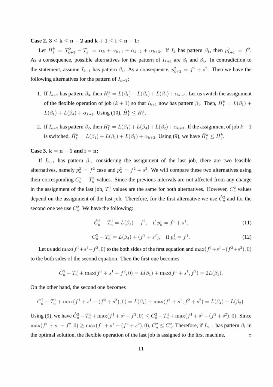
Case 3.k = n− 1 and i = n:

If In−1 has patternβ1, considering the assignment of the last job, there are two feasible

alternatives, namelyp2n = f 2 case andp2n = f 2 + s2. We will compare these two alternatives using

their correspondingC2n − T 1

n values. Since the previous intervals are not affected from any change

in the assignment of the last job,T 1n values are the same for both alternatives. However,C2

n values

depend on the assignment of the last job. Therefore, for the first alternative we useC2n and for the

second one we useC2n. We have the following:

C2n − T 1

n = L(β1) + f 2, if p1n = f 1 + s1, (11)

C2n − T 1

n = L(β4) + (f 2 + s2), if p1n = f 1. (12)

Let us addmax(f 1+s1−f 2, 0) to the both sides of the first equation andmax(f 1+s1−(f 2+s2), 0)

to the both sides of the second equation. Then the first one becomes

C2n − T 1

n +max(f 1 + s1 − f 2, 0) = L(β1) + max(f 1 + s1, f 2) = 2L(β1).

On the other hand, the second one becomes

C2n − T 1

n +max(f 1 + s1 − (f 2 + s2), 0) = L(β4) + max(f 1 + s1, f 2 + s2) = L(β4) + L(β2).

Using (9), we haveC2n−T 1

n +max(f 1+ s1− f 2, 0) ≤ C2n−T 1

n +max(f 1+ s1− (f 2+ s2), 0). Since

max(f 1 + s1 − f 2, 0) ≥ max(f 1 + s1 − (f 2 + s2), 0), C2n ≤ C2

n. Therefore, ifIn−1 has patternβ1 in

the optimal solution, the flexible operation of the last job is assigned to the first machine. 2

11

As a consequence of this lemma, if the flexible operations areassigned to the first machine for

two consecutive jobs (in such a case, there will be at least one interval with patternβ1), then in the

optimal schedule, the flexible operations must be assigned to the first machine for all jobs except the

first job. It is shown in Example 1 that in the optimal solutionthe first job need not have this property.

However, there are only two alternative assignments for this job which can be seen in Figure 1. Let

us define the following for notational simplicity:

σ1 = f 1 + f 2, σ2 = f 1 + s1 + f 2, σ3 = f 1 + f 2 + s2, σ4 = f 1 + s1 + f 2 + s2.

Then the corresponding makespan values for the two alternatives are as follows:

C1nb = σ2 + (n− 1)L(β1), if p11 = f 1 + s1, (13)

C2nb = σ1 + L(β2) + (n− 2)L(β1), if p11 = f 1. (14)

In these equations,Cknb is used to denote the makespan value for the no-buffer case for alternative

solutionk. The next lemma determines a special case where one of these two alternatives is optimal.

Lemma 3. If f 2 ≥ f 1 + s1, min{C1nb, C

2nb} is optimal.

Proof. Under the stated condition, even the flexible operation of a part is assigned to the first machine,

the processing time on the second machine is greater than total processing time on the first machine.

Therefore, interval lengths are determined byf 2. Using this, we can easily calculate a lower bound

for the optimal makespan. According to this, in order to minimize the lengths of the intervals, the

flexible operations must be assigned to the first machine for all jobs, except the first and the last ones.

Additionally, assigning the flexible operation of the last job to the second machine increases the length

of the last interval bys2 without changing any other. Therefore, the flexible operation of the last job

must also be assigned to the first machine. However, there is no such conclusion for the first job. As a

result, the lower bound of the optimal makespan ismin{f 1 + nf 2 + s1, f 1 + nf 2 + s2}. On the other

hand, we haveC1nb = f 1 + nf 2 + s1 andC2

nb = f 1 + nf 2 + s2. The minimum of these two values is

equal to the lower bound implying that one of these two alternatives is optimal. 2

The next lemma is a direct result of Lemma 2 and the reversibility property stated in Lemma 1

and thus the proof is omitted here.

Lemma 4. Given an optimal schedule, if there exists at least onek, 2 ≤ k ≤ (n − 1), such thatIk

has patternβ3, thenIi also has patternβ3 for all i = 2, 3, . . . , (n− 1).

12

Similar to the previous case, depending on the assignment ofthe flexible operation of the last job

we have two different alternatives with the following makespan values:

C3nb = σ3 + (n− 1)L(β3), if p1n = f 1, (15)

C4nb = σ1 + L(β2) + (n− 2)L(β3), if p1n = f 1 + s1. (16)

The following lemma determines a special condition similarto Lemma 3 where one of these two

alternatives is optimal.

Lemma 5. If f 1 ≥ f 2 + s2, min{C3nb, C

4nb} is optimal.

The proof is very similar to the proof of Lemma 3 and omitted here.

Lemma 6. Given an optimal schedule, if there exists at least onek, 3 ≤ k ≤ (n − 1), such thatIk

has either patternβ2 or β4, then the optimal solution is an alternating sequence ofβ2 andβ4 patterns

for intervals3, 4, . . . , (n− 1).

Proof. If Ik, k = 1, 2, . . . , (n − 1), has patternβ2, this means that the flexible operation is assigned

to the first machine for this job. Thus,p2k = f 2 which means thatI(k+1) cannot have patternβ2.

It can either beβ1 or β4. Lemmas 2 proves that if in an optimal scheduleIk has patternβ1 for

3 ≤ k ≤ (n− 1), then all intervals areβ1. Therefore, if there is an intervalIk, k = 1, 2, . . . , (n− 1)

with patternβ2 in an optimal schedule, then it must be followed byβ4. A similar reasoning proves

that aβ4 pattern must be followed by aβ2 pattern in an optimal schedule, which proves thatβ2 and

β4 patterns can only be sequenced alternatingly. 2

This lemma provides the optimal assignments for jobs3, 4, . . . , (n−1) if there exists at least oneβ2

or β4 pattern. For the remaining jobs (first, second and the last inthe sequence) depending on the two

possible assignments of the flexible operations there are a total of eight different solution alternatives.

Additionally, the makespan values of these alternatives depend also on whether the number of jobs

to be produced is even or odd. All possible solution alternatives and their corresponding makespan

values are summarized in Table 1. In this table the first threecolumns show the alternative assignments

of the flexible operations of jobs 1, 2, andn, respectively. An entry of “1” (“2”) in these columns

means the flexible operation is assigned to the first (second)machine for the corresponding job.

Let us consider two different solutions,A andB. B is said to dominateA, if makespan value

of A is greater than that ofB for all possible parameter values. A solution is called nondominated,

13

Assignment to M/c’s Cmax

Job1 1 Job2 2 Job n n = odd n = even

1 1 1 σ2 + 2L(β1) +(n−3)

2(L(β4) + L(β2)) σ2 + L(β1) +

(n−2)2

(L(β4) + L(β2))

1 1 2 σ4 + L(β1) +(n−1)

2L(β4) +

(n−3)2

L(β2) σ4 + L(β1) + L(β3) +(n−2)

2L(β4) +

(n−4)2

L(β2)

1 2 1 σ2 + (n−1)2

(L(β4) + L(β2)) σ2 + L(β1) +(n−2)

2(L(β4) + L(β2))

1 2 2 σ4 + L(β3) +(n−1)

2L(β4) +

(n−3)2

L(β2) σ4 + n

2L(β4) +

(n−2)2

L(β2)

2 1 1 σ1 + L(β1) +(n−3)

2L(β4) +

(n−1)2

L(β2) σ1 + (n−2)2

L(β4) +n

2L(β2)

2 1 2 σ3 +(n−1)

2(L(β4) + L(β2)) σ3 + L(β3) +

(n−2)2

(L(β4) + L(β2))

2 2 1 σ1 + L(β3) +(n−3)

2L(β4) +

(n−1)2

L(β2) σ1 + L(β1) + L(β3) +(n−4)

2L(β4) +

(n−2)2

L(β2)

2 2 2 σ3 + 2L(β3) +(n−3)

2(L(β4) + L(β2)) σ3 + L(β3) +

(n−2)2

(L(β4) + L(β2))

Table 1: Makespan values for the possible solution alternatives

if there exists no other solutions dominating this one. Onceit is proved that a solution is dominated

by another one, there is no need to consider this solution anymore. We compare the values given in

Table 1 with each other to determine the set of nondominated solution alternatives.

Let C ijk(l)nb denote the makespan value of the alternative in which the flexible operation of the

first job is assigned to machinei, the second to machinej, and thenth job to machinek, where

i, j, k ∈ {1, 2}. The superscriptl ∈ {e, o} denotes whether the total number of jobs to be processed,

n, is even or odd. As an example,C111(o)nb denotes the makespan value in which the flexible operations

are assigned to the first machine for jobs 1, 2, andn and there are an odd number of jobs to be

processed. Similarly,C212(e)nb denotes the makespan value in which the flexible operations are assigned

to the second machine for the first and the last jobs and to the first machine for the second job; there

are an even number of jobs to be processed.

In Table 1,C111(e)nb andC121(e)

nb have exactly the same makespan values. Similarly,C222(e)nb and

C212(e)nb have identical makespan values. Hence, without loss of generality, we will not considerC121(e)

nb

andC212(e)nb any more. In the following we will show thatC211(e)

nb is always smaller thanC112(e)nb ,

C122(e)nb , andC221(e)

nb . From Table 1 we have the following:

C211(e)nb

= σ1 +(n− 2)

2L(β4) +

n

2L(β2)

= f1 + f2 +(n− 2)

2max{f1, f2}+

n

2max{f1 + s1, f2 + s2}. (17)

14

C112(e)nb

: From Table 1 we have:

C112(e)nb

= σ4 + L(β1) + L(β3) +(n− 2)

2L(β4) +

(n− 4)

2L(β2)

= f1 + s1 + f2 + s2 +max{f1 + s1, f2}+max{f1, f2 + s2}

+(n− 2)

2max{f1, f2}+

(n− 4)

2max{f1 + s1, f2 + s2}.

Comparing this with (17):

C112(e)nb

− C211(e)nb

= s1 + s2 +max{f1 + s1, f2}+max{f1, f2 + s2} − 2max{f1 + s1, f2 + s2}

= max{f1 + s1 + s2, f2 + s2}+max{f1 + s1, f2 + s1 + s2} − 2max{f1 + s1, f2 + s2} ≥ 0.

C122(e)nb

: From Table 1 we have:

C122(e)nb

= f1 + s1 + f2 + s2 +n

2max{f1, f2}+

(n− 2)

2max{f1 + s1, f2 + s2}.

Comparing with (17) we have:

C122(e)nb

− C211(e)nb

= s1 + s2 +max{f1, f2} −max{f1 + s1, f2 + s2}

= max{f1 + s1 + s2, f2 + s1 + s2} −max{f1 + s1, f2 + s2} ≥ 0.

C221(e)nb

: From Table 1,C221(e)nb is equal to the following:

C221(e)nb

= f1 + f2 +max{f1 + s1, f2}+max{f1, f2 + s2}

+(n− 4)

2max{f1, f2}+

(n− 2)

2max{f1 + s1, f2 + s2}.

Then we have the following:

C221(e)nb

− C211(e)nb

= max{f1 + s1, f2}+max{f1, f2 + s2} −max{f1, f2} −max{f1 + s1, f2 + s2}

= max{2f1 + s1, f1 + s1 + f2 + s2, f1 + f2, 2f2 + s2} −max{2f1 + s1, f1 + f2 + s2, f1 + s1 + f2, 2f2 + s2}.

If we investigate the these two max statements term by term, we can conclude thatC221(e)nb ≥ C

211(e)nb .

For the remaining alternatives, whenn is even, there are no other dominance relations. This means

that, depending on the given parameter values, one of these nondominated alternatives can be optimal.

When there are an odd number of jobs to be produced, we will prove thatC211(o)nb is always smaller

thanC112(o)nb andC121(o)

nb , andC221(o)nb is always smaller thanC122(o)

nb andC212(o)nb . For this purpose, we

will use the following equations that we have in Table 1:

15

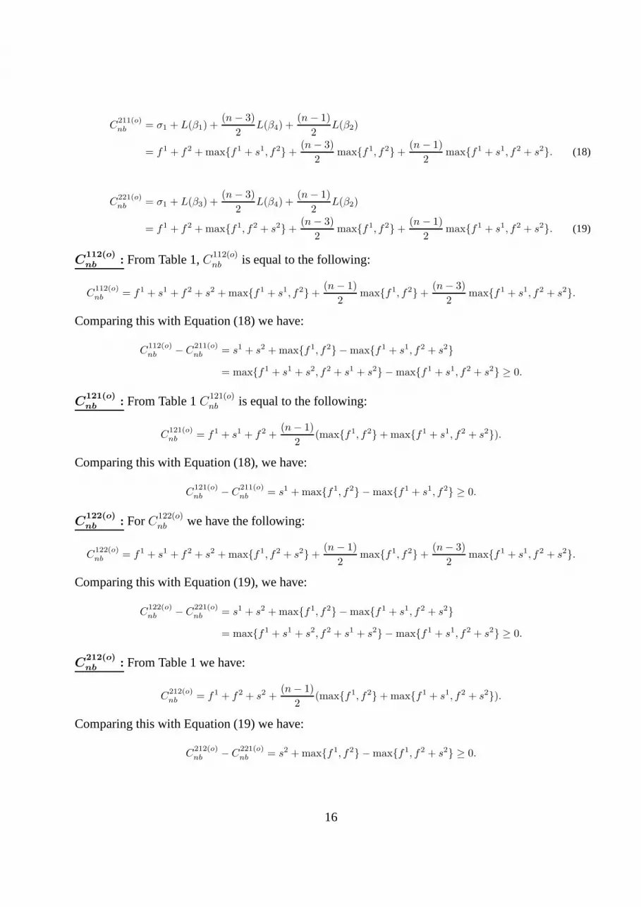
C211(o)nb

= σ1 + L(β1) +(n− 3)

2L(β4) +

(n− 1)

2L(β2)

= f1 + f2 +max{f1 + s1, f2}+(n− 3)

2max{f1, f2}+

(n− 1)

2max{f1 + s1, f2 + s2}. (18)

C221(o)nb

= σ1 + L(β3) +(n− 3)

2L(β4) +

(n− 1)

2L(β2)

= f1 + f2 +max{f1, f2 + s2}+(n− 3)

2max{f1, f2}+

(n− 1)

2max{f1 + s1, f2 + s2}. (19)

C112(o)nb

: From Table 1,C112(o)nb is equal to the following:

C112(o)nb

= f1 + s1 + f2 + s2 +max{f1 + s1, f2}+(n− 1)

2max{f1, f2}+

(n− 3)

2max{f1 + s1, f2 + s2}.

Comparing this with Equation (18) we have:

C112(o)nb

− C211(o)nb

= s1 + s2 +max{f1, f2} −max{f1 + s1, f2 + s2}

= max{f1 + s1 + s2, f2 + s1 + s2} −max{f1 + s1, f2 + s2} ≥ 0.

C121(o)nb

: From Table 1C121(o)nb is equal to the following:

C121(o)nb

= f1 + s1 + f2 +(n− 1)

2(max{f1, f2}+max{f1 + s1, f2 + s2}).

Comparing this with Equation (18), we have:

C121(o)nb

− C211(o)nb

= s1 +max{f1, f2} −max{f1 + s1, f2} ≥ 0.

C122(o)nb

: ForC122(o)nb we have the following:

C122(o)nb

= f1 + s1 + f2 + s2 +max{f1, f2 + s2}+(n− 1)

2max{f1, f2}+

(n− 3)

2max{f1 + s1, f2 + s2}.

Comparing this with Equation (19), we have:

C122(o)nb

− C221(o)nb

= s1 + s2 +max{f1, f2} −max{f1 + s1, f2 + s2}

= max{f1 + s1 + s2, f2 + s1 + s2} −max{f1 + s1, f2 + s2} ≥ 0.

C212(o)nb

: From Table 1 we have:

C212(o)nb

= f1 + f2 + s2 +(n− 1)

2(max{f1, f2}+max{f1 + s1, f2 + s2}).

Comparing this with Equation (19) we have:

C212(o)nb

− C221(o)nb

= s2 +max{f1, f2} −max{f1, f2 + s2} ≥ 0.

16

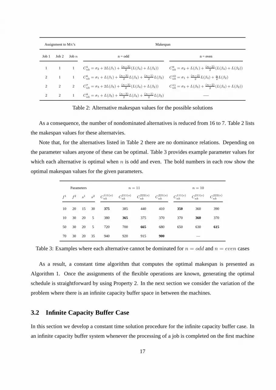
Assignment to M/c’s Makespan

Job 1 Job 2 Jobn n = odd n = even

1 1 1 C5nb

= σ2 + 2L(β1) +(n−3)

2(L(β4) + L(β2)) C9

nb= σ2 + L(β1) +

(n−2)2

(L(β4) + L(β2))

2 1 1 C6nb

= σ1 + L(β1) +(n−3)

2L(β4) +

(n−1)2

L(β2) C10nb

= σ1 +(n−2)

2L(β4) +

n

2L(β2)

2 2 2 C7nb

= σ3 + 2L(β3) +(n−3)

2(L(β4) + L(β2)) C11

nb= σ3 + L(β3) +

(n−2)2

(L(β4) + L(β2))

2 2 1 C8nb

= σ1 + L(β3) +(n−3)

2L(β4) +

(n−1)2

L(β2) —–

Table 2: Alternative makespan values for the possible solutions

As a consequence, the number of nondominated alternatives is reduced from 16 to 7. Table 2 lists

the makespan values for these alternatvies.

Note that, for the alternatives listed in Table 2 there are nodominance relations. Depending on

the parameter values anyone of these can be optimal. Table 3 provides example parameter values for

which each alternative is optimal whenn is odd and even. The bold numbers in each row show the

optimal makespan values for the given parameters.

Parameters n = 11 n = 10

f1 f2 s1 s2 C111(o)nb

C211(o)nb

C222(o)nb

C221(o)nb

C111(e)nb

C211(e)nb

C222(e)nb

10 20 15 30 375 385 440 410 350 360 390

10 30 20 5 380 365 375 370 370 360 370

50 30 20 5 720 700 665 680 650 630 615

70 30 20 35 940 920 915 900 —

Table 3: Examples where each alternative cannot be dominated for n = odd andn = even cases

As a result, a constant time algorithm that computes the optimal makespan is presented as

Algorithm 1. Once the assignments of the flexible operationsare known, generating the optimal

schedule is straightforward by using Property 2. In the nextsection we consider the variation of the

problem where there is an infinite capacity buffer space in between the machines.

3.2 Infinite Capacity Buffer Case

In this section we develop a constant time solution procedure for the infinite capacity buffer case. In

an infinite capacity buffer system whenever the processing of a job is completed on the first machine

17

Algorithm 1 Algorithm for the No-Buffer CaseInput: n, f 1, f 2, s1, ands2.

Output: C∗max.

1: if (f 2 ≥ f 1 + s1) then

2: C∗max = min{C1

nb, C2nb}.

3: else if(f 1 ≥ f 2 + s2) then

4: C∗max = min{C3

nb, C4nb}.

5: else if(n = odd)then

6: C∗max = min

i∈[1,8]{C i

nb}.

7: else

8: C∗max = min

i∈[1,4]∪[9,11]{C i

nb}.

9: end if

there is always an available space for this job in the buffer.Therefore, the first machine is never

blocked. If the optimal number of jobs for which the flexible operations are assigned to the first

machine is known, the optimal schedule can easily be generated using the SPT1-LPT2 algorithm

(Johnson’s algorithm [14]). According to this algorithm the jobs for which the processing times

on the first machine are less than that of the second machine are sequenced with respect to their

processing times on the first machine using the shortest processing time first method. The remaining

set of jobs are sequenced with respect to their processing times on the second machine using the

largest processing time first method. Afterwards, these twosequences are concatenated.

Our solution procedure relies on determining the number of jobs for which the flexible operations

are assigned to the first machine in the optimal schedule. Before going in to details of this procedure

let us first handle two special cases: Iff 1 ≥ f 2 + s2, then even if the flexible operations for all jobs

are assigned to the second machine, the processing times on the first machine are still greater than the

realized processing times on the second machine. Without considering the last job, this solution is the

best that can be achieved. The assignment for the last job need not be to the second machine resulting

from Example 1 and the reversibility property. There are twopossible assignment alternatives for this

job, which depend on the values ofs1 ands2. Let Ckinf denote the makespan value for alternativek

18

M1

M2

Time

p2

1

p1

n

p2

n

Cmax

T 1

2

T 2

1

C1

n

C2

n-1

C1

nT 1

2-

C2

n-1- T 2

1

……

Unavoidable idle

time

Unavoidable idle

time

p1

1

Figure 3: Minimizing makespan for infinite capacity buffer case

for the infinite buffer case. The corresponding makespan values for these alternatives are as follows:

C1inf = nf 1 + f 2 + s2, if p1n = f 1, (20)

C2inf = nf 1 + s1 + f 2, if p1n = f 1 + s1. (21)

When these two makespan values are compared with each other,if s1 > s2 (s1 < s2), then

assigning the flexible operation of the last job to the second(first) machine is optimal. If (s1 = s2)

both alternatives work equally well. Using the reversibility property, iff 2 ≥ f 1 + s1, then all flexible

operations are assigned to the first machine except the first job. Depending on the assignment of the

first job we have the following alternatives:

C3inf = f 1 + nf 2 + s2, if p11 = f 1, (22)

C4inf = f 1 + s1 + nf 2, if p11 = f 1 + s1. (23)

Let us now consider the case wheref 1 < f 2 + s2 andf 2 < f 1 + s1. Let r∗ denote the number

of jobs for which the flexible operations are assigned to the first machine. Since in this study, jobs

are identical, there are only two types of processing time values depending on the assignments:(f 1+

s1, f 2) and (f 1, f 2 + s2). Then, as a consequence of the Johnson’s algorithm ([14]),the flexible

operations are assigned to the second machine for the first (n − r∗) jobs and to the first machine for

the remainingr∗ jobs in the optimal schedule. We present this result as a property of the optimal

solutions for further reference in the text.

Property 3. In the optimal schedule, the flexible operations are assigned to the second machine for

the firstn− r∗ jobs and to the first machine for the lastr∗ jobs.

In the following, we develop a procedure to determine the value ofr∗. Observe that, the second

machine is idle during the first machine is processing the first job and similarly, the first machine is

19

idle during the second machine is processing the last job. These idle times are called unavoidable idle

times. Without considering these portions on both machines, as it is depicted in Figure 3, the rest of

the schedule is minimized when the total processing times onthe first and the second machines are as

close to each other as possible (the lower bound is attained when these two values are equal to each

other). That is, when|(C1n−T 1

2 )− (C2n−1−T 2

1 )| is minimized. The decision variables are the number

of flexible operations that must be assigned to the first and the second machines. Then, considering

all possible assignment alternatives for the first and the last jobs, which effect the unavoidable idle

times, the optimal makespan can be found. Hence, we need to evaluate the following alternatives:

1. If p11 = f 1 andp1n = f 1+ s1: Let r1 denote the number of jobs for which the flexible operations

are assigned to the first machine. Then, the total processingtimes on the two machines will be

equal if(n− 1)f 1 + r1s1 = (n− 1)f 2 + (n− r1)s

2. This yields the following:

r1 =(n− 1)(f 2 + s2 − f 1) + s2

s1 + s2.

By definition, r1 must be an integer. Then the optimal solution can be found by trying ⌊r1⌋

and⌈r1⌉ values and selecting the one with the smaller makespan value. ⌊a⌋ denotes the largest

integer value smaller thana and ⌈a⌉ denotes the smallest integer value larger thana. The,

corresponding makespan value is the following:

C5inf = min{nf 1 + ⌊r1⌋s

1 + f 2, f 1 + nf 2 + (n− ⌈r1⌉)s2}. (24)

2. If p11 = f 1 + s1 andp1n = f 1 + s1: Let r2 denote the number of jobs for which the flexible

operations are assigned to the first machine. Then, using similar arguments as above,(n −

1)f 1 + (r2 − 1)s1 = (n− 1)f 2 + (n− r2)s2. This yields the following:

r2 =(n− 1)(f 2 + s2 − f 1) + s1 + s2

s1 + s2.

The corresponding makespan value is the following:

C6inf = min{nf 1 + ⌊r2⌋s

1 + f 2, f 1 + s1 + nf 2 + (n− ⌈r2⌉)s2}. (25)

3. If p11 = f 1 andp1n = f 1: Denoting the number of jobs for which the flexible operations are

assigned to the first machine byr3, we must have(n−1)f 1+r3s1 = (n−1)f 2+(n−1−r3)s

2,

which gives the following:

r3 =(n− 1)(f 2 + s2 − f 1)

s1 + s2.

20

The corresponding makespan value is the following:

C7inf = min{nf 1 + ⌊r3⌋s

1 + f 2 + s2, f 1 + nf 2 + (n− ⌈r3⌉)s2}. (26)

4. If p11 = f 1+ s1 andp1n = f 1: Let r3 denote the number of jobs for which the flexible operations

are assigned to the first machine. Then, we must have(n− 1)f 1 + (r4 − 1)s1 = (n− 1)f 2 +

(n− 1− r4)s2. Therefore, we have the following:

r4 =(n− 1)(f 2 + s2 − f 1) + s1

s1 + s2.

The corresponding makespan value is the following:

C8inf = min{nf 1 + ⌊r4⌋s

1 + f 2 + s2, f 1 + s1 + nf 2 + (n− ⌈r4⌉)s2}. (27)

In Case 4 above, the unavoidable idle times on both machines are on their maximum values, which

increases the makespan value. The following lemma proves that this alternative cannot be optimal for

any parameter input.

Lemma 7. For any parameter inputmin{C5inf , C

6inf} ≤ C8

inf .

Proof. We will prove this lemma considering the following cases:

1. If s1 ≥ s2, thenr1 ≤ r4 ≤ r1 + 1. Let us compareC8inf with C5

inf given in Equation (24).

Comparing the first terms of the min functions of both equations, we havenf 1+ ⌊r4⌋s1+ f 2+

s2 ≥ nf 1+⌊r1⌋s1+f 2. When the second terms are compared with each other,f 1+s1+nf 2+

(n− ⌈r4⌉)s2 ≥ f 1 + s1 + nf 2 + (n− ⌈r1⌉ − 1)s2 ≥ f 1 + nf 2 + (n− ⌈r1⌉)s

2. Therefore, for

s1 ≥ s2, C8inf ≥ C5

inf .

2. If s1 < s2, thenr4 ≤ r2 ≤ r4 + 1. Let us compareC8inf with C6

inf given in Equation (25).

Comparing the first terms of the min functions of both equations, we havenf 1+ ⌊r2⌋s1+ f 2 ≤

nf 1+ (⌊r4⌋+1)s1+ f 2 < nf 1+ ⌊r4⌋s1 + f 2+ s2. When the second terms are compared with

each other,f 1 + s1 + nf 2 + (n − ⌈r4⌉)s2 ≥ f 1 + s1 + nf 2 + (n − ⌈r2⌉)s

2. Therefore, for

s1 < s2, C8inf ≥ C6

inf .

These two cases prove thatmin{C5inf , C

6inf} ≤ C8

inf . 2

21

In conclusion, the constant time algorithm for the infinite capacity buffer case is presented as

Algorithm 2. Note that, this algorithm outputs the minimum makespan values. In order to compute

these values, number of flexible operations that are assigned to the first and second machines are also

calculated. Using these together with Property 3 one can easily generate the optimal schedule (T ji

values fori = 1, 2, . . . , n andj = 1, 2).

Algorithm 2 Algorithm for the Infinite Capacity Buffer CaseInput: n, f 1, f 2, s1, ands2.

Output: C∗max.

1: if (f 1 ≥ f 2 + s2) then

2: C∗max = min{C1

inf , C2inf} given in Equations (20) and (21).

3: else if(f 2 ≥ f 1 + s1) then

4: C∗max = min{C3

inf , C4inf} given in Equations (22) and (23).

5: else

6: C∗max = min{C5

inf , C6inf , C

7inf} given in Equations (24), (25), and (26).

7: end if

After determining solution procedures for the no-buffer and infinite capacity buffer cases in this

section, the next section provides insights about the benefits of flexibility.

4 Managerial Insights

In the previous section we developed the algorithms that produce the optimal throughput rates for

given parameter values. This section analyzes benefits of flexibility and the conditions to attain

the maximum available benefit. We determine the cases (parameter values) under which a flexible

system is more beneficial than an inflexible one and the cases under which there are no benefits at

all. Furthermore, we seek answers to the following questions; where should we concentrate if we

want to increase the level of flexibility in the system? Is thefirst or the second machine the best

alternative in terms of throughput rate? What about the cost? How much flexibility do we really

need? Is it possible to quantify the value of additional flexibility? Answers to these questions are

especially important since without a clear understanding of the benefit associated with different levels

of flexibility, firms are reluctant to invest in flexibility ([19]).

22

For this analysis, we consider the option of increasing the level of flexibility in a classical inflexible

2-machine flowshop. If the workstations consist of CNC machines, the level of flexibility can be

increased by acquiring extra cutting tools and loading these on the tool magazines of both machines.

As a result, both machines are capable of processing the operations that require these tools. On the

other hand, if the workstations consist of manual operations, by cross-training the workers and placing

the necessary equipment to both of the workstations we transform the corresponding operations to

flexible. In conclusion, it is possible to increase the levelof flexibility in the system by some capital

investment plus annual costs such as the maintenance. Underthis setting, increasing the level of

flexibility means transforming some of the fixed operations to flexible ones. By this change, the fixed

operation time on the related machine reduces while the total processing time of the flexible operations

increases and the total processing times on the individual machines depend on the assignment of the

flexible operations.

The processing times of the operations are discrete values.When an operation is made flexible,

the corresponding processing time is transformed from fixedto flexible. For a given system there

is a finite number of alternatives for making the system flexible. This includes all combinations of

operations that a part requires. However, in order to deduceconclusions and make generalizations for

all problem types, we assume that the level of flexibility canbe increased to any value continuously,

not limited by discrete processing time values. The only constraint is, flexible processing time value

can not be greater than the original processing time of the machine in the fixed design.

For the classical system, the processing times of the machines are assumed to be fixed for all jobs

and denoted bypa for the first andpb for the second machine. The makespan value for this well

known classical manufacturing environment is denoted byCcmax. Let ǫi denote the processing time of

the flexible operations on machinei after the conversion is made. In order to have a meaningful

comparison, we assume that the total processing time that a part requires in the flexible system

is identical to that of an inflexible system, given that the flexible operations are assigned to the

machine they are converted from. Otherwise, technologicaldifference between the machines can

cause deviations. In order to satisfy this, if the second machine is used to increase the flexibility then

the processing times in the corresponding flexible system are f 1 = pa, f 2 = pb − ǫ2, s1 = ǫ1, and

s2 = ǫ2. If, on the other hand, the first machine is used for this purpose, the corresponding processing

times aref 1 = pa − ǫ1, f 2 = pb, s1 = ǫ1, ands2 = ǫ2.

Considering a flowshop system with partial resource flexibility where there aren jobs andm

23

machines Daniels et al. [9], concluded that a large portion of the available benefit associated with labor

flexibility can be realized with a relatively small investment in crosstraining. Similar conclusions are

also made by Jordan and Graves [15] and Nomden and van der Zee [17]. Our results in the current

study also support these conclusions, which are especiallyimportant when the cost associated with

increasing the level of flexibility is directly proportional with the level of flexibility itself. Under

such an assumption, since the marginal reduction in the makespan with respect to an increase in the

flexibility level is very small, but the increase in the corresponding cost is relatively high, a solution

with low flexibility level can be preferable to another solution with a high flexibility level. There are

some other cases where the cost is not directly proportionalto the level of flexibility. For example

a cutting tool associated with an operation with smaller processing time can be much more costly

than another one associated with a longer processing time. Hence, a higher flexibility level can be

preferable to lower levels in terms of both the makespan and the associated cost. In scheduling

literature, most of the studies address only a single criterion. However, most of the real-life problems

require multiple conflicting criteria and optimization of these simultaneously yields more realistic

schedules for the decision maker. We compare the original system with the flexible one in terms of

the makespan and determine the reduction in the makespan fordifferent parameter values. We will

comment on the associated cost of increasing the flexibilitylater on with the help of an example. We

denote the makespan of the flexible system byCfmax.

In this section, we consider the no-buffer and the infinite capacity buffer cases and analyze the

benefits of flexibility under different parameter values in each case. As mentioned before, the analysis

is made for the non-identical machines problem, which is more realistic than the identical machines

problem handled by Crama and Gultekin [6]. The identical machines problem is a special case of the

current one wheres1 = s2 = s. Therefore, the attained results throughout this section is valid for that

problem as well. Furthermore, by assuming the machines to benonidentical, we could see the effects

of technological differences between the machines to the benefits of flexibility.

Throughout the analysis, we assumed thatpa ≥ pb. The analysis and the results for the remaining

case is just the symmetric of this one as a consequence of the reversibility property.

The following lemma, which is valid for both the no-buffer and infinite capacity buffer cases,

proves that the benefits associated with flexibility is limited when the machine with smaller processing

time is used to increase the flexibility.

Lemma 8. If pa ≥ pb, then converting fixed operations to flexible ones from the second machine

24

reduces the makespan bymax{0, ǫ2 − ǫ1}.

Proof. For pa ≥ pb, independent of having a no-buffer or an infinite capacity buffer system, the

makespan of the inflexible system can easily be calculated tobe the following:

Ccmax = npa + pb. (28)

If fixed operations from the second machine with total processing time ofǫ2 are changed to be

flexible, thenf 1 = pa, f 2 = pb − ǫ2, s1 = ǫ1, ands2 = ǫ2. Sincepa ≥ pb, thenf 1 ≥ f 2 + s2. For

the no-buffer case, under the given condition, from Lemma 5,the minimum ofC3nb orC4

nb will be the

optimal solution. From Equation (15),C3nb = f 1 + f 2 + s2 + (n− 1)max{f 1, f 2 + s2} = npa + pb

and from Equation (16),C4nb = f 1 + f 2 + max{f 1 + s1, f 2 + s2} + (n − 2)max{f 1, f 2 + s2}} =

npa + pb + ǫ1 − ǫ2. Then, we have the following:

Ccmax −min{C3

nb, C4nb} = max{0, ǫ2 − ǫ1}.

For the infinite capacity buffer case, using Algorithm 2, theoptimal makespan is the minimum of

C1inf andC2

inf . From Equation (20),C1inf = nf 1 + f 2 + s2 = npa + pb and from Equation (21),

C2inf = nf 1 + s1 + f 2 = npa + ǫ1 + pb − ǫ2. Then, we have the following:

Ccmax −min{C1

inf , C2inf} = max{0, ǫ2 − ǫ1}. 2

As a consequence of this lemma, if the second machine is technologically new, (ǫ2 ≤ ǫ1), and the

processing time on this machine is smaller than the processing time on the first machine, then there

is no benefit of converting fixed operations from the second machine. On the other hand, if the first

machine has more advanced technology, then the reduction inthe makespan is equal to the difference

of the processing times of the flexible operations on both machines, (ǫ2 − ǫ1). Note that, this lemma

includespa = pb case, which can be rephrased as, if the processing times on both machines are equal

to each other, called perfect balance in the literature, then the benefit of increasing the flexibility using

the processing times of a single machine is limited.

As a consequence of Lemma 8, we only consider increasing the flexibility level using the

operations on the first machine. The processing times of the inflexible system arepa and pb and

the corresponding flexible ones aref 1 = pa− ǫ1, f 2 = pb, s1 = ǫ1, ands2 = ǫ2. We aim to determine

the gain in makespan quantified asCcmax − Cf

max for different parameter values. We analyze the

effects of the level of flexibility measured byǫ1, the imbalance between the machine processing times

25

0.5

0.75

1

2

Є1

s2/s1 Ratio

Cmax - Cmax

c f Cmax - Cmax

c f

1

1.2

1.5

3

pa/pb Ratio

Є1

a) Different s2/s1 ratios b) Different pa/pb ratios

Figure 4: Reduction in makespan with respect to the level of flexibility for no-buffer systems

measured bypa/pb, and the technological difference between the machines measured bys2/s1. For

pa ≥ pb, the makespan value of the classical system for both no-buffer and infinite capacity buffer

problems is equal toCcmax = npa+pb. For the no-buffer problem, the optimal solution for the flexible

system is found by using Algorithm 1 and for the infinite capacity buffer problem, it is found by using

Algorithm 2.

Figure 4a uses Algorithm 1 to depict the reduction in the makespan with respect to the flexibility

level. Different values are used for technological difference between the machines. In this graph

pa/pb ratio is fixed to 1.5. Since the graphs forn = odd andn = even cases are very similar to each

other, we only consider the former one here. According to this figure, the reduction in the makespan is

always greater when the second machine is technologically more advanced. In the figure, maximum

reduction is attained whens2/s1 = 0.5. Additionally, whatever the technological difference be,

Ccmax − Cf

max has a steep increase as the level of flexibility increases. After reaching a maximum

value for a relatively low level of flexibility, it starts decreasing. Therefore, it is not true that the gain

always increases as the level of flexibility increases. In the figure,s2/s1 = 1 case is identical to the

problem considered by Crama and Gultekin [6].

Similar conclusions can also be made for the infinite buffer case. Figure 5a depicts the same

graph for this system. This graph shows that most of the benefits associated with the flexibility can

be attained with a relatively small flexibility level. The greater the technological difference between

the machines, the greater the benefit of flexibility. Different than the no-buffer case,Ccmax − Cf

max

continues to increase slightly with respect toǫ1 with small fluctuations.

Figure 4b depicts the graph ofCcmax−Cf

max with respect toǫ1 for different values ofpa/pb. In this

26

Є1

0,5

0,75

1

2

s2/s1 Ratio

Cmax - Cmax

c f

1

1.2

1.5

3

pa/pb Ratio

Є1

Cmax - Cmax

c f

a) Different s2/s1 ratios b) Different pa/pb ratios

Figure 5: Reduction in makespan with respect to the level of flexibility for infinite buffer systems

graphs2/s1 is fixed to 0.75. We can see the effect of the imbalance betweenthe machine processing

times to the benefits of increasing flexibility. It can be concluded from this figure that the gain is

greater when the imbalance between the machine processing times are greater. Maximum reduction

is attained whenpa/pb = 3. Similar to the previous case, most of the gain in the makespan is attained

for low flexibility levels. When the processing times in the inflexible system are equal to each other,

pa/pb = 1, the benefit of flexibility is very limited as proven in Lemma 8.

Figure 5b depicts the same for the infinite capacity buffer case. Similar to the no-buffer case,

the benefits increase whenpa/pb increases. When the two processing times are equal to each other,

pa/pb = 1, the benefits are limited.

Figure 6 compares the no-buffer and infinite capacity buffersystems with each other with respect

to the flexibility level in the system. In this figurepa/pb = 1.5 ands2/s1 = 0.75. This figure shows

the effects of the additional buffer space to the system. Themaximum gain for the infinite capacity

buffer systems is greater than the maximum gain of the no-buffer systems. However, the gap between

the maximum gain of the infinite capacity and the maximum gainof the no-buffer systems is very

small. For low flexibility levels both systems perform equally well. Although in an infinite capacity

system, theoretically the buffer capacity must be at leastn− 1 parts, usually this maximum capacity

need not be used to get the optimal makespan value. Therefore, one can compare the cost of attaining

additional buffer space with the reduction in the makespan to design the production system.

The analysis in this section strengthen the conclusions of Daniels et al. [9] and Jordan and Graves

[15] who stated that a large portion of the available benefit associated with flexibility can be realized

with a relatively small flexibility level. However, the reduction in the makespan is not the only factor

27

Cmax

- Cmax

c f

No-

buffer

Infinite

buffer

Є1

Figure 6: Comparison of flexible no-buffer and infinite capacity buffer systems

for deciding the level of flexibility. The cost of increasingthe flexibility level is also important for

this decision. Considering the cost together with the makespan provides more insights to the decision

maker. In some production systems, the cost associated withincreasing the level of flexibility is

directly proportional with the level of flexibility itself.In such a production system, consider two

different flexibility levels,δ1 andδ2 such thatδ2 ≥ δ1. Solution corresponding toδ1 is better than

δ2, in terms of both makespan and cost, if the reduction in the makespan with respect toδ1 is not

less than the reduction inδ2. For such systems, the flexibility levels smaller than the points where

the reduction in makespan reaches its maximum value are the only alternative solutions. There is no

need to consider greater flexibility levels. However, the cost may not be directly proportional to the

flexibility level in some systems. The following is an example of such a situation.

Example 2. Let us consider the production of 20 identical jobs in a 2-machine no-buffer flowshop.

Each job requires 6 operations with corresponding processing times ofo1 = 3, o2 = 6, o3 = 8,

o4 = 13, o5 = 22, ando6 = 42 units. Assume that the second machine is capable of performing the

sixth operation and all remaining ones must be processed on the first machine. Therefore, we have

pa = 52 andpb = 42 units. Assume the second machine is more powerful and we haves2/s1 = 0.75.

Using (28), we haveCcmax = 1082. Assume that with some capital investment, the operations can be

made flexible. Let us suppose that the cost required to make each operation flexible is 2, 10, 7, 5, 12,

and 8, respectively. If the first operation is made flexible, sinceo1 = 3, the makespan of the flexible

system is given by Lemma 5 and Equation 15. The reduction in the makespan is equal to57.5 time

units and the corresponding cost is 2 in monetary units. Notethat, sincepa > pb ands2 ≤ s1, from

Lemma 8, converting the sixth operation into a flexible one does not reduce the makespan. Table 4

28

summarizes the costs and the makespan reductions for the alternatives. According to these, maximum

reduction in makespan is attained when the second operationis made flexible with a corresponding

cost of 10 units. If we compare the third and the fourth alternatives, the fourth alternative has a greater

reduction in makespan with a smaller cost, which means the fourth alternative dominates the third one.

The same alternative also dominates the fifth one. However, there are no dominance relations among

the boldly written remaining three alternatives. Each alternative is better than any other one either in

terms of the reduction in makespan or the associated cost.

Alternative Flexible Operation Reduction inCmax Cost

1 o1 57.5 2

2 o2 106 10

3 o3 80 7

4 o4 103 5

5 o5 47 12

Table 4: Reduction in the makespan and the associated costs for Example 2

For any given parameter values, such bi-criteria analysis considering the makespan and the cost

can easily be made by the methodology developed hereby. The increase in the throughput rate can be

compared with the capital investment and other relevant costs related with increasing the flexibility

level in the system through an engineering economic analysis.

5 Conclusion

In this study we considered machine flexibility as an option to increase the throughput rate in two

machine flowshops. As a consequence of this flexibility we assumed that each job has fixed and

flexible operations. We first considered the optimization problem where the machines are assumed

to be non-identical. For both the no buffer and infinite capacity buffer cases we developed constant

time solution procedures. In the second part, we demonstrated the benefits of machine flexibility.

We considered the reduction in the makespan corresponding to any flexibility level measured by the

processing time of the flexible operations. After this analysis we conclude that most of the benefits

in terms of the reduction in the makespan are attained with a relatively small level of flexibility. The

cost of increasing the flexibility level need not be directlyproportional with the flexibility level as

assumed in earlier studies. In such a situation, the optimalflexibility level can be determined through

a bicriteria analysis of the makespan and the cost as in Example 2.

29

This research can be extended by increasing the number of machines in the flowshop. In such

a case, different assumptions can be made regarding the flexible operations. For example, it can be

assumed that there is a flexible operation between any two adjacent machines. In another system,

the flexible operations can be assigned to any one of the machines in the system or to a subset of

machines, not necessarily consisting of adjacent machines. Determination of complexities of these

alternatives are open research questions. Furthermore, considering machine flexibility in different

production settings such as job shops or open shops and considering different objective functions

other than the makespan will also contribute to the literature.

Acknowledgments.The author thanks to anonymous referee whose constructive comments improved

the quality of the paper significantly. The author acknowledges the support of the Scientific and

Technical Research Council of Turkey under grant #110M489.

References

[1] R. Anuar and Y. Bukchin. Design and operation of dynamic assembly lines using worksharing.

International Journal of Production Research, 44:4043–4065, 2006.

[2] G.D. Batur, O.E. Karasan and M.S. Akturk. Multiple part-type scheduling in flexible robotic

cells. International Journal of Production Economics, 135:726–740, 2012.

[3] R. Beach, A.P. Muhlemann, D.H.R. Price, A. Paterson and J.A. Sharp. A review of

manufacturing flexibility.European Journal of Operational Research, 122(1):41–57, 2000.

[4] J. Browne, D. Dubois, K. Rathmill, S.P. Sethi and K.E. Stecke. Classification of flexible

manufacturing systems.The FMS Magazine, 2:114117, 1984.

[5] R.L. Burdett and E. Kozan. Sequencing and Scheduling in Flowshops with Task Redistribution.

The Journal of the Operational Research Society, 52(12):13791389, 2001.

[6] Y. Crama, H. Gultekin, Throughput Optimization in 2-Machine Flowshops with Flexible

Operations,Journal of Scheduling13(3): 227-243, 2010.

[7] Y. Crama, J. Van De Klundert and F.C.R. Spieksma, Production planning problems in printed

circuit board assembly,Discrete Applied Mathematics123:339–361, 2002.

30

[8] R.L. Daniels, J.B. Mazzola. Flow shop scheduling with resource flexibility. Operations

Research, 42:504–522, 1994.

[9] R.L. Daniels, J.B. Mazzola and D. Shi. Flow shop scheduling with partial resource flexibility.

Management Science, 50(5):658–669, 2004.

[10] A.E. Gray, A. Seidmann and K.E. Stecke. A Synthesis of Decision Models for Tool Management

in Automated Manufacturing.Management Science, 39(5):549–567, 1993.

[11] H. Gultekin, M.S. Akturk and O.E. Karasan. Cyclic scheduling of a robotic cell with tooling

constraints.European Journal of Operational Research, 174:777–796, 2006.

[12] H. Gultekin, M.S. Akturk and O.E. Karasan. Bi-criteriarobotic operation allocation in a flexible

manufacturing cell.Computers & Operations Research, 37:779-789, 2010.

[13] J.N.D. Gupta, C.P. Koulamas, G.J. Kyparisis, C.N. Potts and V.A. Strusevich. Scheduling

three-operation jobs in a two-machine flow shop to minimize makespan.Annals of Operations

Research, 129:171–185, 2004.

[14] S.M. Johnson. Optimal Two- and three-stage productionschedules with setup times included.

Naval Research Logistics Quarterly, 1:61-68, 1954.

[15] W.C. Jordan, S.C. Graves. Principles on the benefits of manufacturing process flexibility.

Management Science, 41(4):577–594, 1995.

[16] E. Muth. Reversibility property of production lines.Management Science, 25(2):152–158, 1979.

[17] G. Nomden, D.J. van der Zee. Virtual cellular manufacturing: Configuring routing flexibility.

International Journal of Production Economics, 112(1):439–451, 2008.

[18] M. Pinedo. Scheduling: Theory, Algorithms and Systems, 2nd edition. Prentice-Hall:

Englewood Cliffs, NJ, 2002.

[19] C. Tang, B. Tomlin. The power of flexibility for mitigating supply chain risks.International

Journal of Production Economics, 116(1):12–27, 2008.

[20] D. Upton. The management of manufacturing flexibility,California Management Review

Winter:72–89, 1994.

31