Scale-dependent correlations between soil heavy metals and As around four coal-fired power plants of...

ORIGINAL PAPER

Scale-dependent correlations between soil heavy metals and Asaround four coal-fired power plants of northern Greece

Nikos Nanos • Theodoros Grigoratos •

Jose Antonio Rodrıguez Martın • Constantini Samara

� Springer-Verlag Berlin Heidelberg 2014

Abstract We analyse the concentration of five trace

elements (As, Cu, Ni, Pb and Zn) in the topsoil of the

Kozani-Ptolemais basin where four coal-fired power plants

run to provide almost 47.8 % of electricity requirements in

Greece. We assume that if the power plants have altered

the spatial (co)variation of the analysed elements through

their toxic by-products, their effect would be observable

only on a small spatial scale, since deposition of airborne

pollutants is more evident if it is near the emission source.

We used Factorial Cokriging to estimate the small-scale

correlations among soil elements and to compare them to

large spatial-scale correlations. Soil samples were collected

from 92 sites. Given the low concentrations in soil heavy

metals and As, we observed no serious soil contamination

risk. We estimated correlations among the analysed ele-

ments on two spatial scales. On the larger scale, Ni and As

exhibited higher correlation and received higher weights

for the first regionalized factor, contrary to Cu, Pb and Zn

which weighted more for the second regionalized factor.

On the small spatial scale As associated with neither Ni nor

other heavy metals. We conclude that soil arsenic has been

altered by enrichment caused by some power plants

through fly ash deposition and/or disposal. However,

enrichment of soil elements was detectable only on the

smaller spatial scale because anthropogenic inputs in soil

through airborne emissions and subsequent deposition are

evident only in the vicinity of the emission source.

Keywords Factorial Cokriging � Fly ash � Geostatistics �Heavy metals � Multiscale variation � Soil pollution

1 Introduction

The natural concentration of metals and metalloids in soils,

known as heavy metals (HMs), depends primarily on

geological parent material composition (Alloway 1995;

Ramos-Miras et al. 2011; Roca-Perez et al. 2010; Wang

et al. 2011). However, in recent centuries, the concentra-

tion of HMs in soil has increased due to human inputs

stemming from several activities such as industry, power

generation or smelting (Colgan et al. 2003; Gao et al.

2013). More specifically, coal-fired power plants are

among the most relevant HMs sources in soil (Quick et al.

2003). The coal-fired power generating industry is likely to

emit not only fly ash, but also fugitive dust originating

from lignite transportation and ash disposal (Arditsoglou

et al. 2004; Samara 2005). As a result, several power plants

have enriched nearby soils with one or more heavy metals

or other potentially toxic elements; i.e., As, Cd, Pb and Ni

(Agrawal et al. 2010), Hg in China and Spain (Yang and

Wang 2008; Rodrıguez Martın et al. 2013) or As in Slo-

vakia (Keegan et al. 2006). Heavy metals emitted in a

gaseous form, or attached to fly ash, can travel thousands of

kilometres in the atmosphere before being deposited.

Electronic supplementary material The online version of thisarticle (doi:10.1007/s00477-014-0991-3) contains supplementarymaterial, which is available to authorized users.

N. Nanos (&)

Madrid Technical University, Ciudad Universitaria s/n,

28040 Madrid, Spain

e-mail: [email protected]

T. Grigoratos � C. Samara

Environmental Pollution Control Laboratory, Department

of Chemistry, Aristotle University of Thessaloniki,

54124 Thessaloniki, Greece

J. A. Rodrıguez Martın

Departamento de Medio Ambiente, Instituto Nacional de

Investigacion y Tecnologıa Agraria, 28040 Madrid, Spain

123

Stoch Environ Res Risk Assess

DOI 10.1007/s00477-014-0991-3

Author's personal copy

http://dx.doi.org/10.1007/s00477-014-0991-3

Nevertheless, the impact on soil is likely to be higher in the

vicinity of the emission source (Mandal and Sengupta

2006; Swaine 1994; Abbott et al. 2003; EHH Inc 2011).

The average deposition distance from the emission source

is linked to several parameters, including the pollutants

atmospheric residence time, the plant-specific characteris-

tics (i.e., height of stack), meteorological conditions and

topography (Agrawal et al. 2010; Godin Max et al. 1985).

Source identification of HMs in soil around power plants

is a challenge for environmental scientists since only the

sum of the two contributions (anthropogenic and natural) is

directly observable. However, the estimation of anthropo-

genic contribution is necessary prior to pollution preven-

tion and risk assessment (Christakos 1998). The statistical

methods that have been previously used to identify the

relevant sources of soil HMs include non-spatial techniques

such as multivariate analyses (Korre 1999), mixture mod-

elling (Portier 2001; Yu-Pin et al. 2010) or spatial methods

such as fractal analyses (Lima et al. 2003) and factorial

kriging, which employ the spatial distribution of the ana-

lysed HMs concentration to infer their sources in accor-

dance with the spatial scale (Goovaerts 1992; Holmes et al.

2005; Nanos and Rodrıguez Martın 2012; Rodrıguez et al.

2008; Rodrıguez Martin et al. 2014; Lv et al. 2013).

In the Kozani-Ptolemais basin (northern Greece), four

coal-fired power plants (4,000 MW) have been installed

since 1950 which cover almost 47.8 % of electricity

demands in Greece. In addition, three coal-mine complexes,

with total reserves of 2.3 billion t, provide the necessary fuel

to the four power stations. In the past, the area has suffered

from high levels of airborne particles and heavy metals

(Stalikas et al. 1997). In recent years, all the power plants

are equipped with electrostatic precipitators with high

retention efficiency ([99.9 %). However, considerable

amounts of fine fly ash particles may be emitted to the

atmosphere because of the high rate of coal consumption. In

addition to stack emissions, another significant particle

source is fugitive dust originating from the mining process,

including emissions from mining equipment, translocation

of soil or coal, vehicle traffic on unpaved roads, transpor-

tation and deposition of lignite and lignite ash. Fugitive dust

generated from the above operations, affects primarily the

areas close to the mines and the power stations (Petaloti

et al. 2003; Triantafyllou 2003). Since this is one of the most

prone areas to pollutants emission, several results for both

soil and air pollution assessments have been published

(Georgakopoulos et al. 2002a, b; Samara 2005; Triantafyllou

2003). In the first study on soil heavy metals distribution,

Stalikas et al. (1997) reported relative Ni and Cr enrichment,

but no enrichment for Pb, Zn and Cu. Fifteen years later,

Petrotou et al. (2012) reported that four heavy metals (Cu,

Cd, Pb and Zn) had been enriched in soil due to either

agrochemical inputs or fly ash deposition in the vicinity of

some power plants (unlike Ni and Cr, which were deemed of

natural origin). Georgakopoulos et al. 2002a stated that a

mixed lithogenic and anthropogenic origin for some metals

(Ni, Zn, Cr) and a purely anthropogenic origin for Se. In

recent study Rodrıguez Martin et al. (2014) report low

concentrations of soil Hg around the four coal-fired power

plants.

In the present study, we analysed the spatial (co)varia-

tion of four heavy metals (Cu, Ni, Pb and Zn) and As in 92

samples collected from the vicinity of these power plants.

We assumed that if the power plants have altered the

spatial (co)variation of the analysed elements, their effect

would be observable only on a small spatial scale. We used

factorial kriging analysis to estimate the small-scale cor-

relations among soil elements and to compare them to

large-scale correlations where the influence of the power

plants is typically diminished.

2 Materials and methods

2.1 Study area and sampling

The soils of the Kozani-Ptolemais basin have developed as

alluvial fans. Their texture is variable (characterized fre-

quently as sandy or clayley-silty) and according to the

USDA soil taxonomy they belong to Alfisol (D.E.H. 2010).

The soil pH presents a significant variation (range 4–9)

being more acidic in the north-western part of the basin. In

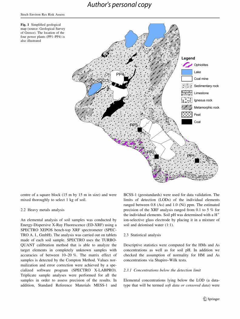
the northern part of the study area (Fig. 1), metamorphic

geological features predominate: schist and flysch in the

northwest and marbles in the northeast. To the south, there

is a gradual tendency for calcareous limestone to dominate

in conjunction with ophiolitic rocks. However, the vast

majority of the study area consists of sedimentary rocks of

mixed (or unknown) geological origin. Traditionally, the

soils in this area have been used for crop production

(predominantly wheat and corn but also fruit trees and

potatoes) and for sheep husbandry. The climate is conti-

nental Mediterranean and is characterized by low winter

temperatures (-1.3–6.3 �C) and high summer temperatures

(20.1–28.5 �C). Prevailing winds are weak to moderate and

blow mostly along the NW/SE axis of the basin as a result

of the channelled synoptic wind (Triantafyllou 2003).

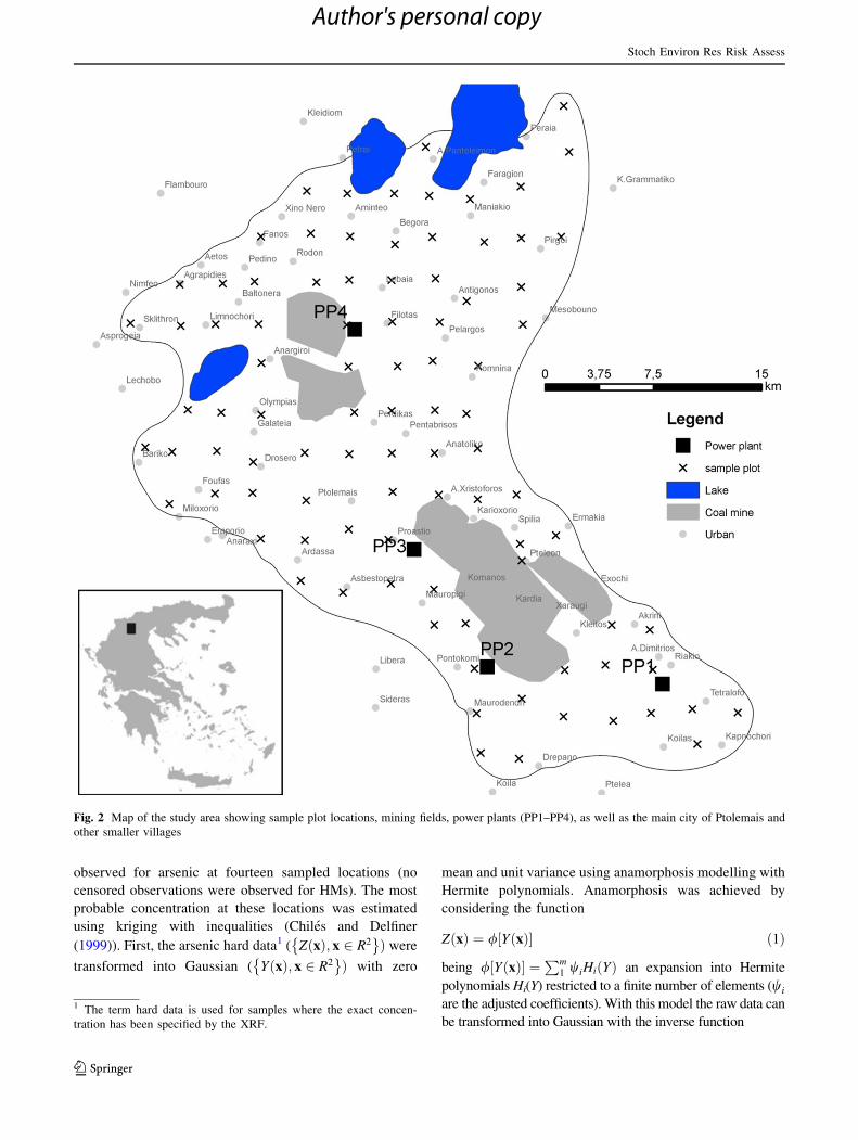
Soil samples were collected in January 2011 from 92

locations (Fig. 2). A systematic grid (3 km by 3 km in

size) was first overlaid over the basin surface and a sam-

pling plot was established at the grid nodes when at least

one wheat field was visible (in the ortho-photograph)

within a 600-m distance from the grid node. Samples were

collected from the closest wheat field to the grid node from

the 20 cm topmost soil layer. At each sampling site, five

subsamples were taken from the four vertexes and the


123


centre of a square block (15 m by 15 m in size) and were

mixed thoroughly to select 1 kg of soil.

2.2 Heavy metals analysis

An elemental analysis of soil samples was conducted by

Energy-Dispersive X-Ray Fluorescence (ED-XRF) using a

SPECTRO XEPOS bench-top XRF spectrometer (SPEC-

TRO A. I., GmbH). The analysis was carried out on tablets

made of each soil sample. SPECTRO uses the TURBO-

QUANT calibration method that is able to analyze the

target elements in completely unknown samples with

accuracies of between 10–20 %. The matrix effect of

samples is detected by the Compton Method. Values nor-

malization and error correction were achieved by a spe-

cialized software program (SPECTRO X-LABPRO).

Triplicate sample analyses were performed for all the

samples in order to assess precision of the results. In

addition, Standard Reference Materials MESS-1 and

BCSS-1 (geostandards) were used for data validation. The

limits of detection (LODs) of the individual elements

ranged between 0.8 (As) and 1.0 (Ni) ppm. The estimated

precision of the XRF analysis ranged from 0.1 to 5 % for

the individual elements. Soil pH was determined with a H?

ion-selective glass electrode by placing it in a mixture of

soil and deionised water (1:1).

2.3 Statistical analysis

Descriptive statistics were computed for the HMs and As

concentrations as well as for soil pH. In addition we

checked the assumption of normality for HM and As

concentrations via Shapiro–Wilk tests.

2.3.1 Concentrations below the detection limit

Elemental concentrations lying below the LOD (a data-

type that will be termed soft data or censored data) were

Fig. 1 Simplified geological

map (source: Geological Survey

of Greece). The location of the

four power plants (PP1–PP4) is

also illustrated


123


observed for arsenic at fourteen sampled locations (no

censored observations were observed for HMs). The most

probable concentration at these locations was estimated

using kriging with inequalities (Chiles and Delfiner

(1999)). First, the arsenic hard data1 ( Z xð Þ; x 2 R2� �

Þ were

transformed into Gaussian ( Y xð Þ; x 2 R2� �

Þ with zero

mean and unit variance using anamorphosis modelling with

Hermite polynomials. Anamorphosis was achieved by

considering the function

Z xð Þ ¼ / Y xð Þ½ � ð1Þ

being / Y xð Þ½ � ¼Pm

1 wiHi Yð Þ an expansion into Hermite

polynomials Hi(Y) restricted to a finite number of elements (wi

are the adjusted coefficients). With this model the raw data can

be transformed into Gaussian with the inverse function

Fig. 2 Map of the study area showing sample plot locations, mining fields, power plants (PP1–PP4), as well as the main city of Ptolemais and

other smaller villages

1 The term hard data is used for samples where the exact concen-

tration has been specified by the XRF.


123


Y xð Þ ¼ /�1 Z xð Þ½ � ð2Þ

Subsequently, the experimental variogram for the

Gaussian-transformed hard-data was computed (78 samples

were available for variogram computation) and a model was

adjusted to the experimental variogram. In addition, we

transformed the LOD at the censored data locations using the

anamorphosis model build previously (in order to constrain

the simulated data interval at the maximum permissible

value defined by the XRFs detection limit).

Finally, soft arsenic data were replaced with a simulated

dataset by computing the conditional expectation of the

target variable at each censored-data location. Simulations

were in accordance with the variogram model and were

also conditioned by the censoring interval (i.e. the Gauss-

ian-transformed LOD) and the surrounding hard data. To

calculate the conditional expectation, we ran 1000 real-

izations of the target (Gaussian) variable using a Gibbs

sampler implemented in Isatis (2008). The expected As

values at soft data locations were finally backtransformed

to the initial scale using Eq. 1.

2.3.2 Principal components analysis

Principal components analysis (PCA) was used to display

the most relevant multivariate correlations among soil

heavy metals and As. Prior to PCA, we centred and stan-

dardized (to unit variance) the HMs and As concentrations

(for As we used 78 hard data and 14 back-transformed soft

data). Subsequently, Pearson-correlation coefficients were

computed between soil heavy metals and arsenic concen-

trations and were arranged in matrix form to run the PCA.

A correlation circle was computed by estimating the cor-

relation between the first two principal components and the

original variables.

2.3.3 Factorial Cokriging

The HMs and As concentrations were further analyzed to

compute multiscale correlations via Factorial Cokriging

(Chiles and Delfiner 1999). The statistical details of this

method have been described elsewhere (Goovaerts 1992).

Here we present only the main steps:

Step 1. Raw data for HMs and for As were transformed

to Gaussian using the anamorphosis modelling with

Hermite polynomials procedure (see Sect. 2.3.1). The As

data set included not only the concentrations at hard-data

locations but also the estimated As concentrations at

soft-data locations (bellow the LOD).

Step 2. Computations in this step included not only the

experimental variogram calculation for each element

separately, but also the computation of the cross

variograms for each element combination (see also Olea

(2006) for a comprehensive presentation on variogram

analysis).

Step 3. The fifteen experimental variograms were mod-

elled using a Linear Model of Coregionalisation (LMC)

with three variogram structures (the specific LMC char-

acteristics are presented in the Results section). The LMC

parameters were adjusted to the experimental variograms

by an iterative algorithm implemented in Isatis (Lajaunie

and Behaxeteguy 1989; Isatis 2008).

Step 4. Before using the LMC for further calculations,

the goodness of prediction was evaluated via cross-

validation.

Step 5. Subsequently, we arranged the LMC partial sill

parameters in matrix form and we constructed the

coregionalisation matrix for each structure. A coregio-

nalisation matrix for structure k is a symmetric matrix

(analogous to the variance–covariance matrix) with

diagonal and off-diagonal elements the partial sill of

the auto- and cross-variogram models, respectively

(estimated through the LMC).

Finally we run a PCA for each coregionalisation matrix

separately and we obtained the scale-dependent Re-

gionalised Factors (RF). An RF is a model-derived

unobserved spatial variable that is specific to the kth

spatial scale, which results from decomposing the

original variables into a basis of random variables for

each spatial scale of variation, which are stationary and

uncorrelated. The pair of correlation coefficients

between the first two RFs and the original variables

was plotted on a circle of correlation (exactly as in the

PCA but specifically for each spatial scale).

Step 6. RF scores were estimated on both the sampled

locations and a regular grid over the study area using a

modified cokriging system of equations. This technique

differs from classical cokriging in two aspects (Wack-

ernagel 2003): First, in the right hand side of the

cokriging system of equations the transformation coef-

ficients of the factor of interest are multiplied by the

values of the spatial correlation function (which

describes the correlation at the scale of interest). In

addition, cokriging weights (assigned to data locations)

sum up to 0.

Step 7. In the last step we estimated HMs and As

concentrations on a regular grid over the study area. We

used the previously adjusted LMC (see steps 2 and 3)

and ordinary cokriging to produce the Gaussian esti-

mates of the variables. Finally, we back-transformed—

from the Gaussian to the raw scale—the resulting

estimates using Eq. 1. During back-transformation we

set the authorized interval on the raw data to the

minimum and maximum concentrations for each ele-

ment separately (see Table 1).


123


3 Results

3.1 Soil HMs contents

A statistical summary for pH and the analysed elements is

presented in Table 1. The null hypothesis of normality was

rejected for nickel, arsenic and copper but zinc and lead may be

considered normally distributed (Table 1). Content decreases

in the following order: Ni � Zn[Cu[Pb � As. Nickel

content was very high in several locations and exceeded the

corresponding threshold value for European soils in 68 samples

(Gawlik and Bidoglio 2006). Arsenic was detectable in 78

samples but concentrations lying bellow the LOD were

recovered using kriging with inequalities (see Online Resource

1). In 74 samples, As concentration was lower than

9.4 mg kg-1 and exceeded 15 mg kg-1 in only 4 samples

(mostly located around P1, see Online resource 1). The average

As concentration (4.4 mg kg-1) fell within the worldwide

acceptable limits (between 0.2 and 40 mg kg-1 according to

Moreno-Jimenez et al. 2012). The average concentrations of

Cu, Pb and Zn (29.1, 17.6 and 57.3 mg kg-1 respectively) were

not very high and did not exceed the threshold values reported

for European soils (Gawlik and Bidoglio 2006).

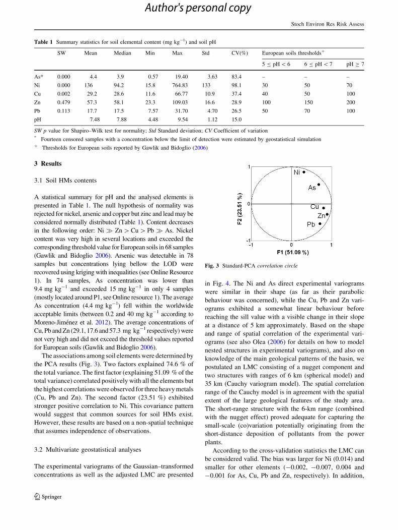
The associations among soil elements were determined by

the PCA results (Fig. 3). Two factors explained 74.6 % of

the total variance. The first factor (explaining 51.09 % of the

total variance) correlated positively with all the elements but

the highest correlations were observed for three heavy metals

(Cu, Pb and Zn). The second factor (23.51 %) exhibited

stronger positive correlation to Ni. This covariance pattern

would suggest that common sources for soil HMs exist.

However, these results are based on a non-spatial technique

that assumes independence of observations.

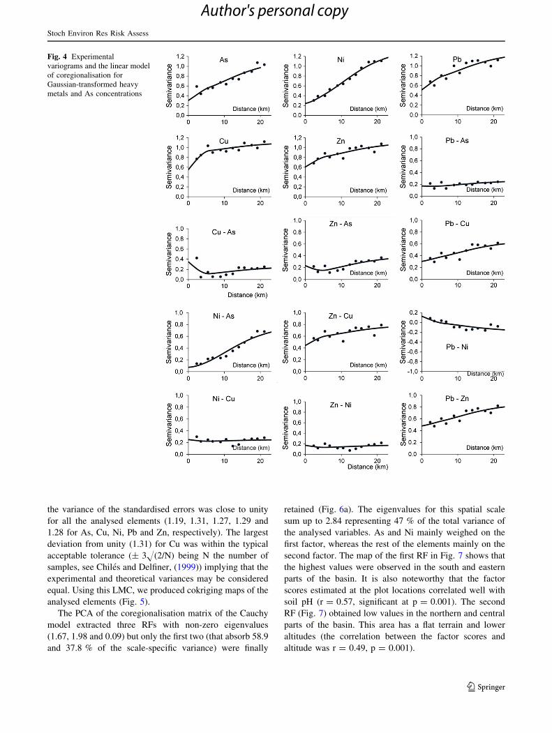
3.2 Multivariate geostatistical analyses

The experimental variograms of the Gaussian–transformed

concentrations as well as the adjusted LMC are presented

in Fig. 4. The Ni and As direct experimental variograms

were similar in their shape (as far as their parabolic

behaviour was concerned), while the Cu, Pb and Zn vari-

ograms exhibited a somewhat linear behaviour before

reaching the sill value with a visible change in their slope

at a distance of 5 km approximately. Based on the shape

and range of spatial correlation of the experimental vari-

ograms (see also Olea (2006) for details on how to model

nested structures in experimental variograms), and also on

knowledge of the main geological patterns of the basin, we

postulated an LMC consisting of a nugget component and

two structures with ranges of 6 km (spherical model) and

35 km (Cauchy variogram model). The spatial correlation

range of the Cauchy model is in agreement with the spatial

extent of the large geological features of the study area.

The short-range structure with the 6-km range (combined

with the nugget effect) proved adequate for capturing the

small-scale (co)variation potentially originating from the

short-distance deposition of pollutants from the power

plants.

According to the cross-validation statistics the LMC can

be considered valid. The bias was larger for Ni (0.014) and

smaller for other elements (-0.002, -0.007, 0.004 and

-0.001 for As, Cu, Pb and Zn, respectively). In addition,

Table 1 Summary statistics for soil elemental content (mg kg-1) and soil pH

SW Mean Median Min Max Std CV(%) European soils thresholds?

5 B pH \ 6 6 B pH \ 7 pH C 7

As* 0.000 4.4 3.9 0.57 19.40 3.63 83.4 – – –

Ni 0.000 136 94.2 15.8 764.83 133 98.1 30 50 70

Cu 0.002 29.2 28.6 11.6 66.77 10.9 37.4 40 50 100

Zn 0.479 57.3 58.1 23.3 109.03 16.6 28.9 100 150 200

Pb 0.113 17.7 17.5 7.57 31.70 4.70 26.5 50 70 100

pH 7.48 7.88 4.48 9.54 1.12 15.0

SW p value for Shapiro–Wilk test for normality; Std Standard deviation; CV Coefficient of variation* Fourteen censored samples with a concentration below the limit of detection were estimated by geostatistical simulation? Thresholds for European soils reported by Gawlik and Bidoglio (2006)

Fig. 3 Standard-PCA correlation circle


123


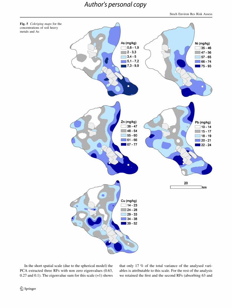
the variance of the standardised errors was close to unity

for all the analysed elements (1.19, 1.31, 1.27, 1.29 and

1.28 for As, Cu, Ni, Pb and Zn, respectively). The largest

deviation from unity (1.31) for Cu was within the typical

acceptable tolerance (± 3H(2/N) being N the number of

samples, see Chiles and Delfiner, (1999)) implying that the

experimental and theoretical variances may be considered

equal. Using this LMC, we produced cokriging maps of the

analysed elements (Fig. 5).

The PCA of the coregionalisation matrix of the Cauchy

model extracted three RFs with non-zero eigenvalues

(1.67, 1.98 and 0.09) but only the first two (that absorb 58.9

and 37.8 % of the scale-specific variance) were finally

retained (Fig. 6a). The eigenvalues for this spatial scale

sum up to 2.84 representing 47 % of the total variance of

the analysed variables. As and Ni mainly weighed on the

first factor, whereas the rest of the elements mainly on the

second factor. The map of the first RF in Fig. 7 shows that

the highest values were observed in the south and eastern

parts of the basin. It is also noteworthy that the factor

scores estimated at the plot locations correlated well with

soil pH (r = 0.57, significant at p = 0.001). The second

RF (Fig. 7) obtained low values in the northern and central

parts of the basin. This area has a flat terrain and lower

altitudes (the correlation between the factor scores and

altitude was r = 0.49, p = 0.001).

Fig. 4 Experimental

variograms and the linear model

of coregionalisation for

Gaussian-transformed heavy

metals and As concentrations


123


In the short spatial scale (due to the spherical model) the

PCA extracted three RFs with non zero eigenvalues (0.63,

0.27 and 0.1). The eigenvalue sum for this scale (=1) shows

that only 17 % of the total variance of the analysed vari-

ables is attributable to this scale. For the rest of the analysis

we retained the first and the second RFs (absorbing 63 and

Fig. 5 Cokriging maps for the

concentrations of soil heavy

metals and As


123


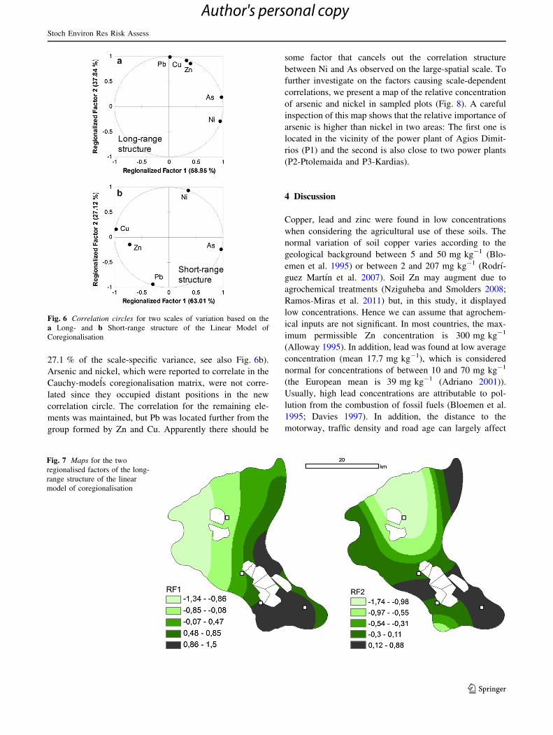
27.1 % of the scale-specific variance, see also Fig. 6b).

Arsenic and nickel, which were reported to correlate in the

Cauchy-models coregionalisation matrix, were not corre-

lated since they occupied distant positions in the new

correlation circle. The correlation for the remaining ele-

ments was maintained, but Pb was located further from the

group formed by Zn and Cu. Apparently there should be

some factor that cancels out the correlation structure

between Ni and As observed on the large-spatial scale. To

further investigate on the factors causing scale-dependent

correlations, we present a map of the relative concentration

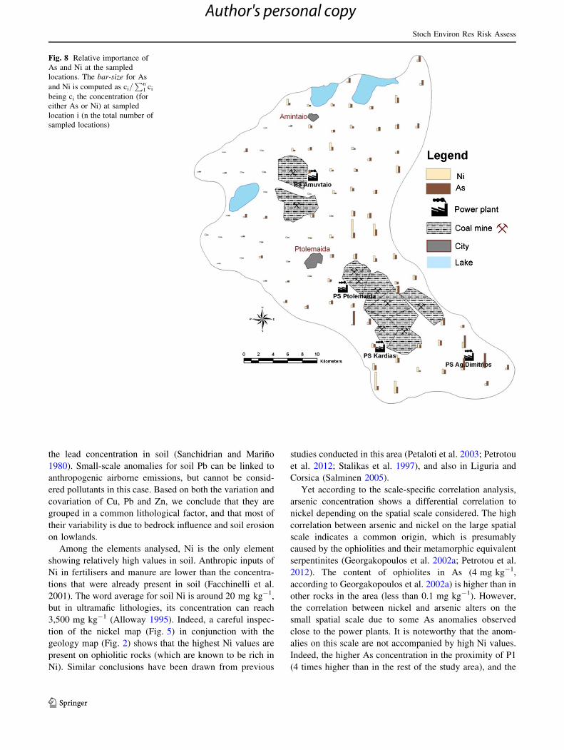
of arsenic and nickel in sampled plots (Fig. 8). A careful

inspection of this map shows that the relative importance of

arsenic is higher than nickel in two areas: The first one is

located in the vicinity of the power plant of Agios Dimit-

rios (P1) and the second is also close to two power plants

(P2-Ptolemaida and P3-Kardias).

4 Discussion

Copper, lead and zinc were found in low concentrations

when considering the agricultural use of these soils. The

normal variation of soil copper varies according to the

geological background between 5 and 50 mg kg-1 (Blo-

emen et al. 1995) or between 2 and 207 mg kg-1 (Rodrı-

guez Martın et al. 2007). Soil Zn may augment due to

agrochemical treatments (Nziguheba and Smolders 2008;

Ramos-Miras et al. 2011) but, in this study, it displayed

low concentrations. Hence we can assume that agrochem-

ical inputs are not significant. In most countries, the max-

imum permissible Zn concentration is 300 mg kg-1

(Alloway 1995). In addition, lead was found at low average

concentration (mean 17.7 mg kg-1), which is considered

normal for concentrations of between 10 and 70 mg kg-1

(the European mean is 39 mg kg-1 (Adriano 2001)).

Usually, high lead concentrations are attributable to pol-

lution from the combustion of fossil fuels (Bloemen et al.

1995; Davies 1997). In addition, the distance to the

motorway, traffic density and road age can largely affect

Fig. 6 Correlation circles for two scales of variation based on the

a Long- and b Short-range structure of the Linear Model of

Coregionalisation

Fig. 7 Maps for the two

regionalised factors of the long-

range structure of the linear

model of coregionalisation


123


the lead concentration in soil (Sanchidrian and Marino

1980). Small-scale anomalies for soil Pb can be linked to

anthropogenic airborne emissions, but cannot be consid-

ered pollutants in this case. Based on both the variation and

covariation of Cu, Pb and Zn, we conclude that they are

grouped in a common lithological factor, and that most of

their variability is due to bedrock influence and soil erosion

on lowlands.

Among the elements analysed, Ni is the only element

showing relatively high values in soil. Anthropic inputs of

Ni in fertilisers and manure are lower than the concentra-

tions that were already present in soil (Facchinelli et al.

2001). The word average for soil Ni is around 20 mg kg-1,

but in ultramafic lithologies, its concentration can reach

3,500 mg kg-1 (Alloway 1995). Indeed, a careful inspec-

tion of the nickel map (Fig. 5) in conjunction with the

geology map (Fig. 2) shows that the highest Ni values are

present on ophiolitic rocks (which are known to be rich in

Ni). Similar conclusions have been drawn from previous

studies conducted in this area (Petaloti et al. 2003; Petrotou

et al. 2012; Stalikas et al. 1997), and also in Liguria and

Corsica (Salminen 2005).

Yet according to the scale-specific correlation analysis,

arsenic concentration shows a differential correlation to

nickel depending on the spatial scale considered. The high

correlation between arsenic and nickel on the large spatial

scale indicates a common origin, which is presumably

caused by the ophiolities and their metamorphic equivalent

serpentinites (Georgakopoulos et al. 2002a; Petrotou et al.

2012). The content of ophiolites in As (4 mg kg-1,

according to Georgakopoulos et al. 2002a) is higher than in

other rocks in the area (less than 0.1 mg kg-1). However,

the correlation between nickel and arsenic alters on the

small spatial scale due to some As anomalies observed

close to the power plants. It is noteworthy that the anom-

alies on this scale are not accompanied by high Ni values.

Indeed, the higher As concentration in the proximity of P1

(4 times higher than in the rest of the study area), and the

Fig. 8 Relative importance of

As and Ni at the sampled

locations. The bar-size for As

and Ni is computed as ci=Pn

1 ci

being ci the concentration (for

either As or Ni) at sampled

location i (n the total number of

sampled locations)


123


fact that it is also close to P2 and P3, suggest local

enrichment due to power plant emissions. Modis and Va-

talis (2013) report similar As-enrichment in the soil of the

basin of Kozani-Ptolemais caused by the power plants (but

see also Gamaletsos et al. 2013). Similar effects were

observed at the Slovakian Electrarne Novaky, which has

been found to be responsible for soil As enrichment at up to

5 km from the source (Keegan et al. 2006). Elsewhere,

coal-fired power plants have been found to be responsible

for soil enrichment with several heavy metals, including As

(Agrawal et al. 2010; Gao et al. 2013, Mandal and Seng-

upta 2006). Arsenic and other elements volatilised during

coal combustion (i.e., Se and Br) come into contact with fly

ash that due to its large specific area, it is finally enriched

before escaping the stack. Given its high volatility, As is

emitted to the atmosphere from power plants to a large

extent (Reddy et al. 2005). In fact, coal combustion is the

second most important anthropogenic source of As in the

atmosphere (Alloway 1995).

Several studies done in the same area have shown that

the fly ash from power plants is rich in As. Depending on

the power plant the fly ash content can be between 5 and 10

times richer in As than average soil content. Georgako-

poulos et al. (2002b) reported that the fly ash from P1

was twice as rich in arsenic as compared to the rest of the

power plants (38.8 mg kg-1 in P1 versus 27.2, 20.8 and

20.5 mg kg-1 in P2, P3 and P4, respectively). Samara

(2005) found a similar As content in the fly ashes from P1

and P2 (46.9 mg kg-1), which was higher than those of the

fly ashes from P3 and P4 (40 and 27 mg kg-1, respec-

tively). In addition, the feedstock lignite of P1 has a higher

As content (11.1 mg kg-1) if compared to the other plants

(8.9, 7.3 and 5.7 mg kg-1 in P2, P3 and P4, respectively

(Samara 2005)). Finally, the local circulation systems

induced by topographic complexity, the marked roughness

of the terrain, and the channelled synoptic wind along its

NW/SE axis (Triantafyllou 2003) certainly affect the dis-

persion of air pollutants by possibly favouring greater

deposition close to P1. Unlike P1, the As concentration

around P4 (located in the northern part of the study area,

Fig. 5) was particularly low (not higher than 3.4 mg kg-1).

Apparently, this is the result of the local meteorological

conditions and the lower annual emission of fly ash at the

P4 power plant (Samara 2005).

The soil heavy metal content is one of the main indi-

cators of agroecosystem health (Su et al. 2012). However,

the actual As levels in the arable land in the vicinity of P1

are not expected to incur health risks from cultivated crops.

Elsewhere in Greece, arsenic concentrations in topsoil were

observed to be between 5.2 and 74 mg kg-1 and their high

values were found around municipal waste landfills

(Chrysikou et al. 2008). Plant As uptake is generally very

low (especially in the edible fruits/seeds of plants), while

As accumulation in plants causes phytotoxicity before As

reaches toxic concentrations for humans (Smith et al.

1998). In addition, the area affected by the As emissions in

the vicinity of P1 has a rather small surface area (the

enrichment effect disappears at a distance of 3–4 km from

the plant). Notwithstanding, the As deposition around P1

may pose risks in the near future.

5 Conclusions

HMs content in the agricultural soils of the Kozani-Ptol-

emais basin does not contribute to excessively high con-

centrations despite the influence of anthropogenic activities

(three coal mines and four power stations). High levels of

Ni are attributed to parent material composition (ultramafic

lithologies). Arsenic enrichment in the vicinity of some

power plants is detectable after applying Factorial Cokri-

ging. In accordance with our initial hypothesis, we con-

clude that the deposition of airborne pollutants (rich in As)

has altered the natural spatial (co)variation among soil

elements on the small spatial scale. Natural variation of soil

heavy metals is seen more clearly on large spatial scales

after having filtered out variation on the small spatial scale.

Acknowledgments We thank Simela Mavridou and Zinos Antoniou

for their help in data collection. Financial assistance was provided by

Project JC2010-0109 (Spanish Ministry of Education) and Projects

CGL2009-14686-C02-02 and P2009/AMB-1648-CARESOIL of CAM.

References

Abbott M, Susong D, Olson M, Krabbenhoft D (2003) Mercury in soil

near a long-term air emission source in southeastern Idaho.

Environ Geol 43(3):352–356

Adriano DC (2001) Trace elements in terrestrial environments:

biogeochemistry, bioavailability, and risks of metals. Springer

Verlag, New York

Agrawal P, Mittal A, Prakash R, Kumar M, Singh T, Tripathi S

(2010) Assessment of contamination of soil due to heavy metals

around coal fired thermal power plants at Singrauli region of

India. B Environ Contam Toxicol 85(2):219–223

Alloway BJ (1995) Heavy metals in soils. vol Ed. 2. Blackie

Academic & Professional

Arditsoglou A, Petaloti C, Terzi E, Sofoniou M, Samara C (2004)

Size distribution of trace elements and polycyclic aromatic

hydrocarbons in fly ashes generated in Greek lignite-fired power

plants. Sci Total Environ 323(1–3):153–167

Bloemen M-L, Markert B, Lieth H (1995) The distribution of Cd, Cu,

Pb and Zn in topsoils of Osnabruck in relation to land use. Sci

Total Environ 166(1–3):137–148

Chiles JP, Delfiner P (1999) Geostatistics: modeling spatial uncer-

tainty. John Wiley & Sons, New York

Christakos G (1998) Spatiotemporal information systems in soil and

environmental sciences. Geoderma 85(2):141–179

Chrysikou L, Gemenetzis P, Kouras A, Manoli E, Terzi E, Samara C

(2008) Distribution of persistent organic pollutants, polycyclic


123


aromatic hydrocarbons and trace elements in soil and vegetation

following a large scale landfill fire in northern Greece. Environ

Int 34(2):210–225

Colgan A, Hankard PK, Spurgeon DJ, Svendsen C, Wadsworth RA,

Weeks JM (2003) Closing the loop: a spatial analysis to link

observed environmental damage to predicted heavy metal

emissions. Environ Toxicol Chem 22(5):970–976

Davies B (1997) Heavy metal contaminated soils in an old industrial

area of Wales, Great Britain: source identification through

statistical data interpretation. Water Air Soil Pollut 94(1):

85–98

DEH (2010) Environmental impact assessment of the coal mines of

Ptolemais, perfecture of Kozani, Vol. 1 (in Greek). http://

energeiakozani.blogspot.com.es/2010/06/2010.html. Accessed

10 Oct 2013

EHH Inc (2011) Emissions of hazardous air pollutants from coal-fired

power plants. Accessed 13 May 2013

Gamaletsos P, Godelitsas A, Dotsika E, Tzamos E, Gottlicher J,

Filippidis A (2013) Geological sources of as in the environment

of Greece: a review. In: Scozzari A, Dotsika E (eds)

The handbook of environmental chemistry. Springer, Berlin

Heidelberg

Gao H, Bai J, Xiao R, Liu P, Jiang W, Wang J (2013) Levels, sources

and risk assessment of trace elements in wetland soils of a

typical shallow freshwater lake. China. Stoch Environ Res Risk

Assess 27(1):275–284

Gawlik BM, Bidoglio G (eds) (2006) Background values in European

soils and sewage sludges: PART III Conclusions, comments and

recommendations. European Commission, Directorate-General

Joint Research Centre, Institute for Environment and Sustain-

ability

Georgakopoulos A, Filippidis A, Fernandez-Turiel JL, Kassoli-

Fournaraki A, Iordanidis A (2002a) Lithogenic and anthropo-

genic origin of trace elements in surface soils from Amynteo-

Ptolemais-Kozani lignite basin. In: 6 th Geography Congress of

the Greek Geographic Society

Georgakopoulos A, Filippidis A, Kassoli-Fournaraki A, Iordanidis A,

Fernandez-Turiel JL, Llorens JF, Gimeno D (2002b) Environ-

mentally important elements in fly ashes and their leachates of

the power stations of Greece. Energy Source 24(1):83–91

Godin Max H, Pierre M, Ducauze CJ (1985) Modelling of soil

contamination by airborne lead and cadmium around several

emission sources. Environ Pollut Ser B Chem Phys 10(2):97–114

Goovaerts P (1992) Factorial kriging analysis: a useful tool for

exploring the structure of multivariate spatial soil information.

J Soil Sci 43(4):597–619

Holmes KW, Kyriakidis PC, Chadwick OA, Soares JV, Roberts DA

(2005) Multi-scale variability in tropical soil nutrients following

land-cover change. Biogeochemistry 74(2):173–203

Isatis (2008) Isatis software manual. Geovariances & Ecole des Mines

de Paris

Keegan T, Farago M, Thornton I, Hong B, Colvile R, Pesch B,

Jakubis P, Nieuwenhuijsen M (2006) Dispersion of As and

selected heavy metals around a coal-burning power station in

central Slovakia. Sci Total Environ 358(1–3):61–71

Korre A (1999) Statistical and spatial assessment of soil heavy metal

contamination in areas of poorly recorded, complex sources of

pollution. Stoch Environ Res Risk Assess 13(4):260–287

Lajaunie C, Behaxeteguy JP (1989) Elaboration d’un programme

d’ajustement semi-automatique d’un modele de coregionalisa-

tion—Theorie, Technical Report N21/89/G. Paris: ENSMP

Lima A, De Vivo B, Cicchella D, Cortini M, Albanese S (2003)

Multifractal IDW interpolation and fractal filtering method in

environmental studies: an application on regional stream sedi-

ments of (Italy), Campania region. Appl Geochem 18(12):

1853–1865

Lv J, Liu Y, Zhang Z, Dai J (2013) Factorial kriging and stepwise

regression approach to identify environmental factors influenc-

ing spatial multi-scale variability of heavy metals in soils.

J Hazard Mater 261:387–397

Mandal A, Sengupta D (2006) An assessment of soil contamination

due to heavy metals around a coal-fired thermal power plant in

India. Environ Geol 51(3):409–420

Modis K, Vatalis KI (2013) Assessing the risk of soil pollution around

an industrialized mining region using a geostatistical approach.

Soil Sediment Contam Int J (just-accepted)

Moreno-Jimenez E, Esteban E, Penalosa JM (2012). The fate of

arsenic in soil-plant systems. In: Whitacre DM (ed.) Reviews of

environmental contamination and toxicology. Springer, New

York, pp 1–37

Nanos N, Rodrıguez Martın JA (2012) Multiscale analysis of heavy

metal contents in soils: spatial variability in the Duero river basin

(Spain). Geoderma 189:554–562

Nziguheba G, Smolders E (2008) Inputs of trace elements in

agricultural soils via phosphate fertilizers in European countries.Sci Total Environ 390(1):53–57

Olea RA (2006) A six-step practical approach to semivariogram

modeling. Stoch Environ Res Risk Assess 20(5):307–318

Petaloti C, Kouras A, Kouimtzis T (2003) Heavy metals and other

elements distribution in the soil of Eordea basin, W. Macedonia,

Greece. In: 8th International Conference on Environmental

Science and Technology, Lemnos Island, Greece, 8–10 Septem-

ber 2003. pp 705–712

Petrotou A, Skordas K, Papastergios G, Filippidis A (2012) Factors

affecting the distribution of potentially toxic elements in surface

soils around an industrialized area of northwestern Greece.

Environ Earth Sci 65(3):823–833

Portier KM (2001) Statistical issues in assessing anthropogenic

background for arsenic. Environ Forensics 2(2):155–160

Quick J, Brill T, Tabet D (2003) Mercury in US coal: observations

using the COALQUAL and ICR data. Environ Geol 43(3):

247–259

Ramos-Miras J, Roca-Perez L, Guzman-Palomino M, Boluda R, Gil

C (2011) Background levels and baseline values of available

heavy metals in Mediterranean greenhouse soils (Spain). J Geo-

chem Explor 110(2):186–192

Reddy MS, Basha S, Joshi H, Jha B (2005) Evaluation of the emission

characteristics of trace metals from coal and fuel oil fired power

plants and their fate during combustion. J Hazard Mater

123(1–3):242–249

Roca-Perez L, Gil C, Cervera M, Gonzalvez A, Ramos-Miras J, Pons

V, Bech J, Boluda R (2010) Selenium and heavy metals content

in some Mediterranean soils. J Geochem Explor 107(2):110–116

Rodrıguez Martin JA, Nanos N, Grigoratos T, Carbonell G, Samara C

(2014) Local deposition of mercury in topsoils around coal-fired

power plants: is it always true? Environ Sci Pollut Res 21:

10205–10214

Rodrıguez Martın J, Vazquez de la Cueva A, Grau Corbı J, Lopez

Arias M (2007) Factors controlling the spatial variability of

copper in topsoils of the northeastern region of the Iberian

Peninsula, Spain. Water Air Soil Pollut 186(1):311–321

Rodrıguez Martın JA, Carbonell G, Nanos N, Gutierrez C (2013)

Source identification of soil mercury in the Spanish Islands. Arch

Environ Contam Toxicol 64:171–179

Rodrıguez JA, Nanos N, Grau JM, Gil L, Lopez-Arias M (2008)

Multiscale analysis of heavy metal contents in Spanish agricul-

tural topsoils. Chemosphere 70(6):1085–1096

Salminen T (2005) Geochemical atlas of Europe, vol 1 and 2.

EuroGeosurveys & Foregs, Espoo, Finland

Samara C (2005) Chemical mass balance source apportionment of

TSP in a lignite-burning area of Western Macedonia, Greece.

Atmos Environ 39(34):6430–6443


123


http://energeiakozani.blogspot.com.es/2010/06/2010.html

http://energeiakozani.blogspot.com.es/2010/06/2010.html

Sanchidrian J, Marino M (1980) Estudio de la contaminacion de

suelos y plantas por metales pesados en los entornos de las

autopistas que confluyen en Madrid. II contaminacion de suelos.

Anales de Edafologıa y Agrobiologıa, pp 2101–2115

Smith E, Naidu R, Alston AM (1998) Arsenic in the soil environment:

a review. Adv Agron 64:149–195

Stalikas CD, Chaidou CI, Pilidis GA (1997) Enrichment of PAHs and

heavy metals in soils in the vicinity of the lignite-fired power

plants of West Macedonia (Greece). Sci Total Environ 204(2):

135–146

Su S, Zhang Z, Xiao R, Jiang Z, Chen T, Zhang L, Wu J (2012)

Geospatial assessment of agroecosystem health: development of

an integrated index based on catastrophe theory. Stoch Environ

Res Risk Assess 26(3):321–334

Swaine DJ (1994) Trace elements in coal and their dispersal during

combustion. Fuel ProcessTechnol 39(1–3):121–137

Triantafyllou AG (2003) Levels and trend of suspended particles

around large lignite power stations. Environ Monit Assess

89(1):15–34

Wackernagel H (2003) Multivariate geostatistics. Springer, New York

Wang Z, Darilek J, Zhao Y, Huang B, Sun W (2011) Defining soil

geochemical baselines at small scales using geochemical com-

mon factors and soil organic matter as normalizers. J Soils

Sediments 11(1):3–14

Yang X, Wang L (2008) Spatial analysis and hazard assessment of

mercury in soil around the coal-fired power plant: a case study

from the city of Baoji. China Environ Geol 53(7):1381–1388

Yu-Pin L, Bai-You C, Guey-Shin S, Tsun-Kuo C (2010) Combining a

finite mixture distribution model with indicator kriging to

delineate and map the spatial patterns of soil heavy metal

pollution in Chunghua County, central Taiwan. Environ Pollut

158(1):235–244


123


Scale-dependent correlations between soil heavy metals and As around four coal-fired power plants of...

Documents

Transcript of Scale-dependent correlations between soil heavy metals and As around four coal-fired power plants of...