Mercury speciation in a coal-fired power plant plume:An aircraft-based study of emissions from the 3640MW NanticokeGenerating Station, Ontario, Canada

Daniel A. Deeds,1 Catharine M. Banic,2 Julia Lu,2,3 and Sreerama Daggupaty2,4

Received 15 October 2012; revised 15 March 2013; accepted 18 March 2013.

[1] Coal-fired power plants are one of the principal sources of mercury to the atmosphere.The form this mercury takes is the predominant factor determining its fate after emission.Recent ground-level field and modeling studies suggest that oxidized mercury in stackemissions is converted into elemental mercury in the plume. We present here aircraft-basedplume mercury measurements taken by Environment Canada in 2000 at the NanticokeGenerating Station as part of the Health Canada Toxic Substances Research InitiativeMetals in the Environment Research Network. Although the average mercury speciationobserved in the Nanticoke plume (82% Hg0, 13% Hg(II)(g), 5% Hg(P), by mass) appears tobe distinct from the average mercury speciation in the Nanticoke stacks (53% Hg0, 43% Hg(II)(g), 4% Hg(P)), we find that the in-plume elemental mercury concentrations as a wholecan be explained by plume dilution after emission. The discrepancy between in-stack andin-plume Hg(II) concentrations is statistically significant, yet is not associated with atransformation of Hg(II) to Hg0. Sampling biases associated with the differing techniquesused to measure Hg(II) in-stack and in-plume may reconcile the concentration discrepancywithout invoking novel chemical reactions or physical processes. Although the mercuryspeciation of the Nanticoke plume influences local mercury deposition, the majority of themercury emitted is transported out of the surrounding area.

Citation: Deeds, D. A., C. M. Banic, J. Lu, and S. Daggupaty (2013), Mercury speciation in a coal-fired power plantplume: An aircraft-based study of emissions from the 3640MW Nanticoke Generating Station, Ontario, Canada,J. Geophys. Res. Atmos., 118, doi:10.1002/jgrd.50349.

1. Introduction

[2] Coal combustion is one of the principal sources ofanthropogenic mercury to the environment, accounting foraround 30–45% of new anthropogenic mercury emissions tothe atmosphere annually [United Nations EnvironmentProgramme, 2008; Pirrone et al., 2010]. Mercury emittedfrom coal-fired power plants is predominately gaseouselemental mercury (GEM) and gaseous oxidized mercury(GOM, Hg(II)(g)) with a small contribution from particle-bound mercury (Hg(p)) [Pacyna et al., 2006]. Elementalmercury is relatively insoluble and inert, with an estimatedatmospheric lifetime of 0.5–1.5 years [Bergan et al., 1999;

Seigneur et al., 2006] and as such is subject to long-rangeatmospheric transport on a continental to global scale. Atmo-spheric GEM is converted through chemical and physicalprocesses to GOM and/or Hg(p) which are lost from the atmo-sphere on time scales of days to weeks due to their higher sus-ceptibility to wet and dry deposition [Seigneur et al., 2006].The relatively short atmospheric lifetimes for GOM and Hg(p) compared to GEM also suggest that a higher proportionof these mercury species will deposit close to their point ofemission. Given the differences in atmospheric lifetimes be-tween elemental and oxidized/particulate-bound forms of mer-cury, the speciation of mercury in emissions from coal-firedpower plants will largely determine the impact of coal com-bustion on nearby communities as well as remote environ-ments with no local anthropogenic mercury emissions, suchas the Arctic [Steffen et al., 2008].[3] Modeling the atmospheric mercury cycle relies on

global mercury emissions inventories that are in turn basedon an average mercury speciation from coal-fired power plantsof 50% GEM, 40% GOM, and 10% Hg(p) [Pacyna et al.,2006]. This speciation can vary considerably based on theblend of coal that is burnt, the conditions during coal firing,and on the emissions controls installed [United States Environ-mental Protection Agency, 1998; Edgerton et al., 2006].Regardless, coal-fired power plants emit mercury that has thepotential to impact both the local and global mercury cycling.

Additional supporting information may be found in the online version ofthis article.

1Department of Atmospheric and Oceanic Sciences, McGill University,Montreal, Quebec, Canada.

2Air Quality Research Division, Environment Canada, Toronto,Ontario, Canada.

3Department of Chemistry and Biology, Ryerson University, Toronto,Ontario, Canada.

4Now retired.

Corresponding author: D. A. Deeds, McGill University, 945 BurnsideHall, 805 Sherbrooke St. West, Montreal, QC H3A 0B9, Canada(daniel.deeds@mcgill.ca)

©2013. American Geophysical Union. All Rights Reserved.2169-897X/13/10.1002/jgrd.50349

1

JOURNAL OF GEOPHYSICAL RESEARCH: ATMOSPHERES, VOL. 118, 1–17, doi:10.1002/jgrd.50349, 2013

[4] Recent field studies indicate that mercury in precipitationdownwind of North American power plants is not elevated[Seigneur et al., 2003; Prestbo and Gay, 2009], at odds withthe average quantity of oxidized (i.e., “soluble”) mercury po-tentially emitted from these plants based on global emission in-ventories. Recent work by Kos et al. [2012] found that rootmean square errors and biases in modeled local mercurydeposition near coal-fired power plants decreased significantlywhen the emitted mercury speciation was shifted from theaverage speciation of 50:40:10 to 90:8:2 GEM:GOM:Hg(P).Plume-dilution studies [Prestbo et al., 2005] have suggestedthat GOM transforms to GEM in power plant plumes, presum-ably through reduction by another plume constituent, althoughcontemporaneous decreases in GOM with increasing GEMwere not always observed [Prestbo et al., 2000]. A multiyearground-level monitoring campaign of mercury speciation incoal-fired plant plumes in the southern United States found dis-crepancies between the observed in-plume mercury speciationand the estimated emissions from nearby coal-fired powerplants [Edgerton et al., 2006] based on data collected by theUnited States Environmental Protection Agency for U.S.coal-fired power plants. While the observations of Edgertonet al. [2006] support the hypothesis that reduction of oxidizedmercury occurs in coal-fired power plant emissions, the authorsof the study noted that interpretation of their results wascomplicated by potential losses of GOM to surface depositionand by errors associated with using nationwide emissionsestimates for the individual power plants studied. A strongercase for in-plume transformation of mercury could be made ifa discrepancy between in-stack and in-plume mercury concen-trations was observed at other coal-fired power plants.[5] We present here GEM, GOM, and Hg(P) measurements

taken in the plume of the Ontario Power Generation’sNanticoke power station in Southern Ontario in 2000 as partof the Health Canada Toxic Substances Research Initiative(TSRI) Metals in the Environment Research Network(MITE-RN) study. Measurements were collected onboardthe National Research Council of Canada’s DHC-6 Twin Otterresearch aircraft. Measuring mercury speciation in-plume byaircraft avoids near-surface influences on mercury chemistry,such as poorly defined emissions from sources other than theplume under investigation and dry deposition to the Earth’ssurface.We compare measured in-stack and in-plumemercuryspeciation to address the question of mercury reductionchemistry in the plume and the inherent challenges of studyingmercury emissions from coal-fired power plants. We discussthe role that plume mercury speciation plays in the fate ofmercury emissions from Nanticoke, with specific focus onthe balance between local mercury deposition and transportinto the global atmosphere.

2. Site Description

[6] The Ontario Power Generation (OPG) NanticokeGenerating Station (NGS) is an eight-unit coal-fired powerplant located on the northern shore of Lake Erie (Figure 1),in Southern Ontario (42.80�N, 80.52�W). All units are500MW Babcock and Wilcox boilers, originally placed inservice between 1973 and 1978. Each boiler is suppliedpulverized coal from five mills fed by dedicated silos.Boilers are fitted with Deutsche Babcock low NOx burnersand cold-side electrostatic precipitators for particle

collection. The coal blend in use during the TSRI MITE-RN study was a 50:50 blend of bituminous coal from theeastern United States and sub-bituminous coal (PowderRiver Basin (PRB) coal) from the western United States.The eight units feed into two stacks of four units each thatemit at 198m above ground level, higher than any neighbor-ing industries, such as the Imperial Oil refinery (onemultiflue 100m stack) or U.S. Steel Works (emissions be-low 100m) several kilometers to the northeast and north-west, respectively [Sahota et al., 1985].[7] The NGS is located in a forested area with some agricul-

tural crop lands. The largest town in the near vicinity isNanticoke, Ontario, 19 km to the northwest. The nearest citiesnorth of Lake Erie are London, Ontario, at roughly 100 km tothe west-northwest; Hamilton and the greater Toronto urbanarea at roughly 50–100 km to the north-northeast; and theNiagara Falls/Buffalo region at roughly 100 km to the east-northeast. The closest city on the south shore of Lake Erie isErie, Pennsylvania, roughly 75 km south of the study area.The nearest coal-fired plant in Canada is the LambtonGenerating Station, approximately 200 km to the west of theNGS. While there are several high-output coal plants in west-ern New York, the majority of coal-fired power plants on theU.S. side of Lake Erie lie in the Ohio River Valley, severalhundred kilometers to the south-southwest of the study area.The Ohio River Valley contains a high concentrationof coal-fired power plants and is one of the major sourcesof mercury emissions in the United States [Center forEnvironmental Cooperation, 2004].[8] Mercury emissions from Nanticoke in 2000 were

reported as 229 kg Hg, which comprised 11% of Hgemissions in Canada from electricity production and 2.8%of total reported anthropogenic Hg emissions from Canada

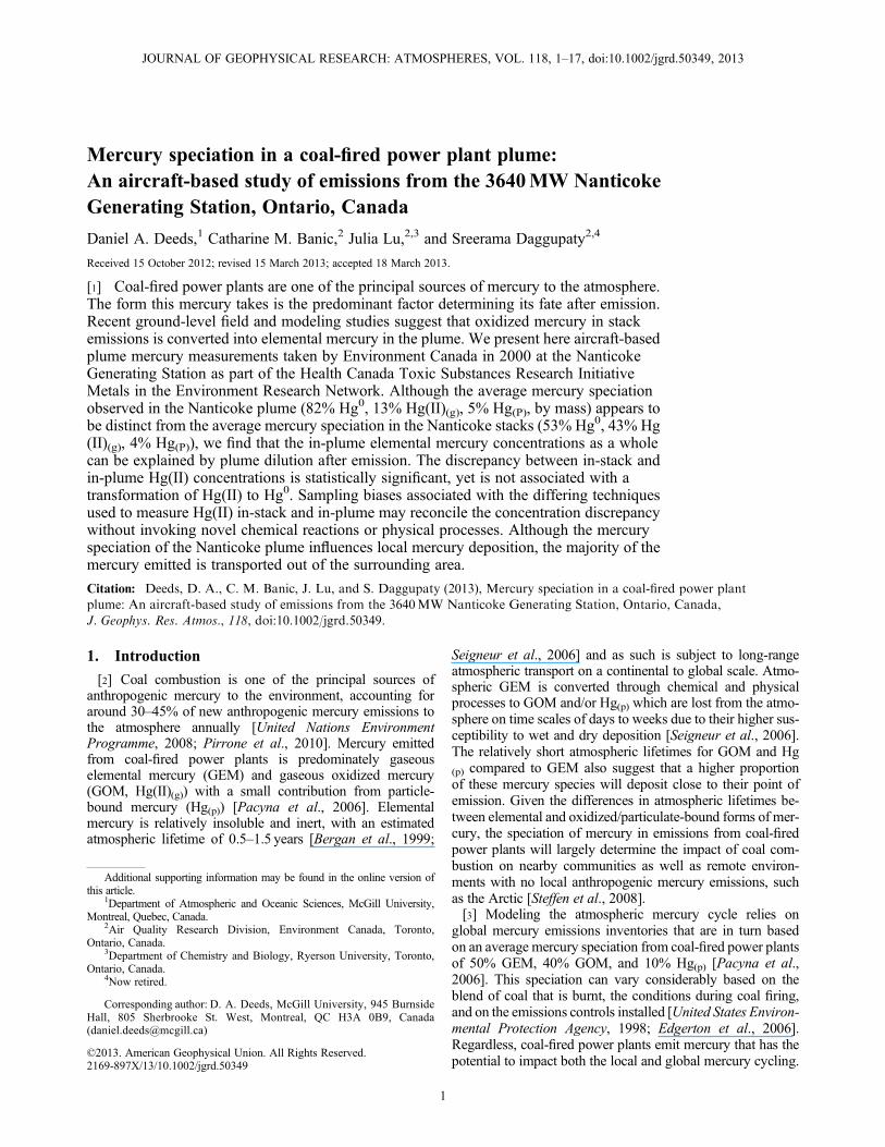
Figure 1. Amap of relative locations of potential sources ofmercury to the regional atmosphere surrounding the NanticokeGenerating Station. Sources of mercury not shown on this mapare the emissions from coal-fired power plants in the OhioRiver Valley, to the south-southwest of this map, as well asthe Imperial Oil refinery and U.S. Steel Works in the immedi-ate proximity of the NGS (see Figure 2).

DEEDS ET AL.: MERCURY IN A COAL-FIRED PLANT PLUME

2

[National Pollution Release Inventory (NPRI), 2000]. Forreference, the Imperial Oil refinery and U.S. Steel Worksnear Nanticoke reported year 2000 mercury emissions of0.95 and 21.5 kg, respectively. Three steel works located inHamilton, to the northeast of Nanticoke, reported combinedemissions of 108 kg Hg in 2000 [NPRI, 2000]. More remoteemitters such as those found in the Ohio River Valley mayalso significantly impact the regional background of atmo-spheric mercury at the study site.[9] The Ontario Power Generation occasionally collects

triplicate mercury speciation measurements in Nanticokeflue gases using the Ontario Hydro Method (OHM). Theclosest three OHM measurements in time to this study weretaken in 1999 in flue gases downstream of the electrostaticprecipitator in Unit 6. The average proportions of mercuryspecies observed were 53% Hg0, 43% Hg(II) and 4% Hg(P)by mass [Lyng et al., 2005], values which are very similarto the average mercury partitioning for North Americancoal-fired plant emissions mentioned above [Pacyna et al.,2006]. Follow-up measurements in 2004 on Unit 6 witha slightly different coal blend (32:68 bituminous:PRB)were consistent with the 1999 OHM speciation measure-ments, with an average mercury proportioning of51:47:2 Hg0:Hg(II):Hg(P), suggesting that the mercury spe-ciation of Nanticoke emissions may be relatively consistentover time. Although limited in number, triplicate mercuryspeciation measurements from other units at Nanticokeshow higher proportions of particulate mercury and lowerproportions of elemental mercury, with averages of36:40:24 and 37:50:13 Hg0:Hg(II):Hg(P) in flue gases fromUnit 2 in 1993 and Unit 3 in 2004, respectively. The extentto which emissions from Units 2, 3, and 6 reflect total emis-sions from the Nanticoke GS is uncertain.

3. Campaign Summary

[10] A description of the TSRI MITE-RN plume campaigncan be found in Banic et al. [2006]; we present here only

those details pertinent to the mercury analyses of theNanticoke plume.[11] During the campaign, 13 flights were made into the

Nanticoke plume between 17 and 28 January 2000, and 12flights were made between 12 and 21 September 2000.GEM measurements are available for 27–28 January and12–21 September, while GOM and Hg(P) measurementswere collected throughout all flights. The duration of eachflight was approximately 2 h. The Nanticoke plume wassampled up to 40 km downwind to study plume ages of upto 1–2 h, in a variety of meteorological conditions, includingsummer and winter, day and night, light to strong winds, andwell-mixed to stable boundary layers. Plumes were trackedusing wind measurement systems developed over the pasttwo decades for this aircraft.[12] A typical flight began with a vertical sampling of the

ambient air upwind of the Nanticoke plume. The aircraftwould then track the plume out to 30 km, followed by verti-cal profiles and horizontal passes of the plume at ranges of20 and 10 km, finishing with a run up the plume to within2 km of the stack. At average winds of 10m s�1, thesedistances correspond to plume aging times of roughly 45,30, 15, and 3min, respectively. Each plume pass was pre-ceded and followed by measurements out past the edges ofthe plume to best characterize the ambient environmentsurrounding the plume. This characterization of the ambientair is critical because of the large dilution of the plume byambient air after emission. The plume was identified bysharp increases in particle and sulfur dioxide concentration,as discussed in section 4.2. The aircraft typically spentbetween 30 and 90 s in plume during a horizontal plumepass. Flights spanned altitudes from 30m above ground toseveral kilometers above ground, depending on the heightof the top of the plume in each flight. Examples of typicalflight tracks are shown in Figure 2.[13] The Twin Otter was equipped with a variety of 1Hz

resolution meteorological instrumentation including tempera-ture, dew point, and vertical and horizontal winds [Banicet al., 2006], as well as instrumentation to measure particle

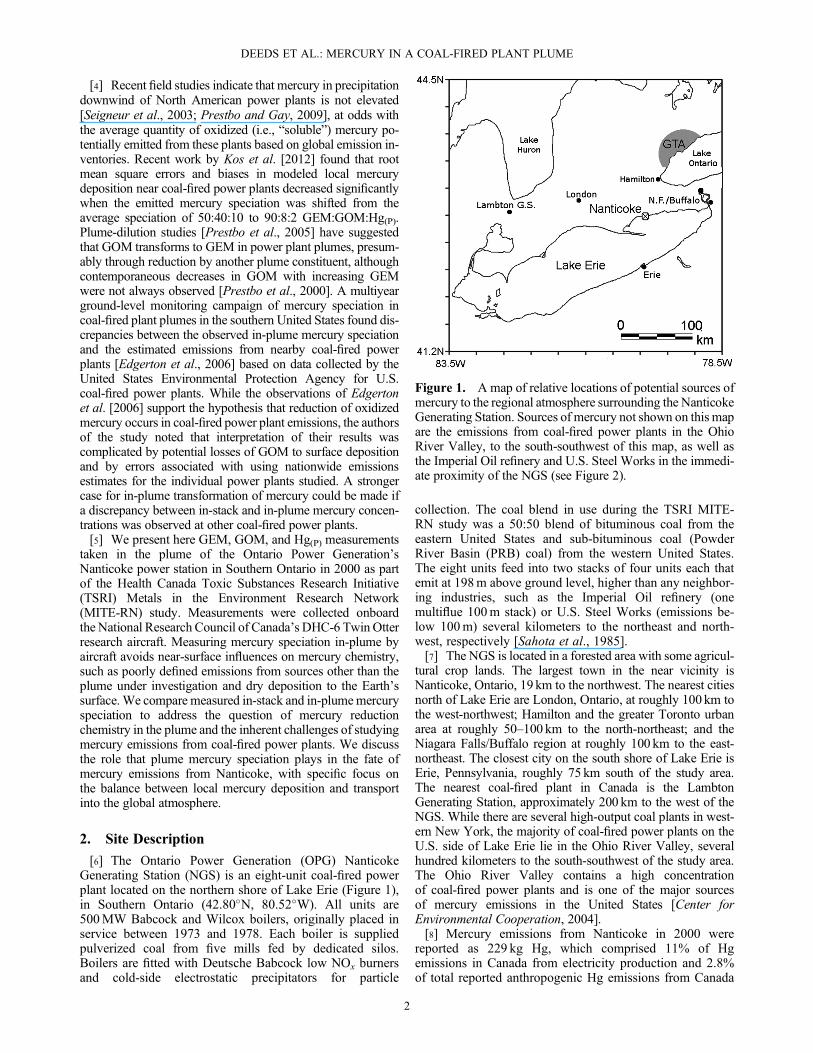
Figure 2. Flight plan for (left) 12 and (right) 20 September 2000, with locations highlighted black where theplume was identified based on particle number concentration and CO2, respectively. Note that longitude ispresented here in degrees E. The Nanticoke Generating Station (square), Imperial Oil refinery (circle), U.S.Steel Stelco steel works (triangle), and airfield (diamond) are shown. The approximate location of the northshore of Lake Erie is indicated by dashed lines. The histogram in the upper left-hand corner of each plotindicates that the wind was predominately from the west-southwest, in accordance with the direction of plumetravel. The plume is relatively coherent with sharp borders and is detected out to the furthest distance traveledfrom the NGS.

DEEDS ET AL.: MERCURY IN A COAL-FIRED PLANT PLUME

3

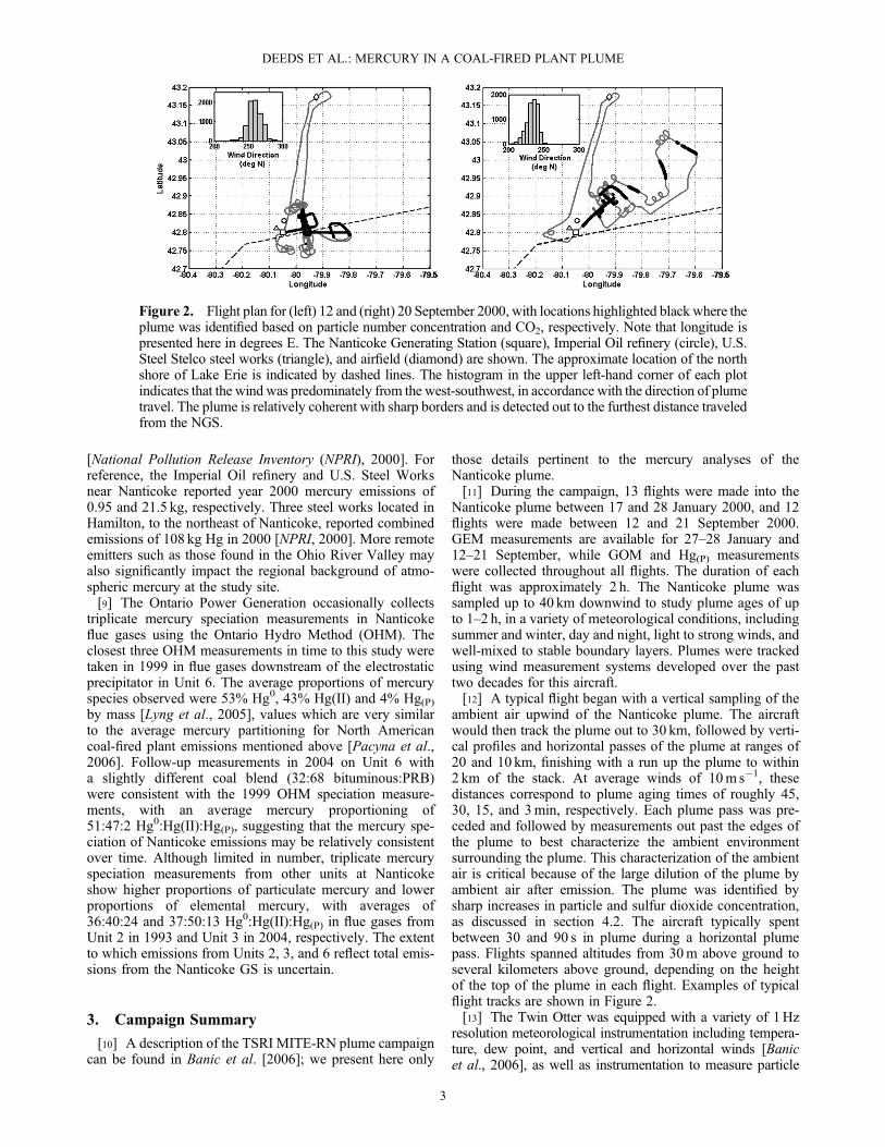
concentration and size distribution and a variety ofatmospheric trace species. Of direct relevance to this studyare the instruments detailed in Table 1.[14] The aircraft was also equipped with a 0.5m3 collapsible

Teflon bag (the “Big Bag Sampler” or “BBS”). The bag wasfilled by air flowing through a forward facing inlet (8 cm by8 cm) with electronically controlled inlet and outlet valves.The BBS is capable of being flushed and filled with outsideair in around 2 s, which allows instruments to sample plumeair for longer lengths of time than the aircraft speed wouldnormally permit during one plume pass. At times throughoutthe campaign, the particulate number concentration, elementalmercury, and SO2 analyzers drew air samples from the BBSfor comparison to the external “plume-average” analyses.[15] In addition to the aircraft instrumentation mentioned

above, a mobile field laboratory was installed several kilome-ters to the west of Nanticoke at Simcoe, Ontario (42.83�N,80.30�W). The field site included a Tekran 2537A AutomatedMercury Monitor for GEM measurement, KCl denuders forGOM sampling, and particle filters for Hg(P) sampling. Thesame manual methods for GOM and Hg(P) analyses were usedat the ground site and on the aircraft. At the ground site, alldenuders and filters were kept in an insulated box at 50�Cduring sampling. Samples were drawn from a height of3.7m above ground level and, based on results of concurrentmeasurements of SO2 and particle number concentration,collected air that was consistently free of the Nanticoke plume.[16] Gaseous elemental mercury measurements were

collected in-flight using a Tekran 2537A. The Tekran 2537Aanalyzer was calibrated using an internal permeation standard;manual injections of mercury-saturated air in-flight throughthe sampling line were periodically performed to assuresample integrity under the harsh sampling conditions. Uncer-tainties for GEM measurement are �10%, based on compari-son of duplicate measurements in the laboratory.[17] Gaseous oxidized mercury was collected on the aircraft

from plume air (winter and summer) and ambient air (summeronly) onto KCl-coated denuders [Landis et al., 2002], with thedenuder sampling ambient conditions drawing air before andafter plume passes. The denuders were mounted on the outside

of the aircraft forward of the propeller line with a 4 cm long,1 cm diameter, curved inlet facing the rear at approximately30 cm from the aircraft skin. The denuders were enclosed ina Teflon case and heated by an air flow from the interior ofthe aircraft. KCl denuders were analyzed at the Simcoe groundstation by decomposition of collected mercury to Hg0 at550�C under a 1.5 Lmin�1 zero-air flow into the Tekran2537A analyzer. The total quantity of mercury collected asGOM, in picograms Hg, was then converted into a corre-sponding GOM concentration (in pgm�3) using the integratedflow of air passed through the denuder in-flight. Given the ex-tremely low concentrations of GOM in air (on the order of10�12 g/m3), only one in-plume sample was collected for eachflight to maximize the quantity of analyte collected. Individualdenuders were tested in the laboratory and were found to haverecovery efficiencies for HgCl2(g) emitted from a diffusionsource (a commonly used GOM proxy) in the range of 70–95%. Recent work by Lyman et al. [2010] indicates that inthe presence of ozone, KCl denuders may undersampleGOM by roughly 20%; the ultrahigh purity nitrogen used asa carrier gas for HgCl2 was ozone free and thus was not re-sponsible for the varying GOM recoveries observed. The un-certainty for GOM measurement is estimated at �40%.[18] In contrast to GEM and GOM, particulate mercury

samples were collected only from the BBS. One filter wascollected for each flight, with air drawn from multiple BigBags filled in the core of the plume. As such, particulate Hgdata represent an average of discrete plume sampling atvarious distances from the source of emission. An aircraftstudy at a copper smelter in Rouyn Noranda, Quebec, usingthe BBS found no systematic difference in dilution-correctedexternal-air and BBS concentrations of particulate As, Cd,Cu, Ni, Pb, Se, and Zn [Wong et al., 2006]. We infer fromthe particulate metal data shown in Wong et al. [2006] thatthe BBS provides a reliable measurement of particulatemercury concentrations as well. At the Simcoe ground station,particulate mercury on sample filters was decomposed toelemental mercury at 900�C under a 1.5 Lmin�1 zero airstream for quantification with the on-site Tekran 2537Aanalyzer. Similar to GOM, total particulate mercury as Hg0

Table 1. Twin Otter Microphysical and Chemical Instrumentation

Parameter Instrument Details Method Installation

Number concentration of particles TSI 7610 >15 nm diameter particles1Hz measurement

Growth to droplets followedby light scattering

Forward facing stainless steelsample inlet

Sulfur dioxide TECO analyzer 1Hz measurement Pulsed UV fluorescence Rear-facing Teflon inlet linemounted 20 cm from aircraftskin drawing air through aTeflon filter

Carbon dioxide LICOR 6262 analyzer 1Hz measurement IR absorption Installed in nose of aircraft forSeptember flights only

Gaseous elemental mercury (GEM) Tekran 2537 analyzer Sampling time of 2.5min Atomic fluorescencespectroscopy

Rear-facing Teflon inlet linemounted 20 cm from aircraftskin drawing air through twoTeflon filters at inlet andinstrument

Gaseous oxidized mercury (GOM) Quartz annularKCl-coated denuder

Kept at ambient Tinlet impactor10 Lmin�1 flow

One in-plume and oneout-of-plume per flight

Roof of the aircraft forward ofthe prop line, denuder inletrear-facing mounted 30 cmfrom aircraft skin

Particulate-associated Hg Pall Flex25-mm quartz filters

At aircraft T10 Lmin�1 flow

One per flight Drawn from Big Bag

DEEDS ET AL.: MERCURY IN A COAL-FIRED PLANT PLUME

4

was converted to a Hg(P) concentration using the integratedflow through the filter in-flight. Ambient air was not sampledfor Hg(p) in flight.[19] The Ontario Power Generation performs a series of

quality control tests on their OHM sampling train prior touse to ensure that their measurements accurately reflect in-stack mercury speciation. Impingers in the sampling train areanalyzed individually to verify mercury collection efficiencies;typically 90% or greater of incoming oxidized and elementalmercury was trapped in the first KCl or KMnO4 impinger,respectively. Recovery efficiencies of each denuder in thesampling train are determined using spiked samples ofmercury and in 1999 were 96% or higher.

4. Results and Discussion

[20] The quality-controlled GEM, GOM, and Hg(p) datacan be found in the supporting information. We present herethe summary and treatment of data pertinent to the discus-sion. All mercury concentrations are presented in units ofmass per standard cubic meter (i.e., at 0�C and 1 atm).

4.1. GEM Correction for Ambient Pressure

[21] During aircraft GEM analyses, the detection cell of theTekran 2537A unit was at reduced pressure as the cell ventsdirectly to the ambient atmosphere of the aircraft which wasnot pressurized. The mass flow of the argon carrier gas enter-ing the detector is constant, resulting in increased volumetricflow and a reduced residence time for mercury in the detectioncell at lower pressures [Ebinghaus and Slemr, 2000]. Thedirect readings from the Tekran analyzer in-flight are thusexpected to be biased low compared to comparable ground-level measurements. Banic et al. [2003] empirically deter-mined the pressure dependency of the Tekran analyzer usedin this study and found that the measured GEM concentration(“GEMmeas” in ngm�3) could be pressure corrected (to“GEMpc” in ngm�3) using the following relationship:

GEMpc ¼ GEMmeas

0:765� Pdð Þ þ 0:25½ � (1)

where Pd is the pressure at the detector cell outlet (expressedin atm). At the relatively low altitudes studied during theNanticoke campaign, this correction typically resulted inadjustments of <5% to measured GEM concentrations. Nopressure correction is necessary for GOM and Hg(P)concentrations, as these measurements were performed postflight at ground level.

4.2. Plume Identification

[22] To determine the concentration of elemental, oxidized,and particulate mercury in the Nanticoke plume, collected datamust be separated into time periods of ambient air or plume airsampling. The Nanticoke plume could be distinguished in realtime from the surrounding ambient air by measurement ofconstituents elevated in the plume with fast-response instru-ments, such as particle number concentration or relative CO2

concentration. For most flights, CO2 concentrations were usedto identify the Nanticoke plume; for flights when CO2 was notavailable, the plume was identified by enhanced particulateconcentration. The threshold for detection of the plume wastaken as the average of ambient concentrations prior to andafter each plume pass (typically two to five measurements in

total) plus 2 times the standard deviation of this mean ambientCO2 concentration. Plumes identified by CO2 data were veri-fied using a combination of SO2 concentrations, particulateconcentrations, and/or wind direction as well as the locationof the aircraft with respect to the stacks. For example, theplume identification for 12 and 20 September is shown inFigure 2. During the January flights and early flights inSeptember, carbon dioxide data were unavailable, and theplume was identified using particulate concentrations (particlediameter >15 nm). An example of the particulate time series,including BBS air analyses, during a flight can be found inFigure 3 of Banic et al. [2006]. Plume identification by partic-ulates was complicated by the presence of nearby particulatesources, in particular the U.S. Steel Lake Erie Works to theimmediate northwest, but was still possible through the useof the supporting information mentioned above.

4.3. Ambient Mercury Concentrations

4.3.1. Gaseous Elemental Mercury[23] Gaseous elemental mercury concentrations in the ambi-

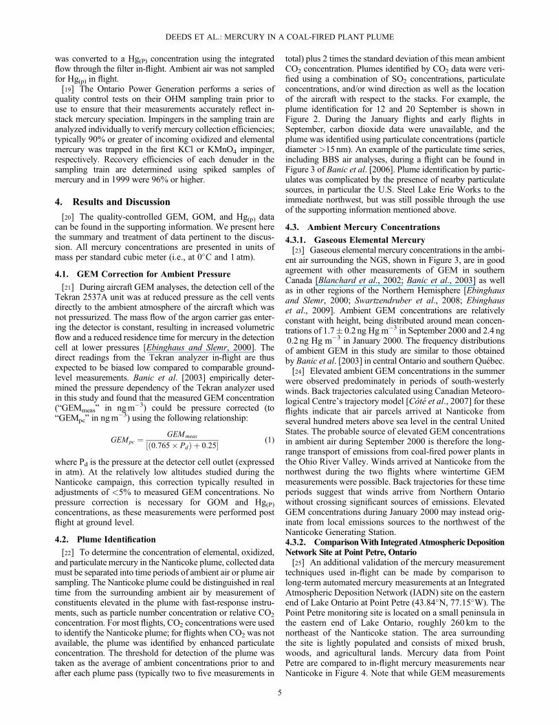
ent air surrounding the NGS, shown in Figure 3, are in goodagreement with other measurements of GEM in southernCanada [Blanchard et al., 2002; Banic et al., 2003] as wellas in other regions of the Northern Hemisphere [Ebinghausand Slemr, 2000; Swartzendruber et al., 2008; Ebinghauset al., 2009]. Ambient GEM concentrations are relativelyconstant with height, being distributed around mean concen-trations of 1.7� 0.2 ng Hg m�3 in September 2000 and 2.4 ng0.2 ng Hg m�3 in January 2000. The frequency distributionsof ambient GEM in this study are similar to those obtainedby Banic et al. [2003] in central Ontario and southern Québec.[24] Elevated ambient GEM concentrations in the summer

were observed predominately in periods of south-westerlywinds. Back trajectories calculated using Canadian Meteoro-logical Centre’s trajectory model [Côté et al., 2007] for theseflights indicate that air parcels arrived at Nanticoke fromseveral hundred meters above sea level in the central UnitedStates. The probable source of elevated GEM concentrationsin ambient air during September 2000 is therefore the long-range transport of emissions from coal-fired power plants inthe Ohio River Valley. Winds arrived at Nanticoke from thenorthwest during the two flights where wintertime GEMmeasurements were possible. Back trajectories for these timeperiods suggest that winds arrive from Northern Ontariowithout crossing significant sources of emissions. ElevatedGEM concentrations during January 2000 may instead orig-inate from local emissions sources to the northwest of theNanticoke Generating Station.4.3.2. ComparisonWith IntegratedAtmosphericDepositionNetwork Site at Point Petre, Ontario[25] An additional validation of the mercury measurement

techniques used in-flight can be made by comparison tolong-term automated mercury measurements at an IntegratedAtmospheric Deposition Network (IADN) site on the easternend of Lake Ontario at Point Petre (43.84�N, 77.15�W). ThePoint Petre monitoring site is located on a small peninsula inthe eastern end of Lake Ontario, roughly 260 km to thenortheast of the Nanticoke station. The area surroundingthe site is lightly populated and consists of mixed brush,woods, and agricultural lands. Mercury data from PointPetre are compared to in-flight mercury measurements nearNanticoke in Figure 4. Note that while GEM measurements

DEEDS ET AL.: MERCURY IN A COAL-FIRED PLANT PLUME

5

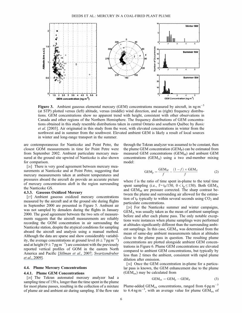
are contemporaneous for Nanticoke and Point Petre, theclosest GOM measurements in time for Point Petre werefrom September 2002. Ambient particulate mercury mea-sured at the ground site upwind of Nanticoke is also shownfor comparison.[26] There is very good agreement between mercury mea-

surements at Nanticoke and at Point Petre, suggesting thatmercury measurements taken at ambient temperatures andpressures aboard the aircraft do provide an accurate pictureof mercury concentrations aloft in the region surroundingthe Nanticoke GS.4.3.3. Gaseous Oxidized Mercury[27] Ambient gaseous oxidized mercury concentrations

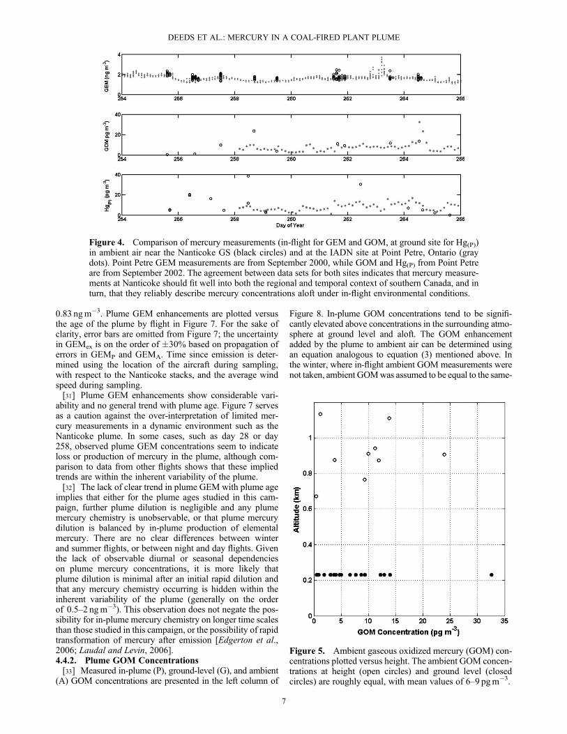
measured by the aircraft and at the ground site during flightsin September 2000 are presented in Figure 5. Ambient airwas not sampled by denuders during the flights in January2000. The good agreement between the two sets of measure-ments suggests that the aircraft measurements are reliablyrecording the GOM concentration in air surrounding theNanticoke station, despite the atypical conditions for samplingaboard the aircraft and analysis using a manual method.Although the data are sparse and show considerably variabil-ity, the average concentrations at ground level (6� 7 pgm�3)and at height (9� 7 pgm�3) are consistent with the previouslyreported vertical profiles of GOM in the eastern NorthAmerica and Pacific [Sillman et al., 2007; Swartzendruberet al., 2009].

4.4. Plume Mercury Concentrations

4.4.1. Plume GEM Concentrations[28] The Tekran automated mercury analyzer had a

sampling time of 150 s, longer than the time spent in the plumefor most plume passes, resulting in the collection of a mixtureof plume air and ambient air during sampling. If the flow rate

through the Tekran analyzer was assumed to be constant, thenthe plume GEM concentration (GEMP) can be estimated frommeasured GEM concentrations (GEMM) and ambient GEMconcentrations (GEMA) using a two end-member mixingmodel:

GEMp ¼ GEMM

f� 1� fð Þ � GEMA

f(2)

where f is the ratio of time spent in-plume to the total timespent sampling (i.e., f = tP/150, 0< tp ≤ 150). Both GEMA

and GEMM are pressure corrected. The sharp contrast be-tween the plume and surrounding air allowed for the estima-tion of tP typically to within several seconds using CO2 andparticulate concentrations.[29] For the Nanticoke summer and winter campaigns,

GEMA was usually taken as the mean of ambient samplingsbefore and after each plume pass. The only notable excep-tions were instances when plume samplings were performedat altitudes significantly different than the surrounding ambi-ent samplings. In this case, GEMA was determined from themean of same-day ambient measurements taken at altitudesclose to the plume pass in question. The resulting plumeconcentrations are plotted alongside ambient GEM concen-trations in Figure 6. Plume GEM concentrations are elevatedcompared to ambient GEM concentrations, but typically byless than 2 times the ambient, consistent with rapid plumedilution after emission.[30] Once the GEM concentration in-plume for a particu-

lar pass is known, the GEM enhancement due to the plume(GEMex) may be calculated from

GEMex ¼ GEMp � GEMA (3)

Plume-added GEMex concentrations, ranged from 6 pgm�3

to 6.4 ngm�3, with an average value for plume GEMex of

Figure 3. Ambient gaseous elemental mercury (GEM) concentrations measured by aircraft, in ngm�3

(at STP) plotted versus (left) altitude, versus (middle) wind direction, and as (right) frequency distribu-tions. GEM concentrations show no apparent trend with height, consistent with other observations inCanada and other regions of the Northern Hemisphere. The frequency distributions of GEM concentra-tions obtained in this study resemble distributions taken in central Ontario and southern Québec by Banicet al. [2003]. Air originated in this study from the west, with elevated concentrations in winter from thenorthwest and in summer from the southwest. Elevated ambient GEM is likely a result of local sourcesin winter and long-range transport in the summer.

DEEDS ET AL.: MERCURY IN A COAL-FIRED PLANT PLUME

6

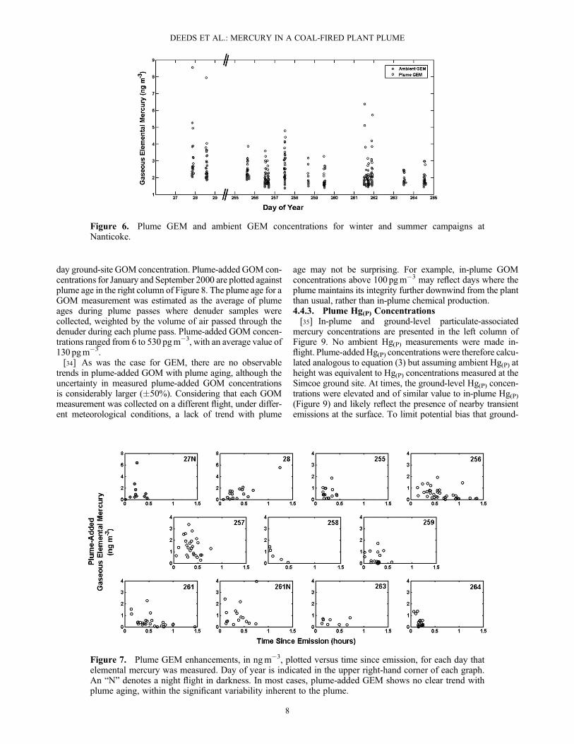
0.83 ngm�3. Plume GEM enhancements are plotted versusthe age of the plume by flight in Figure 7. For the sake ofclarity, error bars are omitted from Figure 7; the uncertaintyin GEMex is on the order of �30% based on propagation oferrors in GEMP and GEMA. Time since emission is deter-mined using the location of the aircraft during sampling,with respect to the Nanticoke stacks, and the average windspeed during sampling.[31] Plume GEM enhancements show considerable vari-

ability and no general trend with plume age. Figure 7 servesas a caution against the over-interpretation of limited mer-cury measurements in a dynamic environment such as theNanticoke plume. In some cases, such as day 28 or day258, observed plume GEM concentrations seem to indicateloss or production of mercury in the plume, although com-parison to data from other flights shows that these impliedtrends are within the inherent variability of the plume.[32] The lack of clear trend in plume GEM with plume age

implies that either for the plume ages studied in this cam-paign, further plume dilution is negligible and any plumemercury chemistry is unobservable, or that plume mercurydilution is balanced by in-plume production of elementalmercury. There are no clear differences between winterand summer flights, or between night and day flights. Giventhe lack of observable diurnal or seasonal dependencieson plume mercury concentrations, it is more likely thatplume dilution is minimal after an initial rapid dilution andthat any mercury chemistry occurring is hidden within theinherent variability of the plume (generally on the orderof 0.5–2 ngm�3). This observation does not negate the pos-sibility for in-plume mercury chemistry on longer time scalesthan those studied in this campaign, or the possibility of rapidtransformation of mercury after emission [Edgerton et al.,2006; Laudal and Levin, 2006].4.4.2. Plume GOM Concentrations[33] Measured in-plume (P), ground-level (G), and ambient

(A) GOM concentrations are presented in the left column of

Figure 8. In-plume GOM concentrations tend to be signifi-cantly elevated above concentrations in the surrounding atmo-sphere at ground level and aloft. The GOM enhancementadded by the plume to ambient air can be determined usingan equation analogous to equation (3) mentioned above. Inthe winter, where in-flight ambient GOM measurements werenot taken, ambient GOMwas assumed to be equal to the same-

Figure 4. Comparison of mercury measurements (in-flight for GEM and GOM, at ground site for Hg(P))in ambient air near the Nanticoke GS (black circles) and at the IADN site at Point Petre, Ontario (graydots). Point Petre GEM measurements are from September 2000, while GOM and Hg(P) from Point Petreare from September 2002. The agreement between data sets for both sites indicates that mercury measure-ments at Nanticoke should fit well into both the regional and temporal context of southern Canada, and inturn, that they reliably describe mercury concentrations aloft under in-flight environmental conditions.

Figure 5. Ambient gaseous oxidized mercury (GOM) con-centrations plotted versus height. The ambient GOM concen-trations at height (open circles) and ground level (closedcircles) are roughly equal, with mean values of 6–9 pgm�3.

DEEDS ET AL.: MERCURY IN A COAL-FIRED PLANT PLUME

7

day ground-site GOM concentration. Plume-added GOM con-centrations for January and September 2000 are plotted againstplume age in the right column of Figure 8. The plume age for aGOM measurement was estimated as the average of plumeages during plume passes where denuder samples werecollected, weighted by the volume of air passed through thedenuder during each plume pass. Plume-added GOM concen-trations ranged from 6 to 530 pgm�3, with an average value of130 pgm�3.[34] As was the case for GEM, there are no observable

trends in plume-added GOM with plume aging, although theuncertainty in measured plume-added GOM concentrationsis considerably larger (�50%). Considering that each GOMmeasurement was collected on a different flight, under differ-ent meteorological conditions, a lack of trend with plume

age may not be surprising. For example, in-plume GOMconcentrations above 100 pgm�3 may reflect days where theplume maintains its integrity further downwind from the plantthan usual, rather than in-plume chemical production.4.4.3. Plume Hg(P) Concentrations[35] In-plume and ground-level particulate-associated

mercury concentrations are presented in the left column ofFigure 9. No ambient Hg(P) measurements were made in-flight. Plume-added Hg(P) concentrations were therefore calcu-lated analogous to equation (3) but assuming ambient Hg(P) atheight was equivalent to Hg(P) concentrations measured at theSimcoe ground site. At times, the ground-level Hg(P) concen-trations were elevated and of similar value to in-plume Hg(P)(Figure 9) and likely reflect the presence of nearby transientemissions at the surface. To limit potential bias that ground-

Figure 6. Plume GEM and ambient GEM concentrations for winter and summer campaigns atNanticoke.

Figure 7. Plume GEM enhancements, in ngm�3, plotted versus time since emission, for each day thatelemental mercury was measured. Day of year is indicated in the upper right-hand corner of each graph.An “N” denotes a night flight in darkness. In most cases, plume-added GEM shows no clear trend withplume aging, within the significant variability inherent to the plume.

DEEDS ET AL.: MERCURY IN A COAL-FIRED PLANT PLUME

8

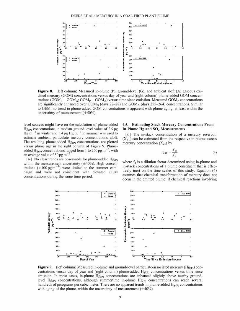
level sources might have on the calculation of plume-addedHg(P) concentrations, a median ground-level value of 2.9 pgHg m�3 in winter and 5.4 pg Hg m�3 in summer was used toestimate ambient particulate mercury concentrations aloft.The resulting plume-added Hg(P) concentrations are plottedversus plume age in the right column of Figure 9. Plume-added Hg(P) concentrations ranged from 1 to 250 pgm�3, withan average value of 50 pgm�3.[36] No clear trends are observable for plume-added Hg(P)

within the measurement uncertainty (�40%). High concen-trations (>100 pgm�3) were limited to the summer cam-paign and were not coincident with elevated GOMconcentrations during the same time period.

4.5. Estimating Stack Mercury Concentrations FromIn-Plume Hg and SO2 Measurements

[37] The in-stack concentration of a mercury reservoir(XST) can be estimated from the respective in-plume excessmercury concentration (Xex) by

X ST ¼ X ex

f d(4)

where fd is a dilution factor determined using in-plume andin-stack concentrations of a plume constituent that is effec-tively inert on the time scales of this study. Equation (4)assumes that chemical transformation of mercury does notoccur in the emitted plume; if chemical reactions involving

Figure 8. (left column) Measured in-plume (P), ground-level (G), and ambient aloft (A) gaseous oxi-dized mercury (GOM) concentrations versus day of year and (right column) plume-added GOM concen-trations (GOMP�GOMG; GOMP�GOMA) versus time since emission. Measured GOMP concentrationsare significantly enhanced over GOMG (days 22–28) and GOMA (days 255–264) concentrations. Similarto GEM, no trend in plume-added GOM concentrations is apparent with plume aging, at least within theuncertainty of measurement (�50%).

Figure 9. (left column) Measured in-plume and ground-level particulate-associated mercury (Hg(P)) con-centrations versus day of year and (right column) plume-added Hg(P) concentrations versus time sinceemission. In most cases, in-plume Hg(P) concentrations are enhanced slightly above nearby ground-level Hg(P) concentrations, although summertime in-plume Hg(P) concentrations can reach severalhundreds of picograms per cubic meter. There are no apparent trends in plume-added Hg(P) concentrationswith aging of the plume, within the uncertainty of measurement (�40%).

DEEDS ET AL.: MERCURY IN A COAL-FIRED PLANT PLUME

9

mercury do occur, then the XST estimated using equation (4)may significantly differ from measured in-stack mercuryconcentrations.[38] We estimate plume dilution using plume and stack

sulfur dioxide concentrations, given the comparatively largeconcentrations emitted by the NGS (~420 ppm SO2) and therelatively slow rate at which SO2 is lost from the Nanticokeplume, ~1–4% per hour [Anlauf et al., 1982]. Stack SO2

concentrations with a time resolution of 1min measured usinga continuous emissions monitoring system for January andSeptember 2000 were provided by Ontario Power Generation.Plume SO2 measurements could be paired with stack SO2

concentrations based on estimated plume ages and the timeof sampling. However, due to the strong gradient in SO2 onvery short time scales, the aircraft-measured plume SO2

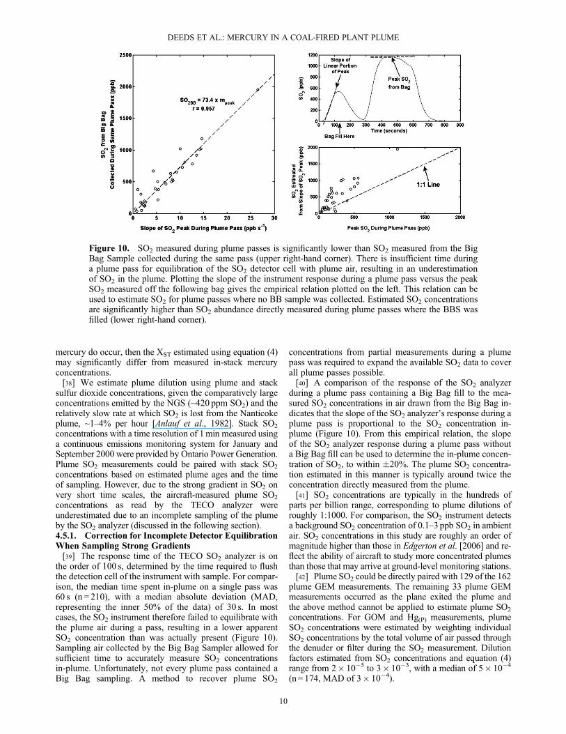
concentrations as read by the TECO analyzer wereunderestimated due to an incomplete sampling of the plumeby the SO2 analyzer (discussed in the following section).4.5.1. Correction for Incomplete Detector EquilibrationWhen Sampling Strong Gradients[39] The response time of the TECO SO2 analyzer is on

the order of 100 s, determined by the time required to flushthe detection cell of the instrument with sample. For compar-ison, the median time spent in-plume on a single pass was60 s (n = 210), with a median absolute deviation (MAD,representing the inner 50% of the data) of 30 s. In mostcases, the SO2 instrument therefore failed to equilibrate withthe plume air during a pass, resulting in a lower apparentSO2 concentration than was actually present (Figure 10).Sampling air collected by the Big Bag Sampler allowed forsufficient time to accurately measure SO2 concentrationsin-plume. Unfortunately, not every plume pass contained aBig Bag sampling. A method to recover plume SO2

concentrations from partial measurements during a plumepass was required to expand the available SO2 data to coverall plume passes possible.[40] A comparison of the response of the SO2 analyzer

during a plume pass containing a Big Bag fill to the mea-sured SO2 concentrations in air drawn from the Big Bag in-dicates that the slope of the SO2 analyzer’s response during aplume pass is proportional to the SO2 concentration in-plume (Figure 10). From this empirical relation, the slopeof the SO2 analyzer response during a plume pass withouta Big Bag fill can be used to determine the in-plume concen-tration of SO2, to within �20%. The plume SO2 concentra-tion estimated in this manner is typically around twice theconcentration directly measured from the plume.[41] SO2 concentrations are typically in the hundreds of

parts per billion range, corresponding to plume dilutions ofroughly 1:1000. For comparison, the SO2 instrument detectsa background SO2 concentration of 0.1–3 ppb SO2 in ambientair. SO2 concentrations in this study are roughly an order ofmagnitude higher than those in Edgerton et al. [2006] and re-flect the ability of aircraft to study more concentrated plumesthan those that may arrive at ground-level monitoring stations.[42] Plume SO2 could be directly paired with 129 of the 162

plume GEM measurements. The remaining 33 plume GEMmeasurements occurred as the plane exited the plume andthe above method cannot be applied to estimate plume SO2

concentrations. For GOM and Hg(P) measurements, plumeSO2 concentrations were estimated by weighting individualSO2 concentrations by the total volume of air passed throughthe denuder or filter during the SO2 measurement. Dilutionfactors estimated from SO2 concentrations and equation (4)range from 2� 10�5 to 3� 10�3, with a median of 5� 10�4

(n= 174, MAD of 3� 10�4).

Figure 10. SO2 measured during plume passes is significantly lower than SO2 measured from the BigBag Sample collected during the same pass (upper right-hand corner). There is insufficient time duringa plume pass for equilibration of the SO2 detector cell with plume air, resulting in an underestimationof SO2 in the plume. Plotting the slope of the instrument response during a plume pass versus the peakSO2 measured off the following bag gives the empirical relation plotted on the left. This relation can beused to estimate SO2 for plume passes where no BB sample was collected. Estimated SO2 concentrationsare significantly higher than SO2 abundance directly measured during plume passes where the BBS wasfilled (lower right-hand corner).

DEEDS ET AL.: MERCURY IN A COAL-FIRED PLANT PLUME

10

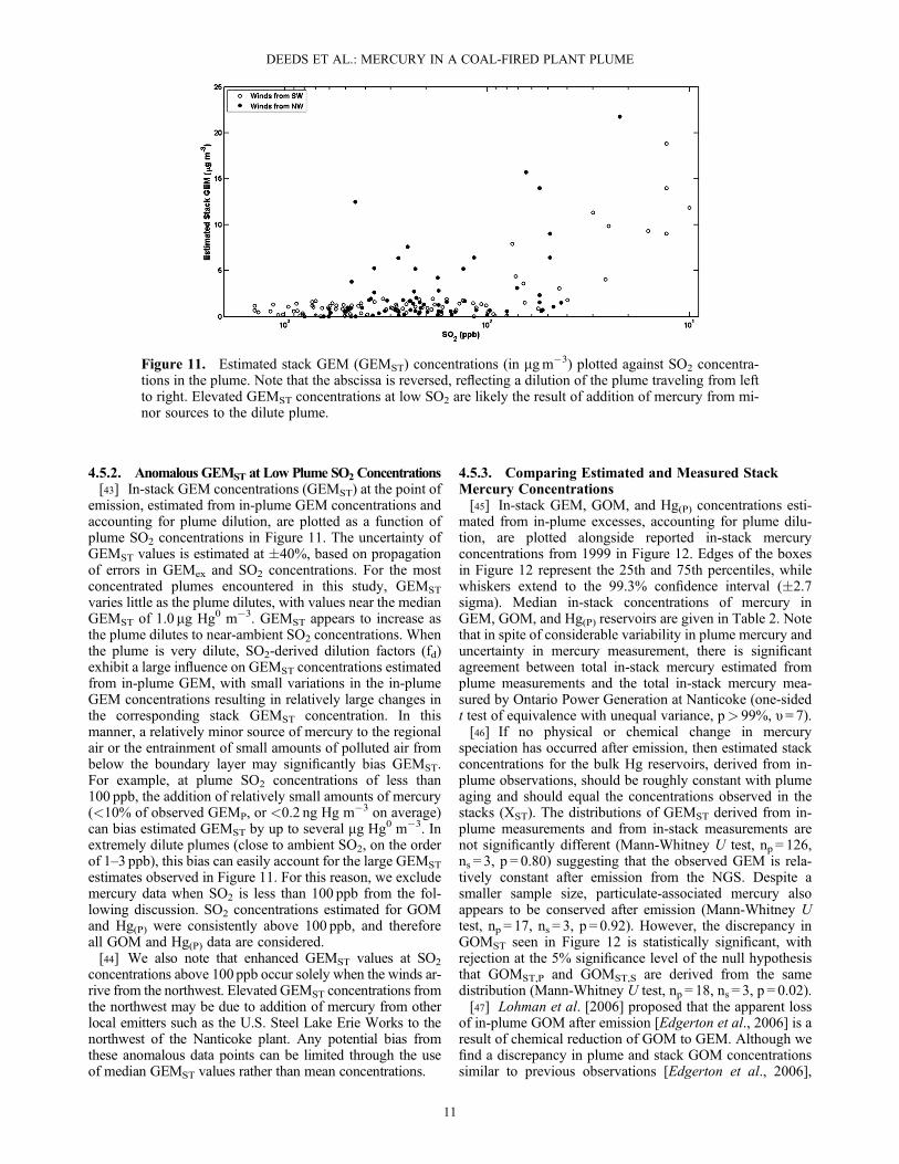
4.5.2. Anomalous GEMST at Low Plume SO2 Concentrations[43] In-stack GEM concentrations (GEMST) at the point of

emission, estimated from in-plume GEM concentrations andaccounting for plume dilution, are plotted as a function ofplume SO2 concentrations in Figure 11. The uncertainty ofGEMST values is estimated at �40%, based on propagationof errors in GEMex and SO2 concentrations. For the mostconcentrated plumes encountered in this study, GEMST

varies little as the plume dilutes, with values near the medianGEMST of 1.0 mg Hg0 m�3. GEMST appears to increase asthe plume dilutes to near-ambient SO2 concentrations. Whenthe plume is very dilute, SO2-derived dilution factors (fd)exhibit a large influence on GEMST concentrations estimatedfrom in-plume GEM, with small variations in the in-plumeGEM concentrations resulting in relatively large changes inthe corresponding stack GEMST concentration. In thismanner, a relatively minor source of mercury to the regionalair or the entrainment of small amounts of polluted air frombelow the boundary layer may significantly bias GEMST.For example, at plume SO2 concentrations of less than100 ppb, the addition of relatively small amounts of mercury(<10% of observed GEMP, or <0.2 ng Hg m�3 on average)can bias estimated GEMST by up to several mg Hg0 m�3. Inextremely dilute plumes (close to ambient SO2, on the orderof 1–3 ppb), this bias can easily account for the large GEMST

estimates observed in Figure 11. For this reason, we excludemercury data when SO2 is less than 100 ppb from the fol-lowing discussion. SO2 concentrations estimated for GOMand Hg(P) were consistently above 100 ppb, and thereforeall GOM and Hg(P) data are considered.[44] We also note that enhanced GEMST values at SO2

concentrations above 100 ppb occur solely when the winds ar-rive from the northwest. Elevated GEMST concentrations fromthe northwest may be due to addition of mercury from otherlocal emitters such as the U.S. Steel Lake Erie Works to thenorthwest of the Nanticoke plant. Any potential bias fromthese anomalous data points can be limited through the useof median GEMST values rather than mean concentrations.

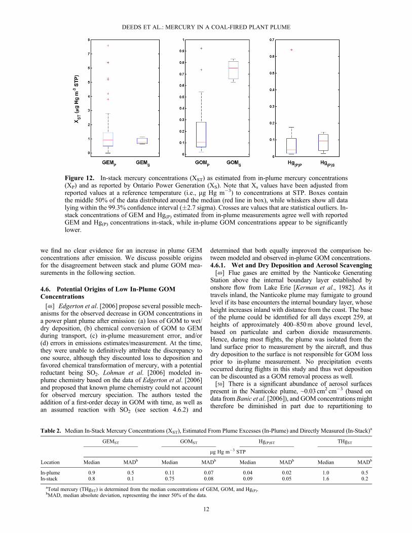
4.5.3. Comparing Estimated and Measured StackMercury Concentrations[45] In-stack GEM, GOM, and Hg(P) concentrations esti-

mated from in-plume excesses, accounting for plume dilu-tion, are plotted alongside reported in-stack mercuryconcentrations from 1999 in Figure 12. Edges of the boxesin Figure 12 represent the 25th and 75th percentiles, whilewhiskers extend to the 99.3% confidence interval (�2.7sigma). Median in-stack concentrations of mercury inGEM, GOM, and Hg(P) reservoirs are given in Table 2. Notethat in spite of considerable variability in plume mercury anduncertainty in mercury measurement, there is significantagreement between total in-stack mercury estimated fromplume measurements and the total in-stack mercury mea-sured by Ontario Power Generation at Nanticoke (one-sidedt test of equivalence with unequal variance, p> 99%, υ= 7).[46] If no physical or chemical change in mercury

speciation has occurred after emission, then estimated stackconcentrations for the bulk Hg reservoirs, derived from in-plume observations, should be roughly constant with plumeaging and should equal the concentrations observed in thestacks (XST). The distributions of GEMST derived from in-plume measurements and from in-stack measurements arenot significantly different (Mann-Whitney U test, np = 126,ns = 3, p = 0.80) suggesting that the observed GEM is rela-tively constant after emission from the NGS. Despite asmaller sample size, particulate-associated mercury alsoappears to be conserved after emission (Mann-Whitney Utest, np = 17, ns = 3, p = 0.92). However, the discrepancy inGOMST seen in Figure 12 is statistically significant, withrejection at the 5% significance level of the null hypothesisthat GOMST,P and GOMST,S are derived from the samedistribution (Mann-Whitney U test, np = 18, ns = 3, p = 0.02).[47] Lohman et al. [2006] proposed that the apparent loss

of in-plume GOM after emission [Edgerton et al., 2006] is aresult of chemical reduction of GOM to GEM. Although wefind a discrepancy in plume and stack GOM concentrationssimilar to previous observations [Edgerton et al., 2006],

Figure 11. Estimated stack GEM (GEMST) concentrations (in mgm�3) plotted against SO2 concentra-tions in the plume. Note that the abscissa is reversed, reflecting a dilution of the plume traveling from leftto right. Elevated GEMST concentrations at low SO2 are likely the result of addition of mercury from mi-nor sources to the dilute plume.

DEEDS ET AL.: MERCURY IN A COAL-FIRED PLANT PLUME

11

we find no clear evidence for an increase in plume GEMconcentrations after emission. We discuss possible originsfor the disagreement between stack and plume GOM mea-surements in the following section.

4.6. Potential Origins of Low In-Plume GOMConcentrations

[48] Edgerton et al. [2006] propose several possible mech-anisms for the observed decrease in GOM concentrations ina power plant plume after emission: (a) loss of GOM to wet/dry deposition, (b) chemical conversion of GOM to GEMduring transport, (c) in-plume measurement error, and/or(d) errors in emissions estimates/measurement. At the time,they were unable to definitively attribute the discrepancy toone source, although they discounted loss to deposition andfavored chemical transformation of mercury, with a potentialreductant being SO2. Lohman et al. [2006] modeled in-plume chemistry based on the data of Edgerton et al. [2006]and proposed that known plume chemistry could not accountfor observed mercury speciation. The authors tested theaddition of a first-order decay in GOM with time, as well asan assumed reaction with SO2 (see section 4.6.2) and

determined that both equally improved the comparison be-tween modeled and observed in-plume GOM concentrations.4.6.1. Wet and Dry Deposition and Aerosol Scavenging[49] Flue gases are emitted by the Nanticoke Generating

Station above the internal boundary layer established byonshore flow from Lake Erie [Kerman et al., 1982]. As ittravels inland, the Nanticoke plume may fumigate to groundlevel if its base encounters the internal boundary layer, whoseheight increases inland with distance from the coast. The baseof the plume could be identified for all days except 259, atheights of approximately 400–850m above ground level,based on particulate and carbon dioxide measurements.Hence, during most flights, the plume was isolated from theland surface prior to measurement by the aircraft, and thusdry deposition to the surface is not responsible for GOM lossprior to in-plume measurement. No precipitation eventsoccurred during flights in this study and thus wet depositioncan be discounted as a GOM removal process as well.[50] There is a significant abundance of aerosol surfaces

present in the Nanticoke plume, ~0.03 cm2 cm�3 (based ondata from Banic et al. [2006]), and GOM concentrations mighttherefore be diminished in part due to repartitioning to

Table 2. Median In-Stack Mercury Concentrations (XST), Estimated From Plume Excesses (In-Plume) and Directly Measured (In-Stack)a

Location

GEMST GOMST Hg(P)ST THgST

mg Hg m�3 STP

Median MADb Median MADb Median MADb Median MADb

In-plume 0.9 0.5 0.11 0.07 0.04 0.02 1.0 0.5In-stack 0.8 0.1 0.75 0.08 0.09 0.05 1.6 0.2

aTotal mercury (THgST) is determined from the median concentrations of GEM, GOM, and Hg(P).bMAD, median absolute deviation, representing the inner 50% of the data.

Figure 12. In-stack mercury concentrations (XST) as estimated from in-plume mercury concentrations(XP) and as reported by Ontario Power Generation (XS). Note that Xs values have been adjusted fromreported values at a reference temperature (i.e., mg Hg m�3) to concentrations at STP. Boxes containthe middle 50% of the data distributed around the median (red line in box), while whiskers show all datalying within the 99.3% confidence interval (�2.7 sigma). Crosses are values that are statistical outliers. In-stack concentrations of GEM and Hg(P) estimated from in-plume measurements agree well with reportedGEM and Hg(P) concentrations in-stack, while in-plume GOM concentrations appear to be significantlylower.

DEEDS ET AL.: MERCURY IN A COAL-FIRED PLANT PLUME

12

particulate mercury. As noted previously, there is no evidence,within the uncertainty of measurement, for an enhancement ofparticulate mercury concentrations with respect to stack emis-sions, suggesting that there is no net transfer of GOM to parti-cle surfaces in the plume.[51] Rutter and Schauer [2007a] found equilibration

between particulate-bound and gas-phase GOM to be veryrapid (on the order of seconds), with equilibrium GOM gas-particle partitioning coefficients of 1–10m3mg�1 for sulfateaerosols. Using a sulfate aerosol concentration of roughly 9mgm�3 for the Nanticoke plume [Anlauf et al., 1982], theabove partitioning coefficient gives an estimated equilibriumHg(p)/GOM ratio of 0.1–1.1 [Rutter and Schauer, 2007a].Winter Hg(P)ST/GOMST ratios in the plume range from 0.03to 0.96. Summertime Hg(P)ST/GOMST ratios in the plumerange from 0.03 to 1.9. Only flights on days 26, 257, 258,and 261 fall outside the expected equilibrium gas-particlepartitioning ratio, with values of 0.03, 1.6, 1.9, and 0.03, re-spectively. GOM and Hg(P) appear to be in equilibrium forthe majority of days studied here, regardless of seasonalityor time of day. We note that this may not preclude GOMto Hg(P) transfer during and directly after emission of theplume, when particle mass concentration would be consider-ably higher, but this transfer may be limited by a reducedGOM uptake at the higher stack temperatures [Rutter andSchauer, 2007b].4.6.2. Chemical Reduction of GOM to GEM[52] Although we find no clear evidence for a transforma-

tion of GOM to GEM in the Nanticoke plume, we may stillconsider whether proposed reductants are capable ofconverting GOM to GEM in-plume after emission.[53] Lohman et al. [2006] proposed that oxidized mercury

was reduced by sulfur dioxide through a three-stepmechanismsuggested by Scott et al. [2003] and based on an IR productstudy of the reaction SO2(g) +HgO(s) [Zacharewksi et al.,1987]. The end-products of the reaction of HgO with SO2were found to be HgS(s), HgSO4(s), and Hg2SO4(s)[Zacharewksi et al., 1987]. In-plume reaction of oxidizedmercury by SO2 would thus convert particulate mercury(HgO(s)) into other forms of particulate mercury (e.g.,HgSO4(s)) and would at most reduce Hg(II) to Hg(I).[54] It may be possible that reduction of GOM occurs in the

aqueous phase, in liquid layers on aerosol surfaces or clouddroplets. Sulfite and HO2 have been proposed as aqueous phasereductants of oxidized mercury [Munthe et al., 1991; Pehkonenand Lin, 1998]. The thermodynamic favorability of mercury re-duction by HO2 has been questioned [Gårdfeldt and Jonsson,2003]. At high SO2 concentrations in the Nanticoke plume(hundreds of parts per billion SO2), Hg(II) will react with sulfiteto form a stable mercury-sulfur complex, Hg SO3ð Þ2�2 [VanLoon et al., 2001]. As the plume dilutes, and sulfite concentra-tions decrease, Hg SO3ð Þ2�2 should dissociate to redox-unstableHg(SO3), which in turn decomposes to Hg0. Van Loon et al.[2001] suggest that elemental mercury produced fromHg(SO3) complexes with SO2(aq) to form Hg � SO2(aq), withan apparent solubility 3 orders of magnitude higher thanHg0 alone [Van Loon et al., 2001]. Reduction of oxidizedmercury in the presence of sulfite may therefore occur in liq-uid layers on aerosols or in liquid water droplets in theNanticoke plume as it dilutes into the regional atmosphere.Given the relatively high solubility of the Hg � SO2(aq)

complex, we suggest that the reduced mercury likely re-mains in the particulate phase, although evaporation of liq-uid layers or droplets might release the Hg0 into the gasphase. We note that if reduction of GOM to Hg � SO2(aq) oc-curs in the Nanticoke plume, then the net transfer of mercurywould be from gaseous oxidized mercury to particulate mer-cury. As we have previously noted, we find no evidence tosupport a net transfer of GOM to Hg(p). Photoreduction ofoxidized mercury is known to occur, with a midday half-life of roughly a month [Lin and Pehkonen, 1999], and islikely not significant on the time scales of this study.4.6.3. Stack and Plume Measurement Uncertainties[55] One significant source of uncertainty is the limited

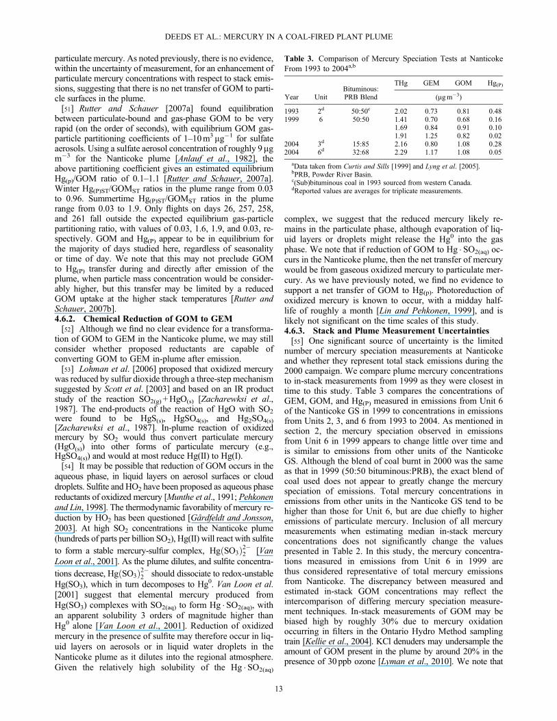
number of mercury speciation measurements at Nanticokeand whether they represent total stack emissions during the2000 campaign. We compare plume mercury concentrationsto in-stack measurements from 1999 as they were closest intime to this study. Table 3 compares the concentrations ofGEM, GOM, and Hg(P) measured in emissions from Unit 6of the Nanticoke GS in 1999 to concentrations in emissionsfrom Units 2, 3, and 6 from 1993 to 2004. As mentioned insection 2, the mercury speciation observed in emissionsfrom Unit 6 in 1999 appears to change little over time andis similar to emissions from other units of the NanticokeGS. Although the blend of coal burnt in 2000 was the sameas that in 1999 (50:50 bituminous:PRB), the exact blend ofcoal used does not appear to greatly change the mercuryspeciation of emissions. Total mercury concentrations inemissions from other units in the Nanticoke GS tend to behigher than those for Unit 6, but are due chiefly to higheremissions of particulate mercury. Inclusion of all mercurymeasurements when estimating median in-stack mercuryconcentrations does not significantly change the valuespresented in Table 2. In this study, the mercury concentra-tions measured in emissions from Unit 6 in 1999 arethus considered representative of total mercury emissionsfrom Nanticoke. The discrepancy between measured andestimated in-stack GOM concentrations may reflect theintercomparison of differing mercury speciation measure-ment techniques. In-stack measurements of GOM may bebiased high by roughly 30% due to mercury oxidationoccurring in filters in the Ontario Hydro Method samplingtrain [Kellie et al., 2004]. KCl denuders may undersample theamount of GOM present in the plume by around 20% in thepresence of 30 ppb ozone [Lyman et al., 2010]. We note that

Table 3. Comparison of Mercury Speciation Tests at NanticokeFrom 1993 to 2004a,b

Year UnitBituminous:PRB Blend

THg GEM GOM Hg(P)

(mgm�3)

1993 2d 50:50c 2.02 0.73 0.81 0.481999 6 50:50 1.41 0.70 0.68 0.16

1.69 0.84 0.91 0.101.91 1.25 0.82 0.02

2004 3d 15:85 2.16 0.80 1.08 0.282004 6d 32:68 2.29 1.17 1.08 0.05

aData taken from Curtis and Sills [1999] and Lyng et al. [2005].bPRB, Powder River Basin.c(Sub)bituminous coal in 1993 sourced from western Canada.dReported values are averages for triplicate measurements.

DEEDS ET AL.: MERCURY IN A COAL-FIRED PLANT PLUME

13

the efficiency of collection and recovery of other GOM speciesthan HgCl2 by denuders used in this study is unknown.[56] If we assume both ambient and plume GOMmeasure-

ments were biased during the 2000 aircraft campaign, thedifference between measured in-stack GOM and estimatedin-stack GOM from plume measurements decreases from0.64 mgm�3 to 0.39 mgm�3. The probability of equivalencebetween bias-corrected measured and estimated stackGOM concentrations remains low (Mann-Whitney U test,n1 = 18, n2 = 3, p = 0.12) but cannot be rejected on a statisti-cal basis. There is thus a small chance that the two data setsare equivalent and that there is no discrepancy in stack andplume-derived GOMST concentrations. Further testing ofexisting methods for measurement of in-stack and in-plumemercury speciation and development of new methods formercury measurement would be a great aid in addressingwhether a discrepancy between stack and plume mercuryspeciation exists.

4.7. Mercury Speciation and The Local and GlobalImpact of the Nanticoke Generating Station

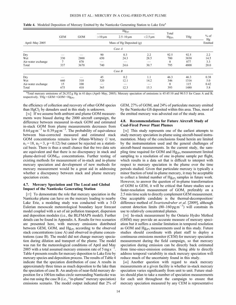
[57] To demonstrate the role that mercury speciation in theNanticoke plume can have on the mercury loading to nearbyLake Erie, a modeling study was conducted with a 3-DEulerian mesoscale meteorological boundary layer forecastmodel coupled with a set of air pollution transport, dispersionand deposition modules (i.e., the BLFMAPS model). Furtherdetails can be found in Appendix A. Results for two scenariosare presented here, with mercury emissions distributedbetween GEM, GOM, and Hg(P) according to the observedstack concentrations (case A) and observed in-plume concen-trations (case B). The model did not change mercury specia-tion during dilution and transport of the plume. The modelwas run for the meteorological conditions of April and May2005 with a total assumed mercury emission rate of 5mg s�1.Table 4 presents results for mercury deposition to Lake Erie bymercury species and deposition process. The results of Table 4indicate that the speciation distribution of case A results inapproximately three times as much deposition to the lake thanthe speciation of case B. An analysis of near-field mercury de-position for a 100 km radius circle surrounding Nanticoke wasalso run using the case B (i.e., “in-plume”mercury speciation)emissions scenario. The model output indicated that 2% of

GEM, 27% of GOM, and 24% of particulate mercury emittedby the Nanticoke GS deposited within this area. Thus, most ofthe emitted mercury was advected out of the study area.

4.8. Recommendations for Future Aircraft Study ofCoal-Fired Power Plant Plumes

[58] This study represents one of the earliest attempts tostudy mercury speciation in-plume using aircraft-based instru-mentation. Many of the conclusions found herein are limitedby the instrumentation used and the general challenges ofaircraft-based measurements. In the current study, the sam-pling time required for GOM and Hg(P) measurement limitedsampling to a resolution of one in-plume sample per flight,which results in a data set that is difficult to interpret withrespect to mercury speciation in the plume over the timeperiods studied. Given that particulate mercury is typically aminor fraction of total in-plume mercury, it may be acceptableto collect a limited number of Hg(P) samples in future work.However, to answer the question of in-plume transformationof GOM to GEM, it will be critical that future studies use afaster-resolution measurement of GOM, preferably on a2.5min time scale to directly complement GEMmeasurement.One acceptable candidate is the thermal-decomposition/difference method of Swartzendruber et al. [2009], althoughcurrent detection limits (80–160 pgm�3) will constrain itsuse to relatively concentrated plumes.[59] In-stack measurement by the Ontario Hydro Method

(OHM) may provide an accurate measure of mercury speci-ation but it suffers a similar limitation in temporal resolutionas GOM and Hg(P) measurements used in this study. Futurestudies should coordinate with plant staff to deploy acontinuous emissions monitor (CEM) for mercury speciationmeasurement during the field campaign, so that mercuryspeciation during emission can be directly back estimatedfrom time-since-emission estimates. Being able to directlyaddress temporal variability in stack mercury speciation willreduce much of the uncertainty found in this study.[60] Another question with regard to stack mercury

measurements at a given facility is whether in-stack mercuryspeciation varies significantly from unit to unit. Future stud-ies should plan to take a number of speciation measurementsfor each unit throughout the campaign to ensure thatmercury speciation measured by any CEM is representative

Table 4. Modeled Deposition of Mercury Emitted by the Nanticoke Generating Station to Lake Eriea

April–May 2005

GEM GOM

Hg(p)TotalHg(P) THg % of

HgEmitted

>10mm 2.5–10mm <2.5mm

Mass of Hg Deposited (g)

Case A

Dry — — 90 0.3 2.2 92.5 92.5 2.2Wet 330 2800 650 24.3 28.5 700 3830 14.5Air-water exchange 7 870 — — — 0 877 3.3Total 337 3670 740 24.6 30.7 795 4800 20.0

Case B

Dry — — 45 0.2 1.1 46.3 46.3 0.38Wet 660 310 320 12.1 14.2 346 1316 5.0Air-water exchange 15 100 — — — 0 115 0.42Total 675 410 365 12.3 15.3 393 1480 5.8

aTotal mercury emissions of 26,352 g Hg in 61 days (April–May, 2005). Mercury speciation of emissions is 45:45:10 and 90:5:5 for Cases A and B,respectively. THg=GEM+GOM+Hg(P).

DEEDS ET AL.: MERCURY IN A COAL-FIRED PLANT PLUME

14

of total emissions by the plant, and/or sample directly at thebase of the stacks, if possible.[61] Finally, direct chemical identification of mercury species

present in the plume would greatly aid in addressing chemicaltransformation of mercury in the plume. Several researchgroups are currently developing mass spectrometric or spectro-scopic instrumentation for chemical speciation of mercury in air[Deeds et al., 2009; S. Lyman and D. Jaffe, personal communi-cation]; it will be interesting to see if these techniques can beapplied to measurement in a coal-fired power plant plume.

5. Conclusion

[62] Comparison of in-stack and in-plume mercury speci-ation shows that plume GEM and Hg(P) concentrations canbe explained by invoking only plume dilution after emissionfrom the Nanticoke Generating Station. Plume GOMconcentrations are lower than what would be expected basedon dilution alone. Previous studies have observed a similardiscrepancy in GOM concentrations in other coal-firedpower plant plumes and have suggested that GOM may bereduced back to GEM during or after emission. However,we know of no plausible chemistry for such a process andwe see no clear evidence for this transformation of mercuryin the Nanticoke plume. A small chance exists that thediscrepancy results solely from inherent errors in the in-stack and in-plume GOM measurement techniques.[63] The extent to which mercury emitted from the

Nanticoke GS is deposited locally depends significantly onthe mercury speciation of the Nanticoke plume. Regardless,our limited modeling suggests that the majority of mercuryemitted from the Nanticoke GS is transported out of theregion into the global atmosphere.[64] Further study of in-stack and in-plume mercury speci-

ation would be of great value, given the large uncertaintythat still exists regarding GOM emissions from coal-firedpower plant plumes and the fate of GOM after emission.Higher resolution measurements of GOM are needed to fullydescribe the in-stack and in-plume variability. In manyways, this paper serves as a summary of the challenges thatneed to be considered and addressed during the planning offuture aircraft campaign to study mercury chemistry in theplume from a coal-fired power plant.

Appendix A

[65] Mercury transport and loss in the Nanticoke plumewere modeled using the Environment Canada BLFMAPSmodel. BLFMAPS is a 3-D Eulerian mesoscale meteorologi-cal boundary layer forecast model (BLFM) coupled with aset of air pollution transport, dispersion, and deposition(APS) modules [Daggupaty et al., 1994, 2006, 2009]. TheBLFM model utilizes 20 km resolution meteorological datafrom the Canadian Meteorological Centre, interpolated to the5 km horizontal grid spacing of the Eulerian model, to predictmeteorological parameters for the subsequent 12h with a5minute time step over a 400� 400 km2 area. The verticalaxis is split into 10 layers (0, 1.5, 3.9, 10, 100, 350, 700,1200, 2000, and 3000m above ground level) following localtopography. To assess the local impacts of mercury emissionsfrom the NGS, we focused modeling efforts on a circular area

of 100 km radius, corresponding to transit times of roughly4–6 h.[66] Atmospheric pollutant transport and dispersion were

solved numerically by finite difference approximation and anoperator splitting scheme, with horizontal advection termssolved using a modified Bott’s scheme. The predicted meteo-rological variables, mixed layer depth, and turbulent parame-ters in 3-D space and time were used by the air pollutionmodules to predict hourly mercury concentrations and deposi-tion. Land use at the ground surface was modeled using landuse category data from the U.S. Geological Survey GlobalLand Cover data set (http://landcover.usgs.gov/). Mercuryconcentrations in the plume are assumed to only decreasedue to deposition processes and not chemical transformation.The air pollution transport, dispersion, and depositionmoduleswere originally designed for passive pollutants and particulatematter; in this study, we have modified the APS modules tosuit Hg-species specific simulations, as discussed in thefollowing subsections.

A1. Estimated Mercury Emissions

[67] Total mercury emission from the NGS varies between 4and 8mg/s, based on annual emissions reported to the NationalPollution Release Inventory [NPRI, 2000]. For modelingpurposes, we used a total mercury emission of 5mg/s. Wefollowed two modeling cases with differing mercury specia-tion based on the observed stack (case A) and plume (caseB) GOM, GEM, and Hg(P) concentrations. Particulate mercuryis grouped into three size bins: large particles with diameter>10mm, medium particles with diameter between 2.5 and10mm, and small particles with diameter <2.5mm. Eightypercent of the total Hg particle mass is assumed to be in thelarge size bin, with 5% of the mass in the medium bin andthe remaining 15% of the Hg mass in the small size bin. Theaerodynamic diameters selected for each bin are 20mm,4mm, and 0.25mm, respectively.

A2. Dry Deposition

[68] The dry deposition flux of mercury species wasmodeled as the product of their respective concentrationsat 1.5m height and their effective dry deposition velocities(Vd, cm/s) which take into account sub-grid heterogeneousland-type effects [Ma and Daggupaty, 2000; Zhang et al.,2001, 2003].

A3. Wet Deposition

[69] Wet deposition of mercury was estimated as theproduct of the vertically integrated mercury concentration(C(x,y)), a normalized scavenging coefficient (Λ, s�1mm�1 h)and the estimated precipitation rate (P, mmh�1). The summerscavenging coefficients for particulate mercury were taken as1.4� 10�5, 2.2� 10�4, and 1.8� 10�3 s�1mm�1 h for small,medium, and large particles [Gatz, 1975; Slinn, 1977;Schwede and Paumier, 1997]. In winter, the correspondingscavenging coefficients were taken as 4.7� 10�6,7.3� 10�5, and 6.0� 10�4 s�1mm�1 h, respectively. Weassigned a scavenging coefficient of 3.0� 10�6 s�1mm�1 hfor GEM and 6� 10�4 s�1mm�1 h for GOM [Berg et al.,2001; Ryaboshapko et al., 2004].

DEEDS ET AL.: MERCURY IN A COAL-FIRED PLANT PLUME

15

A4. Air-Water Exchange

[70] The transfer of gases across the air-water interface wasmodeled as the ratio of the product of the transfer velocity (Kw,cm/s) and the surface air concentration (Ci) to the Henry’s lawconstant for a specific gas (H, unitless). Transfer velocities forGEM and GOM are taken as 0.0025 cm/s and 2 cm/s, respec-tively [Mason and Sullivan, 1997; Lai et al., 2007].

[71] Acknowledgments. This study was jointly funded by the project153 of the Toxic Substances Research Initiative (managed by HealthCanada and Environment Canada), the Metals in the Environment ResearchNetwork and Environment Canada (EC). This work was made possiblethrough the expert support of the pilots (John Aitken and Robert Erdos)and staff of the National Research Council of Canada-Institute for Aero-space Research and Steve Bacic, John Deary, Heidi Krall, and PhillipCheung of EC. We thank Ontario Power Generation (OPG) for sharingstack measurements and Rob Lyng and Leonard Terplak of OPG for theirinsights and discussions regarding mercury emissions from the NanticokeGenerating Station. Funding for the data analysis was provided by the CleanAir Regulatory Agenda. The manuscript significantly benefited from thecomments of Mark Cohen and two anonymous reviewers.

ReferencesAnlauf, K. G., P. Fellin, and H. A. Wiebe (1982), The Nanticoke shorelinediffusion experiment, June 1978—IV. A. Oxidation of sulphur dioxide ina power plant plume. B. Ambient concentrations and transport of sulphurdioxide, particulate sulphate and nitrate, and ozone, Atmos. Environ., 16,455–466.

Banic, C., S. T. Beauchamp, R. J. Tordon, W. H. Schroeder, A. Steffen,K. A. Anlauf, and H. K. T. Wong (2003), Vertical distribution of gaseouselemental mercury in Canada. J. Geophys. Res., 108(D9), 4264,doi:10.1029/2002JD002116.

Banic, C., et al. (2006), The physical and chemical evolution of aerosols insmelter and power plant plumes: An airborne study, Geochem. Explor.Environ. Anal., 6, 111–120.

Berg, T., J. Bartnicki, J. Munthe, H. Lattila, J. Hrehoruk, and A. Mazur(2001), Atmospheric mercury species in the European Arctic measure-ments and modeling, Atmos. Environ., 35, 2569–2582.

Bergan, T., L. Gallardo, and H. Rodhe (1999), Mercury in the globaltroposphere: A three-dimensional model study, Atmos. Environ., 33,1575–1585.

Blanchard, P., F. A. Froude, J. B. Martin, H. Dryfhout-Clark, and J. T.Woods (2002), Four years of continuous total gaseous mercury(TGM) measurements at sites in Ontario, Canada, Atmos. Environ., 36,3735–3743.

Center for Environmental Cooperation (CEC) of North America (2004),North American Power Plant Emissions, CEC, Montreal, Quebec,Canada.

Côté, J., J.-G. Desmarais, S. Gravel, A. Méthot, A. Patoine, M. Roch, andA. Staniforth (2007), The Operational CMC/MRB global environmentalmultiscale (GEM) model. [Available at http://www.msc-smc.ec.gc.ca/cmc library/index e.html].

Curtis, K. E., and A. M. Sills (1999), Measurement of speciated mercuryemissions from unit 6, OPT Rep. 7209-100-1999-RA-0002-R00,Nanticoke GS.

Daggupaty, S. M., R. S. Tangirala, and H. Sahota (1994), BLFMESO, a 3-dimensional mesoscale meteorological model for microcomputers,Bound.-Lay. Meteorol., 71, 81–107.

Daggupaty, S. M., C. Banic, P. Cheung, and J. Ma (2006), Numerical sim-ulation of air concentration and deposition of particulate metals around acopper smelter in northern Quebec, Canada,Geochem.: Explor., Environ.,Anal., 6(2–3), 139–146.

Daggupaty, S. M., C. M. Banic, and P. Blanchard (2009), Numerical simu-lation of atmospheric loadings of mercury from a coal-fired power plant toLake Erie. 11th Conference on Atmospheric Chemistry, January 2009,Phoenix, Arizona, USA, 11–15.

Deeds, D., É. Guérette, A. Tessier, and P. A. Ariya (2009), A novel methodfor the study of the chemical speciation of mercury in air, Eos Trans.AGU, 90(52), Fall Meet Suppl., Abstr. A51G-0205.

Ebinghaus, R., and F. Slemr (2000), Aircraft measurements of atmosphericmercury over southern and eastern Germany, Atmos. Environ., 34, 895–903.

Ebinghaus, R., C. Banic, S. Beauchamp, D. Jaffe, H. Kock, N. Pirrone, L.Poissant, F. Sprovieri, and P. Weiss-Penzias (2009), Spatial coverageand temporal trends of land-based atmospheric mercury measurementsin the Northern and Southern Hemispheres, chapter 9, in Mercury Fate

and Transport in the Global Atmosphere: Emissions, Measurementsand Models, edited by N. Pirrone, and R. Mason, Springer US,Springer-Verlag, New York, pp. 223–291, doi:10.1007/978-0-387-93958-2_9.

Edgerton, E. S., B. E. Hartsell, and J. J. Jansen (2006), Mercury speciationin coal-fired power plant plumes observed at three surface sites in theSoutheastern U.S., Environ. Sci. Technol., 40, 4563–4570.

Gårdfeldt, K., and M. Jonsson (2003), Is bimolecular reduction of Hg(II)complexes possible in aqueous systems of environmental importance, J.Phys. Chem. A, 107, 4478–4482.

Gatz, D. F. (1975), Pollutant aerosol deposition into southern Lake Michi-gan, Water Air Soil Poll., 5, 239–251.

Kellie, S., Y. Duan, Y. Cao, P. Chu, A. Mehta, R. Carty, K. Liu, W.-P. Pan,and J. T. Riley (2004), Mercury emissions from a 100-MW wall-firedboiler as measured by semicontinuous mercury monitor and OntarioHydro Method, Fuel Process. Technol., 85, 487–499.

Kerman, B. R., R. E. Mickle, R. V. Portelli, and N. B. Trivett (1982), TheNanticoke Shoreline Diffusion Experiment, June 1978 - II. InternalBoundary Layer Structure, Atmos. Environ., 16, 423–437.

Kos, G., A. Ryzhkov, A. Dastoor, J. Narayan, A. Steffen, P. A. Ariya,and L. Zhang (2012), Evaluation of discrepancy between measured andmodeled oxidized mercury, Atmos. Chem. Phys. Discuss., 12, 17,245–17,293.

Lai, S.-O., T. M. Holsen, Y.-J. Han, P. P. Hopke, S.-M. Yi, P. Blanchard,J. J. Pagano, and M. Milligan (2007), Estimation of mercury loadings toLake Ontario: Results from the Lake Ontario atmospheric depositionstudy (LOADS), Atmos. Environ., 41, 8205–8218.

Landis, M. S., R. K. Stevens, F. Schaedlich, and E. M. Prestbo (2002),Development and characterization of an annular denuder methodologyfor the measurement of divalent inorganic reactive gaseous mercury inambient air, Environ. Sci. Technol., 36, 3000–3009.

Laudal, D., and L. Levin (2006), Mercury Chemistry in Power PlantPlumes, Electric Power Research Institute (EPRI), Palo Alto, CA.

Lin, C.-J., and S. O. Pehkonen (1999), The chemistry of atmosphericmercury: A review, Atmos. Environ., 33, 2067–2079.

Lohman, K., C. Seigneur, E. Edgerton, and J. Jansen (2006), Modelingmercury in power plant plumes, Environ. Sci. Technol., 40, 3848–3854.

Lyman, S. N., D. A. Jaffe, and M. S. Gustin (2010), Release of mercuryhalides from KCl denuders in the presence of ozone, Atmos. Chem. Phys.,10, 8197–9204.

Lyng, R., K. Curtis, and L. Marshall (2005), Full-scale testing of mercuryemissions at Ontario Power Generation’s Nanticoke GS and the potentialfor mercury control, Air Quality V Conference, 18–21 September, 2005,Arlington, Virginia.

Ma, J., and S. M. Daggupaty (2000), Effective dry deposition velocities forgases and particles over heterogeneous terrain, J. Appl. Meteorol., 39,1379–1390.

Mason, R., and K. Sullivan (1997), Mercury in Lake Michigan, Environ.Sci. Technol., 31, 942–947.

Munthe, J., Z. F. Xiao, and O. Lindqvist (1991), The aqueous reduction ofdivalent mercury by sulphite, Water Air Soil Poll., 56, 621–630.

National Pollution Release Inventory (NPRI) (2000), Facility data forNanticoke GS, Imperial Oil refinery and U.S. Steel Works, NPRI, Envi-ronment Canada, [Available at http://www.ec.gc.ca/inrp-npri/].

Pacyna, E. G., J. M. Pacyna, F. Steenhuisen, and S. Wilson (2006), Globalanthropogenic mercury emission inventory for 2000, Atmos. Environ., 40,4048–4063.

Pehkonen, S. O., and C.-J. Lin (1998), Aqueous photochemistry of divalentmercury with organic acids, J. Air Waste Manag. Assoc., 48, 144–150.

Pirrone, N., et al. (2010), Global mercury emissions to the atmosphere fromanthropogenic and natural sources, Atmos. Chem. Phys., 10, 5951–5964.

Prestbo, E. M., and D. A. Gay (2009), Wet deposition of mercury in theU.S. and Canada 1996–2005: Results and analysis of the NADP mercurydeposition network (MDN), Atmos. Environ., 43, 4223–4233.

Prestbo, E., J. Calhoun, R. Brunette, M. Palidini, and J. Sherwell (2000),Mercury speciation measurements in the fluegas and plume of two Mary-land combustion sources: Montgomery County Resource Recovery Facil-ity (RRF) and PEPCO Dickerson Generating Station (DGS). MarylandPower Plant Research Program, State of Maryland Department of Natu-ral Resources, Annapolis, Maryland.

Prestbo, E., et al. (2005), Interconversion of emitted atmospheric mercuryspecies in coal-fired power plant plumes, Air Quality V Conference,Arlington, Virginia, USA.

Rutter, A. P., and J. J. Schauer (2007a), The impact of aerosol compositionon the particle to gas partitioning of reactive mercury, Environ. Sci.Technol., 41, 3934–3939.

Rutter, A. P., and J. J. Schauer (2007b), The effect of temperature on thegas-particle partitioning of reactive mercury in atmospheric aerosols,Atmos. Environ., 41, 8647–8657.

Ryaboshapko, A., A. Gusev, I. Ilyin, and O. Travnikov (2004), Modellingof atmospheric mercury transport, chemistry and deposition: Recent

DEEDS ET AL.: MERCURY IN A COAL-FIRED PLANT PLUME

16

achievements and current problems, in Air Pollution Modelling and ItsApplication XVI, edited by C. Borrego, and S. Incecik, KluwerAcademic, New York, NY, pp. 255–269.

Sahota, H., P. Kiely, and M. Lusis (1985), Air quality impact of theNanticoke industrial development, Water Air Soil Poll., 25, 249–263.

Schwede, D. B., and J. O. Paumier (1997), Sensitivity of the industrialsource complex model to input deposition parameters, J. Appl. Meteorol.,36, 1096–1106

Scott, S. L., H. Yusuf, N. Lahoutifard, and K. Maunder (2003), Homogeneousand heterogeneous reactions of atmospheric mercury(II) with sulfur(IV),J. Phys. IV France, 107, 1201–1204.

Seigneur, C., P. Karamchandani, K. Vijayaraghavan, R.-L. Shia, and L.Levin (2003), On the effect of spatial resolution on atmospheric mercurymodeling, Sci. Total Environ., 304, 73–81.

Seigneur, C., K. Vijayaraghavan, and K. Lohman (2006), Atmosphericmercury chemistry: Sensitivity of global model simulations to chemicalreactions, J. Geophys. Res., 111, D22306, doi:10.1029/2005JD006780.

Sillman, S., F. J. Marsik, K. I. Al-Wali, G. J. Keeler, and M. S. Landis(2007), Reactive mercury in the troposphere: Model formation and resultsfor Florida, the northeastern United States and the Atlantic Ocean,J. Geophys. Res., 112, D23305, doi:10.1029/2006JD008227.

Slinn, W. G. N. (1977), Some approximations of the wet and dry removal ofparticles and gases from the atmosphere,Water Air Soil Poll., 7, 513–543.

Steffen, A., et al. (2008), A synthesis of atmospheric mercury depletion eventchemistry in the atmosphere and snow, Atmos. Chem. Phys., 8, 1445–1482.

Swartzendruber, P., D. Chand, D. A. Jaffe, J. Smith, D. Reidmiller, J. Gratz,S. Keeler, S. Strode, L. Jaeglé, and R. Talbot (2008), Vertical distributionof mercury, CO, ozone and aerosol scattering coefficient in the Pacific

Northwest during the spring 2006 INTEX-B campaign, J. Geophys.Res., 113, D10305, doi:10.1029/2007JD009579.

Swartzendruber, P., D. A. Jaffe, and B. Finley (2009), Development andfirst results of an aircraft- based, high time resolution technique forgaseous elemental and reactive (oxidized) gaseous mercury, Environ.Sci. Technol., 43, 7484–7489.

United Nations Environment Programme (UNEP) (2008), The global atmo-spheric mercury assessment: Sources, emissions and transport. [Availableat http://www.chem.unep.ch/mercury].

United States Environmental Protection Agency (U.S. EPA) (1998),Information Collection Request, U.S. EPA, Research Triangle Park,North Carolina.

Van Loon, L. L., E. A. Mader, and S. L. Scott (2001), Sulfite stabilizationand reduction of the aqueous mercuric ion: Kinetic determination ofsequential formation constants, J. Phys. Chem. A, 105, 3190–3195.

Wong, H. K. T., C. Banic, S. Robert, Z. Nejedly, and J. L. Campbell (2006),In-stack and in-plume characterization of particulate metals emitted froma copper smelter, Geochem. Explor. Environ. Anal., 6, 131–137.

Zacharewksi, T. R., E. A. Cherniak, and W. H. Schroeder (1987), FTIRinvestigation of the heterogeneous reaction of HgO(S) with SO2(G) atambient temperature, Atmos. Environ., 21, 2327–2332.

Zhang, L., S. Gong, J. Padro, and L. Barrie (2001), A size-segregatedparticle dry deposition scheme for an atmospheric aerosol module, Atmos.Environ., 35, 49–560

Zhang, L., J. Brook, and R. Vet (2003), A revised parameterization forgaseous dry deposition in air quality models, Atmos. Chem. Phys., 3,2067–2082.

DEEDS ET AL.: MERCURY IN A COAL-FIRED PLANT PLUME

17