Sarker, Swapan Kumar (2017) Spatial and temporal patterns of mangrove abundance, diversity and functions in the Sundarbans. PhD thesis.

http://theses.gla.ac.uk/8499/

Copyright and moral rights for this work are retained by the author

A copy can be downloaded for personal non-commercial research or study, without prior

permission or charge

This work cannot be reproduced or quoted extensively from without first obtaining

permission in writing from the author

The content must not be changed in any way or sold commercially in any format or

medium without the formal permission of the author

When referring to this work, full bibliographic details including the author, title,

awarding institution and date of the thesis must be given

Enlighten:Theses

http://theses.gla.ac.uk/

theses@gla.ac.uk

SPATIAL AND TEMPORAL PATTERNS OF MANGROVE

ABUNDANCE, DIVERSITY AND FUNCTIONS IN THE

SUNDARBANS

Swapan Kumar Sarker

A thesis submitted in fulfilment of the requirements for the degree of Doctor of Philosophy

Supervisors: Professor Jason Matthiopoulos & Dr Richard Reeve

Institute of Biodiversity, Animal Health and Comparative Medicine

College of Medical, Veterinary and Life Sciences University of Glasgow

September 2017

2

Abstract

Mangroves are a group of woody plants that occur in the dynamic tropical and

subtropical intertidal zones. Mangrove forests offer numerous ecosystem services

(e.g. nutrient cycling, coastal protection and fisheries production) and support

costal livelihoods worldwide. Rapid environmental changes and historical

anthropogenic pressures have turned mangrove forests into one of the most

threatened and rapidly vanishing habitats on Earth. Yet, we have a restricted

understanding of how these pressures have influenced mangrove abundance,

composition and functions, mostly due to limited availability of mangrove field

data. Such knowledge gaps have obstructed mangrove conservation programs

across the tropics.

This thesis focuses on the plants of Earth’s largest continuous mangrove forest —

the Sundarbans — which is under serious threat from historical and future habitat

degradation, human exploitation and sea level rise. Using species, environmental,

and functional trait data that I collected from a network of 110 permanent sample

plots (PSPs), this thesis aims to understand habitat preferences of threatened

mangroves, to explore spatial and temporal dynamics and the key drivers of

mangrove diversity and composition, and to develop an integrated approach for

predicting functional trait responses of plants under current and potential future

environmental scenarios.

I found serious detrimental effects of increasing soil salinity and historical tree

harvesting on the abundance of the climax species Heritiera fomes. All species

showed clear habitat preferences along the downstream-upstream gradient. The

magnitude of species abundance responses to nutrients, elevation, and stem

density varied between species. Species-specific density maps suggest that the

existing protected area network (PAN) does not cover the density hotspots of any

of the threatened mangrove species.

Using tree data collected from different salinity zones in the Sundarbans (hypo-,

meso-, and hypersaline) at four historical time points: 1986, 1994, 1999 and 2014,

I found that the hyposaline mangrove communities were the most diverse and

heterogeneous in species composition in all historical time points while the

3

hypersaline communities were the least diverse and most homogeneous. I

detected a clear trend of declining compositional heterogeneity in all ecological

zones since 1986, suggesting ecosystem-wide biotic homogenization. Over the 28

years, the hypersaline communities have experienced radical shifts in species

composition due to population increase and range expansion of the disturbance

specialist Ceriops decandra and local extinction or range contraction of many

endemics including the globally endangered H. fomes.

Applying habitat-based biodiversity modelling approach, I found historical tree

harvesting, siltation, disease and soil alkalinity as the key stressors that negatively

influenced the diversity and distinctness of the mangrove communities. In

contrast, species diversity increased along the downstream – upstream, and

riverbank — forest interior gradients, suggesting late successional upstream and

forest interior communities were more diverse than the early successional

downstream and riverbank communities. Like the species density hotspots, the

existing PAN does not cover the remaining biodiversity hotspots.

Using a novel integrated Bayesian modelling approach, I was able to generate

trait-based predictions through simultaneously modelling trait-environment

correlations (for multiple traits such as tree canopy height, specific leaf area,

wood density and leaf succulence for multiple species, and multiple

environmental drivers) and trait-trait trade-offs at organismal, community and

ecosystem levels, thus proposing a resolution to the ‘fourth-corner problem’ in

community ecology. Applying this approach to the Sundarbans, I found substantial

intraspecific trade-offs among the functional traits in many tree species,

detrimental effects of increasing salinity, siltation and soil alkalinity on growth

related traits and parallel plastic enhancement of traits related to stress

tolerance. My model predicts an ecosystem-wide drop in total biomass

productivity under all anticipated stress scenarios while the worst stress scenario

(a 50% rise in salinity and siltation) is predicted to push the ecosystem to lose 30%

of its current total productivity by 2050.

Finally, I present an overview of the key results across the work, the study’s

limitations and proposals for future work.

4

Table of Contents

Abstract ...................................................................................... 2

Table of Contents .......................................................................... 4

List of Tables ................................................................................ 6

List of Figures ............................................................................... 7

Acknowledgements ........................................................................ 10

Author’s Declaration ...................................................................... 13

Abbreviations .............................................................................. 15

Chapter 1. General Introduction

1.1 What are mangroves? .............................................................. 17

1.2 Mangroves are threatened world-wide .......................................... 18

1.3 Modelling mangrove abundance .................................................. 19

1.4 Modelling mangrove biodiversity ................................................. 21

1.5 Quantifying trait-environment relationships ................................... 24

1.6 Study site: the Sundarbans ....................................................... 26

1.7 Aims of the thesis .................................................................. 27

Chapter 2. The spatial distribution and habitat preferences of threatened mangroves in the Sundarbans: Implications for conservation

2.1 Abstract ............................................................................. 30

2.2 Introduction ......................................................................... 30

2.3 Methods .............................................................................. 32

2.4 Results ............................................................................... 39

2.5 Discussion ........................................................................... 48

2.6 Conclusions .......................................................................... 54

Chapter 3. Spatio-temporal patterns in mangrove biodiversity in the Sundarbans

3.1 Abstract ............................................................................. 55

3.2 Introduction ......................................................................... 56

3.3 Methods .............................................................................. 58

3.4 Results ............................................................................... 65

3.5 Discussion ........................................................................... 73

3.6 Conclusions .......................................................................... 76

Chapter 4. Uncovering the drivers of mangrove biodiversity in the Sundarbans

4.1 Abstract ............................................................................. 77

4.2 Introduction ......................................................................... 78

4.3 Methods .............................................................................. 80

4.4 Results ............................................................................... 85

5

4.5 Discussion ........................................................................... 92

4.6 Conclusions .......................................................................... 99

Chapter 5. Solving the fourth-corner problem: Forecasts of functional traits and ecosystem productivity from spatial, multispecies, trait-based models

5.1 Abstract ............................................................................ 100

5.2 Introduction ........................................................................ 101

5.3 Methods ............................................................................. 104

5.4 Results .............................................................................. 109

5.5 Discussion .......................................................................... 126

5.6 Conclusions ......................................................................... 131

Chapter 6. General Discussion

6.1 An overview of my thesis findings .............................................. 132

6.2 Practical applications ............................................................ 143

6.3 Limitations and future directions ............................................... 146

6.4 Conclusions ......................................................................... 148

Reference List............................................................................. 150

Appendices ................................................................................ 176

6

List of Tables

Table 2.1 Taxonomy and global conservation status of the mangrove species surveyed in the 110 permanent sample plots (PSPs) in the Bangladesh Sundarbans. *IUCN global population trend, † Not assessed for the IUCN Red List, LC = Least concern, DD = Data deficient, NT = Near threatened, VU= Vulnerable, EN = Endangered, D = Decreasing. .................................................................................................. 40

Table 2.2 Results of generalized additive models (GAMs) built for the four major mangrove species of the Bangladesh Sundarbans. DE = deviance explained, RI = relative variable importance in the model selection process. Covariates: soil salinity, elevation above average-sea level (ELE), soil NH4, total phosphorus (P), potassium (K), magnesium (Mg), iron (Fe), upriver position (URP), density of all stems for each plot (DAS) and historical harvesting (HH). .................................................................. 42

Table 2.3 Comparison of predictive accuracy (through leave-one-out cross validation) between the habit-based models (GAMs) and ordinary kriging (OK) based on the normalized root mean square error (NRMSE) of the predicted species abundances versus the actual abundances. NRMSE is expressed here as a percentage, where lower values indicate less residual variance. .................................................... 47

Table 3.1 Mangrove populations change during 1986 – 2014. ................................ 70

Table 4.1 Results of GAMs for nine diversity measures. Summaries of model fit in rightmost three columns are only shown for the best model (DE = deviance explained). Numbers in the main part of the table (enclosed in box) represent the Relative Importance (RI) of each covariate. Dark-shaded cells highlight covariates that were retained in the best model for each biodiversity index. Light-shaded cells represent covariates retained in other models within the candidate set. Dashed boxes indicate no participation of that covariate in any of the candidate models. The covariate short-hands are: community size (CS), upriver position (URP), salinity, distance to riverbank (DR), historical harvesting (HH), acidity (pH), silt concentration, disease prevalence (DP), soil total phosphorus (P), soil potassium (K), elevation above average-sea level (ELE), and soil NH4. .................................................... 87

Table 4.2 Comparison of predictive accuracy (through leave-one-out cross validation) of the habit-based (GAMs) and Kriged diversity models using normalized root mean square error (NRMSE) of the predicted versus the actual diversity values. NRMSE is expressed here as a percentage, where lower values indicate less residual variance. .................................................................................................. 91

Table 5.1 Posterior mean and 95% credible intervals of the standardized regression coefficients from the best model (Model VIII), representing the effects of the environmental drivers on canopy height (CH), specific leaf area (SLA), wood density (WD) and leaf succulence (LS) of nine tree species in the Sundarbans. Average CH, SLA, WD and LS responses across species are included at the bottom of the table. The highlighted numbers indicate a significant response to each driver: red for a negative and blue for a positive response. Here, I defined significance as the event of the 95% credible intervals not including 0. ........................................... 114

Table 5.2 Intraspecific covariation among the traits. Blue numbers indicate significant positive and red numbers indicate significant negative posterior correlations between traits. Here, I defined significance as the event of the 95% credible intervals not including 0. .............................................................................. 117

7

List of Figures

Fig. 2.1 Sampling sites (triangles) in the Sundarbans, Bangladesh. The thin grey lines represent the canals. ........................................................................ 34

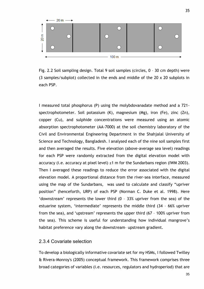
Fig. 2.2 Soil sampling design. Total 9 soil samples (circles, 0 – 30 cm depth) were (3 samples/subplot) collected in the ends and middle of the 20 x 20 subplots in each PSP. ............................................................................................. 35

Fig. 2.3 Effects of covariates inferred from the best GAMs fitted to the abundances of the four prominent mangrove species in the Sundarbans. The solid line in each plot is the estimated spline function (on the scale of the linear predictor) and shaded areas represent the 95% confidence intervals. Estimated degrees of freedom are provided for each smoother following the covariate names. Zero on the y-axis indicates no effect of the covariate on mangrove abundances (given that the other covariates are included in the model). Covariate units: soil salinity = dS m-1, elevation = m (above average-sea), NH4 = gm Kg-1, P = mg Kg-1, K = gm Kg-1), Mg = gm Kg-1, Fe = gm Kg-1, URP = % upriver, DAS = density of all stems for each plot, and historical harvesting (HH) = total number of harvested trees in each plot since 1986. ..................... 43

Fig. 2.4 Spatial density ha-1 of the mangrove species in the Sundarbans based on habitat-based models (GAMs). Areas inside the bold black lines represent the three protected areas. .......................................................................................... 45

Fig. 2.5 Spatial density ha-1 of the mangrove species in the Sundarbans based on geostatistical technique (OK). Areas inside the bold black lines represent the three protected areas. .............................................................................. 46

Fig. 2.6 Spatial distributions of the predicted abundance differences between the GAMs and ordinary kriging for the four species. ................................................ 47

Fig. 3.1 Permanent Sample Plots (PSPs) in the Sundarbans, Bangladesh. Black triangles, green pentagons, and orange circles represent the PSPs located within the hypo-, meso- and hypersaline ecological zones, respectively. ................................. 59

Fig. 3.2 Biodiversity partitioning scheme used in this chapter to explain spatial subcommunity (SC) alpha, beta, and gamma diversity structures across the ecological zones (i.e. hypo-, meso-, and hypersaline zones) and the whole ecosystem (Sundarbans) in four historical time points (in 1986, 1994, 1999 and 2014), and to investigate temporal dynamics in species composition across the individual subcommunities as well as the individual ecological zones over the 28 years. ..... 60

Fig. 3.3 Spatial subcommunity alpha, beta, and gamma diversities (viewpoint parameter, q = 1) in the ecological zones of the Sundarbans in four time points since 1986. .. 66

Fig. 3.4 Spatial distributions of subcommunity alpha, beta and gamma diversities (for viewpoint parameter, q = 1) over the entire Sundarbans generated through ordinary kriging. The black contours represent the three protected areas. ................... 67

Fig. 3.5 Spatial maps showing the distributions of temporal change in subcommunity beta diversity (viewpoint parameter, q = 0, 1, and 2) during 1986 – 2014 generated through ordinary kriging. The black contours represent the three protected areas.......... 69

Fig. 3.6 Mangrove species range change during 1986 – 2014 in the Sundarbans. ......... 72

Fig. 4.1 Sampling sites (triangles) in the Sundarbans, Bangladesh. Blue areas represent water bodies. ................................................................................. 81

Fig. 4.2 Effects of covariates inferred from my best GAMs fitted to the biodiversity indices for q = 1. The solid line in each plot is the estimated spline function (on the scale of the linear predictor) and shaded areas represent the 95% confidence intervals. Estimated degrees of freedom are presented for each smooth following the covariate

8

names. Zero on the y-axis indicates no effect of the covariate on biodiversity index values. Covariate units: CS = total number of individuals in each plot, URP = % upriver, soil salinity = dS m-1, DR = distance (m) of each plot from the riverbank, Historical harvesting (HH) = total number of harvested trees in each plot since 1986, silt (%), disease prevalence (DP) = total number of diseased trees in each plot since 1986, P = mg Kg-1 and K = gm Kg-1. ......................................................... 89

Fig. 4.3 Spatial distributions of SC alpha, beta and gamma diversities (for q = 0 - 2) over the entire Sundarbans generated through GAMs. Higher values of α and γ indicate greater species diversity and community contribution to the overall diversity of the ecosystem. Lower values of ρ indicate greater heterogeneity in species composition (i.e. community distinctness) and higher values of ρ represent greater representativeness (i.e. homogeneity) in species composition. The black contours represent the three protected areas. ..................................................... 91

Fig. 5.1 Productivity and stress levels in plant species are governed by community composition, functional traits and spatio-temporal environmental heterogeneity, but these three determinants also interact with each other in non-trivial ways. ...... 101

Fig. 5.2 Sampling sites (triangles) for species, environmental and trait data collection in the Sundarbans, Bangladesh. Blue areas represent water bodies. ................... 105

Fig. 5.3 Flow chart of the different ecological hypotheses compared via model selection. The different versions (I to IX) of my model were constructed by partitioning the variability in the data in different ways to estimate trait-environment relationships (TER) across multiple species by taking account of the intraspecific trait-trait relationships (TTR) at various hierarchical levels. The performances of the trait-based models were evaluated using DIC (the deviance information criterion, whose numerical value is displayed under each model), with arrows denoting tests made. Black arrows indicate that a new model improved DIC over the older model, red did not, solid arrows point to new models that were selected (the models outlined in black). Dashed arrows point to new models that were not selected (the models outlined in red). ............................................................................. 110

Fig. 5.4 Effects of environmental drivers (URP = upriver position) on the functional traits (Canopy height = Height, SLA = specific leaf area, WD = wood density, LS = leaf succulence) and intraspecific covariation among the functional traits. Each circle represents a species. Species are ordered (left to right, then top to bottom) based on their overall abundance (e.g. E. agallocha1 is the most abundant and S. apetala9 is the least abundant species). The fill-colours of the circles indicate the type and strength of the trait response (red for a negative response and blue for a positive one, see scale on right). A dashed circle around all 9 species indicates that the average species trait response to this environmental driver is strong (negative or positive, i.e. 95% credible intervals do not include 0). Regarding intraspecific covariation among the traits, the colour gradient represents the posterior correlations between traits. Posterior means and 95% credible interval values for the parameters are presented in Tables 5.1 and 5.2. ...................................... 113

Fig. 5.5 Current status (first column) and worst-case scenario for the year 2050 (second column), of community-weighted posterior mean of tree canopy height (Height), specific leaf area (SLA), wood density (WD), leaf succulence (LS) and forest productivity (FP) in the Sundarbans world heritage ecosystem. Uncertainties related to these forecasts are mapped as the posterior probability of deterioration (see section 5.3.4 and Appendices 5B & 5C) in the third column. Deterioration is considered to be a decrease in productivity and growth trait (Height and SLA) values, or an increase in survival trait (WD and LS) values. .................................... 119

Fig. 5.6 Bar charts show the response of the ecosystem to each of five future stress scenarios, E1 to E5, representing a 10% to 50% increase in both salinity and siltation for the whole Sundarbans ecosystem by 2050. (A) shows mean percentage decline in whole ecosystem productivity; (B) shows mean percentage decline in community

9

canopy height (CH) and community specific leaf area (SLA), and increase in community wood density (WD) and community leaf succulence (LS); (C) shows mean percentage decline in CH and SLA, and increase in WD and LS for four prominent mangrove tree species under five future stress scenarios. The species short-hands are Excoecaria agallocha (Ea), Ceriops decandra (Cd), Xylocarpus mekongensis (Xm) and Heritiera fomes (Hf). Decreases in CH and SLA and increases in LS and WD are considered to be deteriorations in the traits. ........................................... 120

Fig. 5.7 Current status (first column) and worst-case scenario for the year 2050 (second column), of posterior mean of tree canopy height for four prominent mangrove tree species in the Sundarbans world heritage ecosystem. Uncertainties related to these forecasts are mapped as the posterior probability of a decrease in canopy height in the third column. ............................................................................ 122

Fig. 5.8 Current status (first column) and worst-case scenario for the year 2050 (second column), of posterior mean of tree SLA for four prominent mangrove tree species in the Sundarbans world heritage ecosystem. Uncertainties related to these forecasts are mapped as the posterior probability of a decrease in SLA in the third column. ................................................................................................. 123

Fig. 5.9 Current status (first column) and worst-case scenario for the year 2050 (second column), of posterior mean of tree wood density for four prominent mangrove tree species in the Sundarbans world heritage ecosystem. Uncertainties related to these forecasts are mapped as the posterior probability of an increase in wood density in the third column. ............................................................................ 124

Fig. 5.10 Current status (first column) and worst-case scenario for the year 2050 (second column), of posterior mean of tree leaf succulence for four prominent mangrove tree species in the Sundarbans world heritage ecosystem. Uncertainties related to these forecasts are mapped as the posterior probability of an increase in leaf succulence in the third column. ......................................................................... 125

10

Acknowledgements

First of all, I wish to thank my mentors — Jason Matthiopoulos and Richard Reeve.

I am incredibly lucky to have dedicated mentors like you. My enthusiasm for work

has just increased day by day during the last four years because of your care,

patience, support and trust on me. Jason, I should reveal that you are the most

influential person in my life. My perspectives on life and science have been refined

in many ways in the last four years. I am privileged to have you as my mentor and

friend. Richard, I have learnt from you how to dig deep into research. Thank you

for your willingness to meet me at short notice every time. I will miss you both.

Special thanks to my external examiner – Bill Kunin from the Faculty of Biological

Sciences, University of Leeds and internal examiner - Grant Hopcraft. I enjoyed

the viva, and your comments on the thesis has been extremely useful. I also thank

my assessors — David Bailey and Barbara Helm. Your external perspective on my

work has been helpful. David, your advice on work-life balance has changed my

lifestyle for sure. You and Jason were always keen to see me going back to family

in Bangladesh every five months. It always gave my family and me a pleasant

feeling. I will always be grateful. I would also like to thank Jill Thompson from the

Centre for Ecology and Hydrology. You were very much passionate about my

project and made valuable contributions to my soil and trait sampling designs. I

would like to say a special thanks to Jana Jeglinski. I could not start producing my

spatial maps without your GIS tips. I would also like to thank Sonia Michell for

helping me understanding the biodiversity quantification codes.

I am grateful to the Commonwealth Scholarship Commission, UK for funding my

PhD studentship. Terry Jacques, Juliette Hargrave and Ellie Fixter – thank you for

your kind helps in managing and extending my scholarship. Jason, you spent your

Glasgow University start-up fund for my field work. Thank you again.

Everybody at the Bangladesh Forest Department was extremely helpful in all

aspects of my fieldwork. Special thanks to Younus Ali, Zaheer Iqbal Ezaz, Jahir

Akon, Nirmal K Paul and Mariam Akhter for sharing the past vegetation data. I

would like to thank Amir Hossain Chowdhury and Zahir Ahmed for giving all logistic

supports during my eight months long fieldwork. I would also like to thank Anwarus

Salehin and Mofazzal Hussain: without your field training, it was not possible for

11

me to find the permanent sample plots in the vast Sundarbans. Thank you, Hasan,

for your six months’ continuous efforts to gather past scattered plot data into

excel files. That was very kind of you. Thank you, Kanak Babu, for offering

accommodation, food and transport when I was helpless for a week. You might

have retired from your Forest Ranger job already. Wish you a happy and healthy

country life.

I am extremely grateful to every one of my fieldwork team: Mahadee Hassan

Rubel, Sourav Das, Niam Jit Das, Harun Rashid Khan, Hasan Murshed, Md.

Qumruzzaman Chowdhury. You all knew that there was always life risk from tigers,

heat strokes, storms and venomous insects in the Sundarbans — but you decided

to help this research my friends. You all suffered a lot. I am not sure I could do

the same for you. I am indebted to all of you forever.

Suvash - you were seriously injured while fixing the engine boat and we

hospitalised you. I still feel guilty for that. You sent us your handmade food couple

of days later. You were so kind to us! I wish you are earning more now-a-days to

afford education for your lovely boy. Tokin — you are a real hero. You owned the

fieldwork. We could reach every plot because of your fearless boat sailing. You

still phone me to know the progress of the research. Thank you mate!

Special thanks to my colleagues: Nusrat Islam and Sontosh Deb from the FES

department in SUST (Bangladesh) for helping me measuring the leaf and wood

samples. You added extra six months to my life. I would also like to thank Md.

Nazrul Islam and Jahurul Alam from SUST. I could start analysing my data

immediately after the fieldwork only because of your restless soil sample analysis,

even during the university vacations.

I would like to thank my friends (Jungle team) in Bangladesh: Nahida Zafrin,

Muhsin Aziz Khan, Amina Pervin, Mohasin, Lisa, Farjana Siddika Rony, Avik Sobhan,

Badrun Nahar, Fahmi and Salahuddin. When I was in Scotland you all visited my

lonely house in Bangladesh routinely to cheer up by wife and kids. We are simply

lucky to have you in our lives.

12

I would like to say a special thanks to John Laurie, Lorna Kennedy, Florence

McGarrity and Lynsay Ross. You all supported me in many ways in the institute.

Elaine Ferguson, Rebby Brown and Francesco Baldini — you all are amazing guys!

I am lucky that it was not all about science that occupied my life in Scotland. Neil

Metcalfe, Jason Matthiopoulos and Julio Benavides — I enjoyed playing and

discussing music with all of you. I will miss the band and your company.

Valia, Jason, Spyros, Merlin – thank you all for keeping my social life alive in

Glasgow. My family is indebted to you all for your love. Valia — you liked my

classical music in Mohan veena although I am a poor performer. I promise to send

you my new compositions when arrive. Spyros — you are so lovely and creative.

Merlin — you are so innocent! Love you all.

Last of all, I would like to thank my wife — Suma and our little boys — Rishav and

Riddhiman. This thesis is nothing but a reflection of your sacrifices. I promise to

stay home more and to go for forest camping soon. Mom - you are certainly happy

to see from the sky that your boy has done this……………

13

Author’s Declaration

I hereby declare that the work presented in this thesis is my own unless otherwise

stated or acknowledged. No part of this thesis has been submitted for any other

degree. The following lists the contributions made to the material in this thesis

by the co-authors and collaborators:

Chapter 2. Published as: “Sarker, S. K., Reeve, R., Thompson, J, Paul, N.K., &

Matthiopoulos, J., 2016. Are we failing to protect threatened mangroves in the

Sundarbans world heritage ecosystem? Scientific Reports, 6, 21234; doi:

10.1038/srep21234.” SKS, JM, RR and JT designed research, fieldwork was carried

out by SKS with assistance from NKP, SKS analysed data with advice from JM and

RR, and SKS prepared the manuscript with comments and edits from JM, RR, JT

and NKP.

Chapter 3. Submitted to ‘Biological Conservation’ as: “Sarker, S. K., Reeve, R.,

Mitchell, S. N., & Matthiopoulos, J., Spatial contraction of distinct and diverse

mangrove communities in the Sundarbans world heritage ecosystem”. SKS, JM

and RR designed research; SKS collected field data; SKS analysed data with

biodiversity quantification code help from SNM and advice from RR and JM; and

SKS prepared the manuscript with comments and edits from JM and RR.

Chapter 4. Submitted to ‘Diversity and Distributions’ as: “Sarker, S. K., Reeve,

R., & Matthiopoulos, J., Modelling mangrove spatial biodiversity in the

Sundarbans World Heritage Ecosystem: A baseline for conservation”. SKS, JM and

RR designed research; SKS collected field data; SKS analysed data with advice

from RR and JM; and SKS prepared the manuscript with comments and edits from

JM and RR.

Chapter 5. Under review in ‘Proceedings of the National Academy of Sciences’ as:

“Sarker, S. K., Reeve, R., & Matthiopoulos, J., Solving the fourth-corner problem:

Forecasts of whole-ecosystem primary production from spatial, multispecies,

trait-based models”. SKS, JM and RR designed research; SKS collected field data;

The original concept of the modelling approach and primary code came from JM;

RR extended the modelling approach and contributed codes; SKS analysed data

14

with advice from RR and JM; SKS prepared the first draft and all authors then

contributed equally to prepare the final draft.

Swapan Kumar Sarker

September 2017

15

Abbreviations

ACEP Atlantic, Caribbean and Eastern Pacific

BFD Bangladesh Forest Department

CS Community size

DAS Density of all stems for each plot

DP Disease prevalence

DR Distance of each plot from the nearest riverbank

FP Forest productivity

HH Historical harvesting

HSM Habitat Suitability Model

IWP Indo-west Pacific

LS Leaf succulence

MC Metacommunity

PAN Protected area network

PSP Permanent sample plots

REDD Reduced Emissions from Deforestation and Degradation

SC Subcommunity

SLA Specific leaf area

16

SLR Sea level rise

TER Trait-environment relationships

TTR Trait-trait relationships

URP Upriver position

WD Wood density

Chapter 1 . General Introduction

1.1 What are mangroves?

Mangroves are woody plants that grow at the interface between land and sea.

They first appeared along the shores of the Tethys Sea and then diverged from

their terrestrial relatives during the Late Cretaceous to Early Tertiary (Ricklefs et

al. 2006). Mangrove forests (30°N and 30°S latitude, 1.37-1.5x105 km2) occur in

the dynamic tropical and subtropical intertidal zones (Giri et al. 2011) and consist

of approximately seventy taxonomically diverse plant species from two plant

divisions, twenty-seven genera, twenty families and nine orders (Duke et al.

1998). Mangroves have many highly specialized adaptations to cope with extreme

environmental conditions such as saline anaerobic sediments, high temperature

and regular flooding (Mitra 2013). The adaptation mechanisms in mangroves are

mainly of three forms: morphological, physiological and anatomical (Naskar &

Palit 2015). Morphological adaptations in many mangroves include

pneumatophores (breathing roots) to grow in anaerobic sediments and viviparous

propagules to promote seed dispersal and formation of new forest stands.

Physiological adaptations include salt exclusion, extrusion or accumulation to

reduce salt stress on plant body. Anatomical adaptations may include thick cuticle

and sunken stomata to ensure efficient water use by mangroves under limited

freshwater availability. Collectively, these mechanisms ensure the long-term

persistence and propagation success of mangroves living under extreme

environments (Duke et al., 1998).

Based on the development of adaptive mechanisms over time and habitat

preferences, mangrove plants are categorized into two groups: exclusive and non-

exclusive mangroves (Wang et al., 2010). Exclusive mangroves are highly adapted

and their geographic ranges are strictly confined to the intertidal environmental

settings (they do not expand into terrestrial communities). On the other hand,

non-exclusive mangroves lack such derived traits and tend to grow in a relatively

benign environment of the intertidal zone. They can even expand their ranges

towards terrestrial plant communities (Tomlinson 1986). For example, the flagship

18

species of the Sundarbans mangrove ecosystem – Heritiera fomes – is a non-

exclusive species while the other major species such as Excoecaria agallocha,

Ceriops decandra and Xylocarpus mekongensis are exclusive mangrove species.

These species show a number of differences in their life-history and morphological

traits and reproductive processes. H. fomes is an evergreen mangrove tree species

that grows up to 25 m in height and produces pneumatophore. It regenerates

through seed and the germination type is hypogeal (Mahmood 2015). The

regeneration is more successful under moderate crown cover than the open areas.

This species has moderate light demands although prefers shade at the early stage

of growth (Siddiqi 2001). Flowering time for this species is April – June and the

fruiting time is May – July. E. agallocha is a deciduous tree that grows up to 5 –

15 m with irregular crown structure. The species mostly shows epigeal germination

and do not have pneumatophores. It also has the ability to copice (Mahmood 2015).

Flowering time for this species is April – July and the fruiting time is May –

September. Ceriops decandra is an evergreen, slow growing tree that grows up to

4 m in height and can survive for long periods under extreme environmental

conditions. The species shows viviparous germination and also has good coppicing

ability (Mahmood 2015). Flowering time for this species is March – May and the

fruiting time is April – July. X. mekongensis is a deciduous tree that grows up to

20 m in height with peg or cone-shaped pneumatophores. Germination type is

hypogeal in this species. Flowering time for this species is March – May and the

fruiting time is April – August (Siddiqi 2001).

1.2 Mangroves are threatened world-wide

Mangrove forests support coastal livelihoods worldwide and provide numerous

ecosystem services, including nutrient cycling (Feller et al. 2010), storm/tsunami

protection (Ostling et al. 2009), carbon sequestration (Alongi 2014), and fisheries

production (Carrasquilla-Henao & Juanes 2017). Mangroves are the most carbon-

dense forests in the world (1,023 Mg C ha-1) (Donato et al. 2011). The estimated

monetary value of the ecosystem services provided by mangrove forests is US

$4185 ha-1 y-1 (Friess 2016). Despite such ecological and economic contributions,

mangroves are declining rapidly because of land clearing, coastal development,

over-harvesting, aquaculture expansion, altered hydrology, nutrient over-

19

enrichment and changes in rainfall and sea surface temperature (Polidoro et al.

2010; Daru et al. 2013; Ghosh et al. 2017). Since the 1950s, the world-wide

mangrove forest coverage has declined by 50% (Feller et al. 2010) and the

geographic range and population sizes of most of the mangrove plant species have

contracted (Polidoro et al. 2010). The current rate of mangrove deforestation is

1-2% per year (Alongi 2015). Different aspects of climate change such as sea level

rise (SLR), altered precipitation patterns and increased temperature and

storminess may further accelerate the loss (Ward et al. 2016). This loss and

degradation may seriously limit the capacity of mangroves to provide valuable

ecosystem services for current and future generations.

1.3 Modelling mangrove abundance

The influence of climate change on mangrove forests’ worldwide distribution is

now well accepted. Studies have shown differential responses of mangroves to

fine-scale variations in salinity (Alongi 2015; Banerjee et al. 2017; Hoppe-Speer et

al. 2011), nutrients (Naidoo 2009; Reef et al. 2010), and hydroperiod (Crase et al.

2013). Hence, future global climate scenarios and changes in fine-scale

environmental conditions may cause species compositional shifts and range

contraction (in an adverse situation, e.g. drought and high salinity) or expansion

(in suitable condition, e.g. adequate rainfall, low salinity and improved nutrient

supply) of individual mangrove species. Quantifying the relationship between

environmental variables and observed species abundance or occurrence using

habitat suitability models (HSMs), has been a widely used approach to address

these challenges for diverse taxa including upland plants (Smolik et al. 2010;

Pottier et al. 2013), birds (Moudrý & Šímová 2013), butterflies (Eskildsen et al.

2013), fish (Gasper et al., 2013), seals (Anderwald et al. 2012), and dolphins

(Hastie et al., 2005). Theoretical background and practical guidelines for

constructing HSMs have been explicitly described by Guisan & Zimmermann

(2000), Austin (2002), Guisan & Thuiller (2005), Franklin (2010) and Miller (2010).

HSMs are static in nature and assume equilibrium or pseudo-equilibrium between

the environment and observed species patterns. These static models fail to

capture the response of species under changing environmental conditions and

have limited ability to cope with non-equilibrium situations (e.g. invasion, climate

change) because they assume that habitats are closed, stable and without

20

competition (Guisan & Zimmermann 2000; Dormann 2007). Despite such

fundamental limitations, HSMs have been widely used for forecasting or

hindcasting species distributions in space and time (Elith & Leathwick 2009). The

outputs of HSMs — species distribution/density maps — can be used for identifying

critical habitats of threatened mangrove species. HSMs can also be used to locate

appropriate mangrove restoration sites by matching maps of critical

environmental variables and species historical ranges or habitat preferences

(Hirzel & Le Lay, 2008). HSMs have been increasingly used to project the potential

effects of global warming on species distributions and ecosystem properties

(Franklin 2010). Global biodiversity databases (e.g. GBIF, BISS etc.) have little

information on mangroves (Ellison 2001). In this context, HSM research on

mangroves can contribute baseline data in these databases. So far, mangrove-

related global and regional conservation work has not focused on species-specific

distributions in space although such information about either abundant or

endangered species is important for identifying critical habitats and no-take zones

and also for establishing coastal protected areas (Polidoro et al. 2010).

Mangrove modelling research has been dominated by topics such as mangrove

demography (Khoon & Eong 1995), stand structure and dynamics (Luo et al., 2010;

Rakotomavo & Fromard, 2010), ecosystem services (Barbier et al. 2011), food

webs (Siple & Donahue 2013), evolution and molecular ecology (Daru et al. 2013;

Triest 2008) and biological invasion (Geller et al., 2010). Moreover, application of

remote-sensing technology to provide spatio-temporal information on mangroves

has been an active area of research during the last two decades (Giri et al., 2011;

Heumann, 2011; Kuenzer et al., 2011). However, the use of HSMs for mangroves

has been limited. Only recently, Record et al. (2013) provided the first example

of applying species and community distribution models to coastal mangroves

worldwide. However, fine-scale environmental data-driven regional or local HSMs

that offer realistic predictions for both species and habitat conservation (Franklin

2010) are limited for mangroves.

21

1.4 Modelling mangrove biodiversity

1.4.1 Biodiversity quantification: state-of-the-art

Understanding the processes that shape biodiversity and explaining biodiversity

patterns across space and time are crucial for identifying vulnerable ecosystems,

habitats or species and for developing realistic conservation plans (Meynard et al.

2011). These processes are, however, scale-dependent. For example, biodiversity

at a local scale may be related to competition or random dispersal whereas

regional diversity may be related to environmental filtering (Swenson et al. 2012).

Two prominent theories — ‘niche theory’ (Hutchinson 1957) and ‘neutral theory’

(Hubbell 2001) — have quite different explanations about the processes that shape

biodiversity. Niche theory asserts that the amount of resource use varies across

species, so only species having differentiated niches can coexist in a particular

ecological community. The neutral theory assumes that community individuals

have the same chance to reproduce and death, and relative abundances of species

vary for demographic stochasticity or ‘ecological drift’. It further assumes that

demographic processes take place at the local scale and demographic drift may

be responsible for species extinction. Demographic drift may also be responsible

for species extinction from the regional species pool. The regional species pool

may gain novel species via speciation and contributes to local diversity via

propagule dispersion. The neutral theory of Hubbell thus proposes ‘limited

dispersal’ instead of ‘niche specialization’, as the main mechanism responsible for

spatial variation across ecological communities.

Biodiversity is simplified by partitioning regional species diversity (γ) into local (α)

and turnover (β). α (alpha) diversity represents species diversity of a specific site,

β (beta) diversity represents species compositional variation among sites, and γ

(gamma) diversity is the sum of diversity for the various sites within an ecosystem.

Species richness and numerous indices that incorporate relative abundances of

species are two principle measurement schemes of alpha diversity. α diversity can

be estimated in many ways (Maurer & Mcgill 2011). However, Shannon’s index of

diversity (Shannon & Weaver 1949) and measures based on Simpson’s

concentration (Simpson 1948) are the most commonly used indices. Jost (2006,

2007) has strongly criticized the use of index values of these indices in making

22

ecological statements and suggested using the ‘effective number of species’ which

he termed ‘true diversity’.

β diversity can be defined in two ways: directional turnover and non-directional

variation. In the case of directional turnover, species compositional change is

measured along a specified gradient (e.g. spatial, temporal or environmental),

and in case of non-directional variation, variation in species composition is

measured without reference to any specific gradient (Legendre & De Cáceres

2013). Both β diversity versions are frequently used to explain the connections

between local and regional diversity, and for visualizing spatial patterns of species

assemblages (De Cáceres et al. 2012). Various β diversity indices have been

proposed to quantify species compositional variation (directional or non-

directional). Whittaker (1960) first proposed a non-directional β diversity index

for species richness (β = γ/α), and Nekola & White (1999) developed a directional

β index by introducing the slope of the similarity decay in species composition

with geographic distance. After these initial approaches, the number of indices

has been increasing. Currently, the most popular indices belong to two families:

additive (α + β = γ)(Lande 1996) and multiplicative (α x β = γ)(Whittaker 1972).

While debates on several aspects of diversity measurements (e.g. partitioning

diversity, scale, theoretical clarity, biological meaning) are ongoing (Barwell et

al. 2015), a variety of approaches have been taken by ecologists (Jost, 2006, 2007,

2010; Mendes et al., 2008; Tuomisto, 2010a, 2010b; Veech & Crist, 2010) to

develop a unified index of diversity measurement. Most of these approaches,

abundance-based in nature, have tried to integrate several components of

diversity (e.g. evenness, scale etc.) into a single unified equation. However,

Leinster & Cobbold (2012) criticized these approaches for not accounting for the

species relative abundances. Reeve et al. (2016) have recently proposed a unified

framework that resolves these problems and offers direct diversity comparison

between constituent communities of an ecosystem, thus allowing identification of

distinct, diverse or homogeneous communities. The main motivation behind their

approach is to overcome the limitations of traditional diversity indices and to

make diversity comparisons easier and informative.

23

1.4.2 Mangrove biodiversity research: state-of-the-art

Spatial modelling of distributions of individual species has been, so far, the most

popular strategy in ecology and biogeography (Franklin 2010). Community-level

biodiversity modelling is gaining popularity for its ability to account for the rare

species and to combine complex species and environmental data into a structured

form which allows us to produce various spatial outputs such as maps of diversity

indices, community types (sites with similar species composition), species groups

(species with similar distributions), and gradients of compositional variation

(Bonthoux et al., 2013). A variety of approaches: (1) ‘assemble first, predict

later’, (2) ‘predict first, assemble later’ and (3) ‘assemble and predict together’

(Ferrier & Guisan 2006) are followed to produce these outputs. In the ‘assemble

first, predict later’ approach, biological survey data are first used to estimate

plot-level biodiversity indices which are then modelled as a function of

environmental covariates. In the ‘predict first, assemble later’ approach,

individual species in a study area are first modelled separately as a function of

the environmental covariates to generate species distribution layers and then

these layers are combined to calculate biodiversity indices for all grid cells. In the

‘assemble and predict together’ approach, a single integrated modelling

framework is first used to predict the spatial distributions of all species

simultaneously and then these predictions are used to calculate biodiversity

indices for all grid cells. While these approaches have been widely applied to

identify hotspots and to prioritize conservation sites for a variety of taxa (e.g.

upland tree species, birds, and fish), they have rarely been used for the mangrove

taxa.

Testing ‘zonation’ (distinct ordering of mangrove plants from shore to inland) and

explaining the ‘biodiversity anomaly’ (mangrove species richness declines when

we move along the latitudinal gradient) are the two research agendas that have

dominated the mangrove biodiversity literature. Numerous studies have tested

the existence of mangrove species zonation patterns. Although zonation is

considered a common pattern in mangrove distributions world-wide (Siddiqi 2001),

Bunt (1996) and Bunt & Stieglitz (1999) could not identify any clear-cut mangrove

distribution patterns in Australia. Ellison et al. (2000) criticized the previous

studies for being descriptive and tested species zonation patterns in the

Bangladesh Sundarbans using quantitative methods. They did not notice any

24

distinct species zonation patterns. The number of mangrove plant species declines

when we move along the latitudinal gradient – highest species richness (58 plant

species) in the Indo-west Pacific (IWP) zone and lowest (12 plant species) in the

Atlantic, Caribbean and Eastern Pacific (ACEP) regions. Mangrove ecologists put

tremendous efforts to explain the cause of this ‘anomalous’ drop in species

richness from IWP to ACEP (Ellison et al. 1999; Ellison 2001; Ricklefs et al. 2006).

Limited understanding of how fine-scale environmental variations and human

pressures effect mangrove communities, has obstructed the success of mangrove

conservation initiatives in many countries (Lewis 2005). Mangrove biodiversity

research programs have mostly relied on the species richness index which does

not account for between-species population variability. Robust abundance-based

unified equations for biodiversity quantification could be a promising tool to

capture local spatial variability in species diversity and composition in the tropical

mangrove ecosystems.

1.5 Quantifying trait-environment relationships

A central challenge in plant ecology is to understand and predict the spatial and

temporal changes in species composition and the associated changes in ecosystem

function under varying biotic and abiotic conditions. While using species-centric

approaches has been a common practice to handle this challenge, plant ecologists

now consider trait-based approaches as the most appropriate choice (Diaz et al.

2007; Laughlin 2014; Chain-Guadarrama et al. 2017). Trait-based approaches are

based on the idea that the fitness of plant species depends on how their traits

respond to environmental drivers, thus facilitating more mechanistic prediction of

species-, community- and ecosystem-level attributes (e.g. abundance, community

composition, and biomass productivity etc.) under changing environmental

conditions (Cadotte et al. 2011; Reich 2014). Plant functional traits are any

measurable feature (morphological, physiological or anatomical) that influence a

plant’s performance (Violle et al. 2007). Thus, functional traits play important

roles in determining: which plant species can grow and survive under what

environmental conditions, to what extent they acquire resources and maintain

primary growth, and how they interact with co-existing species (Westoby & Wright

2006). How these roles are mediated by dynamic environmental conditions in

25

natural forest ecosystems, collectively, influence the ecosystem processes,

functioning and services (Hooper et al. 2005; Cadotte et al. 2011).

Disentangling the association between traits and environmental drivers i.e.

“performance filter” (Webb et al. 2010) is the building block of trait-based

ecology because predicting filtered trait distributions based on a projection of the

performance filter across space and time can determine species abundance and

community composition which in turn defines ecosystem functions and services

under changing environment. However, linking traits to environmental variables

and abundances has been a long-standing problem known as the fourth-corner

problem in community ecology. Ecologists have proposed both multivariate

(Dolédec et al. 1996; Legendre et al. 1997; Dray & Legendre 2008; ter Braak et al.

2012; Dray et al. 2014) and univariate (Pollock et al. 2012; Jamil et al. 2012; Jamil

et al. 2013; Jamil et al. 2014; Brown et al. 2014) approaches to resolve the

problem. Existing multivariate approaches (e.g. RLQ ordination, permutation tests

etc.) offer a broad qualitative impression of trait-environment associations and

help in selecting important traits and environmental variables in a trait-based

study. However, these approaches have limited ability to quantify the strength of

the associations between traits and environmental drivers. On the other hand,

recent advancements in trait-based univariate (regression) approaches offer the

flexibility of model selection, validation, and predictions. Although these

approaches may potentially scale up individual traits to the community and

ecosystem level processes (Funk et al. 2017), currently their usage is limited for

single species and single traits.

Persistent environmental pressures may eliminate species over ecological time

scales (species sorting) and modify trait values over evolutionary time scales

(natural selection), resulting in altered species composition, relative abundance,

and finally productivity in local communities (Verberk et al. 2013). Species sorting

and natural selection do not act independently on a single trait, but rather, on

species whose survival in a specific environment is controlled by multiple

interacting traits. However, existing trait-based univariate approaches mostly

deal with single species (Jamil et al. 2012) and have limited statistical ability to

model multiple species, traits, and environmental variables simultaneously and to

incorporate complex interactions between multiple traits of multiple competing

26

species under a dynamic environment. These shortcomings thus may yield

excessively uncertain predictions when forecasting species, community and

ecosystem responses under future environmental scenarios (Webb et al. 2010;

Verberk et al. 2013; Violle et al. 2014).

Therefore, substantial methodological improvements are still required for linking

the underlying concepts of trait-environmental relationships to quantitative

approaches that will allow a predictive basis to community ecology and provide

theoretical linkages between community ecology, ecosystem ecology, and

functional biogeography. Webb et al. (2010) stated that traits-based ecology is

now at a critical juncture where further advancements require an integrated

quantitative approach that can analyse hierarchically structured trait data

consistently to explain the dynamic nature of the trait–environment relationship

and allow for robust spatial and temporal predictions of trait distributions with

precise estimates of uncertainties. Verberk et al. (2013) consider that failure in

detecting the response traits, in addressing the linkages and interactions among

traits, and in differentiating which trait combinations maintain plants’ growth and

survival under stress, are the predominant constraints responsible for low

discriminatory power and poor mechanistic understanding of current trait-based

approaches. Funk et al. (2017) have identified three outstanding issues (i.e.

selecting appropriate traits; unfolding intraspecific trait variation and integrating

this variation into models; and scaling functional trait data to community- and

ecosystem-level processes) that need to be resolved to advance traits-based

ecology. To do so they and many others (Webb et al. 2010; Verberk et al. 2013)

have suggested a need for new model development.

1.6 Study site: the Sundarbans

The Sundarbans is Earth’s largest continuous mangrove forest covering 10,017 km2

in Bangladesh and India. This forest is part of the Ganges-Brahmaputra delta which

originated following the fragmentation of Gondwanaland in the early Cretaceous

(Islam & Wahab 2005). The Bangladesh part of the Sundarbans (21°30′ — 22°30′N,

89° 00′ – 89°55′E) covers 6017 km2. Of this 69% is forest land, and the rest

encompasses rivers, small streams and canals. The forest is washed out by the

tide twice a day and its hydrology depends on the fresh water discharge from the

Ganges and the saltwater influx from the Bay of Bengal.

27

The Bangladesh Sundarbans supports the livelihood of 3.5 million coastal people

(Islam et al. 2014), harbours breeding and nursing grounds for many marine

organisms (Sandilyan & Kathiresan 2012), protects them from natural disasters

(Danielsen et al. 2005), and houses the remaining habitats of many globally

endangered plant and animal species (Siddiqi 2001). Because of these

contributions, UNESCO declared the Bangladesh Sundarbans a World Heritage Site

in 1997 (Gopal & Chauhan 2006). It was also declared a globally important RAMSAR

wetland ecosystem under the Ramsar Convention in 1992 (Siddiqi 2001).

The Sundarbans has lost half of its original size within the last 150 years due to

the conversion of mangrove habitats to agricultural land and human settlements

(Siddiqi 2001). Historical forest exploitation, gradual reduction in freshwater flows

(3700 m3/s to 364 m3/s) since the construction of the Farakka dam in India in 1974,

salinity intrusion, oil spills, cyclones, water and soil pollution have severely

degraded the Sundarbans ecosystem by depleting the populations of many

threatened mangroves, including the globally endangered Heritiera fomes (Ellison

et al. 2000). Some studies (Ellison et al. 2000; Iftekhar & Islam 2004; Iftekhar &

Saenger 2008; Mukhopadhyay et al. 2015; Aziz & Paul 2015) have described the

negative effects of these forces on Sundarbans’ forest structure and functions.

Along with the historical and ongoing degradations, different aspects of climate

change, particularly, sea level rise (SLR) (Karim & Mimura 2008) are likely to have

a significant influence on the Sundarbans. However, spatially explicit baseline

information on the remaining populations and spatial distributions, diversity,

species composition, and functions of the mangroves are still lacking. This scarcity

of information has been a major impediment to national and international

conservation efforts in the Sundarbans (Islam et al. 2014; Aziz & Paul 2015).

1.7 Aims of the thesis

The overall aim of this thesis is to quantify the habitat preferences of threatened

mangroves in the Sundarbans world heritage ecosystem, to explore spatial and

temporal dynamics and the key drivers of mangrove biodiversity, and to develop

an integrated approach for predicting functional trait responses of plants under

current and future environmental scenarios. The thesis comprises four data

chapters (Chapters 2 – 5).

28

Chapter 2 determines habitat preferences and develops spatial density maps of

the four most dominant mangrove tree species (i.e. Heritiera fomes, Excoecaria

agallocha, Ceriops decandra and Xylocarpus mekongensis).

Chapter 3 determines the spatial heterogeneity in alpha, beta, and gamma

diversity at four historical time points (1986, 1994, 1999 and 2014) to uncover the

temporal dynamics in species composition in the established ecological zones

(hypo-, meso-, and hypersaline) in the Sundarbans. Specific questions that I ask

here include: Which ecological (i.e. salinity) zone supports the most/least diverse

mangrove communities? Is the most diverse ecological zone also the most

heterogeneous (i.e. variable between plots) in species composition? How has

compositional heterogeneity in the broader ecological zones developed over the

28 years? How has the geographic range and density of mangroves changed since

1986? I also develop spatial biodiversity maps to answer the following questions:

Where are the historical and contemporary biodiversity hotspots located? Which

habitats have changed most in species composition over time?

Chapter 4 uncovers the influences of fine-scale habitat conditions and historical

events in shaping the spatial distributions of mangrove alpha, beta and gamma

diversity. My more specific questions include: What are the key drivers of

mangrove biodiversity? How do the predictive abilities of environmental data-

driven biodiversity models compare with those of covariate-free direct

interpolation approaches? Where are the biodiversity hotspots in the Sundarbans

currently located? Are these hotspots well protected?

Chapter 5 proposes a Bayesian hierarchical modelling approach to quantify trait-

environment relationships for multiple traits, species, and environmental drivers

simultaneously, while accounting for trade-offs between different traits. I then

apply this integrated approach on field data comprising nine prominent tree

species, eight important environmental drivers, and four key plant morphological

traits (canopy height, specific leaf area, wood density, and leaf succulence) and

ask: (1) Which set of theoretical hypotheses, is best supported by the data? (2)

How do the different traits of each species respond to the array of environmental

drivers? (3) Is there covariation between the responses of functional traits? Using

the model-based predictions, I then develop trait and productivity maps under

present and future environmental scenarios.

29

Finally, Chapter 6 provides a broader discussion of previous chapters’ results and

proposals for future improvements.

30

30

Chapter 2 . The spatial distribution and habitat preferences of threatened mangroves in the Sundarbans: Implications for conservation

*Note: This chapter has been published in ‘Scientific Reports’ (Appendix 1)

2.1 Abstract

The Sundarbans world heritage ecosystem is under threat from historical and

future human exploitation and sea level rise. Limited scientific knowledge on the

spatial distributions of the threatened tree species and their habitat requirements

has obstructed conservation efforts in this global priority ecosystem. Using tree

counts and environmental data collected from 110 permanent sample plots (PSPs),

in this chapter, I developed habitat suitability models (HSMs) and species density

maps for the four most dominant mangrove species: Heritiera fomes, Excoecaria

agallocha, Ceriops decandra and Xylocarpus mekongensis. Generalized additive

models of mangrove abundance data revealed steep responses to salinity

gradients. Globally endangered H. fomes abundance declined as soil salinity

increased. Responses to nutrients, elevation and stem density varied between

species. X. mekongensis preferred upstream habitats while the rest preferred

downstream and intermediate-stream areas. Historical harvesting had negative

influences on all species, except E. agallocha. The most suitable habitats of the

threatened species currently occur outside the existing protected area network

(PAN). This study, therefore, recommends a reconfiguration of the existing PAN

to include these suitable habitats and ensure their immediate protection. Finally,

I discuss how the habitat insights and spatial predictions generated by my models

can guide future forest studies and spatial conservation planning.

2.2 Introduction

The mangrove biome (137,760 km2 in 118 countries) is under severe threat. We

have lost nearly 50% of the biome since the 1950s due to deforestation, habitat

degradation and coastal development (Feller et al. 2010). If the current trend of

human exploitation and habitat degradation continues, the whole mangrove biome

may vanish in the next 100 years (Duke et al. 2007). About 16% of the total

mangrove plant species (~ 70) are at elevated risk of extinction and 10% are near-

31

31

threatened (Polidoro et al. 2010). However, we have limited knowledge about the

habitat preferences and current spatial distributions of these threatened plants in

many stressed coastal regions in the tropics, particularly, the Sundarbans, which

is a UNESCO World Heritage Site and a RAMSAR wetland ecosystem of global

importance (Siddiqi 2001).

The Sundarbans contains one third of the global mangrove plant species (Ghosh et

al. 2016) and acts as a repository of numerous globally endangered flora and fauna

(Iftekhar & Islam 2004). However, natural (e.g. tropical cyclones, tsunamis) and

anthropogenic (e.g. tree harvesting, aquaculture, oil spills) pressures (Ellison et

al. 2000; Aziz & Paul 2015) have heavily degraded the Sundarbans ecosystem,

resulting in local extinction of at least three mangrove plant species of the

Bruguiera genus and six mammal species including Javanese rhinoceros

(Rhinoceros sondiacus) and wild buffalo (Bulbulus bulbalis) in the last two

centuries (Iftekhar & Islam 2004). The population of Heritiera fomes, a globally

endangered tree species, has declined by 76% since the 1950s. Nearly 70% of the

H. fomes trees are currently affected by the ‘top dying’ disease (Chowdhury et

al. 2008). Declines in other major mangrove tree species (e.g. Excoecaria

agallocha and Xylocarpus mekongensis) have also been reported (Iftekhar &

Saenger 2008). We also know little about the current spatial distributions of

Ceriops decandra, a globally near-threatened species (Siddiqi 2001).

In the Sundarbans, the freshwater river flows help to modulate salt-water toxicity

and keep the ecosystem suitable for mangrove trees. However, since the

construction of the Farakka dam (in 1974) in the Ganges upstream, the freshwater

supply into the Sundarbans has reduced by 65% (Iftekhar & Islam 2004), resulting

in increased salinity levels, reduced nutrient status, and overall degradation of

the entire ecosystem (Mukhopadhyay et al. 2015). The rate of sea level rise (SLR)

along the Bangladesh coast was substantially higher than the global average in the

last century (Karim & Mimura 2008). Future SLR is likely to alter the habitat

conditions, regional hydrology, vegetation structure and functions in the

Sundarbans (Ghosh et al. 2016). Therefore, ongoing habitat degradation and

future SLR together may alter the current spatial distributions of these mangrove

species and forest community composition.

32

32

Determining the drivers and spatial distributions of threatened species is vital for

their management and conservation. However, lack of such knowledge has

obstructed the success of conservation initiatives in many countries (Lewis 2005),

including Bangladesh (Islam et al. 2014). Only recently have coastal mangrove

distributions been modelled at global (Record et al. 2013) and regional (Crase et

al. 2015) scales and we are now in urgent need of Habitat Suitability Models

(HSMs), based on fine-scale species abundance and environmental data to assist

us in protecting threatened ecosystems such as the Sundarbans. HSMs and their

outputs (i.e. habitat maps) are widely used during different phases of resource

management and spatial conservation planning (Guisan & Thuiller 2005). These

maps are also used to identify areas appropriate for establishing protected areas,

evaluate threats to those areas, and design reserves (Guisan et al. 2013). For

example, a baseline distribution map of the mangrove species could be an

important tool for the forest managers to make decisions on future mangrove

planting and forest protection via tracking population changes over time.

In this chapter, I used tree counts and environmental data collected from a

network of 110 permanent sample plots (PSPs) in the Sundarbans to generate

spatially explicit baseline information on the distribution and habitat preferences

of the four most abundant mangrove species: H. fomes, E. agallocha, C. decandra

and X. mekongensis. I identified the key environmental variables related to their

spatial distribution and generated species-specific spatial density maps using both

geostatistical and regression approaches. I then demonstrated the potential

applications of these habitat insights and spatial maps for future forest studies,

spatial conservation planning, biodiversity protection and monitoring programs.

2.3 Methods

2.3.1 Study system

The Bangladesh Sundarbans (21°30′ — 22°30′N, 89° 00′ – 89°55′E) is part of the

Earth’s largest river delta at the Ganges-Brahmaputra estuary (Fig. 2.1).

Geologically, the Sundarbans is of recent origin (about 7000 years old) and was

formed through the silt deposition by the Ganges-Brahmaputra river system

(Iftekhar & Islam 2004). The soil is finely textured, poorly drained and rich in alkali

metal contents (Siddiqi 2001). Of its total area (6017km2), about 69% is land and

33

33

the rest comprises rivers, small streams and canals (Wahid et al. 2007). Most parts

of the forest are inundated twice a day. The water level is associated with the

joint effects of the seawater tides and freshwater input from the Ganges.

Freshwater flow increases during the monsoon (June–September) and sharply

drops during the dry season (October to May) due to reduced water influx from

the Ganges. The climate is humid and tropical. Average annual precipitation is

1700 mm. Average maximum annual temperature is between 29.4° and 31.3°C

(Gopal & Chauhan 2006).

2.3.2 Tree surveys

To monitor biodiversity and forest stock the Bangladesh Forest Department (BFD)

established a network of 120 PSPs in the Sundarbans in 1986 (Fig. 2.1). Each PSP

is 0.2 ha in size (100 x 20 m) and divided into 5 20 x 20 m subplots. Of these, 110

PSPs were positioned to represent the ecological zones (i.e. hyposaline,

mesosaline and hypersaline) and the forest types (Iftekhar & Saenger 2008). The

remaining 10 relatively smaller sized PSPs (20 x 10 m) were established to monitor

forest regeneration, and were not considered in this thesis. As part of the 2008 –

2014 forest inventories, my fieldwork team, together with the BFD tagged every

tree with stem diameter ≥ 4.6 cm (because mangroves grow very slowly and this

threshold value has been used in all previous forest inventories in the Sundarbans

since the early 1900’s (Iftekhar & Saenger 2008)), recorded at 1.3 m from the

ground with a unique tree number and recorded tree counts for each of the 110

PSPs.

34

34

Fig. 2.1 Sampling sites (triangles) in the Sundarbans, Bangladesh. The thin grey

lines represent the canals.

2.3.3 Environmental data

Environmental data were collected from all 110 PSPs during January — June 2014.

I adopted a soil sampling design (Fig. 2.2), collected 9 soil samples from each PSP

(to a depth of 15 cm) to account for the within-plot variation in soil parameters.

For soil texture analysis (percentage of sand, slit and clay), I used the hydrometer

method (Gee & Bauder 1986). I determined soil salinity (as electrical conductivity

— EC) in a 1:5 distilled water:soil dilution (Hardie & Doyle 2012) using a soil

conductivity meter — Extech 341350A-P Oyster. I took field measurements for soil

pH and oxidation reduction potential (ORP) using digital soil pH and ORP (Extech

RE300 ExStik) meters. Soil NH4 concentration was measured following the Kjeldahl

method (Bremner & Breitenbeck 1983).

35

35

Fig. 2.2 Soil sampling design. Total 9 soil samples (circles, 0 – 30 cm depth) were

(3 samples/subplot) collected in the ends and middle of the 20 x 20 subplots in

each PSP.

I measured total phosphorus (P) using the molybdovanadate method and a 721-

spectrophotometer. Soil potassium (K), magnesium (Mg), iron (Fe), zinc (Zn),

copper (Cu), and sulphide concentrations were measured using an atomic

absorption spectrophotometer (AA-7000) at the soil chemistry laboratory of the

Civil and Environmental Engineering Department in the Shahjalal University of

Science and Technology, Bangladesh. I analysed each of the nine soil samples first

and then averaged the results. Five elevation (above-average sea level) readings

for each PSP were randomly extracted from the digital elevation model with

accuracy (i.e. accuracy at pixel level) ±1 m for the Sundarbans region (IWM 2003).

Then I averaged these readings to reduce the error associated with the digital

elevation model. A proportional distance from the river-sea interface, measured

using the map of the Sundarbans, was used to calculate and classify “upriver

position” (henceforth, URP) of each PSP (Norman C. Duke et al. 1998). Here

‘downstream’ represents the lower third (0 – 33% upriver from the sea) of the

estuarine system, ‘intermediate’ represents the middle third (34 – 66% upriver

from the sea), and ‘upstream’ represents the upper third (67 – 100% upriver from

the sea). This scheme is useful for understanding how individual mangrove’s

habitat preference vary along the downstream– upstream gradient.

2.3.4 Covariate selection

To develop a biologically informative covariate set for my HSMs, I followed Twilley

& Rivera-Monroy's (2005) conceptual framework. This framework comprises three

broad categories of variables (i.e. resources, regulators and hydroperiod) that are

36

36

believed to control mangrove forest structure and function (Krauss et al. 2008;

Reef et al. 2010; Crase et al. 2013). Resources (i.e. nutrients) are used by plants

and their availability is related to tree productivity. Here, I selected soil NH4, P,

K, Mg, Fe and Zn based upon the detailed explanation of nutrient requirements of

mangrove plants available in the mangrove literature (Reef et al. 2010).

Regulators are non-resource variables that influence the growth and

establishment of mangroves. I employed soil salinity as the main regulator.

Hydroperiod (the duration, frequency and depth of inundation) is recognized as

an important determinant of mangrove distribution (Crase et al. 2013). PSP level

hydroperiod data are not available for the Sundarbans, so I selected elevation as

a proxy that reflects the possible variation in hydroperiod across the Sundarbans.

I also selected URP of each PSP as a covariate to account for the effects of the

river systems on mangrove distributions along the downstream-upstream gradient.

The relative abundance of a mangrove species may influence the abundance of

another through biotic interactions i.e. competition or facilitation (Wisz et al.

2013). In fact, each tree interacts with the trees that are in its neighbourhood

through multiple concurrent interactions (Le Roux et al. 2013). Given the super-

dominance of E. agallocha and H. fomes (see section 2.3.2) and tree structural

complexities (i.e. multiple stems in C. decandra) which might have increased tree

measurement (i.e. diameter) errors, I initially considered two alternative

measures of abundance: (1) density of all stems for each plot, and (2) total basal

area for each plot as biotic variables. HSMs of species with basal area as a

covariate had lower explanatory and predictive powers, compared to models with

density of all stems. Therefore, I selected density of all stems for each plot

(hereafter, DAS) as a simple proxy for biotic interaction.

The Sundarbans has a long exploitation history (Siddiqi 2001). Illegal tree

harvesting is also common (Iftekhar & Islam 2004). Hence, I incorporated historical

harvesting (henceforth, HH) as a covariate in my HSMs due to its potential

influence on present tree densities in the PSPs. HH denotes the number of cut

trees (detected by counting stumps) in each PSP from the first census (1986) to

the last census (2014).

I checked for multi-collinearity in my set of candidate covariates using the vifstep

function of ‘usdm’ package (Naimi 2015) in R 3.2.2 (R Core Team 2016), which

37

37

first calculates Variance Inflation Factors (VIF) for all predictor variables, then

removes the one with highest VIF that exceeds the threshold of 2.5 and repeats

the procedure until no variable with VIF > 2.5 remains. This led to the exclusion

of Zn from my covariate set (Appendix 2A).

2.3.5 Habitat suitability analyses

I used generalized additive models (GAMs) (Wood 2006) with a Poisson likelihood

and a log-link for their ability to handle complex, non-monotonic relationships

between the response and the predictor variables (Guisan et al. 2002). Moreover,

by using non-parametric smoothing functions, GAMs can often construct

biologically insightful relationships between response and covariates without a-

priori hypotheses (Guisan & Thuiller 2005). Smoothed responses used cubic basis

splines executed within the ‘mgcv’ package (Wood 2011) in R.

Using the ‘dredge’ function in the ‘MuMIn’ package (Barton 2015), I fitted

candidate models with all possible combinations of covariates and ranked them

using the Akaike Information Criterion (AIC) (Burnham & Anderson 2002). I then

obtained the relative support for each model by calculating the ∆AIC (the

difference between the best model’s AIC value and the AIC value for each of the

other models). Kullback–Leibler information loss is minimal between models with

∆AIC ≤ 2 (Burnham & Anderson 2002). So, I used the ‘∆AIC ≤ 2’ criterion to select

my confidence set of models for each mangrove species. I then calculated Akaike

weights (AICw) to inspect relative support for each model in the confidence set.

AICw values range from 0 to 1 and the sum of all AICw across the confidence set

is 1. When there was only one model with ∆AIC ≤ 2, it was unambiguous that it

outperformed all possible candidate models. When there were multiple competing

models, I used AIC-weighted model averaging to reduce model selection

uncertainty and bias. I determined Relative Importance (RI) of each covariate by

summing the AICw of the models in which the covariate was retained. RI values

range between 0 and 1, where 0 indicates that the target covariate is never

included in the competing models, 1 indicates inclusion of the covariate in all the

competing models. I ranked the covariates based on their RI values. Residual

diagnostic plots for the best GAMs did not show violations of the Poisson dispersion

assumption.

38

38

Goodness-of-fit of the models was measured using the R2 (coefficient of

determination) statistic between the observed and estimated abundance values.

For validation purposes, I partitioned my dataset into a calibration (88 PSPs, 80%

of the full data) and validation (22 PSPs, 20% of the full data) subsets. The

validation dataset was randomly chosen to cover the whole Sundarbans and was

employed to assess the predictive power of the fitted models via the R2 statistic

applied to the model’s predictions for the validation data. I also mapped the

actual and predicted abundances of both calibration and validation set to check

for any spatial patterns of prediction errors.

2.3.6 Spatial mapping

I mapped mangrove species densities over the entire Sundarbans using two

different approaches: (1) direct interpolation of plot-level raw abundance using

geostatistical methods, and (2) habitat-based predictions from my HSMs.

Environmental data collection is demanding, whereas tree abundance

measurements are taken regularly at the PSPs. Therefore, it is useful to know how

close the predictions of the habitat models were compared to simple interpolation

methods. To directly interpolate individual mangrove species abundances, I used

ordinary kriging (OK), a widely-used interpolation technique. Selecting an

appropriate variogram model is a prerequisite for kriging success. I fitted three

different variogram models to each mangrove: Spherical, Exponential and

Gaussian, and selected the model with least sum of squared errors. The spherical

model offered best fit for H. fomes, the exponential model provided best fit for

E. agallocha and C. decandra, and the Gaussian model for X. mekongensis (see

Appendix 2B for the semivariograms of the species).

For producing covariate surfaces, I fitted Spherical, Exponential and Gaussian

variogram models to each covariate, and selected the model with least sum of

squared errors (see Appendix 2C for the semivariograms of the covariates). I then

used these covariate surfaces (Appendix 2D) to generate model-averaged

predictions of species density over the entire Sundarbans.

Each grid-cell of the interpolated surface was 625 m2 (25m x 25m). The covariate

surfaces were constructed by OK using the ‘gstat’ package (Pebesma 2004) in R.

A protected area network (PAN) comprising three Wildlife Sanctuaries (WS) – East

WS, West WS, and South WS has been operational since the 1970s. I superimposed

39

39

the PAN on my species density maps for evaluating its spatial extent to cover the

current density hotspots of the threatened tree species. I also compared the

predictive abilities of the direct and habitat-based approaches. Here, I used the

normalized root mean square error (NRMSE) statistic derived from the leave-one-

out cross-validation procedure. For normalization, the root mean square error

statistic was divided by the range of the actual species abundances. Both habitat-

based and direct predictions of the mangrove tree abundances were mapped using

the ‘raster’ package (Hijmans 2015) in R. I further mapped the prediction

discrepancy between these two approaches, to look for any spatial patterning in

the prediction errors.

2.4 Results

2.4.1 Tree surveys

A single survey of each of the 110 PSP’s carried out between 2008 — 2014 gave a

total of 49409 trees of 20 species from 13 families and 18 genera (Table 2.1). The

most abundant mangrove tree species was E. agallocha (59.69% of total trees),

followed by H. fomes (30.89%), C. decandra (6.12%) and X. mekongensis (0.82%).

The remaining 16 species were extremely rare comprising only 2.49% of the total

count.

40

40

Table 2.1 Taxonomy and global conservation status of the mangrove species

surveyed in the 110 permanent sample plots (PSPs) in the Bangladesh Sundarbans.

*IUCN global population trend, † Not assessed for the IUCN Red List, LC = Least

concern, DD = Data deficient, NT = Near threatened, VU= Vulnerable, EN =

Endangered, D = Decreasing.

Latin name Family IUCN conservation

status

Global population

trend*

Aegiceras corniculatum Myrsinaceae LC D

Amoora cucullata Meliaceae NA† NA

Avicennia officinalis Avicenniaceae LC D

Bruguiera sexangula Rhizophoraceae LC D

Cerbera manghas Apocynaceae NA NA

Ceriops decandra Rhizophoraceae NT D

Cynometra ramiflora Fabaceae NA NA

Excoecaria agallocha Euphorbiaceae LC D

Excoecaria indica Euphorbiaceae DD D

Heritiera fomes Malvaceae EN D

Intsia bijuga Leguminosae VU D

Lumnitzera racemosa Combretaceae LC D

Hypobathrum racemosum Rubiaceae NA NA

Pongamia pinnata Leguminosae LC Stable

Rhizophora mucronata Rhizophoraceae LC D

Sonneratia apetala Lythraceae LC D

Talipariti tiliaceum Malvaceae NA NA

Tamarix dioica Tamaricaceae NA NA

Xylocarpus granatum Meliaceae LC D

Xylocarpus mekongensis Meliaceae LC D

41

41

2.4.2 Habitat models

The best GAMs for estimating species abundances explained the variability of H.

fomes (68%), E. agallocha (84%), C. decandra (73%) and X. mekongensis (75%)

(Table 2.2). Salinity, K, DAS (total density of individuals), URP (upriver position)

and HH (historical harvesting) were included in the best GAMs of all mangrove

species. Mg and Fe were included (RI = 1.00) in the best GAMs for H. fomes, E.

agallocha and X. mekongensis, with P (RI = 1.00) for H. fomes, E. agallocha, and

C. decandra, and also elevation (RI = 1.00) for H. fomes and X. mekongensis. The

partial response plots of the best GAM (Fig. 2.3) indicated that H. fomes

abundance decreased with increasing soil salinity (> 7 dS m-1). In contrast,

increasing salinity was associated with increasing abundances of E. agallocha (> 7

dS m-1), C. decandra (> 6.2 dS m-1), and X. mekongensis (> 7 dS m-1).

Responses to nutrients varied between species. The high abundance of H. fomes

was associated with low chemical concentrations of P (< 30 mg Kg-1), K (< 6 gm Kg-

1), Mg (< 2.75 gm Kg-1) and Fe (< 30 gm Kg-1) in the soil. In contrast, the high

abundance of E. agallocha was associated with relatively high concentrations of P

(> 30 mg Kg-1), K (> 6 gm Kg-1), Mg (> 2.75 gm Kg-1) and Fe (> 30 gm Kg-1), and low

concentrations of NH4 (< 0.70 gm Kg-1). High C. decandra abundance was related

to high K (> 5 gm Kg-1) and low NH4 (< 0.70 gm Kg-1) and P (< 30 mg Kg-1)

concentrations. High X. mekongensis abundance was related to low K (< 5 gm Kg-

1) and Mg (< 1.60 gm Kg-1). H. fomes and X. mekongensis preferred elevated sites.

H. fomes abundance showed a declining trend after a certain value of DAS (> 500

trees/0.2 ha). In turn, E. agallocha, C. decandra and X. mekongensis displayed

positive responses to increasing DAS. The abundances of E. agallocha (URP > 65%)

and C. decandra (URP > 50%) sharply decreased with increasing URP, indicating

their high preference for down- and mid-stream habitats. In contrast, H. fomes

and X. mekongensis abundances increased with increasing URP (> 50%, indicating

their preference for upstream habitats). High HH was related to low abundances

of H. fomes, C. decandra and X. mekongensis. In contrast, E. agallocha had high

abundance in the sites that experienced high HH.

42

42

Table 2.2 Results of generalized additive models (GAMs) built for the four major mangrove species of the Bangladesh Sundarbans. DE =

deviance explained, RI = relative variable importance in the model selection process. Covariates: soil salinity, elevation above average-

sea level (ELE), soil NH4, total phosphorus (P), potassium (K), magnesium (Mg), iron (Fe), upriver position (URP), density of all stems for

each plot (DAS) and historical harvesting (HH).

Species

Model

rank

Salinity

ELE

NH4

P

K

Mg

Fe

URP

DAS

HH

∆AIC

∆AICw

Adj-R2

DE (%)

H. fomes

E. agallocha

C. decandra

X. mekongensis

1 + + ─ + + + + + + + 0.00 0.99 0.67 68

RI 1.0 1.0 0.0 1.0 1.0 1.0 1.0 1.0 1.0 1.0

1 + ─ + + + + + + + + 0.00 0.66 0.83 84

2 + + ─ + + + + + + + 1.39 0.33

RI 1.0 0.67 0.67 1.0 1.0 1.0 1.0 1.0 1.0 1.0

1 + ─ + + + ─ ─ + + + 0.00 0.46 0.65 73

2 ─ + + + + ─ ─ + + + 0.53 0.35

3 + + + + + ─ ─ + + + 1.84 0.18

RI 0.65 0.65 1.0 1.0 1.0 0.0 0.0 1.0 1.0 1.0

1 + + ─ ─ + + ─ + + + 0.00 0.75 0.84 75

RI 1.0 1.0 0.0 0.0 1.0 1.0 0.0 1.0 1.0 1.0

43

43

Fig. 2.3 Effects of covariates inferred from the best GAMs fitted to the abundances

of the four prominent mangrove species in the Sundarbans. The solid line in each

plot is the estimated spline function (on the scale of the linear predictor) and

shaded areas represent the 95% confidence intervals. Estimated degrees of

freedom are provided for each smoother following the covariate names. Zero on

the y-axis indicates no effect of the covariate on mangrove abundances (given

44

44

that the other covariates are included in the model). Covariate units: soil salinity

= dS m-1, elevation = m (above average-sea), NH4 = gm Kg-1, P = mg Kg-1, K = gm

Kg-1), Mg = gm Kg-1, Fe = gm Kg-1, URP = % upriver, DAS = density of all stems for

each plot, and historical harvesting (HH) = total number of harvested trees in each

plot since 1986.

The predictive abilities of the GAMs were R2 = 0.75 for H. fomes, R2 = 0.78 for E.

agallocha, and R2 = 0.51 for C. decandra. The predictive ability of the GAMs for X.

mekongensis was somewhat lower (R2 = 0.24) than the other species (possibly due

to its high densities in the northern upstream areas and sporadic occurences in

the remaining Sundarbans). When GAMs were used to estimate mangrove

abundances for all 110 PSPs, a strong association (H. fomes, R2 = 0.67; E.

agallocha, R2 = 0.83; C. decandra, R2 = 0.65; X. mekongensis, R2 = 0.84) was found

between the actual and estimated abundances. Spatial maps of the actual and

estimated abundances of the mangroves (both calibration and validation datasets)

looked similar and the residuals did not show spatial clustering (Appendices 2E &

2F).

2.4.3 Mangrove distribution maps

Spatial density maps of the species produced through GAMs and direct

interpolation (kriging raw abundances) are presented in Figs. 2.4 and 2.5. The E.

agallocha GAM had better predictive ability than ordinary kriging (OK) (Table 2.3).

For H. fomes and X. mekongensis, both approaches had almost identical predictive

performances. Figure 2.6 represents the habitat mapping uncertainties related to

these methods.

45

45

Fig. 2.4 Spatial density ha-1 of the mangrove species in the Sundarbans based on

habitat-based models (GAMs). Areas inside the bold black lines represent the three

protected areas.

Overall, my species density maps reveal that the H. fomes density hotspots were

restricted to the eastern Sundarbans. E. agallocha density was highest in the

north-western region. C. decandra density was highest in the western and

southern regions and X. mekongensis density was highest in a few specific areas

in the northern (Kalabogi and Koyra) and north-western (Koikhali) regions. All the

three protected areas (i.e. East WS, West WS and South WS) that are distributed

in the downstream areas (Figs. 2.4 & 2.5) do not include the density hotspots for

any of the species.

46

46

Fig. 2.5 Spatial density ha-1 of the mangrove species in the Sundarbans based on

geostatistical technique (OK). Areas inside the bold black lines represent the three

protected areas.

47

47

Table 2.3 Comparison of predictive accuracy (through leave-one-out cross

validation) between the habit-based models (GAMs) and ordinary kriging (OK)

based on the normalized root mean square error (NRMSE) of the predicted species

abundances versus the actual abundances. NRMSE is expressed here as a

percentage, where lower values indicate less residual variance.

GAMs OK

NRMSE (%)

H. fomes 20 20

E. agallocha 14 23

C. decandra 26 21

X. mekongensis 15 16

Fig. 2.6 Spatial distributions of the predicted abundance differences between the

GAMs and ordinary kriging for the four species.

48

48

2.5 Discussion

This study is the first to quantify mangrove habitat preferences and to identify

the key drivers regulating mangroves spatial distributions in the Sundarbans. The

high explanatory and predictive power of the HSMs confirm their usefulness for

making regional habitat maps.

2.5.1 Habitat models

High salinity stress can impede mangrove growth and development (Nandy et al.

2007) and affect structural development of mangrove forests (Washington et al.

2001). My results showed that the response of the mangrove species varied steeply

along the salinity gradient in the Sundarbans (Fig. 2.3). H. fomes showed a strong

negative response while the remaining mangrove species showed a strong positive

response to increasing soil salinity. Although mangrove plants are not salt lovers,

they manage to tolerate salt stress via elaborate adaptations (i.e. anatomical,

physiological, and morphological) (Vovides et al. 2014). However, extreme salt

stress impedes growth and development via toxicity, altered osmolarity and

reduced photosynthesis of many mangroves (Nandy et al. 2007). When mangroves

experience salt stress, depletion of leaf protein is necessary to modulate the salt

stress (Parida & Das 2005). This protein depletion mechanism facilitates the

synthesis of new stress-related proteins for keeping appropriate water potential

to modulate the salt stress. The protein depletion rate is much lower in H. fomes

than E. agallocha and C. decandra (Dasgupta et al. 2012) which goes some way

towards explaining their dissimilar responses to salt concentration. Low

photosynthesis rate, the presence of high stomatal density (indicates uncontrolled

transpiration), a thin cuticle and near-absence of water storage tissues (indicates

inefficient water storage and use) in the leaves (see Das 1999) further suggest that

highly saline habitats are unsuitable for H. fomes. The positive response of E.

agallocha to increased salinity may be due to its high protein depletion rate

(Dasgupta et al. 2012), optimal photosynthesis under salt stress and salt

accumulation ability in leaves (Nandy et al. 2009). Additionally, this positive

response may also be the result of E. agallocha’s release from competition with

the less salt-tolerant H. fomes. Chen & Ye's (2014) finding that the salt tolerance

ability of E. agallocha increases with its age provides further supports for such

results. The positive response of C. decandra to increased salinity may be due to

49

49

its high protein depletion rate and salt exclusion ability of roots. C. decandra is a

‘disturbance specialist’ for its superior ability to invade highly saline and degraded

(polluted, silted, and eroded) habitats (Harun-or-Rashid et al. 2009). X.

mekongensis responded positively to increased salinity. This finding is in

agreement with Hossain et al. (2014) reporting high germination and seedling

growth in X. mekongensis under extremely saline conditions.

My results reveal that the magnitude of response to nutrients varied between

species. NH4 and P were found to be the key limiting factors for forest productivity

in many tropical ecosystems (Baribault et al. 2012). In the Sundarbans, E.

agallocha and C. decandra could grow abundantly in the NH4-poor habitats. E.

agallocha prefers relatively P-rich habitats (> 30 mg Kg-1) while H. fomes grows

abundantly in the P limited sites (< 30 mg Kg-1). Soil K helps to modulate salinity-

induced drought stress in plants by enhancing the water uptake and retention

capacity of plants (Sardans & Peñuelas 2015). Relatively greater densities of E.

agallocha and C. decandra in the hypersaline and relatively K-rich habitats (i.e.

north-western and southern Sundarbans) imply that these species might have

developed strategies for efficient utilization of K in salinity stressed habitats. Fe

and Mg play important roles in metabolic and physiological processes in plants

(Alongi 2010). E. agallocha prefers Fe-rich habitats, whilst H. fomes prefers Fe-

poor habitats. The Mg preference range of E. agallocha (> 2.75 gm Kg-1) is

somewhat higher than that of H. fomes (< 2.75 gm Kg-1) and X. mekongensis (<

1.60 gm Kg-1). This difference may be associated with the mechanisms (e.g.

chemical composition of the source rock material, the weathering process etc.)

that regulate the availability of Mg to plants (Gransee & Führs 2013). I

acknowledge that fitted response curves for each mangrove species only reveals

how its abundances are related to multiple covariates within their observed

habitat conditions. Since these covariates include proxies for biotic interactions,

these curves do not necessarily reveal the physiological limits (i.e. the

fundamental niche) of the mangroves.

Although the Sundarbans is a deltaic swamp with a narrow elevation gradient (0.50

m – 4.0 m above mean sea level), it is characterized by diverse elevation values.

The western zone is more elevated than the eastern zone because of tectonic

activity and higher sediment deposition (Iftekhar & Islam 2004). This disparity may

50

50

be responsible for variable inundation levels in different parts of the ecosystem

with subsequent changes in soil salinity and nutrients, and may ultimately have

forced the mangrove trees to be distributed in distinct zones (Bunt 1996). Ellison

et al. (2000) tested this hypothesis using randomization tests and data from 11

sampling stations in the Sundarbans, and concluded that the mangrove trees in

the Sundarbans do not show any distinct patterns (i.e. absence of zonation) along

the elevation gradient. In contrast, my results show that H. fomes (> 2.00 m) and

X. mekongensis (> 2.75 m) display a clear preference for elevated sites (Fig. 2.3).

I could reveal these patterns because of my larger sample size of 110 PSPs

distributed over the entire region, and my multivariate and nonlinear modelling

methodology.

The inclusion of DAS in the best GAMs with maximum RI (1) scores indicates the

importance of adding biotic variables in HSMs. H. fomes abundance tends to drop

when the DAS value is > 500 trees/0.2 ha, indicating the super dominance of

generalists such as E. agallocha (shows a positive linear response to DAS). Ellison

et al. (2000) observed a negative association between H. fomes and E. agallocha.

On the contrary, X. mekongensis abundance is greater in the highly-populated

northern habitats (Figs. 2.4 & 2.5) where the species coexists with H. fomes and

Bruguiera sexangula. My correlative inferences might not necessarily reflect the

causal mechanisms of biotic interactions (competition or facilitation) on species

distributions. Nevertheless, they help to improve the explanatory and predictive

power of HSMs and may form the basis for more mechanistic studies.

Like DAS, URP (representing the downstream — upstream gradient) was also

retained in the best GAMs with maximum RI scores, demonstrating the influence

of river systems on mangroves’ spatial distributions. The river system covers about

1700 km2 and frequently change channels. Erosion and compensatory accretion

are common along the river banks. The freshwater supply from these rivers mainly

controls the amount of alluvium deposit in the forest floor, which in turn regulate

the availability of plant nutrients (Siddiqi 2001). The negative response of E.

agallocha and C. decandra abundances to increasing URP indicate their preference

for habitats distributed between the downstream to intermediate positions (0 –

66% upriver from the sea). On the other hand, H. fomes and X. mekongensis’s

clear positive response to URP (> 50%) would support a characterization of these

51

51

species as upland specialists. These differences in mangrove habitat preferences

along the downstream — upstream gradient may be related to the change in

regional hydrology since the construction of the Farakka dam (1974) on the Ganges

in India which has silted up most of its southbound distributaries heading towards

the Sundarbans’ river system. As a result, the carrying capacities of the major

river (e.g. Sibsa and Posur) systems have radically changed with about 65%

reduction in the freshwater flow (Wahid et al. 2007).

2.5.2 Mangrove distribution maps

H. fomes is now facing extinction in the Indian Sundarbans and Myanmar (Blasco

et al. 2001). The Bangladesh Sundarbans now supports the sole remaining viable

population of this globally endangered mangrove (Iftekhar & Islam 2004). Figures

2.4 & 2.5 represent that the eastern region of the Bangladesh Sundarbans supports

the highest H. fomes populations, the central and northern regions support

intermediate densities, and the species is almost absent in the western region.

This may indicate historical range contraction of the species even in the

Bangladesh Sundarbans as palynological evidence suggests its past dominance in

the western region (Gopal & Chauhan 2006). The sharp negative response of H.

fomes to increasing HH (Fig. 2.3) implies that this has been one of the main target

species for illegal harvesting. In fact, H. fomes stem density has declined by 50%

(1960 — 1990) all over the Sundarbans because of habitat degradation and mass

exploitation (Iftekhar & Saenger 2008). H. fomes favours freshwater dominated

habitats and shows a negative response to increased soil salinity. Therefore, the

highest abundances in the eastern region may be related to its proximity to the

freshwater dominated Baleshwar River. However, the freshwater supply to the

eastern zone has been dropping because of heavy siltation in the internal channels

(Wahid et al. 2007). Therefore, further harvesting and reductions in freshwater

supply could push this species over the brink of extinction.

E. agallocha habitat maps indicate this species’ wide distribution across the entire

Sundarbans, except the upstream-dominated northern region. Contrary to H.

fomes, E. agallocha is a salt tolerant fast growing and reproducing species with

high ability to colonize open and degraded habitats (Harun-or-Rashid et al. 2009).

E. agallocha abundance increased in the sites with high historical harvesting

intensity (Fig. 2.3). Natural calamities (i.e. tropical cyclones and tsunamies) and

52

52

tree mortality have created large forest gaps in the Sundarbans and the amount

of open areas has been increasing by 0.05% each year (Iftekhar & Islam 2004).

Hence, I assume that these conditions may favour E. agallocha to increase its

density and expand its range even to the upstream-dominated northern region.

C. decandra hotspots are now distributed in the south and south-western zones

(Figs. 2.4 & 2.5). Intermediate C. decandra densities in the central and south-

eastern regions provide a clear indication of its landward range expansion.

Interestingly, although C. decandra belongs to the ‘Near Threatened’ status

globally, its populations seem to be increasing and the species may be expanding

its landward range.

High-density populations of X. mekongensis are currently restricted to Kalabogi,

Koyra and Koikhali regions in the Sundarbans. The distribution of the species is

patchy in the rest of the ecosystem. X. mekongensis abundances show a strong

negative response to increasing historical harvesting intensity (Fig. 2.3). Because

of its high timber price in the black market, this has been the target species for

illegal harvesting since the colonial regime (Raju 2003). At present, most of the

X. mekongensis trees (64%) are infected by the heart rot disease (Siddiqui & Khair

2012). Hence, X. mekongensis is under severe pressure in the Sundarbans, and

could be at higher risk of local extinction.

2.5.3 Implications for conservation

My species density maps advocate the immediate protection of the remaining

suitable habitats (hotspots) of H. fomes and X. mekongensis, the two species most

at risk of local and global extinction. However, the existing protected area

network, comprising East, West, and South Wildlife Sanctuaries, does not include

the hotspots of any of these threatened species (Figs. 2.4 & 2.5). According to the

Bangladesh Wildlife Preservation Order 1973 (amended in 1974) these sanctuaries

were established to ensure completely undisturbed habitat for the protection of

wildlife, vegetation, soil and water (Islam et al. 2014). The capacity of these

sanctuaries to conserve biodiversity with limited physical and technological

resources, has been highly disputed (Islam et al. 2014). Given the circumstances,

a preventative approach involving the design of a new or extended network of

protected areas with improved logistics support is a plausible option offering

53

53

expediency and cost effectiveness over long term forest restoration projects

(Possingham et al. 2015).

The usefulness of HSMs in guiding species habitat restoration, protection, and

replanting projects is well documented (Franklin 2010). Although recognising the

potential existence of environmental stressors should be the first step in

reforestation and restoration planning, a limited understanding of mangroves

habitat requirements has limited the success of such initiatives in many countries

(Lewis 2005). In the Sundarbans, previous replanting campaigns (based on

educated guesses) were also unsuccessful (Islam et al. 2014). In this context, the

regional HSMs of this study with detailed information on the mangroves’ habitat

requirements, may guide the future mangrove replanting initiatives. The absence

of a persistent soil seed bank of H. fomes and X. mekongensis in the Sundarbans

has recently been identified (Harun-or-Rashid et al. 2009). Thus, this study

recommends planting of endemics such as H. fomes in the forest gaps, to

safeguard these habitats from invasive species (Biswas et al. 2007).

The Sundarbans has a history of extensive exploitation particularly during the

1980s (Siddiqi 2001). The Bangladesh government enforced a full logging ban in

1989 (Sarker et al. 2011). Despite such law enforcement, illegal felling of trees is

common (Iftekhar & Islam 2004). My results also indicate the negative effects of

historical harvesting on the populations of the threatened mangrove species. This

exploitation is also directly linked with the habitat loss of many mangrove-

dependent animals including the globally endangered Royal Bengal tiger (Aziz et

al. 2013). My mangrove distribution maps may guide ongoing and future protection

and monitoring initiatives of the government to combat illegal logging through

recording mangrove population changes or predicting changes and identifying

areas (or species) that may be most affected by future harvesting and other human

interventions (e.g. settlement and shrimp farming).

The predictive performances of the GAM-based and the direct interpolation

approach are nearly identical, and the habitat suitability maps show high spatial

congruence, except in few areas where the direct interpolation method

underestimated H. fomes and C. decandra densities (Fig. 2.5 and Appendix 2B).

This localized density underestimation may be related to the limited ability of the

direct interpolation method in capturing fine scale environmental variations

54

54

(Appendix 2C) that might shape mangrove density distributions (Franklin 2010).

These uncertainties also suggest allocating more sampling efforts in these areas.

Miller et al. (2007) asserted that the direct interpolation approach is inappropriate

for species habitat mapping because of its limited ability to accommodate

environmental and biotic predictors.

2.6 Conclusions

This study demonstrates the usefulness of habitat modelling as a tool for

predicting mangrove abundances and provides novel insights into the underlying

ecology of these species. The HSMs and complementary habitat maps provide

spatially explicit information on the remaining habitats of the threatened

mangrove species, and form the baseline for designing cost-effective field

inventories, biodiversity assessment and monitoring programs. Most importantly,

the Bangladesh Forest Department can readily use the distribution maps in their

existing protection and monitoring initiatives designed to combat illegal logging

in the Sundarbans. The relative performance of the direct interpolation-based

species distribution maps against the habitat-based spatial density maps indicates

their usefulness when environmental data are not available. I could not make HSMs

for the remaining 16 mangrove species in my data due to their low prevalence.

Future studies may usefully extend their sampling efforts beyond the existing PSP

network to record these rare mangroves.

55

55

Chapter 3 . Spatio-temporal patterns in mangrove biodiversity in the Sundarbans

3.1 Abstract

Rapid global change and human pressure have turned mangrove forests into one

of the world’s most threatened ecosystems. Yet, we have a restricted

understanding of how mangrove species composition and diversity have changed,

mostly due to limited availability of mangrove field data. Such knowledge gaps

have obstructed mangrove conservation programs across the tropics, but

particularly in the Sundarbans. In this chapter, I established spatially explicit

baseline biodiversity information for the Sundarbans using long-term mangrove

tree data collected from a network of 110 permanent sample plots at four

historical time points: 1986, 1994, 1999 and 2014. I determined the spatial and

temporal heterogeneity in alpha, beta, and gamma diversity in three ecological

zones (hypo-, meso-, and hypersaline) and also uncovered how the geographic

range and populations of the mangroves changed in these zones. Spatially, the

hyposaline mangrove communities were the most diverse and distinct (most

heterogeneous in species composition) while the hypersaline communities were

the least diverse and most homogeneous in all historical time points. Since 1986,

I have detected a declining trend of compositional heterogeneity (between-site

variability in species composition) and a significant spatial contraction of distinct

and diverse communities over the entire ecosystem. Temporally, the western and

southern hypersaline communities have undergone radical shifts in species

composition for population increase and range expansion of the invasive species

Ceriops decandra and local extinction or range contraction of endemics including

the globally endangered Heritiera fomes. The legislated network of protected

areas does not cover the surviving biodiversity hotspots located in the hyposaline

habitats. In addition to suggesting the immediate coverage of these hotspots under

protected area management, my novel biodiversity insights and spatial maps can

form the basis for future spatial conservation planning, biodiversity assessment,

monitoring and protection initiatives for the Sundarbans.

56

56

3.2 Introduction

Historical anthropogenic pressures and rapid environmental changes have turned

highly productive tropical and sub-tropical mangrove forests into Earth’s one of

the most threatened and rapidly vanishing habitats, causing worldwide loss of

coastal livelihoods and ecosystem services (Lee et al. 2014; Malik et al. 2015;

Friess 2016). Floristic composition and diversity play key roles in sustaining these

services. However, since 1950, we have lost nearly 50% of global mangrove

coverage (Feller et al. 2010). The current rate of mangrove deforestation is 1 —

2% per year (Alongi 2015). The loss may further accelerate due to future sea level

rise (SLR) (Ward et al. 2016). Despite the drastic nature of these losses, we have

a limited understanding of spatial and temporal changes in biodiversity in tropical

mangrove plant communities.

Different aspects of biodiversity such as species alpha, beta and gamma diversity,

represent different fundamental aspects of natural communities which can be of

particular conservation interest (Socolar et al. 2015). For example, spatial maps

of species richness (a measure of alpha diversity) can guide us locating the

biodiversity hotspots while analyses of long-term changes in species composition

(beta diversity) can provide insights on species invasion, extinction and biotic

homogenisation (Smart et al. 2006; Gaston & Fuller 2008; Jarnevich & Reynolds

2010). Therefore, to serve long-term conservation and protection of threatened

flora, fauna and habitats, we need to look at all aspects of biodiversity.

Mangrove ecologists have, thus far, mostly relied on alpha diversity, in particular,

the species richness index (Ellison 2001; Record et al. 2013; Osland et al. 2017)

that does not account for the abundance-related heterogeneity in vegetation

structure. In fact, explaining why mangrove tree species richness decreases along

the latitudinal gradient (termed a ‘biodiversity anomaly’, Ricklefs et al. 2006) has

dominated the mangrove biodiversity literature in the last two decades. While

such global studies offer a broader insight on biodiversity patterns, management

and conservation initiatives are essentially implemented based on regional or local

needs. Nevertheless, limited availability of long-term mangrove field data has

been a major constraint for conducting spatio-temporal biodiversity studies in

threatened tropical coastal regions (Ellison 2001), but particularly in the

Sundarbans.

57

57

The Sundarbans has already lost half of its original size over the last 150 years,

mostly due to deforestation, habitat degradation and conversion of mangrove

habitats to agricultural land (Siddiqi 2001). The remaining Sundarbans has now

transformed into a highly stressed ecosystem due to a historical and ongoing

reduction in freshwater flows in the river system, siltation, salinity intrusion,

water and soil pollution (Ellison et al. 2000; Wahid et al. 2007). Increasing salinity

and historical forest exploitation have strongly affected the populations of many

threatened tree species (Chapter 2). Further deterioration of the ecosystem

through salinity intrusion and SLR is likely to significantly affect the remaining

populations and spatial distributions of the endangered, rare as well as the

common species.

Based on soil salinity, the Bangladesh Sundarbans was divided into three ecological

zones i.e. hyposaline zone (< 2 dS m-1), mesosaline zone (2 – 4 dS m-1) and

hypersaline zone (> 4 dS m-1) in the 1980s (Siddiqi 2001). Management and

conservation decisions are made based on the status of tree growth and forest

stock in these ecological zones (Iftekhar & Saenger 2008). The salinity level over

the entire Sundarbans has already increased by 60% since 1980 due to a reduction

in the freshwater supply from the transboundary rivers for dam constructions in

1974 (Aziz & Paul 2015). Yet, we know little about how the mangrove tree

communities of different salinity zones have changed for such alteration in habitat

conditions. Collectively, such knowledge gaps and the lack of baseline biodiversity

maps, has been a major impediment to national and international conservation

efforts in the Sundarbans.

In this chapter, using mangrove tree data spanning 28 years, collected in 1986,

1994, 1999, and 2014, from 110 permanent sample plots (PSPs) in the Sundarbans,

I looked at different aspects of the mangrove communities. My main goal was to

understand the spatial structure of the biodiversity components — within-plot

(alpha), between-plot (beta), and total (gamma) diversity — at these four

historical time points and to disentangle the temporal dynamics in species

composition both within the ecological zones and across the whole Sundarbans

ecosystem. More precisely, I asked the following questions: Which ecological (i.e.

salinity) zone supports the most/least diverse mangrove communities? Is the most

diverse ecological zone also the most heterogeneous (i.e. variable between plots)

58

58

in species composition? How has compositional heterogeneity in the broader

ecological zones developed over the 28 years? How has the geographic range and

density of mangroves changed since 1986? I also developed spatial maps of all

aspects of biodiversity to answer the following questions: Where are the historical

and contemporary biodiversity hotspots located? Which habitats have changed

most in species composition over time? Finally, I demonstrated the potential

applications of these new maps and insights in the ongoing and future biodiversity

research, forest protection, reforestation and restoration programs.

3.3 Methods

3.3.1 Tree data

Tree data were collected from the PSP network comprising 110 equal-sized PSPs

(0.2 ha, 100 x 20 m, divided into five 20 x 20 m subplots, Fig. 3.1) in the

Bangladesh Sundarbans during four complete forest censuses: 1986, 1994, 1999

and 2014. Every tree with d.b.h (diameter at breast height – 1.3 m from the

ground) ≥ 4.6 cm was tagged with a unique tree number and identified. The PSP

network represents the ecological (i.e. salinity) zones and the forest types (for

details see Iftekhar & Saenger 2008). The hyposaline zone comprises 50 PSPs

representing the H. fomes, H. fomes — Execration agallocha, and E. agallocha —

H. fomes forest types. The mesosaline zone comprises 30 PSPs representing the

H. fomes – E. agallocha, and E. agallocha — H. fomes forest types. The hypersaline

zone comprises 30 PSPs representing the E. agallocha — Ceriops decandra and the

C. decandra — E. agallocha forest types.

59

59

Fig. 3.1 Permanent Sample Plots (PSPs) in the Sundarbans, Bangladesh. Black

triangles, green pentagons, and orange circles represent the PSPs located within

the hypo-, meso- and hypersaline ecological zones, respectively.

3.3.2 Biodiversity partitioning

I used the framework developed by Reeve et al. (2016) for partitioning biodiversity

because it allowed me to investigate the hierarchical structure of mangrove

biodiversity in a highly complex ecosystem like the Sundarbans by assessing

biodiversity at three different spatial scales, at the scale of the ecosystem as a

whole, of the three salinity zones, and of the 110 individual PSPs, and also, at four

different time points (1986, 1994, 1999, and 2014). This framework, based on

Rényi’s notion of generalised relative entropy (Rényi 1961), and extending Hill

(1973), Jost (2006; 2007) and Leinster and Cobbold's (2012) notions of ecosystem

diversity, partitions ecosystem diversity in a way that allows us to understand the

true subcommunity alpha, beta and gamma diversity structure and dynamics. As

the alpha, beta and gamma diversity measures proposed by Reeve et al. (2016)

are independent from each other, they do not necessarily reflect variations of a

mathematical formulation rather they help to provide biological insights over

60

60

individual communities across an ecosystem. Figure 3.2 presents how I adopted

this framework to investigate spatial and temporal biodiversity patterns in the

Sundarbans based on my long-term (28-year) dataset.

Fig. 3.2 Biodiversity partitioning scheme used in this chapter to explain spatial

subcommunity (SC) alpha, beta, and gamma diversity structures across the

ecological zones (i.e. hypo-, meso-, and hypersaline zones) and the whole

ecosystem (Sundarbans) in four historical time points (in 1986, 1994, 1999 and

2014), and to investigate temporal dynamics in species composition across the

individual subcommunities as well as the individual ecological zones over the 28

years.

All of the analyses are based on the comparison between the biodiversity of a

larger part of the data (called a metacommunity) with the biodiversity of its

subsets (called subcommunities). The definition of the metacommunity

(hereafter, MC) and its partitioning into subcommunities (hereafter, SCs) is done

in a way suitable to the question being asked. For example, in a spatial analysis,

61

61

a MC will be the ecosystem or a single ecological zone at a time point, and in a

temporal analysis, either a single PSP or one ecological zone at all four time points

combined. Each PSP represents a SC in a spatial analysis and a single time point

at whatever spatial scale is being examined in temporal analyses. For the spatial

analyses, I used two MC levels ─ ecological zone and the whole Sundarbans

ecosystem ─ to investigate how the biodiversity components (i.e. alpha, beta and

gamma) in each SC looks like in relation to its ecological zone or in relation to the

whole ecosystem. To avoid bias from the uneven distribution of PSPs among the

ecological zones (50 in hyposaline, 30 in mesosaline, and 30 in the hypersaline

zone), I repeatedly subsampled 30 PSPs from the hyposaline zone at random in the

analyses (100 iterations). Thus, in analyses, each ecological zone as a MC

comprised 30 PSPs i.e. SCs, and the whole Sundarbans ecosystem as a MC

comprised 90 SCs, 30 from each of the three ecological zones. This diversity

framework, which extends and enhances existing approaches, allowed me to use

identical diversity and partitioning analyses to address all of my spatial and

temporal questions to ensure consistency across the whole study. In particular, I

was able to make spatial and temporal comparisons of the PSPs and zones to

identify which were the most diverse individually (alpha diversity), which were

the most representative of the MC in terms of having similar species composition

— or conversely which were the most distinct individually and heterogeneous as a

whole (beta diversity), and which contribute the most to overall MC diversity

(gamma diversity).

I used the normalised alpha diversity (denoted 𝛼) which represents the diversity

of a single SC (PSP) in isolation, or the average diversity of SCs across an ecological

zone or the whole ecosystem to identify the zones with the richest local

biodiversity. Because the SC value of 𝛼 is a local measure, it is independent of the

MC composition, and so the value of 𝛼 of a SC is the same when estimated for a

MC comprising 30 SCs (any ecological zone) as well as for a MC comprising 90 SCs

(the whole ecosystem).

The normalised beta diversity measure, 𝜌, measures representativeness and

assesses how well a SC represents the species composition of its MC. For a SC, it

takes its lowest value when every tree is completely dissimilar to every other tree

in the rest of the MC, at which point its value is the proportion of the total number

62

62

of trees in that SC, reflecting the fact that the SC represents only itself. It is

maximised (with value 1) only when the species distribution of the SC is identical

to that of the MC, since it represents the whole MC perfectly. Low

representativeness therefore suggests high spatial heterogeneity in species

composition within the MC, and high representativeness suggests spatial

homogeneity. At a community and MC level, high values of 𝜌 therefore suggest

that the system is homogeneous at the spatial scale of the SC, with the same

species found everywhere with the same relative abundances, and low values at

the MC level suggest that the MC is very heterogeneous at the same (SC) scale.

Low values at the community level again suggest that its constituent SCs poorly

represent the MC, but this could be either for the same reason (high heterogeneity

among SCs) or because the community itself poorly represents the MC. The two

cases can be distinguished by making the community, here the ecological zone,

into a MC. If the heterogeneity remains, then the former is true, if not then the

latter. I used this, to investigate to what extent each SC represents the species

composition of its ecological zone and also the whole ecosystem.

The gamma diversity, γ, is the conventional gamma diversity (Hill 1973; Jost 2006;

Leinster & Cobbold 2012) at the MC level that reflects the total species diversity

in an unpartitioned ecosystem or an ecological zone. Here, I partitioned the MC

gamma diversity into SC (PSP) gamma diversity that measures each PSP’s average

contribution to (or influence on) the MC diversity per tree. This diversity measure

combines the alpha diversity of a SC with its beta diversity to assess the overall

contribution of the PSP to the MC (Reeve et al. 2016).

The values of all these diversity measures (alpha, beta, and gamma;

subcommunity/PSP, community/zone, and metacommunity/whole ecosystem) are

moderated by a viewpoint parameter, q, which takes a value between 0 and ∞,

where q = 0 relates to species richness, q = 1 relates to Shannon entropy (Shannon

& Weaver 1949), and q = 2 relates to Simpson’s concentration index (Simpson

1948), but the latter two measures put more weight on the more dominant species

than species richness. For all of my analyses, I report the results using the above

three values (0, 1, and 2) of q, writing them as 𝛼 0

, 𝜌

1, 𝛾

2 , etc.

63

63

3.3.3 Spatial and temporal biodiversity analyses

Four spatial snapshots (species counts over the plot matrix obtained in 1986, 1994,

1999 and 2014) were analysed individually to determine spatial SC level alpha,

beta and gamma diversity relative to two MC levels: the ecological zone level and

the whole-ecosystem level. I then averaged the alpha, beta, and gamma diversity

values of the SCs and also calculated the 95% confidence intervals. This helped

me to identify spatially which ecological zone was the most/least diverse (alpha),

how representative/heterogeneous the SCs were at the four historical time points

(beta), and which SCs contributed most/least to the overall diversity of the

ecological zones as well as the whole Sundarbans ecosystem (gamma).

To understand long-term dynamics in species composition across the SCs of the

Sundarbans’ ecosystem, I estimated their temporal representativeness (𝜌).

Following Reeve et al. (2016), here each PSP’s summed composition over the four

census times (1986 – 2014) formed the MC and each PSP composition in each census

time was the SC. I calculated the temporal MC 𝜌 following the same method as

before for the spatial analysis. Temporal 𝜌 values of the PSPs of each of the

ecological zones were then averaged (and confidence intervals calculated) to

understand which zones contained PSPs that changed the most in terms of their

composition (seen as low representativeness). I also pooled the species data of

the SCs (30 PSPs) of each zone and estimated temporal 𝜌 for each of the hypo-,

meso-, and hypersaline zones as a whole to understand how each ecological zone

changed in species composition over the 28 years. All the diversity analyses were

performed using the R statistical software, version 3.2.3 (R Core Team 2016).

3.3.4 Biodiversity mapping

Here I considered the MC comprising of all 110 PSPs surveyed at the four time

points to ensure maximum area coverage and estimated the SC alpha, beta and

gamma diversity. Using these SC level values, I developed spatial maps of each of

the diversity facets for the four census points through ordinary kriging (OK) which

is the most widely used geostatistical interpolation technique. OK uses a linear

combination of weights at observed locations to provide unbiased prediction at

unsampled locations (Bivand et al 2013). Because selecting an appropriate

semivariogram model is a prerequisite for kriging success, I fitted three different

64

64

semivariogram models to each mangrove: Spherical, Exponential and Gaussian,

and selected the model with least sum of squared errors. The spherical model

offered best fit for all the biodiversity measures and the semivariograms for them

are presented in Appendices 3A, 3B and 3C. OK was performed using the ‘gstat’

package version 1.1 — 5 (Pebesma 2004) and the spatial maps were constructed

using the ‘raster’ package version 2.5 — 8 (Hijmans 2015) in R. I followed a similar

mapping procedure to build surfaces for temporal beta diversity (𝜌). This approach

of mapping temporal 𝜌 in a spatial context helped me to identify areas with high

temporal dynamics in species composition. I also superimposed the existing

protected area network (PAN) onto my biodiversity maps to examine its ability to

support the historical and current biodiversity hotspots in the Sundarbans.

3.3.5 Mangrove population dynamics and range analyses

In Sundarbans, many rare endemic tree species are facing extinction risk (Chapter

2). Information on historical and current population sizes of these critical species

is essential for their protection and conservation. Hence, I calculated the

percentage contribution of each species to the total composition (sum of

populations of all species) of each ecological zone for the first (1986) and the last

census (2014). Then I calculated the percentage composition change for each

species of each ecological zone from 1986 to 2014.

Following Gillette et al. (2012), I determined how the mangrove species’ range

expanded or contracted in the hypo-, meso- and hypersaline zones over the 28

years. Historical and concurrent environmental changes in the Sundarbans may

promote the geographic expansion of some species (especially invasive or

disturbance specialists) and geographic contraction of others (especially

endemics). This disproportionate expansion of generalist or invasive species

relative to endemics is the key mechanism behind biotic homogenization

(McKinney & Lockwood 1999). To test this, I subtracted the number of PSPs in each

ecological zone at which a mangrove species occurred in 1986 from the number of

PSPs in which it occurred in 2014. The resulted value was then standardized by

the number of total PSPs in which the species was present in both times. This

value lies between -1 to 1 (positive values indicating range expansion). New

species (i.e. introduction) in the ecological zone get the highest value (= 1), and

the species that disappeared from the zone (i.e. local extinction) get the lowest

65

65

value (= -1). A species has value 0 value if it occurs exactly in the same number

of PSPs both in 1986 and 2014, meaning that the species range remains unchanged

over time.

3.4 Results

3.4.1 Spatial and temporal dynamics

Spatially, the subcommunities (SCs) of the hyposaline zone were the most

individually diverse ( 𝛼 1

, Fig. 3.3a) and simultaneously the most heterogeneous in

species composition (lowest representativeness, 𝜌

1, Fig. 3.3b, c) in all historical

time points, leading to the SCs being the largest contributors to the overall

diversity (per tree, 𝛾 1 , Fig. 3.3d, e) of the ecosystem over the 28 years. The SCs

of the hypersaline zone were the least diverse in all historical time points although

alpha diversity increased in this zone (also in the mesosaline zone) in the last 15

years (as a result of the invasion of the disturbance specialist C. decandra).

The SCs of the mesosaline zone were spatially the most homogeneous in species

composition (i.e. high representativeness) and stable over time. In contrast, since

1986, the SCs of both the hypo- and hypersaline zones showed trends of increasing

representativeness, 𝜌, (i.e. decreasing compositional heterogeneity) and

decreasing contribution, γ, to the overall diversity of the ecosystem, indicating

biotic homogenization and increasing dominance of generalists. Similar patterns

were observed when rare species were given the same importance as the dominant

species (q = 0) and the relative abundances of the dominant species were

considered (q = 2) (Appendices 3D & 3E).

The SCs of the hypersaline zone and the zone itself (sample plots pooled) had the

least temporal beta (𝜌) diversity i.e. representativeness (Appendix 3F), suggesting

that the hypersaline habitats saw the highest turnover in species composition in

the Sundarbans over the 28 years.

66

66

Fig. 3.3 Spatial subcommunity alpha, beta, and gamma diversities (viewpoint

parameter, q = 1) in the ecological zones of the Sundarbans in four time points

since 1986.

67

67

3.4.2 Biodiversity maps

Both historically and currently, the hyposaline habitats of the northern Sundarbans

support the most biodiverse ( 𝛼 1

, Fig. 3.4a) SCs. Spatial coverage of the

unrepresentative i.e. heterogeneous PSPs ( 𝜌

1, Fig. 3.4b) and also the SCs

contributing most to the overall diversity ( 𝛾 1 , Fig. 3.4c) of the ecosystem have

declined over the 28 years and are now only restricted to the northern hyposaline

habitats. The established protected area network does not cover these

biodiversity hotspots. The spatial biodiversity maps for q = 0 and q = 2 showed

similar patterns (Appendices 3G & 3H). The semivariograms of the biodiversity

indices (Appendices 3A, 3B, and 3C) indicates that the variation in alpha diversity

between sampling locations is relatively better explained by their proximity to

each other, compared to the beta and gamma diversity indices, suggesting a fair

amount of uncertainty remains in predicting beta and gamma diversity using direct

interpolation technique.

Fig. 3.4 Spatial distributions of subcommunity alpha, beta and gamma diversities

(for viewpoint parameter, q = 1) over the entire Sundarbans generated through

ordinary kriging. The black contours represent the three protected areas.

68

68

The western and southern habitats in the hypersaline and mesosaline zones and a

part of the northern hyposaline zone (specifically the Kalabogi region)

experienced radical temporal shifts in species composition since 1986 (Fig. 3.5).

3.4.3 Mangrove population and range dynamics

With 21 historical species presence, the hyposaline zone was the most species-

rich ecological zone in the Sundarbans (Table 3.1). Since 1986, the percentage

composition declined for 13 species in the hyposaline zone, for 8 species in the

mesosaline zone, and for all species in the hypersaline zone, except C. decandra.

Between 1986 and 2014, the contribution of the invading species C. decandra to

the total composition increased by about 97% in the hyposaline, 96% in the

mesosaline, and 67% in the hypersaline zone. Conversely, the contribution of the

climax species H. fomes substantially declined in the meso (-16.48%) and

hypersaline (-21.66%) zones.

69

69

Fig. 3.5 Spatial maps showing the distributions of temporal change in subcommunity beta diversity (viewpoint parameter, q = 0, 1, and 2)

during 1986 – 2014 generated through ordinary kriging. The black contours represent the three protected areas.

70

70

Table 3.1 Mangrove populations change during 1986 – 2014.

Hyposaline zone

Mesosaline zone

Hypersaline zone

Abundance % CC* Abundance % CC Abundance % CC

Species 1986 2014 1986 2014 1986 2014 Excoecaria agallocha 9572 (46.97) 8635 (46.59) -0.41 7338 (47.95) 9301 (56.34) 8.04 9505 (85.32) 11558 (80.45) -2.94

Heritiera fomes 8525 (41.43) 8253 (44.53) 3.12 7754 (50.67) 5998 (36.33) -16.48 1215 (10.91) 1009 (7.02) -21.66

Avicennia officinalis 568 (2.79) 193 (1.04) -45.60 1 (0.01) -- -100.00 6 (0.05) 4 (0.03) -31.84

Sonneratia apetala 436 (2.14) 116 (0.63) -54.73 -- -- 0.00 5 (0.04) 3 (0.02) -36.49

Amoora cucullata 350 (1.72) 337 (1.82) 2.85 51 (0.33) 33 (0.20) -25.02 57 (0.51) 41 (0.29) -28.39

Bruguiera sexangula 290 (1.42) 339 (1.83) 12.49 1 (0.01) 1 (0.01) -3.79 4 (0.04) 5 (0.03) -1.56

Xylocarpus mekongensis 198 (0.97) 297 (1.60) 24.51 38 (0.25) 41 (0.25) 0.01 76 (0.68) 69 (0.48) -17.37

Cynometra ramiflora 180 (0.88) 14 (0.08) -84.24 71 (0.46) 19 (0.12) -60.25 -- -- --

Cerbera manghas 130 (0.64) 21 (0.11) -69.83 -- -- -- -- -- --

Talipariti tiliaceum 59 (0.29) 31 (0.17) -26.76 -- -- -- -- -- --

Aegiceras corniculatum 33 (0.16) 15 (0.08) -33.35 -- -- -- -- -- --

Excoecaria indica 8 (0.04) 4 (0.02) -29.05 -- -- -- -- -- --

Tamarix dioica 8 (0.04) 3 (0.02) -41.61 -- -- -- -- -- --

Barringtonia racemosa 7 (0.03) 0 (0.00) -100.00 -- -- -- -- -- --

Ceriops decandra 4 (0.02) 258 (1.39) 97.22 20 (0.13) 1098 (6.65) 96.15 257 (2.31) 1669 (11.62) 66.87

Sonneratia caseolaris 3 (0.01) 0 (0.00) -100.00 -- -- -- -- -- --

Intsia bijuga 2 (0.01) 3 (0.02) 24.51 -- -- -- -- -- --

Lannea coromandelica 2 (0.01) 0 (0.00) -100.00 -- -- -- -- -- --

Xylocarpus granatum 1 (0.005) 9 (0.05) 81.64 14 (0.09) 12 (0.07) -11.45 16 (0.14) 9 (0.06) -39.26

Pongamia pinnata 1 (0.005) 2 (0.01) 37.48 -- -- -- -- -- --

Sapium indicum 1 (0.005) 0 (0.00) -100.00 -- -- -- -- -- --

Petunga roxburghii -- 3 (0.02) 100.00 -- 4 (0.02) 100.00 -- -- --

Salacia chinensis -- -- -- 12 (0.08) -- -100.00 -- -- --

Rhizophora mucronata -- -- -- -- 1 (0.01) 100.00 -- -- --

Lumnitzera racemosa -- -- -- 3 (0.02) 1 (0.01) -52.79 -- -- --

Totals 20378 18533 15303 16509 11141 14367

*Compositional change

71

71

Over the 28 years, C. decandra and I. bijuga considerably expanded their range,

C. ramiflora contracted its range, B. racemose, S. caseolaris, L. coromandelica

and S. indicum faced local extinction, and P. roxburghii newly arrived in the

hyposaline zone (Fig. 3.6). In the mesosaline zone, P. roxburghii and R. mucronata

recently arrived, C. decandra widely expanded its range, A. cucullata and C.

ramiflora substantially contracted their range, and A. officinalis and S. chinensis

faced local extinction. The range of the highly salt tolerant C. decandra and the

pioneer species S. apetala considerably expanded in the hypersaline zone while

the range of the salt intolerant H. fomes and A. cucullata contracted over time.

72

72

Fig. 3.6 Mangrove species range change during 1986 – 2014 in the Sundarbans.

73

73

3.5 Discussion

3.5.1 Spatial structure and temporal dynamics

Salinity limits mangrove establishment, growth and development and mangrove

species occupy distinct positions of coastal areas due to differential salt tolerance

ability (Parida & Das 2005). In the Sundarbans, the most diverse (alpha) and

distinct (least representative) SCs were distributed in the hyposaline zone (Fig.

3.3) where the soil salinity level usually stays below 2 dS m-1 because of adequate

fresh water supply from the nearby Baleswar — Passur river system (Siddiqi 2001).

This salinity level can allow widespread coexistence of both non-halophytes

(species that survive optimally in fresh water dominated mangrove habitats, but

likely to die at hypersaline soils, e.g. A. cucullata, I. bijuga, C. ramiflora and T.

tiliaceum) and facultative halophytes (species that grow well in fresh water

dominated habitats but unable to survive at high salinity levels, e.g. H. fomes, B.

sexangula and X. mekongensis) (Krauss & Ball 2013). This might have contributed

to the high diversity and distinctiveness of the hyposaline SCs. In contrast, the

hypersaline zone (the salinity level often exceeds 4 dS m-1) supported the least

diverse (alpha) SCs because of the super dominance of obligate halophytes

(species that show optimum growth and reproduction in hypersaline conditions,

e.g. C. decandra and E. agallocha).

My results showed a clear trend of increasing representativeness (decreasing

heterogeneity) in the hyposaline and hypersaline SCs since 1986 (Fig. 3.3). In line

with that, the contribution of these SCs to the overall diversity of the ecological

zones was also declining substantially. These results indicate that the previously

distinct SCs of two extreme environmental settings (low and high saline conditions)

are becoming homogeneous in species composition over time. This pattern might

be closely related to increasing salinity (Aziz & Paul 2015) and historical tree

harvesting which has resulted in local extinction, range contraction and population

decline of many salt-intolerant species (including the climax species H. fomes)

and widespread colonization of many opportunistic obligate halophytes,

particularly, C. decandra (Table 3.1, Fig. 3.6).

Surprisingly, alpha diversity increased in the SCs of all the ecological zones,

particularly in the last census time – 2014. This sudden shift is related to the

74

74

radical range expansion of C. decandra during the last 15 years including the

introduction and localized population growth of some non-halophytes in the meso-

and hyposaline habitats (Table 3.1, Fig. 3.6). This scenario is in agreement with

the basic homogenization theory that assumes that changes in alpha diversity can

be independent of between-habitat homogenization because replacement of

locally distinct SCs (containing rare species) with generalists would reduce

heterogeneity, but the SCs may remain the same/increase in species number

(Olden & Poff 2003; Smart et al. 2006). Over the four historical time points, the

SCs of the mesosaline zone showed stable and higher representativeness (i.e.

homogeneity in species composition) compared to the SCs of the other ecological

zones. This compositional stability might be due to prevailing intermediate

environmental conditions in this zone which support both facultative and obligate

halophytes. Previous studies (Flowers et al. 2010; Krauss & Ball 2013) on other

mangrove systems also reported stable forest structure and optimum tree growth

and physiological functions at moderate salinity concentrations.

3.5.2 Spatial biodiversity maps

My spatial biodiversity maps (Fig. 3.4, Appendices 3G & 3H) indicated that both

historical and current biodiversity hotspots (alpha) were confined to the northern

(specifically the Kalabogi region) hyposaline habitats in the Sundarbans. These

upstream habitats are only inundated by spring high tides so receive the lowest

amount of saltwater from the Bay of Bengal (Chowdhury, De Ridder, et al. 2016).

These habitats now also support the most unrepresentative i.e. distinct SCs

comprising the remaining assemblages of the unique H. fomes – B. gymnorhiza –

X. mekongensis forest type (Iftekhar & Saenger 2008). The mangrove assemblages

of the rest of the ecosystem are currently more or less homogeneous followed by

a gradual decline in spatial coverage of the distinct communities in all historical

time points since 1986. Except the upstream northern habitats, all areas were also

poor in alpha diversity in all historical time points (except an increase in 2014 in

the south and southeastern downstream areas, mostly due to the invasion of C.

decandra). This ecosystem-wide compositional homogeneity and poor alpha

diversity might be somewhat related to the historical decline in areas that

supported unique tree assemblages and to concurrent hyper-dominance of

generalists — E. agallocha and C. decandra (Iftekhar & Saenger 2008).

75

75

It is worth mentioning here that the semivariograms of the different biodiversity

measures (Appendices 3A, 3B, and 3C) suggests that the variation in alpha diversity

between sampling points can be better described by their proximity to each other,

compared to the beta and gamma diversity indices. This indicates that a

considerable amount of uncertainty remains when we interpolate between

community variability in species composition and the contribution of each

community to the overall biodiversity of the ecosystem through kriging. Therefore,

future studies should consider incorporating fine-scale variability in habitat

conditions in their habitat-based biodiversity models to produce more reliable

beta and gamma diversity maps of the region.

3.5.3 Conservation implications

Similar to the species density maps in Chapter 2, the established protected area

network does not cover the remaining biodiversity hotspots (Fig. 3.4, Appendices

3G & 3H) that support most of the remaining populations of X. mekongensis and

H. fomes, the two species most at risk of local and global extinction. Hence, in

addition to bringing threatened mangrove species under immediate protection,

this study advocates bringing the remaining biodiversity hotspots under protected

area management to ensure their immediate protection and long-term

conservation of the many threatened species living there.

I found that already many mangrove tree species have faced local extinction and

the abundance and geographic range of many of the remaining species have

substantially declined over the last three decades (Table 3.1, Fig. 3.6). These

results suggest that conservation initiatives should immediately focus on the

endangered (e.g. H. fomes) as well as the rare endemics (e.g. C. ramiflora, C.

manghas and A. cucullata etc.) whose populations and geographic ranges have

declined drastically in recent times because further exploitation of these

threatened species may push them to the brink of extinction. My results further

suggest prioritisation of rare endemic species in the future mangrove replanting

projects.

Illegal felling of mangrove trees is becoming increasingly common (Iftekhar &

Saenger 2008) in the Sundarbans. The Bangladesh Forest Department has started

implementing a SMART (Spatial Monitoring and Reporting Tool) patrol management

76

76

system in the Sundarbans for adequate forest protection. My biodiversity maps can

guide this ongoing initiative as well as the long-term forest protection and

conservation programs. More precisely, my results suggest these conservation and

protection efforts to primarily focus on the remaining biodiversity hotspots

located in the northern upstream hyposaline zone.

3.6 Conclusions

Using 28 years mangrove census data, I report, for the first time, on how species

composition and diversity of the mangrove assemblages have changed across space

and time in the Sundarbans. I quantified species-specific ranges as well as

population dynamics under different environmental settings. My biodiversity maps

offer spatially explicit information on the remaining biodiversity hotspots and the

areas that have experienced the highest turnover in species composition since

1986. These novel results can guide future biodiversity research, biodiversity

assessment and monitoring programs in the Sundarbans. The Bangladesh Forest

Department can also readily use my biodiversity maps with complementary

information on population size and range dynamics of the species (particularly for

endangered and rare endemics) in their ongoing and future mangrove conservation

and protection initiatives. The presence of many rare species (with very few

historical occurrences) in my long-term datasets advocates for the extension of

the current PSP network. Due to the unavailability of long-term environmental

data for the Sundarbans, I used the established ecological (i.e. salinity) zones to

describe the spatio-temporal patterns of different aspects of biodiversity. The

projected SLR range along the Bangladesh coast may alter the regional hydrology

with associated changes in salinity and nutrient availability in the ecological

zones, so we need to account for the fine-scale habitat conditions in future

biodiversity studies to make robust and practically useful biodiversity predictions.

77

77

Chapter 4 . Uncovering the drivers of mangrove biodiversity in the Sundarbans

4.1 Abstract

Tropical mangrove forests are amongst the most threatened and rapidly vanishing

habitats on Earth. Yet, we have a restricted understanding of the drivers and

spatial patterns of biodiversity in threatened mangrove plant communities. Using

species, environmental and historical disturbance data from the 110 permanent

sample plots (PSPs) in the Sundarbans, in this chapter, I provide the first

comprehensive and consistent quantification and habitat-based modelling of all

fundamental aspects of biodiversity (i.e. alpha, beta and gamma diversity) in

threatened mangrove communities. I applied Generalized Additive Models (GAMs)

to determine the key drivers shaping the spatial distributions of mangrove

diversity and composition in the Sundarbans. Baseline biodiversity maps were

constructed using covariate-driven habitat models and their predictive

performances were compared with covariate-free (i.e. direct interpolation)

approaches to see whether the inclusion of habitat variables bolster spatial

predictions of biodiversity indices or we can rely on purely spatial approaches

when environmental data are not available. I found that historical tree harvesting,

disease, siltation and soil alkalinity were the key stressors causing loss of alpha

and gamma diversity in threatened mangrove communities. Both alpha and gamma

diversity increased along the downstream-to-upstream and riverbank-to-forest

interior gradients. Mangrove communities subjected to intensive past tree

harvesting, disease prevalence and siltation were more representative (beta

diversity) i.e. homogeneous in species composition. In contrast, the heterogeneity

of the communities increased along the salinity and downstream-to-upstream

gradients. Overall, the habitat-based models showed better predictive ability than

the covariate-free approach. Nevertheless, a small margin of differences in

predictive ability between the approaches demonstrates the utility of direct

interpolation approaches when environmental data are unavailable. Given that

the surviving biodiversity hotspots (comprising many globally endangered tree

species) are located outside the established protected area network (PAN) and

78

78

hence open to constant human exploitation, this study suggests bringing them

immediately under protected area management.

4.2 Introduction

Tropical and subtropical mangrove forests (30° N and 30° S) support coastal

livelihoods worldwide and provide ecosystem services including nutrient cycling,

coastal protection, carbon sequestration, and fisheries production (Lee et al.

2014). However, they are amongst the most threatened and rapidly vanishing

habitats on Earth (Polidoro et al. 2010; Richards & Friess 2016). The mangrove

biome has already lost about 50% of its coverage since the 1950s for land

conversion, deforestation, and habitat degradation (Feller et al. 2010). The

International Union for Conservation of Nature (IUCN) has listed 40% of mangrove

tree species as Threatened (Polidoro et al. 2010). Increasing anthropogenic

pressures and anticipated sea level rise (SLR) are likely to alter the structure and

functions of the remaining mangrove forests (Duke et al. 2007).

Making spatial predictions of biodiversity is important for pinpointing the locations

or communities requiring immediate or long-term protection and conservation

actions, in evaluating threats to those communities, and in monitoring spatial

distributions and temporal dynamics in biodiversity (Socolar et al. 2015). A variety

of biodiversity modelling approaches (e.g. stacked species distribution models,

macroecological models, ordination, and stochastic models) (Ferrier & Guisan

2006; Mateo et al. 2017) have been applied to understand the spatial patterns of

species richness and composition in different forest ecosystems (e.g. neo-tropical,

boreal and temperate forests). However, their application to mangrove forests is

limited (but see Record et al. 2013) due to the scarcity of field data (Ellison 2001),

thus resulting in poor understanding of mangrove biodiversity patterns.

Each of the three established aspects of biodiversity (alpha, beta and gamma,

Whittaker 1960) characterizes different fundamental attributes of natural

communities which can be of specific conservation interest. For example, spatial

maps of alpha diversity can help in specifying the most species rich (i.e.

biodiversity hotspots) habitats while beta diversity maps can determine the most

heterogeneous (i.e. distinct) communities. Thus far, mangrove biodiversity studies

have mostly relied on alpha diversity, in particular, the species richness index

79

79

(Ellison 2001; Record et al. 2013; Osland et al. 2017) that does not account for the

variability in species relative abundances (Shannon & Weaver 1949). At a regional

scale, mangrove plant communities may look spatially homogeneous because

mangrove forests are relatively species-poor compared to the upland tropical

forests. In turn, at finer scales, considerable heterogeneity in species relative

abundances becomes apparent (Farnsworth 1998). Therefore, in addition to the

richness index, we need to consider heterogeneity in species relative abundances

while measuring biodiversity indices (Barwell et al. 2015). Most importantly,

looking at how different aspects of biodiversity respond to variations in

environmental drivers is important for constructing more informative and

practically useful biodiversity maps.

Constructing maps of biodiversity indices can help to investigate spatio-temporal

variations in natural communities, to locate habitats or communities or species

require immediate protection and to support spatially explicit conservation

planning (Devictor et al. 2010). Both habitat-based and covariate-free (direct

interpolation methods such as kriging) approaches are used for mapping

biodiversity indices. Although covariate-free approaches have been criticized for

low predictive ability (Granger et al. 2015), the relative performance of the

approaches has rarely been tested using field data.

Testing the ‘zonation’ hypothesis (i.e. the distinct ordering of tree species along

the shore-to-inland gradient, Ellison et al. 2000) and explaining the ‘biodiversity

anomaly’ (i.e. why mangrove plant species richness drops along the latitudinal

gradient, Ricklefs et al. 2006), have been the key agendas dominating the

mangrove biodiversity literature in the last two decades. While such studies have

substantially improved our insight on species sorting and richness, limited

attention has been paid to understanding how abiotic, biotic and historical

anthropogenic pressures have contributed to spatial variations in mangrove

diversity and composition. Such knowledge gaps have obstructed the success of

conservation initiatives in many tropical coastal regions (Lewis 2005), particularly

in the Sundarbans (Islam et al. 2014).

Using a newly introduced abundance-based framework for biodiversity partitioning

(Reeve et al. 2016) and a habitat-based biodiversity modelling approach, my main

goal was to uncover the influences of fine-scale habitat conditions and historical

80

80

events in shaping the spatial distributions of mangrove alpha, beta and gamma

diversity. My more specific questions included: What are the key drivers of

mangrove biodiversity? How do the predictive abilities of environmental data-

driven biodiversity models compare with those of covariate-free direct

interpolation approaches? Where are the biodiversity hotspots in the Sundarbans

currently located? Are these hotspots well protected? Finally, I discussed the

potential applications of these novel insights and biodiversity maps for future

mangrove research, biodiversity protection, monitoring, and spatial conservation

planning.

4.3 Methods

4.3.1 Data collection

Tree and environmental data were collected from 110 PSPs (100 x 20 m, divided

into 5 20 x 20 m subplots, Fig. 4.1) established by the Bangladesh Forest

Department (BFD) in 1986. As part of the 2008 – 2014 surveys, my field team,

together with the BFD tagged every tree (d.b.h ≥ 4.6 cm at 1.3 m from the ground)

with a unique tree number and recorded tree counts for the PSPs. In total, we

recorded 49409 trees from 20 mangrove species (Table 2.1, Chapter 2). The top

four dominant species contributed to about 98% of the total count, indicating

sporadic occurrences of many rare species in the ecosystem.

Environmental data were collected in 2014 (January – June). I collected 9 soil

samples from each PSP (soil depth = 15 cm) implementing a soil sampling design

(Fig. 2.2, Chapter 2) to account for the within-plot variations in soil variables. I

then determined soil sand, silt and clay percentages, salinity, pH, oxidation

reduction potential (ORP), NH4, P, K, Mg, Fe, Zn, Cu and sulphide concentrations

(see section 2.3.3 in Chapter 2). For each soil variable, I recorded the average

reading from 9 soil samples. I retrieved elevation readings (above-average sea

level) and calculated the “upriver position” (URP) for each PSP (Duke et al. 1998).

81

81

Fig. 4.1 Sampling sites (triangles) in the Sundarbans, Bangladesh. Blue areas

represent water bodies.

4.3.2 Covariate selection

Similar to Chapter 1, here I followed the conceptual framework of Twilley &

Rivera-Monroy (2005) to construct a biologically informative variable set for my

mangrove biodiversity models. As described earlier in Chapter 2, this framework

comprises three broad categories of variables (i.e. resources, regulators and

hydroperiod) that are believed to explain vegetation structure and productivity in

coastal mangrove forests. I selected three essential plant macro-nutrients (i.e.

soil NH4, P and K) as resource variables; soil salinity, pH and silt as regulators; and

elevation as a simple proxy of hydroperiod.

Biotic interactions (e.g. competition or facilitation) between plants can influence

species composition at a local scale (Howard et al. 2015). Competitive exclusion

of weak competitors by superior competitors in stressed mangrove habitats may

lead to species-poor mangrove communities dominated by a single or few

82

82

opportunistic species (Saenger 2002). To account for such influences, initially, I

considered two candidate biotic variables: (1) ‘community size’ – total number of

individuals in each PSP, and (2) total basal area in each PSP. Diversity models using

the basal area as a covariate had lower explanatory powers, compared to models

with ‘community size (CS)’. Therefore, I selected CS as a proxy of biotic

interactions.

I incorporated URP of each PSP in my covariate set to account for the influence of

the river systems on species composition along the downstream — upstream

gradient. In riverine estuaries, tidal inundation levels, soil physical and chemical

properties can significantly vary along the riverbank — inner forest gradient

(Berger et al. 2008) which influence colonization success and survival of mangrove

plants. To account for such variations in estuarine settings, I included the straight-

line distance of each PSP from the nearest riverbank (henceforth, DR).

Tropical coastal ecosystems are prone to both natural and anthropogenic

disturbances (Sherman et al. 2000). Natural disturbances (such as tree disease and

mortality) and anthropogenic disturbances (such as tree harvesting) offer rooms

for tree recruitment through gap creation, thus influence vegetation composition

(Duke 2001). Therefore, a clear understanding of community dynamics in

mangrove forests is not possible without a comprehensive understanding of the

historical and concurrent disturbance events. To account for the influences of

natural and human disturbances on current diversity and species composition in

the Sundarbans, I incorporated historical harvesting (HH) and disease prevalence

(DP) as covariates in my models. Here HH and DP represent the total number of

illegally harvested and diseased (for example, ‘top dying’ disease (dieback of the

foliage and twigs in part of the crown) of H. fomes, ‘heart rot’ disease of X.

mekongensis etc.) trees in each PSP from historical records (1986 to 2014). Finally,

using Variance Inflation Factors (Robinson & Schumacker 2009), I checked for

multi-collinearity in the covariates (Appendix 4A) and removed covariates leading

to VIF greater than 2.5. This led to the removal of ORP from my covariate set

(Appendix 4B).

83

83

4.3.3 Biodiversity partitioning

For partitioning biodiversity, I again applied the framework of Reeve et al. (2016).

As in Chapter 3, each PSP represents a subcommunity (SC), and here the PSPs

together (1 - 110) form the metacommunity (MC). This partitioning scheme allows

us to understand and easily compare the diversity and species composition in every

single SC in relation to the MC (the whole Sundarbans ecosystem) and again I

measured SC alpha (𝛼), beta (𝜌), and gamma (γ) diversity. I considered three

values i.e. 0, 1 and 2 for the viewpoint parameter, q, and presented all my results

using these three q values, writing them as 𝛼 0

, 𝜌

1, 𝛾

2 , etc.

4.3.4 Biodiversity modelling

I constructed generalized additive models (GAMs, Wood 2006) to quantify how

different biodiversity components responded to different variables. Guided by

data and using non-parametric smoothing functions, GAMs can capture response-

predictors relationships without a priori knowledge of the functional form of these

relationships (Guisan & Thuiller 2005). These advantageous features of GAMs are

well suited for uncovering unknown biodiversity — environment linkages in

dynamic ecosystems such as the Sundarbans where multiple environmental

gradients have interactive effects on species distributions (Chapter 2). All analyses

were done in R version 3.2.3 (R Core Team 2016). Biodiversity GAMs were built

using cubic basis splines with the Gamma error distribution using the ‘mgcv’

package version 1.8 — 7 (Wood 2011). Model selection and model averaging were

carried out using the ‘MuMIn’ version 1.15.1 (Barton 2015) package.

I exhaustively fitted GAMs for each diversity index with all possible combinations

of covariates. Then I ranked the fitted GAMs using the second-order AIC (AICc)

because the ratio between sample size and the number of covariates was < 40

(Burnham & Anderson 2002). Models whose AICc had values less than 2 from the

best model (∆AICc <2) were retained as competing models (Burnham & Anderson

2002). The relative support for each of the competing models was then determined

using their Akaike weights (AICcw, vary between 0 to 1, and the sum of all AICcw

across the competing models is 1). To reduce model selection uncertainty and

bias, I then conducted model averaging to predict the diversity indices. To

determine the strength of the covariates, I ranked them based on their Relative

84

84

Importance (RI) values. RI of each covariate was calculated by totalling the AICcw

of the models in which the covariate was included. RI values vary between 0 and

1, where 0 specifies that the target covariate is not included in any of the

competing models while 1 means that the covariate is included in all competing

models. I measured goodness-of-fit of the biodiversity models using the R2

(coefficient of determination) statistic between the observed and estimated

values of the diversity indices.

4.3.5 Biodiversity mapping

I applied two different approaches to make spatial biodiversity predictions. First,

I used the habitat-based models (GAMs) and interpolated covariate surfaces to

produce model-averaged predictions. Second, I used a direct interpolation

method, ordinary kriging (OK), that simply relied on the empirical spatial

autocorrelation between neighbouring PSPs (did not consider environmental

covariates) to make purely spatial predictions. I compared these two approaches

because environmental data collection is challenging, whereas tree surveys are

conducted annually at the PSPs. Hence, it is useful to know how close the

predictions of the habitat-based biodiversity models were compared to direct

interpolation methods. The size of each grid-cell of the interpolated surfaces was

625 m2 (25m x 25m). I compared the predictive abilities of GAMs with OK, using

the normalized root mean square error (NRMSE) statistic resulting from a leave-

one-out cross-validation (LOOCV) procedure. OK was performed using the ‘gstat’

package version 1.0 —26 (Pebesma 2004) in R.

As mentioned earlier, the largest mangrove protected area network (PAN)

comprising three Wildlife Sanctuaries (WS) — East WS, West WS, and South WS,

has been operational in the Sundarbans since the 1970s. To evaluate its capacity

to support the remaining biodiversity hotspots in the Sundarbans, I superimposed

this onto my spatial biodiversity maps. All the biodiversity maps were constructed

using the ‘raster’ package version 2.4 — 18 (Hijmans 2015) in R.

85

85

4.4 Results

4.4.1 Habitat-based biodiversity models

The explanatory power and the goodness-of-fit of the alpha, beta and gamma

diversity GAMs varied when I increased weight on species relative abundances (q

= 0, 1 and 2) in the subcommunities (SCs). α 1

(Shannon entropy) GAM explained

more deviance (DE = 71%) and showed better fit (Adj. R2 = 0.71) compared to those

for α 0

(species richness) and α 2

(Simpson’s concentration) (Table 4.1), suggesting,

for alpha diversity, the model with a moderate focus (q = 1) on species relative

abundances in the SCs could capture more signal compared to the models that

only considered species presence-absence (q = 0) or put more importance to the

more dominant species (q = 2) in the SCs. Like α 1

, the γ 1 GAM could capture more

signal than γ 0 and γ

2 GAMs. In contrast, for beta diversity, with DE = 65% and Adj.

R2 = 0.70, the 𝜌

2 GAM captured more signal than the 𝜌

0 and 𝜌

1 GAMs, implying

that my covariates could more successfully explained the variability in species

composition across the SCs when the variability was mostly contributed by more

dominant species.

4.4.2 Drivers and responses of biodiversity components

The relative importance (RI) of the covariates in influencing biodiversity indexes

also varied when I changed the weight on species relative abundances in the SCs.

For example, while historical harvesting (HH) had no influence on 𝜌

0 (possibly due

to high number of shared species between SCs or HH did not lead to species

extirpation), it had stronger effects on 𝜌

1 and 𝜌

2, indicating that the influence of

past tree harvesting in shaping current community composition becomes clearer

when I accounted for the variability in species relative abundances across the SCs.

In general, several abiotic and biotic drivers had combined effects on the spatial

distributions of the biodiversity indexes. SC alpha diversity was mainly influenced

by community structure (CS), upriver position (URP), distance to riverbank (DR)

and silt (Table 4.1 and Appendix 4C). CS, URP, salinity, HH, silt and disease

prevalence (DP) were the predominant drivers for spatial variations in SC beta

86

86

diversity. SC gamma diversity was mostly influenced by CS, URP, salinity, DR, HH,

pH and silt.

87

87

Table 4.1 Results of GAMs for nine diversity measures. Summaries of model fit in rightmost three columns are only shown for the best model (DE =

deviance explained). Numbers in the main part of the table (enclosed in box) represent the Relative Importance (RI) of each covariate. Dark-shaded

cells highlight covariates that were retained in the best model for each biodiversity index. Light-shaded cells represent covariates retained in other

models within the candidate set. Dashed boxes indicate no participation of that covariate in any of the candidate models. The covariate short-hands

are: community size (CS), upriver position (URP), salinity, distance to riverbank (DR), historical harvesting (HH), acidity (pH), silt concentration,

disease prevalence (DP), soil total phosphorus (P), soil potassium (K), elevation above average-sea level (ELE), and soil NH4.

88

88

The partial response plots of the best alpha, beta, and gamma diversity GAMs (for

q = 0, 1 and 2) showed similar relationships across the models (Fig. 4.2, Appendices

4D & 4E). While alpha diversity (for α 1

) increased with increasing DR (> 1500 m)

and URP (> 80%), it decreased with increasing HH (> 175 tree cuts/0.2 ha), silt (>

20%), CS (> 450 trees/0.2 ha) and pH (> 7.25). The response of alpha diversity

varied for different nutrients. The K concentration that maximised α 1

was 5.5 gm

Kg-1 while increasing soil P (> 35 mg Kg-1) was related to decreasing α 1

. Mangrove

communities showed increasing representativeness (for 𝜌

2) i.e. homogeneity in

species composition with increasing HH (> 150 tree cuts/0.2 ha), silt (> 20 %), DP

(> 25 diseased trees/0.2 ha), and CS (> 450 trees/0.2 ha). In contrast, communities

showed decreasing representativeness i.e. increasing heterogeneity in species

composition with increasing salinity (> 6.5 dS m-1) and URP (> 70%). Gamma

diversity (for γ 1 ) showed strong positive responses to increasing DR (> 1000 m),

salinity (> 8 dS m-1), and URP (> 70%), and negative responses to increasing HH (>

175 tree cuts/0.2 ha), silt (> 20%), CS (> 500 trees/0.2 ha) and pH (> 7.25).

89

89

Fig. 4.2 Effects of covariates inferred from my best GAMs fitted to the biodiversity

indices for q = 1. The solid line in each plot is the estimated spline function (on

the scale of the linear predictor) and shaded areas represent the 95% confidence

intervals. Estimated degrees of freedom are presented for each smooth following

90

90

the covariate names. Zero on the y-axis indicates no effect of the covariate on

biodiversity index values. Covariate units: CS = total number of individuals in each

plot, URP = % upriver, soil salinity = dS m-1, DR = distance (m) of each plot from

the riverbank, Historical harvesting (HH) = total number of harvested trees in each

plot since 1986, silt (%), disease prevalence (DP) = total number of diseased trees

in each plot since 1986, P = mg Kg-1 and K = gm Kg-1.

4.4.3 Biodiversity maps

Spatial alpha, beta and gamma diversity maps produced via GAMs are presented

in Fig. 4.3. Alpha diversity maps (first row) uncovered that hotspots in species

richness (q = 0), Shannon entropy (q = 1) and Simpson’s concentration (q = 2) were

restricted to the northern (specifically the Kalabogi region) and eastern

(specifically the Sharankhola region) Sundarbans. Beta (second row) and gamma

(third row) diversity maps revealed that the entire Sundarbans looks homogeneous

when I considered only species presence or absence (q = 0) i.e. not accounted for

the between-species variability in relative abundances. Allowing increasing weight

on species abundance (q = 1 and 2) revealed that the most heterogeneous (or

distinct) mangrove communities and the communities that contributed most to

the overall biodiversity of the ecosystem were restricted to the northern upstream

habitat. Additionally, like my interpolated biodiversity maps in Chapter 3, habitat-

based maps in this chapter show that the established protected area network

(PAN) does not currently include the most diverse and distinct (i.e. biodiversity

hotspots) mangrove communities. Prediction error was always reduced by the use

of environmental covariates, but particularly for alpha and gamma diversity.

Regarding beta diversity, while the predictive ability of the GAMs was better than

that of kriging for 𝜌

0 and 𝜌

1, both approaches had similar prediction error (24%)

for 𝜌

2 (Table 4.2).

91

91

Fig. 4.3 Spatial distributions of SC alpha, beta and gamma diversities (for q = 0 -

2) over the entire Sundarbans generated through GAMs. Higher values of α and γ

indicate greater species diversity and community contribution to the overall

diversity of the ecosystem. Lower values of ρ indicate greater heterogeneity in

species composition (i.e. community distinctness) and higher values of ρ represent

greater representativeness (i.e. homogeneity) in species composition. The black

contours represent the three protected areas.

Table 4.2 Comparison of predictive accuracy (through leave-one-out cross

validation) of the habit-based (GAMs) and Kriged diversity models using

92

92

normalized root mean square error (NRMSE) of the predicted versus the actual

diversity values. NRMSE is expressed here as a percentage, where lower values

indicate less residual variance.

4.5 Discussion

This chapter provides a baseline quantification and habitat-based modelling of all

three aspects of biodiversity (alpha, beta and gamma) in threatened mangrove

communities. Contrary to the common assumption that one or two straightforward

environmental gradients (salinity and inundation) control mangrove biodiversity

(Ellison 2001), my results highlight that several environmental drivers, biotic

interactions and historical events have combined effects on spatial patterns of

mangrove diversity and species composition. High explanatory and predictive

power of the biodiversity models confirm their usefulness in constructing spatially

explicit predictions of different aspects of biodiversity. The ability of the models

to reveal previously unknown linkages between the biodiversity aspects and

Diversity types

GAMs

Kriging

NRMSE (%)

Alpha

𝛼 0

17

18

𝛼 1

14

16

𝛼 2

14

16

Beta

𝜌

0 21

24

𝜌

1 19

22

𝜌

2

24

24

Gamma

𝛾 0 13

17

𝛾 1 10

11

𝛾 2

11

13

93

93

abiotic, biotic and disturbance variables have yielded novel biological insights and

thus now prompt many ecological questions for future studies.

4.5.1 Drivers and responses of biodiversity components

Inclusion of URP in the best biodiversity GAMs (with maximum RI scores, except

URP for 𝜌

0, Table 4.1), suggest strong influence of the downstream/upstream

gradient in shaping spatial distributions of all aspects of biodiversity in the

Sundarbans. Species diversity (alpha), SC contribution to the overall diversity of

the ecosystem (gamma) and heterogeneity of the communities (beta) increased

along the downstream/upstream gradient (URP > 65%), suggesting downstream

and intermediate-stream areas are no more suitable for many salt-intolerant

species (e.g. H. fomes) that were abundant in the past (Gopal & Chauhan 2006)

while the most suitable habitats supporting widespread coexistence of salt-

intolerant, salt-tolerant and rare species are currently restricted to the late

successional upstream area, corroborating my individual species level findings in

Chapter 2.

CS was also retained in all the best GAMs (with maximum RI scores), demonstrating

the importance of including biotic variables in habitat-based biodiversity models.

Increasing CS contributed to decreasing species diversity (alpha and gamma) and

increasing homogeneity (representativeness), providing a strong signal for biotic

filtering in harsh estuarine settings. From the response plots (Fig. 4.2, Appendices

4D & 4E), it appears that this pattern arises when SCs have > 450 trees. These SCs

are, indeed, distributed in the western and south-western Sundarbans. Chapter 2

revealed the super dominance of E. agallocha and C. decandra in these mangrove

communities. Ellison et al. (2000) showed negative associations between these

generalists and facultative endemics, particularly, H. fomes. In fact, the super-

dominant saturated communities can support higher numbers of small-diameter

individuals (larger CS) that may not compete but offer limited space for new

species to colonise and grow. On the other extreme, northern mangrove

communities which are dominated by large-diameter, late-successional species

(e.g. H. fomes and X. mekongensis) are usually less populated and support many

rare endemics. These late-successional communities are more diverse and distinct

than the densely-populated communities (Fig. 4.3).

94

94

My analyses uncovered a strong impact of HH and DP in shaping current

distributions of the biodiversity components in the Sundarbans, implying the

importance of integrating past disturbance events in habitat-based models for

more accurate predictions. I found a significant negative effect of HH on alpha

and gamma diversities, although DP had no visible effect. This discrepancy may

be related to local extinction of many rare endemics during past formal and

informal logging activities while DP that did not lead to species extirpation but

reduced their relative abundances (Banerjee et al. 2017). However, for beta

diversity, both HH and DP contributed to increasing homogeneity in species

composition across the SCs (Fig. 4.2). This again indicates that the diseases have

not infected all trees equally rather they have only infected and removed a few

endemics such as H. fomes (top-dying disease) and X. mekongensis (heart rot

disease) which have resulted in increasing homogeneity in the mangrove

communities. Therefore, by using the approach of Reeve et al. (2016) to look at

how DP simultaneously effects alpha, beta and gamma diversity, we are able to

get indications of the pathogenicity of the disease (i.e. whether it is a generalist

and infects and removes all species equally or if it is a specializes on specific host

species). Mangrove habitats with past logging history are usually nutrient-poor,

absorb higher amounts of heavy metals, and are prone to species invasion (Ngole-

Jeme et al. 2016). Harvesting- and disease-induced tree mortalities have created

large as well as small forest gaps in the Sundarbans. Intriguingly, the large

diameter tree species (i.e. H. fomes and X. mekongensis) that still dominate the

less saline habitats, recruit poorly in the forest gaps (Iftekhar & Islam 2004).

Instead, these forest gaps are increasingly colonized by the disturbance specialists

(e.g. C. decandra) (Mukhopadhyay et al. 2015). Therefore, increasing colonization

and dominance of disturbance specialists in the historically disturbed SCs are the

possible mechanisms responsible for increasing similarity among mangrove

communities. This result somewhat contrasts with the Intermediate Disturbance

Hypothesis which states that diversity of coexisting species is maximum at

intermediate intensities of disturbance (Connell 1978).

Highly silted mangrove communities in the Sundarbans are not only poor in alpha

and gamma diversities but also almost similar in species composition (Fig. 4.2).

These results are in agreement with Mitra & Zaman (2016), reporting limited

growth and regeneration of many mangroves due to sediment burial of aerial roots

95

95

in the Sundarbans. Sediment burial of aerial roots (inhibiting root aeration) is a

major reason for worldwide mangrove mortality (De Deurwaerder et al. 2016).

However, at the species level, the sensitivity of individual species to sediment

burial can vary substantially. For example, Thampanya et al., (2002), in their

experimental work on Thailand mangroves, observed 100% mortality in Avicennia

officinalis, 70% in Rhizophora mucronata, and 40% in Sonneratia caseolaris under

extreme sediment accretion level (32 cm). The Sundarbans is an active delta

where the river network annually transports about 2.4 billion tons of sediments

(Mitra & Zaman 2016). Therefore, future research is required to understand

species-specific sensitivities and adaptations (e.g. modified rooting architecture)

to siltation because this will help to forecast which species may colonize the newly

formed islands, and which sites are compatible for replanting in future siltation

scenarios.

Although in their pioneering work, Ellison et al. (2000) found no evidence for

‘zonation’ in the Sundarbans, I detected a clear pattern of increasing alpha and

gamma diversities along the riverbank/forest interior gradient. Communities that

are at least 1500 m away from the riverbank had higher alpha diversity and 800 m

away had higher contribution to the overall ecosystem diversity compared to the

near-bank communities, implying late successional forest interior communities

were more diverse than the early successional riverbank communities.

Salinity has been considered a key limiting factor for species richness in coastal

ecosystems (Feller et al. 2010). It appears from my analyses that salinity had no

effect on species richness although the importance of salinity slightly increased

for Shannon entropy and Simpson concentration, implying the role of salinity

becomes clearer when I accounted for between-species variability in relative

abundance. Regarding beta diversity, increasing salinity contributed to increasing

compositional heterogeneity among the SCs (Fig. 4.2). This pattern suggests high

plot-to-plot variation in composition in the degraded saline soils for population

declines and range contraction of many salt-intolerant species (e.g. H. fomes) and

increasing colonization success of the salt-tolerant generalists such as E. agallocha

and C. decandra (Iftekhar & Saenger 2008; Aziz & Paul 2015; Mukhopadhyay et al.

2015).

96

96

Nitrogen (N), phosphorus (P), and potassium (K) were found to be the important

soil nutrients limiting mangrove forest structure in many tropical coastal regions

(Lovelock et al. 2006; Naidoo 2009; Da Cruz et al. 2013). Interestingly, these

resource variables received less support in my biodiversity models, reconfirming

the high importance of regulators and historical disturbances in structuring

mangrove communities (Twilley & Rivera-Monroy 2005).

4.5.2 Mangrove biodiversity maps

GAM-based baseline biodiversity maps for the Sundarbans (Fig. 4.3) reveal that

currently the most species-rich ( α 0

) tree communities are confined to the northern

(specifically, Kalabogi) and eastern (specifically, Sarankhola) regions. Due to the

proximity of Baleshwar and Posur rivers (Aziz & Paul 2015), these areas receive a

greater amount of freshwater than the rest of the ecosystem which may help to

keep them suitable for many salt-intolerant and rare plant species. The remaining

ecosystem is relatively species-poor. α 1

(Shannon entropy) and α 2

(Simpson’s

concentration index) maps not only show similar patterns but also pinpoint the

areas i.e. the north-western and south-western Sundarbans where the super-

dominance of generalists has resulted in lower alpha diversity. These areas are

prone to high salinity fluctuation and saltwater flooding throughout the year which

together was found to inhibiting regeneration and growth of many plant species

(Ghosh et al. 2016). Spatial variability in species composition becomes clearer

when more weight was put on the dominant species ( 𝜌

1, 𝜌

2), compared to the rare

species ( 𝜌

0). In general, the most distinct communities and the communities that

contribute most to the overall biodiversity of the whole ecosystem ( γ 0 , γ

1 , γ 2 ),

are currently restricted to the northern upstream habitats housing many

endangered tree species (Chapter 2). Like alpha diversity, the rest of the

ecosystem also looks homogeneous in terms of species composition.

Restricted distributions of diverse and distinct mangrove communities in a few

specific areas indicate for historical pressures on Sundarbans’s floral composition,

as reported by many (Gopal & Chauhan 2006; Aziz & Paul 2015; Ghosh et al. 2016).

The freshwater supply from the transboundary rivers into the Sundarbans has

substantially declined (3700 m3/s to 364 m3/s) since the construction of the

Farakka dam (1974) in India (Mirza 1998). The average soil salinity has already

97

97

increased by 60% since 1980 (Aziz & Paul 2015). Illegal harvesting of trees and

heavy siltation in the internal channels are ongoing (Rahaman et al. 2015).

Chapter 2 results revealed that the coverage of distinct and diverse areas has

substantially reduced in the Sundarbans over the 28 years. Findings in this Chapter

lead me to conclude that additional harvesting, siltation, cuts in freshwater supply

and range expansions of the generalists under projected SLR (Mukhopadhyay et al.

2015) may convert the whole Sundarbans into a species-poor homogeneous

mangrove ecosystem.

The existing approaches for biodiversity mapping without including environmental

data (i.e. (1) predicting diversity from stacked species distribution layers, and (2)

estimating a diversity index in few sites and then predicting these estimated

values for an entire study area using geostatistical interpolation methods) are

shown to produce inaccurate spatial predictions of diversity indices (Granger et

al. 2015). In this study, in general, the environmental data-driven GAMs showed

better predictive ability than the covariate-free direct interpolation method

(Table 4.2), thus, supporting the inclusion of fine-scale environmental, biotic and

historical disturbance data for more accurate mapping of biodiversity indices.

However, similar performances of these approaches in predicting 𝜌

2, and small

differences in prediction error for α 0

(species richness) and γ 0 , indicates the utility

of direct interpolation methods when environmental data are not available.

4.5.3 Conservation applications

SLR is likely to have drastic impacts on riverine and sea-dominated mangrove

forests worldwide, particularly, the Sundarbans. Under the projected SLR range

by 2100 (30 – 100 cm) which is significantly higher than the global range (26 – 59

cm) (Karim & Mimura 2008), the Sundarbans is likely to lose 10 – 23% of its present

area (Payo et al. 2016) with alteration to soil biogeochemistry (Banerjee et al.

2017) and estuarine hydrology (Wahid et al. 2007). Given the severity of these

future environmental impacts on Sundarbans’ threatened plant communities,

identifying the existing and future environmental stressors of mangrove

biodiversity is important. This chapter identified siltation, soil salinity and pH as

the dominant environmental stressors responsible for decreasing species diversity

and community distinctness (Table 4.1, Fig. 4.2, Appendices 4D & 4E). These novel

98

98

habitat insights and baseline biodiversity maps have valuable applications in

designing and implementing climate-smart mangrove enhancement (reducing

abiotic stresses that caused mangroves’ biodiversity loss), restoration (restoring

specific areas where certain mangrove species/distinct assemblages previously

existed) and reforestation initiatives in the Sundarbans. Previous studies (McKee

& Faulkner 2000; Lewis 2005; Kodikara et al. 2017) show that considerable

uncertainty remains in rebuilding the degraded mangrove habitats to their

previous state. However, my results about the key stressors and their spatial

distributions can help the forest managers about deciding which mangrove

communities or which stressors to target for future reforestation and restoration

initiatives.

My biodiversity maps (Fig. 4.3) again reveal that the established protected area

network (PAN), covering 23% area of the entire Sundarbans, does not include the

most diverse and distinct communities (i.e. biodiversity hotspots). With restricted

distributions in the northern and eastern regions, these unique communities

support the remaining populations of many globally endangered tree species

(Chapter 2). These biodiversity hotspots are very close to the local communities

and vulnerable to opportunistic tree harvesting (Iftekhar & Islam 2004), so this

study suggests bringing them under protected area management for long-term

conservation of the threatened species living there.

My results have important implications for devising nutrient enrichment programs

in coastal ecosystems. The negative response of alpha diversity to increasing soil

P and K concentrations suggest that the mangroves of the Sundarbans may suffer

from nutrient toxicity in highly silted hypersaline habitats. Although nutrient

enrichment programs were previously implemented in estuarine mangrove forests

to support plant growth and development, such programs resulted in widespread

mortality of many plant species worldwide (Lovelock et al. 2009). Therefore, this

study suggests for taking extreme caution while implementing nutrient

enrichment programs in the Sundarbans and elsewhere and also advocates for

experimental and field-based studies that explicitly investigate the responses of

individual mangrove species to nutrients under different environmental settings.

The biodiversity maps can guide the biodiversity protection and monitoring

initiatives in the Sundarbans. Also, these maps can contribute to successful

99

99

implementation of the REDD+ (Reduced Emissions from Deforestation and

Degradation) (Gardner et al. 2012) initiatives for enhancing carbon stock (through

biodiversity conservation) as well as financial returns.

4.6 Conclusions

In this Chapter, I have provided a baseline quantification and habitat-based

modelling of all three aspects of biodiversity (alpha, beta and gamma), to

determine their drivers and to make predictions about their spatial patterning in

the Sundarbans. I found that several environmental drivers, biotic interactions and

historical events had combined effects on the biodiversity components.

Specifically, historical harvesting, increasing community size, siltation, salinity

intrusion, disease, soil alkalinity and nutrient toxicity were the dominant stressors

responsible for reducing species diversity and community distinctness. Although

habitat-based models showed better predictive ability than the covariate-free

approach, the small margin of differences in predictive ability between the

approaches demonstrates the utility of direct interpolation approaches when

environmental data are unavailable. My baseline biodiversity maps uncovered that

the most diverse and distinct mangrove communities (biodiversity hotspots),

comprising many globally endangered tree species, had restricted distributions in

the freshwater-dominated northern and eastern regions. Although these

biodiversity hotspots are susceptible to human exploitation, they were not

included in the existing PAN, thus suggesting for an immediate expansion of the

protected area. I believe details on the drivers and their capacity to influence

mangroves’ diversity and composition, and the biodiversity maps, collectively, will

contribute to designing and implementing climate-smart mangrove enhancement,

restoration, reforestation and nutrient enrichment initiatives. Also, my maps can

guide the existing and future mangrove biodiversity protection, monitoring and

REDD+ initiatives. The existing PSP network covers 83% (20 out of 24) of the true

mangrove species in the Sundarbans, suggesting that future studies may need to

extend their sampling efforts beyond the current PSP network. Elevation, as a

proxy of hydroperiod, received the least support in my models. Given that

projected SLR is likely to alter the regional hydrology in the Sundarbans with

changes in soil-biogeochemistry and tidal inundation, this study suggests adding

hydroperiod as a predictor in future biodiversity models.

100

100

Chapter 5 . Solving the fourth-corner problem: Forecasts of functional traits and ecosystem productivity from spatial, multispecies, trait-based models

5.1 Abstract

Forecasting productivity and stress across an ecosystem is complicated by the

multiple interactions between competing species even within a trophic level, the

unknown levels of intraspecific trait plasticity and complex dependencies between

those traits in individual trees. Integrating these factors requires a previously

missing conceptual and quantitative synthesis of how multiple species and their

functional traits interact with each other and with the various changing

environmental attributes (an unresolved challenge known in community ecology

as the “fourth-corner problem”). I proposed such a synthesis and applied it to the

world’s largest mangrove forest, the Sundarbans. This sentinel ecosystem is being

impacted simultaneously by both climate change and multiple types of human

exploitation. Across the ecosystem, I found extensive variability in environmental

parameters, especially both relatively benign and extreme conditions of salinity

and siltation, the former in upriver areas, the latter a result of damming of

freshwater entering the ecosystem. I identified the retreat in growth-related

traits and a plastic enhancement of survival-related traits, both clear indications

of stress, and quantify both the trait-environment relationships involved and

strong intraspecific trade-offs between traits, which vary between mangrove tree

species. This Bayesian model allowed me to predict that if historical increases in

salinity and siltation are maintained, whole-ecosystem productivity will decline

by 30% by 2050. My spatially explicit modelling approach provides the foundations

for trait-based predictions in plant ecology, bridges community and ecosystem

ecology through simultaneously modelling trait-environment correlations and

trait-trait trade-offs at organismal, community and ecosystem levels, and is

readily applicable across the Earth’s ecosystems.

101

101

5.2 Introduction

Understanding and predicting the effects of global environmental changes on the

Earth’s forest ecosystems is a core challenge confronting community ecology,

ecosystem ecology, and the nascent field of functional biogeography. To address

this challenge, the use of plant functional traits, rather than taxonomic identities,

has gained momentum (Diaz et al. 2007; Kraft et al. 2008; Lavorel et al. 2011;

Soudzilovskaia et al. 2013; Kunstler et al. 2015; Kraft et al. 2015; Faucon et al.

2017). Functional traits are any measurable morphological or physiological feature

that may influence overall fitness or performance (e.g. growth, survival) of

primary producers (Violle et al. 2007). In nature, productivity and stress levels of

primary producers are affected by a complex causal network encompassing

multiple functional traits, multiple species and multiple environmental drivers

(Fig. 5.1).

Fig. 5.1 Productivity and stress levels in plant species are governed by community

composition, functional traits and spatio-temporal environmental heterogeneity,

but these three determinants also interact with each other in non-trivial ways.

102

102

Changes in traits via natural selection and species sorting (species elimination

under persistent stress), may alter plant performance, community structure and

primary production (Webb et al. 2010) but, again, natural selection and species

sorting do not act independently on single traits, single species or as a result of

single environmental stressors (Verberk et al. 2013). Therefore, attempting to

model productivity and stress without integrating these complex dependencies

between traits, species and the environment constricts our mechanistic insights

and limits reliable predictions.

Linking trait(s) to environmental drivers has been a longstanding problem – known

as “the fourth-corner problem” in community ecology (Legendre et al. 1997). For

its resolution, ecologists have proposed trait-based approaches such as the fourth-

corner correlation (Legendre et al. 1997; Dray & Legendre 2008), the multivariate

RLQ (Dolédec et al. 1996; Dray et al. 2014), the Community Weighted trait Means

(CWM) (Lavorel et al. 2007), and regression methods (Pollock et al. 2012; Jamil et

al. 2012; Jamil et al. 2013; Brown et al. 2014; Warton et al. 2015). Among these,

the fourth-corner correlation and RLQ approaches have received much historical

attention (Kleyer et al. 2012). Using a combination of environmental (R), species

(L) and trait (Q) data tables and permutation tests, these approaches look at

pairwise associations between a single trait and single environmental variable

using significance testing of association hypotheses. Ecologists routinely apply

them for identifying the response traits i.e. ‘traits that mediate the response of

plant species to the environment’ (Pakeman 2011). While such trait-based

approaches hold promise (Funk et al. 2017), substantial methodological

difficulties remain (Webb et al. 2010; Verberk et al. 2013; Dray et al. 2014) that

limit their utility for community ecology, ecosystem ecology and functional

biogeography. For example, detection of pairwise trait-environment relationships

(TER) cannot detect the effect of multiple environmental drivers acting on the

same functional trait, and significance testing says little about the strength of

TER. Most importantly, they lack an integrated modelling framework to translate

the TER into forecasts of community and ecosystem dynamics.

Recently proposed regression approaches relax these limitations by supporting

model selection, validation, and quantitative predictions. They model species

abundance (or presence-absence) as a function of traits and environmental

103

103

variables and their interaction terms (a product of a single trait with a single

environmental variable) to describe TER (ter Braak et al. 2017). However, such

approaches have focused on one species at a time (Jamil et al. 2012) and ignored

intraspecific covariation between traits (Funk et al. 2017), hence not managing to

account for the complex interactions between species, traits and the

environment. This may be the cause of their limited predictive power (Funk et al.

2017; ter Braak et al. 2017). The CWM approach has been widely applied to

directly correlate community level trait values with environmental variables

(Peres-Neto et al. 2017). However, quantifying TER only using community level

data, likely understates individual heterogeneity [aggregation bias, (Webb et al.

2010)], thus resulting in inaccurate TER quantification and inconsistent parameter

estimations (Verberk et al. 2013; Peres-Neto et al. 2017). The shortcomings of

existing trait-based approaches have raised concerns (Webb et al. 2010; Verberk

et al. 2013; Violle et al. 2014; Funk et al. 2017) about how accurately they will

forecast species, community and ecosystem responses under future environmental

scenarios.

Trait distributions within individual species are nested within communities. These

communities operate within their ecosystem context and respond dynamically to

multiple environmental drivers (Webb et al. 2010). Thus, trait-based modelling

frameworks that integrate the underlying concepts of TER, formalise ecological

hypotheses [for example, habitat filtering (Weiher & Keddy 1995) and limiting

similarity (MacArthur & Levins 1967; Chesson 2000) hypotheses] as models and

test them in a single analysis using all data, can provide the foundations for trait-

based predictions in plant ecology. This may also bring stronger theoretical

linkages between community and ecosystem ecology. However, by looking at

species, traits and the environment in a fragmented way, existing trait-based

approaches offer limited scope for rigorous hypotheses testing, model selection

and spatial predictions. We therefore need a synthetic approach for coexisting

species, their traits, environmental variables and associated uncertainties.

In this Chapter, I have developed a spatially-explicit, Bayesian regression model

that uses multiple explanatory variables (the environmental drivers) and multiple

interacting responses (the different traits describing each of several species). My

model accounts for intraspecific variations in traits, integrates fundamental

104

104

ecological hypotheses into the model-building process, offers model selection and

generates spatial predictions for traits with associated estimates of uncertainty.

I applied the approach to the Sundarbans. This sea-dominated, dynamic ecosystem

is ideal for testing mechanistic trait-based approaches because it comprises many

globally endangered tree species that need to maintain their fitness under

constant environmental stress (Chapter 2). I focused on nine prominent tree

species [constituting 99% of the total tree populations in the Sundarbans, (Iftekhar

& Saenger 2008)], eight prominent environmental drivers, and four key traits

[canopy height (Height), specific leaf area (SLA), wood density (WD), and leaf

succulence (LS)] covering the “leaf economic spectrum” (Wright et al. 2004) and

the “wood economic spectrum” (Chave et al. 2009) and reflecting the “acquisitive

— conservative continuum” (Reich et al. 1997; Grime et al. 1997; Díaz et al. 2015).

Using my integrated approach, I asked: 1) Which set of theoretical hypotheses

about trait responses to the environment, is best supported by the data? 2) How

do the different traits of each species respond to the array of environmental

drivers? 3) Is there covariation between the responses of functional traits? Finally,

I explored the fate of the Sundarbans by developing trait and productivity maps

under present and future environmental scenarios, with corresponding measures

of prediction uncertainty.

5.3 Methods

5.3.1 Species, trait and environmental data

I collected data from 110 0.2 ha permanent sample plots (PSPs) covering the entire

Sundarbans (Fig. 5.2) and recorded a total of 49409 trees from 20 species (Table

2.1, Chapter 2). The top four dominant species (i.e. E. agallocha, H. fomes, C.

decandra and X. mekongensis) together contributed 98% of the total count. In this

Chapter, I focused on species that occurred in > 5% of the PSPs.

I collected nine soil samples from each PSP (soil depth = 15 cm) implementing a

novel soil sampling design (Fig. 2.2, Chapter 2) to account for within-plot variation

in soil parameters and used the average value of the samples. My biologically

informative variable set for the trait-based models comprised three broad

categories of variables: (1) resources, (2) regulators and (3) disturbance (Guisan

105

105

& Thuiller 2005). Resource variables included NH4, P, and K, regulators include

salinity, silt, pH, and upriver position (URP). URP (the proportional distance of a

PSPs from the river-sea interface) accounts for the influence of the downstream

— upstream gradient on species functions and composition (Duke et al. 1998). I

used historical harvesting (HH, the total number of tree cuts in each PSP since

1986) as the disturbance variable to account for its possible influences on current

species compositions and functions.

Fig. 5.2 Sampling sites (triangles) for species, environmental and trait data

collection in the Sundarbans, Bangladesh. Blue areas represent water bodies.

I selected and measured four core functional traits — canopy height, wood density

(WD), specific leaf area (SLA), and leaf succulence (LS). Height and SLA are growth

stimulating traits that represent plant’s acquisitive resource-use strategy. Height

is central to a plant’s resource (carbon) acquisition strategy for its role in

regulating plant’s ability to compete for light (Díaz et al. 2015). SLA reflects the

efficiency of leaf for light capture per unit biomass invested, hence regulates the

relative growth rate of trees (Pérez-Harguindeguy et al. 2013). In contrast, WD

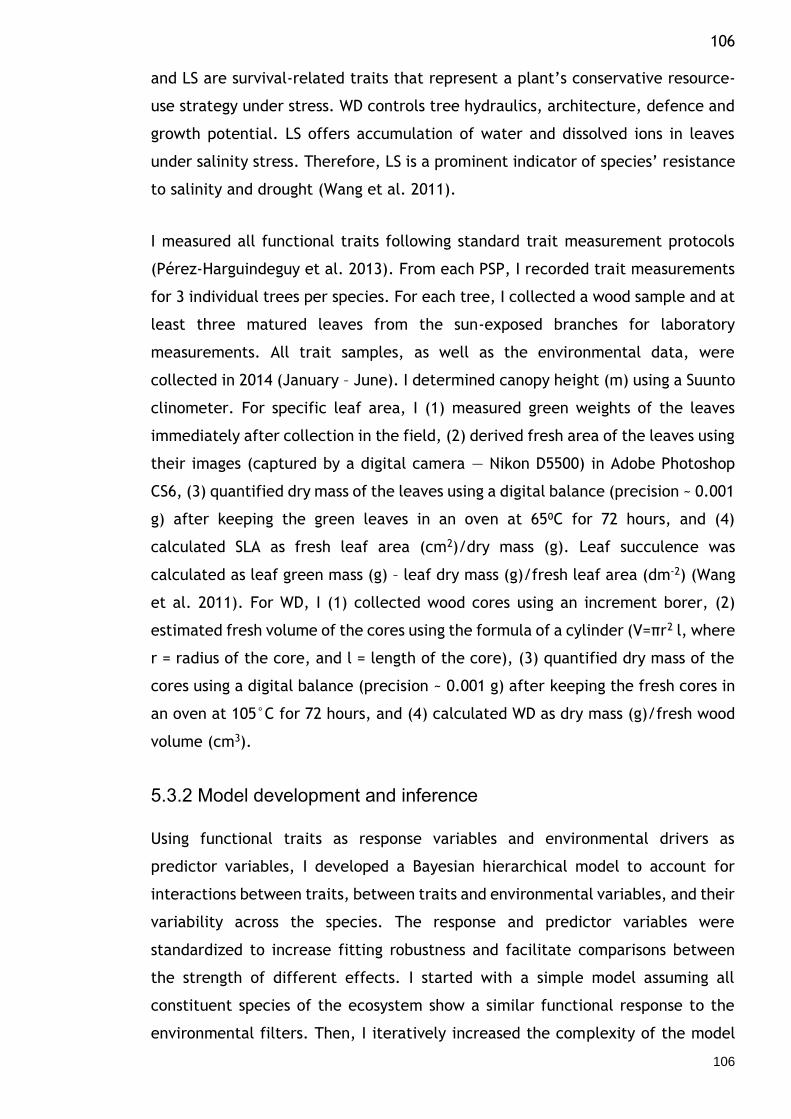
106

106

and LS are survival-related traits that represent a plant’s conservative resource-

use strategy under stress. WD controls tree hydraulics, architecture, defence and

growth potential. LS offers accumulation of water and dissolved ions in leaves

under salinity stress. Therefore, LS is a prominent indicator of species’ resistance

to salinity and drought (Wang et al. 2011).

I measured all functional traits following standard trait measurement protocols

(Pérez-Harguindeguy et al. 2013). From each PSP, I recorded trait measurements

for 3 individual trees per species. For each tree, I collected a wood sample and at

least three matured leaves from the sun-exposed branches for laboratory

measurements. All trait samples, as well as the environmental data, were

collected in 2014 (January – June). I determined canopy height (m) using a Suunto

clinometer. For specific leaf area, I (1) measured green weights of the leaves

immediately after collection in the field, (2) derived fresh area of the leaves using

their images (captured by a digital camera — Nikon D5500) in Adobe Photoshop

CS6, (3) quantified dry mass of the leaves using a digital balance (precision ~ 0.001

g) after keeping the green leaves in an oven at 65⁰C for 72 hours, and (4)

calculated SLA as fresh leaf area (cm2)/dry mass (g). Leaf succulence was

calculated as leaf green mass (g) – leaf dry mass (g)/fresh leaf area (dm-2) (Wang

et al. 2011). For WD, I (1) collected wood cores using an increment borer, (2)

estimated fresh volume of the cores using the formula of a cylinder (V=πr2 l, where

r = radius of the core, and l = length of the core), (3) quantified dry mass of the

cores using a digital balance (precision ~ 0.001 g) after keeping the fresh cores in

an oven at 105°C for 72 hours, and (4) calculated WD as dry mass (g)/fresh wood

volume (cm3).

5.3.2 Model development and inference

Using functional traits as response variables and environmental drivers as

predictor variables, I developed a Bayesian hierarchical model to account for

interactions between traits, between traits and environmental variables, and their

variability across the species. The response and predictor variables were

standardized to increase fitting robustness and facilitate comparisons between

the strength of different effects. I started with a simple model assuming all

constituent species of the ecosystem show a similar functional response to the

environmental filters. Then, I iteratively increased the complexity of the model

107

107

and compared the performance of the models using the DIC (deviance information

criterion), the Bayesian analog of the Akaike Information Criterion (Spiegelhalter

et al. 2002). I obtained posterior distributions and 95% CI (credible intervals) for

the parameters using Markov Chain Monte Carlo (MCMC) in the symbolic language

JAGS version 4.2.0 (Plummer 2015) with the ‘runjags’ interface version 2.0.2 - 8

(Denwood 2016) in software R version 3.2.3 (R Core Team 2016) (JAGS codes for

the models are in Appendix 5F). To evaluate the convergence of the two MCMC

chains, I inspected the trace plots and ensured that the potential scale reduction

factor (Gelman-Rubin statistic) for all monitored parameters was < 1.05 (Gelman

et al. 2004). For reducing the chance of any relic effects of initial values, I

discarded the first 5000 samples as burn-in and then simulated two independent

MCMC chains for 60000 iterations. Spatially explicit trait and fine-scale

environmental data on tropical and sub-tropical coastal ecosystems are

exceedingly rare (Ellison 2001). Indeed, credible previous trait and environmental

data on the Sundarbans are unavailable. Therefore, I used non-informative priors

in all models to allow data to dominate posterior parameter estimation. For

assessing the goodness-of-fit of the best model, I used R2 values from regressions

of observed vs. predicted traits.

5.3.3 Mapping traits and productivity

Using kriged surfaces (Appendix 2B, Chapter 2) of the environmental variables,

the best Bayesian model predicted functional trait distributions for the four most

prominent species (together contributed 98% of the total count). Then, using

previously derived species density maps (Fig. 2.4, Chapter 2), I averaged the

summed posterior trait values of each species weighted by their relative

abundance in each grid cell to produce community trait maps for the entire

ecosystem.

To develop whole-ecosystem biomass productivity maps, I first built species-

specific trait-based productivity models. I then linked these models with the

species traits and density maps to generate productivity predictions. I modelled

biomass productivity of individual trees (taking basal area as a proxy) as a linear

function of the functional traits using a GLM framework. I fitted all possible

candidate models with all possible combinations of predictor variables. I then used

the ‘∆AIC ≤ 2’ criterion (Burnham & Anderson 2002) to determine a set of

108

108

competing models and performed model averaging to predict plot level species-

specific productivity. Finally, I linked the GLM approach with the Bayesian mean

posterior trait surfaces and species density predictions to produce spatial

productivity maps for the whole ecosystem.

5.3.4 Forecasting traits and productivity

Salinity intrusion and siltation have strong influences on species abundances and

community composition in the Sundarbans (Chapters 2, 3 & 4). The SLR rate along

the Bangladesh coast in the 20th century was significantly higher than the global

average. The soil salinity level has already increased by 60% since 1980 due to

drop in freshwater supplies from the transboundary rivers (Aziz & Paul 2015).

Assuming continuation of such historical pressures which may further affect plant

functions via physiological stress and shifting relationships among species, I

updated the environmental and species distribution maps for five future stress

scenarios (E1 = 10, E2 = 20, E3 = 30, E4 = 40 and E5 = 50% increase in salinity and

siltation), and then used them to forecast traits and forest productivity under

these novel environments. Here, I considered E5 as the worst stress scenario for

the ecosystem by 2050.

To evaluate the robustness of these forecasts, I used samples from the joint

posterior distribution of all model parameters to simulate traits and productivity

distributions for both current and future environmental scenarios. Using these

simulations, I then mapped the posterior probability of deterioration of traits [a

decrease in growth (Height and SLA) trait values and an increase in survival (WD

and LS) trait values] and productivity at each grid cell, averaged across all grid

cells in the ecosystem, in response to each of the future stress scenarios, to

uncover the uncertainty related to my forecasts. All maps were generated using

the ‘raster’ package version 2.4 – 18 (Hijmans 2015) in R.

109

109

5.4 Results

5.4.1 Integrated modelling approach

My approach is an extension of the multivariable regression models typically used

to quantify species-habitat associations (Elith & Leathwick 2009) on the basis of

one response and multiple explanatory variables. I have augmented this approach

by allowing it to model several interdependent response variables (multiple

functional traits from multiple species), using a Bayesian hierarchical modelling

framework. This allowed a single model, fitted simultaneously to all my data, to

capture TER for 4 traits, 9 tree species, and 8 environmental drivers, while

accounting for trade-offs between different traits. Based on this inferential

template, several trait-based models (Fig. 5.3) were developed, prompted from

the viewpoints of distinct ecological hypotheses. Conducting formal model

selection among these competing versions of the model, allowed me to understand

how TER can differ across species, to generate species-specific and community-

wide trait predictions, and finally to translate these spatial predictions into spatial

forecasts of whole-ecosystem productivity.

Initially, the traits of all constituent tree species were assumed to respond

identically to environmental drivers (Model I, my base model), formulating the

hypothesis that extreme habitat filtering drives different species to show similar

functional responses in stressful environments (Weiher & Keddy 1995). This was

challenged with two alternative hypotheses. In Model II, I incorporated variability

in trait-trait relationships (TTR) for different species to capture the effects of

taxonomic variability on trait plasticity. On the other hand, to formalise the

consequences of the ‘limiting similarity’ hypothesis (MacArthur & Levins 1967;

Chesson 2000), in Model III I allowed trait responses to environmental drivers (the

trait-environment relationships, TER) to vary across species, implying that

resource partitioning and specialization (morphological or physiological) cause

different coexisting species to show dissimilar functional responses to

environmental drivers . Fig. 2 shows the relative quality of fit of the trait-based

models in terms of the deviance information criterion (DIC) (Spiegelhalter et al.

2002). Both models very strongly improved DIC over Model I (ΔDIC > 1000), with

Model III being preferred and therefore selected for future model comparisons

(but see Model VIII below).

110

110

Fig. 5.3 Flow chart of the different ecological hypotheses compared via model

selection. The different versions (I to IX) of my model were constructed by

partitioning the variability in the data in different ways to estimate trait-

environment relationships (TER) across multiple species by taking account of the

intraspecific trait-trait relationships (TTR) at various hierarchical levels. The

performances of the trait-based models were evaluated using DIC (the deviance

information criterion, whose numerical value is displayed under each model), with

arrows denoting tests made. Black arrows indicate that a new model improved DIC

over the older model, red did not, solid arrows point to new models that were

selected (the models outlined in black). Dashed arrows point to new models that

were not selected (the models outlined in red).

111

111

In extreme environments such as mangrove forests, species can usually tolerate a

certain level of stress via specialization (Feller et al. 2010). Hence, it is likely that

all species show an average functional response to environmental filters.

Nevertheless, the strength of the response around that average may vary for

different species and for different traits depending on how severe the stress

conditions are and how one trait facilitates or constrains another.

I incorporated these ecological hypotheses into models IV to VII. Model IV tested

the hypothesis that although the mangrove species differed in their response to

the environmental drivers regarding their traits, that variability is around a

common interspecific average response. This model was also strongly preferred

(ΔDIC > 500), so the next models investigated the variability around that mean.

Model V tested whether the amount of variability around the mean is different for

each trait and Model VI tested whether it is different for each environmental

driver. Model V was weakly preferred over Model IV (ΔDIC > 10), but Model VI was

very strongly preferred (ΔDIC > 1000), so Model VI was selected. Model VII then

tested whether the amount of variability around the average response is also

different for each trait (as Model V), but it was not preferred over Model VI.

This completed my analysis of the trait-environment relationships, so Model VIII

tested whether the TTR is different for each species (recapitulating Model II,

which was set aside in favour of Model III). This was still very strongly preferred

(ΔDIC > 1000), so Model IX (analogously to Model IV) tested whether, although the

TTR is different for each species, that variability is around a common interspecific

mean. Model IX was not preferred over Model VIII, indicating that there was no

common mean for the trait-trait relationships.

5.4.2 Model comparison summary

Model VIII (DIC = 48828) which is nested within Models I, III, IV and VI, was

identified as the preferred model (ΔDIC > 1000 for all models it was nested within),

showing evidence that tree species growing in a stressed ecosystem like a

mangrove forest have a typical functional response to the environmental filters

with inter-specific variability around this average, and the amount of variability

is further contingent upon the nature and magnitude of the filters. I further

112

112

observed inter-specific variability in trait-trait relationships across the species,

but the data provided no evidence for further patterns within the TTRs.

The explanatory power of the best model was high (regressions of observed vs.

predicted trait values yielded — canopy height: R2 = 0. 68, specific leaf area: R2 =

0.64, wood density: R2 = 0.94 and leaf succulence: R2 = 0.67) and plots of

predictions vs. observations indicate that the model made unbiased predictions

(Appendix 5A). The potential scale reduction factor (Gelman-Rubin statistic) for

all monitored regression parameters was < 1.05, indicating model convergence.

5.4.3 Drivers of functional traits

Soil salinity and siltation are the dominant environmental drivers that limit species

canopy height (Fig. 5.4, Table 5.1). However, the intensity of such detrimental

effects varies across the species. Salt-induced drop in canopy height is highest in

the most prominent tree species (H. fomes) of the ecosystem [posterior mean ɸ =

-0.59, 95% CI = (-0.69, -0.50)]. In contrast, increasing URP (i.e. more available

freshwater) favours height increase in many species, including the pioneer species

S. apetala [ɸ = 0.18, 95% CI = (0.05, 0.32)] and the climax H. fomes [ɸ = 0.16, 95%

CI = (0.08, 0.24)]. Soil pH, salinity, siltation, and K have limiting effects on

specific leaf area (SLA) of many species. In contrast, I identified a strong positive

response of SLA to URP and NH4 – suggesting that nitrogen-rich upstream habitats

favour plants’ resource-acquisition in tropical coastal environments.

While the growth traits (Height and SLA) show a strong negative response to

increasing salinity, siltation and pH, I discovered a clear positive response of the

survival traits (WD and LS) to these dominant environmental filters (Fig. 5.4, Table

5.1), suggesting a substantial growth-survival trade-off across the species.

Nevertheless, the strength of this positive response or positive filtering (adaptive

shifts in trait values to increase resistance to stress) varies across the species,

trait types, and environmental drivers. For example, salinity is the dominant

positive filter for H. fomes [ɸ = 0.19, 95% CI = (0.15, 0.22)], siltation for B.

sexangula [ɸ = 0.12, 95% CI = (0.04, 0.20)] and pH for X. mekongensis [ɸ = 0.11,

95% CI = (0.07, 0.15)] in terms of WD, while salinity is the predominant positive

filter for LS and the filtering is highest in X. mekongensis [ɸ = 0.34, 95% CI = (0.25,

0.43)].

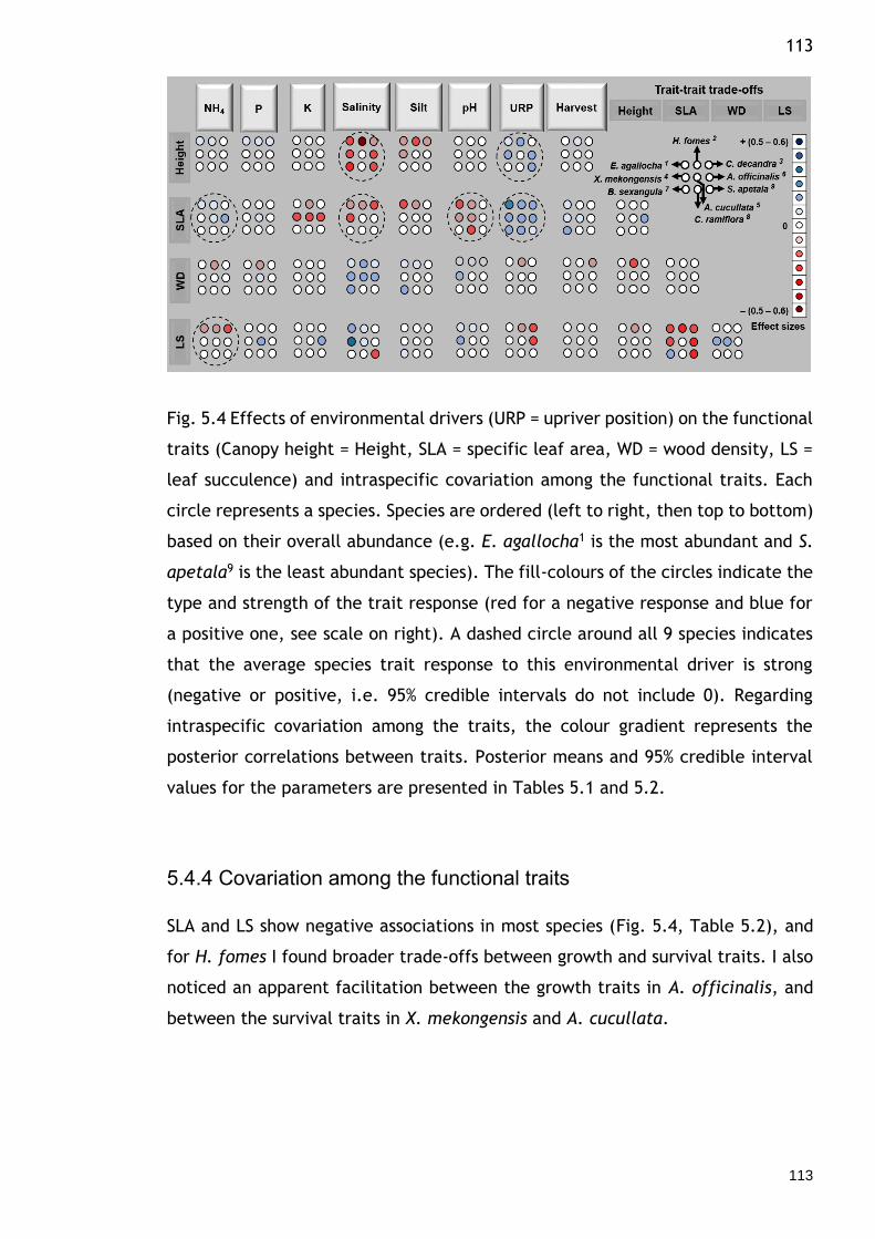
113

113

Fig. 5.4 Effects of environmental drivers (URP = upriver position) on the functional

traits (Canopy height = Height, SLA = specific leaf area, WD = wood density, LS =

leaf succulence) and intraspecific covariation among the functional traits. Each

circle represents a species. Species are ordered (left to right, then top to bottom)

based on their overall abundance (e.g. E. agallocha1 is the most abundant and S.

apetala9 is the least abundant species). The fill-colours of the circles indicate the

type and strength of the trait response (red for a negative response and blue for

a positive one, see scale on right). A dashed circle around all 9 species indicates

that the average species trait response to this environmental driver is strong

(negative or positive, i.e. 95% credible intervals do not include 0). Regarding

intraspecific covariation among the traits, the colour gradient represents the

posterior correlations between traits. Posterior means and 95% credible interval

values for the parameters are presented in Tables 5.1 and 5.2.

5.4.4 Covariation among the functional traits

SLA and LS show negative associations in most species (Fig. 5.4, Table 5.2), and

for H. fomes I found broader trade-offs between growth and survival traits. I also

noticed an apparent facilitation between the growth traits in A. officinalis, and

between the survival traits in X. mekongensis and A. cucullata.

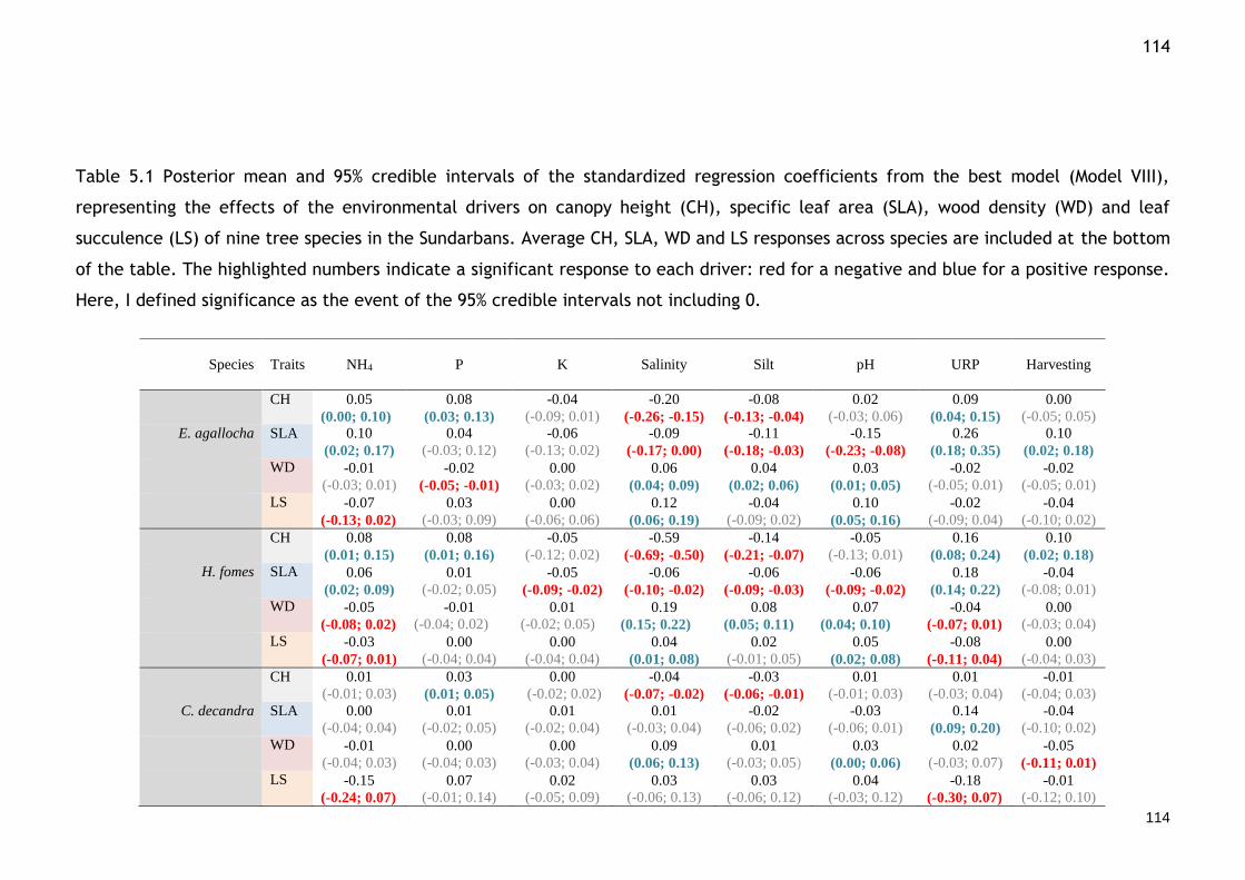
114

114

Table 5.1 Posterior mean and 95% credible intervals of the standardized regression coefficients from the best model (Model VIII),

representing the effects of the environmental drivers on canopy height (CH), specific leaf area (SLA), wood density (WD) and leaf

succulence (LS) of nine tree species in the Sundarbans. Average CH, SLA, WD and LS responses across species are included at the bottom

of the table. The highlighted numbers indicate a significant response to each driver: red for a negative and blue for a positive response.

Here, I defined significance as the event of the 95% credible intervals not including 0.

Species

Traits

NH4

P

K

Salinity

Silt

pH

URP

Harvesting

CH 0.05

(0.00; 0.10)

0.08

(0.03; 0.13)

-0.04

(-0.09; 0.01)

-0.20

(-0.26; -0.15)

-0.08

(-0.13; -0.04)

0.02

(-0.03; 0.06)

0.09

(0.04; 0.15)

0.00

(-0.05; 0.05)

E. agallocha SLA 0.10

(0.02; 0.17)

0.04

(-0.03; 0.12)

-0.06

(-0.13; 0.02)

-0.09

(-0.17; 0.00)

-0.11

(-0.18; -0.03)

-0.15

(-0.23; -0.08)

0.26

(0.18; 0.35)

0.10

(0.02; 0.18) WD -0.01

(-0.03; 0.01)

-0.02

(-0.05; -0.01)

0.00

(-0.03; 0.02)

0.06

(0.04; 0.09)

0.04

(0.02; 0.06)

0.03

(0.01; 0.05)

-0.02

(-0.05; 0.01)

-0.02

(-0.05; 0.01)

LS -0.07

(-0.13; 0.02)

0.03

(-0.03; 0.09)

0.00

(-0.06; 0.06)

0.12

(0.06; 0.19)

-0.04

(-0.09; 0.02)

0.10

(0.05; 0.16)

-0.02

(-0.09; 0.04)

-0.04

(-0.10; 0.02)

CH 0.08

(0.01; 0.15)

0.08

(0.01; 0.16)

-0.05

(-0.12; 0.02)

-0.59

(-0.69; -0.50)

-0.14

(-0.21; -0.07)

-0.05

(-0.13; 0.01)

0.16

(0.08; 0.24)

0.10

(0.02; 0.18)

H. fomes SLA 0.06

(0.02; 0.09)

0.01

(-0.02; 0.05)

-0.05

(-0.09; -0.02)

-0.06

(-0.10; -0.02)

-0.06

(-0.09; -0.03)

-0.06

(-0.09; -0.02)

0.18

(0.14; 0.22)

-0.04

(-0.08; 0.01)

WD -0.05

(-0.08; 0.02)

-0.01

(-0.04; 0.02)

0.01

(-0.02; 0.05)

0.19

(0.15; 0.22)

0.08

(0.05; 0.11)

0.07

(0.04; 0.10)

-0.04

(-0.07; 0.01)

0.00

(-0.03; 0.04)

LS -0.03

(-0.07; 0.01)

0.00

(-0.04; 0.04)

0.00

(-0.04; 0.04)

0.04

(0.01; 0.08)

0.02

(-0.01; 0.05)

0.05

(0.02; 0.08)

-0.08

(-0.11; 0.04)

0.00

(-0.04; 0.03)

CH 0.01

(-0.01; 0.03)

0.03

(0.01; 0.05)

0.00

(-0.02; 0.02)

-0.04

(-0.07; -0.02)

-0.03

(-0.06; -0.01)

0.01

(-0.01; 0.03)

0.01

(-0.03; 0.04)

-0.01

(-0.04; 0.03)

C. decandra SLA 0.00

(-0.04; 0.04)

0.01

(-0.02; 0.05)

0.01

(-0.02; 0.04)

0.01

(-0.03; 0.04)

-0.02

(-0.06; 0.02)

-0.03

(-0.06; 0.01)

0.14

(0.09; 0.20)

-0.04

(-0.10; 0.02)

WD -0.01

(-0.04; 0.03)

0.00

(-0.04; 0.03)

0.00

(-0.03; 0.04)

0.09

(0.06; 0.13)

0.01

(-0.03; 0.05)

0.03

(0.00; 0.06)

0.02

(-0.03; 0.07)

-0.05

(-0.11; 0.01) LS -0.15

(-0.24; 0.07)

0.07

(-0.01; 0.14)

0.02

(-0.05; 0.09)

0.03

(-0.06; 0.13)

0.03

(-0.06; 0.12)

0.04

(-0.03; 0.12)

-0.18

(-0.30; 0.07)

-0.01

(-0.12; 0.10)

115

115

CH 0.01

(-0.05; 0.08)

0.05

(-0.02; 0.12)

0.00

(-0.07; 0.07)

-0.15

(-0.21; -0.08)

-0.10

(-0.16; -0.03)

0.04

(-0.02; 0.10)

0.14

(0.07; 0.21)

-0.05

(-0.13; 0.02)

X. mekongensis SLA 0.05

(-0.02; 0.12)

0.04

(-0.04; 0.11)

-0.13

(-0.21; -0.05)

-0.12

(-0.20; -0.05)

-0.01

(-0.08; 0.06)

-0.09

(-0.16; -0.03)

0.15

(0.08; 0.23)

0.08

(0.01; 0.16) WD 0.01

(-0.04; 0.06)

0.03

(-0.01; 0.08)

0.01

(-0.04; 0.06)

0.13

(0.08; 0.17)

-0.01

(-0.06; 0.04)

0.11

(0.07; 0.15)

0.04

(-0.01; 0.09)

0.00

(-0.05; 0.06)

LS -0.04

(-0.13; 0.04)

0.02

(-0.06; 0.11)

0.01

(-0.07; 0.09)

0.34

(0.25; 0.43)

-0.07

(-0.15; 0.02)

0.11

(0.03; 0.19)

-0.03

(-0.12; 0.06)

-0.07

(-0.16; 0.02)

CH 0.00

(-0.06; 0.06)

0.00

(-0.06; 0.08)

-0.01

(-0.07; 0.05)

0.01

(-0.07; 0.08)

-0.06

(-0.13; 0.01)

0.00

(-0.06; 0.07)

-0.02

(-0.09; 0.04)

-0.05

(-0.12; 0.03)

A. cucullata SLA 0.10

(0.03; 0.16)

0.08 -0.11 -0.15 0.07 -0.07 0.16 0.09

(0.01; 0.16) (-0.18; -0.04) (-0.24; -0.07) (-0.01; 0.16) (-0.15; 0.00) (0.08; 0.23) (0.01; 0.18)

WD -0.03

(-0.09; 0.02)

0.09

(0.02; 0.15)

0.04

(-0.02; 0.11)

0.12

(0.04; 0.20)

0.04

(-0.03; 0.11)

-0.01

(-0.08; 0.06)

-0.04

(-0.10; 0.03)

-0.07

(-0.14; 0.01)

LS -0.05

(-0.13; 0.03)

0.16

(0.06; 0.26)

-0.01

(-0.10; 0.07)

0.11

(0.01; 0.22)

0.03

(-0.07; 0.12)

-0.03

(-0.12; 0.06)

-0.07

(-0.16; 0.02)

0.05

(-0.05; 0.15)

CH 0.05

(-0.06; 0.18)

0.04

(-0.09; 0.16)

-0.03

(-0.13; 0.08)

-0.15

(-0.30; -0.07)

0.00

(-0.11; 0.12)

0.05

(-0.08; 0.18)

0.13

(0.00; 0.26)

-0.05

(-0.17; 0.07)

A. officinalis SLA 0.15

(0.04; 0.25)

0.05

(-0.06; 0.16)

-0.11

(-0.19; -0.02)

0.08

(-0.02; 0.18)

-0.01

(-0.11; 0.08)

-0.04

(-0.16; 0.07)

0.14

(0.04; 0.24)

0.00

(-0.10; 0.10)

WD -0.01

(-0.07; 0.06)

-0.01

(-0.08; 0.06)

0.03

(-0.03; 0.09)

0.02

(-0.03; 0.07)

0.00

(-0.06; 0.05)

0.02

(-0.06; 0.10)

0.04

(-0.02; 0.10)

0.01

(-0.06; 0.08)

LS -0.05

(-0.16; 0.06)

-0.03

(-0.14; 0.09)

0.14

(0.04; 0.26)

-0.06

(-0.18; 0.05)

-0.03

(-0.13; 0.07)

0.01

(-0.11; 0.13)

-0.14

(-0.25; 0.02)

-0.02

(-0.12; 0.09)

CH -0.04

(-0.16; 0.09)

0.03

(-0.10; 0.15)

-0.05

(-0.16; 0.07)

-0.23

(-0.36; -0.09)

-0.02

(-0.12; 0.08)

0.01

(-0.10; 0.12)

0.12

(-0.01; 0.25)

-0.06

(-0.17; 0.04)

B. sexangula SLA 0.05

(-0.08; 0.17)

0.00

(-0.14; 0.13)

-0.06

(-0.18; 0.06)

0.07

(-0.11; 0.26)

0.02

(-0.11; 0.15)

-0.02

(-0.14; 0.12)

0.19

(0.04; 0.35)

0.17

(0.03; 0.32)

WD 0.02

(-0.09; 0.12)

0.07

(-0.04; 0.18)

0.06

(-0.04; 0.15)

0.11

(0.01; 0.20)

0.12

(0.04; 0.20)

0.03

(-0.06; 0.13)

0.05

(-0.07; 0.16)

-0.02

(-0.10; 0.06)

LS -0.03

(-0.13; 0.08)

0.02

(-0.08; 0.13)

0.03

(-0.06; 0.12)

0.01

(-0.08; 0.11)

0.10

(0.03; 0.18)

0.00

(-0.10; 0.09)

0.01

(-0.10; 0.14)

-0.05

(-0.11; 0.03)

CH 0.06

(-0.02; 0.15)

0.00

(-0.09; 0.11)

-0.02

(-0.13; 0.08)

0.00

(-0.15; 0.15)

0.00

(-0.06; 0.06)

0.00

(-0.10; 0.11)

-0.02

(-0.11; 0.07)

-0.03

(-0.09; 0.03)

C. ramiflora SLA 0.03

(-0.07; 0.13)

0.05

(-0.07; 0.16)

-0.09

(-0.21; 0.02)

-0.03

(-0.22; 0.15)

0.06

(-0.03; 0.15)

-0.12

(-0.24; 0.00)

0.16

(0.05; 0.27)

-0.03

(-0.10; 0.05)

116

116

WD 0.03

(-0.07; 0.12)

0.07

(-0.04; 0.19)

0.05

(-0.06; 0.16)

0.04

(-0.12; 0.22)

0.03

(-0.05; 0.10)

0.04

(-0.07; 0.15)

0.00

(-0.10; 0.10)

0.03

(-0.04; 0.10)

LS -0.06

(-0.15; 0.02)

-0.07

(-0.18; 0.03)

0.00

(-0.10; 0.10)

-0.02

(-0.16; 0.12)

-0.03

(-0.09; 0.03)

-0.01

(-0.11; 0.09)

-0.01

(-0.10; 0.08)

0.00

(-0.06; 0.05)

CH 0.08

(-0.04; 0.22)

0.11

(-0.02; 0.25)

-0.05

(-0.17; 0.05)

-0.18

(-0.33; -0.03)

0.02

(-0.13; 0.16)

-0.03

(-0.16; 0.10)

0.18

(0.05; 0.32)

-0.01

(-0.16; 0.13)

S. apetala SLA 0.02

(-0.08; 0.12)

0.07

(-0.03; 0.17)

0.01

(-0.06; 0.08)

-0.04

(-0.11; 0.04)

-0.02

(-0.14; 0.10)

-0.02

(-0.11; 0.07)

0.07

(0.01; 0.16)

0.02

(-0.11; 0.16)

WD 0.00

(-0.11; 0.11)

-0.01

(-0.12; 0.09)

-0.01

(-0.08; 0.07)

0.04

(-0.04; 0.11)

0.03

(-0.08; 0.15)

0.03

(-0.06; 0.13)

0.00

(-0.08; 0.08)

-0.02

(-0.15; 0.12)

LS -0.08

(-0.20; 0.04)

0.07

(-0.04; 0.19)

0.04

(-0.05; 0.13)

-0.14

(-0.25; -0.03)

0.10

(-0.03; 0.23)

-0.03

(-0.15; 0.08)

-0.02

(-0.12; 0.09)

-0.02

(-0.15; 0.13)

Average effect CH 0.03

(-0.02; 0.08)

0.04

(-0.01; 0.09)

-0.03

(-0.07; 0.02)

-0.11

(-0.19; -0.03)

-0.04

(-0.09; 0.01)

0.01

(-0.05; 0.06)

0.07

(0.02; 0.13)

-0.02

(-0.07; 0.04)

SLA 0.05

(0.01; 0.10)

0.03

(-0.02; 0.09)

-0.06

(-0.11; -0.01)

-0.02

(-0.10; 0.05)

-0.01

(-0.06; 0.04)

-0.06

(-0.11; -0.01)

0.13

(0.07; 0.20)

0.03

(-0.02; 0.09)

WD 0.00

(-0.05; 0.04)

0.02

(-0.03; 0.07)

0.02

(-0.02; 0.06)

0.05

(-0.02; 0.13)

0.03

(-0.02; 0.08)

0.03

(-0.01; 0.08)

0.00

(-0.05; 0.06)

-0.01

(-0.06; 0.04)

LS -0.06

(-0.11; 0.01)

0.03

(-0.03; 0.08)

0.02

(-0.03; 0.07)

0.03

(-0.05; 0.11)

0.01

(-0.04; 0.06)

0.02

(-0.03; 0.08)

-0.05

(-0.11; 0.01)

-0.02

(-0.07; 0.04)

117

117

Table 5.2 Intraspecific covariation among the traits. Blue numbers indicate significant positive and red numbers indicate significant

negative posterior correlations between traits. Here, I defined significance as the event of the 95% credible intervals not including 0.

Species

Height – SLA

Height - WD

Height - LS

SLA - WD

SLA - LS

WD - LS

E. agallocha -0.03

(- 0.11; 0.04)

-0.06

(-0.18; 0.04)

0.03

(-0.06; 0.10)

-0.01

(-0.11; 0.07)

-0.15

(-0.25; -0.06)

0.06

(-0.04; 0.13)

H. fomes 0.05

(-0.03; 0.13)

-0.19

(-0.33; -0.09)

-0.1

(-0.22; -0.01)

-0.02

(-0.14; 0.08)

-0.27

(-0.45; -0.14)

0.09

(-0.02; 0.17)

C. decandra -0.06

(-0.24; 0.07)

-0.10

(-0.29; 0.04)

-0.03

(-0.17; 0.08)

-0.08

(-0.26; 0.05)

-0.19

(-0.35; -0.07)

0.06

(-0.06; 0.14)

X. mekongensis -0.03

(-0.17; 0.06)

-0.08

(-0.26; 0.04)

-0.06

(-0.19; 0.02)

0.05

(-0.08; 0.15)

-0.20

(-0.36; -0.08)

0.13

(0.03; 0.21)

A. cucullata -0.03

(-0.28; 0.12)

-0.04

(-0.3; 0.11)

-0.07

(-0.30; 0.08)

-0.17

(-0.47; 0.01)

-0.05

(-0.27; 0.08)

0.18

(0.02; 0.27)

A. officinalis 0.14

(0.02; 0.21)

0.02

(-0.20; 0.13)

-0.07

(-0.23; 0.03)

-0.11

(-0.44; 0.09)

-0.29

(-0.60; -0.11)

0.17

(-0.04; 0.28)

B. sexangula 0.01

(-0.15; 0.11)

-0.10

(-0.46; 0.09)

0.01

(-0.32; 0.17)

-0.07

(-0.29; 0.06)

0.19

(0.05; 0.26)

0.22

(-0.06; 0.35)

C. ramiflora 0.00

(-0.54; 0.21)

-0.02

(-0.62; 0.21)

-0.12

(-1.0; 0.16)

-0.10

(-0.62; 0.12)

-0.05

(-0.67; 0.18)

-0.18

(-0.95; 0.09)

S. apetala 0.08

(-0.24; 0.21)

0.05

(-0.29; 0.19)

-0.1

(-0.40; 0.06)

-0.08

(-0.93; 0.18)

-0.30

(-0.90; -0.01)

0.24

(-0.10; 0.36)

118

118

5.4.5 Trait and productivity maps

My integrated Bayesian approach offers species-specific as well as community-

wide spatial trait predictions under current and future stress scenarios regarding

salinity intrusion and siltation, and link them with the trait-based productivity

models to forecast ecosystem productivity. It further evaluates the robustness of

such forecasts by propagating parameter uncertainty through sampling from the

joint posterior distribution of all model parameters and simulating traits and

productivity distributions for both current and future stress scenarios.

Spatial maps (Fig. 5.5) revealed that the most productive tree communities are

currently distributed in the freshwater dominated eastern and northern

Sundarbans. If historical increases in salinity and siltation are maintained, my

model predicts a significant productivity loss over the entire ecosystem under all

future stress scenarios (10, 20, 30, 40 and 50% increase in salinity and siltation)

(Fig. 5.6A) although there is the possibility of local productivity gains in a few of

the communities, particularly under the least stress future scenarios (Appendix

5B). The worst stress scenario (a 50% rise in salinity and siltation) is predicted to

push the ecosystem to lose 30% of its current total productivity by 2050 (Fig. 5.6A).

119

119

Fig. 5.5 Current status (first column) and worst-case scenario for the year 2050

(second column), of community-weighted posterior mean of tree canopy height

(Height), specific leaf area (SLA), wood density (WD), leaf succulence (LS) and

forest productivity (FP) in the Sundarbans world heritage ecosystem. Uncertainties

related to these forecasts are mapped as the posterior probability of deterioration

(see section 5.3.4 and Appendices 5B & 5C) in the third column. Deterioration is

considered to be a decrease in productivity and growth trait (Height and SLA)

values, or an increase in survival trait (WD and LS) values.

120

120

Fig. 5.6 Bar charts show the response of the ecosystem to each of five future stress

scenarios, E1 to E5, representing a 10% to 50% increase in both salinity and

siltation for the whole Sundarbans ecosystem by 2050. (A) shows mean percentage

decline in whole ecosystem productivity; (B) shows mean percentage decline in

community canopy height (CH) and community specific leaf area (SLA), and

increase in community wood density (WD) and community leaf succulence (LS);

121

121

(C) shows mean percentage decline in CH and SLA, and increase in WD and LS for

four prominent mangrove tree species under five future stress scenarios. The

species short-hands are Excoecaria agallocha (Ea), Ceriops decandra (Cd),

Xylocarpus mekongensis (Xm) and Heritiera fomes (Hf). Decreases in CH and SLA

and increases in LS and WD are considered to be deteriorations in the traits.

The eastern and northern regions currently support the tallest mangrove

communities. However, if the habitat degradation trend is continued, it is highly

likely that these tallest communities will turn into dwarf communities, following

an average of 36% height loss by 2050 (Fig. 5.6B, Appendix 5C). In turn, I predict

a community-wide increase in the values of LS (14%) and WD (5%) – indicating

highly plastic responses of the mangrove species to ensure efficient water use and

mechanical support under the extreme stress scenarios, by 2050. Community SLA

showed more stable patterns between time-points.

My species-specific trait predictions (Figs. 5.7, 5.8, 5.9 & 5.10) further determined

that although every constituent species of the ecosystem will lose height under

the future stress scenarios, the loss will be substantially higher for the climax

species H. fomes (52%) by 2050 (Fig. 5.7, Appendix 5D). The increase in WD (9%)

is also highest for this species. In turn, the disturbance specialist species — C.

decandra - which is expected to undergo ecosystem-wide range expansion by 2050

(Appendix 5E), loses the least amount of height and SLA, compared to others.

122

122

Fig. 5.7 Current status (first column) and worst-case scenario for the year 2050

(second column), of posterior mean of tree canopy height for four prominent

mangrove tree species in the Sundarbans world heritage ecosystem. Uncertainties

related to these forecasts are mapped as the posterior probability of a decrease

in canopy height in the third column.

123

123

Fig. 5.8 Current status (first column) and worst-case scenario for the year 2050

(second column), of posterior mean of tree SLA for four prominent mangrove tree

species in the Sundarbans world heritage ecosystem. Uncertainties related to

these forecasts are mapped as the posterior probability of a decrease in SLA in

the third column.

124

124

Fig. 5.9 Current status (first column) and worst-case scenario for the year 2050

(second column), of posterior mean of tree wood density for four prominent

mangrove tree species in the Sundarbans world heritage ecosystem. Uncertainties

related to these forecasts are mapped as the posterior probability of an increase

in wood density in the third column.

125

125

Fig. 5.10 Current status (first column) and worst-case scenario for the year 2050

(second column), of posterior mean of tree leaf succulence for four prominent

mangrove tree species in the Sundarbans world heritage ecosystem. Uncertainties

related to these forecasts are mapped as the posterior probability of an increase

in leaf succulence in the third column.

126

126

5.5 Discussion

Primary production in tropical forest ecosystems is affected by the complex

interactions between species’ functional traits and the scene set by different

environmental drivers. These are interconnected processes that collectively

(through forest species composition and individual species function) determine

fundamental functional aspects of the entire forest, such as its productivity.

Looking at subsets of this causal network (e.g. statistical relationships between

single traits and the environment) can only reveal part of the biological signal in

the data. By underrepresenting the complexity of the connections between traits,

species and environment (a challenge known as the “fourth-corner problem”), any

predictive model of future forest dynamics stands to suffer from increased

imprecision and by failing to propagate parameter uncertainty through to the

prediction stages we risk ascribing unjustifiable confidence in any such

predictions. In this paper, I have developed an analytical approach that follows a

more holistic view of forest ecosystems, both by developing a model as complex

as the data would support and by fully propagating parameter uncertainty into the

predictions. This approach resolves the “fourth-corner problem”, contributes to

the clarification of different theoretical hypotheses about how complex forest

ecosystems function, uncovers the environmental drivers of functional traits, and

generates predictions about how traits and forest productivity will be affected by

the environmental change in the future.

My integrated Bayesian approach allowed different ecological hypotheses to be

tested in a single analysis simultaneously using all available data. In extreme

environments, such as the tropical inter-tidal zones, tree communities may

comprise functionally redundant species (Ricotta et al. 2016). Therefore, the

studied species might have shown homogeneous functional responses to the

stressors. Model I (Fig. 5.3) which represents this expectation (i.e. the ‘habitat

filtering’ hypothesis (Weiher & Keddy 1995)) received the least support in my

analyses. Rather, I found better support for Model III (representing the ‘limiting

similarity’ hypothesis (MacArthur & Levins 1967; Chesson 2000)), suggesting that

resource partitioning and specialization cause different coexisting mangrove

species to show disparate functional trait responses to the environmental drivers.

However, Model VIII, which considers both the ‘habitat filtering’ (by assuming that

all species show an average functional trait response to the environmental drivers)

127

127

and the ‘limiting similarity’ (by assuming that the amount of variability around

the average functional trait response depends on the nature and magnitude of the

drivers) hypotheses, received the most support from my data. This suggests that

habitat filtering and limiting similarity jointly explain mangroves’ trait responses

to the environment.

Applying my approach to the dynamic Sundarbans ecosystem, I determined

salinity, siltation, pH and upriver position as the key drivers governing plants’ trait

responses (Fig. 5.4, Table 5.1). Further, I discovered diverging trait responses

among the species and the strength of such responses to the environmental drivers

was found to vary across the trait categories. For example, among the traits,

height was more affected by salinity than the other drivers and the magnitude of

the effect was significantly higher on the climax species H. fomes than the

generalists — E. agallocha and C. decandra. These species-specific differences in

canopy height (and for other traits) responses could be related to the variability

in water stress, nutritional imbalance, and salt stress that the species experience

under variable saline environments (Rasool et al. 2013).

Simultaneous plastic decreases in growth traits (Height and SLA) and plastic

increases in survival traits (WD and LS) along the soil salinity, siltation and pH

gradients, suggest conservative resource-use (low resource acquisition and

turnover rates, and slow growth rates) as the dominant ecological strategy in many

species to ensure their long-term survival under unfavourable environments

(Rosado et al. 2016). The growth and survival traits showed opposing responses to

increasing upriver-position (i.e. more available freshwater), suggesting that the

same species can increase resource acquisition and growth under benign

environmental conditions.

My model predicts an ecosystem-wide productivity loss under all future stress

scenarios and forecasts a 30% loss of its current total productivity under the

highest stress scenario by 2050 (Fig. 5.6A, Appendix 5B). This productivity loss is

mainly associated with the community-wide decreases (36%) in height, by 2050

(Fig. 5.6B, Appendix 5C). Trait maps (Fig. 5.5) reveal that community SLA and WD

show more stable patterns between the stress scenarios. This could be the result

of turnover in species composition rather than stasis in stress conditions (Appendix

5E). For example, while the climax species — H. fomes (medium SLA and high WD)

128

128

— is projected to lose most of its suitable habitat by 2050, both generalist — E.

agallocha (high SLA and low WD) — and disturbance specialist species — C.

decandra (low SLA and high WD) — are likely to replace most of the degraded

habitats and are projected to undergo ecosystem-wide range expansions. My

species-specific predictions further uncovered spatial variability in plastic

responses of the traits under projected stress conditions. I found that, under

increasing stress, every species will lose canopy height and SLA, but the loss will

be substantially higher for the climax species H. fomes (52% height and 16% SLA

loss by 2050) (Fig. 5.6C, Appendix 5D) which is in agreement with the previous

results that the species has narrower salt-tolerance than the generalists because

of its limited ability to balance water and salt uptake (Das 1999). Plastic increases

in conservative trait values (WD and LS) were also predicted to be highest for this

species, implying maximum stress on the species contributing the most biomass.

While my approach incorporated multiple species, intra-specific variations in

traits, in common to other existing approaches (Dolédec et al. 1996; Legendre et

al. 1997; Lavorel et al. 2007; Pollock et al. 2012; Jamil et al. 2012; Jamil et al.

2013; Dray et al. 2014; Brown et al. 2014; Warton et al. 2015), it did not consider

competitive interactions between species. Species-species interactions can lead

to trait divergence (i.e. limited trait similarity) or sometimes trait convergence

when traits have a strong influence on the competitive ability of the coexisting

species which in turn may affect the species composition and biomass productivity

in forest communities. However, my empirical inferences can inform more

mechanistic models of tree dynamics (Purves et al. 2008; Grueters et al. 2014;

Chauvet et al. 2017) that will better capture tree interaction dynamics.

In addition, several fundamental unknowns might also interfere with my forecasts.

The first is the climate- or local stress-induced trait acclimation and adaptation

that could potentially affect the accuracy of the projected trait values and

productivity. However, variability in acclimation potential among different tree

species and different trait types have yet to be discovered in mangrove ecosystems

and elsewhere (Van Bodegom et al. 2014). The second unknown is the degree to

which environment–trait relationships and trait–trait interactions will remain the

same under future climatic and stress conditions (i.e. whether they undergo

abiotic/biotic filtering).

129

129

Another area of improvement is to consider traits that directly measure the fitness

or reproductive success of individual species. The fitness of individual species

depends mainly on its ability to use and conserve resources or to tolerate abiotic

and biotic stresses (Grime 2001). Therefore, the ideal trait for predicting species,

community and ecosystem level productivity under variable stress scenarios is one

whose function directly reflects the physiological or mechanical mechanisms

controlling resource acquisition or conservation or stress tolerance in primary

producers. Physiological (or hard) traits such as the relative growth rate of plants

(RGR) which directly measures biomass allocation in plants, offer such an

opportunity. However, their quantification is costly and time demanding and

cannot be measured for large numbers of species in many regions of the world

(Weiher et al. 1999). All the traits in this study are ‘soft’ or ‘morphological’ traits.

The functional interpretations of them are rather indirect which might have

resulted in increased uncertainty in parameter estimations and spatial predictions

of traits and productivity. The positive side of including them is that they are

available for all tree species whatever the scale is and closely represent many

‘hard’ traits. For example, I considered SLA as a surrogate of RGR as species with

high SLA-leaves have higher RGR (Pérez-Harguindeguy et al. 2013). Future models

incorporating available ‘hard’ traits or a mixture of ‘soft’ and ‘hard’ traits may

offer a better mechanistic understanding of trait-environment relationships, and

more accurate predictions of shifts in trait range under future environmental

conditions and resulting consequences for ecosystem functioning.

My integrated approach not only advances our understanding of previously

unknown functional trait responses of threatened taxa such as mangroves under

variable stress conditions, but also provides forest managers a much-needed

functional basis to tailor science-driven management and conservation actions

particularly for conservation priority areas like the Sundarbans. Inadequate

knowledge of how different mangrove species respond in dynamic coastal

environments has previously led to unsuccessful conservation efforts in many

tropical regions (Lewis 2005), including the Sundarbans (Islam et al. 2014).

Therefore, determining the environmental drivers that limit mangroves’ growth

and survival is crucial before designing and implementing habitat restoration and

reforestation programs. For example, my finding that soil salinity, alkalinity and

siltation are the most limiting environmental drivers of mangroves’ primary

130

130

growth and resource acquisition, especially for the climax species, can target the

selection of species and sites for future reforestation and restoration initiatives.

My finding that currently the productivity hotspots are confined to the hyposaline

eastern and northern regions in the Sundarbans and the projected 30% decline in

productivity, lends strong support for immediate habitat enhancement programs

(e.g. river dredging for increasing freshwater flows and for reducing silt

deposition) in the eastern and northern regions. Most importantly, the

productivity maps can be important tools for implementing the United Nations

REDD+ (Reduced Emissions from Deforestation and Degradation) initiatives and

guiding national strategy while negotiating for payments for ecosystem services

(Rahman et al. 2015).

The application of my proposed approach is not limited to mangrove forests rather

this is a generalizable foundation for powerful modelling of trait-environment

linkages under changing climate and for predicting their consequences on

ecosystem functions and services in other forest ecosystems of the world (e.g.

boreal, temperate, and other tropical forests). The increasing availability of

spatially explicit global datasets for plant functional traits (Kattge et al. 2011),

species distributions (Hudson et al. 2014), and high-resolution environmental

layers (Shangguan et al. 2014) provide opportunities for such applications,

especially within dynamic global vegetation models (Scheiter et al. 2013).

131

131

5.6 Conclusions

This integrated Bayesian approach provides the foundations for trait-based

predictions in plant ecology through simultaneously modelling trait-trait and trait-

environment correlations (for multiple traits, species, and environmental drivers)

at organismal, community and ecosystem levels, thus resolving many fundamental

methodological problems of the existing ordination/permutation and univariate

approaches, and bridges community, ecosystem ecology, and functional

biogeography. These novel developments allow us to (1) integrate fundamental

ecological hypotheses into the model building process, (2) quantify the strength

of the trait-environment relationships, (3) identify the degree of intraspecific

covariation among multiple traits, (4) predict species-specific and community-

level trait distributions with accurate estimates of uncertainty, and (5) forecast

whole-ecosystem productivity under future environmental conditions. Applying

this approach to the Sundarbans, I discovered (1) joint effects of habitat filtering

and limiting similarity in shaping trait responses to environment with parallel

contribution of intraspecific variability in trait-trait interactions, (2) substantial

intraspecific trade-offs among the functional traits in many tree species, (3)

serious detrimental effects of increasing salinity, siltation and soil alkalinity on

functional traits associated with plants’ resource acquisition and growth, (4)

plastic enhancement of traits related to stress tolerance, indicative of plants

prioritizing survival over growth, and (5) ecosystem-wide drop in biomass

productivity under all anticipated stress scenarios with an average of 30%

productivity loss by 2050 in the worst scenario. These findings advance our

understandings on how species living in stressed ecosystems respond to

environmental change and provide policymakers and managers with a much-

needed functional basis for developing strategic approaches and setting targets

for forest conservation, restoration, and ecosystem management. Because of its

high computational efficiency, my integrated approach is applicable to any forest

ecosystem across broad global scales, to predict shifts in ecosystem functioning

and services under a rapidly changing climate.

132

132

Chapter 6 . General Discussion

6.1 An overview of my thesis findings

My overall aim of this thesis was to understand mangroves’ habitat requirements

and spatial distributions, to explore spatio-temporal patterns and drivers of

Sundarbans’ biodiversity, and to develop an integrated approach for predicting

species trait responses and forest productivity under changing environments. In

Chapter 2, using GAMs on mangrove abundances, I determined habitat preferences

and spatial distributions of the four major mangrove tree species. The climax

species H. fomes showed a strong negative response to salinity and human

harvesting. H. fomes and X. mekongensis preferred upstream habitats while the

remaining species preferred downstream to intermediate-stream areas. The

magnitude of responses to nutrients, elevation, and the biotic interaction term

varied between species. Spatial maps show that the established protected area

network (PAN) does not cover the density hotspots of any of the tree species.

In Chapter 3, using long-term mangrove tree data collected at four historical time

points (1986, 1994, 1999 and 2014), I uncovered the spatial heterogeneity in

alpha, beta, and gamma diversity and temporal dynamics in species abundances,

geographic range, and composition in the existing ecological zones (hypo-, meso-

, and hypersaline) of the Sundarbans. Here, I also developed regional biodiversity

maps to pinpoint the historical and current biodiversity hotspots and to specify

the areas that experienced shifts in species composition over time. I found that

the hyposaline zone supported the most diverse and heterogeneous communities

(in terms of species composition) at all historical time points. In contrast, the

hypersaline zone comprised the least diverse and most homogeneous

communities. Most importantly, I detected a clear trend of decreasing

heterogeneity in the mangrove communities of all ecological zones since 1986,

providing a strong signal for ecosystem-wide biotic homogenization. Biodiversity

maps revealed that the established PAN neither supported the historical

biodiversity hotspots nor the existing hotspots. They further identified the

western and southern hypersaline zones as the areas that have experienced the

greatest species compositional shifts (biotic differentiation) since 1986.

133

133

In Chapter 4, using GAMs on tree count, environmental and historical disturbance

data, my objectives were to determine the key drivers for different aspects

(alpha, beta and gamma) of mangrove biodiversity and to develop habitat data-

driven baseline biodiversity maps for the Sundarbans. I found historical tree

harvesting, siltation, disease and soil alkalinity as the key stressors that negatively

influenced the diversity (alpha) and distinctness (beta) of the mangrove

communities. In contrast, species diversity increased along the downstream –

upstream, and riverbank – forest interior gradients, suggesting the late

successional upstream and forest interior communities are more diverse than the

early successional downstream and riverbank communities. Like the species

density hotspots, the existing PAN does not cover the remaining biodiversity

hotspots.

In Chapter 5, I developed an integrated Bayesian modelling approach to quantify

trait-environment correlations for multiple traits, species, and environmental

drivers simultaneously while accounting for the intraspecific variation in traits.

The approach thus resolves the ‘fourth-corner problem’ (Legendre et al. 1997)

and provides a foundation for mechanistic trait-based predictions in plant ecology.

Applying this approach on the Sundarbans, I found (1) combined effects of habitat

filtering and limiting similarity in shaping trait responses to environment with

parallel contribution of intraspecific variability in trait-trait interactions, (2)

substantial intraspecific trade-offs among the functional traits in many tree

species, (3) serious detrimental effects of increasing salinity, siltation and soil

alkalinity on plant primary growth, and parallel plastic enhancement of traits

related to stress tolerance and (4) ecosystem-wide drop in biomass productivity

under all anticipated stress scenarios.

Although each data chapter had separate aims and answered specific questions,

they mainly covered three central themes: habitat preferences of mangroves,

spatio-temporal patterns and drivers of mangrove biodiversity, and species trait

responses to environmental drivers. I collect the insights for each of the themes

below and then briefly discuss the practical implications of my findings,

limitations and potential areas for future improvements.

134

134

6.1.1 Habitat preferences of mangroves

Habitat suitability analyses in Chapter 2 uncovered that multiple environmental

drivers (i.e. salinity, upriver position, harvesting, nutrients) simultaneously

influence spatial distributions of mangroves. This contrasts with the common

mangrove-centric assumption that only a few abiotic stressors (e.g. temperature,

tidal waves etc.) shape mangrove distributions in the harsh tropical inter-tidal

zones (Ellison 2001).

All the mangroves showed steep responses to increasing salinity although the

magnitude of the responses clearly varied between species. H. fomes showed a

strong negative response while the remaining species showed clear positive

responses. These results are in agreement with previous studies (Ball 2002;

Dangremond et al. 2015) reporting that differential salt tolerance and salinity

optima among mangrove species contribute to spatial variability in mangrove

populations in tropical coastal areas.

Changes in river hydro-geomorphological features along the downstream-

upstream gradient alter habitat qualities which in turn may cause spatial

variability in species distributions (Angiolini et al. 2011). Likewise, I found

differential habitat preferences of the Sundarbans’ mangroves along the

downstream-upstream gradient. Most suitable habitats of H. fomes and X.

mekongensis are now located in the upstream areas although records show their

widespread distributions over the entire forest in the 19th century (Gopal &

Chauhan 2006). This shift in habitat preferences may be related to riparian

degradation through hydrological modification (e.g. a 60% drop in the freshwater

flow in the Sibsha and Posur river system), increasing river-bank erosion and

siltation which have modified the fluvial geomorphology of the waterbodies in the

Sundarbans (Wahid et al. 2007).

Before the Bangladeshi government enforced a full logging ban in 1989 (Sarker et

al. 2011), the Sundarbans was managed for sustainable timber production in the

Pakistani (1948 — 1970) and the British (1600 — 1947) regimes (Ghosh et al. 2015).

Despite the enforcement of a full logging ban, tree harvesting by local

communities is common (Iftekhar & Saenger 2008). My results showed that past

harvesting has had substantial negative effects on the populations of H. fomes, X.

135

135

mekongensis and C. decandra. Siddiqi (2001) reported intensive past harvesting of

C. decandra by local communities for fuelwood, and selective logging of H. fomes

and X. mekongensis by the BFD for timber supply. Interestingly, E. agallocha

showed the opposite pattern: a clear trend of population increase in the highly-

exploited areas in the past. Frequent tropical cyclones, past industrial and illegal

logging, and tree mortality have resulted in large as well as small forest gaps in

the Sundarbans and the size of open areas has been increasing by 0.05% each year

(Iftekhar & Islam 2004). E. agallocha is a salt tolerant fast producing species that

can easily colonise open and degraded habitats (Harun-or-Rashid et al. 2009). I

assume that these conditions may favour E. agallocha to increase its density even

in the H. fomes and X. mekongensis dominated stands. Increasing dominance of

E. agallocha in the previously H. fomes dominated stands, and increasing coverage

of mono-specific E. agallocha stands - 0.69% per year during 1981-1997 (Iftekhar

& Saenger 2008) - provide support for my assumption.

In common with other terrestrial plant communities, nutrient availability is

recognized as a major driver for spatial variability in abundance, composition and

productivity in mangrove communities (Feller et al. 2010). Often, mangrove soils

are poor in nutrients and nutrient availability is irregularly driven by a complex

interaction between abiotic and biotic variables (Reef et al. 2010). Mangroves

have developed several nutrient conservation strategies (e.g. resorption of

nutrients before leaf shedding, evergreenness) to maintain growth and

development under such conditions. Moreover, mangroves can show high plasticity

in their ability to opportunistically exploit nutrients when they become available

depending on their physiological requirements, thus for a specific nutrient the

responses of different species may vary (Reef et al. 2010). Likewise, I found that

the magnitude of response to nutrients varied between mangroves in the

Sundarbans.

H. fomes prefers NH4 rich habitats while the others can grow abundantly in NH4-

poor habitats. Terrestrial plants put considerable respiration effort to uptake and

assimilate N and those are well adapted to the efficient uptake and assimilation

of NH4 require much less respiration efforts (i.e. less metabolic cost) compared to

uptake and assimilation of other N forms (Reef et al. 2010). This indicates that H.

fomes might have increased its capacity to efficiently utilize NH4 as the main N

136

136

source for saving metabolic cost under increasing salinity stress in the Sundarbans.

Conversely, the apparent preference of salt-tolerant mangroves for NH4-poor

habitats may be related to their preference for other forms of N, or they may

suffer from NH4 toxicity (Kronzucker et al. 1997). Soil P is a key constraint for

forest productivity in the tropics (Baribault et al. 2012). Interestingly, in the

Sundarbans, all the mangroves show a preference for habitats with relatively

lower P availability. K is a key soil macro-nutrient that can modulate salinity-

induced drought stress by improving the water uptake and retention capacity of

plants (Sardans & Peñuelas 2015). The salt-tolerant species such as E. agallocha,

C. decandra and X. mekongensis maintain high abundances in the K-rich habitats

(north-western Sundarbans). Fe and Mg are required in minute quantities for

successful mangrove growth because of their roles in metabolic and physiological

processes (Alongi 2010). Responses to Fe substantially varied between species.

Interestingly, mangroves mostly accumulate Fe in roots (Alongi 2010). H. fomes

and X. mekongensis have extensive aerial root system (i.e. pneumatophores). E.

agallocha has spreading surface roots, and C. decandra has extensive knee roots

(Siddiqi 2001). These differential rooting structures may be related to diverse Fe

use efficiency in the mangroves. H. fomes’s higher preference range for Mg than

X. mekongensis may be related to the distribution and chemical properties of the

source rock material, the weathering process, and salinity levels which control

the availability of Mg to mangrove plants (Gransee & Führs 2013).

The above responses to nutrients indicate that the mangroves of Sundarbans may

be highly plastic in their ability to utilize nutrients (i.e. withstand low-nutrient

conditions, but able to exploit high levels of nutrients when other stresses are

withdrawn). Future research is required to understand the plasticity levels in

different mangroves, and their nutrient acquisition, and conservation strategies

under different stress scenarios (e.g. salt stress and flooding).

Species distribution maps reveal that currently, the eastern region of the

Sundarbans supports the remaining H. fomes hotspots, the north-western region

supports the E. agallocha hotspots, the western and southern regions support the

C. decandra hotspots, and few specific areas in the northern (Kalabogi and Koyra)

and north-western (Koikhali) regions support the X. mekongensis hotspots. H.

fomes was the most abundant species both in the Bangladesh and Indian parts of

137

137

the Sundarbans just 200 years ago (Siddiqi 2001). Currently, the species is at the

elevated risk of extinction in the Indian Sundarbans. Historical obstruction of

freshwater influx from the Ganga-Bhagirathi-Hooghly river system, salinity

intrusion, deposition of industrial effluents, and aquaculture expansion which

have gradually transformed it into world’s one of the most degraded mangrove

ecosystems (Kathiresan 2010). The more stress tolerant species C. decandra is now

the climax species in the heavily degraded Indian Sundarbans.

Most of the world’s H. fomes trees are now restricted only to the less saline

eastern region of the Bangladesh Sundarbans. Evidence of widespread distribution

of H. fomes in the western region (currently, the hypersaline zone) in the past

(Gopal & Chauhan 2006), suggests historical range contraction of the species in

the Bangladesh Sundarbans. C. decandra has already replaced a substantial

amount of H. fomes range: 0.08% year-1 during the period 1981—1997 (Iftekhar &

Saenger 2008). Gopal & Chauhan (2006) have documented an annual replacement

of about 0.4% of the total forest area by C. decandra. Therefore, the Indian

Sundarbans case should be taken as a warning regarding the future availability of

suitable habitats for H. fomes and other salt-intolerant (freshwater loving) species

in the Bangladesh Sundarbans.

6.1.2 Spatio-temporal patterns and drivers of mangrove biodiversity

Species diversity, composition, abundance, and geographic range of the

mangroves have substantially changed in the Sundarbans over the last three

decades (Chapter 3). This finding is consistent with recent remote-sensing

technique-based studies (Giri et al. 2007; Mukhopadhyay et al. 2015; Ghosh et al.

2015) reporting species and vegetation cover changes in the Sundarbans since the

1980s. Chapter 4 further determined the drivers for spatial variability in diversity

and species composition.

At all historical time points (1986, 1994, 1999 and 2014), the hyposaline mangrove

communities remained the most diverse (alpha) while the hypersaline

communities remained the least diverse. Chapter 2 has already revealed

widespread distributions of the facultative halophyte H. fomes in the less saline

nitrogen rich upstream areas that also allow co-existence of other salt-intolerant

non-halophytes (Siddiqi 2001). In turn, two obligate halophytes: E. agallocha and

138

138

C. decandra showed super-dominance in the highly saline down – intermediate

stream habitats. Therefore, the relatively higher diversity in the hyposaline

communities may be closely related to suitable habitat conditions that supported

historical coexistence of both facultative (e.g. H. fomes) as well as other

opportunistic non-halophytes.

Surprisingly, in the last 15 years, alpha diversity sharply increased in the

communities of the southern meso- and western hypersaline areas. My temporal

beta diversity analyses detected that these areas have also experienced radical

shifts in species composition over the 28 years. Salinity fluctuation is highest in

these areas and often the salinity level remains high for longer, inhibiting the

regeneration process and inducing disease outbreaks in many salt-intolerant

species, including H. fomes (Ghosh et al. 2016). Habitat-based biodiversity models

in Chapter 4 uncovered that historical harvesting, increasing siltation, salinity, pH

and community size (dominance of generalists) have strong negative effects on

alpha diversity while increasing upstream and forest interior environment have

strong positive effects on alpha diversity as well as the gamma diversity. Chapter

4 further showed that increasing salinity could promote increasing heterogeneity

in the communities. This is due to the increasing colonization success of the

opportunistic stress-tolerant species (e.g. E. agallocha and C. decandra) in the

degraded saline soils in the Sundarbans (Iftekhar & Saenger 2008; Aziz & Paul 2015;

Mukhopadhyay et al. 2015) with associated population declines and range

contraction of many stress-intolerant species (Chapter 3). Therefore, range and

population expansion of the stress-tolerant species and range contraction and

population loss of the stress-intolerant species under increasing salt stress,

harvesting, siltation, and soil alkalinity could be the possible mechanisms that

resulted in sudden alpha diversity increase and alteration to the species

composition (particularly in the southern meso- and western hypersaline

communities) over the 28 years.

A disproportionate expansion of generalist (or invasive) species relative to

specialist endemics which results in reduced distinctness in natural communities

is the key mechanism responsible for biotic homogenization (Olden 2006). Chapter

3 revealed (1) increasing similarity (decreasing distinctness) among mangrove

communities since 1986, (2) range expansion of the widespread stress-tolerant

139

139

species (e.g. E. agallocha and C. decandra) and range contraction of the local

endemics, (3) increasing abundance of the stress-tolerant species and decreasing

abundance of the stress-intolerant endemics including the climax H. fomes, and

(4) local extinction of many rare mangrove species. These findings strongly comply

with the basic assumptions of the biotic homogenization theory (McKinney &

Lockwood 1999; Olden & Poff 2003; Olden & Rooney 2006).

Chapter 4 determined historical tree harvesting, increasing disease prevalence,

siltation, soil alkalinity, nutrient toxicity as the key stressors responsible for

increasing similarity among mangrove communities. Since the construction of the

Farakka dam in the upstream, both water and soil salinity have been increasing in

the Sundarbans (Mirza 1998; Wahid et al. 2007). The average soil salinity has

already increased by 60% since 1980 (Aziz & Paul 2015). As a result, hyposaline

areas are transforming into mesosaline areas and mesosaline areas are

transforming into hypersaline areas (Ghosh et al. 2016). Despite the ongoing ban

on logging (Sarker et al. 2011), opportunistic tree felling is common (Iftekhar &

Islam 2004). This ongoing transformation in habitat conditions coupled with forest

exploitation and sea level rise may seriously alter the current biodiversity and

species composition in the Sundarbans. Biodiversity maps in Chapter 3 revealed

that the spatial coverage of the heterogeneous (distinct) communities gradually

declined at all historical time points since 1986. Together, Chapter 3 and Chapter

4 maps confirm that the most diverse and the most distinct communities are now

confined to a specific area (Kalabogi) in the Sundarbans while the rest of the

ecosystem looks homogeneous in terms of species composition, suggesting further

degradation and forest exploitation may transform these remaining biodiversity

hotspots into species-poor homogeneous patches.

6.1.3 Quantifying species trait responses to environmental drivers

A variety of approaches — the CWM (Lavorel et al. 2007), the fourth corner

correlation (Legendre et al. 1997; Dray & Legendre 2008), the multivariate RLQ

(Dolédec et al. 1996; Dray et al. 2014), and the more recent regression approches

(Pollock et al. 2012; Jamil et al. 2012; Jamil et al. 2013; Brown et al. 2014;

Warton et al. 2015) — are used to disentangle the link between species traits and

environmental drivers (known as ‘the fourth-corner problem’ in community

ecology) and to model the link for predicting species, community and ecosystem

140

140

responses under future environmental scenarios. The survival of a species in a

specific environment is controlled by how its functional traits (morphological or

physiological or anatomical) respond to multiple environmental stressors and how

the trait themselves interact (Verberk et al. 2013). Therefore, the interplay

between multiple plant functional traits, multiple species and multiple

environmental drivers may collectively influence species abundance, community

composition and ecosystem productivity.

However, current trait-based approaches often look at species, traits and the

environment in a fragmented way, and frequently deal with the effect of single

(or sometimes several) environmental driver on individual species traits without

considering the complex interactions between multiple traits of multiple

competing species under a dynamic environment. These shortcomings raise serious

concerns (Webb et al. 2010; Verberk et al. 2013; Funk et al. 2017) about how

precisely the existing approaches will forecast species, community and ecosystem

responses under future environmental conditions. Therefore, we need an

integrated quantitative approach that represents the complexity of the

connections between traits, species and environmental drivers while developing a

predictive model of future forest dynamics. In Chapter 5, I proposed such an

integrated approach that models trait-environment relationships for multiple

traits, species, and environmental drivers simultaneously while accounting for

intraspecific trait variation. In this way, this novel approach resolves the long-

lasting ‘fourth-corner problem’ problem and contributes to the clarification of

different theoretical assumptions about how complex forest ecosystems function,

determines the environmental drivers of functional traits, and makes predictions

about how traits and forest productivity will be affected by the future changes in

the environment.

A common assumption in mangrove literature is that a few strong environmental

gradients (such as salinity and tidal inundation) shape structural and functional

properties of mangrove forests, and regular species sorting along these gradients

are responsible for poor species diversity and relatively homogeneous species

composition at least at a regional scale (Farnsworth 1998). This reflects the

‘habitat filtering’ theory (Weiher & Keddy 1995), a widely tested theory for many

taxa in diverse ecosystems. An alternative assumption also exists saying fine-scale

141

141

variation in habitat conditions in the dynamic inter-tidal zones may cause

variability in species composition and functioning which reflects the ‘limiting

similarity’ theory (MacArthur & Levins 1967; Chesson 2000). My proposed

integrated Bayesian approach allowed these ecological hypotheses to be tested in

a single analysis simultaneously using all available data and revealed that habitat

filtering and limiting similarity together explain mangroves’ trait responses to the

environment with strong influences of within-species variability in trait-trait

relationships.

Applying my approach to the Sundarbans, I found severe detrimental effects of

increasing salinity, siltation and soil alkalinity, and a significant positive effect of

increasing upriver position (i.e. more available freshwater) on height and SLA,

indicating trees living in the freshwater-dominated upstream areas have higher

resource acquisition and growth rates than those living in the alkaline and highly

silted hypersaline environments. In parallel, a plastic enhancement of survival

traits — WD and LS — was common in many species. Higher LS is a common

adaptation mechanism in many plants to ensure water use efficiency under

extended stress (e.g. drought, salinity etc.) periods (Wang et al. 2011). Denser

wood confers mechanical stiffness to trees growing under heavily silted saline

soils, but needs more biomass investment and is therefore costlier to construct

per unit of stem height (Feller et al. 2010). This extra resource investment of trees

in structural support leaves less available resource in a plant body that could be

used for fitness purposes (such as photosynthesis and primary growth),

representing the growth-survival trade-off (Lawson et al. 2015). My integrated

approach identified such trade-off in the most abundant species of the ecosystem

— H. fomes.

Contrary to the common assumption that mangroves show homogeneous

functional responses under stress as they are believed to share evolutionarily

convergent traits (Farnsworth 1998), I discovered plastic trait responses among

the species and the strength of such responses to the environmental drivers varied

for both growth and survival traits. For example, while salinity has its greatest

negative effect on the height of H. fomes and its greatest positive effect on X.

mekongensis LS, pH has no significant effect on the height of any of the species.

But increasing pH significantly affects the SLA of all species with maximum

142

142

negative effect on E. agallocha. These findings indicate that multiple

environmental drivers simultaneously act on traits, and plastic responses of traits

and trait-trait interactions differ among different species which might collectively

determine the growth and survival of species.

My model predicts that currently the most productive mangrove tree communities

are distributed in the freshwater-dominated hyposaline habitats (eastern and

northern regions) while the most unproductive communities are distributed in the

highly silted hypersaline habitats (western and south-western regions) in the

Sundarbans. Biomass productivity in tree communities is closely connected with

the community-wide trait values (Grime 1998; Diaz et al. 2007). Hence, higher

biomass productivity in the hyposaline habitats than the silted hypersaline

habitats might be related to relatively higher community-wide height and SLA

(which together may facilitate greater light capture, photosynthetic rates and net

carbon gain) and relatively lower community-wide wood density (resulting in

higher stem hydraulic conductivity, photosynthetic carbon gain and lower

construction costs per wood volume) in the hyposaline habitats. The relatively

nutrient-rich soils (particularly, nitrogen) and biodiverse hyposaline habitats

(Chapters 3 & 4) might also contribute to greater biomass productivity in these

regions because plants can grow faster in nutrient-rich soils (Pastor et al. 1984;

Prado-Junior et al. 2016) and a higher diversity of species offers efficient use of

available resources because of higher niche differentiation and interspecific

facilitation (Tilman 1999).

Chapter 2 and Chapter 4 showed strong negative effects of increasing salinity and

siltation on endemic species abundances and diversity in the Sundarbans.

Projected sea level rise (32 cm by 2050) along the Bangladesh coasts (Karim &

Mimura 2008) and other aspects of climate change such as increased temperature,

monsoon flooding and extended dry season are likely to severely degrade the

Sundarbans ecosystem with subsequent effects on species traits and forest

productivity. My model-based forecasts show that the biomass productivity of the

ecosystem is likely to drop under all projected stress scenarios (10, 20, 30, 40 and

50% increase in salinity and siltation) with a maximum of 30% whole-ecosystem

productivity loss under the worst stress scenario by 2050. This productivity loss is

mainly related to a significant reduction in community-wide height (36% by 2050)

143

143

because of change in species compositiojn and an ecosystem-wide population

increase and range expansions of the less-biomass contributing generalists (such

as E. agallocha and C. decandra (Chapters 3 and 5). My species-specific predictions

further revealed that every species would lose canopy height and SLA and gain WD

and LS under all projected stress conditions, but the rate of loss might vary

between the species. Most importantly, the height loss and WD gain could be

greatest in the most biomass-contributing species H. fomes, suggesting maximum

stress on that globally endangered species.

6.2 Practical applications

Chapter 2 specified the environmental requirements of the threatened mangroves

and produced species distribution maps. Chapter 5 uncovered how functional

responses of different mangrove species vary along the environmental gradients

and generated species- and community-level trait maps under current and future

environmental conditions. Together, these species-centric and trait-based

findings, can help forest managers selecting suitable species and sites for

replanting. For example, a significantly stronger negative response of H. fomes

abundance and canopy height to increasing salinity compared to the responses of

the generalists (E. agallocha and C. decandra) imply for choosing relatively benign

upstream habitats for H. fomes replanting and planting the generalists or salt-

tolerant early-successional species (e.g. S. apetala) in the highly degraded barren

areas for initial site stabilization.

The process of biotic homogenization has been underway in the Sundarbans

resulting in spatial contraction of diverse and distinct mangrove communities in

the Sundarbans (Chapter 3). Biodiversity maps revealed that both the historical

and contemporary biodiversity hotspots were located at the northern (specifically

the Kalabogi region) hyposaline habitats that support the unique association of X.

mekongensis and H. fomes, the two species most at risk of local and global

extinction. Therefore, future conservation and protection initiatives should

primarily focus on these surviving hotspots because further habitat degradation

and exploitation of these threatened species may push them to the brink of

extinction.

144

144

Establishing coastal protected areas has been common practice in the tropics to

conserve forest resources and to offer social and economic benefits to the forest-

dependent communities (de Almeida et al. 2016). A PAN (the largest coastal PAN

in the world) is also operational in the Sundarbans to confirm completely

undisturbed habitats for plants and animals. My species density maps (Chapter 2),

biodiversity maps (Chapters 3 and 4) and the forest productivity maps (Chapter 5)

have shown that the established PAN does not cover the species density,

biodiversity, and forest productivity hotspots. Therefore, this thesis advocate for

bringing these hotspots under protected area management to ensure the long-

term conservation of the many threatened species living there.

Historical harvesting had a significant negative effect on the abundance of most

of the mangroves (Chapter 2) and appeared responsible for the diminishing

distinctness of the mangrove communities (Chapter 4). Many rare and endemic

plant species including the climax H. fomes have faced range contractions or local

extirpations over the last three decades (Chapter 3). Although logging has been

legally prohibited since 1989 (Sarker et al. 2011), opportunistic harvesting of

valuable timber-yielding species (mostly X. mekongensis and H. fomes) by

poachers is common (Iftekhar & Saenger 2008). The BFD has ratified the

‘Bangladesh Biodiversity Act 2017’ to reduce biodiversity loss and recently

initiated the SMART patrol management system to stop this illegal practice in the

Sundarbans. My species density and biodiversity maps can guide these valuable

protection and monitoring initiatives through tracking individual species

populations and community-level diversity changes or predicting changes and

recognizing habitats or species that may be affected by future human

interventions.

Both mangrove enhancement (reducing biotic and abiotic stresses that caused

mangroves’ population decline) and mangrove restoration (restoring specific areas

where certain mangrove species previously existed) initiatives are regularly taken

in the tropical coastal regions to enhance species resistance and resilience to

climate change and to offset predicted losses from climate change impacts (Lewis

2005). However, inadequate understanding of which environmental drivers

regulate mangroves abundances, composition and functions have resulted in

unsuccessful mangrove enhancement and restoration projects in many countries

145

145

(Lewis 2005) including the Sundarbans (Islam et al. 2014). This thesis determined

the key drivers responsible for spatial variations in mangrove distributions,

diversity, and functions in the Sundarbans. For example, salinity and historical

harvesting predominantly affect H. fomes abundance, siltation, disease, historical

harvesting and pH affect the diversity and distinctness of the mangrove

communities, and soil salinity, alkalinity, and siltation act simultaneously to limit

mangroves’ resource acquisitive traits and overall ecosystem productivity. These

novel habitat and functional insights and the spatial maps of species, biodiversity,

traits, and forest productivity can guide the future mangrove enhancement and

restoration initiatives in the Sundarbans.

Also, my proposed integrated approach (Chapter 5) for quantifying trait-

environment relationships and predicting ecosystem properties (such as

productivity) is not restricted to mangroves. It can be readily applied to any other

forest ecosystems of the world (e.g. boreal, temperate, and other tropical forests)

to address various management and conservation issues therein.

Finally, based on the findings in Chapters 2 ─ 5, this thesis recommends to ─

• Replant globally endangered H. fomes and locally threatened X.

mekongensis in less saline upstream habitats (Chapter 2).

• Focus protection actions (e.g. regular patrolling, increase the number of

resource protection officers and rangers) on the endangered (e.g., H.

fomes) as well as the rare endemics (e.g. C. ramiflora, C. manghas and A.

cucullata) whose populations and geographic ranges have substantially

declined in recent times (Chapter 3).

• Take extreme caution while implementing nutrient enrichment programs

because the mangroves of the Sundarbans may suffer from nutrient toxicity

in highly silted hypersaline habitats (Chapter 4).

• Focus future conservation and protection initiatives primarily on the

surviving biodiversity hotspots located in the northern Sundarbans

(Chapters 3 and 4).

146

146

• Extend or establish new protected areas for immediate protection of the

remaining species density, biodiversity and forest productivity hotspots in

the Sundarbans (Chapters 2, 3, 4 and 5).

• Take initiatives to test the suitability of interventions such as river dredging

to increase the freshwater supply in the Sundarbans to reduce the salinity

stress on tree growth and productivity of the ecosystem.

6.3 Limitations and future directions

The HSMs of the mangroves (Chapter 2) are data-driven correlative models that

do not necessarily reflect the causal relationships between species and

environmental conditions. Here, the fitted response curves for each mangrove

species only described how its densities were correlated with multiple predictors

within their observed environmental ranges. Since these predictors include

proxies for competition, these curves do not necessarily reveal the physiological

limits (i.e. the fundamental niche) of the mangroves. Future studies may

overcome the above limitations by developing mechanistic models (Dormann et

al. 2012) that relate physiological (or morphological) traits with habitat data to

translate species – environment interaction into fitness components (e.g. survival,

growth, reproduction etc.) for predicting species distribution across space and

time (Kearney & Porter 2009).

Because of low prevalence ratio (many zeroes) in the dataset, I could not develop

HSMs for the 15 rare mangrove species. Future studies can usefully extend their

sampling efforts beyond the existing PSP network to record these rare mangroves.

As previous environmental data were unavailable, I used ordinary kriging to

generate biodiversity (alpha, beta and gamma) maps for four historical time points

(Chapter 3). Because this direct interpolation approach does not accommodate

environmental and biotic predictors, it might have increased prediction

uncertainty (Miller et al. 2007). Chapter 4 used both environmental and biotic

variables to model and to produce spatial biodiversity maps. Here, the habitat-

based models showed better predictive ability than the covariate-free direct

interpolation approach. However, small differences between the approaches in

147

147

terms of predictive accuracy demonstrates the utility of direct interpolation

approaches when environmental data are unavailable.

Anthropogenic pressures, sea level rise, and natural calamities may alter the

already stressed habitats of the mangroves with subsequent changes in the salinity

and nutrient levels. Therefore, the mangrove HSMs (Chapter 2), the biodiversity

models (Chapter 3) and the trait-based models (Chapter 5) should be updated with

new environmental data. I could not incorporate hydroperiod data into my models

due to their unavailability which might have affected the predictive accuracy of

the models. Hydroperiod (the frequency, duration and depth of tidal inundation)

directly regulates salinity and nutrient dynamics in mangrove forest floors, thus,

influences mangrove regeneration and growth (Crase et al. 2013). The anticipated

sea-level rise in the Bangladesh coast may considerably alter the Sundarbans’

regional hydrology. Therefore, future studies should include plot level

hydroperiod information when they become available.

Similar to the existing trait-based approaches (Dolédec et al. 1996; Legendre et

al. 1997; Lavorel et al. 2007; Pollock et al. 2012; Jamil et al. 2012; Jamil et al.

2013; Dray et al. 2014; Brown et al. 2014; Warton et al. 2015), the proposed

Bayesian integrated approach (Chapter 5) did not include species-species

interactions. Such inclusion might have contributed to better parameter estimates

as species composition and functions of plant communities can be mediated by

competition-induced shifts in traits i.e. trait divergence or convergence (Grime

2006; Mayfield & Levine 2010). Nevertheless, my modelling framework can be

easily extended to include the abundance of one tree species as a covariate for

another (Chapter 2).

I used easily measurable morphological (‘soft’) traits that are proxies of ‘hard’

traits (for example, SLA as a proxy of the relative growth rate of plants, Pérez-

Harguindeguy et al. 2013). ‘Hard’ traits directly influence the resource acquisition

or conservation or stress tolerance hence the fitness in primary producers (Grime

2001). Therefore, future models incorporating important ‘hard’ traits may offer a

better mechanistic understanding of how species, community and ecosystem will

respond to future environmental changes.

148

148

6.4 Conclusions

Global climate change, local habitat modifications, and human interventions are

acting simultaneously to push the mangrove biome to the brink of extinction. Yet,

we have a restricted understanding of how these global and local drivers regulate

mangrove populations, composition and functions in space and time. Such

fundamental knowledge gaps have obstructed the management and conservation

programs across the tropics but particularly in the Sundarbans — a global priority

ecosystem that is being impacted simultaneously by climate change, habitat

modifications and multiple types of human exploitation. Therefore, the main

motivation behind this thesis was to fill such knowledge gaps and to provide a

spatially explicit baseline for managing and conserving mangrove populations,

biodiversity, and ecosystem functioning in the threatened Sundarbans.

Moving from autecology to synecology and applying species-centric to trait-centric

approaches on mangrove field data, this thesis (i) advances our understanding on

previously unknown habitat preferences of mangroves and their spatial

distributions, (ii) explores spatial and temporal dynamics and the determinants of

mangrove biodiversity, and (iii) develops a novel integrated approach that resolves

the “fourth-corner problem” and contributes to the clarification of different

theoretical assumptions about species functional responses under stress, specifies

the environmental drivers of functional traits, and generates predictions about

how traits and forest productivity will be affected by future changes in

environmental conditions.

The findings of this thesis have important management and conservation

implications. Results on species habitat suitability and functional trait analyses,

together, can guide regional forest managers in selecting suitable species and sites

for replanting. The ecosystem-wide decline of diversity and distinctness of the

mangrove communities and range contractions or local extirpations of many rare

and endemic species over the last three decades suggest for extending the existing

protected area network as they currently do not cover the remaining species

density and biodiversity hotspots. In addition to providing a basis for designing

spatially explicit and cost effective field inventories and monitoring programs, my

species, biodiversity, traits, and forest productivity maps can guide the forest

protection, habitat enhancement and restoration initiatives in the Sundarbans.

149

149

Finally, this thesis points for possible improvements in several areas. The

correlative HSMs and the habitat-based biodiversity models can be updated to

mechanistic models by incorporating physiological or morphological traits for

predicting species distribution across space and time. The integrated approach for

quantifying trait – environment relationships could be extended to account for

species-species interactions and should incorporate physiological traits when

available. The HSMs, the biodiversity models and the trait-based models should

be updated time to time with new environmental data to account for the spatial

and temporal changes in the habitat conditions. Given the roles of hydroperiod in

modulating habitat conditions that in turn may limit or favour plant growth and

development, I suggest the inclusion of hydroperiod in future models.

150

150

Reference List

de Almeida, L.T. et al., 2016. Evaluating ten years of management effectiveness

in a mangrove protected area. Ocean & Coastal Management, 125, pp.29–

37.

Alongi, D.M., 2014. Carbon Cycling and Storage in Mangrove Forests. Annual

Review of Marine Science, 6(1), pp.195–219.

Alongi, D.M., 2010. Dissolved iron supply limits early growth of estuarine

mangroves. Ecology, 91(11), pp.3229–3241.

Alongi, D.M., 2015. The Impact of Climate Change on Mangrove Forests. Current

Climate Change Reports, 1(1), pp.30–39.

Anderwald, P. et al., 2012. Seasonal trends and spatial differences in marine

mammal occurrence in Broadhaven Bay, north-west Ireland. Journal of the

Marine Biological Association of the United Kingdom, 92(08), pp.1757–1766.

Angiolini, C. et al., 2011. Using Multivariate Analyses to Assess Effects of Fluvial

Type on Plant Species Distribution in a Mediterranean River. Wetlands,

31(1), pp.167–177.

Austin, M.., 2002. Spatial prediction of species distribution: an interface

between ecological theory and statistical modelling. Ecological Modelling,

157(2-3), pp.101–118.

Aziz, A. et al., 2013. Prioritizing threats to improve conservation strategy for the

tiger Panthera tigris in the Sundarbans Reserve Forest of Bangladesh. Oryx,

47(4), pp.1–9.

Aziz, A. & Paul, A., 2015. Bangladesh Sundarbans: Present status of the

environment and Biota. Diversity, 7(3), pp.242–269.

Ball, M.C., 2002. Interactive effects of salinity and irradiance on growth:

implications for mangrove forest structure along salinity gradients. Trees,

16(2-3), pp.126–139.

151

151

Banerjee, K., Gatti, R.C. & Mitra, A., 2017. Climate change-induced salinity

variation impacts on a stenoecious mangrove species in the Indian

Sundarbans. Ambio, 46(4), pp.492–499.

Barbier, E.B. et al., 2011. The value of estuarine and coastal ecosystem services.

Ecological Monographs, 81(2), pp.169–193.

Baribault, T.W., Kobe, R.K. & Finley, A.O., 2012. Tropical tree growth is

correlated with soil phosphorus, potassium, and calcium, though not for

legumes. Ecological Monographs, 82(2), pp.189–203.

Barton, K., 2015. MuMIn: Multi-model inference. R package version 1.10.5.

Barwell, L.J., Isaac, N.J.B. & Kunin, W.E., 2015. Measuring β - diversity with

species abundance data T. Coulson, ed. Journal of Animal Ecology, 84(4),

pp.1112–1122.

Berger, U. et al., 2008. Advances and limitations of individual-based models to

analyze and predict dynamics of mangrove forests: A review. Aquatic

Botany, 89(2), pp.260–274.

Biswas, S.R. et al., 2007. Do invasive plants threaten the Sundarbans mangrove

forest of Bangladesh? Forest Ecology and Management, 245(1-3), pp.1–9.

Blasco, F., Aizpuru, M. & Gers, C., 2001. Depletion of the mangroves of

Continental Asia. Wetlands Ecology and Management, 9, pp.245–256.

Van Bodegom, P.M., Douma, J.C. & Verheijen, L.M., 2014. A fully traits-based

approach to modeling global vegetation distribution. Proceedings of the

National Academy of Sciences of the United States of America, 111(38),

pp.13733–8.

Bonthoux, S., Baselga, A. & Balent, G., 2013. Assessing community-level and

single-species models predictions of species distributions and assemblage

composition after 25 years of land cover change. PloS one, 8(1), p.e54179.

ter Braak, C.J.F., Cormont, A. & Dray, S., 2012. Improved testing of species

152

152

traits–environment relationships in the fourth-corner problem. Ecology,

93(7), pp.1525–1526.

ter Braak, C.J.F., Peres-Neto, P. & Dray, S., 2017. A critical issue in model-

based inference for studying trait-based community assembly and a

solution. PeerJ, 5, p.e2885.

Bremner, J.M. & Breitenbeck, G.A., 1983. A simple method for determination of

ammonium in semimicro-Kjeldahl analysis of soils and plant materials using

a block digester . Soi. Sci. Plant Anal., 14, pp.905–913.

Brown, A.M. et al., 2014. The fourth-corner solution - using predictive models to

understand how species traits interact with the environment N. Yoccoz, ed.

Methods in Ecology and Evolution, 5(4), pp.344–352.

Bunt, J., 1996. Mangrove Zonation: An Examination of Data from Seventeen

Riverine Estuaries in Tropical Australia. Annals of Botany, 78(3), pp.333–

341.

Bunt, J.S. & Stieglitz, T., 1999. Indicators of mangrove zonality  : the Normanby

river , N. E. Australia. Mangrove and Salt Marshes, 3(2), pp.177–184.

Burnham, K.P. & Anderson, D.R., 2002. Model Selection and Multimodel

Inference: a Practical Information-theoretic Approach, 2nd edn. Springer-

Verlag, New York,

De Cáceres, M. et al., 2012. The variation of tree beta diversity across a global

network of forest plots. Global Ecology and Biogeography, 21(12), pp.1191–

1202.

Cadotte, M.W., Carscadden, K. & Mirotchnick, N., 2011. Beyond species:

Functional diversity and the maintenance of ecological processes and

services. Journal of Applied Ecology, 48(Wilkins 2009), pp.1079–1087.

Carrasquilla-Henao, M. & Juanes, F., 2017. Mangroves enhance local fisheries

catches: a global meta-analysis. Fish and Fisheries, 18(1), pp.79–93.

153

153

Chain-Guadarrama, A. et al., 2017. Potential trajectories of old-growth

Neotropical forest functional composition under climate change. Ecography,

(February), pp.1–14.

Chauvet, M. et al., 2017. Using a forest dynamics model to link community

assembly processes and traits structure S. Russo, ed. Functional Ecology,

38(1), pp.42–49.

Chave, J. et al., 2009. Towards a worldwide wood economics spectrum. Ecology

Letters, 12(4), pp.351–366.

Chen, Y. & Ye, Y., 2014. Effects of Salinity and Nutrient Addition on Mangrove

Excoecaria agallocha R. P. Niedz, ed. PLoS ONE, 9(4), p.e93337.

Chesson, P., 2000. Mechanisms of Maintenance of Species Diversity. Annual

Review of Ecology and Systematics, 31(2000), pp.343–358.

Chowdhury, M.Q., Kitin, P., et al., 2016. Cambial dormancy induced growth rings

in Heritiera fomes Buch.- Ham.: a proxy for exploring the dynamics of

Sundarbans, Bangladesh. Trees, 30(1), pp.227–239.

Chowdhury, M.Q. et al., 2008. Nature and periodicity of growth rings in two

Bangladeshi mangrove species. IAWA Journal, 29(3), pp.265–276.

Chowdhury, M.Q., De Ridder, M. & Beeckman, H., 2016. Climatic Signals in Tree

Rings of Heritiera fomes Buch.-Ham. in the Sundarbans, Bangladesh N. K. P.

Kumaran, ed. PLOS ONE, 11(2), p.e0149788.

Connell, J.H., 1978. Diversity in Tropical Rain Forests and Coral Reefs. Science,

199(4335), pp.1302–1310.

Crase, B. et al., 2013. Hydroperiod is the main driver of the spatial pattern of

dominance in mangrove communities. Global Ecology and Biogeography,

22(7), pp.806–817.

Crase, B. et al., 2015. Modelling both dominance and species distribution

provides a more complete picture of changes to mangrove ecosystems under

154

154

climate change. Global Change Biology, 21(8), pp.3005–3020.

Da Cruz, C.C. et al., 2013. Distribution of mangrove vegetation along inundation,

phosphorus, and salinity gradients on the Bragança Peninsula in Northern

Brazil. Plant and Soil, 370(1-2), pp.393–406.

Dangremond, E.M., Feller, I.C. & Sousa, W.P., 2015. Environmental tolerances of

rare and common mangroves along light and salinity gradients. Oecologia,

179(4), pp.1187–1198.

Danielsen, F. et al., 2005. The Asian tsunami: a protective role for coastal

vegetation. Science (New York, N.Y.), 310(October), p.643.

Daru, B.H. et al., 2013. A Global Trend towards the Loss of Evolutionarily Unique

Species in Mangrove Ecosystems. PloS one, 8(6), p.e66686.

Das, S., 1999. An adaptive feature of some mangroves of Sundarbans, West

Bengal. Journal of Plant Biology, 42(June), pp.109–116.

Dasgupta, N. et al., 2012. Protein and enzymes regulations towards salt

tolerance of some Indian mangroves in relation to adaptation. Trees, 26(2),

pp.377–391.

Denwood, M.J., 2016. runjags  : An R Package Providing Interface Utilities, Model

Templates, Parallel Computing Methods and Additional Distributions for

MCMC Models in JAGS. Journal of Statistical Software, 71(9), pp.1–25.

De Deurwaerder, H. et al., 2016. How are anatomical and hydraulic features of

the mangroves Avicennia marina and Rhizophora mucronata influenced by

siltation? Trees - Structure and Function, 30(1), pp.35–45.

Devictor, V. et al., 2010. Spatial mismatch and congruence between taxonomic,

phylogenetic and functional diversity: The need for integrative conservation

strategies in a changing world. Ecology Letters, 13(8), pp.1030–1040.

Diaz, S. et al., 2007. Incorporating plant functional diversity effects in

ecosystem service assessments. Proceedings of the National Academy of

155

155

Sciences, 104(52), pp.20684–20689.

Díaz, S. et al., 2015. The global spectrum of plant form and function. Nature,

529(7585), pp.167–171.

Dolédec, S. et al., 1996. Matching species traits to environmental variables: a

new three-table ordination method. Environmental and Ecological

Statistics, 3(2), pp.143–166.

Donato, D.C. et al., 2011. Mangroves among the most carbon-rich forests in the

tropics. Nature Geoscience, 4(4), pp.1–5.

Dormann, C.F. et al., 2012. Correlation and process in species distribution

models: bridging a dichotomy. Journal of Biogeography, 39(12), pp.2119–

2131.

Dormann, C.F., 2007. Promising the future? Global change projections of species

distributions. Basic and Applied Ecology, 8(5), pp.387–397.

Dray, S. et al., 2014. Combining the fourth-corner and the RLQ methods for

assessing trait responses to environmental variation. Ecology, 95(1), pp.14–

21.

Dray, S. & Legendre, P., 2008. Testing the species traits environment

relationships: The fourth-corner problem revisited. Ecology, 89(12),

pp.3400–3412.

Duke, N.C. et al., 2007. A World Without Mangroves? Science, 317(5834), p.41b–

42b.

Duke, N.C., 2001. Gap creation and regenerative processes driving diversity and

structure of mangrove ecosystems. Wetlands Ecology and Management,

9(3), pp.267–279.

Duke, N.C., Ball, M.C. & Ellison, J.C., 1998. Factors Influencing Biodiversity and

Distributional Gradients in Mangroves. Global Ecology and Biogeography

Letters, 7(1), p.27.

156

156

Duke, N.C., Ball, M.C. & Ellison, J.C., 1998. Factors Influencing Biodiversity and

Distributional Gradients in Mangroves. Global Ecology and Biogeography

Letters, 7(1), p.27.

Elith, J. & Leathwick, J.R., 2009. Species Distribution Models: Ecological

Explanation and Prediction Across Space and Time. Annual Review of

Ecology, Evolution, and Systematics, 40(1), pp.677–697.

Ellison, A.M., 2001. Macroecology of mangroves: large-scale patterns and

processes in tropical coastal forests. Trees, 16(2-3), pp.181–194.

Ellison, A.M., Farnsworth, E.J. & Merkt, R.E., 1999. Origins of mangrove

ecosystems and the mangrove biodiversity anomaly. Global Ecology and

Biogeography, 8(2), pp.95–115.

Ellison, A.M., Mukherjee, B.B. & Karim, A., 2000. Testing patterns of zonation in

mangroves: Scale dependence and environmental correlates in the

Sundarbans of Bangladesh. Journal of Ecology, 88(5), pp.813–824.

Eskildsen, A. et al., 2013. Testing species distribution models across space and

time: high latitude butterflies and recent warming. Global Ecology and

Biogeography, 22(12), pp.1293–1303.

Farnsworth, E.J., 1998. Issues of Spatial, Taxonomic and Temporal Scale in

Delineating Links between Mangrove Diversity and Ecosystem Function.

Global Ecology and Biogeography Letters, 7(1), p.15.

Faucon, M.-P., Houben, D. & Lambers, H., 2017. Plant Functional Traits: Soil and

Ecosystem Services. Trends in Plant Science, 22(5), pp.385–394.

Feller, I.C. et al., 2010. Biocomplexity in Mangrove Ecosystems. Annual Review

of Marine Science, 2(1), pp.395–417.

Ferrier, S. & Guisan, A., 2006. Spatial modelling of biodiversity at the

community level. Journal of Applied Ecology, 43(3), pp.393–404.

Flowers, T.J., Galal, H.K. & Bromham, L., 2010. Evolution of halophytes:

157

157

Multiple origins of salt tolerance in land plants. Functional Plant Biology,

37(Sanderson 2003), pp.604–612.

Franklin, J., 2010. Mapping species distributions, Cambridge: Cambridge

University Press.

Friess, D., 2016. Ecosystem Services and Disservices of Mangrove Forests: Insights

from Historical Colonial Observations. Forests, 7(9), p.183.

Funk, J.L. et al., 2017. Revisiting the Holy Grail: using plant functional traits to

understand ecological processes. Biological Reviews, 92(2), pp.1156–1173.

Gardner, T.A. et al., 2012. A framework for integrating biodiversity concerns

into national REDD+ programmes. Biological Conservation, 154, pp.61–71.

Gasper, J.R., Kruse, G.H. & Hilborn, R., 2013. Modeling of the spatial

distribution of Pacific spiny dogfish ( Squalus suckleyi ) in the Gulf of Alaska

using generalized additive and generalized linear models. Canadian Journal

of Fisheries and Aquatic Sciences, 70(9), pp.1372–1385.

Gaston, K.J. & Fuller, R.A., 2008. Commonness, population depletion and

conservation biology. Trends in Ecology and Evolution, 23(1), pp.14–19.

Gee, G.W. & Bauder, J.W., 1986. Particle-size analysis. In Methods of soil

analysis. Part 1. Physical and mineralogical methods. pp. 383–411.

Geller, J.B., Darling, J. a & Carlton, J.T., 2010. Genetic perspectives on marine

biological invasions. Annual review of marine science, 2, pp.367–93.

Gelman, A. et al., 2004. Bayesian Data Analysis. Technometrics, 46, p.696.

Ghosh, A. et al., 2015. The Indian Sundarban Mangrove Forests: History,

Utilization, Conservation Strategies and Local Perception. Diversity, 7(2),

pp.149–169.

Ghosh, M., Kumar, L. & Roy, C., 2017. Climate Variability and Mangrove Cover

Dynamics at Species Level in the Sundarbans, Bangladesh. Sustainability,

158

158

9(5), p.805.

Ghosh, M., Kumar, L. & Roy, C., 2016. Mapping Long-Term Changes in Mangrove

Species Composition and Distribution in the Sundarbans. Forests, 7(12),

p.305.

Gillette, D.P. et al., 2012. Patterns of change over time in darter (Teleostei:

Percidae) assemblages of the Arkansas River basin, northeastern Oklahoma,

USA. Ecography, 35(October 2011), pp.855–864.

Gilman, E.L. et al., 2008. Threats to mangroves from climate change and

adaptation options: A review. Aquatic Botany, 89(2), pp.237–250.

Giri, C. et al., 2008. Mangrove forest distributions and dynamics (1975–2005) of

the tsunami-affected region of Asia. Journal of Biogeography, 35(3), pp.519–

528.

Giri, C. et al., 2007. Monitoring mangrove forest dynamics of the Sundarbans in

Bangladesh and India using multi-temporal satellite data from 1973 to 2000.

Estuarine, Coastal and Shelf Science, 73, pp.91–100.

Giri, C. et al., 2011. Status and distribution of mangrove forests of the world

using earth observation satellite data. Global Ecology and Biogeography,

20(1), pp.154–159.

Gopal, B. & Chauhan, M., 2006. Biodiversity and its conservation in the

Sundarban Mangrove Ecosystem. Aquatic Sciences, 68(3), pp.338–354.

Granger, V. et al., 2015. Mapping diversity indices: not a trivial issue P. Peres-

Neto, ed. Methods in Ecology and Evolution, 6(6), pp.688–696.

Gransee, a. & Führs, H., 2013. Magnesium mobility in soils as a challenge for

soil and plant analysis, magnesium fertilization and root uptake under

adverse growth conditions. Plant and Soil, 368, pp.5–21.

Grime, J.P., 1998. Benefits of plant diversity to ecosystems: immediate, filter

and founder effects. Journal of Ecology, 86, pp.902–910.

159

159

Grime, J.P. et al., 1997. Integrated Screening Validates Primary Axes of

Specialisation in Plants. Oikos, 79(2), p.259.

Grime, J.P., 2001. Plant Strategies, Vegetation Processes and Ecosystem

Properties, John Wiley & Sons, Ltd.

Grime, J.P., 2006. Trait convergence and trait divergence in herbaceous plant

communities: Mechanisms and consequences. Journal of Vegetation Science,

17(2), pp.255–260.

Grueters, U. et al., 2014. The mangrove forest dynamics model mesoFON.

Ecological Modelling, 291, pp.28–41.

Guisan, A. et al., 2013. Predicting species distributions for conservation

decisions. Ecology Letters, 16, pp.1424–1435.

Guisan, A., Edwards, T.C. & Hastie, T., 2002. Generalized linear and generalized

additive models in studies of species distributions: setting the scene.

Ecological Modelling, 157(2-3), pp.89–100.

Guisan, A. & Thuiller, W., 2005. Predicting species distribution: Offering more

than simple habitat models. Ecology Letters, 8(9), pp.993–1009.

Guisan, A. & Zimmermann, N.E., 2000. Predictive habitat distribution models in

ecology. Ecological Modelling, 135(2-3), pp.147–186.

Hardie, M. & Doyle, R., 2012. Measuring soil salinity. Methods in molecular

biology (Clifton, N.J.), 913, pp.415–25.

Harun-or-Rashid, S. et al., 2009. Mangrove community recovery potential after

catastrophic disturbances in Bangladesh. Forest Ecology and Management,

257(3), pp.923–930.

Hastie, G. et al., 2005. Environmental models for predicting oceanic dolphin

habitat in the Northeast Atlantic. ICES Journal of Marine Science, 62(4),

pp.760–770.

160

160

Heumann, B.W., 2011. Satellite remote sensing of mangrove forests: Recent

advances and future opportunities. Progress in Physical Geography, 35(1),

pp.87–108.

Hijmans, R.J., 2015. raster: Geographic Data Analysis and Modeling. R package

version 2.4-18.

Hill, M.O., 1973. Diversity and Evenness: A Unifying Notation and Its

Consequences. Ecology, 54(2), p.427.

Hirzel, A.H. & Le Lay, G., 2008. Habitat suitability modelling and niche theory.

Journal of Applied Ecology, 45(5), pp.1372–1381.

Hooper, D.U. et al., 2005. Effects of biodiversity on ecosystem functioning: A

consensus of current knowledge. Ecological Monographs, 75(1), pp.3–35.

Hoppe-Speer, S.C.L. et al., 2011. The response of the red mangrove Rhizophora

mucronata Lam. to salinity and inundation in South Africa. Aquatic Botany,

95(2), pp.71–76.

Hossain, M. et al., 2014. Salinity influence on germination of four important

mangrove species of the Sundarbans, Bangladesh. Agriculture and Forestry,

60(2), pp.125–135.

Howard, R.J. et al., 2015. Plant-plant interactions in a subtropical mangrove-to-

marsh transition zone: Effects of environmental drivers. Journal of

Vegetation Science, 26(6), pp.1198–1211.

Hubbell, S.P., 2001. The Unified Neutral Theory of Biodiversity and

Biogeography, Princeton University Press.

Hudson, L.N. et al., 2014. The PREDICTS database: a global database of how

local terrestrial biodiversity responds to human impacts. Ecology and

Evolution, 4(24), pp.4701–4735.

Hussain, M.A., Islam, A.K.M.S. & Hasan, M.A., 2013. Changes of the Seasonal

Salinity Distribution At the Sundarbans Coast Due To Impact of Climate

161

161

Change. In 4th International Conference on Water & Flood Management

(ICWFM-2013). pp. 637–648.

Hutchinson, G.E., 1957. Cold Spring Harbor Symposia. Quantitative Biology, 22,

pp.415–427.

Iftekhar, M.S. & Islam, M.R., 2004. Degeneration of Bangladesh’s Sundarbans

mangroves: a management issue. International Forestry Review, 6(2),

pp.123–135.

Iftekhar, M.S. & Saenger, P., 2008. Vegetation dynamics in the Bangladesh

Sundarbans mangroves: a review of forest inventories. Wetlands Ecology and

Management, 16(4), pp.291–312.

Islam, M.S. & Wahab, M.A., 2005. A review on the present status and

management of mangrove wetland habitat resources in Bangladesh with

emphasis on mangrove fisheries and aquaculture. Hydrobiologia, 542(1),

pp.165–190.

Islam, S., Rahman, M. & Chakma, S., 2014. Plant Diversity and Forest Structure

of the Three Protected Areas (Wildlife Sanctuaries) of Bangladesh

Sundarbans: Current Status and Management Strategies. In A. Latiff, I.

Faridah-Hanum & M. Ozturk, Khalid Rehman Hakeem, eds. Mangrove

Ecosystems of Asia. pp. 127–152.

IWM, 2003. Sundarban Biodiversity Conservation Project,

Jamil, T. et al., 2013. Selecting traits that explain species-environment

relationships: a generalized linear mixed model approach F. de Bello, ed.

Journal of Vegetation Science, 24(6), pp.988–1000.

Jamil, T. et al., 2012. Trait-Environment Relationships and Tiered Forward

Model Selection in Linear Mixed Models. International Journal of Ecology,

2012, pp.1–12.

Jamil, T., Kruk, C. & Ter Braak, C.J.F., 2014. A unimodal species response

162

162

model relating traits to environment with application to phytoplankton

communities. PLoS ONE, 9(5).

Jarnevich, C.S. & Reynolds, L. V., 2010. Challenges of predicting the potential

distribution of a slow-spreading invader: A habitat suitability map for an

invasive riparian tree. Biological Invasions, 13, pp.153–163.

Jost, L., 2006. Entropy and diversity. Oikos, 113(2), pp.363–375.

Jost, L., 2010. Independence of alpha and beta diversities. Ecology, 91(7),

pp.1969–1974.

Jost, L., 2007a. PARTITIONING DIVERSITY INTO INDEPENDENT ALPHA AND BETA

COMPONENTS. Ecology, 88(10), pp.2427–2439.

Jost, L., 2007b. Partitioning diversity into independent alpha and beta

components. Ecology, 88(10), pp.2427–2439.

Karim, M.F. & Mimura, N., 2008. Impacts of climate change and sea-level rise on

cyclonic storm surge floods in Bangladesh. Global Environmental Change,

18(3), pp.490–500.

Kathiresan, K., 2010. Globally threatened mangrove species in India. Current

Science, 98(12), p.2010.

Kattge, J. et al., 2011. TRY - a global database of plant traits. Global Change

Biology, 17(9), pp.2905–2935.

Kearney, M. & Porter, W., 2009. Mechanistic niche modelling: combining

physiological and spatial data to predict species’ ranges. Ecology Letters,

12(4), pp.334–350.

Khoon, G.W. & Eong, O.J., 1995. The use of demographic studies in mangrove

silviculture. Hydrobiologia, 295, pp.38255–261.

Kleyer, M. et al., 2012. Assessing species and community functional responses to

environmental gradients: Which multivariate methods? Journal of

163

163

Vegetation Science, 23(5), pp.805–821.

Kodikara, K.A.S. et al., 2017. Have mangrove restoration projects worked? An in-

depth study in Sri Lanka. Restoration Ecology, pp.1–12.

Kraft, N.J.B., Godoy, O. & Levine, J.M., 2015. Plant functional traits and the

multidimensional nature of species coexistence. Proceedings of the National

Academy of Sciences, 112(3), pp.797–802.

Kraft, N.J.B., Valencia, R. & Ackerly, D.D., 2008. Functional Traits and Niche-

Based Tree Community Assembly in an Amazonian Forest. Science,

322(5901), pp.580–582.

Krauss, K.W. et al., 2008. Environmental drivers in mangrove establishment and

early development: A review. Aquatic Botany, 89, pp.105–127.

Krauss, K.W. & Ball, M.C., 2013. On the halophytic nature of mangroves. Trees -

Structure and Function, 27, pp.7–11.

Kronzucker, H.J., Siddiqi, M.Y. & Glass, A.D.M., 1997. Conifer root

discrimination against soil nitrate and the ecology of forest succession.

Nature, 385, pp.59–61.

Kuenzer, C. et al., 2011. Remote Sensing of Mangrove Ecosystems: A Review,

Kunstler, G. et al., 2015. Plant functional traits have globally consistent effects

on competition. Nature, 529(7585), pp.204–207.

Lande, R., 1996. Statistics and Partitioning of Species Diversity, and Similarity

among Multiple Communities. Oikos, 76(1), p.5.

Laughlin, D.C., 2014. Applying trait-based models to achieve functional targets

for theory-driven ecological restoration. Ecology Letters, 17(7), pp.771–784.

Lavorel, S. et al., 2007. Assessing functional diversity in the field – methodology

matters! Functional Ecology, 22(1), pp.134–147.

164

164

Lavorel, S. et al., 2011. Using plant functional traits to understand the

landscape distribution of multiple ecosystem services. Journal of Ecology,

99(1), pp.135–147.

Lawson, J.R., Fryirs, K.A. & Leishman, M.R., 2015. Hydrological conditions

explain variation in wood density in riparian plants of south-eastern

Australia S. Bonser, ed. Journal of Ecology, 103(4), pp.945–956.

Lee, S.Y. et al., 2014. Ecological role and services of tropical mangrove

ecosystems: a reassessment. Global Ecology and Biogeography, 23(7),

pp.726–743.

Legendre, P. & De Cáceres, M., 2013. Beta diversity as the variance of

community data: dissimilarity coefficients and partitioning. Ecology letters,

16(8), pp.951–63.

Legendre, P., Galzin, R. & Harmelin-Vivien, M.L., 1997. Relating Behavior to

Habitat: Solutions to the Fourth-corner Problem. Ecology, 78(2), p.547.

Leinster, T. & Cobbold, C.A., 2012. Measuring diversity: the importance of

species similarity. Ecology, 93(3), pp.477–489.

Lewis, R.R., 2005. Ecological engineering for successful management and

restoration of mangrove forests. Ecological Engineering, 24(4), pp.403–418.

Liang, S. et al., 2008. Adaptation to salinity in mangroves: Implication on the

evolution of salt-tolerance. Chinese Science Bulletin, 53(11), pp.1708–1715.

Lovelock, C.E. et al., 2009. Nutrient Enrichment Increases Mortality of

Mangroves R. Thompson, ed. PLoS ONE, 4(5), p.e5600.

Lovelock, C.E. et al., 2006. Variation in hydraulic conductivity of mangroves:

Influence of species, salinity, and nitrogen and phosphorus availability.

Physiologia Plantarum, 127(Ball 1996), pp.457–464.

Luo, Z., Sun, O.J. & Xu, H., 2010. A comparison of species composition and

stand structure between planted and natural mangrove forests in Shenzhen

165

165

Bay, South China. Journal of Plant Ecology, 3(3), pp.165–174.

Luther, D. a. & Greenberg, R., 2009. Mangroves: A Global Perspective on the

Evolution and Conservation of Their Terrestrial Vertebrates. BioScience,

59(7), pp.602–612.

MacArthur, R. & Levins, R., 1967. The Limiting Similarity , Convergence , and

Divergence of Coexisting Species. The American Naturalist, 101(921),

pp.377–385.

Mahmood, H., 2015. Handbook of selected plant species of the Sundarbans and

the embankment ecosystem, SDBC, Sundarbans.

Malik, A., Fensholt, R. & Mertz, O., 2015. Mangrove exploitation effects on

biodiversity and ecosystem services. Biodiversity and Conservation, 24(14),

pp.3543–3557.

Mateo, R.G., Mokany, K. & Guisan, A., 2017. Biodiversity Models: What If

Unsaturation Is the Rule? Trends in Ecology & Evolution, xx, pp.1–11.

Maurer, B.A. & Mcgill, B.J., 2011. Measurement of species diversity. In A. E.

Magurran & B. J. McGill, eds. Biological diversity: frontiers in measurement

and assessment. pp. 55–65.

Mayfield, M.M. & Levine, J.M., 2010. Opposing effects of competitive exclusion

on the phylogenetic structure of communities. Ecology Letters, 13(9),

pp.1085–1093.

McKee, K.L. & Faulkner, P.L., 2000. Restoration of biogeochemical function in

mangrove forests. Restoration Ecology, 8(3), pp.247–259.

McKinney, M.L. & Lockwood, J.L., 1999. Biotic homogenization: a few winners

replacing many losers in the next mass extinction. Trends in Ecology &

Evolution, 14(11), pp.450–453.

Mendes, R.S. et al., 2008. A unified index to measure ecological diversity and

species rarity. Ecography, 31(February), pp.450–456.

166

166

Meynard, C.N. et al., 2011. Beyond taxonomic diversity patterns: how do α, β

and γ components of bird functional and phylogenetic diversity respond to

environmental gradients across France? Global Ecology and Biogeography,

20(6), pp.893–903.

Miller, J., 2010. Species Distribution Modeling. Geography Compass, 4(6),

pp.490–509.

Miller, J., Franklin, J. & Aspinall, R., 2007. Incorporating spatial dependence in

predictive vegetation models. Ecological Modelling, 202(3-4), pp.225–242.

Mirza, M.M.Q., 1998. Diversion of the Ganges Water at Farakka and Its Effects on

Salinity in Bangladesh. Environmental Management, 22(5), pp.711–722.

Mitra, A., 2013. Sensitivity of mangrove ecosystem to changing climate,

Mitra, A. & Zaman, S., 2016. Basics of Marine and Estuarine Ecology, New Delhi:

Springer India.

Mod, H.K. et al., 2015. Biotic interactions boost spatial models of species

richness. Ecography, 38(9), pp.913–921.

Moudrý, V. & Šímová, P., 2013. Relative importance of climate, topography, and

habitats for breeding wetland birds with different latitudinal distributions in

the Czech Republic. Applied Geography, 44, pp.165–171.

Mukhopadhyay, A. et al., 2015. Changes in mangrove species assemblages and

future prediction of the Bangladesh Sundarbans using Markov chain model

and cellular automata. Environ. Sci.: Processes Impacts, 17(6), pp.1111–

1117.

Naidoo, G., 2009. Differential effects of nitrogen and phosphorus enrichment on

growth of dwarf Avicennia marina mangroves. Aquatic Botany, 90(2),

pp.184–190.

Naimi, B., 2015. usdm: Uncertainty Analysis for Species Distribution Models. R

package version 1.1-15.

167

167

Nandy, P. et al., 2007. Effects of salinity on photosynthesis, leaf anatomy, ion

accumulation and photosynthetic nitrogen use efficiency in five Indian

mangroves. Wetlands Ecology and Management, 15(4), pp.347–357.

Nandy, P., Dasgupta, N. & Das, S., 2009. Differential expression of physiological

and biochemical characters of some Indian mangroves towards salt

tolerance. Physiology and Molecular Biology of Plants, 15(2), pp.151–160.

Naskar, S. & Palit, P.K., 2015. Anatomical and physiological adaptations of

mangroves. Wetlands Ecology and Management, 23(3), pp.357–370.

Nekola, J.C. & White, P.S., 1999. The distance decay of similarity in

biogeography and ecology. Journal of Biogeography, 26(4), pp.867–878.

Ngole-Jeme, V.M. et al., 2016. Impact of logging activities in a tropical

mangrove on ecosystem diversity and sediment heavy metal concentrations.

Journal of Coastal Conservation, 20(3), pp.245–255.

Olden, J.D., 2006. Biotic homogenization: a new research agenda for

conservation biogeography. Journal of Biogeography, 33(12), pp.2027–2039.

Olden, J.D. & Poff, N.L., 2003. Toward a mechanistic understanding and

prediction of biotic homogenization. The American naturalist, 162(4),

pp.442–460.

Olden, J.D. & Rooney, T.P., 2006. On defining and quantifying biotic

homogenization. Global Ecology and Biogeography, 15, pp.113–120.

Olszewski, T.D., 2004. A unified mathematical framework for the measurement

of richness and evenness within and among multiple communities. Oikos,

104(2), pp.377–387.

Osland, M.J. et al., 2017. Climatic controls on the global distribution,

abundance, and species richness of mangrove forests. Ecological

Monographs, 87(2), pp.341–359.

Ostling, J.L., Butler, D.R. & Dixon, R.W., 2009. The biogeomorphology of

168

168

mangroves and their role in natural hazards mitigation. Geography Compass,

3, pp.1607–1624.

Pakeman, R.J., 2011. Multivariate identification of plant functional response and

effect traits in an agricultural landscape. Ecology, 92(6), pp.1353–1365.

Parida, A.K. et al., 2004. Effects of salinity on biochemical components of the

mangrove, Aegiceras corniculatum. Aquatic Botany, 80(2), pp.77–87.

Parida, A.K. & Das, A.B., 2005. Salt tolerance and salinity effects on plants: a

review. Ecotoxicology and environmental safety, 60(3), pp.324–49.

Pastor, J. et al., 1984. Aboveground production and N and P cycling along a

nitrogen mineralization gradient on Blackhawk Island, Wisconsin. Ecology,

65(1), pp.256–268.

Payo, A. et al., 2016. Projected changes in area of the Sundarban mangrove

forest in Bangladesh due to SLR by 2100. Climatic Change, 139(2), pp.279–

291.

Pebesma, E.J., 2004. Multivariable geostatistics in S: the gstat package.

Computers & Geosciences, 30(7), pp.683–691.

Peres-Neto, P.R., Dray, S. & Braak, C.J.F. ter, 2017. Linking trait variation to

the environment: critical issues with community-weighted mean correlation

resolved by the fourth-corner approach. Ecography, (July), pp.1–29.

Pérez-Harguindeguy, N. et al., 2013. New handbook for standardised

measurement of plant functional traits worldwide. Australian Journal of

Botany, 61(3), p.167.

Plummer, M., 2015. JAGS Version 4.0.0 user manual. , (August), pp.0–41.

Polidoro, B.A. et al., 2010. The loss of species: mangrove extinction risk and

geographic areas of global concern. PloS one, 5(4), p.e10095.

Pollock, L.J., Morris, W.K. & Vesk, P. a., 2012. The role of functional traits in

169

169

species distributions revealed through a hierarchical model. Ecography,

35(8), pp.716–725.

Possingham, H.P., Bode, M. & Klein, C.J., 2015. Optimal Conservation Outcomes

Require Both Restoration and Protection. PLOS Biology, 13(1), p.e1002052.

Pottier, J. et al., 2013. The accuracy of plant assemblage prediction from

species distribution models varies along environmental gradients R. Field,

ed. Global Ecology and Biogeography, 22(1), pp.52–63.

Prado-Junior, J.A. et al., 2016. Conservative species drive biomass productivity

in tropical dry forests. Journal of Ecology, 104(3), pp.817–827.

Purves, D.W. et al., 2008. Predicting and understanding forest dynamics using a

simple tractable model. Proceedings of the National Academy of Sciences,

105(44), pp.17018–17022.

R Core Team, 2016. R: A language and environment for statistical computing.

Rahaman, S.M.B. et al., 2015. A Spatial and Seasonal Pattern of Water Quality in

the Sundarbans River Systems of Bangladesh. Journal of Coastal Research,

300(2), pp.390–397.

Rahman, M. et al., 2015. Carbon stock in the Sundarbans mangrove forest:

spatial variations in vegetation types and salinity zones. Wetlands Ecology

and Management, 23(2), pp.269–283.

Raju, J.S.S.N., 2003. Xylocarpus (Meliaceae): A less-known mangrove taxon of

the Godavari estuary, India. Current Science, 84(7), pp.879–881.

Rakotomavo, A. & Fromard, F., 2010. Dynamics of mangrove forests in the

Mangoky River delta, Madagascar, under the influence of natural and human

factors. Forest Ecology and Management, 259(6), pp.1161–1169.

Rasool, S. et al., 2013. Ecophysiology and Responses of Plants under Salt Stress

P. Ahmad, M. M. Azooz, & M. N. V. Prasad, eds., New York, NY: Springer

New York.

170

170

Record, S. et al., 2013. Projecting global mangrove species and community

distributions under climate change. Ecosphere, 4(3), pp.1–23.

Reef, R., Feller, I.C. & Lovelock, C.E., 2010. Nutrition of mangroves. Tree

physiology, 30(9), pp.1148–60.

Reeve, R. et al., 2016. How to partition diversity. arXiv, 1404.6520(v1), pp.1–9.

Reich, P.B., 2014. The world-wide  ?fast-slow? plant economics spectrum: a

traits manifesto H. Cornelissen, ed. Journal of Ecology, 102(2), pp.275–301.

Reich, P.B., Walters, M.B. & Ellsworth, D.S., 1997. From tropics to tundra:

Global convergence in plant functioning. Proceedings of the National

Academy of Sciences, 94(25), pp.13730–13734.

Rényi, a, 1961. On measures of entropy and information. Entropy, 547(c),

pp.547–561.

Richards, D.R. & Friess, D.A., 2016. Rates and drivers of mangrove deforestation

in Southeast Asia, 2000–2012. Proceedings of the National Academy of

Sciences, 113(2), pp.344–349.

Ricklefs, R.E., Schwarzbach, A.E. & Renner, S.S., 2006. Rate of Lineage Origin

Explains the Diversity Anomaly in the World’s Mangrove Vegetation. The

American Naturalist, 168(6), pp.805–810.

Ricotta, C. et al., 2016. Measuring the functional redundancy of biological

communities: a quantitative guide P. Peres-Neto, ed. Methods in Ecology

and Evolution, (2014).

Robinson, C. & Schumacker, R., 2009. Interaction effects: centering, variance

inflation factor, and interpretation issues. Multiple Linear Regression

Viewpoints, 35(1), pp.6–11.

Rosado, B.H.P. et al., 2016. Changes in plant functional traits and water use in

Atlantic rainforest: evidence of conservative water use in spatio-temporal

scales. Trees, 30(1), pp.47–61.

171

171

Le Roux, P.C. et al., 2013. Horizontal, but not vertical, biotic interactions affect

fine-scale plant distribution patterns in a low-energy system. Ecology, 94(3),

pp.671–682.

Le Roux, P.C. et al., 2014. Incorporating dominant species as proxies for biotic

interactions strengthens plant community models. Journal of Ecology,

102(3), pp.767–775.

Saenger, P., 2002. Mangrove Ecology, Silviculture and Conservation, Dordrecht:

Springer Netherlands.

Sandilyan, S. & Kathiresan, K., 2012. Mangrove conservation: a global

perspective. Biodiversity and Conservation, 21(14), pp.3523–3542.

Sardans, J. & Peñuelas, J., 2015. Potassium: a neglected nutrient in global

change. Global Ecology and Biogeography, 24(3), pp.261–275.

Sarker, S.K., Deb, J.C. & Halim, M. a., 2011. A diagnosis of existing logging bans

in Bangladesh. International Forestry Review, 13(4), pp.461–475.

Scheiter, S., Langan, L. & Higgins, S.I., 2013. Next-generation dynamic global

vegetation models: learning from community ecology. New Phytologist,

198(3), pp.957–969.

Shangguan, W. et al., 2014. A global soil data set for earth system modeling.

Journal of Advances in Modeling Earth Systems, 6(1), pp.249–263.

Shannon, C.E. & Weaver, W., 1949. The Mathematical Theory of Communication.

The mathematical theory of communication, 27(4), p.117.

Sherman, R.E., Fahey, T.J. & Battles, J.J., 2000. Small-scale disturbance and

regeneration dynamics in a neotropical mangrove forest. Journal of Ecology,

88(1), pp.165–178.

Siddiqi, N.A., 2001. Mangrove forestry in Bangladesh, Institute of Forestry and

Environmental Sciences, University of Chittagong, Chittagong, Bangladesh.

172

172

Siddiqui, A.S.M.H. & Khair, A., 2012. Infestation Status of Heart Rot Disease of

Pasur (Xylocarpus mekongensis), Tree in the Sundarbans. The Indian

Forester, 138(2).

Simpson, E.H.., 1948. Measurement of diversity. Nature, 163, p.688.

Siple, M.C. & Donahue, M.J., 2013. Invasive mangrove removal and recovery:

Food web effects across a chronosequence. Journal of Experimental Marine

Biology and Ecology, 448, pp.128–135.

Slik, J.W.F. et al., 2015. An estimate of the number of tropical tree species.

Proceedings of the National Academy of Sciences, 112(24), pp.7472–7477.

Smart, S.M. et al., 2006. Biotic homogenization and changes in species diversity

across human-modified ecosystems. Proceedings of the Royal Society B:

Biological Sciences, 273(1601), pp.2659–2665.

Smolik, M.G. et al., 2010. Integrating species distribution models and interacting

particle systems to predict the spread of an invasive alien plant. Journal of

Biogeography, 37(3), pp.411–422.

Socolar, J.B. et al., 2015. How Should Beta-Diversity Inform Biodiversity

Conservation? Trends in Ecology and Evolution, 31(1), pp.67–80.

Soudzilovskaia, N. a. et al., 2013. Functional traits predict relationship between

plant abundance dynamic and long-term climate warming. Proceedings of

the National Academy of Sciences, 110(45), pp.18180–18184.

Spiegelhalter, D.J. et al., 2002. Bayesian measures of model complexity and fit.

Journal of the Royal Statistical Society: Series B (Statistical Methodology),

64(4), pp.583–639.

Swenson, N.G. et al., 2012. Phylogenetic and functional alpha and beta diversity

in temperate and tropical tree communities. Ecology, 93(sp8), pp.S112–

S125.

Thampanya, U., Vermaat, J.E. & Terrados, J., 2002. The effect of increasing

173

173

sediment accretion on the seedlings of three common Thai mangrove

species. Aquatic Botany, 74(4), pp.315–325.

Tilman, D., 1999. The ecological consequences of changes in biodiversity: a

search for general principles. Ecology, 80(5), pp.1455–1474.

Tomlinson, P.B., 1986. The botany of mangroves, Cambridge University Press.

Triest, L., 2008. Molecular ecology and biogeography of mangrove trees towards

conceptual insights on gene flow and barriers: A review. Aquatic Botany,

89(2), pp.138–154.

Tuomisto, H., 2010a. A diversity of beta diversities: straightening up a concept

gone awry. Part 1. Defining beta diversity as a function of alpha and gamma

diversity. Ecography, 33(1), pp.2–22.

Tuomisto, H., 2010b. A diversity of beta diversities: straightening up a concept

gone awry. Part 2. Quantifying beta diversity and related phenomena.

Ecography, 33(1), pp.23–45.

Twilley, R.R. & Rivera-Monroy, V.H., 2005. Developing performance measures of

mangrove wetlands using simulation models of hydrology, nutrient

biogeochemistry, and community dynamics. Journal of Coastal Research, (SI

40), pp.79–93.

Veech, J.A. & Crist, T.O., 2010. Toward a unified view of diversity partitioning.

Ecology, 91(7), pp.1988–92.

Verberk, W.C.E.P., van Noordwijk, C.G.E. & Hildrew, a. G., 2013. Delivering on

a promise: integrating species traits to transform descriptive community

ecology into a predictive science. Freshwater Science, 32(2), pp.531–547.

Violle, C. et al., 2007. Let the concept of trait be functional! Oikos,

116(January), pp.882–892.

Violle, C. et al., 2014. The emergence and promise of functional biogeography.

Proceedings of the National Academy of Sciences, 111(38), pp.13690–13696.

174

174

Vovides, A.G. et al., 2014. Morphological plasticity in mangrove trees: salinity-

related changes in the allometry of Avicennia germinans. Trees, 28(5),

pp.1413–1425.

Wahid, S.M., Babel, M.S. & Bhuiyan, A.R., 2007. Hydrologic monitoring and

analysis in the Sundarbans mangrove ecosystem, Bangladesh. Journal of

Hydrology, 332(3-4), pp.381–395.

Wang, L. et al., 2010. Differentiation between true mangroves and mangrove

associates based on leaf traits and salt contents. Journal of Plant Ecology,

4(4), pp.292–301.

Wang, L. et al., 2011. Differentiation between true mangroves and mangrove

associates based on leaf traits and salt contents. Journal of Plant Ecology,

4(4), pp.292–301.

Ward, R.D. et al., 2016. Impacts of climate change on mangrove ecosystems: a

region by region overview. Ecosystem Health and Sustainability, 2(4), pp.1–

25.

Warton, D.I., Shipley, B. & Hastie, T., 2015. CATS regression - a model-based

approach to studying trait-based community assembly. Methods in Ecology

and Evolution, 6(4), pp.389–398.

Washington, W., Kathiresan, K. & Bingham, B.L., 2001. Biology of mangroves and

mangrove Ecosystems,

Webb, C.T. et al., 2010. A structured and dynamic framework to advance traits-

based theory and prediction in ecology. Ecology Letters, 13(3), pp.267–283.

Weiher, E. et al., 1999. Challenging Theophrastus: A common core list of plant

traits for functional ecology. Journal of Vegetation Science, 10(5), pp.609–

620.

Weiher, E. & Keddy, P.A., 1995. Assembly Rules , Null Models , and Trait

Dispersion  : New Questions from Old Patterns. Oikos, 74(1), pp.159–164.

175

175

Westoby, M. & Wright, I.J., 2006. Land-plant ecology on the basis of functional

traits. Trends in Ecology & Evolution, 21(5), pp.261–268.

Whittaker, R., 1960. Vegetation of the Siskiyou Mountains, Oregon and

California. Ecological Monographs, 30(3), pp.279–338.

Whittaker, R.H., 1972. Evolution and Measurement of Species Diversity. Taxon,

21(2/3), p.213.

Wisz, M.S. et al., 2013. The role of biotic interactions in shaping distributions

and realised assemblages of species: implications for species distribution

modelling. Biological reviews of the Cambridge Philosophical Society, 88(1),

pp.15–30.

Wood, S.N., 2011. Fast stable restricted maximum likelihood and marginal

likelihood estimation of semiparametric generalized linear models. Journal

of the Royal Statistical Society: Series B (Statistical Methodology), 73(1),

pp.3–36.

Wood, S.N., 2006. Generalized Additive Models: An Introduction with R.,

Chapman and Hall/CRC.

Wright, I.J. et al., 2004. The worldwide leaf economics spectrum. Nature,

428(6985), pp.821–827.

176

176

Appendices

Appendix 1 Published paper based-on the results of Chapter 2.

Are we failing to protect threatened mangroves in the Sundarbans world heritage ecosystem? Swapan K. Sarker1,4,*, Richard Reeve1, Jill Thompson2, Nirmal K. Paul3 and Jason Matthiopoulos1

1 Institute of Biodiversity, Animal Health and Comparative Medicine, University of Glasgow, Glasgow G12 8QQ, United Kingdom 2 Centre for Ecology & Hydrology, Bush Estate, Penicuik, Midlothian, EH26 0QB, United Kingdom 3 Management Plan Division, Bangladesh Forest Department, Khulna — 9100, Bangladesh 4 Department of Forestry and Environmental Science, Shahjalal University of Science & Technology, Bangladesh * Corresponding author: s.sarker.1@research.gla.ac.uk Citation Sarker, S. K. et al. Are we failing to protect threatened mangroves in the Sundarbans world heritage ecosystem? Sci. Rep. 6, 21234; doi: 10.1038/srep21234 (2016). NB: To access the supporting information please access the manuscript online.

Abstract The Sundarbans, the largest mangrove ecosystem in the world, is under threat from historical and future human exploitation and sea level rise. Limited scientific knowledge on the spatial ecology of the mangroves in this world heritage ecosystem has been a major impediment to conservation efforts. Here, for the first time, we report on habitat suitability analyses and spatial density maps for the four most prominent mangrove species — Heritiera fomes, Excoecaria agallocha, Ceriops decandra and Xylocarpus mekongensis. Globally endangered H. fomes abundance declined as salinity increased. Responses to nutrients, elevation, and stem density varied between species. H. fomes and X. mekongensis preferred upstream habitats. E. agallocha and C. decandra preferred down-stream and mid-stream habitats. Historical harvesting had negative influences on H. fomes, C. decandra and X. mekongensis abundances. The established protected area network does not support the most suitable habitats of these threatened species. We, therefore, recommend a reconfiguration of the network to include these suitable habitats and ensure their immediate protection. These novel habitat insights and spatial predictions can form the basis for future forest studies and spatial conservation planning, and have implications for more effective conservation of the Sundarbans mangroves and the many species that rely on them.

177

177

Introduction The mangrove biome, spanning over 137,760 km2 of coastal areas in 118 countries is under severe threat. Nearly 50% of the biome has been lost since the 1950s because of inadequate habitat protection, and large-scale habitat alteration1. If the current rate of mangrove loss continues, the whole mangrove biome will disappear in the next 100 years2. There are only 70 mangrove species worldwide, compared to between 40,000 and 53,000 tropical forest tree species3. Already 16% of mangrove species are critically endangered, endangered or vulnerable and 10% are near-threatened4. More than 40% of the mangrove-endemic vertebrates are now also at risk of extinction due to habitat loss5. The Sundarbans stretches along the coast of Bangladesh (6,017 km2) and India (4,000 km2) and forms the largest single block of halophytic mangrove forest in the world. This unique ecosystem provides the breeding and nursing habitats for diverse marine organisms, houses the last habitats of many endangered animals e.g. Royal Bengal tiger (Panthera tigris) and Ganges river dolphin (Platanista gangetica), supports the livelihoods of about 3.5 million coastal dwellers and helps reduce the death toll of tsunamis and cyclones6 in the area. It was designated a Ramsar site under the Ramsar Convention in 19927. UNESCO declared the Sundarbans a World Heritage Site in 1997, because of its ‘Outstanding Universal Value’, biological diversity and the ecosystem services the area provides7. Historical human pressures (i.e. over-exploitation, dam construction, shrimp and salt farming, and regular oil spills) have severely degraded the Sundarbans ecosystem by depleting forest tree stock8. Sundarbans is a sea-dominated delta, where freshwater river flows help to modulate salt-water toxicity and keep the ecosystem suitable for mangrove trees. Ganges’ freshwater flow into the Sundarbans has dropped from 3700 m3 s-1 to 364 m3 s-1 since the construction of the Farakka dam in India9 in 1974. In addition, the rate of sea level rise (SLR) along the Bangladesh coast (5.93 mm yr-1) in the last century was substantially higher than the global average (1.0 – 2.0 mm yr-1)10. The National Adaptation Program of Action has projected 32 cm and 88 cm of SLR by 2050 and 2100, respectively. The Sundarbans as an already stressed ecosystem is likely to be less resilient to the impact of climate change. In Sundarbans, the population of the globally endangered species, H. fomes, is estimated to have declined by 76% since 1959 and about 70% of the remaining H. fomes trees are affected by the ‘top dying’ disease11. Dramatic declines in other dominant mangrove species (e.g. E. agallocha and X. mekongensis) have also been reported12. We have limited understanding of the current spatial distributions of C. decandra, a globally near-threatened species7. Future climate scenarios (in particular for SLR) and ongoing habitat degradation may alter the current spatial distributions of these mangrove species and forest community composition. A limited understanding of mangrove spatial distributions and mangrove species habitat requirements has reduced the success of conservation initiatives in many countries13, including Bangladesh14. Only recently have coastal mangrove distributions been modelled at global15 and regional16 scales and we are now in urgent need of Habitat Suitability Models (HSMs), based on fine-scale species abundance and environmental data to assist us in protecting threatened ecosystems such as the Sundarbans. HSMs and their outputs (i.e. habitat maps)

178

178

are widely used during different phases of resource management and spatial conservation planning17. These maps are also used to identify areas appropriate for establishing protected areas, evaluate threats to those areas, and design reserves18. For example, a baseline distribution map of the mangrove species could be an important tool for the forest managers to make decisions on future mangrove planting and forest protection via tracking population changes over time. In this study, we use tree counts and environmental data collected from a network of 110 permanent sample plots distributed across the entire Sundarbans to generate spatially explicit baseline information on the distribution and habitat preferences of the four most abundant mangrove species i.e. Heritiera fomes, Excoecaria agallocha, Ceriops decandra and Xylocarpus mekongensis. We identify the key environmental variables related to their spatial distribution and generated species-specific spatial density maps using both geostatistical and regression approaches. We then demonstrated the potential applications of these habitat insights and spatial maps for future forest studies, spatial conservation planning and biodiversity protection and monitoring programs. Materials and methods Study system. The Bangladesh Sundarbans (21°30′ — 22°30′N, 89° 00′ – 89°55′E) is part of the world’s largest river delta at the Ganges-Brahmaputra estuary (Fig. 1). Geologically, the Sundarbans is of recent origin (about 7000 years old) and was formed through the silt deposition by the Ganges-Brahmaputra river system19. The young, slightly calcareous soil is finely textured, poorly drained, rich in alkali metal contents, and with no distinct horizon in the sediment deposits7. Of its total area (6017km2), about 69% is land and the rest comprises rivers, small streams and canals9. A major portion of this forest is washed by the tide twice a day and the water level is related to the combined effects of the seawater tides in the Bay of Bengal and freshwater input from the Ganges. During the monsoon (June–September), freshwater flow increases and during the dry season (October to May), fresh water flow sharply drops because of the reduced water influx from the Ganges. The climate is humid, maritime and tropical. Mean annual precipitation is 1700 mm (range: 1474 to 2265 mm); and mean maximum annual temperature is between 29.4°–31.3°C (range: 9.3° to 40° C)20. Tree surveys. The Bangladesh Forest Department (BFD) established a network of 120 permanent sample plots (PSPs) in the Sundarbans in 1986 for monitoring biodiversity and forest stock (Fig. 1). Of these, 110 PSPs (120 x 20 m (0.2. ha), divided into 5 20 x 20 m sub-quadrats) were positioned to represent the ecological zones (i.e. freshwater, moderately saline, and saltwater zones), and the forest types12. The remaining relatively smaller sized 10 PSPs (20 x 10 m) were established to monitor ground vegetation mainly in the south-western Sundarbans, and were not considered in this study. The BFD tagged with a unique tree number and measured every tree with stem diameter ≥ 4.6 cm (recorded at 1.3 m from the ground). The height of each tree was also recorded. In this study, we used BFD’s last tree data (2008 — 2013) for 91 PSPs, and the tree data we collected (January — June 2014) for 19 PSPs.

179

179

Figure 1. Sampling sites (triangles) in the Sundarbans, Bangladesh. Environmental data. We collected environmental data from all 110 PSPs during January – June 2014. We adopted a soil sampling design (Supplementary Figure S1), collected 9 soil samples (to account for the within plot variation in soil parameters) from each PSP to a depth of 15 cm in polyethylene bags using a cylindrical soil core sampler of 5 cm in diameter for laboratory analysis. For soil texture analysis (percentage of sand, slit and clay), we used the hydrometer method21. We determined soil salinity (as electrical conductivity — EC) in a 1:5 distilled water:soil dilution22 using a conductivity meter (Extech 341350A-P Oyster). Soil pH and oxidation reduction potential (ORP) were measured in the field using digital soil pH and ORP (Extech RE300 ExStik) meters. Soil ammonium concentration (NH4) was determined following the Kjeldahl method23. We measured total phosphorus (P) using the molybdovanadate method and a 721-spectrophotometer. Soil potassium (K), magnesium (Mg), iron (Fe), zinc (Zn), copper (Cu), and sulphide concentrations were measured using an atomic absorption spectrophotometer (AA-7000). We analyzed each soil sample and then averaged (9 samples) the results. Five elevation (above-average sea level) readings for each PSP were extracted from the digital elevation model with accuracy (i.e. accuracy at pixel level) ±1 m for the Sundarbans region available in BFD24. We then averaged these 5 readings to minimize the error related to the digital elevation model. A proportional distance from the river-sea interface was used to calculate and classify “upriver position” (henceforth, URP) of each PSP25. Here ‘downstream’ represents the lower third (0 — 33% upriver from sea) of the estuarine system, ‘intermediate’ represents the middle third (34 — 66% upriver from sea), and ‘upstream’ represents the upper third (67 — 100% upriver from sea). This scheme is useful to understand each mangrove’s habitat preference along the downstream (seawater dominated river system) - upstream (freshwater dominated river system) gradient.

180

180

Covariate selection for mangrove HSMs. To construct a biologically informative covariate set for our HSMs, we followed the conceptual framework developed for mangroves26. This comprises three broad categories of variables (i.e. resources, regulators and hydroperiod) that are believed to control mangrove forest structure and function27,28,29. Resources (i.e. nutrients) are depleted by mangrove trees and their availability is linked to tree productivity and indirect competition among individual trees. Here, we used soil NH4, P, K, Mg, Fe, and Zn based upon the detailed explanation of nutrient requirements of mangroves available in the mangrove literature28. Regulators are non-resource variables that influence mangrove growth. We employed soil salinity as our main regulator. Hydroperiod (the duration, frequency and depth of inundation) is recognized as an important determinant of mangrove distribution29. Sundarbans PSP-based hydroperiod data are not available, so we used PSP elevation as a proxy that reflects the likely variation in hydroperiod across the area. We also included URP of each PSP as a predictor to account for the influence of the river systems on each mangrove’s distributions along the downstream — upstream gradient. The relative abundance of one mangrove species might influence the abundance of another via biotic interactions i.e. competition or facilitation30 and each individual tree interacts with the trees (both conspecifics and heterospecifics) that are in its neighbourhood through multiple concurrent interactions31. Given the super-dominance of E. agallocha and H. fomes (see Tree surveys section) and tree structural complexities (i.e. multiple stems in C. decandra, large below ground biomass for modified root systems in H. fomes, C. decandra, and X. mekongensis) in the ecosystem which might have increased tree measurement (i.e. diameter, height) errors, we initially considered two alternative measures of abundance: 1) density of all stems (including stems on multiple stemmed individual) for each plot, and 2) total basal area (including stems on multiple stemmed individual) for each plot as biotic variables. HSMs of species with basal area as a covariate had lower explanatory and predictive powers, compared to models with density of all stems. Therefore, we selected density of all stems for each plot (henceforth, DAS) as the biotic variable. We acknowledge that the salinity-stressed western and southern habitats of the Sundarbans have many small diameter (with stunted growth) E. agallocha and H. fomes trees32 that may not compete. Disentangling biotic influences from abiotic effects in structuring ecological communities and regulating single species distributions is still an open problem33. However, the inclusion of stem densities as a simple proxy of biotic interaction is known to enhance the explanatory and predictive power of HSMs for other forest systems34,33. The Sundarbans has a long exploitation history7. The government banned tree harvesting in 198935. About 3.5 million people depend on Sundarbans resources (e.g. fish, non-timber forest products, honey) for their livelihoods and illegal tree harvesting is common19. Therefore, we included historical harvesting (henceforth, HH) as a covariate in our models because of its potential influence on present tree densities in the PSPs. HH represents the number of illegally harvested trees (detected by counting stumps) in each PSP from the first census (1986) to the last census (2014). We checked for multi-collinearity in our set of candidate covariates by employing Variance Inflation Factors (VIF) through a stepwise model selection procedure. We

181

181

used the vifstep function of ‘usdm’ package36 in R 3.2.237, which first calculates VIF for all covariates, then eliminates the one with highest VIF that exceeds the threshold of 2.5 and repeats the procedure until no covariate with VIF > 2.5 remains. This led to the removal of Zn from our covariate set (Supplementary Table S1). Habitat modelling. We used generalized additive models38 (GAMs) with a Poisson likelihood and a log-link because of their ability to handle complex, non-monotonic relationships between the response and the predictor variables39. Moreover, by using non-parametric smoothing functions, GAMs can often construct biologically insightful relationships between response and covariates without a-priori hypotheses17. Smoothed responses used cubic basis splines implemented within the ‘mgcv’ package40 in R. We used the ‘dredge’ function in the ‘MuMIn’ package41 to fit all possible candidate models with all possible combinations of covariates and ranked the resulting models by the Akaike Information Criterion (AIC)42. We then obtained the relative support for each model by calculating the ∆AIC (difference between the AIC value for the best model and the AIC value for each of the other models). Kullback–Leibler information loss is minimal between models with ∆AIC ≤ 2 42. We therefore used the ‘∆AIC ≤ 2’ criterion to select our confidence set of models for each mangrove species. We then calculated Akaike weights (AICw) to examine relative support for each model in the confidence set. AICw values range from 0 to 1 and the sum of all AICw across the confidence set is 1. When there was only one model with ∆AIC ≤ 2, it was unambiguous that it outperformed all possible candidate models. When there were multiple competing models, we used AIC-weighted model averaging on the parameter estimates of these models to reduce model selection uncertainty and bias. These averaged parameter estimates were used to predict the abundance of the mangroves species across the entire Sundarbans. Relative Importance (RI) of each covariate was identified by summing the AICw of the models in which the covariate was included. RI values range between 0 and 1, where 0 indicates that the target covariate is never included in the competing models, 1 indicates inclusion of the covariate in all the competing models. We ranked the covariates based on their RI values. Residual diagnostic plots for the best GAMs did not indicate violations of the Poisson dispersion assumption. We measured goodness-of-fit of the models using the R2 (coefficient of determination) statistic between the observed and estimated abundance values. For validation purposes, we partitioned our dataset into a calibration and validation subsets. Our calibration dataset included 88 PSPs (80% of the full data) and the validation data set included 22 PSPs (20%). The validation dataset was randomly chosen to cover the whole region and was used to examine the predictive power of the fitted models via the R2 statistic applied to the model’s predictions for the validation data. We also mapped the actual and predicted abundances of both calibration and validation set to check for any spatial patterns of prediction errors. Spatial mapping. We mapped densities of the mangrove species over the entire Sundarbans using two different approaches: 1) direct interpolation of plot-level raw abundance using geostatistical methods, and 2) habitat-based predictions from our HSMs. Both of these approaches were used because environmental data

182

182

collection is demanding, whereas tree abundance measurements are taken regularly at the PSPs, and it is useful to know how close the predictions of the habitat model were compared to simple interpolation methods. To directly interpolate individual mangrove species abundances, we used Ordinary kriging (OK), a widely-used interpolation technique. The model-averaged predictions from our confidence set of GAMs were used to develop the mangrove habitat maps based on interpolated covariate surfaces. The size of each grid-cell of the interpolated surface was 625 m2 (25mx25m). Covariate surfaces for generating predictions from the habitat model were constructed by OK using the ‘gstat’ package43 in R. A protected area network comprising three Wildlife Sanctuaries (WS) – East WS, West WS, and South WS has been operational since 1960. We superimposed the protected area network on the habitat maps to assess the existing network’s ability to support density hotspots of the mangrove species. We compared the predictive abilities of the direct and habitat-based approaches using the normalized root mean square error (NRMSE) statistic derived from the leave-one-out cross-validation procedure. For normalization, the root mean square error statistic was divided by the range of the actual species abundances. Both habitat-based and direct predictions of the mangrove tree abundances were mapped using the ‘raster’ package44 in R. We further mapped the prediction discrepancy between these two approaches, to look for any spatial patterning in the prediction errors. Results Tree surveys. A single survey of each of the 110 PSP’s carried out between 2008 — 2014 gave a total of 49409 trees of 19 species from 13 families and 19 genera (Table 1). The most abundant mangrove was E. agallocha (59.69% of total trees), followed by H. fomes (30.89%), C. decandra (6.12%), and X. mekongensis (0.82%). The rest of the 15 species were extremely rare comprising only 2.49% of the total count. Habitat models. The most parsimonious GAMs for estimating species abundances explained the variability of H. fomes (68%), E. agallocha (84%), C. decandra (73%), and X. mekongensis (75%) (Table 2). Soil salinity, K, total density of individuals (DAS), upriver position (URP) and historical harvesting (HH) were included in the best GAMs of all species. Mg and Fe were included (RI = 1.00) in the best GAMs for H. fomes, E. agallocha and X. mekongensis, with P (RI = 1.00) for H. fomes, E. agallocha, and C. decandra, and also elevation (RI = 1.00) for H. fomes and X. mekongensis. The partial response plots of the best GAM (Fig. 2) indicated that H. fomes abundance decreased with increasing soil salinity (> 7 dS m-1). In contrast, increasing salinity was associated with increasing abundances of E. agallocha (> 7 dS m-1), C. decandra (> 6.2 dS m-1), and X. mekongensis (> 7 dS m-1).

183

183

Table 1. Taxonomy and global conservation status of the mangrove species censused in the 110 permanent sample plots in the Bangladesh Sundarbans. *IUCN global population trend, † Not assessed for the IUCN Red List, LC = Least concern, DD = Data deficient, NT = Near threatened, VU= Vulnerable, EN = Endangered, D = Decreasing.

Latin name Local name

Family IUCN conservation status

Global population trend*

Aegiceras corniculatum (L.) Blanco Khalshi Myrsinaceae LC D Amoora cucullata Roxb. Amur Meliaceae NA† NA Avicennia officinalis L. Baen Avicenniaceae LC D Bruguiera sexangula (Lour.) Poiret Kakra Rhizophoraceae LC D Cerbera manghas L. Dagor Apocynaceae NA NA Ceriops decandra (Griffith) Ding Hou Goran Rhizophoraceae NT D Cynometra ramiflora L. Singra Fabaceae NA NA Excoecaria agallocha L. Gewa Euphorbiaceae LC D Excoecaria indica (Willd.) Müll.Arg. Batul Euphorbiaceae DD D Heritiera fomes Buch.-Ham. Sundri Malvaceae EN D Intsia bijuga (Colebr.) Kuntze Bhaela Leguminosae VU D Lumnitzera racemosa Willd. Kirpa Combretaceae LC D Hypobathrum racemosum (Roxb.) Kurz Narikali Rubiaceae NA NA Pongamia pinnata (L.) Pierre Karanja Leguminosae LC Stable Rhizophora mucronata Lam. Jhana Rhizophoraceae LC D Sonneratia apetala Buch-Ham. Keora Lythraceae LC D Talipariti tiliaceum (L.) Fryxell Bhola Malvaceae NA NA Tamarix dioica Roxb. Nona Jhao Tamaricaceae NA NA Xylocarpus granatum Koen. Dhundal Meliaceae LC D

Xylocarpus mekongensis Pierre Passur Meliaceae LC D

Table 2. Results of generalized additive models (GAMs) built for the four major mangrove species of the Bangladesh Sundarbans. DE = deviance explained, RI = relative variable importance in the model selection process. Covariates: soil salinity, elevation above average-sea level (ELE), soil NH4, total phosphorus (P), potassium (K), magnesium (Mg), iron (Fe), upriver position (URP), density of all stems for each plot (DAS) and historical harvesting (HH).

Species

Model rank

Salinity

ELE

NH4

P

K

Mg

Fe

URP

DAS

HH

∆AIC

∆AICw

Adj-R2

DE (%)

H. fomes

E. agallocha C. decandra X. mekongensis

1 + + ─ + + + + + + + 0.00 0.99 0.67 68

RI 1.0 1.0 0.0 1.0 1.0 1.0 1.0 1.0 1.0 1.0

1 + ─ + + + + + + + + 0.00 0.66 0.83 84

2 + + ─ + + + + + + + 1.39 0.33

RI 1.0 0.67 0.67 1.0 1.0 1.0 1.0 1.0 1.0 1.0

1 + ─ + + + ─ ─ + + + 0.00 0.46 0.65 73

2 ─ + + + + ─ ─ + + + 0.53 0.35

3 + + + + + ─ ─ + + + 1.84 0.18

RI 0.65 0.65 1.0 1.0 1.0 0.0 0.0 1.0 1.0 1.0

1 + + ─ ─ + + ─ + + + 0.00 0.75 0.84 75

RI 1.0 1.0 0.0 0.0 1.0 1.0 0.0 1.0 1.0 1.0

184

184

Figure 2. Effects of covariates inferred from our best GAMs fitted to the abundances of the four prominent mangrove species in the Sundarbans. The solid line in each plot is the estimated spline function (on the scale of the linear predictor) and shaded areas represent the 95% confidence intervals. Estimated degrees of freedom are provided for each smoother following the covariate names. Zero on the y-axis indicates no effect of the covariate on mangrove abundances (given that the other covariates are included in the model). Covariate units: soil salinity = dS m-1, elevation = m (above average-sea), NH4 = gm Kg-1, P = mg Kg-1, K = gm Kg-1), Mg = gm Kg-1, Fe = gm Kg-1, URP = % upriver, DAS = density of all stems for each plot, and historical harvesting (HH) = total number of harvested trees in each plot since 1986.

185

185

The response of the mangrove species varied for different nutrients. High abundance of H. fomes was associated with low chemical concentrations of P (< 30 mg Kg-1), K (< 6 gm Kg-1), Mg (< 2.75 gm Kg-1) and Fe (< 30 gm Kg-1). In contrast, high E. agallocha abundance was associated with relatively high concentrations of P (> 30 mg Kg-1), K (> 6 gm Kg-1), Mg (> 2.75 gm Kg-1), and Fe (> 30 gm Kg-1), and low concentrations of NH4 (< 0.70 gm Kg-1). High C. decandra abundance was related to high K (> 5 gm Kg-1) and low NH4 (< 0.70 gm Kg-1) and P (< 30 mg Kg-1) concentrations. High X. mekongensis abundance was related to low K (< 5 gm Kg-

1) and Mg (< 1.60 gm Kg-1). H. fomes and X. mekongensis showed preferences for elevated sites. H. fomes abundance showed a decreasing trend after a certain value of the biotic variable DAS (> 500 trees/0.2 ha), while E. agallocha, C. decandra and X. mekongensis showed positive responses to increasing DAS. With increasing URP, the abundances of E. agallocha (URP > 65%) and C. decandra (URP > 50%) sharply decreased, indicating their high preference for down- and mid-stream habitats. In contrast, H. fomes and X. mekongensis abundances increased with increasing URP (> 50%, indicating their preference for upstream habitats). High historical harvesting of trees was related to low abundances of H. fomes, C. decandra and X. mekongensis. In contrast, E. agallocha had high abundance in the sites that experienced high historical harvesting. The predictive abilities of the GAMs (fitted to the calibration data and applied to the validation data) were R2 = 0.75 for H. fomes, R2 = 0.78 for E. agallocha, and R2

= 0.51 for C. decandra. The predictive ability of the X. mekongensis GAMs was somewhat lower (R2 = 0.24) than for the other mangroves species (possibly due to high densities in few upstream areas and overall low abundance in the entire region). When GAMs were used to estimate mangrove abundances for all 110 PSPs, we observed a strong association (H. fomes, R2 = 0.67; E. agallocha, R2 = 0.83; C. decandra, R2 = 0.65; X. mekongensis, R2 = 0.84) between the actual and estimated abundances. Spatial maps of the actual and estimated abundances of the mangroves (both calibration and validation datasets) looked similar and the residuals did not show spatial clustering (Supplementary Figures S2 & S3). Spatial distribution maps. Habitat maps of the mangrove species based on GAMs, and direct interpolation (kriging raw abundances) are presented in Fig. 3 and 4. GAMs for E. agallocha had better predictive accuracies than direct interpolation (Supplementary Table S2). For H. fomes, C. decandra and X. mekongensis, both of these methods had almost identical predictive performances. Habitat mapping uncertainties related to these methods are presented in Supplementary Figure S4. Overall, these maps indicate that the H. fomes density hotspots were confined to the eastern Sundarbans. E. agallocha density was highest in the north-western region, intermediate in the southern and eastern regions, and lowest in the northern and north-eastern regions. C. decandra density was highest in the western and southern regions, intermediate in the central region, and lowest in the northern and north-eastern regions. X. mekongensis density was highest in some specific areas in the northern (Kalabogi and Koyra) and north-western (Koikhali) regions. All the three protected areas – East WS, West WS, and South WS are distributed in the downstream areas (adjacent to the Bay of Bengal) (Fig. 3), and do not support the density hotspots for any of these mangrove species.

186

186

Figure 3. Spatial density ha-1 of the mangrove species in the Sundarbans based on habitat-based models (GAMs). Areas inside the bold black lines represent the three protected areas. Discussion Our study is the first to quantify mangrove habitat suitability and to determine the key drivers regulating spatial distributions of the mangrove species in the Sundarbans world heritage ecosystem. The high explanatory and predictive power of these HSMs confirm their potential usefulness for constructing regional habitat maps to aid mangrove conservation initiatives. In addition, their ability to reveal mangroves’ responses to environmental and biotic predictors provides novel insights into the underlying ecology of these poorly understood but threatened mangrove species. Extreme salt stress impedes growth and development of many mangroves45 and the structural development of mangrove forests tends to be limited by high levels of salinity46. In the Sundarbans, the response of the mangrove species varies steeply across the salinity gradient (Fig. 2). In the Sundarbans H. fomes shows a

187

187

clear negative response (high density in the less saline and freshwater rich eastern habitats) and the three other mangroves (E. agallocha, C. decandra and X. mekongensis) show clear positive responses to increasing soil salinity with high densities in hyper-saline western and southern habitats (Fig. 3 & 4).

Figure 4. Spatial density ha-1 of the mangrove species in the Sundarbans based on geostatistical technique (OK). Areas inside the bold black lines represent the three protected areas. Our results indicate that the magnitude of response to nutrients varies across mangrove species. E. agallocha and C. decandra are able to grow abundantly in the NH4-poor habitats. Limited soil P is a key constraint for forest productivity in tropical ecosystems47. E. agallocha prefers relatively P-rich habitats (> 30 mg Kg-

1). In contrast, H. fomes grows abundantly in the P limited sites (< 30 mg Kg-1). Soil K is considered as the key macro-nutrient that can modulate salinity-induced drought stress by improving the water uptake and retention capacity of plants48. Relatively higher densities of E. agallocha, and C. decandra in the highly saline and relatively K-rich habitats (north-western and southern Sundarbans) indicate that these species might have developed strategies for efficient utilization of K in salinity stressed habitats. Fe and Mg are required for successful mangrove growth because of their roles in metabolic and physiological processes49. E. agallocha

188

188

clearly prefers Fe-rich habitats, whilst H. fomes prefers Fe-poor habitats. The Mg preference range of E. agallocha (> 2.75 gm Kg-1) is somewhat higher than that of H. fomes (< 2.75 gm Kg-1) and X. mekongensis (< 1.60 gm Kg-1). This disparity may be related to mechanisms (e.g. the distribution and chemical properties of the source rock material, the weathering process, and salinity levels) that control availability of Mg to plants50. It is worth remembering that in this study the fitted response curves for each mangrove species only describes how its densities are correlated with multiple predictors within their observed environmental ranges. Since these predictors include proxies for competition, these curves do not necessarily reveal the physiological limits (i.e. the fundamental niche) of the mangroves. Although the Sundarbans is a deltaic swamp with a narrow elevation gradient (0.50 m – 4.0 m above mean sea level), it is characterized by diverse elevation values. The western zone is more elevated than the eastern zone because of tectonic activity and higher sediment deposition. This variation may be responsible for variable inundation levels in the mangrove habitats with consequent differences in soil salinity and available nutrients, and may ultimately have forced the mangrove trees to be distributed in distinct zones51. This hypothesis was tested8 using randomization tests and data from 11 sampling stations in the Sundarbans, and the researchers in that study concluded that the mangroves of the Sundarbans show no distributional patterns along the elevation gradient (i.e. absence of zonation). In contrast, our results show that H. fomes (> 2.00 m) and X. mekongensis (> 2.75 m) show clear preference for elevated sites (Fig.2). We were able to reveal these patterns because of our larger sample size of 110 PSPs distributed over the entire region, and our multivariate and nonlinear modelling methodology. DAS i.e. density of all stems for each plot (with maximum RI (~1) scores) was retained in the species best GAMs, indicating the strength of adding biotic variables in environmental data driven HSMs. H. fomes abundance tends to fall when the DAS value is > 500 trees/0.2 ha, indicating the super dominance of generalists (i.e. E. agallocha – shows positive linear response to DAS) and disturbance specialists (i.e. C. decandra). The negative association of H. fomes with E. agallocha and C. decandra was observed in a previous study in the Sundarbans8. Conversely, the abundance of X. mekongensis is higher in the highly-populated habitats. Indeed, these are the northern X. mekongensis hotspots (Fig. 3) where X. mekongensis is positively associated with H. fomes and Bruguiera gymnorrhiza. Although our correlative inferences might not necessarily reflect the causal mechanisms of biotic interactions (competition or facilitation) on species distributions, they do help improve explanatory and predictive power of HSMs and form the basis for more mechanistic studies. URP, representing the downstream-upstream gradient, was retained in all of the selected GAMs with maximum RI score (~1), indicating the influence of river systems on the spatial distribution of mangroves. The river system covers about 1700 km2 (with maximum river width of 10 km) and continually change channels. Erosion and compensatory accretion are common along the river banks. The freshwater supply from these rivers mainly control the amount of alluvium deposit in the forest floor, which in turn regulate the availability of plant nutrients7. The negative response of E. agallocha and C. decandra abundances to increasing URP indicate their preference for habitats distributed between the downstream to

189

189

intermediate positions (0 – 66% upriver from the sea – Bay of Bengal). Conversely, H. fomes and X. mekongensis’s clear positive response to URP (> 50%) would support a characterization of these species as upland specialists. These disparities in mangrove habitat preferences along the downstream-upstream gradient may be related to the change in regional hydrology since the construction of the Farakka dam (1974) on the Ganges in India which has silted up most of its southbound distributaries heading towards the Sundarbans’ river system. As a result, the carrying capacities of the major river (e.g. Sibsa and Posur) systems have radically changed with about 60% reduction in the freshwater flow9. H. fomes is now facing extinction in the Indian Sundarbans and Myanmar52. The Bangladesh Sundarbans now supports the sole remaining viable population of this globally endangered mangrove19. Our H. fomes habitat map (Fig. 3) indicates that the eastern region of the Sundarbans supports the highest H. fomes populations, the central and northern regions support intermediate densities, and the mangrove is almost absent in the western region. This may indicate historical range contraction of the species even in the Bangladesh Sundarbans as palynological evidence suggests its past dominance in the western region20. The sharp negative response of H. fomes to increasing intensity of historical tree harvesting (Fig. 2) indicates that this has been one of the main target species for illegal harvesting. In fact, H. fomes stem density has declined by 50% (1960s – 1990s) all over the Sundarbans because of habitat degradation and mass exploitation12. H. fomes prefers freshwater dominated habitats and shows a negative response to increased soil salinity. Therefore, the highest abundances in the eastern region may be related to its proximity to the freshwater dominated Baleshwar River. However, the freshwater supply to the eastern zone has been decreasing because of heavy siltation in the internal channels9. Our findings lead us to conclude that further harvesting and decreases in freshwater supply (i.e. increased salinity) could push this species over the brink of extinction. E. agallocha habitat maps indicate this species’ wide distribution across the entire Sundarbans, except the upstream-dominated northern region. Contrary to H. fomes, E. agallocha is a salt tolerant fast growing and reproducing species with high ability to colonize open and degraded habitats53. E. agallocha abundance increased in the sites with high historical harvesting intensity (Fig. 2). Tropical cyclones and tree mortality have created large forest gaps in the Sundarbans and the amount of open areas has been increasing by 0.05% each year19. Hence, we assume that these conditions may favour E. agallocha to increase its density and expand its range even to the upstream dominated northern region. C. decandra hotspots are now distributed in the south and south-western zones (Fig. 3). C. decandra and other dwarf species have been replacing about 0.4% of the forest area every year20. Intermediate C. decandra densities in the central and south-eastern regions provide clear indication of its landward range expansion. Interestingly, although C. decandra belongs to the ‘Near Threatened’ status globally, its populations seem to be increasing and the species may be expanding its landward range. High-density populations of X. mekongensis are restricted to few specific areas of the Sundarbans in the northern (Kalabogi and Koyra) and north-western (Koikhali) regions (Fig. 3). The distribution of the species is patchy in the rest of the ecosystem. X. mekongensis abundances show sharp negative response to

190

190

increasing historical harvesting intensity (Fig. 2). This has been the target species for illegal felling since colonial regime because of its high timber price in the black market54. At present, most of the X. mekongensis trees (64%) are infected by the heart rot disease55. Hence, X. mekongensis is under severe pressure in the Sundarbans, and could be at higher risk of local extinction. The existing protected area network (East, West, and South Wildlife Sanctuaries) does not include the hotspots of any of these threatened species (Fig. 3). Our habitat maps advocate the immediate protection of the remaining suitable habitats (hotspots) of H. fomes and X. mekongensis, the two species most at risk of local and global extinction. According to the Bangladesh Wildlife Preservation Order 1973 (amended in 1974) these sanctuaries were established to ensure completely undisturbed habitat for the protection of wildlife, vegetation, soil and water14. The capacity of these sanctuaries to conserve biodiversity with limited physical and technological resources, has been highly disputed14. Given the circumstances, a preventative approach involving the design of a new or extended network of protected areas with improved logistics support is a plausible option offering expediency and cost effectiveness over long term forest restoration projects56. The usefulness of HSMs in guiding species habitat restoration, protection, and replanting projects is well documented. Although identifying the potential existence of environmental stressors should be the first step in reforestation and restoration planning, a limited understanding of mangroves habitat requirements has limited the success of such initiatives in many countries13. In the Sundarbans, past replanting campaigns (based on educated guesses) were also unsuccessful14. In this context, the regional HSMs of this study with detailed information on the mangroves’ habitat requirements, may guide the future restoration and mangrove planting initiatives of the Bangladesh Forest Department. The absence of a persistent soil seed bank of H. fomes and X. mekongensis in the Sundarbans has recently been identified53. Thus, we recommend mangrove planting in the forest gaps, to safeguard these habitats from invasive species57. The Sundarbans has a history of extensive exploitation particularly during the 1980s7. The government enforced a full logging ban in 198935. Despite such law enforcement, illegal felling of trees is common19. Our results also indicate the negative influence of historical harvesting on the populations of the threatened mangrove species. This exploitation is also directly linked with the habitat loss of many mangrove-dependent animals including the globally endangered Royal Bengal tiger58. Bangladesh has signed and ratified the World Heritage Convention, Ramsar Convention and the Convention on Biological Diversity35. The government of Bangladesh has recently developed the Biodiversity National Assessment and Program of Action 2020 to implement sufficient measures to halt further degradation of biological resources. Therefore, our mangrove distribution maps may guide these valuable protection and monitoring initiatives of the Bangladesh Forest Department to combat illegal logging through recording mangrove population changes or predicting changes and identifying areas (or species) that may be most affected by future harvesting and other human interventions (e.g. settlement and shrimp farming).

191

191

Conclusions This study is the first to make complete inventories in the PSP network established in the 1980s by the Bangladesh government for monitoring biodiversity and forest health, demonstrates the usefulness of habitat modelling as a tool in predicting mangrove abundances and provides novel insights into the underlying ecology of these poorly studied threatened species. The HSMs and complementary habitat maps provide spatially explicit information on the remaining habitats of the threatened mangrove species, and form the baseline for designing cost-effective field inventories, biodiversity assessment and monitoring programs. Most importantly, the Bangladesh Forest Department can readily use the distribution maps in their existing protection and monitoring initiatives designed to combat illegal logging in the Sundarbans. The relative performance of the direct interpolation-based species distribution maps against the habitat-based spatial density maps indicates their usefulness when environmental data are not available. We did not make HSMs for the remaining 15 mangrove species in our data due to their low prevalence. Future studies may usefully extend their sampling efforts beyond the existing PSP network to record these rare mangroves. The projected sea level rise along the Bangladesh coast, which is higher than the global rate, may alter the hydrology of the Sundarbans with subsequent changes in the salinity and nutrient levels in the mangroves’ habitats. Therefore, we recommend including hydroperiod as a predictor in future HSMs as these data become available. References

1. Feller, I. C. et al. Biocomplexity in mangrove ecosystems. Ann. Rev. Mar. Sci. 2, 395–417 (2010).

2. Duke, N. C. et al. A world without mangroves? Science 317, 41–2 (2007).

3. Slik, J. W. F. et al. An estimate of the number of tropical tree species. Proc. Natl. Acad. Sci. 201423147 (2015). doi:10.1073/pnas.1423147112

4. Polidoro, B. A. et al. The loss of species: mangrove extinction risk and geographic areas of global concern. PLoS One 5, e10095 (2010).

5. Luther, D. A. & Greenberg, R. Mangroves: A Global Perspective on the Evolution and Conservation of Their Terrestrial Vertebrates. Bioscience 59, 602–612 (2009).

6. Giri, C. et al. Mangrove forest distributions and dynamics (1975–2005) of the tsunami-affected region of Asia. J. Biogeogr. 35, 519–528 (2008).

7. Siddiqi, N. A. Mangrove forestry in Bangladesh. (Institute of Forestry and Environmental Sciences, University of Chittagong, Chittagong, Bangladesh, 2001).

8. Ellison, A. M., Mukherjee, B. B. & Karim, A. Testing patterns of zonation in mangroves: Scale dependence and environmental correlates in the Sundarbans of Bangladesh. J. Ecol. 88, 813–824 (2000).

9. Wahid, S. M., Babel, M. S. & Bhuiyan, A. R. Hydrologic monitoring and analysis in the Sundarbans mangrove ecosystem, Bangladesh. J. Hydrol. 332, 381–395 (2007).

10. Karim, M. F. & Mimura, N. Impacts of climate change and sea-level rise on cyclonic storm surge floods in Bangladesh. Glob. Environ. Chang. 18, 490–500 (2008).

192

192

11. Chowdhury, M. Q. et al. Nature and periodicity of growth rings in two Bangladeshi mangrove species. IAWA J. 29, 265–276 (2008).

12. Iftekhar, M. S. & Saenger, P. Vegetation dynamics in the Bangladesh Sundarbans mangroves: a review of forest inventories. Wetl. Ecol. Manag. 16, 291–312 (2007).

13. Lewis, R. R. Ecological engineering for successful management and restoration of mangrove forests. Ecol. Eng. 24, 403–418 (2005).

14. Islam, S., Rahman, M. & Chakma, S. in Mangrove Ecosystems of Asia (eds. Latiff, I. Faridah-Hanum, A. & Ozturk, Khalid Rehman Hakeem, M.) 127–152 (2014). doi:10.1007/978-1-4614-8582-7

15. Record, S., Charney, N. D., Zakaria, R. M. & Ellison, A. M. Projecting global mangrove species and community distributions under climate change. Ecosphere 4, 1–23 (2013).

16. Crase, B., Vesk, P. A., Liedloff, A. & Wintle, B. A. Modelling both dominance and species distribution provides a more complete picture of changes to mangrove ecosystems under climate change. Glob. Chang. Biol. 21, 3005–3020 (2015).

17. Guisan, A. & Thuiller, W. Predicting species distribution: Offering more than simple habitat models. Ecology Letters 8, 993–1009 (2005).

18. Guisan, A. et al. Predicting species distributions for conservation decisions. Ecol. Lett. 16, 1424–1435 (2013).

19. Iftekhar, M. S. & Islam, M. R. Degeneration of Bangladesh?s Sundarbans mangroves: a management issue. International Forestry Review 6, 123–135 (2004).

20. Gopal, B. & Chauhan, M. Biodiversity and its conservation in the Sundarban mangrove ecosystem. in Aquatic Sciences 68, 338–354 (2006).

21. Gee, G. W. & Bauder, J. W. in Methods of soil analysis. Part 1. Physical and mineralogical methods 383–411 (1986). doi:10.2136/sssabookser5.1.2ed.c15

22. Hardie, M. & Doyle, R. Measuring soil salinity. Methods Mol. Biol. 913, 415–25 (2012).

23. Bremner, J. M. & Breitenbeck, G. A. A simple method for determination of ammonium in semimicro-Kjeldahl analysis of soils and plant materials using a block digester . Soi. Sci. Plant Anal. 14, 905–913 (1983).

24. IWM. Sundarban Biodiversity Conservation Project. 1, (2003).

25. Duke, N. C., Ball, M. C. & Ellison, J. C. Factors Influencing Biodiversity and Distributional Gradients in Mangroves. Glob. Ecol. Biogeogr. Lett. 7, 27 (1998).

26. Twilley, R. R. & Rivera-Monroy, V. H. Developing performance measures of mangrove wetlands using simulation models of hydrology, nutrient biogeochemistry, and community dynamics. J. Coast. Res. 79–93 (2005). doi:10.2307/25736617

27. Krauss, K. W. et al. Environmental drivers in mangrove establishment and early development: A review. Aquat. Bot. 89, 105–127 (2008).

28. Reef, R., Feller, I. C. & Lovelock, C. E. Nutrition of mangroves. Tree Physiol. 30, 1148–60 (2010).

29. Crase, B., Liedloff, A., Vesk, P. A., Burgman, M. A. & Wintle, B. A. Hydroperiod is the main driver of the spatial pattern of dominance in mangrove communities. Glob. Ecol. Biogeogr. 22, 806–817 (2013).

193

193

30. Wisz, M. S. et al. The role of biotic interactions in shaping distributions and realised assemblages of species: implications for species distribution modelling. Biol. Rev. Camb. Philos. Soc. 88, 15–30 (2013).

31. Le Roux, P. C., Lenoir, J., Pellissier, L., Wisz, M. S. & Luoto, M. Horizontal, but not vertical, biotic interactions affect fine-scale plant distribution patterns in a low-energy system. Ecology 94, 671–682 (2013).

32. Chowdhury, M. Q., Kitin, P., De Ridder, M., Delvaux, C. & Beeckman, H. Cambial dormancy induced growth rings in Heritiera fomes Buch.- Ham.: a proxy for exploring the dynamics of Sundarbans, Bangladesh. Trees (2015). doi:10.1007/s00468-015-1292-2

33. Le Roux, P. C., Pellissier, L., Wisz, M. S. & Luoto, M. Incorporating dominant species as proxies for biotic interactions strengthens plant community models. J. Ecol. 102, 767–775 (2014).

34. Mod, H. K., le Roux, P. C., Guisan, A. & Luoto, M. Biotic interactions boost spatial models of species richness. Ecography (Cop.). 38, 913–921 (2015).

35. Sarker, S. K., Deb, J. C. & Halim, M. a. A diagnosis of existing logging bans in Bangladesh. International Forestry Review 13, 461–475 (2011).

36. Naimi, B. usdm: Uncertainty Analysis for Species Distribution Models. R package version 1.1-15. (2015). at <http://cran.r-project.org/package=usdm>

37. R Core Team. R: A language and environment for statistical computing. (2015). at <https://www.r-project.org/.>

38. Wood, S. N. Generalized Additive Models: An Introduction with R. (Chapman and Hall/CRC., 2006).

39. Guisan, A., Edwards, T. C. & Hastie, T. Generalized linear and generalized additive models in studies of species distributions: Setting the scene. Ecol. Modell. 157, 89–100 (2002).

40. Wood, S. N. Fast stable restricted maximum likelihood and marginal likelihood estimation of semiparametric generalized linear models. J. R. Stat. Soc. Ser. B Stat. Methodol. 73, 3–36 (2011).

41. Barton, K. MuMIn: Multi-model inference. R package version 1.10.5. (2015). at <http://cran.r-project.org/package=MuMIn>

42. Burnham, K. P. & Anderson, D. R. Model Selection and Multimodel Inference: a Practical Information-theoretic Approach, 2nd edn. Springer-Verlag, New York. New York Springer 60, (2002).

43. Pebesma, E. J. Multivariable geostatistics in S: the gstat package. Comput. Geosci. 30, 683–691 (2004).

44. Hijmans, R. J. raster: Geographic Data Analysis and Modeling. R package version 2.4-18. (2015). at <http://cran.r-project.org/package=raster>

45. Nandy, P., Das, S., Ghose, M. & Spooner-Hart, R. Effects of salinity on photosynthesis, leaf anatomy, ion accumulation and photosynthetic nitrogen use efficiency in five Indian mangroves. Wetl. Ecol. Manag. 15, 347–357 (2007).

46. Washington, W., Kathiresan, K. & Bingham, B. L. Biology of mangroves and mangrove Ecosystems. Advances in Marine Biology 40, (2001).

194

194

47. Baribault, T. W., Kobe, R. K. & Finley, A. O. Tropical tree growth is correlated with soil phosphorus, potassium, and calcium, though not for legumes. Ecol. Monogr. 82, 189–203 (2012).

48. Sardans, J. & Peñuelas, J. Potassium: a neglected nutrient in global change. Glob. Ecol. Biogeogr. 24, 261–275 (2015).

49. Alongi, D. M. Dissolved iron supply limits early growth of estuarine mangroves. Ecology 91, 3229–3241 (2010).

50. Gransee, a. & Führs, H. Magnesium mobility in soils as a challenge for soil and plant analysis, magnesium fertilization and root uptake under adverse growth conditions. Plant Soil 368, 5–21 (2013).

51. Bunt, J. Mangrove Zonation: An Examination of Data from Seventeen Riverine Estuaries in Tropical Australia. Ann. Bot. 78, 333–341 (1996).

52. Blasco, F., Aizpuru, M. & Gers, C. Depletion of the mangroves of Continental Asia. Wetl. Ecol. Manag. 9, 245–256 (2001).

53. Harun-or-Rashid, S., Biswas, S. R., Böcker, R. & Kruse, M. Mangrove community recovery potential after catastrophic disturbances in Bangladesh. For. Ecol. Manage. 257, 923–930 (2009).

54. Raju, J. S. S. N. Xylocarpus (Meliaceae): A less-known mangrove taxon of the Godavari estuary, India. Curr. Sci. 84, 879–881 (2003).

55. Siddiqui, A. S. M. H. & Khair, A. Infestation Status of Heart Rot Disease of Pasur (Xylocarpus mekongensis), Tree in the Sundarbans. Indian For. 138, (2012).

56. Possingham, H. P., Bode, M. & Klein, C. J. Optimal Conservation Outcomes Require Both Restoration and Protection. PLOS Biol. 13, e1002052 (2015).

57. Biswas, S. R., Choudhury, J. K., Nishat, A. & Rahman, M. M. Do invasive plants threaten the Sundarbans mangrove forest of Bangladesh? For. Ecol. Manage. 245, 1–9 (2007).

58. Aziz, A., Barlow, A. C., Greenwood, C. C. & Islam, A. Prioritizing threats to improve conservation strategy for the tiger Panthera tigris in the Sundarbans Reserve Forest of Bangladesh. Oryx 47, 1–9 (2013).

195

195

Chapter 2

Appendix 2A. Stepwise VIF test outputs of the environmental covariates.

Covariates VIF

Salinity 1.53 NH4 1.63 P 1.32 K 1.35 Mg 2.13 Fe 1.58 Zn 2.60 Elevation 1.09 URP 1.07

196

196

Appendix 2B. Semivariograms for the major mangrove species in the Sundarbans.

197

197

Appendix 2C. Semivariograms for the covariates.

198

198

Appendix 2D. Covariate surfaces constructed using Ordinary kriging. HH = historical harvesting (the number of trees harvested since 1986).

199

199

Appendix 2E. Spatial distributions of the actual and estimated abundances of the four species, and uncertainties.

200

200

Appendix 2F. Spatial distributions of the actual and estimated abundances of the four species, and uncertainties when the habitat models were applied to the validation data set.

201

201

Chapter 3

Appendix 3A. Semivariograms for alpha diversity (viewpoint parameters, q = 0, 1 and 2) in the Sundarbans in four time points since 1986.

202

202

Appendix 3B. Semivariograms for beta diversity (viewpoint parameters, q = 0, 1 and 2) in the Sundarbans in four time points since 1986.

203

203

Appendix 3C. Semivariograms for gamma diversity (viewpoint parameters, q = 0, 1 and 2) in the Sundarbans in four time points since 1986.

204

204

Appendix 3D. Spatial subcommunity alpha, beta, and gamma diversities (viewpoint parameter, q = 0) in the ecological zones of the Sundarbans in four time points since 1986.

205

205

Appendix 3E. Spatial subcommunity alpha, beta, and gamma diversities (viewpoint parameter, q = 2) in the ecological zones of the Sundarbans in four time points since 1986.

206

206

Appendix 3F. Temporal dynamics in subcommunity and zonal beta (𝛒) diversity during 1986 — 2014 for viewpoint parameter, q = 0, 1, and 2.

207

207

Appendix 3G. Spatial distributions of subcommunity alpha, beta and gamma diversities (for viewpoint parameter, q = 0) over the entire Sundarbans generated through ordinary kriging. The black contours represent the three protected areas.

208

208

Appendix 3H. Spatial distributions of subcommunity alpha, beta and gamma diversities (for viewpoint parameter, q = 2) over the entire Sundarbans generated through ordinary kriging. The black contours represent the three protected areas.

209

209

Chapter 4

Appendix 4A. Correlation (expressed as Pearson correlation coefficients) between the covariates.

HH DR Elevation K DP NH4 P pH Salinity Silt CS URP

DR 0.02

Elevation -0.07 0.09

K 0.13 0.10 0.25

DP -0.18 0.02 0.16 0.11

NH4 0.3 -0.09 0.02 0.18 -0.06

P -0.18 -0.19 -0.05 -0.37 -0.02 -0.12

pH -0.01 0.00 -0.02 -0.13 -0.05 -0.18 -0.08

Salinity -0.22 -0.16 -0.02 -0.16 0.12 -0.29 0.28 -0.03

Silt 0.09 0.09 0.11 0.11 0.04 0.01 0.02 0.06 -0.05

CS -0.16 -0.10 0.09 0.25 0.16 -0.04 -0.02 0.04 0.12 0.08

URP 0.49 0.15 0.00 0.16 -0.22 0.15 -0.15 -0.15 -0.14 -0.03 -0.35

ORP 0.06 0.04 0.01 0.20 -0.03 0.25 0.02 -0.89 -0.09 0.03 0.00 0.17

210

210

Appendix 4B. Stepwise VIF test outputs of the environmental covariates. The covariate short-hands are: community size (CS), upriver position (URP), salinity, distance to riverbank (DR), historical harvesting (HH), acidity (pH), silt concentration, disease prevalence (DP), soil total phosphorus (P), soil potassium (K), elevation above average-sea level (ELE), and soil NH4.

Covariates VIF

CS 1.33 URP 1.65 Salinity 1.29 DR 1.13 HH 1.50 pH 2.43 Silt 1.09 DP 1.14 P 1.32 K 1.5 Elevation 1.12 NH4 1.27 ORP 5.58

211

211

Appendix 4C. Results of GAMs for nine diversity measures. Summaries of model fit in rightmost three columns are only shown for the confidence set models i.e. models with ∆AICc ≤ 2. + symbol indicates that the covariates were retained and – symbol indicates that the covariates were not retained in the confidence set models for each biodiversity index. The covariate short-hands are: community size (CS), upriver position (URP), salinity, distance to riverbank (DR), historical harvesting (HH), acidity (pH), silt concentration, disease prevalence (DP), soil total phosphorus (P), soil potassium (K), elevation above average-sea level (ELE), and soil NH4.

CS

URP

Salinity

DR

HH

pH

Silt

DP

P

K

ELE

NH4

AICc

∆AICc

AICcw

Alpha

+ + -- + -- -- -- -- -- -- -- -- 362.58 0.00 0.16

α0

+ + -- -- -- -- -- -- -- -- -- -- 362.92 0.34 0.14

+ + -- + + -- -- -- -- -- -- -- 363.25 0.67 0.12

+ + -- -- + -- -- -- -- -- -- -- 363.29 0.72 0.11

+ + -- -- + -- -- -- -- + -- -- 363.64 1.07 0.09

+ + -- -- -- -- -- -- -- + -- -- 363.83 1.26 0.09

+ + -- + -- -- -- -- -- + -- -- 363.96 1.39 0.08

+ + -- + -- -- + -- -- -- -- -- 364.10 1.53 0.08

+ + -- + + -- -- -- -- + -- -- 364.14 1.56 0.07

+ + -- + -- -- -- + -- -- -- -- 364.51 1.93 0.06

α1

+ + -- + + + + -- + + -- -- 118.89 0.00 0.42

+ + + + + + + -- -- -- -- -- 120.35 1.46 0.20

+ + -- + + -- + -- + + -- -- 120.42 1.53 0.20

+ + -- + -- + + -- + + -- -- 120.60 1.70 0.18

α2

+ + + -- -- + -- -- + -- + -- 96.88 0.00 0.28

+ + -- -- -- -- -- -- + + -- -- 97.57 0.69 0.20

+ + -- + -- -- -- -- + + -- -- 98.18 1.30 0.15

+ + -- -- -- -- -- -- + + + -- 98.34 1.46 0.14

+ + -- -- -- + -- -- + + -- -- 98.59 1.71 0.12

+ + -- -- + -- -- -- + + -- -- 98.72 1.83 0.11

Beta

+ -- + + -- -- -- + -- + -- -- -247.97 0.00 0.12

𝜌

0

-- + + + -- -- -- + + -- -- -- -247.79 0.17 0.11

+ -- + -- -- -- -- + -- + -- -- -247.53 0.43 0.09

+ -- + -- -- -- -- + + -- -- -- -247.50 0.46 0.09

+ -- + + -- -- -- + + -- -- -- -247.44 0.53 0.09

+ -- + + -- -- -- + + + -- -- -247.26 0.71 0.08

-- -- + -- -- -- -- + -- + -- -- -247.06 0.91 0.07

+ -- + -- -- -- -- + + + -- -- -246.99 0.98 0.07

+ -- + + -- -- -- -- + + -- -- -246.73 1.23 0.06

+ -- + + -- -- -- + -- -- -- -- -246.73 1.24 0.06

-- + + + -- -- -- + + + -- -- -246.61 1.36 0.06

-- -- + -- -- -- -- + + + -- -- -246.29 1.67 0.05

+ + + -- -- -- -- + + -- -- -- -246.06 1.91 0.04

𝜌

1

+ + + -- + -- + + -- -- -- -- -105.82 0.00 0.15

212

212

+ + + -- + + -- + -- -- -- -- -105.60 0.21 0.14

+ + + + + + -- + + -- -- -- -105.56 0.25 0.13

+ + + + + + -- + -- -- -- -- -105.31 0.51 0.12

+ + + -- + -- -- + -- -- -- -- -104.99 0.83 0.10

+ + + -- + + -- + + -- -- -- -104.66 1.16 0.08

+ + -- -- + -- -- + -- -- -- -- -104.50 1.32 0.08

+ + + -- -- -- + + -- -- -- -- -104.21 1.60 0.07

+ + + -- + -- + + + -- -- -- -104.21 1.61 0.07

+ + -- -- + -- + + -- -- -- -- -104.00 1.81 0.06

𝜌

2

+ + + -- + + + + + + + -- -61.93 0.00 0.37

+ + + + + + + + + + -- + -61.55 0.39 0.30

+ + + -- + + + + -- -- -- -- -60.37 1.56 0.17

+ + -- + + -- + -- + -- -- + -60.20 1.73 0.16

Gamma

+ + -- + -- + -- + -- -- -- -- 786.94 0.00 0.12

γ0

+ + -- + -- + -- + -- -- -- + 787.16 0.22 0.11

+ + -- + -- -- -- + -- -- -- + 787.53 0.59 0.09

+ + -- + -- + -- + -- -- + -- 787.54 0.60 0.09

+ + + + + + -- + -- -- -- -- 787.99 1.06 0.07

+ + -- + -- + + + -- -- -- -- 788.01 1.08 0.07

+ + + + + + + + -- -- -- + 788.09 1.15 0.07

+ + + + -- + -- + -- -- -- -- 788.15 1.22 0.07

+ + -- + + + -- + -- -- -- -- 788.20 1.26 0.06

+ + + + -- + + + -- -- -- -- 788.24 1.30 0.06

+ + -- + -- + + + + -- -- -- 788.73 1.79 0.05

+ + + + + + -- + -- -- + -- 788.74 1.80 0.05

+ + + + -- + + + + -- -- -- 788.78 1.85 0.05

+ + -- + + + -- + -- -- + -- 788.92 1.99 0.04

+ + + + + + + -- + -- + + 279.25 0.00 0.65

γ1 + + + + + + + + -- -- -- -- 280.51 1.26 0.35

+ + + + + + + -- -- -- -- -- 98.50 0.00 0.28

γ2

+ + -- + + -- + -- + + -- -- 98.58 0.08 0.27

+ + + + + + + -- + + -- -- 98.90 0.40 0.23

+ + + + + -- + -- + + -- -- 99.05 0.55 0.21

213

213

Appendix 4D. Effects of covariates inferred from my best GAMs fitted to the biodiversity measures for q = 0.

214

214

Appendix 4E. Effects of covariates inferred from my best GAMs fitted to the biodiversity measures for q = 2.

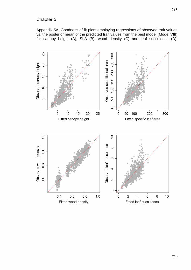
215

215

Chapter 5

Appendix 5A. Goodness of fit plots employing regressions of observed trait values vs. the posterior mean of the predicted trait values from the best model (Model VIII) for canopy height (A), SLA (B), wood density (C) and leaf succulence (D).

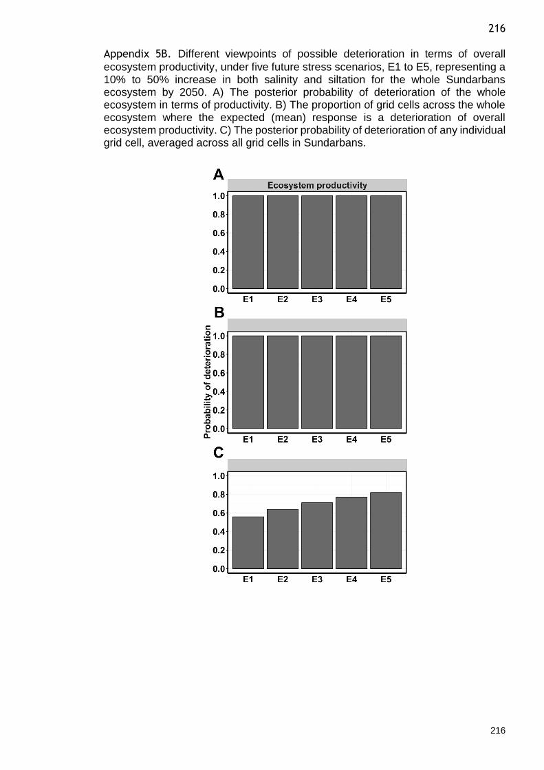
216

216

Appendix 5B. Different viewpoints of possible deterioration in terms of overall

ecosystem productivity, under five future stress scenarios, E1 to E5, representing a 10% to 50% increase in both salinity and siltation for the whole Sundarbans ecosystem by 2050. A) The posterior probability of deterioration of the whole ecosystem in terms of productivity. B) The proportion of grid cells across the whole ecosystem where the expected (mean) response is a deterioration of overall ecosystem productivity. C) The posterior probability of deterioration of any individual grid cell, averaged across all grid cells in Sundarbans.

217

217

Appendix 5C. Different viewpoints of possible deterioration in terms of community

traits, under five future stress scenarios, E1 to E5, representing a 10% to 50% increase in both salinity and siltation for the whole Sundarbans ecosystem by 2050. A) The posterior probability of deterioration of the whole ecosystem in terms of community traits: CH, SLA, WD and LS; B) The proportion of grid cells across the whole ecosystem where the expected (mean) response is a deterioration in terms of the community traits; C) The posterior probability of deterioration of any individual grid cell, averaged across all grid cells in the Sundarbans in terms of the community traits. Decreases in CH and SLA and increases in LS and WD are considered to be deteriorations in the traits.

218

218

Appendix 5D. Different viewpoints of possible deterioration in terms of each of the

traits of the individual species, under five future stress scenarios, E1 to E5, representing a 10% to 50% increase in both salinity and siltation for the whole Sundarbans ecosystem by 2050. A) The posterior probability of deterioration of traits (CH, SLA, WD and LS) for four prominent tree species across the entire ecosystem; B) The proportion of grid cells across the whole ecosystem where the expected (mean) response is a deterioration for each of the traits of the individual species; C) The posterior probability of deterioration of any individual grid cell, averaged across all grid cells in the Sundarbans in terms of each of the traits of the individual species. Decreases in CH and SLA and increases in LS and WD are deteriorations in the traits.

219

219

Appendix 5E. Current and future (2050) density distributions of four mangrove tree

species in the Sundarbans (Chapter 2).

220

220

Appendix 5F. R code for the trait-based models

##### DATA & LIBRARY IMPORT #### library(xlsx) library(runjags) library(sqldf) library(XLConnect) library(XLConnectJars) library(data.table) library(rjags) # Data arrangement db <- dbConnect(SQLite(), dbname="Test.sqlite.JAGS") # database # Importing excel raw data wb <- loadWorkbook("data.xlsx") setMissingValue(wb, value = "NA") Tables <- readWorksheet(wb, sheet = getSheets(wb)) names(Tables) = c("ENVIRONMENT", "SPECIES", "TRAIT") # Names of the data frames str(Tables) # structure of Tables names(Tables) # Names of the elements of Tables # Incerting tables into database with(Tables, { dbWriteTable(conn = db, name = "ENVIRONMENT", value = ENVIRONMENT, row.names = FALSE, overwrite=TRUE) dbWriteTable(conn = db, name = "SPECIES", value = SPECIES, row.names = FALSE,overwrite=TRUE) dbWriteTable(conn = db, name = "TRAIT", value = TRAIT, row.names = FALSE,overwrite=TRUE) }) ## # Creation of overall species, environment and trait data frame sp.en.traits <- dbGetQuery(db,"SELECT ENVIRONMENT_TRAIT,TRAIT.SPECIES_TRAIT, ENVIRONMENT.NH4, ENVIRONMENT.P, ENVIRONMENT.K, ENVIRONMENT. SALINITY, ENVIRONMENT.SILT, ENVIRONMENT.PH,ENVIRONMENT.URP, ENVIRONMENT.HH, TRAIT.HEIGHT, TRAIT.SLA,TRAIT.WD,TRAIT.SC FROM ENVIRONMENT JOIN TRAIT ON ENVIRONMENT.ENVIRONMENT_ENVIRONMENT = TRAIT.ENVIRONMENT_TRAIT WHERE TRAIT.SLA IS NOT NULL AND TRAIT.WD IS NOT NULL AND TRAIT.SC IS NOT NULL AND SPECIES_TRAIT IN ('E_agallocha','H_fomes','C_decandra','X_mekongensis','A. officinalis','A_cucullata', 'B_sexangula','C_ramiflora','S_apetala')") # species that occurred in > 5% of the plots. n<-length(sp.en.traits[,1]) # Sample size vmax<-4 # Number of traits to be considered # Standardizing trait variables CH<-((sp.en.traits$CH-mean(sp.en.traits$CH))/sd(sp.en.traits$CH)) SLA<-((sp.en.traits$SLA-mean(sp.en.traits$SLA))/sd(sp.en.traits$SLA)) WD<-((sp.en.traits$WD-mean(sp.en.traits$WD))/sd(sp.en.traits$WD)) LS<-((sp.en.traits$LS-mean(sp.en.traits$LS))/sd(sp.en.traits$LS)) traits<-as.matrix(cbind(CH,SLA,WD,LS)) # trait matrix # Standardizing trait variables NH4<-((sp.en.traits$NH4-mean(sp.en.traits$NH4))/sd(sp.en.traits$NH4)) P<-((sp.en.traits$P-mean(sp.en.traits$P))/sd(sp.en.traits$P)) K<-((sp.en.traits$K-mean(sp.en.traits$K))/sd(sp.en.traits$K)) SALINITY<-((sp.en.traits$SALINITY-mean(sp.en.traits$SALINITY))/sd(sp.en.traits$SALINITY)) SILT<-((sp.en.traits$SILT-mean(sp.en.traits$SILT))/sd(sp.en.traits$SILT)) PH<-((sp.en.traits$PH-mean(sp.en.traits$PH))/sd(sp.en.traits$PH)) URP<-((sp.en.traits$URP-mean(sp.en.traits$URP))/sd(sp.en.traits$URP)) HH<-((sp.en.traits$HH-mean(sp.en.traits$HH))/sd(sp.en.traits$HH))

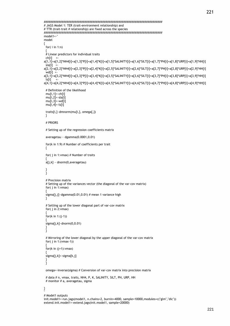
221

221

######################################################################### # JAGS Model 1: TER (trait-environment relationship) and # TTR (trait-trait # relationship) are fixed across the species ######################################################################### model1<-" model { for( i in 1:n) { # Linear predictors for individual traits ch[i] <-a[1,1]+a[1,2]*NH4[i]+a[1,3]*P[i]+a[1,4]*K[i]+a[1,5]*SALINITY[i]+a[1,6]*SILT[i]+a[1,7]*PH[i]+a[1,8]*URP[i]+a[1,9]*HH[i] sla[i] <-a[2,1]+a[2,2]*NH4[i]+a[2,3]*P[i]+a[2,4]*K[i]+a[2,5]*SALINITY[i]+a[2,6]*SILT[i]+a[2,7]*PH[i]+a[2,8]*URP[i]+a[2,9]*HH[i] wd[i] <-a[3,1]+a[3,2]*NH4[i]+a[3,3]*P[i]+a[3,4]*K[i]+a[3,5]*SALINITY[i]+a[3,6]*SILT[i]+a[3,7]*PH[i]+a[3,8]*URP[i]+a[3,9]*HH[i] ls[i] <-a[4,1]+a[4,2]*NH4[i]+a[4,3]*P[i]+a[4,4]*K[i]+a[4,5]*SALINITY[i]+a[4,6]*SILT[i]+a[4,7]*PH[i]+a[4,8]*URP[i]+a[4,9]*HH[i] # Definition of the likelihood mu[i,1]<-ch[i] mu[i,2]<-sla[i] mu[i,3]<-wd[i] mu[i,4]<-ls[i] traits[i,]~dmnorm(mu[i,], omega[,]) } # PRIORS # Setting up of the regression coefficients matrix averagetau ~ dgamma(0.0001,0.01) for(k in 1:9) # Number of coefficients per trait { for( j in 1:vmax) # Number of traits { a[j,k] ~ dnorm(0,averagetau) } } # Precision matrix # Setting up of the variances vector (the diagonal of the var-cov matrix) for( j in 1:vmax) { sigma[j,j]~dgamma(0.01,0.01) # mean 1 variance high } # Setting up of the lower diagonal part of var-cov matrix for( j in 2:vmax) { for(k in 1:(j-1)) { sigma[j,k]~dnorm(0,0.01) } } # Mirroring of the lower diagonal by the upper diagonal of the var-cov matrix for( j in 1:(vmax-1)) { for(k in (j+1):vmax) { sigma[j,k]<-sigma[k,j] } } omega<-inverse(sigma) # Conversion of var-cov matrix into precision matrix # data # n, vmax, traits, NH4, P, K, SALINITY, SILT, PH, URP, HH # monitor # a, averagetau, sigma } " # Model1 outputs init.model1<-run.jags(model1, n.chains=2, burnin=4000, sample=10000,modules=c("glm","dic")) extend.init.model1<-extend.jags(init.model1, sample=20000)

222

222

print(extend.init.model1) dic.extend.init.similar<-extract(extend.init.model1, what='dic') # DIC, pD ######################################################################### # Model 2: TTR varies across the species ######################################################################### species<-as.integer(factor(sp.en.traits$SPECIES)) # species as factors model2<-" model { for( i in 1:n) { # Linear predictors for individual traits ch[i] <-a[1,1]+a[1,2]*NH4[i]+a[1,3]*P[i]+a[1,4]*K[i]+a[1,5]*SALINITY[i]+a[1,6]*SILT[i]+a[1,7]*PH[i]+a[1,8]*URP[i]+a[1,9]*HH[i] sla[i] <-a[2,1]+a[2,2]*NH4[i]+a[2,3]*P[i]+a[2,4]*K[i]+a[2,5]*SALINITY[i]+a[2,6]*SILT[i]+a[2,7]*PH[i]+a[2,8]*URP[i]+a[2,9]*HH[i] wd[i] <-a[3,1]+a[3,2]*NH4[i]+a[3,3]*P[i]+a[3,4]*K[i]+a[3,5]*SALINITY[i]+a[3,6]*SILT[i]+a[3,7]*PH[i]+a[3,8]*URP[i]+a[3,9]*HH[i] ls[i] <-a[4,1]+a[4,2]*NH4[i]+a[4,3]*P[i]+a[4,4]*K[i]+a[4,5]*SALINITY[i]+a[4,6]*SILT[i]+a[4,7]*PH[i]+a[4,8]*URP[i]+a[4,9]*HH[i] # Definition of the likelihood mu[i,1]<-ls[i] mu[i,2]<-sla[i] mu[i,3]<-wd[i] mu[i,4]<-ls[i] traits[i,]~dmnorm(mu[i,], omega[species[i],,]) } # PRIORS # Setting up of the regression coefficients matrix averagetau ~ dgamma(0.0001,0.01) for(k in 1:9) # Number of coefficients per trait { for( j in 1:vmax) # Number of traits { a[j,k] ~ dnorm(0,averagetau) } } # Precision matrix # Setting up of the variances vector (the diagonal of the var-cov matrix) tauvar~dgamma(1.00, 1.00) for( j in 1:vmax) { for (m in 1:9) { sigma[m,j,j]~dgamma(1, 0.01) # mean 1 variance high } } # Setting up of the lower diagonal part of var-cov matrix for( j in 2:vmax) { for(k in 1:(j-1)) { for (m in 1:9) { sigma[m,j,k]~dnorm(0,tauvar) } } } # Mirroring of the lower diagonal by the upper diagonal of the var-cov matrix for( j in 1:(vmax-1)) { for(k in (j+1):vmax) { for (m in 1:9) {

223

223

sigma[m,j,k]<-sigma[m,k,j] } } } for (m in 1:9) { omega[m,1:vmax,1:vmax]<-inverse(sigma[m,1:vmax,1:vmax]) # Conversion of var-cov matrix into precision matrix } # data # n, vmax, traits, NH4, P, K,SALINITY, SILT, PH, URP, HH, species # monitor # a, sigma, tauvar } " # model2 outputs init.model2<-run.jags(model2, n.chains=2, burnin=4000, sample=10000,modules=c("glm","dic")) extend.init.model2<-extend.jags(init.model2, sample=20000) print(extend.init.model2) dic.extend.init.model2<-extract(extend.init.model2, what='dic') # DIC, pD ######################################################################### # Model 3: TER varies across the species ######################################################################### model3<-" model { for( i in 1:n) { # Linear predictors for individual traits ch[i]<-a[1,1,species[i]]+a[1,2,species[i]]*NH4[i]+a[1,3,species[i]]*P[i]+a[1,4,species[i]]*K[i]+a[1,5,species[i]]*SALINITY[i]+a[1,6,species[i]]*SILT[i]+a[1,7,species[i]]*PH[i]+a[1,8,species[i]]*URP[i]+a[1,9,species[i]]*HH[i] sla[i]<-a[2,1,species[i]]+a[2,2,species[i]]*NH4[i]+a[2,3,species[i]]*P[i]+a[2,4,species[i]]*K[i]+a[2,5,species[i]]*SALINITY[i]+a[2,6,species[i]]*SILT[i]+a[2,7,species[i]]*PH[i]+a[2,8,species[i]]*URP[i]+a[2,9,species[i]]*HH[i] wd[i] <-a[3,1,species[i]]+a[3,2,species[i]]*NH4[i]+a[3,3,species[i]]*P[i]+a[3,4,species[i]]*K[i]+a[3,5,species[i]]*SALINITY[i]+a[3,6,species[i]]*SILT[i]+a[3,7,species[i]]*PH[i]+a[3,8,species[i]]*URP[i]+a[3,9,species[i]]*HH[i] ls[i] <-a[4,1,species[i]]+a[4,2,species[i]]*NH4[i]+a[4,3,species[i]]*P[i]+a[4,4,species[i]]*K[i]+a[4,5,species[i]]*SALINITY[i]+a[4,6,species[i]]*SILT[i]+a[4,7,species[i]]*PH[i]+a[4,8,species[i]]*URP[i]+a[4,9,species[i]]*HH[i] # Definition of the likelihood mu[i,1]<-ch[i] mu[i,2]<-sla[i] mu[i,3]<-wd[i] mu[i,4]<-ls[i] traits[i,]~dmnorm(mu[i,], omega[,]) } # PRIORS # Setting up of the regression coefficients matrix tau.b ~ dgamma(0.0001,0.01) for(k in 1:9) # Number of coefficients per trait { for(j in 1:vmax) # Number of traits { for (m in 1:9) { a[j,k,m] ~ dnorm(0,tau.b) } } } # Precision matrix # Setting up of the variances vector (the diagonal of the var-cov matrix) for( j in 1:vmax) { sigma[j,j]~dgamma(0.01,0.01) # mean 1 variance high } # Setting up of the lower diagonal part of var-cov matrix

224

224

for( j in 2:vmax) { for(k in 1:(j-1)) { sigma[j,k]~dnorm(0,0.01) } } # Mirroring of the lower diagonal by the upper diagonal of the var-cov matrix for( j in 1:(vmax-1)) { for(k in (j+1):vmax) { sigma[j,k]<-sigma[k,j] } } omega<-inverse(sigma) # Conversion of var-cov matrix into precision matrix # data # n, vmax, traits, NH4, P, K,SALINITY, SILT, PH, URP, HH, species # monitor # a,tau.b,sigma } " # model3 outputs init.model3<-run.jags(model3, n.chains=2, burnin=4000, sample=10000,modules=c("glm","dic")) extend.init.model3<-extend.jags(init.model3, sample=20000) print(extend.init.model3) dic.extend.init.model3<-extract(extend.init.model3, what='dic') # DIC, pD ######################################################################### # Model 4:TER varies around a common mean ######################################################################### model4<-" model { for( i in 1:n) { # Linear predictors for individual traits ch[i] <-a[1,1,species[i]]+a[1,2,species[i]]*NH4[i]+a[1,3,species[i]]*P[i]+a[1,4,species[i]]*K[i]+a[1,5,species[i]]*SALINITY[i]+a[1,6,species[i]]*SILT[i]+a[1,7,species[i]]*PH[i]+a[1,8,species[i]]*URP[i]+a[1,9,species[i]]*HH[i] sla[i]<-a[2,1,species[i]]+a[2,2,species[i]]*NH4[i]+a[2,3,species[i]]*P[i]+a[2,4,species[i]]*K[i]+a[2,5,species[i]]*SALINITY[i]+a[2,6,species[i]]*SILT[i]+a[2,7,species[i]]*PH[i]+a[2,8,species[i]]*URP[i]+a[2,9,species[i]]*HH[i] wd[i] <-a[3,1,species[i]]+a[3,2,species[i]]*NH4[i]+a[3,3,species[i]]*P[i]+a[3,4,species[i]]*K[i]+a[3,5,species[i]]*SALINITY[i]+a[3,6,species[i]]*SILT[i]+a[3,7,species[i]]*PH[i]+a[3,8,species[i]]*URP[i]+a[3,9,species[i]]*HH[i] ls[i] <-a[4,1,species[i]]+a[4,2,species[i]]*NH4[i]+a[4,3,species[i]]*P[i]+a[4,4,species[i]]*K[i]+a[4,5,species[i]]*SALINITY[i]+a[4,6,species[i]]*SILT[i]+a[4,7,species[i]]*PH[i]+a[4,8,species[i]]*URP[i]+a[4,9,species[i]]*HH[i] # Definition of the likelihood mu[i,1]<-ch[i] mu[i,2]<-sla[i] mu[i,3]<-wd[i] mu[i,4]<-ls[i] traits[i,]~dmnorm(mu[i,], omega[,]) } # PRIORS # Setting up of the regression coefficients matrix averagetau ~ dgamma(0.0001,0.01) tau.a ~ dgamma(0.0001,0.01) for(k in 1:9) # Number of coefficients per trait { for(j in 1:vmax) # Number of traits { averagea[j,k] ~ dnorm(0,averagetau) for (m in 1:9) { a[j,k,m] ~ dnorm(averagea[j,k],tau.a) } } } # Precision matrix

225

225

# Setting up of the variances vector (the diagonal of the var-cov matrix) tauvar~dgamma(1.00, 1.00) for( j in 1:vmax) { sigma[j,j]~dgamma(1, 0.01) # mean 1 variance high } # Setting up of the lower diagonal part of var-cov matrix for( j in 2:vmax) { for(k in 1:(j-1)) { sigma[j,k]~dnorm(0,tauvar) } } # Mirroring of the lower diagonal by the upper diagonal of the var-cov matrix for( j in 1:(vmax-1)) { for(k in (j+1):vmax) { sigma[j,k]<-sigma[k,j] } } omega<-inverse(sigma) # Conversion of var-cov matrix into precision matrix # data # n, vmax, traits, NH4, P, K,SALINITY, SILT, PH, URP, HH, species # monitor # a, averagetau, sigma,tau.a, tauvar } " # model4 outputs init.model4<-run.jags(model4, n.chains=2, burnin=4000, sample=10000,modules=c("glm","dic")) extend.init.model4<-extend.jags(init.model4, sample=20000) print(extend.init.model4) dic.extend.init.model4<-extract(extend.init.model4, what='dic') # DIC, pD ######################################################################### # Model 5: TER varies around the common mean for each trait ######################################################################### model5<-" model { for( i in 1:n) { # Linear predictors for individual traits ch[i] <-a[1,1,species[i]]+a[1,2,species[i]]*NH4[i]+a[1,3,species[i]]*P[i]+a[1,4,species[i]]*K[i]+a[1,5,species[i]]*SALINITY[i]+a[1,6,species[i]]*SILT[i]+a[1,7,species[i]]*PH[i]+a[1,8,species[i]]*URP[i]+a[1,9,species[i]]*HH[i] sla[i]<-a[2,1,species[i]]+a[2,2,species[i]]*NH4[i]+a[2,3,species[i]]*P[i]+a[2,4,species[i]]*K[i]+a[2,5,species[i]]*SALINITY[i]+a[2,6,species[i]]*SILT[i]+a[2,7,species[i]]*PH[i]+a[2,8,species[i]]*URP[i]+a[2,9,species[i]]*HH[i] wd[i] <-a[3,1,species[i]]+a[3,2,species[i]]*NH4[i]+a[3,3,species[i]]*P[i]+a[3,4,species[i]]*K[i]+a[3,5,species[i]]*SALINITY[i]+a[3,6,species[i]]*SILT[i]+a[3,7,species[i]]*PH[i]+a[3,8,species[i]]*URP[i]+a[3,9,species[i]]*HH[i] ls[i] <-a[4,1,species[i]]+a[4,2,species[i]]*NH4[i]+a[4,3,species[i]]*P[i]+a[4,4,species[i]]*K[i]+a[4,5,species[i]]*SALINITY[i]+a[4,6,species[i]]*SILT[i]+a[4,7,species[i]]*PH[i]+a[4,8,species[i]]*URP[i]+a[4,9,species[i]]*HH[i] # Definition of the likelihood mu[i,1]<-ch[i] mu[i,2]<-sla[i] mu[i,3]<-wd[i] mu[i,4]<-ls[i] traits[i,]~dmnorm(mu[i,], omega[,]) } # PRIORS # Setting up of the regression coefficients matrix averagetau ~ dgamma(0.0001,0.01) for(j in 1:vmax) # Number of traits { tau[j] ~ dgamma(0.0001,0.01)

226

226

for(k in 1:9) # Number of coefficients per trait { averagea[j,k] ~ dnorm(0,averagetau) for (m in 1:9) { a[j,k,m] ~ dnorm(averagea[j,k],tau[j]) } } } # Precision matrix # Setting up of the variances vector (the diagonal of the var-cov matrix) tauvar~dgamma(1.00, 1.00) for( j in 1:vmax) { sigma[j,j]~dgamma(1, 0.01) # mean 1 variance high } # Setting up of the lower diagonal part of var-cov matrix for( j in 2:vmax) { for(k in 1:(j-1)) { sigma[j,k]~dnorm(0,tauvar) } } # Mirroring of the lower diagonal by the upper diagonal of the var-cov matrix for( j in 1:(vmax-1)) { for(k in (j+1):vmax) { sigma[j,k]<-sigma[k,j] } } omega<-inverse(sigma) # Conversion of var-cov matrix into precision matrix # data # n, vmax, traits, NH4, P, K,SALINITY, SILT, PH, URP, HH, species # monitor # a, averagea, sigma,tau, tauvar } " # model5 results init.model5<-run.jags(model5, n.chains=2, burnin=4000, sample=10000,modules=c("glm","dic")) extend.init.model5<-extend.jags(init.model5, sample=20000) print(extend.init.model5) dic.extend.init.model5<-extract(extend.init.model5, what='dic') # DIC, pD ######################################################################### # Model 6: TER varies around the common mean for each environmental driver ######################################################################### model6<-" model { for( i in 1:n) { # Linear predictors for individual traits ch[i] <-a[1,1,species[i]]+a[1,2,species[i]]*NH4[i]+a[1,3,species[i]]*P[i]+a[1,4,species[i]]*K[i]+a[1,5,species[i]]*SALINITY[i]+a[1,6,species[i]]*SILT[i]+a[1,7,species[i]]*PH[i]+a[1,8,species[i]]*URP[i]+a[1,9,species[i]]*HH[i] sla[i]<-a[2,1,species[i]]+a[2,2,species[i]]*NH4[i]+a[2,3,species[i]]*P[i]+a[2,4,species[i]]*K[i]+a[2,5,species[i]]*SALINITY[i]+a[2,6,species[i]]*SILT[i]+a[2,7,species[i]]*PH[i]+a[2,8,species[i]]*URP[i]+a[2,9,species[i]]*HH[i] wd[i] <-a[3,1,species[i]]+a[3,2,species[i]]*NH4[i]+a[3,3,species[i]]*P[i]+a[3,4,species[i]]*K[i]+a[3,5,species[i]]*SALINITY[i]+a[3,6,species[i]]*SILT[i]+a[3,7,species[i]]*PH[i]+a[3,8,species[i]]*URP[i]+a[3,9,species[i]]*HH[i] ls[i] <-a[4,1,species[i]]+a[4,2,species[i]]*NH4[i]+a[4,3,species[i]]*P[i]+a[4,4,species[i]]*K[i]+a[4,5,species[i]]*SALINITY[i]+a[4,6,species[i]]*SILT[i]+a[4,7,species[i]]*PH[i]+a[4,8,species[i]]*URP[i]+a[4,9,species[i]]*HH[i] # Definition of the likelihood mu[i,1]<-ch[i] mu[i,2]<-sla[i] mu[i,3]<-wd[i] mu[i,4]<-ls[i]

227

227

traits[i,]~dmnorm(mu[i,], omega[,]) } # PRIORS # Setting up of the regression coefficients matrix averagetau ~ dgamma(0.0001,0.01) for(k in 1:9) # Number of coefficients per trait { tau[k] ~ dgamma(0.0001,0.01) for(j in 1:vmax) # Number of traits { averagea[j,k] ~ dnorm(0,averagetau) for (m in 1:9) { a[j,k,m] ~ dnorm(averagea[j,k],tau[k]) } } } # Precision matrix # Setting up of the variances vector (the diagonal of the var-cov matrix) tauvar~dgamma(1.00, 1.00) for( j in 1:vmax) { sigma[j,j]~dgamma(1, 0.01) # mean 1 variance high } # Setting up of the lower diagonal part of var-cov matrix for( j in 2:vmax) { for(k in 1:(j-1)) { sigma[j,k]~dnorm(0,tauvar) } } # Mirroring of the lower diagonal by the upper diagonal of the var-cov matrix for( j in 1:(vmax-1)) { for(k in (j+1):vmax) { sigma[j,k]<-sigma[k,j] } } omega<-inverse(sigma) # Conversion of var-cov matrix into precision matrix # data # n, vmax, traits, NH4, P, K,SALINITY, SILT, PH, URP, HH, species # monitor # a, averagea, sigma,tau, tauvar } " # model6 outputs init.model6<-run.jags(model6, n.chains=2, burnin=4000, sample=10000,modules=c("glm","dic")) extend.init.model6<-extend.jags(init.model6, sample=20000) print(extend.init.model6) dic.extend.init.model6<-extract(extend.init.model6, what='dic') # DIC, pD ######################################################################### # Model 7: TER varies around the common mean for each trait and environmental driver ######################################################################### model7<-" model { for( i in 1:n) { # Linear predictors for individual traits ch[i] <-a[1,1,species[i]]+a[1,2,species[i]]*NH4[i]+a[1,3,species[i]]*P[i]+a[1,4,species[i]]*K[i]+a[1,5,species[i]]*SALINITY[i]+a[1,6,species[i]]*SILT[i]+a[1,7,species[i]]*PH[i]+a[1,8,species[i]]*URP[i]+a[1,9,species[i]]*HH[i]

228

228

sla[i]<-a[2,1,species[i]]+a[2,2,species[i]]*NH4[i]+a[2,3,species[i]]*P[i]+a[2,4,species[i]]*K[i]+a[2,5,species[i]]*SALINITY[i]+a[2,6,species[i]]*SILT[i]+a[2,7,species[i]]*PH[i]+a[2,8,species[i]]*URP[i]+a[2,9,species[i]]*HH[i] wd[i] <-a[3,1,species[i]]+a[3,2,species[i]]*NH4[i]+a[3,3,species[i]]*P[i]+a[3,4,species[i]]*K[i]+a[3,5,species[i]]*SALINITY[i]+a[3,6,species[i]]*SILT[i]+a[3,7,species[i]]*PH[i]+a[3,8,species[i]]*URP[i]+a[3,9,species[i]]*HH[i] ls[i] <-a[4,1,species[i]]+a[4,2,species[i]]*NH4[i]+a[4,3,species[i]]*P[i]+a[4,4,species[i]]*K[i]+a[4,5,species[i]]*SALINITY[i]+a[4,6,species[i]]*SILT[i]+a[4,7,species[i]]*PH[i]+a[4,8,species[i]]*URP[i]+a[4,9,species[i]]*HH[i] # Definition of the likelihood mu[i,1]<-ch[i] mu[i,2]<-sla[i] mu[i,3]<-wd[i] mu[i,4]<-ls[i] traits[i,]~dmnorm(mu[i,], omega[,]) } # PRIORS # Setting up of the regression coefficients matrix averagetau ~ dgamma(0.0001,0.01) for(k in 1:9) # Number of coefficients per trait { for(j in 1:vmax) # Number of traits { tau[j,k] ~ dgamma(0.0001,0.01) averagea[j,k] ~ dnorm(0,averagetau) for (m in 1:9) { a[j,k,m] ~ dnorm(averagea[j,k],tau[j,k]) } } } # Precision matrix # Setting up of the variances vector (the diagonal of the var-cov matrix) tauvar~dgamma(1.00, 1.00) for( j in 1:vmax) { sigma[j,j]~dgamma(1, 0.01) # mean 1 variance high } # Setting up of the lower diagonal part of var-cov matrix for( j in 2:vmax) { for(k in 1:(j-1)) { sigma[j,k]~dnorm(0,tauvar) } } # Mirroring of the lower diagonal by the upper diagonal of the var-cov matrix for( j in 1:(vmax-1)) { for(k in (j+1):vmax) { sigma[j,k]<-sigma[k,j] } } omega<-inverse(sigma) # Conversion of var-cov matrix into precision matrix # data # n, vmax, traits, NH4, P, K,SALINITY, SILT, PH, URP, HH, species # monitor # a, averagea, sigma,tau, tauvar } " # model7 outputs init.model7<-run.jags(model7, n.chains=2, burnin=4000, sample=10000,modules=c("glm","dic")) extend.init.model7<-extend.jags(init.model7, sample=20000) print(extend.init.model7) dic.extend.init.model7<-extract(extend.init.model7, what='dic') # DIC

229

229

######################################################################### # Model 8: TTR varies across the species ######################################################################### model8<-" model { for( i in 1:n) { # Linear predictors for individual traits ch[i] <-a[1,1,species[i]]+a[1,2,species[i]]*NH4[i]+a[1,3,species[i]]*P[i]+a[1,4,species[i]]*K[i]+a[1,5,species[i]]*SALINITY[i]+a[1,6,species[i]]*SILT[i]+a[1,7,species[i]]*PH[i]+a[1,8,species[i]]*URP[i]+a[1,9,species[i]]*HH[i] sla[i]<-a[2,1,species[i]]+a[2,2,species[i]]*NH4[i]+a[2,3,species[i]]*P[i]+a[2,4,species[i]]*K[i]+a[2,5,species[i]]*SALINITY[i]+a[2,6,species[i]]*SILT[i]+a[2,7,species[i]]*PH[i]+a[2,8,species[i]]*URP[i]+a[2,9,species[i]]*HH[i] wd[i] <-a[3,1,species[i]]+a[3,2,species[i]]*NH4[i]+a[3,3,species[i]]*P[i]+a[3,4,species[i]]*K[i]+a[3,5,species[i]]*SALINITY[i]+a[3,6,species[i]]*SILT[i]+a[3,7,species[i]]*PH[i]+a[3,8,species[i]]*URP[i]+a[3,9,species[i]]*HH[i] ls[i] <-a[4,1,species[i]]+a[4,2,species[i]]*NH4[i]+a[4,3,species[i]]*P[i]+a[4,4,species[i]]*K[i]+a[4,5,species[i]]*SALINITY[i]+a[4,6,species[i]]*SILT[i]+a[4,7,species[i]]*PH[i]+a[4,8,species[i]]*URP[i]+a[4,9,species[i]]*HH[i] # Definition of the likelihood mu[i,1]<-ch[i] mu[i,2]<-sla[i] mu[i,3]<-wd[i] mu[i,4]<-ls[i] traits[i,]~dmnorm(mu[i,], omega[species[i],,]) } # PRIORS # Setting up of the regression coefficients matrix averagetau ~ dgamma(0.0001,0.01) for(k in 1:9) # Number of coefficients per trait { tau[k] ~ dgamma(0.0001,0.01) for(j in 1:vmax) # Number of traits { averagea[j,k] ~ dnorm(0,averagetau) for (m in 1:9) { a[j,k,m] ~ dnorm(averagea[j,k],tau[k]) } } } # Precision matrix # Setting up of the variances vector (the diagonal of the var-cov matrix) tauvar~dgamma(1.00, 1.00) for( j in 1:vmax) { for (m in 1:9) { sigma[m,j,j]~dgamma(1, 0.01) # mean 1 variance high } } # Setting up of the lower diagonal part of var-cov matrix for( j in 2:vmax) { for(k in 1:(j-1)) { for (m in 1:9) { sigma[m,j,k]~dnorm(0,tauvar) } } } # Mirroring of the lower diagonal by the upper diagonal of the var-cov matrix

230

230

for( j in 1:(vmax-1)) { for(k in (j+1):vmax) { for (m in 1:9) { sigma[m,j,k]<-sigma[m,k,j] } } } for (m in 1:9) { omega[m,1:vmax,1:vmax]<-inverse(sigma[m,1:vmax,1:vmax]) # Conversion of var-cov matrix into precision matrix } # data # n, vmax, traits, NH4, P, K,SALINITY, SILT, PH, URP, HH, species # monitor # a, averagetau, sigma, tauvar } " # model8 outputs init.model8<-run.jags(model8, n.chains=2, burnin=4000, sample=10000,modules=c("glm","dic")) extend.init.model8<-extend.jags(init.model8, sample=20000) print(extend.init.model8) dic.extend.init.model8<-extract(extend.init.model8, what='dic') # DIC, pD ######################################################################### # Model 9: TTR varies around a common mean ######################################################################### model9<-" model { for( i in 1:n) { # Linear predictors for individual traits ch[i] <-a[1,1,species[i]]+a[1,2,species[i]]*NH4[i]+a[1,3,species[i]]*P[i]+a[1,4,species[i]]*K[i]+a[1,5,species[i]]*SALINITY[i]+a[1,6,species[i]]*SILT[i]+a[1,7,species[i]]*PH[i]+a[1,8,species[i]]*URP[i]+a[1,9,species[i]]*HH[i] sla[i]<-a[2,1,species[i]]+a[2,2,species[i]]*NH4[i]+a[2,3,species[i]]*P[i]+a[2,4,species[i]]*K[i]+a[2,5,species[i]]*SALINITY[i]+a[2,6,species[i]]*SILT[i]+a[2,7,species[i]]*PH[i]+a[2,8,species[i]]*URP[i]+a[2,9,species[i]]*HH[i] wd[i] <-a[3,1,species[i]]+a[3,2,species[i]]*NH4[i]+a[3,3,species[i]]*P[i]+a[3,4,species[i]]*K[i]+a[3,5,species[i]]*SALINITY[i]+a[3,6,species[i]]*SILT[i]+a[3,7,species[i]]*PH[i]+a[3,8,species[i]]*URP[i]+a[3,9,species[i]]*HH[i] ls[i] <-a[4,1,species[i]]+a[4,2,species[i]]*NH4[i]+a[4,3,species[i]]*P[i]+a[4,4,species[i]]*K[i]+a[4,5,species[i]]*SALINITY[i]+a[4,6,species[i]]*SILT[i]+a[4,7,species[i]]*PH[i]+a[4,8,species[i]]*URP[i]+a[4,9,species[i]]*HH[i] # Definition of the likelihood mu[i,1]<-CH[i] mu[i,2]<-sla[i] mu[i,3]<-wd[i] mu[i,4]<-sc[i] traits[i,]~dmnorm(mu[i,], omega[species[i],,]) } # PRIORS # Setting up of the regression coefficients matrix averagetau ~ dgamma(0.0001,0.01) for(k in 1:9) # Number of coefficients per trait { tau[k] ~ dgamma(0.0001,0.01) for(j in 1:vmax) # Number of traits { averagea[j,k] ~ dnorm(0,averagetau) for (m in 1:9) { a[j,k,m] ~ dnorm(averagea[j,k],tau[k]) } } }

231

231

# Precision matrix # Setting up of the variances vector (the diagonal of the var-cov matrix) tauvar~dgamma(1.00, 1.00) tau.c~dgamma(0.0001,0.01) for( j in 1:vmax) { for (m in 1:9) { sigma[m,j,j]~dgamma(1, 0.01) # mean 1 variance high } } # Setting up of the lower diagonal part of var-cov matrix for( j in 2:vmax) { for(k in 1:(j-1)) { avsigma[j,k]~dnorm(0,tauvar) for (m in 1:9) { sigma[m,j,k]~dnorm(avsigma[j,k],tau.c) } } } # Mirroring of the lower diagonal by the upper diagonal of the var-cov matrix for( j in 1:(vmax-1)) { for(k in (j+1):vmax) { for (m in 1:9) { sigma[m,j,k]<-sigma[m,k,j] } } } for (m in 1:9) { omega[m,1:vmax,1:vmax]<-inverse(sigma[m,1:vmax,1:vmax]) # Conversion of var-cov matrix into precision matrix } # data # n, vmax, traits, NH4, P, K,SALINITY, SILT, PH, URP, HH, species # monitor # a, averagea,sigma,tauvar,tau.c } " # model9 outputs init.model9<-run.jags(model9, n.chains=2, burnin=4000, sample=10000,modules=c("glm","dic")) extend.init.model9<-extend.jags(init.model9, sample=20000) print(extend.init.model9) dic.extend.init.model9<-extract(extend.init.model9, what='dic') # DIC, pD